Bayesian Hierarchical Linear Modeling of Profile Data with ...imse.utep.edu/mdasi/paper/paper8.pdf · Profile Data with Applications to Quality Control of Nanomanufacturing ... microstructural

> REPLACE THIS LINE WITH YOUR PAPER IDENTIFICATION NUMBER (DOUBLE-CLICK HERE TO EDIT) <

1

Abstract— In this article, we propose to use the multiple

ultrasonic attenuation profiles measured at different locations of a

specimen to infer the microstructure of metal-matrix

nanocomposites. We present a general framework to connect the

profile data with both explanatory variables and product quality

parameters for quality inference. More specifically, a hierarchical

linear model with level-2 variance heterogeneity is proposed to

model the relationship between ultrasonic attenuation profiles,

ultrasonic frequency, and the microstructural parameters of the

nanocomposites. An integrated Bayesian framework for model

estimation, model selection, and inference of the microstructural

parameters is proposed through blocked Gibbs sampling,

intrinsic Bayes factor, and importance sampling. The effectiveness

of the proposed approach is illustrated through case studies.

Note to Practitioners— This paper was motivated by the

problem of inspecting and controlling the microstructural quality

of aluminum alloy based nanocomposites using ultrasonic

attenuation profiles. One critical quality issue in the

nanocomposite manufacturing is the uniformity and completeness

of the nanoparticle dispersion which directly influence the

homogeneity and grain refinement of nanocomposites. The

standard quality inspection technique is to use microscopic images

of microstructures, which are costly and time-consuming to

obtain. Multiple attenuation profiles measured at sampled

locations of the specimen surface contain rich information about

the microstructural quality (e.g., grain size, homogeneity) and

thus can be used for quality inference and control. This paper

proposes a general multi-level regression model to characterize

the relationship between the functional response variable (e.g.,

attenuation), explanatory variables (e.g., frequency), and the

microstructural parameters of products (e.g., grain size) for

quality inference. An efficient general Monte Carlo simulation

approach under the Bayesian framework is developed to estimate

the model parameters, to select the optimal models, and to infer

the microstructural quality parameters for inspection. The

proposed methodology is shown to be very effective in quality

inspection through numerical and case study. It may have broad

applications where the quality can be sufficiently characterized by

multiple profiles.

This work was supported by National Science Foundation under grant

1335129 J. Wu is with the Department of Industrial, Manufacturing and Systems

Engineering, University of Texas at El Paso, TX79968 USA (email:

[email protected]). Y. Liu and S. Zhou are with the Department Industrial and Systems

Engineering, University of Wisconsin-Madison, WI 53706 USA (email:

[email protected]; [email protected]).

Index Terms—Hierarchical linear model, Variance

heterogeneity, Monte Carlo Markov chain, Gibbs sampling,

Model selection, Metal-matrix nanocomposites, Quality control,

Profile monitoring

I. INTRODUCTION

HERE is a rapidly growing demand for structural

components of high performance lightweight materials in

the automotive, aerospace, and many other industries.

A206-Al2O3 metal matrix nanocomposites (MMNCs) are

promising lightweight metallic materials, which can be

fabricated by dispersing Al2O3 nanoparticles into molten A206

alloys (93.5%-95% Al, 4.2%-5.0% Cu) in the ultrasonic

cavitation based casting technologies [1, 2]. Well-dispersed

Al2O3 nanoparticles in the molten A206 alloy can enhance the

nucleation of both α-Al primary phase and β-Al2Cu

intermetallic phase, which leads to significantly improved

mechanical properties and castablity, e.g., high strength,

ductility, long fatigue life, and hot tearing resistance [3]. One

critical quality issue in the nanocomposites manufacturing is

the uniformity and completeness of the nanoparticle dispersion.

Due to their high surface energy, large surface-to-volume ratio

and poor wettability in molten metal, nanoparticles tend to

agglomerate and cluster together, which greatly limits their

effectiveness in microstructural morphology modification and

property improvement [4, 5].

The conventional quality inspection method for

nanocomposites is based on microscopic images, which are

costly and time-consuming to obtain. To facilitate a scale-up

production, it is highly desirable to develop a fast-yet-effective

quality inspection and control technique. Recently Wu et al [6]

investigated the feasibility of relating the ultrasonic attenuation

profiles measured using spectral ratio technique [7] with the

microstructures of A206-Al2O3 MMNCs for quality inspection.

It was found that specimen with more homogeneous

microstructure (i.e., smaller grain size, thinner and less

continuous Al2Cu intermetallic phase, and well-dispersed

Al2O3 nanoparticles) has lower between-curve variation of

attenuation profiles measured at multiple sampled locations.

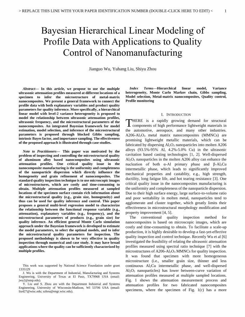
Fig. 1 shows the attenuation measurement process and

attenuation profiles for two fabricated nanocomposites

specimens, where the specimen of Fig. 1(c) has a more

Bayesian Hierarchical Linear Modeling of

Profile Data with Applications to Quality

Control of Nanomanufacturing

Jianguo Wu, Yuhang Liu, Shiyu Zhou

T

mailto:[email protected]

mailto:[email protected]


2

homogeneous microstructure than that of Fig. 1(b). The

phenomenon of more homogeneous microstructures resulting

in less variation has also been observed by Liu et al [8] through

microstructural modeling and wave propagation simulation

approach. Therefore, the microstructural quality of MMNCs

can be characterized by multiple attenuation profiles measured

at different locations. Quality characterization based on

multiple profiles measured at randomly sampled locations has

also been studied in low-E glass manufacturing, where the

uniformity of coating on the glass surface could be captured by

multiple spectral reflectance profiles [9].

Fig. 1. Attenuation measurement and attenuation profiles measured at sampled locations: (a) spectral ratio technique for attenuation profile measurement; (b) A206

nanocomposites with 1wt% of Al2O3 nanoparticles, (c) A206 nanocomposites with 5wt% of Al2O3 nanoparticles.

Profile data has been widely used for quality monitoring and

control of manufacturing processes where products quality can

be sufficiently characterized by profiles [10-12]. Various

mathematical models have been proposed to describe profile

data, including (1) simple or multiple linear profiles (e.g.,

polynomials) where a single or multiple explanatory variables

are used to describe the behavior of the response variable, (2)

parametric nonlinear profiles, (3) nonparametric nonlinear

profiles (e.g., splines, wavelets), (4) multivariate linear profiles

where a set of response variables are linear functions of

explanatory variables, and (5) binary response profiles. In most

of the existing profile data modeling approaches, the

covariance matrix of coefficients is assumed to be unchanged,

and only a single profile is modeled. Very limited research has

been conducted to model the covariance matrix or the

between-profile variations. To characterize the uniformity of a

product such as the nanocomposites, however, a single profile

is often not enough, and multiple profiles of the same response

variable measured at multiple sampled locations of a product

have to be used and modeled.

To fill the gap, we propose a hierarchical linear model

(HLM), or more specifically a two-level model, with

heterogeneous level-2 variances to infer the microstructural

quality in the nanocomposites manufacturing. There are three

parts in the proposed model: (1) the profile is modeled as a

linear function of explanatory variables in level-1; (2) the

coefficients in level-1 are modeled as linear functions of

microstructural parameters in level-2 with diagonal residual

covariance matrix; (3) the residual variances in level-2 are

modeled as log-linear function of microstructural parameters.

The model with only the first two parts is a hierarchical linear

model, which is a variant term for multilevel model or for what

are broadly called linear mixed-effects (LME) model. In this

paper, we use the term HLM instead of LME to differentiate the

new model from the common LME model used in [9]. The third

part is an embedded variance regression model to characterize

the heterogeneity of the variance of coefficients across different

microstructural parameters. Compared with the traditional

LME model used in profile monitoring [9, 13], our model has

the advantage of directly relating the microstructural

parameters with profiles for quality inference.

HLM has been widely used to model hierarchically

structured data in the biomedical and social research [14, 15].

Extensions of the HLM with heterogeneous within-profile

noise variances (e.g., residual variance in level-1 model) have

also been intensively studied [16-18]. However, there is very

limited work on modeling heterogeneous variances for random

effects. For the standard HLM, The model parameters can be

estimated using two general methods, maximum likelihood

(ML) and restricted maximum likelihood (REML) [19].

However, these methods cannot be directly applied to the

proposed model, as the addition of the third part of the model

makes the optimization much more complicated. The

remaining challenges of the proposed model are model

selection (e.g., determining the degree of polynomial, which

coefficient is random), and inference of the microstructural

parameters of new profiles in real-time monitoring. In this

paper, we propose to use Markov chain Monte Carlo (MCMC)

approach under the Bayesian framework, which can not only

estimate the model parameters, but also perform model

1.7 1.9 2.1 2.3 2.50

0.1

0.2

0.3

0.4

Frequency (MHz)

Att

en

ua

tio

n (

dB

/mm

)

Transducer

0 2 4 6 8-100

-50

0

50

100

Time (s)

Am

pli

tud

e (

mV

)

S1(t)

S2(t)

(b) (c)

(a)


3

selection and inference of the microstructural parameters

efficiently and accurately.

The remainder of the paper is organized as follows. In

Section II the new HLM with heterogeneous level-2 variances

is formulated. The MCMC estimation of model parameters and

model selection are given in Section III and Section IV

respectively. Section V evaluates the performance of model

selection and estimation through numerical simulations.

Section VI presents the case study where the proposed model is

applied to the ultrasonic attenuation profiles of MMNCs. The

conclusions and discussions are given in Section VII.

II. TWO-LEVEL HIERARCHICAL LINEAR MODEL WITH

HETEROGENEOUS LEVEL-2 VARIANCES

Fig. 2. Illustration of the hierarchical data structure.

Fig. 2 shows the hierarchical data structure. Suppose the

profiles are obtained from 𝑚 different specimens or products,

where each specimen was measured multiple times at multiple

sampled locations. For each measuring location we obtain one

profile. Without loss of generosity, we assume that each

specimen has 𝑙 profiles and each profile has 𝑛 observations at 𝑛

fixed locations for all profiles. Let 𝜽𝑖 be the vector of

microstructural parameters of the i-th specimen, 𝒚𝑖𝑗 be the j-th

profile of specimen i, and 𝑥𝑘 be the 𝑘-th design point. The

hierarchical linear model with heterogeneous level-2 variances

is defined as follows:

Level-1:

𝑦𝑖𝑗𝑘 = 𝒉1′ (𝒙𝑘)𝜶𝑖𝑗 + 𝜖𝑖𝑗𝑘 (1)

where 𝑖 = 1,… ,𝑚 is the index of specimens, 𝑗 = 1,… , 𝑙 is the

index of profiles, and 𝑘 = 1,… , 𝑛 is the index of frequencies,

𝒉1(𝑥) is a vector of 𝑝 predictor variables at 𝑥, e.g., 𝒉1(𝑥) =(𝑥2, 𝑥, 1)′ for quadratic polynomial, 𝜶𝑖𝑗 is a 𝑝 × 1 vector of

regression coefficients, and 𝜖𝑖𝑗𝑘 is the within-profile error

which follows i.i.d. Gaussian distribution, 𝜖𝑖𝑗𝑘~𝑁(0, 𝜎𝜖2).

Level-2:

𝜶𝑖𝑗 = 𝑯2(𝜽𝑖)𝜷 + 𝝃𝑖𝑗 (2)

where 𝑯2(𝜽𝑖) = 𝑰𝑝⊗𝒉2𝑇(𝜽𝑖) is a 𝑝 × 𝑝𝑞 matrix ( ⊗ :

Kronecker product operator), 𝒉2(𝜽𝑖) is a 𝑞 × 1 vector of 𝑞

predictor variables, 𝜷 = (𝜷1′ , … , 𝜷𝑝

′ )′ with 𝜷𝑑 being a 𝑞 × 1

vector of regression coefficients for d-th component of 𝜶, and

𝝃𝒊𝒋 is the error term, which is a random vector following i.i.d.

p-dimensional Gaussian distribution for each 𝑖:

𝝃𝑖𝑗~𝑁(𝟎, 𝜮𝑖) (3)

Submodel (2) is used to model the dependence of coefficients

in submodel (1) on the microstructural parameter 𝜽 by the

mean term 𝑯2(𝜽𝑖)𝜷 , and to account for variation among

profiles of the same specimen by the error term 𝝃𝑖𝑗. Combining

(1) and (2) we obtained the general LME model as

𝒚𝑖𝑗 = 𝑯1(𝒙)𝑯2(𝜽𝒊)𝜷 + 𝑯1(𝒙)𝝃𝑖𝑗 + 𝝐𝑖𝑗 (4)

where 𝒚𝑖𝑗 = (𝑦𝑖𝑗1 , … , 𝑦𝑖𝑗𝑛)′

, 𝒙 = (𝑥1, … , 𝑥𝑛)′ , 𝑯1(𝒙) =

(𝒉1(𝑥1),… , 𝒉1(𝑥𝑛))′, and 𝝐𝑖𝑗~𝑵(𝟎, 𝜎𝜖

2𝑰𝒏).

Heterogeneous Level-2 Variances:

To model the variance heterogeneity, we assume the covariance

matrix 𝜮𝑖 in (3) is dependent on the microstructural parameter

𝜽, which is modeled as

𝜮𝑖 = diag(𝜎12(𝜽𝑖), … , 𝜎𝑝

2(𝜽𝑖))

log 𝜎𝑑2 = 𝒉3(𝜽)

′𝜸𝑑 + 𝛿𝑑, 𝑑 = 1,2, … , 𝑝 (5)

where 𝒉3(𝜽) is the 𝑟 × 1 vector of explanatory variables, 𝜸𝑑 is

a 𝑟 × 1 vector of coefficients, and 𝛿𝑑~𝑁(0, 𝜎𝛿𝑑2 ). This part is

used to model the heterogeneity of residual variance in (2). We

select the log-linear model here as it is commonly used in

variance function regression or heteroscedastic regression [20,

21]. Note that we ignore the correlation components in the

covariance matrix 𝛴𝑖, which is a common way to reduce the

model complexity in Bayesian hierarchical models [9, 22]. If

we consider all the correlation components, there will be 𝑝(𝑝 +1)/2 submodels in the variance heterogeneity. Although

ignoring correlations may give a biased estimate of covariance

matrix, it can significantly simplifies the model and avoid the

errors caused by estimating a large number of parameters.

In the proposed model, level-1 is to model each individual

profile or within-profile variations, level-2 is to model both the

model heterogeneity across different specimens and the

between-profile variations within each specimen, and the

log-linear model is to capture the residual variance

heterogeneity of level-2 model. Note that our work share some

similarity with the work proposed by Castillo et al [23] to

optimize the shape of profiles with both controllable factors and

noise factors. The main differences between these two are that

in the model proposed here all design parameters are

controllable and the extra variance heterogeneity model in the

second level is considered. Therefore in our model multiple

profiles at each design point 𝜃𝑖 are needed for model estimation

and the model estimation is much more complicated.

After the new model is proposed, the remaining issues are

how to efficiently estimate the model parameters and how to

accurately select the right models among a set of candidate

ones. In the model estimation, the parameters of interest include

the fixed effects 𝜷 , within-profile error term variance 𝜎𝜖2 ,

variance component regression coefficients {𝜸𝑑 , 𝑑 = 1,… , 𝑝}

Specimen 1 (𝜽1)

Profile 1 (𝒚11) ….

Obs. 1 (𝑦111) ….

Profile l (𝒚1 )

Obs. n (𝑦11𝑛)

….

….

….

Specimen m (𝜽 )

Profile 1 (𝒚 1) ….

Obs. 1 (𝑦 1) ….

Profile l (𝒚 )

Obs. n (𝑦 𝑛)


4

and error term variances {𝜎𝛿𝑑2 , 𝑑 = 1,… , 𝑝} . Denote 𝝍 =

{𝜷, 𝜎𝜖2, {𝜸𝑑}, {𝜎𝛿𝑑

2 }}. The likelihood function for the model can

be expressed by integrating out the nuisance parameters, i.e., all

unobservable random effects 𝝃 = {𝝃𝑖𝑗 , 𝑖 = 1, … ,𝑚, 𝑗 = 1,… , 𝑙}

and variance components 𝝈𝝃𝟐 = {𝜎𝑑

2(𝜽𝑖), 𝑖 = 1,… ,𝑚, 𝑑 =

1,… , 𝑝}, as

𝐿(𝝍|𝒀) = ∫𝑓(𝒀|𝝍, 𝝃, 𝝈𝝃𝟐) 𝑓(𝝃|𝝈𝝃

𝟐, 𝝍)𝑓(𝝈𝝃𝟐|𝝍)𝑑𝝈𝝃

𝟐𝑑𝝃 (6)

where 𝒀 is the vector of all observations, 𝒀 =(𝒚11𝑇 , 𝒚12

𝑇 , … , 𝒚1 𝑇 , … , 𝒚

𝑇 )𝑇 . Equation (6) involves high

dimensional integration and is not analytically tractable, which

makes the maximum likelihood estimation very challenging. In

the research, we propose to estimate the model parameters

under the Bayesian framework. The posterior distribution of the

models parameters are approximated using blocked Gibbs

sampling method, which will be given in detail in the following

section. The second issue is model selection, where the

predictor variables, or the degrees of polynomials if polynomial

regression is used, for all three submodels have to be

determined. Section 4 will present it in detail.

III. BAYESIAN MODEL ESTIMATION USING BLOCKED GIBBS

SAMPLER

A. Specification of Priors

In the Bayesian analysis of the proposed model, the priors for

the mean parameters 𝜷, and {𝜸𝑑 , 𝑑 = 1,… , 𝑝}, and variance

parameters 𝜎𝜖2 and {𝜎𝛿𝑑

2 , 𝑑 = 1,… , 𝑝} need to be specified. For

the mean parameters, the normal priors and noninformative

priors are most commonly used in the Bayesian linear

regression [24]. The normal priors often provide the benefit of

conjugacy in the simple linear regression or conditional

conjugacy, i.e., conjugate prior conditioning on other model

parameters, in the hierarchical linear regression. However, in

most cases the prior information beyond the data is not

available, and thus the noninformative prior is more preferred,

which provides both objectiveness and convenience in

Bayesian analysis. In this research, we specify noninformative

priors for 𝜷 and {𝜸𝑑 , 𝑑 = 1,… , 𝑝} as

𝜋(𝜷) ∝ 1

𝜋(𝜸𝑑) ∝ 1, 𝑑 = 1,… , 𝑝 (7)

For the variance components, there is a lot of literature

discussing how to select appropriate priors [9, 25, 26]. Two

types of priors have been widely used, the noninformative prior

of the form

𝜋(𝜎2) ∝ (𝜎2)−(𝑎+1) (8)

and the weakly-informative inverse gamma prior

𝜋(𝜎2) ∝ 𝐼𝐺(𝜔,𝜔) (9)

In the noninformative prior, 𝑎 = 0 corresponds to a uniform

prior on log 𝜎, i.e., 𝜋(log 𝜎) ∝ 1, or equivalently 𝜋(𝜎) ∝ 1/𝜎 . 𝑎 = −1/2 corresponds to a uniform prior on 𝜎, i.e., 𝜋(𝜎) ∝ 1.

𝑎 = −1 corresponds to a uniform prior on 𝜎2 . For the

weakly-informative prior, the inverse-gamma distribution is

within the conditionally conjugate family, with 𝜔 set to a low

value, e.g., 1, 0.1 or 0.001. Zeng et al [9] used the

weakly-informative prior for the variance components of the

random effects in LME model to facilitate the computation in

model selection. However, Gelman [26] showed that the

inferences become very sensitive to 𝜔 for datasets in which low

values of random effects variance are possible, and the prior

distribution hardly looks noninformative. In this paper, we

specify noninformative priors for both 𝜎𝜖2 and {𝜎𝛿𝑑

2 , 𝑑 =

1, … , 𝑝} for convenience and objectiveness:

𝜋(𝜎𝜖2) ∝ 1

𝜋(𝜎𝛿𝑑2 ) ∝ 1, 𝑑 = 1,… , 𝑝

(10)

B. Blocked Gibbs Sampling for Posterior Estimation

Under the Bayesian framework, the model estimation is to

calculate the posterior distribution of the model parameters

conditioning on the observations. Once the posterior is

obtained, we can either use the mean or median of the posterior

as the point estimates of model parameters, or directly use the

posterior distribution for future model selection and inference.

In this research, the posterior distribution of interest is

𝑃(𝝍|𝒀) = 𝑃(𝜷, 𝜎𝜖2, {𝜸𝑑}, {𝜎𝛿𝑑

2 }|𝒀)

= 𝜋(𝜷, 𝜎𝜖2, {𝜸𝑑}, {𝜎𝛿𝑑

2 })𝐿(𝜷, 𝜎𝜖2, {𝜸𝑑}, {𝜎𝛿𝑑

2 }|𝒀) (11)

where 𝐿(𝜷, 𝜎𝜖2, {𝜸𝑑}, {𝜎𝛿𝑑

2 }|𝒀) is the likelihood function with

full expression shown in Equation (6). As the nuisance

parameters, i.e. random effects 𝝃 = {𝝃𝑖𝑗 , 𝑖 = 1, … ,𝑚, 𝑗 =

1, … , 𝑙} and variance components 𝝈𝝃𝟐 = {𝜎𝑑

2(𝜽𝑖), 𝑖 =

1, … ,𝑚, 𝑑 = 1,… , 𝑝} are not observable, the joint posterior

distribution including all nuisance parameters need to be found

and the posterior of interest can be obtained by marginalizing

out all nuisance parameters. The joint posterior distribution is

expressed as

𝑃(𝜷, 𝜎𝜖2, {𝜸𝑑}, {𝜎𝛿𝑑

2 }, 𝝃, 𝝈𝝃𝟐|𝒀)

∝ 𝜋(𝜷, 𝜎𝜖2, {𝜸𝑑}, {𝜎𝛿𝑑

2 })𝑓(𝝈𝝃𝟐|{𝜸𝑑}, {𝜎𝛿𝑑

2 })𝑓(𝝃|𝝈𝝃𝟐)

× 𝑓(𝒀|𝜷, 𝜎𝜖2, 𝝃)

(12)

Since the joint posterior cannot be directly sampled, Markov

Chain Monte Carlo (MCMC) simulation has to be used. Gibbs

sampling [9, 24, 25] is one of the most popular MCMC

methods to estimate hierarchical models. It generates sequence

of random samples that approximately follow the target

posterior distribution when the direct sampling is difficult. The

basic idea is to repeatedly replace the value of each component

with a sample from its distribution conditioning on the current

values of all other components. In this paper, we propose to use


5

the blocked Gibbs sampler [27], a more efficient version of

Gibbs sampler, where the variables are grouped into blocks,

and each entire block is sampled together from its joint

conditional distribution given the other components. For the

standard Bayesian LME model all conditional distributions can

be directly sampled [9]. However, due to the log-linear

heterogeneity variance regression, the nuisance parameters 𝝈𝝃𝟐

in our model cannot be directly sampled through the

conditional distribution. To overcome this problem we

developed a Metropolis-Hastings [28] algorithm to sample 𝝈𝝃𝟐

in the Gibbs sampling process.

In the sampling procedure, the parameters including those of

interest and nuisance parameters can be divided into 4 groups:

G1: The fixed effects 𝜷 and within-profile variance of random

error 𝜎𝜖2

G2: The random effects 𝝃 = {𝝃𝑖𝑗 , 𝑖 = 1, … ,𝑚, 𝑗 = 1,… , 𝑙}

G3: The variance components 𝝈𝝃𝟐 = {𝜎𝑑

2(𝜽𝑖), 𝑖 = 1,… ,𝑚, 𝑑 =

1,… , 𝑝}

G4: The variance heterogeneity regression coefficients

{𝜸𝑑 , 𝑑 = 1,… , 𝑝} and variance of random error {𝜎𝛿𝑑2 , 𝑑 =

1,… , 𝑝}

The blocked Gibbs sampling procedure can be summarized

using the following steps:

Step 1: Sampling G1 parameters from their conditional

posterior distribution

𝑃(𝜷, 𝜎𝜖2|{𝜸𝑑}, {𝜎𝛿𝑑

2 }, 𝝃, 𝝈𝝃𝟐, 𝒀) = 𝑃(𝜷, 𝜎𝜖

2|𝝃, 𝒀)



𝑃(𝝃|𝜷, 𝜎𝜖2, {𝜸𝑑}, {𝜎𝛿𝑑

2 }, 𝝈𝝃𝟐, 𝒀) = 𝑃(𝝃|𝜷, 𝜎𝜖

2, 𝝈𝝃𝟐, 𝒀)



𝑃(𝝈𝝃𝟐|𝜷, 𝜎𝜖

2, {𝜸𝑑}, {𝜎𝛿𝑑2 }, 𝝃, 𝒀) = 𝑃(𝝈𝝃

𝟐| {𝜸𝑑}, {𝜎𝛿𝑑2 }, 𝝃)



𝑃({𝜸𝑑}, {𝜎𝛿𝑑2 }|𝜷, 𝜎𝜖

2, 𝝈𝝃𝟐, 𝝃, 𝒀) = 𝑃({𝜸𝑑}, {𝜎𝛿𝑑

2 }| 𝝈𝝃𝟐)

By iteratively drawing samples from conditional posterior

distribution in the above four steps, a sequence of samples will

be obtained, which constitutes a Markov chain with the

stationary distribution following the joint posterior distribution

of interest. Note that in Step 1 and Step 4 the regression

coefficient and the random error variance are sampled from the

joint conditional posterior distribution, which is more efficient

than sampling from each one individually, e.g., sampling from

𝑃(𝜷 |𝜎𝜖2, 𝝃, 𝒀) and 𝑃(𝜎𝜖

2 |𝜷, 𝝃, 𝒀) . The following subsection

presents the detailed conditional posterior distribution for

blocked Gibbs sampling.

C. Conditional Posterior Distribution for Gibbs Sampling

This subsection will show the conditional posterior

distributions corresponding to the four steps in Subsection 3.2

for Gibbs sampling. The Metropolis-Hastings algorithm used in

Step 3 will also be proposed.

(1) 𝑃(𝜷, 𝜎𝜖2|{𝜸𝑑}, {𝜎𝛿𝑑

2 }, 𝝃, 𝝈𝝃𝟐, 𝒀) = 𝑃(𝜷, 𝜎𝜖

2|𝝃, 𝒀)

Let H be the stack of {𝑯1(𝒙)𝑯2(𝜽𝑖)} , 𝚵 be the stack of

{𝑯1(𝒙)𝝃𝑖𝑗}, and 𝑬 be the stack of {𝝐𝑖𝑗},

𝑯 =

[ 𝑯1(𝒙)𝑯2(𝜽1)

𝑯1(𝒙)𝑯2(𝜽1)⋮

𝑯1(𝒙)𝑯2(𝜽1)

𝑯1(𝒙)𝑯2(𝜽2)⋮

𝑯1(𝒙)𝑯2(𝜽2)⋮

𝑯1(𝒙)𝑯2(𝜽 )]

, 𝜩 =

[ 𝑯𝟏(𝒙)𝝃𝟏𝟏𝑯𝟏(𝒙)𝝃𝟏𝟐

⋮𝑯𝟏(𝒙)𝝃𝟏𝒍𝑯𝟏(𝒙)𝝃𝟐𝟏

⋮𝑯𝟏(𝒙)𝝃𝟐𝒍⋮

𝑯𝟏(𝒙)𝝃𝒎𝒍]

, 𝑬 =

[ 𝝐𝟏𝟏𝝐𝟏𝟐⋮𝝐𝟏𝒍𝝐𝟐𝟏⋮𝝐𝟐𝒍⋮𝝐𝒎𝒍]

then

𝒀 − 𝜩 = 𝑯𝜷 + 𝑬 (13)

where 𝜋(𝜷) ∝ 1 , 𝑬~𝑵(𝟎, 𝜎𝜖2𝑰 𝑛) and 𝜋(𝜎𝜖

2) ∝ 1 . Given

{𝝃𝑖𝑗 , 𝑖 = 1, … ,𝑚, 𝑗 = 1,… , 𝑙} or 𝜩, Equation (13) is a simple

linear model. The joint conditional posterior distribution can be

written as

𝑃(𝜷, 𝜎𝜖2|𝝃, 𝒀) = 𝑃( 𝜎𝜖

2|𝝃, 𝒚)𝑃(𝜷|𝝃, 𝜎𝜖2, 𝒀)

It can be easily proven that [24]

𝜎𝜖2|(𝝃, 𝒀)~𝐼𝐺 (

𝑚𝑛𝑙 − 2

2,(𝒀 − 𝑯�� − 𝚵)

′(𝒀 − 𝑯�� − 𝜩)

2)

𝜷|{𝜎𝜖2, 𝝃, 𝒀}~𝑁(𝜷, 𝜎𝜖

2(𝑯′𝑯)−1 )

(14)

where

�� = (𝑯′𝑯)−1𝑯′(𝒀 − 𝚵)

(2) 𝑃(𝝃|𝜷, 𝜎𝜖2, {𝜸𝑑}, {𝜎𝛿𝑑

2 }, 𝝈𝝃𝟐, 𝒀) = 𝑃(𝝃|𝜷, 𝜎𝜖

2, 𝝈𝝃𝟐, 𝒀)

Given all other parameters, the random effects {𝝃𝑖𝑗 , 𝑖 =

1, … ,𝑚, 𝑗 = 1,… , 𝑙} are independent. Therefore they can be

sampled individually. The distribution for each component 𝝃𝑖𝑗

is

𝑃(𝝃𝑖𝑗|𝜷, 𝜎𝜖2, 𝝈𝝃

𝟐 𝒀) = 𝑃 (𝝃𝑖𝑗|𝜷, 𝜎𝜖2, 𝜮𝑖 , 𝒚𝑖𝑗)


6

∝ 𝜋(𝝃𝑖𝑗|𝜮𝑖)𝑃(𝒚𝑖𝑗|𝜷, 𝜎𝜖2, 𝝃𝑖𝑗)

= 𝑁(𝝃𝑖𝑗|𝟎, 𝜮𝑖) ∙ 𝑁(𝒚𝑖𝑗|𝑯1(𝒙)𝑯2(𝜽𝒊)𝜷

+ 𝑯1(𝒙)𝝃𝑖𝑗 , 𝜎𝜖2𝑰𝑛)

It can be shown that the conditional posterior distribution of 𝝃𝑖𝑗

follows multivariate normal distribution [5]:

𝝃𝑖𝑗|𝜷, 𝜎𝜖2, 𝜮𝑖 , 𝒚𝑖𝑗~𝑁(��𝑖𝑗 , ��𝑖 ), 𝑖 = 1, … ,𝑚, 𝑗 = 1,… , 𝑙 (15)

where

��𝑖𝑗 = [𝑯1′𝑯1 + 𝜎𝜖

2𝜮𝒊−𝟏]

−1(𝑯1′ (𝒚𝑖𝑗 −𝑯1(𝒙)𝑯2(𝜽𝒊)𝜷))

��𝑖 = 𝜎𝜖2[𝑯1

′𝑯1 + 𝜎𝜖2𝜮𝒊−𝟏]

−1

(3) 𝑃(𝝈𝝃𝟐|𝜷, 𝜎𝜖

2, {𝜸𝑑}, {𝜎𝛿𝑑2 }, 𝝃, 𝒀) = 𝑃(𝝈𝝃

𝟐| {𝜸𝑑}, {𝜎𝛿𝑑2 }, 𝝃)

Given all other parameters, the variance components 𝝈𝝃𝟐 =

{𝜎𝑑2(𝜽𝑖), 𝑖 = 1,… ,𝑚, 𝑑 = 1,… , 𝑝} are independent, which can

be sampled individually. In this research, we sample 𝑝

components {𝜎𝑑2(𝜽𝑖), 𝑑 = 1,… , 𝑝} simultaneously each time

for the purpose of convenience. Let 𝜂𝑖𝑑 = log(𝜎𝑑2(𝜽𝑖)), 𝜼𝑖 =

(𝜂𝑖1, … , 𝜂𝑖𝑝)′, 𝑯3(𝜽𝑖) = 𝐼𝑝⊗𝒉3𝑇(𝜽𝑖), 𝜸 = (𝜸1

′ , … , 𝜸𝑝′ )′, then

𝜼𝑖 = 𝑯3(𝜽𝑖)𝜸 + 𝜹

where 𝜹 = (𝛿1, … , 𝛿𝑝)′~𝑁(0, diag({𝜎𝛿𝑑

2 , 𝑑 = 1,… , 𝑝})) . The

conditional posterior of 𝜼𝑖 is

𝑃(𝜼𝑖|{𝝃𝑖𝑗 , 𝑗 = 1,2, … , 𝑙}, {𝜎𝛿𝑑2 }, 𝜸 )

∝ 𝑃(𝜼𝑖|{𝜎𝛿𝑑2 }, 𝜸)𝑃({𝝃𝑖𝑗 , 𝑗 = 1,2, … , 𝑙}|𝜼𝑖)

(16)

where

(𝜼𝑖|{𝜎𝛿𝑑2 , 𝑑 = 1,… , 𝑝}, 𝜸)~𝑁 (𝑯3(𝜽𝑖)𝜸, diag({𝜎𝛿𝑑

2 , 𝑑

= 1,… , 𝑝}))

and

𝑃({𝝃𝑖𝑗 , 𝑗 = 1,2, … , 𝑙}|𝜼𝑖)

∝ (∏ exp(𝜂𝑖𝑑)𝑝

𝑑=1)− 2exp (−

1

2∑𝝃𝑖𝑗

′

𝑗=1

𝚺𝒊−𝟏𝝃𝑖𝑗)

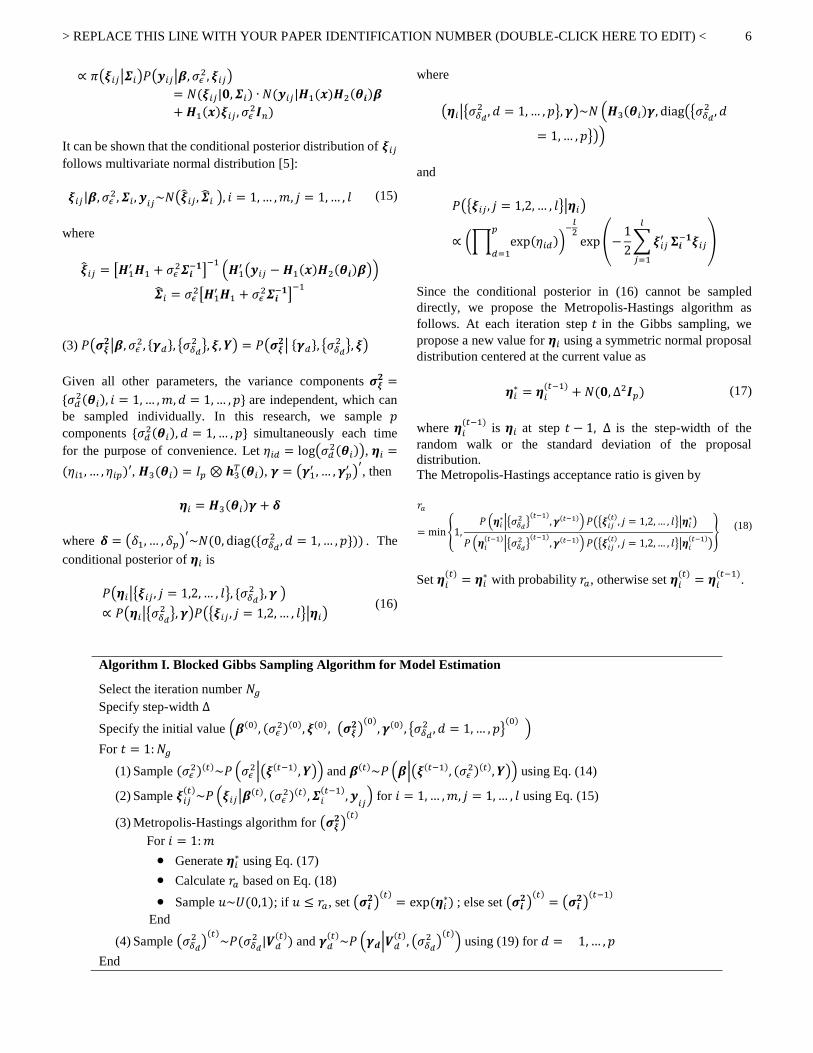
Since the conditional posterior in (16) cannot be sampled

directly, we propose the Metropolis-Hastings algorithm as

follows. At each iteration step 𝑡 in the Gibbs sampling, we

propose a new value for 𝜼𝑖 using a symmetric normal proposal

distribution centered at the current value as

𝜼𝑖∗ = 𝜼𝑖

(𝑡−1)+ 𝑁(𝟎, ∆2𝑰𝑝) (17)

where 𝜼𝑖(𝑡−1)

is 𝜼𝑖 at step 𝑡 − 1, ∆ is the step-width of the

random walk or the standard deviation of the proposal

distribution.

The Metropolis-Hastings acceptance ratio is given by

𝑟𝑎

= min{1,𝑃 (𝜼𝑖

∗|{𝜎𝛿𝑑2 }(𝑡−1), 𝜸(𝑡−1)) 𝑃({𝝃𝑖𝑗

(𝑡), 𝑗 = 1,2,… , 𝑙}|𝜼𝑖∗)

𝑃 (𝜼𝑖(𝑡−1)|{𝜎𝛿𝑑

2 }(𝑡−1), 𝜸(𝑡−1)) 𝑃({𝝃𝑖𝑗

(𝑡), 𝑗 = 1,2,… , 𝑙}|𝜼𝑖(𝑡−1))}

(18)

Set 𝜼𝑖(𝑡)= 𝜼𝑖

∗ with probability 𝑟𝑎, otherwise set 𝜼𝑖(𝑡)= 𝜼𝑖

(𝑡−1).

Algorithm I. Blocked Gibbs Sampling Algorithm for Model Estimation

Select the iteration number 𝑁𝑔

Specify step-width Δ

Specify the initial value (𝜷(0), (𝜎𝜖2)(0), 𝝃(0), (𝝈𝝃

𝟐)(0), 𝜸(0), {𝜎𝛿𝑑

2 , 𝑑 = 1,… , 𝑝}(0) )

For 𝑡 = 1:𝑁𝑔

(1) Sample (𝜎𝜖2)(𝑡)~𝑃 (𝜎𝜖

2|(𝝃(𝑡−1), 𝒀)) and 𝜷(𝑡)~𝑃 (𝜷|(𝝃(𝑡−1), (𝜎𝜖2)(𝑡), 𝒀)) using Eq. (14)

(2) Sample 𝝃𝑖𝑗(𝑡)~𝑃 (𝝃𝑖𝑗|𝜷

(𝑡), (𝜎𝜖2)(𝑡), 𝜮𝑖

(𝑡−1), 𝒚𝑖𝑗) for 𝑖 = 1, … ,𝑚, 𝑗 = 1,… , 𝑙 using Eq. (15)

(3) Metropolis-Hastings algorithm for (𝝈𝝃𝟐)(𝑡)

For 𝑖 = 1:𝑚

Generate 𝜼𝑖∗ using Eq. (17)

Calculate 𝑟𝑎 based on Eq. (18)

Sample 𝑢~𝑈(0,1); if 𝑢 ≤ 𝑟𝑎, set (𝝈𝒊𝟐)(𝑡)= exp(𝜼𝑖

∗) ; else set (𝝈𝒊𝟐)(𝑡)= (𝝈𝒊

𝟐)(𝑡−1)

End

(4) Sample (𝜎𝛿𝑑2 )(𝑡)~𝑃(𝜎𝛿𝑑

2 |𝑽𝑑(𝑡)) and 𝜸𝑑

(𝑡)~𝑃 (𝜸𝒅|𝑽𝑑(𝑡), (𝜎𝛿𝑑

2 )(𝑡)) using (19) for 𝑑 = 1, … , 𝑝

End


7

(4) 𝑃({𝜸𝑑}, {𝜎𝛿𝑑2 }|𝜷, 𝜎𝜖

2, 𝝈𝝃𝟐, 𝝃, 𝒀) = 𝑃({𝜸𝑑}, {𝜎𝛿𝑑

2 }| 𝝈𝝃𝟐)

Since (𝜸𝑑, 𝜎𝛿𝑑2 ) is independent of (𝜸𝑑′ , 𝜎𝛿𝑑′

2 ) for 𝑑 ≠ 𝑑′ , the

joint conditional posterior distribution of (𝜸𝑑 , 𝜎𝛿𝑑2 ), which is

similar to (14), can be sampled individually. Let 𝑽𝑑 =(log 𝜎𝑑

2(𝜽1) , … , log 𝜎𝑑2(𝜽 ))

′, 𝑯4 is the stack of {𝒉3(𝜽𝒊)𝑇 , 𝑖 =

1, … ,𝑚} , then similar to (14), the conditional posterior

distributions follow the distribution as

𝜎𝛿𝑑2 |𝑽𝑑~𝐼𝐺 (

𝑚 − 2

2,(𝑽𝒅 −𝑯𝟒��𝑑)

′(𝑽𝒅 −𝑯𝟒��𝑑)

2)

𝜸𝒅|𝑽𝑑 , 𝜎𝛿𝑑2 ~𝑁(��𝑑 , 𝜎𝛿𝑑

2 (𝑯4′𝑯4)

−𝟏)

(19)

where

��𝑑 = (𝑯4′𝑯4)

−1𝑯4′ 𝑽𝑑

The overall blocked Gibbs sampling is shown in the

Algorithm I. To speed up the convergence efficiency, the initial

value for all the models parameters can be set using

multiple-stage analysis, i.e., fitting linear regression for each

profile and treat each coefficient as response in the level-2

model fitting, and then use the sample residual variance of

level-2 model as the responses in the variance regression. After

the iteration of the Gibbs sampling is finished, the obtained

samples can be truncated to remove the initial bias for the

posterior estimation.

IV. MODEL SELECTION AND MICROSTRUCTURAL PARAMETER

INFERENCE

A. Model Selection using Intrinsic Bayes Factor

The most popular model selection methods are the

information criteria based methods, such as Akaike

Information Criteria (AIC; [29]) and Bayesian Information

Criteria (BIC; [30]), where the criteria is to find a model that

minimizes an estimate of a criterion consisting of a loss

function (e. g. , −2 × log-likelihood) and a penalty function.

These methods are commonly used in linear regressions, where

the penalty function is a function of model complexity, or

number of parameters. However, for the model proposed here,

there are both regression parameters and variance parameters at

different levels, which have different relative importance in

analysis. It is very challenging to incorporate the relative

importance into the penalty function of the information criteria.

The Bayes factor (BF) is a very flexible model selection

method that can compare models of any forms [31]. For two

competing models 𝑀𝑖 and 𝑀j , 𝑖 ≠ 𝑗 , the BF of 𝑀𝑖 to 𝑀𝑗 is

defined as the ratio of the observed marginal densities

𝐵𝑖𝑗 =𝑃(𝒀|𝑀𝑖)

𝑃(𝒀|𝑀𝑗)=∫𝑃(𝒀|𝝍𝒊, 𝑀𝑖)𝜋(𝝍𝒊|𝑀𝑖)𝑑𝝍𝒊

∫𝑃(𝒀|𝝍𝒋, 𝑀𝑗)𝜋(𝝍𝒋|𝑀𝑗)𝑑𝝍𝒋 (20)

where 𝑃(𝒀|𝑀𝑖) is the marginal or predictive densities of 𝒀, 𝝍𝒊 is the vector of model parameters and 𝜋(𝝍𝒊|𝑀𝑖) is the prior

density function of model parameters under model 𝑀𝑖. It can

also interpreted as the weighted likelihood ratio of 𝑀𝑖 to 𝑀𝑗,

with the priors being the “weighting functions”. Intuitively,

higher 𝐵𝑖𝑗 indicates a stronger evidence of 𝑀𝑖 against 𝑀𝑗. A set

of cutoff values of 𝐵𝑖𝑗 has been suggested and widely used in

literature [9, 32], as shown in Table I.

TABLE I

RANGE OF BF VALUES AND ITS EVIDENCE IN FAVOR OF 𝑴𝒊

𝑩𝒊𝒋 𝟐 𝐥𝐨𝐠(𝑩𝒊𝒋) Evidence against 𝑀𝑗

1~3 0~2 Barely worth mentioning

3~20 2~6 Positive

20~150 6~10 Strong

>150 >10 Very strong

Although BF is very flexible, a direct computation is very

challenging, since the marginal density involves integration

over the parameter space of high dimension. A natural

approach to solve this issue is MCMC simulation, where two

popular methods are used, the product space search and the

marginal likelihood estimation method [33]. When the two

models have parameters of different dimensions, however,

using improper noninformative priors for all models parameters

will result in indeterminate BFs, as the marginal density

𝑃(𝒀|𝑀𝑖) = ∫𝑃(𝒀|𝝍𝒊, 𝑀𝑖)𝜋(𝝍𝒊|𝑀𝑖)𝑑𝝍𝒊 is not well-defined

for 𝜋(𝝍𝒊|𝑀𝑖) ∝ 1 . To see how this happens, suppose

𝜋(𝝍𝒊|𝑀𝑖) ∝ 1 and 𝜋(𝝍𝒋|𝑀𝑗) ∝ 1 are used as priors for 𝑀𝑖 and

𝑀𝑗 respectively. Then 𝑐𝑖𝜋(𝝍𝒊|𝑀𝑖) and 𝑐𝑗𝜋(𝝍𝒋|𝑀𝑗) can also be

used as improper priors, which results in another BF 𝑐𝑖/𝑐𝑗𝐵𝑖𝑗.

In this paper, we propose to use the intrinsic Bayes factor (IBF)

[34] for model selection.

Let 𝒀(𝑠) denote the training profiles and 𝒀(−𝑠) denote the

remaining profiles for testing (the partition is based on the

value 𝜽 or based on the specimen). The basic idea of IBF is to

use the training profiles 𝒀(𝑠) to convert the improper

noninformative priors to proper posterior distributions and then

to compute the BF with the remainder of the profiles 𝒀(−𝑠). The IBF can be expressed as

𝐼𝐵𝑖𝑗 =𝑃(𝒀(−𝑠)|𝒀(𝑠),𝑀𝑖)

𝑃(𝒀(−𝑠)|𝒀(𝑠),𝑀𝑗)

=∫𝑃(𝒀(−𝑠)|𝝍𝒊)𝜋(𝝍𝒊|𝒀(𝑠))𝑑𝝍𝒊

∫𝑃(𝒀(−𝑠)|𝝍𝒋)𝜋(𝝍𝒋|𝒀(𝑠))𝑑𝝍𝒋

(21)

As we can see, the marginal density in IBF is quite similar to

cross-validation techniques commonly used in the model

validation. Naturally, we can partition all the profiles into

several groups and calculate the IBF using each group of

profiles as the testing profiles and the remainder as the training

profiles. By averaging all the IBFs, we can get a more stable

IBF.

Although the marginal density is well-defined with proper

posterior distribution 𝜋(𝝍𝒊|𝒀(𝑠)) , the direct computation is

still challenging. With the availability of posterior samples of

𝜋(𝝍𝒊|𝒀(𝑠)) obtained from the blocked Gibbs sampler, we can

compute the IBF using MCMC approach as follows. The

marginal density for 𝑀𝑖 is written as


8

𝑚𝑖(𝒀(−𝑠)|𝒀(𝑠)) =

∫𝑓(𝒀(−𝑠)|𝝍𝑖 , (𝝈𝝃𝟐(−𝑠))𝑖)𝜋((𝝈𝝃

𝟐(−𝑠))𝑖|𝝍𝑖)𝜋(𝝍𝑖|𝒀(𝑠))𝑑(𝝍𝑖 , (𝝈𝝃𝟐(−𝑠))𝑖)

Here (𝝈𝝃𝟐(−𝑠))𝑖 denote the variances of random effects of the

testing profiles 𝒀(−𝑠) under the mode 𝑀𝑖 . Suppose the

posterior samples of the training data 𝒀(𝑠) obtained in the

Gibbs sampling are

{(𝝍𝑖(𝑔), 𝝃(𝑠)𝑖

(𝑔), (𝝈𝝃

𝟐(𝑠))𝑖

(𝑔)

) , 𝑔 = 1,2, … , 𝐺 }

Then for 𝑔 = 1,… , 𝐺, we can sample (𝝈𝝃𝟐(−𝑠))

(𝑔)conditioning

on 𝝍(𝑔) through the lognormal distribution, as shown in (5).

The marginal density could be estimated by

𝑚𝑖(𝒀(−𝑠)|𝒀(𝑠))

≈1

𝐺∑𝑓 (𝒀(−𝑠)|𝝍𝑖

(𝑔), (𝝈𝝃

𝟐(−𝑠))𝑖

(𝑔)

)

𝐺

𝑔=1

(22)

where the profile 𝒚(𝜽) given 𝝍 and 𝝈𝝃𝟐 follows normal

distribution based on (4):

𝒚(𝜽) |𝝍, 𝚺𝛏(𝜽)~𝑵(𝑯1(𝒙)𝑯2(𝜽)𝜷,𝑯1(𝒙)𝚺𝛏(𝜽)𝑯1(𝒙)′ + 𝜎𝜖

2𝑰)

B. Inference on the Microstructural Parameter

After the optimal model is selected and estimated through

the Gibbs sampler and IBF, we can use it to infer the

microstructural parameters 𝜽 for quality control and diagnosis.

Suppose the measured profiles for a new specimen are 𝒀𝑛𝑒𝑤,

then the posterior of 𝜽𝑛𝑒𝑤 given 𝒀𝑛𝑒𝑤 and model parameters is

of interest. If we use the mean or median of the posterior

distributions of 𝝍 as the point estimate of the model

parameters, denoted as �� , then the posterior of 𝜽𝑛𝑒𝑤 is

𝑃(𝜽𝑛𝑒𝑤|𝒀𝑛𝑒𝑤 , ��). Alternatively, we could use all the Gibbs

samples instead of the point estimate for the model parameters.

Algorithm II. Inference of 𝜽 using Importance Sampling

Specify the number of samples 𝑁𝑠

(1) Draw samples 𝜽(1), … , 𝜽(𝑁𝑠)from 𝜋(𝜽𝑛𝑒𝑤) (2) Calculate the importance weight of each sample using

(22)

𝑤(𝑗) = 𝑃(𝒀𝑛𝑒𝑤|𝜽(𝑗) , 𝒀), 𝑗 = 1,… , 𝑁𝑠

(3) Approximate the expectation

𝐸𝑃(𝜽|𝒀𝑛𝑒𝑤 , 𝒀)(ℎ(𝜽)) =

∑ 𝑤(𝑗)ℎ(𝜽(𝑗))𝑁𝑠𝑗=1

∑ 𝑤(𝑗)𝑁𝑠𝑗=1

The posterior is expresses as

𝑃(𝜽𝑛𝑒𝑤|𝒀𝑛𝑒𝑤 , 𝒀) ∝ 𝜋(𝜽𝑛𝑒𝑤)𝑃(𝒀𝑛𝑒𝑤|𝜽𝑛𝑒𝑤 , 𝒀) (23)

where 𝜋(𝜽𝑛𝑒𝑤) is the prior distribution for 𝜽. To estimate this

posterior, the importance sampling [35] can be applied where

the prior 𝜋(𝜽𝑛𝑒𝑤) is selected as the importance distribution

and 𝑃(𝒀𝑛𝑒𝑤|𝜽𝑛𝑒𝑤 , 𝒀) is the weight function, which can be

estimated using (22). The expectation of ℎ(𝜽𝑛𝑒𝑤) with respect

to 𝑃(𝜽𝑛𝑒𝑤|𝒀𝑛𝑒𝑤 , 𝒀) where ℎ(𝜽𝑛𝑒𝑤) is any function of 𝜽𝑛𝑒𝑤 ,

can be estimated using the Algorithm II.

V. NUMERICAL STUDY FOR PERFORMANCE EVALUATION

In this section, simulated profiles are used to evaluate the

efficiency of the proposed Gibbs sampling for model

estimation, intrinsic Bayes factor for model selection, and

parameter inference. In total two models are used in the

simulation, with one model for illustration of posterior

sampling and both models for model selection and parameter

inference.

A. Simulation Setup

The models used in the simulation with specified parameters

are shown in Table II. For simplicity we assume that 𝜃 is a

scalar parameter and ℎ𝑖(∙), 𝑖 = 1,2,3 are polynomials of

degrees 𝑝 − 1, 𝑞 − 1 and 𝑟 − 1 respectively.

TABLE II

MODEL SETTING FOR SIMULATION

Model 1 Model 2

𝑝 = 2, 𝑞 = 3, 𝑟 = 2

ℎ1(𝑥) = (𝑥, 1)′

ℎ2(𝜃) = (𝜃2, 𝜃, 1)′

ℎ3(𝜃) = (𝜃, 1)′

𝜷1 = (2,2,2)′, 𝜷2 = (−1,−1,−1)

′

𝜸1 = (6,−6)′, 𝜸2 = (4,−4)

′

𝜎𝜖2 = 0.01, 𝜎𝛿1

2 = 𝜎𝛿22 = 0.1

𝑝 = 2, 𝑞 = 2, 𝑟 = 2

ℎ1(𝑥) = (𝑥, 1)′

ℎ2(𝜃) = (𝜃, 1)′

ℎ3(𝜃) = (𝜃, 1)′

𝜷1 = (2,4)′, 𝜷2 = (−1,3)

′

𝜸1 = (4,−5)′, 𝜸2 = (6,−7)

′

𝜎𝜖2 = 0.01, 𝜎𝛿1

2 = 𝜎𝛿22 = 0.01

Fig. 3. Illustration of the simulated profiles from Model 1 with increasing 𝜃

from 0.1 to 0.9: (a), (b),… , (i) corresponds to 𝜃 = 0.1,0.2,… , 0.9 respectively.

For each model, 𝑙 = 60 profiles are generated with 𝑚 = 33

equally spaced design points for 𝜃 in [0.1, 0.9], i.e., 𝜃 =


9

0.1,0.125, … ,0.9, and 𝑛 = 11 equally spaced design points for

𝑥 in [2, 3], i.e., 𝑥 = 2, 2.1, … ,3. The first model will be used to

show the efficiency of blocked Gibbs sampling and both

models will be used to illustrate the IBF model selection and

parameter inferences. Fig. 3 shows part of the simulated

profiles from Model 1, where we can see obvious increase of

between-curve dispersion when increasing 𝜃.

B. Results of Posterior Sampling

In the posterior sampling, we assume that the true model of

the simulated profiles is given. Only the model parameters are

unknown and need to be estimated. The initial values for all

parameters are arbitrarily set to 1. The standard deviation of the

proposal distribution is set as ∆= 0.1.

Fig. 4. Sample paths of several representative mean and variance parameters

from blocked Gibbs sampling; the horizontal dashed lines denote the true

parameters of the model.

Fig. 5. Histograms of the parameter samples; the vertical dashed lines denote

the true parameters

Fig. 4 shows the sample paths of several representative mean

and variance parameters of Model 1. As we can see, all the

chains gradually move into the true values of the model

parameters after about 20K iterations. We can also observe that

the sequences of samples are highly correlated, i.e., requiring

many iterations to forget the starting point and reach the

equilibrium distribution. The step-width ∆ could be increased

or adjusted to reduce the correlation and speed up the

convergence. Since it is not the focus, we will not discuss it

here. The total computational time of the Gibbs sampling step is

about 12 minutes using MATLAB running on an Intel core

i5-4590 processor of 3.3GHz. The histograms of the samples in

the equilibrium stage are shown in Fig. 5, where the last 10K

samples of each chain are selected. As we can see, the centers

of the posterior are very close to the true values.

C. Model Selection

Changing the degree of the polynomial in each submodel, or

setting certain coefficients to zero with fixed degree at each

level, will result in many candidate models, which makes it

unrealistic to fit all models and compare them all. In

application, the multiple-stage analysis (i.e., fitting the model

from the first level to the last one, and using fitted parameters in

current level as responses in the next level fitting) can be used

to select some most likely models and then use IBF to select the

best one among them. Alternatively, the forward selection

strategy can be used, where one starts from the simplest model,

and each time adds one variable that has the most significant

improvement (i.e., increase in marginal density) to the model

fitting until there is no significant improvement. For simplicity,

we only compare models with different degrees to illustrate the

effectiveness of IBF in model selection. In the IBF

computation, the profiles with 𝜃 = 0.1,0.125, … 0.725 are

used as training data and others with 𝜃 = 0.75, 0.775, … ,0.9

are used as testing data.

TABLE III

CANDIDATE MODELS, MARGINAL DENSITIES AND THE IBF OF THE TRUE

MODELS TO OTHERS

Model Dim.

(𝑝, 𝑞, 𝑟)

Data1 Data2

log(𝑚𝑖) 2 log(𝐼𝐵𝐹) log(𝑚𝑖) 2 log(𝐼𝐵𝐹)

𝑀1 (2,1,1) 17.3 221.2 92.7 111.2

𝑀2 (2,1,2) 67.6 120.6 108.6 79.4

𝑀3 (2,1,3) 58.5 138.8 101.3 94

𝑀4 (2,2,1) 100.8 54.2 141.4 13.8

𝑀5 (2,2,2) 123.9 8 148.3 −

𝑀6 (2,2,3) 123.1 9.6 126.6 43.4

𝑀7 (2,3,1) 105.9 44 140.0 16.6

𝑀8 (2,3,2) 127.9 − 148.2 0.2

𝑀9 (2,3,3) 127.5 0.8 147.1 2.4

𝑀10 (3,1,1) 46.0 163.8 45.7 205.2

𝑀11 (3,1,2) 38.9 178.0 52.3 192

𝑀12 (3,1,3) 26.5 202.8 41.9 212.8

𝑀13 (3,2,1) 53.3 149.2 65.2 166.2

𝑀14 (3,2,2) 64.5 126.8 64.6 167.4

𝑀15 (3,2,3) 45.4 165 59.9 176.8

𝑀16 (3,3,1) 48.9 158 67.5 161.6

𝑀17 (3,3,2) 72.8 110.2 67.5 161.6

𝑀18 (3,3,3) 53.3 149.2 62.2 172.2

Table III shows the candidate models, estimated marginal

densities and the IBF for the two set of profile data (Data1 and

Data2) generated from Model 1 and Model 2. As we can see,

the true models for both dataset, i.e., 𝑀8 for Data1 and 𝑀5 for


10

Data2, have the highest marginal densities than all other

candidate models. Almost all the IBFs of the true models to

other candidate models are significant according to the

recommended BF range and evidence given in Table I. Note

that the IBF of 𝑀8 to 𝑀9 for Data1 and the IBF of 𝑀5 to 𝑀8 for

Data2 are not significant in terms of the IBF value. However,

𝑀8 is simpler than 𝑀9 and 𝑀5 is simpler than 𝑀8, indicating

that the true models 𝑀8 and 𝑀5 are preferable to 𝑀9 and 𝑀8 for Data1 and Data2 respectively. Therefore, the IBF can

effectively select the best model among all candidate models.

D. Inference of the Microstructural Parameter 𝜃

𝜃 = 0.4, 0.6, 0.8 are used to generate the new data using

Model 1 and Model 2 for parameter inference. 20 profiles are

generated for each 𝜃. The prior distribution of 𝜃 is assumed to

be uniform in the interval [0,1]. The posterior distribution of 𝜃

is estimated using the importance sampling algorithm shown in

Section 4.3.

Fig. 6. Estimated posterior distribution of 𝜽: (a)-(c) for Model 1 and (d)-(f) for

Model 2. The vertical dashed lines denote the true 𝜽.

Fig. 6 shows the estimated posterior distributions. We can

see that the center of the posterior is very close to the true value

of 𝜃, and the variance of the posterior using 20 profiles is also

very small. The computational cost of the posterior estimation

is about 26 minutes for total 40 samples using MATLAB under

the same computer configuration as used in Section B. The

computational burden may be an issue in online applications

where faster inference is required. To overcome this issue,

parallel computing could be applied to speed up the

computation.

VI. APPLICATION TO ULTRASONIC ATTENUATION PROFILES IN

NANOCOMPOSITES MANUFACTURING

In this section the proposed model is applied to the ultrasonic

attenuation profiles of the A206-Al2O3 nanocomposites for

quality inspection. Due to high experimental cost and difficulty

in fabricating nanocomposites of desired microstructural

features, it is very challenging to obtain sufficient experimental

data for model building. Liu et al [8] recently proposed a

microstructural modeling and wave propagation simulation

approach to enrich the database of microstructures and the

corresponding ultrasonic attenuation profiles. A Voronoi

diagram is modified to simulate the microstructures based on

the micrographs and morphology modification mechanisms of

Al2O3 nanoparticles, and then an elastodynamic finite

integration technique VEFIT[36] is used to simulate the wave

propagation. In the simulation, the attenuation profiles are

measured at a fixed location of repeatedly simulated specimens,

which is equivalent to measuring different locations of one

specimen. The simulation approach can effectively capture the

features of microstructures and generate attenuation profiles

comparable to experimental results. In the microstructure

generation, two key parameters are used to control the

morphology, the number of cells 𝑁 , and the percentage of

Voronoi edge length left after dissolving, denoted as 𝜃.

Fig. 7. Attenuation profiles for microstructures with 𝜃 = (0.1,0.2,… ,0.9) from

(a) to (i).

Fig. 8. Exploratory analysis for the attenuation profiles using multiple-stage

analysis. The solid lines denote the simple linear regression lines.


11

Fig. 7 shows the attenuation profiles (20 profiles each

sub-figure) of microstructures with 𝜃 = (0.1,0.2, … ,0.9) and

the corresponding 𝑁′𝑠 that keeps the total amount of

intermetallic phase unchanged. As we can see, the attenuation

profiles linearly increase with frequency in the selected

frequency range, and the between-profile variation increases

with 𝜃. Fig. 8 shows the exploratory analysis of the attenuation

profiles using the multiple-stage analysis. We can see that the

slope, intercept and their log-variances are quite linear with 𝜃.

The model selection is conducted to the data and the optimal

model with 𝑝 = 2, 𝑞 = 2 and 𝑟 = 2 is selected. The estimated

parameters using the mean of the posterior samples are 𝛽11 =0.231, 𝛽12 = 0.253, 𝛽21 = −0.489, 𝛽22 = −0.396 , 𝜎𝜖

2 =4.95 × 10−4 , 𝛾11 = 9.92 , 𝛾12 = −12.72 , 𝛾21 = 11.31 ,

𝛾22 = −12.68, 𝜎𝛿12 = 0.0077 and 𝜎𝛿2

2 = 0.01.

Fig. 9. Posterior distribution of 𝜃 for (a): Simulated attenuation with 𝜃 = 0.2; (b) simulated attenuation with 𝜃 = 0.8 ; (c) A206+1wt%Al2O3, and (d):

A206+5wt%Al2O3. The vertical dashed lines denote the true 𝜃.

The estimated model is used to infer the microstructural

parameters of two physically simulated microstructures (𝜃 =0.2 and 0.8). Fig. 9 (a) and (b) show the posterior distribution

of 𝜃 with uniform prior distribution 𝑈(0,1). We can clearly see

that the posteriors are centered on the true values with small

variance. The established model is also applied to two

fabricated specimens with attenuation profiles shown in Fig. 1.

For the two specimens, the posteriors of 𝜃 are shown in Fig. 9

(c) and (d), respectively. The mean estimates of the posteriors

are 0.68 and 0.46 respectively. We can see that the 𝜃 of first

specimen is higher than the second one, which is consistent

with the experimental result that the second specimen has

smaller grain size and more homogeneous microstructure. By

setting a threshold 𝜃0 for 𝜃 , the posterior can be used to

estimate the probability of 𝜃 < 𝜃0 and use it to for quality

control. Therefore the estimated posterior distribution can be

used for both quality control and microstructure diagnosis in

the ultrasonic attenuation based quality inspection of

nanocomposites.

We also fitted a standard Bayesian HLM without considering

the variance heterogeneity, i.e., the covariance matrix is

constant across all microstructural parameters. For page limits,

we do not put the detailed results here. We found that the

estimated parameters of 𝜷 and 𝜎𝜖2 are very close between these

two models. However, the diagonal entries of the estimated

covariance matrix �� are higher than those of the proposed

model for 𝜃 < 0.7 , and lower for 𝜃 > 0.7 . It is what we

expected since the estimated variance in the model with

constant variance has to compromise between large

between-profile variance and small between-profile variance.

In the microstructural parameter inference, the posterior modes

are very close between these two models. However, the

variance of the posterior distribution for the model without

considering variance heterogeneity is significantly higher than

the proposed model, indicating that the inference using the

former is not as informative as using the latter. The addition of

the variance heterogeneity model provides more information in

the microstructural parameter inference and thus leads to a

more accurate inference. This advantage would be more

significant when 𝜷 is not sensitive to 𝜃. An extreme case is that

𝜷 is constant across all design points 𝜃𝑖 while only 𝜮 varies

with 𝜃 . In such case, the model without considering the

between-profile variance is not able to infer the microstructural

parameter anymore.

VII. CONCLUSION AND DISCUSSION

In this paper, a hierarchical linear model with level-2

variance heterogeneity is proposed to build a relationship

between profiles data, the explanatory variables, and the

microstructural parameters for quality inspection and control.

The integrated Bayesian framework for model estimation and

selection is proposed through the blocked Gibbs sampling and

intrinsic Bayes factor. The inference of the microstructural

parameters based on the estimated model is proposed through

importance sampling. The numerical study shows that the

proposed approach can effectively identify the true model,

estimate the model parameters, and infer the microstructural

parameters for new profiles. The proposed model is applied to

the ultrasonic attenuation profiles in the manufacturing of

metal-matrix nanocomposites. The results show that this

approach can be effectively used for quality inference and

control. Compared with standard hierarchical linear model, the

addition of the variance heterogeneity provides more

information in microstructural parameter inference and thus

give more accurate inference.

There may still exist other issues that need to be addressed to

make this model more robust in many applications. One issue is

that if the profile is very complex in shape, e.g. tonnage signals

in [37], simple linear model is not adequate to characterize each

profile. We may need nonparametric nonlinear models, such as

wavelets or B-splines in regression. Another typical issue we

may face is the “curse of dimensionality”. If the dimension of

the model is very high, it may require a large amount of

historical profile data in model building. Besides, to select an

appropriate model, it may need to compare a large number of

candidate models (e.g., degree of polynomial is very high),


12

which is often unrealistic. One possible solution to this issue is

to incorporate domain knowledge or physical models into

statistical models to simplify the selection process.

REFERENCES

[1] X. Li, Y. Yang, and D. Weiss, "Ultrasonic Cavitation Based Dispersion of Nanoparticles in Aluminum Melts for Solidification Processing of

Bulk Aluminum Matrix Nanocomposite: Theoretical Study, Fabrication

and Characterization," 2007. [2] J. Wu, Li, Xiaochun, Zhou, Shiyu, "Acoustic Emission Monitoring for

Ultrasonic Cavitation Based Dispersion Process," Journal of

Manufacturing Science and Engineering, 2013. [3] H. Choi, W.-h. Cho, H. Konishi, S. Kou, and X. Li,

"Nanoparticle-Induced Superior Hot Tearing Resistance of A206 Alloy,"

Metallurgical and Materials Transactions A, pp. 1-11, 2013. [4] Y. Yang and X. Li, "Ultrasonic cavitation-based nanomanufacturing of

bulk aluminum matrix nanocomposites," Journal of Manufacturing

Science and Engineering, vol. 129, pp. 252-255, 2007.

[5] J. Wu, Chen, Yong, Li, Xiaochun, Zhou, Shiyu, "Online Steady-state

Detection for Process Control Using Multiple Change-point Models and

Particle Filters," IEEE Transactions on Automation Science and Engineering, 2015.

[6] J. Wu, S. Zhou, and X. Li, "Ultrasonic Attenuation Based Inspection

Method for Scale-up Production of A206–Al2O3 Metal Matrix Nanocomposites," Journal of manufacturing science and engineering,

vol. 137, p. 011013, 2015. [7] F. M. Sears and B. P. Bonner, "Ultrasonic attenuation measurement by

spectral ratios utilizing signal processing techniques," Geoscience and

Remote Sensing, IEEE Transactions on, pp. 95-99, 1981. [8] Y. Liu, J. Wu, S. Zhou, and X. Li, "Microstructure Modelling and

Ultrasonic Wave Propagation Simulation of A206-Al2O3 Metal Matrix

Nanocomposites for Quality Inspection," Journal of manufacturing science and engineering, 2015.

[9] L. Zeng and N. Chen, "Bayesian hierarchical modeling for monitoring

optical profiles in low-E glass manufacturing processes," IIE Transactions, vol. 47, pp. 109-124, 2015.

[10] W. H. Woodall, "Current research on profile monitoring," Production,

vol. 17, pp. 420-425, 2007. [11] R. Noorossana, A. Saghaei, and A. Amiri, Statistical analysis of profile

monitoring vol. 865: John Wiley & Sons, 2011.

[12] W. H. Woodall, D. J. Spitzner, D. C. Montgomery, and S. Gupta, "Using control charts to monitor process and product quality profiles," Journal of

Quality Technology, vol. 36, pp. 309-320, 2004.

[13] W. A. Jensen, J. B. Birch, and W. H. Woodall, "Monitoring correlation within linear profiles using mixed models," Journal of Quality

Technology, vol. 40, pp. 167-183, 2008.

[14] S. W. Raudenbush and A. S. Bryk, Hierarchical linear models: Applications and data analysis methods vol. 1: Sage, 2002.

[15] H. Goldstein, Multilevel statistical models vol. 922: John Wiley & Sons,

2011. [16] X. Lin, J. Raz, and S. D. Harlow, "Linear mixed models with

heterogeneous within-cluster variances," Biometrics, pp. 910-923, 1997.

[17] J. L. Foulley and R. Quaas, "Heterogeneous variances in Gaussian linear mixed models," Genetics Selection Evolution, vol. 27, pp. 211-228, 1995.

[18] H. Zheng, Y. Yang, and K. C. Land, "Variance Function Regression in

Hierarchical Age-Period-Cohort Models Applications to the Study of Self-Reported Health," American sociological review, vol. 76, pp.

955-983, 2011.

[19] J. C. Pinheiro and D. M. Bates, Mixed-effects models in S and S-PLUS: Springer Science & Business Media, 2000.

[20] G. K. Smyth, A. F. Huele, and A. P. Verbyla, "Exact and approximate

REML for heteroscedastic regression," Statistical modelling, vol. 1, pp. 161-175, 2001.

[21] M. Davidian and R. J. Carroll, "Variance function estimation," Journal of

the American statistical association, vol. 82, pp. 1079-1091, 1987. [22] Y. Fan and R. Li, "Variable selection in linear mixed effects models,"

Annals of statistics, vol. 40, p. 2043, 2012.

[23] E. Del Castillo, B. M. Colosimo, and H. Alshraideh, "Bayesian modeling and optimization of functional responses affected by noise factors,"

Journal of Quality Technology, vol. 44, p. 117, 2012.

[24] A. Gelman, J. B. Carlin, H. S. Stern, and D. B. Rubin, Bayesian data

analysis vol. 2: Taylor & Francis, 2014. [25] J. P. Hobert and G. Casella, "The effect of improper priors on Gibbs

sampling in hierarchical linear mixed models," Journal of the American

statistical association, vol. 91, pp. 1461-1473, 1996. [26] A. Gelman, "Prior distributions for variance parameters in hierarchical

models (comment on article by Browne and Draper)," Bayesian analysis,

vol. 1, pp. 515-534, 2006. [27] J. S. Liu, W. H. Wong, and A. Kong, "Covariance structure of the Gibbs

sampler with applications to the comparisons of estimators and

augmentation schemes," Biometrika, vol. 81, pp. 27-40, 1994. [28] S. Chib and E. Greenberg, "Understanding the metropolis-hastings

algorithm," The american statistician, vol. 49, pp. 327-335, 1995.

[29] H. Akaike, "Information theory and an extension of the maximum likelihood principle," in Selected Papers of Hirotugu Akaike, ed:

Springer, 1998, pp. 199-213.

[30] G. Schwarz, "Estimating the dimension of a model," The Annals of Statistics, vol. 6, pp. 461-464, 1978.

[31] J. O. Berger, L. R. Pericchi, J. Ghosh, T. Samanta, F. De Santis, J. Berger,

and L. Pericchi, "Objective Bayesian methods for model selection: introduction and comparison," Lecture Notes-Monograph Series, pp.

135-207, 2001.

[32] R. E. Kass and A. E. Raftery, "Bayes factors," Journal of the American statistical association, vol. 90, pp. 773-795, 1995.

[33] C. Han and B. P. Carlin, "Markov chain Monte Carlo methods for

computing Bayes factors," Journal of the American statistical association, vol. 96, 2001.

[34] J. O. Berger and L. R. Pericchi, "The intrinsic Bayes factor for model selection and prediction," Journal of the American statistical association,

vol. 91, pp. 109-122, 1996.

[35] J. S. Liu, Monte Carlo strategies in scientific computing: springer, 2008. [36] C. Villagomez, L. Medina, and W. Pereira, "Open source acoustic wave

solver of elastodynamic equations for heterogeneous isotropic media," in

Ultrasonics Symposium (IUS), 2012 IEEE International, 2012, pp. 1521-1524.

[37] J. Jin and J. Shi, "Feature-preserving data compression of stamping

tonnage information using wavelets," Technometrics, vol. 41, pp. 327-339, 1999.

Jianguo Wu is an Assistant Professor in

the Department of Industrial,

Manufacturing and Systems Engineering

at University of Texas-El Paso, TX,

USA. He received the B.S. degree in

Mechanical Engineering from Tsinghua

University, Beijing, China in 2009, the

M.S. degree in Mechanical Engineering

from Purdue University, West Lafayette,

IN, USA in 2011, and M.S. degree in Statistics in 2014 and

Ph.D. degree in Industrial and Systems Engineering in 2015,

both from University of Wisconsin-Madison, Madison, WI,

USA. His research interests are focused on statistical modeling,

monitoring and analysis of complex processes/systems for

quality control and productivity improvement through

integrated application of metrology, engineering domain

knowledge and data analytics. He is a member of the Institute

for Operations Research and the Management Sciences

(INFORNS), the Institute of Industrial Engineers (IIE), the

Society of Manufacturing Engineers (SME).


13

Yuhang Liu received the B.S. degree in

mathematics in 2012 and the M.S. degree

in industrial and system engineering in

2013 from University of Minnesota Twin

Cities. He is currently a Ph.D. student in

University of Wisconsin Madison. He is a

member of the Institute for Operations

Research and the Management Science

(INFORMS) and SME.

Shiyu Zhou is a Professor in the

Department of Industrial and Systems

Engineering at the University of

Wisconsin-Madison. He received his B.S.

and M.S. in Mechanical Engineering from

the University of Science and Technology

of China in 1993 and 1996, respectively,

and his master’s in Industrial Engineering

and Ph.D. in Mechanical Engineering from

the University of Michigan in 2000. His research interests

include in-process quality and productivity improvement

methodologies by integrating statistics, system and control

theory, and engineering knowledge. He is a recipient of a

CAREER Award from the National Science Foundation and

the Best Application Paper Award from IIE Transactions. He is

a member of IIE, INFORMS, ASME, and SME.

Documents

Bayesian Hierarchical Linear Modeling of Profile Data with ...imse.utep.edu/mdasi/paper/paper8.pdf · Profile Data with Applications to Quality Control of Nanomanufacturing ... microstructural