Bayes’ Rule - Amazon S3s3.amazonaws.com/compressed.photo.goodreads.com/...Preface This introductory text is intended to provide a straightforward ex-planation of Bayes’ rule, using

Bayes’ RuleA Tutorial Introduction to Bayesian Analysis

James V Stone

Title:Bayes’ Rule: A Tutorial Introduction to Bayesian Analysis

Author: James V StonePublished by Sebtel Press

All rights reserved. No part of this book may be reproduced ortransmitted in any form or by any means, electronic or mechanical,including photocopying, recording or by any information storage andretrieval system, without written permission from the author.

First Edition, 2013.Typeset in LATEX2".

Cover Design by Stefan Brazzo.Copyright c�2013 by James V Stone

Fifth printing.

ISBN 978-0-9563728-4-0

To mum.

It is remarkable that a science which began with the con-sideration of games of chance should have become the mostimportant object of human knowledge.Pierre Simon Laplace, 1812.

Contents

Preface

1. An Introduction to Bayes’ Rule 11.1. Example 1: Poxy Diseases . . . . . . . . . . . . . . . . . 31.2. Example 2: Forkandles . . . . . . . . . . . . . . . . . . . 161.3. Example 3: Flipping Coins . . . . . . . . . . . . . . . . 211.4. Example 4: Light Craters . . . . . . . . . . . . . . . . . 251.5. Forward and Inverse Probability . . . . . . . . . . . . . 27

2. Bayes’ Rule in Pictures 292.1. Random Variables . . . . . . . . . . . . . . . . . . . . . 292.2. The Rules of Probability . . . . . . . . . . . . . . . . . . 312.3. Joint Probability and Coin Flips . . . . . . . . . . . . . 332.4. Probability As Geometric Area . . . . . . . . . . . . . . 342.5. Bayes’ Rule From Venn Diagrams . . . . . . . . . . . . . 412.6. Bayes’ Rule and the Medical Test . . . . . . . . . . . . 43

3. Discrete Parameter Values 473.1. Joint Probability Functions . . . . . . . . . . . . . . . . 483.2. Patient Questions . . . . . . . . . . . . . . . . . . . . . . 523.3. Deriving Bayes’ Rule . . . . . . . . . . . . . . . . . . . 653.4. Using Bayes’ Rule . . . . . . . . . . . . . . . . . . . . . 683.5. Bayes’ Rule and the Joint Distribution . . . . . . . . . . 70

4. Continuous Parameter Values 734.1. A Continuous Likelihood Function . . . . . . . . . . . . 734.2. A Binomial Prior . . . . . . . . . . . . . . . . . . . . . . 784.3. The Posterior . . . . . . . . . . . . . . . . . . . . . . . . 794.4. A Rational Basis For Bias . . . . . . . . . . . . . . . . . 814.5. The Uniform Prior . . . . . . . . . . . . . . . . . . . . . 814.6. Finding the MAP Analytically . . . . . . . . . . . . . . 854.7. Evolution of the Posterior . . . . . . . . . . . . . . . . . 874.8. Reference Priors . . . . . . . . . . . . . . . . . . . . . . 914.9. Loss Functions . . . . . . . . . . . . . . . . . . . . . . . 92

5. Gaussian Parameter Estimation 955.1. The Gaussian Distribution . . . . . . . . . . . . . . . . 955.2. Estimating the Population Mean . . . . . . . . . . . . . 975.3. Error Bars for Gaussian Distributions . . . . . . . . . . 1035.4. Regression as Parameter Estimation . . . . . . . . . . . 104

6. A Bird’s Eye View of Bayes’ Rule 1096.1. Joint Gaussian Distributions . . . . . . . . . . . . . . . 1096.2. A Bird’s-Eye View of the Joint Distribution . . . . . . 1126.3. A Bird’s-Eye View of Bayes’ Rule . . . . . . . . . . . . . 1156.4. Slicing Through Joint Distributions . . . . . . . . . . . . 1166.5. Statistical Independence . . . . . . . . . . . . . . . . . . 116

7. Bayesian Wars 1197.1. The Nature of Probability . . . . . . . . . . . . . . . . . 1197.2. Bayesian Wars . . . . . . . . . . . . . . . . . . . . . . . 1257.3. A Very Short History of Bayes’ Rule . . . . . . . . . . . 128

Further Reading 129

Appendices 131

A. Glossary 133

B. Mathematical Symbols 137

C. The Rules of Probability 141

D. Probability Density Functions 145

E. The Binomial Distribution 149

F. The Gaussian Distribution 153

G. Least-Squares Estimation 155

H. Reference Priors 157

I. MatLab Code 159

References 165

Index 169

Preface

This introductory text is intended to provide a straightforward ex-

planation of Bayes’ rule, using plausible and accessible examples. It is

written specifically for readers who have little mathematical experience,

but who are nevertheless willing to acquire the required mathematics

on a ‘need to know’ basis.

Lecturers (and authors) like to teach using a top-down approach,

so they usually begin with abstract general principles, and then move

on to more concrete examples. In contrast, students usually like to

learn using a bottom-up approach, so they like to begin with examples,

from which abstract general principles can then be derived. As this

book is not designed to teach lecturers or authors, it has been written

using a bottom-up approach. Accordingly, the first chapter contains

several accessible examples of how Bayes’ rule can be useful in everyday

situations, and these examples are examined in more detail in later

chapters. The reason for including many examples in this book is

that, whereas one reader may grasp the essentials of Bayes’ rule from

a medical example, another reader may feel more comfortable with the

idea of flipping a coin to find out if it is ‘fair’. One side-e↵ect of so many

examples is that the book may appear somewhat repetitive. For this,

I make no apology. As each example is largely self-contained, it can be

read in isolation. The obvious advantages of this approach inevitably

lead to a degree of repetition, but this is a small price to pay for the

clarity that an introductory text should possess.

MatLab and Python Computer Code

MatLab code listed in the appendices can be downloaded from

http://jim-stone.sta↵.shef.ac.uk/BookBayes2012/BayesRuleMatlabCode.html

Python code, which mirrors the MatLab code, is being developed at

the time of writing (3rd printing), and will be made available at

http://jim-stone.sta↵.shef.ac.uk/BookBayes2012/BayesRulePythonCode.html

Corrections

Please email any corrections to j.v.stone@she�eld.ac.uk. A list of cor-

rections is at http://jim-stone.sta↵.shef.ac.uk/BayesBook/Corrections.

Acknowledgments

Thanks to friends and colleagues for reading draft chapters, including

David Buckley, Nikki Hunkin, Danielle Matthews, Steve Snow, Tom

Sta↵ord, Stuart Wilson, Paul Warren, Charles Fox, and to John de

Pledge for suggesting the particular medical example in Section 2.6.

Special thanks to Royston Sellman for providing Python computer

code, which can be downloaded from the book’s website (see above).

Thanks to those readers who have emailed me to point out errors.

Finally, thanks to my wife, Nikki Hunkin, for sound advice on the

writing of this book, during which she tolerated Bayesian reasoning

being applied to almost every aspect of our lives.

Jim Stone,

She�eld, England,

December, 2014.

Chapter 1

An Introduction to Bayes’ Rule

“... we balance probabilities and choose the most likely. It

is the scientific use of the imagination ... ”

Sherlock Holmes, The Hound of the Baskervilles.

AC Doyle, 1901.

Introduction

Bayes’ rule is a rigorous method for interpreting evidence in the context

of previous experience or knowledge. It was discovered by Thomas

Bayes (c. 1701-1761), and independently discovered by Pierre-Simon

Laplace (1749-1827). After more than two centuries of controversy,

during which Bayesian methods have been both praised and pilloried,

Bayes’ rule has recently emerged as a powerful tool with a wide range

(a) Bayes (b) Laplace

Figure 1.1.: The fathers of Bayes’ rule. a) Thomas Bayes (c. 1701-1761).b) Pierre-Simon Laplace (1749-1827).

1

1 An Introduction to Bayes’ Rule

of applications, which include: genetics2, linguistics12, image process-

ing15, brain imaging33, cosmology17, machine learning5, epidemiol-

ogy26, psychology31;44, forensic science43, human object recognition22,

evolution13, visual perception23;41, ecology32 and even the work of the

fictional detective Sherlock Holmes21. Historically, Bayesian methods

were applied by Alan Turing to the problem of decoding the German

enigma code in the Second World War, but this remained secret until

recently16;29;37.

In order to appreciate the inner workings of any of the above

applications, we need to understand why Bayes’ rule is useful, and

how it constitutes a mathematical foundation for reasoning. We will

do this using a few accessible examples, but first, we will establish a

few ground rules, and provide a reassuring guarantee.

Ground Rules

In the examples in this chapter, we will not delve into the precise

meaning of probability, but will instead assume a fairly informal notion

based on the frequency with which particular events occur. For

example, if a bag contains 40 white balls and 60 black balls then the

probability of reaching into the bag and choosing a black ball is the

same as the proportion of black balls in the bag (ie 60/100=0.6). From

this, it follows that the probability of an event (eg choosing a black

ball) can adopt any value between zero and one, with zero meaning

it definitely will not occur, and one meaning it definitely will occur.

Finally, given a set of mutually exclusive events, such as the outcome of

choosing a ball, which has to be either black or white, the probabilities

of those events have to add up to one (eg 0.4+0.6=1). We explore the

subtleties of the meaning of probability in Section 8.1.

A Guarantee

Before embarking on these examples, we should reassure ourselves with

a fundamental fact regarding Bayes’ rule, or Bayes’ theorem, as it is

also called: Bayes’ theorem is not a matter of conjecture. By definition,

a theorem is a mathematical statement that has been proved to be

true. This is reassuring because, if we had to establish the rules for

2

1.1. Example 1: Poxy Diseases

calculating with probabilities, we would insist that the result of such

calculations must tally with our everyday experience of the physical

world, just as surely as we would insist that 1 + 1 = 2. Indeed, if we

insist that probabilities must be combined with each other in accor-

dance with certain common sense principles then Cox(1946)7 showed

that this leads to a unique set of rules, a set which includes Bayes’ rule,

which also appears as part of Kolmogorov’s(1933)24 (arguably, more

rigorous) theory of probability.


The Patient’s Perspective

Suppose that you wake up one day with spots all over your face, as in

Figure 1.2. The doctor tells you that 90% of people who have smallpox

have the same symptoms as you have. In other words, the probability

of having these symptoms given that you have smallpox is 0.9 (ie 90%).

As smallpox is often fatal, you are naturally terrified.

However, after a few moments of contemplation, you decide that you

do not want to know the probability that you have these symptoms

(after all, you already know you have them). Instead, what you really

want to know is the probability that you have smallpox.

So you say to your doctor, “Yes, but what is the probability that I

have smallpox given that I have these symptoms?”. “Ah”, says your

doctor, “a very good question.” After scribbling some equations, your

doctor looks up. “The probability that you have smallpox given that

you have these symptoms is 1.1%, or equivalently, 0.011.” Of course,

Chickenpox?

Smallpox?

.. ?

Figure 1.2.: Thomas Bayes diagnosing a patient.

3


this is not good news, but it sounds better than 90%, and (more

importantly) it is at least useful information. This demonstrates the

stark contrast between the probability of the symptoms given a disease

(which you do not want to know) and the probability of the disease

given the symptoms, (which you do want to know).

Bayes’ rule transforms probabilities that look useful (but are often

not), into probabilities that are useful. In the above example, the

doctor used Bayes’ rule to transform the uninformative probability

of your symptoms given that you have smallpox into the informative

probability that you have smallpox given your symptoms.

The Doctor’s Perspective

Now, suppose you are a doctor, confronted with a patient who is covered

in spots. The patient’s symptoms are consistent with chickenpox,

but they are also consistent with another, more dangerous, disease,

smallpox. So you have a dilemma. You know that 80% of people with

chickenpox have spots, but also that 90% of people with smallpox have

spots. So the probability (0.8) of the symptoms given that the patient

has chickenpox is similar to the probability (0.9) of the symptoms given

that the patient has smallpox (see Figure 1.2).

If you were a doctor with limited experience then you might well

think that both chickenpox and smallpox are equally probable. But, as

you are a knowledgeable doctor, you know that chickenpox is common,

whereas smallpox is rare. This knowledge, or prior information, can

be used to decide which disease the patient probably has. If you had

to guess (and you do have to guess because you are the doctor) then

you would combine the possible diagnoses implied by the symptoms

with your prior knowledge to arrive at a conclusion (ie that the patient

probably has chickenpox). In order to make this example more tangible,

let’s run through it again, this time with numbers.

The Doctor’s Perspective (With Numbers)

We can work out probabilities associated with a disease by making

use of public health statistics. Suppose doctors are asked to report

the number of cases of smallpox and chickenpox, and the symptoms

4


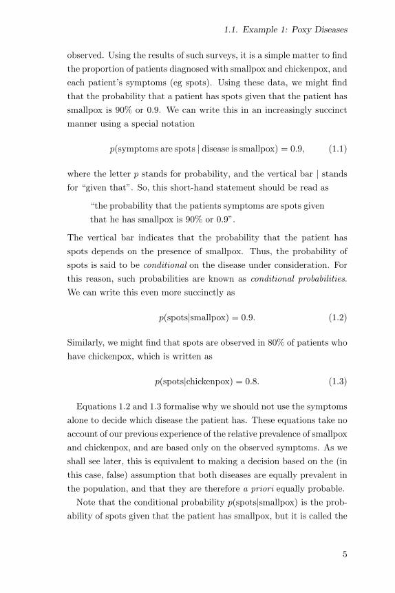
observed. Using the results of such surveys, it is a simple matter to find

the proportion of patients diagnosed with smallpox and chickenpox, and

each patient’s symptoms (eg spots). Using these data, we might find

that the probability that a patient has spots given that the patient has

smallpox is 90% or 0.9. We can write this in an increasingly succinct

manner using a special notation

p(symptoms are spots | disease is smallpox) = 0.9, (1.1)

where the letter p stands for probability, and the vertical bar | standsfor “given that”. So, this short-hand statement should be read as

“the probability that the patients symptoms are spots given

that he has smallpox is 90% or 0.9”.

The vertical bar indicates that the probability that the patient has

spots depends on the presence of smallpox. Thus, the probability of

spots is said to be conditional on the disease under consideration. For

this reason, such probabilities are known as conditional probabilities.

We can write this even more succinctly as

p(spots|smallpox) = 0.9. (1.2)

Similarly, we might find that spots are observed in 80% of patients who

have chickenpox, which is written as

p(spots|chickenpox) = 0.8. (1.3)

Equations 1.2 and 1.3 formalise why we should not use the symptoms

alone to decide which disease the patient has. These equations take no

account of our previous experience of the relative prevalence of smallpox

and chickenpox, and are based only on the observed symptoms. As we

shall see later, this is equivalent to making a decision based on the (in

this case, false) assumption that both diseases are equally prevalent in

the population, and that they are therefore a priori equally probable.

Note that the conditional probability p(spots|smallpox) is the prob-

ability of spots given that the patient has smallpox, but it is called the

5


likelihood of smallpox (which is confusing, but standard, nomenclature).

In this example, the disease smallpox has a larger likelihood than

chickenpox. Indeed, as there are only two diseases under consideration,

this means that, of the two possible alternatives, smallpox has the

maximum likelihood. The disease with the maximum value of likelihood

is known as the maximum likelihood estimate (MLE) of the disease that

the patient has. Thus, in this case, the MLE of the disease is smallpox.

As discussed above, it would be hard to argue that we should disre-

gard our knowledge or previous experience when deciding which disease

the patient has. But exactly how should this previous experience

be combined with current evidence (eg symptoms)? From a purely

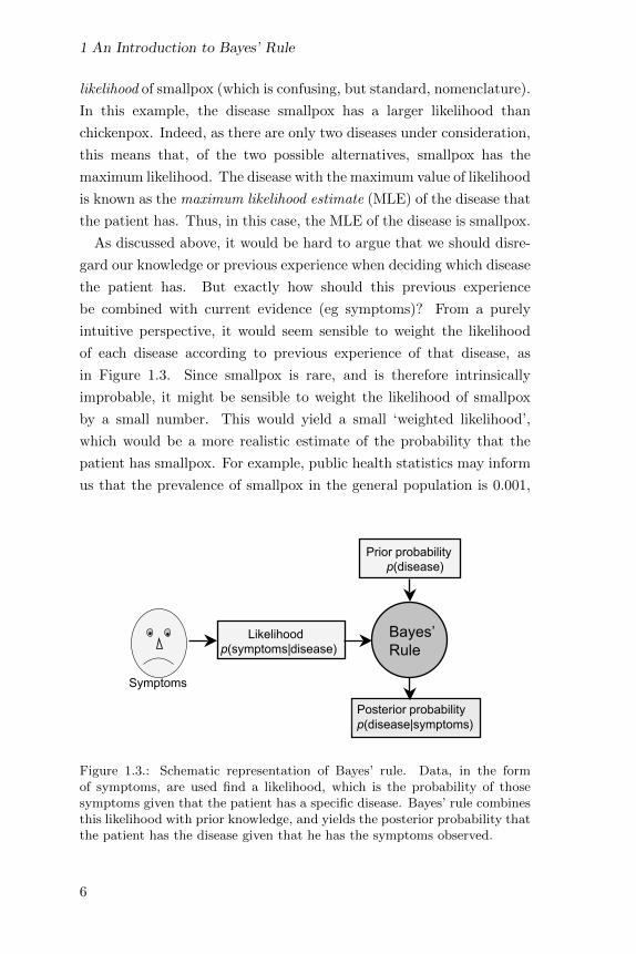
intuitive perspective, it would seem sensible to weight the likelihood

of each disease according to previous experience of that disease, as

in Figure 1.3. Since smallpox is rare, and is therefore intrinsically

improbable, it might be sensible to weight the likelihood of smallpox

by a small number. This would yield a small ‘weighted likelihood’,

which would be a more realistic estimate of the probability that the

patient has smallpox. For example, public health statistics may inform

us that the prevalence of smallpox in the general population is 0.001,

Prior probability

p(disease)

Posterior probability

p(disease|symptoms)

Likelihood

p(symptoms|disease)

Bayes’

Rule

Symptoms

Figure 1.3.: Schematic representation of Bayes’ rule. Data, in the formof symptoms, are used find a likelihood, which is the probability of thosesymptoms given that the patient has a specific disease. Bayes’ rule combinesthis likelihood with prior knowledge, and yields the posterior probability thatthe patient has the disease given that he has the symptoms observed.

6


meaning that there is a one in a thousand chance that a randomly

chosen individual has smallpox. Thus, the probability that a randomly

chosen individual has smallpox is

p(smallpox) = 0.001. (1.4)

This represents our prior knowledge about the disease in the population

before we have observed our patient, and is known as the prior

probability that any given individual has smallpox. As our patient

(before we have observed his symptoms) is as likely as any other

individual to have smallpox, we know that the prior probability that

he has smallpox is 0.001.

If we follow our commonsense prescription, and simply weight (ie

multiply) each likelihood by its prior probability then we obtain ‘weighted

likelihood’ quantities which take account of the current evidence and

of our prior knowledge of each disease. In short, this commonsense

prescription leads to Bayes’ rule. Even so, the equation for Bayes’ rule

given below is not obvious, and should be taken on trust for now. In

the case of smallpox, Bayes’ rule is

p(smallpox|spots) = p(spots|smallpox)⇥ p(smallpox)

p(spots). (1.5)

The term p(spots) in the denominator of Equation 1.5 is the proportion

of people in the general population that have spots, and therefore

represents the probability that a randomly chosen individual has spots.

As will be explained on p15, this term is often disregarded, but we

use a value that makes our sums come out neatly, and assume that

p(spots) = 0.081 (ie 81 in every 1,000 individuals has spots). If we now

substitute numbers into this equation then we obtain

p(smallpox|spots) = 0.9⇥ 0.001/0.081 (1.6)

= 0.011, (1.7)

which is the conditional probability that the patient has smallpox given

that his symptoms are spots.

7


Crucially, the ‘weighted likelihood’ p(smallpox|spots) is also a condi-

tional probability, but it is the probability of the disease smallpox given

the symptoms observed, as shown in Figure 1.4. So, by making use of

prior experience, we have transformed the conditional probability of

the observed symptoms given a specific disease (the likelihood, which

is based only on the available evidence) into a more useful conditional

probability: the probability that the patient has a particular disease

(smallpox) given that he has particular symptoms (spots).

In fact, we have just made use of Bayes’ rule to convert one condi-

tional probability, the likelihood p(spots|smallpox) into a more useful

conditional probability, which we have been calling a ‘weighted likeli-

hood’, but is formally known as the posterior probability p(smallpox|spots).As noted above, both p(smallpox|spots) and p(spots|smallpox) are

conditional probabilities, which have the same status from a mathemat-

ical viewpoint. However, for Bayes’ rule, we treat them very di↵erently.

The conditional probability p(spots|smallpox) is based only on the

observed data (symptoms), and is therefore easier to obtain than

the conditional probability we really want, namely p(smallpox|spots),which is also based on the observed data, but also on prior knowl-

edge. For historical reasons, these two conditional probabilities have

special names. As we have already seen, the conditional probability

p(spots|smallpox) is the probability that a patient has spots given

that he has smallpox, and is known as the likelihood of smallpox.

The complementary conditional probability p(smallpox|spots) is the

posterior probability that a patient has smallpox given that he has

spots. In essence, Bayes’ rule is used to combine prior experience (in

the form of a prior probability) with observed data (spots) (in the

form of a likelihood) to interpret these data (in the form of a posterior

probability). This process is known as Bayesian inference.

The Perfect Inference Engine

Bayesian inference is not guaranteed to provide the correct answer.

Instead, it provides the probability that each of a number of alternative

answers is true, and these can then be used to find the answer that is

most probably true. In other words, it provides an informed guess.

8


p(x|s) = 0.9

Diseasec

Diseases

Frequency in

population

p(s) = 0.0011

Frequency in

population

p(c) = 0.1

p(x|c) = 0.8

= p(x|c)p(

c)/p(x)

= 0.8 x 0.1/0.081

= 0.988

= p(x|s)p(

s)/p(x)

= 0.9 x 0.001/ 0.081

= 0.011

p(c|x) p(

s|x)

Likelihood Likelihood

Prior probability ofc

Prior probability ofs

Posterior probability ofc

Posterior probability ofs

Symptoms x

Bayes’

Rule

Bayes’

Rule

Key

Chickenpox = c

Smallpox = s

Symptoms = x

Figure 1.4.: Comparing the probability of chickenpox and smallpox usingBayesian inference. The observed symptoms x seem to be more consistentwith smallpox ✓

s

than chickenpox ✓s

, as indicated by their likelihood values.However, the background rate of chickenpox in the population is higher thanthat of smallpox, which, in this case, makes it more probable that the patienthas chickenpox, as indicated by its higher posterior probability.

While this may not sound like much, it is far from random guessing.

Indeed, it can be shown that no other procedure can provide a better

guess, so that Bayesian inference can be justifiably interpreted as the

output of a perfect guessing machine, a perfect inference engine (see

Section 4.9, p92). This perfect inference engine is fallible, but it is

provably less fallible than any other.

Making a Diagnosis

In order to make a diagnosis, we need to know the posterior probability

of both of the diseases under consideration. Once we have both

posterior probabilities, we can compare them in order to choose the

disease that is most probable given the observed symptoms.

Suppose that the prevalence of chickenpox in the general population

is 10% or 0.1. This represents our prior knowledge about chickenpox

9


before we have observed any symptoms, and is written as

p(chickenpox) = 0.1, (1.8)

which is the prior probability of chickenpox. As was done in Equation

1.6 for smallpox, we can weight the likelihood of chickenpox with its

prior probability to obtain the posterior probability of chickenpox

p(chickenpox|spots) = p(spots|chickenpox)⇥ p(chickenpox)/p(spots)

= 0.8⇥ 0.1/0.081

= 0.988. (1.9)

The two posterior probabilities, summarised in Figure 1.4, are therefore

p(smallpox|spots) = 0.011 (1.10)

p(chickenpox|spots) = 0.988. (1.11)

Thus, the posterior probability that the patient has smallpox is 0.011,

and the posterior probability that the patient has chickenpox is 0.988.

Aside from a rounding error, these sum to one.

Notice that we cannot be certain that the patient has chickenpox, but

we can be certain that there is a 98.8% probability that he does. This

is not only our best guess, but it is provably the best guess that can be

obtained; it is e↵ectively the output of a perfect inference engine.

In summary, if we ignore all previous knowledge regarding the

prevalence of each disease then we have to use the likelihoods to decide

which disease is present. The likelihoods shown in Equations 1.2 and

1.3 would lead us to diagnose the patient as probably having smallpox.

However, a more informed decision can be obtained by taking account of

prior information regarding the diseases under consideration. When we

do take account of prior knowledge, Equations 1.10 and 1.11 indicate

that the patient probably has chickenpox. In fact, these equations

imply that the patient is about 89 (=0.988/0.011) times more likely

to have chickenpox than smallpox. As we shall see later, this ratio of

10


posterior probabilities plays a key role in Bayesian statistical analysis

(Section 1.1, p14).

Taking account of previous experience yields the diagnosis that is

most probable, given the evidence (spots). As this is the decision

associated with the maximum value of the posterior probability, it is

known as the maximum a posteriori or MAP estimate of the disease.

The equation used to perform Bayesian inference is called Bayes’

rule, and in the context of diagnosis is

p(disease|symptoms) =p(symptoms|disease)p(disease)

p(symptoms), (1.12)

which is easier to remember as

posterior =likelihood⇥ prior

marginal likelihood. (1.13)

The marginal likelihood is also known as evidence, and we shall have

more to say about it shortly.

Bayes’ Rule: Hypothesis and Data

If we consider a putative disease to represent a specific hypothesis, and

the symptoms to be some observed data then Bayes’ rule becomes

p(hypothesis|data) =p(data|hypothesis)⇥ p(hypothesis)

p(data),

where the word “hypothesis” should be interpreted as, “hypothesis is

true”. Written in this form, the contrast between the likelihood and

the posterior probability is more apparent. Specifically, the probability

that the proposed hypothesis is true given some data that were actually

observed is the posterior probability

p(hypothesis|data), (1.14)

11


whereas the probability of observing the data given that the hypothesis

is true is the likelihood

p(data|hypothesis). (1.15)

A More Succinct Notation

We now introduce a succinct, and reasonably conventional, notation for

the terms defined above. There is nothing new in the mathematics of

this section, just a re-writing of equations used above. If we represent

the observed symptoms by x, and the disease by the Greek letter theta

✓s

(where the subscript s stands for smallpox) then we can write the

conditional probability (ie the likelihood of smallpox) in Equation 1.2

p(x|✓s

) = p(spots|smallpox) = 0.9. (1.16)

Similarly, the background rate of smallpox ✓s

in the population can be

represented as the prior probability

p(✓s

) = p(smallpox) = 0.001, (1.17)

and the probability of the symptoms (the marginal likelihood) is

p(x) = p(spots) = 0.081. (1.18)

Substituting this notation into Equation 1.5 (repeated here)

p(smallpox|spots) = p(spots|smallpox)⇥ p(smallpox)

p(spots), (1.19)

yields

p(✓s

|x) =p(x|✓

s

)⇥ p(✓s

)

p(x). (1.20)

12


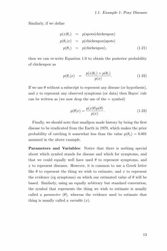
Similarly, if we define

p(x|✓c

) = p(spots|chickenpox)

p(✓c

|x) = p(chickenpox|spots)

p(✓c

) = p(chickenpox), (1.21)

then we can re-write Equation 1.9 to obtain the posterior probability

of chickenpox as

p(✓c

|x) =p(x|✓

c

)⇥ p(✓c

)

p(x). (1.22)

If we use ✓ without a subscript to represent any disease (or hypothesis),

and x to represent any observed symptoms (or data) then Bayes’ rule

can be written as (we now drop the use of the ⇥ symbol)

p(✓|x) = p(x|✓)p(✓)p(x)

. (1.23)

Finally, we should note that smallpox made history by being the first

disease to be eradicated from the Earth in 1979, which makes the prior

probability of catching it somewhat less than the value p(✓s

) = 0.001

assumed in the above example.

Parameters and Variables: Notice that there is nothing special

about which symbol stands for disease and which for symptoms, and

that we could equally well have used ✓ to represent symptoms, and

x to represent diseases. However, it is common to use a Greek letter

like ✓ to represent the thing we wish to estimate, and x to represent

the evidence (eg symptoms) on which our estimated value of ✓ will be

based. Similarly, using an equally arbitrary but standard convention,

the symbol that represents the thing we wish to estimate is usually

called a parameter (✓), whereas the evidence used to estimate that

thing is usually called a variable (x).

13


Model Selection, Posterior Ratios and Bayes Factors

As noted above, when we take account of prior knowledge, it turns out

that the patient is about 90 times more likely (ie 0.988 vs 0.011) to have

chickenpox than smallpox. Indeed, it is often the case that we wish to

compare the relative probabilities of two hypotheses (eg diseases). As

each hypothesis acts as a (simple) model for the data, and we wish to

select the most probable model, this is known as model selection, which

involves a comparison using a ratio of posterior probabilities.

The posterior ratio, which is also known as the posterior odds between

the hypotheses ✓c

and ✓s

, is

Rpost

=p(✓

c

|x)p(✓

s

|x) . (1.24)

If we apply Bayes’ rule to the numerator and denominator then

Rpost

=p(x|✓

c

)p(✓c

)/p(x)

p(x|✓s

)p(✓s

)/p(x), (1.25)

where the marginal likelihood p(x) cancels, so that

Rpost

=p(x|✓

c

)

p(x|✓s

)⇥ p(✓

c

)

p(✓s

). (1.26)

This is a product of two ratios, the ratio of likelihoods, or Bayes factor

B =p(x|✓

c

)

p(x|✓s

), (1.27)

and the ratio of priors, or prior odds between ✓c

and ✓s

, which is

Rprior

= p(✓c

)/p(✓s

). (1.28)

Thus, the posterior odds can be written as

Rpost

= B ⇥Rprior

, (1.29)

14


which, in words, is: posterior odds = Bayes factor ⇥ prior odds. In

this example, we have

Rpost

=0.80

0.90⇥ 0.1

0.001= 88.9.

Note that the likelihood ratio (Bayes factor) is less than one (and so

favours ✓s

), whereas the prior odds is much greater than one (and

favours ✓c

), with the result that the posterior odds come out massively

in favour of ✓c

. If the posterior odds is greater than 3 or less than 1/3

(in both cases one hypothesis is more than 3 times more probable than

the other) then this is considered to represent a substantial di↵erence

between the probabilities of the two hypotheses19, so a posterior odds

of 88.9 is definitely substantial.

Ignoring the Marginal Likelihood

As promised, we consider the marginal likelihood p(symptoms) or p(x)

briefly here (and in Chapter 2 and Section 4.5). The marginal likelihood

refers to the probability that a randomly chosen individual has the

symptoms that were actually observed, which we can interpret as the

prevalence of spots in the general population.

Crucially, the decision as to which disease the patient has depends

only on the relative sizes of di↵erent posterior probabilities (eg Equa-

tions 1.10, 1.11, and in Equations 1.20,1.22). Note that each of these

posterior probabilities is proportional to 1/p(symptoms) in Equations

1.10, 1.11, also expressed as 1/p(x) in Equations 1.20,1.22. This means

that a di↵erent value of the marginal probability p(symptoms) would

change all of the posterior probabilities by the same proportion, and

therefore has no e↵ect on their relative magnitudes. For example, if

we arbitrarily decided to double the value of the marginal likelihood

from 0.081 to 0.162 then both posterior probabilities would be halved

(from 0.011 and 0.988 to about 0.005 and 0.494), but the posterior

probability of chickenpox would still be 88.9 times larger than the

posterior probability of smallpox. Indeed, the previous section on Bayes

factors relies on the fact that the ratio of two posterior probabilities is

independent of the value of the marginal probability.

15


In summary, the value of the marginal probability has no e↵ect on

which disease yields the largest posterior probability (eg Equations 1.10

and 1.11), and therefore has no e↵ect on the decision regarding which

disease the patient probably has.

1.2. Example 2: Forkandles

The example above is based on medical diagnosis, but Bayes’ rule can

be applied to any situation where there is uncertainty regarding the

value of a measured quantity, such as the acoustic signal that reaches

the ear when some words are spoken. The following example follows a

similar line of argument as the previous one, and aside from the change

in context, provides no new information for the reader to absorb.

If you walked into a hardware store and asked, Have you got fork

handles?, then you would be surprised to be presented with four

candles. Even though the phrases fork handles and four candles are

acoustically almost identical, the shop assistant knows that he sells

many more candles than fork handles (Figure 1.5). This in turn, means

that he probably does not even hear the words fork handles, but instead

hears four candles. What has this got to do with Bayes’ rule?

The acoustic data that correspond to the sounds spoken by the cus-

tomer are equally consistent with two interpretations, but the assistant

assigns a higher weighting to one interpretation. This weighting is

based on his prior experience, so he knows that customers are more

likely to request four candles than fork handles. The experience of the

Acoustic data

Four candles?

Fork handles?

?

Figure 1.5.: Thomas Bayes trying to make sense of a London accent, whichremoves the h sound from the word handle, so the phrase fork handles ispronounced fork ’andles, and therefore sounds like four candles (see ForkHandles YouTube clip by The Two Ronnies).

16


assistant allows him to hear what was probably said by the customer,

even though the acoustic data was pretty ambiguous. Without knowing

it, he has probably used something like Bayes’ rule to hear what the

customer probably said.

Likelihood: Answering the Wrong Question

Given that the two possible phrases are four candles and fork handles,

we can formalise this scenario by considering the probability of the

acoustic data given each of the two possible phrases. In both cases, the

probability of the acoustic data depends on the words spoken, and this

dependence is made explicit as two probabilities:

1) the probability of the acoustic data given four candles was spoken,

2) the probability of the acoustic data given fork handles was spoken.

A short-hand way of writing these is

p(acoustic data|four candles)

p(acoustic data|fork handles), (1.30)

where the expression p(acoustic data|four candles), for example, is in-

terpreted as the likelihood that the phrase spoken was four candles.

As both phrases are consistent with the acoustic data, the probability

of the data is almost the same in both cases. That is, the probability

of the data given that four candles was spoken is almost the same as

the probability of the data given that fork handles was spoken. For

simplicity, we will assume that these probabilities are

p(data|four candles) = 0.6

p(data|fork handles) = 0.7. (1.31)

Knowing these two likelihoods does allow us to find an answer, but it

is an answer to the wrong question. Each likelihood above provides an

answer to the (wrong) question: what is the probability of the observed

acoustic data given that each of two possible phrases was spoken?

17


Posterior Probability: Answering the Right Question

The right question, the question to which we would like an answer is:

what is the probability that each of the two possible phrases was spoken

given the acoustic data? The answer to this, the right question, is

implicit in two new conditional probabilities, the posterior probabilities

p(four candles|data)

p(fork handles|data), (1.32)

as shown in Figures 1.6 and 1.7. Notice the subtle di↵erence between

the pair of Equations 1.31 and the pair 1.32. Equations 1.31 tells us

the likelihoods, the probability of the data given two possible phrases,

which turn out to be almost identical for both phrases in this example.

In contrast, Equations 1.32 tells us the posterior probabilities, the

probability of each phrase given the acoustic data.

Crucially, each likelihood tells us the probability of the data given

a particular phrase, but takes no account of how often that phrase

has been given (ie has been encountered) in the past. In contrast,

each posterior probability depends, not only on the data (in the form

of the likelihood), but also on how frequently each phrase has been

encountered in the past; that is, on prior experience.

So, we want the posterior probability, but we have the likelihood.

Fortunately, Bayes’ rule provides a means of getting from the likelihood

to the posterior, by making use of extra knowledge in the form of prior

experience, as shown in Figure 1.6.

Prior Probability

Let’s suppose that the assistant has been asked for four candles a total

of 90 times in the past, whereas he has been asked for fork handles

only 10 times. To keep matters simple, let’s also assume that the next

customer will ask either for four candles or fork handles (we will revisit

this simplification later). Thus, before the customer has uttered a single

word, the assistant estimates that the probability that he will say each

18


of the two phrases is

p(four candles) = 90/100 = 0.9

p(fork handles) = 10/100 = 0.1. (1.33)

These two prior probabilities represent the prior knowledge of the

assistant, based on his previous experience of what customers say.

When confronted with an acoustic signal that has one of two possible

interpretations, the assistant naturally interprets this as four candles,

because, according to his past experience, this is what such ambiguous

acoustic data usually means in practice. So, he takes the two almost

equal likelihood values, and assigns a weighting to each one, a weighting

that depends on past experience, as in Figure 1.7. In other words, he

uses the acoustic data, and combines it with his previous experience to

make an inference about which phrase was spoken.

Inference

One way to implement this weighting (ie to do this inference) is to

simply multiply the likelihood of each phrase by how often that phrase

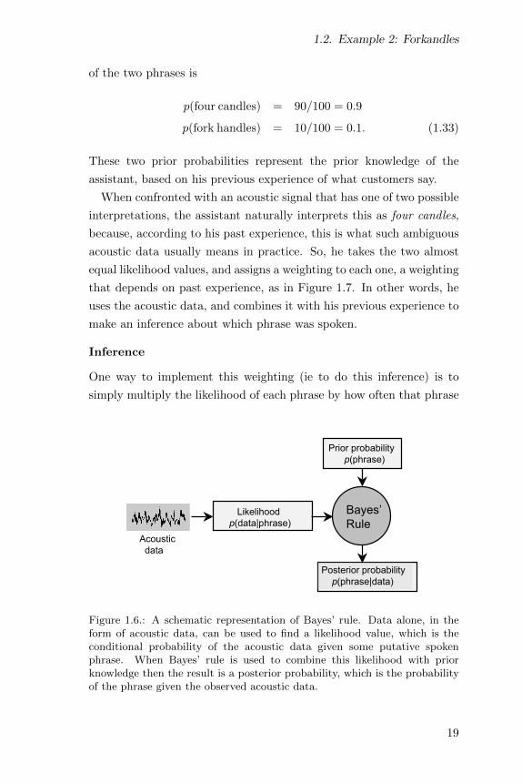
Prior probability

p(phrase)

Posterior probability

p(phrase|data)

Likelihood

p(data|phrase)

Bayes’

Rule

Acoustic

data

Figure 1.6.: A schematic representation of Bayes’ rule. Data alone, in theform of acoustic data, can be used to find a likelihood value, which is theconditional probability of the acoustic data given some putative spokenphrase. When Bayes’ rule is used to combine this likelihood with priorknowledge then the result is a posterior probability, which is the probabilityof the phrase given the observed acoustic data.

19


p(x|h) = 0.7

Phrasec

Phraseh

Frequency

p(h) = 0.1

Frequency

p(c) = 0.9

p(x|c) = 0.6

= p(x|c)p(

c)/p(x)

= 0.6 x 0.9/0.61

= 0.885

= p(x|h)p(

h)/p(x)

= 0.7 x 0.1/0.61

= 0.115

p(c|x) p(

h|x)

Likelihood of c Likelihood of

h

Prior probability of c

Prior probability of h

Posterior probability of c

Posterior probability of h

Acoustic signal x

Bayes’

Rule

Bayes’

Rule

Figure 1.7.: Bayesian inference applied to speech data.

has occurred in the past. In other words, we multiply the likelihood of

each putative phrase by its corresponding prior probability. The result

yields a posterior probability for each possible phrase

p(four candles|data) = p(data|four candles)p(four candles)p(data)

p(fork handles|data) = p(data|fork handles)p(fork handles)p(data)

, (1.34)

where p(data) is the marginal likelihood, which is the probability of the

observed data.

In order to ensure that the posterior probabilities sum to one, the

value of p(data) is 0.61 in this example, but as we already know

from Section 1.1 (p15), its value is not important for our purposes.

If we substitute the likelihood and prior probability values defined

in Equations 1.31 and 1.33 in 1.34 then we obtain their posterior

20

1.3. Example 3: Flipping Coins

probabilities as

p(four candles|data) = p(data|four candles)p(four candles)/p(data)

= 0.6⇥ 0.9/0.61 = 0.885,

p(fork handles|data) = p(data|fork handles)p(fork handles)/p(data)

= 0.7⇥ 0.1/0.61 = 0.115.

As in the previous example, we can write this more succinctly by

defining

x = acoustic data,

✓c

= four candles,

✓h

= fork handles,

so that

p(✓c

|x) = p(x|✓c

)p(✓c

)/p(x) = 0.885

p(✓h

|x) = p(x|✓h

)p(✓h

)/p(x) = 0.115. (1.35)

These two posterior probabilities represent the answer to the right

question, so we can now see that the probability that the customer said

four candles is 0.885 whereas the probability that the customer said fork

handles was 0.115. As four candles is associated with the highest value

of the posterior probability, it is the maximum a posteriori (MAP)

estimate of the phrase that was spoken. The process that makes use of

evidence (symptoms) to produce these posterior probabilities is called

Bayesian inference.


This example follows the same line of reasoning as those above, but

also contains specific information on how to combine probabilities from

independent events, such as coin flips. This will prove crucial in a

variety of contexts, and in examples considered later in this book.

21


Here, our task is to decide how unfair a coin is, based on just two

coin flips. Normally, we assume that coins are fair or unbiased, so that

a large number of coin flips (eg 1000) yields an equal number of heads

and tails. But suppose there was a fault in the machine that minted

coins, so that each coin had more metal on one side or the other, with

the result that each coin is biased to produce more heads than tails, or

vice versa. Specifically, 25% of the coins produced by the machine have

a bias of 0.4, and 75% have a bias of 0.6. By definition, a coin with a

bias of 0.4 produces a head on 40% of flips, whereas a coin with a bias

of 0.6 produces a head on 60% of flips (on average). Now, suppose we

choose one coin at random, and attempt to decide which of the two bias

values it has. For brevity, we define the coin’s bias with the parameter

✓, so the true value of ✓ for each coin is either ✓0.4 = 0.4, or ✓0.6 = 0.6.

One Coin Flip: Here we use one coin flip to define a few terms that

will prove useful below. For each coin flip, there are two possible

outcomes, a head xh

, and a tail xt

. For example, if the coin’s bias

is ✓0.6 then, by definition, the conditional probability of observing a

head is ✓0.6

p(xh

|✓0.6) = ✓0.6 = 0.6. (1.36)

Similarly, the conditional probability of observing a tail is

p(xt

|✓0.6) = (1� ✓0.6) = 0.4, (1.37)

where both of these conditional probabilities are likelihoods. Note

that we follow the convention of the previous examples by using ✓

Bias=0.6?

Bias=0.4?

?..

Figure 1.8.: Thomas Bayes trying to decide the value of a coin’s bias.

22


to represent the parameter whose value we wish to estimate, and x to

represent the data used to estimate the true value of ✓.

Two Coin Flips: Consider a coin with a bias ✓ (where ✓ could be 0.4

or 0.6, for example). Suppose we flip this coin twice, and obtain a head

xh

followed by a tail xt

, which define the ordered list or permutation

x = (xh

, xt

). (1.38)

As the outcome of one flip is not a↵ected by any other flip outcome,

outcomes are said to be independent (see Section 2.2 or Appendix C).

This independence means that the probability of observing any two

outcomes can be obtained by multiplying their probabilities

p(x|✓) = p((xh

, xt

)|✓) (1.39)

= p(xh

|✓)⇥ p(xt

|✓). (1.40)

More generally, for a coin with a bias ✓, the probability of a head xh

is

p(xh

|✓) = ✓, and the probability of a tail xt

is therefore p(xt

|✓) = (1�✓).

It follows that Equation 1.40 can be written as

p(x|✓) = ✓ ⇥ (1� ✓), (1.41)

which will prove useful below.

Data xPrior probability p(!)

Posterior probability p(!|x)

Likelihood p(x|!)

Bayes’

Rule

Figure 1.9.: A schematic representation of Bayes’ rule, applied to the problemof estimating the bias of a coin based on data which is the outcome of twocoin flips.

23


The Likelihoods of Di↵erent Coin Biases: According to Equation

1.41, if the coin bias is ✓0.6 then

p(x|✓0.6) = ✓0.6 ⇥ (1� ✓0.6) (1.42)

= 0.6⇥ 0.4 (1.43)

= 0.24, (1.44)

and if the coin bias is ✓0.4 then (the result is the same)

p(x|✓0.4) = ✓0.4 ⇥ (1� ✓0.4) (1.45)

= 0.4⇥ 0.6 (1.46)

= 0.24. (1.47)

Note that the only di↵erence between these two cases is the reversed

ordering of terms in Equations 1.43 and 1.46, so that both values of ✓

have equal likelihood values. In other words, the observed data x are

equally probable given the assumption that ✓0.4 = 0.4 or ✓0.6 = 0.6, so

they do not help in deciding which bias our chosen coin has.

p(x|!0.6

) = 0.24

Bias !0.4

Bias !0.6

Frequency

p(!0.6

) = 0.75

Frequency

p(!0.4

) = 0.25

p(x|!0.4

) = 0.24

= p(x|!0.4

) p(!0.4

)/p(x)

= 0.24 x 0.25/0.24

= 0.25

= p(x|!0.6

) p(!0.6

)/p(x)

= 0.24 x 0.75/0.24

= 0.75

p(!0.4

|x) p(!0.6

|x)

Likelihood of !0.4

Likelihood of !0.6

Prior probability of !0.4

Prior probability of !0.6

Posterior probability of !0.4

Posterior probability of !0.6

Data x = 2 coin flip outcomes

Bayes’

Rule

Bayes’

Rule

Figure 1.10.: Bayesian inference applied to coin flip data.

24

1.4. Example 4: Light Craters

Prior Probabilities of Di↵erent Coin Biases: We know (from

above) that 25% of all coins have a bias of ✓0.4, and that 75% of all

coins have a bias of ✓0.6. Thus, even before we have chosen our coin,

we know (for example) there is a 75% chance that it has a bias of 0.6.

This information defines the prior probability that any coin has one of

two bias values, either p(✓0.4) = 0.25, or p(✓0.6) = 0.75.

Posterior Probabilities of Di↵erent Coin Biases: As in previous

examples, we adopt the naıve strategy of simply weighting each likeli-

hood value by its corresponding prior (and dividing by p(x)) to obtain

Bayes’ rule

p(✓0.4|x) = p(x|✓0.4)p(✓0.4)/p(x)

= 0.24⇥ 0.25/0.24

= 0.25, (1.48)

p(✓0.6|x) = p(x|✓0.6)p(✓0.6)/p(x)

= 0.24⇥ 0.75/0.24

= 0.75. (1.49)

In order to ensure posterior probabilities sum to one, we have assumed

a value for the marginal probability of p(x) = 0.24 (but we know from

p15 that its value makes no di↵erence to our final decision about coin

bias). As shown in Figures 1.9 and 1.10, the probabilities in Equations

1.48 and 1.49 take account of both the data and of prior experience,

and are therefore posterior probabilities. In summary, whereas the

equal likelihoods in this example (Equations 1.44 and 1.47) did not

allow us to choose between the coin biases ✓0.4 and ✓0.6, the values of

the posterior probabilities (Equations 1.48 and 1.49) imply that a bias

of ✓0.6 is 3 (=0.75/0.25) times more probable than a bias is ✓0.4.

1.4. Example 4: Light Craters

When you look at Figure 1.11, do you see a hill or a crater? Now turn

the page upside-down. When you invert the page, the content of the

picture does not change, but what you see does change (from a hill

25


Figure 1.11.: Is this a hill or a crater? Try turning the book upside-down.(Barringer crater, with permission, United States Geological Survey).

to a crater). This illusion almost certainly depends on the fact that

your visual system assumes that the scene is lit from above. This, in

turn, forces you to interpret the Figure 1.11 as a hill, and the inverted

version as a crater (which it is, in reality).

In terms of Bayes’ rule, the image data are equally consistent with a

hill and a crater, where each interpretation corresponds to a di↵erent

maximum likelihood value. Therefore, in the absence of any prior

assumptions on your part, you should see the image as depicting either

a hill or a crater with equal probability. However, the assumption

that light comes from above corresponds to a prior, and this e↵ectively

forces you to interpret the image as a hill or a crater, depending on

whether the image is inverted or not. Note that there is no uncertainty

or noise; the image is perfectly clear, but also perfectly ambiguous

without the addition of a prior regarding the light source. This example

demonstrates that Bayesian inference is useful even when there is no

noise in the observed data, and that even the apparently simple act of

seeing requires the use of prior information10;40;41;42:

Seeing is not a direct apprehension of reality, as we often

like to pretend. Quite the contrary: seeing is inference from

incomplete information ...

ET Jaynes, 2003 (p133)18.

26

1.5. Forward and Inverse Probability

1.5. Forward and Inverse Probability

If we are given a coin with a known bias of say, ✓ = 0.6, then the

probability of a head for each coin flip is given by the likelihood

p(xh

|✓) = 0.6. This is an example of a forward probability, which

involves calculating the probability of each of a number of di↵erent

consequences (eg obtaining two heads) given some known cause or fact,

see Figure 1.12. If this coin is flipped a 100 times then the number of

heads could be 62, so the actual proportion of heads is xtrue

= 0.62.

But, because no measurement is perfectly reliable, we may mis-count

62 as 64 heads, so the measured proportion is x = 0.64. So there

is a di↵erence, often called noise, between the true coin bias and the

measured proportion of heads. The source of this noise may be due to

the probabilistic nature of coin flips or to our inability to measure the

number of heads accurately. Whatever the cause of the noise, the only

Physics xtrue Measure x

Modelp(x|!)Bayes’

Rule!est

Prior p(!)

Likelihood

!true

Figure 1.12.: Forward and inverse probability.Top: Forward probability. A parameter value ✓

true

(eg coin bias) whichis implicit in a physical process (eg coin flipping) yields a quantity x

true

(eg proportion of heads), which is measured as x, using an imperfectmeasurement process.Bottom: Inverse probability. Given a mathematical model of the physics thatgenerated x

true

, the measured value x implies a range of possible values forthe parameter ✓. The probability of x given each possible value of ✓ definesa likelihood. When combined with a prior, each likelihood yields a posteriorprobability p(✓|x), which allows an estimate ✓

est

of ✓true

to be obtained.

27


information we have is the measured number of heads, and we must

use this information as wisely as possible.

The converse of reasoning forwards from a given physical parameter

or scenario involves a harder problem, also illustrated in Figure 1.12.

Reasoning backwards from measurements (eg coin flips or images)

amounts to finding the posterior or inverse probability of the value

of an unobserved variable (eg coin bias, 3D shape), which is usually

the cause of the observed measurement. By analogy, arriving at the

scene of a crime, a detective must reason backwards from the clues, as

eloquently expressed by Sherlock Holmes:

Most people, if you describe a train of events to them, will

tell you what the result would be. They can put those

events together in their minds, and argue from them that

something will come to pass. There are few people, however,

who, if you told them a result, would be able to evolve from

their own inner consciousness what the steps were that led

to that result. This power is what I mean when I talk of

reasoning backward, or analytically.

Sherlock Holmes, from A Study in Scarlet. AC Doyle, 1887.

Indeed, finding inverse probabilities is precisely the problem Bayes’ rule

is designed to tackle.

Summary

All decisions should be based on evidence, but the best decisions should

also be based on previous experience. The above examples demonstrate

not only that prior experience is crucial for interpreting evidence, but

also that Bayes’ rule provides a rigorous method for doing so.

28

Chapter 2

Bayes’ Rule in Pictures

Probability theory is nothing but common sense reduced to

calculation.

Pierre-Simon Laplace (1749-1827).

Introduction

Some people understand mathematics through the use of symbols,

but additional insights are often obtained if those symbols can be

translated into geometric diagrams and pictures. In this chapter, once

we have introduced random variables and the basic rules of probability,

several di↵erent pictorial representations of probability will be used to

encourage an intuitive understanding of the logic that underpins those

rules. Having established a firm understanding of these rules, Bayes’

rule follows using a few lines of algebra.

2.1. Random Variables

As in the previous chapter, we define the bias of a coin as its propensity

to land heads up. But now we are familiar with the idea of quantities

(such as coin flip outcomes) that are subject to variability, we can

consider the concept of a random variable. The term random variable

continues in use for historical reasons, although random variables are

not the same as the variables used in algebra, like the x in 3x+ 2 = 5,

where the variable x has a definite, but unknown, value that we can

solve for.

29

Further Reading

Bernardo JM and Smith A (2000)4. Bayesian Theory. A rigorous

account of Bayesian methods, with many real-world examples.

Bishop C (2006)5. Pattern Recognition and Machine Learning. As the

title suggests, this is mainly about machine learning, but it provides a

lucid and comprehensive account of Bayesian methods.

Cowan G (1998)6. Statistical Data Analysis. An excellent non-

Bayesian introduction to statistical analysis.

Dienes Z (2008)8. Understanding Psychology as a Science: An In-

troduction to Scientific and Statistical Inference. Provides tutorial

material on Bayes’ rule and a lucid analysis of the distinction between

Bayesian and frequentist statistics.

Gelman A, Carlin J, Stern H and Rubin D (2003)14. Bayesian Data

Analysis. A rigorous and comprehensive account of Bayesian analysis,

with many real-world examples.

Jaynes E and Bretthorst G (2003)18. Probability Theory: The Logic of

Science. The modern classic of Bayesian analysis. It is comprehensive

and wise. Its discursive style makes it long (600 pages) but never dull,

and it is packed full of insights.

Khan S (2012). Introduction to Bayes’ Theorem.

http://www.khanacademy.org/math/probability/v/probability--part-8

Salman Khan’s online mathematics videos make a good introduction to

various topics, including Bayes’ rule.

149

Further Reading

Lee PM (2004)27. Bayesian Statistics: An Introduction. A rigorous

and comprehensive text with a strident Bayesian style.

MacKay DJC (2003)28. Information theory, inference, and learning

algorithms. The modern classic on information theory. A very readable

text that roams far and wide over many topics, almost all of which make

use of Bayes’ rule.

Migon HS and Gamerman D (1999)30. Statistical Inference: An

Integrated Approach. A straightforward (and clearly laid out) account

of inference, which compares Bayesian and non-Bayesian approaches.

Despite being fairly advanced, the writing style is tutorial in nature.

Pierce JR (1980)34, 2nd Edition. An introduction to information the-

ory: symbols, signals and noise. Pierce writes with an informal, tutorial

style of writing, but does not flinch from presenting the fundamental

theorems of information theory.

Reza FM (1961)35. An introduction to information theory. A more

comprehensive and mathematically rigorous book than the Pierce book

above, and should ideally be read only after first reading Pierce’s more

informal text.

Sivia DS and Skilling J (2006)38. Data Analysis: A Bayesian Tutorial.

This is an excellent tutorial style introduction to Bayesian methods.

Spiegelhalter D and Rice K (2009)36. Bayesian statistics. Scholarpedia,

4(8):5230.

http://www.scholarpedia.org/article/Bayesian_statistics

A reliable and comprehensive summary of the current status of Bayesian

statistics.

150

Appendix A

Glossary

Bayes’ rule Given some observed data x, the posterior probability that

the parameter ⇥ has the value ✓ is p(✓|x) = p(x|✓)p(✓)/p(x),where p(x|✓) is the likelihood, p(✓) is the prior probability of the

value ✓, and p(x) is the marginal probability of the value x.

conditional probability The probability that the value of one random

variable ⇥ has the value ✓ given that the value of another random

variable X has the value x; written as p(⇥ = ✓|X = x) or p(✓|x).

forward probability Reasoning forwards from the known value of a

parameter to the probability of some event defines the forward

probability of that event. For example, if a coin has a bias of ✓

then the forward probability p(xh

|✓) of observing a head xh

is ✓.

independence If two variablesX and ⇥ are independent then the value

x of X provides no information regarding the value ✓ of the other

variable ⇥, and vice versa.

inverse probability Reasoning backwards from an observed measure-

ment xh

(eg coin flip) involves finding the posterior or inverse

probability p(✓|xh

) of an unobserved parameter ✓ (eg coin bias).

joint probability The probability that two or more quantities simulta-

neously adopt specified values. For example, the probability that

a coin flip yields a head xh

and that a (possibly di↵erent) coin

has a bias ✓ is the joint probability p(xh

, ✓).

153

Glossary

likelihood The conditional probability p(x|✓) that the observed data

X has the value x given a putative parameter value ✓ is the

likelihood of ✓, and is often written as L(✓|x). When considered

over all values ⇥ of ✓, p(x|⇥) defines a likelihood function.

marginal distribution The distribution that results from marginalisa-

tion of a multivariate (eg 2D) distribution. For example, the

2D distribution p(X,⇥) shown in Figure 3.4 has two marginal

distributions, which, in this case, are the prior distribution p(⇥)

and the distribution of marginal likelihoods p(X).

maximum a posteriori (MAP) Given some observed data x, the value

✓MAP

of an unknown parameter ⇥ that makes the posterior prob-

ability p(⇥|x) as large as possible is the maximum a posteriori

or MAP estimate of the true value ✓true

of that parameter. The

MAP takes into account both the current evidence in the form of

x as well as previous knowledge in the form of prior probabilities

p(⇥) regarding each value of ✓.

maximum likelihood estimate (MLE) Given some observed data x,

the value ✓MLE

of an unknown parameter ⇥ that makes the

likelihood function p(x|⇥) as large as possible is the maximum

likelihood estimate (MLE) of the true value of that parameter.

noise Usually considered to be the random jitter that is part of a

measured quantity.

non-informative prior See reference prior, and Section 4.8.

parameter A variable (often a random variable), which is part of an

equation which, in turn, acts as a model for observed data.

posterior The posterior probability p(✓|x) is the probability that a

parameter ⇥ has the value ✓, based on current evidence (data,

x) and prior knowledge. When considered over all values of ✓, it

refers to the posterior probability distribution p(⇥|x).

154

Glossary

prior The prior probability p(✓) is the probability that the random

variable ⇥ adopts the value ✓. When considered over all values

⇥, it is the prior probability distribution p(⇥).

probability There are many definitions of probability. The two main

ones are (using coin bias as an example): 1) Bayesian proba-

bility: an observer’s estimate of the probability that a coin will

land heads up is based on all the information the observer has,

including the proportion of times it was observed to land heads

up in the past. 2) Frequentist probability: the probability that

a coin will land heads up is given by the proportion of times it

lands heads up, when measured over a large number of coin flips.

probability density function (pdf) The function p(⇥) of a continuous

random variable ⇥ defines the probability density of each possible

value of ⇥. The probability that ⇥ = ✓ can be considered as the

probability density p(✓) (it is actually the product p(✓)⇥ d✓).

probability distribution The distribution of probabilities of di↵erent

values of a variable. The probability distribution of a continuous

variable is a probability density function, and the probability

distribution of a discrete variable is a probability function. When

we refer to a case which includes either continuous or discrete

variables, we use the term probability distribution in this text.

probability function (pf) A function p(⇥) of a discrete random vari-

able ⇥ defines the probability of each possible value of ⇥. The

probability that ⇥ = ✓ is p(⇥ = ✓) or more succinctly p(✓). This

is called a probability mass function (pmf) in some texts.

product rule The joint probability p(x, ✓) is given by the product of

the conditional probability p(x|✓) and the probability p(✓); that

is, p(x, ✓) = p(x|✓)p(✓). See Appendix C.

random variable (RV) Each value of a random variable can be consid-

ered as one possible outcome of an experiment that has a number

of di↵erent possible outcomes, such as the throw of a die. The set

155

Glossary

of possible outcomes is the sample space of a random variable. A

discrete random variable has a probability function (pf), which

assigns a probability to each possible value. A continuous random

variable has a probability density function (pdf), which assigns a

probability density to each possible value. Upper case letters (eg

X) refer to random variables, and (depending on context) to the

set of all possible values of that variable. See Section 2.1, p29.

real number A number that can have any value corresponding to the

length of a continuous line.

regression A technique used to fit a parametric curve (eg a straight

line) to a set of data points.

reference prior A prior distribution that is ‘fair’. See Section 4.8, p91

and Appendix H, p177.

standard deviation The standard deviation of a variable is a measure

of how ‘spread out’ its values are. If we have a sample of n values

of a variable x then the standard deviation of our sample is

� =

vuut 1

n

nX

i=1

(xi

� x)2, (A.1)

where x is the mean of our sample. The sample’s variance is �2.

sum rule This states that the probability p(x) that X = x is the sum

of joint probabilities p(x,⇥), where this sum is taken over all N

possible values of ⇥,

p(x) =NX

i=1

p(x, ✓i

).

Also known as the law of total probability. See Appendix C.

variable A variable is essentially a ‘container’, usually for one number.

We use the lower case (eg x) to refer to a particular value of a

variable.

156

References

[1] Bayes, T. (1763). An essay towards solving a problem in thedoctrine of chances. Phil Trans Roy Soc London, 53:370–418.

[2] Beaumont, M. (2004). The Bayesian revolution in genetics. NatureReviews Genetics, pages 251–261.

[3] Bernardo, J. (1979). Reference posterior distributions for Bayesianinference. J. Royal Statistical Society B, 41:113–147.

[4] Bernardo, J. and Smith, A. (2000). Bayesian Theory. John Wileyand Sons Ltd.

[5] Bishop, C. (2006). Pattern Recognition and Machine Learning.Springer.

[6] Cowan, G. (1998). Statistical Data Analysis. OUP.

[7] Cox, R. (1946). Probability, frequency, and reasonable expectation.American Journal of Physics, 14:113.

[8] Dienes, Z. (2008). Understanding Psychology as a Science:An Introduction to Scientific and Statistical Inference. PalgraveMacmillan.

[9] Donnelly, P. (2005). Appealing statistics. Significance, 2(1):46–48.

[10] Doya, K., Ishii, S., Pouget, A., and Rao, R. (2007). The BayesianBrain. MIT, MA.

[11] Efron, B. (1979). Bootstrap methods: Another look at thejackknife. Ann. Statist., 7(1):1–26.

[12] Frank, M. C. and Goodman, N. D. (2012). Predicting pragmaticreasoning in language games. Science, 336(6084):998.

[13] Geisler, W. and Diehl, R. (2002). Bayesian natural selection andthe evolution of perceptual systems. Philosophical Transactions ofthe Royal Society London (B) Biology, 357:419–448.

185

References

[14] Gelman, A., Carlin, J., Stern, H., and Rubin, D. (2003). BayesianData Analysis, Second Edition. Chapman and Hall, 2nd edition.

[15] Geman, S. and Geman, D. (1993). Stochastic relaxation, Gibbsdistributions and the Bayesian restoration of images. Journal ofApplied Statistics, 20:25–62.

[16] Good, I. (1979). Studies in the history of probability and statistics.XXXVII A. M. Turing’s statistical work inWorldWar II. Biometrika,66(2):393–396.

[17] Hobson, M., Ja↵e, A., Liddle, A., and Mukherjee, P. (2009).Bayesian Methods in Cosmology. Cambridge University Press.

[18] Jaynes, E. and Bretthorst, G. (2003). Probability Theory: TheLogic of Science. Cambridge University Press, Cambridge.

[19] Je↵reys, H. (1939). Theory of Probability. Oxford University Press.

[20] Jones, M. and Love, B. (2011). Bayesian fundamentalism orenlightenment? status and theoretical contributions of Bayesianmodels of cognition. Behavioral and Brain Sciences, 34:192–193.

[21] Kadane, J. (2009). Bayesian thought in early modern detectivestories: Monsieur Lecoq, C. Auguste Dupin and Sherlock Holmes.Statistical Science, 24(2):238–243.

[22] Kersten, D., Mamassian, P., and Yuille, A. (2004). Objectperception as Bayesian inference. Ann Rev Psychology, 55(1):271–304.

[23] Knill, D. and Richards, R. (1996). Perception as Bayesianinference. Cambridge University Press, New York, NY, USA.

[24] Kolmogorov, A. (1933). Foundations of the Theory of Probability.Chelsea Publishing Company, (English translation, 1956).

[25] Land, M. and Nilsson, D. (2002). Animal eyes. OUP.

[26] Lawson, A. (2008). Bayesian Disease Mapping: HierarchicalModeling in Spatial Epidemiology. Chapman and Hall.

[27] Lee, P. (2004). Bayesian Statistics: An Introduction. Wiley.

[28] MacKay, D. (2003). Information theory, inference, and learningalgorithms. Cambridge University Press.

[29] McGrayne, S. (2011). The Theory That Would Not Die. YUP.

186

References

[30] Migon, H. and Gamerman, D. (1999). Statistical Inference: AnIntegrated Approach. Arnold.

[31] Oaksford, M. and Chater, N. (2007). Bayesian Rationality: Theprobabilistic approach to human reasoning. Oxford University Press.

[32] Parent, E. and Rivot, E. (2012). Bayesian Modeling of EcologicalData. Chapman and Hall.

[33] Penny, W. D., Trujillo-Barreto, N. J., and Friston, K. J. (2005).Bayesian fMRI time series analysis with spatial priors. NeuroImage,24(2):350–362.

[34] Pierce, J. (1961 reprinted by Dover 1980). An introduction toinformation theory: symbols, signals and noise. Dover (2nd Edition).

[35] Reza, F. (1961). Information Theory. New York, McGraw-Hill.

[36] Rice, D. and Spiegelhalter, K. (2009). Bayesian statistics.Scholarpedia, 4(3):5230.

[37] Simpson, E. (2010). Edward simpson: Bayes at Bletchley park.Significance, 7(2).

[38] Sivia, D. and Skilling, J. (2006). Data Analysis: A BayesianTutorial. OUP.

[39] Stigler, S. (1983). Who discovered Bayes’s theorem? TheAmerican Statistician, 37(4):290–296.

[40] Stone, J. (2011). Footprints sticking out of the sand (PartII): Children’s Bayesian priors for lighting direction and convexity.Perception, 40(2):175–190.

[41] Stone, J. (2012). Vision and Brain: How we perceive the world.MIT Press.

[42] Stone, J., Kerrigan, I., and Porrill, J. (2009). Where is the light?Bayesian perceptual priors for lighting direction. Proceedings RoyalSociety London (B), 276:1797–1804.

[43] Taroni, F., Aitken, C., Garbolino, P., and Biedermann, A. (2006).Bayesian Networks and Probabilistic Inference in Forensic Science.Wiley.

[44] Tenenbaum, J. B., Kemp, C., Gri�ths, T. L., and Goodman, N. D.(2011). How to grow a mind: Statistics, structure, and abstraction.Science, 331(6022):1279–1285.

187

Index

Bayesfactor, 14objective, 91

Bayes’ rule, i, 1, 8, 11, 25, 40,65, 67, 79, 133, 141,144

continuous variables, 73derivation, 40, 43, 65, 144joint distribution, 69medical test, 43Venn diagram, 41

Bayes’ theorem, 2binomial, 74

coe�cient, 149, 151distribution, 87, 149equation, 149

bootstrap, 92

central limit theorem, 103, 104,110

combination, 90, 149, 151conditional probability, 5, 143

definition, 133continuous variable, 48Cox, 3, 31, 126

discrete variable, 48distribution

Gaussian, 95, 96, 102, 107,153

normal, 95binomial, 87

evidence, 11

false alarm rate, 44forward probability, 27, 40, 133frequentist, 119

Gaussian distribution, 95, 96,102, 107, 153

Gull, 128

histogram, 145, 146hit rate, 44

independence, 23, 32, 116definition, 133

inference, 8inverse probability, 27, 38, 133

Jaynes, 31, 91Je↵reys, 31, 73joint probability, 32, 33, 105,

109, 133

Kolmogorov, 3, 31, 126

Laplace, 1, 91, 128least-squares estimate, 99likelihood, 6, 9

definition, 134function, 58, 60, 67, 69, 79,

137unequal, 6

log posteriordistribution, 101probability, 85

loss function, 92

189

Index

MAP, 11, 21, 69, 70marginal

definition, 134likelihood, 14, 15, 54, 56,

67, 68probability, 35probability distribution, 56,

58, 67, 68marginal likelihood, 11marginal probability, 35marginalisation, 56maximum a posteriori, 11, 21,

58, 69, 70, 134maximum likelihood estimate,

6, 69definition, 134

miss rate, 44model selection, 14, 41

noise, 27, 73, 134non-informative prior, 91, 134

objective Bayes, 91odds

posterior, 14, 41prior, 14

parameter, 13, 134permutation, 23, 74, 151posterior

distribution, 58, 67, 69, 137odds, 14, 41probability, 9probability definition, 134probability density function,

79principle

indi↵erence, 91insu�cient reason, 91maximum entropy, 91

priordefinition, 134distribution, 58, 67, 69, 137

non-informative, 91odds, 14probability, 7reference, 82, 91

probabilityBayesian, 119conditional, 143definition, 135density, 146density function, 73, 78, 145density function,definition,

135distribution, 30distribution,definition, 135forward, 27, 40, 133frequentist, 119function, 48function,definition, 135inverse, 27, 38, 133joint, 33, 34, 105, 109, 133rules of, 31, 141subjective, 124

product rule, 31, 33, 38, 135,141, 144

random variable, 29, 73, 135,137

reference prior, 91, 136, 157regression, 104, 136rule

Bayes’, 141product, 33, 38, 141sum, 33, 36, 141

sample space, 30Saunderson, 1, 128scaling factor, 85set, 30Sherlock Holmes, 1, 2, 28, 47,

109sum rule, 33, 36, 56, 136, 141,

144

Turing, 2

190

About the Author.Dr James Stone is a Reader in Vision and Computational Neuroscienceat the University of She�eld, England.

Information Theory: A Tutorial Introduction,JV Stone, 2014 (forthcoming).

Vision and Brain: How We Perceive the World, JV Stone,MIT Press, 2012.

Seeing: The Computational Approach to Biological Vision,JP Frisby and JV Stone, MIT Press, 2010.

Independent Component Analysis: A Tutorial Introduction,JV Stone, MIT Press, 2004.

SeeingThe Computational Approach to Biological Vision

John P. Frisby and James V. Stone

second edition

Bayes’ Rule: A Tutorial Introduction to Bayesian AnalysisDiscovered by an 18th century mathematician and preacher, Bayes’ ruleis a cornerstone of modern probability theory. In this richly illustratedbook, a range of accessible examples is used to show how Bayes’ rule isactually a natural consequence of commonsense reasoning. Bayes’ ruleis then derived using intuitive graphical representations of probability,and Bayesian analysis is applied to parameter estimation using theMatLab programs provided. The tutorial style of writing, combinedwith a comprehensive glossary, makes this an ideal primer for noviceswho wish to become familiar with the basic principles of Bayesiananalysis.Dr James Stone is a Reader in Vision and Computational Neuroscienceat the University of She�eld, England.

A crackingly clear tutorial for beginners. Exactly the sort ofbook required for those taking their first steps in Bayesiananalysis.Dr Paul A. Warren, School of Psychological Sciences, Uni-versity of Manchester.

This book is short and eminently readable. It introduces theBayesian approach to addressing statistical issues withoutusing any advanced mathematics, which should make itaccessible to students from a wide range of backgrounds,including biological and social sciences.Dr Devinder Sivia, Lecturer in Mathematics, St John’sCollege, Oxford University. Author of Data Analysis: ABayesian Tutorial.

For those with a limited mathematical background, Stone’sbook provides an ideal introduction to the main concepts ofBayesian analysis.Dr Peter M Lee, Department of Mathematics, University ofYork. Author of Bayesian Statistics: An Introduction.

Bayesian analysis involves concepts which can be hard forthe uninitiated to grasp. Stone’s patient pedagogy and gentleexamples convey these concepts with uncommon lucidity.Dr Charles Fox, Department of Computer Science, Univer-sity of She�eld.

194

Documents

Bayes’ Rule - Amazon S3s3.amazonaws.com/compressed.photo.goodreads.com/...Preface This introductory text is intended to provide a straightforward ex-planation of Bayes’ rule, using