Teaching an Application of Bayes’ Rule for Legal Decision ...jse.amstat.org/v22n1/satake.pdf · Bayes' Rule, and utilize Bayes’ Factor in the computation process to further promote

Journal of Statistics Education, Volume 22, Number 1 (2014)

1

Teaching an Application of Bayes’ Rule for Legal Decision-Making: Measuring the Strength of Evidence Eiki Satake Amy Vashlishan Murray Emerson College Journal of Statistics Education Volume 22, Number 1 (2014), www.amstat.org/publications/jse/v22n1/satake.pdf Copyright © 2014 by Eiki Satake and Amy Vashlishan Murray all rights reserved. This text may be freely shared among individuals, but it may not be republished in any medium without express written consent from the authors and advance notification of the editor. Key Words: Bayes’ Rule; Bayes’ Factor; Forensic evidence; DNA fingerprint analysis; Legal decision-making. Abstract Although Bayesian methodology has become a powerful approach for describing uncertainty, it has largely been avoided in undergraduate statistics education. Here we demonstrate that one can present Bayes' Rule in the classroom through a hypothetical, yet realistic, legal scenario designed to spur the interests of students in introductory- and intermediate-level statistics classes. The teaching scenario described in this paper not only illustrates the practical application of Bayes' Rule to legal decision-making, but also emphasizes the cumulative nature of the Bayesian method in measuring the strength of the evidence. This highlights the Bayesian method as an alternative to the traditional inferential methods, such as p value and hypothesis tests. Within the context of the legal scenario, we also introduce DNA analysis, implement a modified version of Bayes' Rule, and utilize Bayes’ Factor in the computation process to further promote students' intellectual curiosities and incite lively discussion pertaining to the jury decision-making process about the defendant's status of guilt. 1. Introduction In recent years, Bayesian statistics has gone from being a controversial theory on the fringe of mainstream statistics to a methodology widely accepted as a possible alternative to classical approaches. Indeed, Bayesian methods have become increasingly common in a wide range of areas and topics, including marketing, economics, school assessment, nuclear waste disposal, medicine, and the law. They have, for example, permeated nearly all of the major areas of


2

medical research, from clinical trials and survival modeling, to decision-making in the use of new technologies (Ashby 2006). The use of Bayesian statistics in legal research and proceedings has been no less remarkable. It has been put to use to evaluate the strength of legal evidence for jury deliberation in hypothetical scenarios and actual court cases (Finkelstein and Fairley 1970; Marshall and Wise 1975; Finkelstein 1978; Fienberg and Kadane 1983; Goodman 1999; Satake and Amato 1999; Goodman 2005). Since many students may enter careers that will include a Bayesian approach to research, the importance and practical necessity of integrating Bayes' Rule within the teaching of conditional probability is becoming increasingly clear (Satake and Amato 2008). Although several undergraduate-level textbooks that are written from a Bayesian perspective, and/or that present the clinical application of Bayes’ Rule, are currently available (Berry 1996; Albert and Rossman 2009; Agresti and Franklin 2012; Peck, Olsen and Devore 2012), our informal survey of several other widely-used introductory level statistics textbooks indicates that textbooks typically dedicate a single page to Bayesian statistics, suggesting that the topic of Bayes' rule is considered optional at best (De Veaux, Velleman and Bock 2008; Pfenning 2011; Utts and Heckard 2011). Winkler (2001) has made the following observation: “Very little has been done to make Bayesian methods accessible to a beginning audience. A notable exception is Berry. The typical text for the beginning course, however, follows the frequentist tradition and pays at most a bit of lip service to Bayesian analysis.” (p. 61) Research in statistics education suggests a prevailing belief that Bayesian approaches are not necessary for the understanding of subsequent statistical content (Rossman and Short 1995). Further, the use of Bayes' Rule is foreign to most students and instructors at the introductory level (Satake, Gilligan and Amato 1995; Satake and Amato 2008; Maxwell and Satake 2010). With a few notable exceptions, for example (Albert 1993), most of the texts, software packages, and instructors at the introductory and intermediate levels, have, either intentionally or unintentionally, long neglected and avoided Bayesian methods. What must we do to gain more respect and recognition for Bayesian thinking at the introductory and intermediate levels? We strongly believe that the answer to the question lies in presenting Bayes’ Rule through interesting real life examples that are relevant to the students in the classroom. This approach will not only help students have a better insight into Bayes’ Rule in general but will also provide pedagogical merit to the instruction as we will discuss further in this paper. The purpose of this paper is to introduce an approach to the teaching of Bayes’ Rule within the context of a hypothetical, yet realistic, legal scenario intended to spur the interests of students. This approach demonstrates how Bayes’ Rule can be used to revise and update the probability of an event of interest as new information is introduced. 1.1 Philosophical Foundation of the Application of Bayes' Rule to Law In his seminal work on formal reasoning and mathematics, George Polya attempted to establish a mathematical foundation of what is termed "plausible reasoning” (1954). The foundation is based on syllogistic and mathematical descriptions that serve as guides or heuristics for


3

analyzing patterns of reasoning. These heuristics generalize conclusions from specific causes and vice versa. In Polya's view, this type of inductive reasoning is a special case of plausible reasoning and is quite conspicuous in everyday life. In his discussion of consequences, conjectures, inferences, and the formulation of patterns of plausible reasoning, he frequently uses examples or scenarios from courts of law to illustrate his points. To some extent, Polya's goal is to determine how well his formulated patterns relate to the "calculus of probability," and whether they can function as "rules" of plausible reasoning. Whether or not he succeeds in all of his attempts, the elegance of his work, in large part, is in its conciseness and applicability to legal decision-making. For example, one of Polya's heuristics, "examining several consequences in succession," relates to legal decision-making with a Bayesian mindset. The main objective of this proposal is to measure the credibility of a certain conjecture A (i.e. "An accused is legally guilty") based on several pieces of the evidence (B1, B2, B3… of the conjecture A) presented at a criminal trial. Polya argues that the increment of the credibility of A always depends on the strength of the evidence B1, B2, B3, etc. In considering the process followed in examining consequences of possible actions or in testing the credibility of rival or conflicting conjectures (“Guilty" or "Not Guilty") in a criminal court case, the quantification of probabilities may provide a more explicit demonstration of the predictability of a particular outcome for students. 1.2 Use of Bayes' Rule in Legal Decision-Making During an appearance on the television show, Good Morning America, Arthur Miller, the eminent lawyer and Harvard professor of law, wondered whether circumstantial evidence could be quantified to affect a jury’s final decision. Miller, of course, was not exactly serious. But his concern, in a broader sense, has been the subject of considerable research that has focused on developing mathematical models of the decision-making processes of juries (see, for example, Finkelstein and Fairley 1970; Gelfand and Solomon 1973, 1974, 1975; Thomas and Hogue 1976; Davis, Bray and Holt 1977; Boster, Hunter and Hale 1991). While most of these mathematical models have appeared since the 1970s, efforts to quantify jury decision-making extend back to the early nineteenth century. In the early 1800s, Poisson (1837) applied the theory of probability to data on French criminal and civil trials from 1825 through 1833. Mathematical models have been categorized in a variety of ways, including by their mathematical functions and goals (Penrod and Hastie 1979; Pennington and Hastie 1981). For example, information integration models describe how jurors process information in terms of an algebraic combination rule (Ostrom, Werner and Saks 1978; Boster, et al. 1991), while probabilistic models evaluate the effects of jury size on decisions by use of the binomial expansion. (Walbert 1971; Saks and Ostrom 1975). Bayesian models are special cases of probabilistic models. They also make use of binomial probabilities in evaluating decisions by jurors, but do so by treating them as conditional probabilities (Gelfand and Solomon 1975; Marshall and Wise 1975; Fienberg and Kadane 1983; Satake and Amato 1999). Bayesian methods are more readily accepted and more often utilized for data analysis when decision-making is at the forefront (Winkler 2001). Bayesian models designed to evaluate the decision-making process of jurors have been used in a variety of ways, including estimating the


4

prior probability that a defendant is guilty (Gelfand and Solomon 1973; Marshall and Wise 1975), determining the probability of conviction by first ballot votes and jury size (Gelfand and Solomon 1974, 1975), and evaluating credibility (Schum 1975). For example, a model by Marshall and Wise accurately predicted the performance of 80.5% of the jurors in estimating the guilt of defendants (Marshall and Wise 1975). A Bayesian approach has also been used in testimony in such actual court cases as R ν. Adams, People v. Sally Clark, and People v. Collins, just to name a few. Finkelstein and Fairley stated in their article, entitled "A Bayesian Approach to Identification Evidence," that "guilt" is determined by an "accumulation of probabilities" (1970). One of the benefits of adopting a Bayesian mindset is that it gives a juror a mechanism for combining several pieces of the evidence presented in a trial. The Bayesian approach can be applied successively to all pieces of evidence presented in court, with the posterior from one stage becoming the prior for the next. This repetition of the process will minimize discrepancies among the jurors’ views about the defendant’s guilt and increase the confidence in the juror's belief about the status of the defendant's guilt. Also, Fienberg and Schervish stated: "Bayesian theory provides both a framework for quantifying uncertainty and methods for revising uncertainty measures in the light of acquired evidence” (Fienberg and Schervish 1986, p773). Importantly, however, Bayesian theory doesn’t purport to create uniformity of belief or direct a jury toward a particular verdict (Fienberg and Schervish 1986). The Bayesian method provides a formal way to measure the strength of the evidence and to generate the likelihood for an unknown event, such as the status of guilt. For this reason, the Bayesian method is often viewed as a calculus of evidence, not just a measurement of belief (Goodman 2005). 1.3 Teaching Bayes' Rule in a Liberal Arts Statistics Course For students with limited perceived mathematical aptitude, concepts like significance level, power of a test, sampling distribution, and confidence interval have been difficult to understand fully and interpret correctly (Iversen 1984). The p-value is calculated on the assumption of the null hypothesis (Ho) being true. Therefore, the correct interpretation of the p-value is “the probability of obtaining a result as or more extreme than the observed result if the null hypothesis were true.” Thus, contrary to what many people believe, the p-value cannot measure the probability that the null hypothesis is true or false; mistakenly believing that the p-value can be interpreted in this manner uses deductive reasoning to answer inductive-natured questions. Conditional probability is needed to evaluate the likelihood of a hypothesis’ veracity. Rossman and Short (1995) pointed out that students who study classical statistics often have difficulties in distinguishing between P (A|B) and P (B|A) when they first learn the concepts of conditional probability, often believing that the two expressions are identical. Exposures to more relevant and stimulating examples of applied conditional probability can help students to clarify the underlying logic and interpretation and expand their knowledge of the subject matter (Rossman and Short 1995). Application to the law may be one such ideally relevant and stimulating example. Fienberg and Schervish (1986) stated that Bayesian reasoning is more direct at providing what is needed in the courtroom. “Even distinguished jurists” they noted, “regularly misinterpret p


5

values or significance levels reported in statistical testimony, treating them as if they supplied the probability of innocence itself” (p 778). Furthermore, Finkelstein, in his book Quantitative Methods in Law (1978), emphasized the usefulness and strength of Bayesian methods for legal decision-making: “Bayes’ theorem is in fact a relatively simple tool to help explain the results of the highly complicated and technical processes which lie behind the expert’s statement that the [DNA] trace is similar to a source associated with the accused, and that it appears with a certain frequency elsewhere,” (p 298). Haigh (2003) stated the following: “In a legal context, the prime application is: Knowing the probability of the evidence, given the suspect is Innocent, what is the probability the suspect is Innocent, given the evidence?” (p 305)

Goodman also discussed the advantage of using the Bayesian approach over the traditional p-value approach for legal decision-making (Goodman 2005). As we noted earlier, what we need to know in the end of the trial is the likelihood of the status of guilt based on the evidence that we observed. The p value does not calculate the probability that the defendant is guilty. Rather, it calculates the rarity of evidence on the presumption of guilt or innocence. On the other hand, using a Bayesian approach, we first calculate a likelihood ratio termed the Bayes’ Factor. The Bayes’ Factor generates a ratio of the probabilities of two competing mutually exclusive events---guilt and innocence. Such ratios are termed “the odds,” and simply provides a comparison of how strongly the evidence is supported by two competing hypotheses. Using Bayes’ Rule, we can also update our belief of guilt quantitatively as new evidence emerges. In short, the strength of the evidence clearly changes our view. As all evidence is presented and evaluated, we then multiply the final value of the Bayes’ Factor by the prior odds (the probability of “guilty” (denoted by G) to the probability of “not guilty” (denoted by NG) before we observe the actual evidence). We eventually obtain the posterior odds of “guilty” (G) to “not guilty” (NG)1 given all the evidence we observed. This particular ratio cannot be calculated by the p value. With its more general notion of uncertainty, the Bayesian approach is more natural, inductive, and the conclusions are easier to understand and interpret because of its directness. In this regard, Bayesian reasoning may also best provide what is needed for understanding the meanings and practical applications of troublesome statistical concepts in the classroom. The rapidly changing nature of contemporary courtroom evidence makes the need for understanding statistical reasoning all the more critical. In February of 2009, a congressionally mandated report from the National Research Council identified “serious problems” with the nation’s forensic science system and called for major reform in how forensic evidence is analyzed and reported (p xx of front matter). Our justice system is largely dependent upon the ability of forensic evidence to support conclusions about individualization (i.e. about the ability to match a piece of evidence to the unique qualities possessed by a particular person.) In one recent study of court transcripts from wrongfully convicted exonerees (persons convicted of serious crimes and later exonerated by post-conviction DNA testing), 60% of these trials of innocent defendants involved invalid testimony by forensic analysts where conclusions misstated or were unsupported by empirical data (Garett and Neufeld 2009). The integrity of the criminal process is being called into question, providing a timely opportunity for addressing, in

1 In some instances ~G or ̅ is utilized to indicate the complementary case. In this paper we use NG to parallel the verbal definition “not guilty,” which may be more transparent for a lay audience.


6

the classroom, the assumptions made in forensic testimony and the impact that the communication of this information may have on the legal decision-making process. The teaching scenario introduced in this paper provides a platform for integrating recent scientific, statistical, and political discussions on the use of forensic evidence, creating a more interdisciplinary statistics course that also serves core learning objectives in the sciences. Critical analysis of the mathematics, statistics, and science that students encounter involves both weighing information against a content foundation that helps them know what questions to ask and processing information to develop and communicate an informed personal position or decision. The scenario provides an opportunity to challenge the students to use what they’ve learned about specific content from science courses (e.g., about human variation and DNA) or about evaluating scientific claims in general (e.g., how scientific testimony may be given and what assumptions are being made). The vast majority of students in introductory statistics classes are unlikely to become either statisticians or scientists. But, nearly all of them, at some point, will serve as members of a jury or will be required to make a similar type of informed decision that takes several pieces of evidence into account. Students at an intermediate level who have four years of high school mathematics courses should be comfortable with the basic algebraic manipulations used to discuss the calculation of Bayes’ Factor in the classroom. However, even in classes where the aim is not to have students directly apply Bayes’ Rule to draw a conclusion, they will have the opportunity to see and understand conceptually how and why the accumulation of evidence affects their opinions. At its most basic level, introducing the rationale behind Bayes’ Rule helps the students understand a general process and the philosophy behind the decision-making. As such, this is a teaching scenario widely applicable to any classroom where the teaching philosophy is aimed at preparing informed citizens. To help meet this objective, we introduce an approach to the teaching of Bayes’ Rule within the context of a hypothetical, yet realistic, legal scenario that may spur the interests of students. We use a step-by-step approach to demonstrate how Bayes’ Rule can be used to revise and update the probability of an event of interest as new information is introduced within the framework of the following scenario. 2. Relevance of Bayes’ Rule to a Hypothetical Legal Scenario 2.1 Scenario The body of a 22-year-old woman is found stabbed to death in her Western Massachusetts home. There are signs of a struggle evident in the room and on the body, but there is no evidence of sexual assault. Bloodstains are found in the area surrounding where the body was discovered. Following interviews with the victim’s family and friends, investigators are without a major lead and are unable to suggest a motive for the crime. DNA is extracted from the skin cells found under the victim’s fingernails. The skin cells were presumably taken from the perpetrator during the struggle. A DNA search is done against the FBI’s CODIS database, and a match is found to a Caucasian male individual, who becomes the primary suspect. During the investigation, a knife of a style and size consistent with the victim’s injuries is found in a near-by dumpster and a partial fingerprint is lifted from the knife.


7

After the opening statements, the focus of the trial is to calculate the probability (i.e. the posterior probability) of the defendant’s guilt (G) based on the evidence presented at a trial (E). We can denote this probability perceived by the jurors by P (G|E). In this hypothetical legal scenario, we assume that the prosecution introduces three pieces of forensic evidence, denoted by E1, E2, and E3, as described below. The cumulative effect of the evidence and the mathematical derivations of the several probabilities pertaining to the defendant’s status of guilt are calculated using Bayes’ Rule. We follow this with a discussion of each of the results derived from the evidence. This teaching scenario is a simplification of the actual trial process in that we will not discuss and integrate the presentation of evidence by the defense. 2.2 How to Determine the Posterior Probability and Posterior Odds of Guilt: Use of Bayes’ Rule The general formula for calculating the posterior probability of guilt, based on the introduction of new evidence (En) to a set of all previous pieces of evidence (denoted by

H Ii1

n1

Ei is given by an equation originally developed by Lindley (1977). This equation was

later modified by Fienberg and Schervish (1986), specifically for the calculation of guilt (G), based on H and En in a criminal trial, namely P(G | (En and H)). The formula is:

P(G | (En and H)) = P G|H P(E

n| G and H )

P G|H P En| G and H P NG|H P(E

n| NG and H )

---Equation 1 The formula and its mathematical derivation are provided in Appendix A. While mathematically inclined students may find this derivation intellectually stimulating, our intention with this teaching tool is not to quantify the exact prior probability P (G) mathematically. Instead, we intend to focus on demonstrating how the different values of P (G) will affect the posterior

probability, denoted by or P(G|(En and H)), by definition of conditional probability

and how the result will be interpreted within the framework of our scenario. Finkelstein and Fairley (1970) describe the determination of guilt in a legal scenario as “accumulation of probabilities” (p. 497). Thus, to use a Bayesian approach for decision-making means that the posterior probability of a preceding outcome, say, for example, the posterior probability of guilt given the very first piece of evidence (E1), becomes the new prior probability of guilt before introduction of the second piece of evidence (E2). In short, the probabilities of subsequent outcomes are contingent on those that precede them; rational decision-making requires us to weigh and incorporate new evidence in a cumulative fashion. To illustrate this point further, let us suppose that we have already examined the first evidence E1. With incorporation of the second evidence E2, the probability of guilt, denoted by P (G| (E2 and E1)), in Equation 2 is then expressed as follows:

1

( | ( ))n

ii

P G E


8

P(G | (E2 and E

1))

P(G | E1)P(E

2| (G and E

1))

P(G | E1)P(E

2| (G and E

1)) P(NG | E

1)P(E

2| (NG and E

1))

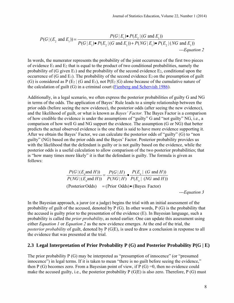
---Equation 2 In words, the numerator represents the probability of the joint occurrence of the first two pieces of evidence E1 and E2 that is equal to the product of two conditional probabilities, namely the probability of (G given E1) and the probability of the second evidence E2, conditional upon the occurrence of (G and E1). The probability of the second evidence E2 on the presumption of guilt (G) is considered as P (E2 | (G and E1), not P(E2 |G) alone because of the cumulative nature of the calculation of guilt (G) in a criminal court (Fienberg and Schervish 1986). Additionally, in a legal scenario, we often express the posterior probabilities of guilty G and NG in terms of the odds. The application of Bayes’ Rule leads to a simple relationship between the prior odds (before seeing the new evidence), the posterior odds (after seeing the new evidence), and the likelihood of guilt, or what is known as Bayes’ Factor. The Bayes Factor is a comparison of how credible the evidence is under the assumptions of “guilty” G and “not guilty” NG, i.e., a comparison of how well G and NG support the evidence. The assumption (G or NG) that better predicts the actual observed evidence is the one that is said to have more evidence supporting it. After we obtain the Bayes’ Factor, we can calculate the posterior odds of “guilty” (G) to “non guilty” (NG) based on the prior odds and the Bayes’ Factor. Posterior probability provides us with the likelihood that the defendant is guilty or is not guilty based on the evidence, while the posterior odds is a useful calculation to allow comparison of the two posterior probabilities; that is “how many times more likely” it is that the defendant is guilty. The formula is given as follows:

P(G | (Enand H ))

P(NG | (Enand H ))

P(G | H )

P(NG | H )

P(En

| (G and H ))

P(En

| (NG and H ))

(Posterior Odds) (Prior Odds) (Bayes Factor)

---Equation 3

In the Bayesian approach, a juror (or a judge) begins the trial with an initial assessment of the probability of guilt of the accused, denoted by P (G). In other words, P (G) is the probability that the accused is guilty prior to the presentation of the evidence (E). In Bayesian language, such a probability is called the prior probability, as noted earlier. One can update this assessment using either Equation 1 or Equation 2 as the new evidence emerges. At the end of the trial, the posterior probability of guilt, denoted by P (G|E), is used to draw a conclusion in response to all the evidence that was presented at the trial. 2.3 Legal Interpretation of Prior Probability P (G) and Posterior Probability P(G | E)

The prior probability P (G) may be interpreted as “presumption of innocence” (or “presumed innocence”) in legal terms. If it is taken to mean “there is no guilt before seeing the evidence,” then P (G) becomes zero. From a Bayesian point of view, if P (G) =0, then no evidence could make the accused guilty, i.e., the posterior probability P (G|E) is also zero. Therefore, P (G) must


9

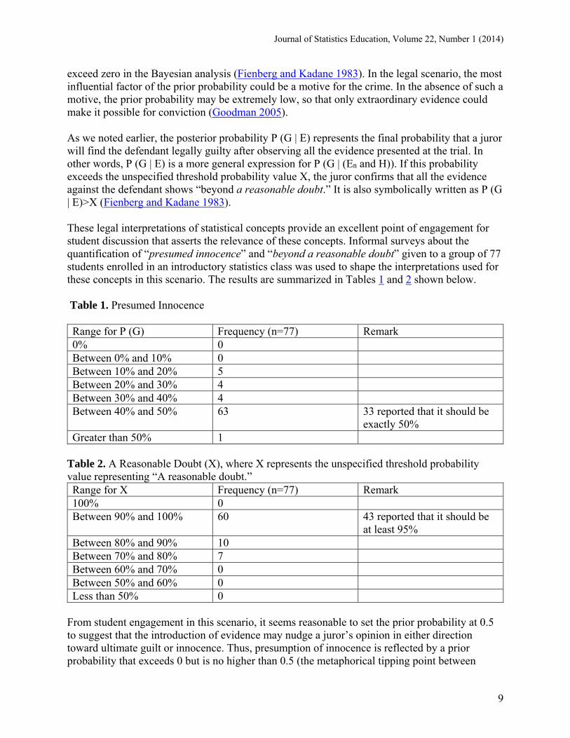
exceed zero in the Bayesian analysis (Fienberg and Kadane 1983). In the legal scenario, the most influential factor of the prior probability could be a motive for the crime. In the absence of such a motive, the prior probability may be extremely low, so that only extraordinary evidence could make it possible for conviction (Goodman 2005). As we noted earlier, the posterior probability P (G | E) represents the final probability that a juror will find the defendant legally guilty after observing all the evidence presented at the trial. In other words, P (G | E) is a more general expression for P (G | (En and H)). If this probability exceeds the unspecified threshold probability value X, the juror confirms that all the evidence against the defendant shows “beyond a reasonable doubt.” It is also symbolically written as P (G | E)>X (Fienberg and Kadane 1983). These legal interpretations of statistical concepts provide an excellent point of engagement for student discussion that asserts the relevance of these concepts. Informal surveys about the quantification of “presumed innocence” and “beyond a reasonable doubt” given to a group of 77 students enrolled in an introductory statistics class was used to shape the interpretations used for these concepts in this scenario. The results are summarized in Tables 1 and 2 shown below. Table 1. Presumed Innocence Range for P (G) Frequency (n=77) Remark 0% 0 Between 0% and 10% 0 Between 10% and 20% 5 Between 20% and 30% 4 Between 30% and 40% 4 Between 40% and 50% 63 33 reported that it should be

exactly 50% Greater than 50% 1

Table 2. A Reasonable Doubt (X), where X represents the unspecified threshold probability value representing “A reasonable doubt.” Range for X Frequency (n=77) Remark 100% 0 Between 90% and 100% 60 43 reported that it should be

at least 95% Between 80% and 90% 10 Between 70% and 80% 7 Between 60% and 70% 0 Between 50% and 60% 0 Less than 50% 0

From student engagement in this scenario, it seems reasonable to set the prior probability at 0.5 to suggest that the introduction of evidence may nudge a juror’s opinion in either direction toward ultimate guilt or innocence. Thus, presumption of innocence is reflected by a prior probability that exceeds 0 but is no higher than 0.5 (the metaphorical tipping point between


10

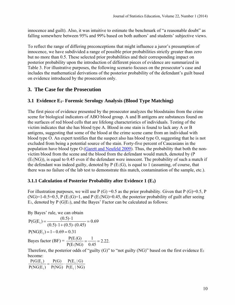
innocence and guilt). Also, it was intuitive to estimate the benchmark of “a reasonable doubt” as falling somewhere between 95% and 99% based on both authors’ and students’ subjective views. To reflect the range of differing preconceptions that might influence a juror’s presumption of innocence, we have subdivided a range of possible prior probabilities strictly greater than zero but no more than 0.5. These selected prior probabilities and their corresponding impact on posterior probability upon the introduction of different pieces of evidence are summarized in Table 3. For illustrative purposes, the following scenario focuses on the prosecutor’s case and includes the mathematical derivations of the posterior probability of the defendant’s guilt based on evidence introduced by the prosecution only. 3. The Case for the Prosecution 3.1 Evidence E1- Forensic Serology Analysis (Blood Type Matching) The first piece of evidence presented by the prosecutor analyzes the bloodstains from the crime scene for biological indicators of ABO blood group. A and B antigens are substances found on the surfaces of red blood cells that are lifelong characteristics of individuals. Testing of the victim indicates that she has blood type A. Blood in one stain is found to lack any A or B antigens, suggesting that some of the blood at the crime scene came from an individual with blood type O. An expert testifies that the suspect also has blood type O, suggesting that he is not excluded from being a potential source of the stain. Forty-five percent of Caucasians in the population have blood type O (Garett and Neufeld 2009). Thus, the probability that both the non-victim blood from the scene and the blood from the defendant would match, denoted by (P (E1|NG)), is equal to 0.45 even if the defendant were innocent. The probability of such a match if the defendant was indeed guilty, denoted by P (E1|G), is equal to 1 (assuming, of course, that there was no failure of the lab test to demonstrate this match, contamination of the sample, etc.). 3.1.1 Calculation of Posterior Probability after Evidence 1 (E1) For illustration purposes, we will use P (G) =0.5 as the prior probability. Given that P (G)=0.5, P (NG)=1-0.5=0.5, P (E1|G)=1, and P (E1|NG)=0.45, the posterior probability of guilt after seeing E1, denoted by P (G|E1), and the Bayes’ Factor can be calculated as follows: By Bayes’ rule, we can obtain

Bayes factor (BF) =

Therefore, the posterior odds of “guilty (G)” to “not guilty (NG)” based on the first evidence E1 become:

1

1

(0.5) 1P(G|E ) 0.69

(0.5) 1 (0.5) (0.45)

P(NG|E ) 1 0.69 0.31

1

1

P(E |G) 12.22.

P(E |NG) 0.45

1 1

1 1

P(G|E ) P(E | G)P(G)

P(NG|E ) P(NG) P(E | NG)


11

After the presentation of the first piece of evidence, E1, the probability of the defendant being guilty has increased from 0.5 to 0.69 (Table 3). Equivalently, the Bayes’ Factor

reveals that the credibility of E1 is 2.22 times greater under the

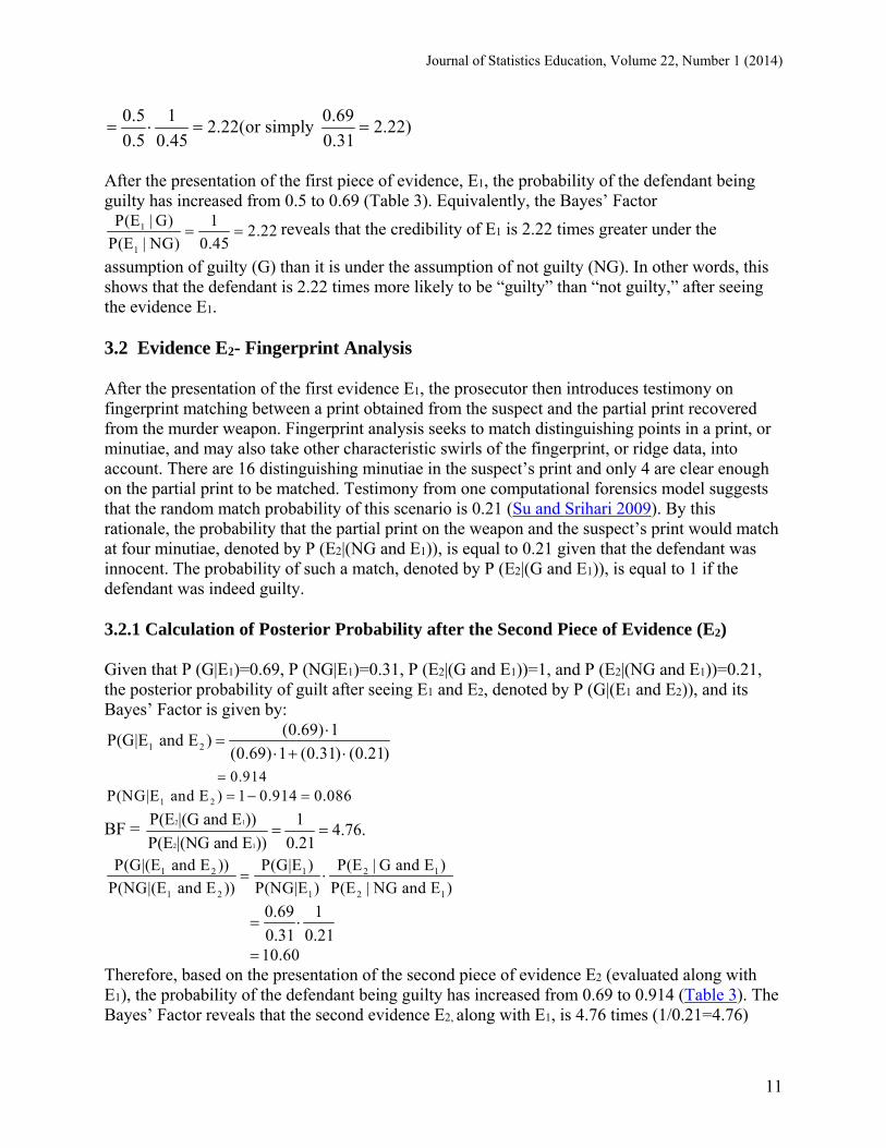
assumption of guilty (G) than it is under the assumption of not guilty (NG). In other words, this shows that the defendant is 2.22 times more likely to be “guilty” than “not guilty,” after seeing the evidence E1. 3.2 Evidence E2- Fingerprint Analysis After the presentation of the first evidence E1, the prosecutor then introduces testimony on fingerprint matching between a print obtained from the suspect and the partial print recovered from the murder weapon. Fingerprint analysis seeks to match distinguishing points in a print, or minutiae, and may also take other characteristic swirls of the fingerprint, or ridge data, into account. There are 16 distinguishing minutiae in the suspect’s print and only 4 are clear enough on the partial print to be matched. Testimony from one computational forensics model suggests that the random match probability of this scenario is 0.21 (Su and Srihari 2009). By this rationale, the probability that the partial print on the weapon and the suspect’s print would match at four minutiae, denoted by P (E2|(NG and E1)), is equal to 0.21 given that the defendant was innocent. The probability of such a match, denoted by P (E2|(G and E1)), is equal to 1 if the defendant was indeed guilty. 3.2.1 Calculation of Posterior Probability after the Second Piece of Evidence (E2) Given that P (G|E1)=0.69, P (NG|E1)=0.31, P (E2|(G and E1))=1, and P (E2|(NG and E1))=0.21, the posterior probability of guilt after seeing E1 and E2, denoted by P (G|(E1 and E2)), and its Bayes’ Factor is given by:

BF =

Therefore, based on the presentation of the second piece of evidence E2 (evaluated along with E1), the probability of the defendant being guilty has increased from 0.69 to 0.914 (Table 3). The Bayes’ Factor reveals that the second evidence E2, along with E1, is 4.76 times (1/0.21=4.76)

0.5 1 0.692.22(or simply 2.22)

0.5 0.45 0.31

1

1

P(E | G) 12.22

P(E | NG) 0.45

1 2

(0.69) 1P(G|E and E )

(0.69) 1 (0.31) (0.21)

0.914

1 2P(NG|E and E ) 1 0.914 0.086 2 1

2 1

P(E |(G and E )) 14.76.

P(E |(NG and E )) 0.21

1 2 1 2 1

1 2 1 2 1

P(G|(E and E )) P(G|E ) P(E | G and E )

P(NG|(E and E )) P(NG|E ) P(E | NG and E )

0.69 1

0.31 0.21

10.60


12

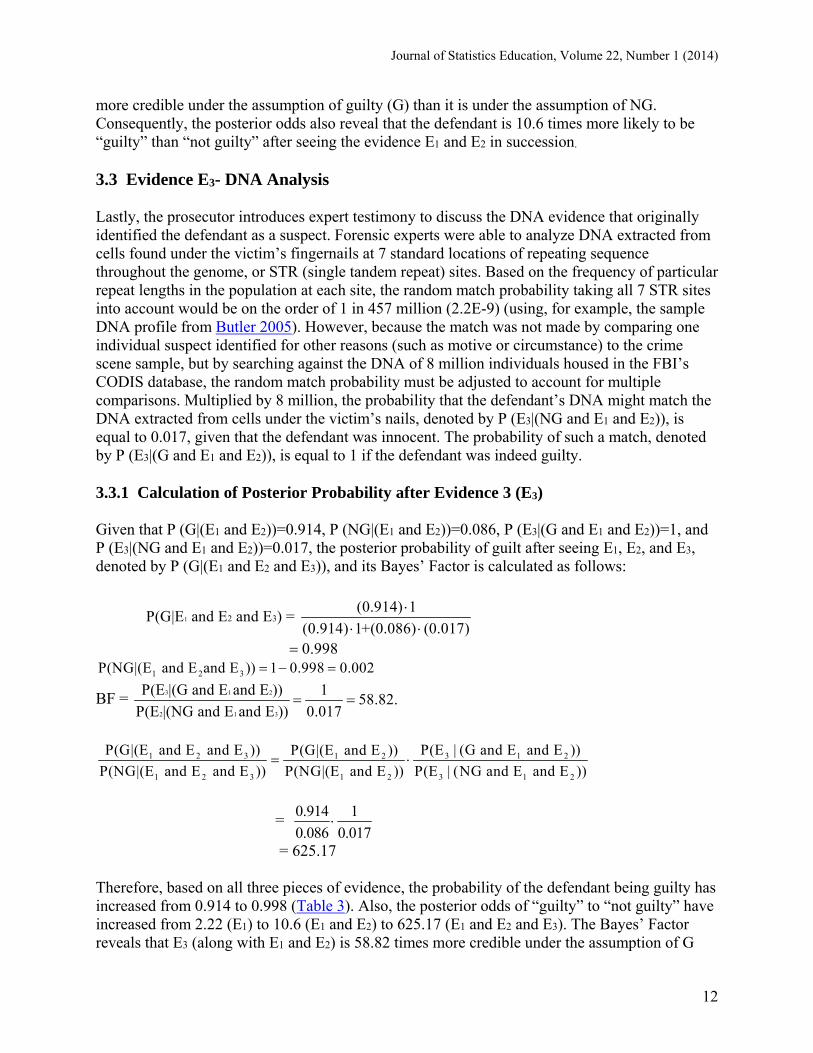
more credible under the assumption of guilty (G) than it is under the assumption of NG. Consequently, the posterior odds also reveal that the defendant is 10.6 times more likely to be “guilty” than “not guilty” after seeing the evidence E1 and E2 in succession. 3.3 Evidence E3- DNA Analysis Lastly, the prosecutor introduces expert testimony to discuss the DNA evidence that originally identified the defendant as a suspect. Forensic experts were able to analyze DNA extracted from cells found under the victim’s fingernails at 7 standard locations of repeating sequence throughout the genome, or STR (single tandem repeat) sites. Based on the frequency of particular repeat lengths in the population at each site, the random match probability taking all 7 STR sites into account would be on the order of 1 in 457 million (2.2E-9) (using, for example, the sample DNA profile from Butler 2005). However, because the match was not made by comparing one individual suspect identified for other reasons (such as motive or circumstance) to the crime scene sample, but by searching against the DNA of 8 million individuals housed in the FBI’s CODIS database, the random match probability must be adjusted to account for multiple comparisons. Multiplied by 8 million, the probability that the defendant’s DNA might match the DNA extracted from cells under the victim’s nails, denoted by P (E3|(NG and E1 and E2)), is equal to 0.017, given that the defendant was innocent. The probability of such a match, denoted by P (E3|(G and E1 and E2)), is equal to 1 if the defendant was indeed guilty. 3.3.1 Calculation of Posterior Probability after Evidence 3 (E3) Given that P (G|(E1 and E2))=0.914, P (NG|(E1 and E2))=0.086, P (E3|(G and E1 and E2))=1, and P (E3|(NG and E1 and E2))=0.017, the posterior probability of guilt after seeing E1, E2, and E3, denoted by P (G|(E1 and E2 and E3)), and its Bayes’ Factor is calculated as follows:

BF =

=

= 625.17 Therefore, based on all three pieces of evidence, the probability of the defendant being guilty has increased from 0.914 to 0.998 (Table 3). Also, the posterior odds of “guilty” to “not guilty” have increased from 2.22 (E1) to 10.6 (E1 and E2) to 625.17 (E1 and E2 and E3). The Bayes’ Factor reveals that E3 (along with E1 and E2) is 58.82 times more credible under the assumption of G

1 2 3(0.914) 1

P(G|E and E and E ) = (0.914) 1+(0.086) (0.017)

0.9981 2 3P(NG|(E and E and E )) 1 0.998 0.002

3 1 2

2 1 3

P(E |(G and E and E )) 158.82.

P(E |(NG and E and E )) 0.017

1 2 3 3 1 21 2

1 2 3 1 2 3 1 2

P(G|(E and E and E )) P(E | (G and E and E ))P(G|(E and E ))

P(NG|(E and E and E )) P(NG|(E and E )) P(E | (NG and E and E ))

0.914 1

0.086 0.017


13

than it is under the assumption of NG ( =58.82). The final piece of evidence E3 (DNA

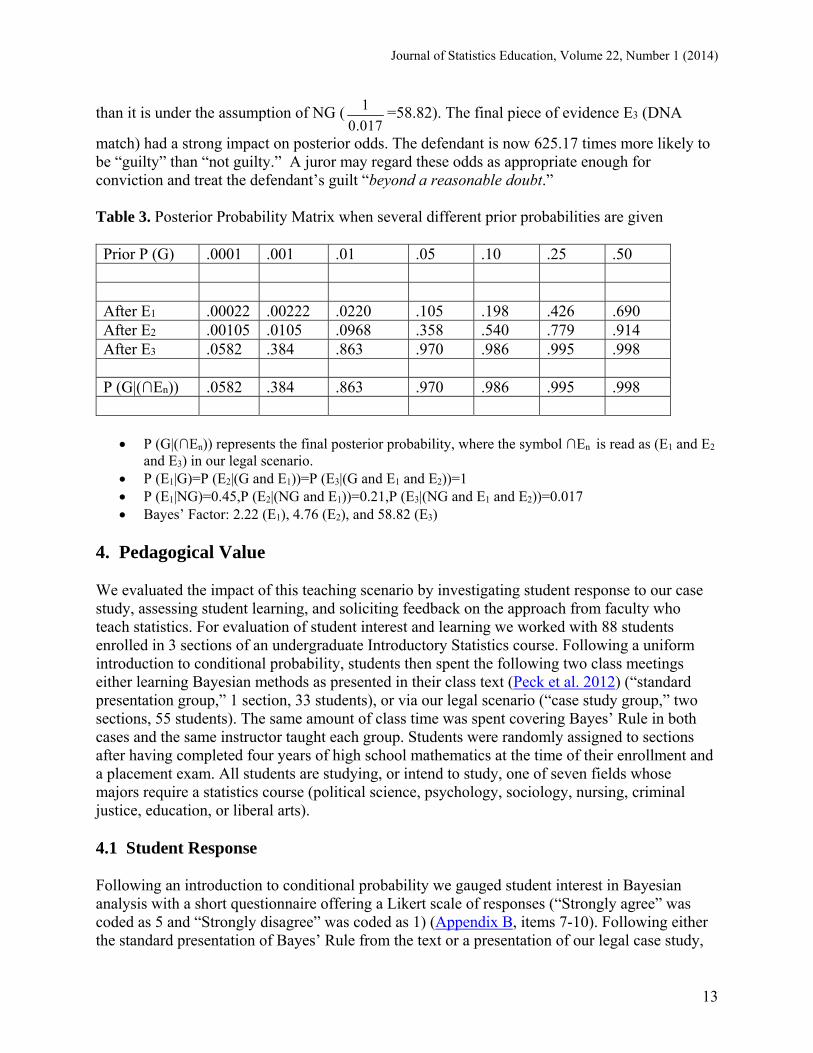
match) had a strong impact on posterior odds. The defendant is now 625.17 times more likely to be “guilty” than “not guilty.” A juror may regard these odds as appropriate enough for conviction and treat the defendant’s guilt “beyond a reasonable doubt.” Table 3. Posterior Probability Matrix when several different prior probabilities are given Prior P (G) .0001 .001 .01 .05 .10 .25 .50 After E1 .00022 .00222 .0220 .105 .198 .426 .690 After E2 .00105 .0105 .0968 .358 .540 .779 .914 After E3 .0582 .384 .863 .970 .986 .995 .998 P (G|(∩En)) .0582 .384 .863 .970 .986 .995 .998

P (G|(∩En)) represents the final posterior probability, where the symbol ∩En is read as (E1 and E2

and E3) in our legal scenario. P (E1|G)=P (E2|(G and E1))=P (E3|(G and E1 and E2))=1 P (E1|NG)=0.45,P (E2|(NG and E1))=0.21,P (E3|(NG and E1 and E2))=0.017 Bayes’ Factor: 2.22 (E1), 4.76 (E2), and 58.82 (E3)

4. Pedagogical Value We evaluated the impact of this teaching scenario by investigating student response to our case study, assessing student learning, and soliciting feedback on the approach from faculty who teach statistics. For evaluation of student interest and learning we worked with 88 students enrolled in 3 sections of an undergraduate Introductory Statistics course. Following a uniform introduction to conditional probability, students then spent the following two class meetings either learning Bayesian methods as presented in their class text (Peck et al. 2012) (“standard presentation group,” 1 section, 33 students), or via our legal scenario (“case study group,” two sections, 55 students). The same amount of class time was spent covering Bayes’ Rule in both cases and the same instructor taught each group. Students were randomly assigned to sections after having completed four years of high school mathematics at the time of their enrollment and a placement exam. All students are studying, or intend to study, one of seven fields whose majors require a statistics course (political science, psychology, sociology, nursing, criminal justice, education, or liberal arts). 4.1 Student Response Following an introduction to conditional probability we gauged student interest in Bayesian analysis with a short questionnaire offering a Likert scale of responses (“Strongly agree” was coded as 5 and “Strongly disagree” was coded as 1) (Appendix B, items 7-10). Following either the standard presentation of Bayes’ Rule from the text or a presentation of our legal case study,

1

0.017


14

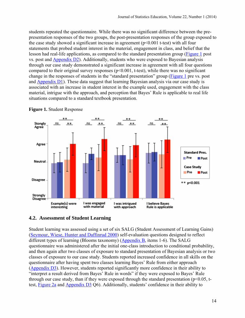
students repeated the questionnaire. While there was no significant difference between the pre-presentation responses of the two groups, the post-presentation responses of the group exposed to the case study showed a significant increase in agreement (p<0.001 t-test) with all four statements that probed student interest in the material, engagement in class, and belief that the lesson had real-life applications, as compared to the standard presentation group (Figure 1 post vs. post and Appendix D2). Additionally, students who were exposed to Bayesian analysis through our case study demonstrated a significant increase in agreement with all four questions compared to their original survey responses (p<0.001, t-test), while there was no significant change in the responses of students in the “standard presentation” group (Figure 1 pre vs. post and Appendix D1). These data suggest that learning Bayesian analysis via our case study is associated with an increase in student interest in the example used, engagement with the class material, intrigue with the approach, and perception that Bayes’ Rule is applicable to real life situations compared to a standard textbook presentation. Figure 1. Student Response

4.2. Assessment of Student Learning Student learning was assessed using a set of six SALG (Student Assessment of Learning Gains) (Seymour, Wiese, Hunter and Daffinrud 2000) self-evaluation questions designed to reflect different types of learning (Blooms taxonomy) (Appendix B, items 1-6). The SALG questionnaire was administered after the initial one-class introduction to conditional probability, and then again after two classes of exposure to standard presentation of Bayesian analysis or two classes of exposure to our case study. Students reported increased confidence in all skills on the questionnaire after having spent two classes learning Bayes’ Rule from either approach (Appendix D3). However, students reported significantly more confidence in their ability to “interpret a result derived from Bayes’ Rule in words” if they were exposed to Bayes’ Rule through our case study, than if they were exposed through the standard presentation (p<0.05, t-test, Figure 2a and Appendix D3 Q6). Additionally, students’ confidence in their ability to


15

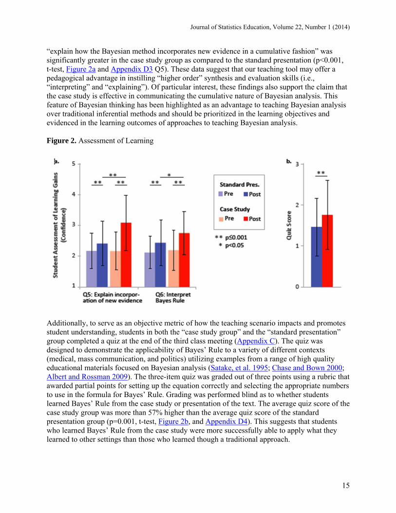
“explain how the Bayesian method incorporates new evidence in a cumulative fashion” was significantly greater in the case study group as compared to the standard presentation (p<0.001, t-test, Figure 2a and Appendix D3 Q5). These data suggest that our teaching tool may offer a pedagogical advantage in instilling “higher order” synthesis and evaluation skills (i.e., “interpreting” and “explaining”). Of particular interest, these findings also support the claim that the case study is effective in communicating the cumulative nature of Bayesian analysis. This feature of Bayesian thinking has been highlighted as an advantage to teaching Bayesian analysis over traditional inferential methods and should be prioritized in the learning objectives and evidenced in the learning outcomes of approaches to teaching Bayesian analysis. Figure 2. Assessment of Learning

Additionally, to serve as an objective metric of how the teaching scenario impacts and promotes student understanding, students in both the “case study group” and the “standard presentation” group completed a quiz at the end of the third class meeting (Appendix C). The quiz was designed to demonstrate the applicability of Bayes’ Rule to a variety of different contexts (medical, mass communication, and politics) utilizing examples from a range of high quality educational materials focused on Bayesian analysis (Satake, et al. 1995; Chase and Bown 2000; Albert and Rossman 2009). The three-item quiz was graded out of three points using a rubric that awarded partial points for setting up the equation correctly and selecting the appropriate numbers to use in the formula for Bayes’ Rule. Grading was performed blind as to whether students learned Bayes’ Rule from the case study or presentation of the text. The average quiz score of the case study group was more than 57% higher than the average quiz score of the standard presentation group (p=0.001, t-test, Figure 2b, and Appendix D4). This suggests that students who learned Bayes’ Rule from the case study were more successfully able to apply what they learned to other settings than those who learned though a traditional approach.


16

4.3. Faculty Feedback The case study approach was presented to a group of mathematics and statistics instructors at a local four-year state college who have taught statistics and/or biostatistics. These faculty pointed out the appeal of using a realistic scenario with parallels to criminal cases seen on TV (such as on Dateline, 20/20, etc.). Faculty appreciated the logic of using DNA evidence to engage students while also aiming to rectify common misconceptions about DNA forensic evidence. They commented that, in comparison to the standard approach, the case scenario highlights how Bayes’ Rule works in a cumulative, not a terminal, way. “We can see how largely the various different prior probabilities influence their posterior probabilities,” said one faculty member, while another faculty member commented on how the case clearly illustrated the usefulness of Bayes’ Rule in calculating the posterior probability of a complex problem. The complexity of the type of problem to which Bayes’ Rule is applied was a source of criticism from one faculty member, who rejected the underlying premise that Bayesian analysis ought to be approached in an introductory statistics course. While the teaching scenario positively impacted student learning by both metrics above, we acknowledge that even the improved student understanding was not at an ideal level on this topic. We attribute these findings in part to the fact that Bayes’ Rule is a complex topic and that the three class meetings utilized for this study are not enough to reasonably expect its mastery. All mathematics and statistics faculty members who were open to teaching Bayesian thinking at an introductory level, were enthusiastic about an approach that sought to connect to real life examples and make the approach relevant. “It is intellectually challenging and stimulating in every aspect,” concluded one faculty member. 5. Conclusion Despite the fact that the discipline of statistics remains healthy, Moore (1997) has opined that its place in academe is not. In relation to Moore’s comment on undergraduate statistics curriculum, Bolstad (2002) suggested that Bayesian methods may be the key to revitalizing our undergraduate programs in statistics. Additionally, Albert, Berry, Rossman, and others encourage instructors to implement Bayesian thinking into the elementary statistical inference and decision-making process (Albert 1995; Berry 1996; Albert and Rossman 2009). However, in most universities and colleges, exposure to Bayesian statistics in the current undergraduate statistics curriculum is very limited. Winkler (2001) gave a detailed list of the recommendations on “how to promote Bayesian methods in basic courses.” He suggested that more materials should be developed for Bayesian training in basic courses, including more basic texts written for a Bayesian perspective (e.g., Berry 1996; Albert and Rossman 2009) and easier-to-use Bayesian software for students and practitioners (e.g., Albert 1996). He also emphasized the importance of “training the trainers” to increase the awareness of the importance and practical applications of Bayesian methods at the introductory and intermediate levels. He suggested that instructors of basic statistics courses must understand the fundamentals of Bayesian methods first to teach the material most effectively. The present work responds to the latter of these recommendations by demonstrating the teaching scenario to the instructors of mathematics and statistics and engaging this group in dialogue about the approach.


17

The teaching scenario illustrated in this paper is intended to be complementary to existing strategies for teaching Bayesian thinking that aim to make Bayes’ Rule relevant and accessible. For example, the innovative work of Albert and Rossman’s Workshop textbook also uses a courtroom forensics example in Activity 15/15 (Albert and Rossman 2009). This teaching scenario utilizes the engaging courtroom context to highlight the cumulative nature of Bayes’ Rule by introducing several rounds of evidence of increasing strength. It also includes an empirical assessment of effectiveness that supports its success in highlighting this aspect of Bayes’ Rule and its positive impact on student engagement and learning in comparison to a standard textbook treatment. This approach also represents a teaching-focused illustration of the application of Bayes’ Rule to evaluating guilt or innocence in a court case. This application of Bayes’ Rule was noted in the 1983 work of Fienberg and Kadane. We adapt Fienberg and Kadane’s observations to the classroom and evaluate student learning quantitatively. Further, our work updates and expands upon such work by integrating modern forensic evidence, including DNA analysis. Even as DNA analysis has been held up as the gold standard for rigorous and consistent support of conclusions about individualization, there are numerous ways that DNA evidence can be and has been misused (Murphy 2009). The perceived infallibility of DNA evidence extends beyond the courtroom and becomes an idea entrenched in both academic circles and popular culture (Thompson 2006). A troubling effect of such attitudes may be a failure to question any DNA-based information, whether it is delivered to someone as a juror, or as a consumer of the media, or as a patient in a medical situation. The teaching scenario illustrated here provides a crucial opportunity for impacting such societal misconceptions by discussing the nature of the DNA evidence presented. Students can be guided to explore the mathematical arguments utilized to determine the particular prior probability used for the DNA evidence and discuss how different handling of the DNA evidence or testimony would affect this value. They can determine the important questions to ask for critical evaluation of DNA information and gain an appreciation for how a lack of awareness about such factors could lead to misuses or misunderstandings about the meaning of statistical arguments commonly made about the uniqueness of DNA in the courtroom and in other contexts. Lastly, the scenario also showed us that probabilities of guilt fluctuate to a smaller or larger extent, contingent upon the strength of evidence. This means, as the strength of the evidence increases for the defendant’s status of guilt, the data are more able to convert a skeptic into a believer of the claim “the defendant is guilty.” Furthermore, the manner in which the posterior probabilities of guilt are determined appears to favor a Bayesian rather than a classical statistics approach. In classical statistics, each event is treated independently with a p-value and/or α value to determine its statistical significance. The methodology used in classical statistics is not designed to consider and further calculate influencing factors that precede an event. Bayesian statistical methods, on the other hand, are designed to determine and evaluate phenomena by revising and updating probabilities in light of current and prior events (Satake 1994). Regardless of the debate as to what approach to take in legal decision-making processes, the teaching of Bayes’ Rule within a course in introductory statistics has much to offer, particularly in light of the growing interest in Bayesian statistics as a research instrument in a wide range of disciplines and professions, especially those involved in and closely related to decision-making processes.


18

Such applications have made many statistics educators aware that the Bayesian perspective should be emphasized more in introductory statistics courses to help students develop both deductive (general to specific) and inductive (specific to general) statistical reasoning, which are the essential components of statistical inference. The Bayesian perspective can also deepen students’ general knowledge about the subject matter of probability and statistical inference.

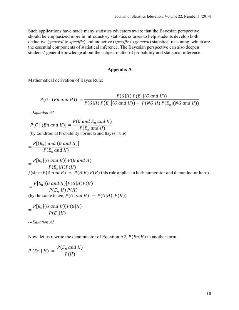
Appendix A Mathematical derivation of Bayes Rule:

| | |

| | |

---Equation A1

|

byConditionalProbabilityFormulaandBayes’rule

|

|

| since | thisruleappliestobothnumeratoranddenominatorhere

| |

|

bythesametoken, |

| ||

---Equation A2

Now, let us rewrite the denominator of Equation A2, | in another form.

|


19

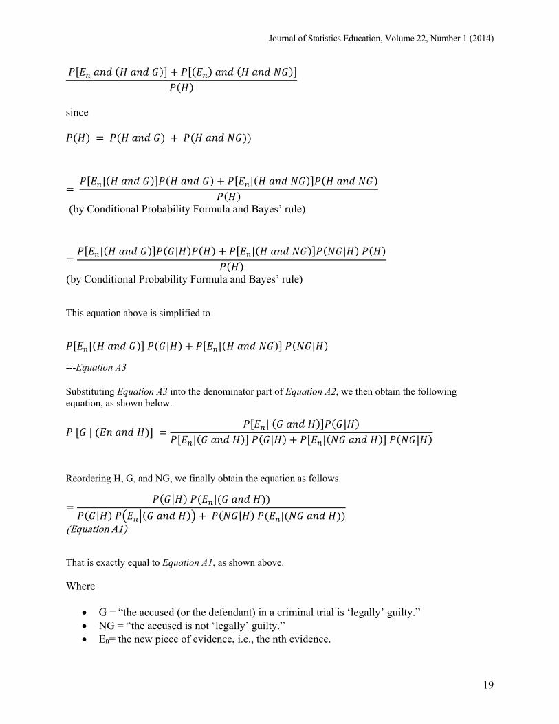
since

| |

by Conditional Probability Formula and Bayes’ rule)

| | | |

by Conditional Probability Formula and Bayes’ rule)

This equation above is simplified to

| | | |

---Equation A3 Substituting Equation A3 into the denominator part of Equation A2, we then obtain the following equation, as shown below.

| | |

| | | |

Reordering H, G, and NG, we finally obtain the equation as follows.

| |

| | |

EquationA1

That is exactly equal to Equation A1, as shown above. Where

G = “the accused (or the defendant) in a criminal trial is ‘legally’ guilty.” NG = “the accused is not ‘legally’ guilty.” En= the new piece of evidence, i.e., the nth evidence.


20

H = all of the evidence presented up to a certain point (prior to the presentation of the new evidence) in the trial. H is also symbolically expressed as follows:

H = ⋂ …

| the probability of G, given the evidence H. This probability is termed as the prior probability (at a point H is already presented) in the Bayesian language.

theprobabilitythatmeasuresthecredibilityoftheevidenceEnbasedon thepresumptionofguiltyand theevidenceH. In forensicevidence, thiscredibilityisintimatelyrelatedtotherarityofaparticularpieceofevidence.

| theprobabilityofinnocence “legally”notguilty ,giventheevidenceH.Itisalsocalculatedby1 |

the probability that measures the credibility of the evidence En based on the presumption of innocence and the evidence H. It is also calculated by 1 |

the probability of G given all evidence up to and including En. This probability is termed as the posterior probability (at a point H and En are already presented) in the Bayesian language.

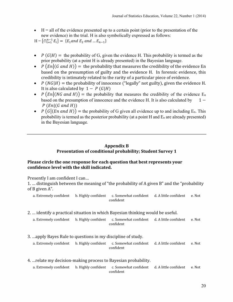
AppendixBPresentationofconditionalprobability;StudentSurvey1

Pleasecircletheoneresponseforeachquestionthatbestrepresentsyourconfidencelevelwiththeskillindicated.PresentlyIamconfidentIcan…1.…distinguishbetweenthemeaningof“theprobabilityofAgivenB”andthe“probabilityofBgivenA”.

a.Extremelyconfidentb.Highlyconfidentc.Somewhatconfidentd.Alittleconfidente.Notconfident

2.…identifyapracticalsituationinwhichBayesianthinkingwouldbeuseful.a.Extremelyconfidentb.Highlyconfidentc.Somewhatconfidentd.Alittleconfidente.Not

confident

3.…applyBayesRuletoquestionsinmydisciplineofstudy.a.Extremelyconfidentb.Highlyconfidentc.Somewhatconfidentd.Alittleconfidente.Not

confident

4.…relatemydecision‐makingprocesstoBayesianprobability.a.Extremelyconfidentb.Highlyconfidentc.Somewhatconfidentd.Alittleconfidente.Not

confident


21

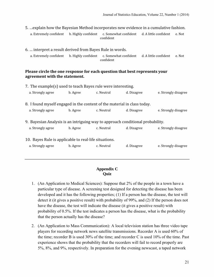
5.…explainhowtheBayesianMethodincorporatesnewevidenceinacumulativefashion.a.Extremelyconfidentb.Highlyconfidentc.Somewhatconfidentd.Alittleconfidente.Not

confident

6.…interpretaresultderivedfromBayesRuleinwords.a.Extremelyconfidentb.Highlyconfidentc.Somewhatconfidentd.Alittleconfidente.Not

confident

Pleasecircletheoneresponseforeachquestionthatbestrepresentsyouragreementwiththestatement.7.Theexample(s)usedtoteachBayesrulewereinteresting.a.Stronglyagreeb.Agreec.Neutrald.Disagreee.Stronglydisagree

8.Ifoundmyselfengagedinthecontentofthematerialinclasstoday.a.Stronglyagreeb.Agreec.Neutrald.Disagreee.Stronglydisagree

9.BayesianAnalysisisanintriguingwaytoapproachconditionalprobability.a.Stronglyagreeb.Agreec.Neutrald.Disagreee.Stronglydisagree

10.BayesRuleisapplicabletoreal‐lifesituations.a.Stronglyagreeb.Agreec.Neutrald.Disagreee.Stronglydisagree

Appendix C Quiz

1. (An Application to Medical Sciences): Suppose that 2% of the people in a town have a

particular type of disease. A screening test designed for detecting the disease has been developed and it has the following properties; (1) If a person has the disease, the test will detect it (it gives a positive result) with probability of 99%, and (2) If the person does not have the disease, the test will indicate the disease (it gives a positive result) with probability of 0.5%. If the test indicates a person has the disease, what is the probability that the person actually has the disease?

2. (An Application to Mass Communication): A local television station has three video tape players for recording network news satellite transmissions. Recorder A is used 60% of the time; recorder B is used 30% of the time; and recorder C is used 10% of the time. Past experience shows that the probability that the recorders will fail to record properly are 5%, 8%, and 9%, respectively. In preparation for the evening newscast, a taped network


22

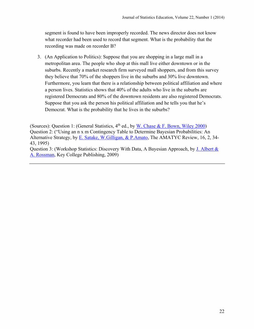
segment is found to have been improperly recorded. The news director does not know what recorder had been used to record that segment. What is the probability that the recording was made on recorder B?

3. (An Application to Politics): Suppose that you are shopping in a large mall in a metropolitan area. The people who shop at this mall live either downtown or in the suburbs. Recently a market research firm surveyed mall shoppers, and from this survey they believe that 70% of the shoppers live in the suburbs and 30% live downtown. Furthermore, you learn that there is a relationship between political affiliation and where a person lives. Statistics shows that 40% of the adults who live in the suburbs are registered Democrats and 80% of the downtown residents are also registered Democrats. Suppose that you ask the person his political affiliation and he tells you that he’s Democrat. What is the probability that he lives in the suburbs?

(Sources): Question 1: (General Statistics, 4th ed., by W. Chase & F. Bown, Wiley 2000) Question 2: (“Using an n x m Contingency Table to Determine Bayesian Probabilities: An Alternative Strategy, by E. Satake, W.Gilligan, & P.Amato, The AMATYC Review, 16, 2, 34-43, 1995) Question 3: (Workshop Statistics: Discovery With Data, A Bayesian Approach, by J. Albert & A. Rossman, Key College Publishing, 2009)


23

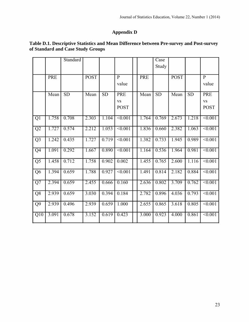
Appendix D Table D.1. Descriptive Statistics and Mean Difference between Pre-survey and Post-survey of Standard and Case Study Groups

Standard CaseStudy

PRE POST P value

PRE POST P value

Mean SD Mean SD PREvs POST

Mean SD Mean SD PREvs POST

Q1 1.758 0.708 2.303 1.104 <0.001 1.764 0.769 2.673 1.218 <0.001

Q2 1.727 0.574 2.212 1.053 <0.001 1.836 0.660 2.382 1.063 <0.001

Q3 1.242 0.435 1.727 0.719 <0.001 1.382 0.733 1.945 0.989 <0.001

Q4 1.091 0.292 1.667 0.890 <0.001 1.164 0.536 1.964 0.981 <0.001

Q5 1.458 0.712 1.758 0.902 0.002 1.455 0.765 2.600 1.116 <0.001

Q6 1.394 0.659 1.788 0.927 <0.001 1.491 0.814 2.182 0.884 <0.001

Q7 2.394 0.659 2.455 0.666 0.160 2.636 0.802 3.709 0.762 <0.001

Q8 2.939 0.659 3.030 0.394 0.184 2.782 0.896 4.036 0.793 <0.001

Q9 2.939 0.496 2.939 0.659 1.000 2.655 0.865 3.618 0.805 <0.001

Q10 3.091 0.678 3.152 0.619 0.423 3.000 0.923 4.000 0.861 <0.001


24

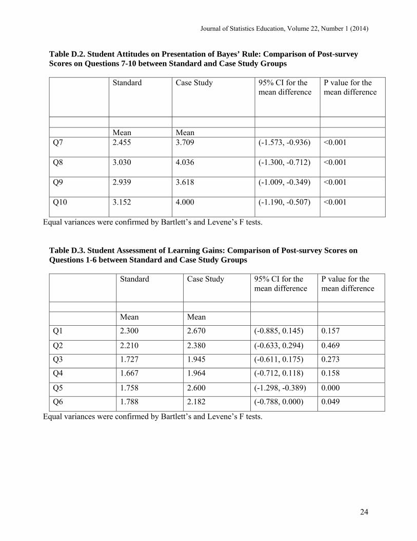
Table D.2. Student Attitudes on Presentation of Bayes’ Rule: Comparison of Post-survey Scores on Questions 7-10 between Standard and Case Study Groups Standard Case Study 95% CI for the

mean difference P value for the mean difference

Mean Mean Q7 2.455 3.709 (-1.573, -0.936) <0.001

Q8 3.030 4.036 (-1.300, -0.712) <0.001

Q9 2.939 3.618 (-1.009, -0.349) <0.001

Q10 3.152 4.000 (-1.190, -0.507) <0.001

Equal variances were confirmed by Bartlett’s and Levene’s F tests. Table D.3. Student Assessment of Learning Gains: Comparison of Post-survey Scores on Questions 1-6 between Standard and Case Study Groups Standard Case Study 95% CI for the

mean difference P value for the mean difference

Mean Mean

Q1 2.300 2.670 (-0.885, 0.145) 0.157

Q2 2.210 2.380 (-0.633, 0.294) 0.469

Q3 1.727 1.945 (-0.611, 0.175) 0.273

Q4 1.667 1.964 (-0.712, 0.118) 0.158

Q5 1.758 2.600 (-1.298, -0.389) 0.000

Q6 1.788 2.182 (-0.788, 0.000) 0.049

Equal variances were confirmed by Bartlett’s and Levene’s F tests.


25

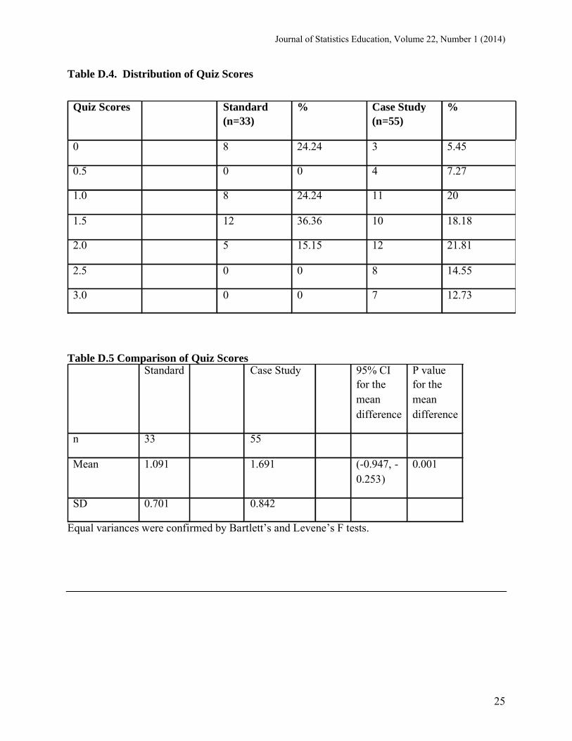
Table D.4. Distribution of Quiz Scores

Table D.5 Comparison of Quiz Scores

Standard Case Study 95% CI for the mean difference

P value for the mean difference

n 33 55

Mean 1.091 1.691 (-0.947, -0.253)

0.001

SD 0.701 0.842

Equal variances were confirmed by Bartlett’s and Levene’s F tests.

Quiz Scores Standard(n=33)

% Case Study (n=55)

%

0 8 24.24 3 5.45

0.5 0 0 4 7.27

1.0 8 24.24 11 20

1.5 12 36.36 10 18.18

2.0 5 15.15 12 21.81

2.5 0 0 8 14.55

3.0 0 0 7 12.73


26

References Agresti, A., and Franklin, C. (2012), The Art and Science of Learning from Data, New York, NY: Addison Wesley. Albert, J. (1993), "Teaching Bayesian Statistics Using Sampling Methods in Minitab," The American Statistician, 47, 182-191. Albert, J. (1995), "Teaching Inference About Proportions Using Bayes and Discrete Models," The Journal of Statistics Education, 3, http://www.amstat.org/publications/jse/v3n3/albert.html. Albert, J. (1996), Bayesian Computation Using Minitab, Boston: Duxbury Press. Albert, J. H., and Rossman, A. J. (2009), Workshop Statistics: Discovery with Data, a Bayesian Approach, Key College Publishing. Ashby, D. (2006), "Bayesian Statistics in Medicine: A 25-Year Review," Statistics in Medicine, 25, 3589–3631. Berry, D. (1996), Statistics: A Bayesian Perspective, Belmont, CA: Wadsworth. Bolstad, W. M. (2002), "Teaching Bayesian Statistics to Undergraduates: Who, What, Where, When, Why and How," in ICOTS6 International Conference on Teaching Statistics, Capetown, South Africa. Boster, F. J., Hunter, J. E., and Hale, J. L. (1991), "An Information-Processing Model of Jury Decision-Making," Communication Research, 18, 524-547. Butler, J. M. (2005), "Profile Frequency Estimates, Likelihood Ratios, and Source Attribution," in Forensic DNA Typing: Biology, Technology, and Genetics of Str Markers (2 ed.), pp. 497-517. Chase, W., and Bown, F. (2000), General Statistics (4 ed.), New York, NY: Wiley. Davis, J. H., Bray, R. M., and Holt, R. (1977), "The Empirical Study of Social Decision Processes in Juries," in Law, Justice, and the Individual in Society: Psychological and Legal Perspectives, eds. J. Tapp and F. Levine, New York, NY: Holt, Rinehart, and Winston. De Veaux, R. D., Velleman, P. F., and Bock, D. E. (2008), Stats Data and Models (2 ed.), Boston, MA: Pearson-Addison Wesley. Fienberg, S. E., and Kadane, J. B. (1983), "The Presentation of Bayesian Statistical Analyses in Legal Proceedings," The Statistician, 32, 88-98. Fienberg, S. E., and Schervish, M. J. (1986), "The Relevance of Bayesian Inference for the Presentation of Statistical Evidence and for Legal-Decision-Making," Boston University Law Review, 66, 771-788.


27

Finkelstein, M. O. (1978), Quantitative Methods in Law: Studies in the Application of Mathematical Probability and Statistics to Legal Problems, New York, NY: The Free Press. Finkelstein, M. O., and Fairley, W. B. (1970), "A Bayesian Approach to Identification of Evidence," Harvard Law Review, 83, 489-517. Garett, B. L., and Neufeld, P. J. (2009), "Invalid Forensic Science Testimony and Wrongful Convinctions," Virginia Law Review, 95, 1-97. Gelfand, A. E., and Solomon, H. A. (1973), "A Study of Poisson’s Models for Jury Verdict in Criminal and Civil Trials," Journal of the American Statistical Association, 68, 241-278. Gelfand, A. E., and Solomon, H. A. (1974), "Modeling Jury Verdicts in the American Legal System," Journal of the American Statistical Association, 69, 32-37. Gelfand, A. E., and Solomon, H. A. (1975), "Analyzing the Decision-Making Process of the American Jury," Journal of the American Statistical Association, 70, 305-309. Goodman, S. (1999), "Towards Evidence-Based Medical Statistics, 2: The Bayes Factor," Annals of Internal Medicine, 130, 1005-1013. Goodman, S. (2005), "Judgment for Judges: What Traditional Statistics Don't Tell You About Causal Claims," Brooklyn Law School Review, 15. Haigh, J. (2003), Taking Chances : Winning with Probability, New York, NY: Oxford University Press. Iversen, G. R. (1984), Bayesian Statistical Inference, Newbury Park, CA: Sage Publications. Lindley, D. L. (1977), "Probability and the Law," Journal of the Royal Statistics Society, 26, 203-220. Marshall, C. R., and Wise, J. A. (1975), "Juror Decisions and the Determination of Guilt in Capital Punishment Cases: A Bayesian Perspective," in Utility, Probability, and Human Decision-Making, eds. D. Wendt and C. Vlek, Dordrecht, Holland: Reidel. Maxwell, L. D., and Satake, E. (2010), "Scientific Literacy and Ethical Pratice: Time for a Check-Up," Annual Amercan Speech-Language-Hearing Association Convention Moore, D. S. (1997), "Bayes for Beginners? Some Reasons to Hesitate," The American Statistician, 51, 254-261. Murphy, E. (2009), "The Art in the Science of DNA: A Layperson’s Guide to the Subjectivity Inherent in Forensic DNA Typing," Emory Law Journal, 58, 489-495.


28

Ostrom, T. M., Werner, C., and Saks, M. J. (1978), "An Integration Theory Analysis of Jurors’ Presumption of Guilt or Innocence," Journal of Personality and Social Psychology, 36, 436-450. Peck, R. L., Olsen, C., and Devore, J. L. (2012), Introduction to Statistics and Data Analysis (4 ed.), Boston, MA: Brooks/Cole. Pennington, N., and Hastie, R. (1981), "Juror Decision-Making Models: The Generalization Gap," Psychological Bulletin, 89, 246-287. Penrod, S., and Hastie, R. (1979), "Models of Jury Decision-Making: A Critical Review," Psychological Bulletin, 86, 462-492. Pfenning, N. (2011), Elementary Statistics: Looking at the Big Picture, Boston, MA: Brooks/Cole. Poisson, S. D. (1837), Recherches Sur La Probabilite Des Jugements En Matiere Criminelle Et En Matiere Civile, Paris, France: Bachelier, Imprimeur-Lobrairie. Polya, G. (1954), Mathematics and Plausible Reasoning: Patterns of Plausible Inference, Princeton, NJ: Princeton University Press. Rossman, A. J., and Short, T. H. (1995), "Conditional Probability and Education Reform: Are They Compatible?," Journal of Statistics Education, 3, http://www.amstat.org/publications/jse/v3n2/rossman.html. Saks, M. J., and Ostrom, T. M. (1975), "Jury Size and Consensus Requirements: The Laws of Probability V. The Laws of the Land," Journal of Contemporary Law, 1, 163-173. Satake, E. (1994), "Bayesian Inference in Polling Technique: 1992 Presidential Polls," Communication Research, 21, 396-407. Satake, E., and Amato, P. P. (1999), "Probability and Law: A Bayesian Approach," in The Bulletin of International Statistics Instistute 52nd Session, Helsinki, FInland. Satake, E., and Amato, P. P. (2008), "An Alternative Version of Conditional Probabilities and Bayes’ Rule: An Application of Probability Logic," The AMATYC Review, 29, 44-50. Satake, E., Gilligan, W., and Amato, P. (1995), "Using an N X M Contingency Table to Determine Bayesian Probabilities: An Alternative Strategy," The AMATYC Review, 16, 34-43. Schum, D. A. (1975), "The Weighing of Testimony in Judicial Proceedings from Sources Having Reduced Credibility," Human Factors, 17, 172-182. Seymour, E., Wiese, D., Hunter, A., and Daffinrud, S. M. (2000), "Creating a Better Mousetrap: On-Line Student Assessment of Their Learning Gains.," National Meeting of the American Chemical Society.


29

Strengthening Forensic Science in the United States: A Path Forward (2009), The National Academies Press. Su, C., and Srihari, S. N. (2009), "Probability of Random Correspondence for Fingerprints," in Computational Forensics (Vol. 5718), eds. Z. J. M. H. Geradts, K. Y. Franke and C. J. Veenman, Springer Berlin Heidelberg, pp. 55-66. Thomas, E. A., and Hogue, A. (1976), "Apparent Weight of Evidence, Decision Criteria, and Confidence Ratings in Juror Decision-Making," Psychological Review, 83, 442-465. Thompson, W. C. (2006), "Tarnish on the ‘Gold Standard’: Recent Problems in Forensic DNA Testing," The National Association of Criminal Defense Lawyers Champion Magazine, 10-19. Utts, J. M., and Heckard, R. F. (2011), Mind on Statistics (4 ed.), Boston, MA: Brooks/Cole. Walbert, T. D. (1971), "Effect of Jury Size on Probability of Conviction: An Evaluation of Williams V. Florida," Case Western Reserve Law Review, 22, 529-555. Winkler, R. L. (2001), "Why Bayesian Analysis Hasn’t Caught on in Healthcare Decision-Making," International Journal of Technology Assessment in Health Care, 17, 56-66. Eiki Satake Department of Communication Sciences and Disorders Emerson College 180 Boylston Street Boston MA, 02116 Mailto: [email protected] Amy Vashlishan Murray Department of Communication Sciences and Disorders Emerson College 180 Boylston Street Boston MA, 02116 Mailto: [email protected]

Volume 22 (2014) | Archive | Index | Data Archive | Resources | Editorial Board | Guidelines for Authors | Guidelines for Data Contributors | Guidelines for Readers/Data Users | Home Page |

Contact JSE | ASA Publications

Documents

Teaching an Application of Bayes’ Rule for Legal Decision ...jse.amstat.org/v22n1/satake.pdf · Bayes' Rule, and utilize Bayes’ Factor in the computation process to further promote