Embed Size (px)
Citation preview
10th Madrid Summer School on Advanced Statistics and Data Mining
!Module C9 :: Text Mining 6th July - 10th of July 2015
!Florian Leitner
License:
Text Mining 1 Introduction
!Madrid Summer School on
Advanced Statistics and Data Mining !
Florian Leitner [email protected]
License:
Florian Leitner <[email protected]> MSS/ASDM: Text Mining
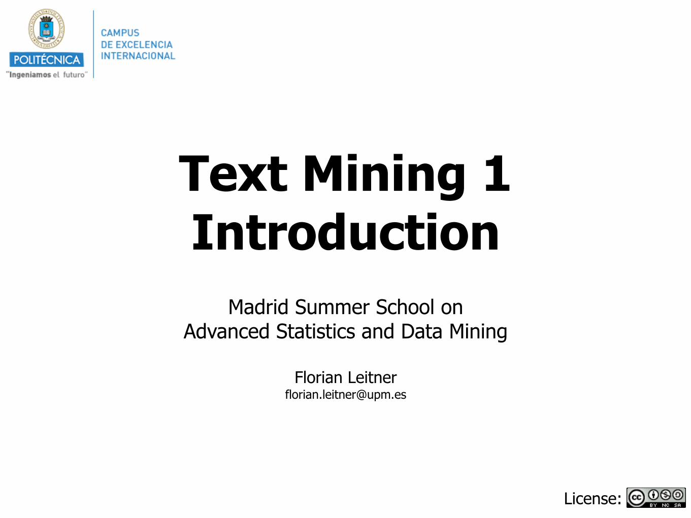
“Text mining” or“text analytics”
The discovery of new or existing facts from text by applying natural language processing (NLP), statistical learning techniques, or both.
3
Machine Learning
Inferential Statistics
Computat. Linguistics RulesModels
Predictions
Florian Leitner <[email protected]> MSS/ASDM: Text Mining
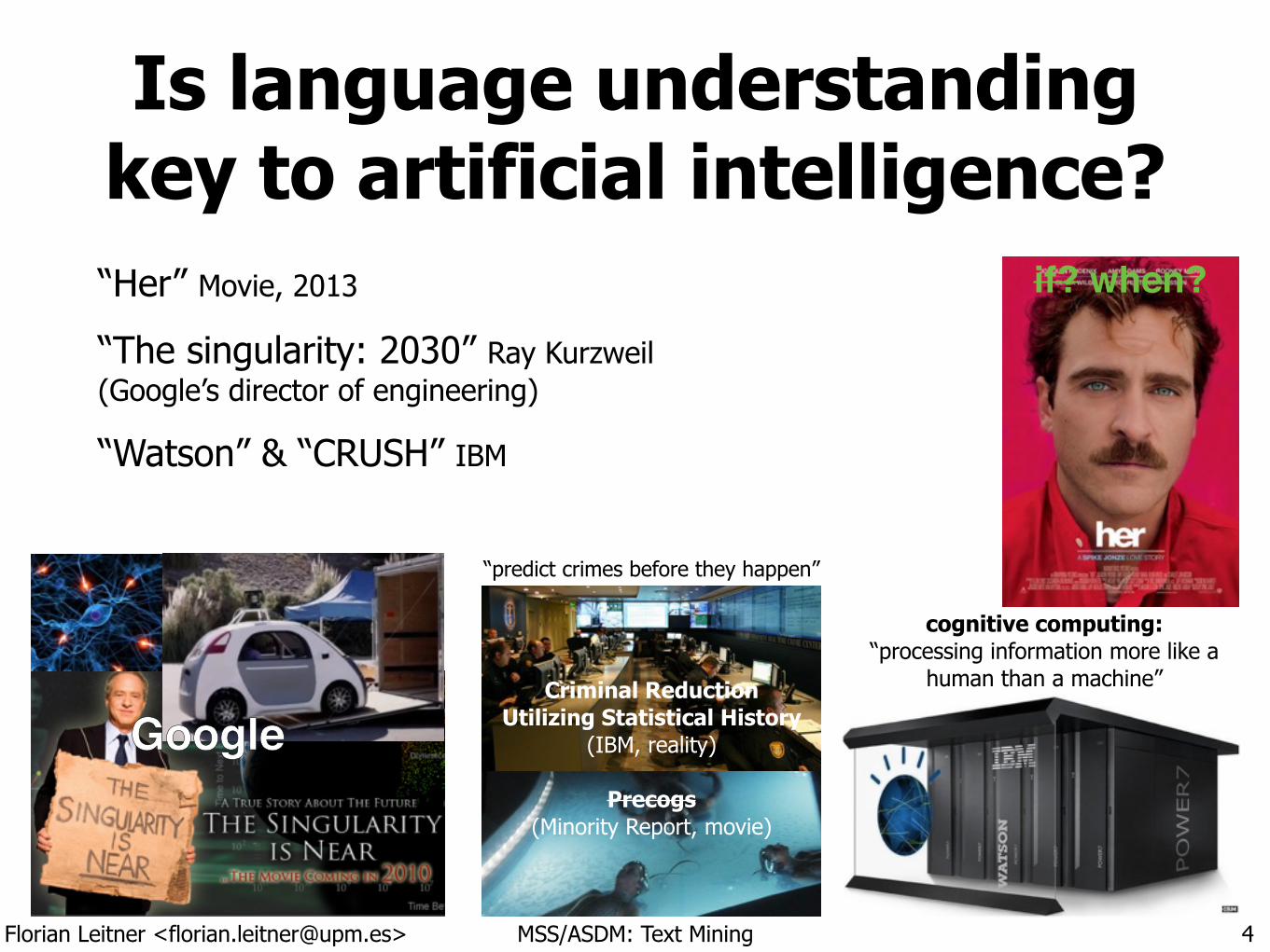
Is language understanding key to artificial intelligence?“Her” Movie, 2013
“The singularity: 2030” Ray Kurzweil(Google’s director of engineering)
“Watson” & “CRUSH” IBM
4
“predict crimes before they happen”
Criminal Reduction Utilizing Statistical History
(IBM, reality) !
Precogs (Minority Report, movie)
if? when?
cognitive computing: “processing information more like a
human than a machine”
GoogleGoogle
Florian Leitner <[email protected]> MSS/ASDM: Text Mining
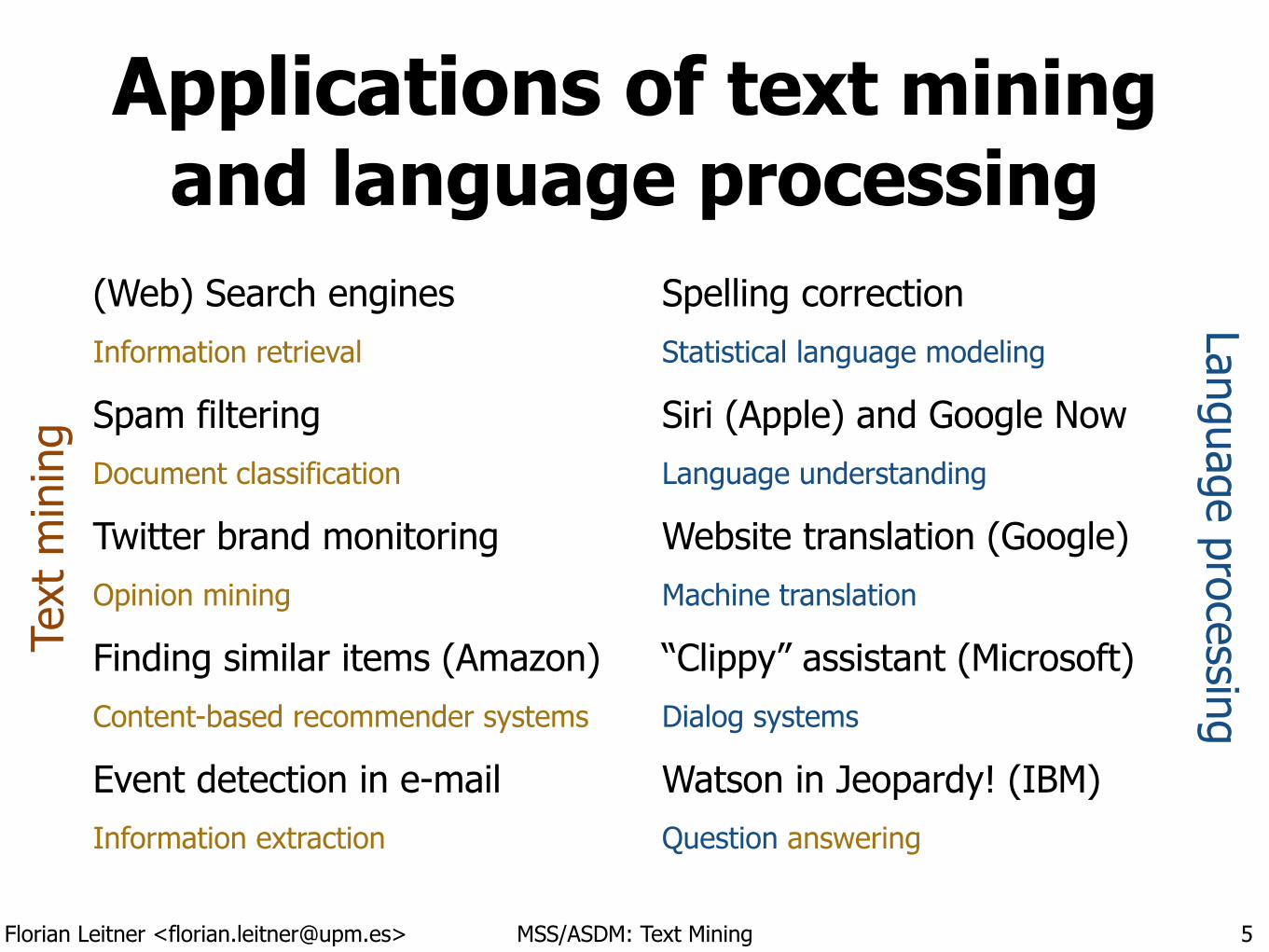
Applications of text mining and language processing
(Web) Search engines Information retrieval
Spam filtering Document classification
Twitter brand monitoring Opinion mining
Finding similar items (Amazon) Content-based recommender systems
Event detection in e-mail Information extraction
Spelling correction Statistical language modeling
Siri (Apple) and Google Now Language understanding
Website translation (Google) Machine translation
“Clippy” assistant (Microsoft) Dialog systems
Watson in Jeopardy! (IBM) Question answering
5
Text
min
ing
Language processing
Florian Leitner <[email protected]> MSS/ASDM: Text Mining
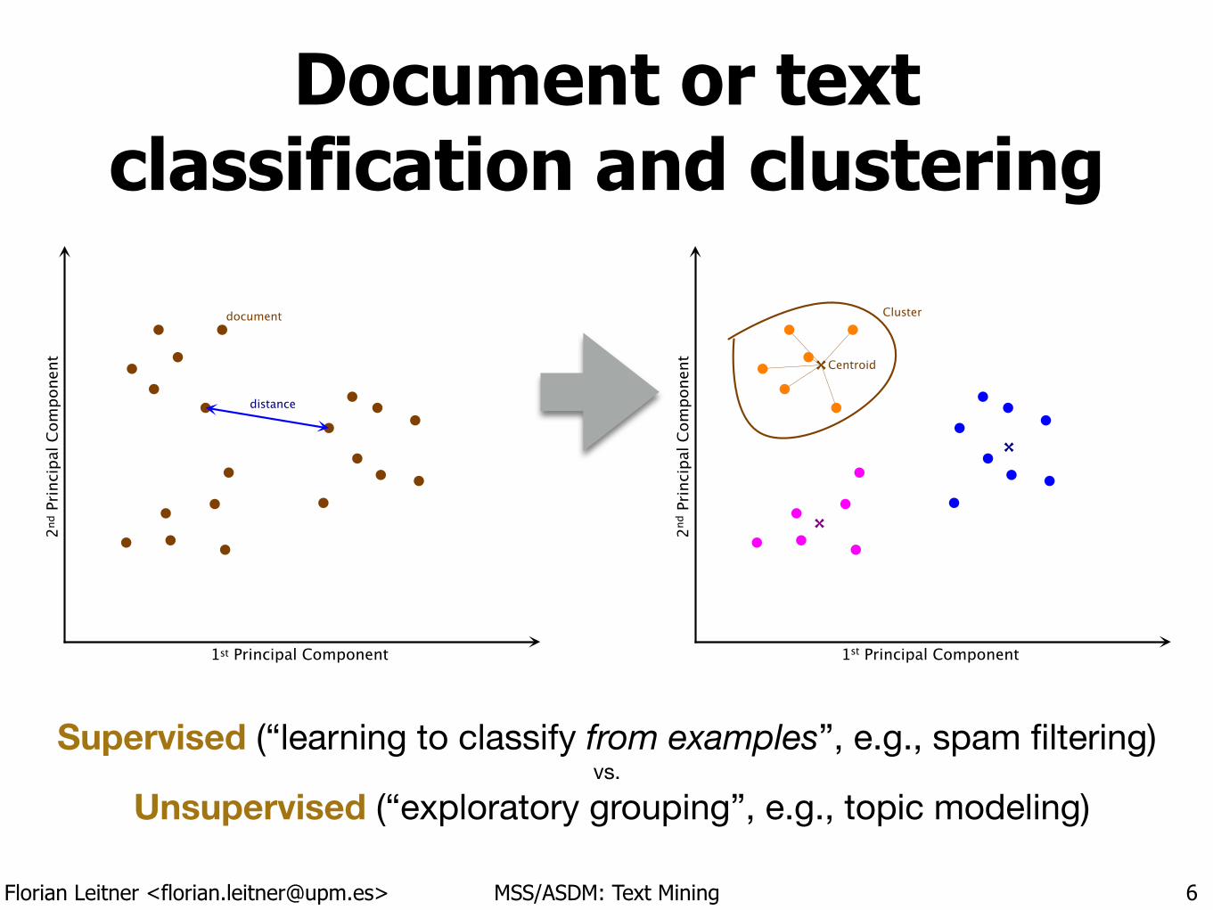
Document or textclassification and clustering
6
1st Principal Component
2nd
Pri
ncip
al C
ompon
ent
document
distance
1st Principal Component
2nd
Pri
ncip
al C
ompon
ent
Centroid
Cluster
Supervised (“learning to classify from examples”, e.g., spam filtering)vs.
Unsupervised (“exploratory grouping”, e.g., topic modeling)
Florian Leitner <[email protected]> MSS/ASDM: Text Mining
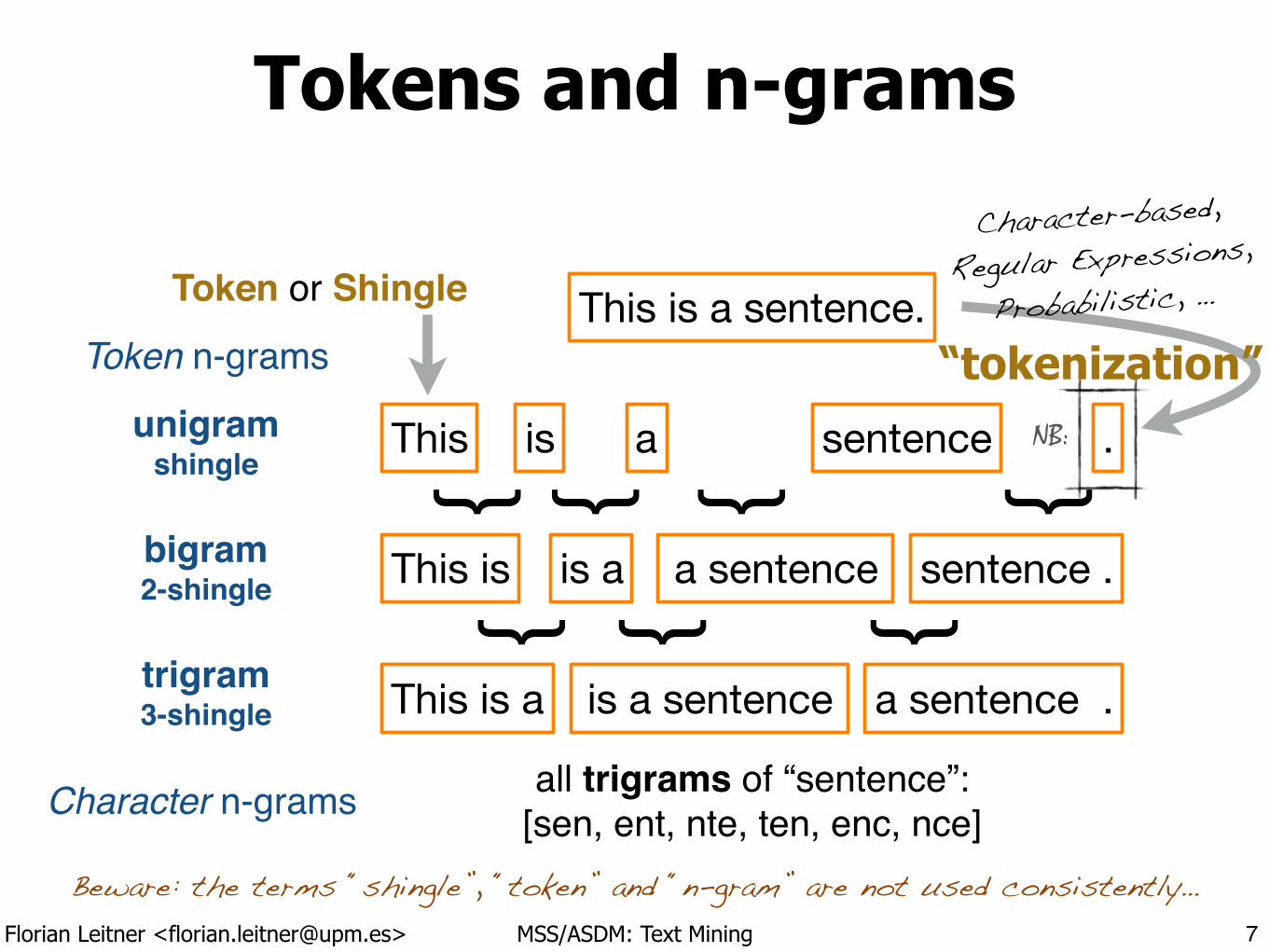
Tokens and n-grams
7
This is a sentence .
This is is a a sentence sentence .
This is a is a sentence a sentence .
This is a sentence.
{ { { {
{ { {
NB:
“tokenization”
Character-based,
Regular Expressions,
Probabilistic, …
Token n-grams
unigram!shingle!
!bigram!2-shingle!
!trigram!3-shingle
all trigrams of “sentence”:[sen, ent, nte, ten, enc, nce]
Beware: the terms “shingle”, “token” and “n-gram” are not used consistently…
Character n-grams
Token or Shingle
Florian Leitner <[email protected]> MSS/ASDM: Text Mining
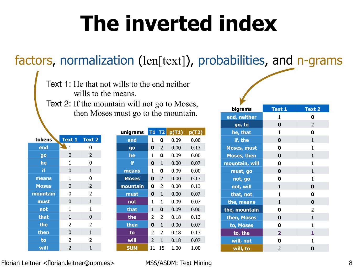
The inverted index
8
Text 1: He that not wills to the end neither wills to the means. Text 2: If the mountain will not go to Moses, then Moses must go to the mountain.
tokens Text 1 Text 2
end 1 0go 0 2
he 1 0
if 0 1
means 1 0
Moses 0 2
mountain 0 2
must 0 1
not 1 1
that 1 0
the 2 2
then 0 1
to 2 2
will 2 1
unigrams T11
T2 p(T1) p(T2)
end 1 0 0.09 0.00go 0 2 0.00 0.13
he 1 0 0.09 0.00
if 0 1 0.00 0.07
means 1 0 0.09 0.00
Moses 0 2 0.00 0.13
mountain 0 2 0.00 0.13
must 0 1 0.00 0.07
not 1 1 0.09 0.07
that 1 0 0.09 0.00
the 2 2 0.18 0.13
then 0 1 0.00 0.07
to 2 2 0.18 0.13
will 2 1 0.18 0.07
SUM 11 15 1.00 1.00
factors, normalization (len[text]), probabilities, and n-grams
bigrams Text 1 Text 2
end, neither 1 0go, to 0 2
he, that 1 0if, the 0 1
Moses, must 0 1
Moses, then 0 1
mountain, will 0 1
must, go 0 1
not, go 0 1
not, will 1 0that, not 1 0
the, means 1 0the, mountain 0 2
then, Moses 0 1
to, Moses 0 1
to, the 2 1will, not 0 1
will, to 2 0
Florian Leitner <[email protected]> MSS/ASDM: Text Mining
Word vectors
9
0 1 2 3 4 5 6 7 8 9 10
10
0
1
2
3
4
5
6
7
8
9
count(Word1)
coun
t(Word 2)
Text
1
Text2α
γ
βSimilarity(T1, T2) := cos(T1, T2)
count(Word 3
)
Comparing word vectors: Cosine similarity
Collections of vectorized texts: Inverted index
Text 1: He that not wills to the end neither wills to the means. Text 2: If the mountain will not go to Moses, then Moses must go to the mountain.
tokens Text 1 Text 2end 1 0go 0 2he 1 0if 0 1
means 1 0Moses 0 2
mountain 0 2must 0 1not 1 1that 1 0the 2 2
then 0 1to 2 2
will 2 1
INDRI
each
tok
en/w
ord
is a
dim
ensi
on!
� w
ord
vect
or �
� w
ord
vect
or �
Florian Leitner <[email protected]> MSS/ASDM: Text Mining
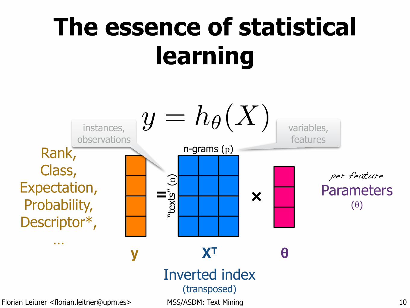
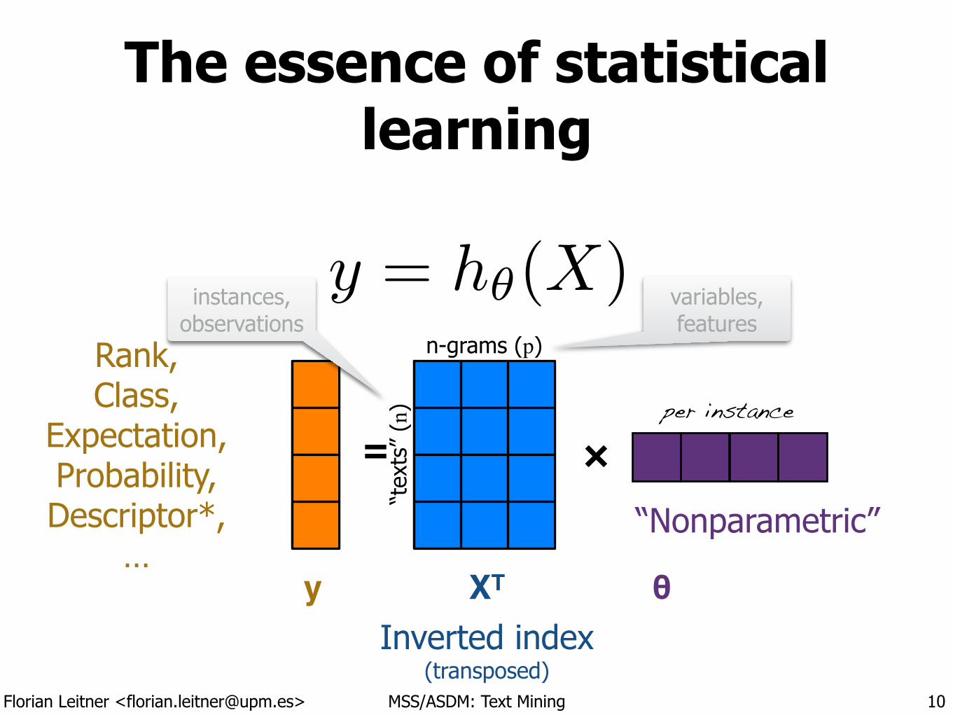
The essence of statistical learning
10
×=
y = h✓(X)
XTy θ
Rank, Class,
Expectation, Probability, Descriptor*,
…
Inverted index (transposed)
Parameters(θ)
“tex
ts”
(n)
n-grams (p)
instances, observations
variables, features
per feature
Florian Leitner <[email protected]> MSS/ASDM: Text Mining
The essence of statistical learning
10
×=
y = h✓(X)
XTy θ
Rank, Class,
Expectation, Probability, Descriptor*,
…
Inverted index (transposed)
Parameters(θ)
“tex
ts”
(n)
n-grams (p)
instances, observations
variables, features
per feature
“Nonparametric”
per instance

Florian Leitner <[email protected]> MSS/ASDM: Text Mining
The curse of dimensionality (RE Bellman, 1961) [inventor of dynamic programming]
• p ≫ n (far more tokens/features thantexts/documents)
• Inverted indices are (discrete) sparse matrices.
• Even with millions of training examples, unseen tokens will keep coming up during evaluation or in production.
• In a high-dimensional hypercube, most instances are closer to the face of the cube (“nothing”, outside) than their nearest neighbor.
11
Florian Leitner <[email protected]> MSS/ASDM: Text Mining
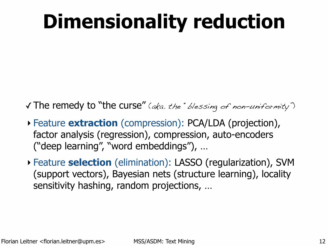
Dimensionality reduction
✓The remedy to “the curse” (aka. the “blessing of non-uniformity”)
‣ Feature extraction (compression): PCA/LDA (projection), factor analysis (regression), compression, auto-encoders (“deep learning”, “word embeddings”), …
‣ Feature selection (elimination): LASSO (regularization), SVM (support vectors), Bayesian nets (structure learning), locality sensitivity hashing, random projections, …
12
Florian Leitner <[email protected]> MSS/ASDM: Text Mining
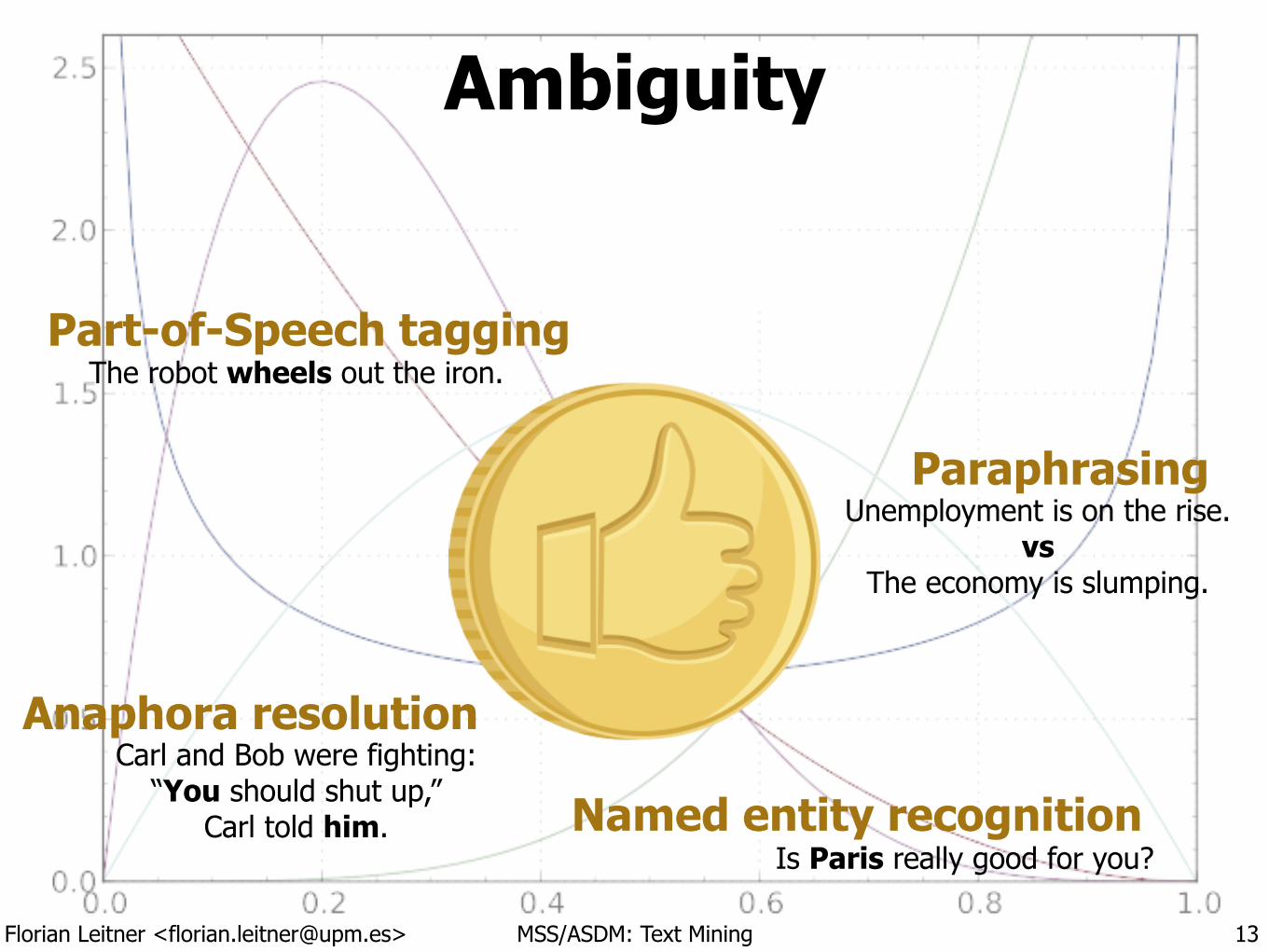
Ambiguity
13
Anaphora resolutionCarl and Bob were fighting:
“You should shut up,” Carl told him.
Part-of-Speech taggingThe robot wheels out the iron.
ParaphrasingUnemployment is on the rise.
vs The economy is slumping.
Named entity recognitionIs Paris really good for you?
Florian Leitner <[email protected]> MSS/ASDM: Text Mining
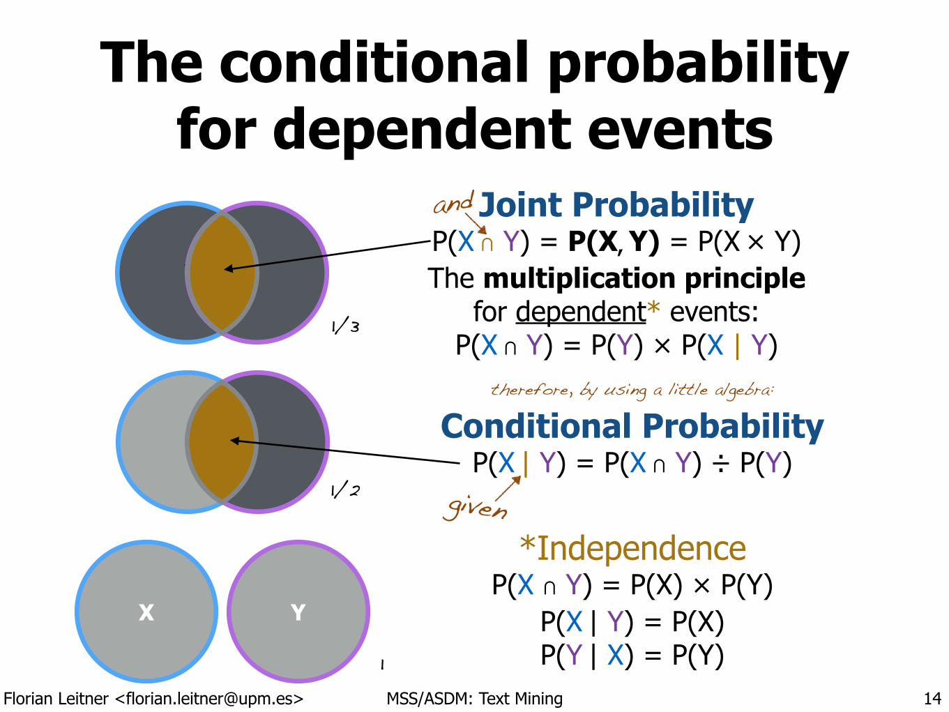
The conditional probability for dependent events
14
Conditional Probability P(X | Y) = P(X ∩ Y) ÷ P(Y)
*Independence P(X ∩ Y) = P(X) × P(Y)
P(X | Y) = P(X) P(Y | X) = P(Y)
` `
Joint Probability P(X ∩ Y) = P(X, Y) = P(X × Y) The multiplication principle
for dependent* events: P(X ∩ Y) = P(Y) × P(X | Y)
and
therefore, by using a little algebra:
X Y
1/3
1/2
1
given
Florian Leitner <[email protected]> MSS/ASDM: Text Mining
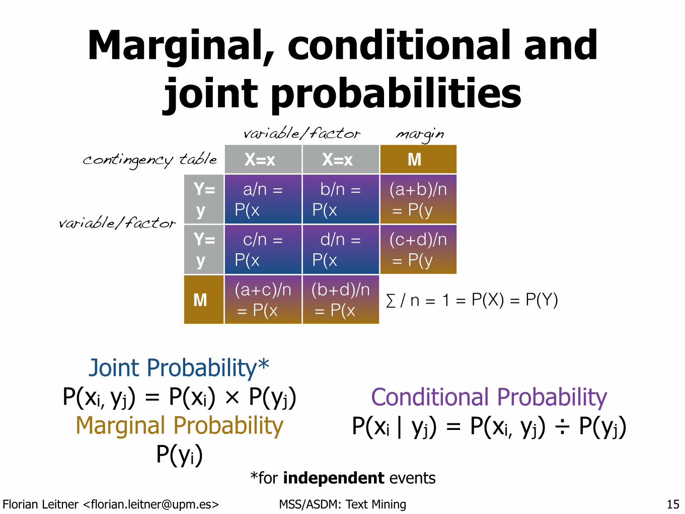
Marginal, conditional and joint probabilities
15
Joint Probability* P(xi, yj) = P(xi) × P(yj) Marginal Probability
P(yi)
X=x X=x MY= y
a/n = P(x
b/n = P(x
(a+b)/n = P(y
Y= y
c/n = P(x
d/n = P(x
(c+d)/n = P(y
M (a+c)/n = P(x
(b+d)/n = P(x ∑ / n = 1 = P(X) = P(Y)
Conditional Probability P(xi | yj) = P(xi, yj) ÷ P(yj)
contingency table
*for independent events
variable/factor
variable/factor margin
Florian Leitner <[email protected]> MSS/ASDM: Text Mining
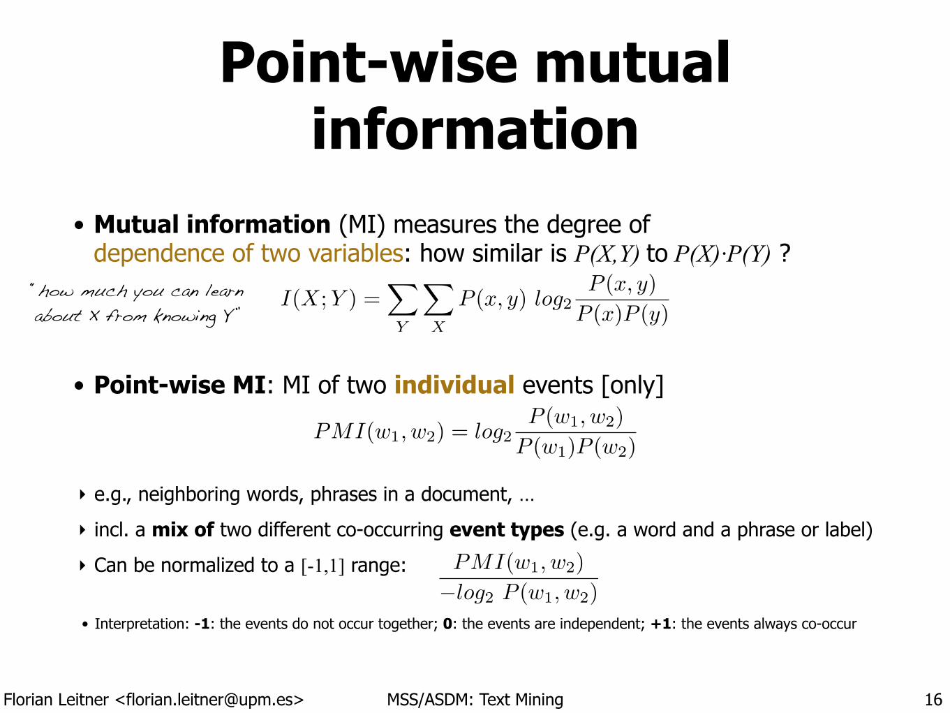
Point-wise mutual information
• Mutual information (MI) measures the degree of dependence of two variables: how similar is P(X,Y) to P(X)·P(Y) ?
!
!
• Point-wise MI: MI of two individual events [only] !!
‣ e.g., neighboring words, phrases in a document, …
‣ incl. a mix of two different co-occurring event types (e.g. a word and a phrase or label)
‣ Can be normalized to a [-1,1] range: !
• Interpretation: -1: the events do not occur together; 0: the events are independent; +1: the events always co-occur
16
I(X;Y ) =X
Y
X
X
P (x, y) log2P (x, y)
P (x)P (y)
PMI(w1, w2) = log2P (w1, w2)
P (w1)P (w2)
PMI(w1, w2)
�log2 P (w1, w2)
“how much you can learn about X from knowing Y”
Florian Leitner <[email protected]> MSS/ASDM: Text Mining
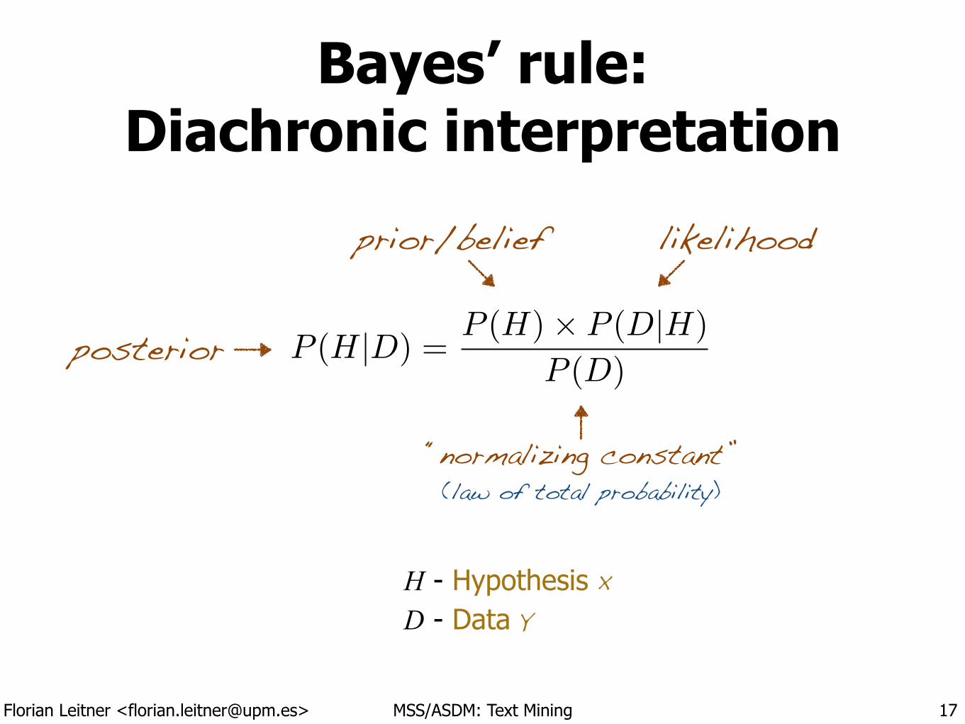
Bayes’ rule: Diachronic interpretation
17
H - Hypothesis X D - Data Y
prior/belief likelihood
posterior P (H|D) =P (H)⇥ P (D|H)
P (D)
“normalizing constant” (law of total probability)
Florian Leitner <[email protected]> MSS/ASDM: Text Mining
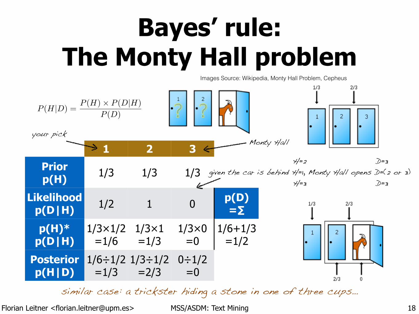
Bayes’ rule: The Monty Hall problem
18
1 2 3
Prior p(H) 1/3 1/3 1/3
Likelihood p(D|H) 1/2 1 0 p(D)
=∑
p(H)* p(D|H)
1/3×1/2 =1/6
1/3×1 =1/3
1/3×0 =0
1/6+1/3 =1/2
Posterior p(H|D)
1/6÷1/2 =1/3
1/3÷1/2 =2/3
0÷1/2 =0
P (H|D) =P (H)⇥ P (D|H)
P (D)
similar case: a trickster hiding a stone in one of three cups…
Images Source: Wikipedia, Monty Hall Problem, Cepheus
your pick
given the car is behind H=1, Monty Hall opens D=(2 or 3)H=2 !
H=3
D=3 !
D=3
Monty Hall
Florian Leitner <[email protected]> MSS/ASDM: Text Mining
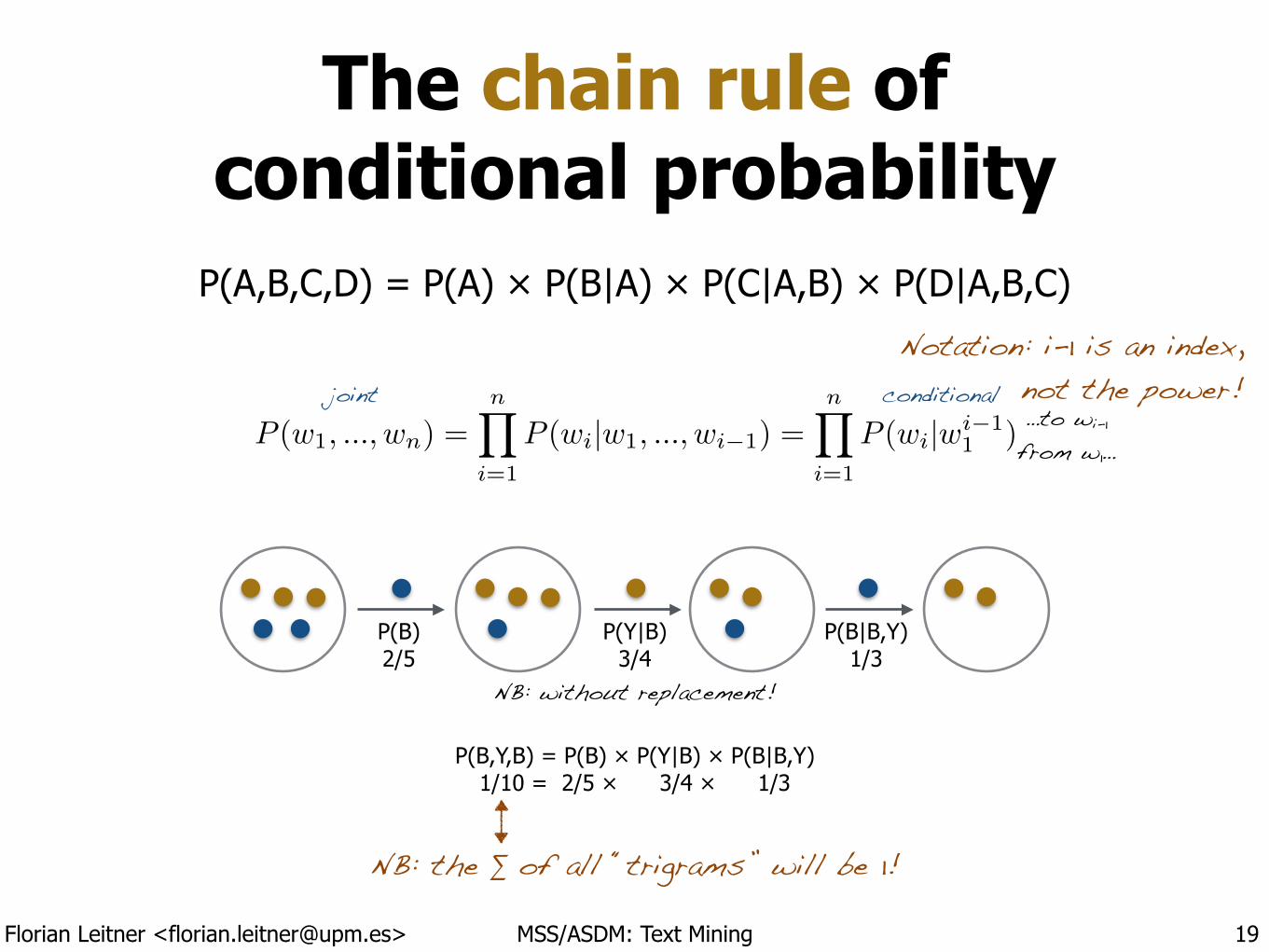
The chain rule of conditional probability
P(A,B,C,D) = P(A) × P(B|A) × P(C|A,B) × P(D|A,B,C)
19
P(B,Y,B) = P(B) × P(Y|B) × P(B|B,Y) 1/10 = 2/5 × 3/4 × 1/3
P(B) 2/5
P(Y|B) 3/4
P(B|B,Y) 1/3
P (w1, ..., wn) =nY
i=1
P (wi|w1, ..., wi�1) =nY
i=1
P (wi|wi�11 )
NB: the ∑ of all “trigrams” will be 1!
NB: without replacement!
joint conditional…to wi-1 from w1…
Notation: i-1 is an index, not the power!
Florian Leitner <[email protected]> MSS/ASDM: Text Mining
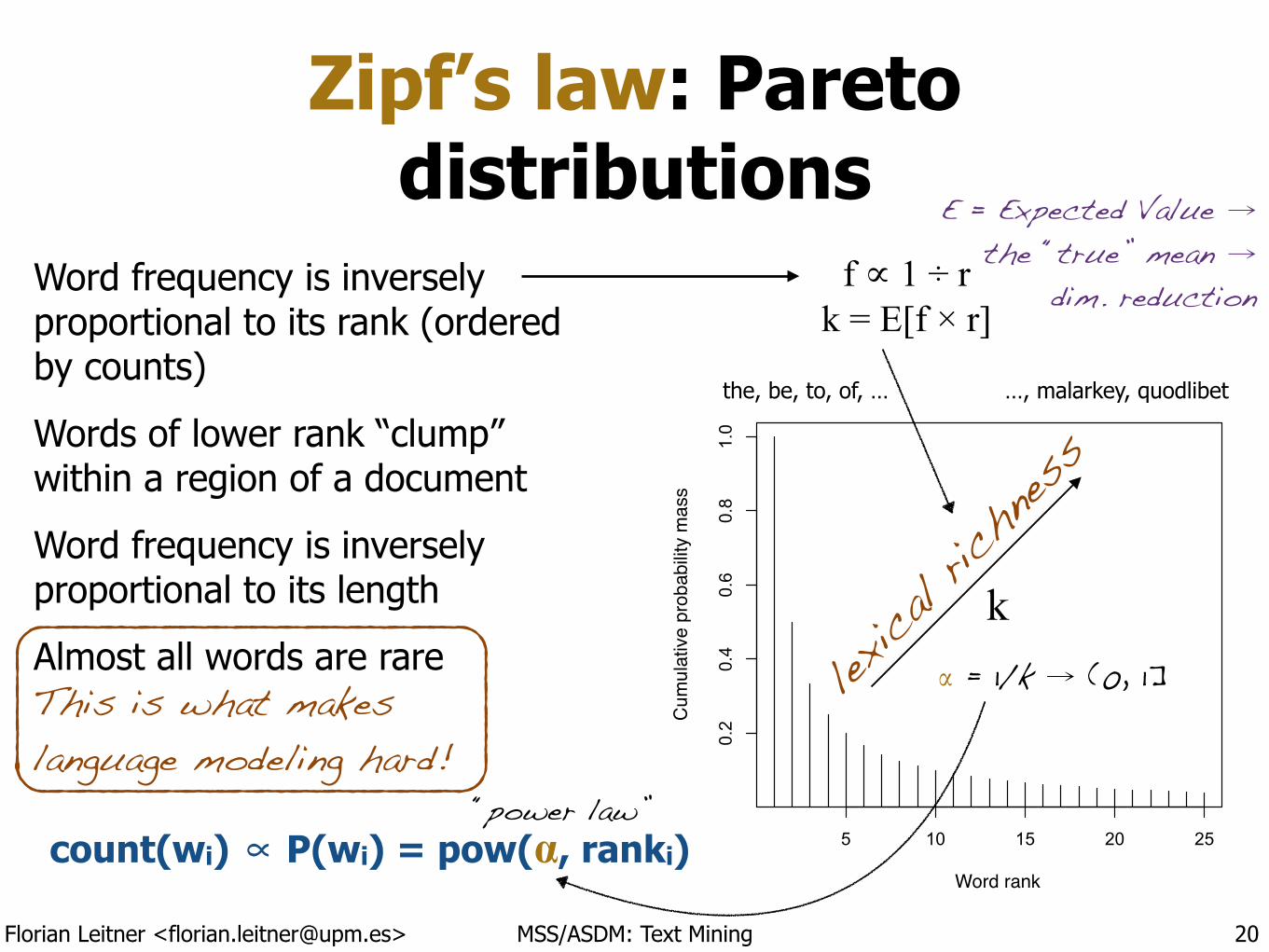
Zipf’s law: Pareto distributions
Word frequency is inversely proportional to its rank (ordered by counts)
Words of lower rank “clump” within a region of a document
Word frequency is inversely proportional to its length
Almost all words are rare
20
f ∝ 1 ÷ r k = E[f × r]
5 10 15 20 25
0.2
0.4
0.6
0.8
1.0
Word
Frequency
lexica
l rich
ness
k
Word rank
This is what makes language modeling hard!
the, be, to, of, … …, malarkey, quodlibet
E = Expected Value � the “true” mean �
dim. reduction
Cum
ulat
ive
prob
abilit
y m
ass
count(wi) ∝ P(wi) = pow(α, ranki)
� = 1/k � (0, 1]
“power law”
Florian Leitner <[email protected]> MSS/ASDM: Text Mining
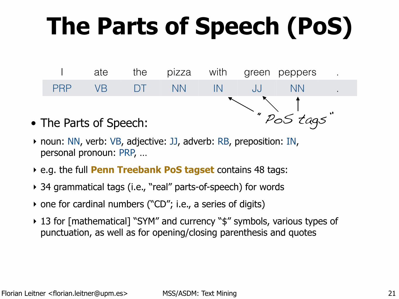
The Parts of Speech (PoS)
• The Parts of Speech: ‣ noun: NN, verb: VB, adjective: JJ, adverb: RB, preposition: IN,
personal pronoun: PRP, …
‣ e.g. the full Penn Treebank PoS tagset contains 48 tags:
‣ 34 grammatical tags (i.e., “real” parts-of-speech) for words
‣ one for cardinal numbers (“CD”; i.e., a series of digits)
‣ 13 for [mathematical] “SYM” and currency “$” symbols, various types of punctuation, as well as for opening/closing parenthesis and quotes
21
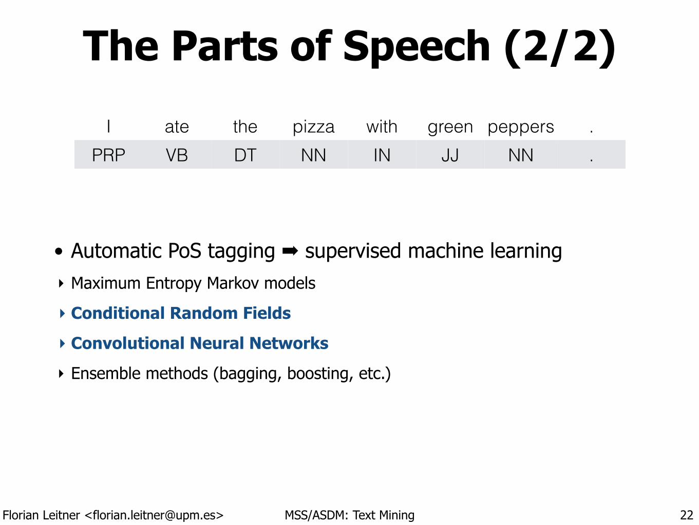
I ate the pizza with green peppers .PRP VB DT NN IN JJ NN .
“PoS tags”
Florian Leitner <[email protected]> MSS/ASDM: Text Mining
The Parts of Speech (2/2)
• Automatic PoS tagging ➡ supervised machine learning ‣ Maximum Entropy Markov models
‣ Conditional Random Fields
‣ Convolutional Neural Networks
‣ Ensemble methods (bagging, boosting, etc.)
22
I ate the pizza with green peppers .PRP VB DT NN IN JJ NN .
Florian Leitner <[email protected]> MSS/ASDM: Text Mining
Linguistic morphology
• [Verbal] Inflections ‣ conjugation (Indo-European
languages)
‣ tense (“availability” and use varies across languages)
‣ modality (subjunctive, conditional, imperative)
‣ voice (active/passive)
‣ …
!
• Contractions ‣ don’t say you’re in a man’s world…
• Declensions • on nouns, pronouns, adjectives, determiners
‣ case (nominative, accusative, dative, ablative, genitive, …)
‣ gender (female, male, neuter)
‣ number forms (singular, plural, dual)
‣ possessive pronouns (I➞my, you➞your, she➞her, it➞its, … car)
‣ reflexive pronouns (for myself, yourself, …)
‣ …
23
not a contraction: possessive s
➡ token normalization
Florian Leitner <[email protected]> MSS/ASDM: Text Mining
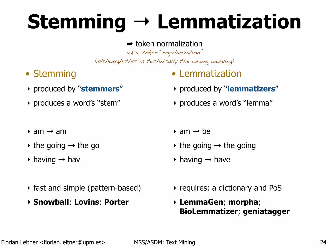
Stemming → Lemmatization
• Stemming ‣ produced by “stemmers”
‣ produces a word’s “stem”
!
‣ am ➞ am
‣ the going ➞ the go
‣ having ➞ hav
!
‣ fast and simple (pattern-based)
‣ Snowball; Lovins; Porter
!
• Lemmatization ‣ produced by “lemmatizers”
‣ produces a word’s “lemma”
!
‣ am ➞ be
‣ the going ➞ the going
‣ having ➞ have
!
‣ requires: a dictionary and PoS
‣ LemmaGen; morpha; BioLemmatizer; geniatagger
24
➡ token normalizationa.k.a. token “regularization”
(although that is technically the wrong wording)
Florian Leitner <[email protected]> MSS/ASDM: Text Mining
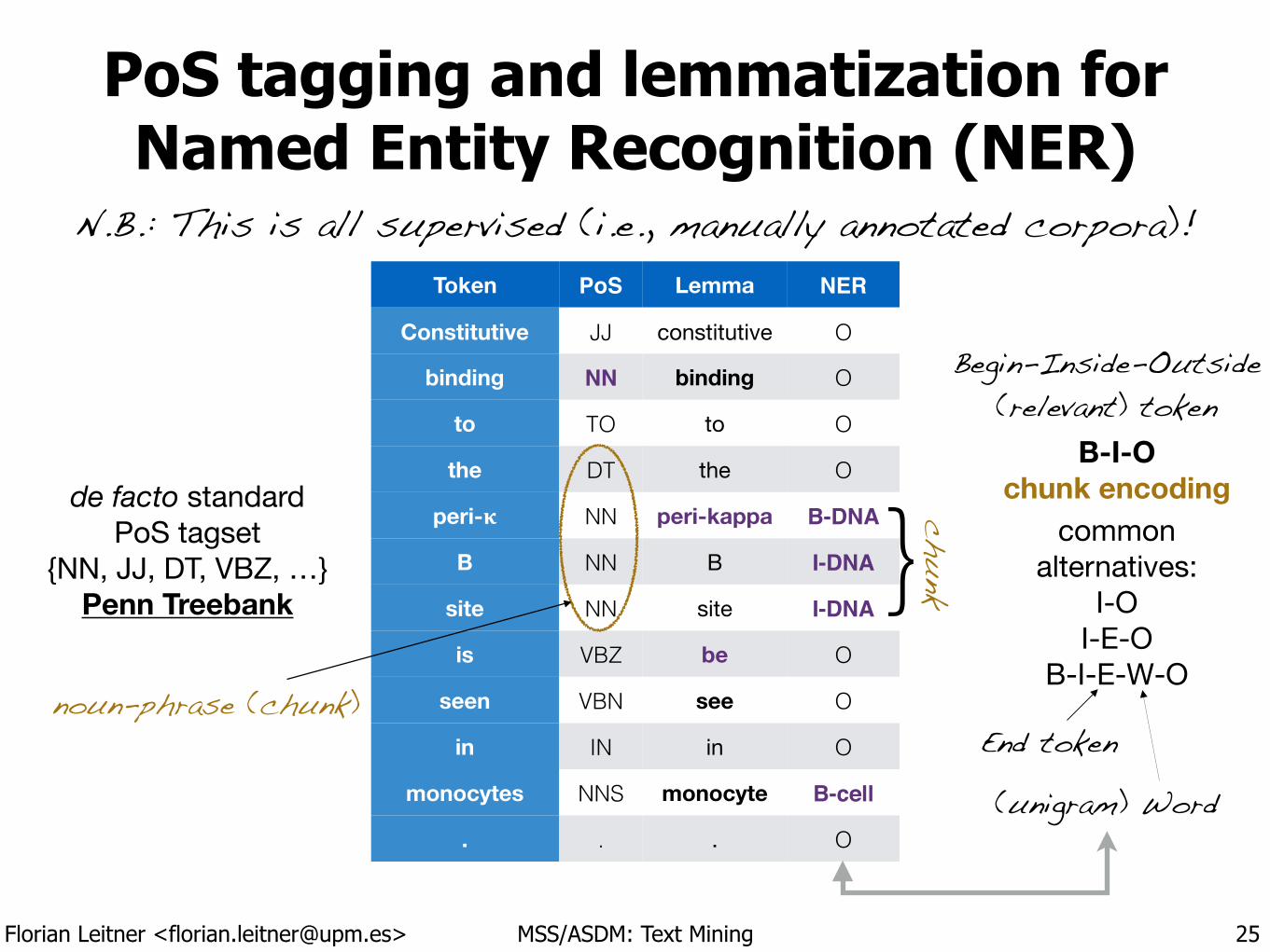
PoS tagging and lemmatization forNamed Entity Recognition (NER)
25
Token PoS Lemma NER
Constitutive JJ constitutive O
binding NN binding O
to TO to O
the DT the O
peri-! NN peri-kappa B-DNA
B NN B I-DNA
site NN site I-DNA
is VBZ be O
seen VBN see O
in IN in O
monocytes NNS monocyte B-cell
. . . O
de facto standard PoS tagset
{NN, JJ, DT, VBZ, …}Penn Treebank
B-I-O chunk encoding
commonalternatives:
I-OI-E-O
B-I-E-W-O
End token
(unigram) Word
Begin-Inside-Outside (relevant) token
} chunk
noun-phrase (chunk)
N.B.: This is all supervised (i.e., manually annotated corpora)!
Florian Leitner <[email protected]> MSS/ASDM: Text Mining
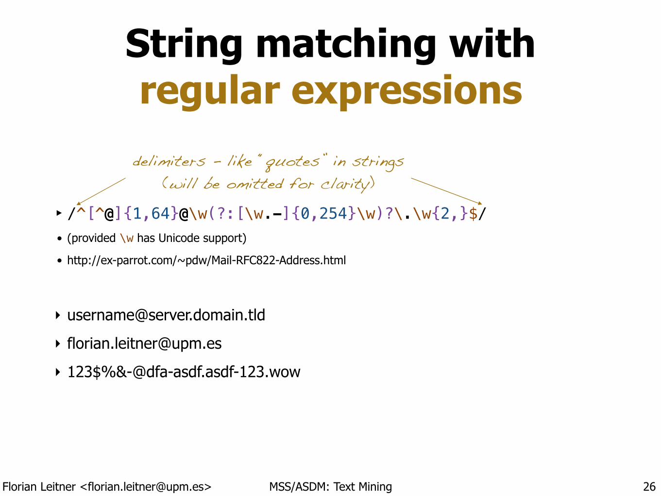
String matching with regular expressions
‣ /^[^@]{1,64}@\w(?:[\w.-]{0,254}\w)?\.\w{2,}$/ • (provided \w has Unicode support)
• http://ex-parrot.com/~pdw/Mail-RFC822-Address.html
!
‣ 123$%&[email protected]
26
delimiters - like “quotes” in strings (will be omitted for clarity)
Florian Leitner <[email protected]> MSS/ASDM: Text Mining
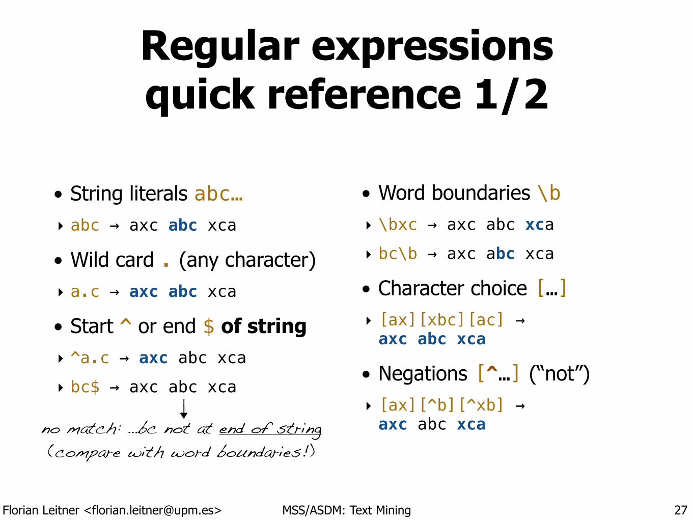
Regular expressionsquick reference 1/2
• String literals abc… ‣ abc → axc abc xca
• Wild card . (any character) ‣ a.c → axc abc xca
• Start ^ or end $ of string ‣ ^a.c → axc abc xca ‣ bc$ → axc abc xca
!
• Word boundaries \b ‣ \bxc → axc abc xca ‣ bc\b → axc abc xca
• Character choice […] ‣ [ax][xbc][ac] → axc abc xca
• Negations [^…] (“not”) ‣ [ax][^b][^xb] → axc abc xca
27
no match: …bc not at end of string (compare with word boundaries!)
Florian Leitner <[email protected]> MSS/ASDM: Text Mining
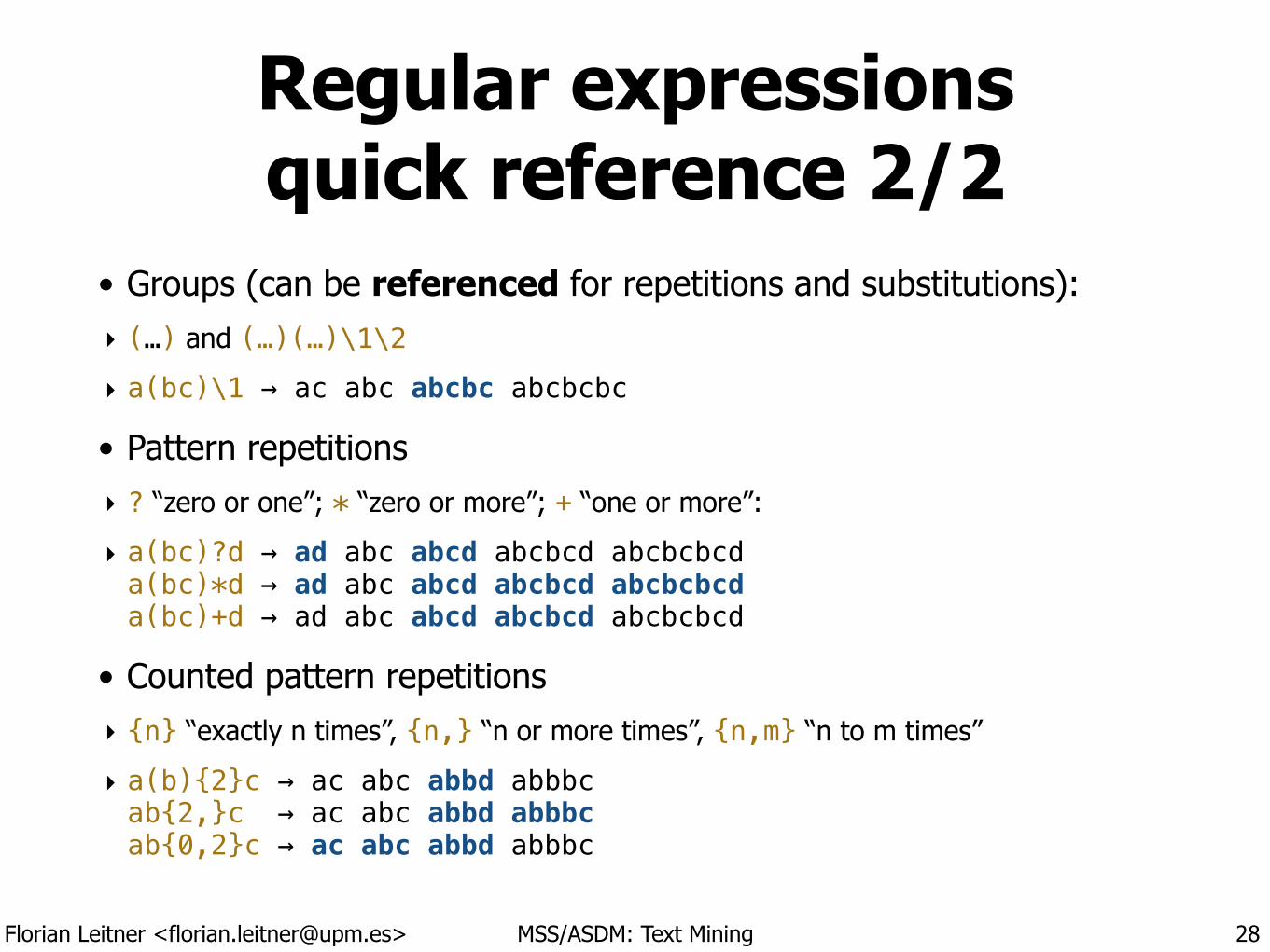
Regular expressions quick reference 2/2
• Groups (can be referenced for repetitions and substitutions): ‣ (…) and (…)(…)\1\2
‣ a(bc)\1 → ac abc abcbc abcbcbc
• Pattern repetitions ‣ ? “zero or one”; * “zero or more”; + “one or more”:
‣ a(bc)?d → ad abc abcd abcbcd abcbcbcda(bc)*d → ad abc abcd abcbcd abcbcbcda(bc)+d → ad abc abcd abcbcd abcbcbcd
• Counted pattern repetitions ‣ {n} “exactly n times”, {n,} “n or more times”, {n,m} “n to m times”
‣ a(b){2}c → ac abc abbd abbbcab{2,}c → ac abc abbd abbbcab{0,2}c → ac abc abbd abbbc
28
Florian Leitner <[email protected]> MSS/ASDM: Text Mining
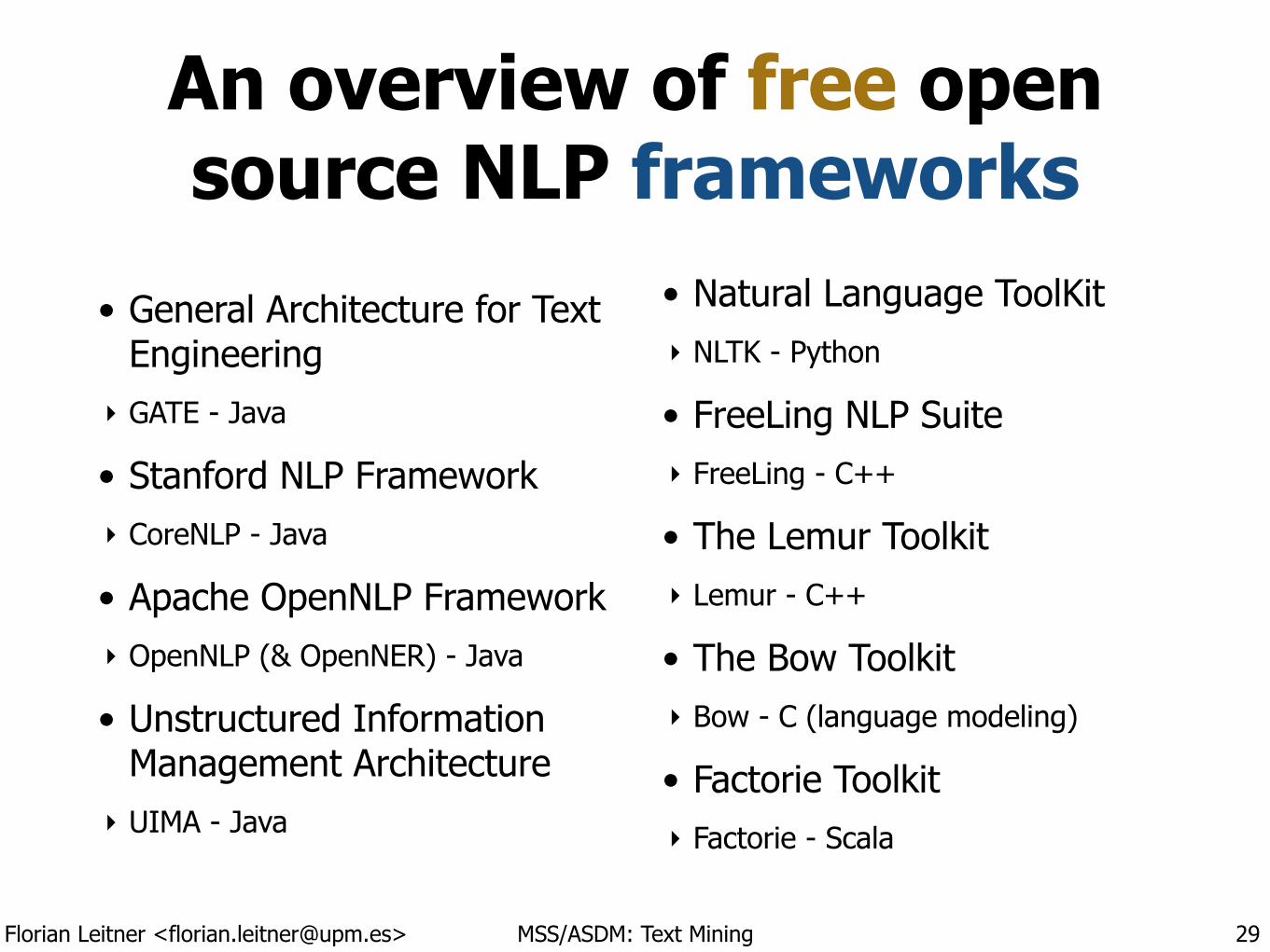
An overview of free open source NLP frameworks
• General Architecture for Text Engineering
‣ GATE - Java
• Stanford NLP Framework ‣ CoreNLP - Java
• Apache OpenNLP Framework ‣ OpenNLP (& OpenNER) - Java
• Unstructured Information Management Architecture
‣ UIMA - Java
• Natural Language ToolKit ‣ NLTK - Python
• FreeLing NLP Suite ‣ FreeLing - C++
• The Lemur Toolkit ‣ Lemur - C++
• The Bow Toolkit ‣ Bow - C (language modeling)
• Factorie Toolkit ‣ Factorie - Scala
29
Florian Leitner <[email protected]> MSS/ASDM: Text Mining
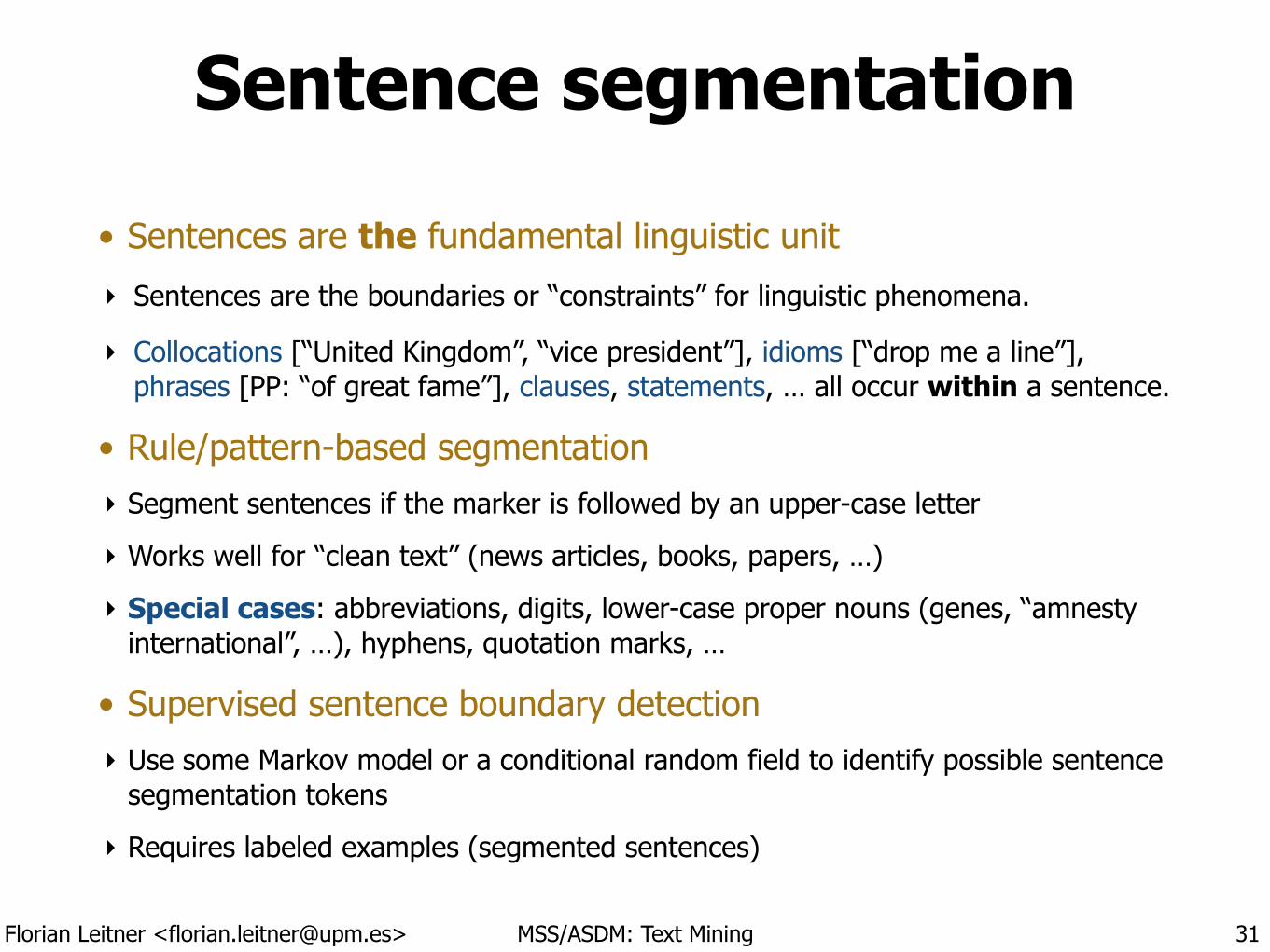
Sentence segmentation
• Sentences are the fundamental linguistic unit
‣ Sentences are the boundaries or “constraints” for linguistic phenomena.
‣ Collocations [“United Kingdom”, “vice president”], idioms [“drop me a line”], phrases [PP: “of great fame”], clauses, statements, … all occur within a sentence.
• Rule/pattern-based segmentation ‣ Segment sentences if the marker is followed by an upper-case letter
‣ Works well for “clean text” (news articles, books, papers, …)
‣ Special cases: abbreviations, digits, lower-case proper nouns (genes, “amnesty international”, …), hyphens, quotation marks, …
• Supervised sentence boundary detection ‣ Use some Markov model or a conditional random field to identify possible sentence
segmentation tokens
‣ Requires labeled examples (segmented sentences)
31
Florian Leitner <[email protected]> MSS/ASDM: Text Mining
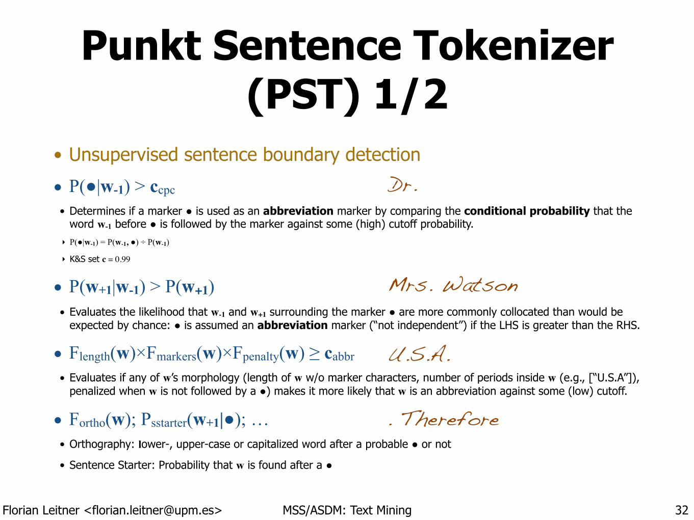
Punkt Sentence Tokenizer (PST) 1/2
• Unsupervised sentence boundary detection
• P(●|w-1) > ccpc • Determines if a marker ● is used as an abbreviation marker by comparing the conditional probability that the
word w-1 before ● is followed by the marker against some (high) cutoff probability. ‣ P(●|w-1) = P(w-1, ●) ÷ P(w-1)
‣ K&S set c = 0.99
• P(w+1|w-1) > P(w+1) • Evaluates the likelihood that w-1 and w+1 surrounding the marker ● are more commonly collocated than would be
expected by chance: ● is assumed an abbreviation marker (“not independent”) if the LHS is greater than the RHS.
• Flength(w)×Fmarkers(w)×Fpenalty(w) ≥ cabbr • Evaluates if any of w’s morphology (length of w w/o marker characters, number of periods inside w (e.g., [“U.S.A”]),
penalized when w is not followed by a ●) makes it more likely that w is an abbreviation against some (low) cutoff.
• Fortho(w); Psstarter(w+1|●); … • Orthography: lower-, upper-case or capitalized word after a probable ● or not
• Sentence Starter: Probability that w is found after a ●
32
Dr.
Mrs. Watson
U.S.A.
. Therefore
Florian Leitner <[email protected]> MSS/ASDM: Text Mining
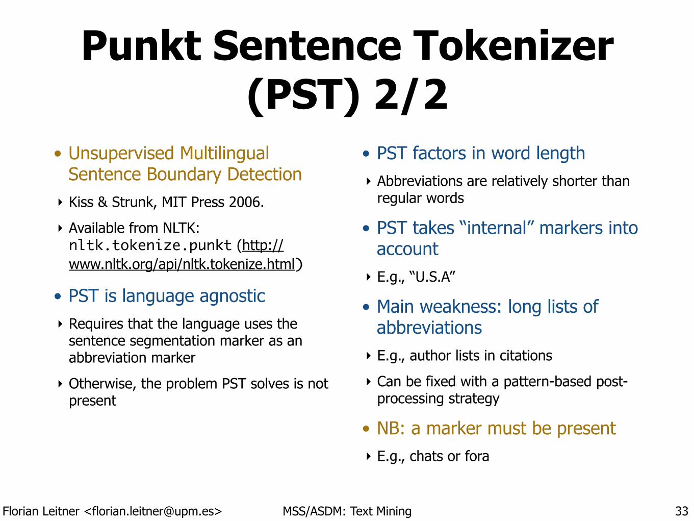
Punkt Sentence Tokenizer (PST) 2/2
• Unsupervised Multilingual Sentence Boundary Detection
‣ Kiss & Strunk, MIT Press 2006.
‣ Available from NLTK: nltk.tokenize.punkt (http://www.nltk.org/api/nltk.tokenize.html)
• PST is language agnostic ‣ Requires that the language uses the
sentence segmentation marker as an abbreviation marker
‣ Otherwise, the problem PST solves is not present
!!
• PST factors in word length ‣ Abbreviations are relatively shorter than
regular words
• PST takes “internal” markers into account
‣ E.g., “U.S.A”
• Main weakness: long lists of abbreviations
‣ E.g., author lists in citations
‣ Can be fixed with a pattern-based post-processing strategy
• NB: a marker must be present ‣ E.g., chats or fora
33
Text Mining 2 Language Modeling
!Madrid Summer School on
Advanced Statistics and Data Mining !
Florian Leitner [email protected]
License:
Florian Leitner <[email protected]> MSS/ASDM: Text Mining
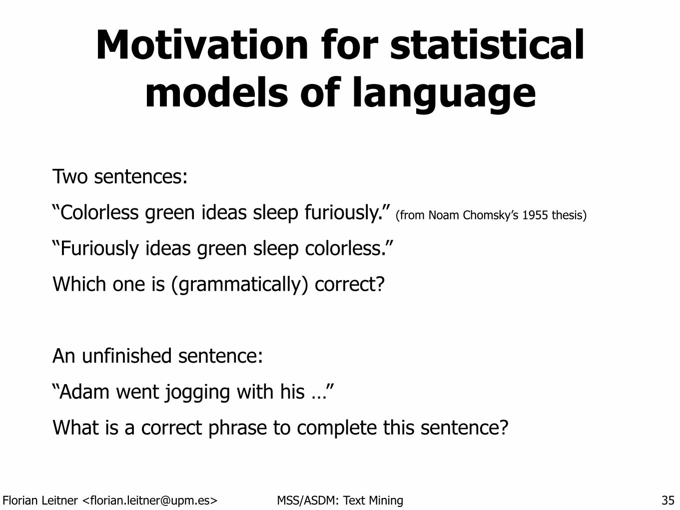
Motivation for statistical models of language
Two sentences:
“Colorless green ideas sleep furiously.” (from Noam Chomsky’s 1955 thesis)
“Furiously ideas green sleep colorless.”
Which one is (grammatically) correct?
!
An unfinished sentence:
“Adam went jogging with his …”
What is a correct phrase to complete this sentence?
35
Florian Leitner <[email protected]> MSS/ASDM: Text Mining
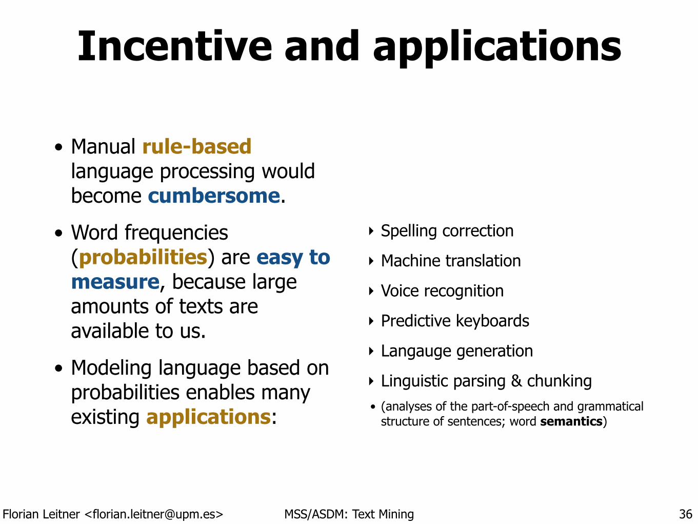
Incentive and applications!
• Manual rule-based language processing would become cumbersome.
• Word frequencies (probabilities) are easy to measure, because large amounts of texts are available to us.
• Modeling language based on probabilities enables many existing applications:
‣ Spelling correction
‣ Machine translation
‣ Voice recognition
‣ Predictive keyboards
‣ Langauge generation
‣ Linguistic parsing & chunking • (analyses of the part-of-speech and grammatical
structure of sentences; word semantics)
36
Florian Leitner <[email protected]> MSS/ASDM: Text Mining
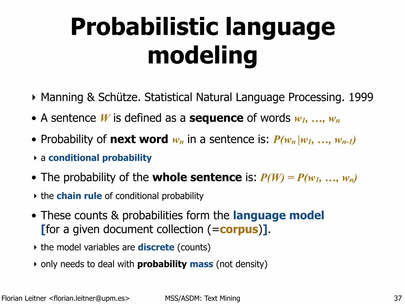
Probabilistic language modeling
‣ Manning & Schütze. Statistical Natural Language Processing. 1999
• A sentence W is defined as a sequence of words w1, …, wn
• Probability of next word wn in a sentence is: P(wn |w1, …, wn-1) ‣ a conditional probability
• The probability of the whole sentence is: P(W) = P(w1, …, wn) ‣ the chain rule of conditional probability
• These counts & probabilities form the language model[for a given document collection (=corpus)].
‣ the model variables are discrete (counts)
‣ only needs to deal with probability mass (not density)
37
Florian Leitner <[email protected]> MSS/ASDM: Text Mining
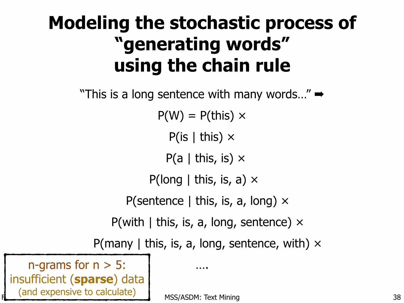
Modeling the stochastic process of “generating words” using the chain rule
“This is a long sentence with many words…” ➡
P(W) = P(this) ×
P(is | this) ×
P(a | this, is) ×
P(long | this, is, a) ×
P(sentence | this, is, a, long) ×
P(with | this, is, a, long, sentence) ×
P(many | this, is, a, long, sentence, with) ×
….
38
n-grams for n > 5: insufficient (sparse) data
(and expensive to calculate)
Florian Leitner <[email protected]> MSS/ASDM: Text Mining
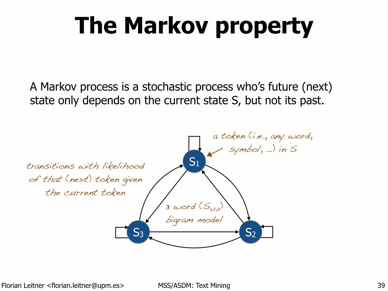
The Markov property
A Markov process is a stochastic process who’s future (next) state only depends on the current state S, but not its past.
39
S1
S2S3
a token (i.e., any word, symbol, …) in S
transitions with likelihood of that (next) token given
the current token3 word (S1,2,3) bigram model
Florian Leitner <[email protected]> MSS/ASDM: Text Mining
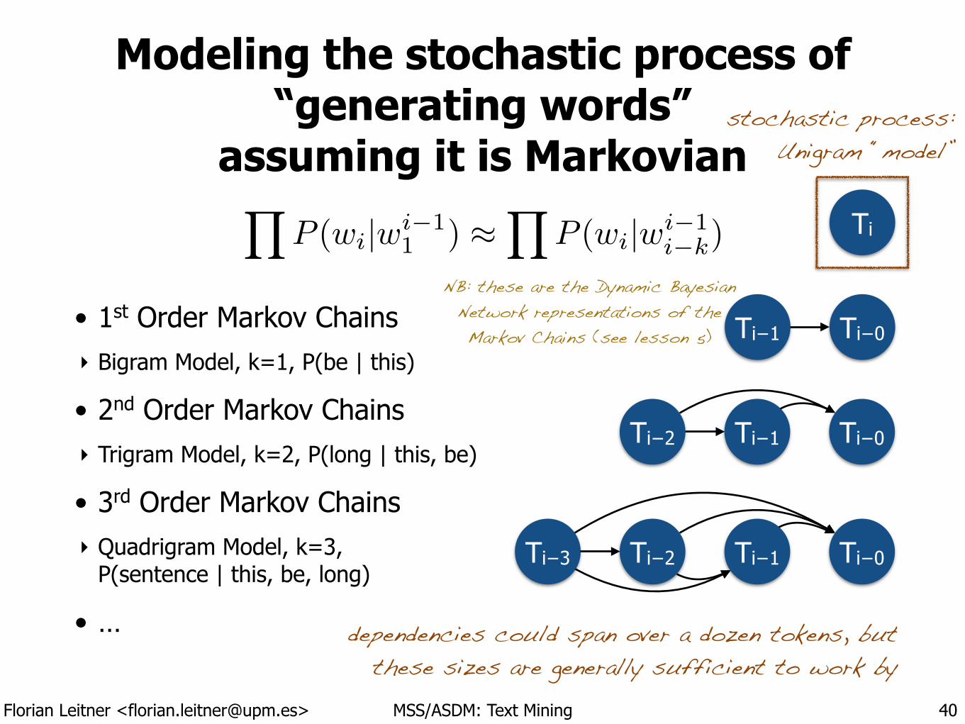
Modeling the stochastic process of “generating words”
assuming it is Markovian!
!
• 1st Order Markov Chains ‣ Bigram Model, k=1, P(be | this)
• 2nd Order Markov Chains ‣ Trigram Model, k=2, P(long | this, be)
• 3rd Order Markov Chains ‣ Quadrigram Model, k=3,
P(sentence | this, be, long)
• …
40
Ti−0Ti−1
Ti−0Ti−1Ti−2Ti−3
Ti−0Ti−1Ti−2
dependencies could span over a dozen tokens, but these sizes are generally sufficient to work by
YP (wi|wi�1
1 ) ⇡Y
P (wi|wi�1i�k)
Ti
stochastic process: Unigram “model”
NB: these are the Dynamic Bayesian Network representations of the Markov Chains (see lesson 5)
Florian Leitner <[email protected]> MSS/ASDM: Text Mining
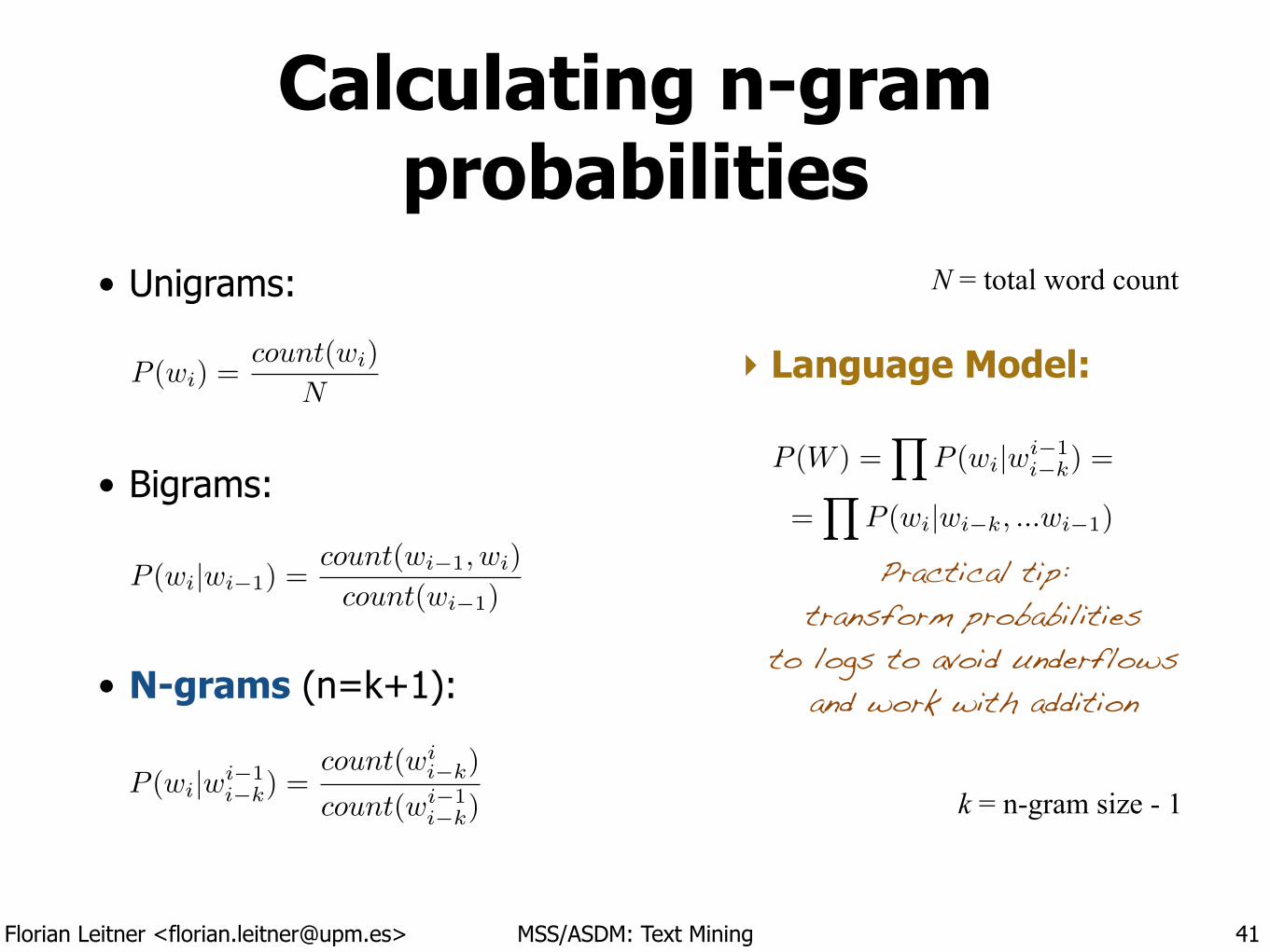
• Unigrams:
• Bigrams:
• N-grams (n=k+1):
Calculating n-gram probabilities
41
P (wi|wi�1) =count(wi�1, wi)
count(wi�1)
P (wi) =count(wi)
N
N = total word count
P (wi|wi�1i�k) =
count(wii�k)
count(wi�1i�k) k = n-gram size - 1
‣ Language Model:
Practical tip: transform probabilities
to logs to avoid underflows and work with addition
P (W ) =Y
P (wi|wi�1i�k) =
=Y
P (wi|wi�k, ...wi�1)
Florian Leitner <[email protected]> MSS/ASDM: Text Mining
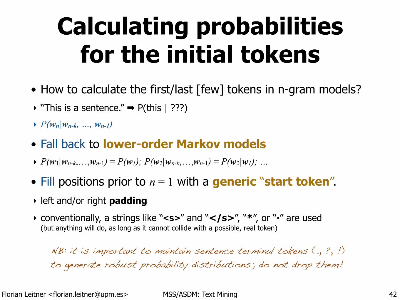
Calculating probabilities for the initial tokens
• How to calculate the first/last [few] tokens in n-gram models? ‣ “This is a sentence.” ➡ P(this | ???)
‣ P(wn|wn-k, …, wn-1)
• Fall back to lower-order Markov models ‣ P(w1|wn-k,…,wn-1) = P(w1); P(w2|wn-k,…,wn-1) = P(w2|w1); …
• Fill positions prior to n = 1 with a generic “start token”. ‣ left and/or right padding
‣ conventionally, a strings like “<s>” and “</s>”, “*”, or “·” are used (but anything will do, as long as it cannot collide with a possible, real token)
42
NB: it is important to maintain sentence terminal tokens (., ?, !) to generate robust probability distributions; do not drop them!
Florian Leitner <[email protected]> MSS/ASDM: Text Mining
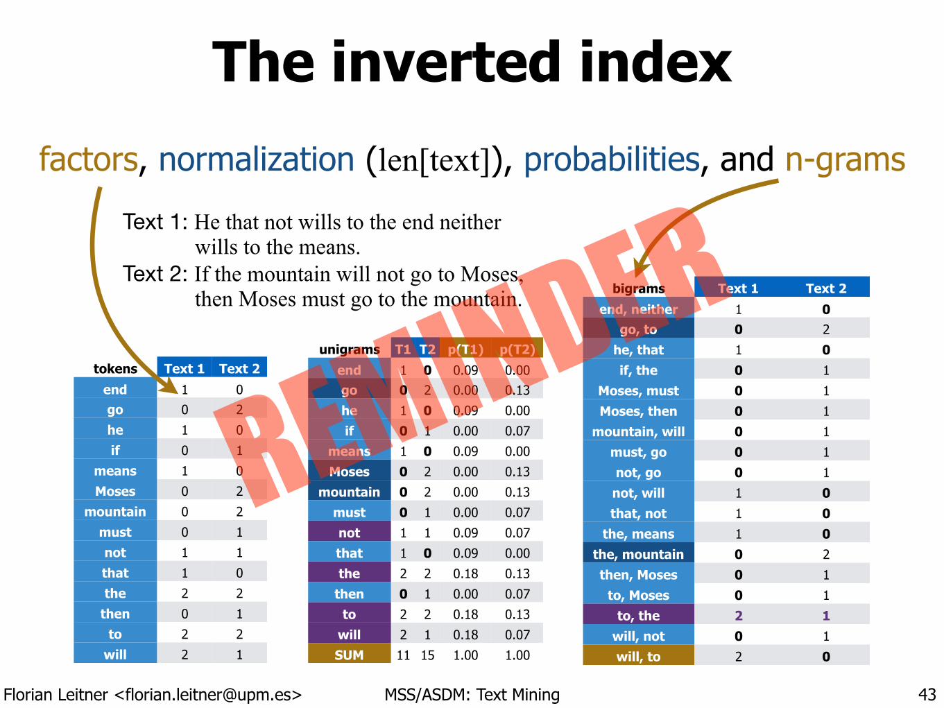
The inverted index
43
Text 1: He that not wills to the end neither wills to the means. Text 2: If the mountain will not go to Moses, then Moses must go to the mountain.
tokens Text 1 Text 2
end 1 0go 0 2
he 1 0
if 0 1
means 1 0
Moses 0 2
mountain 0 2
must 0 1
not 1 1
that 1 0
the 2 2
then 0 1
to 2 2
will 2 1
unigrams T11
T2 p(T1) p(T2)
end 1 0 0.09 0.00go 0 2 0.00 0.13
he 1 0 0.09 0.00
if 0 1 0.00 0.07
means 1 0 0.09 0.00
Moses 0 2 0.00 0.13
mountain 0 2 0.00 0.13
must 0 1 0.00 0.07
not 1 1 0.09 0.07
that 1 0 0.09 0.00
the 2 2 0.18 0.13
then 0 1 0.00 0.07
to 2 2 0.18 0.13
will 2 1 0.18 0.07
SUM 11 15 1.00 1.00
bigrams Text 1 Text 2
end, neither 1 0go, to 0 2
he, that 1 0if, the 0 1
Moses, must 0 1
Moses, then 0 1
mountain, will 0 1
must, go 0 1
not, go 0 1
not, will 1 0that, not 1 0
the, means 1 0the, mountain 0 2
then, Moses 0 1
to, Moses 0 1
to, the 2 1will, not 0 1
will, to 2 0
factors, normalization (len[text]), probabilities, and n-grams
REMINDER
Florian Leitner <[email protected]> MSS/ASDM: Text Mining
Unseen n-grams and the zero probability issue
• Even for unigrams, unseen words will occur sooner or later
• The longer the n-grams, the sooner unseen cases will occur
• “Colorless green ideas sleep furiously.” (Chomsky, 1955)
• As unseen tokens have zero probability, the probability of the whole sentence P(W) = 0 would become zero, too
!
‣ Intuition/idea: Divert a bit of the overall probability mass of each [seen] token to all possible unseen tokens
• Terminology: model smoothing (Chen & Goodman, 1998)
44
Florian Leitner <[email protected]> MSS/ASDM: Text Mining
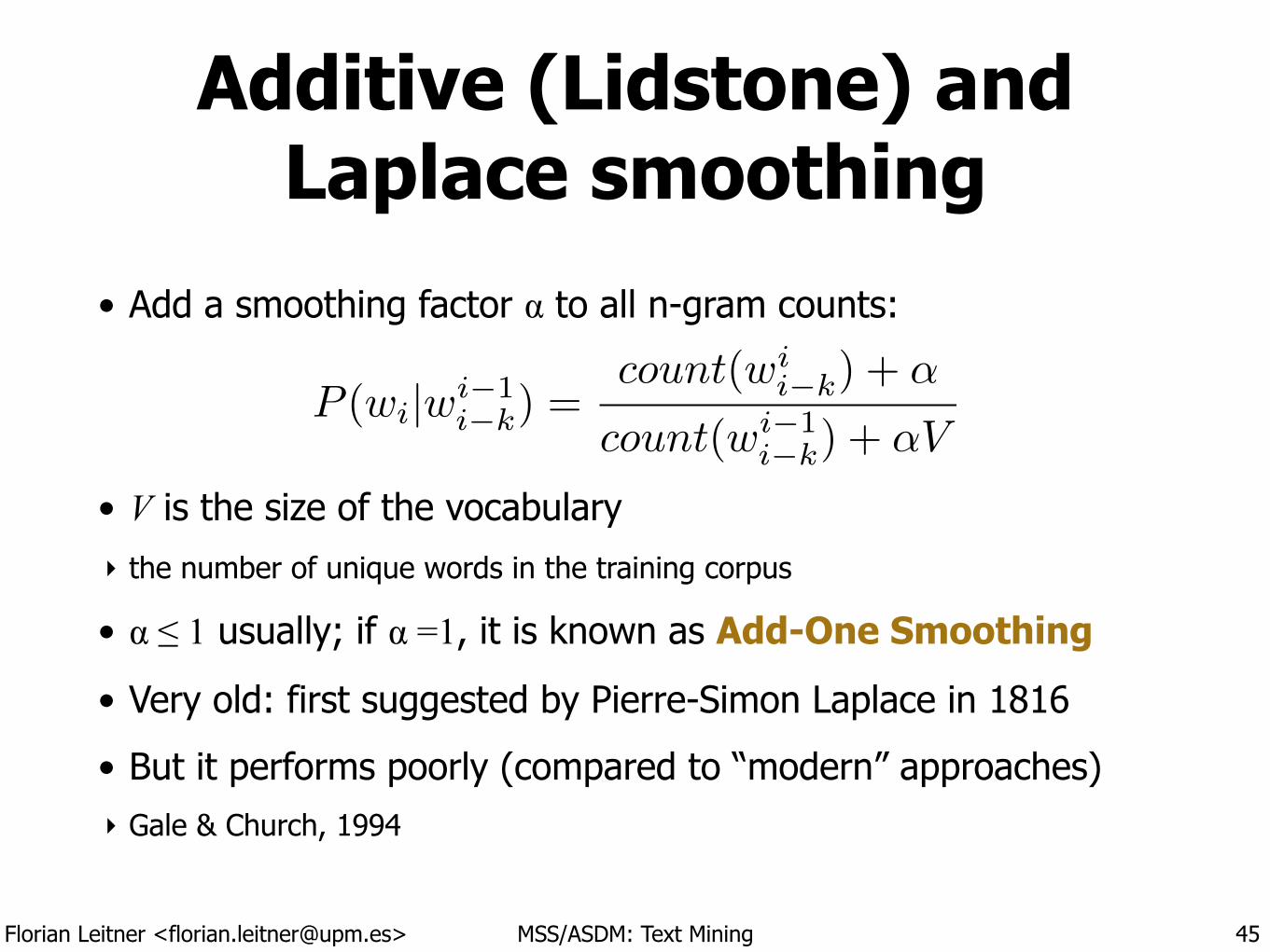
Additive (Lidstone) and Laplace smoothing
• Add a smoothing factor α to all n-gram counts:
!
!
• V is the size of the vocabulary ‣ the number of unique words in the training corpus
• α ≤ 1 usually; if α =1, it is known as Add-One Smoothing
• Very old: first suggested by Pierre-Simon Laplace in 1816
• But it performs poorly (compared to “modern” approaches) ‣ Gale & Church, 1994
45
P (wi|wi�1i�k) =
count(wii�k) + ↵
count(wi�1i�k) + ↵V
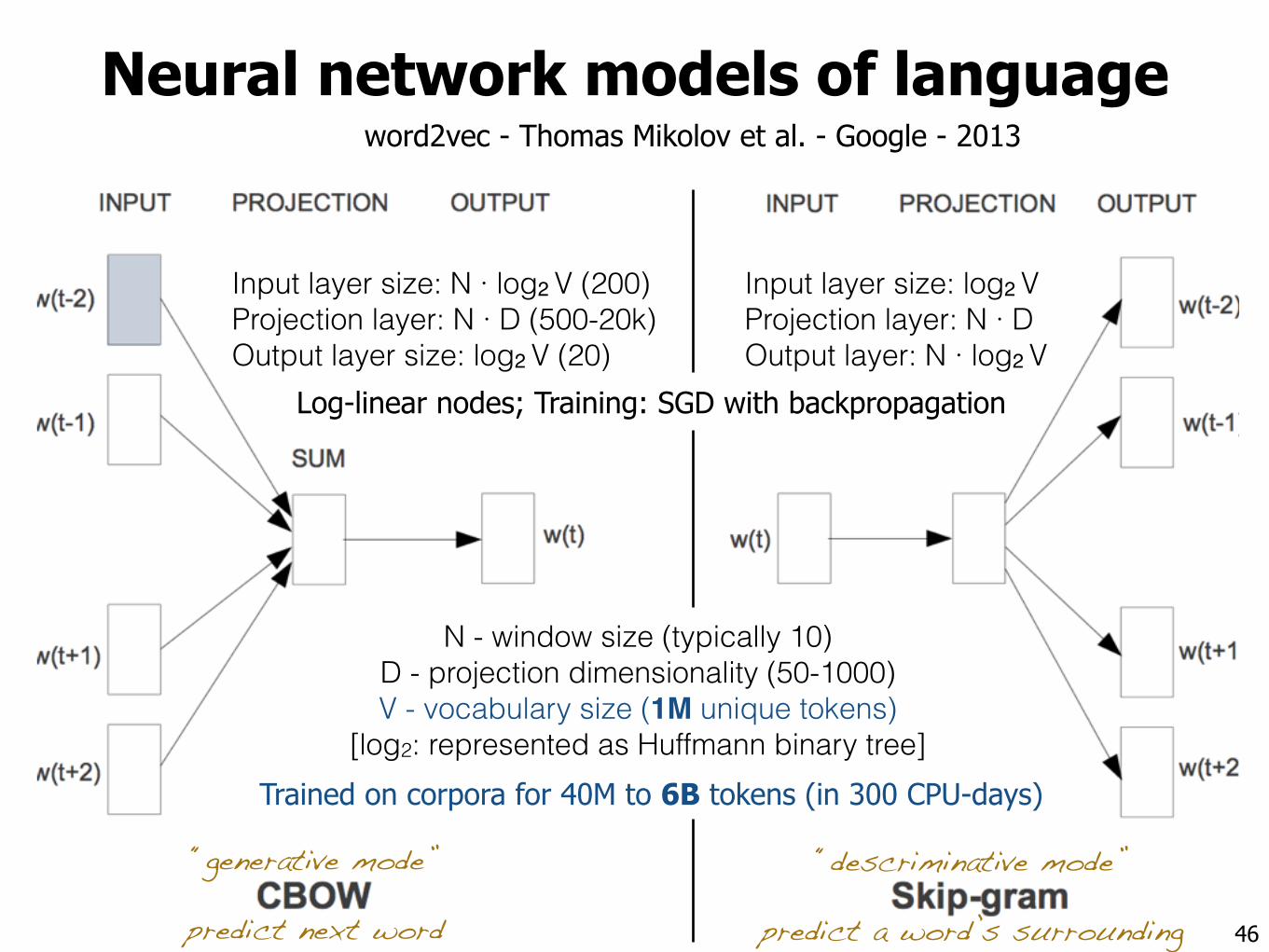
Neural network models of language
46
Log-linear nodes; Training: SGD with backpropagation
Input layer size: log2 V Projection layer: N ∙ D Output layer: N ∙ log2 V
Input layer size: N ∙ log2 V (200) Projection layer: N ∙ D (500-20k) Output layer size: log2 V (20)
N - window size (typically 10) D - projection dimensionality (50-1000) V - vocabulary size (1M unique tokens)
[log2: represented as Huffmann binary tree]
“generative mode” !
predict next word
“descriminative mode”
predict a word’s surrounding
Trained on corpora for 40M to 6B tokens (in 300 CPU-days)
word2vec - Thomas Mikolov et al. - Google - 2013
Florian Leitner <[email protected]> MSS/ASDM: Text Mining
Statistical models of language and polysemy
• Polysemous words have multiple meanings (e.g., “bank”). ‣ This is a real problem in scientific texts because polysemy is frequent.
• One idea: Create context vectors for each sense of a word (vector).
‣ MSSG - Neelakantan et al. - 2015
• Caveat: Performance isn’t much better than for the skip-gram model by Mikolov et al., while training is ~5x slower.
47
Florian Leitner <[email protected]> MSS/ASDM: Text Mining
Neural embeddings: Applications in TM & NLP
• Opinion mining (Maas et al., 2011)
• Paraphrase detection (Socher et al., 2011)
• Chunking (Turian et al., 2010; Dhillon and Ungar, 2011)
• Named entity recognition (Neelakantan and Collins, 2014; Passos et al., 2014; Turian et al., 2010)
• Dependency parsing (Bansal et al., 2014)
48
Florian Leitner <[email protected]> MSS/ASDM: Text Mining
Language model evaluation
• How good is the model you just trained?
• Did your update to the model do any good…?
• Is your model better than someone else’s? ‣ NB: You should compare on the same test set!
49
Florian Leitner <[email protected]> MSS/ASDM: Text Mining
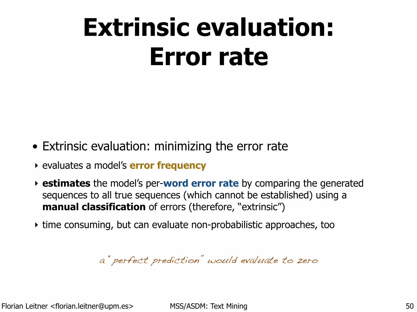
Extrinsic evaluation: Error rate
• Extrinsic evaluation: minimizing the error rate ‣ evaluates a model’s error frequency
‣ estimates the model’s per-word error rate by comparing the generated sequences to all true sequences (which cannot be established) using a manual classification of errors (therefore, “extrinsic”)
‣ time consuming, but can evaluate non-probabilistic approaches, too
50
a “perfect prediction” would evaluate to zero
Florian Leitner <[email protected]> MSS/ASDM: Text Mining
Intrinsic evaluation: Cross-entropy
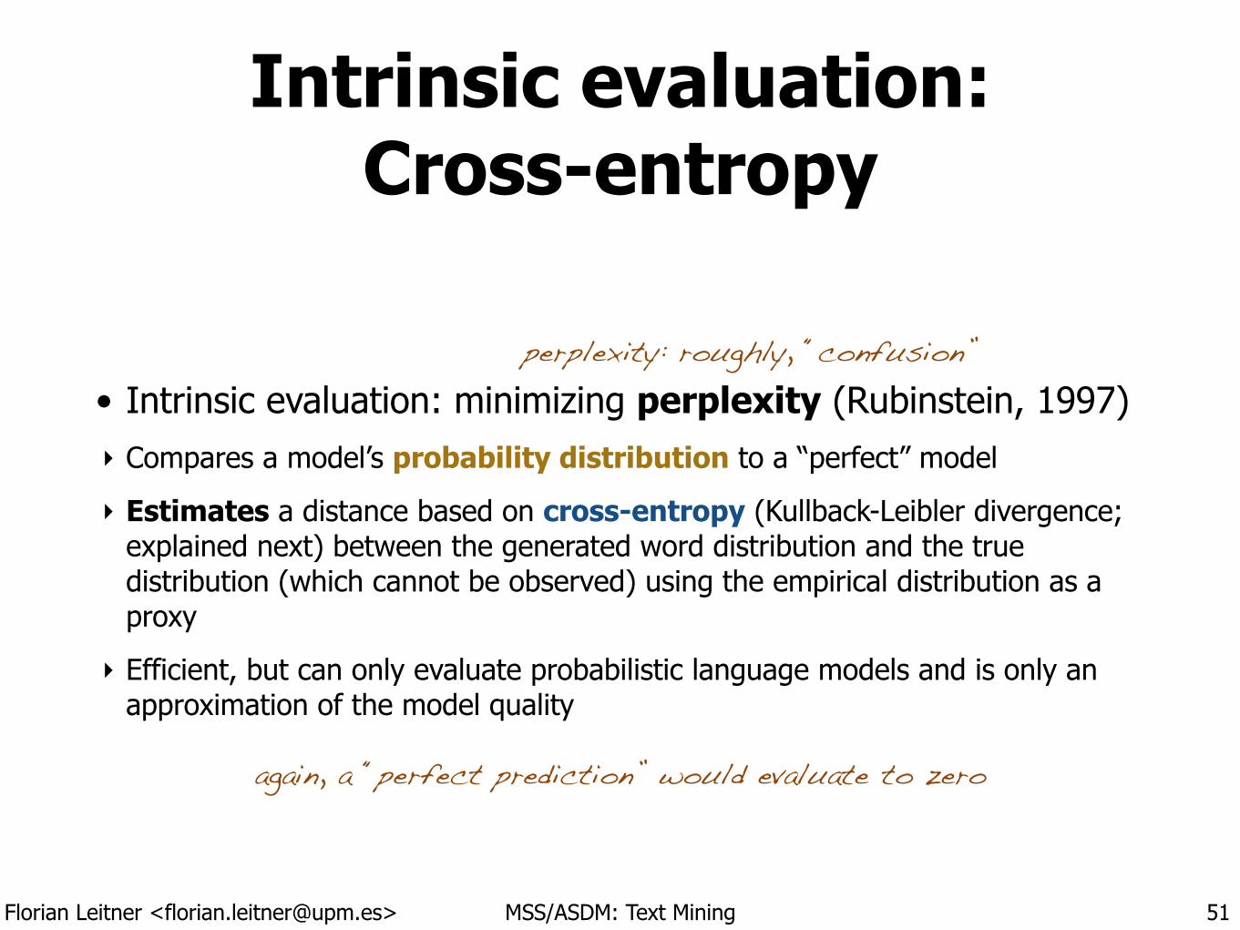
• Intrinsic evaluation: minimizing perplexity (Rubinstein, 1997) ‣ Compares a model’s probability distribution to a “perfect” model
‣ Estimates a distance based on cross-entropy (Kullback-Leibler divergence; explained next) between the generated word distribution and the true distribution (which cannot be observed) using the empirical distribution as a proxy
‣ Efficient, but can only evaluate probabilistic language models and is only an approximation of the model quality
51
again, a “perfect prediction” would evaluate to zero
perplexity: roughly, “confusion”
Florian Leitner <[email protected]> MSS/ASDM: Text Mining
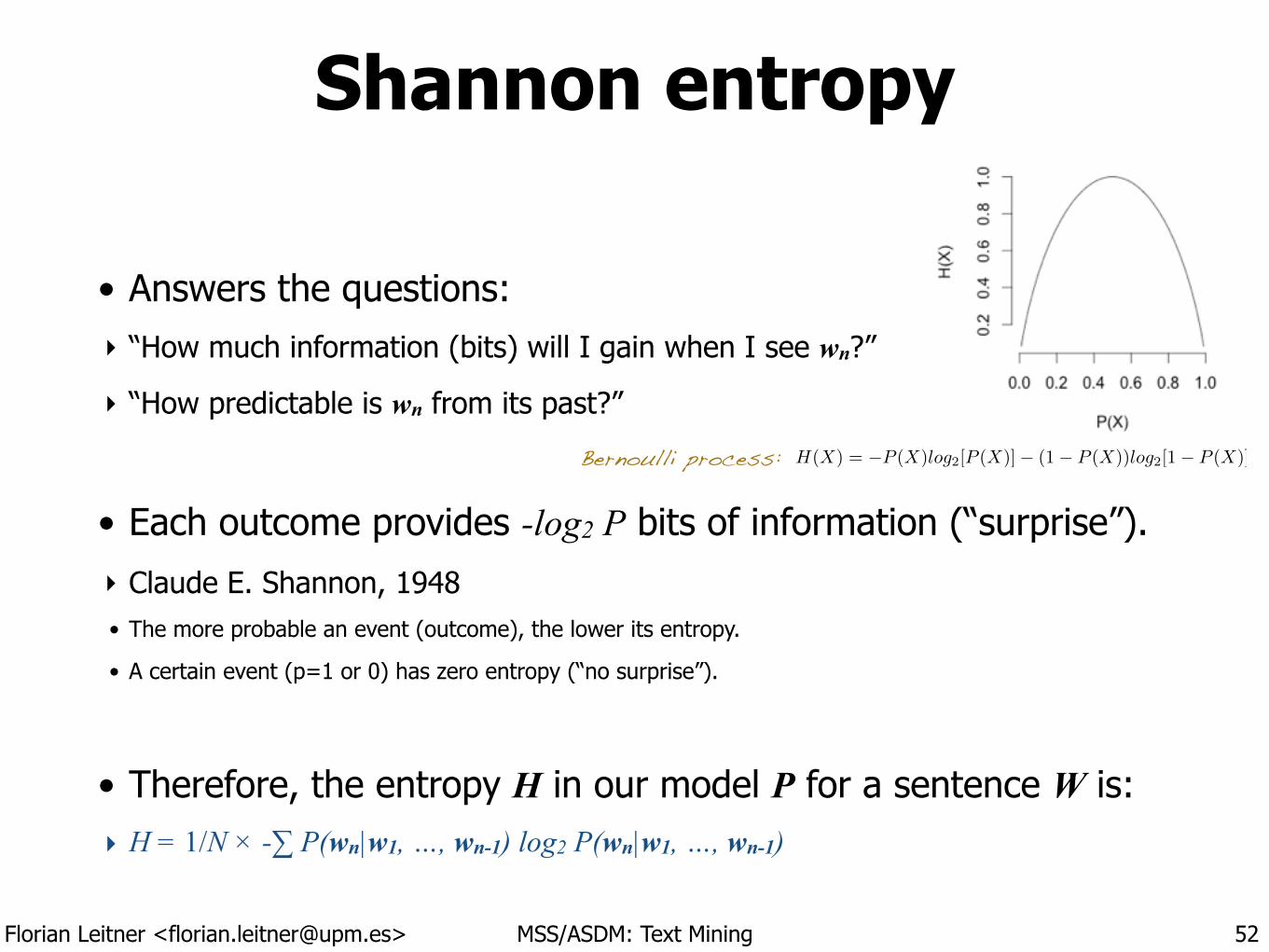
• Answers the questions: ‣ “How much information (bits) will I gain when I see wn?”
‣ “How predictable is wn from its past?”
!
• Each outcome provides -log2 P bits of information (“surprise”). ‣ Claude E. Shannon, 1948 • The more probable an event (outcome), the lower its entropy.
• A certain event (p=1 or 0) has zero entropy (“no surprise”).
!
• Therefore, the entropy H in our model P for a sentence W is: ‣ H = 1/N × -∑ P(wn|w1, …, wn-1) log2 P(wn|w1, …, wn-1)
Shannon entropy
52
H(X) = �P (X)log2[P (X)]� (1� P (X))log2[1� P (X)]Bernoulli process:
Florian Leitner <[email protected]> MSS/ASDM: Text Mining
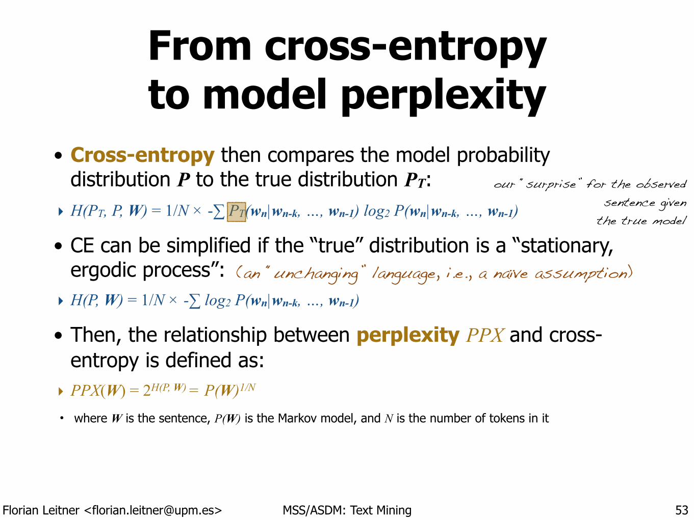
From cross-entropy to model perplexity
• Cross-entropy then compares the model probability distribution P to the true distribution PT:
‣ H(PT, P, W) = 1/N × -∑ PT(wn|wn-k, …, wn-1) log2 P(wn|wn-k, …, wn-1)
• CE can be simplified if the “true” distribution is a “stationary, ergodic process”:
‣ H(P, W) = 1/N × -∑ log2 P(wn|wn-k, …, wn-1)
• Then, the relationship between perplexity PPX and cross-entropy is defined as:
‣ PPX(W) = 2H(P, W) = P(W)1/N
• where W is the sentence, P(W) is the Markov model, and N is the number of tokens in it
53
(an “unchanging” language, i.e., a naïve assumption)
our “surprise” for the observed sentence given
the true model
Florian Leitner <[email protected]> MSS/ASDM: Text Mining
Interpreting perplexity
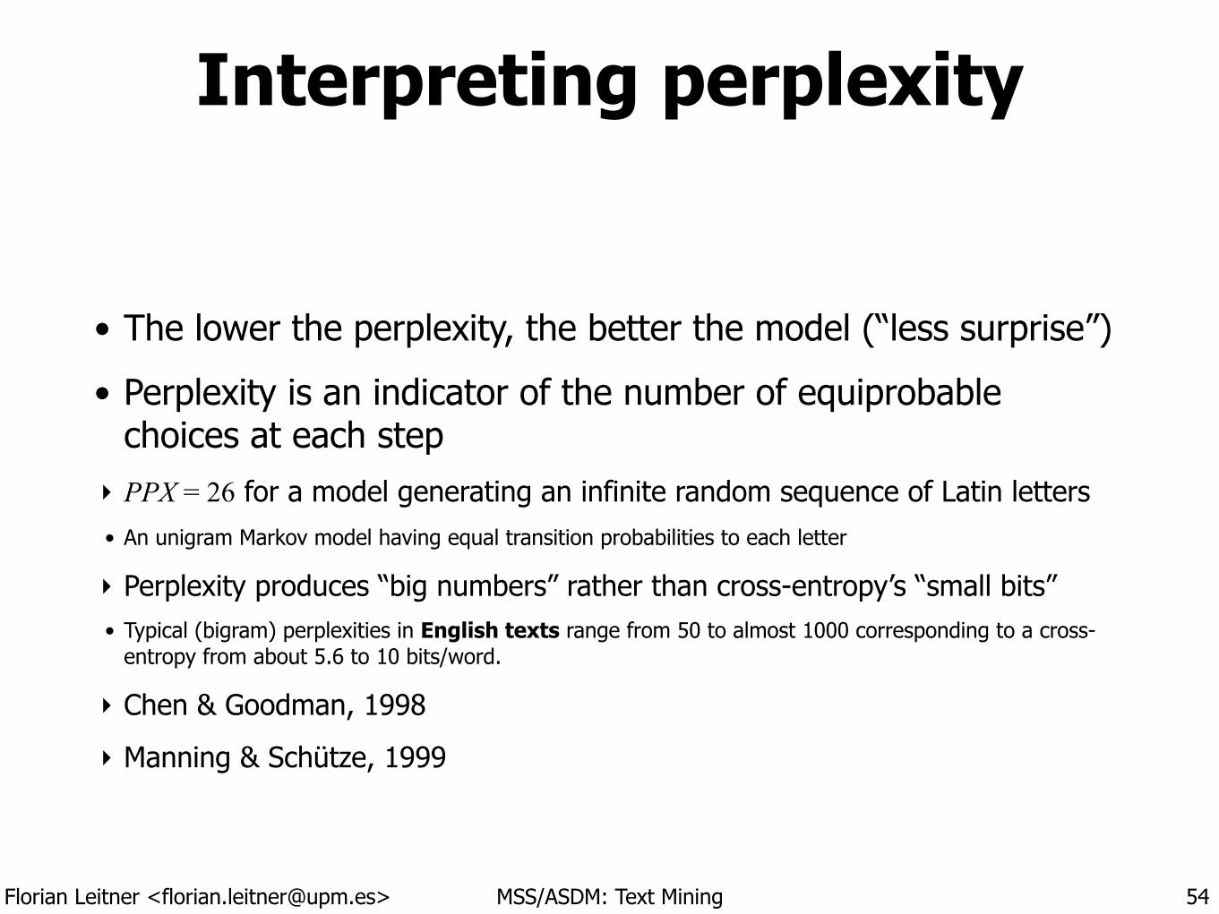
• The lower the perplexity, the better the model (“less surprise”)
• Perplexity is an indicator of the number of equiprobable choices at each step
‣ PPX = 26 for a model generating an infinite random sequence of Latin letters • An unigram Markov model having equal transition probabilities to each letter
‣ Perplexity produces “big numbers” rather than cross-entropy’s “small bits” • Typical (bigram) perplexities in English texts range from 50 to almost 1000 corresponding to a cross-
entropy from about 5.6 to 10 bits/word.
‣ Chen & Goodman, 1998
‣ Manning & Schütze, 1999
54
Text Mining 3 Text Similarity
!Madrid Summer School on
Advanced Statistics and Data Mining !
Florian Leitner [email protected]
License:
Florian Leitner <[email protected]> MSS/ASDM: Text Mining
Incentive and applications
• Goals of string similarity matching: ‣ Detecting syntactically or semantically similar words
!
• Grouping/clustering similar items ‣ Content-based recommender systems; plagiarism detection
• Information retrieval ‣ Ranking/searching for [query-specific] documents
• Entity grounding ‣ Recognizing entities from a collection of strings (a “gazetteer” or dictionary)
56
Florian Leitner <[email protected]> MSS/ASDM: Text Mining
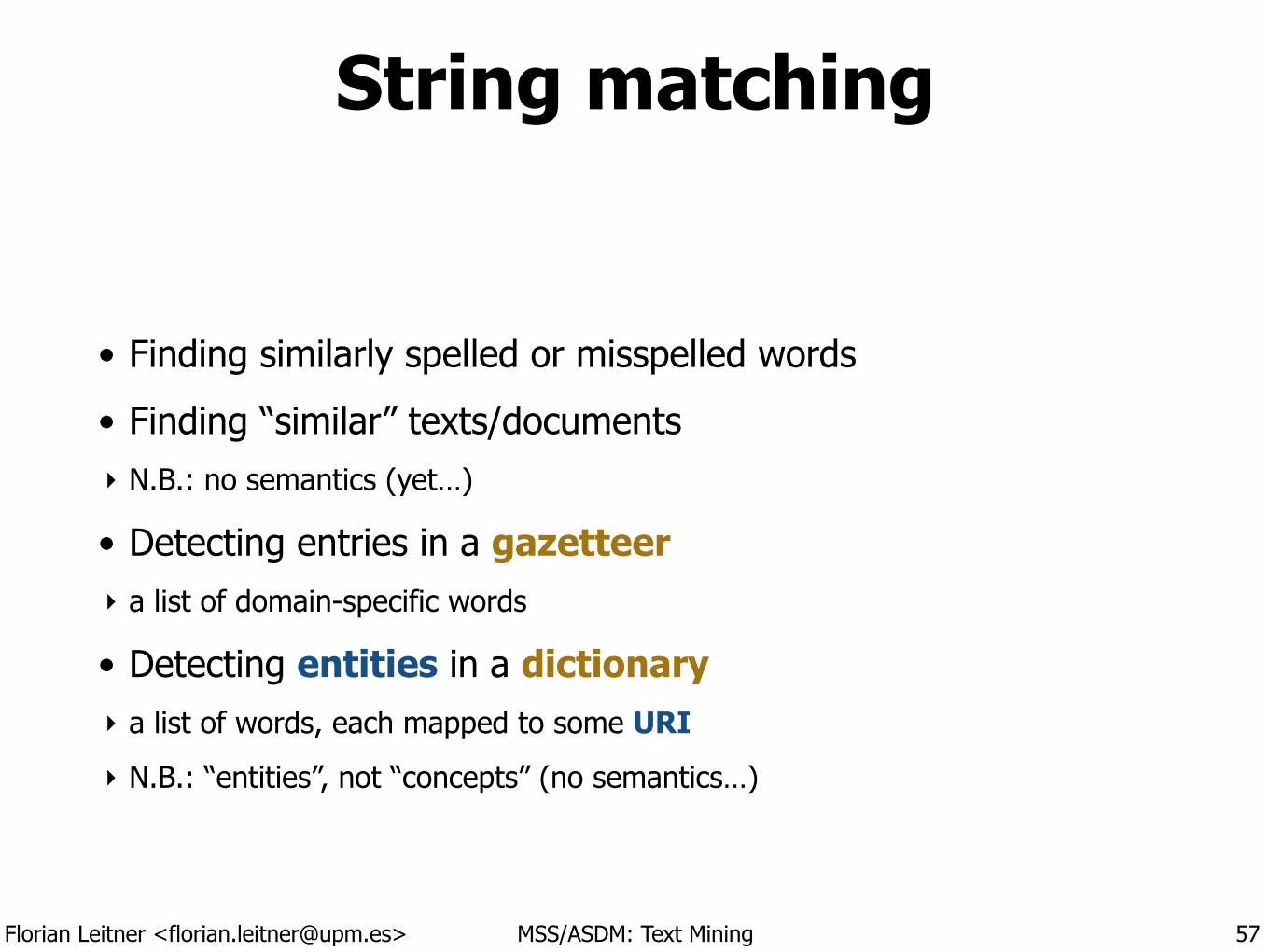
• Finding similarly spelled or misspelled words
• Finding “similar” texts/documents ‣ N.B.: no semantics (yet…)
• Detecting entries in a gazetteer ‣ a list of domain-specific words
• Detecting entities in a dictionary ‣ a list of words, each mapped to some URI
‣ N.B.: “entities”, not “concepts” (no semantics…)
String matching
57
Florian Leitner <[email protected]> MSS/ASDM: Text Mining
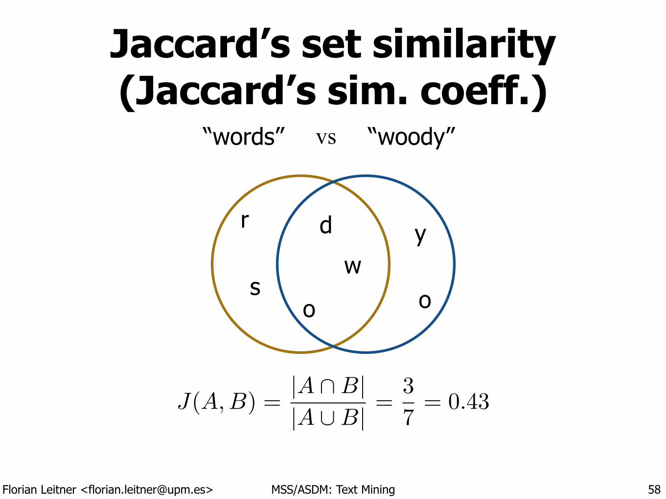
Jaccard’s set similarity(Jaccard’s sim. coeff.)
58
“words” “woody”
w
o
r
s
d y
J(A,B) =|A \B||A [B| =
3
7= 0.43
vs
o
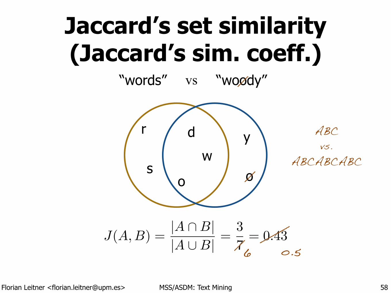
Florian Leitner <[email protected]> MSS/ASDM: Text Mining
Jaccard’s set similarity(Jaccard’s sim. coeff.)
58
“words” “woody”
w
o
r
s
d y
J(A,B) =|A \B||A [B| =
3
7= 0.43
vs
o
6 o.5
ABC vs.
ABCABCABC
Florian Leitner <[email protected]> MSS/ASDM: Text Mining
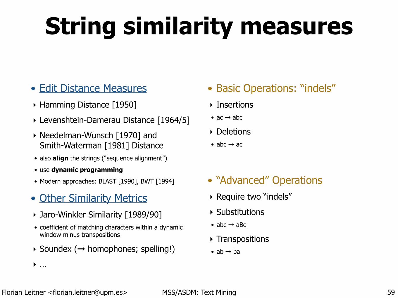
String similarity measures
• Edit Distance Measures ‣ Hamming Distance [1950]
‣ Levenshtein-Damerau Distance [1964/5]
‣ Needelman-Wunsch [1970] and Smith-Waterman [1981] Distance
• also align the strings (“sequence alignment”)
• use dynamic programming
• Modern approaches: BLAST [1990], BWT [1994]
• Other Similarity Metrics ‣ Jaro-Winkler Similarity [1989/90] • coefficient of matching characters within a dynamic
window minus transpositions
‣ Soundex (➞ homophones; spelling!)
‣ …
• Basic Operations: “indels” ‣ Insertions • ac ➞ abc
‣ Deletions • abc ➞ ac
!
• “Advanced” Operations ‣ Require two “indels”
‣ Substitutions • abc ➞ aBc
‣ Transpositions • ab ➞ ba
59
Florian Leitner <[email protected]> MSS/ASDM: Text Mining
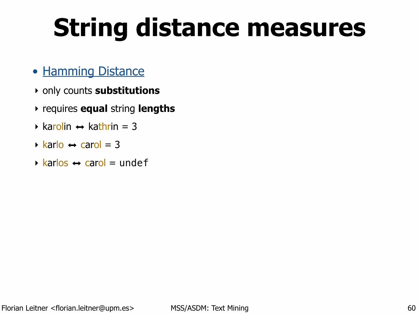
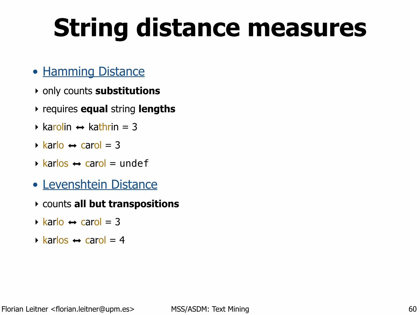
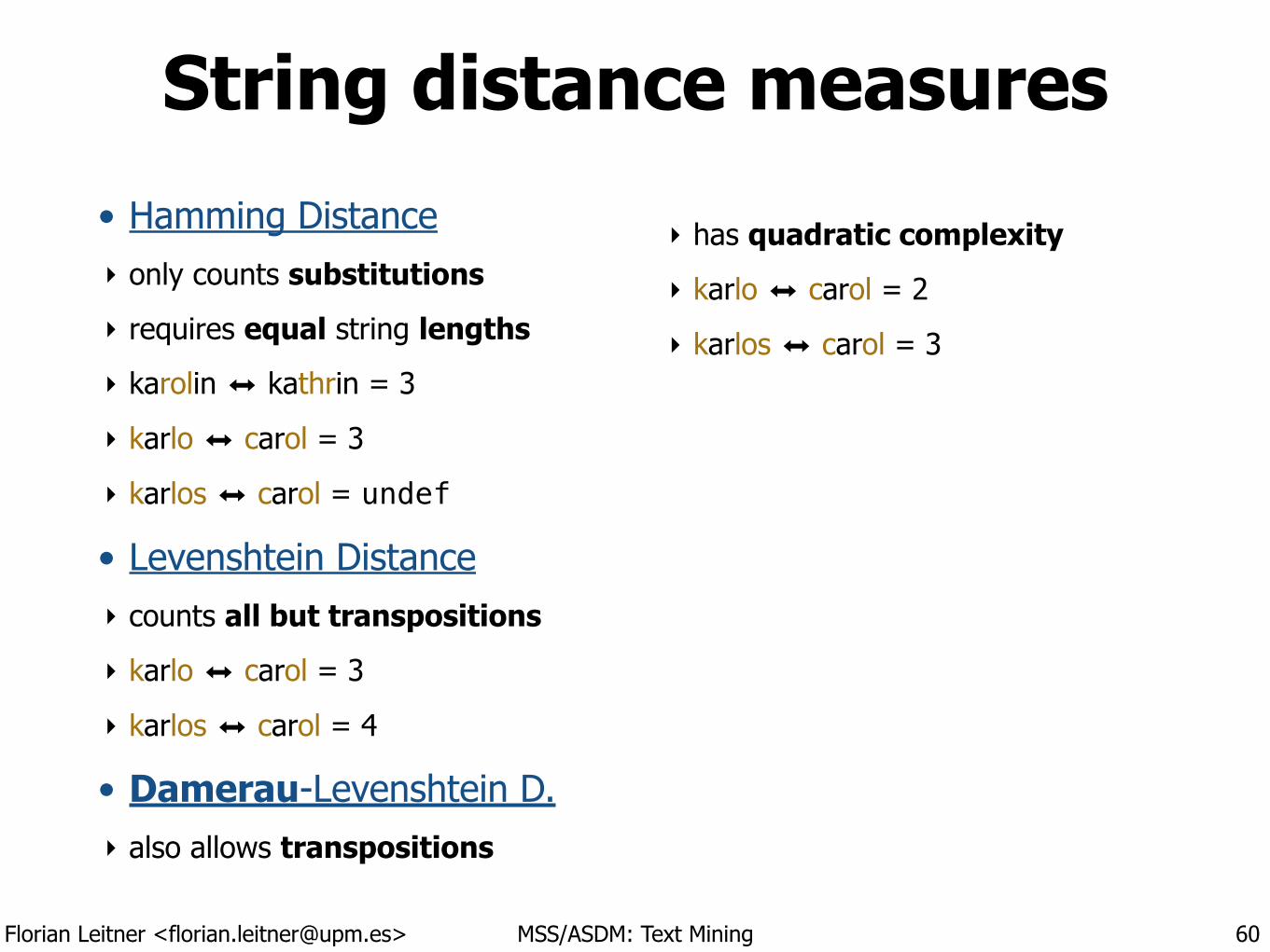
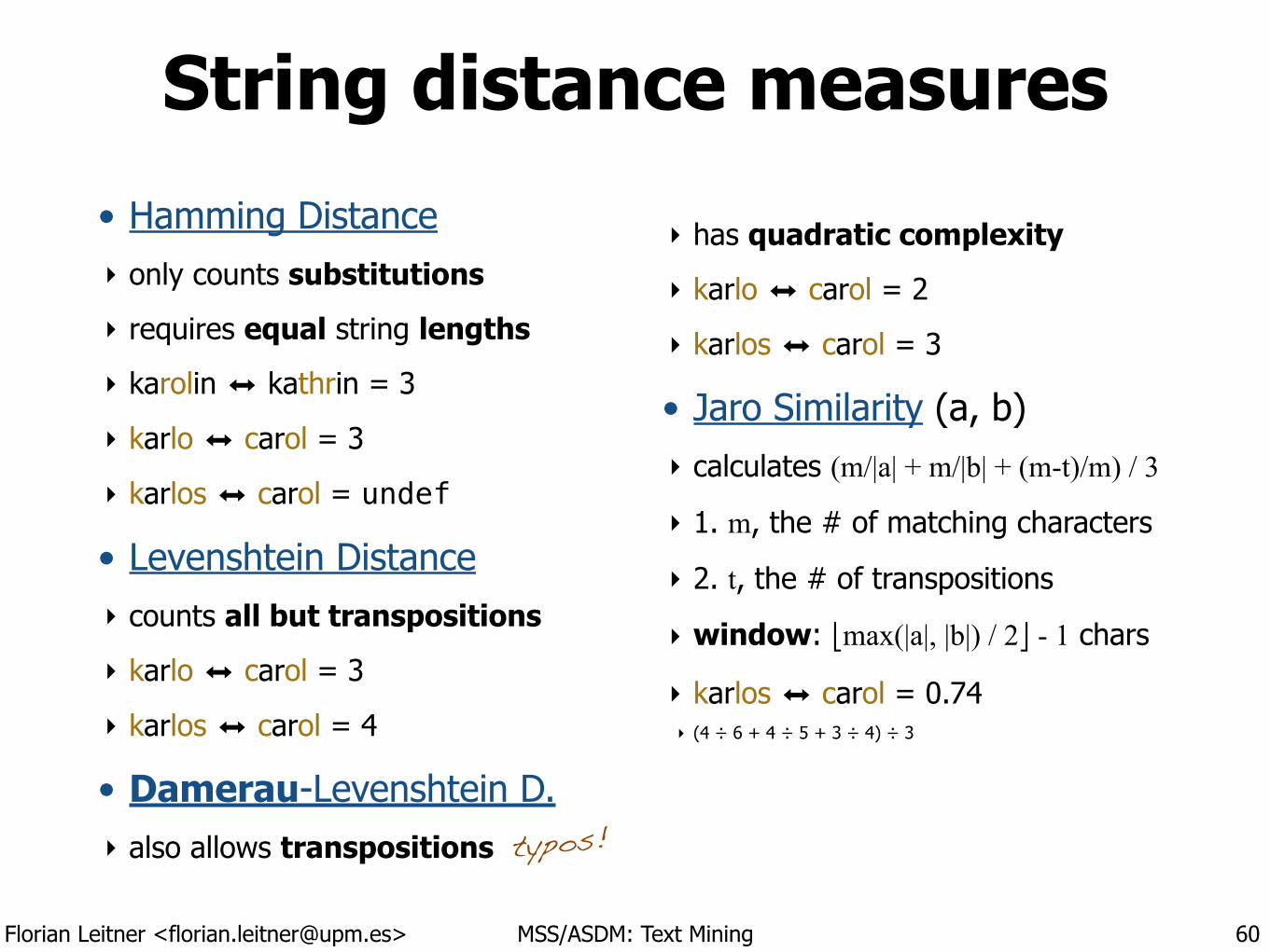
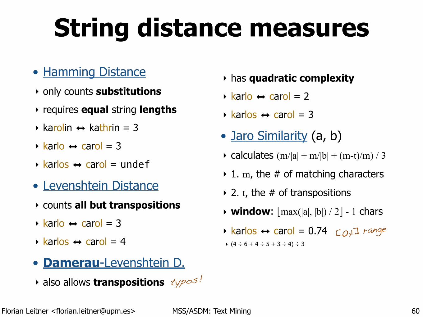
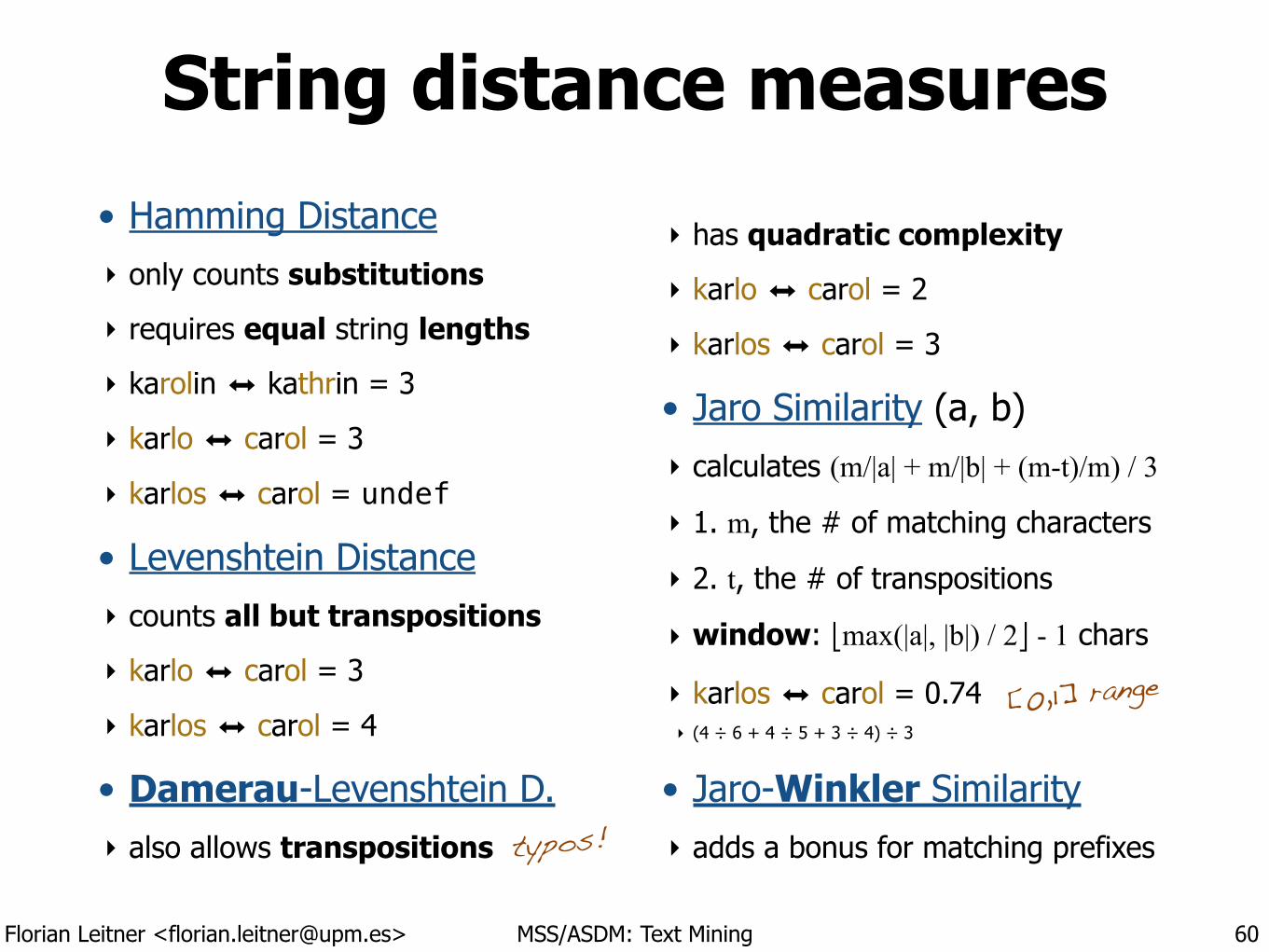
String distance measures• Hamming Distance ‣ only counts substitutions
‣ requires equal string lengths
‣ karolin ⬌ kathrin = 3
‣ karlo ⬌ carol = 3
‣ karlos ⬌ carol = undef
60
Florian Leitner <[email protected]> MSS/ASDM: Text Mining
String distance measures• Hamming Distance ‣ only counts substitutions
‣ requires equal string lengths
‣ karolin ⬌ kathrin = 3
‣ karlo ⬌ carol = 3
‣ karlos ⬌ carol = undef
• Levenshtein Distance ‣ counts all but transpositions
‣ karlo ⬌ carol = 3
‣ karlos ⬌ carol = 4
• Damerau-Levenshtein D. ‣ also allows transpositions
‣ has quadratic complexity
‣ karlo ⬌ carol = 2
‣ karlos ⬌ carol = 3
60
typos!
Florian Leitner <[email protected]> MSS/ASDM: Text Mining
String distance measures• Hamming Distance ‣ only counts substitutions
‣ requires equal string lengths
‣ karolin ⬌ kathrin = 3
‣ karlo ⬌ carol = 3
‣ karlos ⬌ carol = undef
• Levenshtein Distance ‣ counts all but transpositions
‣ karlo ⬌ carol = 3
‣ karlos ⬌ carol = 4
• Damerau-Levenshtein D. ‣ also allows transpositions
‣ has quadratic complexity
‣ karlo ⬌ carol = 2
‣ karlos ⬌ carol = 3
• Jaro Similarity (a, b) ‣ calculates (m/|a| + m/|b| + (m-t)/m) / 3
‣ 1. m, the # of matching characters
‣ 2. t, the # of transpositions
‣ window: !max(|a|, |b|) / 2" - 1 chars
‣ karlos ⬌ carol = 0.74 ‣ (4 ÷ 6 + 4 ÷ 5 + 3 ÷ 4) ÷ 3
60
[0,1] range
typos!
Florian Leitner <[email protected]> MSS/ASDM: Text Mining
String distance measures• Hamming Distance ‣ only counts substitutions
‣ requires equal string lengths
‣ karolin ⬌ kathrin = 3
‣ karlo ⬌ carol = 3
‣ karlos ⬌ carol = undef
• Levenshtein Distance ‣ counts all but transpositions
‣ karlo ⬌ carol = 3
‣ karlos ⬌ carol = 4
• Damerau-Levenshtein D. ‣ also allows transpositions
‣ has quadratic complexity
‣ karlo ⬌ carol = 2
‣ karlos ⬌ carol = 3
• Jaro Similarity (a, b) ‣ calculates (m/|a| + m/|b| + (m-t)/m) / 3
‣ 1. m, the # of matching characters
‣ 2. t, the # of transpositions
‣ window: !max(|a|, |b|) / 2" - 1 chars
‣ karlos ⬌ carol = 0.74 ‣ (4 ÷ 6 + 4 ÷ 5 + 3 ÷ 4) ÷ 3
• Jaro-Winkler Similarity ‣ adds a bonus for matching prefixes
60
[0,1] range
typos!
Florian Leitner <[email protected]> MSS/ASDM: Text Mining
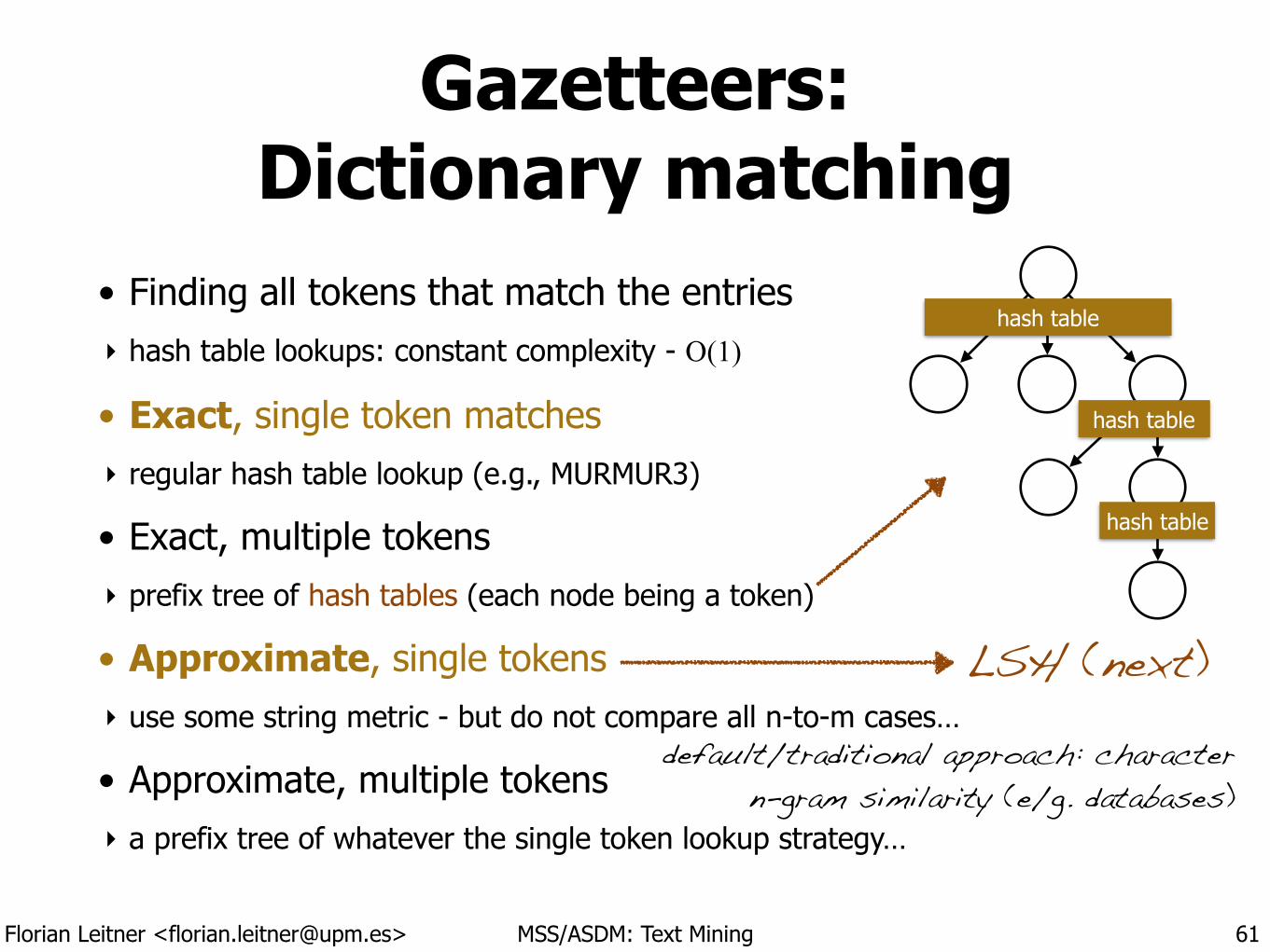
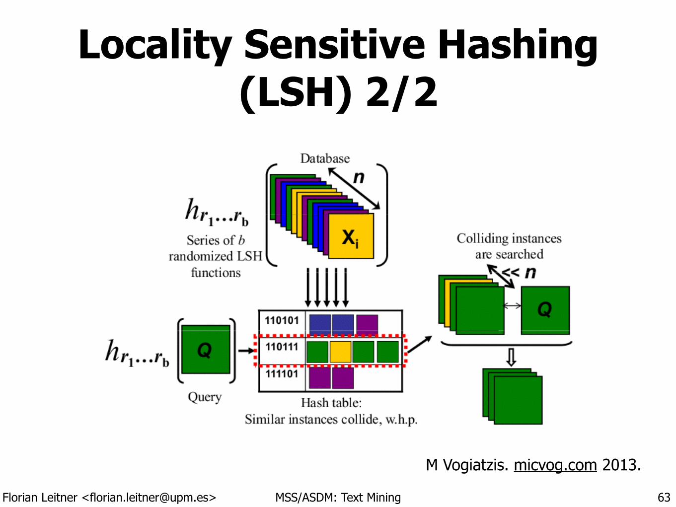
Gazetteers: Dictionary matching
• Finding all tokens that match the entries ‣ hash table lookups: constant complexity - O(1)
• Exact, single token matches ‣ regular hash table lookup (e.g., MURMUR3)
• Exact, multiple tokens ‣ prefix tree of hash tables (each node being a token)
• Approximate, single tokens ‣ use some string metric - but do not compare all n-to-m cases…
• Approximate, multiple tokens ‣ a prefix tree of whatever the single token lookup strategy…
61
LSH (next)
hash table
hash table
hash table
default/traditional approach: character n-gram similarity (e/g. databases)
Florian Leitner <[email protected]> MSS/ASDM: Text Mining
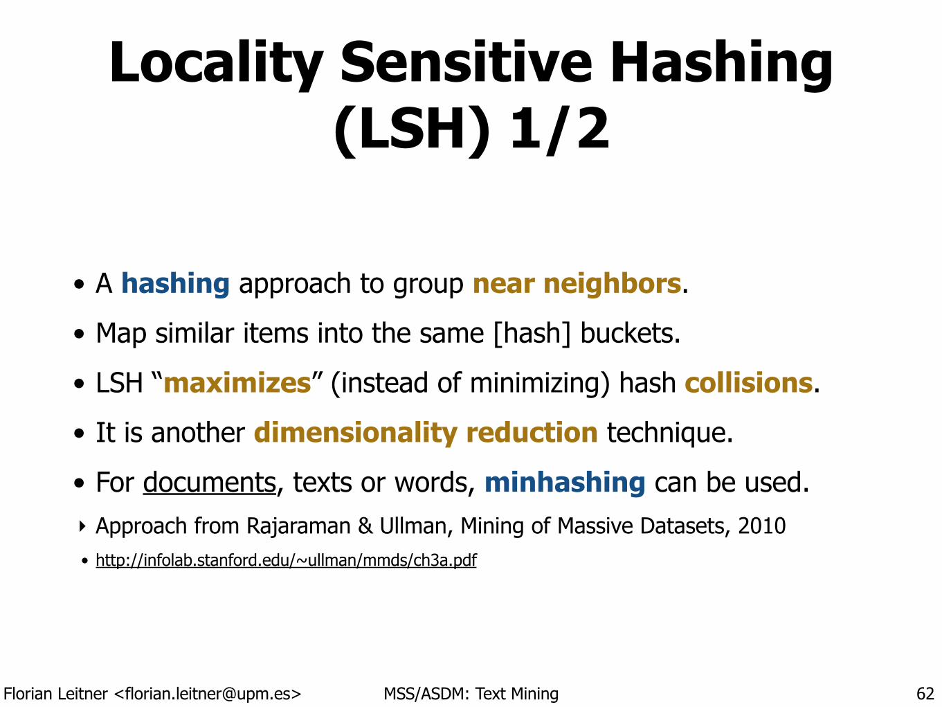
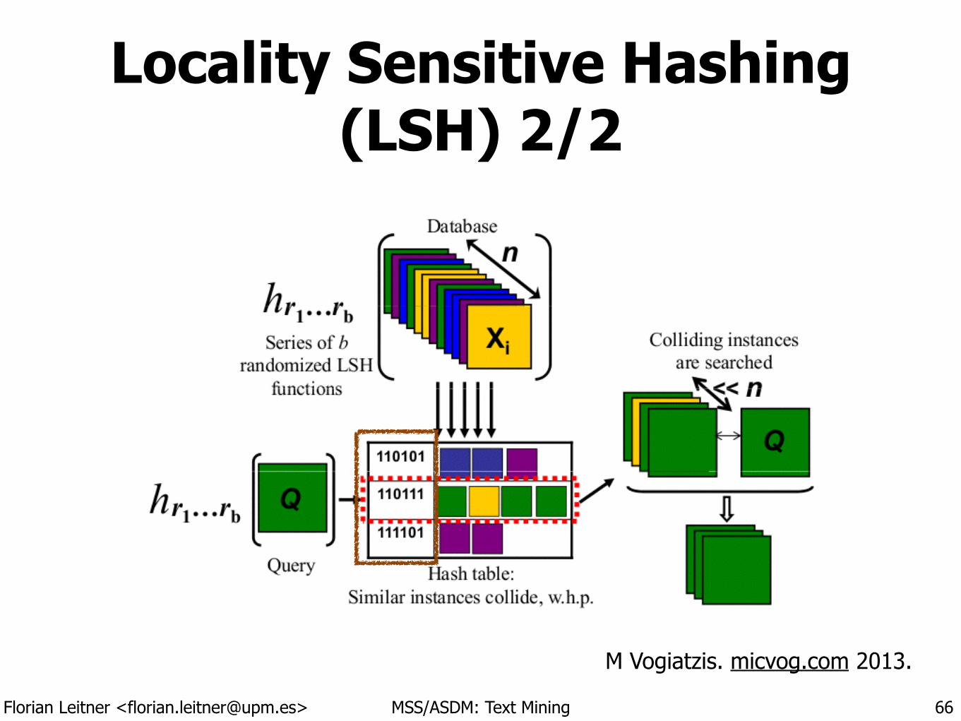
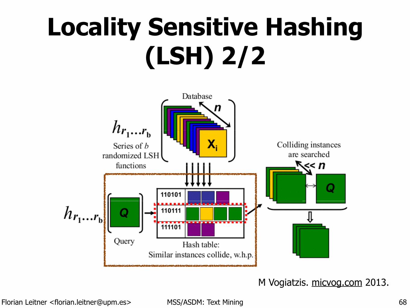
Locality Sensitive Hashing (LSH) 1/2
• A hashing approach to group near neighbors.
• Map similar items into the same [hash] buckets.
• LSH “maximizes” (instead of minimizing) hash collisions.
• It is another dimensionality reduction technique.
• For documents, texts or words, minhashing can be used. ‣ Approach from Rajaraman & Ullman, Mining of Massive Datasets, 2010 • http://infolab.stanford.edu/~ullman/mmds/ch3a.pdf
62
Florian Leitner <[email protected]> MSS/ASDM: Text Mining
Locality Sensitive Hashing (LSH) 2/2
63
M Vogiatzis. micvog.com 2013.
Florian Leitner <[email protected]> MSS/ASDM: Text Mining
Minhash signatures (1/2)
65
shin
gle
or n
-gra
m ID
Create character n-gram × token or word k-shingle × document matrix
(likely very sparse!)
Lemma: Two texts will have the same first “true” shingle/n-gram when looking from top to bottom with a probability equal to their Jaccard (Set) Similarity.
!Idea: Create sufficient permutations of the row (shingle/n-gram) ordering so that the Jaccard Similarity can be approximated by comparing the number of
coinciding vs. differing rows.
01234
TTFFTF
TFFTFF
TFTFTT
TTFTTF
h12340
h14203
a family of hash functions hi
h1(x) = (x+1)%n !
h2(x) = (3x+1)%n !
n=5
T: shingle/n-gram in Ti F: shingle/n-gram not in Ti
“permuted” row IDs
Florian Leitner <[email protected]> MSS/ASDM: Text Mining
Locality Sensitive Hashing (LSH) 2/2
66
M Vogiatzis. micvog.com 2013.
Florian Leitner <[email protected]> MSS/ASDM: Text Mining
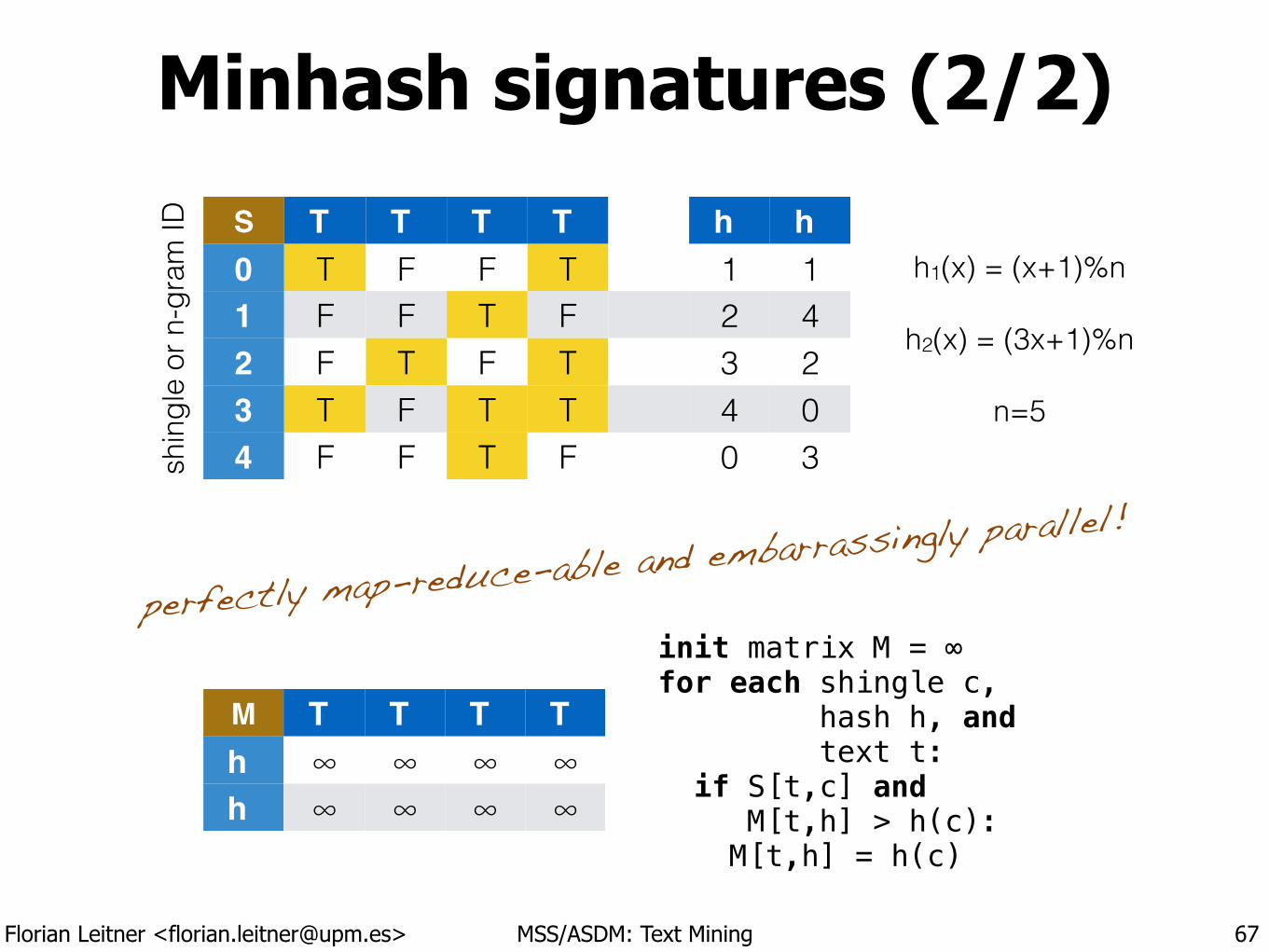
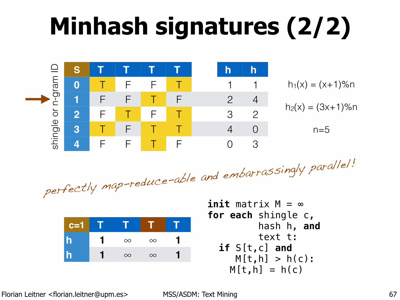
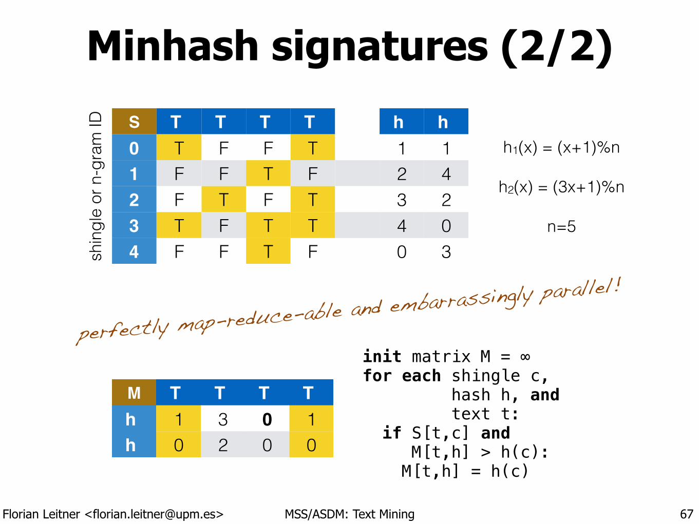
Minhash signatures (2/2)
67
shin
gle
or n
-gra
m ID S T T T T h h
0 T F F T 1 11 F F T F 2 42 F T F T 3 23 T F T T 4 04 F F T F 0 3
h1(x) = (x+1)%n !
h2(x) = (3x+1)%n !
n=5
M T T T Th ∞ ∞ ∞ ∞h ∞ ∞ ∞ ∞
init matrix M = ∞ for each shingle c, hash h, and text t: if S[t,c] and M[t,h] > h(c): M[t,h] = h(c)
perfectly map-reduce-able and embarrassingly parallel!
Florian Leitner <[email protected]> MSS/ASDM: Text Mining
Minhash signatures (2/2)
67
shin
gle
or n
-gra
m ID S T T T T h h
0 T F F T 1 11 F F T F 2 42 F T F T 3 23 T F T T 4 04 F F T F 0 3
h1(x) = (x+1)%n !
h2(x) = (3x+1)%n !
n=5
M T T T Th ∞ ∞ ∞ ∞h ∞ ∞ ∞ ∞
init matrix M = ∞ for each shingle c, hash h, and text t: if S[t,c] and M[t,h] > h(c): M[t,h] = h(c)
perfectly map-reduce-able and embarrassingly parallel!
c=0 T T T Th ∞ ∞ ∞ ∞h ∞ ∞ ∞ ∞
c=1 T T T Th 1 ∞ ∞ 1h 1 ∞ ∞ 1
c=2 T T T Th 1 ∞ 2 1h 1 ∞ 4 1
c=3 T T T Th 1 3 2 1h 1 2 4 1
c=4 T T T Th 1 3 2 1h 0 2 0 0
M T T T Th 1 3 0 1h 0 2 0 0
Florian Leitner <[email protected]> MSS/ASDM: Text Mining
Locality Sensitive Hashing (LSH) 2/2
68
M Vogiatzis. micvog.com 2013.
Florian Leitner <[email protected]> MSS/ASDM: Text Mining
T T T T T T T T …h 1 0 2 1 7 1 4 5h 1 2 4 1 6 5 5 6h 0 5 6 0 6 4 7 9h 4 0 8 8 7 6 5 7h 7 7 0 8 3 8 7 3h 8 9 0 7 2 4 8 2h 8 5 4 0 9 8 4 7h 9 4 3 9 0 8 3 9h 8 5 8 0 0 6 8 0…
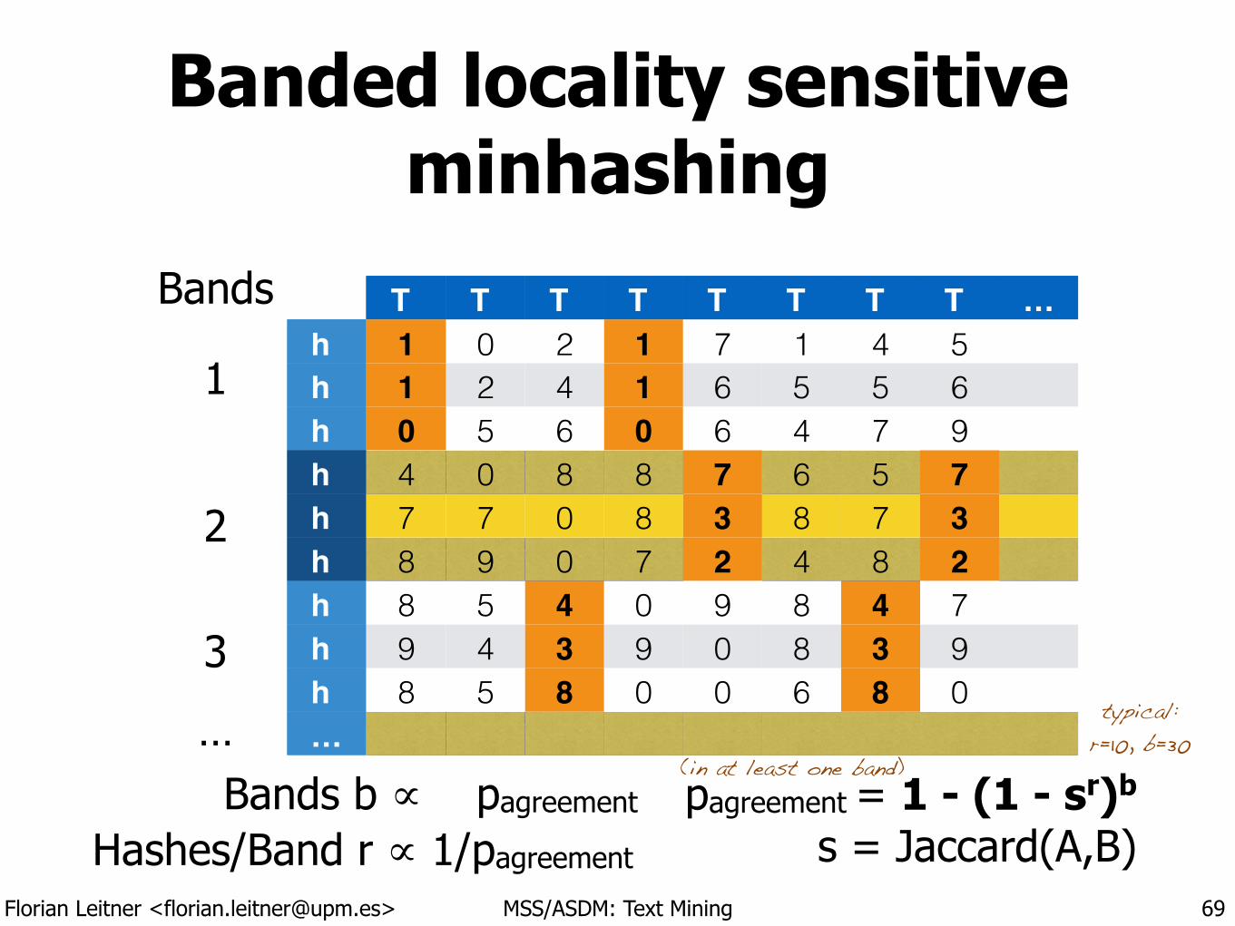
Banded locality sensitive minhashing
69
T T T T T T T T …h 1 0 2 1 7 1 4 5h 1 2 4 1 6 5 5 6h 0 5 6 0 6 4 7 9h 4 0 8 8 7 6 5 7h 7 7 0 8 3 8 7 3h 8 9 0 7 2 4 8 2h 8 5 4 0 9 8 4 7h 9 4 3 9 0 8 3 9h 8 5 8 0 0 6 8 0…
Bands
1
2
3
… Bands b ∝ pagreement Hashes/Band r ∝ 1/pagreement
pagreement = 1 - (1 - sr)b
s = Jaccard(A,B)
(in at least one band)
typical: r=10, b=30
Florian Leitner <[email protected]> MSS/ASDM: Text Mining
Document similarity
• Similarity measures ✓Cosine similarity (of document/text vectors)
‣ Correlation coefficients
• Word vector normalization ‣ TF-IDF
• Dimensionality Reduction/Clustering ✓Locality Sensitivity Hashing
‣ Latent semantic indexing
‣ Latent Dirichlet allocation (tomorrow)
70
Florian Leitner <[email protected]> MSS/ASDM: Text Mining
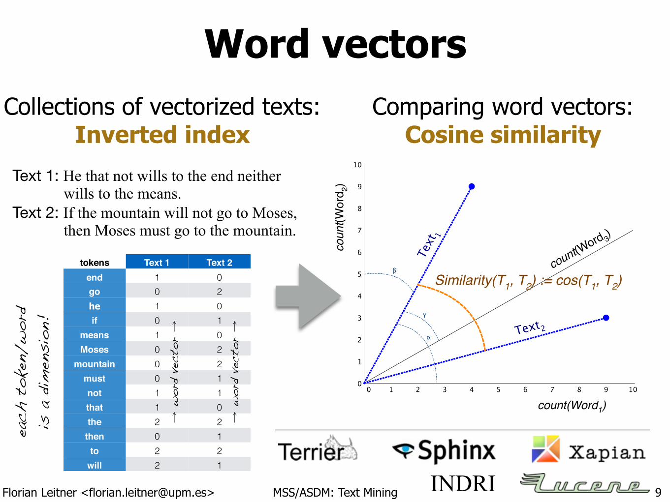
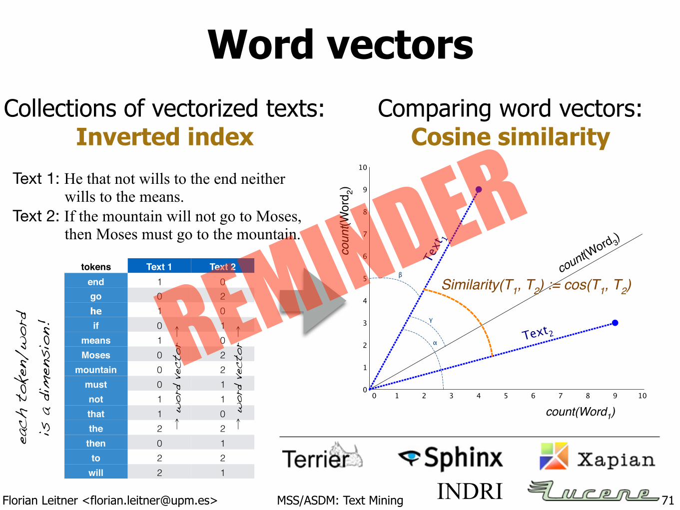
Word vectors
71
0 1 2 3 4 5 6 7 8 9 10
10
0
1
2
3
4
5
6
7
8
9
count(Word1)
coun
t(Word 2)
Text
1
Text2α
γ
βSimilarity(T1, T2) := cos(T1, T2)
count(Word 3
)
Comparing word vectors: Cosine similarity
Collections of vectorized texts: Inverted index
Text 1: He that not wills to the end neither wills to the means. Text 2: If the mountain will not go to Moses, then Moses must go to the mountain.
tokens Text 1 Text 2end 1 0go 0 2he 1 0if 0 1
means 1 0Moses 0 2
mountain 0 2must 0 1not 1 1that 1 0the 2 2
then 0 1to 2 2
will 2 1
INDRI
each
tok
en/w
ord
is a
dimen
sion!
� w
ord
vecto
r �
� w
ord
vecto
r �REMINDER
Florian Leitner <[email protected]> MSS/ASDM: Text Mining
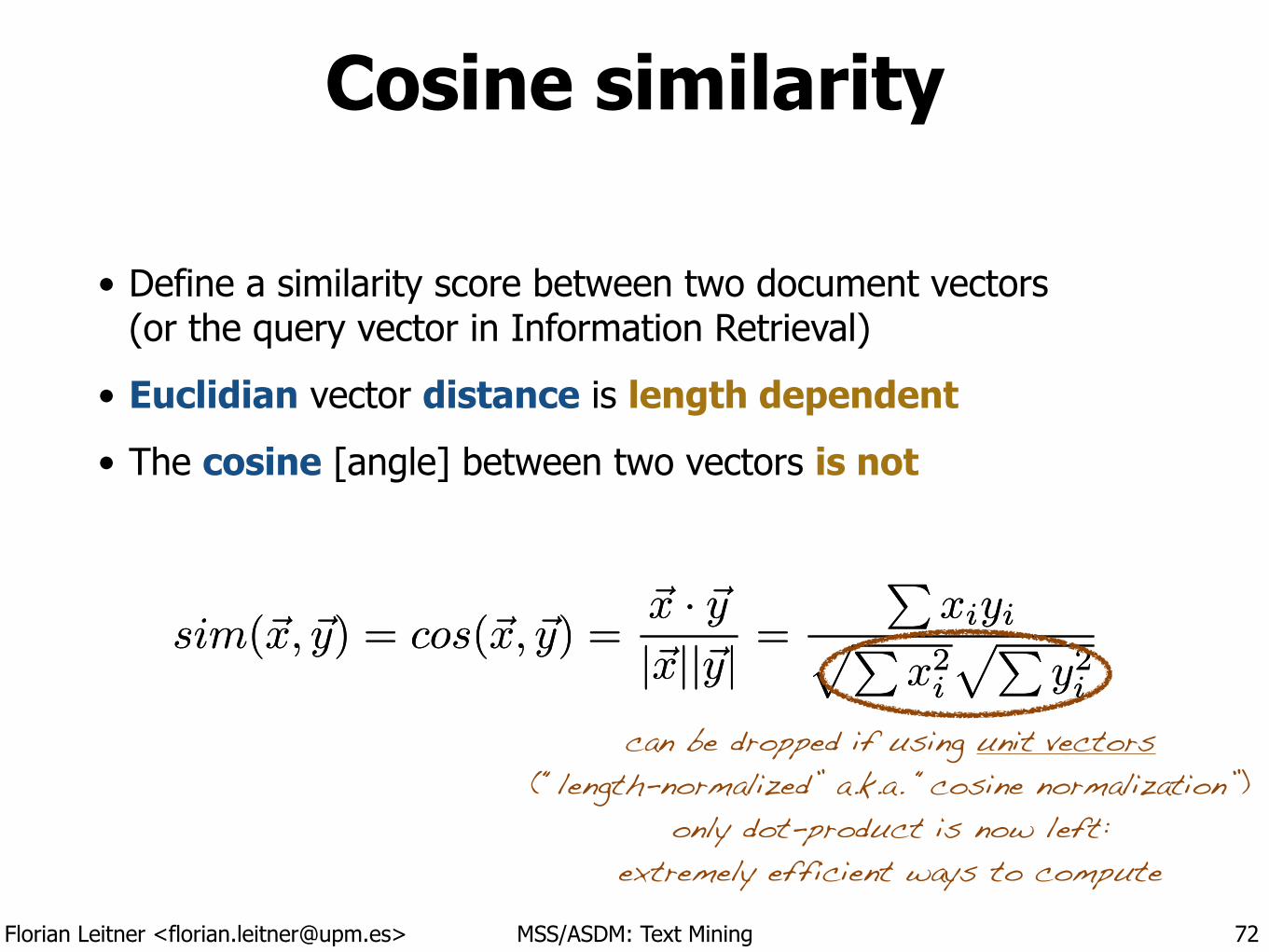
Cosine similarity
• Define a similarity score between two document vectors(or the query vector in Information Retrieval)
• Euclidian vector distance is length dependent
• The cosine [angle] between two vectors is not
72
sim(~x, ~y) = cos(~x, ~y) =~x · ~y|~x||~y| =
PxiyipP
x
2i
pPy
2i
sim(~x, ~y) = cos(~x, ~y) =~x · ~y|~x||~y| =
PxiyipP
x
2i
pPy
2i
can be dropped if using unit vectors (“length-normalized” a.k.a. “cosine normalization”)
only dot-product is now left: extremely efficient ways to compute
Florian Leitner <[email protected]> MSS/ASDM: Text Mining
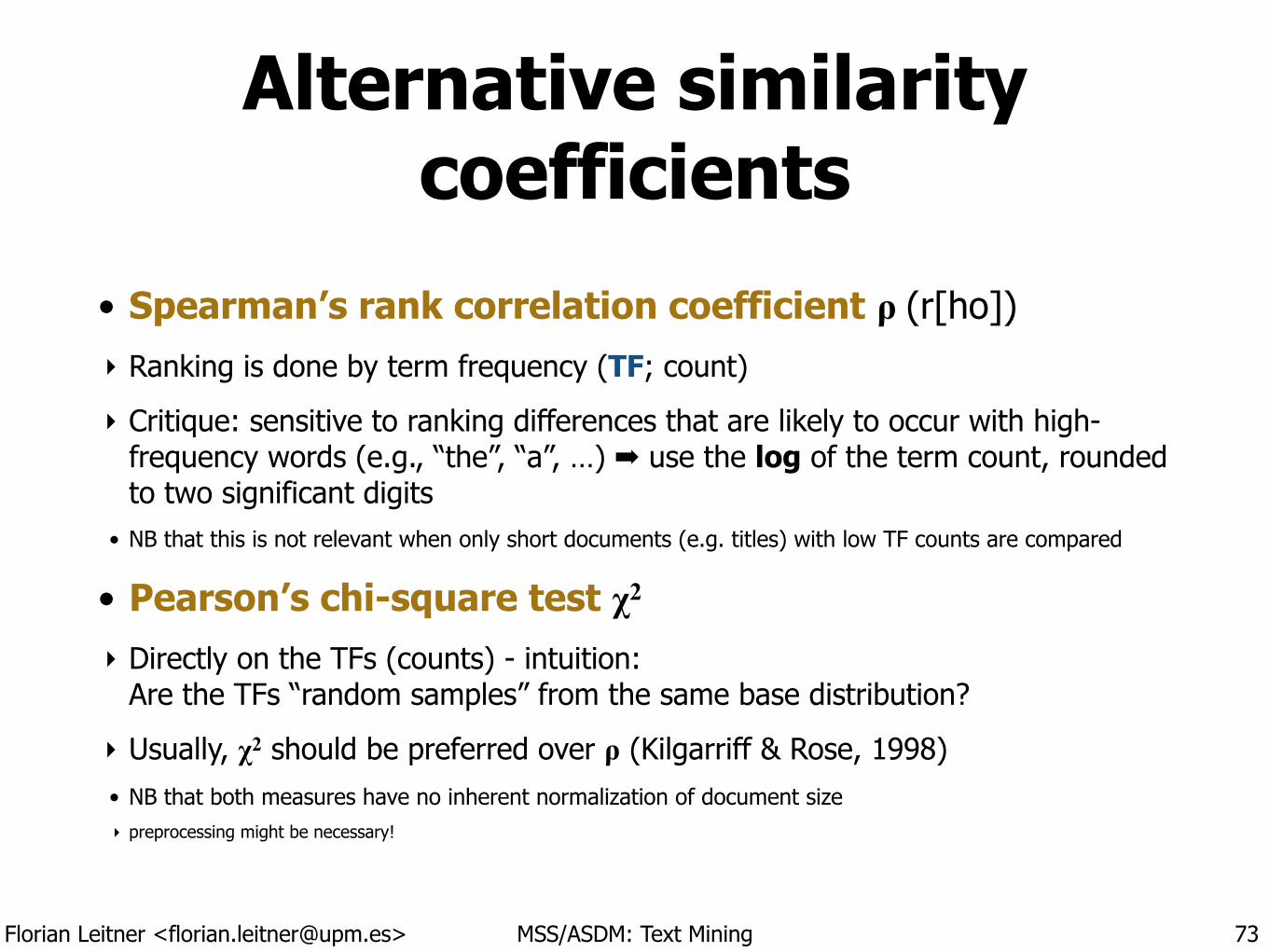
Alternative similarity coefficients
• Spearman’s rank correlation coefficient ρ (r[ho]) ‣ Ranking is done by term frequency (TF; count)
‣ Critique: sensitive to ranking differences that are likely to occur with high-frequency words (e.g., “the”, “a”, …) ➡ use the log of the term count, rounded to two significant digits
• NB that this is not relevant when only short documents (e.g. titles) with low TF counts are compared
• Pearson’s chi-square test χ2 ‣ Directly on the TFs (counts) - intuition:
Are the TFs “random samples” from the same base distribution?
‣ Usually, χ2 should be preferred over ρ (Kilgarriff & Rose, 1998) • NB that both measures have no inherent normalization of document size ‣ preprocessing might be necessary!
73
Florian Leitner <[email protected]> MSS/ASDM: Text Mining
Term Frequency times Inverse Document Frequency (TF-IDF)
• Motivation and background
• The problem ‣ Frequent terms contribute most to a document vector’s direction, but not all
terms are relevant (“the”, “a”, …).
• The goal ‣ Separate important terms from frequent, but irrelevant terms in the
collection.
• The idea ‣ Frequent terms appearing in all documents tend to be less important
versus frequent terms in just a few documents. • Also dampens the effect of topic-specific noun phrases or an author’s bias for a specific set of
adjectives
74
� Zipf’s Law!
Florian Leitner <[email protected]> MSS/ASDM: Text Mining
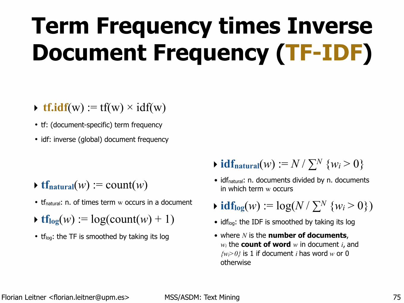
Term Frequency times Inverse Document Frequency (TF-IDF)
‣ tf.idf(w) := tf(w) × idf(w) • tf: (document-specific) term frequency
• idf: inverse (global) document frequency
!!
‣ tfnatural(w) := count(w) • tfnatural: n. of times term w occurs in a document
‣ tflog(w) := log(count(w) + 1) • tflog: the TF is smoothed by taking its log
!
!!!!
‣ idfnatural(w) := N / ∑N {wi > 0} • idfnatural: n. documents divided by n. documents
in which term w occurs
‣ idflog(w) := log(N / ∑N {wi > 0}) • idflog: the IDF is smoothed by taking its log
• where N is the number of documents,wi the count of word w in document i, and {wi>0} is 1 if document i has word w or 0 otherwise
75
Florian Leitner <[email protected]> MSS/ASDM: Text Mining
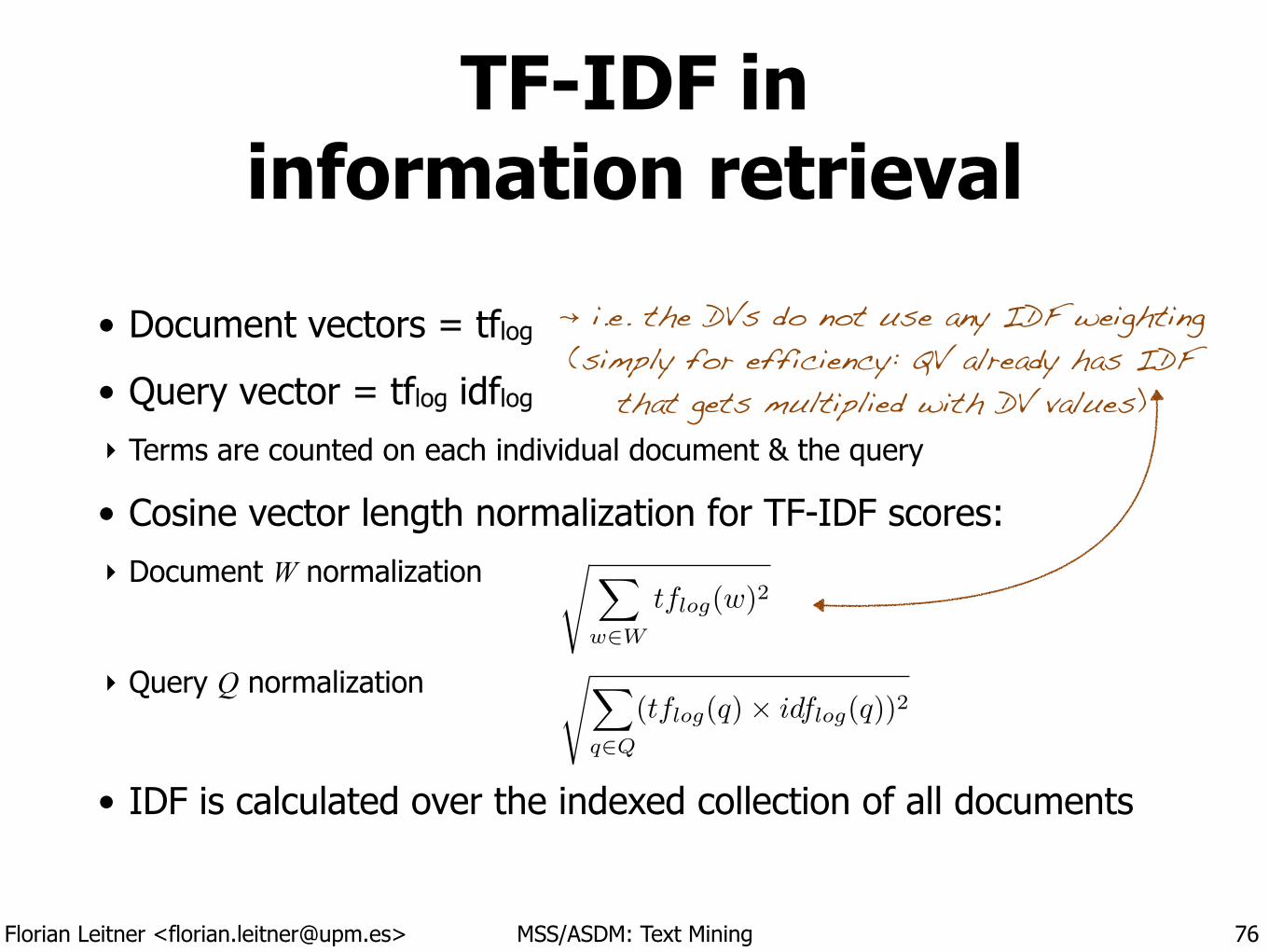
TF-IDF ininformation retrieval
• Document vectors = tflog
• Query vector = tflog idflog
‣ Terms are counted on each individual document & the query
• Cosine vector length normalization for TF-IDF scores: ‣ Document W normalization
!
‣ Query Q normalization
!
• IDF is calculated over the indexed collection of all documents
76
� i.e. the DVs do not use any IDF weighting (simply for efficiency: QV already has IDF
that gets multiplied with DV values)
s X
w2W
tflog
(w)2
sX
q2Q
(tflog
(q)⇥ idflog
(q))2
Florian Leitner <[email protected]> MSS/ASDM: Text Mining
TF-IDF query score: An example
77
Collection Query Q Document D Similarity
Term df idf tf tf tf.idf norm tf tf tf.1 cos(Q,D)
best 3.5E+05 1.46 1 0.30 0.44 0.21 0 0.00 0.00 0.00
text 2.4E+03 3.62 1 0.30 1.09 0.53 10 1.04 0.06 0.03
mining 2.8E+02 4.55 1 0.30 1.37 0.67 8 0.95 0.06 0.04
tutorial 5.5E+03 3.26 1 0.30 0.98 0.48 3 0.60 0.04 0.02
data 9.2E+05 1.04 0 0.00 0.00 0.00 10 1.04 0.06 0.00
… … … … !
… !
0.00 0.00 … !
16.00 … !
0.00
Sums 1.0E+07 4 2.05 ~355 16.11 0.09
3 out of hundreds of unique words match (Jaccard < 0.03)√ of ∑ of 2
Example idea from: Manning et al. Introduction to Information Retrieval. 2009 free PDF!
√ of ∑ of 2 ÷÷
× ×
Florian Leitner <[email protected]> MSS/ASDM: Text Mining
From syntactic to semantic similarity
Cosine Similarity, χ2, Spearman’s ρ, LSH, etc. all compare equal tokens.
But what if you are talking about “automobiles” and I am lazy, calling it a “car”?
We can solve this with Latent Semantic Indexing!
78
Florian Leitner <[email protected]> MSS/ASDM: Text Mining
Latent Semantic Analysis (LSI 1/3)
• a.k.a. Latent Semantic Indexing (in Text Mining): dimensionality reduction for semantic inference
• Linear algebra background ‣ Singular value decomposition of a matrix Q: Q = UΣVT
!
!
!
!
!
• SVD in text mining ‣ Inverted index = doc. eigenvectors × singular values × term eigenvectors
79
singular values:scaling factor
orthonormal factors of Q (QQT and QTQ)
the factors “predict” Q in terms of similarity (Frobeniusnorm) using as many factors as the lower dimension of Q
Q P1 P2 P3G1G2G3G4
P1 P2 P3PlayersU
G1G2G3G4
 ’ Â’’
Game
s
avrg g
ame
scor
e
player abilityavr
g sco
re
delta
s
player ability deltas
= ×S
SS
scaling factors !!!!
(U and V are eigenvectors)
×
Florian Leitner <[email protected]> MSS/ASDM: Text Mining
Latent Semantic Analysis (LSI 2/3)
• Image taken from: Manning et al. An Introduction to IR. 2009
80
‣ Inverted index = doc. eigenvectors × singular values × term eigenvectors
docs
terms
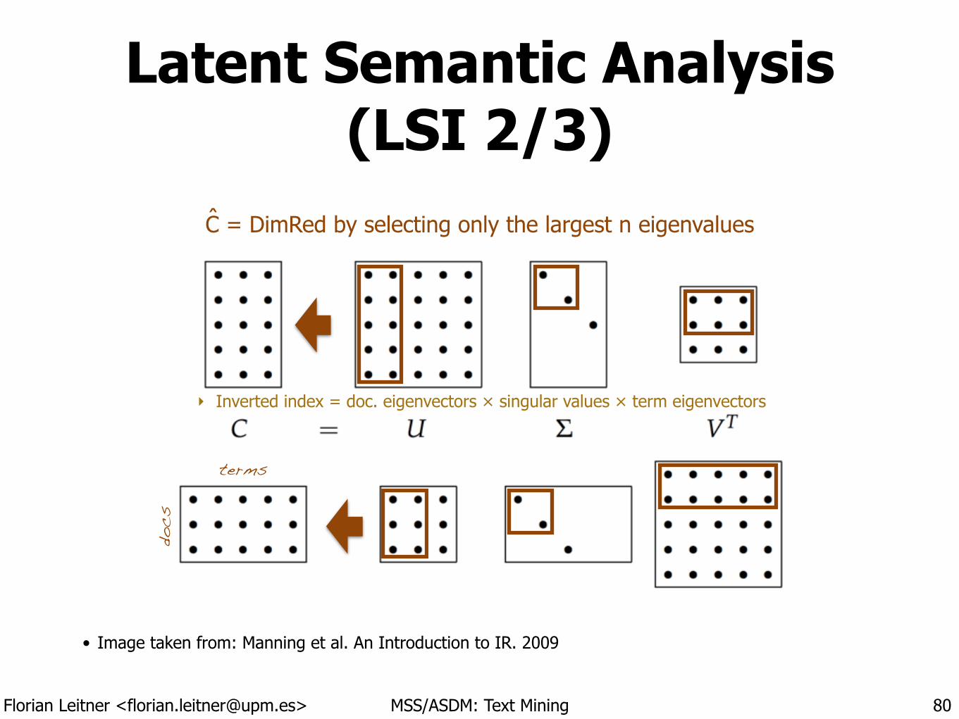
Florian Leitner <[email protected]> MSS/ASDM: Text Mining
Latent Semantic Analysis (LSI 2/3)
• Image taken from: Manning et al. An Introduction to IR. 2009
80
‣ Inverted index = doc. eigenvectors × singular values × term eigenvectors
docs
terms
C = DimRed by selecting only the largest n eigenvaluesˆ
Florian Leitner <[email protected]> MSS/ASDM: Text Mining
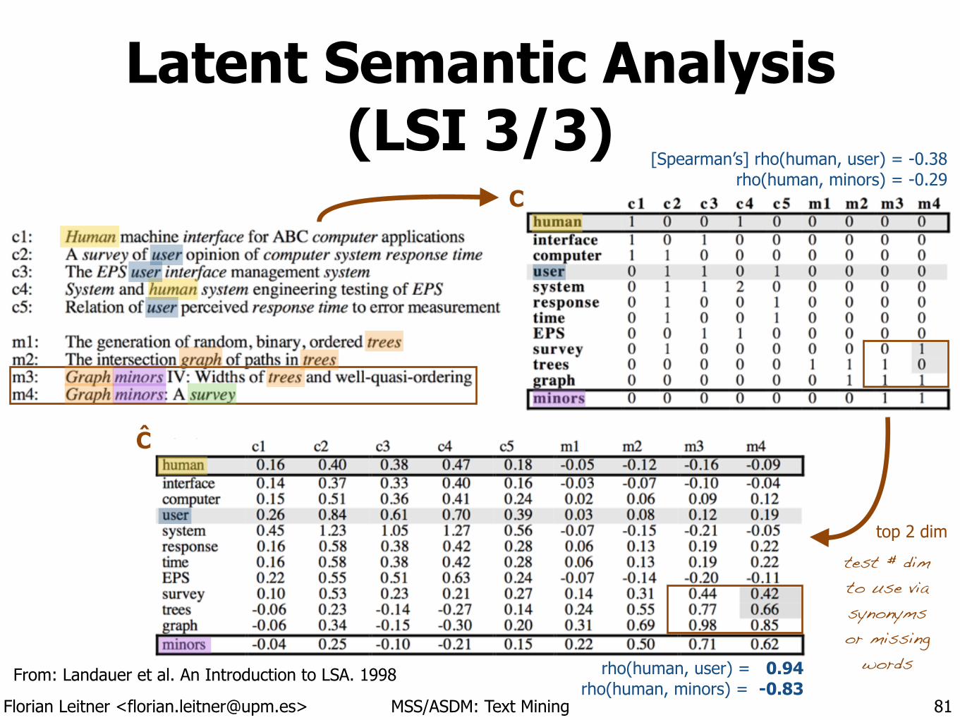
Latent Semantic Analysis (LSI 3/3)
81
From: Landauer et al. An Introduction to LSA. 1998
C
C
top 2 dim
[Spearman’s] rho(human, user) = -0.38 rho(human, minors) = -0.29
rho(human, user) = 0.94 rho(human, minors) = -0.83
test # dim to use via synonyms or missing
words
Florian Leitner <[email protected]> MSS/ASDM: Text Mining
Principal Component vs. Latent Semantic Analysis
• LSA seeks for the best linear subspace in Frobenius norm, while PCA aims for the best affine linear subspace.
• LSA (can) use TF-IDF weighting as preprocessing step.
• PCA requires the (square) covariance matrix of the original matrix as its first step and therefore can only compute term-term or doc-doc similarities.
• PCA matrices are more dense (zeros occur only when true independence is detected).
82
best Frobenius norm: minimize “std. dev.” of matrix best affine subspace: minimize dimensions while maintaing the form
Florian Leitner <[email protected]> MSS/ASDM: Text Mining
From similarity to labels
• So far, we have seen how to establish if two documents are syntactically (kNN/LSH) and even semantically (LSI) similar.
!
• But how do we now assign a label (a “class”) to a document? ‣ E.g., relevant/not relevant; polarity (positive, neutral, negative);
a topic (politics, sport, people, science, healthcare, …)
‣ We could use the distances (e.g., from LSI) to cluster the documents
‣ Instead, let’s look at supervised methods next.
83
Florian Leitner <[email protected]> MSS/ASDM: Text Mining
Text classification approaches
• Multinomial naïve Bayes*
• Nearest neighbor classification (ASDM Course) ‣ incl. locality sensitivity hashing* (already seen)
• Latent semantic indexing* (already seen)
• Cluster analysis (ASDM Course)
• Maximum entropy classification*
• Latent Dirichlet allocation*
• Random forests
• Support vector machines (ASDM Course)
• Artificial neural networks (ASDM Course)
84
effic
ient/
fast
tra
ining
high
acc
urac
y
* this course
Florian Leitner <[email protected]> MSS/ASDM: Text Mining
Three text classifiers
• Multinomial naïve Bayes
• Maximum entropy (multinomial logistic regression)
• Latent Dirichlet allocation unsupervised!
85
Florian Leitner <[email protected]> MSS/ASDM: Text Mining
Maximum A Posterior (MAP) estimator
• Issue: Predict the class c ∈ C for a given document d ∈ D
• Solution: MAP, a “perfect” Bayesian estimator:
!
!
!
• Problem: d is really the set {w1, …, wn} of dependent words W ‣ exponential parameterization: one for each possible combination of W and C
86
CMAP (d) = argmax
c2CP (c|d) = argmax
c2C
P (d|c)P (c)
P (d)redundantthe posterior
Florian Leitner <[email protected]> MSS/ASDM: Text Mining
Multinomial naïve Bayes classification
• A simplification of the MAP Estimator ‣ count(w) is a discrete, multinomial variable (unigrams, bigrams, etc.)
‣ Reduce space by making a strong independence assumption (“naïve”)
!
!
• Easy parameter estimation !
!
‣ V is the entire vocabulary (collection of unique words/n-grams/…) in D
‣ uses Laplacian/add-one smoothing
87
independence assumption: “each word is on its own”
“bag of words/features”
P (wi|c) =count(wi, c) + 1
|V |+P
w2V count(w, c)
CMAP (d) = argmax
c2CP (d|c)P (c) ⇡ argmax
c2CP (c)
Y
w2W
P (w|c)
count(wi, c): the total count of word i in all documents of class c [in our training set]
Florian Leitner <[email protected]> MSS/ASDM: Text Mining
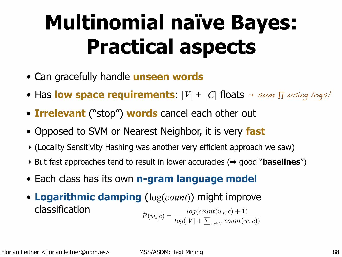
Multinomial naïve Bayes: Practical aspects
• Can gracefully handle unseen words
• Has low space requirements: |V| + |C| floats
• Irrelevant (“stop”) words cancel each other out
• Opposed to SVM or Nearest Neighbor, it is very fast ‣ (Locality Sensitivity Hashing was another very efficient approach we saw)
‣ But fast approaches tend to result in lower accuracies (➡ good “baselines”)
• Each class has its own n-gram language model
• Logarithmic damping (log(count)) might improve classification
88
� sum ∏ using logs!
P (wi|c) =log(count(wi, c) + 1)
log(|V |+P
w2V count(w, c))
Text Mining 4 Text Classification
!Madrid Summer School on
Advanced Statistics and Data Mining !
Florian Leitner [email protected]
License:
Florian Leitner <[email protected]> MSS/ASDM: Text Mining
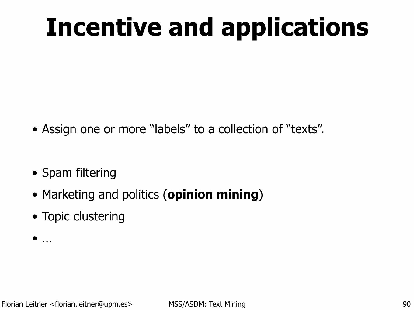
Incentive and applications
• Assign one or more “labels” to a collection of “texts”.
!
• Spam filtering
• Marketing and politics (opinion mining)
• Topic clustering
• …
90
Florian Leitner <[email protected]> MSS/ASDM: Text Mining
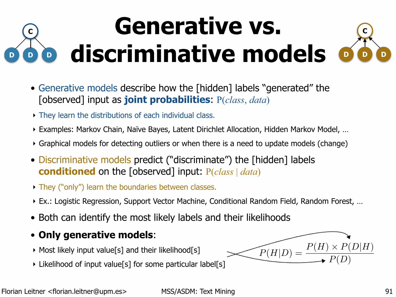
Generative vs. discriminative models
• Generative models describe how the [hidden] labels “generated” the [observed] input as joint probabilities: P(class, data)
‣ They learn the distributions of each individual class.
‣ Examples: Markov Chain, Naïve Bayes, Latent Dirichlet Allocation, Hidden Markov Model, …
‣ Graphical models for detecting outliers or when there is a need to update models (change)
• Discriminative models predict (“discriminate”) the [hidden] labels conditioned on the [observed] input: P(class | data)
‣ They (“only”) learn the boundaries between classes.
‣ Ex.: Logistic Regression, Support Vector Machine, Conditional Random Field, Random Forest, …
• Both can identify the most likely labels and their likelihoods
• Only generative models: ‣ Most likely input value[s] and their likelihood[s]
‣ Likelihood of input value[s] for some particular label[s]
91
D D
C
D D D
C
D
P (H|D) =P (H)⇥ P (D|H)
P (D)
Florian Leitner <[email protected]> MSS/ASDM: Text Mining
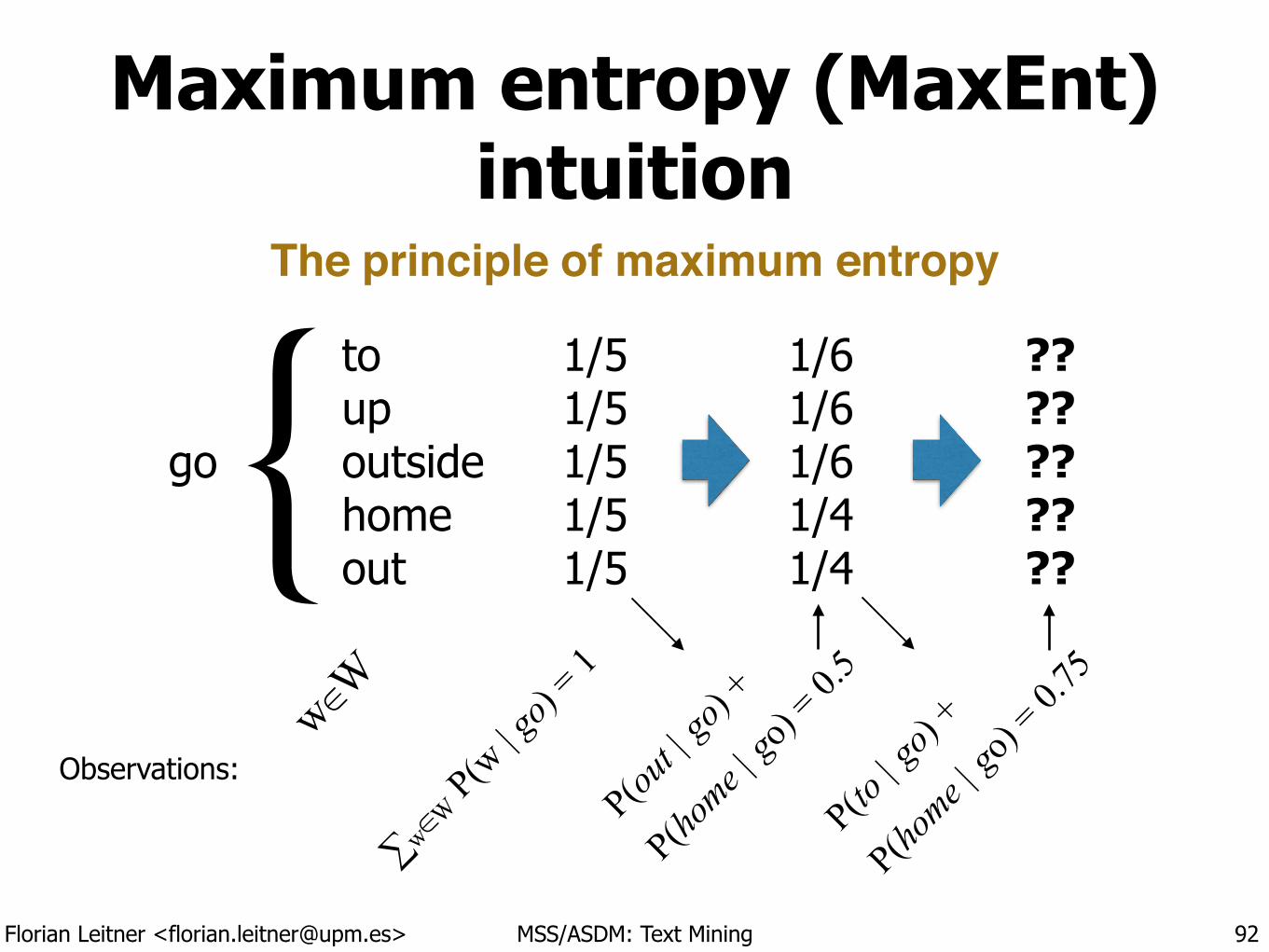
Maximum entropy (MaxEnt) intuition
92
go
to up outside home out
{w∈
W
∑w∈W P(w
| go)
= 1
1/5 1/5 1/5 1/5 1/5
The principle of maximum entropy
Observations:
1/6 1/6 1/6 1/4 1/4
P(out |
go) +
P(home |
go) =
0.5
?? ?? ?? ?? ??
P(to | g
o) +
P(home |
go) =
0.75
Florian Leitner <[email protected]> MSS/ASDM: Text Mining
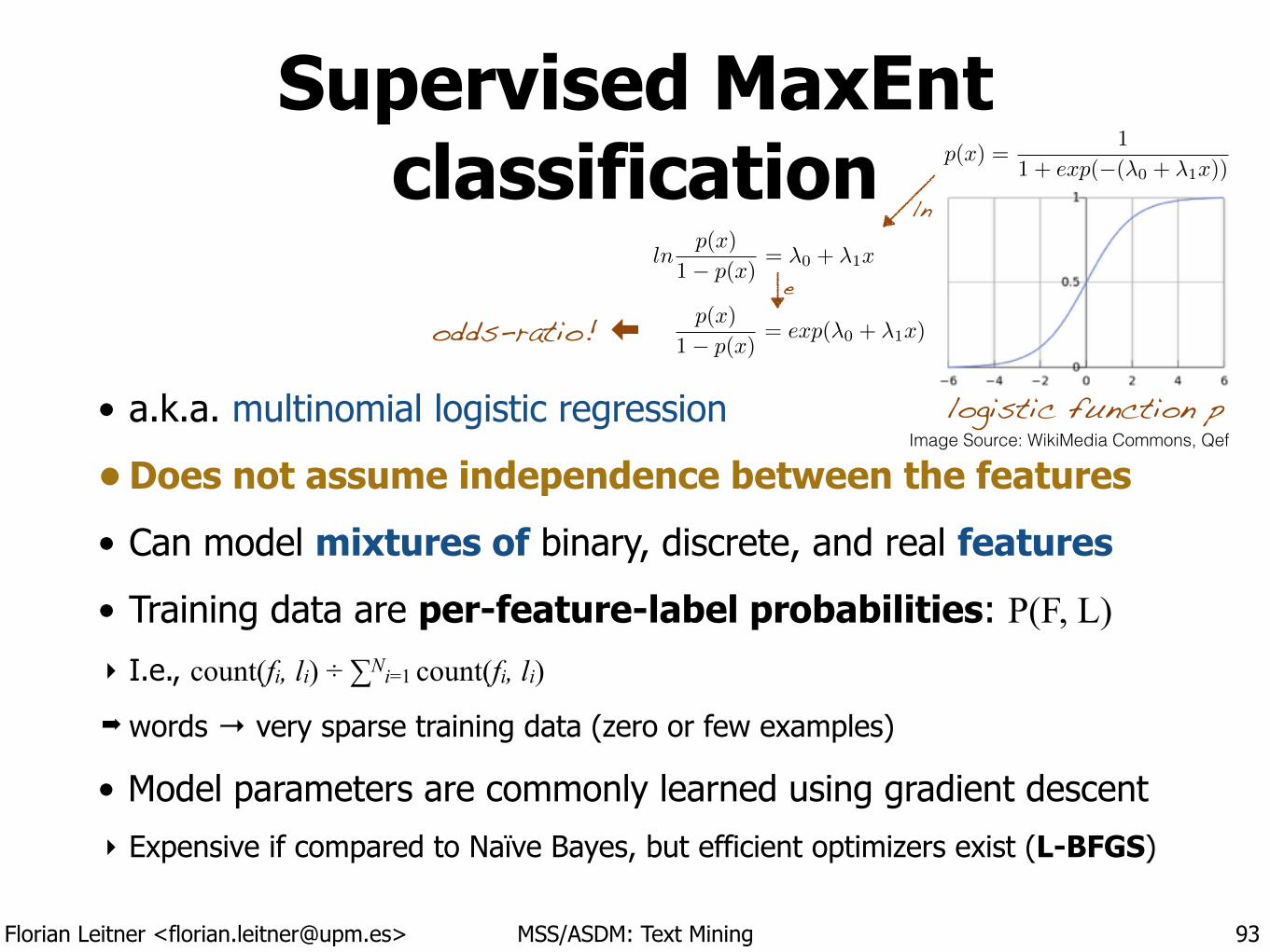
Supervised MaxEnt classification
• a.k.a. multinomial logistic regression
• Does not assume independence between the features
• Can model mixtures of binary, discrete, and real features
• Training data are per-feature-label probabilities: P(F, L) ‣ I.e., count(fi, li) ÷ ∑Ni=1 count(fi, li)
➡ words → very sparse training data (zero or few examples)
• Model parameters are commonly learned using gradient descent ‣ Expensive if compared to Naïve Bayes, but efficient optimizers exist (L-BFGS)
93
logistic function p
p(x) =1
1 + exp(�(�0 + �1x))
ln
p(x)
1� p(x)= �0 + �1x
p(x)
1� p(x)= exp(�0 + �1x)odds-ratio! ⬅
ln
e
Image Source: WikiMedia Commons, Qef
Florian Leitner <[email protected]> MSS/ASDM: Text Mining
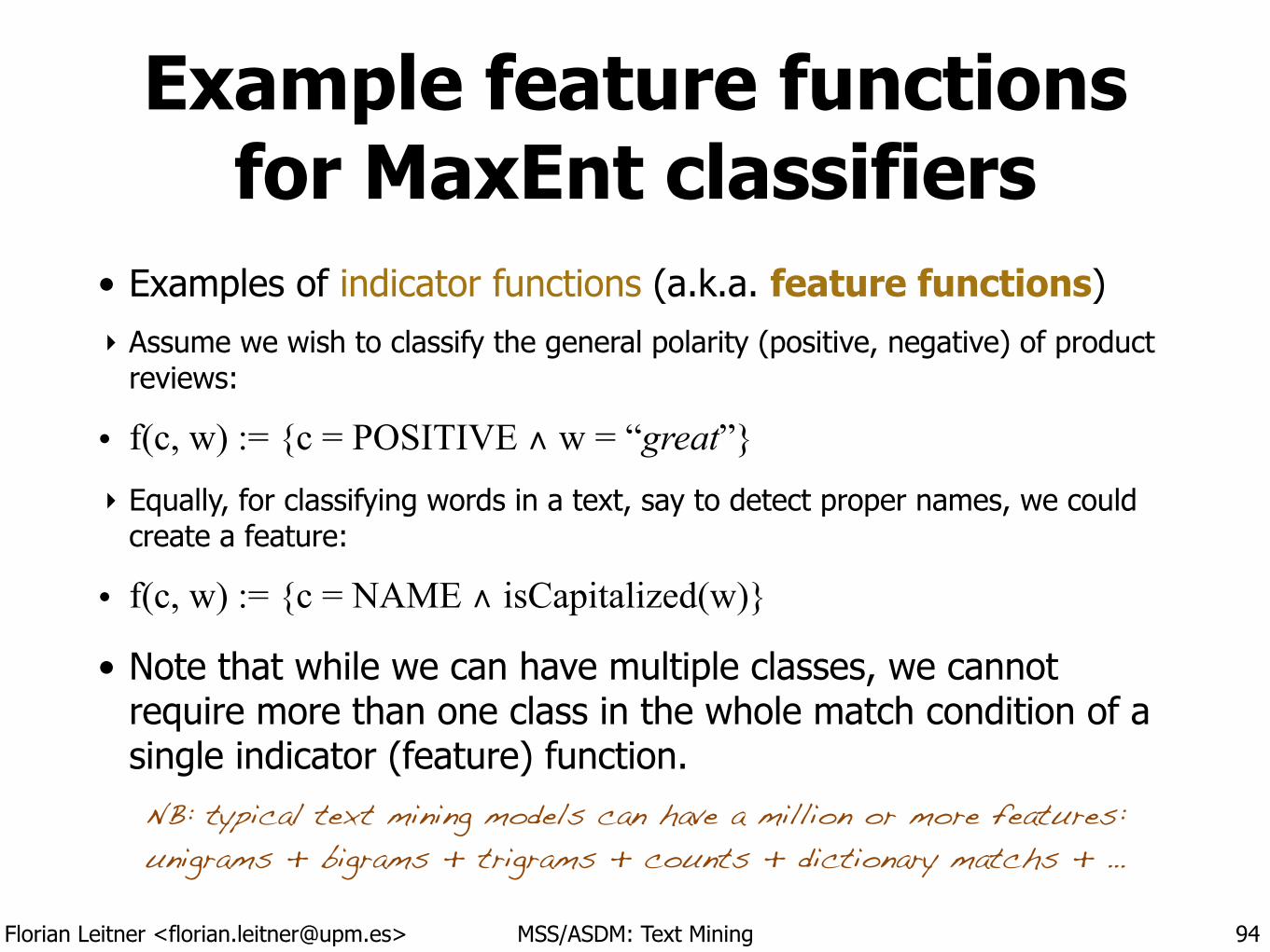
Example feature functions for MaxEnt classifiers
• Examples of indicator functions (a.k.a. feature functions) ‣ Assume we wish to classify the general polarity (positive, negative) of product
reviews:
• f(c, w) := {c = POSITIVE ∧ w = “great”} ‣ Equally, for classifying words in a text, say to detect proper names, we could
create a feature:
• f(c, w) := {c = NAME ∧ isCapitalized(w)}
• Note that while we can have multiple classes, we cannot require more than one class in the whole match condition of a single indicator (feature) function.
94
NB: typical text mining models can have a million or more features: unigrams + bigrams + trigrams + counts + dictionary matchs + …
Florian Leitner <[email protected]> MSS/ASDM: Text Mining
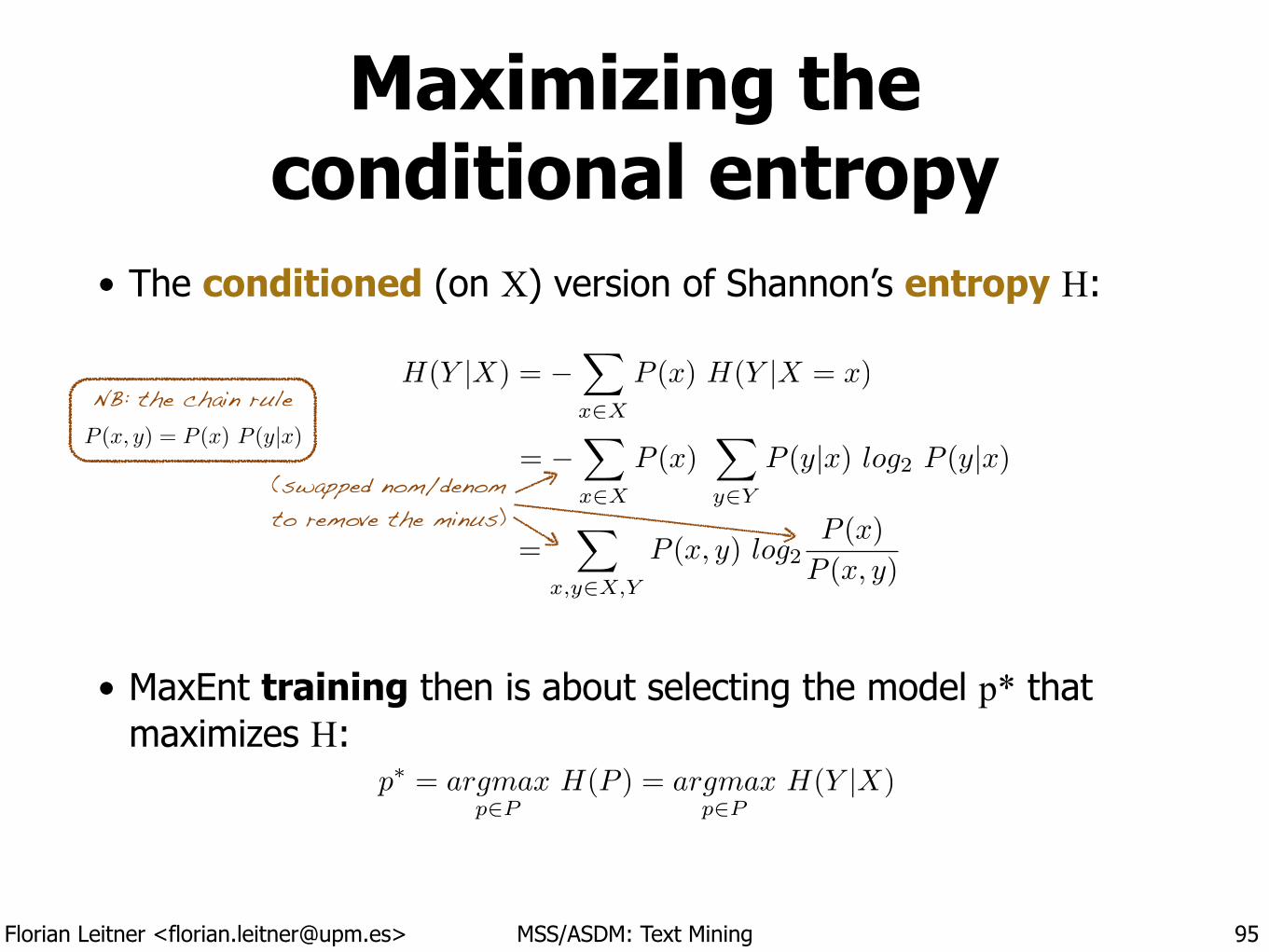
Maximizing theconditional entropy
• The conditioned (on X) version of Shannon’s entropy H:
!
!
!
!
!
• MaxEnt training then is about selecting the model p* that maximizes H:
95
H(Y |X) = �X
x2X
P (x) H(Y |X = x)
= �X
x2X
P (x)X
y2Y
P (y|x) log2 P (y|x)
=X
x,y2X,Y
P (x, y) log2P (x)
P (x, y)
(swapped nom/denom to remove the minus)
p⇤ = argmaxp2P
H(P ) = argmaxp2P
H(Y |X)
P (x, y) = P (x) P (y|x)NB: the chain rule
Florian Leitner <[email protected]> MSS/ASDM: Text Mining
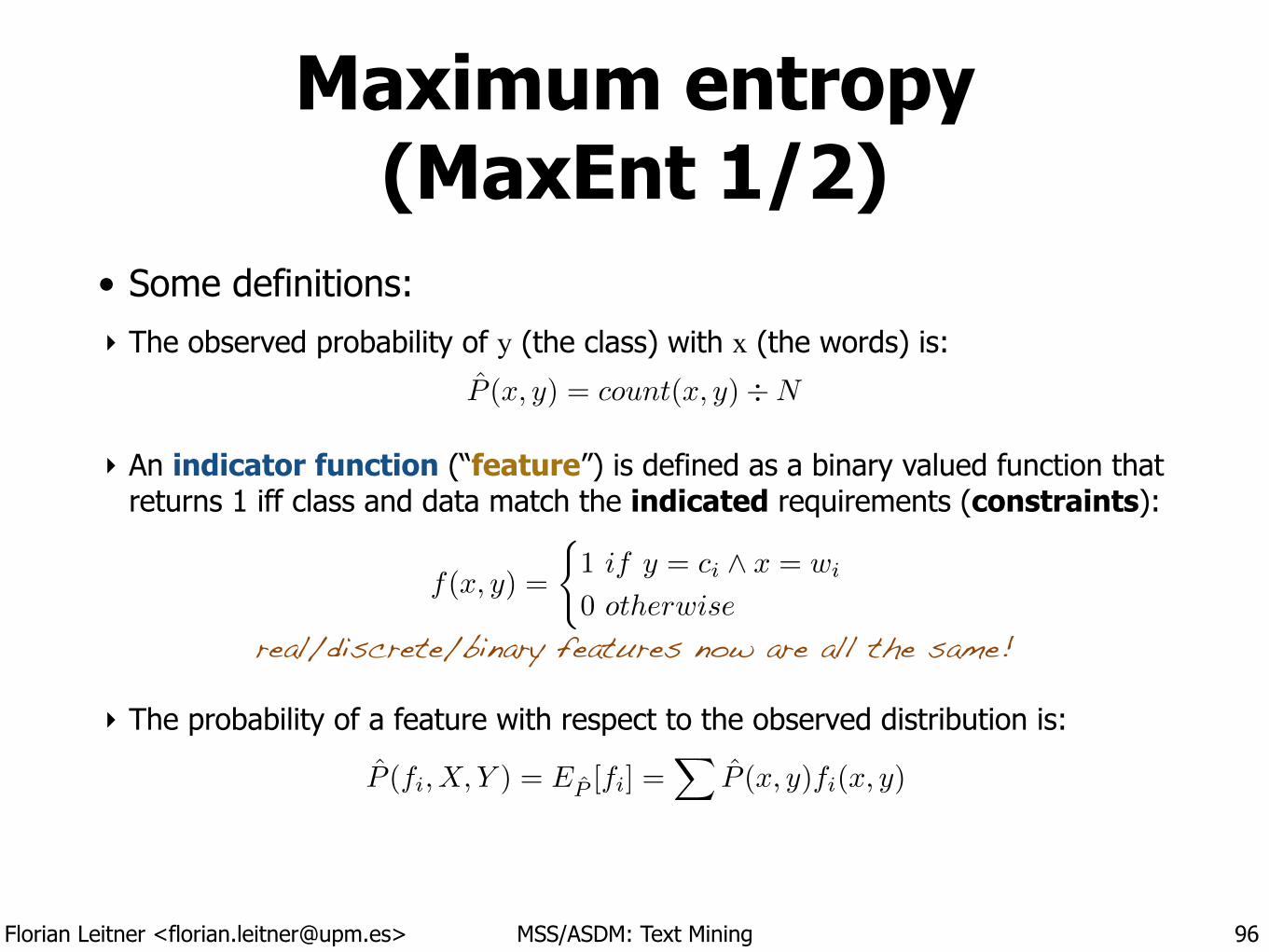
Maximum entropy (MaxEnt 1/2)
• Some definitions: ‣ The observed probability of y (the class) with x (the words) is:
!
‣ An indicator function (“feature”) is defined as a binary valued function that returns 1 iff class and data match the indicated requirements (constraints):
!
!
!
‣ The probability of a feature with respect to the observed distribution is:
96
f(x, y) =
(1 if y = ci ^ x = wi
0 otherwise
P (x, y) = count(x, y)÷N
P (fi, X, Y ) = EP [fi] =X
P (x, y)fi(x, y)
real/discrete/binary features now are all the same!
Florian Leitner <[email protected]> MSS/ASDM: Text Mining
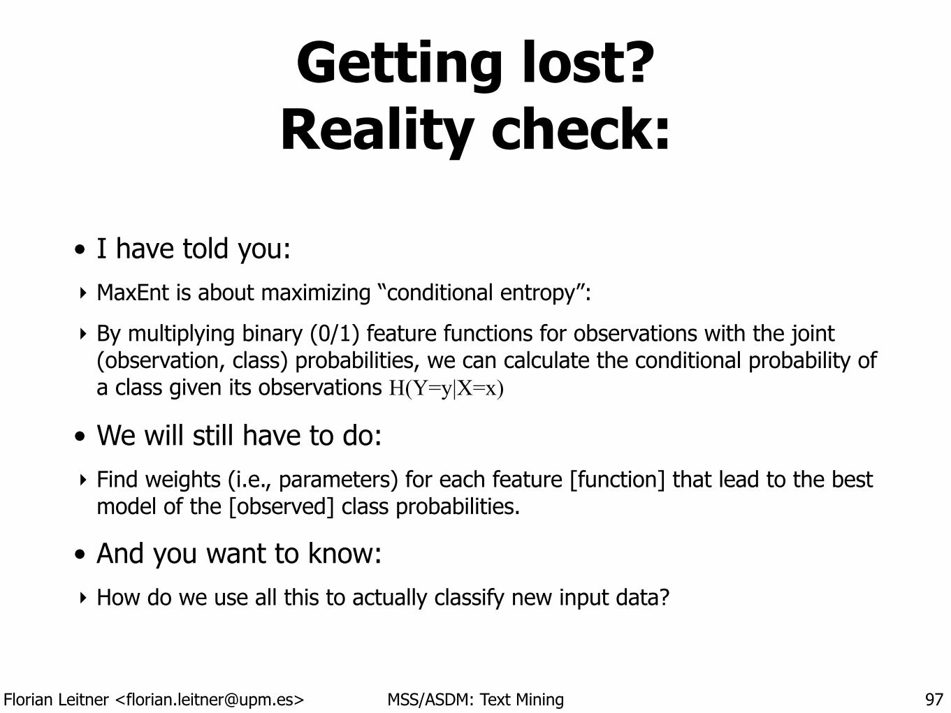
Getting lost? Reality check:
• I have told you: ‣ MaxEnt is about maximizing “conditional entropy”:
‣ By multiplying binary (0/1) feature functions for observations with the joint (observation, class) probabilities, we can calculate the conditional probability of a class given its observations H(Y=y|X=x)
• We will still have to do: ‣ Find weights (i.e., parameters) for each feature [function] that lead to the best
model of the [observed] class probabilities.
• And you want to know: ‣ How do we use all this to actually classify new input data?
97
Florian Leitner <[email protected]> MSS/ASDM: Text Mining
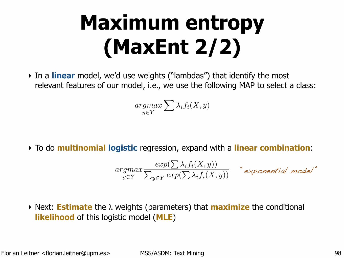
Maximum entropy (MaxEnt 2/2)
‣ In a linear model, we’d use weights (“lambdas”) that identify the most relevant features of our model, i.e., we use the following MAP to select a class:
!
!
!
‣ To do multinomial logistic regression, expand with a linear combination:
!
!
!
‣ Next: Estimate the λ weights (parameters) that maximize the conditional likelihood of this logistic model (MLE)
98
“exponential model”argmax
y2Y
exp(P
�ifi(X, y))Py2Y exp(
P�ifi(X, y))
argmax
y2Y
X�ifi(X, y)
Florian Leitner <[email protected]> MSS/ASDM: Text Mining
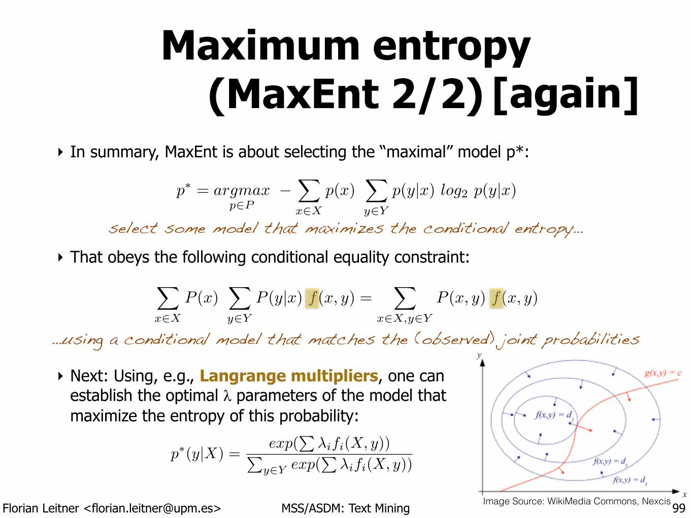
Maximum entropy (MaxEnt 2/2)
‣ In summary, MaxEnt is about selecting the “maximal” model p*: !!!
‣ That obeys the following conditional equality constraint:
!
!
!
‣ Next: Using, e.g., Langrange multipliers, one canestablish the optimal λ parameters of the model that maximize the entropy of this probability:
99
X
x2X
P (x)X
y2Y
P (y|x) f(x, y) =X
x2X,y2Y
P (x, y) f(x, y)
p
⇤ = argmax
p2P
�X
x2X
p(x)X
y2Y
p(y|x) log2 p(y|x)
…using a conditional model that matches the (observed) joint probabilities
select some model that maximizes the conditional entropy…
[again]
Image Source: WikiMedia Commons, Nexcis
p
⇤(y|X) =exp(
P�ifi(X, y))P
y2Y exp(P
�ifi(X, y))
Florian Leitner <[email protected]> MSS/ASDM: Text Mining
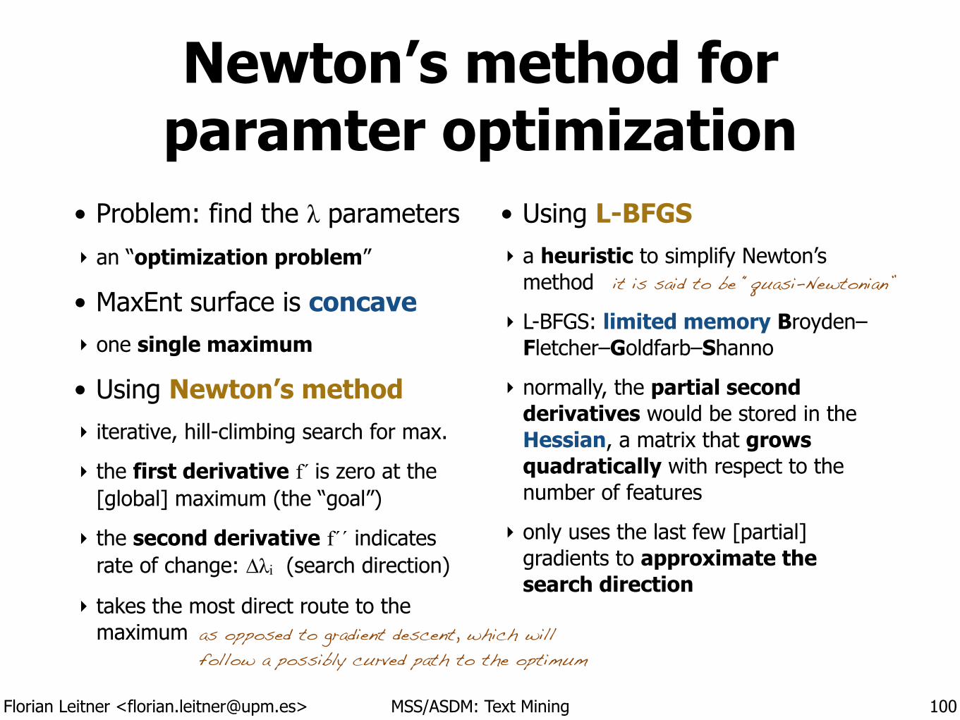
Newton’s method for paramter optimization
• Problem: find the λ parameters
‣ an “optimization problem”
• MaxEnt surface is concave ‣ one single maximum
• Using Newton’s method ‣ iterative, hill-climbing search for max.
‣ the first derivative f´ is zero at the [global] maximum (the “goal”)
‣ the second derivative f´´ indicates rate of change: ∆λi (search direction)
‣ takes the most direct route to the maximum
• Using L-BFGS ‣ a heuristic to simplify Newton’s
method
‣ L-BFGS: limited memory Broyden–Fletcher–Goldfarb–Shanno
‣ normally, the partial second derivatives would be stored in the Hessian, a matrix that grows quadratically with respect to the number of features
‣ only uses the last few [partial] gradients to approximate the search direction
100
it is said to be “quasi-Newtonian”
as opposed to gradient descent, which will follow a possibly curved path to the optimum
Florian Leitner <[email protected]> MSS/ASDM: Text Mining
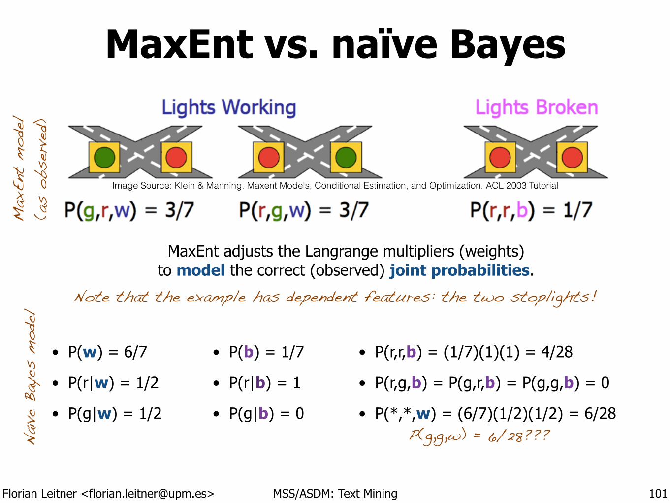
MaxEnt vs. naïve Bayes
• P(w) = 6/7
• P(r|w) = 1/2
• P(g|w) = 1/2
101
Note that the example has dependent features: the two stoplights!
Max
Ent
mode
l (a
s ob
serve
d)Na
ïve B
ayes
mod
el
MaxEnt adjusts the Langrange multipliers (weights) to model the correct (observed) joint probabilities.
• P(r,r,b) = (1/7)(1)(1) = 4/28
• P(r,g,b) = P(g,r,b) = P(g,g,b) = 0
• P(*,*,w) = (6/7)(1/2)(1/2) = 6/28
• P(b) = 1/7
• P(r|b) = 1
• P(g|b) = 0P(g,g,w) = 6/28???
Image Source: Klein & Manning. Maxent Models, Conditional Estimation, and Optimization. ACL 2003 Tutorial
Florian Leitner <[email protected]> MSS/ASDM: Text Mining
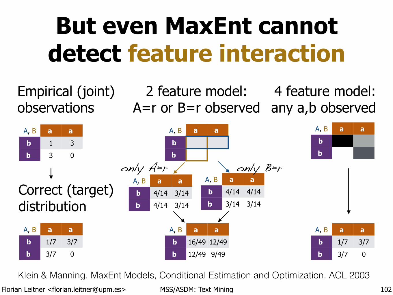
But even MaxEnt cannot detect feature interaction
102
A, B a a
b 1 3
b 3 0
Klein & Manning. MaxEnt Models, Conditional Estimation and Optimization. ACL 2003
Empirical (joint) observations
Correct (target) distribution
A, B a a
b 1/7 3/7
b 3/7 0
2 feature model: A=r or B=r observed
A, B a a
b 16/49 12/49
b 12/49 9/49
A, B a a
b
b
4 feature model: any a,b observed
A, B a a
b 1/7 3/7
b 3/7 0
A, B a a
b
b
A, B a a
b 4/14 3/14
b 4/14 3/14
A, B a a
b 4/14 4/14
b 3/14 3/14
only A=r only B=r
Florian Leitner <[email protected]> MSS/ASDM: Text Mining
A first look at probabilistic graphical models
• Latent Dirichlet Allocation: LDA ‣ Blei, Ng, and Jordan. Journal of Machine Learning Research 2003
‣ For assigning “topics” to “documents”
‣ An unsupervised, generative model
103
i.e., for text classification
Florian Leitner <[email protected]> MSS/ASDM: Text Mining
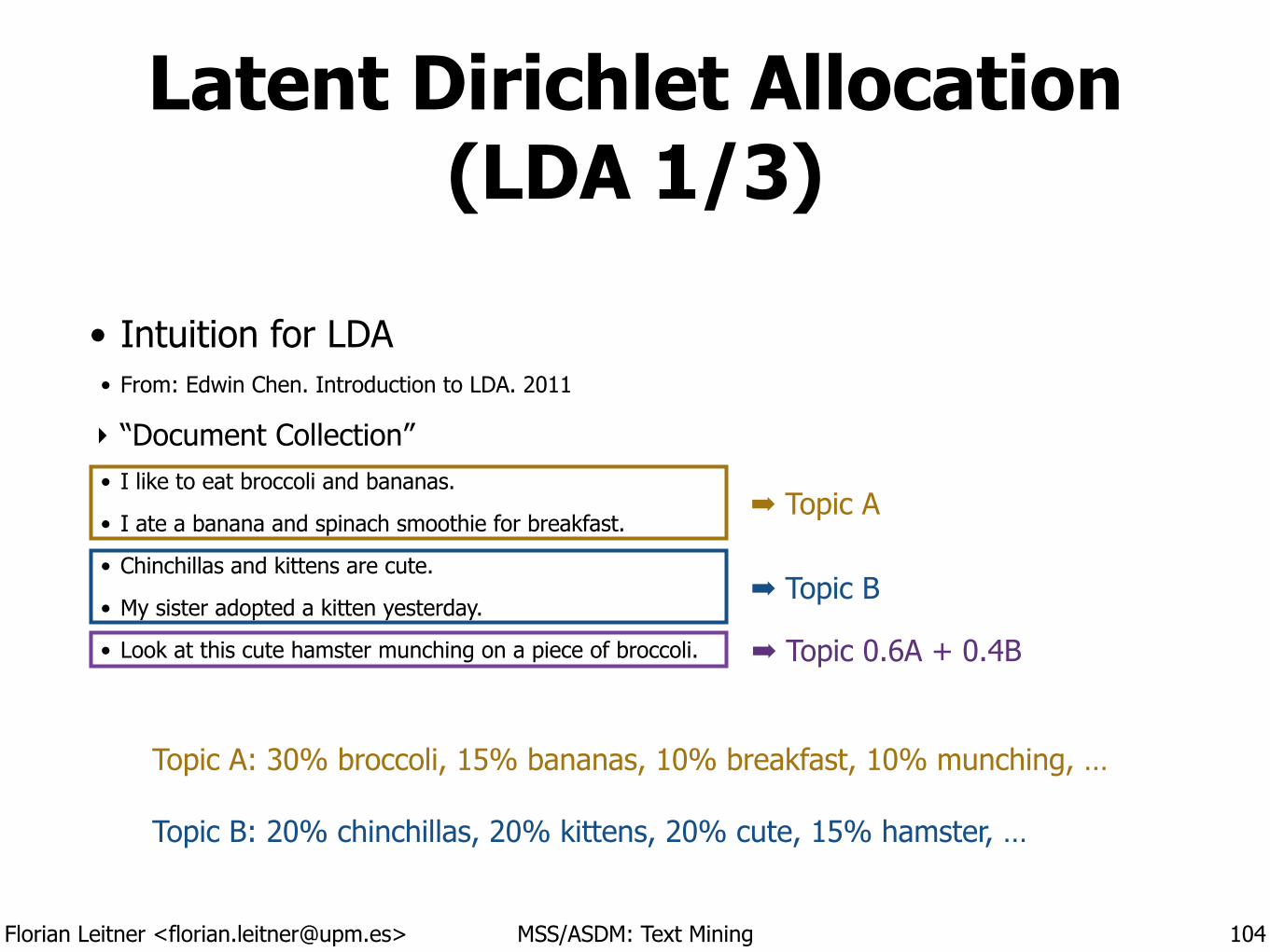
Latent Dirichlet Allocation (LDA 1/3)
• Intuition for LDA • From: Edwin Chen. Introduction to LDA. 2011
‣ “Document Collection” • I like to eat broccoli and bananas.
• I ate a banana and spinach smoothie for breakfast.
• Chinchillas and kittens are cute.
• My sister adopted a kitten yesterday.
• Look at this cute hamster munching on a piece of broccoli.
!!
104
➡ Topic A
➡ Topic B
➡ Topic 0.6A + 0.4B
Topic A: 30% broccoli, 15% bananas, 10% breakfast, 10% munching, … !Topic B: 20% chinchillas, 20% kittens, 20% cute, 15% hamster, …
Florian Leitner <[email protected]> MSS/ASDM: Text Mining
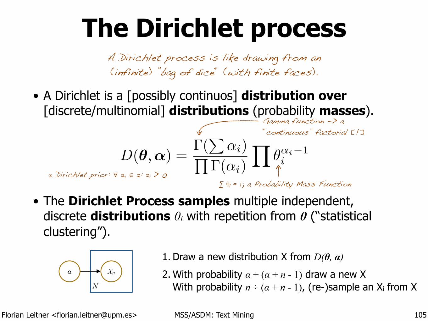
The Dirichlet process
• A Dirichlet is a [possibly continuos] distribution over [discrete/multinomial] distributions (probability masses).
!
!
!
• The Dirichlet Process samples multiple independent, discrete distributions θi with repetition from θ (“statistical clustering”).
105
D(✓,↵) =�(
P↵i)Q
�(↵i)
Y✓↵i�1i
Xnα
N
A Dirichlet process is like drawing from an (infinite) ”bag of dice“ (with finite faces).
1. Draw a new distribution X from D(θ, α)
2. With probability α ÷ (α + n - 1) draw a new XWith probability n ÷ (α + n - 1), (re-)sample an Xi from X
∑ �i = 1; a Probability Mass Function
Gamma function -> a “continuous” factorial [!]
� Dirichlet prior: ∀ �i ∈ �: �i > 0
Florian Leitner <[email protected]> MSS/ASDM: Text Mining
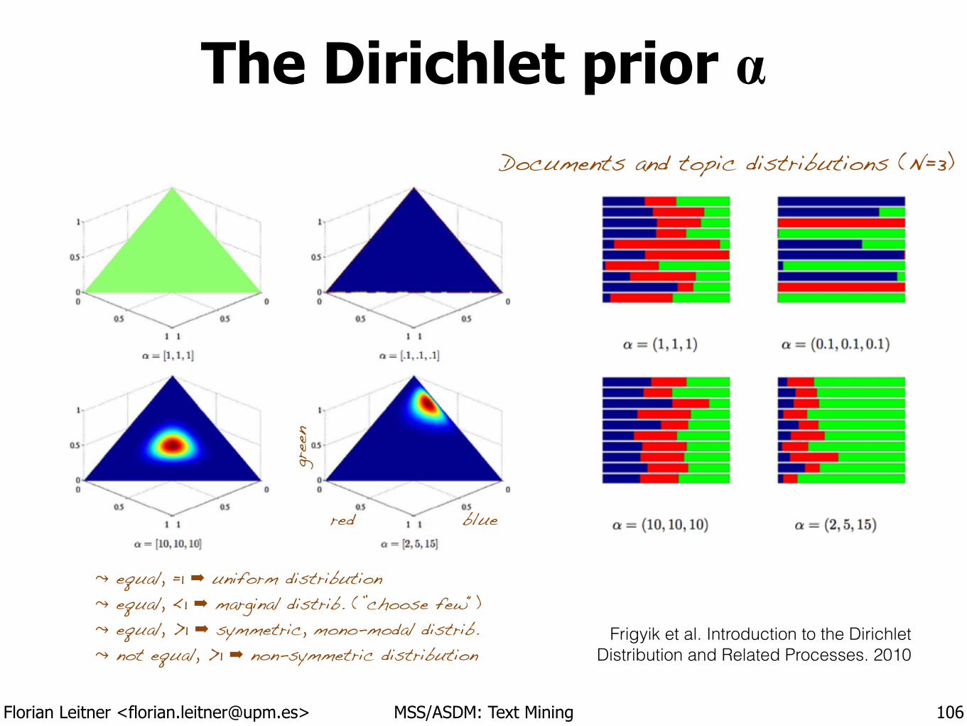
The Dirichlet prior α
106
bluered
gree
n
Frigyik et al. Introduction to the Dirichlet Distribution and Related Processes. 2010
⤳ equal, =1 ➡ uniform distribution ⤳ equal, <1 ➡ marginal distrib. (”choose few“) ⤳ equal, >1 ➡ symmetric, mono-modal distrib. ⤳ not equal, >1 ➡ non-symmetric distribution
Documents and topic distributions (N=3)
Florian Leitner <[email protected]> MSS/ASDM: Text Mining
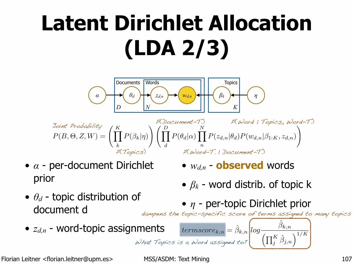
Latent Dirichlet Allocation (LDA 2/3)
• α - per-document Dirichlet prior
• θd - topic distribution of document d
• zd,n - word-topic assignments
• wd,n - observed words
• βk - word distrib. of topic k
• η - per-topic Dirichlet prior
107
βkwd,nzd,nθdα η
ND K
Documents Words Topics
P (B,⇥, Z,W ) =
KY
k
P (�k|⌘)!
DY
d
P (✓d|↵)NY
n
P (zd,n|✓d)P (wd,n|�1:K , zd,n)
!
P(Topics)
P(Document-T.)
P(Word-T. | Document-T.)
P(Word | Topics, Word-T.)Joint Probability
termscorek,n = �k,n log
�k,n⇣QK
j �j,n
⌘1/K
dampens the topic-specific score of terms assigned to many topics
What Topics is a Word assigned to?
Florian Leitner <[email protected]> MSS/ASDM: Text Mining
Latent Dirichlet Allocation (LDA 3/3)
• LDA inference in a nutshell ‣ Calculate the posterior probability that Topic t generated Word w.
‣ Initialization: Choose K, the number of Topics, and randomly assign one out of the K Topics to each of the N Words in each of the D Documents.
• The same word can have different Topics at different positions in the Document.
‣ Then, for each Topic:And for each Word in each Document:
1. Compute P(Word-Topic | Document): the proportion of [Words assigned to] Topic t in Document d
2. Compute P(Word | Topics, Word-Topic): the probability a Word w is assigned a Topic t (using the general distribution of Topics and the Document-specific distribution of [Word-] Topics)
• Note that a Word can be assigned a different Topic each time it appears in a Document.
3. Given the prior probabilities of a Document’s Topics and that of Topics in general, reassignP(Topic | Word) = P(Word-Topic | Document) * P(Word | Topics, Word-Topic)
‣ Repeat until P(Topic | Word) stabilizes (e.g., MCMC Gibbs sampling, Course 04)
108
Florian Leitner <[email protected]> MSS/ASDM: Text Mining
Evaluation metrics for classification tasks
Evaluations should answer questions like:
!
How to measure a change to an approach?
Did adding a feature improve or decrease performance?
Is the approach good at locating the relevant pieces or good at excluding the irrelevant bits?
How do two or more different methods compare?
109
Florian Leitner <[email protected]> MSS/ASDM: Text Mining
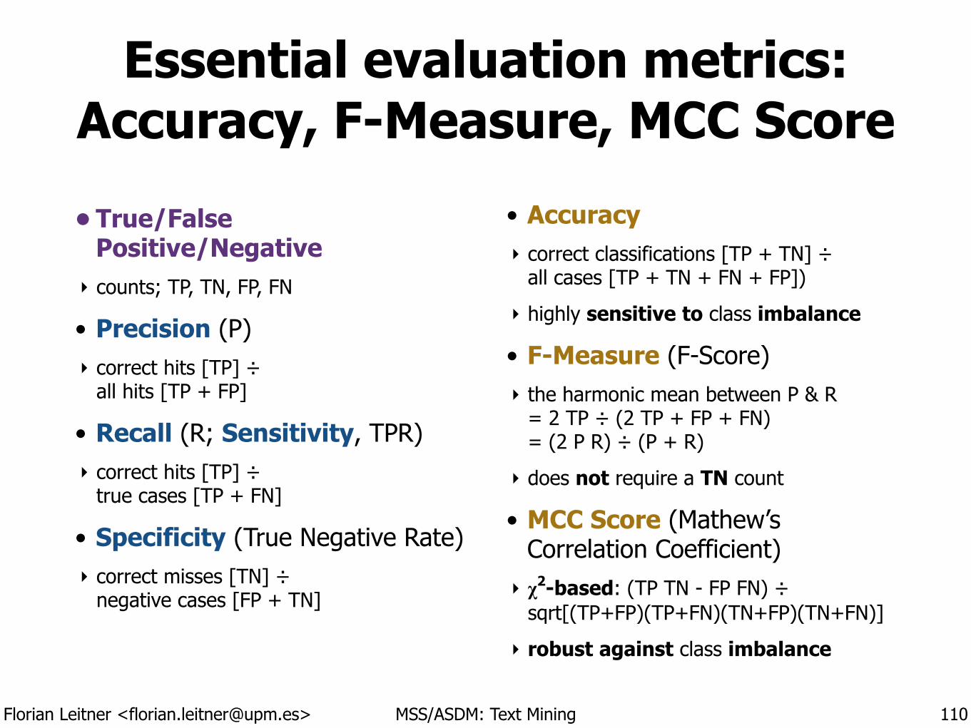
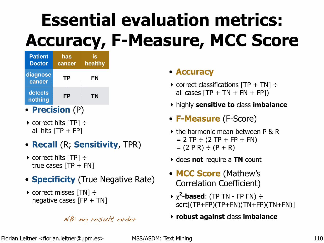
Essential evaluation metrics: Accuracy, F-Measure, MCC Score
• True/False Positive/Negative
‣ counts; TP, TN, FP, FN
• Precision (P) ‣ correct hits [TP] ÷
all hits [TP + FP]
• Recall (R; Sensitivity, TPR) ‣ correct hits [TP] ÷
true cases [TP + FN]
• Specificity (True Negative Rate) ‣ correct misses [TN] ÷
negative cases [FP + TN]
!
• Accuracy ‣ correct classifications [TP + TN] ÷
all cases [TP + TN + FN + FP])
‣ highly sensitive to class imbalance
• F-Measure (F-Score) ‣ the harmonic mean between P & R
= 2 TP ÷ (2 TP + FP + FN)= (2 P R) ÷ (P + R)
‣ does not require a TN count
• MCC Score (Mathew’s Correlation Coefficient)
‣ χ2-based: (TP TN - FP FN) ÷sqrt[(TP+FP)(TP+FN)(TN+FP)(TN+FN)]
‣ robust against class imbalance
110
Florian Leitner <[email protected]> MSS/ASDM: Text Mining
Essential evaluation metrics: Accuracy, F-Measure, MCC Score
• True/False Positive/Negative
‣ counts; TP, TN, FP, FN
• Precision (P) ‣ correct hits [TP] ÷
all hits [TP + FP]
• Recall (R; Sensitivity, TPR) ‣ correct hits [TP] ÷
true cases [TP + FN]
• Specificity (True Negative Rate) ‣ correct misses [TN] ÷
negative cases [FP + TN]
!
• Accuracy ‣ correct classifications [TP + TN] ÷
all cases [TP + TN + FN + FP])
‣ highly sensitive to class imbalance
• F-Measure (F-Score) ‣ the harmonic mean between P & R
= 2 TP ÷ (2 TP + FP + FN)= (2 P R) ÷ (P + R)
‣ does not require a TN count
• MCC Score (Mathew’s Correlation Coefficient)
‣ χ2-based: (TP TN - FP FN) ÷sqrt[(TP+FP)(TP+FN)(TN+FP)(TN+FN)]
‣ robust against class imbalance
110
NB: no result order
Patient!Doctor
has cancer
is healthy
diagnose cancer TP FN
detects nothing FP TN
Florian Leitner <[email protected]> MSS/ASDM: Text Mining
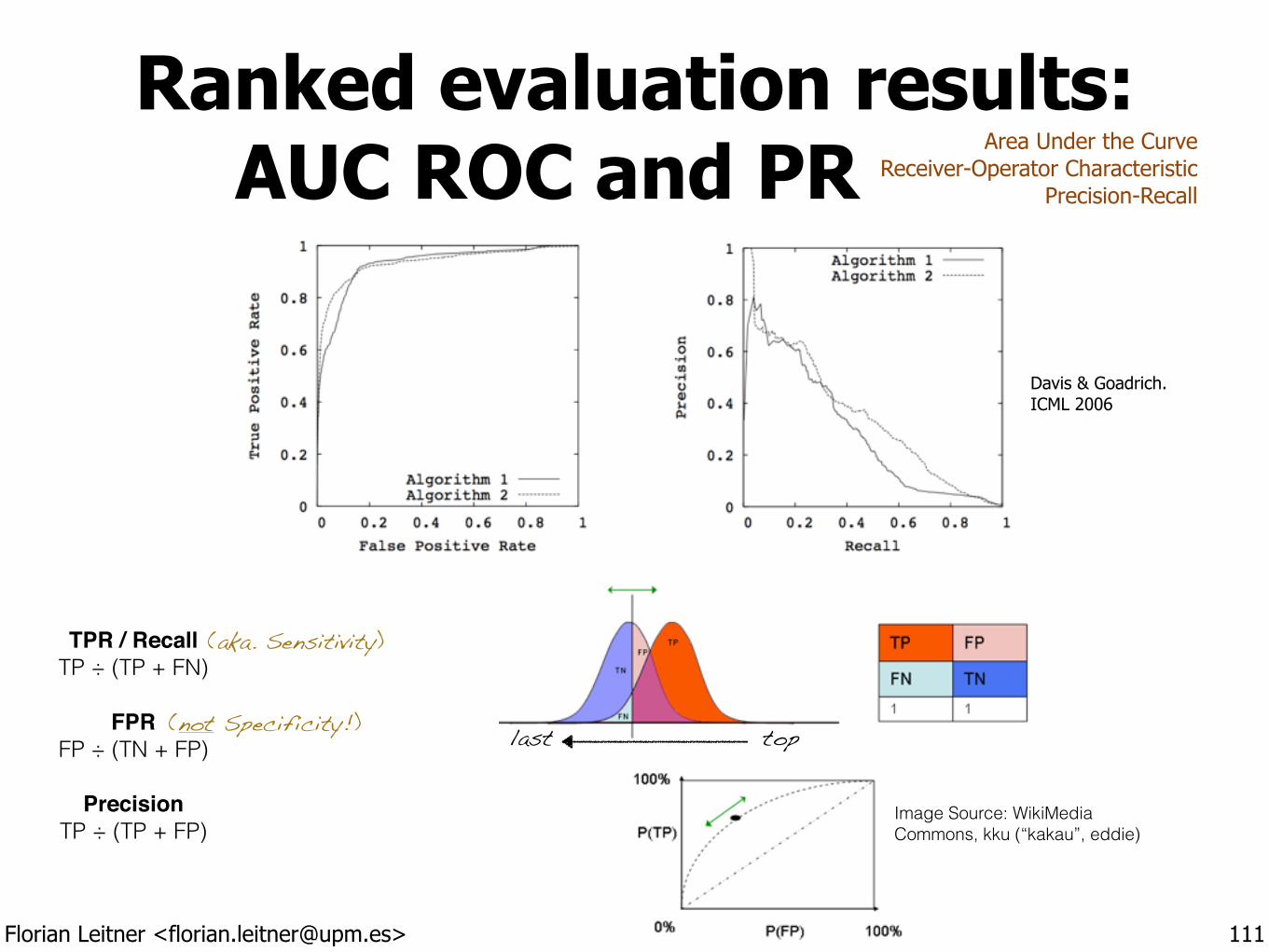
Ranked evaluation results: AUC ROC and PR .
111
Image Source: WikiMedia Commons, kku (“kakau”, eddie)
Area Under the Curve Receiver-Operator Characteristic
Precision-Recall
TPR / Recall!TP ÷ (TP + FN)
!FPR!
FP ÷ (TN + FP) !
Precision!TP ÷ (TP + FP)
(aka. Sensitivity)
(not Specificity!)
Davis & Goadrich.ICML 2006
toplast
Florian Leitner <[email protected]> MSS/ASDM: Text Mining
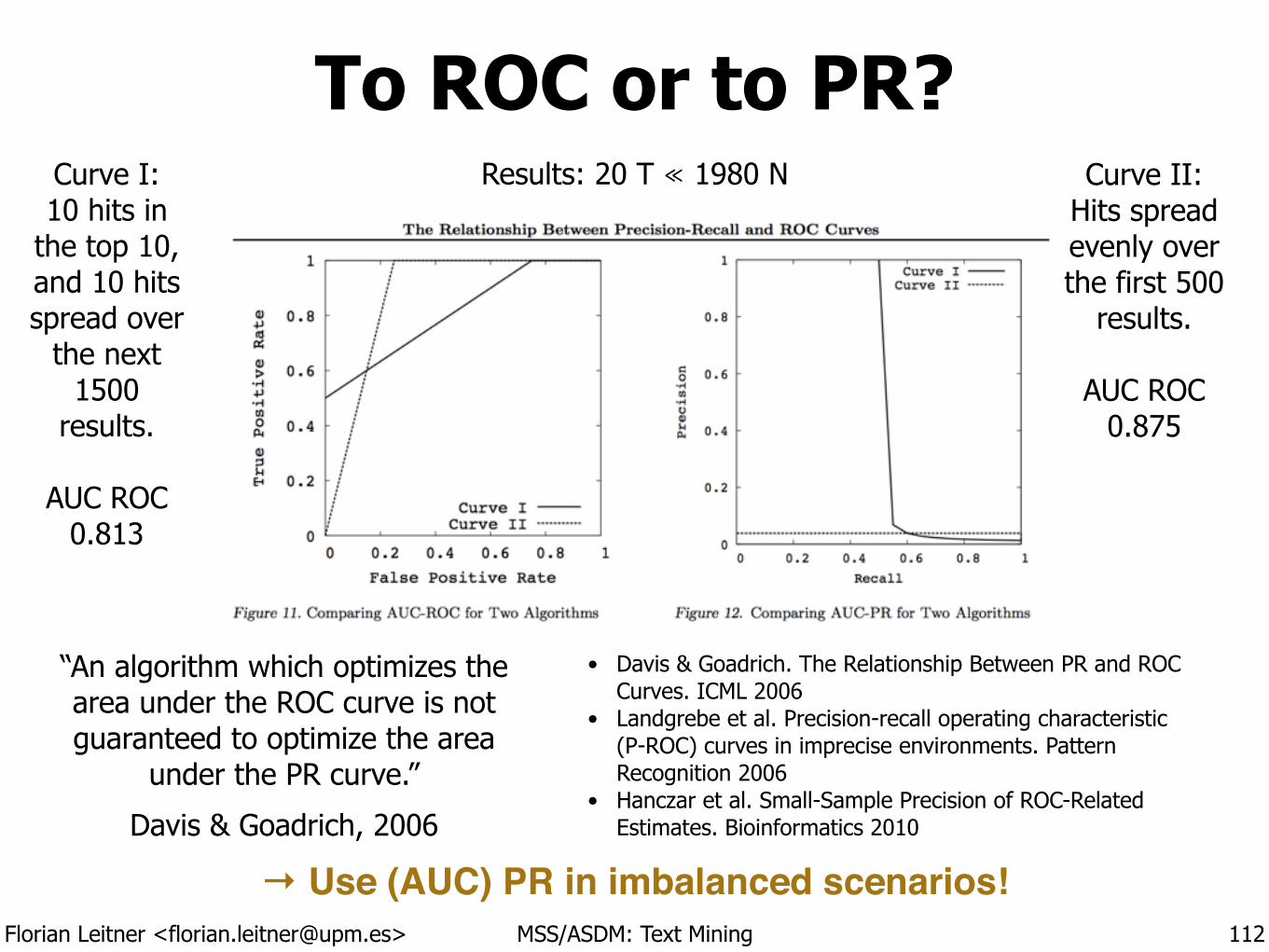
To ROC or to PR?
112
• Davis & Goadrich. The Relationship Between PR and ROC Curves. ICML 2006
• Landgrebe et al. Precision-recall operating characteristic (P-ROC) curves in imprecise environments. Pattern Recognition 2006
• Hanczar et al. Small-Sample Precision of ROC-Related Estimates. Bioinformatics 2010
“An algorithm which optimizes the area under the ROC curve is not guaranteed to optimize the area
under the PR curve.”
Davis & Goadrich, 2006
Curve I: 10 hits in
the top 10, and 10 hits spread over
the next 1500
results. !
AUC ROC 0.813
Curve II: Hits spread evenly over the first 500
results. !
AUC ROC 0.875
Results: 20 T ≪ 1980 N
→ Use (AUC) PR in imbalanced scenarios!
Florian Leitner <[email protected]> MSS/ASDM: Text Mining
Sentiment Analysis
as an example domain for text classification
(only if there is time left after the exercises)
!
113
Cristopher Potts. Sentiment Symposium Tutorial. 2011 http://sentiment.christopherpotts.net/index.html
Florian Leitner <[email protected]> MSS/ASDM: Text Mining
Opinion/Sentiment Analysis
• Harder than “regular” document classification ‣ irony, neutral (“non-polar”) sentiment, negations (“not good”),
syntax is used to express emotions (“!”), context dependent
• Confounding polarities from individual aspects (phrases) ‣ e.g., a car company’s “customer service” vs. the “safety” of their cars
• Strong commercial interest in this topic ‣ “Social” (commercial?) networking sites (FB, G+, …; advertisement)
‣ Reviews (Amazon, Google Maps), blogs, fora, online comments, …
‣ Brand reputation and political opinion analysis
114
Florian Leitner <[email protected]> MSS/ASDM: Text Mining
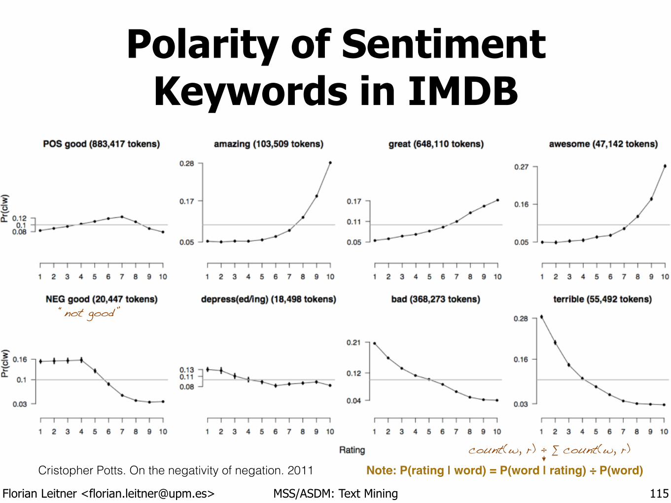
Polarity of Sentiment Keywords in IMDB
115
Cristopher Potts. On the negativity of negation. 2011 Note: P(rating | word) = P(word | rating) ÷ P(word)count(w, r) ÷ ∑ count(w, r)
“not good”
Florian Leitner <[email protected]> MSS/ASDM: Text Mining
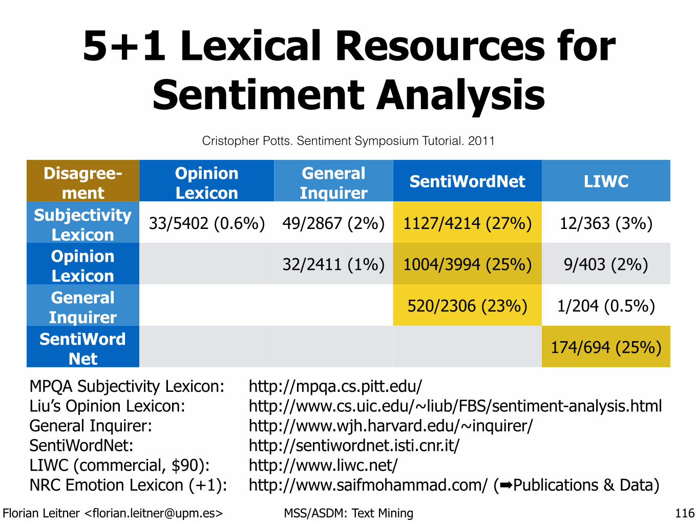
5+1 Lexical Resources for Sentiment Analysis
116
Disagree-ment
Opinion Lexicon
General Inquirer
SentiWordNet LIWC
Subjectivity Lexicon
33/5402 (0.6%) 49/2867 (2%) 1127/4214 (27%) 12/363 (3%)
Opinion Lexicon
32/2411 (1%) 1004/3994 (25%) 9/403 (2%)
General Inquirer
520/2306 (23%) 1/204 (0.5%)
SentiWord Net
174/694 (25%)
MPQA Subjectivity Lexicon: http://mpqa.cs.pitt.edu/ Liu’s Opinion Lexicon: http://www.cs.uic.edu/~liub/FBS/sentiment-analysis.html General Inquirer: http://www.wjh.harvard.edu/~inquirer/ SentiWordNet: http://sentiwordnet.isti.cnr.it/ LIWC (commercial, $90): http://www.liwc.net/ NRC Emotion Lexicon (+1): http://www.saifmohammad.com/ (➡Publications & Data)
Cristopher Potts. Sentiment Symposium Tutorial. 2011
Florian Leitner <[email protected]> MSS/ASDM: Text Mining
Detecting the Sentiment of Individual Aspects
• Goal: Determine the sentiment for a particular aspect or establish their polarity.
‣ An “aspect” here is a phrase or concept, like “customer service”.
‣ “They have a great+ customer service team, but the delivery took ages-.”
• Solution: Measure the co-occurrence of the aspect with words of distinct sentiment or relative co-occurrence with words of the same polarity.
‣ The “sentiment” keywords are taken from some lexical resource.
117
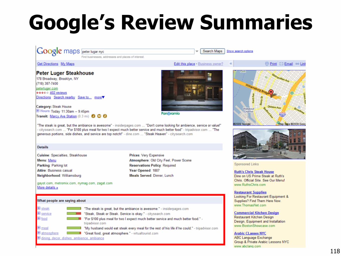
Google’s Review Summaries
118
Florian Leitner <[email protected]> MSS/ASDM: Text Mining
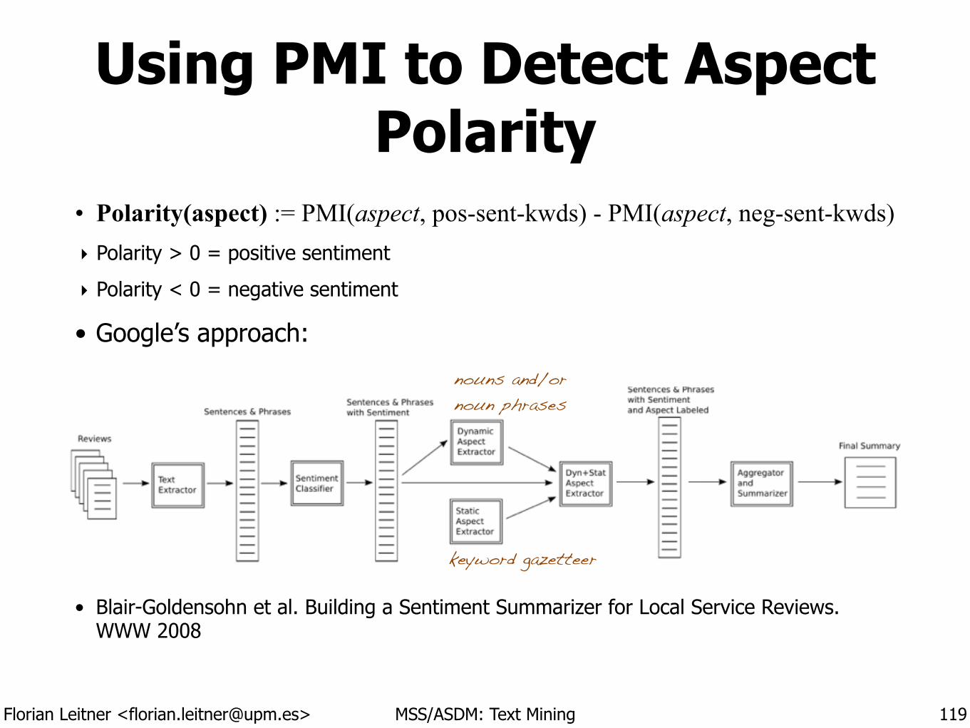
Using PMI to Detect Aspect Polarity
• Polarity(aspect) := PMI(aspect, pos-sent-kwds) - PMI(aspect, neg-sent-kwds) ‣ Polarity > 0 = positive sentiment
‣ Polarity < 0 = negative sentiment
• Google’s approach:
!
!
!
!
!• Blair-Goldensohn et al. Building a Sentiment Summarizer for Local Service Reviews.
WWW 2008
119
nouns and/or noun phrases
keyword gazetteer
Text Mining 5 Information Extraction
!Madrid Summer School on
Advanced Statistics and Data Mining !
Florian Leitner [email protected]
License:
Florian Leitner <[email protected]> MSS/ASDM: Text Mining
Retrospective
We have seen how to…
• Design generative models of natural language.
• Segment, tokenize, and compare text and/or sentences.
• [Multi-] labeling whole documents or chunks of text.
!
Some open questions…
• How to assign labels to individual tokens in a stream?
‣ without using a dictionary/gazetteer: sequence taggers
• How to detect semantic relationships between tokens?
‣ dependency parsers
121
Florian Leitner <[email protected]> MSS/ASDM: Text Mining
Incentive and applications
➡ Statistical analyses of [token] sequences
!
• Part-of-Speech (PoS) tagging & chunking ‣ noun, verb, adjective, … & noun/verb/preposition/… phrases
• Named Entity Recognition (NER) ‣ organizations, persons, places, genes, chemicals, …
• Information extraction ‣ locations/times, phys. constants & chem. formulas, entity linking, event
extraction, entity-relationship extraction, …
122
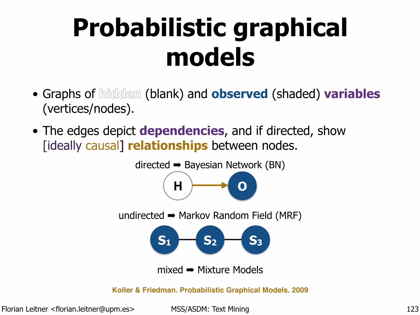
Florian Leitner <[email protected]> MSS/ASDM: Text Mining
Probabilistic graphical models
• Graphs of hidden (blank) and observed (shaded) variables (vertices/nodes).
• The edges depict dependencies, and if directed, show [ideally causal] relationships between nodes.
123
H O
S3S2S1
directed ➡ Bayesian Network (BN)
undirected ➡ Markov Random Field (MRF)
mixed ➡ Mixture Models
Koller & Friedman. Probabilistic Graphical Models. 2009
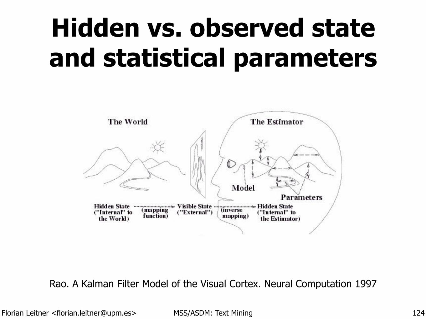
Florian Leitner <[email protected]> MSS/ASDM: Text Mining
Hidden vs. observed state and statistical parameters
Rao. A Kalman Filter Model of the Visual Cortex. Neural Computation 1997
124
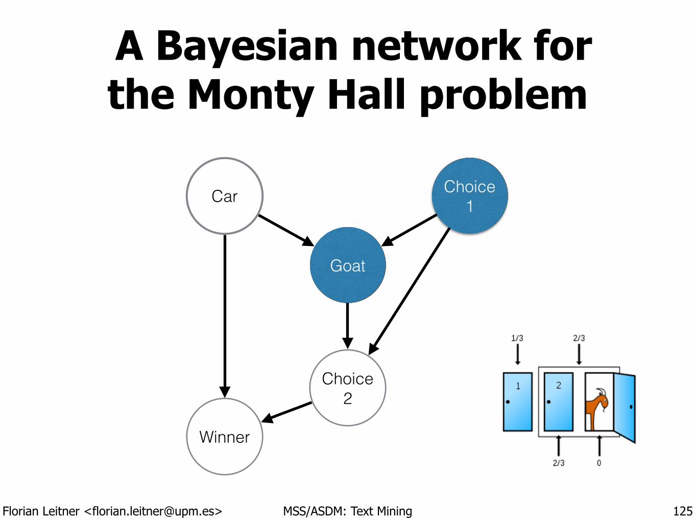
Florian Leitner <[email protected]> MSS/ASDM: Text Mining
A Bayesian network for the Monty Hall problem
125
Choice 1
Choice 2
Goat
Winner
Car
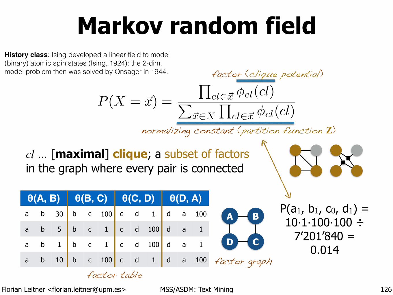
Florian Leitner <[email protected]> MSS/ASDM: Text Mining
Markov random field
126
normalizing constant (partition function Z)
factor (clique potential)
A
D
B
C
θ(A, B) θ(B, C) θ(C, D) θ(D, A)a b 30 b c 100 c d 1 d a 100
a b 5 b c 1 c d 100 d a 1
a b 1 b c 1 c d 100 d a 1
a b 10 b c 100 c d 1 d a 100
P(a1, b1, c0, d1) = 10·1·100·100 ÷
7’201’840 = 0.014
factor tablefactor graph
P (X = ~x) =
Qcl2~x
�
cl
(cl)P~x2X
Qcl2~x
�
cl
(cl)
cl … [maximal] clique; a subset of factors in the graph where every pair is connected
History class: Ising developed a linear field to model (binary) atomic spin states (Ising, 1924); the 2-dim. model problem then was solved by Onsager in 1944.
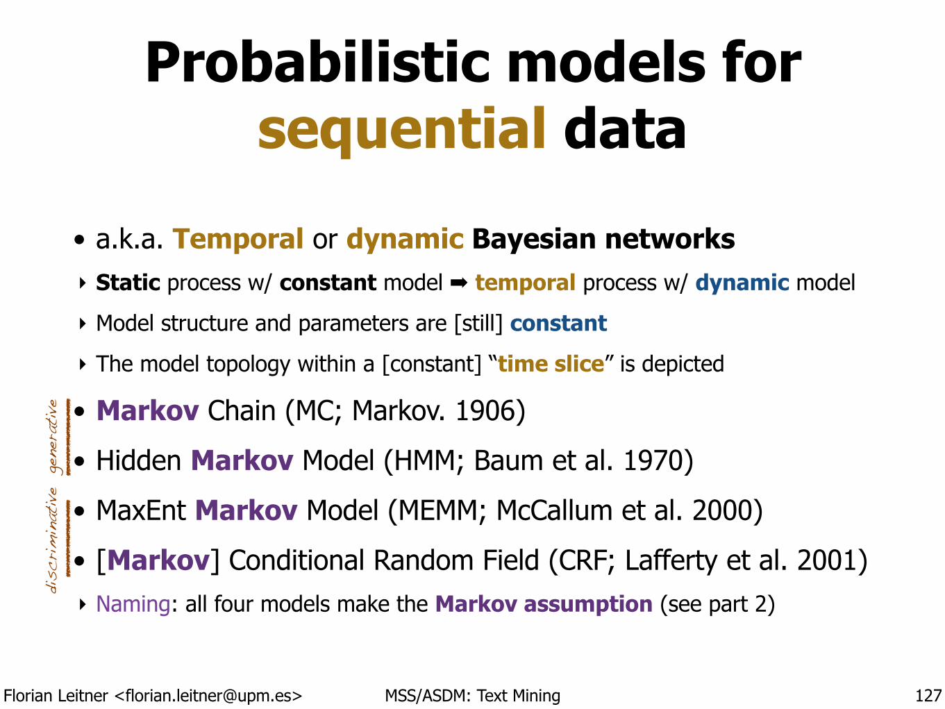
Florian Leitner <[email protected]> MSS/ASDM: Text Mining
Probabilistic models for sequential data
• a.k.a. Temporal or dynamic Bayesian networks ‣ Static process w/ constant model ➡ temporal process w/ dynamic model
‣ Model structure and parameters are [still] constant
‣ The model topology within a [constant] “time slice” is depicted
• Markov Chain (MC; Markov. 1906)
• Hidden Markov Model (HMM; Baum et al. 1970)
• MaxEnt Markov Model (MEMM; McCallum et al. 2000)
• [Markov] Conditional Random Field (CRF; Lafferty et al. 2001) ‣ Naming: all four models make the Markov assumption (see part 2)
127
gene
rativ
edis
crim
inativ
e
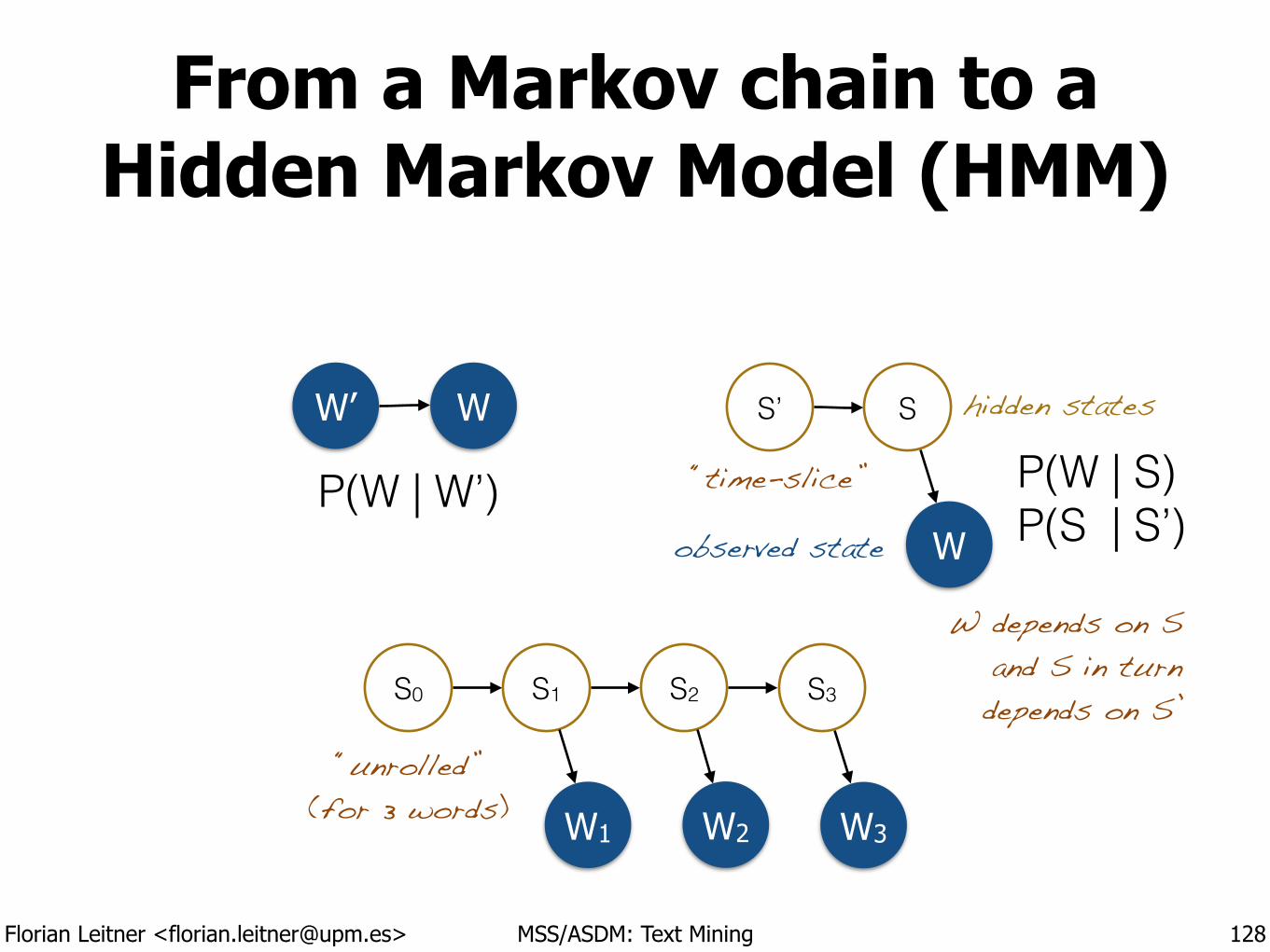
Florian Leitner <[email protected]> MSS/ASDM: Text Mining
From a Markov chain to a Hidden Markov Model (HMM)
128
WW’ SS’
W
hidden states
observed state
S1S0
W1
S2
W2
S3
W3
“unrolled” (for 3 words)
“time-slice”
W depends on S and S in turn depends on S’
P(W | W’) P(W | S) P(S | S’)
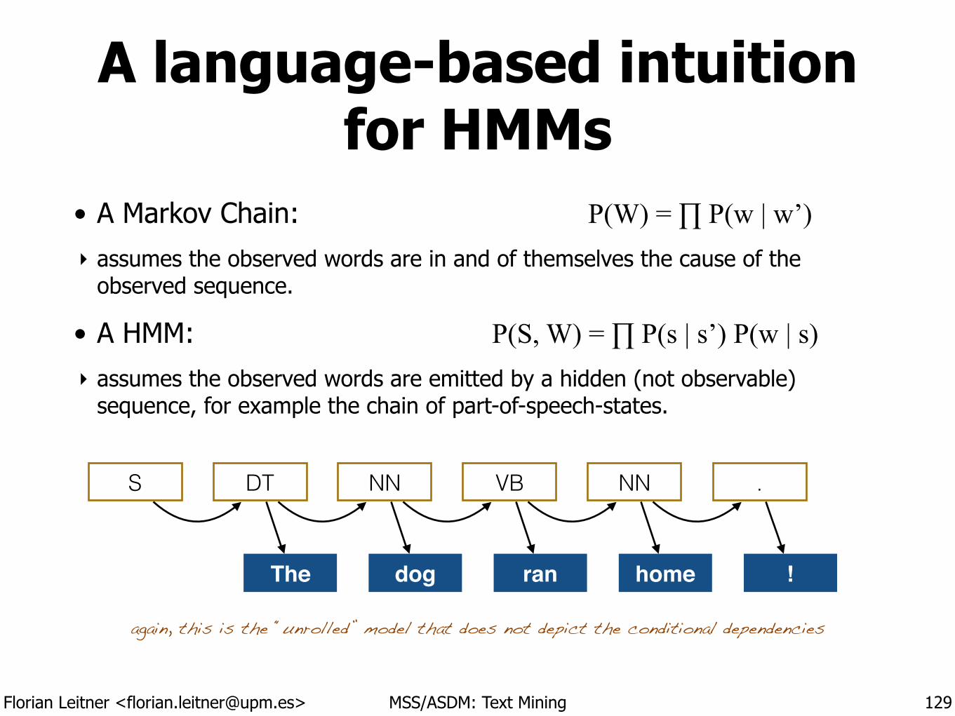
Florian Leitner <[email protected]> MSS/ASDM: Text Mining
A language-based intuition for HMMs
• A Markov Chain: P(W) = ∏ P(w | w’) ‣ assumes the observed words are in and of themselves the cause of the
observed sequence.
• A HMM: P(S, W) = ∏ P(s | s’) P(w | s) ‣ assumes the observed words are emitted by a hidden (not observable)
sequence, for example the chain of part-of-speech-states.
129
S DT NN VB NN .
The dog ran home !
again, this is the “unrolled” model that does not depict the conditional dependencies
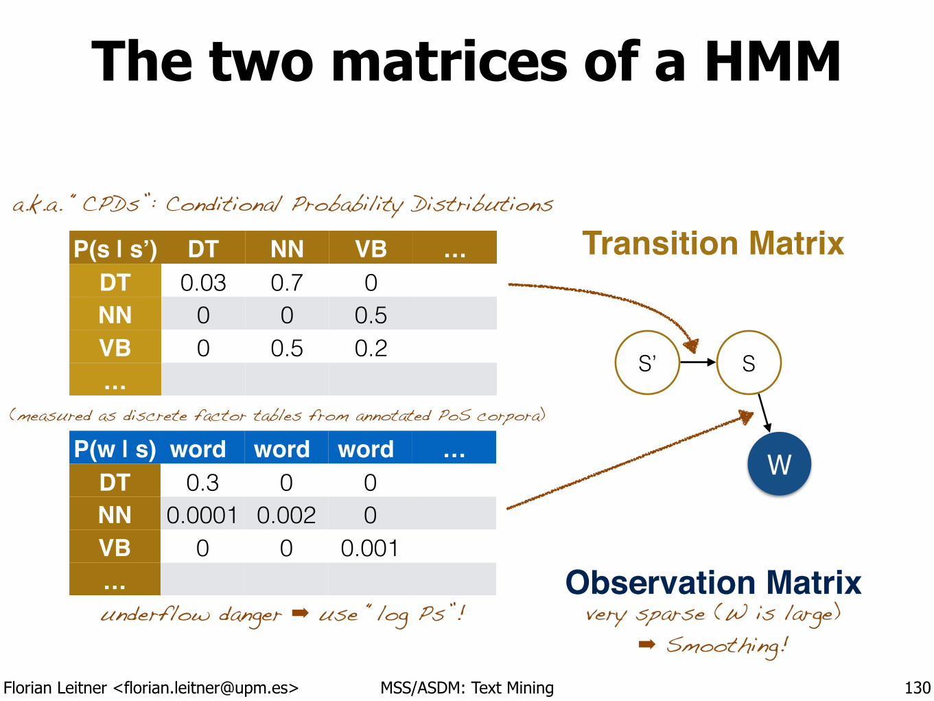
Florian Leitner <[email protected]> MSS/ASDM: Text Mining
The two matrices of a HMM
130
P(s | s’) DT NN VB …DT 0.03 0.7 0NN 0 0 0.5VB 0 0.5 0.2…
P(w | s) word word word …DT 0.3 0 0NN 0.0001 0.002 0VB 0 0 0.001…
SS’
W
very sparse (W is large) ➡ Smoothing!
Transition Matrix
Observation Matrixunderflow danger ➡ use “log Ps”!
a.k.a. “CPDs”: Conditional Probability Distributions
(measured as discrete factor tables from annotated PoS corpora)
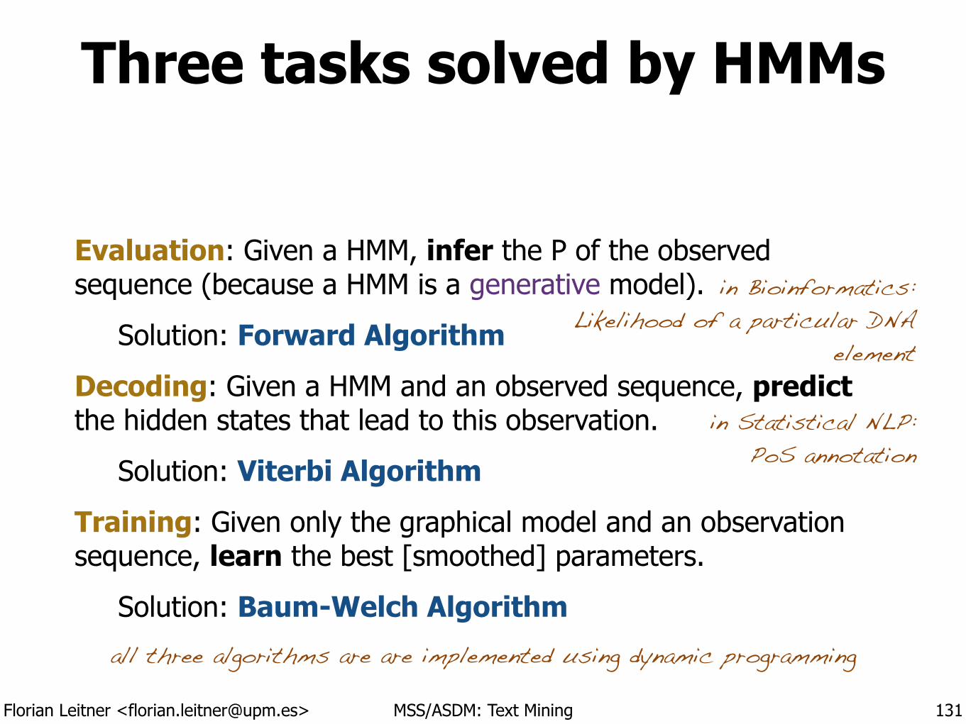
Florian Leitner <[email protected]> MSS/ASDM: Text Mining
Three tasks solved by HMMs
Evaluation: Given a HMM, infer the P of the observed sequence (because a HMM is a generative model).
Solution: Forward Algorithm
Decoding: Given a HMM and an observed sequence, predict the hidden states that lead to this observation.
Solution: Viterbi Algorithm
Training: Given only the graphical model and an observation sequence, learn the best [smoothed] parameters.
Solution: Baum-Welch Algorithm
131
all three algorithms are are implemented using dynamic programming
in Bioinformatics: Likelihood of a particular DNA
element
in Statistical NLP: PoS annotation
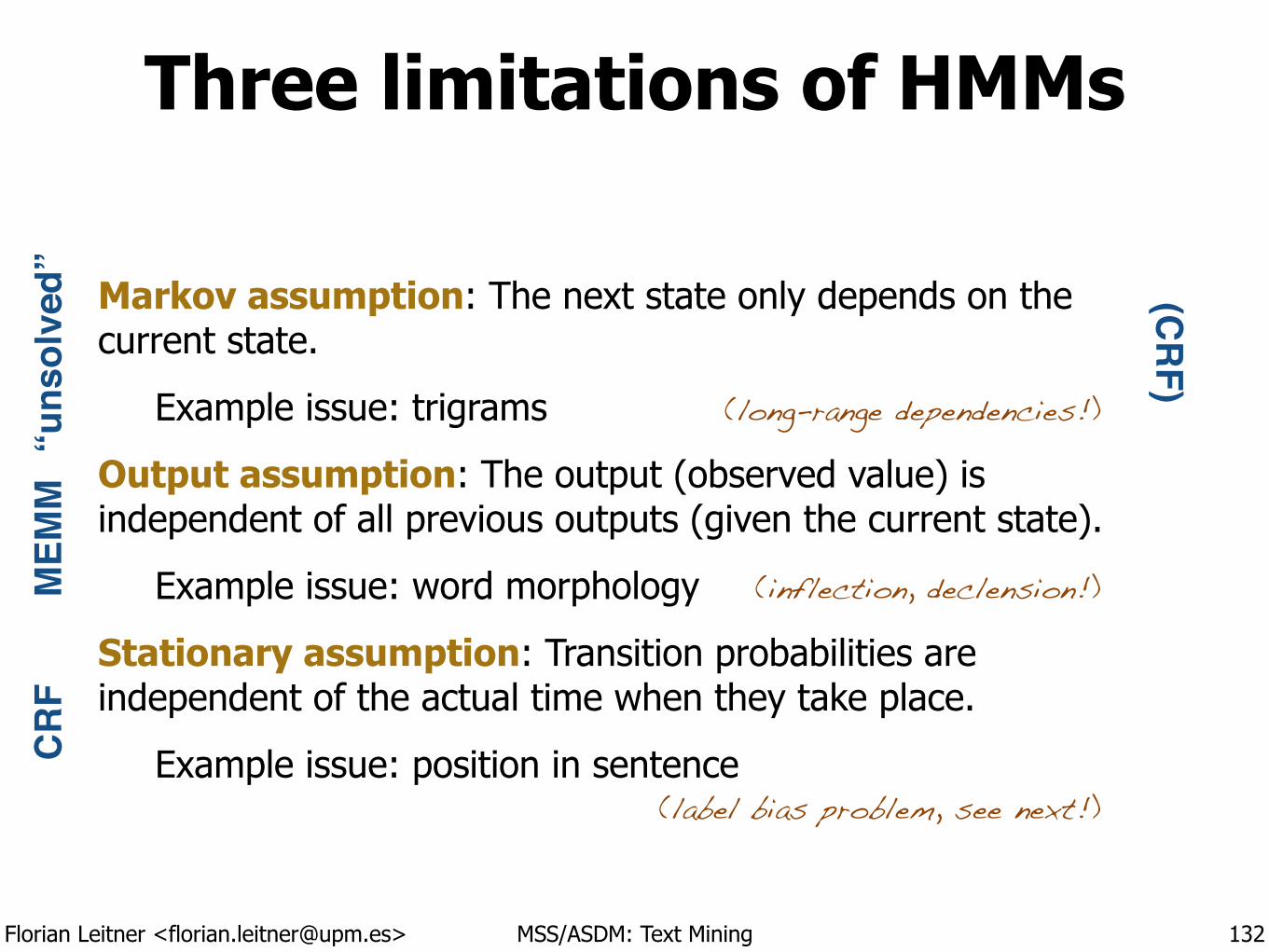
Florian Leitner <[email protected]> MSS/ASDM: Text Mining
Three limitations of HMMs
Markov assumption: The next state only depends on the current state.
Example issue: trigrams
Output assumption: The output (observed value) is independent of all previous outputs (given the current state).
Example issue: word morphology
Stationary assumption: Transition probabilities are independent of the actual time when they take place.
Example issue: position in sentence
132
(label bias problem, see next!)
(long-range dependencies!)
(inflection, declension!)MEM
MCR
F“u
nsol
ved” (CRF)
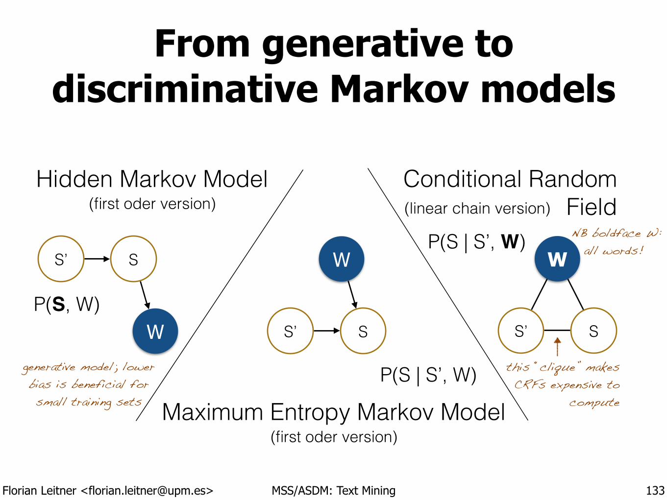
Florian Leitner <[email protected]> MSS/ASDM: Text Mining
From generative to discriminative Markov models
133
SS’
W S’ S
W
S’ S
W
Hidden Markov Model
Maximum Entropy Markov Model
Conditional RandomField
this “clique” makes CRFs expensive to
compute
generative model; lower bias is beneficial for small training sets
(linear chain version)(first oder version)
P(S, W)
P(S | S’, W)
NB boldface W: all words!
(first oder version)
P(S | S’, W)
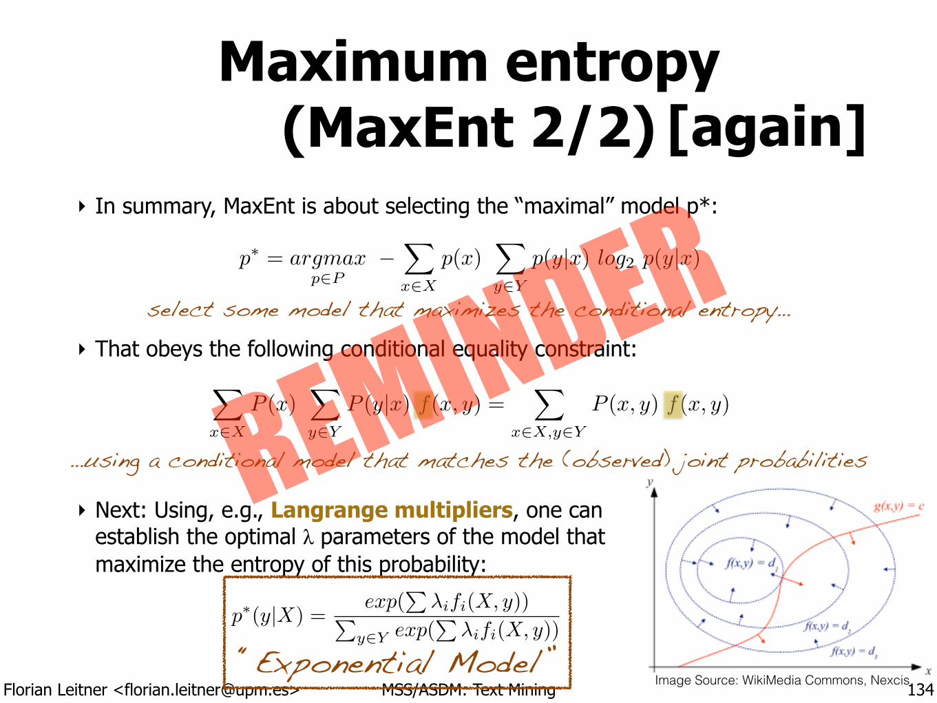
Florian Leitner <[email protected]> MSS/ASDM: Text Mining
Maximum entropy (MaxEnt 2/2)
‣ In summary, MaxEnt is about selecting the “maximal” model p*: !!!
‣ That obeys the following conditional equality constraint:
!
!
!
‣ Next: Using, e.g., Langrange multipliers, one canestablish the optimal λ parameters of the model that maximize the entropy of this probability:
134
X
x2X
P (x)X
y2Y
P (y|x) f(x, y) =X
x2X,y2Y
P (x, y) f(x, y)
p
⇤ = argmax
p2P
�X
x2X
p(x)X
y2Y
p(y|x) log2 p(y|x)
…using a conditional model that matches the (observed) joint probabilities
select some model that maximizes the conditional entropy…
[again]
Image Source: WikiMedia Commons, Nexcis
p
⇤(y|X) =exp(
P�ifi(X, y))P
y2Y exp(P
�ifi(X, y))
REMINDER
“Exponential Model”
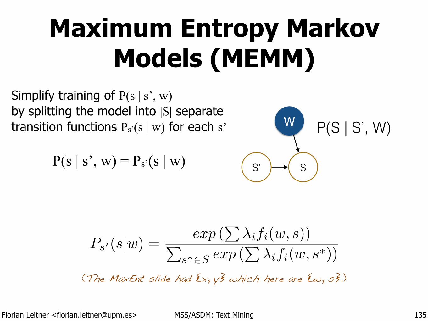
Florian Leitner <[email protected]> MSS/ASDM: Text Mining
Maximum Entropy Markov Models (MEMM)
Simplify training of P(s | s’, w)by splitting the model into |S| separate transition functions Ps’(s | w) for each s’
135
P(S | S’, W)
S’ S
W
Ps0(s|w) =exp (
P�ifi(w, s))P
s⇤2S exp (P
�ifi(w, s⇤))
P(s | s’, w) = Ps’(s | w)
(The MaxEnt slide had {x, y} which here are {w, s}.)
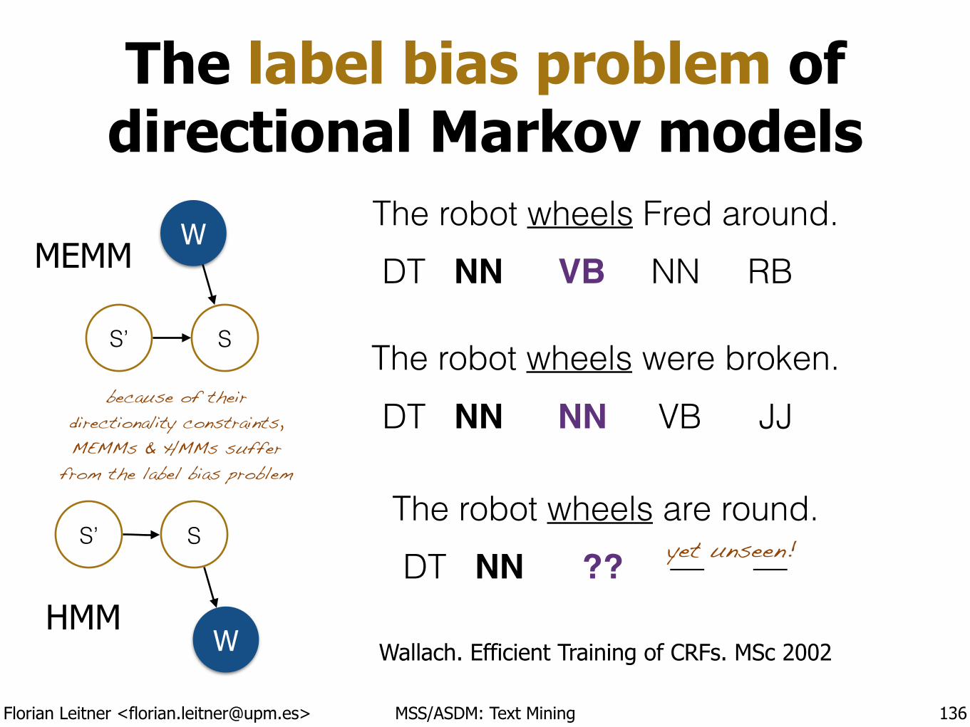
Florian Leitner <[email protected]> MSS/ASDM: Text Mining
The label bias problem of directional Markov models
136
The robot wheels are round.
The robot wheels Fred around.
The robot wheels were broken.
DT NN VB NN RB
DT NN NN VB JJ
DT NN ?? — —yet unseen!
Wallach. Efficient Training of CRFs. MSc 2002
because of their directionality constraints, MEMMs & HMMs suffer
from the label bias problem
S’ S
WMEMM
HMM
SS’
W
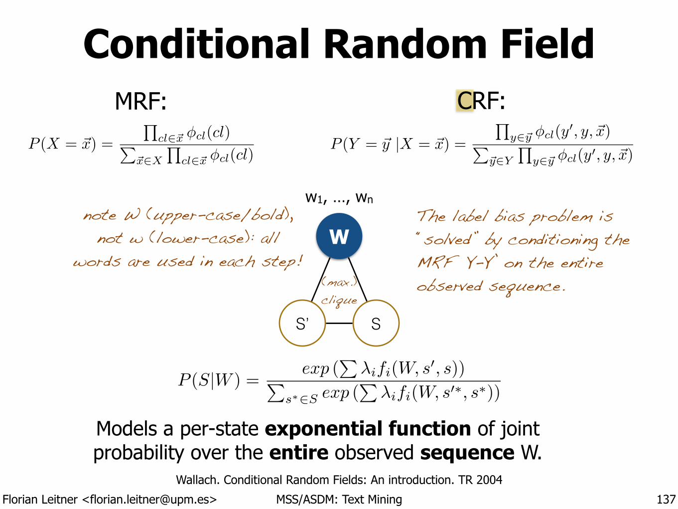
Florian Leitner <[email protected]> MSS/ASDM: Text Mining
Conditional Random Field
137
SS’
W
w1, …, wn
Models a per-state exponential function of joint probability over the entire observed sequence W.
(max.) clique
MRF:
The label bias problem is “solved” by conditioning the MRF Y-Y’ on the entire observed sequence.
CRF:
note W (upper-case/bold), not w (lower-case): all
words are used in each step!
P (X = ~x) =
Qcl2~x
�
cl
(cl)P~x2X
Qcl2~x
�
cl
(cl)P (Y = ~y |X = ~x) =
Qy2~y �cl(y0, y, ~x)P
~y2Y
Qy2~y �cl(y0, y, ~x)
P (S|W ) =exp (
P�ifi(W, s
0, s))P
s⇤2S exp (P
�ifi(W, s
0⇤, s
⇤))
Wallach. Conditional Random Fields: An introduction. TR 2004
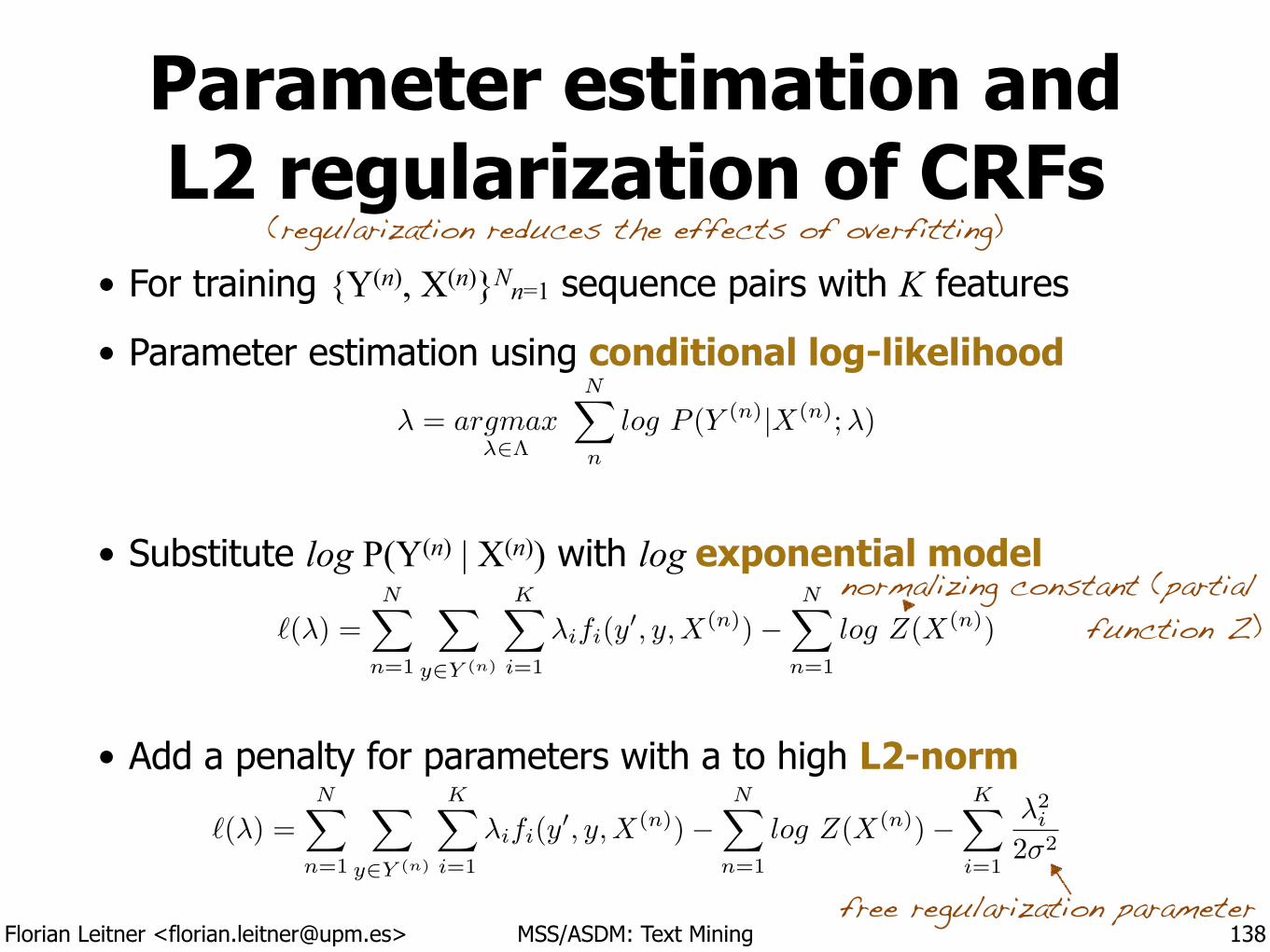
Florian Leitner <[email protected]> MSS/ASDM: Text Mining
Parameter estimation and L2 regularization of CRFs
• For training {Y(n), X(n)}Nn=1 sequence pairs with K features
• Parameter estimation using conditional log-likelihood
!
!
• Substitute log P(Y(n) | X(n)) with log exponential model
!
!
• Add a penalty for parameters with a to high L2-norm
138free regularization parameter
`(�) =NX
n=1
X
y2Y (n)
KX
i=1
�ifi(y0, y,X
(n))�NX
n=1
log Z(X(n))
`(�) =NX
n=1
X
y2Y (n)
KX
i=1
�ifi(y0, y,X
(n))�NX
n=1
log Z(X(n))�KX
i=1
�
2i
2�2
(regularization reduces the effects of overfitting)
normalizing constant (partial function Z)
� = argmax
�2⇤
NX
n
log P (Y (n)|X(n);�)
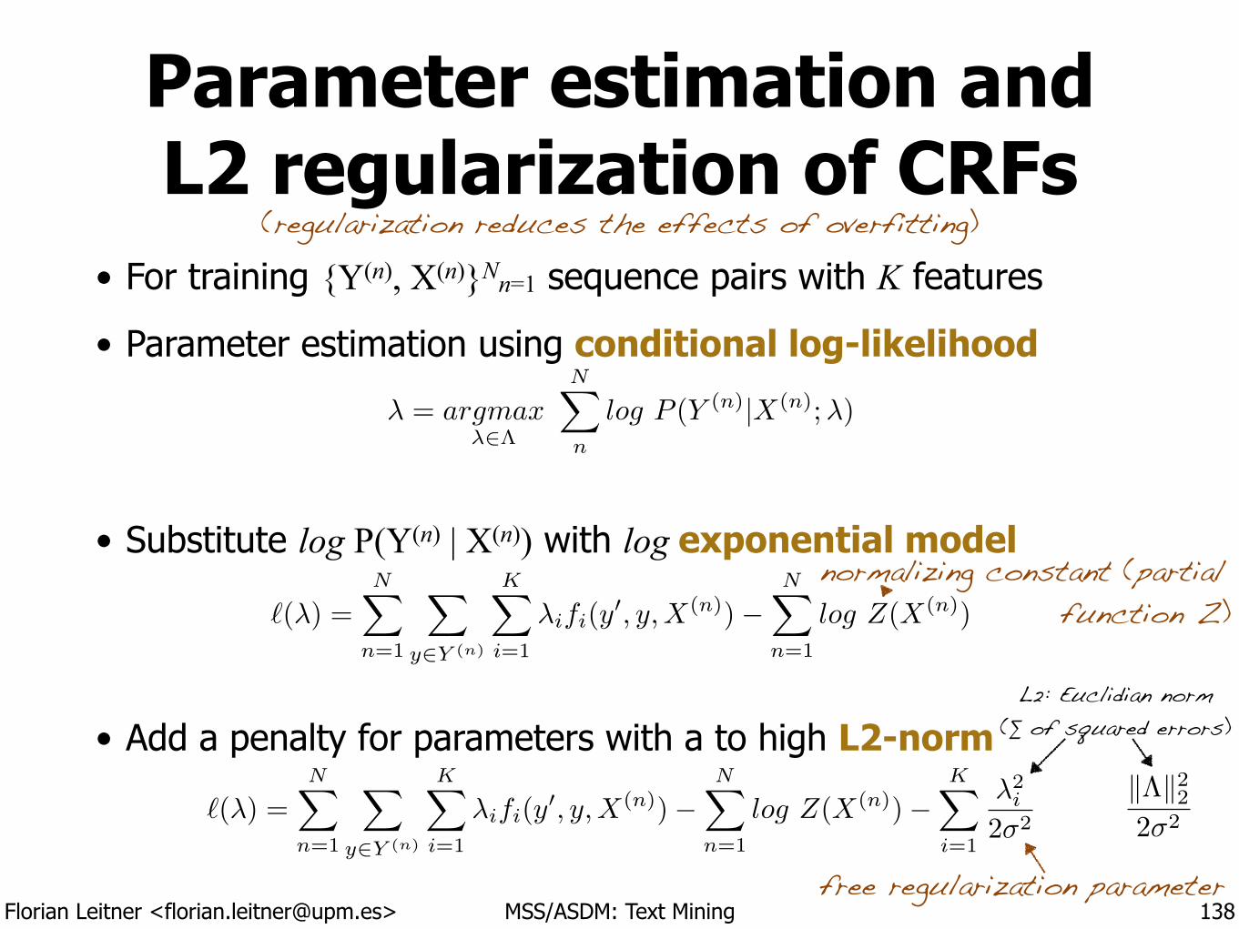
L2: Euclidian norm (∑ of squared errors)
k⇤k222�2
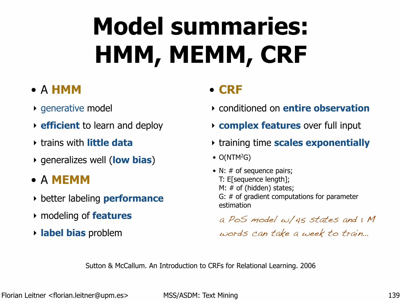
Florian Leitner <[email protected]> MSS/ASDM: Text Mining
Model summaries: HMM, MEMM, CRF
• A HMM ‣ generative model
‣ efficient to learn and deploy
‣ trains with little data
‣ generalizes well (low bias)
• A MEMM ‣ better labeling performance
‣ modeling of features
‣ label bias problem
!
• CRF ‣ conditioned on entire observation
‣ complex features over full input
‣ training time scales exponentially • O(NTM2G)
• N: # of sequence pairs;T: E[sequence length];M: # of (hidden) states;G: # of gradient computations for parameter estimation
139
a PoS model w/45 states and 1 M words can take a week to train…
Sutton & McCallum. An Introduction to CRFs for Relational Learning. 2006
Florian Leitner <[email protected]> MSS/ASDM: Text Mining
Information extraction: Application of dynamic
graphical models
140
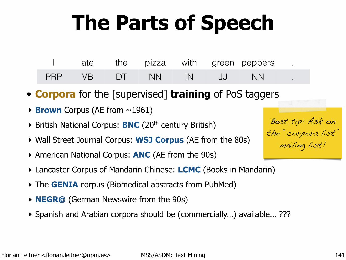
Florian Leitner <[email protected]> MSS/ASDM: Text Mining
The Parts of Speech
• Corpora for the [supervised] training of PoS taggers ‣ Brown Corpus (AE from ~1961)
‣ British National Corpus: BNC (20th century British)
‣ Wall Street Journal Corpus: WSJ Corpus (AE from the 80s)
‣ American National Corpus: ANC (AE from the 90s)
‣ Lancaster Corpus of Mandarin Chinese: LCMC (Books in Mandarin)
‣ The GENIA corpus (Biomedical abstracts from PubMed)
‣ NEGR@ (German Newswire from the 90s)
‣ Spanish and Arabian corpora should be (commercially…) available… ???
141
I ate the pizza with green peppers .PRP VB DT NN IN JJ NN .
!Best tip: Ask on the “corpora list”
mailing list!
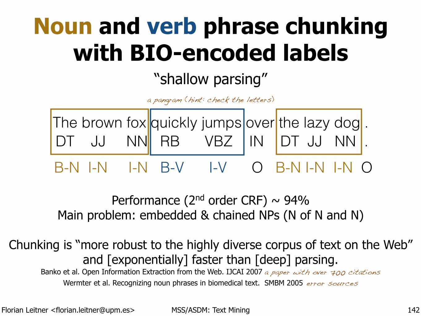
Florian Leitner <[email protected]> MSS/ASDM: Text Mining
Noun and verb phrase chunking with BIO-encoded labels
142
The brown fox quickly jumps over the lazy dog .a pangram (hint: check the letters)
DT JJ NN RB VBZ IN DT JJ NN .B-N I-N I-N B-V I-V O B-N I-N I-N O
Performance (2nd order CRF) ~ 94% Main problem: embedded & chained NPs (N of N and N)
!Chunking is “more robust to the highly diverse corpus of text on the Web”
and [exponentially] faster than [deep] parsing. Banko et al. Open Information Extraction from the Web. IJCAI 2007 a paper with over 700 citations
Wermter et al. Recognizing noun phrases in biomedical text. SMBM 2005 error sources
“shallow parsing”
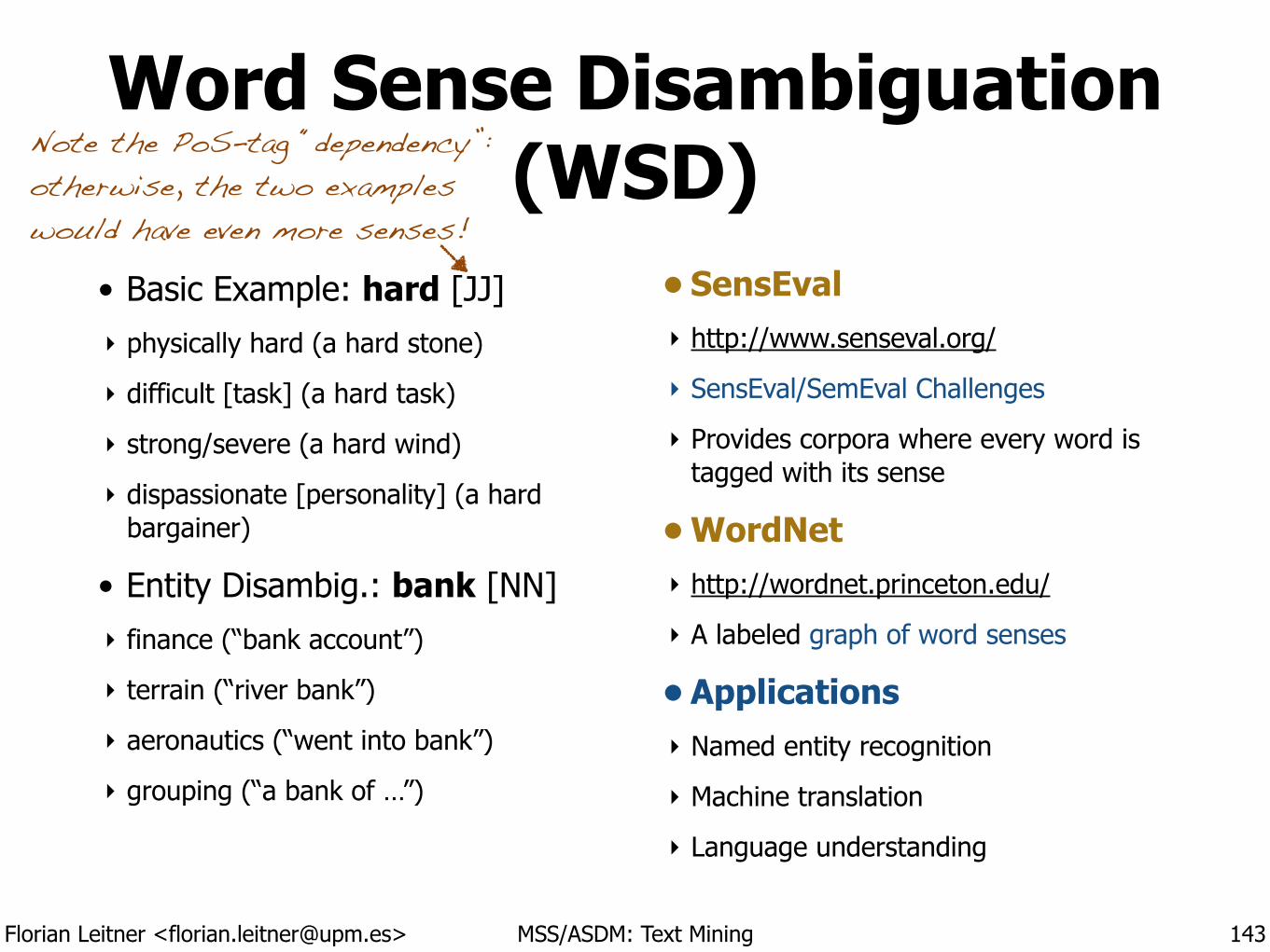
Florian Leitner <[email protected]> MSS/ASDM: Text Mining
Word Sense Disambiguation (WSD)
• Basic Example: hard [JJ] ‣ physically hard (a hard stone)
‣ difficult [task] (a hard task)
‣ strong/severe (a hard wind)
‣ dispassionate [personality] (a hard bargainer)
• Entity Disambig.: bank [NN] ‣ finance (“bank account”)
‣ terrain (“river bank”)
‣ aeronautics (“went into bank”)
‣ grouping (“a bank of …”)
!
• SensEval ‣ http://www.senseval.org/
‣ SensEval/SemEval Challenges
‣ Provides corpora where every word is tagged with its sense
• WordNet ‣ http://wordnet.princeton.edu/
‣ A labeled graph of word senses
• Applications ‣ Named entity recognition
‣ Machine translation
‣ Language understanding
143
Note the PoS-tag “dependency”: otherwise, the two examples would have even more senses!
Florian Leitner <[email protected]> MSS/ASDM: Text Mining
Word vector representations: Unsupervised WSD
• Idea 1: Words with similar meaning have similar environments.
• Use a word vector to count a word’s surrounding words.
• Similar words now will have similar word vectors. ‣ See lecture 2, neural network models of language and lecture 4, cosine similarity
‣ Visualization: Principal Component Analysis
!
• Idea 2: Words with similar meaning have similar environments.
• Use the surrounding of unseen words to “smoothen” language models (i.e., the correlation between word wi and its context cj).
‣ see Text Mining 4: TF-IDF weighting, Cosine similarity and point-wise MI
‣ Levy & Goldberg. Linguistic Regularities in Sparse and Explicit Word Representations. CoNLL 2014
144
Levy & Goldberg took two words on each side to “beat” a neural
network model with a four word window!
Turian et al. Word representations. ACL 2010
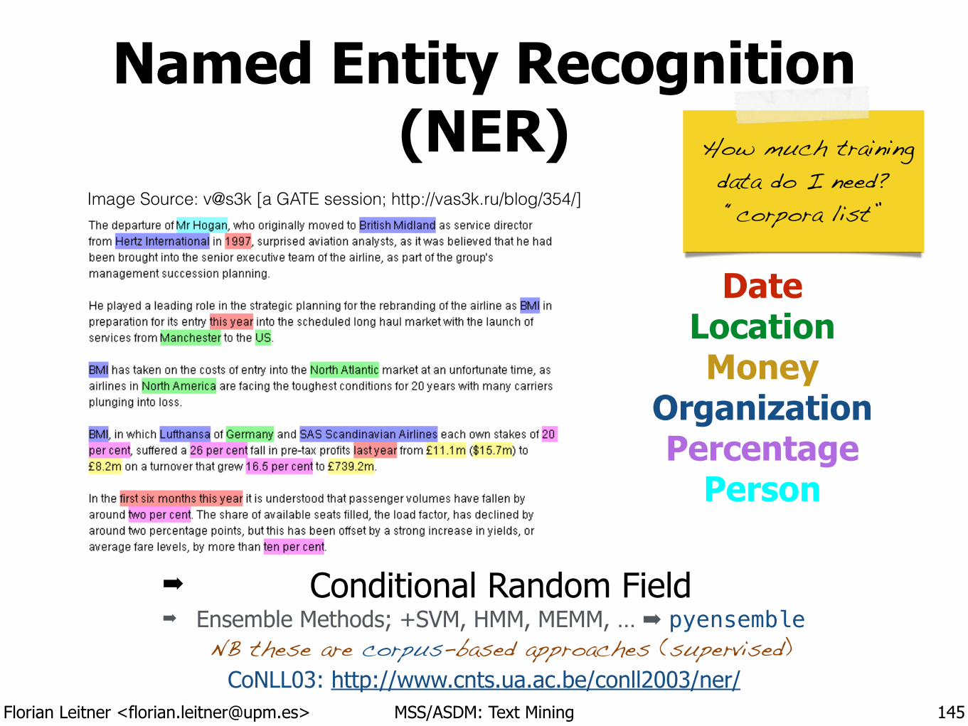
Florian Leitner <[email protected]> MSS/ASDM: Text Mining
Named Entity Recognition (NER)
145
Date Location Money
Organization Percentage
Person
➡ Conditional Random Field ➡ Ensemble Methods; +SVM, HMM, MEMM, … ➡ pyensemble
NB these are corpus-based approaches (supervised)CoNLL03: http://www.cnts.ua.ac.be/conll2003/ner/
! How much training
data do I need? “corpora list” Image Source: v@s3k [a GATE session; http://vas3k.ru/blog/354/]
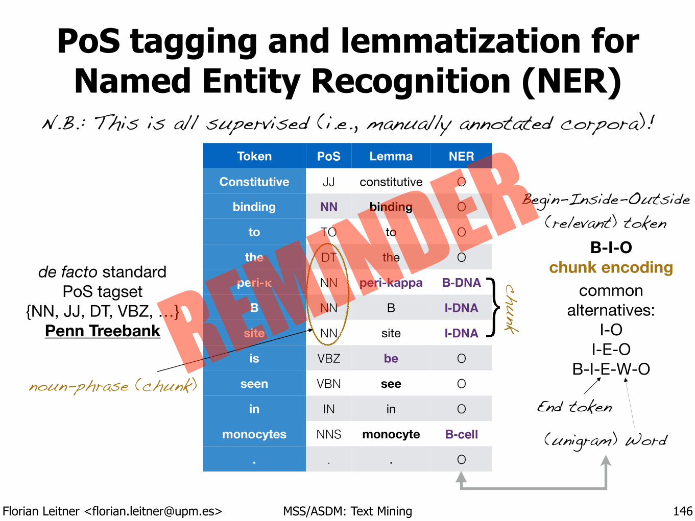
Florian Leitner <[email protected]> MSS/ASDM: Text Mining
PoS tagging and lemmatization forNamed Entity Recognition (NER)
146
Token PoS Lemma NER
Constitutive JJ constitutive O
binding NN binding O
to TO to O
the DT the O
peri-! NN peri-kappa B-DNA
B NN B I-DNA
site NN site I-DNA
is VBZ be O
seen VBN see O
in IN in O
monocytes NNS monocyte B-cell
. . . O
de facto standard PoS tagset
{NN, JJ, DT, VBZ, …}Penn Treebank
B-I-O chunk encoding
commonalternatives:
I-OI-E-O
B-I-E-W-O
End token
(unigram) Word
Begin-Inside-Outside (relevant) token
} chunk
noun-phrase (chunk)
N.B.: This is all supervised (i.e., manually annotated corpora)!
REMINDER
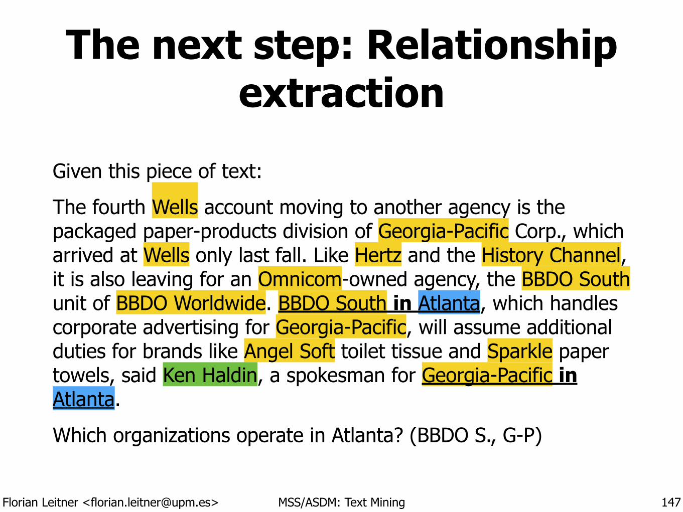
Florian Leitner <[email protected]> MSS/ASDM: Text Mining
The next step: Relationship extraction
Given this piece of text:
The fourth Wells account moving to another agency is the packaged paper-products division of Georgia-Pacific Corp., which arrived at Wells only last fall. Like Hertz and the History Channel, it is also leaving for an Omnicom-owned agency, the BBDO South unit of BBDO Worldwide. BBDO South in Atlanta, which handles corporate advertising for Georgia-Pacific, will assume additional duties for brands like Angel Soft toilet tissue and Sparkle paper towels, said Ken Haldin, a spokesman for Georgia-Pacific in Atlanta.
Which organizations operate in Atlanta? (BBDO S., G-P)
147
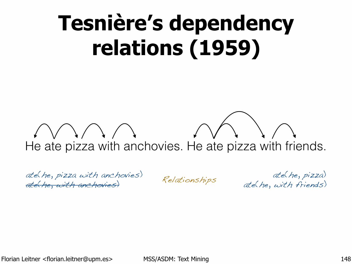
Florian Leitner <[email protected]> MSS/ASDM: Text Mining
Tesnière’s dependency relations (1959)
148
He ate pizza with anchovies. He ate pizza with friends.
ate(he, pizza with anchovies) ate(he, pizza)ate(he, with friends)Relationshipsate(he, with anchovies)
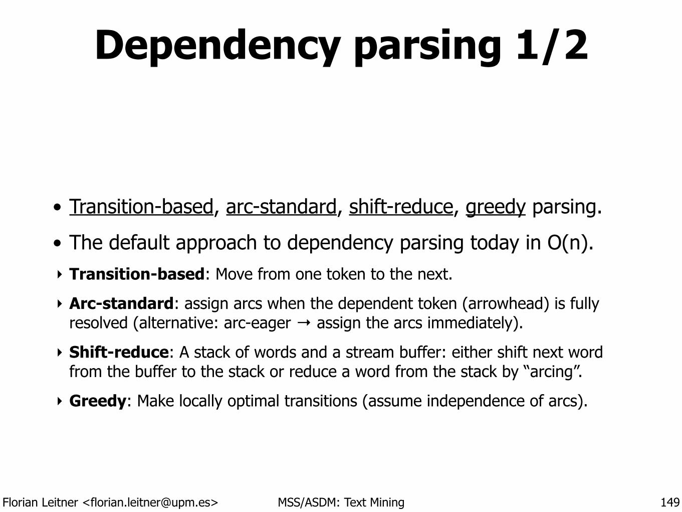
Florian Leitner <[email protected]> MSS/ASDM: Text Mining
Dependency parsing 1/2
• Transition-based, arc-standard, shift-reduce, greedy parsing.
• The default approach to dependency parsing today in O(n). ‣ Transition-based: Move from one token to the next.
‣ Arc-standard: assign arcs when the dependent token (arrowhead) is fully resolved (alternative: arc-eager → assign the arcs immediately).
‣ Shift-reduce: A stack of words and a stream buffer: either shift next word from the buffer to the stack or reduce a word from the stack by “arcing”.
‣ Greedy: Make locally optimal transitions (assume independence of arcs).
149
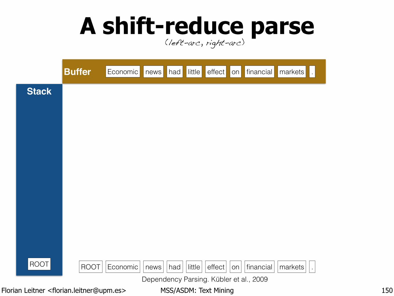
Florian Leitner <[email protected]> MSS/ASDM: Text Mining
Buffer
A shift-reduce parse
Stack
150
ROOT
Economic marketsfinancialoneffectlittlenews had .
ROOT Economic marketsfinancialoneffectlittlenews had .
(left-arc, right-arc)
Dependency Parsing. Kübler et al., 2009
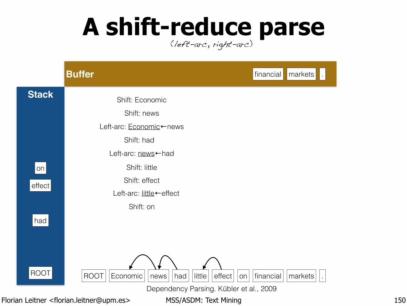
Florian Leitner <[email protected]> MSS/ASDM: Text Mining
Buffer
A shift-reduce parse
Stack
150
ROOT
marketsfinancial .
ROOT Economic marketsfinancialoneffectlittlenews had .
Shift: Economic
Shift: news
Left-arc: Economic←news
Shift: had
Left-arc: news←had
Shift: littleShift: effect
Left-arc: little←effect
had
effect
on
Shift: on
(left-arc, right-arc)
Dependency Parsing. Kübler et al., 2009
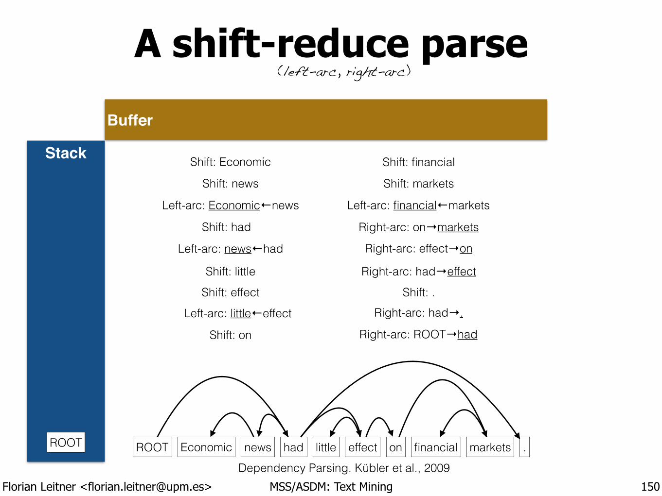
Florian Leitner <[email protected]> MSS/ASDM: Text Mining
Buffer
A shift-reduce parse
Stack
150
ROOT ROOT Economic marketsfinancialoneffectlittlenews had .
Shift: Economic
Shift: news
Left-arc: Economic←news
Shift: had
Left-arc: news←had
Shift: littleShift: effect
Left-arc: little←effect
Shift: on
Shift: financial
Shift: markets
Shift: .
Left-arc: financial←markets
Right-arc: on→marketsRight-arc: effect→on
Right-arc: had→effect
Right-arc: had→.
Right-arc: ROOT→had
(left-arc, right-arc)
Dependency Parsing. Kübler et al., 2009
Florian Leitner <[email protected]> MSS/ASDM: Text Mining
Dependency parsing 2/2
• (Arc-standard) Transitions: shift or reduce (left-arc, right-arc)
• Transitions are chosen using some classifier ‣ Maximum entropy classifier, support vector machine, single-layer perceptron,
perceptron with one hidden layer (→ Stanford parser, 2014 edition)
• Main issues: ‣ Few large, well annotated training corpora (“dependency treebanks”).
Biomedical domain: GENIA; Newswire: WSJ, Prague, Penn, …
‣ Non-projective trees (i.e., trees with arcs crossing each other; common in a number of other languages) with arcs that have to be drawn between nodes that are not adjacent on the stack.
151
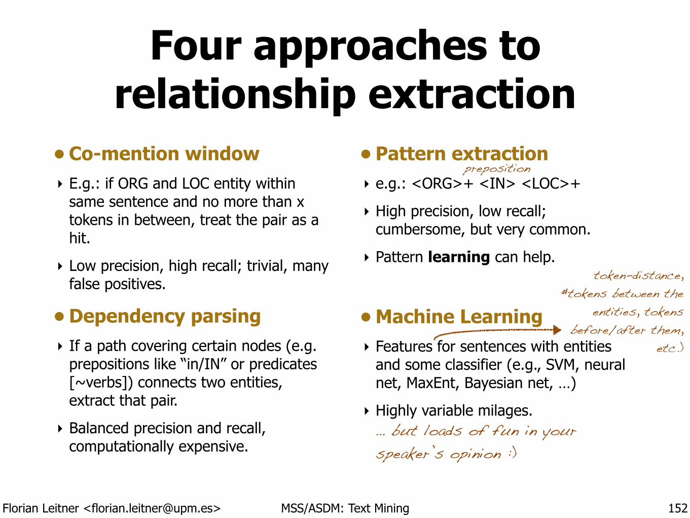
Florian Leitner <[email protected]> MSS/ASDM: Text Mining
Four approaches to relationship extraction
• Co-mention window ‣ E.g.: if ORG and LOC entity within
same sentence and no more than x tokens in between, treat the pair as a hit.
‣ Low precision, high recall; trivial, many false positives.
• Dependency parsing ‣ If a path covering certain nodes (e.g.
prepositions like “in/IN” or predicates [~verbs]) connects two entities, extract that pair.
‣ Balanced precision and recall, computationally expensive.
• Pattern extraction ‣ e.g.: <ORG>+ <IN> <LOC>+
‣ High precision, low recall; cumbersome, but very common.
‣ Pattern learning can help.
!
• Machine Learning ‣ Features for sentences with entities
and some classifier (e.g., SVM, neural net, MaxEnt, Bayesian net, …)
‣ Highly variable milages.… but loads of fun in your speaker’s opinion :)
152
preposition
token-distance, #tokens between the
entities, tokens before/after them,
etc.)
![Bare-Bones Dependency Parsing - Uppsala Universitystp.lingfil.uu.se/~nivre/docs/BareBones.pdf · I Parsing methods for bare-bones dependency parsing I Chart parsing ... Eisner 2000]:](https://img.pdfslide.us/doc/110x75/5b1dbccd7f8b9a397f8b5558/bare-bones-dependency-parsing-uppsala-nivredocsbarebonespdf-i-parsing-methods.jpg)


![Statistical Dependency Parsing - Uppsala Universitynivre/docs/StatState.pdf · I Methods for statistical dependency parsing I Chart parsing techniques ... Eisner 2000]: I Split head](https://img.pdfslide.us/doc/110x75/5b1dbccd7f8b9a397f8b5551/statistical-dependency-parsing-uppsala-university-nivredocsstatstatepdf.jpg)