Embed Size (px)
Citation preview
ANDREA MIGNONE
DIPARTIMENTO DI F IS ICA
UNIVERSITÀ DI TORINO ( ITALY)
Basic Discretization Methods in
Astrophysical Fluid Dynamics
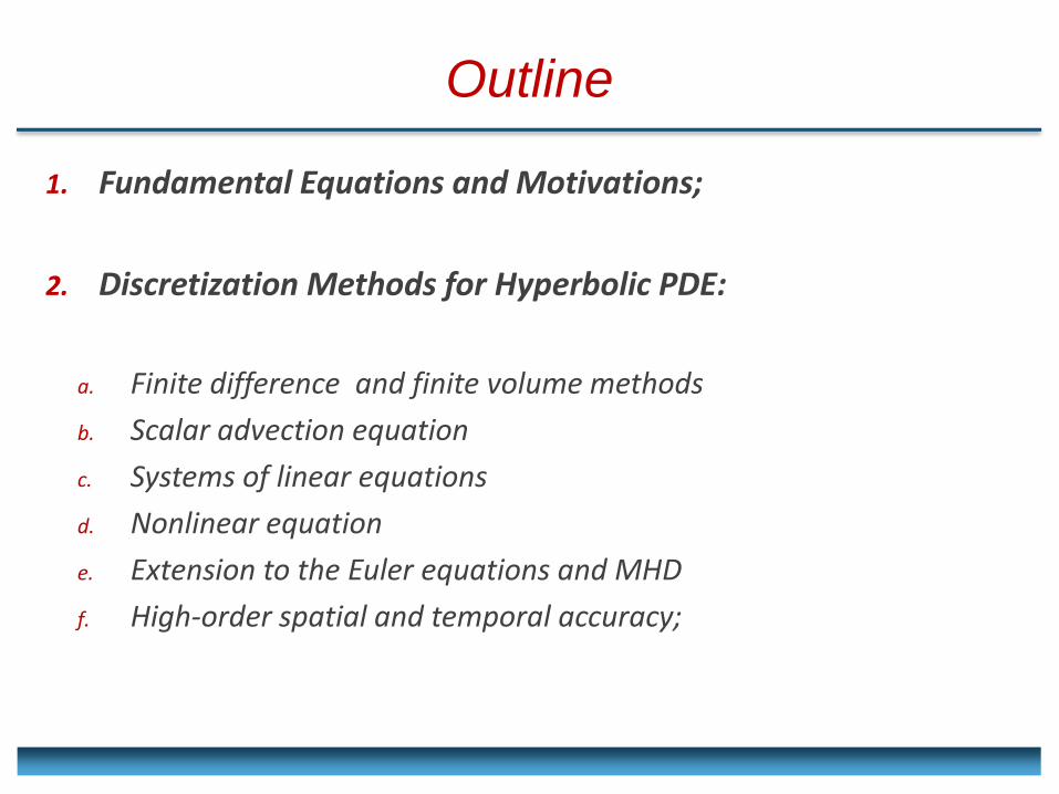
Outline
1. Fundamental Equations and Motivations;
2. Discretization Methods for Hyperbolic PDE:
a. Finite difference and finite volume methods
b. Scalar advection equation
c. Systems of linear equations
d. Nonlinear equation
e. Extension to the Euler equations and MHD
f. High-order spatial and temporal accuracy;
1. INTRODUCTION
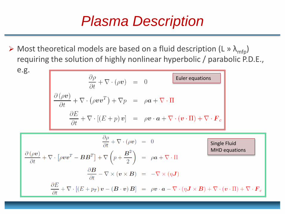
Most theoretical models are based on a fluid description (L » λmfp) requiring the solution of highly nonlinear hyperbolic / parabolic P.D.E., e.g.
Plasma Description
Euler equations
Single Fluid MHD equations
Exact solutions possible under very restrictive assumptions, e.g. stationarity (/t = 0), self-similarity, spherically symmetry or similar.
Nonlinear, time-dependent systems can be studied only by means of numerical simulations.
Grid-Based fluid approach via Finite Volume/Difference: Fluid variables are discretized on a spatial grid (static or adaptive) and evolved
in time.
Numerical solution of hyperbolic PDE in presence of discontinuous waves
Shock-Capturing (or Godunov-type) schemes.
Why Numerical Simulations ?
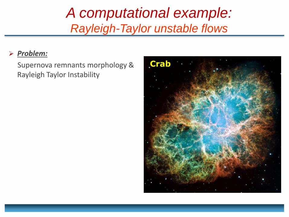
A computational example: Rayleigh-Taylor unstable flows
Problem:
Supernova remnants morphology & Rayleigh Taylor Instability
Crab
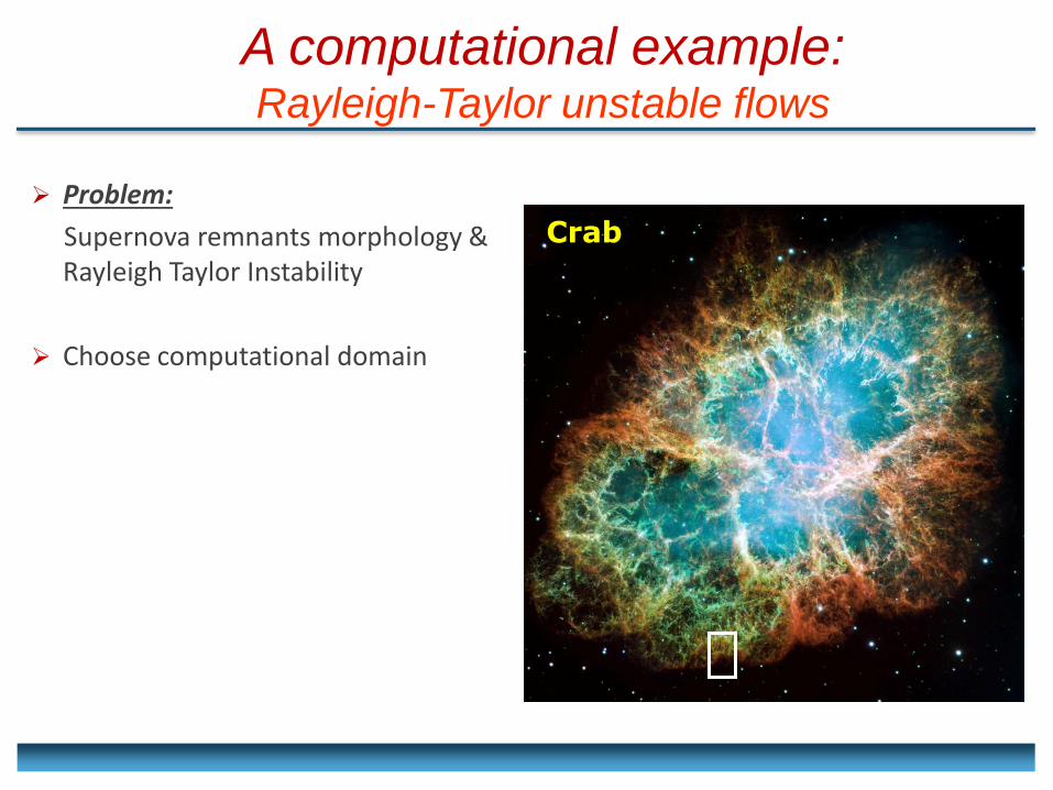
A computational example: Rayleigh-Taylor unstable flows
Problem:
Supernova remnants morphology & Rayleigh Taylor Instability
Choose computational domain
Crab
Lx ,Nx
Ly
Ny
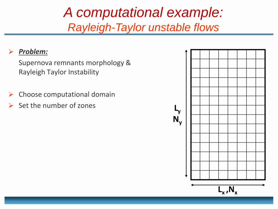
A computational example: Rayleigh-Taylor unstable flows
Problem:
Supernova remnants morphology & Rayleigh Taylor Instability
Choose computational domain
Set the number of zones
Lx ,Nx
Ly
Ny
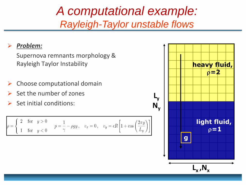
heavy fluid, =2
light fluid, =1
g
A computational example: Rayleigh-Taylor unstable flows
Problem:
Supernova remnants morphology & Rayleigh Taylor Instability
Choose computational domain
Set the number of zones
Set initial conditions:
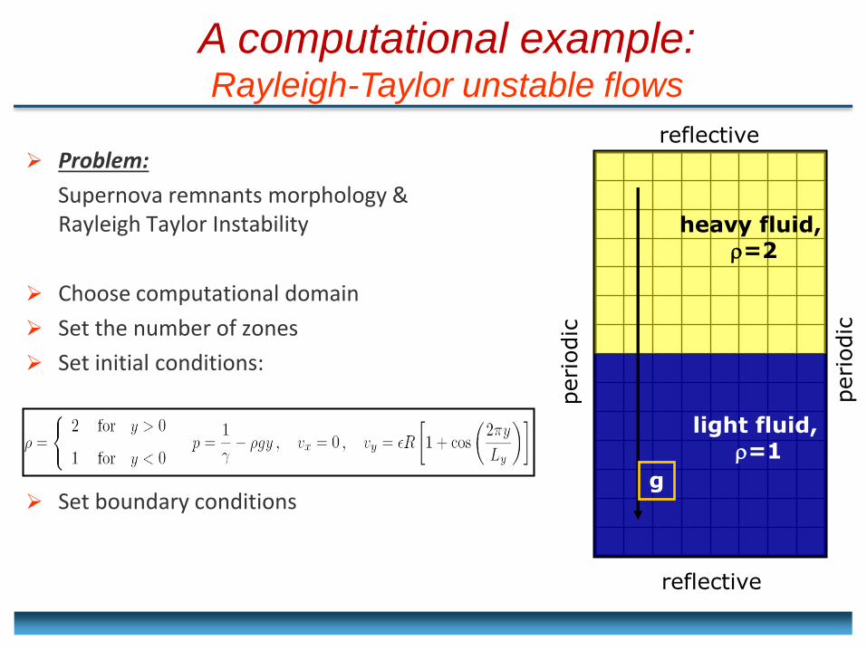
g
periodic
periodic
reflective
reflective
heavy fluid, =2
light fluid, =1
Problem:
Supernova remnants morphology & Rayleigh Taylor Instability
Choose computational domain
Set the number of zones
Set initial conditions:
Set boundary conditions
A computational example: Rayleigh-Taylor unstable flows
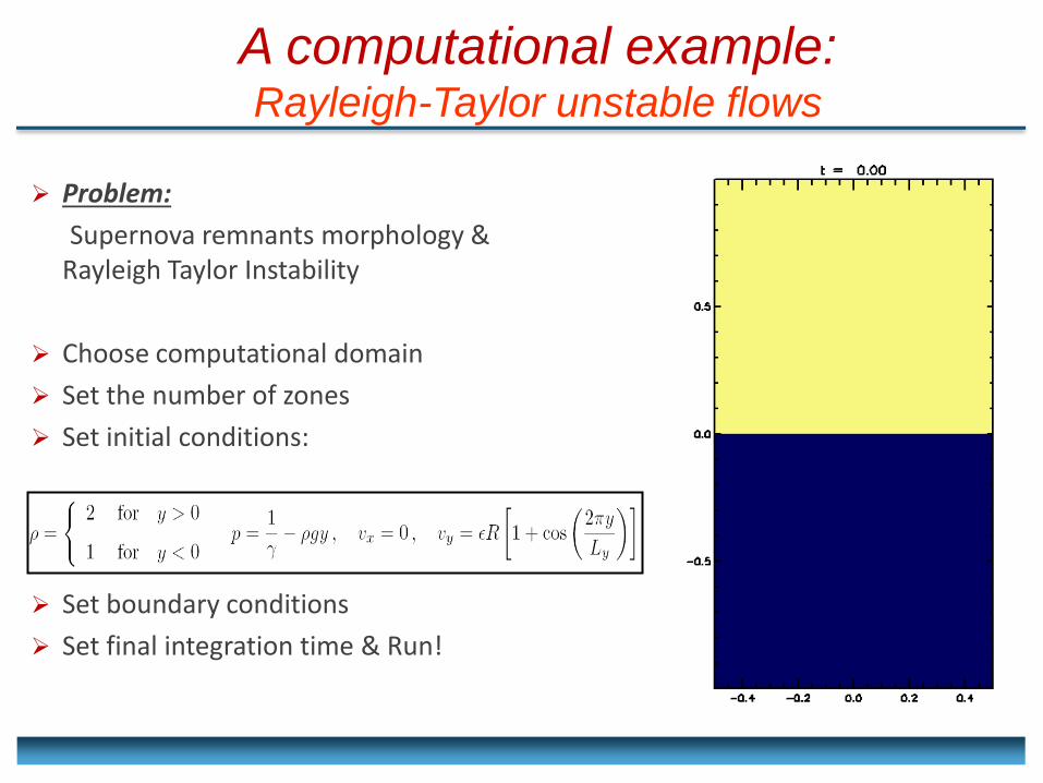
A computational example: Rayleigh-Taylor unstable flows
Problem:
Supernova remnants morphology & Rayleigh Taylor Instability
Choose computational domain
Set the number of zones
Set initial conditions:
Set boundary conditions
Set final integration time & Run!
F INITE DIFFERENCE
AND
F INITE VOLUME METHODS
2a. BASIC DISCRETIZATION METHODS FOR HYPERBOLIC PDE
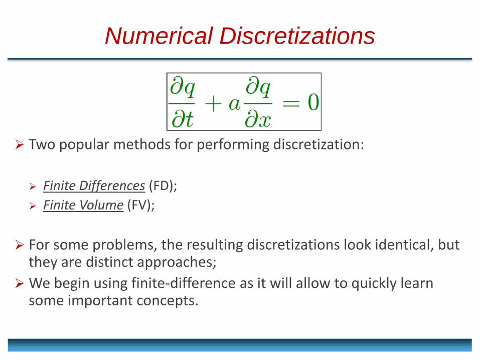
Numerical Discretizations
Two popular methods for performing discretization:
Finite Differences (FD);
Finite Volume (FV);
For some problems, the resulting discretizations look identical, but they are distinct approaches;
We begin using finite-difference as it will allow to quickly learn some important concepts.
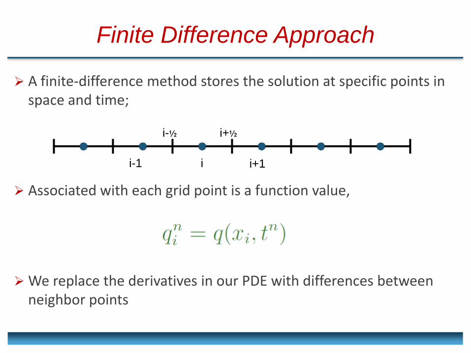
A finite-difference method stores the solution at specific points in space and time;
Associated with each grid point is a function value,
We replace the derivatives in our PDE with differences between neighbor points
Finite Difference Approach
i+1 i i-1
i+½ i-½
Finite Volume Approach
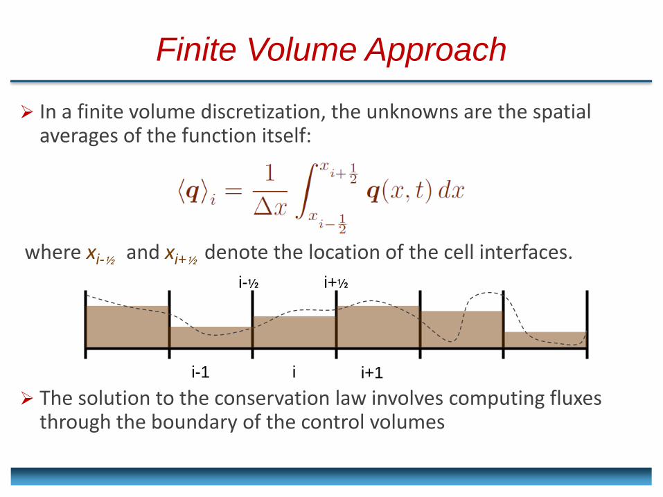
In a finite volume discretization, the unknowns are the spatial averages of the function itself:
where xi-½ and xi+½ denote the location of the cell interfaces.
The solution to the conservation law involves computing fluxes through the boundary of the control volumes
i+1 i i-1
i+½ i-½
Finite Volume Formulation
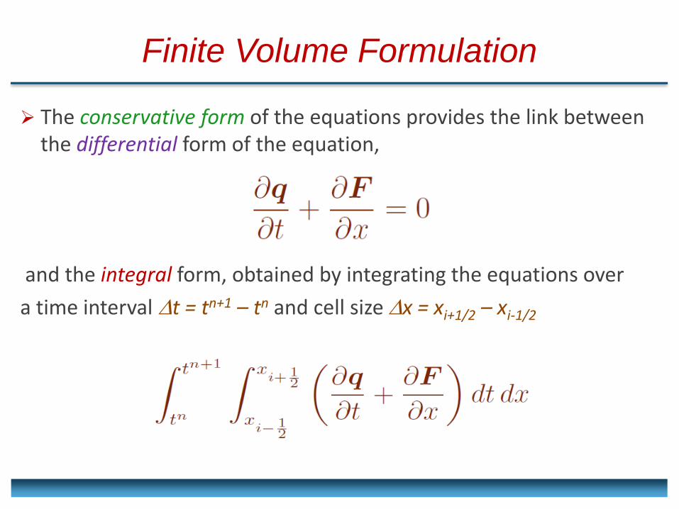
The conservative form of the equations provides the link between the differential form of the equation,
and the integral form, obtained by integrating the equations over
a time intervalt = tn+1 – tn and cell size x = xi+1/2 – xi-1/2
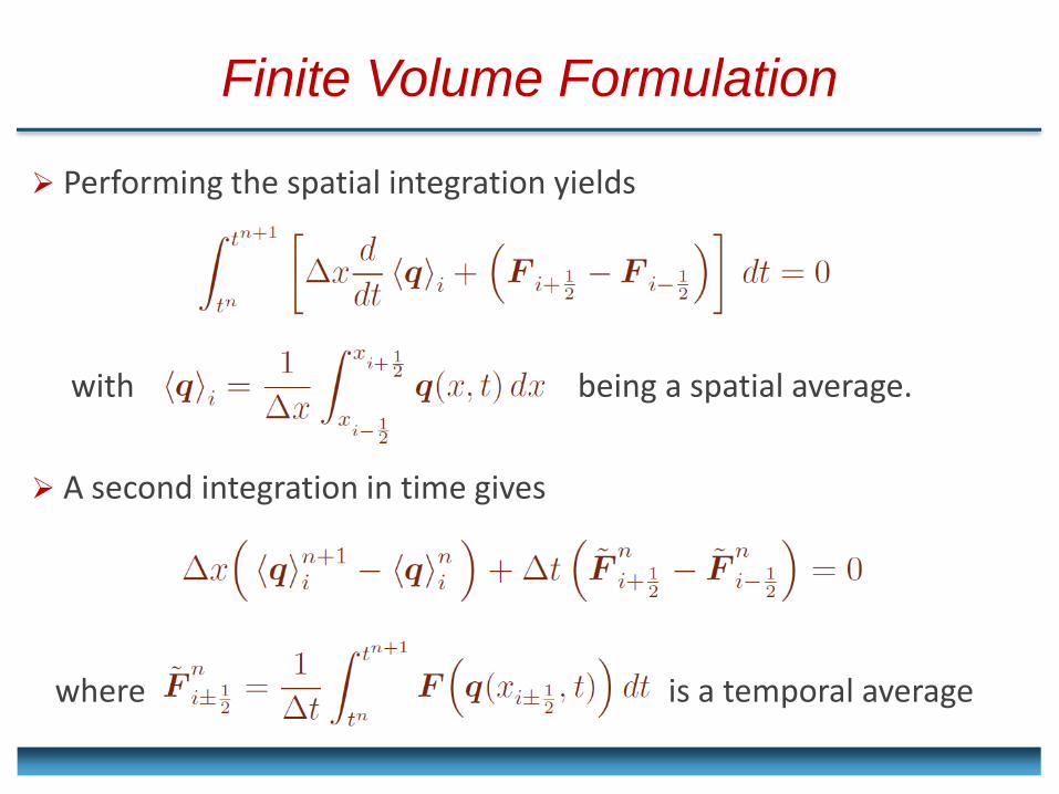
Performing the spatial integration yields
with being a spatial average.
A second integration in time gives
where is a temporal average
Finite Volume Formulation
Finite Volume Formulation
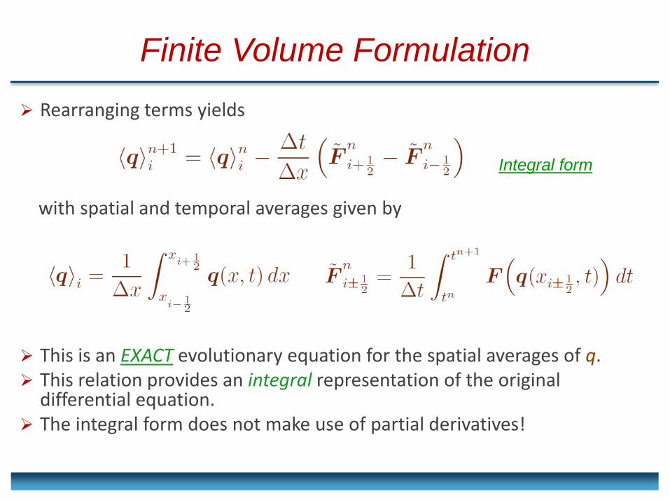
Rearranging terms yields
with spatial and temporal averages given by
This is an EXACT evolutionary equation for the spatial averages of q. This relation provides an integral representation of the original
differential equation. The integral form does not make use of partial derivatives!
Integral form
The Riemann Problem
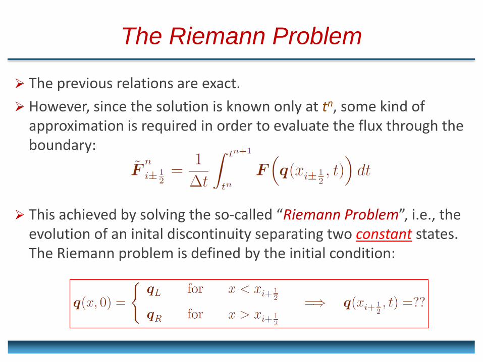
The previous relations are exact.
However, since the solution is known only at tn, some kind of approximation is required in order to evaluate the flux through the boundary:
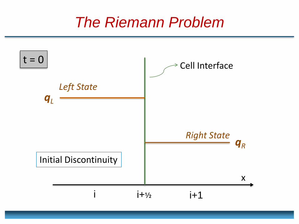
This achieved by solving the so-called “Riemann Problem”, i.e., the evolution of an inital discontinuity separating two constant states. The Riemann problem is defined by the initial condition:
The Riemann Problem
qL
qR
Left State
Right State
x
Cell Interface
i i+1 i+½
Initial Discontinuity
t = 0
The Riemann Problem
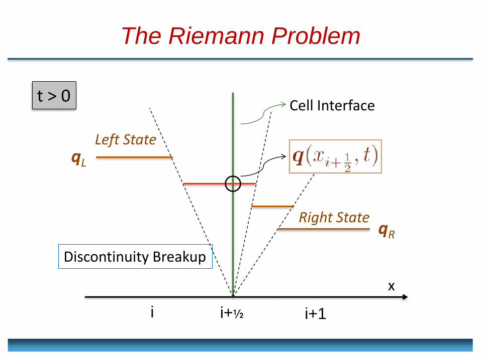
qL
qR
Left State
Right State
x
Cell Interface
i i+1 i+½
Discontinuity Breakup
t > 0
THE L INEAR SCALAR ADVECTION EQUATION
2b. BASIC DISCRETIZATION METHODS FOR HYPERBOLIC PDE
The Advection Equation: Theory
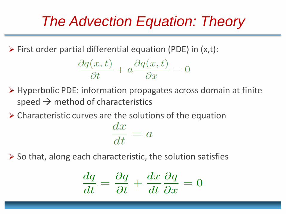
First order partial differential equation (PDE) in (x,t):
Hyperbolic PDE: information propagates across domain at finite speed method of characteristics
Characteristic curves are the solutions of the equation
So that, along each characteristic, the solution satisfies
The Advection Equation: Theory
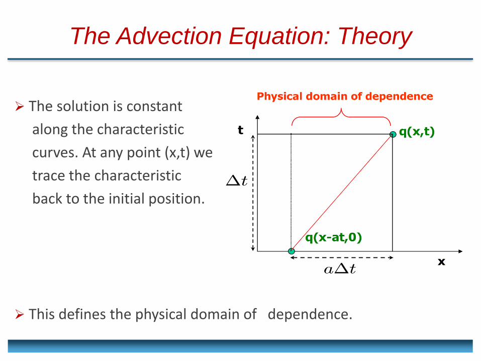
The solution is constant
along the characteristic
curves. At any point (x,t) we
trace the characteristic
back to the initial position.
This defines the physical domain of dependence.
The Advection Equation: Theory
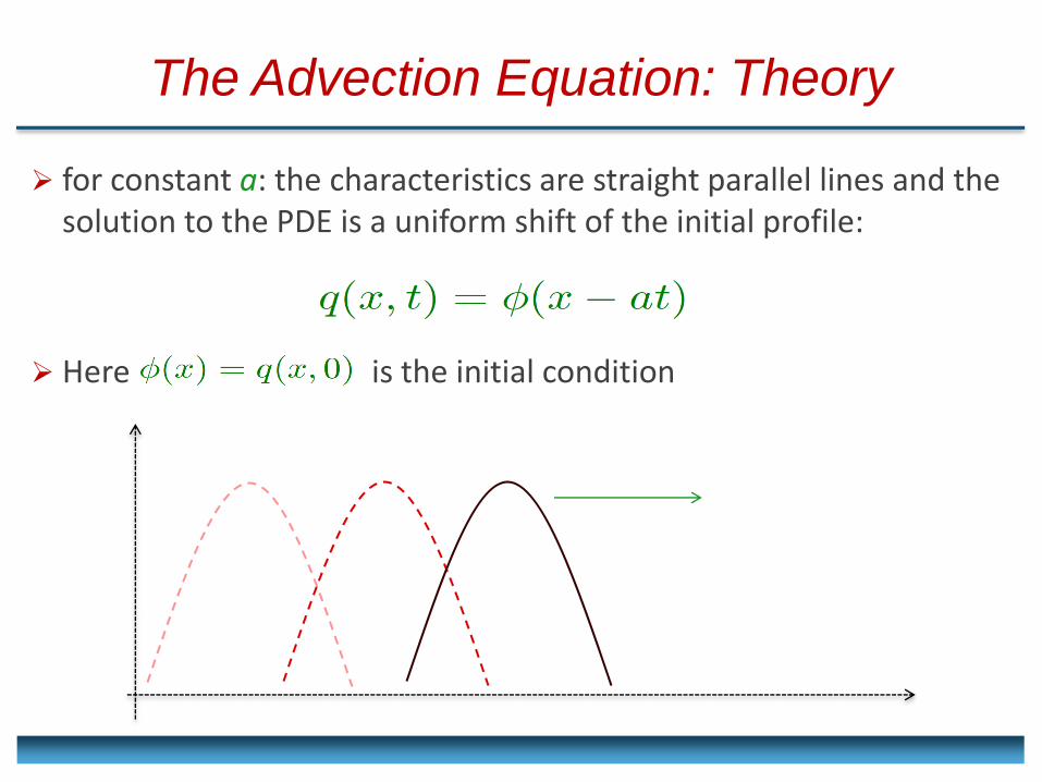
for constant a: the characteristics are straight parallel lines and the solution to the PDE is a uniform shift of the initial profile:
Here is the initial condition
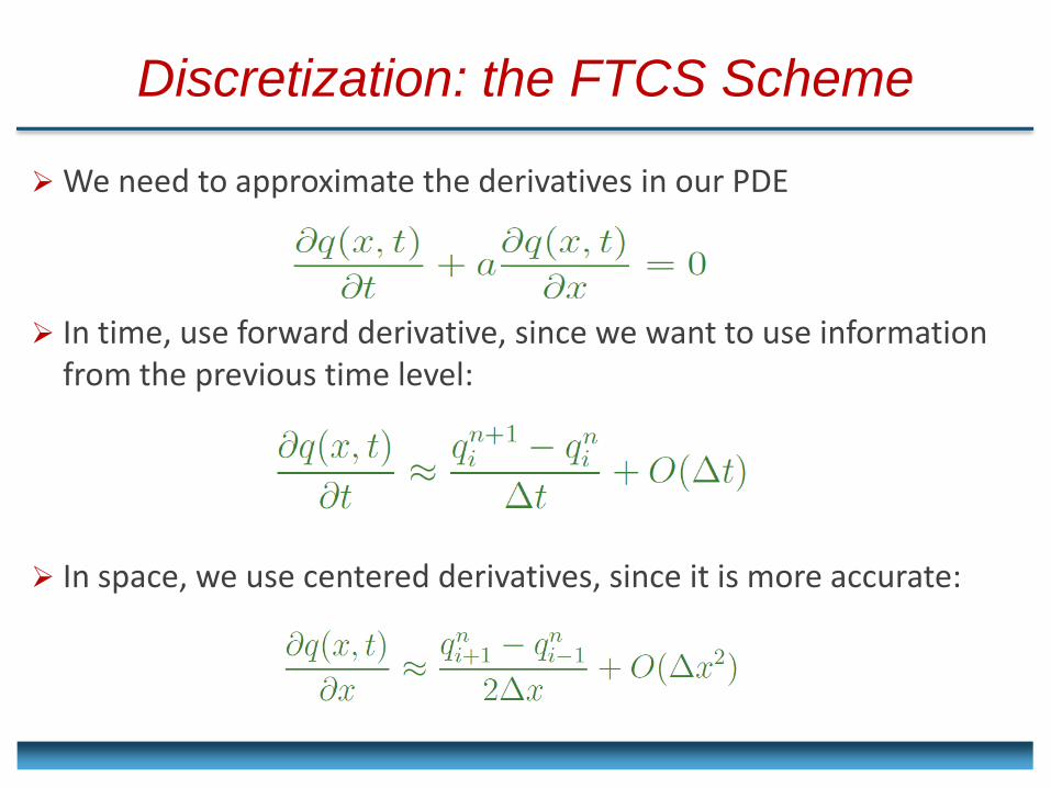
Discretization: the FTCS Scheme
We need to approximate the derivatives in our PDE
In time, use forward derivative, since we want to use information from the previous time level:
In space, we use centered derivatives, since it is more accurate:
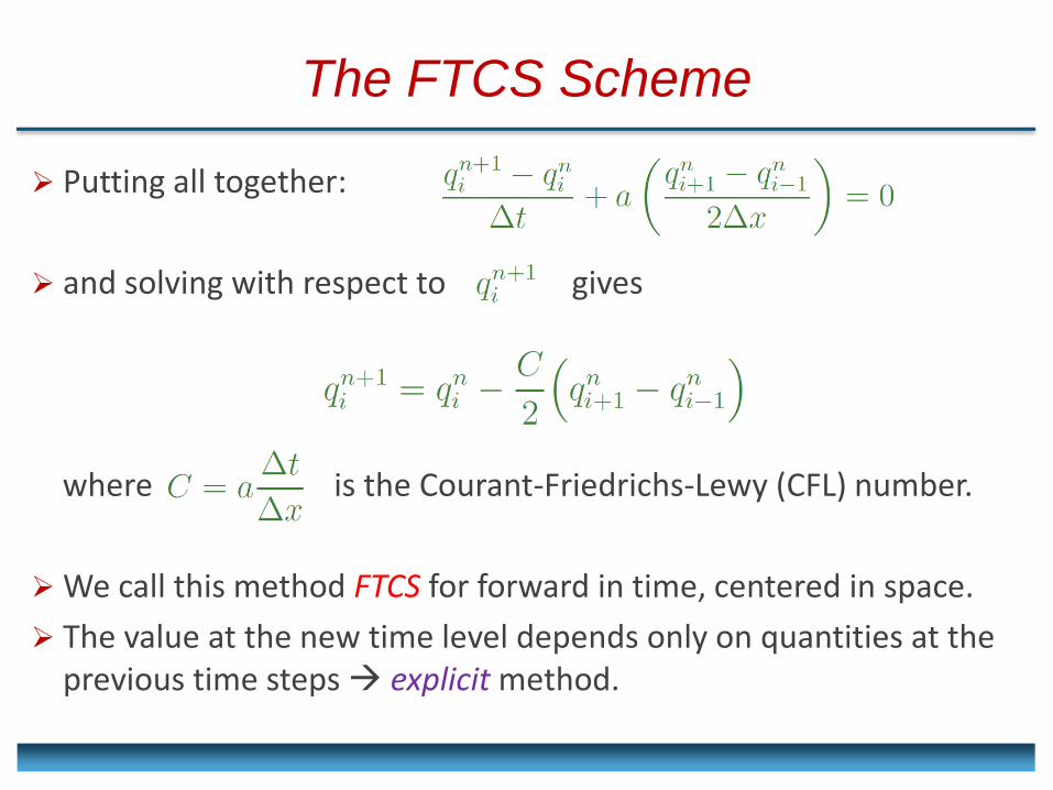
The FTCS Scheme
Putting all together:
and solving with respect to gives
where is the Courant-Friedrichs-Lewy (CFL) number.
We call this method FTCS for forward in time, centered in space.
The value at the new time level depends only on quantities at the previous time steps explicit method.
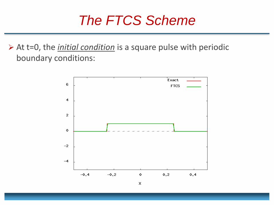
The FTCS Scheme
At t=0, the initial condition is a square pulse with periodic boundary conditions:
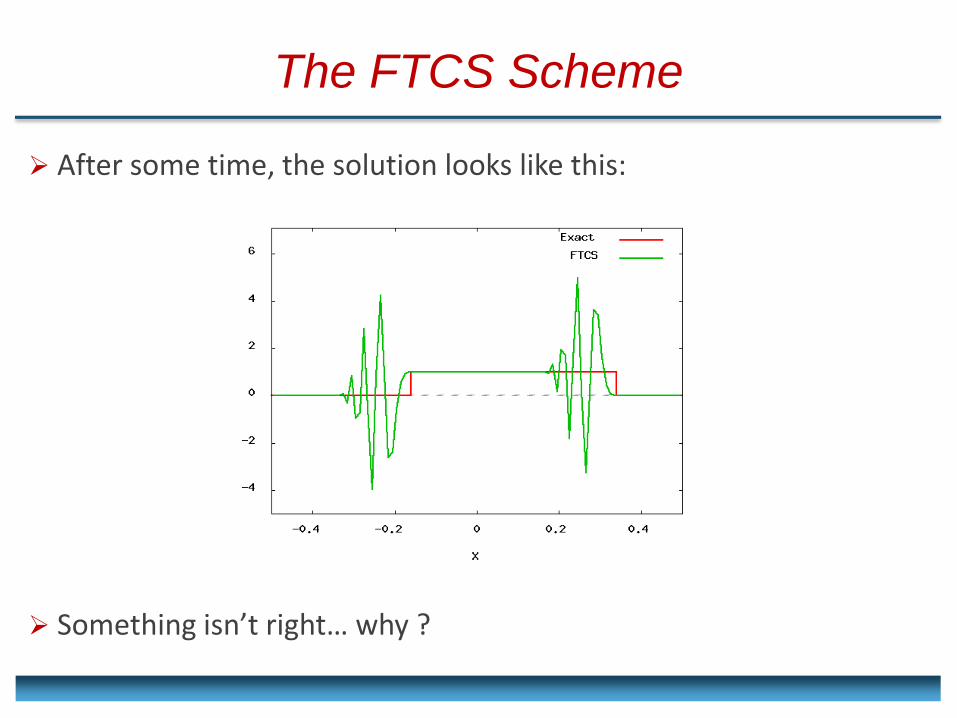
The FTCS Scheme
After some time, the solution looks like this:
Something isn’t right… why ?
von Neumann Stability Analysis
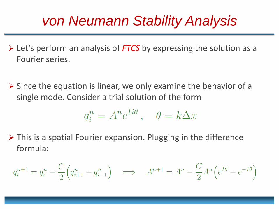
Let’s perform an analysis of FTCS by expressing the solution as a Fourier series.
Since the equation is linear, we only examine the behavior of a single mode. Consider a trial solution of the form
This is a spatial Fourier expansion. Plugging in the difference formula:
von Neumann Stability Analysis
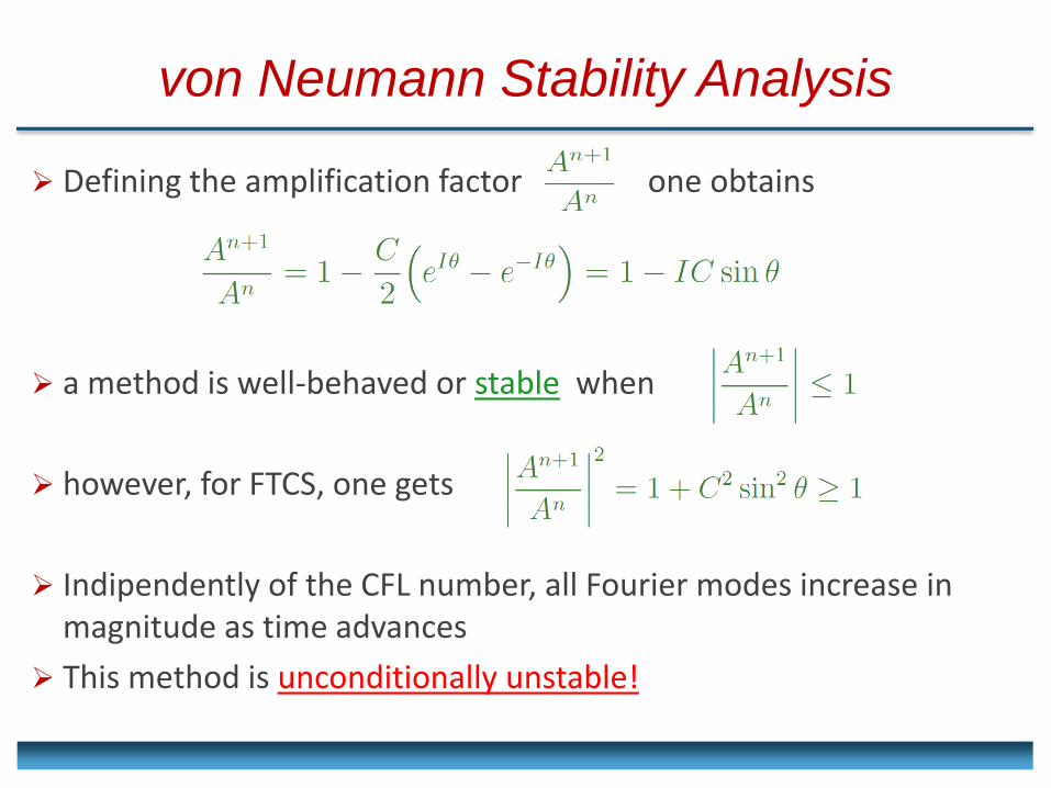
Defining the amplification factor one obtains
a method is well-behaved or stable when
however, for FTCS, one gets
Indipendently of the CFL number, all Fourier modes increase in magnitude as time advances
This method is unconditionally unstable!
Forward in Time, Backward in Space
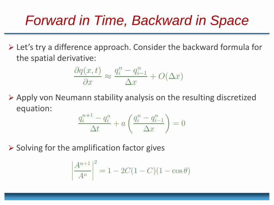
Let’s try a difference approach. Consider the backward formula for the spatial derivative:
Apply von Neumann stability analysis on the resulting discretized equation:
Solving for the amplification factor gives
Forward in Time, Backward in Space
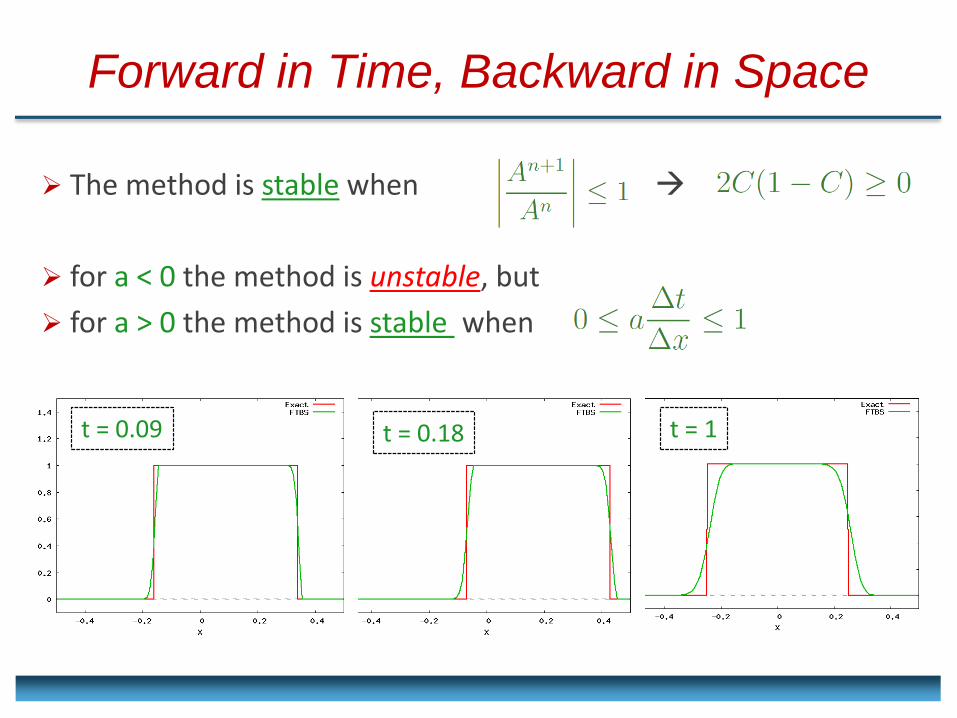
The method is stable when
for a < 0 the method is unstable, but
for a > 0 the method is stable when
t = 0.09 t = 0.18 t = 1
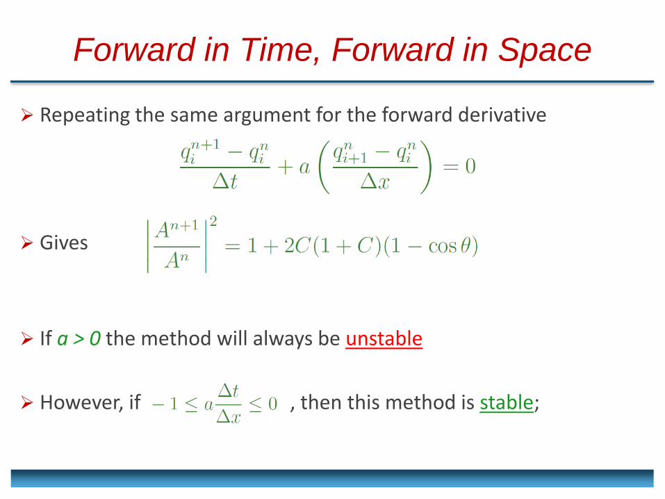
Forward in Time, Forward in Space
Repeating the same argument for the forward derivative
Gives
If a > 0 the method will always be unstable
However, if , then this method is stable;
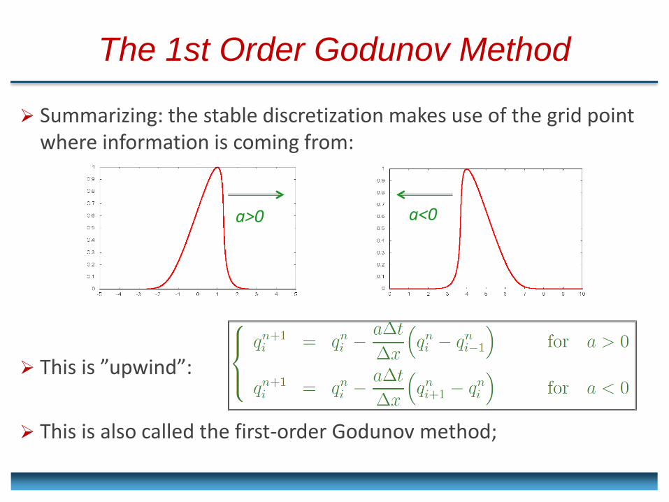
Summarizing: the stable discretization makes use of the grid point where information is coming from:
This is ”upwind”:
This is also called the first-order Godunov method;
The 1st Order Godunov Method
a>0 a<0
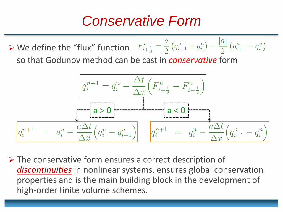
We define the “flux” function
so that Godunov method can be cast in conservative form
The conservative form ensures a correct description of discontinuities in nonlinear systems, ensures global conservation properties and is the main building block in the development of high-order finite volume schemes.
Conservative Form
a > 0 a < 0
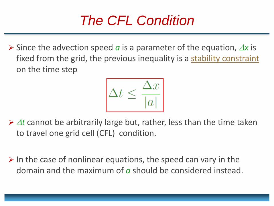
The CFL Condition
Since the advection speed a is a parameter of the equation, x is fixed from the grid, the previous inequality is a stability constraint on the time step
t cannot be arbitrarily large but, rather, less than the time taken to travel one grid cell (CFL) condition.
In the case of nonlinear equations, the speed can vary in the domain and the maximum of a should be considered instead.
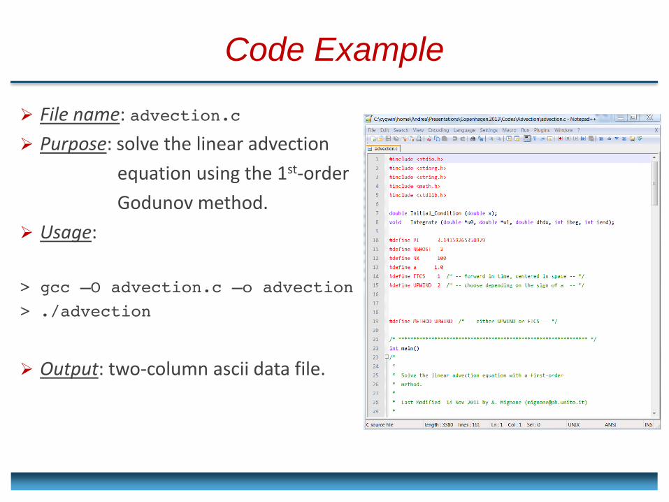
File name: advection.c
Purpose: solve the linear advection
equation using the 1st-order
Godunov method.
Usage:
> gcc –O advection.c –o advection
> ./advection
Output: two-column ascii data file.
Code Example
SYSTEM OF L INEAR EQUATIONS
2c. BASIC DISCRETIZATION METHODS FOR HYPERBOLIC PDE:
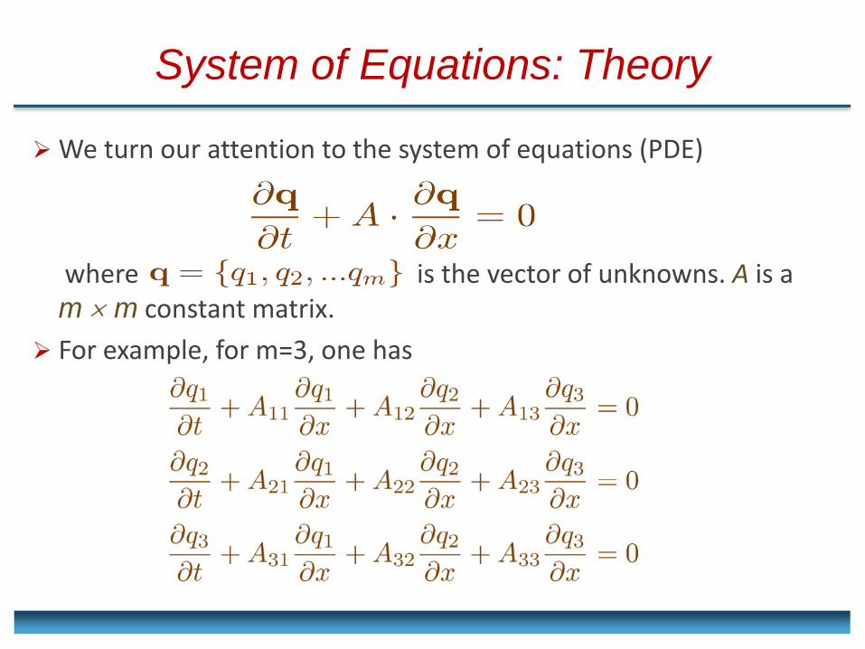
System of Equations: Theory
We turn our attention to the system of equations (PDE)
where is the vector of unknowns. A is a m m constant matrix.
For example, for m=3, one has
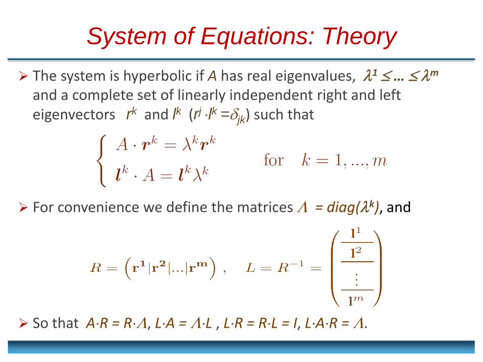
System of Equations: Theory
The system is hyperbolic if A has real eigenvalues, 1 … m and a complete set of linearly independent right and left eigenvectors rk and lk (rj lk =jk) such that
For convenience we define the matrices = diag(k), and
So that AR = R, LA = L , LR = RL = I, LAR = .
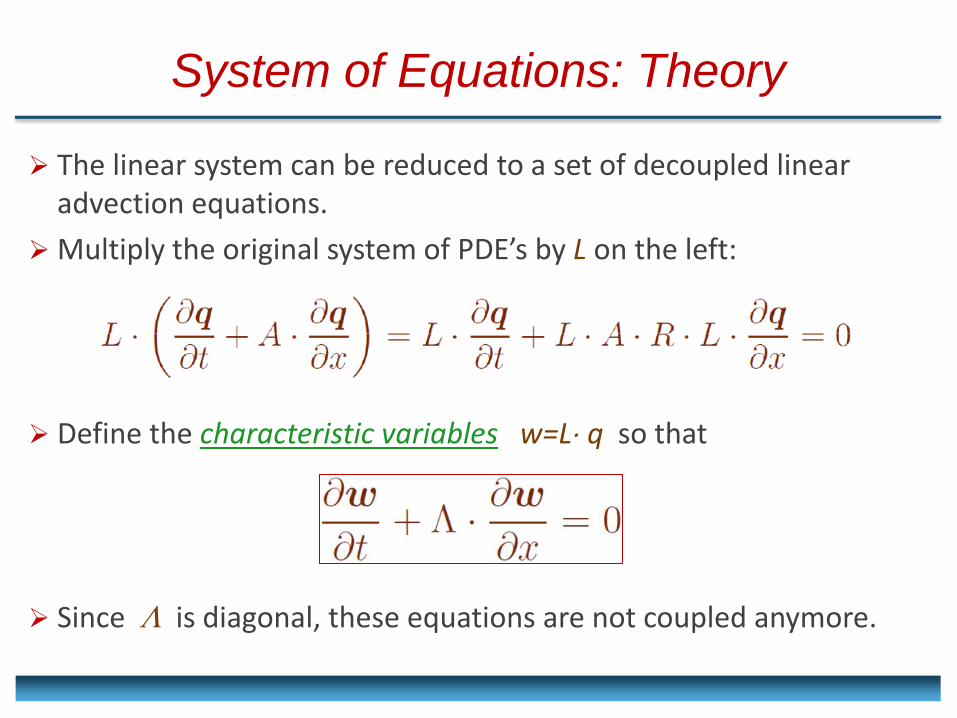
The linear system can be reduced to a set of decoupled linear advection equations.
Multiply the original system of PDE’s by L on the left:
Define the characteristic variables w=L q so that
Since is diagonal, these equations are not coupled anymore.
System of Equations: Theory
System of Equations: Theory
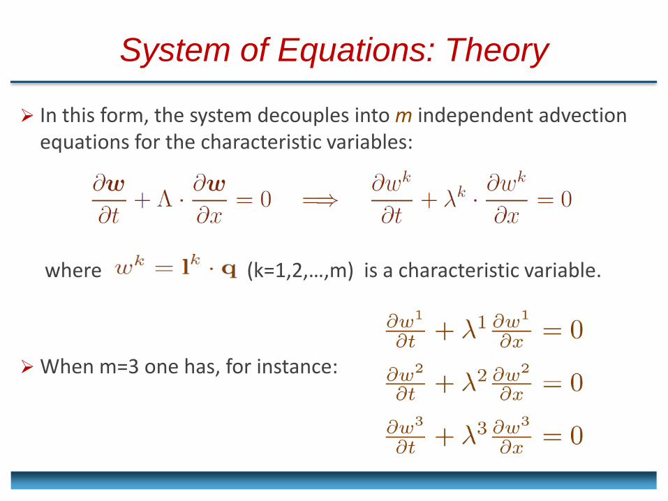
In this form, the system decouples into m independent advection equations for the characteristic variables:
where (k=1,2,…,m) is a characteristic variable.
When m=3 one has, for instance:
System of Equations: Theory
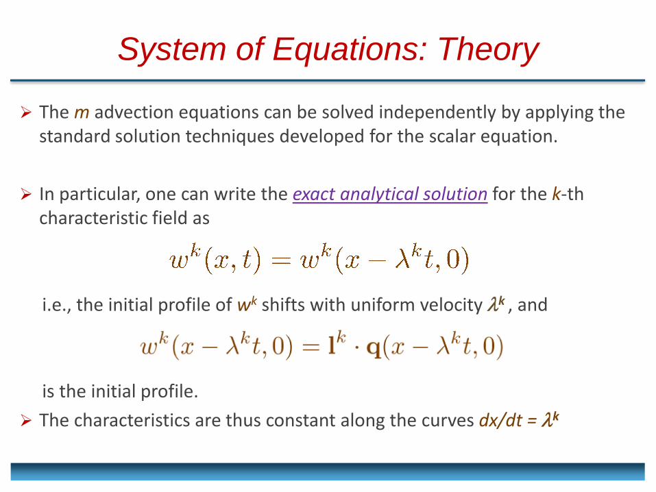
The m advection equations can be solved independently by applying the standard solution techniques developed for the scalar equation.
In particular, one can write the exact analytical solution for the k-th characteristic field as
i.e., the initial profile of wk shifts with uniform velocity k , and
is the initial profile.
The characteristics are thus constant along the curves dx/dt = k
System of Equations: Exact Solution
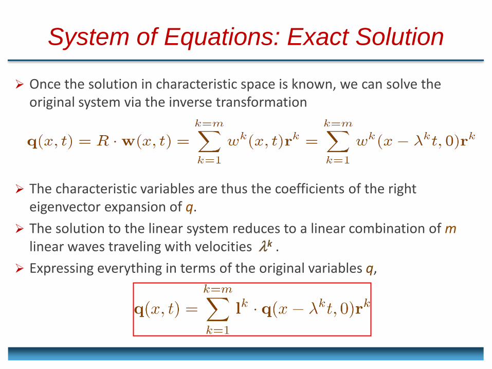
Once the solution in characteristic space is known, we can solve the original system via the inverse transformation
The characteristic variables are thus the coefficients of the right eigenvector expansion of q.
The solution to the linear system reduces to a linear combination of m linear waves traveling with velocities k .
Expressing everything in terms of the original variables q,
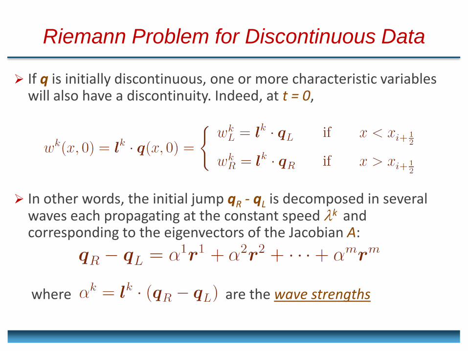
Riemann Problem for Discontinuous Data
If q is initially discontinuous, one or more characteristic variables will also have a discontinuity. Indeed, at t = 0,
In other words, the initial jump qR - qL is decomposed in several waves each propagating at the constant speed k and corresponding to the eigenvectors of the Jacobian A:
where are the wave strengths
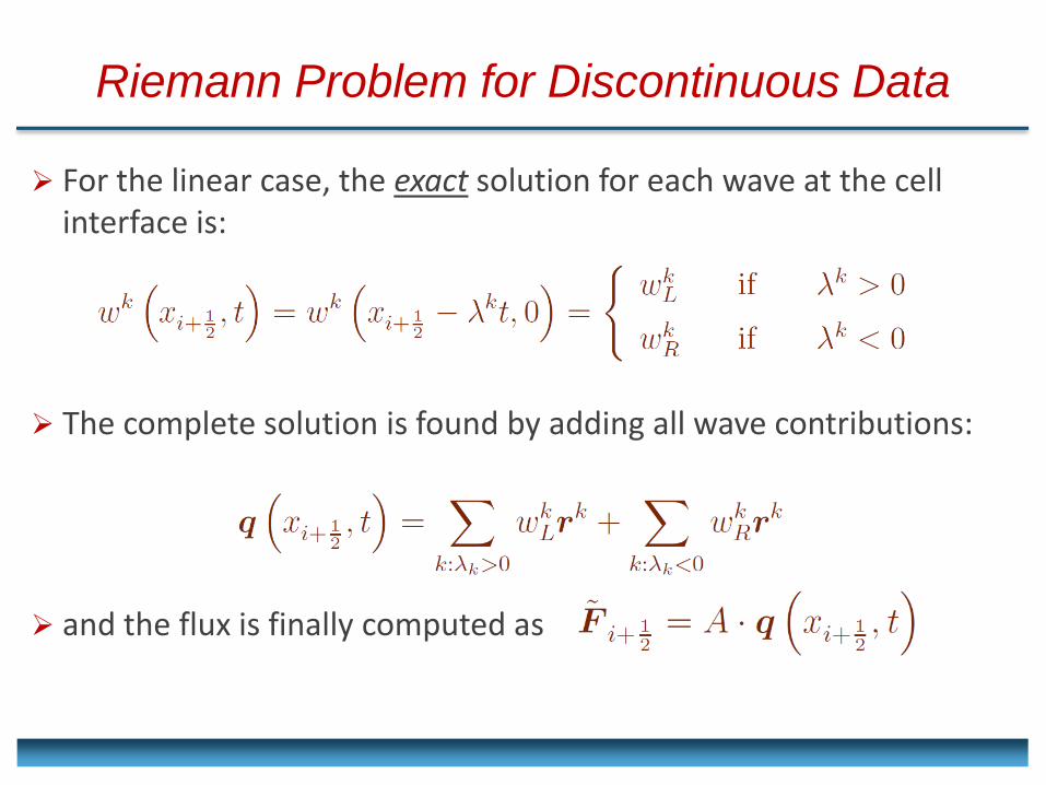
Riemann Problem for Discontinuous Data
For the linear case, the exact solution for each wave at the cell interface is:
The complete solution is found by adding all wave contributions:
and the flux is finally computed as
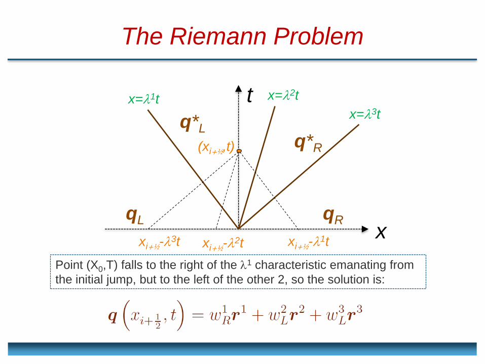
The Riemann Problem
qL qR
q*L
q*R
x=1t x=2t
x=3t
x
t
xi+½-2t
(xi+½,t)
xi+½-3t xi+½-1t
Point (X0,T) falls to the right of the 1 characteristic emanating from
the initial jump, but to the left of the other 2, so the solution is:
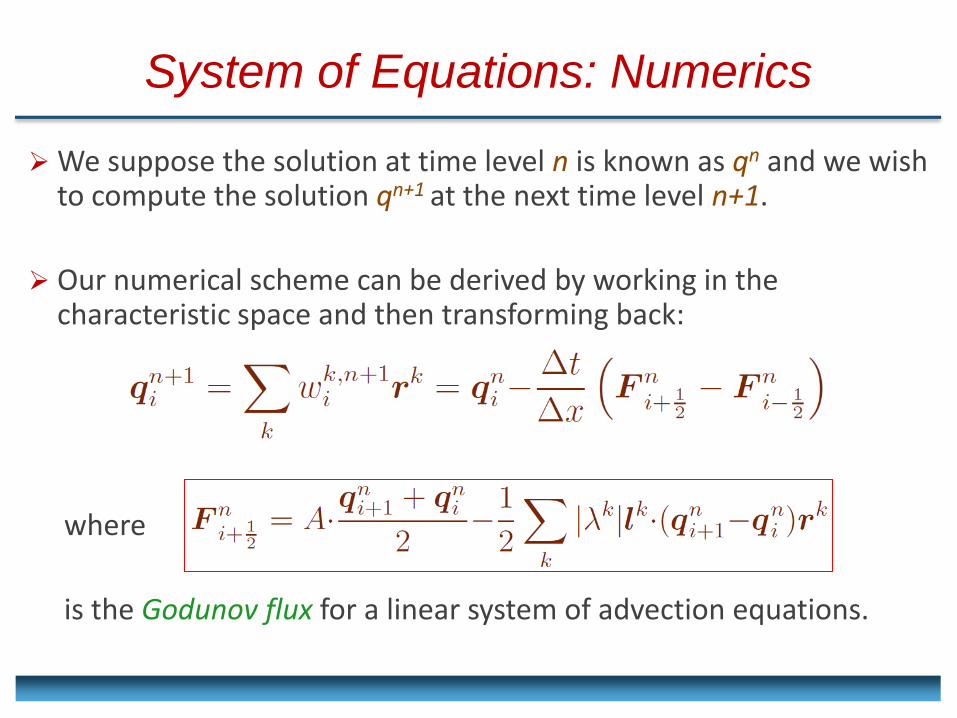
System of Equations: Numerics
We suppose the solution at time level n is known as qn and we wish to compute the solution qn+1 at the next time level n+1.
Our numerical scheme can be derived by working in the characteristic space and then transforming back:
where
is the Godunov flux for a linear system of advection equations.
NONLINEAR SCALAR EQUATION
2d. BASIC DISCRETIZATION METHODS FOR HYPERBOLIC PDE:
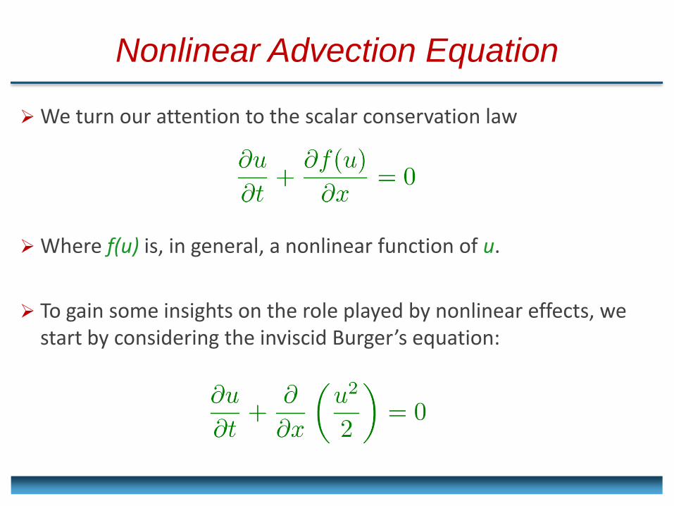
Nonlinear Advection Equation
We turn our attention to the scalar conservation law
Where f(u) is, in general, a nonlinear function of u.
To gain some insights on the role played by nonlinear effects, we start by considering the inviscid Burger’s equation:
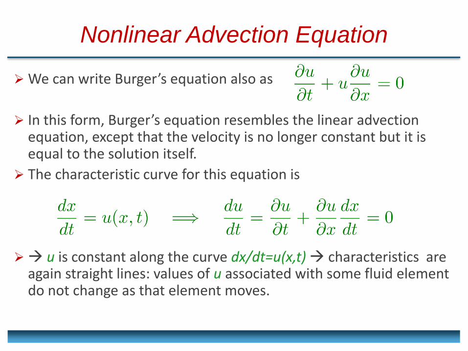
We can write Burger’s equation also as
In this form, Burger’s equation resembles the linear advection equation, except that the velocity is no longer constant but it is equal to the solution itself.
The characteristic curve for this equation is
u is constant along the curve dx/dt=u(x,t) characteristics are again straight lines: values of u associated with some fluid element do not change as that element moves.
Nonlinear Advection Equation
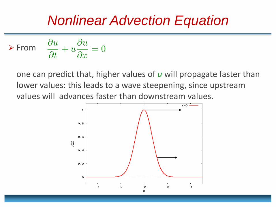
From
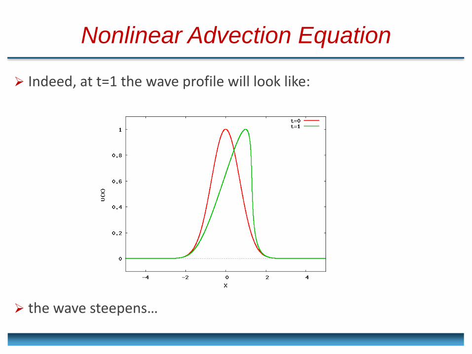
one can predict that, higher values of u will propagate faster than lower values: this leads to a wave steepening, since upstream values will advances faster than downstream values.
Nonlinear Advection Equation
Nonlinear Advection Equation
Indeed, at t=1 the wave profile will look like:
the wave steepens…
Nonlinear Advection Equation
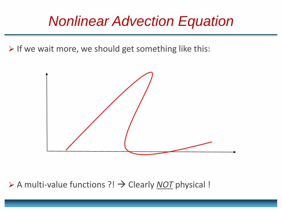
If we wait more, we should get something like this:
A multi-value functions ?! Clearly NOT physical !
Nonlinear Advection Equation
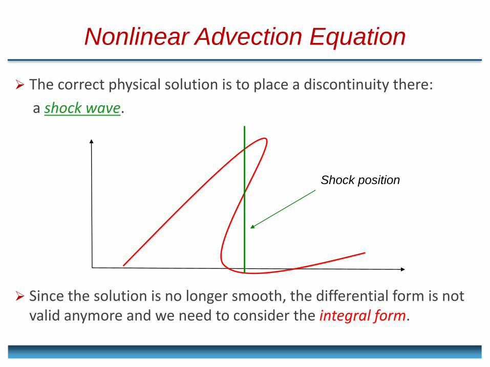
The correct physical solution is to place a discontinuity there:
a shock wave.
Since the solution is no longer smooth, the differential form is not valid anymore and we need to consider the integral form.
Shock position
Nonlinear Advection Equation
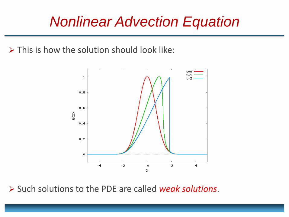
This is how the solution should look like:
Such solutions to the PDE are called weak solutions.
Nonlinear Advection Equation
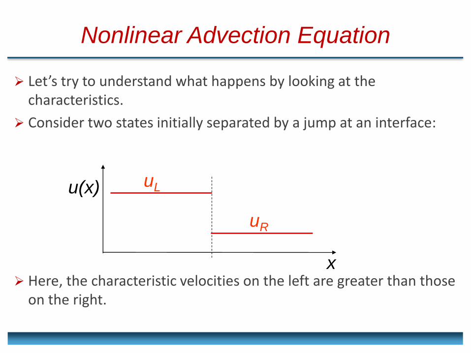
Let’s try to understand what happens by looking at the characteristics.
Consider two states initially separated by a jump at an interface:
Here, the characteristic velocities on the left are greater than those on the right.
uL
uR
u(x)
x
Nonlinear Advection Equation
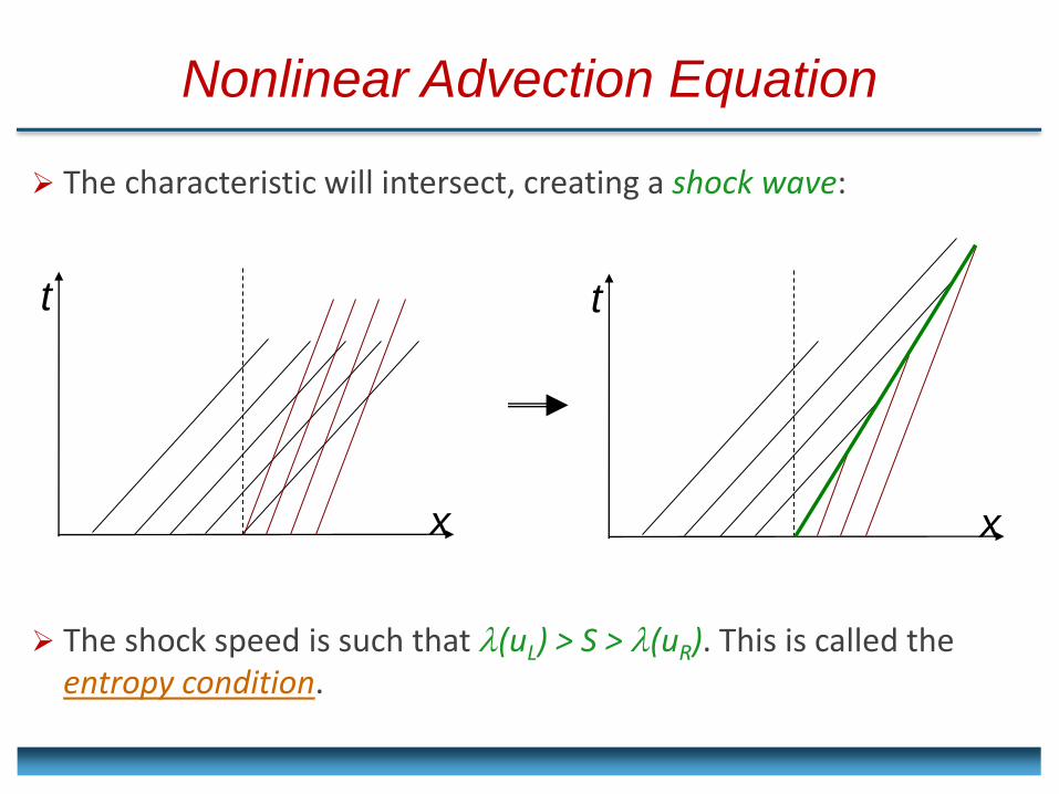
The characteristic will intersect, creating a shock wave:
The shock speed is such that (uL) > S > (uR). This is called the entropy condition.
t
x
t
x
Nonlinear Advection Equation
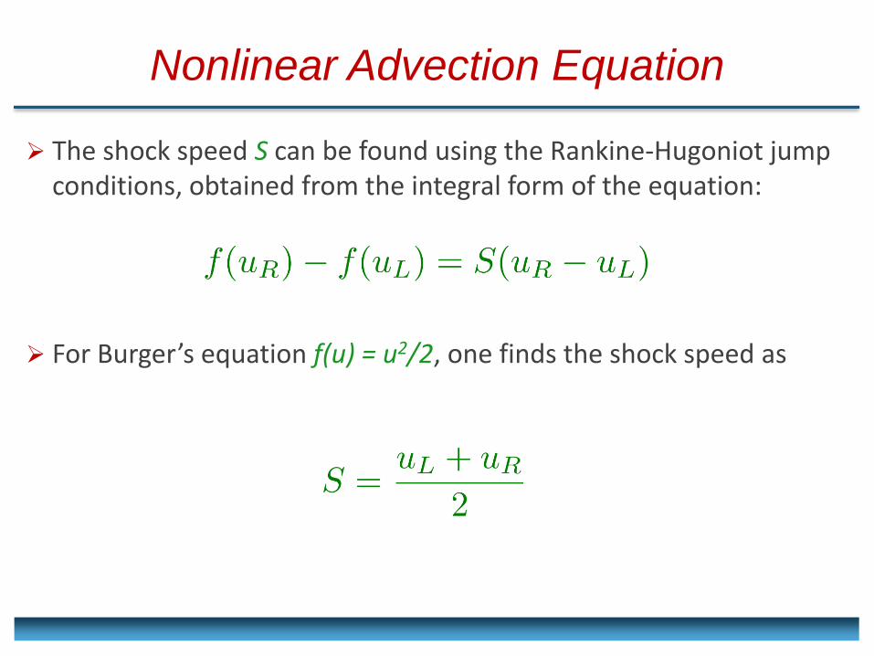
The shock speed S can be found using the Rankine-Hugoniot jump conditions, obtained from the integral form of the equation:
For Burger’s equation f(u) = u2/2, one finds the shock speed as
Nonlinear Advection Equation
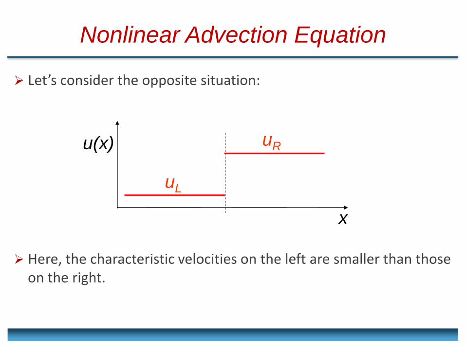
Let’s consider the opposite situation:
Here, the characteristic velocities on the left are smaller than those on the right.
uL
uR u(x)
x
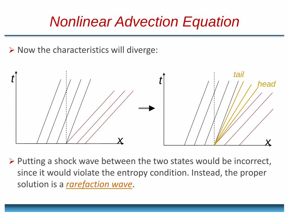
Nonlinear Advection Equation
Now the characteristics will diverge:
Putting a shock wave between the two states would be incorrect, since it would violate the entropy condition. Instead, the proper solution is a rarefaction wave.
t
x
t
x
tail
head
Nonlinear Advection Equation
A rarefaction wave is a nonlinear wave that smoothly connects the left and the right state. It is an expansion wave.
The solution between the states can only be self-similar and takes on the range of values between uL and uR
The head of the rarefaction moves at the speed (uR), whereas the tail moves at the speed (uL).
The general condition for a rarefaction wave is (uL)<(uR)
Both rarefactions and shocks are present in the solutions to the Euler equation. Both waves are nonlinear.
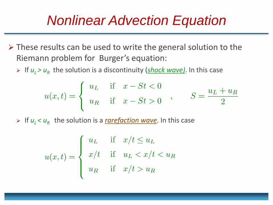
Nonlinear Advection Equation
These results can be used to write the general solution to the Riemann problem for Burger’s equation: If uL > uR the solution is a discontinuity (shock wave). In this case
If uL < uR the solution is a rarefaction wave. In this case
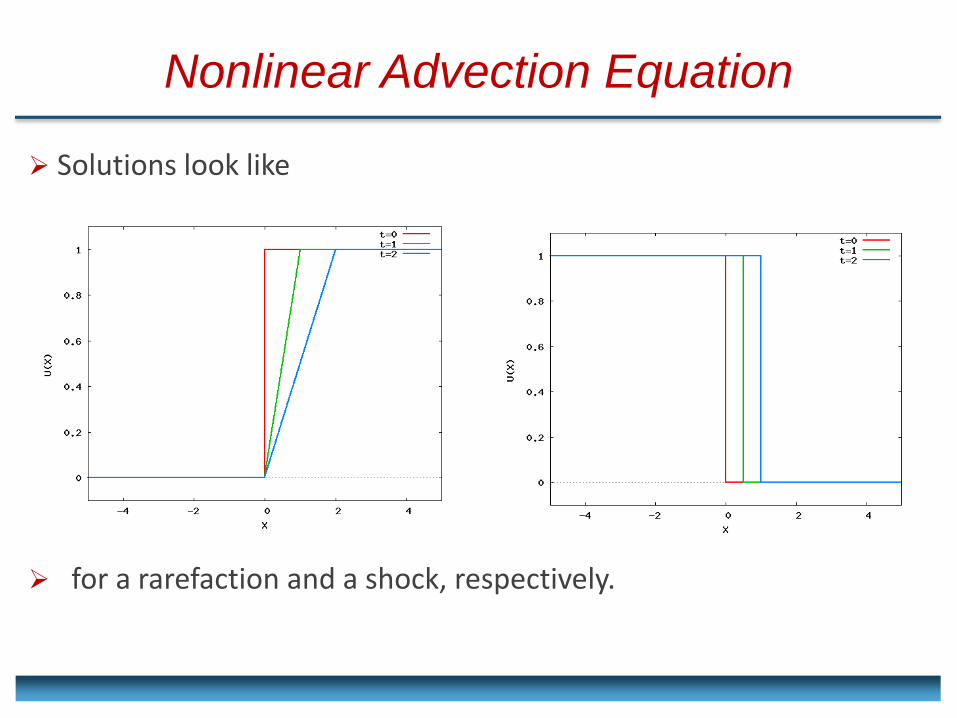
Nonlinear Advection Equation
Solutions look like
for a rarefaction and a shock, respectively.
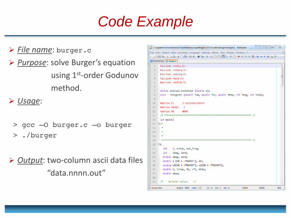
File name: burger.c
Purpose: solve Burger’s equation
using 1st-order Godunov
method.
Usage:
> gcc –O burger.c –o burger
> ./burger
Output: two-column ascii data files
“data.nnnn.out”
Code Example
NONLINEAR SYSTEMS
2e. BASIC DISCRETIZATION METHODS FOR HYPERBOLIC PDE:
Nonlinear Systems
Much of what is known about the numerical solution of hyperbolic systems of nonlinear equations comes from the results obtained in the linear case or simple nonlinear scalar equations.
The key idea is to exploit the conservative form and assume the system can be locally “frozen” at each grid interface.
However, this still requires the solution of the Riemann problem, which becomes increasingly difficult for complicated set of hyperbolic P.D.E.
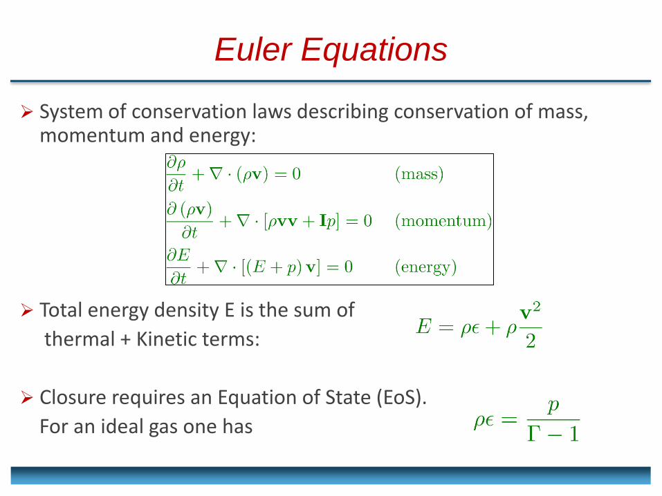
Euler Equations
System of conservation laws describing conservation of mass, momentum and energy:
Total energy density E is the sum of
thermal + Kinetic terms:
Closure requires an Equation of State (EoS).
For an ideal gas one has
Euler Equations: Characteristic Structure
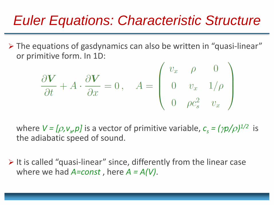
The equations of gasdynamics can also be written in “quasi-linear” or primitive form. In 1D:
where V = [,vx,p] is a vector of primitive variable, cs = (p/)1/2 is the adiabatic speed of sound.
It is called “quasi-linear” since, differently from the linear case where we had A=const , here A = A(V).
Euler Equations: Characteristic Structure
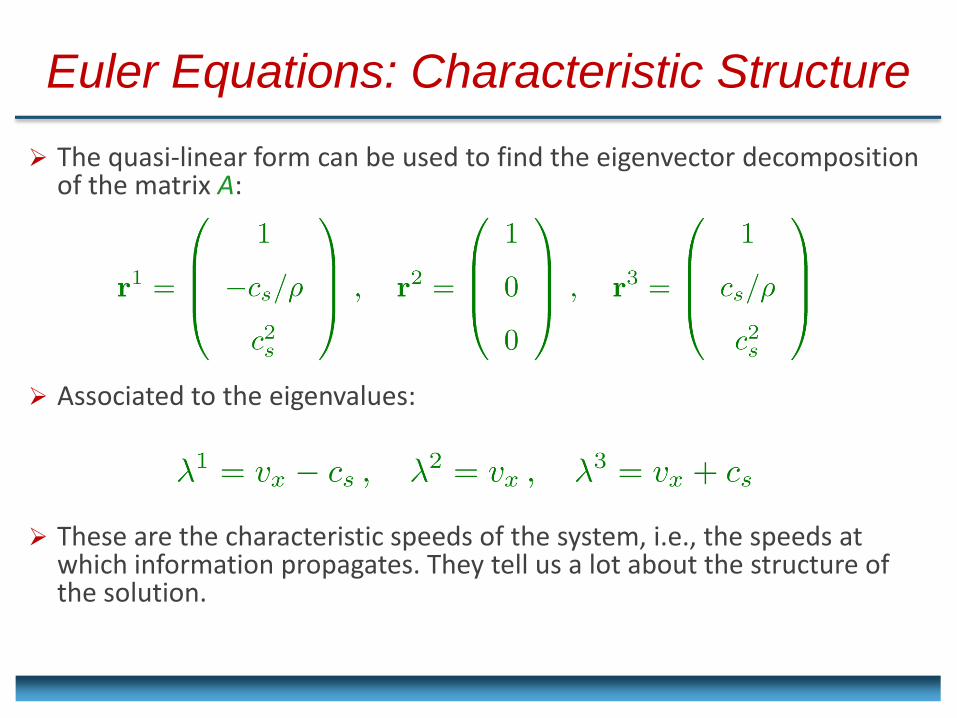
The quasi-linear form can be used to find the eigenvector decomposition of the matrix A:
Associated to the eigenvalues:
These are the characteristic speeds of the system, i.e., the speeds at which information propagates. They tell us a lot about the structure of the solution.
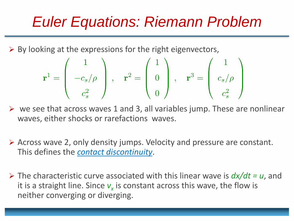
By looking at the expressions for the right eigenvectors,
we see that across waves 1 and 3, all variables jump. These are nonlinear waves, either shocks or rarefactions waves.
Across wave 2, only density jumps. Velocity and pressure are constant. This defines the contact discontinuity.
The characteristic curve associated with this linear wave is dx/dt = u, and it is a straight line. Since vx is constant across this wave, the flow is neither converging or diverging.
Euler Equations: Riemann Problem
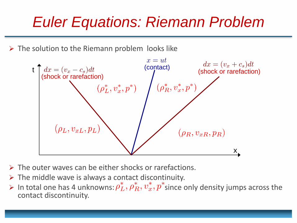
The solution to the Riemann problem looks like
The outer waves can be either shocks or rarefactions. The middle wave is always a contact discontinuity. In total one has 4 unknowns: , since only density jumps across the
contact discontinuity.
Euler Equations: Riemann Problem
x
t (contact)
(shock or rarefaction) (shock or rarefaction)
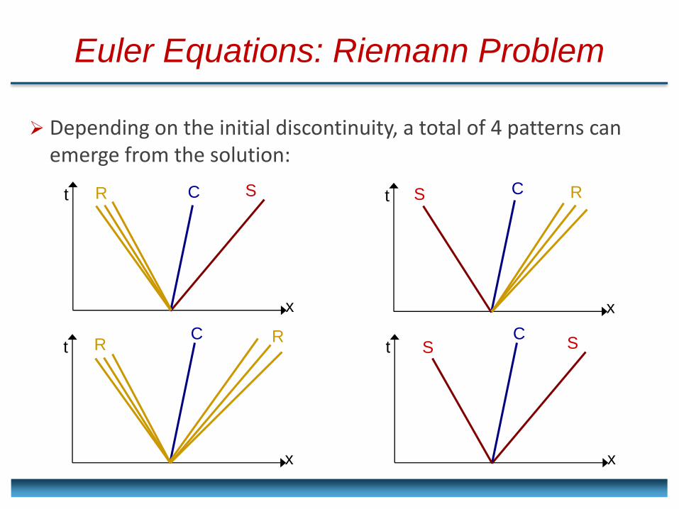
Euler Equations: Riemann Problem
Depending on the initial discontinuity, a total of 4 patterns can emerge from the solution:
x
t C S R
x
t C S R
x
t C
R
x
t C
S S R
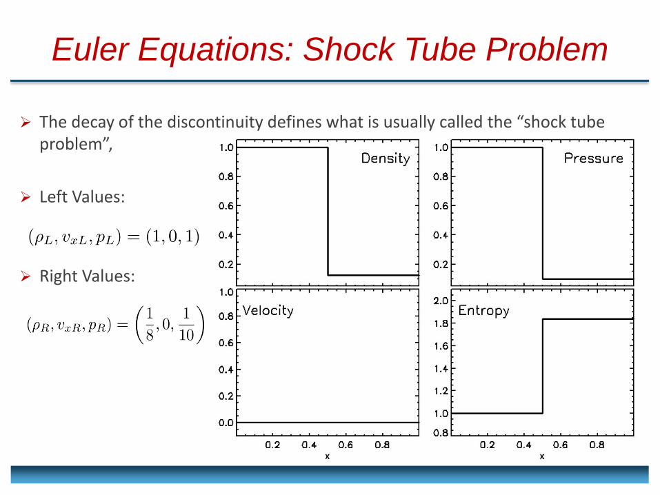
Euler Equations: Shock Tube Problem
The decay of the discontinuity defines what is usually called the “shock tube problem”,
Left Values:
Right Values:
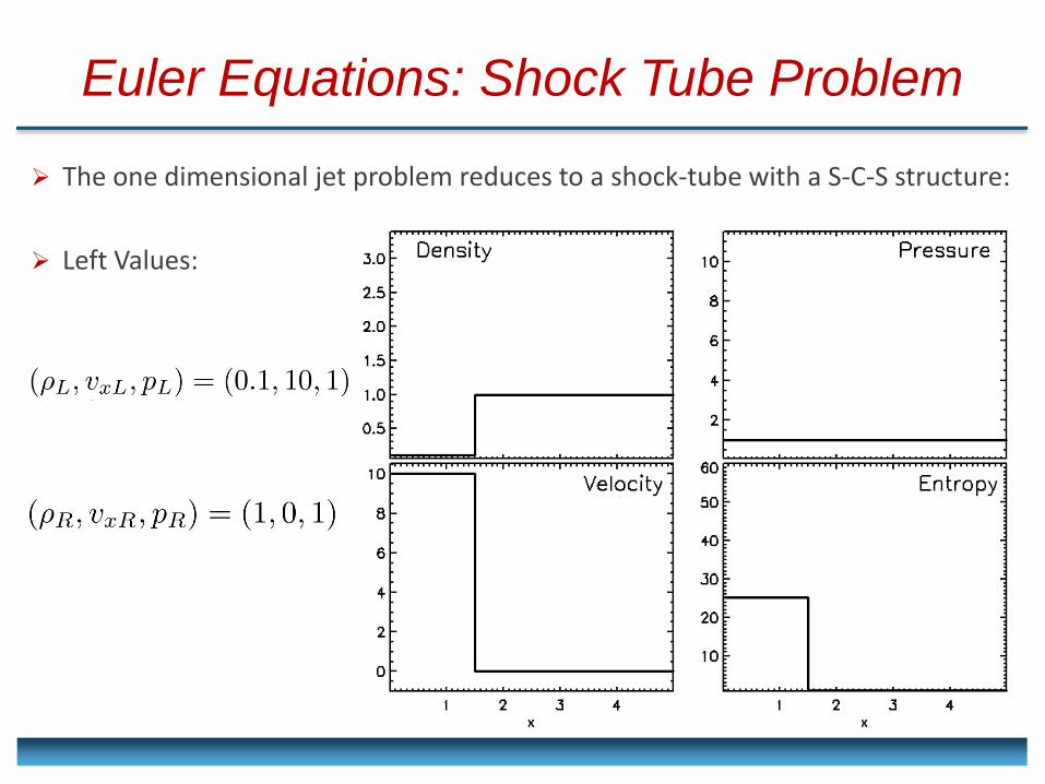
Euler Equations: Shock Tube Problem
The one dimensional jet problem reduces to a shock-tube with a S-C-S structure:
Left Values:
Right Values:
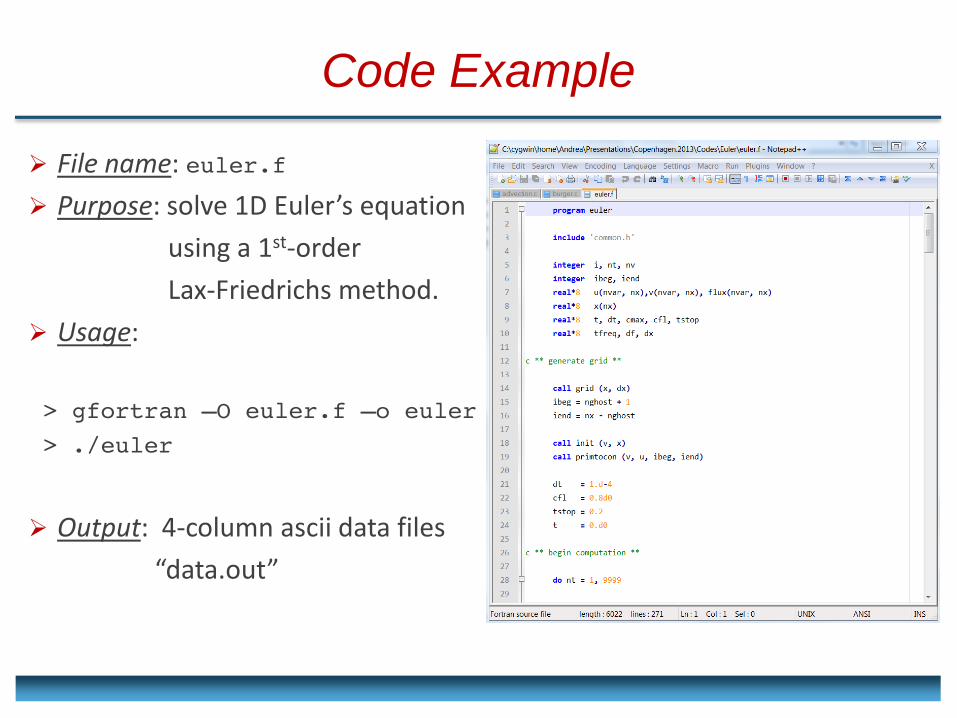
File name: euler.f
Purpose: solve 1D Euler’s equation
using a 1st-order
Lax-Friedrichs method.
Usage:
> gfortran –O euler.f –o euler
> ./euler
Output: 4-column ascii data files
“data.out”
Code Example
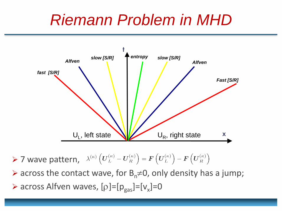
Riemann Problem in MHD
7 wave pattern,
across the contact wave, for Bn0, only density has a jump;
across Alfven waves, []=[pgas]=[vx]=0
Fast [S/R]
fast [S/R]
x
Alfven
entropy slow [S/R] Alfven
UL, left state UR, right state
t
slow [S/R]
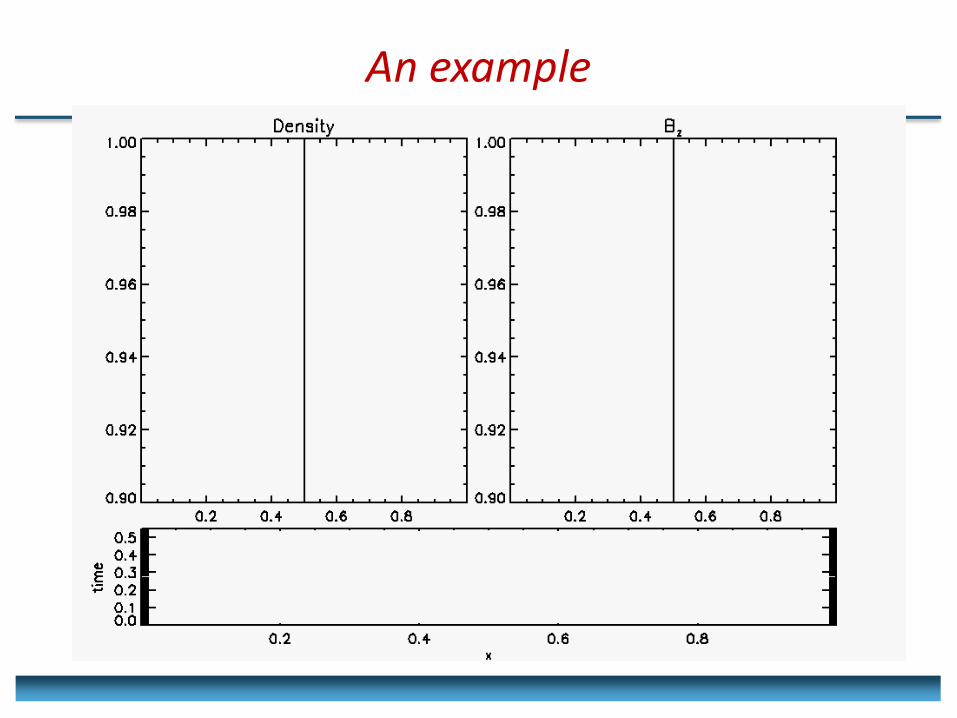
An example
Solving the Riemann Problem
The full analytical solution to the Riemann problem for the Euler equation can be found, but this is a rather complicated task (see the book by Toro).
In general, approximate methods of solution are preferred.
The advantage of using approximate solvers is the reduced computational costs and the ease of implementation.
The degree of approximation reflects on the ability to “capture” and spread discontinuities over few or more computational zones.
Solving the Riemann Problem
Exact Riemann solvers (nonlinear) Full nonlinear solution:
Expensive / impracticable for heavily usage in upwind codes;
Linearized Riemann solvers (Roe type) require characteristic decomposition in eigenvectors
may be prone to numerical pathologies
HLL-type Riemann solvers (guess-based) based on guess to the signal speeds and on the integral average of the
solution over the Riemann Fan;
fewer waves are considered in the solution;
preserve positivity;
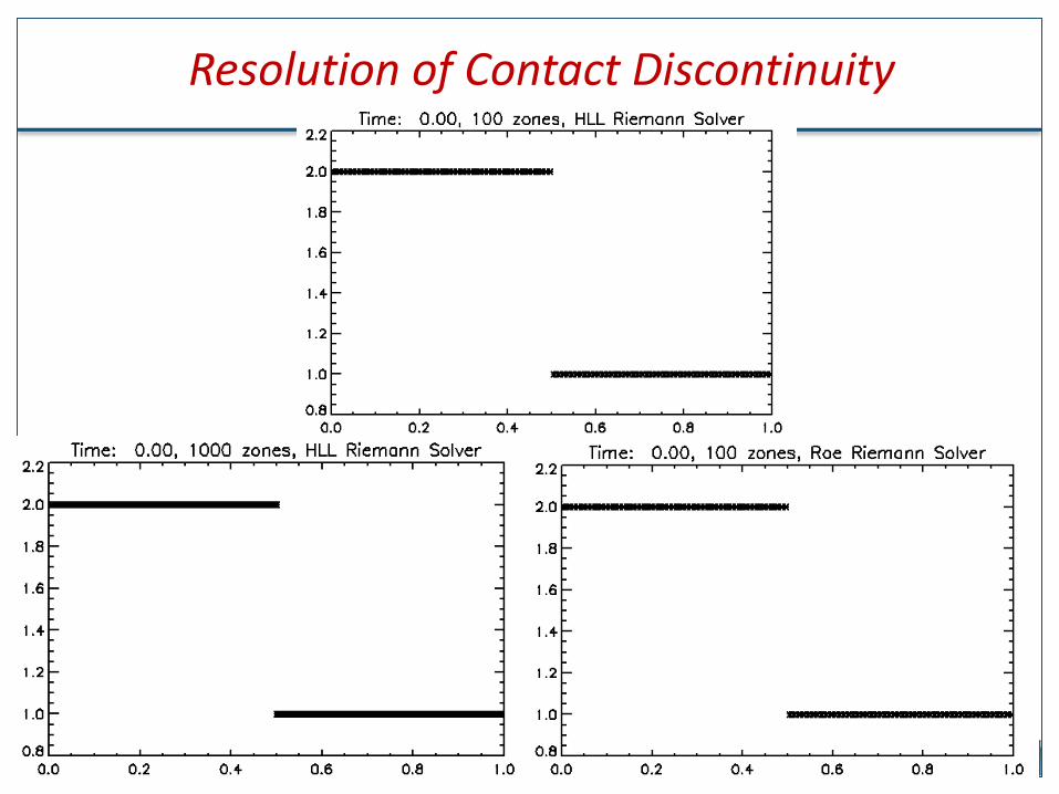
Resolution of Contact Discontinuity
HIGH-ORDER SCHEMES
2f. BASIC DISCRETIZATION METHODS FOR HYPERBOLIC PDE:
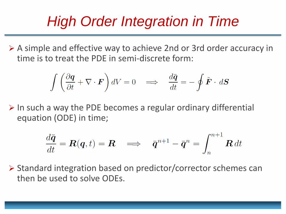
High Order Integration in Time
A simple and effective way to achieve 2nd or 3rd order accuracy in time is to treat the PDE in semi-discrete form:
In such a way the PDE becomes a regular ordinary differential equation (ODE) in time;
Standard integration based on predictor/corrector schemes can then be used to solve ODEs.
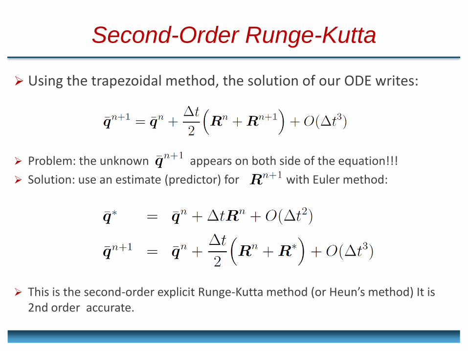
Second-Order Runge-Kutta
Using the trapezoidal method, the solution of our ODE writes:
Problem: the unknown appears on both side of the equation!!!
Solution: use an estimate (predictor) for with Euler method:
This is the second-order explicit Runge-Kutta method (or Heun’s method) It is 2nd order accurate.
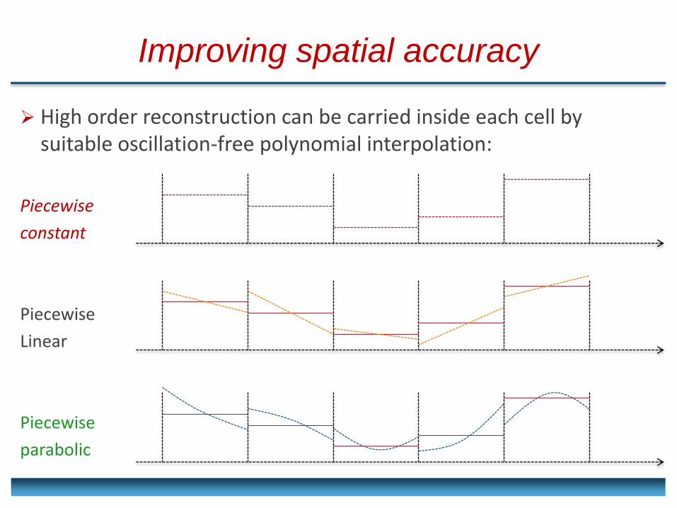
Improving spatial accuracy
High order reconstruction can be carried inside each cell by suitable oscillation-free polynomial interpolation:
Piecewise
constant
Piecewise
Linear
Piecewise
parabolic
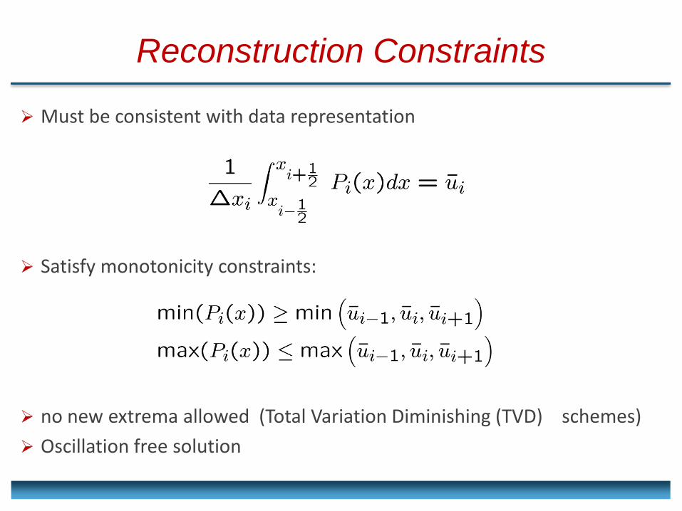
Reconstruction Constraints
Must be consistent with data representation
Satisfy monotonicity constraints:
no new extrema allowed (Total Variation Diminishing (TVD) schemes)
Oscillation free solution
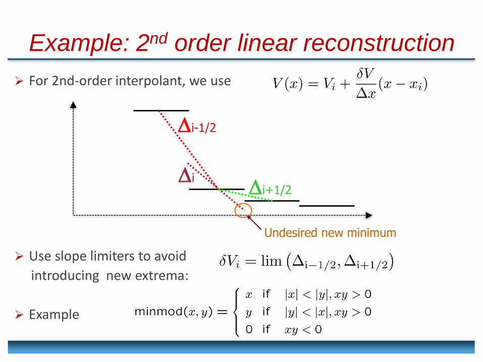
Example: 2nd order linear reconstruction
For 2nd-order interpolant, we use
Use slope limiters to avoid
introducing new extrema:
Example
i-1/2
i+1/2 i
Undesired new minimum
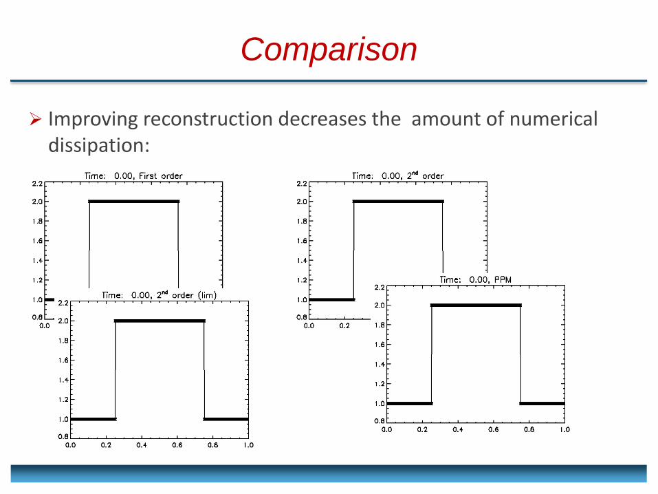
Comparison
Improving reconstruction decreases the amount of numerical dissipation:
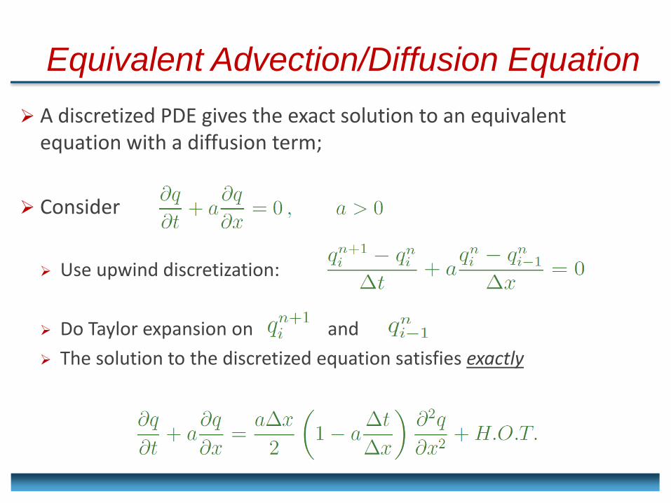
Equivalent Advection/Diffusion Equation
A discretized PDE gives the exact solution to an equivalent equation with a diffusion term;
Consider
Use upwind discretization:
Do Taylor expansion on and
The solution to the discretized equation satisfies exactly
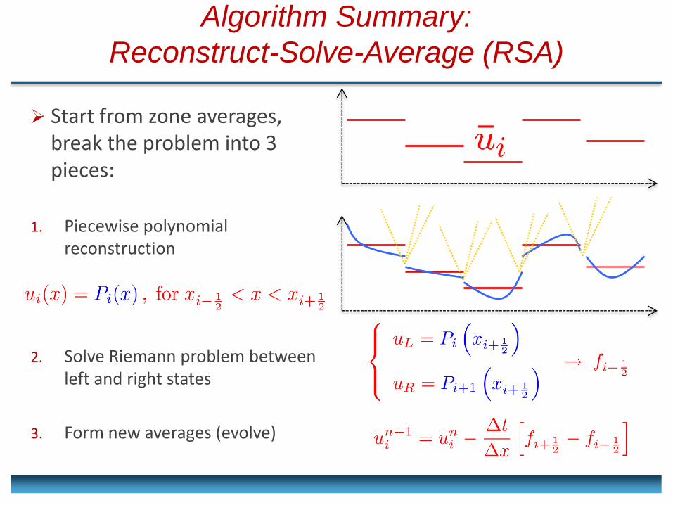
Algorithm Summary:
Reconstruct-Solve-Average (RSA)
Start from zone averages, break the problem into 3 pieces:
1. Piecewise polynomial reconstruction
2. Solve Riemann problem between left and right states
3. Form new averages (evolve)
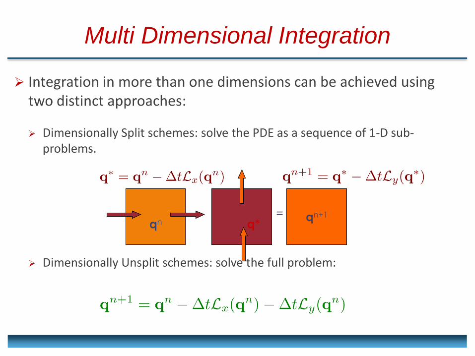
Multi Dimensional Integration
Integration in more than one dimensions can be achieved using two distinct approaches:
Dimensionally Split schemes: solve the PDE as a sequence of 1-D sub-problems.
Dimensionally Unsplit schemes: solve the full problem:
qn
q* qn+1 =
Useful Books

The End


![Geophysical & Astrophysical Fluid Dynamics...Downloaded By: [Soward, Andrew] At: 15:19 5 March 2008 Geophys. Astrophys. Fluid Dynamics, Vol. 72, pp. 107-144 Reprints available directly](https://img.pdfslide.us/doc/110x75/5f3a8fd4517cdc6d1474968c/geophysical-astrophysical-fluid-downloaded-by-soward-andrew-at-1519.jpg)


![Geophysical & Astrophysical Fluid Dynamics · Downloaded By: [University of Colorado, Boulder campus] At: 05:39 1 October 2007 Geophys. Asrrophys. Fluid Dymics.Vol. 93, pp. 221-252](https://img.pdfslide.us/doc/110x75/5f02d29a7e708231d4062f38/geophysical-astrophysical-fluid-dynamics-downloaded-by-university-of-colorado.jpg)