Geophysical & Astrophysical Fluid Dynamics Simple models ...nas13/AS/1993GAFD_Belyanin_etal_Nonlinear... · To link to this Article: DOI: 10.1080/03091929308203569 URL: ... field

PLEASE SCROLL DOWN FOR ARTICLE

This article was downloaded by:On: 6 January 2010Access details: Access Details: Free AccessPublisher Taylor & FrancisInforma Ltd Registered in England and Wales Registered Number: 1072954 Registered office: Mortimer House, 37-41 Mortimer Street, London W1T 3JH, UK

Geophysical & Astrophysical Fluid DynamicsPublication details, including instructions for authors and subscription information:http://www.informaworld.com/smpp/title~content=t713642804

Simple models of nonlinear fluctuation dynamoMikhail Belyanin a; Dmitry Sokoloff a; Anvar Shukurov b

a Physics Department, Moscow State University, Moscow, Russia b Computing Centre, Moscow StateUniversity, Moscow, Russia

To cite this Article Belyanin, Mikhail, Sokoloff, Dmitry and Shukurov, Anvar(1993) 'Simple models of nonlinearfluctuation dynamo', Geophysical & Astrophysical Fluid Dynamics, 68: 1, 237 — 261To link to this Article: DOI: 10.1080/03091929308203569URL: http://dx.doi.org/10.1080/03091929308203569

Full terms and conditions of use: http://www.informaworld.com/terms-and-conditions-of-access.pdf

This article may be used for research, teaching and private study purposes. Any substantial orsystematic reproduction, re-distribution, re-selling, loan or sub-licensing, systematic supply ordistribution in any form to anyone is expressly forbidden.

The publisher does not give any warranty express or implied or make any representation that the contentswill be complete or accurate or up to date. The accuracy of any instructions, formulae and drug dosesshould be independently verified with primary sources. The publisher shall not be liable for any loss,actions, claims, proceedings, demand or costs or damages whatsoever or howsoever caused arising directlyor indirectly in connection with or arising out of the use of this material.

http://www.informaworld.com/smpp/title~content=t713642804

http://dx.doi.org/10.1080/03091929308203569

http://www.informaworld.com/terms-and-conditions-of-access.pdf

Geophw. Asrrophys. Nuid Dynamics, Vol. 68, pp. 237-261 Reprints available directly from the publisher Photocopying permitted by license only

0 1993 Gordon and Breach Science Publishers S.A. Printed in the United States of America

SIMPLE MODELS OF NONLINEAR FLUCTUATION DYNAMO

MIKHAIL BELYANIN and DMITRY SOKOLOFF

Physics Department, Moscow State University, Moscow 119899, Russia

ANVAR SHUKUROV

Computing Centre, Moscow State University, Moscow 119899, Russia

(Received 25 July 1991; in final form 7 February 1992)

We discuss asymptotic solutions of nonlinear steady-state equations of the fluctuation dynamo, i.e. equations describing generation of a random magnetic field in a random mirror symmetric flow of conducting fluid. The flow is assumed to be locally homogeneous and isotropic and the correlation scale I is considered to be small in comparison to the size of the region occupied by the flow, L. These presumptions admit a closed nonlinear equation for the mean energy density of the magnetic field whose solutions are considered here for I/L<c 1.

If the generation efficiency drops to zero when the magnetic energy density E reaches a certain value (of the order of the kinetic energy density EJ, then the steady-state values of E are of order E, (the equipartition dynamo). Otherwise, if the generation efficiency only declines monotonically with E remaining positive, the steady-state values of E can strongly exceed E, [by the factor (L/r)2ip with certain constant p of order unity] (the supra-equipartition dynamo). These general properties of the steady state are illustrated by two simple models of nonlinearity.

KEY WORDS: Fluctuation dynamo, nonlinear regimes, asymptotic solutions.

1. INTRODUCTION

Chaotic, mirror-symmetric motions of conducting fluid can amplify and maintain chaotic magnetic fields provided the magnetic Reynolds number is sufficiently large, R,S102 [see the review of Zeldovich et al. (1988) and references therein]. This mechanism of generation of chaotic magnetic fields can be encountered in any object where conducting fluid resides in a turbulent state-in intergalactic gas of galaxy clusters (Ruzmaikin et al., 1989), interstellar gas of spiral and elliptic galaxies (De Young, 1980; Sokoloff et al., 1990), interplanetary plasma (Ruzmaikin et al., 1992) and some industrial devices (Kirko, 1985). The generated chaotic magnetic field can be quantitatively characterized by the correlation tensor ( H i t , x) H i t , y)) = &‘ijt, x, y) where (*..) denotes the ensemble averaging. When the random motions are locally homogeneous and isotropic and, in addition, their correlation scale 1 is much smaller than the region size L, the approximation of local homogeneity and isotropy applies also to the random magnetic field Hi( t , x). In this case the correlation tensor Xi,(t, x, y)

231

Downloaded At: 17:17 6 January 2010

238 MIKHAIL BELYANIN, DMITRY SOKOLOFF AND ANVAR SHUKUROV

can be represented as

where r=$x+y), E is the mean energy density of magnetic field and H , is the homogeneous, isotropic correlation tensor. In the framework of this approximation, solution of the problem of evolution of the tensor 3Pijt, x, y) naturally splits into two stages. For &=(I,’L)’+O, at the zeroth approximation one solves the problem of evolution of the local tensor H i p To this approximation, E = const x exp(y,t). Equation for the leading term in the expansion of H i j in powers of c1I2 has been derived by Kazantsev (1967) and Kraichnan and Nagarajan (1967); this equation has been a subject of thorough studies reviewed by Zeldovich et al. (1988, 1990).

To the next approximation in E, when the dependence of the flow scale and velocity on position is taken into account, the local “growth rate” of magnetic energy, yo, becomes a function of r and the mean energy density E is governed by the following equation which has been derived by Maslova et al. (1987) for the case of the vanishing mean velocity:

i?E -=;to(r) E + E A E . at

Equation (1) is given in a dimensionless form with the scales measured in units of L, time normalized by l / u ( u is the characteristic turbulent velocity) and E = ( I / L ) ~ is the dimensionless turbulent diffusivity. The coefficient E is much smaller than unity as long as 1 << L. In galaxy clusters, galactic coronae and the solar wind, E is as low as lo-’.

After a certain period, magnetic energy becomes comparable to the kinetic energy and magnetic field affects the velocity field significantly. It is natural to expect that the result is a dynamic equilibrium in which the mean magnetic energy is stationary. Generally, in order to study the steady state one should consider also the Navier-Stokes equation which includes the magnetic force. The complexity of the resulting problem is enormous. However, one can invoke simple models of nonlinearity, e.g. consider the local growth rate y as a monotonically decreasing function of the mean energy density E. In fact, this approach is frequently used in nonlinear mean-field dynamo models. As far as dE/d t=O in equation (l), we have the following equation for the steady state:

y(E, r) E + E AE = 0. (2)

This phenomenological introduction of nonlinearity into the dynamo equations is far from being universal. At the present level of understanding, it seems also plausible that nonlinear effects result in time dependence of the tensor Hi,(x-y1), i.e. the nonlinear effects can be of a local nature. From the formal viewpoint, this means that the Kazantsev equation becomes nonlinear. Coefficients in the Kazantsev equation are determined by the correlaton tensor of the velocity field and this approach


NONLINEAR FLUCTUATION DYNAMO 239

implies that saturation of the field growth is associated with a significant modification of such flow parameters as, say, the correlation scale or time.

Alternatively, the magnetic field influence on the flow can possibly be described phenomenologically in terms of magnetic energy sinks whose intensity grows with E. In this case the steady state can be described by (2).

Both approaches deserve careful analysis. It seems quite possible that both scenarios can be realized in different physical situations. This paper is devoted to analysis of the latter possibility which seems to us more plausible from the physical viewpoint. Indeed, direct estimates of the magnetic Reynolds number for undoubtedly nonlinear dynamo systems (e.g., the Sun, interstellar and intergalactic medium), based on the observed values of the turbulent velocity field, yield values far exceeding the critical value, 1: lo2 (cf. Ruzmaikin et al., 1989; Sokoloff et al., 1990). This implies that the growing magnetic fields affect the magnetic dissipation mechanism and/or the transfer of magnetic energy into the kinetic one and vice versa, rather than the characteristic scale and velocity of motions.

As shown by Dittrich et al. (1988) for an individual realization of the random magnetic field generated by the dynamo, the intermittent distribution of the magnetic field typical of the kinematic fluctuation dynamo is preserved in the steady state, i.e. the tensor H,,{lx-yl) does not suffer drastic modifications. We consider this fact as indirect evidence in favour of the approach chosen here.

Note that y(r) in equation (1) is real (see, e.g., Zeldovich et al., 1988). There are reasons to expect that in this case the steady-state solutions for the mean energy density E cannot be oscillatory (S. A. Kashchenko, private communication). Thus, the nonlinear problem reduces to equation (2) supplemented with appropriate boundary conditions. Below we search for its asymptotic solutions for E+O.

The existence of a formal asymptotic expansion does not guarantee the existence of the corresponding exact solution. Therefore, in Appendices A and B we prove rigorously the existence and uniqueness of solutions to (2) which have the required properties. As often happens, the proof of existence of a unique solution is much more complicated than assessment of essential features of the asymptotic solution. We have attempted to concentrate all formal arguments in the appendices while leaving the main text for the results which seem to be important for applications.

2. MODELS OF NONLINEAR DYNAMO

We consider two simple forms of nonlinearity whose analogs are well known in the mean-field dynamo theory (see Krause and Radler, 1980 and Kvasz et al., 1992 for motivation of this choice):



where yo@) is the local growth rate which follows from the kinematic dynamo problem, p is a certain constant and g can be a function of position. For the sake of definiteness, consider a spherically symmetric body and assume that chaotic motions decay at infinity which implies that the dynamo generation ceases at a certain spherical radius ro so that yo(r)>O for O<r<ro and yo(r)=O for r 2 r o , where r = Irl and ro=O(l). By the order of magnitude, we have yo(r)=O(u/l) in dimensional units (Zeldovich et al., 1988).

We also presume that yb(ro) < 0 (here and below the prime denotes derivative with respect to r). The condition $,(ro)#O has a rather general character. Indeed, at the radius r = ro the magnetic Reynolds number decreases down to a certain critical value Rmcr= lo2, so that yo 3 0 for R m 3 R,,,. As far as aYO/aRm(R,=R,,,>O and R , is a monotonically decreasing function of r, we obtain the inequality yb(ro) to. A typical form of the function yo(') is shown in Figure 1.

We consider two particular forms of nonlinearity, (3)-and (4), expecting that the resulting solutions will reflect generic properties of the nonlinear dynamo. For the nonlinearity of the form (3) y, as a function of E, has a positive root. For this ultimate reason, this form of nonlinearity corresponds to the steady state with E(r) of order unity in E. In contrast, the function y(E,r) of the form (4) is always positive and, therefore, E can acquire large values (of the order of E - ''''-see Section 4 and Appendix B). We believe that these two particular cases, (3) and (4), together provide an adequate description of generic properties of a steady nonlinear dynamo. As a matter of fact, the basic properties of solutions discussed below are determined only by the aforementioned general properties of the chosen nonlinearities. The magnitude of the nonlinear solution is of order unity when the function y(E) has a positive root and E >> 1 if y(E) never vanishes.

Figure 1 Reynolds number decreases down to the critical value and yo(r)=O for r>r,,.

Typical forms of the functions y,,(r) (solid) and g(r) (dashed). At the radius ro the magnetic


NONLINEAR FLUCTUATION DYNAMO 24 1

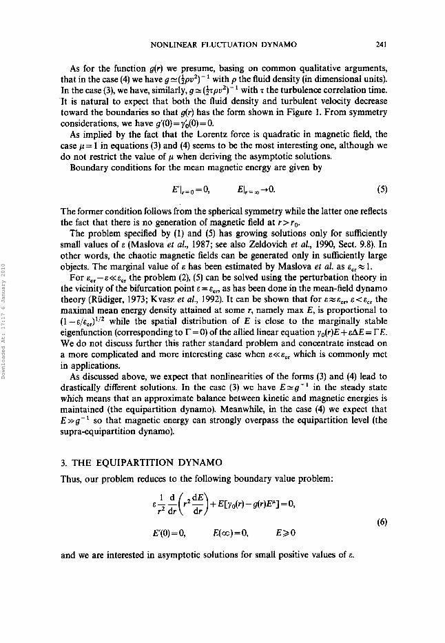
As for the function g(r ) we presume, basing on common qualitative arguments, that in the case (4) we have g=( ipu2) - ' with p the fluid density (in dimensional units). In the case (3), we have, similarly, g N (&pu2)- with z the turbulence correlation time. 'It is natural to expect that both the fluid density and turbulent velocity decrease toward the boundaries so that g(r) has the form shown in Figure 1. From symmetry considerations, we have g'(0) = yb(0) = 0.

As implied by the fact that the Lorentz force is quadratic in magnetic field, the case p= 1 in equations (3) and (4) seems to be the most interesting one, although we do not restrict the value of p when deriving the asymptotic solutions.

Boundary conditions for the mean magnetic energy are given by

The former condition follows from the spherical symmetry while the latter one reflects the fact that there is no generation of magnetic field at r>ro .

The problem specified by (1) and (5) has growing solutions only for sufficiently small values of E (Maslova et al., 1987; see also Zeldovich et al., 1990, Sect. 9.8). In other words, the chaotic magnetic fields can be generated only in sufficiently large objects. The marginal value of E has been estimated by Maslova et al. as E,,X 1.

For E,,-E<<E,, the problem (2), ( 5 ) can be solved using the perturbation theory in the vicinity of the bifurcation point E =E,,, as has been done in the mean-field dynamo theory (Rudiger, 1973; Kvasz et al., 1992). It can be shown that for EXE, , , E < E , , the maximal mean energy density attained at some r, namely max E, is proportional to (1 - E / E , , ) ' / ~ while the spatial distribution of E is close to the marginally stable eigenfunction (corresponding to = 0) of the allied linear equation y,(r)E + EAE = TE. We do not discuss further this rather standard problem and concentrate instead on a more complicated and more interesting case when E<<E,, which is commonly met in applications.

As discussed above, we expect that nonlinearities of the forms (3) and (4) lead to drastically different solutions. In the case (3) we have E = g - ' in the steady state which means that an approximate balance between kinetic and magnetic energies is maintained (the equipartition dynamo). Meanwhile, in the case (4) we expect that E>>g-' so that magnetic energy can strongly overpass the equipartition level (the supra-equipartition dynamo).

3. THE EQUIPARTITION DYNAMO

Thus, our problem reduces to the following boundary value problem:

+ E[yo(r) - g(r)E'] =0, r2 dr

E(0) = 0, E( 00) = 0, E > O

and we are interested in asymptotic solutions for small positive values of E .


242 MIKHAIL BELYANIN, DMITRY SOKOLOFF A N D ANVAR SHUKUROV

We presume that the solution has the scale of order unity in the major portion of the considered volume, i.e. E‘/E = O( 1). This solution, called the regular one, can be represented as a power series in E :

50

E = C P E E , . n = O

This series should be substituted into (6) and the terms with equal powers of E should be combined. As a result, the first two terms in the expansion are given by

for r <r*, for r > r*,

and

for r > r * .

(7)

In (7) and (8) we introduce the radius r* whose nature can be clarified as follows. The function Eo(r) satisfies equations (6) to the accuracy of O(E) everywhere except at the point r=r* at which occurs a discontinuity, either of the function E , itself (when r* # ro) or of its derivative (when r* = ro). We can also show that r* < ro. Indeed, the term &El exceeds in absolute value E , at r = ro because yo(r,) = 0. This indicates, in particular, that the solution given by (7) and (8) becomes inapplicable when r approaches ro, so that r* c r , . As shown in Appendix A, ro -r* = O ( E ” ~ ) provided d2[(yo/g)””]/dr2 < 0 for 0 < r < r,. Otherwise, the value of ro -r* can be different but remains small. A general form of the solution is shown in Figure 2. In the case considered here, when yb(0) = g‘(0) = 0, the obtained leading-order solution automatically satisfies the boundary condition E‘(0) = 0.

The regular solution, whose two leading terms are given by (7) and (8), is inapplicable at r>r* where we have IE‘/E(>>l. In common situations, an extreme inequality of this kind occurs due to the presence of a boundary layer within which the solution changes rapidly so that (E’I >> 1 and E = O( 1). In our case, however, we have E’ = O( 1) and E = O ( E ” ~ ) for r = r* and the exact solution does not contain classical boundary layers. The exact solution is discussed in detail in Appendix A where, in particular, we prove its existence and uniqueness. From the viewpoint of applications, it is essential that the exact solution decreases monotonically with the radius and has the order of magnitude &/r3 for r>>ro (for p = 1) while expressions (7) and (8) can be used for r < r*. The solution discussed above is such that y(E, r ) 20 for r < r* and y(E, r ) < O for r>r* . One can also consider a slightly different form of nonlinearity, y(E, r) = yo(‘)[ 1 -g(r )Ep] . In this case the solution for r < r* is physically similar to that discussed above, with Eo=g-‘ / ’ for r<r* . However, both the value of r* and the behaviour of E at r+oo are different from the results obtained for the form (3).



, I I I I

r* ro r Figure 2 A schematic representation of the unique solution of the boundary value problem (6). Solid line: the exact solution E(r). Dashed line: the zeroth approximation E,(r) to the regular solution.

We should note that a general singular perturbation theory discussed in detail by, e.g., Vasilyeva and Butuzov (1973)“’, does not work in our case. In Appendix A we propose the theory which is applicable to equation (1) with nonlinearity of the form (3).

Behaviour of the solution for r>r* is somewhat sensitive to details of the form of the functions yo(‘) and g(r). For instance, the results given above are valid when g(r) tends to infinity for r+oo not slower than a power-law function but not faster than an exponential function.

4. THE SUPRA-EQUIPARTITION DYNAMO

In this section we consider the following boundary value problem:

(9) E(0) = 0, E( CO) = 0, E>O.

In Appendix B we also discuss the case of nonlinearity with arbitrary power p (> 1) (for p c 1 the nonlinearity is probably too weak to ensure the development of a steady state).

In contrast to the problem (6), this problem is a regularly perturbed one. This is implied by the fact that the second term on the left-hand side of equation (9) does

( l ) Unfortunately, this monograph has not been translated into Western languages. For the Western reader, we can also refer to Tikhonov et al. (1985) and Smith (1985).



not vanish identically for any non-vanishing E, so that the term with the derivative cannot be neglected at any position. A rigorous proof of the uniqueness of this solution can be found in Appendix B. In order to derive an asymptotic solution of the problem (9), it is important to realize that the solution tends to infinity for E+O.

Consider first equation (9) for r > ro where yo =O. Obviously, we have

where the constant C, will be determined below (see Section 5 for discussion of this behaviour with the radius).

Since we have a regularly perturbed problem, the solution can be expanded in the series of the form

30

E = E - ' 1 E"E, n = O

(see Appendix B for a formal proof of this fact). For the leading-order term we have the following boundary value problem:

Eb(0) = 0,

whose solution is given by

where 0 < r c ro and C, is an arbitrary constant which will be determined below.

conditions : Solutions (10) and (1 1) should be matched at r = ro by imposing the following two

E(ro - 0) = E(ro + 0), E'(ro - 0) = E'(ro + 0).

We match both the solution and its derivative because the considered differential equation (1) is of the second order. These conditions allow us to determine two constants"', C , and C2. After some algebra, the result reduces to

for r > ro.

12) More precisely, here we obtain the leading term in the expansion C , = & - I ZE"~',"', the higher terms can be obtained from matching the form (10) with a higher-order solution of equation (9) for r<rW



The next higher term in the expansion of the solution in powers of E has the order of magnitude O(1) (see Appendix B).

5. DISCUSSION

The asymptotic solutions derived above decay at infinity unusually slowly. The behaviour at infinity which is usual in dynamo theory, H a r - j for r+m, would correspond to E a r - 6 . Meanwhile, we obtain E a r p 3 for the nonlinearity of the form (3) and E a r - ' for the nonlinearity (4) for 1-00 and p= 1. We should emphasize that these results refer to f i =const, where f i is the dimensional magnetic diffusivity. Meanwhile, the law E a r F 6 corresponds to a conducting dynamo volume surrounded by vacuum, i.e. p+m for r - a . Thus, the usual behaviour at infinity is due to inhomogeneity of /I.

Our results can be easily generalized to the case of arbitrary continuous dependence of B on r. For example, in the case of a smooth dependence, equation (2) takes the form

y ( E , r ) E + & L r2 d(r2/3(r)$)=0. dr

The transformation of the independent variable r a x chosen in such way that

reduces this equation to the form (2) in terms of the independent variable x and with y replaced by r4(x)x -4fly.

When B(r) monotonically increases with r for r>>1, we arrive at the following inequality :

x - ' < f i - ' { : ~-~du=[rfi(r)]- ' .

Thus, E decays at infinity more rapidly than [r/l(r)]-' for both types of nonlinearity and the vacuum behaviour E a r - 6 corresponds to the growth ofg with r at least as r5.

In the case when f i tends to infinity at a finite radius r=rm, the presumption of local homogeneity and isotropy is violated near the boundary and, strictly speaking, equation (2) is inapplicable. However, meaningful solutions for r < rm can be obtained after introduction of the boundary condition E(rm) = 0.

We have discussed a spherically symmetric case. The leading-order solutions can be also obtained without the presumption of spherical symmetry. However, rigorous justification of the asymptotic solutions similar to that presented in Appendices A and B is much more complicated in absence of spherical symmetry.

As we have seen above, the form and the magnitude of the steady solution crucially depend on the particular functional form of the nonlinearity. In Figure 3 we plot E , for both types of nonlinearity. [In particular, solution (12) decays at infinity at a considerably smaller rate than the solution described in Section 3.1 This implies that



I \ \

1

T O r Figure 3 An illustration of the difference between asymptotic solutions for the two types of nonlinearity (3) (dashed) and (4) (solid). The solid line shows the leading-order solution (12) for the supra-equipartition dynamo, E,(O)= O(E- ’). The dashed line shows the leading-order solution (7) for the equipartition dynamo, Eo(0)=O(l); this solution becomes inapplicable for r > r * as indicated by the dotted line.

comparison of solutions derived here with observations of steady distributions of magnetic energy can allow us to choose the most adequate mechanism of nonlinear saturation of the dynamo. For instance, the nonlinearity (4) seems to be more suitable in modelling the dynamo in galaxy clusters (cf. Ruzmaikin et al., 1989).

We should note one more important difference between solutions with the two forms of nonlinearity considered here. In the case (4) the magnetic energy density exceeds the kinetic energy density by the factor E-”” . We call this regime the supra-equipartition dynamo. One usually presumes that fluid motions are able to amplify magnetic field only up to the level of equipartition with kinetic energy. However, we emphasize that this restriction is removed and magnetic energy can exceed the equipartition level provided the magnetic field is close to a force-free configuration. On the one hand, theory of fluctuation dynamo indicates that the generated magnetic ropes have helical shape and, therefore, the magnetic field approaches a force-free configuration (Zeldovich et al., 1988, 1990). On the other hand, observations of the galaxy cluster Cygnus A, where the fluctuation dynamo can be operative, directly reveal concentrated magnetic fields whose strength significantly exceeds the equipartition level (Dreher et al., 1987).

Acknowledgements The authors are grateful to N. N. Nefedov who attracted our attention to advantages of the differential inequalities technique. We thank V. F. Butuzov for his generous attention to our work. It is a pleasure to acknowledge the careful reading and useful comments of an anonymous referee, which improved the presentation. DS is grateful to Lunokhod Ltd for financial support.



References Chang, K. W. and Howes, F. A., Nonlinear Singular Perturbation Phenomena (Theory and Applications),

De. Young, D. S., “Turbulent generation of magnetic fields in extragalactic radio sources,” Astrophys. J.

Dittrich, P., Molchanov, S. A., Ruzmaikin, A. A. and Sokoloff, D. D., “Stationary distribution of the value

Dreher, J. W., Carilli, C. L. and Perley, A., “The Faraday rotation of Cygnus A: magnetic fields in cluster

Hartman, P., Ordinary Differential Equations. Baltimore (1973). Kazantsev, A. P., “Enhancement of a magnetic field by a conducting fluid,” Sou. Phys. JETP 26,1031 -1039

Kirko, G. E., Generation and Self-Excitation of Magnetic Fields in Technical Devices, Nauka, Moscow (in

Kraichnan, R. H. and Nagarajan, S., “Growth of turbulent magnetic fields,” Phys. Fluids 10,859-870( 1967). Krause, F. and Radler, K.-H., Mean-Field Magnetohydrodynamics and Dynamo Theory, Pergamon Press,

Oxford (1980). Kvasz, L., Sokoloff, D. and Shukurov, A., “A steady state of the disk dynamo,” Geophys. Astrophys. Fluid

Dynam. 65,23 1-244 (1992). Maslova, T. B., Shumkina, T. S., Ruzmaikin, A. A. and Sokoloff, D. D., “Selfexcitation of fluctuating

magnetic fields in a spatially bounded random flow,” Dokl. Akad. Nauk SSSR 294,1373- 1376 (1987). Rudiger, G., “Behandlung eines enfaches hydrodynamischen Dynamos mittels Linearisierung,” Astron.

Nachr. 294, 183-186 (1973). Ruzmaikin, A., Sokoloff, D. and Shukurov, A., “The dynamo origin of magnetic fields in galaxy clusters,”

Mon. Not. R. asfr. Soc. 241, 1-14(1989). Ruzmaikin, A. A,, Sokoloff, D. D. and Shukurov, A., “Magnetic ropes in the solar wind,” J. Geophys. Res.

(in press) (1991). Smith, D. R., Singular-Perturbation Theory. An Introduction with Applications, Cambridge Univ. Press,

Cambridge (1985). Sokoloff, D., Ruzmaikin, A. and Shukurov, A., “Intermittent magnetic fields in galaxy clusters and

interstellar gas,” In: Intersiellar and Intergalactic Magnetic Fields, Proc. IA U Symp. 140, (Eds. R. Beck, P. P. Kronberg and R. Wielebinski), Kluwer Acad. Publ., Dordrecht, pp. 499-502 (1990).

Tiknonov, A. N., Vasilyeva, A. B. and Sveshnikov, A. G., Differential Equations, Springer-Verlag, Berlin (1 985).

Vasilyeva, A. B. and Butuzov, V. F., Asymptotic Expansions for Singularly Perturbed Equations, Nauka, Moscow (in Russian) (1973).

Zeldovich, Y. B., Molchanov, S. A., Ruzmaikin, A. A. and Sokoloff, D. D., “Intermittency, diffusion and generation,” Sov. Sci. Rev. C7, 2-110 (1988).

Zeldovich, Ya. B., Ruzmaikin, A. A. and Sokoloff, D. D., The Almighty Chance, World. Sci. Publ., Singapore (1990).

Springer-Verlag, Berlin (1984).

241, 81-97 (1980).

of the magnetic field in a random flow,” Magnetohydrodynamics, 24, N3,274-276 (1988).

gas,” Astrophys. J. 316, 61 1-625 (1987).

(1967).

Russian) (1985).

APPENDIX A

In this Appendix we consider the following boundary value problem:

(A. 1) E(0) = 0, E(co)=O, E 2 0 ,

where p > 1. Below we prove the existence and uniqueness of solution of problem (A.1).


248 MIKHAIL BELY ANIN, DMITRY SOKOLOFF A N D ANVAR SHUKUROV

Furthermore, we discuss in detail a nontrivial problem of matching two parts of the regular solution, (7) and (8). A similar problem arises in fluid mechanics where two parts of a regular solution match with the help of a boundary layer, i.e. there exists a region where the solution rapidly varies in space which compensates the discontinuity of the regular solution. Here we should compensate a discontinuity of the derivative of the solution. In our particular case the total solution cannot be presented as a combination of the regular one and a boundary layer (at least we have failed in attempts to do this) and we are forced to develop a specialized technique to match the two parts of the regular solution (7). Solution of this problem, which is rather complicated, is required for estimation of the order, in E, of the solution for r- co and for verification that the obtained asymptotic solution smoothly decays for r > ro.

Introduce the variable

w = Er.

In terms of this variable, the problem (A.l) reduces to

where f ( w , r ) = w(yo-gr-”w”). Before turning to the proof of existence and uniqueness of solution of problem

(A.2), we present a short review of the structure of this Appendix. First in Section A.l we prove that the exact solution has the form shown by a

solid line in Figure 2, i.e. for 0 < r < r* the curve corresponding to w lies below the curve F(r)= [r”yO(r)g-’(r)]’‘”, which corresponds to the regular solution (7), while for r > r* the solution runs above this curve.

Consider the physical meaning of our arguments. There exist two physically distinct regions, that in which magnetic field generation dominates, r Zro , and that in which magnetic diffusion prevails, r 5 ro. The parts of the solution, which can be obtained for these two regions separately (the regular solutions), cannot be matched smoothly at r=ro . Such matching is possible only at the point r* such that r o - r * = O ( l ) . As the analysis of the exact solution performed in this Appendix demonstrates, the result of such matching cannot be an asymptotic form of the exact solution. Our arguments prove that the exact solution inevitably contains a transition region r*<r<ro in which the solution transforms from the generation-type one to the diffusion-type one. It is important for applications that ro-r*<< 1, so that the regular solution, which can be evaluated without much effort, is applicable in the major portion of the region O<r<ro .

The properties of the solution are considered consequently for the ranges 0 -= r < q, q < r < ro and r > ro in Subsections A.2, A.3 and A.4, respectively. At each interval we consider the families of functions wl(r , q), wz(r, q) and w3(r, O), respectively, which parametrically depend on certain constants q and 8 and coincide with the exact



solution for some values of q and 8. In Subsection AS we match these three parts of the solution and prove that there exist unique values of q = r* and 8 which admit the required matching. At this point we determine how the solution behaves at r+ 00

and obtain the estimate I* = ro- O(E’’~). Our analysis of asymptotic solutions relies on the technique of differential

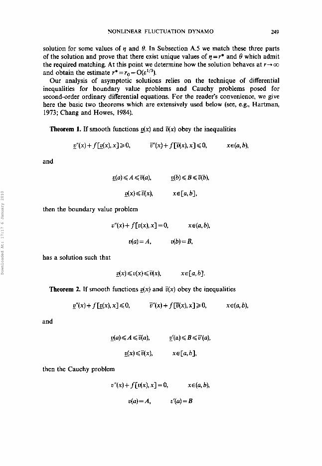
inequalities for boundary value problems and Cauchy problems posed for second-order ordinary differential equations. For the reader’s convenience, we give here the basic two theorems which are extensively used below (see, e.g., Hartman, 1973; Chang and Howes, 1984).

Theorem 1. If smooth functions d x ) and Z(x) obey the inequalities

and

then the boundary value problem

has a solution such that

Theorem 2. If smooth functions ~ ( x ) and q x ) obey the inequalities

and

then the Cauchy problem

v”(x) + f [u (x ) , x ] = 0, x E (a, b),

U(U) = A, v’(a) = B


250 MIKHAIL BELYANIN. DMITRY SOKOLOFF A N D ANVAR SHUKUROV

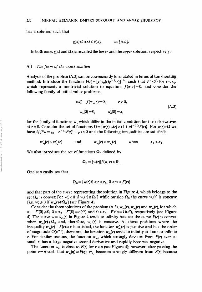
has a solution such that

In both cases ~ ( x ) and qx) are called the lower and the upper solution, respectively.

A.l The form of the exact solution

Analysis of the problem (A.2) can be conveniently formulated in terms of the shooting method. Introduce the function F(r) = [rNyo(r)g- l(r)]l'r, such that F < 0 for r < r,, which represents a nontrivial solution to equation f(w, r)=O, and consider the following family of initial value problems:

EWI: + f ( w,, r) = 0, r>O,

WAO) = 0, wh(0) = a,

for the family of functions w, which differ in the initial condition for their derivatives at r = 0. Consider the set of functions R = { w(r)lw(r) > ( 1 + p)- "NF(r)}. For w(r)~R we have d f / d w = y o - r-'wNg( 1 + p ) < 0 and the following inequalities are satisfied:

We also introduce the set of functions R, defined by

One can easily see that

R, = { w(r)(O < r < r,, 0 < w < F(r)}

and that part of the curve representing the solution in Figure 4, which belongs to the set R, is convex [or w;<O if w,(r)ER,] while outside Q, the curve w,(r) is concave [i.e. w: >, 0 if w,(r) 4 R,] (see Figure 4).

Consider the three solutions of the problem (A.3), wJr), wJr) and wa3(r), for which a1 - F'(O)2 0, 0 > ct2 - F'(0) = o(co) and O > a3 - F'(0) = 0 ( c o ) , respectively (see Figure 4). The curve w = wal(r) in Figure 4 tends to infinity because the curve F(r) is convex when waI(r)$Ro and, therefore, wJr) is concave. At those positions where the inequality w,,(r)- F ( r ) s c is satisfied, the function w:,(r) is positive and has the order of magnitude O(E- '); therefore, the function w,,(r) tends to infinity at finite or infinite r. For similar reasons, the function w,,, which strongly deviates from F(r) even at small r, has a large negative second derivative and rapidly becomes negative.

The function wa2 is close to F(r) for r < q (see Figure 4); however, after passing the point r = q such that w&) = F(q), w,, becomes strongly different from F(r) because


NONLINEAR FLUCTUATION DYNAMO 25 1

r* r, r W \

a3

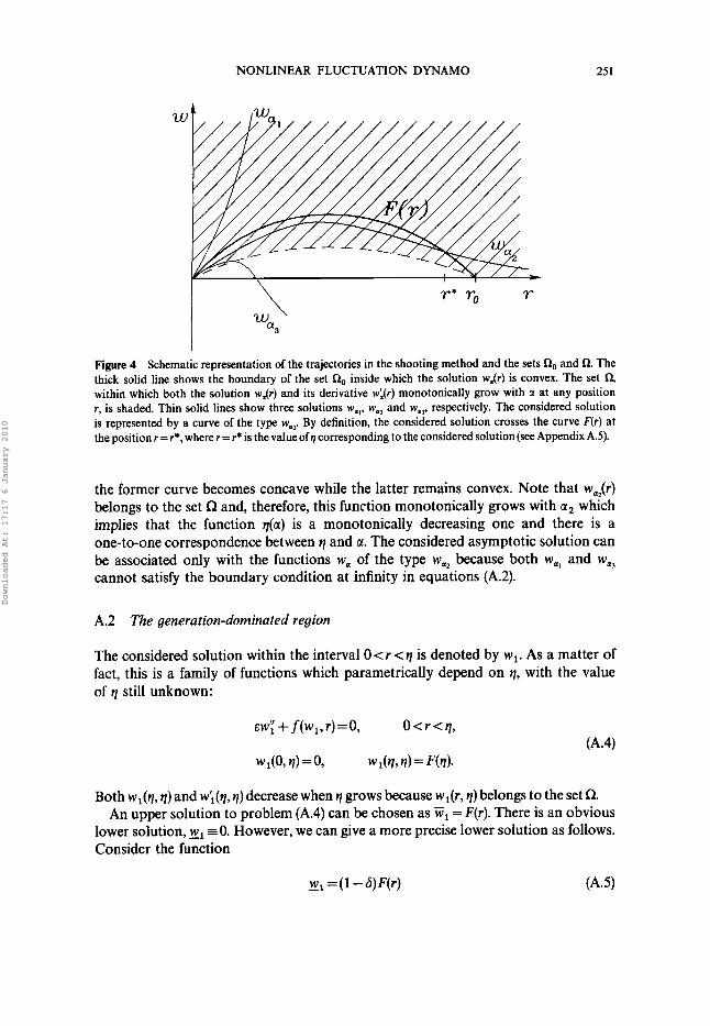
Figure 4 Schematic representation of the trajectories in the shooting method and the sets R, and R. The thick solid line shows the boundary of the set R, inside which the solution w,(r) is convex. The set t2, within which both the solution wdr) and its derivative wh(r) monotonically grow with a at any position r, is shaded. Thin solid lines show three solutions we,, we, and w,,, respectively. The considered solution is represented by a curve of the type wm2 By definition, the considered solution crosses the curve F(r) at the position r = r*, where r = r* is the value of 1 corresponding to the considered solution (see Appendix AS).

the former curve becomes concave while the latter remains convex. Note that w,Lr) belongs to the set i2 and, therefore, this function monotonically grows with ag which implies that the function q(a) is a monotonically decreasing one and there is a one-to-one correspondence between q and a. The considered asymptotic solution can be associated only with the functions w, of the type w,, because both w,, and w,, cannot satisfy the boundary condition at infinity in equations (A.2).

A.2 The generation-dominated region

The considered solution within the interval 0 < r < q is denoted by w,. As a matter of fact, this is a family of functions which parametrically depend on q, with the value of q still unknown:

Both wl(q, q) and w>(q, q) decrease when q grows because wl(r, q) belongs to the set R. An upper solution to problem (A.4) can be chosen as ts, = F(r). There is an obvious

lower solution, wl ~ 0 . However, we can give a more precise lower solution as follows. Consider the function



with some constant 6 (< 1). Taking into account that g'(O)=yb(O)=O, F"(r)<O and cE;(r) + f(w, r ) =O ( > 0) for r = q (r < q), one can show that for any value of q, which satisfies the inequality

for p > 1,

--[r~'~"(r,)g(r,)]''~y;'[1 +0(co)] for p = 1, &

6

r0-q>

- w1 given by (AS) remains a lower solution for wl(r ,q) . Here and below y r =Iyb(ro)l. It is important that 1F'I-m and lF"l+m for r+ro when p>1. Our aim is now to choose 6 and q in such a way as to obtain a lower solution which reasonably approximates the exact solution for 0 < r < q and q is close to ro. For 6 = O( 1) [more specifically, O(E')] the values of q are very close to ro but llil differs from the exact solution rather strongly [see (AS)]. For ~ = O ( E ' ) with any positive constant k, the

situation is the opposite. A reasonable choice of 6 assumes 6 = 0 - with a positive

constant k : (ld.,)

These arguments lead to the following two conclusions. First, both Zl and )411 belong to Q. As we have seen in Section A.l, the considered solution w1 belongs to the set, R and, hence, the solution is unique. Therefore, the lower and upper solutions obtained are the lower and upper bounds of the solution, respectively (see Theorem 1). Second, we have the estimate w;(q) = F'(q)[ 1 - o( l)] > F'(q) which will be used below.

A.3 The transition region

Now we turn to the interval q t r t r , where we consider the function w2(r,q) which should smoothly match the function wl(r , q) at r = q. The function wz(r, q ) is governed by an initial value problem rather than a boundary value one:

Like the function wl(r , q), the function w2(r, q) belongs to the set R and therefore monotonically decreases with q. Thus, if w2(r, q ) is singular for some q = r*, then this



is true also for any q<r*. We shall find two values of q, denoted by r* and F*, for which w2(r, q ) tends to + 00 and becomes negative, respectively, for finite or infinite r. This will imply that the desired value q = r* satisfies the inequalities L* < r* <F*. The estimates of r* and F* are given by equations (A.8) and (A.11) below.

In order to estimate 7;* we construct the lower solution of the problem (A.6). We introduce a new variable

W, = w 2 - F(r), q < r < ro.

In terms of this variable, the problem (A.6) reduces to

where

is a positive function of W, and r for W, > 0 and W2(q, q) > 0. In order to obtain the lower solution y2, one should replace in (A.7) the term

~ - ' y ~ p W , by its lower bound i , u ~ - ' y ~ ( r ~ - q ) y , , the term -F"(r) should be replaced by - F"(q) and f2 replaced by zero over the interval q < r < q +3ro - q). This yields the following

cosh{ [ E - lylp(r0 - q)/2l1l2(r- q)} - 1

PY l(r0 - _w, = - 2&F"(V)

Simultaneously, we see that _W; < W,.

In order to determine the order of _W, in E, we represent q as q = r O - ) < * ~ S with certain t* and s. This results in the following inequality

W,(r,-3t*~~)>cosh [a(&-(' -3s)/2t*3/2)] x O ( E ~ - ~ ) .

The desired value of r* is given by the following maximal value of q such that - W2+m when E+O at finite or infinite r :

In order to obtain the upper estimate of r*, denoted by 7;*, we consider the problem



(A.6) from another viewpoint. Substituting an explicit expression for f ( w , , r ) we obtain

The upper solution W2(r , q) can be given in the following implicit form

where G = r;’g(ro)[ 1 + o( l)]. The reader can verify this fact by direct substitution of this equation into equation (A.9). We intend to use the following relation which follows from the latter expression for W, by differentiation with respect to r :

1 G 1 - E ( F ~ ) ~ = - ~ ’ ; + 2 - F ” + 2 ( q ) ] + ~ ~ [ ~ ; ( q , q ) ] 2 . (A.lO) 2 P + 2

The desired estimate of F* is actually that value of q for which W2 vanishes for some r (> ro) such that r - ro = o( 1). An estimate of F* can be obtained from equation (A.10) presuming that (SS;), =+[w;(q , q)], at the position where w2(r, q) intersects the r-axis, which yields

(A. 1 1)

Thus, we have determined the interval

@*, F*) = ( ro - O( :), ro - O ( E ’ / ~ ) )

within which the considered solution w(r), if it exists, intersects the curve F(r): r*E@*, ?*).

These estimates reduce, within the accuracy of logarithmic terms in E, to the following very simple form

r* = ro - O(&lI3).

A.4 The diffusion-dominated region

Now we consider our problem for r > lo. For this purpose we consider the following



boundary value problem for w3(r, 0):

(A.12)

The considered solution w belongs to this family of functions and corresponds to a certain value of 0 (see Subsection A S below). We have w31,-,,+0 since if w 3 > C , with certain constant C, then it follows from equation (A.12) that w3 should exhibit a superexponential growth (we recall that p> 1) and the boundary condition (A.12) at infinity cannot be satisfied. Therefore, we can transform the boundary condition at r+co in equation (A.12):

w3( co,0) = 0. (A. 13)

It is obvious that solution of the problem (A.12), (A.13) is unique since it belongs to the set R. We can prove the existence of the solution by obtaining its upper and lower solutions, W3 and w,, respectively.

Let us introduce

- G = min r-”(r) = const > 0 r>ro

and consider the following problem which defines the upper solution iT3(r, 0):

whose unique solution is given by

(A.14)

(A. 15)

Using equation (A.14) one can show that solution of the problem (A.12), (A.13) satisfies the following inequality

In order to obtain the lower solution w3, we presume that there exist constants E and IC such that

i.e. g(r) grows with r no faster than an exponential function. The lower solution can



be expressed through McDonald’s function K,(x) as

Thus, the problem (A. 12) has a unique solution which obeys the following inequalities:

AS Matching the three regional solutions

Now we show that a unique solution of the problem (A.2) can be composed from the solutions w l ( r , q) and w2(r, q ) of the problems (A.4) and (A.6) and solution w3(r , 8) of the problem (A.12) by an appropriate choice of the constants q and 8. Since in the case of the second-order differential equation one should match both the functions and their derivatives, it is sufficient to show that there exist unique values of (qe) , denoted for a moment as (r*, O,), such that

We recall that w , and w2 match smoothly at r = r * by definition. Consider first the dependence of w;(ro, 8) on O[ = ~ 3 ( r o , el]. For 8 = 0 the problem

(A . 12) has only trivial solution. The value of w;(ro, 8) decreases with ~ 3 ( r o , 8 ) because for 8> 0 the function w&, 8) belongs to the set R. A plot of w;(ro, 8) as a function of w3(r, 0) is schematically shown by the dashed line in the “phase diagram” presented in Figure 5.

Consider now the dependence of w;(r,, q ) on w2(ro, q). Both these quantities decrease with q because the function wz(r ,q ) belongs to the set R. Therefore, w;(r,,q) monotonically grows with w2(ro,q). The solid line in Figure 5 runs upwards since w;<O when w2=o(1 ) , or r*=r,-o(l). Therefore, if the two phase trajectories in Figure 5 intersect, then the intersection point is unique.

What is left, is to prove that the phase diagrams for w2 and w 3 intersect (the solid and the dashed lines in Figure 5, respectively). The dashed line belongs to the region p < O where p is defined as the derivative of the corresponding function (see above). The solid line belongs to the region p < 0 when q = o( 1 ) (q is a function w itself). For instance, we have shown above that w;(r,,F*)<O. However, we have also shown that w;(ro, I*) > 0. Therefore, the dashed and the solid curves in Figure 5 inevitably intersect and the intersection point (I*, 8,) corresponds to a certain value of q = r* between r* and F*.


NONLINEAR FLUCTUATION DYNAMO

P

251

/ / 9 9

Figure 5 Matching of solutions w2(r,q) and w,(r,O) at r=r* is shown on the “phase plane” q = ~ l , , ~ , p = W ’ I , = , ~ . The dashed line shows the phase trajectory for wj (here 0 is a parameter varying along the curve shown). The solid line shows the phase trajectory for w2 with 1 as a parameter varying along the curve. The unique point at which the two curves intersect, corresponds to the desired values of parameters (r*, 0).

Thus, we have proved the existence and uniqueness of solution of the problem (A.2) for small E, which means the existence and uniqueness of solution of the problem (A. 1). The discussion above implies that E(r) is close and slightly smaller than E,(r) = [yO(r)/g(r)]’/’’ for 0 < r < r* z ro as shown in Figure 2. For E+O the solution tends to Eo(r) for r < r*. At the position r = r* = ro[l - O ( E ’ / ~ ) ] we have E(r*)= Eo(r*) and E(r) monotonically tends to zero for r+co while satisfying the estimate

The latter estimate can be derived from equation (A.15) for w o o .

APPENDIX B

Consider the boundary value problem

E(0) = 0, E(co)=O

with 1.



Similar to the approach of Section 3, we first obtain the solution valid for r>ro where yo=O, which reads

where the constant C = C(E) will be determined below.

conditions At the radius r=ro solution of the problem (B.l) should satisfy the matching

E(ro - 0) = E(ro + O), E(ro - 0) = E‘(ro + 0). (B.3)

It follows from (B.2) that

Using now (B.3) we reformulate the problem to a closed form for E over the interval (0, ro):

E(0) = 0, (rE)’l,=,o=O.

Now we introduce the variable w = Er in terms of which we have

w(0) = 0, w’(ro) = O .

Equation (B.5) can be formally represented as a linear equation of the form E W ” + Q ~ W = O with

The pair of its linearly independent solutions W, and W, have the following WKB asymptotic forms

Hence, for Q(r) = O( 1) both solutions W, and W, are rapidly oscillating functions of r and, therefore, their linear combination cannot be everywhere positive as required



by the physical meaning of the solution. The condition w(r)aO can be satisfied for O<r<ro only when Q(r)=O(&). It follows then from (B.6) that w = O ( ~ - ” p ) .

Therefore, we can represent solution of the problem (B.5) as

w(r, E ) = E - ””W(r, E).

We have the following equations for W:

W(0) = 0, W(r,) = 0.

Solution of this boundary value problem can be represented as a regular perturbation series

m

After substitution of this series into (B.7) we extract the terms of equal orders in E.

To the leading order we obtain

W~+yor’g-’W~-”=O, 0 < r < ro, (B.8)

WO(0) = 0, Wb(ro) = 0.

First we show that a non-negative solution of the problem (B.8) is unique for p 2 1. (In the main text we discuss the case p = 1 when the problem can be solved by quadratures.) In order to do this, we consider the following auxiliary boundary value problem:

WL + yor”g- W,l -” =O,

W,(O) = 0,

0 < r < lo,

03.9) W,(O) = a

with a>O. The derivative of the second term on the left-hand side of (B.9) with respect to W,

is non-positive when p > 1. The function W,(r) monotonically grows with a. Indeed, let us suppose that this is

not true, i.e. there exist al, az and R( > O ) such that a1 >az and W,,(R)< W,,(R). The smallest non-vanishing value of R is denoted as & @ # O because al >az). Then

W,,O = wu2m > Wu,(r) for O<r<R.

These relations imply that W,,@ < W@J. However, this conclusion contradicts the



fact that Wc grows with W, because Wu = a + & W;(x)dx. This proves that W,(r) grows with a. This also implies that Wu(r) grows with a.

Hence, there exists no more than one value of a for which Wh(ro) =O. The arguments above prove that solution of the problem (B.8) is unique if it exists.

In order to prove the existence of this solution, it is sufficient to give such values of a, denoted as a1 and a2, that W,,(ro)>O and Wa,(ro)<O.

First we obtain r2 . Integrating (B.9) from 0 to r we obtain

(B.lO)

As follows from (B.10), W a < a and, therefore, W, <ar. As far as p > 1, we obtain from (B.lO) that

Thus, Wa(ro)<O for O < a < T where

T = [ s,” yo(x)g- ‘ (x)x~x]~” .

The result is the lower bound for a: a2 = 7:

function W : Now we turn to the upper bound, a,. Consider the following problem for the

(B. 11)

where W,, is the solution of the problem (B.9) which corresponds to ct=a2= T.

Wa(ro)>W’(ro) = 0, is recovered when a =m’(O). This yields the upper bound a,. As far as W;,-” < W;,-”, a solution of the problem (B.9), which satisfies the inequality

Solution of the problem (B.11) can be given in the following explicit form

Therefore, we have

This completes the proof of existence and uniqueness of solution of the problem (B.8).



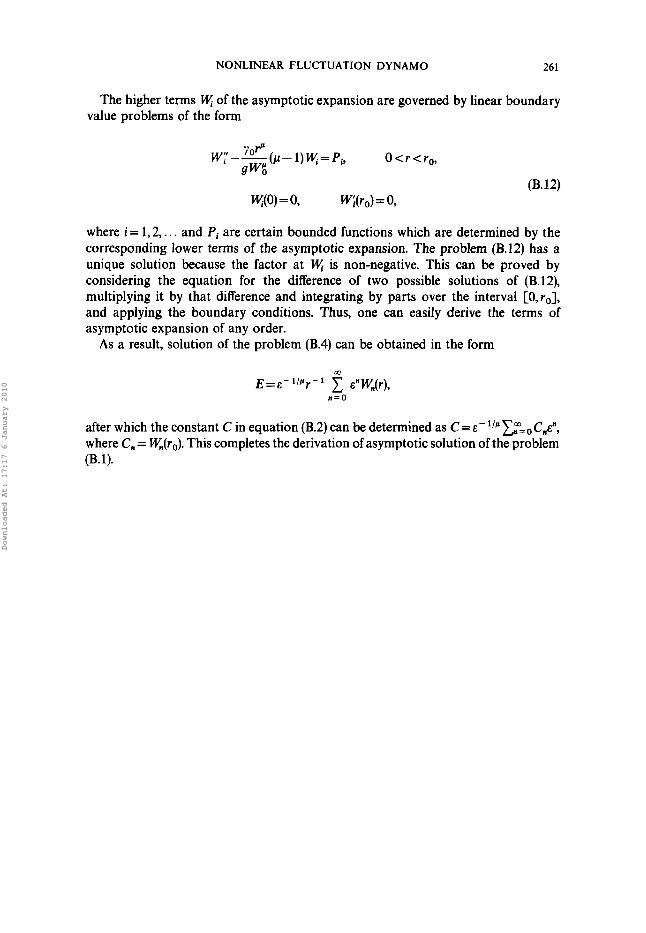
The higher terms % of the asymptotic expansion are governed by linear boundary value problems of the form

(B.12) lq(0) = 0, WXl.0) = 0,

where i = 1,2,. . . and Pi are certain bounded functions which are determined by the corresponding lower terms of the asymptotic expansion. The problem (B.12) has a unique solution because the factor at W. is non-negative. This can be proved by considering the equation for the difference of two possible solutions of (B.12), multiplying it by that difference and integrating by parts over the interval [O,r,], and applying the boundary conditions. Thus, one can easily derive the terms of asymptotic expansion of any order.

As a result, solution of the problem (B.4) can be obtained in the form

after which the constant C in equation (B.2) can be determined as C = E - ' / ~ ~ ~ = ~ C , , E " , where C, = Wn(ro). This completes the derivation of asymptotic solution of the problem (B.1).


Documents

Geophysical & Astrophysical Fluid Dynamics Simple models ...nas13/AS/1993GAFD_Belyanin_etal_Nonlinear... · To link to this Article: DOI: 10.1080/03091929308203569 URL: ... field