2.29 Numerical Fluid Mechanics Fall 2011 Lecture 23 · 2.29 Numerical Fluid Mechanics Fall 2011 – Lecture 23 . ... – Discretization of the pressure term – Conservation principles

PFJL Lecture 23, 1 Numerical Fluid Mechanics 2.29

2.29 Numerical Fluid Mechanics

Fall 2011 – Lecture 23 REVIEW Lectures 22: • Complex Geometries • Grid Generation

– Basic concepts and structured grids • Stretched grids • Algebraic methods • General coordinate transformation • Differential equation methods • Conformal mapping methods

– Unstructured grid generation • Delaunay Triangulation • Advancing Front method

• Finite Volume on Complex geometries – Computation of convective fluxes – Computation of diffusive fluxes – Comments on 3D


TODAY (Lecture 23):

Grid Generation (end), FV on Complex Geometries

and Solution to the Navier-Stokes Equations • Grid Generation

– Basic concepts and structured grids • Algebraic methods (stretched grids), General coordinate transformation, Differential

equation methods, Conformal mapping methods

– Unstructured grid generation • Delaunay Triangulation • Advancing Front method

• Finite Volume on Complex geometries – Computation of convective fluxes – Computation of diffusive fluxes – Comments on 3D

• Solution of the Navier-Stokes Equations – Discretization of the convective and viscous terms – Discretization of the pressure term – Conservation principles


References and Reading Assignments

• Chapter 8 on “Complex Geometries” and Chapter 7 on “Incompressible Navier-Stokes equations” of “J. H. Ferziger and M. Peric, Computational Methods for Fluid Dynamics. Springer, NY, 3rd edition, 2002”

• Chapter 9 on “Grid Generation” and Chapter 11 on “Incompressible Navier-Stokes Equations” of T. Cebeci, J. P. Shao, F. Kafyeke and E. Laurendeau, Computational Fluid Dynamics for Engineers. Springer, 2005.

• Chapter 13 on “Grid Generation” and Chapter 17 on “Incompressible Viscous Flows” of Fletcher, Computational Techniques for Fluid Dynamics. Springer, 2003.

• Ref on Grid Generation only:

– Thompson, J.F., Warsi Z.U.A. and C.W. Mastin, “Numerical Grid Generation, Foundations and Applications”, North Holland, 1985


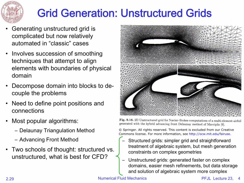
Grid Generation: Unstructured Grids

• Generating unstructured grid is

complicated but now relatively

automated in “classic” cases

• Involves succession of smoothing

techniques that attempt to align

elements with boundaries of physical

domain

• Decompose domain into blocks to de-

couple the problems

• Need to define point positions and

connections

• Most popular algorithms:

– Delaunay Triangulation Method

– Advancing Front Method

• Two schools of thought: structured vs.

unstructured, what is best for CFD?

– Structured grids: simpler grid and straightforward treatment of algebraic system, but mesh generation constraints on complex geometries

– Unstructured grids: generated faster on complex domains, easier mesh refinements, but data storage and solution of algebraic system more complex

© Springer. All rights reserved. This content is excluded from our Creative

Commons license. For more information, see http://ocw.mit.edu/fairuse.

http://ocw.mit.edu/fairuse

P

1 2

34

5



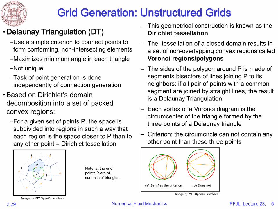
•Delaunay Triangulation (DT Dirichlet tessellation

–Use a simple criterion to connect points to – The tessellation of a closed domain results in form conforming, non-intersecting elements a set of non-overlapping convex regions called

–Maximizes minimum angle in each triangle Voronoi regions/polygons

–Not unique – The sides of the polygon around P is made of –Task of point generation is done segments bisectors of lines joining P to its

independently of connection generation neighbors: if all pair of points with a common segment are joined by straight lines, the result

• Based on Dirichlet’s domain is a Delaunay Triangulation decomposition into a set of packed

– Each vortex of a Voronoi diagram is the convex regions: circumcenter of the triangle formed by the

–For a given set of points P, the space is three points of a Delaunay triangle subdivided into regions in such a way that

–each region is the space closer to P than to Criterion: the circumcircle can not contain any any other point = Dirichlet tessellation

– This geometrical construction is known as the )

other point than these three points

Note: at the end, points P are at summits of triangles

(a) Satisfies the criterion (b) Does not

Image by MIT OpenCourseWare.Image by MIT OpenCourseWare.



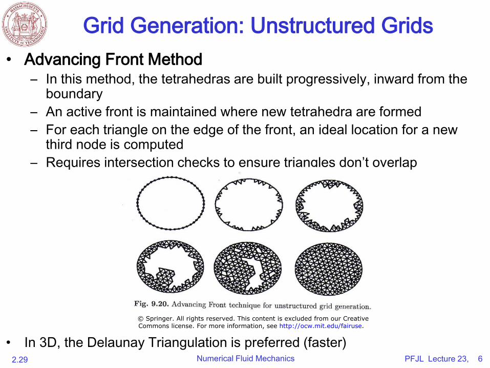
• Advancing Front Method – In this method, the tetrahedras are built progressively, inward from the

boundary

– An active front is maintained where new tetrahedra are formed

– For each triangle on the edge of the front, an ideal location for a new third node is computed

– Requires intersection checks to ensure triangles don’t overlap

• In 3D, the Delaunay Triangulation is preferred (faster)

© Springer. All rights reserved. This content is excluded from our CreativeCommons license. For more information, see http://ocw.mit.edu/fairuse.

http://ocw.mit.edu/fairuse

Finite Volumes on Complex geometries

• FD method (classic):

– Use structured-grid transformation (either algebraic-transfinite, general,

differential or conformal mapping)

– Solve transformed equations on simple orthogonal computational domain

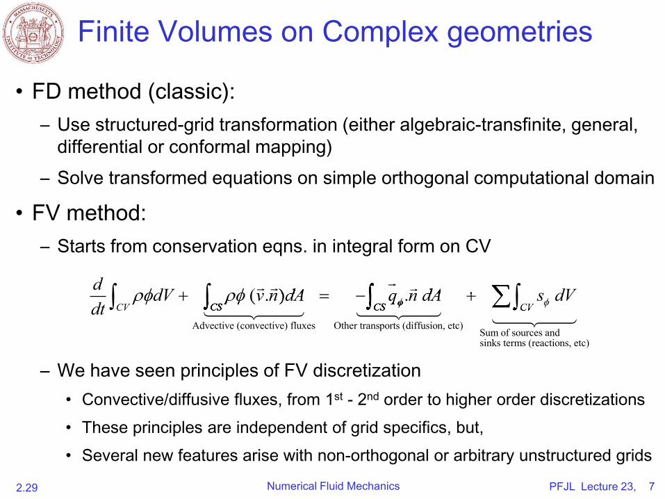
• FV method:

– Starts from conservation eqns. in integral form on CV

– We have seen principles of FV discretization

• Convective/diffusive fluxes, from 1st - 2nd order to higher order discretizations

• These principles are independent of grid specifics, but,

• Several new features arise with non-orthogonal or arbitrary unstructured grids

2.29 Numerical Fluid Mechanics PFJL Lecture 23, 7

Advective (convective) fluxes Other transports (diffusion, etc)Sum of sources andsinks terms (reactions, etc)

( . ) .CV CS CS CV

d dV v n dA q n dA s dVdt dV v n dA q n dA( . )dV v n dA q n dA( . ) dV v n dA q n dAdV v n dA q n dAdV v n dA q n dA

CS CSdV v n dA q n dA( . )dV v n dA q n dA( . )

CSdV v n dA q n dA

CS dV v n dA q n dA dV v n dA q n dA CS

CS

dV v n dA q n dA dV v n dA q n dACS

dV v n dA q n dACS

CS

dV v n dA q n dACS CS CS

CS

CS CS

CS

dV v n dA q n dA dV v n dA q n dA dV v n dA q n dA dV v n dA q n dACS

dV v n dA q n dACS

CS

dV v n dA q n dACS CS

dV v n dA q n dACS

CS

dV v n dA q n dACS CSCS

dV v n dA q n dAdV v n dA q n dACS

dV v n dA q n dACSCS

dV v n dA q n dACS CVCVCV


Expressing fluxes at the surface based on cell-averaged (nodal)

values: Summary of Two Approaches and Boundary Conditions

• Set-up of surface/volume integrals: 2 approaches (do things in opposite order)

1. (i) Evaluate integrals using classic rules (symbolic evaluation); (ii) Then, to obtain the unknown symbolic values, interpolate based on cell-averaged (nodal) values

Similar for other integrals:

2. (i) Select shape of solution within CV (piecewise approximation); (ii) impose volume constraints to express coefficients in terms of nodal values; and (iii) then integrate. (this approach was used in the examples).

Similar for higher dimensions:

• Boundary conditions:

– Directly imposed for convective fluxes

– One-side differences for diffusive fluxes

( ) ( ) ( )( ) ( )( ) ( )

( ' )

( )

i i

i Pi

P

Pe

a a

aa P

e PV

e S

i x xx xii x

F s

iii F f dA

J

F

1( , , )V V

S s dV dV etcV

( ) ( )( ' )

( ) ( ' ) ( ' )e

e e eSe P

e P P

i F f dA FF s

ii s s

GF

H H

( , ) ( , );

( , ) ;i

i

a

a P P P

x y x y etc

x y etc

J

(From lecture 19)


Approx. of Surface/Volume Integrals:

Classic symbolic formulas

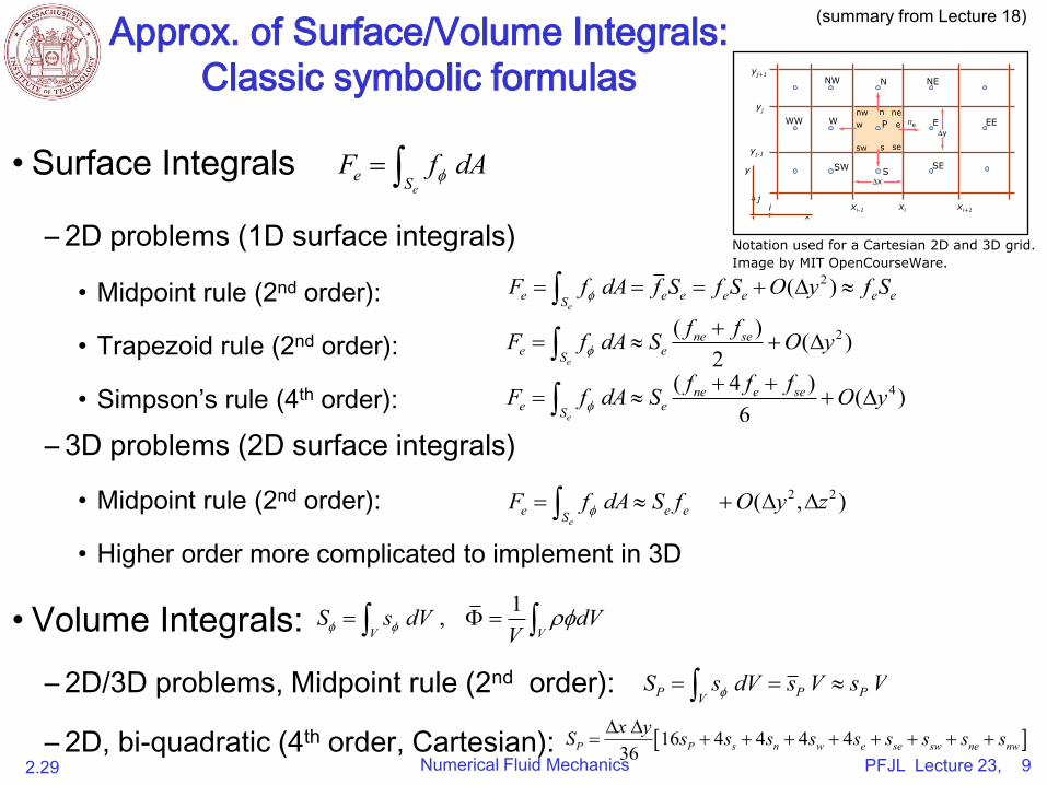
• Surface Integrals

– 2D problems (1D surface integrals)

• Midpoint rule (2nd order):

• Trapezoid rule (2nd order):

• Simpson’s rule (4th order):

3D problems (2D surface integr

• Midpoint rule (2nd order):

• Higher order more complicated t

– als)

o implement in 3D

• Volume Integrals:

– 2D/3D problems, Midpoint rule (2nd order):

– 2D, bi-quadratic (4th order, Cartesian):

2( )e

e e e e e e eSF f dA f S f S O y f S

2( ) ( )2e

ne see eS

f fF f dA S O y

4( 4 ) ( )6e

ne e see eS

f f fF f dA S O y

ee S

F f dA

2 2( , )e

e e eSF f dA S f O y z

P P PVS s dV s V s V

16 4 4 4 436P P s n w e se sw ne nwx yS s s s s s s s s s

1,V V

S s dV dVV

(summary from Lecture 18)

yj+1

xi-1 xi xi+1

yj-1

y

ji

x

yj

NW

WW W

SW S SE

E EE

N NE

∆y

∆x

nw

s

nw neneP

sw se

e

Notation used for a Cartesian 2D and 3D grid. Image by MIT OpenCourseWare.

PFJL Lecture 23, 10Numerical Fluid Mechanics 2.29

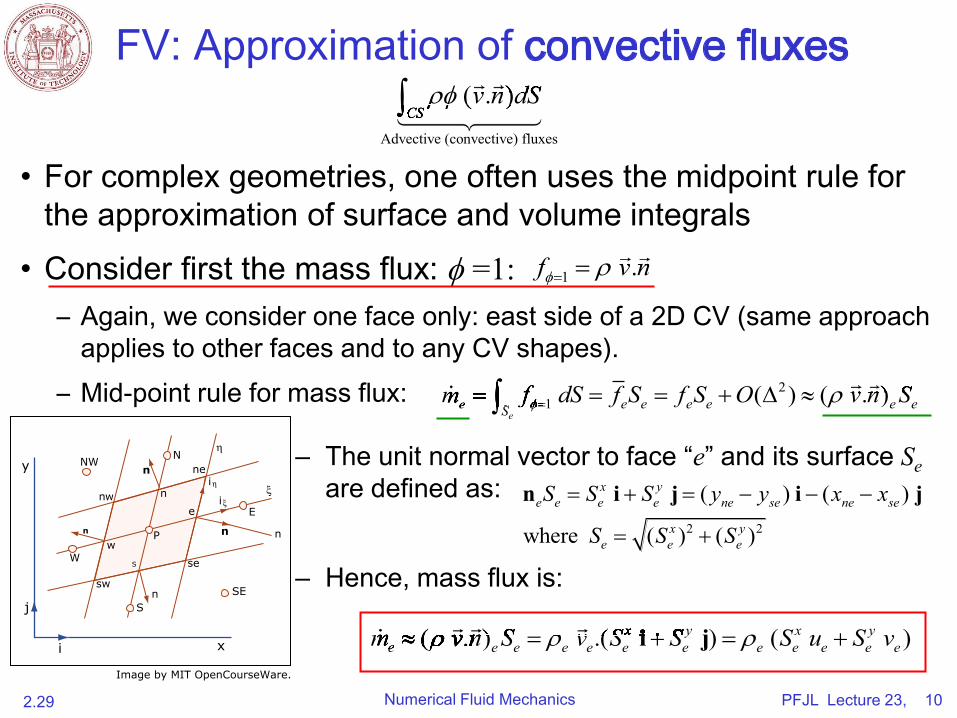
FV: Approximation of convective fluxes

• For complex geometries, one often uses the midpoint rule for

the approximation of surface and volume integrals

• Consider first the mass flux: =1: f1 v n.

– Again, we consider one face only: east side of a 2D CV (same approach

applies to other faces and to any CV shapes).

– Mid-point rule for mass flux: m f 2e 1 dS f Se e f Se e O( ) ( v. )n e eS

( .v n)dSCS

Advective (convective) fluxes

FV: Approximation of v n dS( . )v n dS( . )( . )

CSCSCS

f v n

– The unit normal vector to face “e” and its surface Seare defined as: n S S x S y

e e e i je ( yne yse ) (i j xne xse )

where S S x y2 2e e ( ) (Se )

– Hence, mass flux is:

m x y x ye ( v n. )e eS e ve.(Se i j Se ) e (Se ue Se ve)

eSm f dS f S f S O v n S( ) ( . )m f dS f S f S O v n S( ) ( . )m f dS f S f S O v n Sm f dS f S f S O v n Sem f dS f S f S O v n Sem f dS f S f S O v n SS

m f dS f S f S O v n SS

m f dS f S f S O v n Sm f dS f S f S O v n Sm f dS f S f S O v n Sm f dS f S f S O v n Sm f dS f S f S O v n S m f dS f S f S O v n Sm f dS f S f S O v n Sm f dS f S f S O v n S m f dS f S f S O v n Sm f dS f S f S O v n Sm f dS f S f S O v n S m f dS f S f S O v n Sm f dS f S f S O v n Sm f dS f S f S O v n SS

m f dS f S f S O v n SSSm f dS f S f S O v n SS

m f dS f S f S O v n S m f dS f S f S O v n Sm f dS f S f S O v n S m f dS f S f S O v n S

( . ) .( ) ( )x y( . ) .( ) ( )x y( . ) .( ) ( )( . ) .( ) ( )m v n S v S S S u S v( . ) .( ) ( )( . ) .( ) ( )x y( . ) .( ) ( )m v n S v S S S u S v( . ) .( ) ( )x y( . ) .( ) ( )( . ) .( ) ( )m v n S v S S S u S v( . ) .( ) ( ) ( . ) .( ) ( )m v n S v S S S u S v( . ) .( ) ( )( . ) .( ) ( )x y( . ) .( ) ( )m v n S v S S S u S v( . ) .( ) ( )x y( . ) .( ) ( ) ( . ) .( ) ( )x y( . ) .( ) ( )m v n S v S S S u S v( . ) .( ) ( )x y( . ) .( ) ( )( . ) .( ) ( )m v n S v S S S u S v( . ) .( ) ( ) ( . ) .( ) ( )m v n S v S S S u S v( . ) .( ) ( ) ( . ) .( ) ( )m v n S v S S S u S v( . ) .( ) ( ) ( . ) .( ) ( )m v n S v S S S u S v( . ) .( ) ( )( . ) .( ) ( )x y( . ) .( ) ( )i j( . ) .( ) ( )x y( . ) .( ) ( )( . ) .( ) ( )x y( . ) .( ) ( )m v n S v S S S u S v( . ) .( ) ( )x y( . ) .( ) ( )i j( . ) .( ) ( )x y( . ) .( ) ( )m v n S v S S S u S v( . ) .( ) ( )x y( . ) .( ) ( )( . ) .( ) ( )x y( . ) .( ) ( )m v n S v S S S u S v( . ) .( ) ( )x y( . ) .( ) ( ) ( . ) .( ) ( )x y( . ) .( ) ( )m v n S v S S S u S v( . ) .( ) ( )x y( . ) .( ) ( )i j( . ) .( ) ( )x y( . ) .( ) ( )m v n S v S S S u S v( . ) .( ) ( )x y( . ) .( ) ( ) ( . ) .( ) ( )x y( . ) .( ) ( )m v n S v S S S u S v( . ) .( ) ( )x y( . ) .( ) ( )( . ) .( ) ( )em v n S v S S S u S v( . ) .( ) ( )m v n S v S S S u S v( . ) .( ) ( )em v n S v S S S u S ve ( . ) .( ) ( ) ( . ) .( ) ( )( . ) .( ) ( )m v n S v S S S u S v( . ) .( ) ( ) ( . ) .( ) ( )m v n S v S S S u S v( . ) .( ) ( )m v n S v S S S u S v m v n S v S S S u S v( . ) .( ) ( )m v n S v S S S u S v( . ) .( ) ( ) ( . ) .( ) ( )m v n S v S S S u S v( . ) .( ) ( )( . ) .( ) ( )m v n S v S S S u S v( . ) .( ) ( ) ( . ) .( ) ( )m v n S v S S S u S v( . ) .( ) ( ) ( . ) .( ) ( )m v n S v S S S u S v( . ) .( ) ( ) ( . ) .( ) ( )m v n S v S S S u S v( . ) .( ) ( )( . ) .( ) ( )( . ) .( ) ( )m v n S v S S S u S v( . ) .( ) ( )( . ) .( ) ( )m v n S v S S S u S v( . ) .( ) ( ) ( . ) .( ) ( )m v n S v S S S u S v( . ) .( ) ( )( . ) .( ) ( )m v n S v S S S u S v( . ) .( ) ( ) ( . ) .( ) ( )m v n S v S S S u S v( . ) .( ) ( ) ( . ) .( ) ( )m v n S v S S S u S v( . ) .( ) ( ) ( . ) .( ) ( )m v n S v S S S u S v( . ) .( ) ( )

W

sw

Sn

x

SE

se

E

Nn

n n

n

n

ne

P

nw

NW

w

η

iη

iξξ

e

y

i

j

S

Image by MIT OpenCourseWare.

W

sw

Sn

x

SE

se

E

Nn

n n

n

n

ne

P

nw

NW

w

η

iη

iξξ

e

y

i

j

S

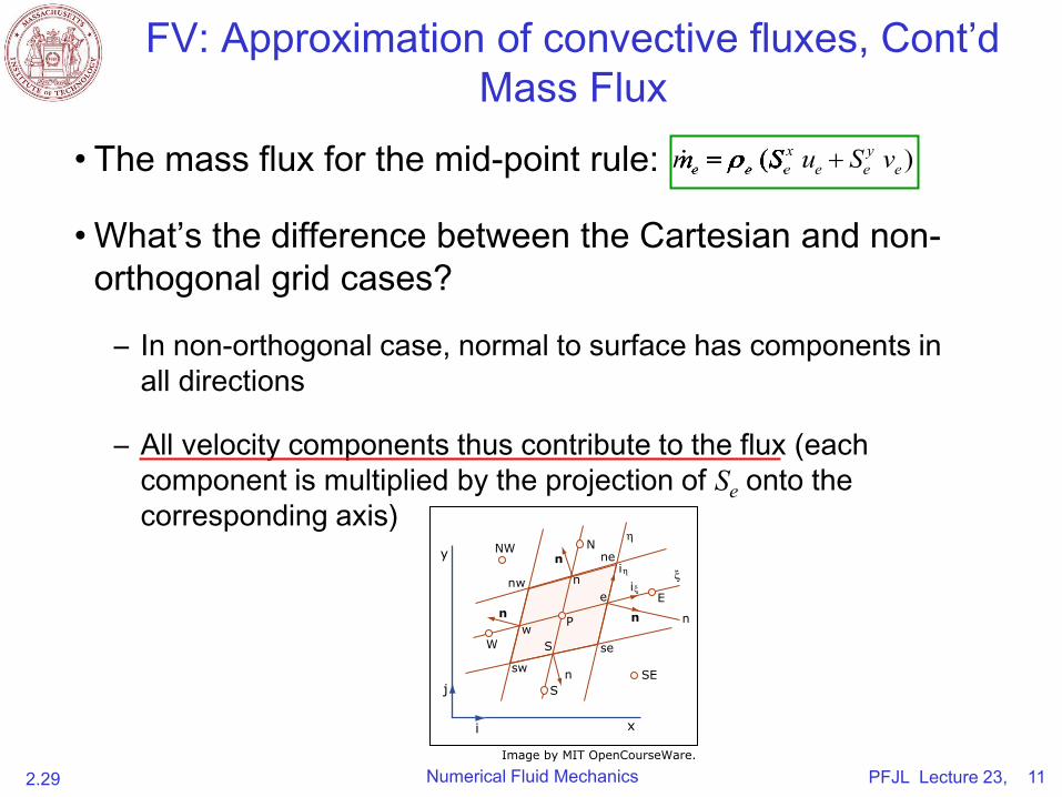
FV: Approximation of convective fluxes, Cont’d

Mass Flux

• The mass flux for the mid-point rule: m ( x ye e S ue e Se ev

• What’s the difference between the Cartesian and non-

orthogonal grid cases?

– In non-orthogonal case, normal to surface has components in

all directions

– All velocity components thus contribute to the flux (each

component is multiplied by the projection of onto the Secorresponding axis)


)( )e e e e e em S u S v( )m S u S v( )e e e e e em S u S ve e e e e ee e e e e e( )e e e e e e( )m S u S v( )m S u S v( )e e e e e em S u S ve e e e e e( )e e e e e e( )m S u S v( )e e e e e e( )e e e e e ee e e e e em S u S vm S u S ve e e e e em S u S ve e e e e ee e e e e em S u S ve e e e e em S u S v m S u S v( )m S u S v( ) ( )m S u S v( )m S u S vm S u S v m S u S vm S u S v


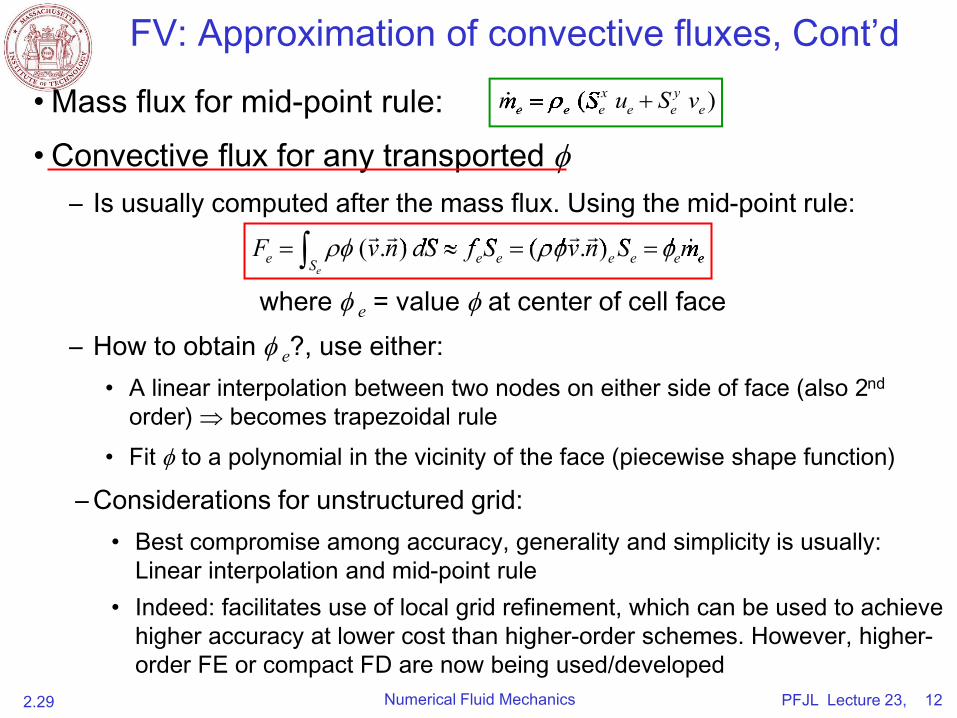
FV: Approximation of convective fluxes, Cont’d

• Mass flux for mid-point rule:

• Convective flux for any transported

– Is usually computed after the mass flux. Using the mid-point rule:

where = value at center of cell face e

– How to obtain ?, use either: e

• A linear interpolation between two nodes on either side of face (also 2nd

order) becomes trapezoidal rule

• Fit to a polynomial in the vicinity of the face (piecewise shape function)

– Considerations for unstructured grid:

• Best compromise among accuracy, generality and simplicity is usually:

Linear interpolation and mid-point rule

• Indeed: facilitates use of local grid refinement, which can be used to achieve

higher accuracy at lower cost than higher-order schemes. However, higher-

order FE or compact FD are now being used/developed


( . ) ( . )e

e e e e e e eSF v n dS f S v n S m F v n dS f S v n S m( . ) ( . )F v n dS f S v n S m( . ) ( . )F v n dS f S v n S m F v n dS f S v n S m( . ) ( . )F v n dS f S v n S m( . ) ( . ) ( . ) ( . )F v n dS f S v n S m( . ) ( . )( . ) ( . )F v n dS f S v n S m( . ) ( . ) ( . ) ( . )F v n dS f S v n S m( . ) ( . )F v n dS f S v n S m F v n dS f S v n S m F v n dS f S v n S m F v n dS f S v n S m( . ) ( . )F v n dS f S v n S m( . ) ( . ) ( . ) ( . )F v n dS f S v n S m( . ) ( . ) ( . ) ( . )F v n dS f S v n S m( . ) ( . ) ( . ) ( . )F v n dS f S v n S m( . ) ( . )e e e eF v n dS f S v n S me e e eF v n dS f S v n S me e e eF v n dS f S v n S m

( )x ye e e e e em S u S v ( )e e e e e em S u S v( )m S u S v( )e e e e e em S u S ve e e e e ee e e e e e( )e e e e e e( )m S u S v( )m S u S v( )e e e e e em S u S ve e e e e e( )e e e e e e( )m S u S v( )e e e e e e( )e e e e e ee e e e e em S u S vm S u S ve e e e e em S u S ve e e e e ee e e e e em S u S ve e e e e em S u S v m S u S v( )m S u S v( ) ( )m S u S v( )m S u S vm S u S v m S u S vm S u S v


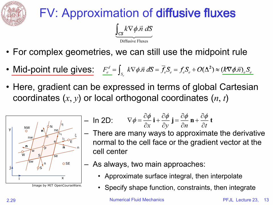
FV: Approximation of diffusive fluxes

– In 2D: i j

n t

x y n t– There are many ways to approximate the derivative

normal to the cell face or the gradient vector at the cell center

– As always, two main approaches: • Approximate surface integral, then interpolate

• Specify shape function, constraints, then integrate

2F k n dS f S f S O k n S2F k n dS f S f S O k n S2( ) ( . )F k n dS f S f S O k n S( ) ( . )F k n dS f S f S O k n S F k n dS f S f S O k n S( ) ( . )F k n dS f S f S O k n S( ) ( . ) ( ) ( . )F k n dS f S f S O k n S( ) ( . )2( ) ( . )2F k n dS f S f S O k n S2( ) ( . )2 2( ) ( . )2F k n dS f S f S O k n S2( ) ( . )2F k n dS f S f S O k n S F k n dS f S f S O k n S F k n dS f S f S O k n S F k n dS f S f S O k n S( ) ( . )F k n dS f S f S O k n S( ) ( . ) ( ) ( . )F k n dS f S f S O k n S( ) ( . ) ( ) ( . )F k n dS f S f S O k n S( ) ( . ) ( ) ( . )F k n dS f S f S O k n S( ) ( . )2( ) ( . )2F k n dS f S f S O k n S2( ) ( . )2 2( ) ( . )2F k n dS f S f S O k n S2( ) ( . )2 2( ) ( . )2F k n dS f S f S O k n S2( ) ( . )2 2( ) ( . )2F k n dS f S f S O k n S2( ) ( . )2

k n dS .CS

Diffusive Fluxes

• For complex geometries, we can still use the midpoint rule

• Mid-point rule gives: F de k.n dS f Se e f S 2

e e O( ) (k . )n e eSSe

• Here, gradient can be expressed in terms of global Cartesian

coordinates (x, y) or local orthogonal coordinates (n, t)

k n dSCS

CSCS

W

sw

Sn

x

SE

se

E

Nn

n n

n

n

ne

P

nw

NW

w

η

iη

iξξ

e

y

i

j

S



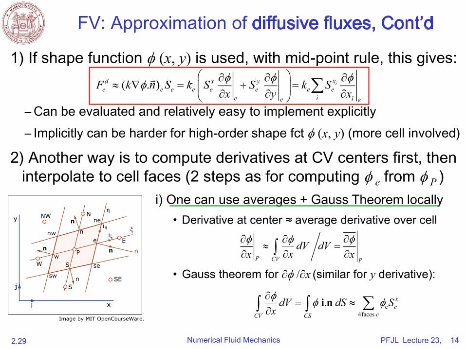
FV: Approximation of diffusive fluxes, Cont’d

1) If shape function (x, y) is used, with mid-point rule, this gives:

F d x ye (k n. )e eS ke Se Se k S x

i

x y e e e e i xi e

– Can be evaluated and relatively easy to implement explicitly

– Implicitly can be harder for high-order shape fct (x, y) (more cell involved)

2) Another way is to compute derivatives at CV centers first, then

interpolate to cell faces (2 steps as for computing from ) e P

i) One can use averages + Gauss Theorem locally • Derivative at center ≈ average derivative over cell

dV dV

x xP CV xP

• Gauss theorem for ∂ /∂x (similar for y derivative):

dV x i.n dS cScCV x CS 4faces c

F k n S k S S k S( . )F k n S k S S k S( . )F k n S k S S k S F k n S k S S k S( . )F k n S k S S k S( . ) ( . )F k n S k S S k S( . )

W

sw

Sn

x

SE

se

E

Nn

n n

n

n

ne

P

nw

NW

w

η

iη

iξξ

e

y

i

j

S


W

sw

Sn

x

SE

se

E

Nn

n n

n

n

ne

P

nw

NW

w

η

iη

iξξ

e

y

i

j

S



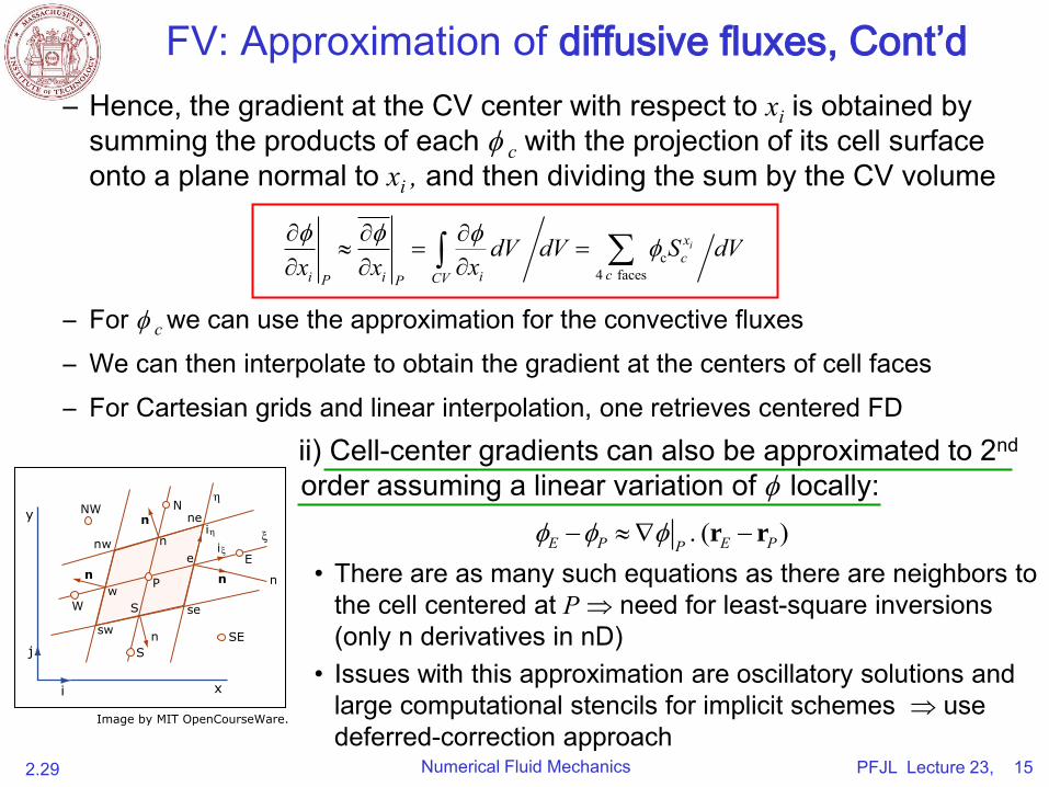
– Hence, the gradient at the CV center with respect to x is obtained by isumming the products of each with the projection of its cell surface conto a plane normal to x , and then dividing the sum by the CV volume i

– For we can use the approximation for the convective fluxes c

– We can then interpolate to obtain the gradient at the centers of cell faces

– For Cartesian grids and linear interpolation, one retrieves centered FD

ii) Cell-center gradients can also be approximated to 2nd order assuming a linear variation of locally:

• There are as many such equations as there are neighbors to

the cell centered at P need for least-square inversions (only n derivatives in nD)

• Issues with this approximation are oscillatory solutions and large computational stencils for implicit schemes use deferred-correction approach

c4 faces

ixc

cii i CVP P

dV dV S dVxx x

PE P . (r rE P )




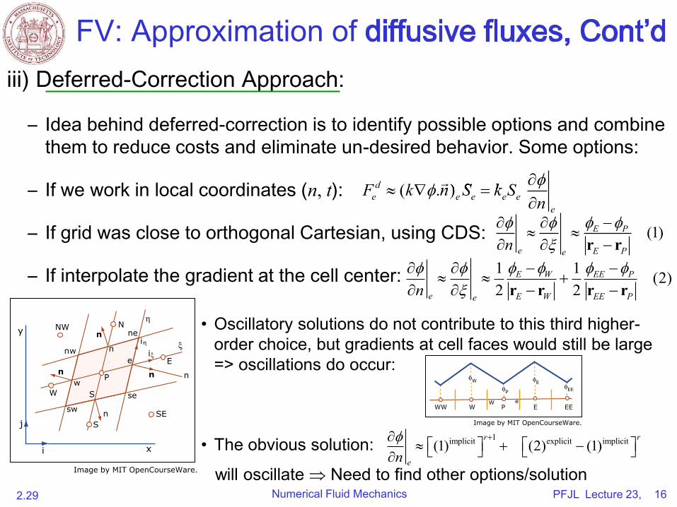
iii) Deferred-Correction Approach:

– Idea behind deferred-correction is to identify possible options and combine

them to reduce costs and eliminate un-desired behavior. Some options:

F d e (k . )n e Se k Se e

n e

ian, using CDS: E P (1) n e e r rE P

1 enter: E W 1 EE P (2) n e e 2 r rE W 2 rEE rP

– If we work in local coordinates (n, t):

– If grid was close to orthogonal Cartes

– If interpolate the gradient at the cell c

F k n S k S( . )F k n S k S( . )F k n S k S F k n S k S( . )F k n S k S( . ) ( . )F k n S k S( . )

1implicit explicit implicit(1) (2) (1)r r

en

• Oscillatory solutions do not contribute to this third higher-order choice, but gradient=> oscillations do occur:

s at cell faces would still be large

• The obvious solution:

will oscillate Need to find other options/solution

W

sw

Sn

x

SE

se

E

Nn

n n

n

n

ne

P

nw

NW

w

η

iη

iξξ

e

y

i

j

SWW W

W eP E EE

φW

φP

φEφEE





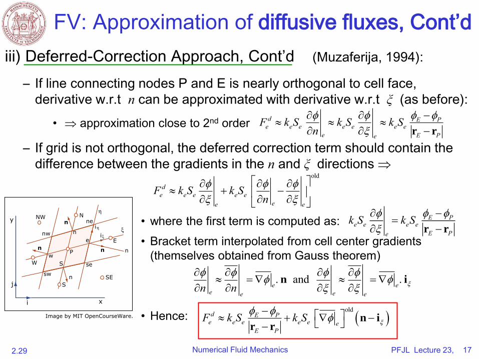
iii) Deferred-Correction Approach, Cont’d (Muzaferija, 1994):

– If line connecting nodes P and E is nearly orthogonal to cell face,

derivative w.r.t n can be approximated with derivative w.r.t ξ (as before):

• approximation close to 2nd order

– If grid is not orthogonal, the deferred correction term should contain the

difference between the gradients in the and directions n ξ

d E Pe e e e e e e

e E Pe

F k S k S k Sn

r r

• where the first term is computed as:

• Bracket term interpolated from cell center gradients (themselves obtained from Gauss theorem)

• Hence:

de e e e e

ee

F k S k Sn

old

e

. and .e

e en n

n

ee e

i

E Pe e e e e

E P

k S k S

n ir r

de

oldF

E Pe e e e

E Pe

k S k S

r r

W

sw

Sn

x

SE

se

E

Nn

n n

n

n

ne

P

nw

NW

w

η

iη

iξξ

e

y

i

j

S


W

sw

Sn

x

SE

se

E

Nn

n n

n

n

ne

P

nw

NW

w

η

iη

iξξ

e

y

i

j

S



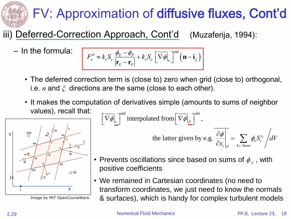
iii) Deferred-Correction Approach, Cont’d (Muzaferija, 1994):

– In the formula:

• The deferred correction term is (close to) zero when grid (close to) orthogonal,

i.e. n and ξ directions are the same (close to each other).

• It makes the computation of derivatives simple (amounts to sums of neighbor

values), recall that:

• Prevents oscillations since based on sums of c , with

positive coefficients

• We remained in Cartesian coordinates (no need to

transform coordinates, we just need to know the normals

& surfaces), which is handy for complex turbulent models

old old

interpolated from , e P

the latter given by e.g. cS

xic dV

xi 4 c facesP

old

d E Pe e e e e e

E P

F k S k S

n ir r



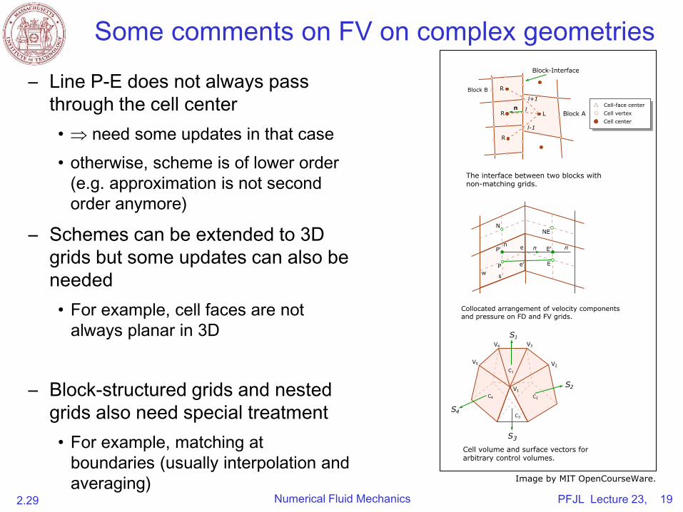
Some comments on FV on complex geometries

– Line P-E does not always pass

through the cell center

• need some updates in that case

• otherwise, scheme is of lower order

(e.g. approximation is not second

order anymore)

– Schemes can be extended to 3D

grids but some updates can also be

needed

• For example, cell faces are not

always planar in 3D

– Block-structured grids and nested

grids also need special treatment

• For example, matching at

boundaries (usually interpolation and

averaging)

S1

S2

S3

V1

V2C1

C2

C3

C4

V3V4

V5

S4

Cell volume and surface vectors for arbitrary control volumes.

w s

P

e

e'

nP'

NNE

n nE'

E

Collocated arrangement of velocity componentsand pressure on FD and FV grids.

Block A

Block B

Block-Interface

L

l+1

l-1

R

R

R

n lCell-face centerCell vertexCell center

The interface between two blocks with non-matching grids.


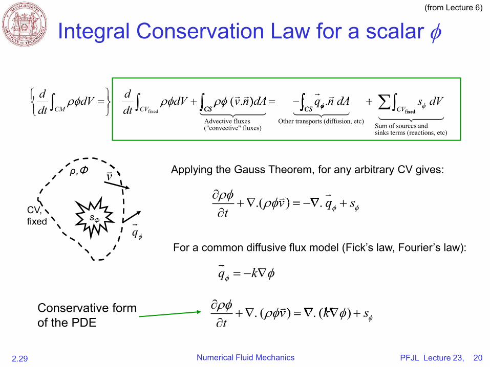
Integral Conservation Law for a scalar


fixed fixed

Advective fluxes Other transports (diffusion, etc)Sum of sources and("convective" fluxes)sinks terms (reactions, et

( . ) .CM CV CS CS CV

d ddV dV v n dA q n dA s dVdt dt

dV v n dA q n dA( . )dV v n dA q n dA( . ) dV v n dA q n dA dV v n dA q n dA dV v n dA q n dA dV v n dA q n dA

CS CSdV v n dA q n dA( . )dV v n dA q n dA( . )

CS

CSdV v n dA q n dA dV v n dA q n dA

CSdV v n dA q n dA

CS

CSdV v n dA q n dA

CS CS CS

CS

CS CS

CSdV v n dA q n dA dV v n dA q n dA dV v n dA q n dA dV v n dA q n dA

CSdV v n dA q n dA

CS

CSdV v n dA q n dA

CS CSdV v n dA q n dA

CS

CSdV v n dA q n dA

CS CS CSdV v n dA q n dA dV v n dA q n dA

CSdV v n dA q n dA

CS CSdV v n dA q n dA

CS dV v n dA q n dA dV v n dA q n dA dV v n dA q n dA dV v n dA q n dA

c)

fixedCVfixedCVfixed CV CV

. ( ) . ( )v k st

. ( ) . ( )v k s. ( ) . ( ). ( ) . ( )v k s. ( ) . ( ) . ( ) . ( )v k s. ( ) . ( ). ( ) . ( )v k s. ( ) . ( ) . ( ) . ( )v k s. ( ) . ( ) . ( ) . ( )v k s. ( ) . ( ) . ( ) . ( )v k s. ( ) . ( )

CV, fixed sΦ

q

ρ,Φ vv

.( ) .v q st

.( ) ..( ) ..( ) . .( ) . .( ) .v q s v q s.( ) .v q s.( ) . .( ) .v q s.( ) ..( ) ..( ) . .( ) ..( ) ..( ) .v q s.( ) ..( ) .v q s.( ) . .( ) .v q s.( ) ..( ) .v q s.( ) .

Applying the Gauss Theorem, for any arbitrary CV gives:

For a common diffusive flux model (Fick’s law, Fourier’s law):

q k q k

Conservative form of the PDE

(from Lecture 6)

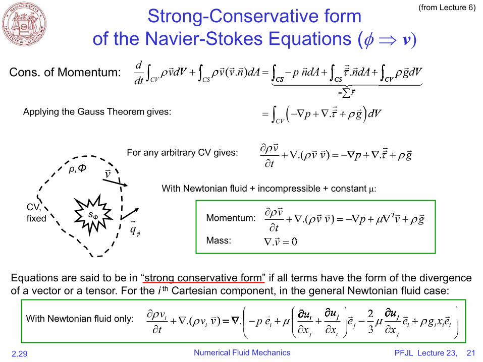
Strong-Conservative form

of the Navier-Stokes Equations ( v)


CV, fixed sΦ

q

ρ,Φ vv.( ) .v v v p g

t

v .( ) .v v p g v v p g v v p g .( ) . .( ) .v v p g v v p g.( ) .v v p g.( ) . .( ) .v v p g.( ) . v v p g v v p g v v p g v v p g .( ) .v v p g.( ) . .( ) .v v p g.( ) ..( ) ..( ) . .( ) ..( ) .v v p g.( ) . .( ) .v v p g.( ) .

Applying the Gauss Theorem gives:

Equations are said to be in “strong conservative form” if all terms have the form of the divergence of a vector or a tensor. For the i th Cartesian component, in the general Newtonian fluid case:

( . ) .

.

CV CS CS CS CV

F

CV

d vdV v v n dA p ndA ndA gdVdt

p g dV

F

vdV v v n dA p ndA ndA gdVvdV v v n dA p ndA ndA gdV vdV v v n dA p ndA ndA gdV vdV v v n dA p ndA ndA gdV vdV v v n dA p ndA ndA gdV( . )vdV v v n dA p ndA ndA gdV( . ) ( . )vdV v v n dA p ndA ndA gdV( . )vdV v v n dA p ndA ndA gdV vdV v v n dA p ndA ndA gdV vdV v v n dA p ndA ndA gdV vdV v v n dA p ndA ndA gdVvdV v v n dA p ndA ndA gdV vdV v v n dA p ndA ndA gdV vdV v v n dA p ndA ndA gdV vdV v v n dA p ndA ndA gdVvdV v v n dA p ndA ndA gdVvdV v v n dA p ndA ndA gdV vdV v v n dA p ndA ndA gdVvdV v v n dA p ndA ndA gdVvdV v v n dA p ndA ndA gdV vdV v v n dA p ndA ndA gdVvdV v v n dA p ndA ndA gdV vdV v v n dA p ndA ndA gdV vdV v v n dA p ndA ndA gdV vdV v v n dA p ndA ndA gdVvdV v v n dA p ndA ndA gdV vdV v v n dA p ndA ndA gdVvdV v v n dA p ndA ndA gdV vdV v v n dA p ndA ndA gdV vdV v v n dA p ndA ndA gdV vdV v v n dA p ndA ndA gdVvdV v v n dA p ndA ndA gdV vdV v v n dA p ndA ndA gdV vdV v v n dA p ndA ndA gdV vdV v v n dA p ndA ndA gdV vdV v v n dA p ndA ndA gdV vdV v v n dA p ndA ndA gdV vdV v v n dA p ndA ndA gdV vdV v v n dA p ndA ndA gdVvdV v v n dA p ndA ndA gdV vdV v v n dA p ndA ndA gdV vdV v v n dA p ndA ndA gdVCS CS CV

vdV v v n dA p ndA ndA gdVvdV v v n dA p ndA ndA gdV vdV v v n dA p ndA ndA gdVCV

vdV v v n dA p ndA ndA gdVCV

CV

vdV v v n dA p ndA ndA gdVCV CS CS CS CS CV CV

vdV v v n dA p ndA ndA gdV vdV v v n dA p ndA ndA gdVCS

vdV v v n dA p ndA ndA gdVCS CS



vdV v v n dA p ndA ndA gdVCS

vdV v v n dA p ndA ndA gdV vdV v v n dA p ndA ndA gdV vdV v v n dA p ndA ndA gdV vdV v v n dA p ndA ndA gdVCS

vdV v v n dA p ndA ndA gdVCS

CSvdV v v n dA p ndA ndA gdV

CS CSvdV v v n dA p ndA ndA gdV

CS

CSvdV v v n dA p ndA ndA gdV

CS CVvdV v v n dA p ndA ndA gdV

CV

CVvdV v v n dA p ndA ndA gdV

CV CVvdV v v n dA p ndA ndA gdV

CV

CVvdV v v n dA p ndA ndA gdV

CV

p g dVp g dVp g dV p g dVp g dV p g dVp g dV p g dV p g dV p g dVp g dVp g dVp g dV p g dV

Cons. of Momentum:

With Newtonian fluid + incompressible + constant μ:

For any arbitrary CV gives:

2.( )

. 0

v v v p v gtv

v 2.( )v v p v g v v p v g v v p v g 2 2v v p v g v v p v g.( ) .( ).( )v v p v g.( ) .( )v v p v g.( ) 2 2 2 2v v p v g v v p v g v v p v g v v p v gv v p v g v v p v g.( )v v p v g.( ) .( )v v p v g.( ).( ) .( ) .( )v v p v g v v p v g.( )v v p v g.( ) .( )v v p v g.( )

. 0t

. 0 . 0. 0v. 0 . 0v. 0

Momentum:

Mass:

2.( ) .3

j ji ii i j i i i i

j i j

u uv uv v p e e e g x et x x x

u u u u v u v u v u v u 2 2 2 2u u u u u u u u2u u2 2u u2 2u u2 2u u2 u u u u u u u u u u u u u u u u v u v u v u v u v u v u v u v u v u v u v u v u

j j

j j2j j2

2j j2j ju uj j

j ju uj je e g x e e e g x e e e g x e e e g x e e e g x e e e g x e

j j

j j

j j

j ju u u u

u u u uj ju uj j

j ju uj j

j ju uj j

j ju uj j

v u v u

v u v u v u v u v u v u

v u v u v u v u j j j j

j j j j2j j2 2j j2

2j j2 2j j2j ju uj j j ju uj j

j ju uj j j ju uj j2j j2u u2j j2 2j j2u u2j j2

2j j2u u2j j2 2j j2u u2j j2u u u u u u u u

u u u u u u u u2u u2 2u u2 2u u2 2u u2

2u u2 2u u2 2u u2 2u u2j ju uj j

j ju uj j j ju uj j

j ju uj j

j ju uj j

j ju uj j j ju uj j

j ju uj j2j j2u u2j j2 2j j2u u2j j2 2j j2u u2j j2 2j j2u u2j j2

2j j2u u2j j2 2j j2u u2j j2 2j j2u u2j j2 2j j2u u2j j2

u u u u u u u u

u u u u u u u uj ju uj j j ju uj j j ju uj j j ju uj j

j ju uj j j ju uj j j ju uj j j ju uj j u u u u u u u u u u u u u u u u

u u u u u u u u u u u u u u u uj ju uj j

j ju uj j j ju uj j

j ju uj j j ju uj j

j ju uj j j ju uj j

j ju uj j

j ju uj j

j ju uj j j ju uj j

j ju uj j j ju uj j

j ju uj j j ju uj j

j ju uj jv u v u

v u v ui iv ui i i iv ui i i iv ui i i iv ui iv u v u v u v u

v u v u v u v uv u v u v u v u

v u v u v u v uv u v u v u v u v u v u v u v u

v u v u v u v u v u v u v u v u

j j

j j

j j

j j2j j2

2j j2

2j j2

2j j2i i i i i i i ii iv v p ei i i iv v p ei i i iv v p ei i i iv v p ei i j je e g x ej j

j je e g x ej j

j je e g x ej j

j je e g x ej ji ii i i ii i i ii i i ii i j j j j

j j j j

j j j j

j j j je e g x e e e g x e e e g x e e e g x e e e g x e e e g x e e e g x e e e g x ej je e g x ej j j je e g x ej j

j je e g x ej j j je e g x ej j

j je e g x ej j j je e g x ej j

j je e g x ej j j je e g x ej ji i i i i i i i i i i i i i i ii iv ui i i iv ui i i iv ui i i iv ui i i iv ui i i iv ui i i iv ui i i iv ui i j j

j j

j j

j ji i i i

i i i ii iv ui i i iv ui i

i iv ui i i iv ui i

j j j j

j j j j

j j j j

j j j ji i

i i i i

i i

i i

i i i i

i iv u v u

v u v u

v u v u

v u v ui iv ui i

i iv ui i i iv ui i

i iv ui i

i iv ui i

i iv ui i i iv ui i

i iv ui i

j j j j j j j j

j j j j j j j j

j j j j j j j j

j j j j j j j ju u u u u u u u

u u u u u u u u

u u u u u u u u

u u u u u u u uj ju uj j j ju uj j j ju uj j j ju uj j

j ju uj j j ju uj j j ju uj j j ju uj j

j ju uj j j ju uj j j ju uj j j ju uj j

j ju uj j j ju uj j j ju uj j j ju uj ji iv ui i i iv ui i i iv ui i i iv ui i

i iv ui i i iv ui i i iv ui i i iv ui iv u v u v u v u

v u v u v u v u

v u v u v u v u

v u v u v u v ui iv ui i

i iv ui i i iv ui i

i iv ui i i iv ui i

i iv ui i i iv ui i

i iv ui i

i iv ui i

i iv ui i i iv ui i

i iv ui i i iv ui i

i iv ui i i iv ui i

i iv ui i

j j

j j

j j

j j

j j

j j

j j

j ji i i i i i i i

i i i i i i i ii iv ui i i iv ui i i iv ui i i iv ui i

i iv ui i i iv ui i i iv ui i i iv ui ii i i i i i i i i i i i i i i i

i i i i i i i i i i i i i i i ii iv ui i i iv ui i i iv ui i i iv ui i i iv ui i i iv ui i i iv ui i i iv ui i

i iv ui i i iv ui i i iv ui i i iv ui i i iv ui i i iv ui i i iv ui i i iv ui i v u v ui iv ui i i iv ui i.( ) .i i.( ) .v u.( ) .i i.( ) . .( ) .i i.( ) .v u.( ) .i i.( ) . v u v u v u v ui i i i.( ) .i i.( ) . .( ) .i i.( ) .v v p e v v p e.( ) .v v p e.( ) . .( ) .v v p e.( ) .i iv v p ei i i iv v p ei i.( ) .i i.( ) .v v p e.( ) .i i.( ) . .( ) .i i.( ) .v v p e.( ) .i i.( ) .i i i i i i i i.( ) .i i.( ) . .( ) .i i.( ) . .( ) .i i.( ) . .( ) .i i.( ) .i iv ui i i iv ui i i iv ui i i iv ui i.( ) .i i.( ) .v u.( ) .i i.( ) . .( ) .i i.( ) .v u.( ) .i i.( ) . .( ) .i i.( ) .v u.( ) .i i.( ) . .( ) .i i.( ) .v u.( ) .i i.( ) .v u v u

v u v ui iv ui i i iv ui i i iv ui i i iv ui iv u v u v u v u

v u v u v u v ui i i i i i i iv v p e v v p e v v p e v v p ei iv v p ei i i iv v p ei i i iv v p ei i i iv v p ei ii i i i i i i i i i i i i i i ii iv ui i i iv ui i i iv ui i i iv ui i i iv ui i i iv ui i i iv ui i i iv ui iWith Newtonian fluid only:

(from Lecture 6)

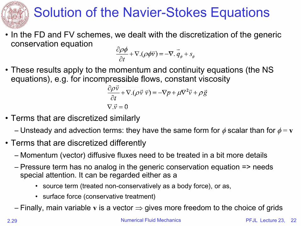
Solution of the Navier-Stokes Equations

• In the FD and FV schemes, we dealt with the discretization of the generic conservation equation

• These results apply to the momentum and continuity equations (the NS equations), e.g. for incompressible flows, constant viscosity

• Terms that are discretized similarly

– Unsteady and advection terms: they have the same form for scalar than for = v

• Terms that are discretized differently

– Momentum (vector) diffusive fluxes need to be treated in a bit more details

– Pressure term has no analog in the generic conservation equation => needs special attention. It can be regarded either as a

• source term (treated non-conservatively as a body force), or as,

• surface force (conservative treatment)

– Finally, main variable v is a vector gives more freedom to the choice of grids


.( ) .v q st

.( ) ..( ) ..( ) . .( ) . .( ) .v q s v q s.( ) .v q s.( ) . .( ) .v q s.( ) ..( ) ..( ) . .( ) ..( ) ..( ) .v q s.( ) ..( ) .v q s.( ) . .( ) .v q s.( ) ..( ) .v q s.( ) .

2.( )

. 0

v v v p v gtv

equations), e.g. for incompressible flows, constant viscosity v 2.( )v v p v g v v p v g v v p v g 2 2v v p v g v v p v g.( ) .( ).( )v v p v g.( ) .( )v v p v g.( ) 2 2 2 2v v p v g v v p v g v v p v g v v p v gv v p v g v v p v g.( )v v p v g.( ) .( )v v p v g.( ).( ) .( ) .( )v v p v g v v p v g.( )v v p v g.( ) .( )v v p v g.( )

. 0t

. 0 . 0. 0v. 0 . 0v. 0

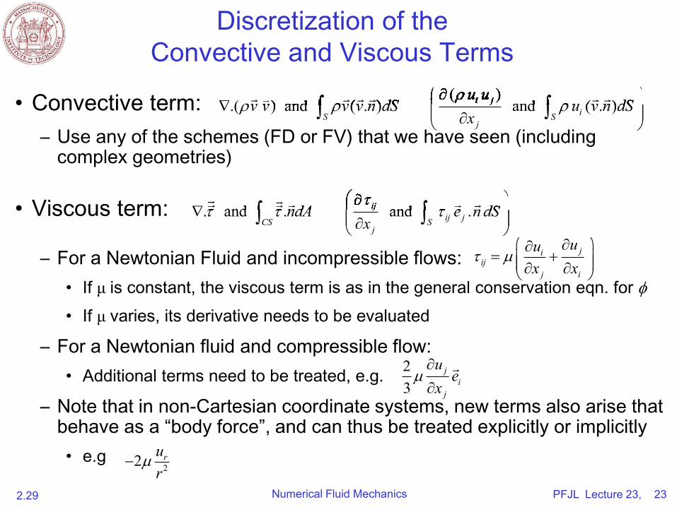
Discretization of the

Convective and Viscous Terms

• Convective term:

– Use any of the schemes (FD or FV) that we have seen (including complex geometries)

• Viscous term:

– For a Newtonian Fluid and incompressible flows:

• If μ is constant, the viscous term is as in the general conservation eqn. for

• If μ varies, its derivative needs to be evaluated

– For a Newtonian fluid and compressible flow:

• Additional terms need to be treated, e.g.

– Note that in non-Cartesian coordinate systems, new terms also arise that behave as a “body force”, and can thus be treated explicitly or implicitly

• e.g


( ).( ) and ( . ) and ( . )i j

iS Sj

u uv v v v n dS u v n dS

x

Convective term: Convective term: v v v v n dSConvective term: Convective term: .( ) and ( . )Convective term: v v v v n dSConvective term: .( ) and ( . )Convective term:

( ) ( )( )u u( ) ( )u u( )( )( ) ( )( ) and ( . ) and ( . )u v n dS u v n dS and ( . )u v n dS and ( . ) and ( . )u v n dS and ( . ) and ( . ) and ( . ) and ( . ) and ( . )

Convective term: Convective term: Convective term: v v v v n dSConvective term: Convective term: v v v v n dSConvective term: Convective term: .( ) and ( . )Convective term: v v v v n dSConvective term: .( ) and ( . )Convective term: Convective term: .( ) and ( . )Convective term: v v v v n dSConvective term: .( ) and ( . )Convective term: Convective term: .( ) and ( . )Convective term: v v v v n dSConvective term: .( ) and ( . )Convective term: Convective term: .( ) and ( . )Convective term: v v v v n dSConvective term: .( ) and ( . )Convective term: Convective term: .( ) and ( . )Convective term: v v v v n dSConvective term: .( ) and ( . )Convective term: Convective term: .( ) and ( . )Convective term: v v v v n dSConvective term: .( ) and ( . )Convective term:

( ) ( )

( ) ( )( )i j( ) ( )i j( )

( )i j( ) ( )i j( )( )u u( ) ( )u u( )

( )u u( ) ( )u u( )( )i j( )u u( )i j( ) ( )i j( )u u( )i j( )

( )i j( )u u( )i j( ) ( )i j( )u u( )i j( )( )( ) ( )( )

( )( ) ( )( )

( )

( )

( )

( ) and ( . ) and ( . ) and ( . ) and ( . )i j

i j

i j

i j( )i j( )

( )i j( )

( )i j( )

( )i j( )

( )( )

( )( )

( )( )

( )( )

( ) ( )

( ) ( )

( ) ( )

( ) ( )( )i j( ) ( )i j( )

( )i j( ) ( )i j( )

( )i j( ) ( )i j( )

( )i j( ) ( )i j( )( )u u( ) ( )u u( )

( )u u( ) ( )u u( )

( )u u( ) ( )u u( )

( )u u( ) ( )u u( )( )i j( )u u( )i j( ) ( )i j( )u u( )i j( )

( )i j( )u u( )i j( ) ( )i j( )u u( )i j( )

( )i j( )u u( )i j( ) ( )i j( )u u( )i j( )

( )i j( )u u( )i j( ) ( )i j( )u u( )i j( )( )( ) ( )( )

( )( ) ( )( )

( )( ) ( )( )

( )( ) ( )( )

Convective term: .( ) and ( . )Convective term: v v v v n dSConvective term: .( ) and ( . )Convective term: Convective term: .( ) and ( . )Convective term: v v v v n dSConvective term: .( ) and ( . )Convective term: Convective term: .( ) and ( . )Convective term: v v v v n dSConvective term: .( ) and ( . )Convective term: Convective term: Convective term: v v v v n dSConvective term: Convective term: .( ) and ( . )Convective term: v v v v n dSConvective term: .( ) and ( . )Convective term: Convective term: Convective term: Convective term: v v v v n dSConvective term: Convective term: v v v v n dSConvective term: Convective term: .( ) and ( . )Convective term: v v v v n dSConvective term: .( ) and ( . )Convective term: Convective term: .( ) and ( . )Convective term: v v v v n dSConvective term: .( ) and ( . )Convective term:

. and . and .ijij jCS S

j

ndA e n dSx

and . and .e n dS e n dS and .e n dS and . and .e n dS and . and . and . and . and .

. and .. and . . and . . and . . and .ndA ndA. and . . and . . and . . and .

ij ij

ij ij

and . and . and . and .ij

ij

ij

ij

ij ij

ij ij

ij ij

ij ij

. and .

. and . . and .ndA ndA

jiij

j i

uux x

22 rur

23

ji

j

ue

x

e

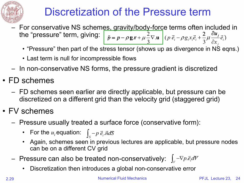
Discretization of the Pressure term

– For conservative NS schemes, gravity/body-force terms often included in the “pressure” term, giving:

• “Pressure” then part of the stress tensor (shows up as divergence in NS eqns.)

• Last term is null for incompressible flows

– In non-conservative NS forms, the pressure gradient is discretized

• FD schemes

– FD schemes seen earlier are directly applicable, but pressure can be discretized on a different grid than the velocity grid (staggered grid)

• FV schemes

– Pressure usually treated a surface force (conservative form):

• For the u equation: i

• Again, schemes seen in previous lectures are applicable, but pressure nodes can be on a different CV grid

– Pressure can also be treated non-conservatively:

• Discretization then introduces a global non-conservative error


2 2. . ( )3 3

ji i i i i

j

up p p e g x e e

x

g r u2 2 )ju

p e g x e ejp e g x e ej p e g x e e p e g x e e

2 2

2 2p e g x e e p e g x e e p e g x e e p e g x e e p e g x e e p e g x e ep p p p p p g r u g r u g r u

.iSp e ndS p e ndS

. iVp e dV p e dV


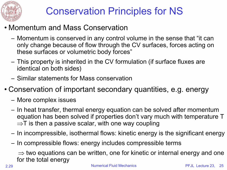
Conservation Principles for NS

• Momentum and Mass Conservation

– Momentum is conserved in any control volume in the sense that “it can only change because of flow through the CV surfaces, forces acting on these surfaces or volumetric body forces”

– This property is inherited in the CV formulation (if surface fluxes are identical on both sides)

– Similar statements for Mass conservation

• Conservation of important secondary quantities, e.g. energy

– More complex issues

– In heat transfer, thermal energy equation can be solved after momentum equation has been solved if properties don’t vary much with temperature T T is then a passive scalar, with one way coupling

– In incompressible, isothermal flows: kinetic energy is the significant energy

– In compressible flows: energy includes compressible terms

two equations can be written, one for kinetic or internal energy and one for the total energy

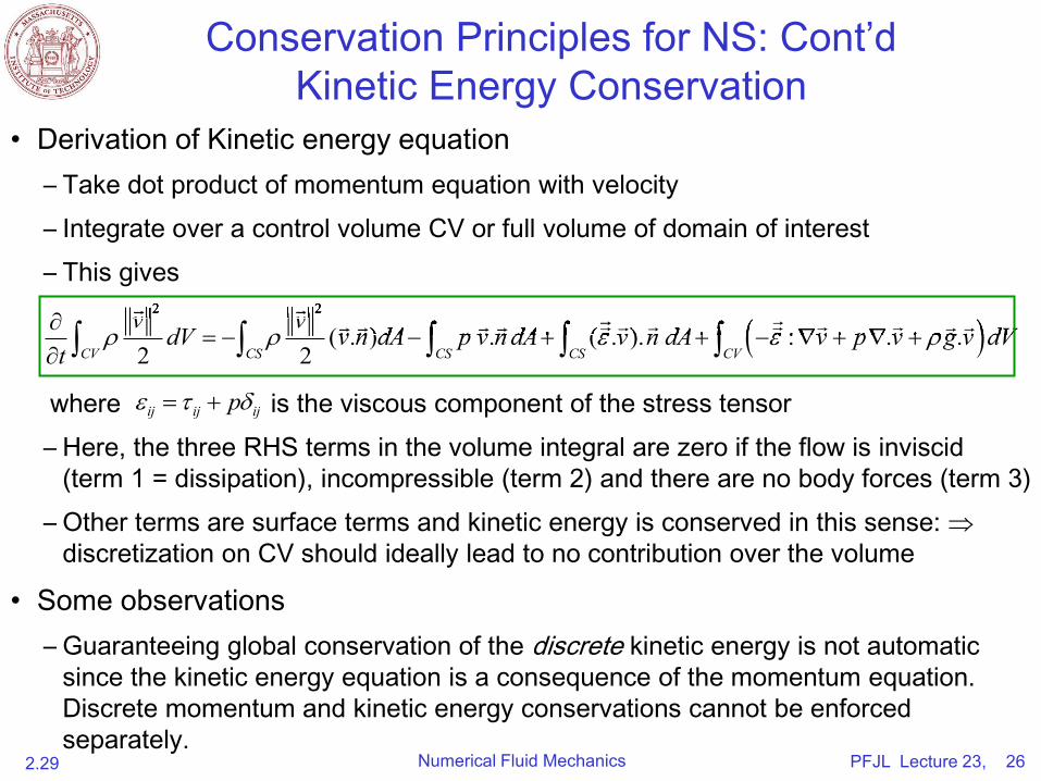
Conservation Principles for NS: Cont’dKinetic Energy Conservation

• Derivation of Kinetic energy equation

– Take dot product of momentum equation with velocity

– Integrate over a control volume CV or full volume of domain of interest

– This gives

where is the viscous component of the stress tensor

– Here, the three RHS terms in the volume integral are zero if the flow is inviscid

(term 1 = dissipation), incompressible (term 2) and there are no body forces (term 3)

– Other terms are surface terms and kinetic energy is conserved in this sense:

discretization on CV should ideally lead to no contribution over the volume

• Some observations

– Guaranteeing global conservation of the discrete kinetic energy is not automatic

since the kinetic energy equation is a consequence of the momentum equation.

Discrete momentum and kinetic energy conservations cannot be enforced

separately. 2.29 Numerical Fluid Mechanics PFJL Lecture 23, 26

2 2

( . ) . ( . ). : . .2 2CV CS CS CS CV

v vdV v n dA p v n dA v n dA v p v g v dV

t

2 22 22 22 22 2v vv vv vv vv v

v n dA p v n dA v n dA v p v g v dVv n dA p v n dA v n dA v p v g v dV: . .v n dA p v n dA v n dA v p v g v dV: . .: . .v n dA p v n dA v n dA v p v g v dV: . .: . .v n dA p v n dA v n dA v p v g v dV: . .v n dA p v n dA v n dA v p v g v dV v n dA p v n dA v n dA v p v g v dVv n dA p v n dA v n dA v p v g v dV v n dA p v n dA v n dA v p v g v dV : . .v n dA p v n dA v n dA v p v g v dV: . . : . .v n dA p v n dA v n dA v p v g v dV: . .v n dA p v n dA v n dA v p v g v dVv n dA p v n dA v n dA v p v g v dV v n dA p v n dA v n dA v p v g v dVv n dA p v n dA v n dA v p v g v dV v n dA p v n dA v n dA v p v g v dV v n dA p v n dA v n dA v p v g v dV( . ) . ( . ).v n dA p v n dA v n dA v p v g v dV( . ) . ( . ). ( . ) . ( . ).v n dA p v n dA v n dA v p v g v dV( . ) . ( . ).( . ) . ( . ).v n dA p v n dA v n dA v p v g v dV( . ) . ( . ).( . ) . ( . ).v n dA p v n dA v n dA v p v g v dV( . ) . ( . ). ( . ) . ( . ).v n dA p v n dA v n dA v p v g v dV( . ) . ( . ).( . ) . ( . ).v n dA p v n dA v n dA v p v g v dV( . ) . ( . ).( . ) . ( . ).v n dA p v n dA v n dA v p v g v dV( . ) . ( . ). ( . ) . ( . ).v n dA p v n dA v n dA v p v g v dV( . ) . ( . ). ( . ) . ( . ).v n dA p v n dA v n dA v p v g v dV( . ) . ( . ). ( . ) . ( . ).v n dA p v n dA v n dA v p v g v dV( . ) . ( . ).v n dA p v n dA v n dA v p v g v dV v n dA p v n dA v n dA v p v g v dV v n dA p v n dA v n dA v p v g v dV v n dA p v n dA v n dA v p v g v dVv n dA p v n dA v n dA v p v g v dVv n dA p v n dA v n dA v p v g v dV : . .v n dA p v n dA v n dA v p v g v dV: . .v n dA p v n dA v n dA v p v g v dV v n dA p v n dA v n dA v p v g v dVv n dA p v n dA v n dA v p v g v dV v n dA p v n dA v n dA v p v g v dV : . .v n dA p v n dA v n dA v p v g v dV: . . : . .v n dA p v n dA v n dA v p v g v dV: . .v n dA p v n dA v n dA v p v g v dVv n dA p v n dA v n dA v p v g v dV v n dA p v n dA v n dA v p v g v dVv n dA p v n dA v n dA v p v g v dVv n dA p v n dA v n dA v p v g v dV v n dA p v n dA v n dA v p v g v dV( . ) . ( . ).v n dA p v n dA v n dA v p v g v dV( . ) . ( . ). ( . ) . ( . ).v n dA p v n dA v n dA v p v g v dV( . ) . ( . ).( . ) . ( . ).v n dA p v n dA v n dA v p v g v dV( . ) . ( . ).( . ) . ( . ).v n dA p v n dA v n dA v p v g v dV( . ) . ( . ). ( . ) . ( . ).v n dA p v n dA v n dA v p v g v dV( . ) . ( . ).( . ) . ( . ).v n dA p v n dA v n dA v p v g v dV( . ) . ( . ).v n dA p v n dA v n dA v p v g v dV v n dA p v n dA v n dA v p v g v dV v n dA p v n dA v n dA v p v g v dV v n dA p v n dA v n dA v p v g v dVv n dA p v n dA v n dA v p v g v dVv n dA p v n dA v n dA v p v g v dV v n dA p v n dA v n dA v p v g v dV v n dA p v n dA v n dA v p v g v dV( . ) . ( . ).v n dA p v n dA v n dA v p v g v dV( . ) . ( . ). ( . ) . ( . ).v n dA p v n dA v n dA v p v g v dV( . ) . ( . ).

ij ij ijp

MIT OpenCourseWarehttp://ocw.mit.edu

2.29 Numerical Fluid MechanicsFall 2011

For information about citing these materials or our Terms of Use, visit: http://ocw.mit.edu/terms.

http://ocw.mit.edu

http://ocw.mit.edu/terms

Documents

2.29 Numerical Fluid Mechanics Fall 2011 Lecture 23 · 2.29 Numerical Fluid Mechanics Fall 2011 – Lecture 23 . ... – Discretization of the pressure term – Conservation principles