Finance and Economics Discussion SeriesDivisions of Research & Statistics and Monetary Affairs

Federal Reserve Board, Washington, D.C.

Bank Capital Regulations around the World: What Explains theDifferences?

Gazi Ishak Kara

2016-057

Please cite this paper as:Kara, Gazi Ishak (2016). “Bank Capital Regulations around the World: What Explains theDifferences?,” Finance and Economics Discussion Series 2016-057. Washington: Board ofGovernors of the Federal Reserve System, http://dx.doi.org/10.17016/FEDS.2016.057.

NOTE: Staff working papers in the Finance and Economics Discussion Series (FEDS) are preliminarymaterials circulated to stimulate discussion and critical comment. The analysis and conclusions set forthare those of the authors and do not indicate concurrence by other members of the research staff or theBoard of Governors. References in publications to the Finance and Economics Discussion Series (other thanacknowledgement) should be cleared with the author(s) to protect the tentative character of these papers.

Bank Capital Regulations around the World: What Explains the

Differences?∗

Gazi Ishak Kara†

First Version: May 2013This Version: July 2016

Abstract

Despite the extensive attention that the Basel capital adequacy standards have received inter-nationally, significant variation exists in the implementation of these standards across countries.Furthermore, a significant number of countries increase or decrease the stringency of capitalregulations over time. The paper investigates the empirical determinants of the variation in thedata based on the theories of bank capital regulation. The results show that countries withhigh average returns to investment and a high ratio of government ownership of banks chooseless stringent capital regulation standards. Capital regulations may also be less stringent incountries with more concentrated banking sectors.

JEL Classification Codes: G21, G28, F33

Keywords: Capital requirements, Basel capital accord, financial regulation, internationalpolicy coordination

∗I am grateful to Anusha Chari, Gary Biglaiser, Peter Norman, Richard Froyen, Sergio Parreiras, SaraswataChaudhuri, Gregory Brown, James Barth, Ross Levine, William Bassett, Vladimir Yankov and seminar participantsat the Federal Reserve Board of Governors and World Finance Conference in Venice for helpful comments andsuggestions. I thank Holt Dwyer for research assistance. All errors are mine. The analysis and the conclusions setforth are those of the author and do not indicate concurrence by other members of the research staff or the Board ofGovernors. This paper previously circulated with the title “Explaining Cross-Country and Over-Time Differences inBank Capital Regulations.”†Division of Financial Stability, Board of Governors of the Federal Reserve System, 20th Street and Constitution

Avenue N.W., Washington, D.C., 20551, E-mail: Gazi.I.Kara@frb.gov

1

1 Introduction

The first Basel capital adequacy standard signed by Group of Ten, or G-10, countries in 1988

focused on creating a level playing field for internationally active banks and improving their stability.

Somewhat unexpectedly, Basel bank capital adequacy standards received extensive attention from

all around the world, and over 100 countries voluntarily adopted Basel I (Pattison, 2006). Basel I

was updated in 2004 (popularly known as Basel II) with more sophisticated rules and principles,

and again in 2010 with enhanced capital, liquidity, and leverage requirements following the global

financial crisis (Basel III). A survey done by the Bank for International Settlements (BIS) in

2015 shows that all 27 Basel Committee on Banking Supervision (BCBS) member countries had

implemented enhanced risk-based capital regulations by the end of 2013.1 A separate survey by

the Financial Stability Institute (FSI) shows that 95 out of 117 non-Basel Committee member

jurisdictions that are monitored have adopted or are in the process of adopting Basel III as of mid-

2015.2 These interests suggest that Basel principles have become a model for capital regulation by

national banking systems in both developed and developing countries.

The adoption of Basel principles by the majority of countries around the globe is an important

fact; however, what is more important is how countries are actually implementing those principles

in practice. The Basel principles for bank regulation are rich and complex in nature, which gives

countries a substantial amount of leeway in their implementation(Concetta Chiuri et al., 2002). A

country may announce the adoption of an 8 percent minimum capital ratio (the percentage of a

bank’s capital compared with its risk-weighted assets) that is required by Basel rules. However,

the effective capital adequacy ratio will be determined by how the regulator of this country allows

domestic banks to choose the numerator (equity capital) and the denominator (risk-weighted assets)

of this ratio. For example, a regulator can loosely define the items that banks can include in their

equity capital, or the risk weights in the denominator may not reflect a bank’s market or credit risk,

contrary to the Basel recommendations. The freedom in the implementation of Basel principles

is expected to be larger, especially for the non-BCBS countries. Nevertheless, the data show a

significant variation even among the BCBS member countries.

Fortunately, a carefully executed survey series by the World Bank allows us to compare the

actual implementation of Basel bank capital regulations across over 100 countries. These surveys,

conducted four times between 1999 and 2011, reveal that the stringency of bank capital regulations

not only differs by significant amounts across countries (see figure 1), but also varies over time for

a given country (see figure 2). The aim of this paper is to investigate the empirical determinants

of this variation based on theories of capital regulation and previous empirical studies. I develop

testable hypotheses from the literature to investigate the effects of the structure of the banking

1Basel Committee on Banking Supervision, Implementation of Basel standards, November 2015, available atwww.bis.org/bcbs/publ/d345.htm.

2FSI Survey – Basel II, 2.5 and III Implementation, July 2015, available at www.bis.org/fsi/fsiop2015.htm.

2

system and the economic, political and institutional characteristics of countries on the stringency

of bank capital regulations.

Theoretical motivations for bank capital regulations are mainly focused on the role of capital

in the creation of incentives for bank owners to take socially efficient levels of risk. Moral hazard

and agency problems often cause bank owners and managers to take excessive risks. Incorrectly

priced deposit insurance, created to prevent bank runs in the first place, and limited liability are

widely blamed for distorting the risk behavior of bank owners (Kroszner, 1998; Allen and Gale,

2003). Deposit insurance and limited liability provide a safety net for bank owners by which

they reap the benefits of excessive risk taking in “good times” but do not bear the full costs in

“bad times”. Regulators expect bank owners to behave more prudently and responsibly if they have

“skin in the game”, which happens when bank owners invest their own capital in the bank. Another

justification for capital regulations is the existence of welfare-relevant pecuniary externalities (Allen

and Gale, 2003; Lorenzoni, 2008; Korinek, 2011; Kara and Ozsoy, 2016). These studies show that

in competitive markets, atomistic banks fail to internalize the effects of their portfolio choices, such

as the sizes of their risky assets and liquidity buffers, on the fire sale price of assets during times

of distress and, as a result, they take socially excessive amounts of risk. Hence, capital regulations

can be used to implement a socially efficient level of risk-taking in the banking system.

In a recent study, Kara (2016) justifies capital regulations under the existence of fire sale ex-

ternalities and shows that a country with higher returns on investment chooses a lower minimum

regulatory capital ratio than a low-return country. In his model, less stringent capital regulations

allow banks to invest more in risky assets and hence take a larger exposure to fire sale risk. Higher

average returns on investment reduce both the social and private marginal cost of the fire sale

risk and, as a result, regulators relax capital requirements. I test this hypothesis and show that

a negative relationship exists between returns on investment and the stringency of bank capital

regulations.

Dell’Ariccia and Marquez (2006) use limited liability and the existence of deposit insurance to

justify capital regulations and show that regulators who are more concerned about the profits of

the banking sector than about financial stability choose less stringent capital regulations. They

consider a two-country model with a single bank in each country. Regulators of the two countries

compete by setting the minimum capital ratios. Regulators choose capital ratios to maximize

expected domestic social welfare, which is a weighted average of bank profits and a measure of

financial stability. Regulators can differ in terms of the weight that they attach to bank profits

in their objective functions. This weight reflects the degree to which regulators are captured by

the financial institutions under their control. The authors show that the country with a higher

regulatory capture chooses a less stringent capital requirement. The results in this paper paper

confirm this hypothesis.

Additionally, I test whether the stringency of capital regulations is significantly related to

3

the competitiveness of the banking sector. Because one main theoretical justification for capital

requirements is to limit excessive risk-taking by banks, one would expect regulators to respond to

measures that affect how much risk banks are willing to take.3 The competitiveness of the banking

sector has been considered one of the main determinants of the risk-taking incentives of banks

(Allen and Gale, 2004).

There are two contradictory views on the relationship between concentration and financial sta-

bility. The conventional view, which is also called the “concentration-stability” hypothesis by Berger

et al. (2004), posits that more concentrated financial sectors with a few large banks are more stable.

On the opposite side, the “concentration-fragility” view asserts that there is a negative relationship

between concentration and financial stability: An increase in concentration reduces the stability of

the banking sector. If regulators respond to higher concentration by tightening capital regulations

they must be perceiving higher risks in the sector as a result of higher concentration. Therefore,

in the regressions, a positive relationship between the stringency of bank capital regulations and

concentration ratio will support the concentration-fragility hypothesis, and a negative relationship

between the two will support the concentration-stability hypothesis. In this paper, I obtain some

evidence for a negative relationship between concentration ratio and the stringency of bank capital

regulations; hence, my results favor the concentration-stability hypothesis.

Furthermore, the theory points out that the experience of a recent financial crisis is a driving

force for more stringent capital regulations. Aizenman (2009) considers a dynamic model in which

agents are subject to idiosyncratic uncertainty regarding their exposure to financial crisis incidence.

The agents, at each point in time, update their perceived probability of a financial crisis in the next

period in a Bayesian manner. Aizenman shows that a longer spell of “good times,” a run with no

financial crises, reduces the perceived mean of a crisis in the next period, which in turn reduces the

regulation intensity. In addition to the channel suggested by Aizenman, the incidence of financial

crisis generates social and political capital for bank regulators to enact more stringent prudential

reforms. The recent global financial crisis provides a good real-world example, as it paved the

way for stronger bank regulations all around the world, such as the introduction of Basel III rules

in 2010 and, in the United States, the implementation of enhanced financial regulations under the

2010 Dodd-Frank Wall Street Reform and Consumer Protection Act. Therefore, I also test whether

there is a negative relationship between the time since the most recent systemic banking crisis a

country has experienced and the intensity of bank capital regulations. However, I do not find any

evidence to support this hypothesis.

In the regressions, I also control for the depth, size and efficiency of financial markets, but I do

not find statistically significant effects of these variables on the stringency of capital regulations.

I find some evidence that capital regulations are less stringent in countries where the deposit

insurer has more power. Additionally, I control for the political structure and institutional quality

3Both theoretical and empirical literature produce mixed predictions on the effectiveness of capital regulations inlimiting the risk-taking behavior of banks. See VanHoose (2007) for an extensive survey of this literature.

4

of countries and find that countries with competitive and democratic political systems choose

more stringent capital regulations. However, I do not find any statistically significant effect of the

independence of the legal system and the quality of institutions that protect property rights on the

stringency of capital regulations.

The paper proceeds as follows. Section 2 provides a brief review of the related literature. Section

3 describes the data and provides descriptive statistics for the dependent and independent variables.

Section 4 explains the econometric methodology and presents the results for the benchmark model.

Section 5 contains the robustness checks, including the estimation of a dynamic model. Section 6

concludes. The appendix contains the figures and tables.

2 Literature review

This paper is part of the broader literature that investigates the determinants of bank regulations

in general. To the best of my knowledge, this paper is the first to investigate the empirical de-

terminants of cross-country and over-time variation in the stringency of bank capital regulations

in particular. Barth et al. (2006) assess whether cross-country differences in political institutions

explain national choices of supervisory and regulatory policies. They use cross-sectional data from

the 1999 World Bank survey of bank regulations (one of the four surveys that is used in this study)

and show that the organization and operation of political systems shape bank supervisory and

regulatory practices.

This study is different from Barth et al. (2006) in several ways. First, the aim of this study

is to explain the cross-country and over-time variation in the stringency of capital regulations

in particular, whereas Barth et al. (2006) focus on the cross-country variation in broader bank

supervisory and regulatory practices, such as bank activity restrictions, the strength of private

monitoring, and the power of banking supervisors. Second, the focus of this study is to explain the

variation seen in the data based on the economic and financial structure of countries, while Barth

et al. (2006) are mainly interested in investigating the institutional and political determinants of

bank regulations. In this study, I explicitly or implicitly control for such political and institutional

characteristics of countries. Third, unlike Barth et al. (2006), I employ a panel data set that allows

me to explain not only the cross-country differences in capital regulations but also the change that

occurs over time in these regulations.

A separate literature examines the variation in actual bank capital ratios but not the overall

stringency of bank capital regulations. An important part of this literature discusses whether

capital ratios in practice are pro-cyclical or counter-cyclical. Some studies focus on bank data

from a single country, while others use bank data from several countries. Notable studies in this

literature include Bikker and Metzemakers (2004), Ayuso et al. (2004), and Andersen (2011).

In a related study, Brewer et al. (2008) investigate the cross-country differences in the actual

bank capital ratios of internationally active banks in 12 developed nations. Their explanatory

5

variables include bank-specific factors such as bank size, country-specific macroeconomic factors

such as real GDP growth rate, country-specific public and regulatory policy factors, and control

variables such as differences in accounting standards. This study differs from Brewer et al. (2008)

mainly in its interest in explaining the regulatory choices of bank capital regulations, not the actual

capital ratios of individual banks. Furthermore, their study includes only 12 developed countries,

whereas I investigate the determinants of capital regulations using a sample of 21 developed and

45 developing economies.

3 Data and descriptive statistics

This study employs an unbalanced panel data set. The measure used for the stringency of bank

capital regulations is the “Overall Capital Stringency” index created by James R. Barth, Gerard

Caprio, and Ross Levine, which is based on extensive World Bank surveys on bank regulations

initiated by these authors in the late 1990s. These surveys were conducted four times and represent

the situation of bank regulations around the world at the ends of 1999, 2002, 2006, and 2011.4 The

last survey includes around 300 questions, and 180 countries responded to at least one of the four

surveys.

This study restricts attention to a smaller set of countries. My sample consists of 66 major

countries that are also included in a recent study by Gourinchas and Obstfeld (2012). This smaller

sample does not include low-income countries or very small countries, some of which are known as

offshore financial centers, such as the British Virgin Islands or Mauritius. Using the classification

in Gourinchas and Obstfeld (2012), there are 21 advanced and 45 emerging countries in our sample.

Table 4 lists the names of the countries in each group according to the income categories defined

by the World Bank (high income, upper-middle income, and middle income). All 21 advanced

economies are in the high per capita income group. Of the 45 developing countries, 11 are in

the high-income group, 25 are in the upper-middle-income group, and 9 are in the middle-income

group.

World Bank regulation surveys were carefully executed. Surveys were sent to senior officers

in the main regulatory agency of each country, and whenever there were conflicting or confusing

answers to questions, the authors double-checked the information by both contacting regulators in

the corresponding country and referring to other sources, including the information collected by the

U.S. Office of the Comptroller of the Currency (OCC) and the Institute of International Bankers

(Barth et al., 2004).

Barth et al. (2004) define the “Overall Capital Stringency” index as a measure of “whether

the capital requirement reflects certain risk elements and deducts certain market value losses from

capital before minimum capital adequacy is determined”. The index was originally based on the

4I use the recently compiled panel data from responses to all four surveys by the same authors. See Barth et al.(2013) for an extensive discussion of this panel data set.

6

responses to seven questions in the Capital Regulatory Variable section of the surveys. In this

study, I create the index using six of the seven questions, which are given in table 1.5 A value

of 1 is assigned to each “yes” answer, and a value of 0 is assigned to each “no” answer. The

index therefore takes values between 0 and 6, and higher values of the index correspond to greater

stringency of bank capital regulations.

The six questions used in the creation of the index are derived from Basel bank capital adequacy

principles. The Basel capital adequacy ratio is equal to the equity capital divided by risk-weighted

assets. The questions in Table 1 can be considered in two broad groups. The first group of

questions (3.1.1, 3.2, and 3.3) measure a country’s compliance with Basel risk guidelines, and the

second group concern the calculation of capital. In other words, the first group of questions concern

the determination of the weights in the denominator of the capital ratio, whereas the second group

deal with the determination of capital in the numerator of this ratio. Therefore, this index gives

us a measure of the stringency of bank capital regulations that is comparable across countries and

over time.

Table 1: Capital stringency index questions

3.1.1 Is the minimum capital ratio risk weighted in line with the Basel guidelines? Yes/No3.2 Does the minimum ratio vary as a function of an individual bank’s credit risk? Yes/No3.3 Does the minimum ratio vary as a function of market risk? Yes/No3.9 Before minimum capital adequacy is determined, which of the following are deductedfrom the book value of capital?

3.9.1 Market value of loan losses not realized in accounting books? Yes/No3.9.2 Unrealized losses in securities portfolios? Yes/No3.9.3 Unrealized foreign exchange losses? Yes/No

Figure 1 shows the distribution of overall capital stringency indexes for each survey. The figure

reveals that there is a significant variation in the stringency of bank capital regulations across

countries for each of the four survey years. The mean of the index for each survey year is 3.4, 3.60,

3.39, and 5.11, respectively, with standard deviations of 1.66, 1.56, 1.75 and 1.40. The percentage

of countries with an index value that is below the mean is 50 percent in 1999, 42 percent in 2002, 57

percent in 2006, and 28 percent in 2011. The average capital stringency index rises by a significant

amount after the global financial crisis, and its standard deviation shrinks; however, the cross-

country variation does not disappear. Figure 1 shows that after the global financial crisis, the

distribution becomes significantly skewed to the right, indicating that there is an overall increase

in the stringency of capital regulations around the world.

5I exclude the following question from the calculation of the index: “What fraction of revaluation gains is allowedas part of capital?”. First, answers to this question are not as objective as the answers to the other six questions,and hence, quantification of those answers poses a serious challenge. Second, including this question severely reducesthe data availability.

7

Figure 2 shows that there is also a significant variation in the stringency of bank capital reg-

ulations over time. Each panel shows the distribution of the change in the capital stringency

index for individual countries compared with the previous survey (that is, the distribution of

capital stringencyit−capital stringencyi,t−1). Strikingly, the direction of the change in capital regu-

lations is not positive for all countries over time. Among 47 countries in the sample that responded

to both 2002 and 1999 surveys, 7 countries (15 percent) reduced the stringency of capital regu-

lations compared with the previous survey, whereas 26 countries (55 percent) kept the regulation

level the same, and 14 countries (30 percent) strengthened their regulations. A larger percentage

of countries relaxed their regulatory standards between 2002 and 2006: Among 49 countries in the

sample that responded to both 2002 and 2006 surveys, 15 countries (30 percent) relaxed the strin-

gency of capital regulations compared with the previous survey, whereas 16 countries (33 percent)

kept the regulation level the same and 18 countries (37 percent) strengthened their regulations.

The distribution changes significantly after the recent financial crisis and becomes right-skewed.

Among 51 countries in the sample that responded to the last two surveys, only 6 of them (11 per-

cent) reduced the stringency of capital regulations; 12 countries (25 percent) kept the regulation at

the same level, and 33 countries (64 percent) increased the stringency of bank capital regulations.

Which components drive the changes in the capital stringency index from one survey year to

another? Looking at the changes in the components of the aggregate index, presented in figure 3,

reveals that there is almost no variation in the number of countries that follow the Basel guidelines

for capital ratio risk weights from one survey to another: Almost all countries in our sample claim

that they follow these guidelines in all four surveys. Hence, the variations in the aggregate index

over time are determined by the remaining five components. In 2002, an overwhelming majority (70

to 80 percent) of the countries kept individual components unchanged relative to the 1999 survey.

Furthermore, the number of countries that relaxed each component was roughly equal to the number

of countries that tightened it. The only exception was the component on the deduction of unrealized

losses in security portfolios from the book value of capital (question 3.9.2 in table 1). About 20

percent of countries enacted this component, whereas only 9 percent stopped implementing it.

In 2006, the percentages of countries that kept individual components unchanged remained

high despite decreasing somewhat compared with the previous survey. Additionally, more countries

implemented components related to credit risk and market risk than disregarded such rules, whereas

the opposite was true for components related to the determination of equity capital (questions 3.9.1,

3.9.2, and 3.9.3 in table 1). Apparently, the overall tendency toward relaxing the capital regulation

stringency in 2006 was driven mainly by changes in these components.

Finally, in 2011, the general increase in the stringency of capital regulations were mainly driven

by the components related to incorporating credit risk and market risk into capital risk weights. In

particular, no countries disregarded implementing these two components. In fact, a larger number

of countries enacted these rules than kept their current rulings. Meanwhile, a significant number

8

of countries (15 to 20 percent) abandoned deducting unrealized losses in loan values, security

portfolios, and foreign exchange holdings. Nevertheless, the numbers of countries that started to

implement these components were larger (22 to 41 percent), and even more countries kept these

components unchanged compared with the previous survey (47 to 61 percent).

3.1 Discussion of variables

In this section, I introduce the explanatory variables to test the hypothesis developed in the intro-

duction based on the theories of bank capital regulations. Table 2 provides the variable definitions

along with data sources, and table 3 provides summary statistics for the dependent and independent

variables.

To test the relationship between returns on investment and the intensity of bank capital reg-

ulations, stock market returns or real GDP growth rate can be used as a proxy for the average

returns on investment. I choose the latter for several reasons. First, GDP growth rate is a good

proxy for average returns on various types of investments in an economy and is the most important

economic benchmark that policymakers base decisions upon. Second, there are many undercapi-

talized developing countries in our sample, and GDP growth rate is more representative of overall

average returns than stock market gains for this group. Lastly, GDP growth rate data are more

easily available for a large number of countries and much less volatile than stock market returns.6 I

obtain the expected GDP growth rate from the Consensus Economic Forecast database. Expected

GDP growth is the average of the surveyed forecasters’ next-year GDP growth expectations for

each country as of November or December of the survey year, based on data availability.

Even if two countries have the same asset returns, differences in the risk profile of these returns

could potentially lead to a divergence in regulatory choices. To control for the risk profile of a

country, I employ the Political Risk Services (PRS) country economic risk indicator.7 This is a

monthly indicator that ranges from a high of 50 (least risk) to a low of 0 (highest risk), though in

practice the lowest ratings are generally near 15.8 Table 3 shows that within the sample, the index

varies between 24 and 47.5. In addition, I use the standard deviation of a 10-year rolling window

of the standard deviation of real GDP growth rate as a measure of the economic risk of a country

and obtain qualitatively similar results.9

I use the government-owned banks variable to test the relationship between regulatory capture

and the stringency of capital regulations. Government-owned banks is the percentage of a banking

system’s assets in banks that are 50 percent or more owned by the government. These data are

also obtained from the World Bank regulation surveys. Table 3 shows that the ratio of government

6I performed a robustness check using available stock market return data, and the qualitative results did notchange.

7“Country Data Online.” The PRS Group. http://epub.prsgroup.com/the-countrydata-gateway.8I use the five-year average of the index to focus on medium to long-term economic risks for each country.9These results are not presented here but available upon request from the author.

9

ownership of banks takes values between 0 and 80 percent in our sample, with mean 17 percent

and standard deviation 20. This ratio varies significantly across countries but it fluctuates less over

time for a given country. Advanced countries had very low or no government ownership in the

banking sector before the recent crisis.10 The last survey reveals that this ratio is increasing for

some advanced economies (Austria, Switzerland, United Kingdom, Ireland and the Netherlands)

in the aftermath of the global recession in large part because of nationalizations and crisis-related

capital injections.

I use the fraction of government-owned banks as a proxy for regulatory capture. If a country

has a high ratio of government-owned banks, then one would expect the regulator of that country

to be more concerned about banking-sector profits as opposed to financial stability and hence to

choose less stringent regulations, as suggested by Dell’Ariccia and Marquez (2006). Therefore,

I test whether there is a negative relationship between the stringency of capital regulations and

government-owned banks.

In a similar vein, I also control for the involvement of the government in the overall economy

of a country, as a government’s involvement in the economy may influence its preferences toward

bank regulation. This variable is taken from the Economic Freedom of the World database and is

the average of four variables that measure different aspects of a government’s involvement in the

economy. The summary “government size” index takes values between 0 and 10, and higher values

indicate a larger government role. The components of the index are government consumption as

a percentage of total consumption; general government transfers and subsidies as a percentage

of GDP; an index on the number, composition, and share of output supplied by state-operated

enterprises and government investment as a share of total investment; and an index of the top

marginal tax rate.11 Government size is correlated with the variables that measure political and

institutional characteristics of countries and hence can be considered a control variable in that

regard, as well. In fact, in section 5.3, I replace the government size variable with specific variables

that control for the political structure or institutional quality, and the results do not change.

To test the relationship between bank capital regulations and the competitiveness of the banking

sector, I use the three-bank concentration ratio. This variable is obtained from the Financial

Development and Structure Database (Beck et al., 2009; Cihak et al., 2012). The variable is the

ratio of the assets of a country’s three largest banks to the assets of all commercial banks in that

country. The authors calculate this ratio from Bureau van Dijk’s BankScope database.12 Table

3 shows that the concentration ratio varies between 15.28 and 100 percent, with mean 57 percent

and standard deviation 19.13 The intensity of competition in the banking sector, which is usually

10Germany, Portugal, Greece, and Switzerland are exceptions in that regard with 40 percent, 25 percent, 23 percent,and 11.5 percent government-owned bank ratios, respectively, according to the last figures before the crisis.

11I use the three-year averages of this variable to smooth out potential short-term volatility government expendi-tures.

12Bankscope. Bureau van Dijk. https://bankscope.bvdinfo.com/13Similarly to the government size variable, I use the three-year averages of this variable as well to smooth out

10

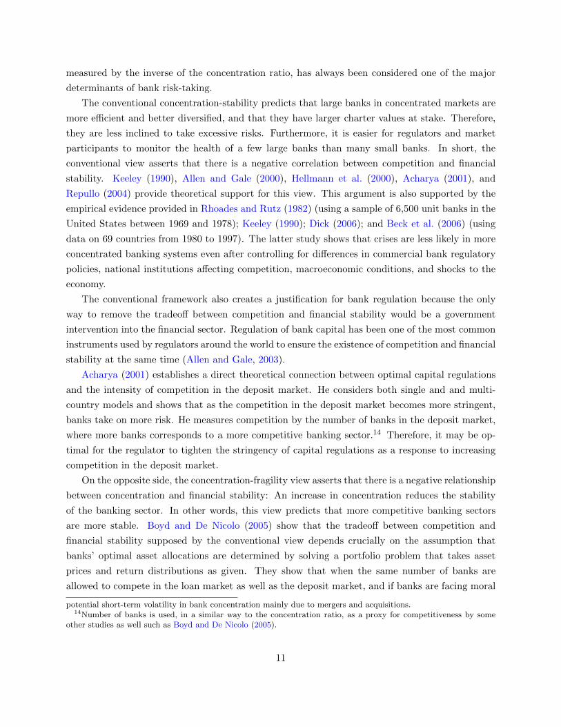
measured by the inverse of the concentration ratio, has always been considered one of the major

determinants of bank risk-taking.

The conventional concentration-stability predicts that large banks in concentrated markets are

more efficient and better diversified, and that they have larger charter values at stake. Therefore,

they are less inclined to take excessive risks. Furthermore, it is easier for regulators and market

participants to monitor the health of a few large banks than many small banks. In short, the

conventional view asserts that there is a negative correlation between competition and financial

stability. Keeley (1990), Allen and Gale (2000), Hellmann et al. (2000), Acharya (2001), and

Repullo (2004) provide theoretical support for this view. This argument is also supported by the

empirical evidence provided in Rhoades and Rutz (1982) (using a sample of 6,500 unit banks in the

United States between 1969 and 1978); Keeley (1990); Dick (2006); and Beck et al. (2006) (using

data on 69 countries from 1980 to 1997). The latter study shows that crises are less likely in more

concentrated banking systems even after controlling for differences in commercial bank regulatory

policies, national institutions affecting competition, macroeconomic conditions, and shocks to the

economy.

The conventional framework also creates a justification for bank regulation because the only

way to remove the tradeoff between competition and financial stability would be a government

intervention into the financial sector. Regulation of bank capital has been one of the most common

instruments used by regulators around the world to ensure the existence of competition and financial

stability at the same time (Allen and Gale, 2003).

Acharya (2001) establishes a direct theoretical connection between optimal capital regulations

and the intensity of competition in the deposit market. He considers both single and and multi-

country models and shows that as the competition in the deposit market becomes more stringent,

banks take on more risk. He measures competition by the number of banks in the deposit market,

where more banks corresponds to a more competitive banking sector.14 Therefore, it may be op-

timal for the regulator to tighten the stringency of capital regulations as a response to increasing

competition in the deposit market.

On the opposite side, the concentration-fragility view asserts that there is a negative relationship

between concentration and financial stability: An increase in concentration reduces the stability

of the banking sector. In other words, this view predicts that more competitive banking sectors

are more stable. Boyd and De Nicolo (2005) show that the tradeoff between competition and

financial stability supposed by the conventional view depends crucially on the assumption that

banks’ optimal asset allocations are determined by solving a portfolio problem that takes asset

prices and return distributions as given. They show that when the same number of banks are

allowed to compete in the loan market as well as the deposit market, and if banks are facing moral

potential short-term volatility in bank concentration mainly due to mergers and acquisitions.14Number of banks is used, in a similar way to the concentration ratio, as a proxy for competitiveness by some

other studies as well such as Boyd and De Nicolo (2005).

11

hazard from borrowers in the loan market, then the banking sector becomes less risky as it gets

more competitive. They measure competitiveness by the number of banks. Proponents of this view

also argue that the existence of a few large banks generates an implicit “too-big-to-fail” guarantee

and creates incentives for banks to take excessive risks. Jayaratne and Strahan (1998), using U.S.

bank data from between 1975 and 1992; De Nicolo (2000); De Nicolo et al. (2004); Boyd et al.

(2006); De Nicolo and Loukoianova (2007); and Schaeck et al. (2009) provide empirical support for

the concentration-fragility view.

In addition to studies that take a particular view in this discussion, some studies argue that the

relationship between competition and financial stability is too complex to take a particular position.

Allen and Gale (2004) consider a series of models and show that different models provide different

predictions. The models considered include general equilibrium models of financial intermediaries

and markets, agency models, and models of spatial competition, Schumpeterian competition, and

contagion. Their analysis suggests that general equilibrium and Schumpeterian competition models

require the coexistence of competition and financial stability for efficiency, as opposed to the tradeoff

between those two that is conventionally supposed.

To summarize, the theoretical and empirical evidence with respect to the relationship between

concentration ratio and the riskiness of the banking sector is mixed: A higher concentration ratio

may increase or decrease banks’ incentive to take excessive risks. A priori, my study does not take a

particular side on this theoretical and empirical divide. If regulators respond to higher concentration

in the banking sector by relaxing capital regulations, they must be perceiving lower risks in the

sector as a result of higher concentration. Hence, a negative relationship between the stringency

of bank capital regulations and concentration ratio in our regressions will support the conventional

concentration-stability hypothesis. Similarly, a positive relationship between the stringency of bank

capital regulations and concentration ratio will support the concentration-fragility hypothesis.

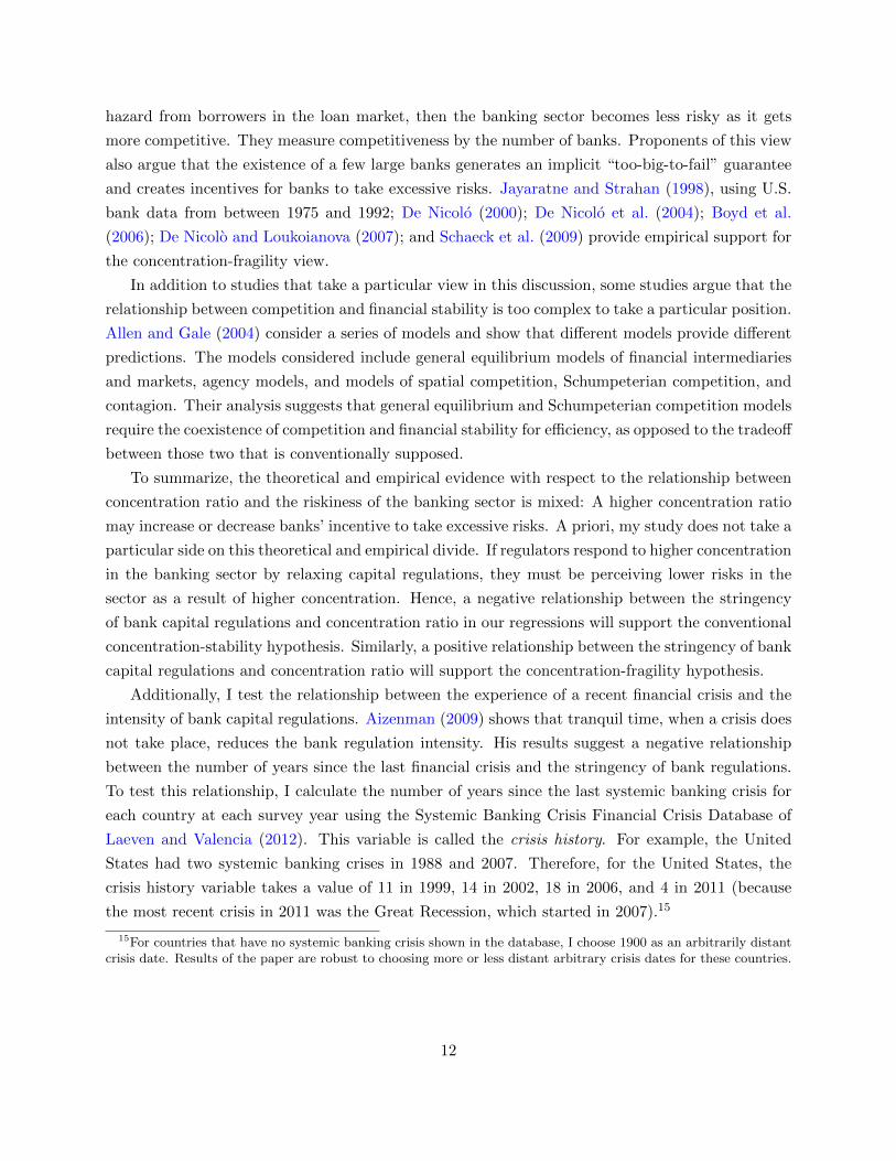
Additionally, I test the relationship between the experience of a recent financial crisis and the

intensity of bank capital regulations. Aizenman (2009) shows that tranquil time, when a crisis does

not take place, reduces the bank regulation intensity. His results suggest a negative relationship

between the number of years since the last financial crisis and the stringency of bank regulations.

To test this relationship, I calculate the number of years since the last systemic banking crisis for

each country at each survey year using the Systemic Banking Crisis Financial Crisis Database of

Laeven and Valencia (2012). This variable is called the crisis history. For example, the United

States had two systemic banking crises in 1988 and 2007. Therefore, for the United States, the

crisis history variable takes a value of 11 in 1999, 14 in 2002, 18 in 2006, and 4 in 2011 (because

the most recent crisis in 2011 was the Great Recession, which started in 2007).15

15For countries that have no systemic banking crisis shown in the database, I choose 1900 as an arbitrarily distantcrisis date. Results of the paper are robust to choosing more or less distant arbitrary crisis dates for these countries.

12

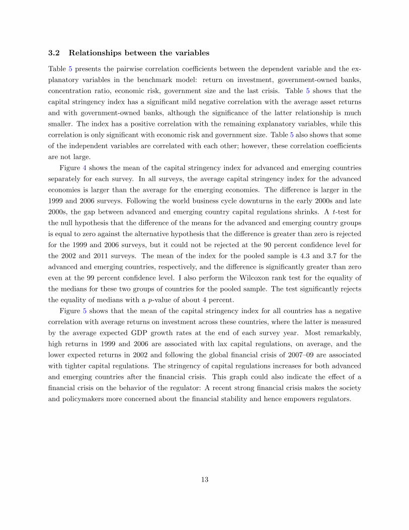
3.2 Relationships between the variables

Table 5 presents the pairwise correlation coefficients between the dependent variable and the ex-

planatory variables in the benchmark model: return on investment, government-owned banks,

concentration ratio, economic risk, government size and the last crisis. Table 5 shows that the

capital stringency index has a significant mild negative correlation with the average asset returns

and with government-owned banks, although the significance of the latter relationship is much

smaller. The index has a positive correlation with the remaining explanatory variables, while this

correlation is only significant with economic risk and government size. Table 5 also shows that some

of the independent variables are correlated with each other; however, these correlation coefficients

are not large.

Figure 4 shows the mean of the capital stringency index for advanced and emerging countries

separately for each survey. In all surveys, the average capital stringency index for the advanced

economies is larger than the average for the emerging economies. The difference is larger in the

1999 and 2006 surveys. Following the world business cycle downturns in the early 2000s and late

2000s, the gap between advanced and emerging country capital regulations shrinks. A t-test for

the null hypothesis that the difference of the means for the advanced and emerging country groups

is equal to zero against the alternative hypothesis that the difference is greater than zero is rejected

for the 1999 and 2006 surveys, but it could not be rejected at the 90 percent confidence level for

the 2002 and 2011 surveys. The mean of the index for the pooled sample is 4.3 and 3.7 for the

advanced and emerging countries, respectively, and the difference is significantly greater than zero

even at the 99 percent confidence level. I also perform the Wilcoxon rank test for the equality of

the medians for these two groups of countries for the pooled sample. The test significantly rejects

the equality of medians with a p-value of about 4 percent.

Figure 5 shows that the mean of the capital stringency index for all countries has a negative

correlation with average returns on investment across these countries, where the latter is measured

by the average expected GDP growth rates at the end of each survey year. Most remarkably,

high returns in 1999 and 2006 are associated with lax capital regulations, on average, and the

lower expected returns in 2002 and following the global financial crisis of 2007–09 are associated

with tighter capital regulations. The stringency of capital regulations increases for both advanced

and emerging countries after the financial crisis. This graph could also indicate the effect of a

financial crisis on the behavior of the regulator: A recent strong financial crisis makes the society

and policymakers more concerned about the financial stability and hence empowers regulators.

13

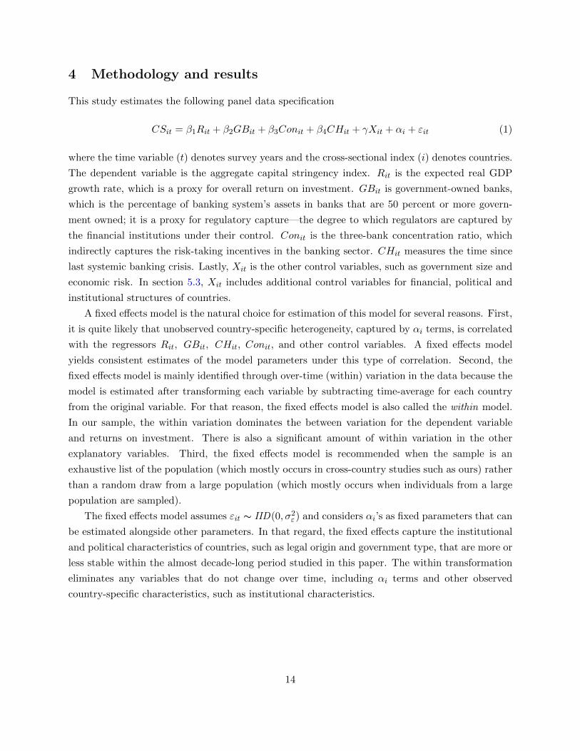
4 Methodology and results

This study estimates the following panel data specification

CSit = β1Rit + β2GBit + β3Conit + β4CHit + γXit + αi + εit (1)

where the time variable (t) denotes survey years and the cross-sectional index (i) denotes countries.

The dependent variable is the aggregate capital stringency index. Rit is the expected real GDP

growth rate, which is a proxy for overall return on investment. GBit is government-owned banks,

which is the percentage of banking system’s assets in banks that are 50 percent or more govern-

ment owned; it is a proxy for regulatory capture—the degree to which regulators are captured by

the financial institutions under their control. Conit is the three-bank concentration ratio, which

indirectly captures the risk-taking incentives in the banking sector. CHit measures the time since

last systemic banking crisis. Lastly, Xit is the other control variables, such as government size and

economic risk. In section 5.3, Xit includes additional control variables for financial, political and

institutional structures of countries.

A fixed effects model is the natural choice for estimation of this model for several reasons. First,

it is quite likely that unobserved country-specific heterogeneity, captured by αi terms, is correlated

with the regressors Rit, GBit, CHit, Conit, and other control variables. A fixed effects model

yields consistent estimates of the model parameters under this type of correlation. Second, the

fixed effects model is mainly identified through over-time (within) variation in the data because the

model is estimated after transforming each variable by subtracting time-average for each country

from the original variable. For that reason, the fixed effects model is also called the within model.

In our sample, the within variation dominates the between variation for the dependent variable

and returns on investment. There is also a significant amount of within variation in the other

explanatory variables. Third, the fixed effects model is recommended when the sample is an

exhaustive list of the population (which mostly occurs in cross-country studies such as ours) rather

than a random draw from a large population (which mostly occurs when individuals from a large

population are sampled).

The fixed effects model assumes εit ∼ IID(0, σ2ε) and considers αi’s as fixed parameters that can

be estimated alongside other parameters. In that regard, the fixed effects capture the institutional

and political characteristics of countries, such as legal origin and government type, that are more or

less stable within the almost decade-long period studied in this paper. The within transformation

eliminates any variables that do not change over time, including αi terms and other observed

country-specific characteristics, such as institutional characteristics.

14

4.1 Results

Table 6 presents the estimation of the model given by equation (1) using the fixed effects strategy.

The benchmark fixed effects model in the first column predicts a significant and negative effect

of returns on investment, government-owned banks, and concentration ratio on the stringency of

bank capital regulations. The remaining three explanatory variables (economic risk, government

size, and crisis history) do not have any significant effects on the stringency of capital regulations.

The particularly strong negative coefficient on the return on investment variable indicates that

high return countries choose less stringent bank capital regulation. This result could be explained

if higher returns allow a country to take on more risk through less stringent regulations because

lax capital regulations translate into larger losses from bank defaults and fire sales during distress

times, as in Kara (2016).

Estimation of the fixed effects model shows that a 1 percentage point increase in the average

rate of return on investment reduces the stringency of the capital regulation index by 0.4 point.

This coefficient is not only statistically highly significant, but it is also economically strong. The

following exercise helps us to see the economic significance of the coefficient: What change in the

GDP growth rate would be necessary for an emerging country to have the capital stringency level

of an advanced country? The mean of the index is 4.3 for the advanced countries and 3.7 for the

emerging countries. Because the difference between the two means is equal to 0.6, the coefficient

on the return variable implies that, holding everything else constant, if emerging countries had

lower return rates, by 1.5 percentage points, on average, they would choose the same level of bank

capital stringency as the developed countries (0.6/0.4 = 1.5). This number is reasonable, as the

actual difference in GDP growth ratios between these two groups of countries in the sample is 1.9

percentage points.

The negative coefficient on government-owned banks indicates that a regulator that is more

concerned about banking-sector profits than financial stability will choose less stringent capital

regulations. I use government ownership of banks as a proxy for the weight on bank profits in a

regulator’s objective function. Therefore, this result supports the regulatory-capture hypothesis

suggested by Dell’Ariccia and Marquez (2006). The fixed effects results show that a 1 percentage

point increase in the government ownership of banks ratio leads to a 0.04 point decrease in the

stringency of bank capital regulations.

The negative coefficient on the concentration ratio shows that regulators lower the stringency

of bank capital regulations as the banking sector becomes more concentrated. This outcome could

arise if the regulators tend to associate a higher concentration ratio with fewer incentives for ex-

cessive risk-taking in the banking sector. Therefore, the result supports the concentration-stability

hypothesis in the theoretical and empirical divide about the effect of concentration in the banking

sector on financial stability. The fixed effects result shows that a 1 percentage point increase in the

concentration ratio reduces the stringency of capital regulations index by 0.026 point.

15

To compare the economic magnitude of these coefficients, we can look at the effects of a one stan-

dard deviation change in the independent variables on the capital stringency index. Multiplying the

coefficients from the fixed effects regression with the standard deviation of these variables presented

in table 3, we obtain negative 0.79 point for asset returns, negative 0.83 point for government-owned

banks, and negative 0.50 point for the concentration ratio. Given that the standard deviation of

the index is 1.75, all these effects are economically strong.

One particular concern about the results in the first column is that they could be driven by the

effect of the 2007–09 financial crisis on the stringency of capital regulations, return on investment,

and other variables. In particular, many countries responded to the crisis by tightening their capital

regulations, and at the same time, the crisis hit the real economy and lowered expected returns

on investment around the world, as measured in this paper by expected GDP growth rates. To

address this concern, I estimate the model first by including time fixed effects in the estimation and

separately by excluding the data from the last survey. The results are presented in the second and

third columns, respectively, and they do not change qualitatively compared with the benchmark

model. But the effect of the asset returns on the stringency of capital regulations becomes smaller

in absolute value. Furthermore, the coefficient of the dummy for the survey after the crisis (2011)

is positive and highly significant, indicating that there was an overall increase in the stringency of

capital regulations after the crisis that cannot be explained by our control variables alone.

Additionally, exclusion of the crisis year leads to a negative and significant coefficient for the

government size variable, indicating that greater involvement of the government in the overall

economy is associated with less stringent capital regulations in the pre-crisis period. The coefficient

is also economically sizable, as it indicates that a one point increase in the government size variable

leads to a 0.33 point decrease in the capital regulation stringency index. However, this effect is not

robust as it disappears when we use the entire sample or include time fixed effects (as shown in the

first two columns) and under additional robustness checks (presented in the next section).

5 Robustness

In this section, I subject the results of the benchmark model to various robustness tests. For

the first robustness measure, I estimate a dynamic panel data model, in which I allow for a richer

endogeneity structure for the right-hand-side variables by using instruments appropriately. Second,

I reconstruct the capital stringency index using the principal component analysis and estimate the

static and dynamic models using the first principal component of the index as the dependent

variable. Third, I estimate the benchmark model by explicitly controlling for the financial, political

and institutional structures of countries. Lastly, I estimate logit regressions for individual index

questions instead of using the aggregate index as the dependent variable.

16

5.1 Dynamic model

Regulatory choices may contain some degree of inertia. Regulators may not want to make large

changes in the stringency of capital regulations at once so as not to cause a large and uncontrollable

reaction in markets. They may also face political pressure or difficulties as they try to change

regulation levels. Even more, they may not know how to best react to changing economic dynamics

and, instead, choose simply to do nothing. Actually, figure 2 shows that in each survey, a large

fraction of countries keep the stringency of capital regulations the same compared with the previous

survey. To capture this highly possible inertia in capital regulations and address the potential

endogeneity problems, I introduce the following dynamic model:

CSit = β0CSi,t−1 + β1Rit + β2GBit + β3Conit + β4CHit + γXit + αi + εit (2)

where εit ∼ IID(0, σ2ε). The only difference between the dynamic model and the static model given

by Equation (1) is the introduction of the lagged dependent variable, CSi,t−1, on the right-hand side

as an explanatory variable. However, this seemingly small change requires a significant alteration of

the estimation technique, because the lagged dependent variable is correlated with the unobserved

heterogeneity, captured by αi. The within transformation, or taking the first difference, will not

eliminate the endogeneity issue; hence, the fixed effects model will yield inconsistent parameter

estimates for the dynamic model. To see this inconsistency, consider the equation in the first-

difference form below:

∆CSit = β0∆CSi,t−1 + β1∆Rit + β2∆GBit + β3∆Conit + β4∆CHit + γ∆Xit + ∆εit (3)

Here, the error term, ∆εit, is correlated with ∆CSi,t−1 among the right-hand-side variables because

εi,t−1 in ∆εit is correlated with CSi,t−1 in ∆CSi,t−1. Therefore, equation (3) can only be consistently

estimated with an appropriate set of instruments that are correlated with the endogenous regressor,

∆CSi,t−1, but are not correlated with the error term, ∆εit. Arellano and Bond (1991) show that

CSi,t−s for s ≥ 2 are uncorrelated with ∆εit and can be used as instruments. Similarly, if there is

any other endogenous variable among regressors, second- and higher-order lags of that variable can

be included in the instrument set. When a regressor is predetermined but not strictly exogenous,

its lagged values of order one or higher are valid instruments. If the regressor is strictly exogenous,

then current and all lagged values are valid instruments. This estimation technique is also called

the difference GMM estimation.

Estimation of the dynamic model using the difference GMM method is presented in table 7.

All four specifications are estimated using a two-step procedure in which the first-step results are

used to calculate the optimal weighting matrix for the second-step estimation. Windmeijer (2005)

corrected robust standard errors for the two-step GMM estimation are used in all four specifications.

Using the first-difference of each variable significantly reduces the number of observations avail-

17

able for estimation. Therefore, in the first column, I estimate the dynamic model using only the

variables that have significant coefficients in the static fixed effects model. The results in the first

column confirm the economic and statistical effects of these variables on the stringency of bank

capital regulations. If anything, estimation of a dynamic model yields a larger economic effect

of asset returns, government-owned banks, and concentration ratios on the stringency of capital

regulations, where the differences between estimated economic effects are particularly strong for

the latter two variables.

In the second column, I add the crisis history variable as an additional control. The coefficient

of this variable remains insignificant in this dynamic estimation; however, introduction of this

variable reverses the statistical significance of the concentration ratio and somewhat reduces the

statistical significance and magnitude of the coefficient of government-owned banks. In the third

column, I add economic risk and government size as additional control variables. These additional

variables enter the model with insignificant coefficients, as in the static model. Their addition also

somewhat reduces the statistical significance of asset returns and government-owned banks, while

the coefficient of the concentration ratio remains insignificant, as in the second column.

Estimation of a dynamic system using GMM methods allows us to model a richer endogeneity

structure than what the static fixed effects model allows. I make use of this feature of the GMM

method by estimating the first, second, and third columns under the assumption that all indepen-

dent variables are predetermined. The error term, εit, is uncorrelated with the current and lagged

values of predetermined variables, but εit can be correlated with future values of the regressors. In

other words, estimations in the last two columns allow time-varying shocks to regulatory standards

to affect the current and future expected asset returns and other independent variables. In the

last column, I exploit an even richer endogeneity structure offered by the GMM estimation of the

dynamic panel data model. In particular, I treat return on investment as endogenous and all other

independent variables as predetermined. This richer endogeneity structure captures the potential

effects of current capital regulations on the current expected returns on investment. Note that all

specifications still allow regressors to be correlated with country-specific time-unvarying heterogene-

ity captured by αi terms, which are eliminated by the first-difference transformation. Estimation of

this richer structure yields qualitatively similar results to those presented in the second and third

columns. Also, the Hansen test of overidentifying restrictions shows that the null hypothesis of the

validity of instruments is not rejected for all specifications in table 7. The p-values of the Hansen

test are reported under each estimation in table 7.

Estimation with dynamic panel data models conserves the signs obtained with the static fixed

effects model for all variables. The coefficients of return on investment and government-owned

banks are, in general, estimated with a similar precision to static models, but they are consistently

larger in absolute value under dynamic models. The coefficient of concentration ratio turns out to

be statistically significant only in the first specification. Insignificance of this coefficient in dynamic

18

panel data estimations when we add additional control variables could also be a result of the small-

sample bias: Even though the dynamic panel data model offers more reasonable modeling of the

change in regulatory choices, we must note that the results of the dynamic model could be weakened

by the small time dimension of our data set, especially when we add additional control variables.

We observe each country for about three surveys, on average. As a result, after applying the first

difference to our variables, we end up with two observations for each country, on average.

5.2 Principal component analysis

In the benchmark model, I used the capital stringency index, obtained by aggregating the answers

to the six components, as the dependent variable. Therefore, I implicitly assume that all questions

that enter into the calculation of the index have equal weights in determining the stringency of bank

capital regulation. However, some of the regulation dimensions measured by the index can more

easily be adopted by regulators and, hence, vary less across countries, whereas implementation

of some other components could be more challenging and hence, vary more across countries. For

example, on average, 99 percent of countries answered question 3.1.1 (“Is the minimum capital ratio

risk weighted in line with the Basel guidelines?”) in table 1 with “Yes”, whereas only 52 percent

of them did so for question 3.3 (“Does the minimum ratio vary as a function of market risk?”).

In that regard, one may prefer an index that attaches greater weights to components of regula-

tion that vary more across countries and smaller weights to components that vary less. Principal

component analysis (PCA) does exactly that. PCA is an orthogonal transformation of (possibly)

correlated variables—here, the index components—into a number of linearly uncorrelated variables,

called principal components. This transformation is defined in such a way that the first principal

component is the “most informative,” which means it accounts for as much of the variability in

the data as possible. The first principal component in this case explains about 43 percent of the

variation in the index data.

I estimate both the static and dynamic models using the first principal component of the

capital stringency index as the dependent variable. The results of the static model are presented

in table 8. The results do not change qualitatively compared with the results in table 6, where the

simple aggregate value of the index is used. Estimation of the fixed effects model yields negative

and significant effects of asset returns, government-owned banks, and concentration ratio on the

stringency of capital regulations. These results are robust to controlling for year fixed effects

and excluding the 2011 survey. The other variables remain insignificant except, similarly to the

benchmark model, for the coefficient of government size when we exclude the 2011 survey from

the estimation. Given that the range of the principal component is [−3.24, 1.82] with mean 0 and

standard deviation 1.6, the economic magnitudes of the coefficients are similar to those obtained

in table 6.

Table 9 presents the results of dynamic panel data models using PCA. Similar to table 7,

19

the first, second, and third columns are estimated under the assumption that all regressors are

predetermined with respect to the time-varying heterogeneity (εit), and the last column is estimated

under the richer endogeneity structure that treats the return on investment variable as endogenous

and other independent variables either as predetermined or strictly exogenous. Also, the Hansen

test of overidentifying restrictions shows that the null hypothesis of the validity of instruments is

not rejected for all specifications in table 7. The p-values of the Hansen test are reported under

each estimation in table 7.

The coefficient of return on investment is highly significant across all specifications. The other

significant coefficient is obtained for the government size index under the full model presented in

the third column. However, introducing the richer endogeneity structure in the fourth column

reestablishes the significance of this coefficient. In contrast to the results with the aggregate index

in table 7, the coefficient of the concentration ratio is not significant in any of the specifications

when we use PCA. Another difference is the coefficient of the government size variable, which now

becomes positive and significant at the 90 percent confidence level in the third and fourth columns.

Economic risk and crisis history are not significantly different from zero in any of the specifications,

as in the benchmark model. Overall, the results are qualitatively the same as the results obtained

with the standardized value of the index in table 7. Furthermore, the quantitative effects of the

coefficients also do not change significantly when the first principal component of the index is used.

5.3 Controlling for Financial and Institutional Development

There are significant differences in the financial development level and institutional structure of the

countries in our sample. These differences might affect the design of capital regulations and the

ways in which the regulations change over time. In this section, I control for financial structure and

institutional background variables. Most of the variables that measure structure, size, depth, and

openness of financial sectors are obtained from the Financial Structure Database, as described in

Cihak et al. (2012) and Beck et al. (2009). I also make use of the Economic Freedom of the World,

Polity IV and Worldwide Governance Indicators databases to gather information on political and

institutional structures. The variable definitions are presented in table 2.

5.3.1 Controlling for the financial structure

I start by controlling for the size, depth, and efficiency of financial markets. I perform only fixed

effects regressions in this section. The results are presented in table 10. To minimize the potential

multicollinearity issue—and given the small sample size—I do not control for government size in

these regressions, and I add one control at a time. The results in the main section do not change

at all when we include controls for the financial structure. However, most of the financial structure

control variables have insignificant coefficients in these regressions.

Because a main traditional justification for capital regulations is the moral hazard created by

20

the existence of deposit insurance, in the first column, I control for a measure for the size of the

deposit insurance fund relative to total bank assets. The coefficient of this variable turns out to be

statistically insignificant; however, the addition of it does not affect the magnitude or significance

of other control variables. In the second column, I control for the power of the deposit insurer. I

obtain a negative and significant coefficient for this variable, indicating that capital regulations are

less stringent in countries where the deposit insurance authority has more power. This relationship

could arise if bank regulators consider the expected cost of bank failures to the taxpayers to be

smaller when the deposit insurance authority has more power.

In the third column, I control for Liquid liabilities to GDP, which is a traditional indicator of

financial depth. This is the broadest available indicator of financial intermediation, since it includes

all banks and bank-like and nonbank financial institutions. Liquid liabilities to GDP has a positive

but insignificant coefficient. Although not presented, using the Bank deposits to GDP ratio instead

to focus specifically on the intermediation through the banking sector yields identical results.

Theoretical studies on bank capital regulations generally assume that the savings of the economy

are turned into socially profitable investments through the intermediation of the financial sector. In

particular, studies from which some of the main explanatory variables are derived—namely, Kara

(2016), Dell’Ariccia and Marquez (2006), and Acharya (2001)—consider such models. In practice,

there are large cross-country differences in the efficiency of banking sectors in turning society’s

savings into profitable investments, as documented by Beck et al. (2009). In the fourth column,

I use Bank credit to bank deposits to control for the differences in banking-sector efficiency. I do

not find a statistically significant effect of this variable on the stringency of capital regulations,

either. Additionally, in the fifth column, I control for the financial structure using Structure-size.

Higher values of this indicator correspond to more market-based systems, as opposed to bank-based

systems. However, this coefficient is not statistically different from zero at conventional significance

levels.

In the last column, I control for the degree of financial openness. Financially open countries

have larger exposures to shocks coming from other countries, and therefore they may have stronger

incentives to set strict capital regulations. Higher values of the Capital controls variable correspond

to fewer controls on capital and hence to a greater degree of financial openness. Although not

reported, I also use the Chinn-Ito index of financial openness (Chinn and Ito, 2006). However, I

do not find any statistically significant evidence using either variable that financially more open

countries impose stricter capital regulations.

To summarize, the results in table 10 show that the findings in the main section are robust

to controlling for differences in financial structure. However, in general, I do not find statistically

significant effects of the size, depth, or efficiency of financial markets on the stringency of capital

regulations.

21

5.3.2 Controlling for institutional and political background

Barth et al. (2006) show that international differences in institutional and political structure influ-

ence the choice of bank regulatory and supervisory policies such as activity restrictions for banks,

entry requirements to the banking sector, the strength of private monitoring, and the powers of

the official banking supervisors. However, they do not analyze whether political and institutional

structure have any effects on bank capital regulations in particular. In this section, I control for

political and institutional structure variables for their potential effect on the stringency of bank

capital regulations.

I mainly use the same institutional control variables that are used by Barth et al. (2006) in their

regressions along with a few other indicators from commonly used databases. These indicators—

executive constraints, executive competition, and executive openness variables from the from the

Polity IV Database—measure the degree to which the political system is an open, competitive

democracy that is accountable to the broad population, as opposed to an autocratic regime that is

only accountable to a small group of leaders.

Additionally, I use Rule of law from the World Governance Indicators Database and Legal system

and property rights from the Economic Freedom of the World database. Rule of law “captures

perceptions of the extent to which agents have confidence in and abide by the rules of society, and

in particular the quality of contract enforcement, property rights, the police, and the courts, as

well as the likelihood of crime and violence” (Kaufmann et al., 2011). Legal system and property

rights is obtained by combining nine different indicators, including judicial independence, military

interference in law and politics, legal enforcement of contracts, and protection of property rights.

Barth et al. (2006) argue that open, competitive, and democratic political systems support

banking regulations that maximize the welfare of society at large. However, when it comes to bank

capital regulations in particular, the level of stringency that maximizes welfare may not be the

most stringent regulations at all times for all countries. For example, Kara (2016) shows that high

return countries optimally choose less stringent capital regulations. Therefore, the theory does

not necessarily predict a positive relationship between more democratic political systems and the

stringency of capital regulations. Nevertheless, the results in the first three columns in table 11

show that countries with competitive and democratic political systems choose less stringent capital

regulations. However, I do not find any significant effect of the strength and independence of the

legal system or institutions that protect property rights on the stringency of capital regulations,

as shown in the last two columns. Furthermore, the results of the benchmark model are robust to

controlling for the political structure and institutional quality.

5.4 Logit regressions for individual index questions

In previous sections, I used an aggregate index to measure the stringency of capital regulations. The

index is aggregated either by summing the values of individual questions, which implicitly attaches

22

the same weight to all questions, or by using PCA, which attaches greater weights to questions that

vary more across countries and over time. In this section, I analyze how the individual questions

that make up the aggregate index change in response to changes in the independent variables. This

analysis helps us go into the “black box” of the aggregate index to see which dimensions of capital

regulations mainly differentiate across countries and drive the results that were obtained in the

previous sections.

The dependent variables in this section are the individual index questions that are presented

in table 1. Because the dependent variables are binary, I use panel data logistic regressions (panel

logit) in this section. The unobserved country-specific heterogeneity is still highly likely to be

correlated with the explanatory variables. Therefore, the consistent estimator in this case is the

conditional fixed effects logit model.

The results are presented in table 12. The conditional fixed effects logit model is identified

through within (over-time) variation. Therefore, the estimation technique drops the countries

from the sample for which the index answers do not change over time. There is very little over-

time variation for the first question (“Is the minimum capital ratio risk weighted in line with the

Basel guidelines?”) for the majority of the countries. Only three countries answer “No” to this

question, each in one of the surveys, and hence we do not have enough observations to estimate

the determinants of the first index question. As a result, it is omitted from table 12.

There is sufficient variation in the remaining five questions, which can be seen from the fact that

they are estimated using the majority of the countries in the sample. The “number of countries” row

shows how many countries were used to estimate the coefficients for each regression. The coefficient

of the return on investment is negative and statistically significant at the 95 percent confidence level

for all five remaining questions. Therefore, the fixed effects logit regression shows that a country’s

average asset returns have a significant negative effect on all dimensions of the capital regulation

stringency; hence, the results in the previous section are not driven by any particular aspect of

capital regulations.

The coefficient of government-owned banks is significant only for the question on the exclusions

of loan losses from the regulatory capital. The negative coefficient implies that higher government

ownership of banks significantly reduces the probability that a country requires loan losses not

realized in accounting books to be deducted from the book value of capital before minimum capital

adequacy is determined.

The coefficient of concentration ratio is significant only for the two components of the index

that deal with the determination of capital (exclusion of the market value of loan losses not real-

ized in accounting books and unrealized foreign exchange losses from the calculation of regulatory

capital). This result indicates that the negative and significant sign of the concentration ratio in

the aggregated index fixed effects regressions is driven by the variation in answers to these two

questions. Countries with more concentrated banking sectors are more lenient in the way banks

23

are allowed to calculate the equity capital (the numerator of the capital ratio).

The other independent variables have no significant effect on the components of the capital

stringency index, with one exception: a positive coefficient for the crisis history variable on the

question that deals with the exclusion of unrealized losses in securities portfolios from the regulatory

capital. A positive sign for the crisis history variable indicates that as a banking crisis moves further

back in time, countries are more likely to choose more stringent regulations in that direction. This

result is counterintuitive and in contrast with the predictions of Aizenman (2009). However, note

that the coefficient is significant only at the 90 percent confidence level, and we do not obtain a

significant coefficient for this variable in other components of the index or for the regressions that

use aggregated index values in previous sections.

6 Conclusion

Despite the extensive attention that the Basel capital adequacy standards received internationally,

significant variation exists in the implementation of these standards across countries. Furthermore,

a significant number of countries increase or decrease the stringency of capital regulations over

time. In this paper, I have investigated the empirical determinants of the variation seen in the data

based on the theories of bank capital regulation.

I measure the stringency of capital regulations using an index created from responses to the

World Bank surveys on bank regulations. The capital stringency index shows whether the capital

requirement reflects certain risk elements and deducts certain market value losses from capital

before minimum capital adequacy is determined. The sample of this study includes 66 major

developed and developing countries. I have estimated a panel data model with fixed effects and

performed various robustness tests, including the estimation of a dynamic panel data model.

I show that countries with high average returns to investment or a higher ratio of government

ownership of banks choose less stringent capital regulation standards. Government ownership of

banks is used as a proxy for regulatory capture: the degree to which regulators are captured by the

financial institutions under their control. Therefore, this result implies that the stringency of capital

regulations decreases with regulatory capture. I also find some evidence that capital regulations

are less stringent in countries with more concentrated banking sectors: This variable has significant

negative coefficients in the static fixed effects model, but its coefficient is statistically insignificant

under some specifications in the dynamic panel data model. A negative relationship between the

stringency of capital regulations and concentration ratio would be obtained if regulators expect the

banking sector to become more stable as it becomes more concentrated. Additionally, I do not find

statistically significant effects of the depth, size, or efficiency of financial markets or of institutional

quality on the stringency of capital regulations. However, I find some evidence that countries with

competitive and democratic political systems choose more stringent capital regulations.

24

References

Acharya, V. V. (2001). Competition among banks, capital requirements and international spillovers.Economic Notes, 30(3):337–358.

Aizenman, J. (2009). Financial crisis and the paradox of under-and over-regulation. NationalBureau of Economic Research Working Paper, (15018).

Allen, F. and Gale, D. (2000). Comparing Financial Systems. MIT Press, Cambridge, MA.

Allen, F. and Gale, D. (2003). Capital adequacy regulation: in search of a rationale. In Economicsin an Imperfect World: Essays in Honor of Joseph Stiglitz, pages 83–109. MIT Press, Cambridge,MA.

Allen, F. and Gale, D. (2004). Competition and financial stability. Journal of Money, Credit, andBanking, 36(3):453–480.

Andersen, H. (2011). Procyclical implications of Basel ii: Can the cyclicality of capital requirementsbe contained? Journal of Financial Stability, 7(3):138–154.

Arellano, M. and Bond, S. (1991). Some tests of specification for panel data: Monte carlo evidenceand an application to employment equations. Review of Economic Studies, 58(2):277–297.

Ayuso, J., Perez, D., and Saurina, J. (2004). Are capital buffers pro-cyclical?: Evidence fromspanish panel data. Journal of Financial Intermediation, 13(2):249–264.

Barth, J. R., Caprio Jr., G., and Levine, R. (2004). Bank regulation and supervision: What worksbest? Journal of Financial Intermediation, 13(2):205–248.

Barth, J. R., Caprio Jr., G., and Levine, R. (2006). Rethinking Bank Regulation: Till AngelsGovern. Cambridge University Press, New York, NY.

Barth, J. R., Caprio Jr, G., and Levine, R. (2013). Bank regulation and supervision in 180 countriesfrom 1999 to 2011. Journal of Financial Economic Policy, 5(2):111–219.

Beck, T., Demirguc-Kunt, A., and Levine, R. (2006). Bank concentration, competition, and crises:First results. Journal of Banking and Finance, 30(5):1581–1603.

Beck, T., Demirguc-Kunt, A., and Levine, R. (2009). Financial institutions and markets acrosscountries and over time: Data and analysis. World Bank Policy Research Working Paper Series,(4943).

Berger, A. N., Demirguc-Kunt, A., Levine, R., and Haubrich, J. G. (2004). Bank concentration andcompetition: An evolution in the making. Journal of Money, Credit and Banking, 36(3):433–451.

Bikker, J. and Metzemakers, P. (2004). Is bank capital procyclical? A cross-country analysis.Netherlands Central Bank Working Paper Series, (009).

Boyd, J. H. and De Nicolo, G. (2005). The theory of bank risk-taking and competition revisited.The Journal of Finance, 60(3):1329–1343.

25

Boyd, J. H., De Nicolo, G., and Jalal, A. M. (2006). Bank risk-taking and competition revisited:New theory and new evidence. IMF Working Paper 06/297, International Monetary Fund.

Brewer, E., Kaufman, G. G., and Wall, L. D. (2008). Bank capital ratios across countries: Whydo they vary? Journal of Financial Services Research, 34(2):177–201.

Chinn, M. D. and Ito, H. (2006). What matters for financial development? Capital controls,institutions, and interactions. Journal of Development Economics, 81(1):163–192.

Cihak, M., Demirguc-Kunt, A., Feyen, E., and Levine, R. (2012). Benchmarking financial develop-ment around the world. World Bank Policy Research Working Paper, 6175.

Concetta Chiuri, M., Ferri, G., and Majnoni, G. (2002). The macroeconomic impact of bank capitalrequirements in emerging economies: Past evidence to assess the future. Journal of Banking andFinance, 26(5):881–904.

De Nicolo, G. (2000). Size, charter value and risk in banking: An international perspective. In-ternational Finance Discussion Papers 2000-689, Board of Governors of the Federal ReserveSystem.

De Nicolo, G., Bartholomew, P., Zaman, J., and Zephirin, M. (2004). Bank consolidation, interna-tionalization, and conglomeration: Trends and implications for financial risk. Financial Markets,Institutions and Instruments, 13(4):173–217.

De Nicolo, G. and Loukoianova, E. (2007). Bank ownership, market structure and risk. IMFWorking Paper 07/215, International Monetary Fund, pages 1–44.

Dell’Ariccia, G. and Marquez, R. (2006). Competition among regulators and credit market inte-gration. Journal of Financial Economics, 79(2):401–430.

Dick, A. A. (2006). Nationwide branching and its impact on market structure, quality, and bankperformance. Journal of Business, 79(2):567–592.

Gourinchas, P.-O. and Obstfeld, M. (2012). Stories of the twentieth century for the twenty-first.American Economic Journal: Macroeconomics, 4(1):226–265.

Hellmann, T., Murdock, K., and Stiglitz, J. (2000). Liberalization, moral hazard in banking, andprudential regulation: Are capital requirements enough? American Economic Review, 90(1):147–165.

Jayaratne, J. and Strahan, P. E. (1998). Entry restrictions, industry evolution, and dynamicefficiency: Evidence from commercial banking. Journal of Law and Economics, 41:239–274.

Kara, G. I. (2016). Systemic risk, international regulation, and the limits of coordination. Journalof International Economics, 99:192–222.

Kara, G. I. and Ozsoy, M. (2016). Bank regulation under fire sale externalities. Finance andEconomics Discussion Series 2016-026, Board of Governors of the Federal Reserve System.

Kaufmann, D., Kraay, A., and Mastruzzi, M. (2011). The worldwide governance indicators:Methodology and analytical issues. Hague Journal on the Rule of Law, 3(02):220–246.

26

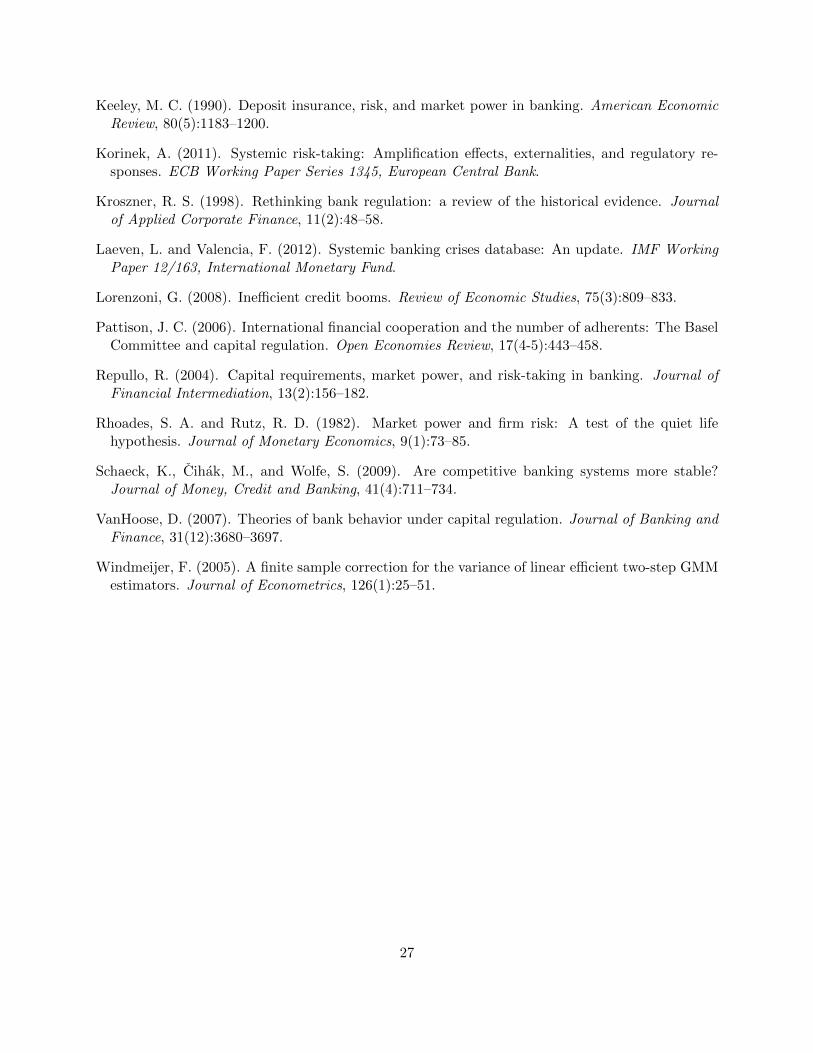
Keeley, M. C. (1990). Deposit insurance, risk, and market power in banking. American EconomicReview, 80(5):1183–1200.

Korinek, A. (2011). Systemic risk-taking: Amplification effects, externalities, and regulatory re-sponses. ECB Working Paper Series 1345, European Central Bank.

Kroszner, R. S. (1998). Rethinking bank regulation: a review of the historical evidence. Journalof Applied Corporate Finance, 11(2):48–58.

Laeven, L. and Valencia, F. (2012). Systemic banking crises database: An update. IMF WorkingPaper 12/163, International Monetary Fund.

Lorenzoni, G. (2008). Inefficient credit booms. Review of Economic Studies, 75(3):809–833.

Pattison, J. C. (2006). International financial cooperation and the number of adherents: The BaselCommittee and capital regulation. Open Economies Review, 17(4-5):443–458.

Repullo, R. (2004). Capital requirements, market power, and risk-taking in banking. Journal ofFinancial Intermediation, 13(2):156–182.

Rhoades, S. A. and Rutz, R. D. (1982). Market power and firm risk: A test of the quiet lifehypothesis. Journal of Monetary Economics, 9(1):73–85.

Schaeck, K., Cihak, M., and Wolfe, S. (2009). Are competitive banking systems more stable?Journal of Money, Credit and Banking, 41(4):711–734.

VanHoose, D. (2007). Theories of bank behavior under capital regulation. Journal of Banking andFinance, 31(12):3680–3697.

Windmeijer, F. (2005). A finite sample correction for the variance of linear efficient two-step GMMestimators. Journal of Econometrics, 126(1):25–51.

27

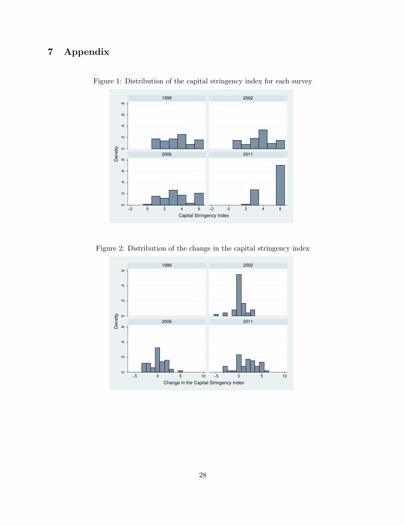
7 Appendix

Figure 1: Distribution of the capital stringency index for each survey

0.2

.4.6

.80

.2.4

.6.8

−2 0 2 4 6 −2 0 2 4 6

1999 2002

2006 2011

Density

Capital Stringency Index

Figure 2: Distribution of the change in the capital stringency index

0.2

.4.6

0.2

.4.6

−5 0 5 10 −5 0 5 10

1999 2002

2006 2011

Density

Change in the Capital Stringency Index

28

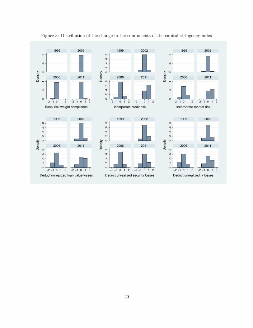
Figure 3: Distribution of the change in the components of the capital stringency index

0.5

10

.51

−2 −1 0 1 2 −2 −1 0 1 2

1999 2002

2006 2011

De

nsity

Basel risk weight compliance0

.2.4

.6.8

0.2

.4.6

.8

−2 −1 0 1 2 −2 −1 0 1 2

1999 2002

2006 2011

De

nsity

Incorporate credit risk

0.5

10

.51

−2 −1 0 1 2 −2 −1 0 1 2

1999 2002

2006 2011

De

nsity

Incorporate market risk

0.2

.4.6

.80

.2.4

.6.8

−2 −1 0 1 2 −2 −1 0 1 2

1999 2002

2006 2011

De

nsity

Deduct unrealized loan value losses

0.2

.4.6

.80

.2.4

.6.8

−2 −1 0 1 2 −2 −1 0 1 2

1999 2002

2006 2011

De

nsity

Deduct unrealized security losses

0.2

.4.6

.80

.2.4

.6.8

−2 −1 0 1 2 −2 −1 0 1 2

1999 2002

2006 2011

De

nsity

Deduct unrealized fx losses

29

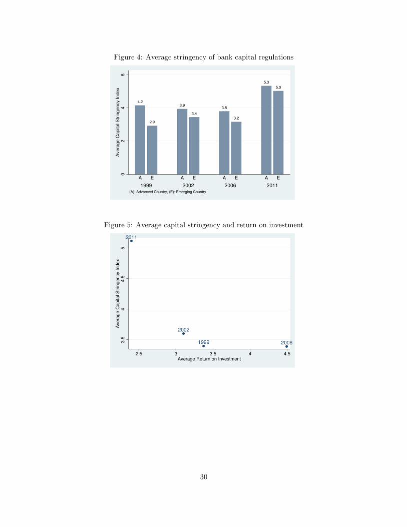
Figure 4: Average stringency of bank capital regulations

4.2

2.9

3.9

3.4

3.8

3.2

5.3

5.0

02

46

Avera

ge C

apital S

trin

gency Index

1999 2002 2006 2011

A E A E A E A E

(A): Advanced Country, (E): Emerging Country

Figure 5: Average capital stringency and return on investment

1999

2002

2006

2011

3.5

44.5

5A

vera

ge C

apital S

trin

gency Index

2.5 3 3.5 4 4.5Average Return on Investment

30

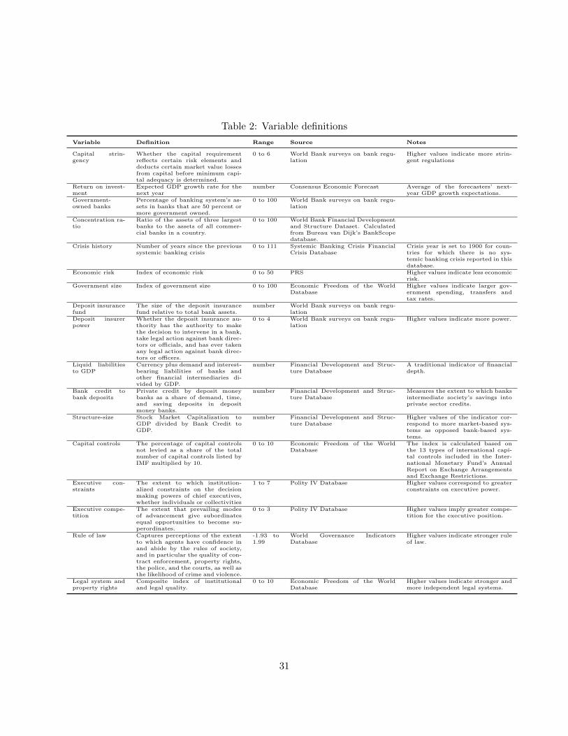
Table 2: Variable definitions

Variable Definition Range Source Notes

Capital strin-gency

Whether the capital requirementreflects certain risk elements anddeducts certain market value lossesfrom capital before minimum capi-tal adequacy is determined.

0 to 6 World Bank surveys on bank regu-lation

Higher values indicate more strin-gent regulations

Return on invest-ment

Expected GDP growth rate for thenext year

number Consensus Economic Forecast Average of the forecasters’ next-year GDP growth expectations.

Government-owned banks

Percentage of banking system’s as-sets in banks that are 50 percent ormore government owned.

0 to 100 World Bank surveys on bank regu-lation

Concentration ra-tio

Ratio of the assets of three largestbanks to the assets of all commer-cial banks in a country.

0 to 100 World Bank Financial Developmentand Structure Dataset. Calculatedfrom Bureau van Dijk’s BankScopedatabase.

Crisis history Number of years since the previoussystemic banking crisis

0 to 111 Systemic Banking Crisis FinancialCrisis Database

Crisis year is set to 1900 for coun-tries for which there is no sys-temic banking crisis reported in thisdatabase.

Economic risk Index of economic risk 0 to 50 PRS Higher values indicate less economicrisk.

Government size Index of government size 0 to 100 Economic Freedom of the WorldDatabase

Higher values indicate larger gov-ernment spending, transfers andtax rates.

Deposit insurancefund

The size of the deposit insurancefund relative to total bank assets.

number World Bank surveys on bank regu-lation

Deposit insurerpower

Whether the deposit insurance au-thority has the authority to makethe decision to intervene in a bank,take legal action against bank direc-tors or officials, and has ever takenany legal action against bank direc-tors or officers.

0 to 4 World Bank surveys on bank regu-lation

Higher values indicate more power.

Liquid liabilitiesto GDP

Currency plus demand and interest-bearing liabilities of banks andother financial intermediaries di-vided by GDP.

number Financial Development and Struc-ture Database

A traditional indicator of financialdepth.

Bank credit tobank deposits

Private credit by deposit moneybanks as a share of demand, time,and saving deposits in depositmoney banks.

number Financial Development and Struc-ture Database

Measures the extent to which banksintermediate society’s savings intoprivate sector credits.

Structure-size Stock Market Capitalization toGDP divided by Bank Credit toGDP.

number Financial Development and Struc-ture Database

Higher values of the indicator cor-respond to more market-based sys-tems as opposed bank-based sys-tems.

Capital controls The percentage of capital controlsnot levied as a share of the totalnumber of capital controls listed byIMF multiplied by 10.

0 to 10 Economic Freedom of the WorldDatabase

The index is calculated based onthe 13 types of international capi-tal controls included in the Inter-national Monetary Fund’s AnnualReport on Exchange Arrangementsand Exchange Restrictions.

Executive con-straints

The extent to which institution-alized constraints on the decisionmaking powers of chief executives,whether individuals or collectivities

1 to 7 Polity IV Database Higher values correspond to greaterconstraints on executive power.

Executive compe-tition

The extent that prevailing modesof advancement give subordinatesequal opportunities to become su-perordinates.

0 to 3 Polity IV Database Higher values imply greater compe-tition for the executive position.

Rule of law Captures perceptions of the extentto which agents have confidence inand abide by the rules of society,and in particular the quality of con-tract enforcement, property rights,the police, and the courts, as well asthe likelihood of crime and violence.

-1.93 to1.99

World Governance IndicatorsDatabase

Higher values indicate stronger ruleof law.

Legal system andproperty rights

Composite index of institutionaland legal quality.

0 to 10 Economic Freedom of the WorldDatabase

Higher values indicate stronger andmore independent legal systems.

31

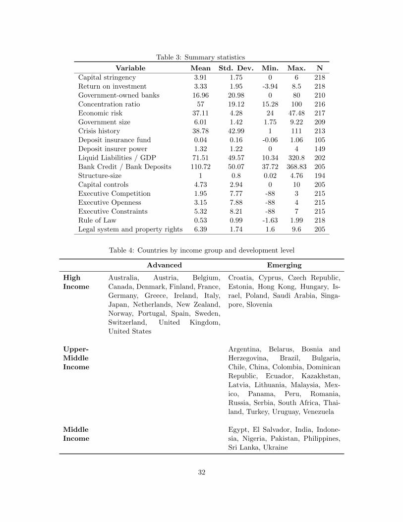
Table 3: Summary statistics

Variable Mean Std. Dev. Min. Max. N

Capital stringency 3.91 1.75 0 6 218Return on investment 3.33 1.95 -3.94 8.5 218Government-owned banks 16.96 20.98 0 80 210Concentration ratio 57 19.12 15.28 100 216Economic risk 37.11 4.28 24 47.48 217Government size 6.01 1.42 1.75 9.22 209Crisis history 38.78 42.99 1 111 213Deposit insurance fund 0.04 0.16 -0.06 1.06 105Deposit insurer power 1.32 1.22 0 4 149Liquid Liabilities / GDP 71.51 49.57 10.34 320.8 202Bank Credit / Bank Deposits 110.72 50.07 37.72 368.83 205Structure-size 1 0.8 0.02 4.76 194Capital controls 4.73 2.94 0 10 205Executive Competition 1.95 7.77 -88 3 215Executive Openness 3.15 7.88 -88 4 215Executive Constraints 5.32 8.21 -88 7 215Rule of Law 0.53 0.99 -1.63 1.99 218Legal system and property rights 6.39 1.74 1.6 9.6 205

Table 4: Countries by income group and development level

Advanced Emerging

HighIncome

Australia, Austria, Belgium,Canada, Denmark, Finland, France,Germany, Greece, Ireland, Italy,Japan, Netherlands, New Zealand,Norway, Portugal, Spain, Sweden,Switzerland, United Kingdom,United States

Croatia, Cyprus, Czech Republic,Estonia, Hong Kong, Hungary, Is-rael, Poland, Saudi Arabia, Singa-pore, Slovenia

Upper-MiddleIncome

Argentina, Belarus, Bosnia andHerzegovina, Brazil, Bulgaria,Chile, China, Colombia, DominicanRepublic, Ecuador, Kazakhstan,Latvia, Lithuania, Malaysia, Mex-ico, Panama, Peru, Romania,Russia, Serbia, South Africa, Thai-land, Turkey, Uruguay, Venezuela

MiddleIncome

Egypt, El Salvador, India, Indone-sia, Nigeria, Pakistan, Philippines,Sri Lanka, Ukraine

32

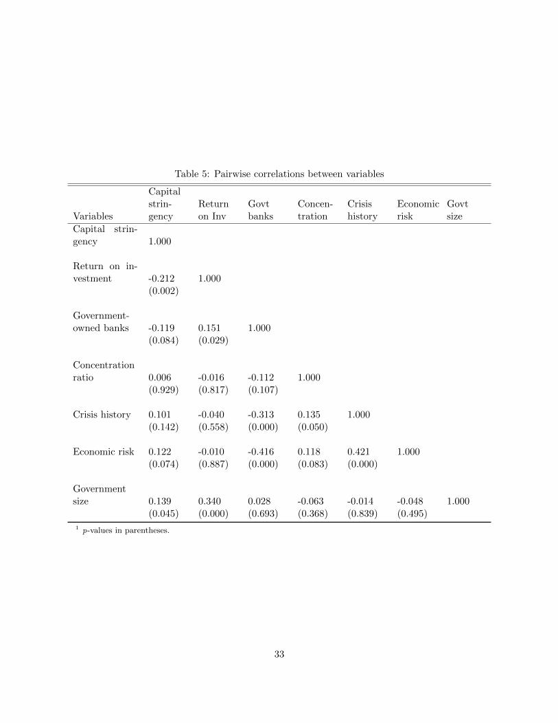
Table 5: Pairwise correlations between variables

Variables

Capitalstrin-gency

Returnon Inv

Govtbanks

Concen-tration

Crisishistory

Economicrisk

Govtsize

Capital strin-gency 1.000

Return on in-vestment -0.212 1.000

(0.002)

Government-owned banks -0.119 0.151 1.000

(0.084) (0.029)

Concentrationratio 0.006 -0.016 -0.112 1.000

(0.929) (0.817) (0.107)

Crisis history 0.101 -0.040 -0.313 0.135 1.000(0.142) (0.558) (0.000) (0.050)

Economic risk 0.122 -0.010 -0.416 0.118 0.421 1.000(0.074) (0.887) (0.000) (0.083) (0.000)

Governmentsize 0.139 0.340 0.028 -0.063 -0.014 -0.048 1.000

(0.045) (0.000) (0.693) (0.368) (0.839) (0.495)

1 p-values in parentheses.

33

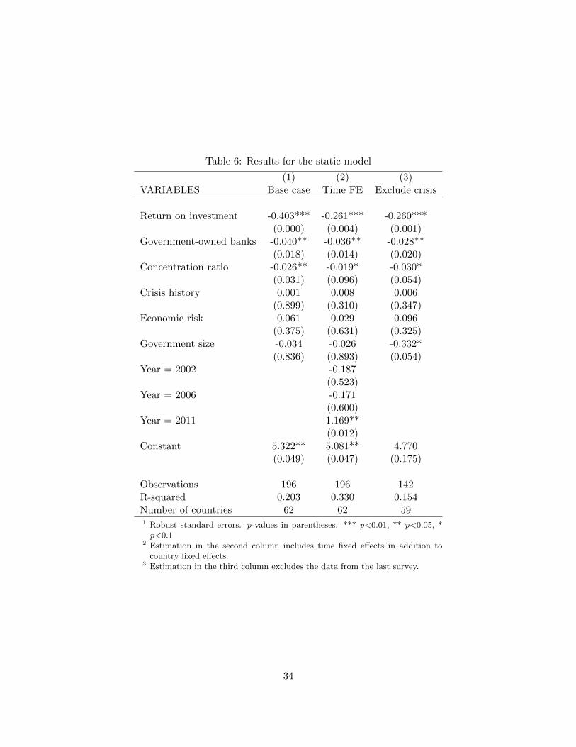
Table 6: Results for the static model

(1) (2) (3)VARIABLES Base case Time FE Exclude crisis

Return on investment -0.403*** -0.261*** -0.260***(0.000) (0.004) (0.001)

Government-owned banks -0.040** -0.036** -0.028**(0.018) (0.014) (0.020)

Concentration ratio -0.026** -0.019* -0.030*(0.031) (0.096) (0.054)

Crisis history 0.001 0.008 0.006(0.899) (0.310) (0.347)

Economic risk 0.061 0.029 0.096(0.375) (0.631) (0.325)

Government size -0.034 -0.026 -0.332*(0.836) (0.893) (0.054)

Year = 2002 -0.187(0.523)

Year = 2006 -0.171(0.600)

Year = 2011 1.169**(0.012)

Constant 5.322** 5.081** 4.770(0.049) (0.047) (0.175)

Observations 196 196 142R-squared 0.203 0.330 0.154Number of countries 62 62 591 Robust standard errors. p-values in parentheses. *** p<0.01, ** p<0.05, *p<0.1

2 Estimation in the second column includes time fixed effects in addition tocountry fixed effects.

3 Estimation in the third column excludes the data from the last survey.

34

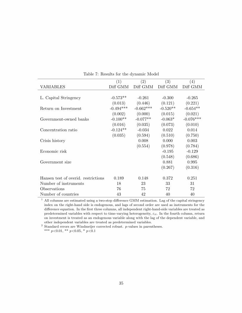
Table 7: Results for the dynamic Model

(1) (2) (3) (4)VARIABLES Diff GMM Diff GMM Diff GMM Diff GMM

L. Capital Stringency -0.573** -0.261 -0.300 -0.265(0.013) (0.446) (0.121) (0.221)

Return on Investment -0.494*** -0.662*** -0.520** -0.654**(0.002) (0.000) (0.015) (0.021)

Government-owned banks -0.100** -0.077** -0.063* -0.076***(0.016) (0.035) (0.073) (0.010)

Concentration ratio -0.124** -0.034 0.022 0.014(0.035) (0.594) (0.510) (0.750)

Crisis history 0.008 0.000 0.003(0.554) (0.978) (0.784)

Economic risk -0.195 -0.129(0.548) (0.686)

Government size 0.881 0.995(0.267) (0.316)

Hansen test of overid. restrictions 0.189 0.148 0.372 0.251Number of instruments 18 23 33 31Observations 76 75 72 72Number of countries 43 42 40 401 All columns are estimated using a two-step difference GMM estimation. Lag of the capital stringency

index on the right-hand side is endogenous, and lags of second order are used as instruments for thedifference equation. In the first three columns, all independent right-hand-side variables are treated aspredetermined variables with respect to time-varying heterogeneity, εit. In the fourth column, returnon investment is treated as an endogenous variable along with the lag of the dependent variable, andother independent variables are treated as predetermined variables.

2 Standard errors are Windmeijer corrected robust. p-values in parentheses.*** p<0.01, ** p<0.05, * p<0.1

35

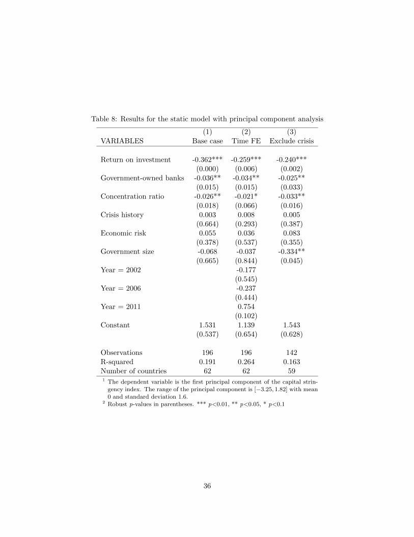
Table 8: Results for the static model with principal component analysis

(1) (2) (3)VARIABLES Base case Time FE Exclude crisis

Return on investment -0.362*** -0.259*** -0.240***(0.000) (0.006) (0.002)

Government-owned banks -0.036** -0.034** -0.025**(0.015) (0.015) (0.033)

Concentration ratio -0.026** -0.021* -0.033**(0.018) (0.066) (0.016)

Crisis history 0.003 0.008 0.005(0.664) (0.293) (0.387)

Economic risk 0.055 0.036 0.083(0.378) (0.537) (0.355)

Government size -0.068 -0.037 -0.334**(0.665) (0.844) (0.045)

Year = 2002 -0.177(0.545)

Year = 2006 -0.237(0.444)

Year = 2011 0.754(0.102)

Constant 1.531 1.139 1.543(0.537) (0.654) (0.628)

Observations 196 196 142R-squared 0.191 0.264 0.163Number of countries 62 62 591 The dependent variable is the first principal component of the capital strin-

gency index. The range of the principal component is [−3.25, 1.82] with mean0 and standard deviation 1.6.

2 Robust p-values in parentheses. *** p<0.01, ** p<0.05, * p<0.1

36

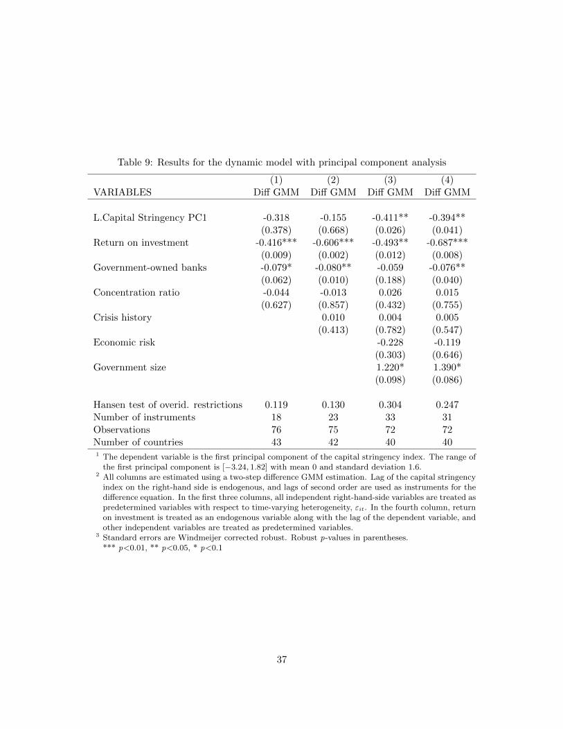
Table 9: Results for the dynamic model with principal component analysis

(1) (2) (3) (4)VARIABLES Diff GMM Diff GMM Diff GMM Diff GMM

L.Capital Stringency PC1 -0.318 -0.155 -0.411** -0.394**(0.378) (0.668) (0.026) (0.041)

Return on investment -0.416*** -0.606*** -0.493** -0.687***(0.009) (0.002) (0.012) (0.008)

Government-owned banks -0.079* -0.080** -0.059 -0.076**(0.062) (0.010) (0.188) (0.040)

Concentration ratio -0.044 -0.013 0.026 0.015(0.627) (0.857) (0.432) (0.755)

Crisis history 0.010 0.004 0.005(0.413) (0.782) (0.547)

Economic risk -0.228 -0.119(0.303) (0.646)

Government size 1.220* 1.390*(0.098) (0.086)

Hansen test of overid. restrictions 0.119 0.130 0.304 0.247Number of instruments 18 23 33 31Observations 76 75 72 72Number of countries 43 42 40 401 The dependent variable is the first principal component of the capital stringency index. The range of

the first principal component is [−3.24, 1.82] with mean 0 and standard deviation 1.6.2 All columns are estimated using a two-step difference GMM estimation. Lag of the capital stringency

index on the right-hand side is endogenous, and lags of second order are used as instruments for thedifference equation. In the first three columns, all independent right-hand-side variables are treated aspredetermined variables with respect to time-varying heterogeneity, εit. In the fourth column, returnon investment is treated as an endogenous variable along with the lag of the dependent variable, andother independent variables are treated as predetermined variables.

3 Standard errors are Windmeijer corrected robust. Robust p-values in parentheses.*** p<0.01, ** p<0.05, * p<0.1

37

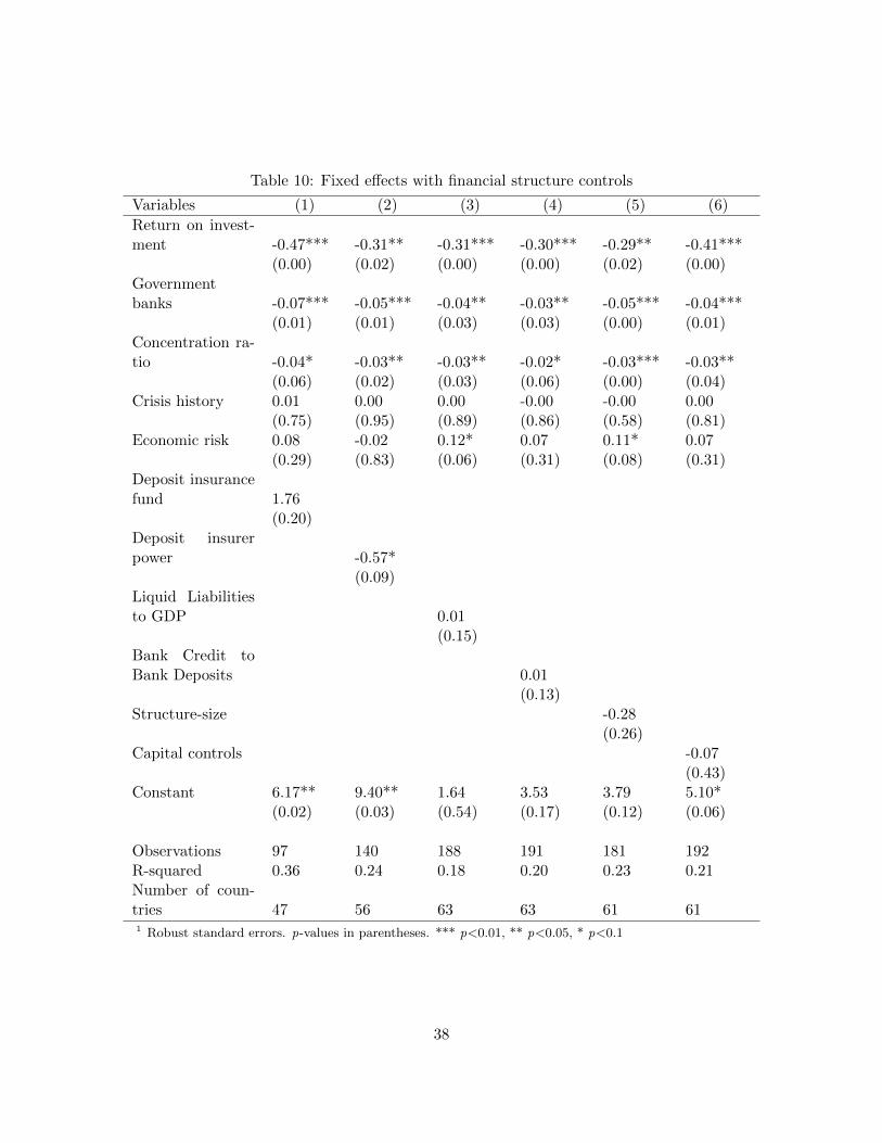
Table 10: Fixed effects with financial structure controls

Variables (1) (2) (3) (4) (5) (6)

Return on invest-ment -0.47*** -0.31** -0.31*** -0.30*** -0.29** -0.41***

(0.00) (0.02) (0.00) (0.00) (0.02) (0.00)Governmentbanks -0.07*** -0.05*** -0.04** -0.03** -0.05*** -0.04***

(0.01) (0.01) (0.03) (0.03) (0.00) (0.01)Concentration ra-tio -0.04* -0.03** -0.03** -0.02* -0.03*** -0.03**

(0.06) (0.02) (0.03) (0.06) (0.00) (0.04)Crisis history 0.01 0.00 0.00 -0.00 -0.00 0.00

(0.75) (0.95) (0.89) (0.86) (0.58) (0.81)Economic risk 0.08 -0.02 0.12* 0.07 0.11* 0.07

(0.29) (0.83) (0.06) (0.31) (0.08) (0.31)Deposit insurancefund 1.76

(0.20)Deposit insurerpower -0.57*

(0.09)Liquid Liabilitiesto GDP 0.01

(0.15)Bank Credit toBank Deposits 0.01

(0.13)Structure-size -0.28

(0.26)Capital controls -0.07

(0.43)Constant 6.17** 9.40** 1.64 3.53 3.79 5.10*

(0.02) (0.03) (0.54) (0.17) (0.12) (0.06)

Observations 97 140 188 191 181 192R-squared 0.36 0.24 0.18 0.20 0.23 0.21Number of coun-tries 47 56 63 63 61 611 Robust standard errors. p-values in parentheses. *** p<0.01, ** p<0.05, * p<0.1

38

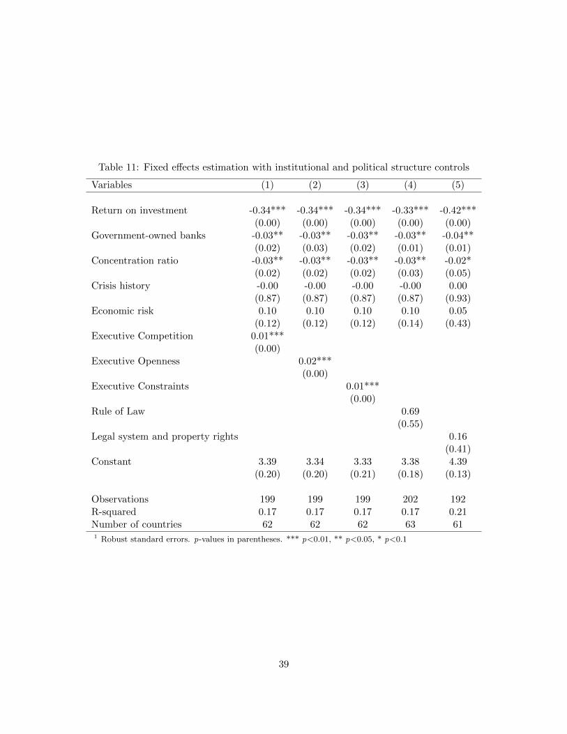
Table 11: Fixed effects estimation with institutional and political structure controls

Variables (1) (2) (3) (4) (5)

Return on investment -0.34*** -0.34*** -0.34*** -0.33*** -0.42***(0.00) (0.00) (0.00) (0.00) (0.00)

Government-owned banks -0.03** -0.03** -0.03** -0.03** -0.04**(0.02) (0.03) (0.02) (0.01) (0.01)

Concentration ratio -0.03** -0.03** -0.03** -0.03** -0.02*(0.02) (0.02) (0.02) (0.03) (0.05)

Crisis history -0.00 -0.00 -0.00 -0.00 0.00(0.87) (0.87) (0.87) (0.87) (0.93)

Economic risk 0.10 0.10 0.10 0.10 0.05(0.12) (0.12) (0.12) (0.14) (0.43)

Executive Competition 0.01***(0.00)

Executive Openness 0.02***(0.00)

Executive Constraints 0.01***(0.00)

Rule of Law 0.69(0.55)

Legal system and property rights 0.16(0.41)

Constant 3.39 3.34 3.33 3.38 4.39(0.20) (0.20) (0.21) (0.18) (0.13)

Observations 199 199 199 202 192R-squared 0.17 0.17 0.17 0.17 0.21Number of countries 62 62 62 63 611 Robust standard errors. p-values in parentheses. *** p<0.01, ** p<0.05, * p<0.1

39

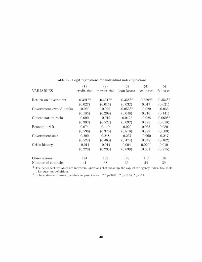
Table 12: Logit regressions for individual index questions

(1) (2) (3) (4) (5)VARIABLES credit risk market risk loan losses sec losses fx losses

Return on Investment -0.391** -0.451** -0.358** -0.389** -0.354**(0.027) (0.015) (0.032) (0.017) (0.021)

Government-owned banks -0.030 -0.029 -0.053** -0.029 -0.033(0.185) (0.209) (0.046) (0.210) (0.141)

Concentration ratio 0.000 -0.019 -0.042* -0.028 -0.060**(0.992) (0.522) (0.092) (0.325) (0.018)

Economic risk 0.074 0.110 -0.029 0.033 0.080(0.536) (0.376) (0.816) (0.799) (0.509)

Government size 0.200 0.248 -0.237 -0.060 -0.247(0.527) (0.460) (0.474) (0.848) (0.402)

Crisis history -0.011 -0.014 0.004 0.020* 0.010(0.228) (0.233) (0.639) (0.061) (0.275)

Observations 144 132 128 117 134Number of countries 41 38 36 34 391 The dependent variables are individual questions that make up the capital stringency index. See table

1 for question definitions.2 Robust standard errors. p-values in parentheses. *** p<0.01, ** p<0.05, * p<0.1

40