Bank Bailouts and Moral Hazard?

Evidence from Banks’ Investment and Financing Decisions

Yunjeen Kim ∗

November, 2013

ABSTRACT

The goal of this paper is to estimate a dynamic model of a bank to explain how bank

bailouts exacerbate moral hazard. In the model, a bank makes an endogenous choice of

the risks of its investments and can finance these investments by deposits and risky debt.

I estimate nine model parameters that characterize a bank’s behavior. For the full sample

of U.S. banks, I estimate the expected bailout probability, conditional on bankruptcy, to be

52%. The estimated conditional bailout probabilities for small and large banks are 36% and

76%, respectively. The model predicts that rescue funding constitutes 4.2% of total assets,

which is very close to the actual capital injection, 4.4% of total assets, made by the U.S.

government under the 2008 Troubled Asset Relief Program (TARP). The simulation results

show that a bank with a higher bailout belief takes more risks, especially when it is very

close to bankruptcy.

∗William E. Simon Graduate School of Business, University of Rochester, 224 Hutchison Rd., Rochester,New York, 14627. Email: yunjeen.kim@simon.rochester.edu. I would like to thank Toni M. Whited, RonKaniel, Robert Ready, Yongsung Chang, G. William Schwert, Jerold B. Warner, Lenny Kostovetsky, andRon L. Goettler for their great comments and encouragement. Additional thanks to Candace Jens, MatthewGustafson, Ruoyan Huang, and Jordan Moore for their helpful feedback.

1 Introduction

This paper examines the effects of U.S. government bailout policies on bank moral haz-

ard. Because widespread financial institution failure is generally considered to have serious

negative real effects, the U.S. government has repeatedly intervened in financial markets.

However, bank rescues in the recent financial crisis have been blamed for inadvertently in-

creasing direct costs to taxpayers, as well as increasing incentives for banks to behave in a

more risky manner. Intuitively, a bank that expects government protection takes on exces-

sively risky projects and generally acts less responsibly than it would if it had to bear the

full burden of its behavior.

The incentive effects of banks’ perceptions of bailout probabilities are thus an interesting

question, yet measuring and identifying these effects is challenging, largely because of data

limitations. First, excessive risk-taking behavior is inherently unobservable because one can-

not observe the optimal amount of risk-taking. Existing proxies, such as profit volatility,

debt-to-asset ratios, nonperforming loan ratios, and market capital-to-asset ratios, are rid-

den with measurement error, and there are no good instruments for this errors-in-variables

problem. Second, banks’ ex ante beliefs about bailout probabilities are therefore first unob-

servable, but this second problem is worse, because a bailout probability is a latent variable

with no obvious proxies.

To confront these issues, I use simulated method of moments (SMM) to estimate the

parameters of a dynamic model of a bank in order to infer bailout probabilities and the

ensuing effects on bank incentives. Structural estimation is particularly useful for addressing

the data limitation problems that accompany this inquiry. An additional advantage of this

approach is that I am able to quantify ex ante beliefs about bailouts, as well as the causal

effects of these beliefs on banks’ risk-taking.

The estimation results for the sample period 1994–2007 show that on average banks

believe that the probability of a government bailout is 52.44%. To understand whether

banks of different sizes have different ex ante bailout beliefs, I split my sample of banks by

1

size, finding that expected bailout probabilities perceived by small banks and large banks

are 35.69% and 76.20%, respectively, for the same sample period. These findings confirm

that the widespread notion that large banks perceive themselves as “too-big-to-fail.”

It is well-known that financial institutions are different from other non-financial firms

in that their capital structure and profit-making mechanisms are unique. Bank leverage

is on average much higher than that of non-financial firms. Also, most banks’ creditors

are depositors, which implies that banks have little control over this source of financing.

Moreover, a bank makes profits not by producing goods but by borrowing money at a

low interest rate and lending money at a high interest rate. Accordingly, I construct a

model that captures these distinctive properties of banks. The model features a bank that

maximizes shareholder value by determining the optimal allocation of investments and by

adjusting financing decisions. On the asset side, the bank holds cash reserves and two types of

investments: one-period risk-free bonds and risky loans. The bank’s liabilities consist of fully

insured deposits and risky debt. Debt is risky because banks have the option to default on

this debt. However, there is a possibility that in the event of default, the bank’s shareholders

will be bailed out, where the bailout consists of a cash transfer from the government sufficient

to preserve the bank’s solvency.

By estimating the parameters of this model, not only am I able to infer bailout prob-

abilities, but I am also able to characterize the differences between large and small banks.

Large banks have riskier loan investments, shorter loan maturities, lower fire-sale prices for

their assets, lower rates of return on loans, and smaller costs of adjusting their loan portfolio

than small banks. These findings are consistent with the fact that large banks have more

commercial and industrial loans and fewer personal loans.

Interestingly, the parameter that quantifies the probability of a government bailout ap-

pears crucial in allowing the model to fit the data well. I find that the moments used in my

model estimation are not well matched if the bailout belief parameter is set equal to zero but

that they are well matched if I allow this parameter to be positive. When I constrain the

2

bailout probability to be equal to zero and re-estimate the model, the parameter estimates

suggest that distressed banks be able to sell their loans at minimal discount. This result is

inconsistent with the evidence from Shleifer and Vishny (1992) and Allen and Gale (1994)

that fire-sale prices of troubled banks’ assets are well below one.

With the estimates, I also conduct counterfactual exercises. As banks move closer to

bankruptcy, they decrease their risky investments and holdings of risky debt. Banks with

beliefs of a higher bailout probability take relatively more risks on both sides of the balance

sheet, especially when they are very close to bankruptcy. That is, banks with a strong belief

decrease their risks as they approach bankruptcy but not as much as their counterparts. The

model can also assess the counterfactual effects of reserve requirements. I find that banks

invest less in loans if the reserve requirement ratio increases. Intuitively, the banks have less

money available to lend due to the larger amount of reserve requirements.

Finally, I show that the model delivers realistic out-of-sample predictions. I estimate

the model using a sample of pre-crisis data, but my simulation results show that the model

predicts surprisingly well the actual amount of rescue funds allocated by the Troubled As-

set Relief Program (TARP) of 2008. Under TARP, the Treasury injected capital into 736

financial institutions. These rescue funds amounted on average to 4.39% of total bank as-

sets. I compare this figure with the prediction from the model. In the simulated data, the

expected amount of the government’s rescue funds is about 4.21% of total assets. This pre-

diction is surprisingly close to what actually happened, given that I do not use the amount

of bailout funds to estimate the model. Thus, this out-of-sample test lets the model have

more credibility.

Three separate literatures are relevant to this paper: bank failure, government interven-

tion, and risk-taking. Whereas most papers look at each issue individually, this paper focuses

on all three simultaneously. The literature on bank failure, such as Diamond and Dybvig

(1983), Chan-Lau and Chen (2002), Caballero and Simsek (2009), He and Xiong (2009), and

Calvo (2012), identifies factors that trigger a bank-run or a financial crisis, but ignores the

3

government intervention or bank risk-taking.

There is a rich body of literature on government intervention. Schneider and Tornell

(2004), Stern and Feldman (2004), Congleton (2009), and Basu (2011) examine how govern-

ment policies affect economic conditions, yet do not consider risk-taking behavior. Wilson

and Wu (2010) and Bernardo et al. (2011) attempt to find an optimal government bailout

policy. In contrast, the the main goal of this paper is to quantify the consequences of the

government’s existing bailout policy.

This paper also falls into the literature on bank risk-taking. For example, Saunders et al.

(1990), Mailath and Mester (1994), Boyd and De Nicolo (2005), and Laeven and Levine

(2009) investigate circumstances in which a bank’s risk-taking behavior occurs. Saunders

et al. (1990) and Laeven and Levine (2009) study the relationship between risk-taking behav-

ior and ownership structure. Boyd and De Nicolo (2005) investigate a relationship between

risk-taking behavior and competition in the banking industry. Mailath and Mester (1994)

relate regulators’ policy on bank closure and the banks’ level of risks. There exists an em-

pirical literature on measuring risks of banks, such as Shrieves and Dahl (1992) and Lepetit

et al. (2008). A drawback of these studies, however, is that they employ risk proxy measures

that are only indirectly related to the risk-taking of a bank.

Only a few papers try to integrate these areas. The most closely related papers are

Cordella and Yeyati (2003), Cheng and Milbradt (2012), and Dam and Koetter (2012).

They all attempt to examine the relationship between government bailouts and moral hazard.

Cordella and Yeyati (2003) construct a model to explain the effects of a bailout policy on risk-

taking, but their analysis does not involve real data or a dynamic model. Cheng and Milbradt

(2012) mainly focus on the maturity mismatch between long-term investment and short-term

debt (as in He and Xiong (2009)). However, my focus is to explain how government bailouts

exacerbate moral hazard. In contrast to my approach of structural estimation, Dam and

Koetter (2012) adopt a reduced-form approach. Their approach requires data on risk-taking

and expected probability of bailouts, both of which are not directly observable. As an

4

alternative, they run a two-stage regression model with proxy measure of risk-taking and

political factors as instrumental variables; my approach requires neither any proxy measure

of risk-taking nor expected probability of bailouts. The structural estimation adopted in

this paper also allows me to estimate the expected probability of bailouts and to explore

counterfactuals.

The paper is organized as follows. Section 2 describes the model. Section 3 describes

the data and the estimation procedure. Section 4 presents the estimation results. In Section

5, I present the counterfactuals. Section 6 contains the out-of-sample test. In Section 7, I

investigate the ex ante belief about bailout probabilities. Section 8 concludes. The Appendix

contains details concerning the model solution.

2 Model

Banks differ from non-financial firms in their capital structures and profit-making mecha-

nisms. Commercial banks borrow money on a short-term basis in the form of consumer

deposits, which can be withdrawn at any time. The major assets for most banks are mort-

gages (real estate loans), credit card loans, auto loan receivables, and business loans, all of

which are illiquid and have long maturities. Banks make profits by borrowing money at a

low interest rate and lending money at a high interest rate. Banks adjust their assets and

liabilities to generate profits. Figure 1 shows a typical U.S. commercial bank’s balance sheet

with assets on the left side, and liabilities and net worth on the right side. The percentages

in parentheses are the actual averages of each category for commercial banks in the U.S. from

1987 to 2008. The sample is from the Reports of Condition and Income, Bank Regulatory

Database.

[Insert Figure 1]

A bank has four main categories of assets: loans, securities, cash reserves, and physical

assets. More than half of a bank’s assets are loans, which are the primary source of interest

5

revenue. Types of loans include loans to consumers (home loans, personal loans, auto loans,

credit card loans) and businesses (real estate development loans, capital investment loans).

About 30% of a bank’s assets are investment securities. Investment securities include U.S.

Treasury securities and federal funds. Securities are safer than loans, but they do not pay

as much interest as loans do. Securities are not as safe as cash reserves, but they pay

more interest than cash reserves. Cash reserves represent about 10% of a bank’s assets,

and they include vault cash and Federal Reserve deposits, which typically constitute reserve

requirements. In the U.S., the Board of Governors of the Federal Reserve System sets

reserve requirements, which apply to some deposits held at depository institutions, such as

commercial banks, savings and loan associations, savings banks, and credit unions. Last,

physical assets include buildings, land, and equipment owned by the bank. This category is

relatively small for most banks.

On the other side of the balance sheet are net worth and liabilities. The average leverage

of commercial banks is 90%, which is extremely high compared to non-financial firms. The

liabilities mostly consist of deposits, suggesting that banks have little control over the liabil-

ity side. There are two ways to consider the types of deposits. The first way is by the length

or accessibility of deposits: demand deposits (or transaction deposits) and time and savings

deposits. Demand deposits include all deposits in depository institutions that can be with-

drawn without prior notice, and savings deposits are locked up for a certain length of time.

The second classification divides deposits into insured and uninsured deposits. Between 1980

and 2008, the Federal Deposit Insurance Corporation (FDIC) insured a depositor’s accounts

up to $100,000 for each deposit ownership category in each insured bank; the deposit insur-

ance limit was increased to $250,000 on October 3, 2008. The remaining 10% on the balance

sheet is net worth, or what the bank owes the equity holders. A negative net worth would

put the bank in default.

A bank can therefore be characterized by its balance sheet. The key features of the

model proposed in this paper are summarized as follows: (i) on the asset side, there are cash

6

reserves and two types of investments: a one-period risk-free bond, bt, and a portfolio of

risky loans, lt; (ii) on the liability side, there are fully-insured, exogenously-given deposits,

dt, and fairly-priced risky debt, qt; (iii) a bank goes bankrupt if its net worth wt is less

than 0, but it believes the government would bail it out with probability η; (iv) a bank

maximizes shareholder value by choosing the investment (bt and lt) and financing decisions

(qt); (v) shareholders are risk-neutral; and (vi) time is discrete and the horizon is infinite.

In addition, the bank’s balance sheet should be balanced:

lt + bt = wt + dt + ptqt, (1)

where pt is the price of the risky debt qt. In each period of time, a bank with an infinite hori-

zon optimizes over three decision variables q′, l′, b′ given six state variables q, l, b, d, d′, z,

where variables with primes denote the next period’s values. The following subsections de-

scribe how the model is constructed to resemble the properties of a generic balance sheet of

a bank.

2.1 Asset Side

On the asset side, a bank invests in a risk-free bond, b, which yields a risk-free rate of return,

rf . The bank also invests in a portfolio of risky loans, l, which yields a rate of return, rl. A

fraction of the loans, δ, is due in each period; δ < 1 indicates that the average loan maturity

is longer than one year. There is a risk that the loans can default; z denotes the survival rate

of loans, implying that 1− z of loans default in each period. Defaulting is independent from

maturing. Thus, the income from loans consists of two components: a stochastic survival

rate, z, and a deterministic profitability rate, rl. Investing an amount of l in a portfolio of

loans yields (rl + δ)zl in the following period. The remainder, (1− δ)zl, is rolled over to the

7

next period. The law of motion of l is therefore given by:

l′ = (1− δ)zl + i, (2)

where i is the amount of new loans that are invested at time t for the next period. The

survival rate z of loans has a truncated-normal distribution (see Appendix B for details):

ziid∼ N(µz, σ

2z), z ∈ [0, 1]. (3)

The bank also holds cash reserves as required by the Board of Governors of the Federal Re-

serve System. The reserve requirement is denoted by α. The cash reserves are automatically

determined by the deposits. The available capital for investments at time t is At−αdt, where

At is total assets and dt is deposits held by the bank.

2.2 Liability Side

On the liability side, a bank borrows money from depositors, called “deposits,” d. The

deposits are random in each period; the bank cannot choose how much it wants to borrow

from depositors. The deposits, d, follow an AR(1) process:

d′ = µd + ρdd+ εd, (4)

where εd ∼ N(0, σ2d). All deposits are fully insured. d corresponds to the insured deposits in

Figure 1 and is referred to as deposits instead of insured deposits hereafter. The depositors

require a fixed per-period interest rate, rd, which is lower than the risk-free rate (i.e., rd < rf ),

as in De Nicolo, Gamba, and Lucchetta (2011). The difference between the two rates includes

costs of the intermediary’s service, as well as costs of the insurance.

The bank can also issue debt, q′, which is risky, because the bank can default on the

8

debt. The bank’s cash balance at the beginning of the next period is given by:

c′ = (rl + δ)z′l′ + (1 + rf )b′ − (1 + rd)d

′ − q′ + αd′. (5)

The first two terms in Equation (5) are the incomes from risky loans and risk-free bond

investments. The next two terms are the payments to the depositors and debt holders. The

last term is the cash reserves determined by deposits held at the bank.

The bank is financially distressed if its cash balance, c, is less than zero after the credit

shock, z, is realized but before the new deposits, d′, are given. A financially distressed bank

does not necessarily exit the market. Financial distress (cash default) occurs when a bank

does not have enough cash to pay back outstanding debt. When a bank has insufficient cash,

it sells its existing loans at a fire-sale price, ξ, to meet its debt obligations. The distressed

bank needs to sell only cξ

of its loans. After the fire-sales, the net worth becomes:

w = (1− δ)zl +c

ξ, (6)

if any. If w is negative, the bank files for bankruptcy. At this point, the bank is reorganized

through Chapter 11 bankruptcy protection, in which the reorganization process imposes

costs on shareholders.

The distress threshold can be represented by a function of the survival rate, z, as in

Gilchrist, Sim, and Zakrajsek (2010). The bank is in financial distress when z < zd, where:

zd(b′, q′, l′; d′) ≡ (1 + rd)d

′ + q′ − αd′ − (1 + rf )b′

(rl + δ)l′. (7)

In the event of financial distress, the recovery of the debt holders, R(·), is:

R(b′, q′, l′; d′, z′) = max

min

(rl+δ)z′l′+ξ(1−δ)z′l′+(1+rf )b

′−(1+rd)d′+αd′, q′

, 0, (8)

9

where ξ is a fire-sale price of outstanding loans. Since loans are illiquid, the sale price of the

loans is less than 1. Thus, the debt-pricing formula, p(·), is given by:

p(b′, q′, l′; d′) =1

1 + rd

(1 +

∫ zd

z

[R(b′, q′, l′; d′, z′)

q′− 1]dΦ(z′)

). (9)

This equation implies that debt holders’ and depositors have the same expected profits as

in Hennessy and Whited (2007) and Gilchrist, Sim, and Zakrajsek (2010).

2.3 Bankruptcy and Government Intervention

In the event of bankruptcy, the government can intervene and rescue the troubled bank. I

assume that the bailout decision is random and constant from a bank’s perspective. The

bank has ex ante belief η about the probability of government intervention conditional on

bankruptcy. If the government rescues a bank, it injects capital, τ , into the bank to prevent

the bank from having to sell its loans at fire-sale prices.

In the real world, the capital injection in a bailout can take several forms, such as loans,

stocks, bonds, or cash. During the recent financial crisis, the Treasury bought troubled

assets – especially mortgage-backed securities – of domestic financial institutions, and it also

bought equity positions in the largest banks in the U.S. using taxpayer funds. In addition to

purchasing troubled assets or stocks, another type of bailout occurs in the form of regulatory

mergers, which are very common in financial markets but often ignored.

When federal bank regulators get involved with an insolvent bank or financial institution,

they can take two types of action. First, the FDIC can become the receiver of a failed bank

and enters a liquidation process like a bankruptcy trustee. In such a case, the FDIC closes

down the bank, pays off depositors up to the insurance limit ($250,000 since 2008), and

sells off the assets. Shareholders of the failed bank can expect to suffer losses. Second, and

more commonly, the FDIC finds a healthy bank to merge with or buy the failed bank. The

regulators often entice the acquiring bank with subsidies or relaxed capital requirements.

10

Thus, a merger between two banks arranged by financial regulators can be thought of as a

bailout or government help.

Table I contains the number of FDIC-approved bank mergers every year between 2000 and

2010. There are four categories of bank mergers: regular merger, corporate reorganization

merger, interim merger, and probable failure or emergency merger. Unfortunately, the data

on the regulatory mergers are not available. The table also includes the total number of

banks as well as the number of failed banks. The total number of banks comes from the

Bank Regulatory Database. Table I shows that there have been a number of mergers over

the last decade. On average, about 4% of banks are acquired by another bank each year.

Only a few banks have actually failed.

[Insert Table I]

2.4 Bank Problems

Figure 2 summarizes a bank’s problems from time t to time t + 1. The bank has chosen

the risk-free bond b, loans l, and risky debt q during the previous period, t − 1. At the

beginning of time t, the bank observes its deposits d and the loan survival rate, z. These

shocks determine whether or not the bank becomes financially distressed. If the bank’s cash

balance is positive, the bank can continue by choosing a new financing decision, q′, and new

investment decisions, b′ and l′, given the new deposit level, d′. If the cash balance is negative

and thus the bank is in cash default, then the bank sells its loans to fulfill its debt obligations.

If it is not feasible to pay back the outstanding debt even after the bank sells all its existing

loans, the bank files for bankruptcy. Once a bank files for bankruptcy, the government

intervenes and bails it out with probability η. Otherwise, the bank is reorganized, and

associated costs are levied on shareholders.

[Insert Figure 2]

11

There are asymmetric adjustment costs for loans. Increasing the loan amount could be

costly for a bank due to monitoring. The adjustment costs, Λj, for each case j ∈ C ≡

Continuation, D ≡ Distress, B ≡ Bailout are given by:

Λj = λ(x− l′)21l′ > x, j ∈ C,D,B, (10)

where λ is a coefficient of the adjustment cost function of loans and x is the remaining loan

amount after fire-sales, if necessary. Cash flows to shareholders are reduced by the loan

adjustment costs.

Let ej be cash flows to shareholders after choosing the next-period financing and in-

vestment decisions in each case j ∈ C,D,B. When cash balance c is positive, the bank

continues by choosing the new financing and investment decisions, and cash flows to share-

holders are given by:

eC = c+ (1− δ)zl + (1− α)d′ − l′ − b′ − ΛC + p(b′, q′, l′; d′)q′. (11)

In such a case, the remaining loans, x, are (1− δ)zl, since the bank does not need to sell any

of its existing loans. The bank first realizes its cash balance plus remaining loans plus new

deposits. The bank has to maintain some of its deposits as cash reserves. The bank then

chooses new investments in risky loans and a risk-free bond, and it pays adjustment costs

if it increases its loan investments. Finally, the bank can raise money by issuing debt at a

price p(·).

When cash balance c is negative, the bank sells its outstanding loans at a fire-sale price,

ξ, until it can meet its debt obligations. If c+ ξ(1− δ)zl is positive, the bank does not need

to sell all its loans. In this case, the bank needs to sell just enough of its existing loans, | cξ|,

to meet its debt obligations. The cash flows to shareholders in this case are given by:

eD =c

ξ+ (1− δ)zl + (1− α)d′ − l′ − b′ − ΛD + p(b′, q′, l′; d′)q′. (12)

12

After the fire-sales, the bank is left with x = cξ

+ (1− δ)zl of loans.

A bank may still be unable to meet its debt obligations even after selling all of its loans. In

that case, the bank files for bankruptcy and the debtors enter a reorganization process. The

debtors have all ex post bargaining power and extract all bilateral surplus. All reorganization

costs are passed along to shareholders, therefore the cash flows to shareholders are the same

as in Equation (12). In the event of bankruptcy, however, the government may intervene

and bail out the troubled bank with probability η. Once the government decides to rescue

the troubled bank, it injects cash τ and cash flows to shareholder are:

eB =c+ τ

ξ+ (1− δ)zl + (1− α)d′ − l′ − b′ − ΛB + p(b′, q′, l′; d′)q′. (13)

The government essentially cancels out the negative cash balance c with τ .

Therefore, at each time t, a bank chooses qt+1, bt+1 and lt+1 that maximize discounted

lifetime expected equity value given the set of states, qt, bt, lt, dt, dt+1, zt. The objective

function of the bank’s shareholders is given by:

maxqh+1,bh+1,lh+1,h=t,··· ,∞

Et[ ∞∑k=t

βk−tejt

], j ∈ C,D,B, (14)

where β is a discount factor. As six state variables create computational complications,

simplifying assumptions are made in the following section.

2.5 Model Simplification

I assume that a bank chooses the investment decisions, l′ (or i) and b′, and the financing

decision, q′, after observing the income from loans (the credit shock z), but before the next-

period deposits d′ are realized. The bank thus makes financing and investment decisions

based on the expected value of next-period deposits. According to the AR(1) process of

13

deposits, the expected value of d′ conditional on d is given by:

E[d′|d] = µd + ρdd, (15)

which is a function of the current level of deposits. The debt pricing formula in Equation

(9) then becomes

p(b′, q′, l′; d) =1

1 + rd

(1 + E

[ ∫ zd

z

[R(b′, q′, l′, d′, z′)

q′− 1]dΦ(z′)

∣∣∣d]). (16)

There are two advantages of this assumption. First, the number of state variables is reduced

by 1; the state variables are now q, l, b, d, z, which simplifies the computations. Second,

the assumption introduces uncertainty about the level of deposits, which can be interpreted

as rollover risk.

I further assume that the total assets, A, are fixed at 1. The fixed total capital assumption

can be justified, because risk-taking is not determined by the total size of investment but by

the allocation between the risky loans and the risk-free bond. As discussed in Section 2.1,

the available assets for investment are A − αd per the reserve requirements. Choosing the

amount invested in loans automatically determines the amount that should be invested in

the risk-free bond, and vice versa (i.e., b = A−αd− l). This assumption eliminates one state

variable and one choice variable. Therefore, there are two decision variables q′, l′ and four

state variables q, l, d, z.

The last assumption is not related to computation but to empirical identification of the

parameters. I assume that the cash injection made by the government τ is equal to |c|, the

amount of money that the troubled bank lacks. When the net worth after the fire-sale of

loans, w = cξ

+ (1− δ)zl, is negative, the bank files for bankruptcy. With the government’s

cash injections of τ = |c|, sufficient to supplement the existing loan amount of (1 − δ)zl,

preventing the bank from entering a fire sale. These cash injections allow creditors to recoup

their money from the bank, or, more accurately, from the government. This simplifying

14

assumption is necessary, because the government bailout probability parameter η and the

cash injection parameter τ cannot be identified simultaneously. From a bank’s point of view,

the model is solved based on its expectation about a bailout, which is the product of η and

τ .

In sum, the Bellman equations in each case are given by:

V j(q, l, d, z) = maxq′,l′

ej + βE[V (q′, l′, d′, z′)|d]

, j ∈ C,D,B. (17)

In each period, a bank chooses its investment decision, l, and financing decision, q, given

deposits, d, and credit shock, z. There are four possible outcomes: the bank continues, the

bank is financially distressed, or the bank files for bankruptcy, in which case it may or may

not get bailed out. For each case, the value function is defined as follows:

V (q, l, d, z) =

V C(q, l, d, z) if c ≥ 0,

V D(q, l, d, z) if c < 0 and w ≥ 0,

ηV B(q, l, d, z) + (1− η)V D(q, l, d, z) if c < 0 and w < 0,

(18)

where c is the bank’s cash balance and w is its net worth after fire-sales if necessary. The

model solutions are described in Appendix A in detail.

3 Estimation

3.1 Estimation Outside of the Model

Table II reports all of the model parameters. Most of the parameters in the model are

estimated using simulated method of moments (SMM). However, some of the parameters

are estimated separately. The risk-free rate rf is the annualized one-month Treasury-bill

return and is set equal to 3%.1 The market discount factor β is then equal to 11+rf

. The rate

of return on deposits, rd, is set to 1%. The sources for rd are the national one-year CD rate,

1The source for Treasury-bill returns can be found at http://mba.tuck.dartmouth.edu/pages/

faculty/ken.french/Data_Library/.

15

the national money market accounts rate, and the checking account interest rate during the

sample period. The default rate of loans, 1−µz, is the average of the sum of charge-off rates

and delinquency rates on loans and leases of all commercial banks in the U.S. provided by

the Board of Governors of the Federal Reserve System, and it is 4% over the sample period.

The Federal Reserve currently sets the depository institution’s reserve requirements at

10% of net transaction accounts if the net transaction accounts exceed $79.5 million. If net

transaction accounts are between $12.4 million and $79.5 million, the reserve requirement

ratio is 3%, and if net transaction accounts are less than $12.4 million, there is no reserve

requirement. Since data on net transaction accounts are not available, I assume that cash

reserves are determined by insured deposits, d, instead of net transaction accounts in the

model. As shown in Figure 1, U.S. commercial banks hold 10% of their insured deposits as

cash reserves, and thus α is set at 10%. Panels A and B of Table II summarize the set of

parameter values estimated outside of the model.

[Insert Table II]

3.2 Estimation by SMM

There are nine model parameters: the drift and serial correlation of the deposits process,

µd and ρd; the standard deviation of the shock to deposit process, σd; the conditional belief

of the probability of government bailout, η; the standard deviation of the loan survival

rate, σz; the fire-sale price of existing loans, ξ; the percentage of loans that mature in each

period, δ; the rate of return on loans, rl; and the loan adjustment cost coefficient, λ. These

model parameters are estimated using simulated method of moments (SMM), which chooses

parameters so that the distance between the moments of the real data and the moments of

the simulated data is as small as possible. The data used for the SMM are described in the

following section.

The deposit process can be estimated separately from the model. In contrast, I follow

the two-step procedure, proposed by Cooper and Haltiwanger (2006), in which the param-

16

eters are split into two sets. The first set includes the three parameters generating the

deposit process (Θ1 ≡ µd, ρd, σd) and the second set contains the other six parameters

(Θ2 ≡ η, σz, ξ, δ, rl, λ). Given initial values for the second set of parameters, Θ02, the three

parameters related to deposits in Θ11 are estimated by matching three moments: the aver-

age, serial correlation, and standard deviation of deposits. Using the estimates of the deposit

process, the second set of six parameters is estimated and denoted by Θ12. To identify this

set of parameters, nine moments are chosen to be matched. The moments and the details

for the identification strategies are described in Section 3.4. When the nine moments are

matched, the three moments related to deposits are then re-calculated using the six param-

eters that have been found so far. If these moments are sufficiently close to the moments in

the first step, the procedure stops. If the given moments are not close enough, the first set of

parameters is re-estimated, given Θ12, and denoted by Θ2

1. The process is repeated until the

moments related to deposits are matched. Since deposits are exogenously given and they, in

turn, are independent from other parameters, one iteration is sufficient to estimate all the

parameters.

The hypothetical banks generated by the model are heterogeneous only in terms of their

shocks. The SMM’s function is to estimate the parameters of an average bank. The real

bank data, however, are heterogeneous across many dimensions. Thus, when using the

SMM, it is critical to eliminate as much heterogeneity from the data as possible. Firm fixed

effects are used in the estimates of variance. In addition, the double-differencing method of

Han and Phillips (2010) is used to determine the AR(1) coefficients. Further, the sample

is split into two subsamples – small and large banks – and the model is estimated for each

subsample. Another reason to estimate the subsamples by size is to see whether large banks

have a stronger belief than small banks that the government will bail them out, in other

words, that they are “too-big-to-fail”. This point will be examined later in this paper.

Figure 3 plots the yearly cross-sectional averages of several variables for banks in a sample

of commercial banks between 1994 and 2007. Panel A plots the total liabilities, insured

17

deposits, loans, and operating income for the full sample. Panels B and C plot the variables

for small banks and large banks, respectively. The figures show that small banks and large

banks are different.

[Insert Figure 3]

When minimizing the objective function, a weighting matrix with firm fixed effects is

used. The standard errors are calculated using a clustered weighting matrix. According to

Erickson and Whited (2000), the weighting matrix is the inverse of the sample variance-

covariance matrix of the moments, which is the inner product of stacked influence functions

of the moments. More details about how to implement SMM are described in Appendix C.

3.3 Data

The data are from the Reports of Condition and Income (Call Reports), Bank Regulatory

Database of the Federal Reserve Bank of Chicago, which provides quarterly accounting data

for commercial banks. The sample period is from 1994 to 2007. The sample ends in 2007

because the database provides the amount of deposits greater than $100,000, while the de-

posit insurance limit has been increased to $250,000 since October 3, 2008. Data variables

are defined as follows: total assets is RCFD2170 ; debt is RCFD2950 ; operating income is

RIAD4000 ; distributions to shareholders is RIAD4460 (common stock) plus RIAD4470 (pre-

ferred stock) minus negative RIAD4346 (net sale of stock); and insured deposits is RCFD2200

(total deposits) minus RCON2710 or RCONF051 (deposits greater than $100,000).

Observations in which total assets are less than $1 million or operating income or deposits

are non-positive are deleted from the sample. As some variables are only available on an

annual basis, the quarterly data are annualized. Flow variables are accumulated from the

first quarter to the fourth quarter of each fiscal year. Stock variables are the fourth quarter’s

values. If there is a missing value in any quarter, the bank-year observation is dropped. All

variables are deflated by the annual total assets. Observations are included only when at

18

least three consecutive years of data are available. Winsorizing the top and bottom 1% of

the variables produces an unbalanced panel of banks from 1994 to 2007, with between 7,597

and 10,948 observations per year, and 123,159 bank-year observations. The data reveal that

the number of banks in the market monotonically decreases over time.

The bankruptcy frequency is calculated by dividing the number of banks that are delisted

from the FDIC database for a given year by the total number of banks that are listed in the

FDIC database in the previous year:

Bankruptcy Frequency =(# of banks in t)− (# of banks in t− 1)

(# of banks in t− 1). (19)

Note that (# of banks in t) does not take into account newly entering banks in year t.

3.4 Identification

The objective of the SMM procedure is to determine the values of the model parameters

that minimize the distance between the simulated moments and the actual moments. Since

model identification is critical in this procedure, it is necessary to choose the moments

carefully; the mean, variance, and autocorrelation of all possible variables are computed and

reveal the moments that are most sensitive to variation in parameter values. The three

parameters related to the deposit process, µd, ρd, σd, are identified by the three moments

of the actual deposit process. The other six parameters, η, σz, ξ, δ, rl, λ, that characterize

a bank’s behavior are determined by matching nine moments: the first moment of leverage,

the autocorrelation of leverage, the standard deviation of the shock to leverage, the first

moment of operating income, the first moment of dividends, the first and second moments of

charge-offs, the ratio of insured deposits to total liabilities, and the frequency of bankruptcy.

Identifying the expectation about government bailout probability, η, is crucial for this

study. The most informative moments for this parameter are the ratio of insured deposits

to total liabilities and the bankruptcy frequency. In the model, the deposits are exogenously

19

given, but banks can choose additional borrowing by paying an appropriate price. In ad-

dition, as shown by Figure 3, insured deposits decrease monotonically over time, but total

liabilities are stable, forming around 90% of total assets. This trend implies that banks

are borrowing more risky debt in order to maintain the high level of leverage, which leads

a higher level of risks. The bailout belief parameter can thus be identified by the ratio

of insured deposits to total liabilities. The bankruptcy frequency is also of great use for

identifying the parameter η. Intuitively, more banks would go bankrupt if they believe that

government bailouts are more likely, since the higher belief in bailouts induces banks to take

more risks.

The other parameters are standard. The first moments of operating income and dividends

help establish the rate of return on loans, rl. As the rate of return on loans increases, banks

become more profitable. When banks profit from high rates of return of loans, they can then

pay out higher dividends. Choosing the appropriate moments of leverage helps identify the

average maturity, δ. If the maturity of loans were too short, the leverage would be unstable.

The adjustment cost coefficient affects the charge-offs as well as bank income. If banks have

difficulty adjusting their loan investments, the loan amounts will not change frequently or

promptly. The standard deviation of the charge-offs is directly affected by the standard

deviation of the survival rate of the loans, σz. The fire-sale price, ξ, affects the bankruptcy

frequency. Even if a bank cannot meet its debt obligations, and if it can sell existing loans

at a higher price, it might be able to alleviate its financial distress. Panel C of Table II

contains the parameters to be estimated using SMM with most informative moments.

4 Estimation Results

4.1 Full Sample

Table III contains estimation results for the full sample. Panel A reports both the actual

moments and the simulated moments with t-statistics that accompany the difference between

20

the actual and simulated moments. The three moments related to the deposit process are

almost perfectly matched to the data moments. Fewer than half of the simulated moments

are statistically significantly different from their real-data counterparts. The model fits the

average of leverage, the average of income, the average of charge-offs, the deposit ratio, and

the bankruptcy frequency particularly well. The model fails to match the first moment of

dividends because the model does not include taxes.

[Insert Table III]

Panel B of Table III reports the parameter estimates with clustered standard errors in

parentheses. The belief in the bailout probability conditional on bankruptcy is estimated to

be 52.44%, which is lower than Dam and Koetter’s (2012) estimate of 69%. Recall that Dam

and Koetter (2012) run a two-stage regression. In contrast to the structural estimation used

in this paper, their methodology requires a proxy for risk-taking and instrumental variables

for the latent variable, the expected bailout probability. The structural estimation adopted

in this paper also allows me to explore counterfactuals. The estimated fire-sale price is

46.42%, which is lower than that of non-financial firms (e.g. Hennessy and Whited (2005)

estimate it at 59.2%). This estimate suggests that investments in loans are generally illiquid.

On average, 69% of loans mature in each period. One period in the model is equal to one

year, and therefore the average maturity of loans is about 525 days. The estimated value of

the average maturity is close to the weighted-average maturity for commercial and industrial

(C&I) loans of all U.S. commercial banks in the same period, which is about 469 days. The

rate of return on loans is about 11%, which is consistent with the actual data. The rate rl

serves as a required rate of return on a portfolio of loans in order to account for multiple

types of loans. For instance, over the same period, the average 30-year fixed mortgage rate

is 7%; the finance rate on consumer installment loans at commercial banks is 8%; the finance

rate on personal loans at commercial banks is 13%; and the interest rate on credit card plans

of commercial banks is 14%. Thus, the rate of return on commercial bank loans should be

close to the weighted average of these rates.

21

4.2 Subsamples

In the model, a bank believes that the government will bail it out in case of failure. The

model and its parameters explain an average bank’s behavior. On the other hand, the U.S.

government’s rescue programs appear to have been applied on an ad hoc basis with varying

degrees of taxpayer support. For instance, in the recent financial crisis, the U.S. government

rescued Bear Stearns by subsidizing its merger with JPMorgan Chase & Co. The U.S.

Treasury took over Fannie Mae and Freddie Mac. The Federal Reserve injected capital

directly into American International Group, Inc. At the same time, the government declined

to help Lehman Brothers Holdings Inc., and the company eventually filed for Chapter 11

bankruptcy protection (Ayotte and Skeel Jr. (2010)).

Despite the varying degrees of assistance offered to financial institutions by the U.S.

government, the likelihood of a government bailout seems to increase in the size of a bank;

large banks are deemed too big to fail. Since a big bank is connected to many financial

and non-financial firms, the failure of the big bank may have a domino effect, potentially

affecting both the national and global economies (Aharony and Swary (1983)).

To investigate the idea that some banks are too big to fail, the sample is split by size (small

vs. large banks), and the expectation of bailout probability is estimated for each subsample.

Tables IV and V show the estimation results for small and large banks. “Bank size” is defined

as total assets: small (large) banks are in the lower (higher) third of the distribution of total

assets in each year. The estimation method is identical to that described in Section 4.1. The

moments related to the deposits are different for each subsample. As shown in Figure 3, the

mean ratio of insured deposits to total liabilities is higher for large banks (64.97%) than for

small banks (53.10%). Thus, the parameters related to the deposit process are re-estimated

for each subsample. The estimation results show that the drift and serial correlation of the

deposit process for small banks are slightly higher than those for large banks. Additionally,

the standard deviation of shocks to the deposit process is higher for large banks than for

small banks.

22

[Insert Table IV]

[Insert Table V]

Panel B in Tables IV and V refers to the parameters governing a bank’s behavior. When

comparing small and large banks, several notable differences in parameter estimates emerge.

The first is the ex ante bailout probability. This probability is estimated as 76.20% for large

banks and 35.69% for small banks. Compared to small banks, large banks believe more

strongly that the government will bail them out if they are in trouble, which implies that

large banks perceive themselves too big to fail. Second, the fire-sale prices indicate that

small banks can sell their existing loans at a higher price than large banks. At the same

time, according to the adjustment cost coefficient, large banks can increase loan holdings

more easily than small banks. Third, the average maturity of loans is slightly longer for

small banks (568 days) than for large banks (515 days). The average maturity of C&I loans

is shorter than that of personal loans, and therefore these estimates of maturity reflect the

fact that large banks hold more C&I loans and fewer personal loans than do small banks.

Finally, the rate of return on loans for large banks is lower than for small banks, but the

standard deviation of the loan survival rate is slightly higher for large banks than for small

banks. If large banks believe that they are more likely to benefit from a bailout, then they

may be more likely to invest in riskier or less profitable loans.

5 Counterfactuals

In this section, two counterfactual exercises are conducted by simulating the model, with

the parameter values estimated for the full sample by SMM. The first exercise analyzes how

the sensitivity of a bank’s behavior to the bailout belief parameter η depends on the bank’s

health. The second exercise shows how a bank reacts to changes in the reserve requirement

rate. Let η denote the estimated value of the government bailout belief parameter η from

Table III, hereafter referred to as “the original belief.”

23

5.1 Distance from Bankruptcy

A bank’s behavior depends not only on its belief about government bailouts but also on its

health. First, the expectations of future government bailouts may affect a bank’s decision

making. For example, a stronger belief about the possibility of a government bailout may

induce the bank to behave irresponsibly. Second, the bank’s behavior may also depend on

the bank’s health. Health, in this context, refers to the bank’s distance from bankruptcy. If

a bank is far from bankruptcy, then it has relatively few incentives to take excessive risk even

if it believes the conditional probability of bailout is high. Reckless behavior could result

in a bad outcome and, in turn, lead the bank closer to bankruptcy. Therefore, the increase

in risk-taking behavior due to a stronger bailout belief is more prominent when the bank is

close to bankruptcy.

I simulate the model twice and generate 10,000 hypothetical banks in each iteration.

One simulation uses the estimated value of the bailout belief for the full sample, η, and the

other uses a belief that is 1% higher than η. The simulated banks are then ranked by their

distance to bankruptcy. The distance to bankruptcy is captured by w in Equation (6), which

is the cash balance plus the remaining loans after possible fire-sales. This is a natural way

to measure the distance from bankruptcy because a bank with negative w is forced to file for

bankruptcy. Then, I split the simulated banks into five groups, by distance from bankruptcy.

Banks in the first (fifth) quintile are the closest to (farthest from) bankruptcy. The averages

of variables related to risk-taking are computed for each quintile and plotted in Figure 4. A

blue solid line represents the behavior under the original bailout belief, η, and a red solid

line represents the 1% higher bailout belief than η.

[Insert figure 4]

Panels A and B of Figure 4 plot the averages of the two decision variables – the risky

loans l and debt q – for each quintile. Because the 1% increase in bailout belief affects the

decision variables regardless of the bank’s distance from bankruptcy, I first re-scale each

24

variable by the average of all banks that do not go bankrupt, and then calculate the average

of the variables for each quintile. These calculations reveal the relative magnitude of the

variables depending on how close a bank is to bankruptcy.

As a bank moves closer to bankruptcy, it takes fewer risks by decreasing both its debt

and risky investments, regardless of its beliefs about bailout probabilities; this information is

observable in the upward slope as the bank moves away from bankruptcy. This risk-reducing

reaction happens because, for most institutions, going bankrupt is worse than remaining in

business. Although a bank is trying to reduce its risks as it moves toward the bankruptcy

threshold, it still has to pay higher interest on its debt borrowing as shown in Panel C of

Figure 4. Debt holders require higher interest rates when they lend money to risky banks.

The rate of adjustment with respect to the distance to bankruptcy is slower for a bank

with higher belief in the possibility of a bailout. In particular, the different speed of ad-

justment is clearly shown in loan investment (Panel A of Figure 4). For banks in the fifth

quintile, even after re-scaling the variables by the average for all surviving banks, the relative

amounts invested in risky loans under the two different beliefs are very similar (approximately

120% of the average bank’s loan investments). When the bailout belief is η, the level of loan

investment by a bank very close to bankruptcy (first quintile) is only 59% of that of a bank

very far away from bankruptcy (fifth quintile). On the other hand, when the bailout belief

is 1% higher, the level of loan investment by a bank in the first quintile is about 71% of that

of a bank in the fifth quintile. Hence, a bank with stronger belief is less sensitive to distance

from bankruptcy, and while a bank with strong belief does decrease its risky investments as

it approaches bankruptcy, it does not decrease its risky investments as much as a bank with

a weak belief.

Panel B reveals a similar pattern on the borrowing side. When the bailout belief is η, the

amount of risky debt issued by a bank in the first quintile is 77% of that of a bank in the

fifth quintile. When the bailout belief is 1% higher than η, the amount of risky debt issued

by a bank in the first quintile is 86% of that of a bank in the fifth quintile. In other words,

25

a bank with the original belief reduces both its risky loan investment and risky debt much

more than a bank with 1% higher belief when they approach bankruptcy.

Panel C shows that such changes in behavior are also reflected in the interest rates on

risky debt. A bank with higher belief is willing or required to pay an interest rate more than

6 basis points higher, on average, than that of a bank with the original belief, when very

close to bankruptcy (first quintile). The first quintile may include two groups of banks. One

group behaves very carefully so as to remain in business, while the other group takes many

risks, hoping to escape the bad situation or be rescued after filing for bankruptcy. Due to

the behavior of the latter group, the interest rate increases to almost four times (3.89% per

annum) the risk-free rate of return on deposits (1%).

5.2 Reserve Requirements

Comparative statics using the reserve requirement ratio are useful to study effects of mone-

tary policy. A small change in the reserve requirement ratio can have a huge impact on an

economy. For instance, the higher the reserve requirement, the less money banks will have

to lend.

Recall that, in the model, the reserve requirements are determined by insured deposits

held at a bank and is set to 10%. I vary the reserve requirement rate from 0% to 20%

and plot the reactions in Figure 5. The plots are smoothed by the spline method proposed

by Cleveland and Devlin (1988). As the theory states, Panel A shows that the higher the

reserve requirement, the less a bank lends, simply because it has less money available to lend

out. Panel B shows that a bank issues the least amount of debt at a point slightly below

the current reserve requirement ratio of 10%. While the reserve requirement is increasing

up to the point of 8–9%, a bank decreases its risky borrowing. This risk-reducing behavior

is because the cash reserves earn nothing in the model. If the bank has more money in cash

reserves, it should borrow less in order to meet its debt obligations. However, as the reserve

requirement rate increases beyond that 8–9%, the bank borrows more, since it does not have

26

enough money to invest.

[Insert Figure 5]

In Panels C and E of Figure 5, the interest rate and bankruptcy frequency are minimized

when the reserve requirement rate is around 8–9%. If the goal of regulators is to minimize

bank risk-taking – measured by the number of banks that go bankrupt (as in Dam and

Koetter (2012)) or by the interest rate on risky debt – they may want to maintain the

current reserve requirement ratio of 10%, which is near the optimal level of 8–9%. However,

if the goal is to maximize shareholder value, the regulators should not enforce any reserve

requirement. Panel D shows that as the reserve requirement increases, shareholder value

decreases monotonically. The higher the reserve requirement, the smaller margin the bank

has for dividends to shareholders. Moreover, the bank has less income from investments but

has to pay back more to its debt holders.

6 Out-of-Sample Test

This section tests whether the model can predict the amount of rescue funding provided by

the U.S. government during the recent financial crisis. After the subprime mortgage crisis,

the U.S. government announced its bailout plan of $700 billion, known as the Troubled

Asset Relief Program (TARP). Under TARP, the Treasury provided capital to 736 financial

institutions of all sizes throughout the nation, with a total outlay of about $200 billion.

I attempt to identify all banks, thrifts, or bank holding companies that received gov-

ernment assistance from TARP. I also identify their total assets in the quarter when they

received the assistance, where the total assets are from the Bank Regulatory Database. If the

institution is a bank holding company, the total assets of all related banks are summed. The

final sample contains 585 financial institutions. Their average size is $10.9 billion, but the

median is $309 million, suggesting a right-skewed distribution. In 2009, the average size and

median size of U.S. commercial banks were about $2 billion and $146 million, respectively.

27

Figure 6 shows the ratio of the TARP capital injection to the total assets for each of the

585 financial institutions considered. The rescue funds amounted to, on average, 4.39% of

the institution’s total assets. Using the same criterion for size as in the model estimation,

the amount of the capital injection is, on average, 6.75% of total assets for small institu-

tions and 3.92% of total assets for large institutions. Although small institutions received

a larger percentage of total assets, large institutions received much higher dollar amounts.

On average, small institutions received $3.1 million and large institutions received $533.9

million.

[Insert Figure 6]

These actual numbers are comparable to the predictions made by the model. In the

model, the amount of rescue funds, τ , is assumed to be equal to |c| (see Section 2.5); the

government provides funds sufficient for the distressed bank to meet its debt obligations. In

the model estimation, the sample includes U.S. commercial banks before the recent crisis (the

sample period is 1994–2007). The model simulation generates a hypothetical set of banks

that represents the pre-crisis bank data. By simulating the model using the parameter

estimates for the full sample (in Table III), the expected level of rescue funds is 4.21% of

the bank’s total assets. This percentage is surprisingly close to the actual average of 4.39%

under TARP. This number is particularly notable because the amount of rescue funding is

not included in the set of moments I try to match in the SMM procedure. For the subsamples

of small and large banks using the parameter estimates in Tables IV and V, the percentages

of rescue funds are 5.66% and 3.30%, respectively. These percentages are somewhat smaller

than the actual rescue amounts under TARP (6.75% and 3.92%). Yet, in both the model

predictions and actual data, the percentage is bigger for small banks than large banks.

The exercise in this section provides the model greater credibility. Given that the model

assumes the government bailout in a very simple way and that the amount of actual rescue

funding provided by TARP is not used in the estimation, the bailout prediction by the model

is surprisingly close to the actual rescue funding provided in 2008–2009.

28

7 Ex Ante Bailout Beliefs

In the model, a bank believes that the government may intervene and rescue the bank with

probability η in the event of bankruptcy. Here, I demonstrate the role of beliefs about bailout

probabilities by blocking government intervention. This exercise helps us understand how

the model fails to explain the real data if we incorrectly assume that banks do not believe

in the government intervention.

First, I set η equal to 0 and simulate the model while keeping other five parameters fixed as

in Table III. The moments of the simulated data are reported in Panel A of Table VI. Overall,

the moments when η = 0 are different than the actual moments, as well as the simulated

moments when η = η. In particular, the most informative moments about this bailout belief

parameter η – the ratio of deposits to total liabilities and the bankruptcy frequency – are

very different from the actual moments. If a bank believes that the government would never

intervene, the bank behaves more carefully. The bank in the model issues less risky debt,

leading to a higher ratio of deposits to total liabilities than the actual ratio. In addition,

the frequency of bankruptcy also decreases in light of this more conservative behavior. The

autocorrelations of leverage and operating income are markedly low. Since a bank does not

have any government backstop, bank behavior is more sensitive to shocks in each period.

[Insert Table VI]

Second, I constrain the expected bailout probability to be zero, and re-estimate the

remaining five parameters of the model to match the nine moments, as in Section 3.2. Panel

B of Table VI reports the parameter estimates. In order to match the data moments, the

fire-sale price should be extremely high: 96%; that is, the model that does not include

a government bailout can explain the bank data only if the banks can sell their existing

loans almost at minimal discount. Since a bank’s assets are illiquid and commonly sold at

a substantial discount when the bank is in distress or when there are a limited number of

buyers for the failed bank’s assets (Shleifer and Vishny (1992) and Allen and Gale (1994)),

29

the estimate of the fire-sale price is unrealistic.

The following excerpt, from the Merrill Lynch 10-Q filed on November 5, 2008, describes

the sale price for assets of a failing financial institution.

On July 28, 2008, we (Merrill Lynch) agreed to sell $30.6 billion gross notional

amount of U.S. super senior ABS CDOs to an affiliate of Lone Star Funds (“Lone

Star”) for a purchase price of $6.7 billion.

The original value of the ABS CDOs was $30.6 billion, and was written down to $11.1 billion

in the June 30, 2008 earnings report. The ABS CDOs were then sold for $6.7 billion, well

below the listed book value. Hence, fire-sale prices are generally much lower than book

value prices. Therefore, the government bailout plays a key role in the model. Without the

possibility of government bailout, the model fails to match the data moments or requires

unrealistic parameter values.

8 Conclusion

The government’s bank rescue plans have been criticized for unintentionally creating incen-

tives for banks to further engage in risk-taking behavior. This paper uses estimation of a

dynamic model of a bank to investigate this possibility.

The estimation results show that banks anticipate a government bailout with a probability

of 52.44%, conditional on bankruptcy. The findings also reveal that large banks believe more

strongly that the government will intervene compared to small banks. When the model fails

to account for bank faith in government assistance, the simulated results come far from

matching data moments. Moreover, the model estimation results unrealistically propose

that a distressed bank could sell assets in a fire sale at minimal discounts.

One of the counterfactual exercises shows that banks that anticipate government bailouts

rely on risky debt and higher-risk investments more heavily, especially when closer to bankruptcy.

In addition, banks with a higher bailout belief are willing to borrow at higher interest rates.

30

Further, comparative statics using reserve requirements find that the optimal reserve re-

quirement ratio is near the current reserve requirement rate, which is useful if the goal of

regulators is to minimize bank risk-taking. However, if regulators are more concerned about

shareholder value in the banking sector, then they should not enforce any reserve require-

ments. The current model examines the case of bailouts of equity holders.

31

Appendix

A. Model Solution

The Appendix describes how to solve the model and the simulation procedure. First, to find

a numerical solution, I discretize a finite state space for the four state variables, q, l, d, z.

The loan amount l and the risky debt q lie between 0 and A(≡ 1). Both spaces are equally

discretized. As for the deposit process, the AR(1) process is transformed into discrete state

spaces using the quadrature method following Tauchen and Hussey (1991). The survival rate

of the loan is truncated-normally distributed between 0 and 1, with mean µz and standard

deviation σz.

The model is then solved via iterations of the Bellman equation. This yields the policy

functions, q′, l′ = h(q, l, d, z). To generate an artificial data set, I first take random draws

of the survival rates of loans z and deposits d. Then, I simulate each bank to generate q and

l using the policy functions while updating the shocks. I simulate each bank for 200 time

periods and keep the last 100 time periods, corresponding to the sample period of the data,

1994–2007. The first 100 simulations are dropped in order to reach an optimal point.

B. Truncated-Normal Distribution

I adopt and modify the method proposed by Ada and Cooper (2003). Let nz be the number

of grids on z. First, minz−1i=1 is constructed such that:

Φ(mi−µzσz

)− Φ(α)

Φ(β)− Φ(α)=

i

nz,

where Φ(·) is the cumulative density function (CDF) of N(0, 1), α = 0−µzσz

and β = 1−µzσz

.

Then, taking the inverse function of Φ(·) yields:

mi = Φ−1(i

nz

(Φ(β)− Φ(α)

)+ Φ(α)

)σz + µz,

32

which are the points to discretize the space [0, 1]. Next, define the abscissas zini=1 such

that zi is the expected value of each interval between the mis. That is,

zi = E[z|z ∈ [mi−1,mi]

]= µz − σz

φ(mi−µzσz

)− φ(mi−1−µzσz

)

Φ(mi−µzσz

)− Φ(mi−1−µzσz

)i = 2, 3, · · · , n− 1,

where φ(·) is the probability density function (PDF) of N(0, 1). At the endpoints, m0 = 0

and mn = 1. By construction, the probability of each abscissa is pi = 1n∀i.

C. SMM Estimation

Let xit and yits(β) denote the data and the simulated data, respectively, i = (1, · · · , n), t =

(1, · · · , T ), and s = (1, · · · , S): T is the sample period and S is the number of simulated

data sets. The artificial data sets are dependent on a set of parameters, β. The SMM is

designed to find the optimal β to minimize the distance between a set of simulated moments,

m(yits(β)), and a set of actual moments from the data m(xit). The moment vector can be

written as:

g(xit, β) =1

nT

n∑i=1

T∑t=1

[m(xit)−

1

S

S∑s=1

m(yits(β))].

The simulated moments estimator of β is the solution to:

β = argminβ

g(xit, β)′ W g(xit, β),

where W is a positive definite matrix that converges in probability to a deterministic positive

definite matrix W .

Construction of the weight matrix, W , uses the influence function method from Erickson

and Whited (2002). When the influence functions are calculated, each of the variables is

demeaned at the bank level to remove the heterogeneity in the data. The data are very

33

heterogeneous, whereas the simulated data are heterogeneous only in terms of the shocks,

and I am estimating the parameters of an average bank. The inverse of the covariance matrix

of the moments is W .

For the standard errors, I use a clustered weight matrix within time and bank, denoted

Ω. The asymptotic distribution of β is given by:

√n(β − β)

d→ N(0, avar(β)

),

in which:

avar(β) ≡(

1 +1

S

)[∂gn(β)

∂βW∂gn(β)

∂β′

]−1[∂gn(β)

∂βWΩW

∂gn(β)

∂β′

][∂gn(β)

∂βW∂gn(β)

∂β′

]−1.

34

References

Ada, Jerome and Russell W. Cooper (2003), Dynamic Economics. Cambridge, MA: MIT

Press.

Aharony, Joseph and Itzhak Swary (1983), “Contagion effects of bank failures: Evidence

from capital markets.” Journal of Business, 305–322.

Allen, Franklin and Douglas Gale (1994), “Limited market participation and volatility of

asset prices.” American Economic Review, 933–955.

Ayotte, Kenneth and David A. Skeel Jr. (2010), “Bankruptcy or bailouts?” Iowa J. Corp.

L., 35, 469–849.

Basu, Kaushik (2011), “A simple model of the financial crisis of 2007-2009, with implications

for the design of a stimulus package.” Indian Growth and Development Review, 4, 5–21.

Bernardo, Antonio, Eric Talley, and Ivo Welch (2011), “A model of optimal government

bailouts.” Working Paper.

Boyd, John H and Gianni De Nicolo (2005), “The theory of bank risk taking and competition

revisited.” The Journal of finance, 60, 1329–1343.

Caballero, Ricardo J and Alp Simsek (2009), “Complexity and financial panics.” Technical

report, National Bureau of Economic Research.

Calvo, Guillermo (2012), “Financial crises and liquidity shocks a bank-run perspective.”

European Economic Review, 56, 317–326.

Chan-Lau, Jorge A. and Zhaohui Chen (2002), “A theoretical model of financial crisis.”

Review of International Economics, 10, 53–63.

Cheng, Haw and Konstantin Milbradt (2012), “The hazards of debt: Rollover freezes, incen-

tives, and bailouts.” Review of Financial Studies, 25, 1070–1110.

35

Cleveland, William S. and Susan J. Devlin (1988), “Locally weighted regression: an approach

to regression analysis by local fitting.” Journal of the American Statistical Association,

83, 596–610.

Congleton, Roger D (2009), “On the political economy of the financial crisis and bailout of

2008–2009.” Public Choice, 140, 287–317.

Cooper, Russell W. and John C. Haltiwanger (2006), “On the nature of capital adjustment

costs.” Review of Economic Studies, 73, 611–633.

Cordella, Tito and Eduardo Levy Yeyati (2003), “Bank bailouts: Moral hazard vs. value

effect.” Journal of Financial Intermediation, 12, 300–330.

Dam, Lammertjan and Michael Koetter (2012), “Bank bailouts and moral hazard: Evidence

from Germany.” Review of Financial Studies, 25, 2343–2380.

De Nicolo, Gianni, Andrea Gamba, and Marcella Lucchetta (2011), “Capital regulation, liq-

uidity requirements and taxation in a dynamic model of banking.” Liquidity Requirements

and Taxation in a Dynamic Model of Banking.

Diamond, Douglas W and Philip H Dybvig (1983), “Bank runs, deposit insurance, and

liquidity.” Journal of political economy, 401–419.

Erickson, Timothy and Toni M. Whited (2000), “Measurement error and the relationship

between investment and q.” Journal of Political Economy, 108, 1027–1057.

Erickson, Timothy and Toni M. Whited (2002), “Two-step GMM estimation of the errors-

in-variables model using high-order moments.” Econometric Theory, 18, 776–799.

Gilchrist, Simon, Jae W. Sim, and Egon Zakrajsek (2010), “Uncertainty, financial frictions,

and investment dynamics.” In 2010 Meeting Papers, volume 1285.

Han, Chirok and Peter CB Phillips (2010), “GMM estimation for dynamic panels with fixed

effects and strong instruments at unity.” Econometric Theory, 12, 119.

36

He, Zhiguo and Wei Xiong (2009), “Dynamic bank runs.” Work. Pap., Univ. Chicago.

Hennessy, Christopher A. and Toni M. Whited (2005), “Debt dynamics.” Journal of Finance,

60, 1129–1165.

Hennessy, Christopher A. and Toni M. Whited (2007), “How costly is external financing?

Evidence from a structural estimation.” Journal of Finance, 62, 1705–1745.

Laeven, Luc and Ross Levine (2009), “Bank governance, regulation and risk taking.” Journal

of Financial Economics, 93, 259–275.

Lepetit, Laetitia, Emmanuelle Nys, Philippe Rous, and Amine Tarazi (2008), “Bank income

structure and risk: An empirical analysis of European banks.” Journal of Banking &

Finance, 32, 1452–1467.

Mailath, George J and Loretta J Mester (1994), “A positive analysis of bank closure.” Journal

of Financial Intermediation, 3, 272–299.

Saunders, Anthony, Elizabeth Strock, and Nickolaos G Travlos (1990), “Ownership structure,

deregulation, and bank risk taking.” Journal of Finance, 45, 643–654.

Schneider, Martin and Aaron Tornell (2004), “Balance sheet effects, bailout guarantees and

financial crises.” The Review of Economic Studies, 71, 883–913.

Shleifer, Andrei and Robert W Vishny (1992), “Liquidation values and debt capacity: A

market equilibrium approach.” Journal of Finance, 47, 1343–1366.

Shrieves, Ronald E. and Drew Dahl (1992), “The relationship between risk and capital in

commercial banks.” Journal of Banking & Finance, 16, 439–457.

Stern, Gary H. and Ron J Feldman (2004), Too Big to Fail: The Hazards of Bank Bailouts.

Brookings Inst Press.

37

Strebulaev, Ilya and Toni M. Whited (2012), “Dynamic models and structural estimation in

corporate finance.” Foundations and Trends in Finance.

Tauchen, George and Robert Hussey (1991), “Quadrature-based methods for obtaining ap-

proximate solutions to nonlinear asset pricing models.” Econometrica: Journal of the

Econometric Society, 371–396.

Wilson, Linus and Yan Wendy Wu (2010), “Common (stock) sense about risk-shifting and

bank bailouts.” Financial Markets and Portfolio Management, 24, 3–29.

38

Table I: Bank Mergers

The FDIC reports all mergers that have been approved by the FDIC in a calendar year (BankMerger Act Reporting Requirements). There are four categories: regular merger, corporate re-organization merger, interim merger, and probable failure or emergency merger. The FDIC alsoprovides information about failed banks. The total number of banks is the number of banks in theBank Regulatory Database in a given year.

YearMergers Failed Total #

Regular Reorg. Interim Emergency All Banks of Banks

2000 157 198 63 6 424 7 9,2092001 204 160 45 1 410 4 8,8722002 145 116 60 6 327 11 8,5942003 153 107 54 3 317 3 8,4512004 153 130 43 3 329 4 8,3052005 115 156 42 0 313 0 8,1982006 169 158 38 0 365 0 8,1692007 147 132 42 3 324 3 8,0312008 104 136 35 27 302 30 7,7882009 69 129 13 71 282 148 7,5282010 90 122 12 71 295 154 7,259

39

Table II: Model Parameters

Panel A: Estimated Outside of the Model

Description Notation Value

Risk-Free Rate rf 3%Deposit Interest Rate rd 1%Mean of Survived Loans µz 96%Reserve Requirement α 10%

Panel B: Automatically Determined

Discount Rate β 1/(1 + rf )

Panel C: Estimated by SMM

Description Notation Most Informative Moment

Drift of Deposits µd Mean of DepositsSerial Correlation of Deposits ρd Serial Correlation of DepositsResidual Std. Dev. of Deposits σd Variance of DepositsStd. Dev. of Surviving Loans σz Variance of Charge-off RtaeBailout Probability η Deposits/Total LiabilitiesFire-sale Price ξ Bankruptcy FrequencyPercentage of Maturing Loans δ Leverage ProcessLoan Interest Rate rl Mean Income & DividendsLoan Adjustment Cost λ Mean Charge-off Rate

40

Table III: Simulated Moments Estimation for Full Sample

Actual moments are calculated using a sample of commercial banks from the Bank RegulatoryDatabase. The sample period is 1994 to 2007. Estimation is by simulated method of moments(SMM), which is designed to minimize the distance between the actual moments from the dataand the simulated moments from the model. The moments for the actual data and the simulateddata are constructed identically. Panel A reports the actual moments, as well as the simulatedmoments with t-statistics. Panel B reports the estimated structural parameters and the clusteredstandard errors in parentheses. µd is the drift of deposits; ρd is the serial correlation of deposits; σdis the standard deviation of the shock to deposits; η is the expectation of conditional probability ofgovernment bailout; σz is the standard deviation of the loan survival rate; ξ is the fire-sale price ofloans; δ is the average portion of loans that mature in each period; rl is the rate of return of loans;and λ is the loan adjustment cost coefficient.

Panel A: Moments

Descriptions Actual Simulated t-stat.

Mean Debt/Assets 0.8962 0.9020 -1.9382Autocorrelation Debt/Assets 0.8565 0.5270 0.1439Std. Dev. Shock to Debt/Assets 0.0056 0.0022 0.0611Mean Operating Income/Assets 0.2015 0.1888 2.1501Mean Dividends/Assets 0.0108 0.0287 -9.0441Mean Charge-offs/Assets 0.0060 0.0100 -1.1640Std. Dev. Charge-offs/Assets 0.0075 0.0056 21.0600Deposits/Total Liabilities 0.6650 0.6586 0.1051Bankruptcy Frequency 0.0487 0.0450 1.5235Mean Deposits/Assets 0.5960 0.5959 <0.0001Variance Deposits/Assets 0.0074 0.0074 <0.0001Autocorrelation Deposits/Assets 0.8930 0.8869 <0.0001

Panel B: Parameter Estimates

µd ρd σd η σz ξ δ rl λ

0.0669 0.8878 0.0399 0.5244 0.0278 0.4642 0.6942 0.1061 0.0616(0.0042) (0.0071) (0.0014) (0.1940) (0.0021) (0.2261) (0.0765) (0.0272) (0.0440)

41

Table IV: Simulated Moments Estimation for Small Banks

Actual moments are calculated using a sample of commercial banks from the Bank RegulatoryDatabase. The sample period is 1994 to 2007. The size is defined by total assets. Small (large)banks are defined as those that are in the lower (higher) third of the distribution of total assets foreach year. Estimation is by simulated method of moments (SMM), which is designed to minimizethe distance between the actual moments from the data and the simulated moments from themodel. The moments for the actual data and the simulated data are constructed identically. PanelA reports the actual moments, as well as the simulated moments with t-statistics. Panel B reportsthe estimated structural parameters and the clustered standard errors in parentheses. µd is thedrift of deposits; ρd is the serial correlation of deposits; σd is the standard deviation of the shock todeposits; η is the expectation of conditional probability of government bailout; σz is the standarddeviation of the loan survival rate; ξ is the fire-sale price of loans; δ is the average portion of loansthat mature in each period; rl is the rate of return of loans; and λ is the loan adjustment costcoefficient.

Panel A: Moments

Descriptions Actual Simulated t-stat.

Mean Debt/Assets 0.8870 0.9122 -9.1987Autocorrelation Debt/Assets 0.9061 0.7270 0.2952Std. Dev. Shock to Debt/Assets 0.0023 0.0017 0.0662Mean Operating Income/Assets 0.1919 0.1860 0.8142Mean Dividends/Assets 0.0098 0.0283 -15.3295Mean Charge-offs/Assets 0.0053 0.0094 -3.1898Std. Dev. Charge-offs/Assets 0.0069 0.0040 68.5929Deposits/Total Liabilities 0.7319 0.7118 0.3453Bankruptcy Frequency 0.0970 0.0934 18.2714Mean Deposits/Assets 0.5310 0.5306 <0.0001Variance Deposits/Assets 0.0070 0.0070 <0.0001Autocorrelation Deposits/Assets 0.8847 0.8738 <0.0001

Panel B: Parameter Estimates

µd ρd σd η σz ξ δ rl λ

0.0673 0.8964 0.0321 0.3569 0.0151 0.6946 0.6423 0.1290 0.1873(0.0031) (0.0047) (0.0010) (0.0721) (0.0031) (0.1341) (0.2682) (0.0116) (0.0112)

42

Table V: Simulated Moments Estimation for Large Banks

Actual moments are calculated using a sample of commercial banks from the Bank RegulatoryDatabase. The sample period is 1994 to 2007. The size is defined by total assets. Small (large)banks are defined as those that are in the lower (higher) third of the distribution of total assets foreach year. Estimation is by simulated method of moments (SMM), which is designed to minimizethe distance between the actual moments from the data and the simulated moments from themodel. The moments for the actual data and the simulated data are constructed identically. PanelA reports the actual moments, as well as the simulated moments with t-statistics. Panel B reportsthe estimated structural parameters and the clustered standard errors in parentheses. µd is thedrift of deposits; ρd is the serial correlation of deposits; σd is the standard deviation of the shock todeposits; η is the expectation of conditional probability of government bailout; σz is the standarddeviation of the loan survival rate; ξ is the fire-sale price of loans; δ is the average portion of loansthat mature in each period; rl is the rate of return of loans; and λ is the loan adjustment costcoefficient.

Panel A: Moments

Descriptions Actual Simulated t-stat.

Mean Debt/Assets 0.9035 0.9066 -1.1161Autocorrelation Debt/Assets 0.8309 0.2928 0.4834Std. Dev. Shock to Debt/Assets 0.0015 0.0023 -0.1758Mean Operating Income/Assets 0.2097 0.2044 0.5513Mean Dividends/Assets 0.0147 0.0301 -9.1061Mean Charge-offs/Assets 0.0068 0.0106 -5.8384Std. Dev. Charge-offs/Assets 0.0076 0.0054 25.0367Deposits/Total Liabilities 0.5876 0.5856 0.0254Bankruptcy Frequency 0.0868 0.0841 0.4515Mean Deposits/Assets 0.6497 0.6499 <0.0001Variance Deposits/Assets 0.0053 0.0052 <0.0001Autocorrelation Deposits/Assets 0.8990 0.8956 <0.0001

Panel B: Parameter Estimates

µd ρd σd η σz ξ δ rl λ

0.0665 0.8747 0.0406 0.7620 0.0253 0.2232 0.7078 0.0995 0.0393(0.0031) (0.0059) (0.0013) (0.1113) (0.0504) (0.0781) (0.0356) (0.0189) (0.0933)

43

Table VI: Effects of Bailout Belief η

I simulate the model while fixing η = 0 and generate a hypothetical set of banks. Panel A reportsthe simulated moments of the banks, the actual moments, as well as the simulated moments whenη = η, where η is the estimated value in Table III. Panel B presents the parameter values from theSMM estimation constraining the bailout belief η to be 0. For comparison, I report the parameterestimates of the full sample as in Table III.

Panel A: Moments for Different η’s

Description Actual η = η η = 0

Mean Debt/Assets 0.8962 0.9019 0.8452Autocorrelation Debt/Assets 0.8565 0.5275 0.0803Std. Dev. Shock to Debt/Assets 0.0056 0.0022 0.0017Mean Operating Income/Assets 0.2015 0.1889 0.2596Variance Operating Income/Assets 0.0018 0.0019 0.0003Autocorrelation Operating Income/Assets 1.0006 0.8522 0.5818Mean Dividends/Assets 0.0108 0.0287 0.0315Mean Charge-offs/Assets 0.0060 0.0100 0.0144Std. Dev. Charge-offs/Assets 0.0075 0.0056 0.0069Deposits/Total Liabilities 0.6650 0.6584 0.7040Bankruptcy Frequency 0.0487 0.0451 0.0009

Panel B: Parameter Estimates Constraining η = 0

η σz ξ δ rl λ

No restriction 0.5244 0.0278 0.4642 0.6942 0.1061 0.0616η = 0 – 0.0174 0.9559 0.5415 0.0868 0.0223

44

Figure 1: Hypothetical Representative Balance Sheet

Assets

Loans

(53%)

Securities(29%)

Reserves (9%)

Physical Assets etc. (9%)

Liabilities & Net Worth

Equity (10%)Other (5%)

Liabilities

(90%)

Deposits

(95%)

Demand(20%)

Time &Savings

(80%)

Uninsured(22%)

Insured

(78%)

The percentages are category averages across U.S. commercial bank balance sheet. The dataare from the Federal Reserve Bank of Chicago, the Bank Regulatory Database, which providesquarterly accounting data for commercial banks. The sample period is 1987 to 2008. The datavariables are defined as follows: Total Assets (RCFD2170 ); Total Liabilities (RCFD2950 ); TotalDeposits (RCFD2200 ); Demand Deposits (RCON2210 ); Time and Savings Deposits (RCON2350 );Insured Deposits (RCON2710 or RCONF051 ); Loans (RCFD2170 ); Securities (RCFD0390 ); Cash(RCFD0010 ); and Reserves (RCFD3260 ).

45

Figure 2: Timeline from Time t to t+ 1

-t t+ 1

b, l, q - d, d′, z -

CriterionDefault

*HHHj

Continue

FinancialDistress

*

HHHj

Fire-sale

Bankruptcy*HHHj

Bailout

Reorganization

b′, l′, q′

6

--

6

This figure summarizes a bank’s problems between time t and time t + 1. Given the decisionvariables chosen in the previous period (b, l, q) as well as the observed shocks (d, d′, z), a bankchooses its new investment and financing decisions (b′, l′, q′) for the next period t+ 1.

46

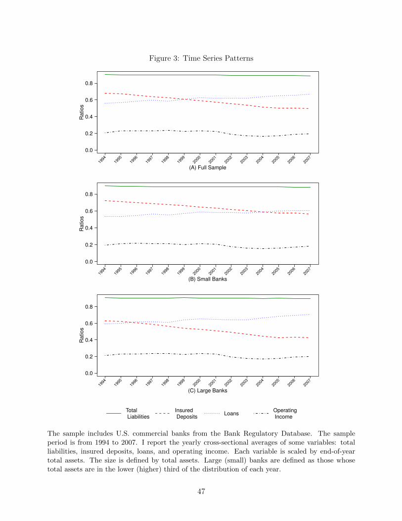
Figure 3: Time Series Patterns

(A) Full Sample

Ratios

1994

1995

1996

1997

1998

1999

2000

2001

2002

2003

2004

2005

2006

2007

0.0

0.2

0.4

0.6

0.8

(B) Small Banks

Ratios

1994

1995

1996

1997

1998

1999

2000

2001

2002

2003

2004

2005

2006

2007

0.0

0.2

0.4

0.6

0.8

(C) Large Banks

Ratios

1994

1995

1996

1997

1998

1999

2000

2001

2002

2003

2004

2005

2006

2007

0.0

0.2

0.4

0.6

0.8

Total Liabilities

Insured Deposits

LoansOperating Income

The sample includes U.S. commercial banks from the Bank Regulatory Database. The sampleperiod is from 1994 to 2007. I report the yearly cross-sectional averages of some variables: totalliabilities, insured deposits, loans, and operating income. Each variable is scaled by end-of-yeartotal assets. The size is defined by total assets. Large (small) banks are defined as those whosetotal assets are in the lower (higher) third of the distribution of each year.

47

Figure 4: Dynamics of Banks nearing Bankruptcy

1 2 3 4 5

0.8

0.9

1.0

1.1

1.2

(A)

Loans

1 2 3 4 5

0.9

01.0

01.1

0

(B)

Debt

1 2 3 4 5

1.0

01.0

21.0

41.0

6

(C)

Inte

rest R

ate

(%

)

Original Belief 1% Higher Belief

First, I simulate the model twice and generate 10,000 hypothetical banks in each iteration: onewith the estimated value for the bailout belief η (blue solid line) as in Table III, and the other with1% higher than η (red dotted line). Then, the simulated banks are ranked by their distance frombankruptcy, defined by cash balance plus remaining loans after fire-sales if necessary. Next, I splitthe simulated banks into five groups depending on distance from bankruptcy. Banks in the first(fifth) quintile are the closest to (farthest from) bankruptcy. Last, the averages of the variables arecomputed for each quintile.

48

Figure 5: Comparative Statics Using Reserve Requirements

0.00 0.05 0.10 0.15 0.20

0.1

50

.17

0.1

90

.21

(A)

Lo

an

s

0.00 0.05 0.10 0.15 0.20

0.3

20

.33

0.3

40

.35

(B)

De

bt

0.00 0.05 0.10 0.15 0.20

1.0

10

1.0

15

1.0

20

1.0

25

1.0

30

(C)

Inte

rest

Ra

te (

%)

0.00 0.05 0.10 0.15 0.20

0.7

00

.75

0.8

0

(D)

Eq

uity V

alu

e

0.00 0.05 0.10 0.15 0.20

0.0

60

.08

0.1

00

.12

0.1

4

(E)

Ba

nkru

ptc

y F

req

ue

ncy

I simulate the model 20 times while varying the reserve requirement ratio α from 0% to 20%,holding the rest of the parameters fixed at the levels in Table III. For each iteration, I generate10,000 hypothetical banks and compute the averages of some variables. The plots are smoothedusing the spline method.

49

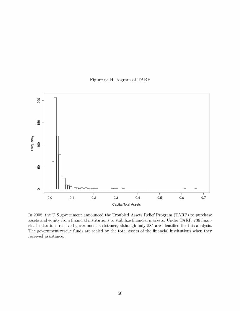
Figure 6: Histogram of TARP

Capital/Total Assets

Fre

quency

0.0 0.1 0.2 0.3 0.4 0.5 0.6 0.7

050

100

150

200

In 2008, the U.S government announced the Troubled Assets Relief Program (TARP) to purchaseassets and equity from financial institutions to stabilize financial markets. Under TARP, 736 finan-cial institutions received government assistance, although only 585 are identified for this analysis.The government rescue funds are scaled by the total assets of the financial institutions when theyreceived assistance.

50