Embed Size (px)
Citation preview
BACTERIAL FORAGING ALGORITHM BASED TUNING OF ON-LOAD TAP
CHANGING TRANSFORMER FOR VOLTAGE REGULATION IN POWER
TRANSMISSION NETWORK
BY
BUKHARI TANKO RABIU
DEPARTMENT OF ELECTRICAL AND COMPUTER ENGINEERING,
FACULTY OF ENGINEERING
AHMADU BELLO UNIVERSITY ZARIA, NIGERIA
AUGUST, 2017

BACTERIAL FORAGING ALGORITHM BASED TUNING OF ON-LOAD TAP
CHANGING TRANSFORMER FOR VOLTAGE REGULATION IN POWER
TRANSMISSION NETWORK
By
Bukhari Tanko RABIU, B.Eng. ATBU Bauchi, 2009
P13EGEE8031
A DISSERTATION SUBMITTED TO THE SCHOOL OF POSTGRADUATE
STUDIES, AHMADU BELLO UNIVERSITY ZARIA, IN PARTIAL FULFILMENT
OF THE REQUIREMENTS FOR THE
AWARD OF MASTER OF SCIENCE (M.Sc.) DEGREE IN POWER SYSTEMS
ENGINEERING
DEPARTMENT OF ELECTRICAL AND COMPUTER ENGINEERING,
FACULTY OF ENGINEERING,
AHMADU BELLO UNIVERSITY ZARIA
NIGERIA
AUGUST, 2017
i
DECLARATION
I, Bukhari Tanko RABIU hereby declare that the work in this dissertation entitled
“Bacterial Foraging Algorithm Based Tuning of On-load Tap Changing Transformer
for Voltage Regulation in Power Transmission Networks” has been carried out by me
under the supervision of Dr Yusuf Jibril and Prof. Boyi Jimoh as part of the requirement
for the award of Degree of Master of Science (M.Sc) in Power Systems Engineering in
the Department of Electrical and Computer Engineering, Ahmadu Bello University
Zaria. The information derived from literature has been duly acknowledged in the text
and a list of references provided. No part of this dissertation was previously presented
for another degree or diploma at this or any other institution to the best of my
knowledge.
Bukhari Tanko RABIU _____________________ ___________________
Signature Date
ii
CERTIFICATION
This Dissertation entitled “Bacterial Foraging Algorithm Based Tuning of On-Load Tap
Changing Transformer for Voltage Regulation in Power Transmission Network” by
Bukhari Tanko RABIU meets the regulations governing the award of Degree of Master
of Science (MSc) in Power Systems Engineering of the Ahmadu Bello University, and
is approved for its contribution to knowledge and literary presentation.
Dr Y. Jibril ________________ ________________
(Chairman, Supervisory Committee) Signature Date
Prof. Boyi Jimoh _________________ _______________
(Member, Supervisory Committee) Signature Date
Dr Y. Jibril ________________ ________________
(Head of Department) Signature Date
Prof. S. Z. Abubakar ________________ ________________
(Dean, School of Postgraduate Studies) Signature Date

iii
DEDICATION
This dissertation is dedicated to Almighty Allah; the Most Beneficient, the Most
Gracious and Most Merciful. Also, to the memory of my late father Alhaji Rabiu Tanko
and to my mother Hajiya Saadatu Isiyaku.

iv
ACKNOWLEDGEMENTS
I am indeed grateful to Almighty Allah for His Infinite Blessings and Guidance towards
the successful completion of this work.
I wish to express my utmost gratitude to my supervisor and also the chairman of my
supervisory committee, Dr Y. Jibril for his time, immense contributions and valuable
guidance towards the success of this work. Indeed, the completion of this work could
not have been possible without your consistent participation and assistance. I am proud
to have you as my supervisor. You helped me a lot in providing valuable suggestions to
the solution of the problems. Thank you very much sir. My thanks also go to my co-
supervisor Prof. Boyi Jimoh for his valuable input and constant encouragement
throughout the stages of the work. I really appreciate the training I received from you.
I acknowledge and appreciate the contributions of all the lecturers of Electrical and
Computer Engineering Department, Ahmadu Bello University Zaria, namely: Prof. B.
G. Bajoga, Prof. U.O Aliyu, Prof. M.B Muazu, Dr A. M. S. Tekanyi, Dr S. M. Sani, Dr
T.H. Sikiru, Dr S. Man-Yahaya, Dr. I. J. Umoh, Dr. K.A. Abu-Bilal, Dr A.D. Usman,
Dr G. A. Olarinoye, Engr. M. J. Mu’azu, Engr. A. I. Abdullahi, Engr Olaniyan
Abdurrahman, Engr Tijjani Ahmed Salahuddeen and those whose names could not be
mentioned. My sincere appreciation also goes to mallam Abdullahi Tukur for his
administrative support towards the completion of this work.
My deepest appreciation goes to all my colleagues in Power System Engineering M.Sc.
class of 2013, Engr. S.M. Aminu, Engr. Imamuddeen Kabir, Engr. Bashir Umar
Charanchi, Engr. Umar Musa, Engr. Lawal Idogwu, Engr. Magaji Muhammad
Batagarawa, Engr. Murtala Mahmud, Engr. Sale Yakubu Gelta, Engr. Musa
Muhammad, Engr. Soliu Abdollahi (Alfa), Engr. Ekpa Dickson, Engr. Yusuf
Habeebullah and Engr. Muhammad Dudu Usman. Furthermore, my appreciation and

v
thanks goes to all members of M.Sc. class of 2013 in Control, Telecommunication,
Computer and Electronic Engineering options. I am indeed grateful to you all; your
handsome reward is with God.
Above all, I am really indebted to my wife, Hajiya Badiya Adamu for her endless love,
support and understanding towards the successful compilation of this work. Thank you
very much. My gratitude also goes to my children, Rabiu Bukhari Rabiu and Hauwau
Bukhari Rabiu, may Allah in his infinite mercy continue to shower his blessings in your
endeavor.
Finally, to my sisters, Hajiya Hadiza Ismaila Ahmed, Hajiya Hauwa Ismaila Rufai,
Malama Ramatu Rabiu Tanko and to my brothers Yusuf Ismaila Ahmed, Isiyaku Rabiu
Tanko and Sulaiman Rabiu Tanko whose love, prayers and elderly advices have kept
me strong and sound all through my life.
Bukhari Tanko RABIU
August, 2017
vi
ABSTRACT
The control of voltage level has been identified as one of the most important operational
needs for efficient and reliable operation of power system equipment. Due to the fact
that both the utility and customer equipment are designed to operate at certain voltage
ratings. Prolonged operation of the equipment at voltages outside the allowable range
could adversely affect their performance and may cause forced outages. Therefore,
voltage at terminals of all equipment in the system has to be kept within acceptable
limits. This dissertation presents the use of Bacterial Foraging Algorithm (BFA) based
tuning of on-load tap changer (OLTC) also known as under load tap changer (ULTC)
transformer for voltage regulation in power transmission network with the intent of
minimizing bus voltage deviation and reduction of transformer tap changing operation.
A standard IEEE C57.131 2012 requirements for tap-changer control (0.85-1.15p.u)
was adopted for this work and the simulation was carried out in MATLAB 2016
platform using power system analysis toolbox (PSAT), the results obtained when
applied on the standard IEEE 14-bus test network, the BFA has demonstrated its
superiority over the conventional method and the ABC algorithm in terms of reduction
in Bus voltage deviation by 0.25% and 0.12% and reduction in transformer taps
changing operation by 0.6% and 0.3% respectively. When applied on the Practical 32-
bus Nigerian power system network, the BFA has also shown a superiority over the
conventional method and the ABC algorithm in all parameters used, with 4.31%, 0.22%
and 0.48% reduction in computational time, bus voltage deviation and transformer tap
changing operations respectively.
vii
LIST OF FIGURES
FIGURE PAGE
Figure 2.1: On-load Tap Changer 10
Figure 2.2: Mechanical Tap Changer with Diverter 11
Figure 2.3: Electronically Assisted Tap Changer 12
Figure 2.4: Transformer with Turns Ratio 14
Figure 2.5: Equivalent Circuit for Tap Changing Transformer 15
Figure 2.6: Typical Bus of the Power System 16
Figure 2.7: Standard IEEE-14 Bus Test Network 19
Figure 2.8: Nigerian 32-Bus Power System Network 20
Figure 2.9: Classification of Optimization Algorithms 21
Figure 2.10: Flow Chart of ABC Algorithm 24
Figure 2.11: Flow Chart of BFA Algorithm 30
Figure 3.1: Base Case Power Flow Analysis of Transmission System Network 37
Figure 3.3: Flow Chart for the Implementation of the Proposed Research 39
viii
LIST OF TABLES
PAGE
Table 3.1: Parameters setting for BFA 40
Table 4.1: Standard IEEE 14-Bus Network using Base Case Power Flow Results 43
Table 4.2: Summary of Simulation Results for the 14-Bus Network using Base case and
ABC algorithm 46
Table 4.3: Summary of Simulation Results for the 14-Bus Network using Base case,
ABC and BFA 48
Table 4.4: Nigerian 32-Bus Power System Network Base Case Power Flow Results 49
Table 4.5: Summary of Simulation Results for the 32-Bus Nigerian Network using Base
case, ABC and BFA 52
ix
LIST OF ABBREVIATIONS
AVC Automatic Voltage Control
ABC Artificial Bee Colony Algorithm
AC Alternating Current
AIS Artificial Immune System
BFO Bacterial Foraging Optimization
COA Chaotic Optimization Algorithm
CRO Coral Reef Optimization Algorithm
CS Cuckoo Search Algorithm
DC Direct Current
DE Differential Evolution
DETC De-Energized Tap Changer
EP Evolutionary Programming
ES Evolutionary Strategy
FA Firefly Algorithm
FACTS Flexible Alternating Current Transmission System
GA Genetic Algorithms
GSA Gravitational Search Algorithm
HS Harmony Search Algorithm
HV High Voltage
HVAC High Voltage Alternating Current
HVDC High Voltage Direct Current
ICA Imperialistic Competition Algorithm
IGBT Insulated-Gate Bipolar Transistor
IWD Intelligent Water Drops Algorithm
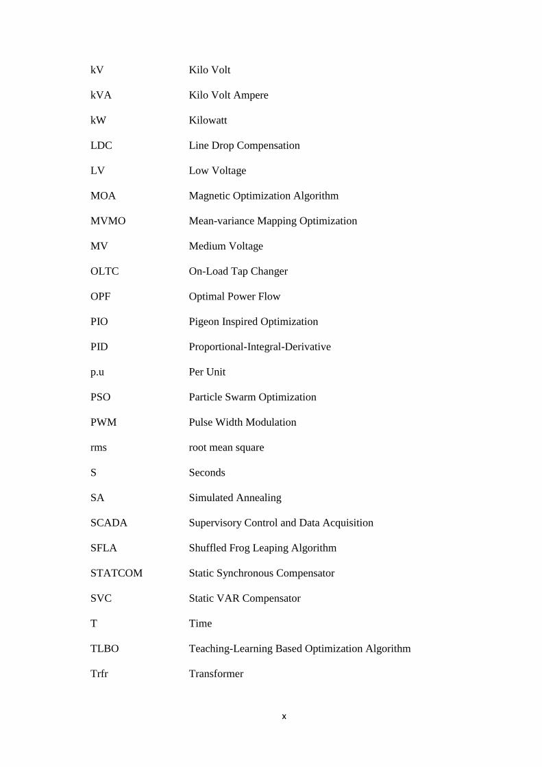
x
kV Kilo Volt
kVA Kilo Volt Ampere
kW Kilowatt
LDC Line Drop Compensation
LV Low Voltage
MOA Magnetic Optimization Algorithm
MVMO Mean-variance Mapping Optimization
MV Medium Voltage
OLTC On-Load Tap Changer
OPF Optimal Power Flow
PIO Pigeon Inspired Optimization
PID Proportional-Integral-Derivative
p.u Per Unit
PSO Particle Swarm Optimization
PWM Pulse Width Modulation
rms root mean square
S Seconds
SA Simulated Annealing
SCADA Supervisory Control and Data Acquisition
SFLA Shuffled Frog Leaping Algorithm
STATCOM Static Synchronous Compensator
SVC Static VAR Compensator
T Time
TLBO Teaching-Learning Based Optimization Algorithm
Trfr Transformer

xi
ULTC Under Load Tap Changer
VAr Volt-Ampere reactive

xii
LIST OF SYMBOLS
1 2and Weighting metrics
tOLTC Total operations of OLTC for hour t
P Active power
Q Reactive power
tapTr,min Minimum Tap position of transformer Tr
tapTr,max Maximum Tap position of transformer Tr
minv Minimum voltage magnitude of the buses
maxv Maximum voltage magnitude of the buses
v Voltage magnitude of the buses
maxs Maximum flow limit through the transmission line
s Flow through the transmission line
i Current flow through the cables, lines and transformers
maxi Maximum current flow through the cables, lines and
transformers
xiii
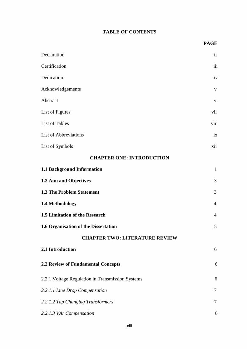
TABLE OF CONTENTS
PAGE
Declaration ii
Certification iii
Dedication iv
Acknowledgements v
Abstract vi
List of Figures vii
List of Tables viii
List of Abbreviations ix
List of Symbols xii
CHAPTER ONE: INTRODUCTION
1.1 Background Information 1
1.2 Aim and Objectives 3
1.3 The Problem Statement 3
1.4 Methodology 4
1.5 Limitation of the Research 4
1.6 Organisation of the Dissertation 5
CHAPTER TWO: LITERATURE REVIEW
2.1 Introduction 6
2.2 Review of Fundamental Concepts 6
2.2.1 Voltage Regulation in Transmission Systems 6
2.2.1.1 Line Drop Compensation 7
2.2.1.2 Tap Changing Transformers 7
2.2.1.3 VAr Compensation 8
xiv
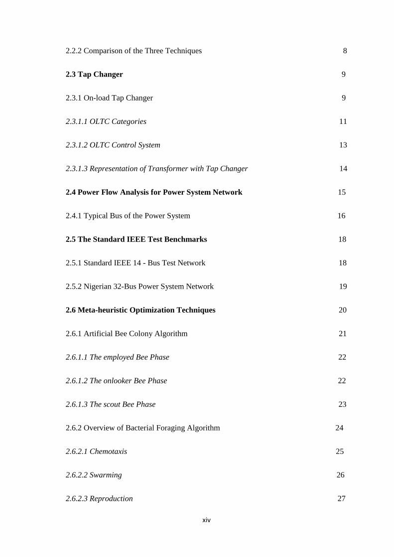
2.2.2 Comparison of the Three Techniques 8
2.3 Tap Changer 9
2.3.1 On-load Tap Changer 9
2.3.1.1 OLTC Categories 11
2.3.1.2 OLTC Control System 13
2.3.1.3 Representation of Transformer with Tap Changer 14
2.4 Power Flow Analysis for Power System Network 15
2.4.1 Typical Bus of the Power System 16
2.5 The Standard IEEE Test Benchmarks 18
2.5.1 Standard IEEE 14 - Bus Test Network 18
2.5.2 Nigerian 32-Bus Power System Network 19
2.6 Meta-heuristic Optimization Techniques 20
2.6.1 Artificial Bee Colony Algorithm 21
2.6.1.1 The employed Bee Phase 22
2.6.1.2 The onlooker Bee Phase 22
2.6.1.3 The scout Bee Phase 23
2.6.2 Overview of Bacterial Foraging Algorithm 24
2.6.2.1 Chemotaxis 25
2.6.2.2 Swarming 26
2.6.2.3 Reproduction 27
xv
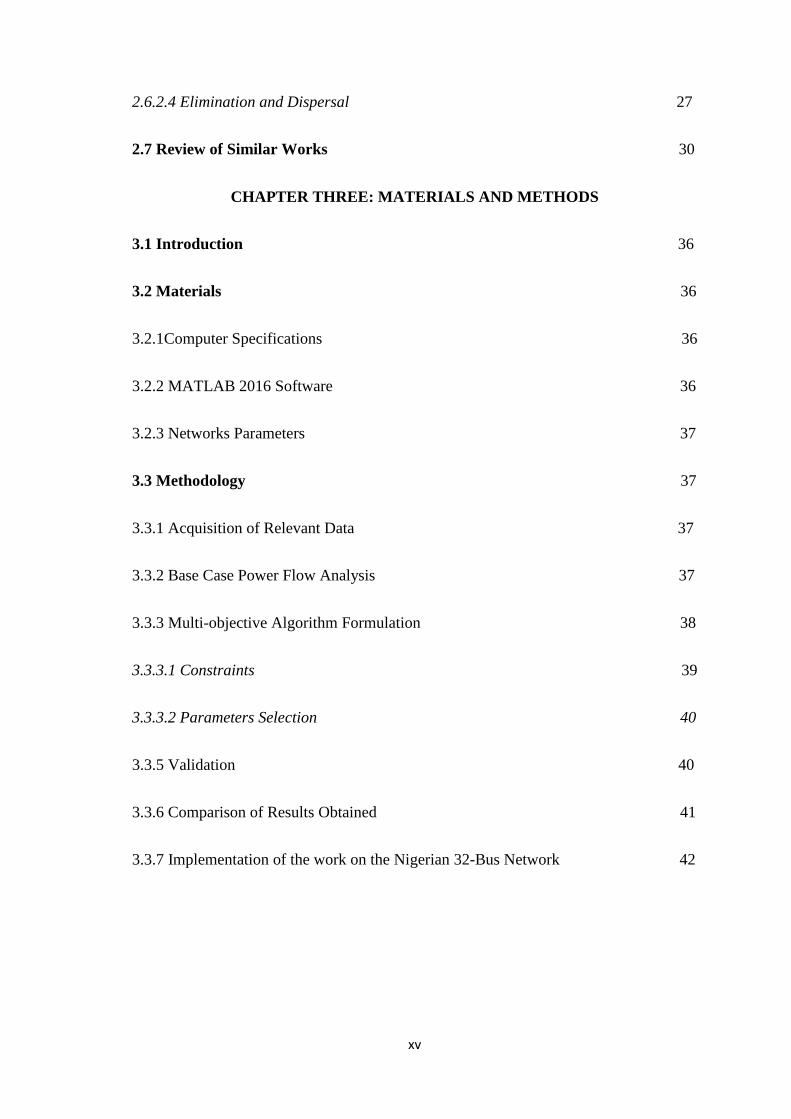
2.6.2.4 Elimination and Dispersal 27
2.7 Review of Similar Works 30
CHAPTER THREE: MATERIALS AND METHODS
3.1 Introduction 36
3.2 Materials 36
3.2.1Computer Specifications 36
3.2.2 MATLAB 2016 Software 36
3.2.3 Networks Parameters 37
3.3 Methodology 37
3.3.1 Acquisition of Relevant Data 37
3.3.2 Base Case Power Flow Analysis 37
3.3.3 Multi-objective Algorithm Formulation 38
3.3.3.1 Constraints 39
3.3.3.2 Parameters Selection 40
3.3.5 Validation 40
3.3.6 Comparison of Results Obtained 41
3.3.7 Implementation of the work on the Nigerian 32-Bus Network 42
xvi
CHAPTER FOUR: RESULTS AND DISCUSSIONS
4.1 Introduction 43
4.2 The Standard IEEE 14-Bus Power System Network 44
4.2.1 Network Bus Voltage Deviation using Base case and ABC Algorithm 45
4.2.2 Performance Comparison for Transformer Tap Changing Operation Reduction
using Base case and ABC Algorithm 47
4.2.3 Network Bus Voltage Deviation using Base case, ABC Algorithm and BFA 47
4.2.4 Performance Comparison for Transformer Tap Changing Operation Reduction
using Base case, ABC Algorithm and BFA 48
4.3 The Nigerian 32-Bus Power System Network 49
4.3.1 Network Bus Voltage Deviation using Base case, ABC Algorithm and BFA 50
4.3.2 Performance Comparison for Transformer Tap Changing Operation Reduction
using Base case and ABC Algorithm 51
CHAPTER FIVE: CONCLUSION AND RECOMMENDATIONS
5.1 Summary 54
5.2 Conclusion 54
5.3 Significant Contributions 54
5.4 Recommendations for Further Works 55
REFERENCES 56
APPENDICES

xvii
Appendix A1: Bus Data for Standard IEEE-14 Bus Network 60
Appendix A2: Line Data for Standard IEEE-14 Bus Network 60
Appendix A4: Bus Data of the Nigerian 32-Bus Power System Network 61
Appendix A5: Line Data of the Nigerian 32-Bus Power System Network 62
Appendix B1: m-File for ABC and BFA 64
1
CHAPTER ONE
INTRODUCTION
1.1 Background Information
Power system engineering forms a vast and major portion of electrical engineering
studies. It is mainly concerned with the generation of electrical power and its
transmission from sending end to the receiving end as per consumer requirements,
incurring minimum amount of losses. Power at the transmission level is often subjected
to changes due to disturbances incurred within the length of the grid, for this reason the
term power system stability is of utmost importance in this field (Acha et al., 2011).
The control of voltage level has been identified as one of the most important operational
needs for efficient and reliable operation of power systems equipment, due to the fact
that both the utility and customer equipment are designed to operate at a certain voltage
rating (Salem, 2007). In general, there are two ways of regulating the voltage; by
injection or absorption of reactive power from the system using Flexible Alternating
Current Transmission System (FACTS) devices and by direct control of voltage
amplitude using On Load Tap Changer (OLTC) (Mohammed, 2011).
A tap changer is a connection point selection mechanism along a power transformer
winding that allows a variable number of turns to be selected in discrete steps. A
transformer with a variable turn’s ratio is required to enable stepped voltage regulation
of the output. The tap selection may be made via an automatic or manual tap changer
mechanism. Generally, tap changers are classified into two types: off-circuit also known
as De-Energised Tap Changer (DETC) and on-Load Tap Changer (OLTC),
(Vigneshwaran and Yuvaraja, 2015).
2
OLTC is considered in this work and is generally classified as mechanically and
electronically assisted as well as solid state tap changers. Earlier, mechanical type and
solid state on-load tap changers were in practice, but they had considerable limitations
such as arcing, high maintenance cost and slow reaction times.
To overcome the above mentioned limitations, a meta-heuristic optimization technique
known as Bacterial Foraging Algorithm (BFA) was employed; which was developed by
Kevin Passino, (2002). It was inspired by the foraging behaviour of Escherichia Coli
(E.Coli) bacteria found in the human intestines (Xing and Gao, 2014). The algorithm
was formulated on the basis of four principal processes: Chemotaxis, Swarming,
Reproduction and Elimination-dispersal (Boussaid et al., 2013). The rationale behind
selecting BFA is that it is not largely affected by the size and non-linearity of the
problem; also it converges to the optimal solution in many problems where most
analytical methods have failed to converge. The algorithm also has advantages such as
global convergence, high exploration capacity and can handle more number of objective
functions when compared to other evolutionary algorithms. However, this work seeks to
use the algorithm for optimal tuning of OLTC in reduction of transformer tap changing
operations as well as bus voltage deviation in power transmission networks.
1.2 Problem Statement
The control of voltage has been identified as one of the most important operational
requirements for efficient and reliable operation of power systems equipment, due to the
fact that both the utility and customer equipment are designed to operate at some certain
acceptable voltage ratings (Salem, 2007). Prolonged operation of the equipment at
voltages outside the allowable range could adversely affect their performance, resulting
in forced outages. Therefore, voltage at each terminals of all equipment in the system
3
has to be kept within acceptable limits of (0.85 - 1.15p.u) as defined by IEEE standard
C57.131 2012 OLTC control requirement (Hashemi, 2011).
1.3 Aim and Objectives
The aim of this research is to apply Bacterial Foraging Algorithm for tuning of on-load
tap changing transformer for voltage regulation in power transmission network.
The objectives are:
i. Application of BFA for tuning of OLTC transformer in standard IEEE 14-Bus
network.
ii. Validation of the results obtained in item (i) using BFA by comparison with
those of the work of Mostafa Abdollah et al., (2013)
iii. Implementation of the proposed approach on the Nigerian 32-Bus Power system
network.
1.4 Research Methodology
The objectives as outlined in this research were actualized in line with the following
procedures:
i. Acquire relevant networks data (line data, bus data, network base voltage, etc.)
from TCN Mando Kaduna;
ii. Perform network base-case power flow analysis using Newton Raphson
technique;
iii. Adoption of Bacterial Foraging Algorithm on the standard IEEE-14 Bus
Network.
iv. Formulation of multi-objective functions for standard IEEE 14-bus network
comprising of bus voltage deviation and transformer tap changing operation to
be used in both ABC and BFA;
4
v. Application of BFA with the formulated multi-objective functions for reduction
of bus voltage deviation and transformer tap changing operation.
vi. Comparison between the results obtained for ABC and BFA in both graphical
and tabular forms.
vii. Implementation of the proposed approach by repeating the fourth and fifth
procedures on the Nigerian 32-bus power system network using graphical and
tabular form representation.
1.5 Research limitation
Although one of the objectives of the research was to solve the problem of voltage
instability associated with the Nigerian 32 bus power system network, but after the
application of BFA on OLTC the results obtained are still not within those defined by
the standard, as some of the voltages of the buses are still not within the limits.
1.6 Organisation of the Dissertation
Chapter one presents the general introduction of the dissertation while chapter two
presents the fundamental concepts that include all relevant assumptions, theories and
modelling equations needed for the actualization of the research and a comprehensive
review of similar works carried out. Chapter three presents an elaborate procedure for
the actualization of the research, which include all the materials and the methodology
adopted. The results obtained from the application of the theoretical and modelling
concepts presented in the two previous chapters and their discussions are presented in
chapter four. Chapter five covers the conclusion, recommendation and possible areas of
further work. Finally, references of the works used and appendices are presented.
5
CHAPTER TWO
LITERATURE REVIEW
2.1 Introduction
The literature review comprises of the overview of fundamental concepts as well as the
review of similar works. In the review of fundamental concepts, most of the pertinent
works and the fundamental theories that are used for the success of this research are
reviewed, after which review of similar works followed.
2.2 Review of Fundamental Concepts
In this subsection, concepts that are fundamental and pertinent to the understanding of
OLTC and its control are reviewed.
2.2.1 Voltage Regulation in Transmission systems
The voltage control problem can be defined as the assurance of maintaining electric
power quality at all levels (Fusco and Russo, 2007). Disturbances like over-voltage,
under-voltage, voltage unbalance, and voltage harmonic distortion affect the power
quality which causes serious problems. The two approaches for voltage control are the
off-line control that depends on dispatch schedule ahead of time as a forecast of the
voltage changes; and the on-line (automatic) that depends on real-time measurements of
voltage. Moreover, the active network management of a power system may be
categorized into coordinated control, semi-coordinated or decentralized control
strategies. Centralized or coordinated control strategy provides voltage control from the
substation towards the rest of the network. On the other hand, semi-coordinated and
decentralized control strategies must be able to control each unit locally in an active
manner while coordinating it with a limited number of other network devices (Hashim
et al., 2012).
In a centralized or co-ordinated voltage control scheme, several techniques are
implemented including distribution management system control, distribution system
6
components (like VAr compensator and step voltage regulator), intelligent centralized
method like meta-heuristic algorithm as well as multi-agent system (Viawan, 2008).
The techniques implemented in the decentralized voltage control scheme are
summarized into reactive power compensation, power factor voltage control, on-load
tap changer, generation curtailment and intelligent decentralized systems. By reviewing
the research conducted on voltage regulation at both transmission and distribution
systems, it is concluded that tap-changing transformers, VAR compensators and line
drop compensation are the techniques that are mostly used for voltage control.
2.2.1.1 Line Drop Compensation
Line Drop Compensation (LDC) is a traditional method of calculating the voltage drop
along each line, hence calculating the voltages at each terminal accordingly. This
method can be applied once by setting the voltage according to the calculated voltages
at the consumer, or using a tap changer. This method doesn’t provide accurate results
due to several reasons. For instance, the addition of distributed generation makes the
line drop calculations not accurate.
The voltage drops on a line between the source bus-bar and the load is calculated by
Automatic Voltage Control (AVC) relay using the input current and the impedance
value of the line (Dai, 2012). The relay adjusts the control parameter to increase or
compensate the source bus-bar voltage by an amount equal to the calculated voltage
drop. The impedance of a line might not be accurate since there might be several
branches extending from one feeder like in tree network arrangement. In addition, the
AVC relay can have one feeder resistance (R) and reactance (X) setting although most
substations have multiple feeders. In order to resolve these shortcomings, the R and X
settings on the LDC is based on a hypothetical composite feeder model that has to cater
for the worst combination of demands on each of the feeders (Dai, 2012).
7
2.2.1.2 Tap-changing transformers
Tap-changing transformer technique uses an off-line or on-line tap changer to regulate
the voltage to a reference level. The tap changer can be placed at the primary or
secondary side of the transformer. It varies the number of turns in a transformer by
adjusting the turns’ ratio in order to achieve the required voltage at the secondary side
of the transformer (Viawan, 2008).
2.2.1.3 VAR Compensation
VAR compensation or reactive power control is a technique to regulate the voltage
using reactive elements or FACTS devices such as static synchronous compensator
(STATCOM), static VAR compensator (SVC), static synchronous series compensator
(SSSC) and unified power flow controller (UPFC) or switched fixed
capacitors/inductors e.g. shunt capacitors (Romero, 2010). The method is based on
measuring the line voltage, comparing it with a reference level and connecting
compensators (reactive or capacitive) to regulate the voltage. VAr compensation has
considerable limitations; the latest technique considers the use of VAr compensation
with DG.
2.2.2 Comparison of the three Techniques
The three techniques as mentioned earlier play an important role in the regulation of
voltage. However, several problems arise at transmission networks such as voltage
instability, line drops, etc. All the three techniques depend on forecasted voltages which
are not real and accurate. In addition, they mostly depend on power flow analysis which
can resolve static equations and cannot provide dynamic analysis.
The line drop compensation is simple; however, it doesn’t provide accurate results due
to the change in loads and the addition of feeders in the network. The VAR
compensation technique requires several capacitors at the feeders. The control in the
8
tap-changing transformer is more complex, even though OLTC can provide better
values than line drop and VAr compensation. However, the control still is based on
forecasted and not real loads since the voltages at the end customers cannot be
measured in the traditional distribution networks. The evolution towards advanced
metering infrastructure and the use of smart meters to measure the voltages in real time
plays an important role in the enhancement of voltage control techniques. Hence, the
OLTC became more attractive and promising solution for much more accurate, faster
and simple dynamic voltage control at sub-transmission and distribution systems (Dai,
2012).
2.3 Tap Changer
A tap changer is a selection tool in power transformer windings that permits a variable
number of turns to be selected in discrete steps. A transformer with a variable primary
to secondary turns’ ratio is formed, allowing stepped voltage regulation of the output.
The tap selection may be made via an automatic or manual tap changer mechanism. The
mechanism of tap-changing can be made on-load or off-load. If there is no load
connected to the transformer, the tool is called off-load, DETC or no-load tap changer.
However, the tap-changer that works during load is called under-load tap changer or on-
load tap changer (Faiz and Siahkolah, 2006).
2.3.1 On-Load Tap Changer
The OLTC of power transformers has been proven to have a fundamental importance as
a voltage regulating mechanism. The switching principle is that the turn ratio of a
transformer can be changed by adding to or subtracting turns on either the primary, or
the secondary windings. As indicated by its name, changing the tap position is possible
only when the power transformer is carrying load. With transformers equipped with
OLTC the voltage can be controlled within acceptable range. The OLTC can be located
9
at the primary or the secondary side of the transformer, although in the most case the
variable tap is on the HV side. One reason for this choice is that the current on the HV
side is lower, and consequently the commutation is easier. In addition, the more turns
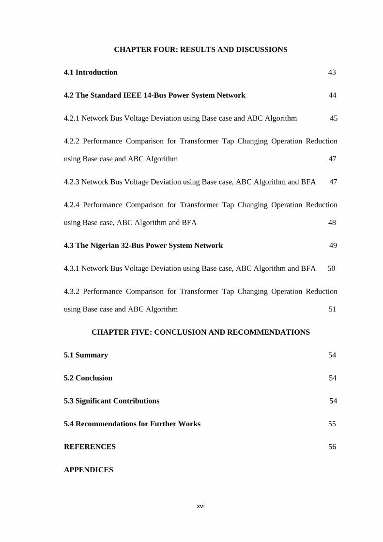
that are available in this side enable a more accurate voltage regulation. Figure 2.1
shows the diagram of OLTC transformer (Viawan, 2008).
Figure 2.1: On-load Tap Changer (Romero, 2010)
One important constraint is the finite number of tap positions existing in the device. A
typical OLTC has 16 lower taps, 16 upper taps and one neutral tap for a total of 33 taps.
Some OLTCs have multiple neutral taps or may have only 8 lower and 8 upper taps.
Thus, the voltage regulation is restricted to a range defined by the lower and the upper
voltage limit ranging from 0.85 p.u to 1.15p.u (Gohil and Verma, 2016).
The OLTC have to be more frequently regulated in order to maintain the voltage
profiles between the acceptable ranges. This leads to an increased operation and
maintenance cost of the transformers. Consequently, the limitation of OLTC operations
is included in the proposed approach (Viawan, 2008).
2.3.1.1 OLTC Categories
OLTCs may be classified into three different categories
i. Mechanical tap changer
ii. Electronically-assisted tap changer
10
iii. Solid-state tap changer
A mechanical tap changer makes physically the new tap connection before releasing the
old one, using multiple tap selector switches. It avoids creating high circulating currents
by using a diverter switch to temporarily place large diverter impedance in series with
the short-circuited turns as shown in Figure 2.2a. This technique overcomes the
problems with open or short circuit taps. In a resistance type tap changer, the
changeover must be made rapidly to avoid overheating of the diverter.
A reactance type tap changer uses a dedicated preventive auto-transformer winding to
function as the diverter impedance. A reactance type tap changer is usually designed to
sustain off-tap loading indefinitely as shown in Figure 2.2b (Romero, 2010).
(a)Resistance Type (b) Reactance Type
Figure 2.2: Mechanical Tap Changer with Diverter (Romero. 2010)
The mechanical tap-changers have many disadvantages like arcing in the diverter
switches during tap changing process, high maintenance cost, slow taps changing speed
and high losses in the tap change (Nadeem et al., 2013). The arc in the contacts of
diverter switches during the tap-changing process is an essential problem in the
mechanical under-load tap changer (Faiz and Siahkolah, 2011).
11
Electronically-assisted tap changers are developed to resolve this issue by reducing the
arc with more controllability of the switches. One type of such tap changers uses
thyristor to take the on-load current while the main contacts change over from one tap to
the other (Martinez et al., 2013).
A sample connection between contacts A and B of a certain tap is shown in Figure 2.3
below:
Figure 2.3: Electronically Assisted Tap Changer (Ram et al., 2015)
An OLTC with electronically-assisted tap changer is designed in (Ram et al., 2015) and
a lab setup illustrating its application is presented in (Romero, 2010). The use of hybrid
configuration of mechanical and bidirectional electronic switches that switch between
no-load and on-load situations was proposed by (Martinez et al., 2013).
Solid-state tap changer uses bidirectional solid state relays (SSR) to switch the
transformer winding taps and to pass the load current in the steady state. The design and
implementation of SSR can be made from several configurations of power electronic
devices including Insulated-Gate Bipolar transistor or gate turn-off thyristor (Romero,
2010). The performance comparison of mechanical and electronic tap-changers
indicated that the following differences are required in goals and responsibilities of
controllers of these two categories of tap-changers (Faiz and Siahkolah, 2011). A
reduction of the tap-changing frequency in the controller of mechanical tap-changer is
one of the design objectives, while this is not the case in an electronic tap-changer. In a

12
mechanical tap-changers controller, taps must be changed step-by-step, while there is no
such limitation in an electronic tap-changer (Faiz and Siahkolah, 2011).
A complicated arrangement of taps and switches in the control system of an electronic
tap-changer makes it necessary to have a look-up table for storing the position of each
switch which corresponds to each of the output states. Such a look-up table is not
required in mechanical tap-changer. The tap-changing process is very quick with an
SSCT, so there is a need to use an algorithm for quick and accurate detection of the
amplitude and phase of the sinusoidal variables such as primary and secondary voltages
and load current. In contrast, the tap-changing process is much slower in a mechanical
tap-changer, so averaging methods over several cycles to determine the rms voltage and
current are sufficient. In electronic tap-changer controller, it is necessary to detect the
zero-crossing of the load current in order to have soft switching of the tap-changer
switches. In a mechanical tap-changer, the tap-changing process is slower, so soft
switching cannot be realized (Faiz and Siahkolah, 2011).
2.3.1.2 OLTC Control System
Whenever the electrical supply network voltage is less than the optimal value, there is a
chance of nuisance tripping of voltage sensitive equipment and devices. The OLTC is
therefore very necessary in order to maintain a constant bus voltage on the Medium
Voltage terminals of a transformer for varying load conditions. It is essential that no tap
change operation is made unless the voltage change on the system is sufficient to justify
the tap change operation, and for this reason it is desirable that operation is not initiated
for a momentary change in voltage. The introduction of an appropriate amount of time
delay reduces the wear and tear on the mechanism and prolongs the life of the OLTC
contacts and the oil in which the arcing takes place (Faiz and Siahkolah, 2011).
13
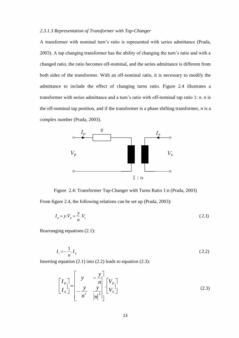
2.3.1.3 Representation of Transformer with Tap-Changer
A transformer with nominal turn’s ratio is represented with series admittance (Prada,
2003). A tap changing transformer has the ability of changing the turn’s ratio and with a
changed ratio, the ratio becomes off-nominal, and the series admittance is different from
both sides of the transformer. With an off-nominal ratio, it is necessary to modify the
admittance to include the effect of changing turns ratio. Figure 2.4 illustrates a
transformer with series admittance and a turn’s ratio with off-nominal tap ratio 1: n. n is
the off-nominal tap position, and if the transformer is a phase shifting transformer, n is a
complex number (Prada, 2003).
Figure 2.4: Transformer Tap-Changer with Turns Ratio 1:n (Prada, 2003)
From figure 2.4, the following relations can be set up (Prada, 2003):
. . ( 2.1)p p s
yI y V V
n
Rearranging equations (2.1):
1. ( 2.2)s pI I
n
Inserting equation (2.1) into (2.2) leads to equation (2.3):
S
P
S
P
V
V
n
y
n
yn
yy
I
I.
2
(2.3)
14
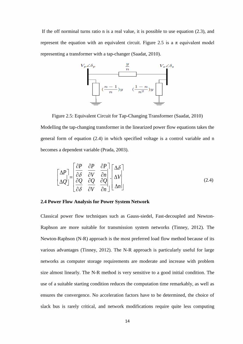
If the off norminal turns ratio n is a real value, it is possible to use equation (2.3), and
represent the equation with an equivalent circuit. Figure 2.5 is a π equivalent model
representing a transformer with a tap-changer (Saadat, 2010).
Figure 2.5: Equivalent Circuit for Tap-Changing Transformer (Saadat, 2010)
Modelling the tap-changing transformer in the linearized power flow equations takes the
general form of equation (2.4) in which specified voltage is a control variable and n
becomes a dependent variable (Prada, 2003).
n
V
n
Q
V
QQn
P
V
PP
Q
P
. (2.4)
2.4 Power Flow Analysis for Power System Network
Classical power flow techniques such as Gauss-siedel, Fast-decoupled and Newton-
Raphson are more suitable for transmission system networks (Tinney, 2012). The
Newton-Raphson (N-R) approach is the most preferred load flow method because of its
various advantages (Tinney, 2012). The N-R approach is particularly useful for large
networks as computer storage requirements are moderate and increase with problem
size almost linearly. The N-R method is very sensitive to a good initial condition. The
use of a suitable starting condition reduces the computation time remarkably, as well as
ensures the convergence. No acceleration factors have to be determined, the choice of
slack bus is rarely critical, and network modifications require quite less computing
15
effort. The N-R method has great generality and flexibility, hence enabling a wide range
of representational requirements to be included easily and efficiently, such as on-load
tap changing and phase-shifting devices, area interchanges, functional loads and remote
voltage control (Tinney, 2012). The N-R load flow is central to many recently
developed methods for the optimisation of power system operation, sensitivity analysis,
system-state estimation, linear-network modelling, security evaluation and transient-
stability analysis, and it is well suited to online computation (Stott, 2009).
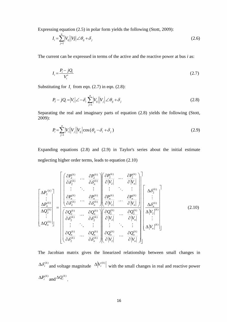
2.4.1 Typical Bus of the Power System
The relationship between real and reactive power in power system network can be
established from Figure 2.6:
iV
1V
2V
nV
1iY
2iY
inY
ioY
iI
Figure 2.6: Typical Bus of the Power System (Stott, 2009)
Power flow equations are formulated in polar form for the n-bus system in terms of bus
admittance matrix Y as follows: (Stott, 2009).
1
(2.5)n
i ij
j
I Y V
Where i, j are to denote thi and thj bus.
16
Expressing equation (2.5) in polar form yields the following (Stott, 2009):
1
(2.6)n
i ij ij j
j
I V Vj
The current can be expressed in terms of the active and the reactive power at bus i as:
(2.7)i ii
i
P jQI
V
Substituting for iI from eqn. (2.7) in eqn. (2.8):
1
(2.8)n
I i i i ij j ij j
j
P jQ V V V
Separating the real and imaginary parts of equation (2.8) yields the following (Stott,
2009):
1
cos ( ) (2.9)n
i i j ij ij i j
j
P V V V
Expanding equations (2.8) and (2.9) in Taylor's series about the initial estimate
neglecting higher order terms, leads to equation (2.10)
)(
)(
2
)(
2
k
n
k
k
n
k
Q
Q
P
P
( ) ( )( ) ( )2 22 2
( ) ( )22
( ) ( ) ( ) ( )
( ) ( )
2 2
(( )( )22
( ) ( )
2 2
( ) ( )
( ) ( )
2
k kk k
k knn
k k k k
n n n n
k k
n n
kkk
n
k k
k k
n n
k k
n
P PP P
V V
P P P P
V V
QQQ
Q Q
( )
2
( )
( )) ( )
22
2
( )
( ) ( )
2
(2.10)
k
k
n
kk
n
k
nk k
n n
n
VQ
V V
V
Q Q
V V
The Jacobian matrix gives the linearized relationship between small changes in
)(k
i and voltage magnitude )(k
iV with the small changes in real and reactive power
)(k
iP and)(k
iQ.
17
1 2
3 4
(2.11)J JP
J JQ V
The diagonal and the off-diagonal elements of 1J are as follows:
1
cos( ) (2.12)n
ik ij ij i j
ji
PVi V Y
sin ( ) (2.13)ii j ij ij i j
j
PV V Y
Similarly, the diagonal and off-diagonal elements of 2 3 4,J J and J. The terms
)(k
iP
and )(k
iQ are the difference between the scheduled and calculated values, known as the
power residuals.
( ) (2.14)k sch k
i i iP P P
( ) ( ) (2.15)k sch k
i i iQ Q Q
Values of the power residuals and the Jacobian matrices, )(k
i and )(k
iV are
calculated from the equation (2.10), to complete the particular iteration and the values
calculated as shown below are used for the next iteration (Stott, 2009).
( 1) ( ) ( ) (2.16)k k k
i i i
( 1) ( ) ( ) (2.17)k k k
i i iV V V
2.5 The Standard IEEE Test Benchmarks
The standard IEEE Test Platforms are made available for researchers in order to have a
common IEEE Standard test beds for uniform comparisons. These test beds are used
both in transmission and distribution systems. Some of the IEEE transmission test
18
networks are 11 bus, 14 bus, 30 bus, 33 bus, 40 bus, 57 bus, 69 bus, 118 bus, 200 bus
and 300 bus etc.
Furthermore, there are 10 Indian bus networks and 33 Turkey networks, 200 England
bus networks, as part of standard test networks (Cai, 2010).
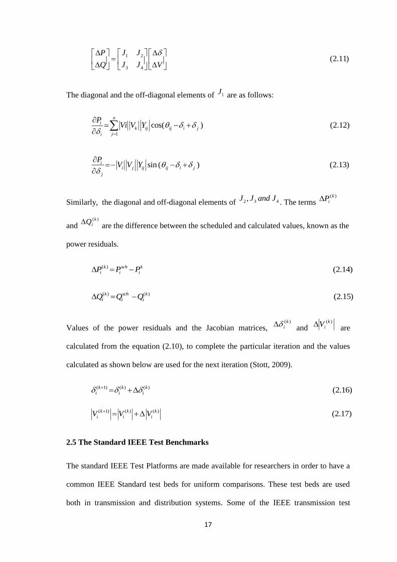
2.5.1 Standard IEEE 14-Bus Test Network
The standard IEEE 14 bus test system will be used to test the proposed BFA method.
Figure 2.7 shows the test system. The system bus and line data are given in Appendix
A1 & A2 respectively. The transformer between bus 4 and 9 is OLTC transformer and it
aims at controlling the voltage at bus 9 (Abdollah et al., 2013).
1
2
3
4
5
6 7 8
9
1011
12
13
14
Figure 2.7: Standard IEEE 14 Bus Test Network (Abdollah et al., 2013)
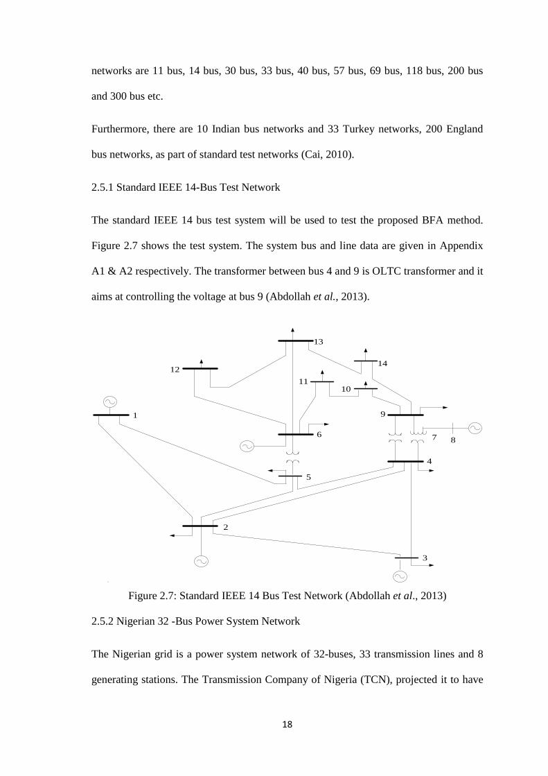
2.5.2 Nigerian 32 -Bus Power System Network
The Nigerian grid is a power system network of 32-buses, 33 transmission lines and 8
generating stations. The Transmission Company of Nigeria (TCN), projected it to have
19
the capacity to deliver about 12,500MW in 2014, has the capacity of delivering
4475.87MW of electricity. Nigeria has a transmission capability of 5,228MW with peak
production of 4,500MW against a peak demand forecast of 10,200MW (Eseosa and
Odiase, 2015).
This shows that if the generation sector is to run at full production, the transmission grid
will not have the capacity to handle the produced power reliably (Eseosa and Odiase,
2015). Figure 2.8 shows the single line diagram of the Nigerian 32-bus power system
network. The Bus data of the Nigerian 32-bus power system network was provided in
Appendix A4 and the Line data was also provided in Appendix A5.
1Kaduna T.S
2KanoT.S
3JosT.S
4GombeT.S
5Kainji G.S
6Jebba G.S7ShiroroG.S
8Jebba T.S
9OsogboT.S10AyedeT.S
11Olorun T.S
12SaketeT.S
13Akangba T.S
14Ikeja West T.S
15Egbin G.S
16Aja T.S
17OmotoshoG.S
18Benin T.S
19Delta G.S
20SapeleG.S
21Onisha T.S
22Okpai T.S
23N / Heaven T.S
24Ajaokuta T.S
25Geregu G.S
26AlaojiT.S
27 AfamT.S
28B / Kebbi T.S
29GanmoT.S
30KatampeT.S
31Aladja T.S
32Alaoji G.S
Figure 2.8: Nigerian 32-Bus Power System Network (Eseosa and Odiase, 2015)
2.6 Meta-heuristic Optimization Techniques
Meta-heuristic optimization techniques represent a group of intelligent algorithms that
make analogy of the natural evolution process based on Darwinian principles or mimic
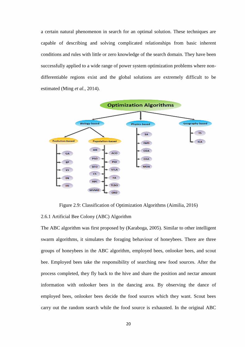
20
a certain natural phenomenon in search for an optimal solution. These techniques are
capable of describing and solving complicated relationships from basic inherent
conditions and rules with little or zero knowledge of the search domain. They have been
successfully applied to a wide range of power system optimization problems where non-
differentiable regions exist and the global solutions are extremely difficult to be
estimated (Ming et al., 2014).
Figure 2.9: Classification of Optimization Algorithms (Aimilia, 2016)
2.6.1 Artificial Bee Colony (ABC) Algorithm
The ABC algorithm was first proposed by (Karaboga, 2005). Similar to other intelligent
swarm algorithms, it simulates the foraging behaviour of honeybees. There are three
groups of honeybees in the ABC algorithm, employed bees, onlooker bees, and scout
bee. Employed bees take the responsibility of searching new food sources. After the
process completed, they fly back to the hive and share the position and nectar amount
information with onlooker bees in the dancing area. By observing the dance of
employed bees, onlooker bees decide the food sources which they want. Scout bees
carry out the random search while the food source is exhausted. In the original ABC
21
algorithm (Karaboga, 2005), the number of food sources is equal to the number of
employed bees. The number of employed bees is equal to number of onlooker bees
simultaneously. In other words, a half of the colony size is employed bees. The process
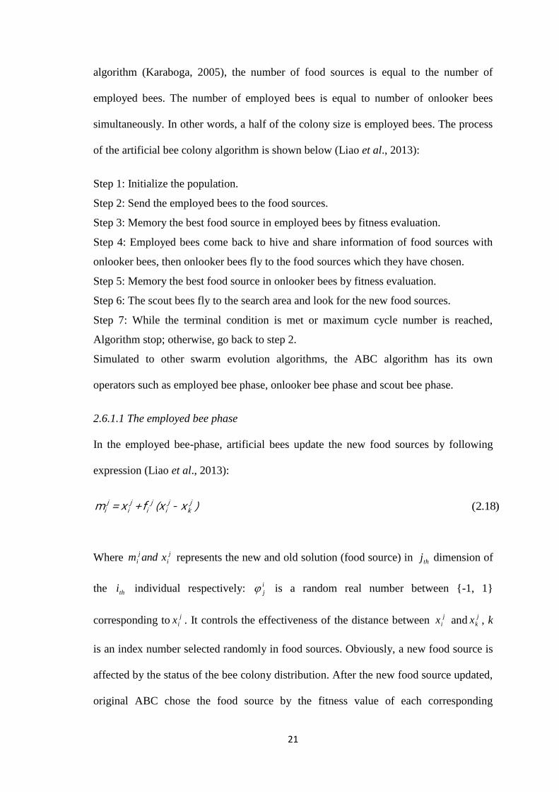
of the artificial bee colony algorithm is shown below (Liao et al., 2013):
Step 1: Initialize the population.
Step 2: Send the employed bees to the food sources.
Step 3: Memory the best food source in employed bees by fitness evaluation.
Step 4: Employed bees come back to hive and share information of food sources with
onlooker bees, then onlooker bees fly to the food sources which they have chosen.
Step 5: Memory the best food source in onlooker bees by fitness evaluation.
Step 6: The scout bees fly to the search area and look for the new food sources.
Step 7: While the terminal condition is met or maximum cycle number is reached,
Algorithm stop; otherwise, go back to step 2.
Simulated to other swarm evolution algorithms, the ABC algorithm has its own
operators such as employed bee phase, onlooker bee phase and scout bee phase.
2.6.1.1 The employed bee phase
In the employed bee-phase, artificial bees update the new food sources by following
expression (Liao et al., 2013):
(2.18)j j j j ji i i i km =x +f (x - x )
Where j
i
j
i xandm represents the new and old solution (food source) in thj dimension of
the thi individual respectively: i
j is a random real number between {-1, 1}
corresponding toj
ix . It controls the effectiveness of the distance between j
ix andj
kx , k
is an index number selected randomly in food sources. Obviously, a new food source is
affected by the status of the bee colony distribution. After the new food source updated,
original ABC chose the food source by the fitness value of each corresponding
22
employed bee. Greedy selection has been applied in the ABC algorithm in order to
determine which food source is better and would be remembered after the employed bee
phase.
2.6.1.2 The onlooker Bee phase
In the onlooker bee phase, employed bees go to a dance area share the nectar amount
information of a food source, and onlooker bees waiting in the hive chose the employed
bees randomly, but probability is related to the nectar amount. In the ABC algorithm,
the nectar amount represents the fitness value of food source. Therefore, the food
sources which have higher nectar amount information are more likely to be chosen after
onlooker bee phase completed (Liao et al., 2013).
2.6.1.3 Scout Bee phase
After onlooker bee phase, a modified bee colony distribution is determined. If one of
these food sources cannot be improved in pre-determined cycle ‘‘limit’’, it will be
replaced by a new one according to following equation (Liao et al., 2013):
(2.19)j j j ji min max minx = x + rand [0,1] (x - x )
Where jxmin and jxmax represent the lower and upper boundary in dimension j,
respectively; rand {0, 1} is the random number between {0, 1}; Scout bee phase in
ABC is applied to abandon the solution which cannot be improved (Liao et al., 2013).
23
Figure 2.10: Flow Chart of ABC Algorithm (Abdollah et al., 2013)
24
2.6.2 Overview of Bacterial Foraging Algorithm (BFA)
It was originally proposed by Kevin Passino in 2002, the algorithm mimics the foraging
behavior of E. Coli bacteria found in the human intestines (Xing and Gao, 2014). The
algorithm is formulated on the basis of four principal processes namely: chemotaxis,
swarming, reproduction and elimination-dispersal (Boussaid et al., 2013).
2.6.2.1 Chemotaxis
Chemotaxis explains the procedure in which the E. Coli bacteria conducts their
movements towards certain chemicals within the surroundings. The bacteria moves in
either of two ways: swimming or tumbling, with the sole purpose of finding nutrient-
rich areas and avoiding toxic environments. Tumbling is the movement of the bacteria
in a haphazard manner (random direction) whereas swimming is the movement in a
specified direction mostly a unit walk in a previous tumble (Kiani et al., 2013). The
movement of the thi bacterium after one step is given by (Xing and Gao, 2014).
)()(),,(),1( iiClkjli ii (2.20)
Where:
),,( lkji is the location of thi bacterium at thj chemotactic, thk reproductive, thl
elimination and dispersal step,
C(i) is the length of unit walk,
(i) is the direction angle of the thj step,
The fitness function of the thi bacterium is determined based on its position and is
represented by (i, j, k, l)j j (Kiani et al., 2013). The direction angle (i) describes the
tumble of the bacteria and is given by (Boussaid et al., 2013):
25
)(i)()(
)(
ii
i
T
(2.21)
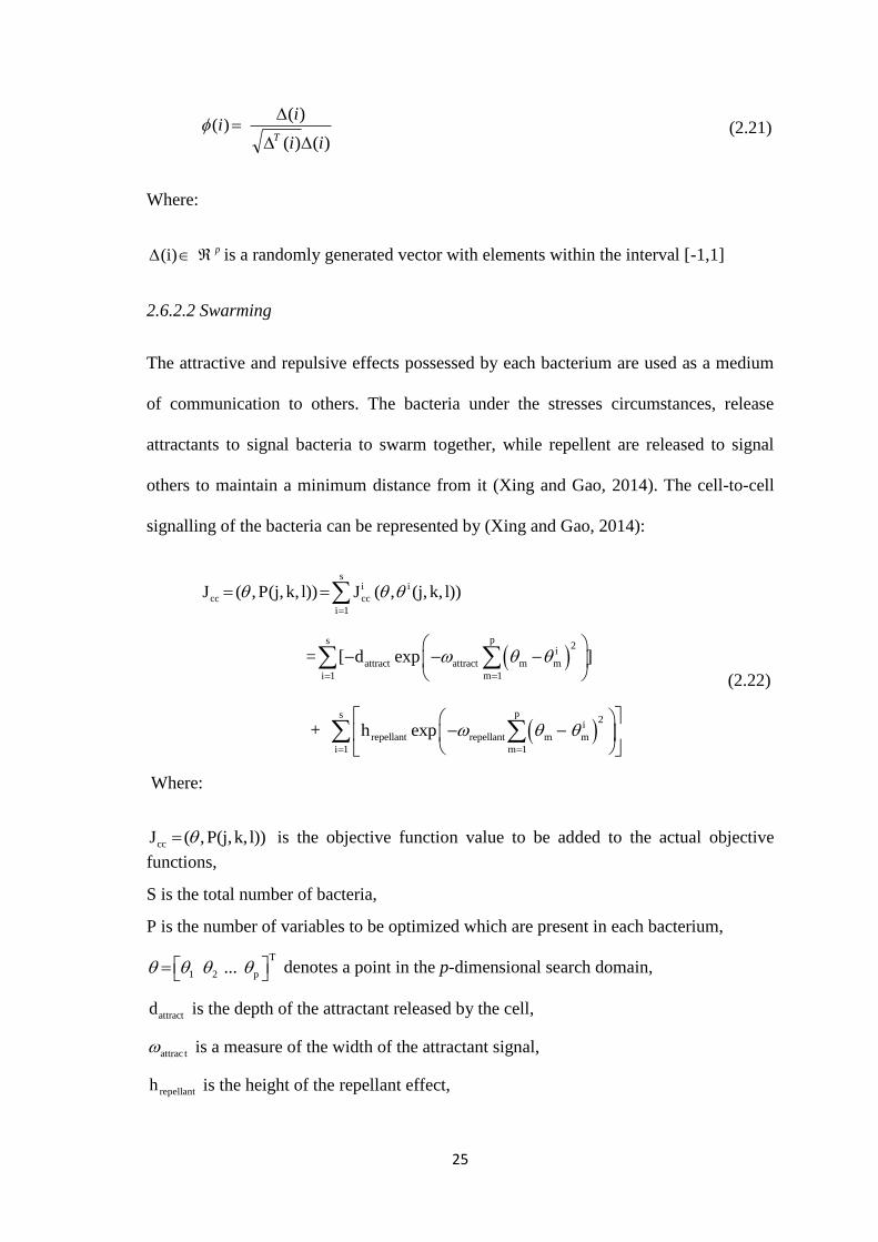
Where:
(i) p is a randomly generated vector with elements within the interval [-1,1]
2.6.2.2 Swarming
The attractive and repulsive effects possessed by each bacterium are used as a medium
of communication to others. The bacteria under the stresses circumstances, release
attractants to signal bacteria to swarm together, while repellent are released to signal
others to maintain a minimum distance from it (Xing and Gao, 2014). The cell-to-cell
signalling of the bacteria can be represented by (Xing and Gao, 2014):
si i
cc cc
i 1
J ( , P(j, k, l)) J ( , (j, k, l))
= ps
2i
attract attract m m
i 1 m 1
[ d exp ]
(2.22)
+ ps
2i
repellant repellant m m
i 1 m 1
h exp
Where:
ccJ ( ,P(j,k, l)) is the objective function value to be added to the actual objective
functions,
S is the total number of bacteria,
P is the number of variables to be optimized which are present in each bacterium,
T
1 2 p... denotes a point in the p-dimensional search domain,
attractd is the depth of the attractant released by the cell,
attrac t is a measure of the width of the attractant signal,
repellanth is the height of the repellant effect,
26
repellant is a measure of the width of the repellant.
The fitness of each position is determined by (Boussaid et al., 2013):
ccJ(i, j, k, l) J(i, j, k, l) J ( ,P(j,k, l)) (2.23)
2.6.2.3 Reproduction
The idea behind reproduction in E. Coli bacteria is that nature tends to eliminate
animals with poor foraging strategies and retain those with better ones (Kiani et al.,
2013). After cN chemotaxis steps, the reproduction step should be performed by
sorting the health of all bacteria based on fitness described by fitness function (Kiani et
al., 2013):
1
(i, j, k, l) (2.24)cN
i
health
j
J J
The rS bacteria (the population of the bacteria divided into two equal halves) with least
health due to insufficient nutrient eventually die leaving the healthiest to split into two
identical bacteria and placed at the same location (Xing and Gao, 2014).
2.6.2.4 Elimination and Dispersion
The process of elimination and dispersion is executed after reN reproduction steps in
order to avoid being involved in local optima. Each bacterium is subjected to
elimination and dispersal within the environment according to probability ( edP ). elN is
the number of elimination and dispersal steps. If a bacterium is eliminated then it is
dispersed to a new (random) location of the nutrient environment in order to maintain
the original bacteria population (Boussaid et al., 2013).
27
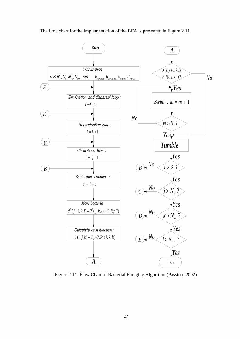
The flow chart for the implementation of the BFA is presented in Figure 2.11.
Start
E
D
C
B
E
D
C
B
No
No
No
No
No
No
EndA
Yes
Yes
Yes
Yes
Yes
( , , ) ( , , ( , , ))ccJ i j k J P j k l
Calculate cost function :
:
( 1, , ) ( , , ) ( ) ( )i i
Move bacteria
j k l j k l C i i
1
:
ii
counterBacterium
1
:
jj
loopChemotaxis
1k k
Reproduction loop :
1l l
Elimination and disparsal loop :
, , ,s c re repellant attractant attract attracth h ded
Initialization
p,S,N ,N ,N ,N , c(i),
Tumble
Yes
A
1, mmSwim
?),,,(
)1,,1,(
lkjiJ
kjiJ
?sNm
?Si
?cNj
?reNk
?edNl
Yes
Figure 2.11: Flow Chart of Bacterial Foraging Algorithm (Passino, 2002)
28
2.7 Review of Similar Works
In order to have adequate knowledge of what is obtainable presently in the area of this
research, it is very important to carry out a review of some related works done by
different authors. Below are some of the works reviewed:
Millano (2011) presented a hybrid control model of on-load tap changers. The proposed
model was based on the well-known discrete and continuous control models. The model
was designed to preserves the discrete behaviour of the tap ratio while allowing small-
signal stability and Eigen value analysis. The proposed model was tested on the
standard IEEE 14-Bus system and a real world 1488-bus model of a sub-transmission
and distribution system. However, the computational complexity of the model as
compared with the continuous method is a serious setback which involves complex
mathematical analysis.
Sagastabeitia et al., (2011) presented a remote control system for transformers with on-
load tap changer. The tool was designed and implemented in Remote Telecontrol Units
(RTU) located in transformation centres with on load tap changing capability. Its final
application is to provide an integral solution of the Telecontrol on load tap changer from
a remote operation control position (ROCP), located in the electric company’s operation
office. The main advantages of this method are: it doesn’t need a great investment to
accomplish because the automatism was implemented in existent hardware and also
only small modifications have to be made. Secondly, it reduces the number of outages
that the users could suffer unnecessarily and it also improves the quality of the electric
supply. The shortcomings of this work are; the remote system design can only control a
maximum of 8 transformers and the distance between the remote operation control
position and the devices is short (1km) and which in practice is not feasible.
29
Abdollah et al., (2013) presented the use of Artificial Bee Colony Algorithm in tuning
of ULTC for voltage regulation. Simulation results showed that the proposed method is
better than the conventional methods. However, it was observed that, increasing tap step
leads to system instability. Therefore, increasing of transformer tap step should be
carried out with careful attention and could be achieved by the application of a more
robust technique. It was also observed that the algorithm although has good exploration
capability, but exploitation capacity to find the food sources is very bad, which in turn
resulted to serious setback.
Hartung et al., (2014) presented the comparative study of tap changer control
algorithms for distribution networks with high penetration of renewables. The research
shows that on a clear day it is usually not possible to reduce the number of tap changes
and it is evident that small time delays produce best results. For cloudy days there is a
trade-off between minimum number of tap changes and compliance with the
permissible voltage band. Regulation requirements and the resistance to wear and tear
of the OLTC devices influence the optimal setting of the time delay. It was shown that
the magnitude of the voltage fluctuations can be significantly reduced by using definite
two type timers instead of simple definite timers. However, the work only provides
comparison of results obtained in different scenario but fails to address a specific
problem of concern.
Nikunj et al., (2014) presented the implementation of a fast On-Load Tap Changer
regulator. The control strategy is microcontroller based, ensuring flexibility in
programming the control algorithms. The experimental results demonstrate that the fast
OLTC is able to correct several disturbances of the ac mains besides the long duration
in variation and is much lower than the corresponding traditional regulations. However,
30
the research illustrates how micro-controller can be configured but failed to address the
decision making algorithms for the controller which select the best tap.
Shirvani et al., (2014) presented the application of on-load tap changer for voltage
control. The research aimed at showing the effects of on-load tap changers for voltage
control as well as showing OLTC on power system performance. A typical test system
installed with OLTC is investigated following change in input voltage. Simulation
results showed the effectiveness of OLTC in regaining the system voltage after drip.
However, delay in fast response of the voltage back to normalcy is a shortcoming.
Therefore, a smart method of tuning the OLTC is required to limit the time of operation
of the OLTC.
Rolga et al., (2015) presented the different methods of on load tap changer selection
such as Remote control system, Solid state on load tap changer using microcontroller
and supervisory control and data acquisition (SCADA). Finally, the research showed
that SCADA has more advantages than the remote control system and solid state on
load tap changer using microcontroller. The SCADA can control a number of
substations by a single SCADA centre. It can store a very large amount of data and the
data can be displayed in anyway the user wants. Data can be viewed from anywhere not
just on site. The shortcomings of this method are it uses communication network which
is usually associated with noise, interference and network failure. So, an in built and
highly intelligent system is required.
Rolga et al., (2015) presented tap changing in parallel operated transformers using
SCADA where transformers are connected in parallel to meet the increasing loads
demand in power system. The parallel operation of tap changing transformers is done
by using the remote tap changer control cubicle (RTCC), which control the tap
31
changing of parallel connected transformers from the control room near the yard. The
main advantages of SCADA compared to RTCC are to minimize fault response time,
reduce planned down times, reduce operations overhead, reduce manpower requirement
and maximize equipment lifetime. But there are many drawbacks since SCADA system
uses communication networks, such as noise, interference and network failure. As such,
meta-heuristic algorithms are more efficient and robust than the SCADA as they don’t
need an external communication network.
Vigneshwaran and Yuvaraja, (2015) presented voltage regulation by solid state tap
changer mechanism for distribution transformer. The research deals with the
replacement of conventional electro-mechanical way of on load tap changers with the
solid state tap changers for voltage regulation. The research shows that with fully
electronic control of tap changing the problems associated with the mechanical on load
tap changing which include excessive conduction losses, slow operation and arcing in
the diverter switch have been properly rectified. The sequential switching of the
thyristor using Pulse Width Modulation (PWM) to regulate the voltage based on the
voltage feedback taken from the output side was adopted. However, its major
disadvantage is that when two thyristors are turn ON over short period during the tap
changing process, the circuit of the diverter switch gets burnt; which in turn reduces the
reliability of the system.
Gohil and Verma, (2016) presented the review on influence of the transformer tap
changer on voltage stability. The review provides different methods of achieving
voltage stability such as small and large disturbance stability. Steady state voltage
stability is concerned with the limits on the existence of steady state operating points on
the network. FACTS devices can be utilized to increase the transmission capability, the

32
stability margin and dynamic behaviour or serve to improve power quality. The research
proposed the use of on-load tap changer for voltage control in power system network.
The algorithm was developed for voltage level control with on-load tap changer
operation. However, the research fails to consider any of the standard test bed as a
framework for comparison.
Babu and Varghese, (2016) presented voltage compensation of OLTC transformer using
Proportional Integrator (PI) controller. PSCAD platform was used for the simulation.
The result shows that the proposed approach is capable of raising the voltage to some
limits. However, the results obtained failed to reach the load voltage requirement.
Therefore, a more robust technique is needed to compensate the voltage to the load
voltage level.

33
CHAPTER THREE
MATERIALS AND METHODS
3.1 Introduction
In this chapter, an elaborate procedure for the actualization of the work is discussed.
The materials employed and the parameters setting used for the BFA algorithm, the
minimum and maximum voltage limits as well as the OLTC limits are presented. Also,
a comprehensive methodology adopted for this work is given.
3.2 Materials
The materials employed for the actualization of this research are as follows:
3.2.1 Computer Specifications
All simulation analyses were carried out using SAMSUNG DESKTOP QEQ2NTB
computer with the following specifications:
i. Intel(R) Pentium (R) CPU B8950;
ii. 2.10GHz 64-based processor;
iii. 4.00GB installed memory (RAM) and;
iv. 64-bit windows 10 Operating System (OS).
3.2.2 MATLAB 2016a Software
Simulations were performed under virtual platform using MATLAB 2016a, PSAT
Toolbox for analysis. The details of the codes for both ABC and BFA are provided in
appendix B1.

34
3.2.3 Network Parameters
The standard IEEE 14-bus and a dedicated Nigerian 32-bus power system network with
the following network parameters: slack bus, active and reactive powers, bus voltages
and bus voltage angles have been adopted for this research.
3.3 Methodology
The objectives as outlined are achieved in line with the following procedures:
3.3.1 Acquisition of Relevant Networks Data
Data of the standard IEEE 14-bus test network and the Nigerian 32-bus power system
network used are:
i. Line data (resistance and reactance of each line in ohms)
ii. Bus data (active and reactive power demand in kW and kVAr respectively)
iii. Network base voltage
iv. Sending and receiving end buses
3.3.2 Base-case Power Flow Analysis
The pseudo-code used in developing the algorithm for running the base-case power
flow analysis of the transmission networks are presented below; and the complete flow
chart is shown in Figure 3.1.
i. Load the network line and bus data
ii. Assume a flat start voltage profile of 1.0 p.u at all buses
iii. Calculate the voltage and phase angle at each bus of the network
iv. Compute the line losses ( ik ikP and Q ) using equations (2.8) and (2.9)
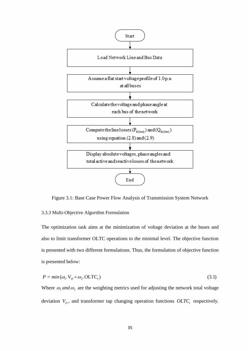
35
Figure 3.1: Base Case Power Flow Analysis of Transmission System Network
3.3.3 Multi-Objective Algorithm Formulation
The optimization task aims at the minimization of voltage deviation at the buses and
also to limit transformer OLTC operations to the minimal level. The objective function
is presented with two different formulations. Thus, the formulation of objective function
is presented below:
P = min 1 2( .V .OLTC ) (3.1)D t
Where 1 2and are the weighting metrics used for adjusting the network total voltage
deviation DV , and transformer tap changing operation functions tOLTC respectively.
36
Due to the equal importance attached to both objectives in equation (3.1), a unit
weighting metric was assigned to both objective functions. Thus, 1 = 2
3.3.3.1 Constraints
The optimal tuning of OLTC transformer is considered as a constrained optimization
problem that deals with the equality and inequality constraints.
Equality Constraints
The equality constraints represent equations expressed as:
.min .max (3.2)Tr Tr Trtap tap tap
min max (3.3)bus bus busQ Q Q
In equality Constraints
The system operating constraints constitute the in-equality constraints on the dependent
variables such as the voltage magnitude of the buses, current through the cables, line
and transformer flow limits. They have the form described in the following equations:
min max (3.4)V V V
lim (3.5)i i
lim (3.6)s s
The network voltage constraint limits has been set as 0.85p.u and 1.15p.u for
min maxV and V respectively.
37
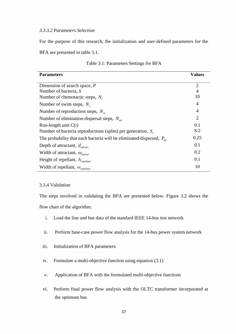
3.3.3.2 Parameters Selection
For the purpose of this research, the initialization and user-defined parameters for the
BFA are presented in table 3.1.
Table 3.1: Parameters Settings for BFA
Parameters Values
Dimension of search space, P 2
Number of bacteria, S 4
Number of chemotactic steps, cN 10
Number of swim steps, sN 4
Number of reproduction steps, reN 4
Number of elimination-dispersal steps, edN 2
Run-length unit C(i) 0.1
Number of bacteria reproductions (splits) per generation, rS S/2
The probability that each bacteria will be eliminated/dispersed, edP 0.25
Depth of attractant, attractd 0.1
Width of attractant, attract 0.2
Height of repellant, repellanth 0.1
Width of repellant, repellant 10
3.3.4 Validation
The steps involved in validating the BFA are presented below. Figure 3.2 shows the
flow chart of the algorithm.
i. Load the line and bus data of the standard IEEE 14-bus test network
ii. Perform base-case power flow analysis for the 14-bus power system network
iii. Initialization of BFA parameters
iv. Formulate a multi-objective function using equation (3.1)
v. Application of BFA with the formulated multi-objective functions
vi. Perform final power flow analysis with the OLTC transformer incorporated at
the optimum bus
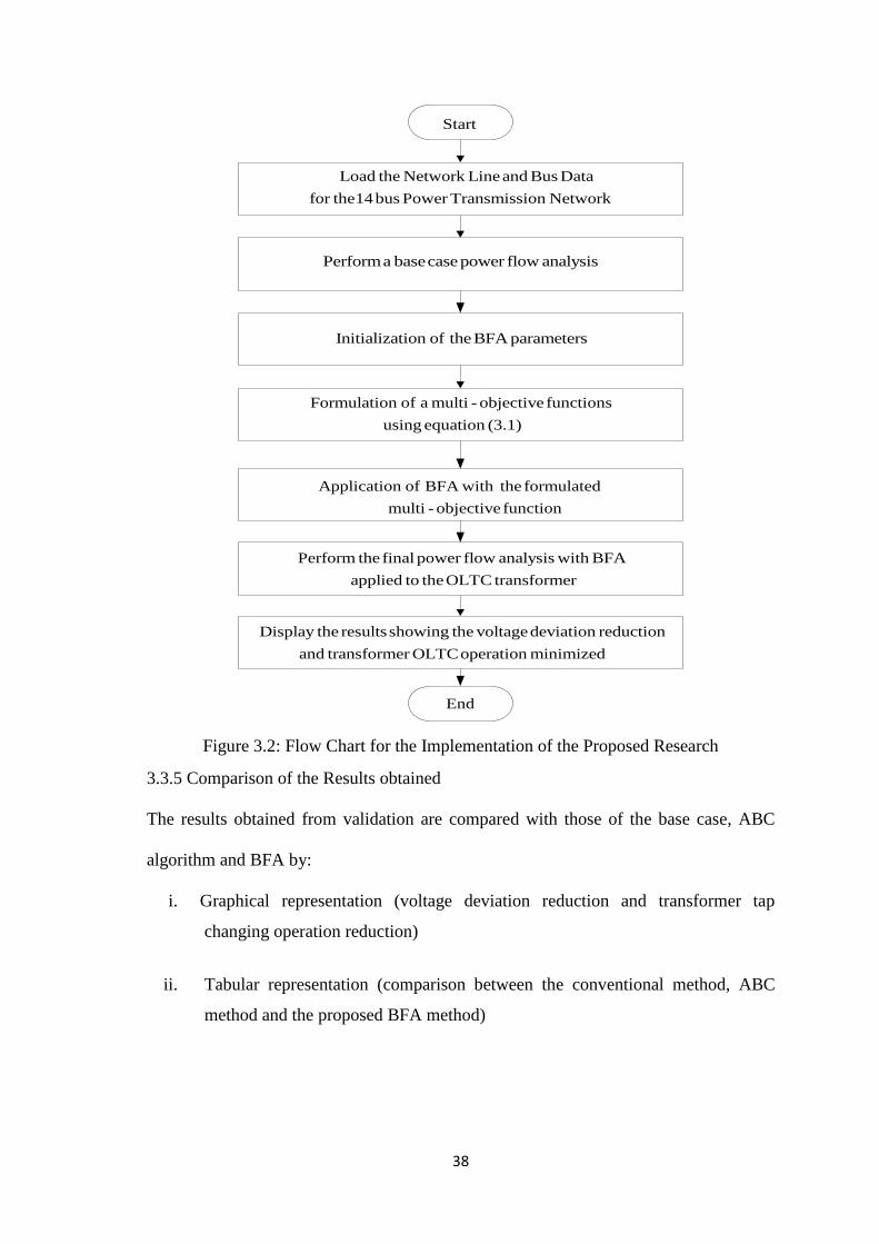
38
Start
End
Load the Network Lineand Bus Data
for the14bus Power Transmission Network
Performa basecasepower flow analysis
Initialization of theBFA parameters
Formulation of a multi - objective functions
using equation (3.1)
Application of BFA with the formulated
multi - objective function
Perform thefinal power flow analysis with BFA
applied to theOLTC transformer
Display the resultsshowing the voltagedeviation reduction
and transformer OLTCoperation minimized
Figure 3.2: Flow Chart for the Implementation of the Proposed Research
3.3.5 Comparison of the Results obtained
The results obtained from validation are compared with those of the base case, ABC
algorithm and BFA by:
i. Graphical representation (voltage deviation reduction and transformer tap
changing operation reduction)
ii. Tabular representation (comparison between the conventional method, ABC
method and the proposed BFA method)

39
3.3.6 Implementation of the results on the Nigerian 32-bus Power System Network
The results will finally be implemented on the Nigerian power system network in order
to test the performance and effectiveness of the proposed approach using graphical and
tabular form representation.
40
CHAPTER FOUR
RESULTS AND DISCUSSIONS
4.1 Introduction
In this chapter, results and discussion of the theoretical concepts from the previous two
chapters are presented. The effectiveness of the BFA is validated on the standard IEEE
14-bus power system network and comparison was made between the ABC and BFA. A
real 32-bus Nigerian power system network was considered for implementation of the
proposed technique. In both networks, two different cases were considered for analysis.
Case I: Network without BFA (Base-case) and
Case II: Network with BFA
4.2 The Standard IEEE 14-Bus Power System Network
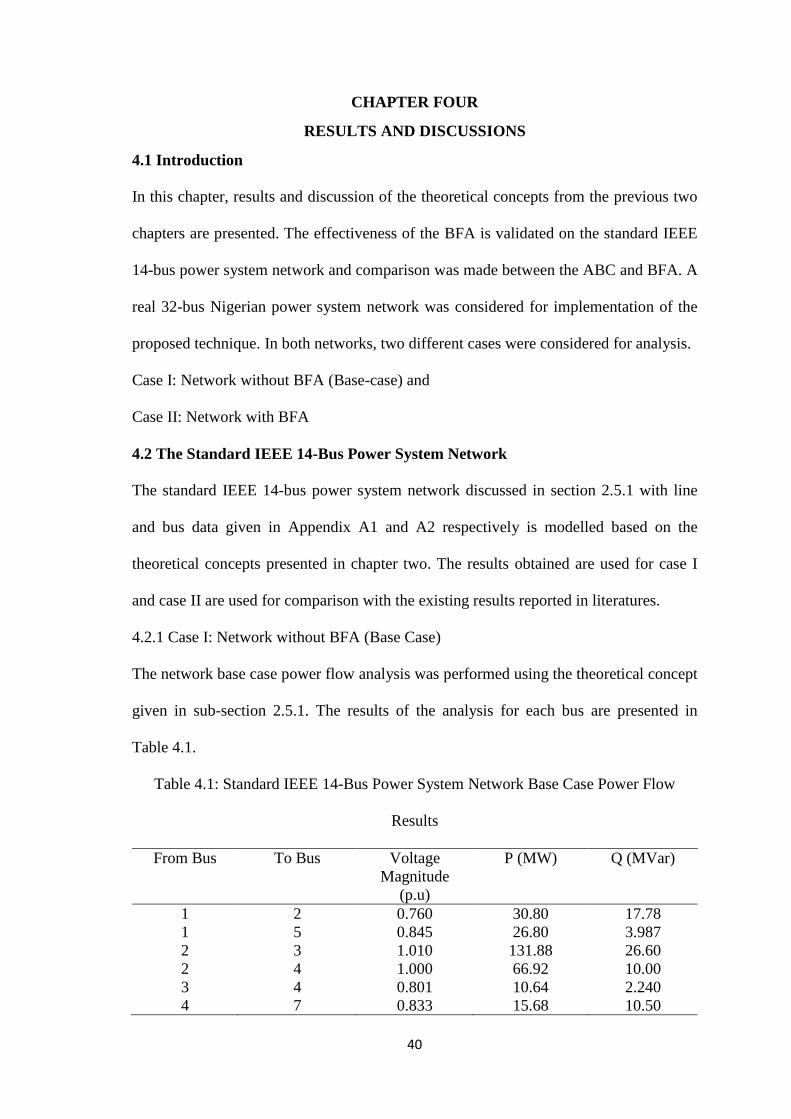
The standard IEEE 14-bus power system network discussed in section 2.5.1 with line
and bus data given in Appendix A1 and A2 respectively is modelled based on the
theoretical concepts presented in chapter two. The results obtained are used for case I
and case II are used for comparison with the existing results reported in literatures.
4.2.1 Case I: Network without BFA (Base Case)
The network base case power flow analysis was performed using the theoretical concept
given in sub-section 2.5.1. The results of the analysis for each bus are presented in
Table 4.1.
Table 4.1: Standard IEEE 14-Bus Power System Network Base Case Power Flow
Results
From Bus To Bus Voltage
Magnitude
(p.u)
P (MW) Q (MVar)
1 2 0.760 30.80 17.78
1 5 0.845 26.80 3.987
2 3 1.010 131.88 26.60
2 4 1.000 66.92 10.00
3 4 0.801 10.64 2.240
4 7 0.833 15.68 10.50
41
From Bus To Bus Voltage
Magnitude
(p.u)
P(MW) Q(MVar)
7 8 1.000 6.876 6.345
7 9 1.090 3.987 5.345
5 6 1.160 41.30 23.24
6 12 1.000 12.60 8.12
6 13 1.000 4.900 2.52
12 13 1.000 8.540 2.24
13 14 1.171 18.90 8.12
9 10 1.103 20.86 7.000
4.2.2 Case II: Network with BFA
After the network base case power flow analysis results were obtained, the BFA in sub-
section 2.6.2 was then applied to the standard 14 bus network. The results obtained after
final power flow analysis with the application of BFA showed a reduction of voltage
deviation from the defined limits. A clear picture of the effect of BFA on the
minimization of voltage deviation is given in Table 4.2.
Table 4.2: Standard IEEE 14-Bus Power System Network Power Flow Results using
BFA
From Bus To Bus Voltage
Magnitude
(p.u)
P (MW) Q (MVar)
1 2 1.129 30.30 16.72
1 5 1.010 25.80 2.987
2 3 1.011 132.88 24.50
2 4 0.999 65.92 9.501
3 4 1.010 10.04 2.240
4 9 0.965 14.68 10.50
7 8 0.990 7.876 6.345
7 9 1.000 2.987 5.345
5 6 1.120 40.30 23.24
6 11 1.173 11.70 7.120
11 10 1.020 4.954 2.521
12 13 1.102 9.540 1.241
13 14 1.000 17.90 7.020
9 14 0.852 21.86 7.112
42
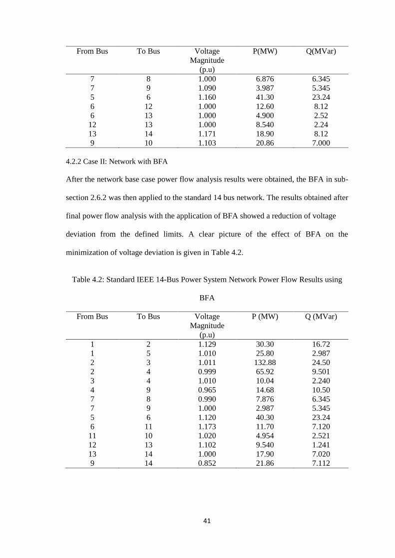
4.2.3 Network Bus Voltage Deviation Reduction using Base case and ABC Algorithm
The application of ABC algorithm to the standard IEEE 14 Bus network has reduced the
bus voltage deviation of the entire network as shown in Table 4.1. The bus voltage
magnitudes shown in Figure 4.1 are plotted against their corresponding time. A clear
reduction in bus voltage deviation was recorded from the graph using the Base case and
ABC algorithm shown in Figure 4.1.
The bus voltage deviation of the network was reduced using the base case and the ABC
algorithm by 1.0125% and 1.0112% respectively. It was also seen from the graph that
the computational time was reduced from 6.67sec to 4.37sec respectively.
Figure 4.1: Bus Voltage Deviation Reduction using the Base case and ABC algorithm
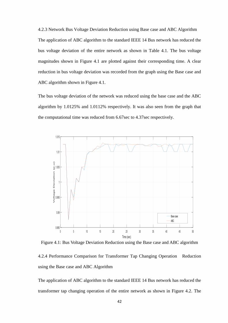
4.2.4 Performance Comparison for Transformer Tap Changing Operation Reduction
using the Base case and ABC Algorithm
The application of ABC algorithm to the standard IEEE 14 Bus network has reduced the
transformer tap changing operation of the entire network as shown in Figure 4.2. The
43
transformer tap ratios shown in Figure 4.2 are plotted against their corresponding time.
A clear reduction in transformer tap changing operation was recorded from the graph
using the Base case and ABC algorithm shown in Figure 4.1.
The entire transformer tap changing operation of the network was reduced using the
base case and the ABC algorithm by 0.6 %. It was also seen from the graph that the
settling time was reduced from 50sec to 20sec respectively as in figure 4.2.
Figure 4.2: Transformer Tap changing operation Reduction using the Base case and
ABC
The performance results for both cases of the network using the Base case and ABC are
summarized in Table 4.3.
44
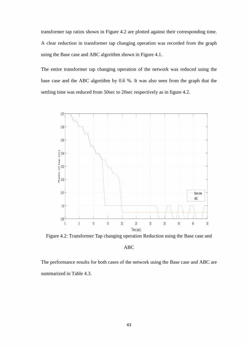
Table 4.3: Summary of Simulation Results for the 14-bus Standard IEEE Power System
Network using the base case and ABC algorithm
Parameter
Description Base case ABC
Total Bus Voltage
Deviation
Reduction
1.0125 1.0112
Percentage
Reduction in Bus
Voltage Deviation
(%)
- 0.25
Total Tap
Changing
Operations
Reduction
0.9102 0.8975
Percentage
Reduction in Tap
changing
operations (%)
- 0.6
Reduction in
Computational
Time (sec)
6.67 4.32
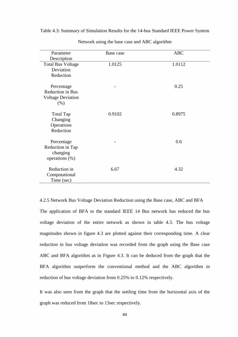
4.2.5 Network Bus Voltage Deviation Reduction using the Base case, ABC and BFA
The application of BFA to the standard IEEE 14 Bus network has reduced the bus
voltage deviation of the entire network as shown in table 4.3. The bus voltage
magnitudes shown in figure 4.3 are plotted against their corresponding time. A clear
reduction in bus voltage deviation was recorded from the graph using the Base case
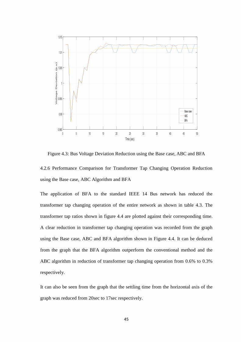
ABC and BFA algorithm as in Figure 4.3. It can be deduced from the graph that the
BFA algorithm outperform the conventional method and the ABC algorithm in
reduction of bus voltage deviation from 0.25% to 0.12% respectively.
It was also seen from the graph that the settling time from the horizontal axis of the
graph was reduced from 18sec to 13sec respectively.
45
Figure 4.3: Bus Voltage Deviation Reduction using the Base case, ABC and BFA
4.2.6 Performance Comparison for Transformer Tap Changing Operation Reduction
using the Base case, ABC Algorithm and BFA
The application of BFA to the standard IEEE 14 Bus network has reduced the
transformer tap changing operation of the entire network as shown in table 4.3. The
transformer tap ratios shown in figure 4.4 are plotted against their corresponding time.
A clear reduction in transformer tap changing operation was recorded from the graph
using the Base case, ABC and BFA algorithm shown in Figure 4.4. It can be deduced
from the graph that the BFA algorithm outperform the conventional method and the
ABC algorithm in reduction of transformer tap changing operation from 0.6% to 0.3%
respectively.
It can also be seen from the graph that the settling time from the horizontal axis of the
graph was reduced from 20sec to 17sec respectively.
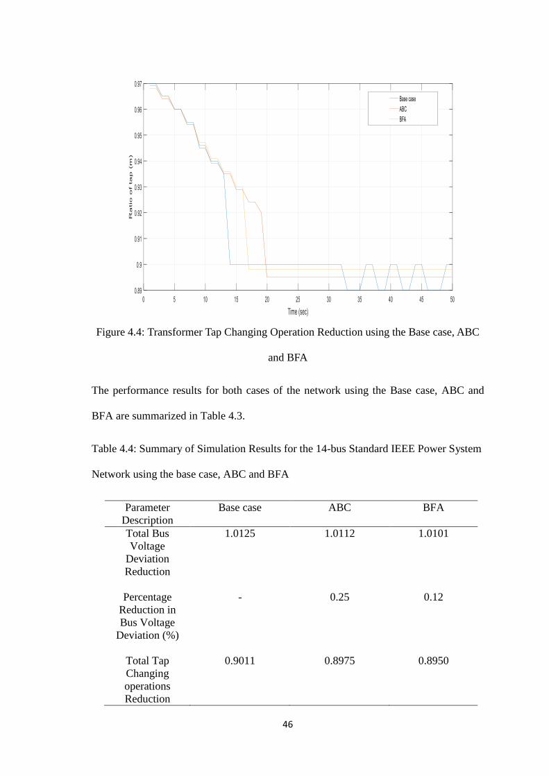
46
Figure 4.4: Transformer Tap Changing Operation Reduction using the Base case, ABC
and BFA
The performance results for both cases of the network using the Base case, ABC and
BFA are summarized in Table 4.3.
Table 4.4: Summary of Simulation Results for the 14-bus Standard IEEE Power System
Network using the base case, ABC and BFA
Parameter
Description Base case ABC BFA
Total Bus
Voltage
Deviation
Reduction
1.0125 1.0112 1.0101
Percentage
Reduction in
Bus Voltage
Deviation (%)
- 0.25 0.12
Total Tap
Changing
operations
Reduction
0.9011 0.8975 0.8950
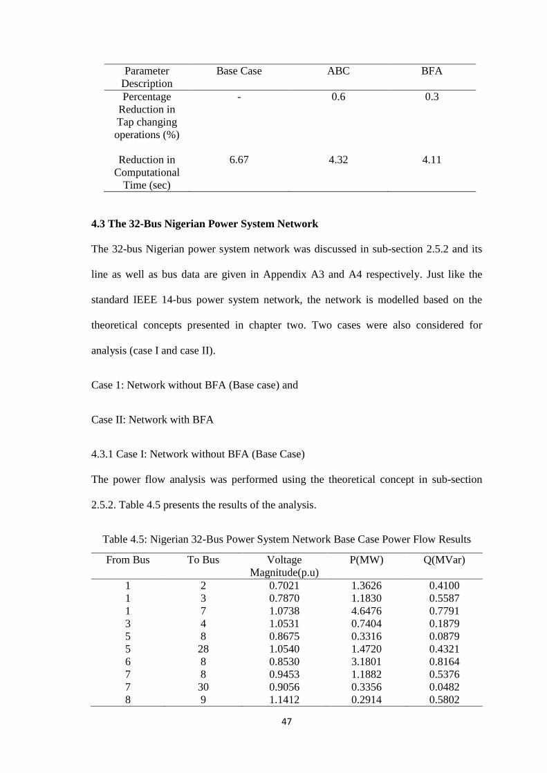
47
Parameter
Description
Base Case ABC BFA
Percentage
Reduction in
Tap changing
operations (%)
- 0.6 0.3
Reduction in
Computational
Time (sec)
6.67 4.32 4.11
4.3 The 32-Bus Nigerian Power System Network
The 32-bus Nigerian power system network was discussed in sub-section 2.5.2 and its
line as well as bus data are given in Appendix A3 and A4 respectively. Just like the
standard IEEE 14-bus power system network, the network is modelled based on the
theoretical concepts presented in chapter two. Two cases were also considered for
analysis (case I and case II).
Case 1: Network without BFA (Base case) and
Case II: Network with BFA
4.3.1 Case I: Network without BFA (Base Case)
The power flow analysis was performed using the theoretical concept in sub-section
2.5.2. Table 4.5 presents the results of the analysis.
Table 4.5: Nigerian 32-Bus Power System Network Base Case Power Flow Results
From Bus To Bus Voltage
Magnitude(p.u)
P(MW) Q(MVar)
1 2 0.7021 1.3626 0.4100
1 3 0.7870 1.1830 0.5587
1 7 1.0738 4.6476 0.7791
3 4 1.0531 0.7404 0.1879
5 8 0.8675 0.3316 0.0879
5 28 1.0540 1.4720 0.4321
6 8 0.8530 3.1801 0.8164
7 8 0.9453 1.1882 0.5376
7 30 0.9056 0.3356 0.0482
8 9 1.1412 0.2914 0.5802
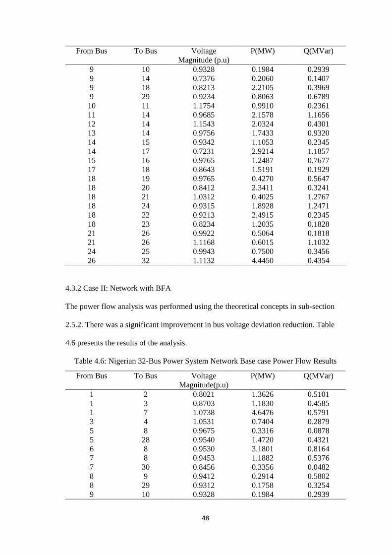
48
From Bus To Bus Voltage
Magnitude (p.u)
P(MW) Q(MVar)
9 10 0.9328 0.1984 0.2939
9 14 0.7376 0.2060 0.1407
9 18 0.8213 2.2105 0.3969
9 29 0.9234 0.8063 0.6789
10 11 1.1754 0.9910 0.2361
11 14 0.9685 2.1578 1.1656
12 14 1.1543 2.0324 0.4301
13 14 0.9756 1.7433 0.9320
14 15 0.9342 1.1053 0.2345
14 17 0.7231 2.9214 1.1857
15 16 0.9765 1.2487 0.7677
17 18 0.8643 1.5191 0.1929
18 19 0.9765 0.4270 0.5647
18 20 0.8412 2.3411 0.3241
18 21 1.0312 0.4025 1.2767
18 24 0.9315 1.8928 1.2471
18 22 0.9213 2.4915 0.2345
18 23 0.8234 1.2035 0.1828
21 26 0.9922 0.5064 0.1818
21 26 1.1168 0.6015 1.1032
24 25 0.9943 0.7500 0.3456
26 32 1.1132 4.4450 0.4354
4.3.2 Case II: Network with BFA
The power flow analysis was performed using the theoretical concepts in sub-section
2.5.2. There was a significant improvement in bus voltage deviation reduction. Table
4.6 presents the results of the analysis.
Table 4.6: Nigerian 32-Bus Power System Network Base case Power Flow Results
From Bus To Bus Voltage
Magnitude(p.u)
P(MW) Q(MVar)
1 2 0.8021 1.3626 0.5101
1 3 0.8703 1.1830 0.4585
1 7 1.0738 4.6476 0.5791
3 4 1.0531 0.7404 0.2879
5 8 0.9675 0.3316 0.0878
5 28 0.9540 1.4720 0.4321
6 8 0.9530 3.1801 0.8164
7 8 0.9453 1.1882 0.5376
7 30 0.8456 0.3356 0.0482
8 9 0.9412 0.2914 0.5802
8 29 0.9312 0.1758 0.3254
9 10 0.9328 0.1984 0.2939
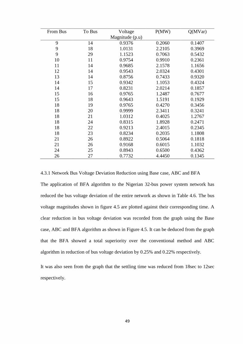
49
From Bus To Bus Voltage
Magnitude (p.u)
P(MW) Q(MVar)
9 14 0.9376 0.2060 0.1407
9 18 1.0131 2.2105 0.3969
9 29 1.1523 0.7063 0.5432
10 11 0.9754 0.9910 0.2361
11 14 0.9685 2.1578 1.1656
12 14 0.9543 2.0324 0.4301
13 14 0.8756 0.7433 0.9320
14 15 0.9342 1.1053 0.4324
14 17 0.8231 2.0214 0.1857
15 16 0.9765 1.2487 0.7677
15 18 0.9643 1.5191 0.1929
18 19 0.9765 0.4270 0.3456
18 20 0.9999 2.3411 0.3241
18 21 1.0312 0.4025 1.2767
18 24 0.8315 1.8928 0.2471
18 22 0.9213 2.4015 0.2345
18 23 0.8234 0.2035 1.1808
21 26 0.8922 0.5064 0.1818
21 26 0.9168 0.6015 1.1032
24 25 0.8943 0.6500 0.4362
26 27 0.7732 4.4450 0.1345
4.3.1 Network Bus Voltage Deviation Reduction using Base case, ABC and BFA
The application of BFA algorithm to the Nigerian 32-bus power system network has
reduced the bus voltage deviation of the entire network as shown in Table 4.6. The bus
voltage magnitudes shown in figure 4.5 are plotted against their corresponding time. A
clear reduction in bus voltage deviation was recorded from the graph using the Base
case, ABC and BFA algorithm as shown in Figure 4.5. It can be deduced from the graph
that the BFA showed a total superiority over the conventional method and ABC
algorithm in reduction of bus voltage deviation by 0.25% and 0.22% respectively.
It was also seen from the graph that the settling time was reduced from 18sec to 12sec
respectively.
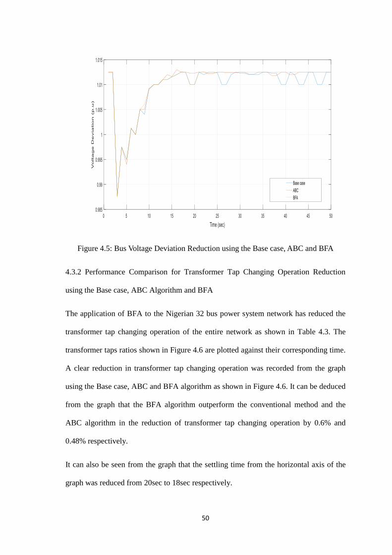
50
Figure 4.5: Bus Voltage Deviation Reduction using the Base case, ABC and BFA
4.3.2 Performance Comparison for Transformer Tap Changing Operation Reduction
using the Base case, ABC Algorithm and BFA
The application of BFA to the Nigerian 32 bus power system network has reduced the
transformer tap changing operation of the entire network as shown in Table 4.3. The
transformer taps ratios shown in Figure 4.6 are plotted against their corresponding time.
A clear reduction in transformer tap changing operation was recorded from the graph
using the Base case, ABC and BFA algorithm as shown in Figure 4.6. It can be deduced
from the graph that the BFA algorithm outperform the conventional method and the
ABC algorithm in the reduction of transformer tap changing operation by 0.6% and
0.48% respectively.
It can also be seen from the graph that the settling time from the horizontal axis of the
graph was reduced from 20sec to 18sec respectively.
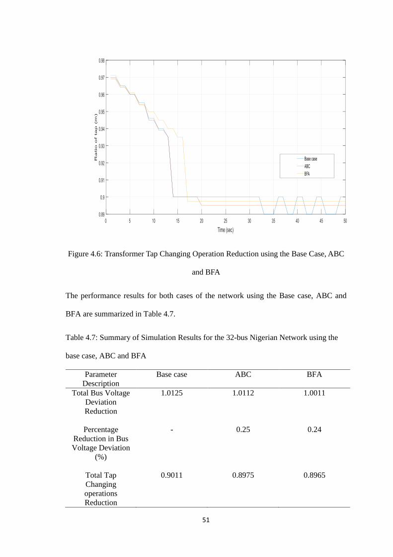
51
Figure 4.6: Transformer Tap Changing Operation Reduction using the Base Case, ABC
and BFA
The performance results for both cases of the network using the Base case, ABC and
BFA are summarized in Table 4.7.
Table 4.7: Summary of Simulation Results for the 32-bus Nigerian Network using the
base case, ABC and BFA
Parameter
Description Base case ABC BFA
Total Bus Voltage
Deviation
Reduction
1.0125 1.0112 1.0011
Percentage
Reduction in Bus
Voltage Deviation
(%)
- 0.25 0.24
Total Tap
Changing
operations
Reduction
0.9011 0.8975 0.8965

52
Parameter
Description
Base Case ABC BFA
Percentage
Reduction in Tap
changing
operations (%)
- 0.6 0.48
Reduction in
Computational
Time (sec)
6.67 4.32 4.31
53
CHAPTER FIVE
CONCLUSION AND RECOMMENDATION
5.1 Summary
This chapter presents a detailed summary of the research findings. The research has
applied a Bacterial Foraging Algorithm based for tuning of on-load tap changing
transformer for voltage regulation in power transmission network. The research has
finally resulted in reducing the voltage at the bus to the required limits; and transformer
tap changing operation was also reduced which in turn increase the system stability.
5.2 Conclusion
When applied the algorithm on the 14-bus IEEE standard test network, the BFA has
demonstrated its superiority over the conventional method and ABC algorithms in terms
of reduction in bus voltage deviation by (0.25%) and (0.12%) and reduction in
transformer taps changing operation by (0.6%) and (0.3%) respectively.
On the 32-bus Nigerian power system network, the BFA has shown a total superiority
over the conventional method and ABC algorithms in all parameters with 4.31%, 0.22%
and 0.48% reduction in computational time, bus voltage deviation and transformer tap
changing operation respectively;
5.3 Significant Contributions
Numerous researches on tuning of on-load tap changer in transmission system networks
have been carried out and reported in literatures. Also, a significant number of
researches have employed different approaches in actualizing their results. The
substantial contributions of this research work are enumerated as follows:
i. The use of BFA in tuning of OLTC transformer for voltage regulation in power
transmission networks.

54
ii. Implementation of the proposed approach on the Nigerian 32-Bus power system
networks which led to reduction in bus voltage deviation and transformer taps
changing operation from 0.25% to 0.22% and 0.6% to 0.48% respectively.
5.4 Recommendations for Further works
The following possible areas of further work are recommended for consideration for
future research:
i. The research can be extended to other members of swarm intelligence meta-
heuristic algorithms such as AFSA, CSO etc.
ii. The use of BFA in tuning of OLTC transformer for voltage regulation in radial
distribution network can also be considered.
55
REFERENCES
Abdollah, F. H. (2013). Tuning under load tap changer (ULTC) controller by using
Artificial Bee Colony Algorithm for voltage regulation. International society of
academic and industrial research.
Acha V.G., Agelidis, O. (2010). Power Electronic Control in Electrical Systems.
Newnes power Engineering series.
Aimilia Theologi, M. (2016). Metaheuristics-Based optimal management of reactive
sources in offshore wind farms.
Babu Bateena, J. V. (2016). Voltage compensation of OLTC Transformer using PI
Controller. International Journal of Advanced research in Electrical,
Electronics and Instrumentation Engineering.
Boussaid I, L. J. (2013). A Survey on optimization metaheuristics. Information
Sciences.
Cai, L. (2010). Robust Co-ordinated Control of FACTS Devices in large power
systems. Ph.D Thesis, University of Duisburg Germany.
Karaboga, D. B. B. (2007). A Powerful and efficient algorithm for numerical function
optimization: artificial bee colony (ABC) Algorithm. Journal of global
optimization, 459-71.
Dai, F. (2012). Voltage Control of Distributed Network with distributed Generation.
International conference on Development in power systems protection.
Bermingham.
Martinez, I. Fernendez, (2013). Thyristor based Solid state tap changer for distribution
transformers. 2013 IEEE 11th international Workshop of Electronics, control,
measurements, signals and their applications on mechatronics. Toulouse.
Eseosa, O. a. (2015). Efficiciency improvement of Nigerian 330kV network using
flexible alternating current transmission systems (FACTS) devices.
International Journal of Advances in Engineering and Technology.
Fusco and M. Russo. (2007). Adaptive Voltage Control in power systems modelling,
Design and Applications Berlin. Springers, Advances in industrial control.
Ram., G.C. Moulli.-M. (2015). Design of a power electronic - Assisted OLTC for Grid
voltage regulation,. IEEE Transactions in Power Delivery.
Hashemi Z., Mardaneh. M. (2011). Fuzzy Logic Controller to Improve the Coordination
of Cascaded Tap Changers. Australian Journal of Basic and Applied Sciences.
Sagastabeitia., K.J. Zamora and Ajinako, (2011). Remote Control System for
Transformers with On-Load Tap Changer. 87-92.
56
Kiani M.,. (2013). A Bacterial foraging Optimization Approach for Tuning type-2 fuzzy
controller. Turkish Journal of Electrical Engineering and Computer sciences.
Salem., M.R. (2007). Voltage control by tap changing transformers for a radial
distribution network.
Hartung, E. M. B. (2014). Comparative Study of tap-changer control algorithms for
distribution networks with high penetration of renewables. CIRED Workshop.
Milano (2011). Hybrid Control Model of Under Load Tap Changers. IEEE Transactions
on power Delivery.
Ming, N. C. (2014). A review on application of heuristic optimization algorithms for
optimal power flow in modern power systems. Journal of modern power systems
and clean energy, 289-297.
Mohammed, Z. H. (2011). Fuzzy Logic Controller to improve the Coordination of
Cascaded Tap Changers. Australian Journal of Basic and Applied Sciences.
Shirvani, M. A. (2014). Application of on-load tap changer for voltage control.
Advances in Natural and applied sciences, 920-924.
Nadeem D. Saeed R., (2013). Fully Electronic Tap Changer Control, IEEE Conference
on Clean Energy and Technology, Langkawi.
Nikunj R. Patel, M. M. (2014). Solid-State On Load Tap Changer for Transformer
Using Micro-controller. International Journal of Engineering Development And
Research.
Passino K., (2002). Biomimicry of Bacterial Foraging for distributed optimization and
control. Control System IEEE standard.
Prada Bianco. R., Seelig. J. (2003). Modelling on load tap changer voltage control and
limits for network loading and voltage control effectiveness assessment. Power
technical conference proceedings, IEEE Bologna.
Rolga Roy, A. S. (2015). Comparison Study of Different Methods of on Load Tap
Changer. International Journal of Advanced Research in Electrical, Electronics
and Instrumentation Engineering.
Rolga Roy, S. J. (2015). Tap changing in parallel operated transformers using SCADA.
international journal of advanced research in electrical, electronics and
instrumentation engineering.
Romero, D. (2010). Voltage Regulation in Distribution systems Tap changer and Wind
Power, lund. Faculty of Engineering, Lund University,.
Saadat. (2010). Power system analysis and control. PSA Publishing.
57
Siahkolah, J. Faiz (2006). Electronic Tap Changer for Distribution systems
transformers. Berlins springer.
Gohil, M. Verma. (2016). Review on influence of the Transformer Tap changer on
voltage stability. International Journal for Technological Research in
Engineering.
Stott, B. (2009). Effective starting process for Newton Raphson load flows. Proc. IEEE.
Hashim T., A. Mardaneh, (2012). A Review on voltage control methods for active
distribution networks,. Electrical Review, 304-312.
Tinney W.F., H. C. (2012). Power flow solutions by newtons method. IEEE Trans.,.
Vigneshwaran S., and Yuvaraja T., (2015). Voltage Regulation by Solid State Tap
Change Mechanism for Distributing Transformer. International Journal of
Engineering Research and Tecnology.
Liao, J. Z. (2013). An adaptive chaotic artificial bee colony algorithm for short-term
hydrothermal generation scheduling . International Journal of Electrical Power
and Energy Systems, 34-42.
Viawan., F.A. (2008). Voltage control and voltage stability of power Distribution
systems in the pressence of Distributed Generations. Chalmers University of
Technology.
Xing B., Gao. W. (2014). Innovative Computational intelligence: A rough guide to
clever algorithm.
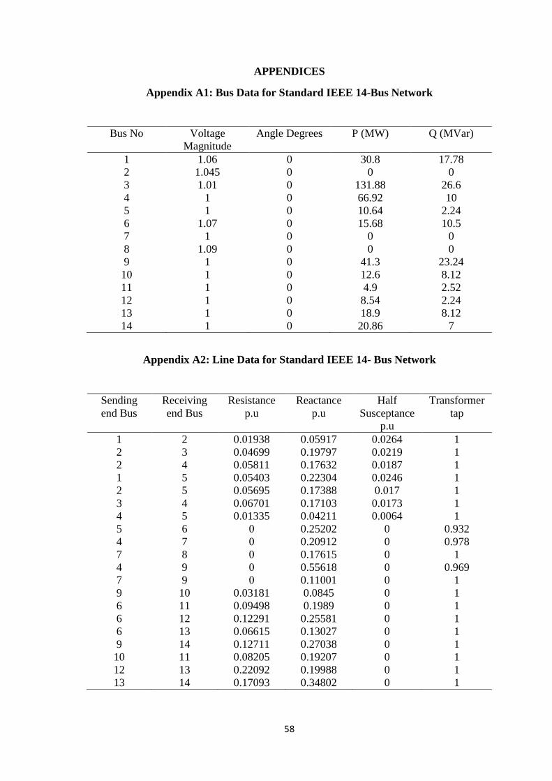
58
APPENDICES
Appendix A1: Bus Data for Standard IEEE 14-Bus Network
Bus No Voltage
Magnitude
Angle Degrees P (MW) Q (MVar)
1 1.06 0 30.8 17.78
2 1.045 0 0 0
3 1.01 0 131.88 26.6
4 1 0 66.92 10
5 1 0 10.64 2.24
6 1.07 0 15.68 10.5
7 1 0 0 0
8 1.09 0 0 0
9 1 0 41.3 23.24
10 1 0 12.6 8.12
11 1 0 4.9 2.52
12 1 0 8.54 2.24
13 1 0 18.9 8.12
14 1 0 20.86 7
Appendix A2: Line Data for Standard IEEE 14- Bus Network
Sending
end Bus
Receiving
end Bus
Resistance
p.u
Reactance
p.u
Half
Susceptance
p.u
Transformer
tap
1 2 0.01938 0.05917 0.0264 1
2 3 0.04699 0.19797 0.0219 1
2 4 0.05811 0.17632 0.0187 1
1 5 0.05403 0.22304 0.0246 1
2 5 0.05695 0.17388 0.017 1
3 4 0.06701 0.17103 0.0173 1
4 5 0.01335 0.04211 0.0064 1
5 6 0 0.25202 0 0.932
4 7 0 0.20912 0 0.978
7 8 0 0.17615 0 1
4 9 0 0.55618 0 0.969
7 9 0 0.11001 0 1
9 10 0.03181 0.0845 0 1
6 11 0.09498 0.1989 0 1
6 12 0.12291 0.25581 0 1
6 13 0.06615 0.13027 0 1
9 14 0.12711 0.27038 0 1
10 11 0.08205 0.19207 0 1
12 13 0.22092 0.19988 0 1
13 14 0.17093 0.34802 0 1
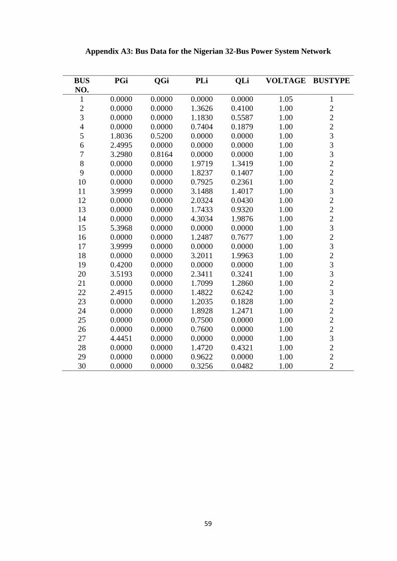
59
Appendix A3: Bus Data for the Nigerian 32-Bus Power System Network
BUS
NO.
PGi QGi PLi QLi VOLTAGE BUSTYPE
1 0.0000 0.0000 0.0000 0.0000 1.05 1
2 0.0000 0.0000 1.3626 0.4100 1.00 2
3 0.0000 0.0000 1.1830 0.5587 1.00 2
4 0.0000 0.0000 0.7404 0.1879 1.00 2
5 1.8036 0.5200 0.0000 0.0000 1.00 3
6 2.4995 0.0000 0.0000 0.0000 1.00 3
7 3.2980 0.8164 0.0000 0.0000 1.00 3
8 0.0000 0.0000 1.9719 1.3419 1.00 2
9 0.0000 0.0000 1.8237 0.1407 1.00 2
10 0.0000 0.0000 0.7925 0.2361 1.00 2
11 3.9999 0.0000 3.1488 1.4017 1.00 3
12 0.0000 0.0000 2.0324 0.0430 1.00 2
13 0.0000 0.0000 1.7433 0.9320 1.00 2
14 0.0000 0.0000 4.3034 1.9876 1.00 2
15 5.3968 0.0000 0.0000 0.0000 1.00 3
16 0.0000 0.0000 1.2487 0.7677 1.00 2
17 3.9999 0.0000 0.0000 0.0000 1.00 3
18 0.0000 0.0000 3.2011 1.9963 1.00 2
19 0.4200 0.0000 0.0000 0.0000 1.00 3
20 3.5193 0.0000 2.3411 0.3241 1.00 3
21 0.0000 0.0000 1.7099 1.2860 1.00 2
22 2.4915 0.0000 1.4822 0.6242 1.00 3
23 0.0000 0.0000 1.2035 0.1828 1.00 2
24 0.0000 0.0000 1.8928 1.2471 1.00 2
25 0.0000 0.0000 0.7500 0.0000 1.00 2
26 0.0000 0.0000 0.7600 0.0000 1.00 2
27 4.4451 0.0000 0.0000 0.0000 1.00 3
28 0.0000 0.0000 1.4720 0.4321 1.00 2
29 0.0000 0.0000 0.9622 0.0000 1.00 2
30 0.0000 0.0000 0.3256 0.0482 1.00 2
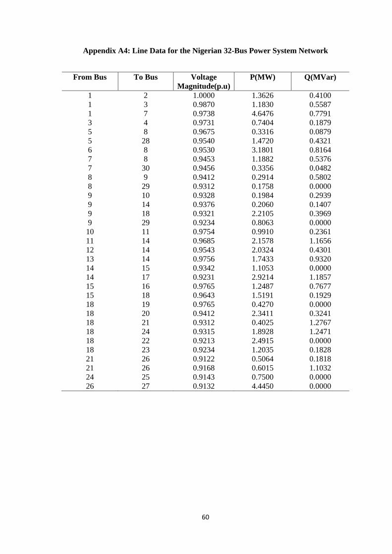
60
Appendix A4: Line Data for the Nigerian 32-Bus Power System Network
From Bus To Bus Voltage
Magnitude(p.u)
P(MW) Q(MVar)
1 2 1.0000 1.3626 0.4100
1 3 0.9870 1.1830 0.5587
1 7 0.9738 4.6476 0.7791
3 4 0.9731 0.7404 0.1879
5 8 0.9675 0.3316 0.0879
5 28 0.9540 1.4720 0.4321
6 8 0.9530 3.1801 0.8164
7 8 0.9453 1.1882 0.5376
7 30 0.9456 0.3356 0.0482
8 9 0.9412 0.2914 0.5802
8 29 0.9312 0.1758 0.0000
9 10 0.9328 0.1984 0.2939
9 14 0.9376 0.2060 0.1407
9 18 0.9321 2.2105 0.3969
9 29 0.9234 0.8063 0.0000
10 11 0.9754 0.9910 0.2361
11 14 0.9685 2.1578 1.1656
12 14 0.9543 2.0324 0.4301
13 14 0.9756 1.7433 0.9320
14 15 0.9342 1.1053 0.0000
14 17 0.9231 2.9214 1.1857
15 16 0.9765 1.2487 0.7677
15 18 0.9643 1.5191 0.1929
18 19 0.9765 0.4270 0.0000
18 20 0.9412 2.3411 0.3241
18 21 0.9312 0.4025 1.2767
18 24 0.9315 1.8928 1.2471
18 22 0.9213 2.4915 0.0000
18 23 0.9234 1.2035 0.1828
21 26 0.9122 0.5064 0.1818
21 26 0.9168 0.6015 1.1032
24 25 0.9143 0.7500 0.0000
26 27 0.9132 4.4450 0.0000

61
Appendix B1: m-File for Artificial Bee Colony
%Power Flow Code for Standard IEEE 14-bus Power System Network
% and the 32-bus Nigerian Power System Network
% Bukhari Tanko Rabiu ([email protected])
% MSc Student, Department of Electrical and Computer Engineering,
% Ahmadu Bello University Samaru-Zaria, Nigeria
% May, 2017.
%%%%%%%%%%%%%%%%%%%%%%%%%%%%%%%%%%%%%%%%%%%%%%%%%%%%%%%%%%%%%%%%%%%%%%
%%%%%%%%%%%%%%%%%%%%%%%%%%%%%%%%%%%%%%%%%%%%%%%%%%%%%%%%%%%%%%%%%%%%%%
function fFitness=calculateFitness(fObjV) fFitness=zeros(size(fObjV)); ind=find(fObjV>=0); fFitness(ind)=1./(fObjV(ind)+1); ind=find(fObjV<0); fFitness (ind)=1+abs(fObjV(ind));
function fm_call(flag)
%FM_CALL calls component equations % %FM_CALL(CASE) % CASE '1' algebraic equations % CASE 'pq' load algebraic equations % CASE '3' differential equations % CASE '1r' algebraic equations for Rosenbrock method % CASE '4' state Jacobians % CASE '0' initialization % CASE 'l' full set of equations and Jacobians % CASE 'kg' as "L" option but for distributed slack bus % CASE 'n' algebraic equations and Jacobians % CASE 'i' set initial point % CASE '5' non-windup limits % %see also FM_WCALL
fm_var
switch flag
case 'gen'
Line = gcall(Line); gcall(PQ) gcall(Shunt)
case 'load'
gcall(PQ) gcall(Shunt) gisland(Bus)
case 'gen0'
Line = gcall(Line); gcall(PQ) gcall(Shunt)
case 'load0'
62
gcall(PQ) gcall(Shunt) gisland(Bus)
case '3'
fcall(Syn)
case '1r'
Line = gcall(Line); gcall(PQ) gcall(Shunt) Syn = gcall(Syn); PV = gcall(PV); SW = gcall(SW); gisland(Bus)
case 'series'
Line = gcall(Line); gisland(Bus)
case '4'
DAE.Fx = sparse(DAE.n,DAE.n); DAE.Fy = sparse(DAE.n,DAE.m); DAE.Gx = sparse(DAE.m,DAE.n); Fxcall(Syn)
case '0'
Syn = setx0(Syn);
case 'fdpf'
Line = gcall(Line); gcall(PQ) gcall(Shunt) PV = gcall(PV); SW = gcall(SW); gisland(Bus)
case 'l'
Line = gcall(Line); gcall(PQ) gcall(Shunt) PV = gcall(PV); SW = gcall(SW); gisland(Bus) Gycall(Line) Gycall(PQ) Gycall(Shunt) Gycall(PV) Gycall(SW) Gyisland(Bus DAE.Fx = sparse(DAE.n,DAE.n); DAE.Fy = sparse(DAE.n,DAE.m);
63
DAE.Gx = sparse(DAE.m,DAE.n); Fxcall(PV) Fxcall(SW)
case 'kg'
Line = gcall(Line); gcall(PQ) gcall(Shunt) Syn = gcall(Syn); gisland(Bus) Gycall(Line) Gycall(PQ) Gycall(Shunt) Syn = Gycall(Syn); Gyisland(Bus)
fcall(Syn)
DAE.Fx = sparse(DAE.n,DAE.n); DAE.Fy = sparse(DAE.n,DAE.m); DAE.Gx = sparse(DAE.m,DAE.n); Fxcall(Syn)
case 'kgpf'
global PV SW Line = gcall(Line); gcall(PQ) gcall(Shunt) PV = gcall(PV); greactive(SW) glambda(SW,1,DAE.kg) gisland(Bus) Gycall(Line) Gycall(PQ) Gycall(Shunt) Gycall(PV) Gyreactive(SW) Gyisland(Bus)
DAE.Fx = sparse(DAE.n,DAE.n); DAE.Fy = sparse(DAE.n,DAE.m); DAE.Gx = sparse(DAE.m,DAE.n);
case 'n'
Line = gcall(Line); gcall(PQ) gcall(Shunt) Syn = gcall(Syn); PV = gcall(PV); SW = gcall(SW); gisland(Bus) Gycall(Line) Gycall(PQ) Gycall(Shunt) Syn = Gycall(Syn);
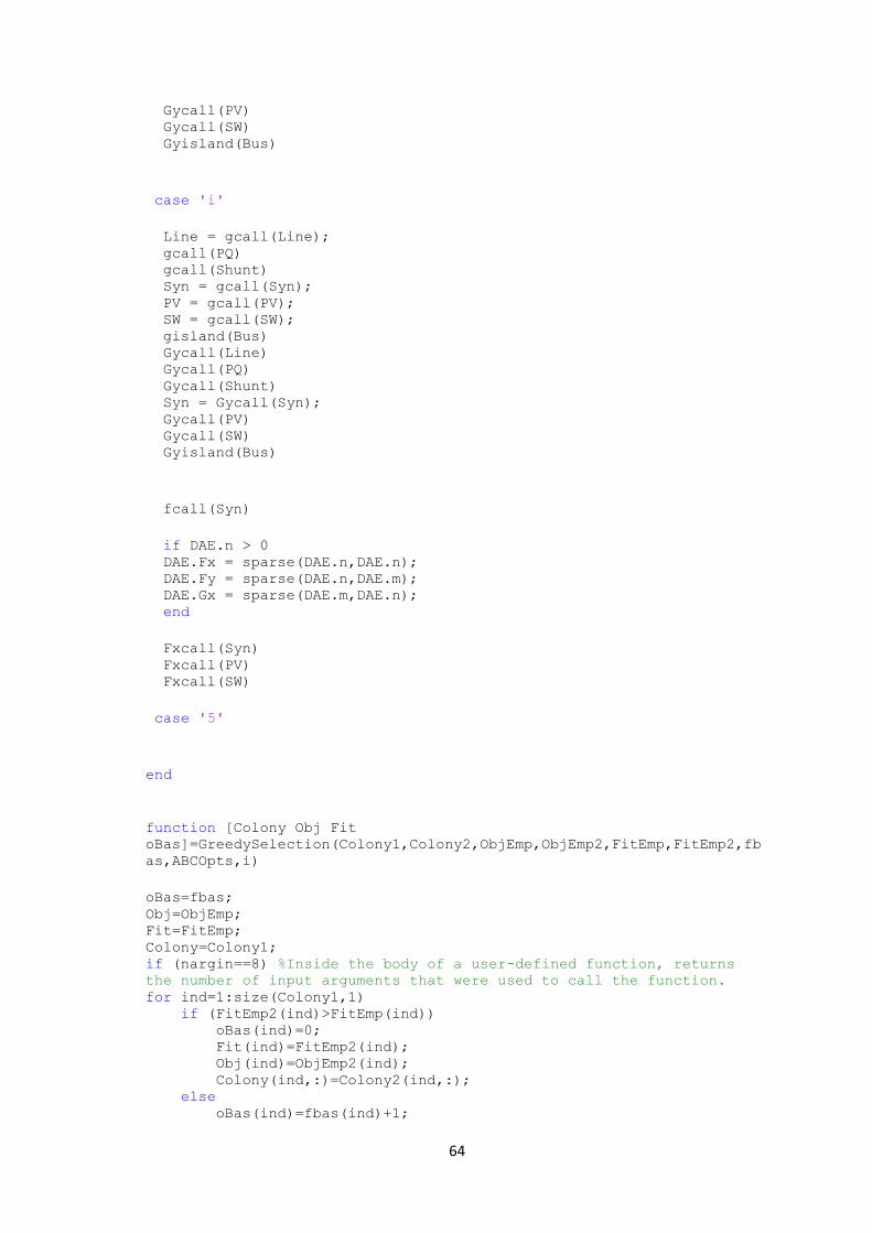
64
Gycall(PV) Gycall(SW) Gyisland(Bus)
case 'i'
Line = gcall(Line); gcall(PQ) gcall(Shunt) Syn = gcall(Syn); PV = gcall(PV); SW = gcall(SW); gisland(Bus) Gycall(Line) Gycall(PQ) Gycall(Shunt) Syn = Gycall(Syn); Gycall(PV) Gycall(SW) Gyisland(Bus)
fcall(Syn)
if DAE.n > 0 DAE.Fx = sparse(DAE.n,DAE.n); DAE.Fy = sparse(DAE.n,DAE.m); DAE.Gx = sparse(DAE.m,DAE.n); end
Fxcall(Syn) Fxcall(PV) Fxcall(SW)
case '5'
end
function [Colony Obj Fit
oBas]=GreedySelection(Colony1,Colony2,ObjEmp,ObjEmp2,FitEmp,FitEmp2,fb
as,ABCOpts,i)
oBas=fbas; Obj=ObjEmp; Fit=FitEmp; Colony=Colony1; if (nargin==8) %Inside the body of a user-defined function, returns
the number of input arguments that were used to call the function. for ind=1:size(Colony1,1) if (FitEmp2(ind)>FitEmp(ind)) oBas(ind)=0; Fit(ind)=FitEmp2(ind); Obj(ind)=ObjEmp2(ind); Colony(ind,:)=Colony2(ind,:); else oBas(ind)=fbas(ind)+1;
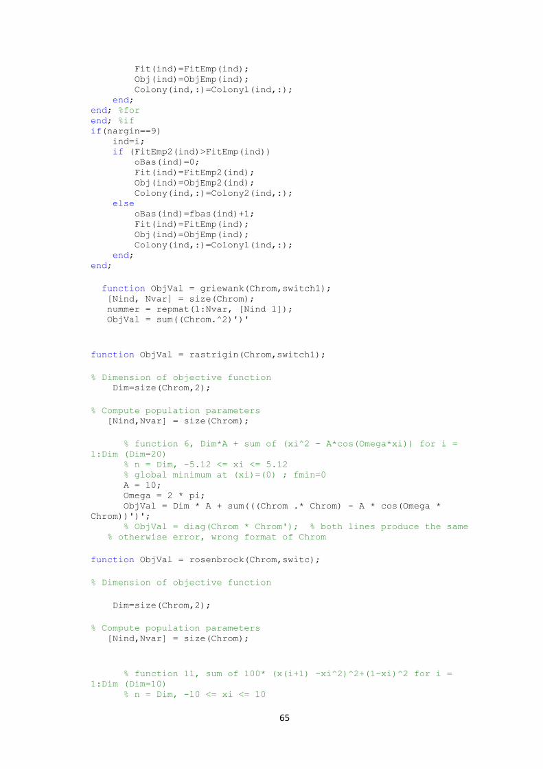
65
Fit(ind)=FitEmp(ind); Obj(ind)=ObjEmp(ind); Colony(ind,:)=Colony1(ind,:); end; end; %for end; %if if(nargin==9) ind=i; if (FitEmp2(ind)>FitEmp(ind)) oBas(ind)=0; Fit(ind)=FitEmp2(ind); Obj(ind)=ObjEmp2(ind); Colony(ind,:)=Colony2(ind,:); else oBas(ind)=fbas(ind)+1; Fit(ind)=FitEmp(ind); Obj(ind)=ObjEmp(ind); Colony(ind,:)=Colony1(ind,:); end; end;
function ObjVal = griewank(Chrom,switch1); [Nind, Nvar] = size(Chrom); nummer = repmat(1:Nvar, [Nind 1]); ObjVal = sum((Chrom.^2)')'
function ObjVal = rastrigin(Chrom,switch1);
% Dimension of objective function Dim=size(Chrom,2);
% Compute population parameters [Nind,Nvar] = size(Chrom);
% function 6, Dim*A + sum of (xi^2 - A*cos(Omega*xi)) for i =
1:Dim (Dim=20) % n = Dim, -5.12 <= xi <= 5.12 % global minimum at (xi)=(0) ; fmin=0 A = 10; Omega = 2 * pi; ObjVal = Dim * A + sum(((Chrom .* Chrom) - A * cos(Omega *
Chrom))')'; % ObjVal = diag(Chrom * Chrom'); % both lines produce the same % otherwise error, wrong format of Chrom
function ObjVal = rosenbrock(Chrom,switc);
% Dimension of objective function
Dim=size(Chrom,2);
% Compute population parameters [Nind,Nvar] = size(Chrom);
% function 11, sum of 100* (x(i+1) -xi^2)^2+(1-xi)^2 for i =
1:Dim (Dim=10) % n = Dim, -10 <= xi <= 10
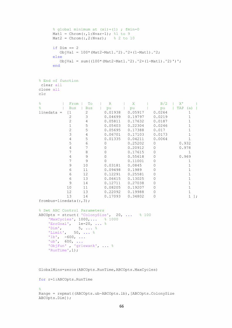
66
% global minimum at (xi)=(1) ; fmin=0 Mat1 = Chrom(:,1:Nvar-1); %1 to 9 Mat2 = Chrom(:,2:Nvar); % 2 to 10
if Dim == 2 ObjVal = 100*(Mat2-Mat1.^2).^2+(1-Mat1).^2; else ObjVal = sum((100*(Mat2-Mat1.^2).^2+(1-Mat1).^2)')'; end
% End of function clear all close all clc
% | From | To | R | X | B/2 | X' | % | Bus | Bus | pu | pu | pu | TAP (a) | linedata = [1 2 0.01938 0.05917 0.0264 1 2 3 0.04699 0.19797 0.0219 1 2 4 0.05811 0.17632 0.0187 1 1 5 0.05403 0.22304 0.0246 1 2 5 0.05695 0.17388 0.017 1 3 4 0.06701 0.17103 0.0173 1 4 5 0.01335 0.04211 0.0064 1 5 6 0 0.25202 0 0.932 4 7 0 0.20912 0 0.978 7 8 0 0.17615 0 1 4 9 0 0.55618 0 0.969 7 9 0 0.11001 0 1 9 10 0.03181 0.0845 0 1 6 11 0.09498 0.1989 0 1 6 12 0.12291 0.25581 0 1 6 13 0.06615 0.13025 0 1 9 14 0.12711 0.27038 0 1 10 11 0.08205 0.19207 0 1 12 13 0.22092 0.19988 0 1 13 14 0.17093 0.34802 0 1 ]; frombus=linedata(:,3);
% Set ABC Control Parameters ABCOpts = struct( 'ColonySize', 20, ... % 100 'MaxCycles', 1000,... % 1000 'ErrGoal', 1e-20, ... % 'Dim', 5, ... % 'Limit', 50, ... % 'lb', -600, ... 'ub', 600, ... 'ObjFun' , 'griewank', ... % 'RunTime',1);
GlobalMins=zeros(ABCOpts.RunTime,ABCOpts.MaxCycles)
for r=1:ABCOpts.RunTime
% Range = repmat((ABCOpts.ub-ABCOpts.lb),[ABCOpts.ColonySize
ABCOpts.Dim]);
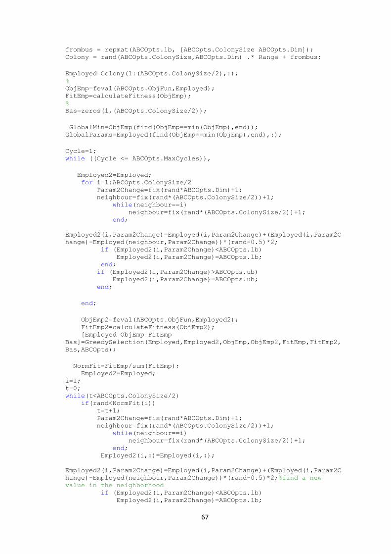
67
frombus = repmat(ABCOpts.lb, [ABCOpts.ColonySize ABCOpts.Dim]); Colony = rand(ABCOpts.ColonySize,ABCOpts.Dim) .* Range + frombus;
Employed=Colony(1:(ABCOpts.ColonySize/2),:); % ObjEmp=feval(ABCOpts.ObjFun,Employed); FitEmp=calculateFitness(ObjEmp); % Bas=zeros(1,(ABCOpts.ColonySize/2));
GlobalMin=ObjEmp(find(ObjEmp==min(ObjEmp),end)); GlobalParams=Employed(find(ObjEmp==min(ObjEmp),end),:);
Cycle=1; while ((Cycle <= ABCOpts.MaxCycles)),
Employed2=Employed; for i=1:ABCOpts.ColonySize/2 Param2Change=fix(rand*ABCOpts.Dim)+1; neighbour=fix(rand*(ABCOpts.ColonySize/2))+1; while(neighbour==i) neighbour=fix(rand*(ABCOpts.ColonySize/2))+1; end;
Employed2(i,Param2Change)=Employed(i,Param2Change)+(Employed(i,Param2C
hange)-Employed(neighbour,Param2Change))*(rand-0.5)*2; if (Employed2(i,Param2Change)<ABCOpts.lb) Employed2(i,Param2Change)=ABCOpts.lb; end; if (Employed2(i,Param2Change)>ABCOpts.ub) Employed2(i,Param2Change)=ABCOpts.ub; end;
end;
ObjEmp2=feval(ABCOpts.ObjFun,Employed2); FitEmp2=calculateFitness(ObjEmp2); [Employed ObjEmp FitEmp
Bas]=GreedySelection(Employed,Employed2,ObjEmp,ObjEmp2,FitEmp,FitEmp2,
Bas,ABCOpts);
NormFit=FitEmp/sum(FitEmp); Employed2=Employed; i=1; t=0; while(t<ABCOpts.ColonySize/2) if(rand<NormFit(i)) t=t+1; Param2Change=fix(rand*ABCOpts.Dim)+1; neighbour=fix(rand*(ABCOpts.ColonySize/2))+1; while(neighbour==i) neighbour=fix(rand*(ABCOpts.ColonySize/2))+1; end; Employed2(i,:)=Employed(i,:);
Employed2(i,Param2Change)=Employed(i,Param2Change)+(Employed(i,Param2C
hange)-Employed(neighbour,Param2Change))*(rand-0.5)*2;%find a new
value in the neighborhood if (Employed2(i,Param2Change)<ABCOpts.lb) Employed2(i,Param2Change)=ABCOpts.lb;
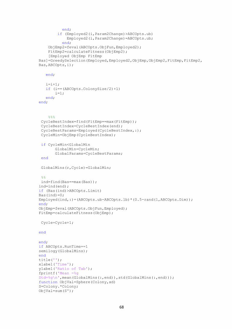
68
end; if (Employed2(i,Param2Change)>ABCOpts.ub) Employed2(i,Param2Change)=ABCOpts.ub; end; ObjEmp2=feval(ABCOpts.ObjFun,Employed2); FitEmp2=calculateFitness(ObjEmp2); [Employed ObjEmp FitEmp
Bas]=GreedySelection(Employed,Employed2,ObjEmp,ObjEmp2,FitEmp,FitEmp2,
Bas,ABCOpts,i);
end;
i=i+1; if (i==(ABCOpts.ColonySize/2)+1) i=1; end; end;
%%% CycleBestIndex=find(FitEmp==max(FitEmp)); CycleBestIndex=CycleBestIndex(end); CycleBestParams=Employed(CycleBestIndex,:); CycleMin=ObjEmp(CycleBestIndex);
if CycleMin<GlobalMin GlobalMin=CycleMin; GlobalParams=CycleBestParams; end
GlobalMins(r,Cycle)=GlobalMin;
%% ind=find(Bas==max(Bas)); ind=ind(end); if (Bas(ind)>ABCOpts.Limit) Bas(ind)=0; Employed(ind,:)=(ABCOpts.ub-ABCOpts.lb)*(0.5-rand(1,ABCOpts.Dim)); end; ObjEmp=feval(ABCOpts.ObjFun,Employed); FitEmp=calculateFitness(ObjEmp);
Cycle=Cycle+1;
end
end; if ABCOpts.RunTime==1 semilogy(GlobalMins); end title(''); xlabel('Time'); ylabel('Ratio of Tab'); fprintf('Mean =%g
Std=%g\n',mean(GlobalMins(:,end)),std(GlobalMins(:,end))); function ObjVal=Sphere(Colony,xd) S=Colony.*Colony; ObjVal=sum(S');
69
function appfre s = tf('s'); R = 10; % resistor
resistance Req = 40; % inductor
equivalent series resistance (ESR) L = 1; % inductor
inductance C = 510*10^-6; % capacitor
capacitance ei = 1.53; % battery
voltage tstep = 1.22; % time step
occurred G = 1/(C*L*s^2 + C*(R+Req)*s + 1); % model transfer
function [y,t] = step(G*ei,0.5); % model step
response with battery voltage scaling plot(t,y) hold plot(eo.Time(100*tstep:100*tstep+50)-
tstep,eo.Data(100*tstep:100*tstep+50),'r:') % experimental data xlabel('time (sec)') ylabel('output voltage (Volts)') title('LRC Circuit Step Response') legend('model','experiment','Location','SouthEast') s = tf('s'); R = 10000; % resistance of
resistor in RC circuit C = 100*10^-6; % capacitance of
capacitor in RC circuit G = 1/(C*R*s+1); % RC circuit
transfer function step (G) title('RC Circuit Step Response (R = 10 kOhm, C = 100 uF)')
%%%%%%%%%%%%%%%%%%%%%%%%%%%%%%%%%%%%%%%%%%%%%%%%%%%%%%%%%%%%%%%%%%%%%%
% m-file for Bacterial Foraging Algorithm (BFA)
% --------------------------------------------------------------------
% (1) Initialization
p = 2; % Dimension of search space
S = 10; % Number of bacteria in the colony
Nc = 4; % Number of chemotactic steps
Ns = 4; % Number of swim steps
Nre= 4; % Number of reproductive steps
Ned= 3; % Number of elimination and dispersal steps
Sr =S/2;% The number of bacteria reproductions (splits) per generation
Ped=0.25; % The probability that each bacteria will be
eliminated/dispersed
n = 14;
ca(:,1)=0.01*ones(S,1); % the run length unit (the size of the step
taken in each run or tumble)
% Initial positions
for m=1:S % the initial positions
B(1,:,1,1,1)= 2 + (n-2)*rand(S,1)';
B(2,:,1,1,1)= 0.5 + (2-0.5)*rand(S,1)';
%format short,B(2,:,1,1,1);
end
%% Loops
% (2) Elimination-dispersal loop
for l = 1:Ned
70
% (3) Reproduction loop
for k = 1:Nre
% (4) Chemotaxis (swim/tumble) loop
for j=1:Nc
% (4.1) Chemotactic step
for i=1:S
% (4.2a) Fitness function
J(i,j,k,l) = fitnessIBFADSS33(B(:,i,j,k,l));
% (4.2b) Add on cell-to-cell attraction effect
J(i,j,k,l)=J(i,j,k,l)+cell_to_cell_func(B(:,i,j,k,l),B(:,:,j,k,l),S);
% (4.3) Jlast
Jlast=J(i,j,k,l);
% (4.4) Tumble
Delta(:,i) = unifrnd(-1,1,p,1);
% (4.5) Move
B(:,i,j+1,k,l)=B(:,i,j,k,l)+ca(i,k)*Delta(:,i)/sqrt(Delta(:,i)'*Delta(
:,i)); % with the original run length unit
%
B(:,i,j+1,k,l)=B(:,i,j,k,l)+(ca(i,k)/(1+(1/(0.01*(abs(J(i,j,k,l)))))))
*Delta(:,i)/sqrt(Delta(:,i)'*Delta(:,i)); % with linear adaptive run
length unit
%
B(:,i,j+1,k,l)=B(:,i,j,k,l)+(ca(i,k)/(1+(1/(0.01*(((abs(J(i,j,k,l)))^2
) + (abs(J(i,j,k,l))))))))*Delta(:,i)/sqrt(Delta(:,i)'*Delta(:,i)); %
with quadratic adaptive run length unit
%
B(:,i,j+1,k,l)=B(:,i,j,k,l)+(ca(i,k)/(1+(1/(0.01*(exp(abs(J(i,j,k,l)))
)))))*Delta(:,i)/sqrt(Delta(:,i)'*Delta(:,i)); % with exponential
adaptive run length unit
% (4.6a) New fitness function
J(i,j+1,k,l)= fitnessIBFADSS33(B(:,i,j+1,k,l));
% 4.6b) Add on cell-to-cell attraction effect
J(i,j+1,k,l)=J(i,j+1,k,l)+cell_to_cell_func(B(:,i,j+1,k,l),B(:,:,j+1,k
,l),S);
if J(i,j+1,k,l)<Jlast
Jlast=J(i,j+1,k,l);
B(:,i,j+1,k,l)=B(:,i,j+1,k,l)+ca(i,k)*Delta(:,i)/sqrt(Delta(:,i)'*Delt
a(:,i)) ;
J(i,j+1,k,l)= fitnessBFADSS33(B(:,i,j+1,k,l));
else
m=Ns;
end
end
J(i,j,k,l)=Jlast; %???
end % (4.8) Next bacterium
OPTIMUM_BUS = B(1,:,j,k,l);
Q OLTC = B(2,:,j,k,l);
%format short,Q_OLTC;
% if OPTIMUM_BUS <=1;
% OPTIMUM_BUS = round((abs(OPTIMUM_BUS))+1);
% end
end % (5) if j < Nc, chemotaxis
% (6) Reproduction
% (6.1) Health
Jhealth=sum(J(:,:,k,l),2); % Set the health of each of the S bacteria
[Jhealth,sortind]=sort(Jhealth);% Sorts bacteria in order of ascending
values
B(:,:,1,k+1,l)=B(:,sortind,Nc+1,k,l);

71
ca(:,k+1)=ca(sortind,k); % Keeps the chemotaxis parameters with each
bacterium at the next generation
% (6.2) Split the bacteria
for i=1:Sr % Sr??
B(:,i+Sr,1,k+1,l)=B(:,i,1,k+1,l); % The least fit do not reproduce,
the most fit ones split into two identical copies
ca(i+Sr,k+1)=ca(i,k+1);
end
end % (7) Loop to go to the next reproductive step
% (8) Elimination-dispersal
for m=1:S
if Ped>rand % % Generate random number
B(1,:,1,1,1)= 2 + (n-2)*rand(S,1)';
B(2,:,1,1,1)= 0.5 + (10-0.5)*rand(S,1)';
%format short,B(2,:,1,1,1);
else
B(:,m,1,1,l+1)=B(:,m,1,Nre+1,l); % Bacteria that are not dispersed
end
end
end
%% Results
reproduction = J(:,1:Nc,Nre,Ned);
[jlastreproduction,O] = min(reproduction,[],2); % min cost function
for each bacterial
[Y,I] = min(jlastreproduction);
OPTIMUM_BUS = round(pbest(1,:));% Return the optimal positions as Kp
and Kd
Q_OLTC = pbest(2,:);
%%%%%%%%%%%%%%%%%% End of BFA Code %%%%%%%%%%%%%%%%%%%%%%%%%%%%%%%%%%
%%%%%%%%%%%%%%%%%%%%%%%%%%%%%%%%%%%%%%%%%%%%%%%%%%%%%%%%%%%%%%%%%%%%%%
%%%%%%%%%%%%%%%%%%%%%%%%%%%%%%%%%%%%%%%%%%%%%%%%%%%%%%%%%%%%%%%%%%%%%%


![Evolution of sustained foraging in three-dimensional ... · concepts are the bacterial foraging optimization algorithm (BFOA) [18], and artificial bee colony (ABC)[19]. Information](https://img.pdfslide.us/doc/110x75/602f7045505a0833176355a6/evolution-of-sustained-foraging-in-three-dimensional-concepts-are-the-bacterial.jpg)