Natural selection tends to eliminate animalswith poor “foraging strategies” (methodsfor locating, handling, and ingesting food)and favor the propagation of genes of thoseanimals that have successful foragingstrategies since they are more likely to en-

joy reproductive success (they obtain enough food to en-able them to reproduce). After many generations, poorforaging strategies are either eliminated or shaped intogood ones (redesigned). Logically, such evolutionary princi-ples have led scientists in the field of “foraging theory” tohypothesize that it is appropriate to model the activity offoraging as an optimization process: A foraging animal takesactions to maximize the energy obtained per unit time spentforaging, in the face of constraints presented by its ownphysiology (e.g., sensing and cognitive capabilities) and en-vironment (e.g., density of prey, risks from predators, physi-cal characteristics of the search area). Evolution hasbalanced these constraints and essentially “engineered”

what is sometimes referred to as an “optimal foraging pol-icy” (such terminology is especially justified in cases wherethe models and policies have been ecologically validated).Optimization models are also valid for “social foraging”where groups of animals cooperatively forage.

Here, we explain the biology and physics underlying thechemotactic (foraging) behavior of E. coli bacteria (yes, theones that are living in your intestines). We explain a varietyof bacterial swarming and social foraging behaviors and dis-cuss the control system on the E. coli that dictates how for-aging should proceed. Next, a computer program thatemulates the distributed optimization process representedby the activity of social bacterial foraging is presented. To il-lustrate its operation, we apply it to a simple multi-ple-extremum function minimization problem and brieflydiscuss its relationship to some existing optimization algo-rithms. The article closes with a brief discussion on the po-tential uses of biomimicry of social foraging to developadaptive controllers and cooperative control strategies forautonomous vehicles. For this, we provide some basic ideasand invite the reader to explore the concepts further. Hence,this article should be thought of as an introduction to someinteresting biological phenomena that suggest new types of

52 IEEE Control Systems Magazine June 20020272-1708/02/$17.00©2002IEEE

The author (passino@ee.eng.ohio-state.edu) is with the Departmentof Electrical Engineering, The Ohio State University, 2015 Neil Ave-nue, Columbus, OH 43210-1272, U.S.A.

optimization methods; the relevance to control systemsneeds to be further investigated, and thorough compari-sons to the vast literature on global optimization remain tobe done.

ForagingElements of Foraging TheoryForaging theory is based on the assumption that animalssearch for and obtain nutrients in a way that maximizestheir energy intake E per unit time T spent foraging. Hence,they try to maximize a function like

ET

(or they maximize their long-term average rate of energy in-take). Maximization of such a function provides nutrientsources to survive and additional time for other importantactivities (e.g., fighting, fleeing, mating, reproducing, sleep-ing, or shelter building). Shelter-building and mate-findingactivities sometimes bear similarities to foraging. Clearly,foraging is very different for different species. Herbivoresgenerally find food easily but must eat a lot of it. Carnivoresgenerally find it difficult to locate food but do not have to eatas much since their food is of high energy value. The “envi-ronment” establishes the pattern of nutrients that are avail-able (e.g., via what other organisms are nutrients available,geological constraints such as rivers and mountains, andweather patterns), and it places constraints on obtainingthat food (e.g., small portions of food may be separated bylarge distances). During foraging there can be risks due topredators, the prey may be mobile so it must be chased, andthe physiological characteristics of the forager constrain itscapabilities and ultimate success.

For many animals, nutrients are distributed in “patches”(e.g., a lake, a meadow, a bush with berries, a group of treeswith fruit). Foraging involves finding such patches, decidingwhether to enter a patch and search for food, and whetherto continue searching for food in the current patch or to gofind another patch that hopefully has a higher quality andquantity of nutrients than the current patch. Patches aregenerally encountered sequentially, and sometimes great ef-fort and risk are needed to travel from one patch to another.Generally, if an animal encounters a nutrient-poor patch,but based on past experience it expects that there should bea better patch elsewhere, then it will consider risks and ef-forts to find another patch, and if it finds them acceptable, itwill seek another patch. Also, if an animal has been in apatch for some time, it can begin to deplete its resources, sothere should be an optimal time to leave the patch and ven-ture out to try to find a richer one. It does not want to wasteresources that are readily available, but it also does notwant to waste time in the face of diminishing energy returns.

Optimal foraging theory formulates the foraging problemas an optimization problem and via computational or ana-

lytical methods can provide an optimal foraging “policy”that specifies how foraging decisions are made (tradition-ally, dynamic programming formulations have been used[1]). There are quantifications of what foraging decisionsmust be made, measures of currency (the opposite of cost),and constraints on the parameters of the optimization. Forinstance, researchers have studied how to maximizelong-term average rate of energy intake where only certaindecisions and constraints are allowed. Constraints due toincomplete information (e.g., due to limited sensing capabil-ities) and risks (e.g., due to predators) have been consid-ered. Essentially, these optimization approaches seek toconstruct an optimal controller (policy) for making foragingdecisions. Some biologists have questioned the validity ofsuch an approach, arguing that no animal can make optimaldecisions (see the references in [1]). However, the optimalforaging formulation is only meant to be a model that ex-plains what optimal behavior would be like. In fact, some re-searchers have shown that foraging decision heuristics areused very effectively by animals to approximate optimalpolicies, given the physiological (and other) constraintsthat are imposed on the animal [1].

Search Strategies for ForagingIn one approach to the study of foraging search strategies[2], predation is broken into components that are similar formany animals. First, predators must search for and locateprey. Next, they pursue and attack the prey. Finally, they“handle” and ingest the prey. The importance of variouscomponents of foraging behavior depends on the relation-ship between the predator and the prey. If the prey is largerthan the predator, then the pursuit, attack, and handling canbe most important. The prey may be easy to find, but theprey’s size gives it an advantage. If the prey is smaller thanthe predator, then generally the search component of forag-ing is most important. Small size can be an advantage for theprey. Since prey are often smaller than predators for manyanimals, they must be consumed often and in large num-bers; this makes the search time limit other components ofthe predation cycle. In this article, we consider cases wherethe searching behavior is the dominant factor in foraging.This is the case for many birds, fish, lizards, and insects.

Some animals are “cruise” or “ambush” searchers. Forthe cruise approach to searching, the forager moves contin-uously through the environment, constantly searching forprey at the boundary of the volume being searched (tunafish and hawks are cruise searchers). In ambush search, theforager (e.g., a rattlesnake) remains stationary and waits forprey to cross into its strike range. The search strategies ofmany species are actually between the cruise and ambushextremes. In particular, in “saltatory search” strategies, ananimal will intermittently cruise and sit and wait, possiblychanging direction at various times when it stops and possi-bly while it moves. To envision this strategy, consider Fig. 1,where distance traveled in searching is plotted versus time.

June 2002 IEEE Control Systems Magazine 53

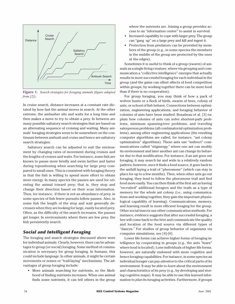
In cruise search, distance increases at a constant rate dic-tated by how fast the animal moves in search. At the otherextreme, the ambusher sits and waits for a long time andthen makes a move to try to obtain a prey. In between aremany possible saltatory search strategies that are based onan alternating sequence of cruising and waiting. Many ani-mals’ foraging strategies seem to lie somewhere on the con-tinuum between ambush and cruise and hence are saltatorysearch strategies.

Saltatory search can be adjusted to suit the environ-ment by changing rates of movement during cruises andthe lengths of cruises and waits. For instance, some fish areknown to pause more briefly and swim farther and fasterduring repositioning when searching for large prey com-pared to small ones. This is consistent with foraging theoryin that the fish is willing to spend more effort to obtainmore energy. In many species the pauses are used for ori-enting the animal toward prey; that is, they stop andchange their direction based on their scan information.Then, for instance, if there is not an abundance of prey, insome species of fish fewer pursuits follow pauses. Also, insome fish the length of the stop and wait generally de-creases when they are looking for large, easily located prey.Often, as the difficulty of the search increases, the pausesget longer. In environments where there are few prey, thefish persistently search.

Social and Intelligent ForagingThe foraging and search strategies discussed above werefor individual animals. Clearly, however, there can be advan-tages to group (or social) foraging. Some method of commu-nication is necessary for group foraging. In humans, thiscould include language. In other animals, it might be certainmovements or noises or “trail-laying” mechanisms. The ad-vantages of group foraging include:

• More animals searching for nutrients, so the likeli-hood of finding nutrients increases. When one animalfinds some nutrients, it can tell others in the group

where the nutrients are. Joining a group provides ac-cess to an “information center” to assist in survival.

• Increased capability to cope with larger prey. The groupcan “gang up” on a large prey and kill and ingest it.

• Protection from predators can be provided by mem-bers of the group (e.g., in some species the membersin the middle of the group are protected by the onesat the edges).

Sometimes it is useful to think of a group (swarm) of ani-mals as a single living creature, where via grouping and com-munication a “collective intelligence” emerges that actuallyresults in more successful foraging for each individual in thegroup (and the gains can offset effects of food competitionwithin groups; by working together there can be more foodthan if there is no cooperation).

For group foraging, you may think of how a pack ofwolves hunts or a flock of birds, swarm of bees, colony ofants, or school of fish behave. Connections between optimi-zation, engineering applications, and foraging behavior ofcolonies of ants have been studied. Bonabeau et al. [3] ex-plain how colonies of ants can solve shortest-path prob-lems, minimum spanning-tree problems, and travelingsalesperson problems (all combinatorial optimization prob-lems), among other engineering applications (the resultingcomputer algorithms are called, for instance, “ant colonyoptimization” algorithms). These ants use “indirect” com-munications called “stigmergy,” where one ant can modifyits environment and later another ant can change its behav-ior due to that modification. For instance, if an ant goes outforaging, it may search far and wide in a relatively randompattern; however, once it finds a food source, it goes back tothe anthill laying a trail of “pheromone” (which can stay inplace for up to a few months). Then, when other ants go outforaging, they tend to follow the pheromone trail and findfood more easily. You can then think of the first ant as having“recruited” additional foragers and the trails as a type ofmemory for the whole ant colony (i.e., using communica-tions and working together, they gain the important physio-logical capability of learning). Communications, memory,and learning result in more efficient foraging for the group.Other social insects use other communication methods. Forinstance, evidence suggests that after successful foraging, abee will come back to the hive and communicate the qualityand location of the food source via different types of“dances.” For studies of group behavior of organisms viacomputer simulations, see [4]-[6].

Lower life forms can achieve higher forms of foraging in-telligence by cooperating in groups (e.g., the ants “learn”where food is located). Lone individuals of higher life forms,however, are naturally endowed with more cognitive andhence foraging capabilities. For instance, in some species anindividual forager can pay attention to the critical parts of itsenvironment. It may be able to learn about the environmentand characteristics of its prey (e.g., by developing and stor-ing cognitive maps). It may be able to use this learned infor-mation to plan its foraging activities. Furthermore, if groups

54 IEEE Control Systems Magazine June 2002

Distance

CruiseSearch

SaltatorySearch

Ambush Search

Time

Figure 1. Search strategies for foraging animals (figure adaptedfrom [2]).

of foragers can learn and plan their activities, it is possiblefor even greater success to be obtained. Indeed, it seemsthat humans often act as group foragers that can collec-tively learn and plan. Of course, humans are significantly dif-ferent from many life forms since, rather than simply tryingto cope with a given foraging environment, we focus onmodifying our environment via farming to improve our for-aging success.

In the next section, we will consider individual and groupforaging for bacteria, organisms that are much simpler thanants or humans yet can still work together for the benefit ofthe group. You may think of these as tiny autonomous vehi-cles or as executing a simple yet effective optimization pro-cess during foraging, one that may be useful in the solutionto control problems. Or you may simply be interested in theunderlying control science (e.g., what type of control algo-rithm operates to implement their foraging strategy). Afterexplaining how bacteria forage, we will model them via acomputer simulation and then briefly discuss their rele-vance to adaptive control and cooperative control for au-tonomous vehicles.

Bacterial Foraging: E. coliThe E. coli bacterium has a plasma membrane, cell wall,and capsule that contains the cytoplasm and nucleoid. Thepili (singular, pilus) are used for a type of gene transfer toother E. coli bacteria, and flagella (singular, flagellum) areused for locomotion. The cell is about 1 µm in diameter and2 µm in length. The E. coli cell only weighs about 1picogram and is about 70% water. Salmonella typhimuriumis a similar type of bacterium.

The E. coli bacterium is probably the best understood mi-croorganism. Its entire genome has been sequenced; it con-tains 4,639,221 of the A, C, G, and T “letters”—adenosine,cytosine, guanine, and thymine—arranged into a total of4,288 genes. Mutations in E. coli occur at a rate of about 10−7

per gene, per generation, and can affect its physiological as-pects (e.g., reproductive efficiency at different tempera-tures). E. coli bacteria occasionally engage in a type of “sex”called “conjugation” where small gene sequences areunidirectionally transferred from one bacterium to anothervia an extended pilus.

When E. coli grows, it gets longer, then divides in the mid-dle into two “daughters.” Given sufficient food and held atthe temperature of the human gut (one place where theylive) of 37 ° C, E. coli can synthesize and replicate everythingit needs to make a copy of itself in about 20 min; hencegrowth of a population of bacteria is exponential with a rela-tively short time to double. For instance, following [8], if atnoon today you start with one cell and sufficient food, bynoon tomorrow there will be 2 4 7 1072 21= ×. cells, which isenough to pack a cube 17 m on one side (it should be clearthat with enough food, at this reproduction rate, they couldquickly cover the entire earth with a knee-deep layer!).

The E. coli bacterium has a control system (guidance sys-tem) that enables it to search for food and try to avoid nox-ious substances. For instance, it swims away from alkalineand acidic environments and toward more neutral ones. Toexplain the behavior of the E. coli bacterium, we will explainits actuator (the flagellum), “decision making,” sensors, andclosed-loop behavior (i.e., how it moves in various environ-ments—its motile behavior). You will see that E. coli per-forms a type of saltatory search. This section is based on thework in [7]-[15].

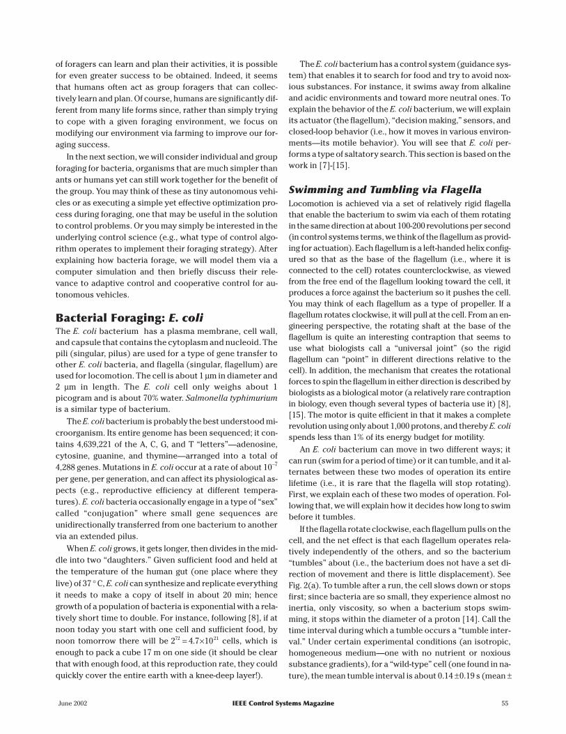
Swimming and Tumbling via FlagellaLocomotion is achieved via a set of relatively rigid flagellathat enable the bacterium to swim via each of them rotatingin the same direction at about 100-200 revolutions per second(in control systems terms, we think of the flagellum as provid-ing for actuation). Each flagellum is a left-handed helix config-ured so that as the base of the flagellum (i.e., where it isconnected to the cell) rotates counterclockwise, as viewedfrom the free end of the flagellum looking toward the cell, itproduces a force against the bacterium so it pushes the cell.You may think of each flagellum as a type of propeller. If aflagellum rotates clockwise, it will pull at the cell. From an en-gineering perspective, the rotating shaft at the base of theflagellum is quite an interesting contraption that seems touse what biologists call a “universal joint” (so the rigidflagellum can “point” in different directions relative to thecell). In addition, the mechanism that creates the rotationalforces to spin the flagellum in either direction is described bybiologists as a biological motor (a relatively rare contraptionin biology, even though several types of bacteria use it) [8],[15]. The motor is quite efficient in that it makes a completerevolution using only about 1,000 protons, and thereby E. colispends less than 1% of its energy budget for motility.

An E. coli bacterium can move in two different ways; itcan run (swim for a period of time) or it can tumble, and it al-ternates between these two modes of operation its entirelifetime (i.e., it is rare that the flagella will stop rotating).First, we explain each of these two modes of operation. Fol-lowing that, we will explain how it decides how long to swimbefore it tumbles.

If the flagella rotate clockwise, each flagellum pulls on thecell, and the net effect is that each flagellum operates rela-tively independently of the others, and so the bacterium“tumbles” about (i.e., the bacterium does not have a set di-rection of movement and there is little displacement). SeeFig. 2(a). To tumble after a run, the cell slows down or stopsfirst; since bacteria are so small, they experience almost noinertia, only viscosity, so when a bacterium stops swim-ming, it stops within the diameter of a proton [14]. Call thetime interval during which a tumble occurs a “tumble inter-val.” Under certain experimental conditions (an isotropic,homogeneous medium—one with no nutrient or noxioussubstance gradients), for a “wild-type” cell (one found in na-ture), the mean tumble interval is about 0.14 ±0.19 s (mean ±

June 2002 IEEE Control Systems Magazine 55

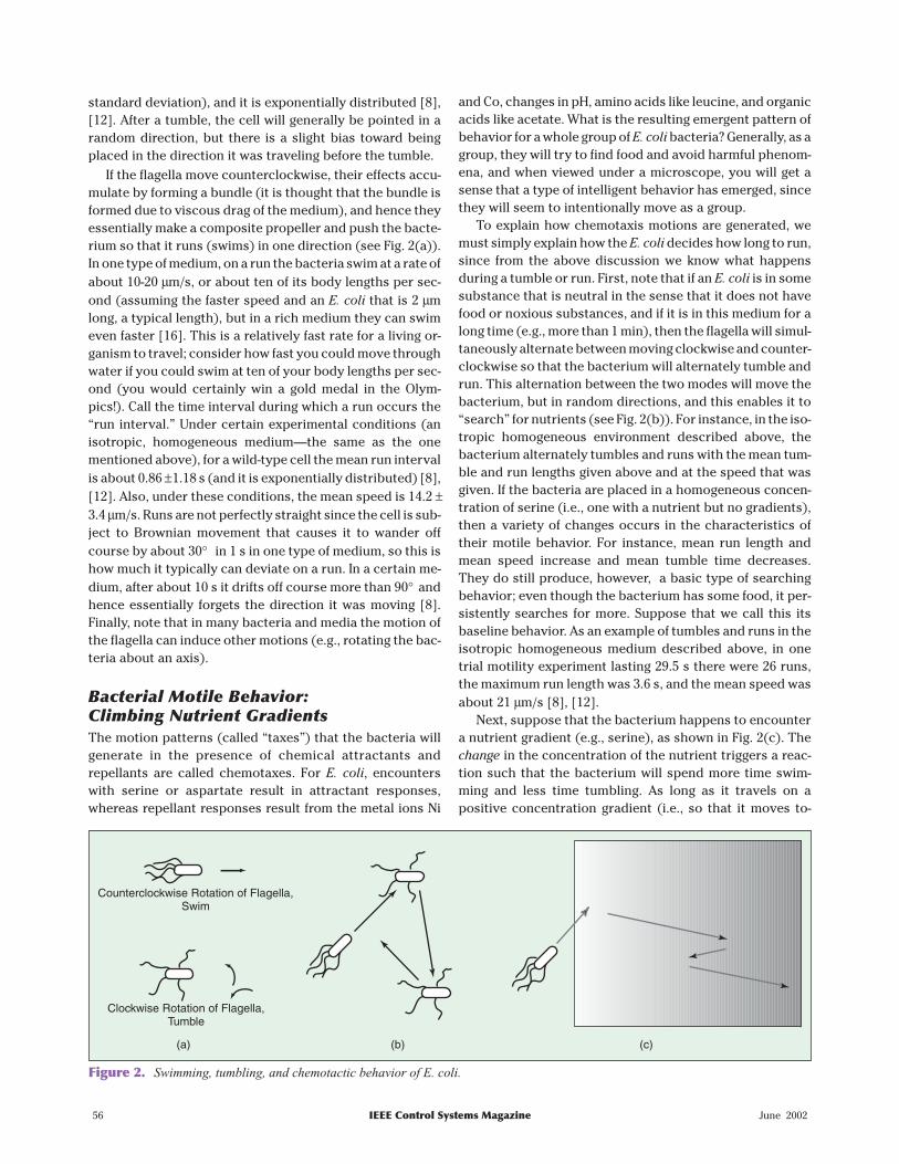
standard deviation), and it is exponentially distributed [8],[12]. After a tumble, the cell will generally be pointed in arandom direction, but there is a slight bias toward beingplaced in the direction it was traveling before the tumble.

If the flagella move counterclockwise, their effects accu-mulate by forming a bundle (it is thought that the bundle isformed due to viscous drag of the medium), and hence theyessentially make a composite propeller and push the bacte-rium so that it runs (swims) in one direction (see Fig. 2(a)).In one type of medium, on a run the bacteria swim at a rate ofabout 10-20 µm/s, or about ten of its body lengths per sec-ond (assuming the faster speed and an E. coli that is 2 µmlong, a typical length), but in a rich medium they can swimeven faster [16]. This is a relatively fast rate for a living or-ganism to travel; consider how fast you could move throughwater if you could swim at ten of your body lengths per sec-ond (you would certainly win a gold medal in the Olym-pics!). Call the time interval during which a run occurs the“run interval.” Under certain experimental conditions (anisotropic, homogeneous medium—the same as the onementioned above), for a wild-type cell the mean run intervalis about 0.86 ±1.18 s (and it is exponentially distributed) [8],[12]. Also, under these conditions, the mean speed is 14.2 ±3.4 µm/s. Runs are not perfectly straight since the cell is sub-ject to Brownian movement that causes it to wander offcourse by about 30° in 1 s in one type of medium, so this ishow much it typically can deviate on a run. In a certain me-dium, after about 10 s it drifts off course more than 90° andhence essentially forgets the direction it was moving [8].Finally, note that in many bacteria and media the motion ofthe flagella can induce other motions (e.g., rotating the bac-teria about an axis).

Bacterial Motile Behavior:Climbing Nutrient GradientsThe motion patterns (called “taxes”) that the bacteria willgenerate in the presence of chemical attractants andrepellants are called chemotaxes. For E. coli, encounterswith serine or aspartate result in attractant responses,whereas repellant responses result from the metal ions Ni

and Co, changes in pH, amino acids like leucine, and organicacids like acetate. What is the resulting emergent pattern ofbehavior for a whole group of E. coli bacteria? Generally, as agroup, they will try to find food and avoid harmful phenom-ena, and when viewed under a microscope, you will get asense that a type of intelligent behavior has emerged, sincethey will seem to intentionally move as a group.

To explain how chemotaxis motions are generated, wemust simply explain how the E. coli decides how long to run,since from the above discussion we know what happensduring a tumble or run. First, note that if an E. coli is in somesubstance that is neutral in the sense that it does not havefood or noxious substances, and if it is in this medium for along time (e.g., more than 1 min), then the flagella will simul-taneously alternate between moving clockwise and counter-clockwise so that the bacterium will alternately tumble andrun. This alternation between the two modes will move thebacterium, but in random directions, and this enables it to“search” for nutrients (see Fig. 2(b)). For instance, in the iso-tropic homogeneous environment described above, thebacterium alternately tumbles and runs with the mean tum-ble and run lengths given above and at the speed that wasgiven. If the bacteria are placed in a homogeneous concen-tration of serine (i.e., one with a nutrient but no gradients),then a variety of changes occurs in the characteristics oftheir motile behavior. For instance, mean run length andmean speed increase and mean tumble time decreases.They do still produce, however, a basic type of searchingbehavior; even though the bacterium has some food, it per-sistently searches for more. Suppose that we call this itsbaseline behavior. As an example of tumbles and runs in theisotropic homogeneous medium described above, in onetrial motility experiment lasting 29.5 s there were 26 runs,the maximum run length was 3.6 s, and the mean speed wasabout 21 µm/s [8], [12].

Next, suppose that the bacterium happens to encountera nutrient gradient (e.g., serine), as shown in Fig. 2(c). Thechange in the concentration of the nutrient triggers a reac-tion such that the bacterium will spend more time swim-ming and less time tumbling. As long as it travels on apositive concentration gradient (i.e., so that it moves to-

56 IEEE Control Systems Magazine June 2002

Clockwise Rotation of Flagella,Tumble

Counterclockwise Rotation of Flagella,Swim

(a) (b) (c)

Figure 2. Swimming, tumbling, and chemotactic behavior of E. coli.

ward increasing nutrient concentrations)it will tend to lengthen the time it spendsswimming (i.e., it runs farther), up to apoint. The directions of movement are “bi-ased” toward increasing nutrient gradi-ents. The cell does not change its directionon a run due to changes in the gradient—the tumbles basically determine the direc-tion of the run, aside from the Brownian in-fluences mentioned above.

On the other hand, typically if the bacte-rium happens to swim down a concentra-tion gradient (or into a positive gradient ofnoxious substances), it will return to itsbaseline behavior so that essentially it tries to search for away to climb back up the gradient (or down the noxious sub-stance gradient). For instance, under certain conditions, fora wild-type cell swimming up serine gradients, the mean runlength is 2.19 ±3.43 s, but if it swims down a serine gradientthe mean run length is 1.40 ± 1.88 s [12]. Hence, when itmoves up the gradient, it lengthens its runs. The mean runlength for swimming down the gradient is the one that is ex-pected considering that the bacteria are in this particulartype of medium; they act basically the same as in a homoge-neous medium, so that they are engaging their search/avoidance behavior (baseline behavior) to try to climb backup the gradient.

Finally, suppose that the bacterium reaches a region withconstant nutrient concentration after having been on a posi-tive gradient for some time. In this case, after a period oftime (not immediately), the bacterium will return to thesame proportion of swimming and tumbling as when it wasin the neutral substance, so that it returns to its standardsearching (baseline) behavior. It is never satisfied with theamount of surrounding food; it always seeks higher concen-trations. Actually, under certain experimental conditions,the cell will compare the concentration observed over thepast 1 s with the concentration observed over the 3 s beforethat, and it responds to the difference [8]. Hence it uses thepast 4 s of nutrient concentration data to decide how long torun [13]. Considering the deviations in direction due toBrownian movement discussed above, the bacterium basi-cally uses as much time as it can in making decisions aboutclimbing gradients [14]. In effect, the run length results fromhow much climbing it has done recently. If it has made a lotof progress and hence has just had a long run, then even iffor a little while it is observing a homogeneous medium(without gradients), it will take a longer run. After a certaintime period, it will recover and return to its standard behav-ior in a homogeneous medium.

Basically, the bacterium is trying to swim from places withlow concentrations of nutrients to places with high concentra-tions. An opposite type of behavior is used when it encountersnoxious substances. If the various concentrations move with

time, then the bacterium will tend to “chase” after the morefavorable environments and run from harmful ones.

Underlying Sensing andDecision-Making MechanismsThe sensors are the receptor proteins that are signaled di-rectly by external substances (e.g., in the case for the pic-tured amino acids) or via the periplasmic substrate-bindingproteins. The sensor is very sensitive, in some cases requir-ing less than ten molecules of attractant to trigger a reac-tion, and attractants can trigger a swimming reaction in lessthan 200 ms. You can then think of the bacterium as having a“high gain” with a small attractant detection threshold (de-tection of only a small number of molecules can trigger adoubling or tripling of the run length). On the other hand,the corresponding threshold for encountering a homoge-neous medium after being in a nutrient-rich one is larger.Also, a type of time averaging is occurring in the sensing pro-cess. The receptor proteins then affect signaling moleculesinside the bacterium. Also, there is in effect an “adding ma-chine” and an ability to compare values to arrive at an over-all decision about which mode the flagella should operatein; essentially, the different sensors add and subtract theireffects, and the more active or numerous have a greater in-fluence on the final decision. The sensory and deci-sion-making system in E. coli is probably the bestunderstood one in biology; here, we are ignoring the under-lying chemistry needed for a full explanation.

It is interesting to note that the “decision-making” sys-tem in the E. coli bacterium must have some ability tosense a derivative, and hence it has a type of memory! Atfirst glance, it may seem possible that the bacteriumsenses concentrations at both ends of the cell and finds asimple difference to recognize a concentration gradient (aspatial derivative); however, this is not the case. Experi-ments have shown that it performs a type of sampling, androughly speaking, it remembers the concentration a mo-ment ago, compares it with a current one, and makes deci-sions based on the difference (i.e., it computes somethinglike an Euler approximation to a time derivative). Actually,in [17] the authors recently showed how internal bacterial

June 2002 IEEE Control Systems Magazine 57

Optimal foraging theory formulatesforaging as an optimization problem

and via computational or analyticalmethods can provide an optimal

foraging “policy” that specifies howforaging decisions are made.

decision-making processes involve some type of integralfeedback control mechanism.

In summary, we see that with memory, a type of additionmechanism, an ability to make comparisons, a few simple in-ternal “control rules,” and its chemical sensing and locomo-tion capabilities, the bacterium is able to achieve a complextype of search and avoidance behavior. Evolution has de-signed this control system. It is robust and clearly very suc-cessful at meeting its goals of survival when viewed from apopulation perspective.

Elimination and Dispersal EventsIt is possible that the local environment where a populationof bacteria live changes either gradually (e.g., via consump-tion of nutrients) or suddenly due to some other influence.Events can occur such that all the bacteria in a region arekilled or a group is dispersed into a new part of the environ-ment. For example, local significant increases in heat can killa population of bacteria that are currently in a region with ahigh concentration of nutrients (you can think of heat as atype of noxious influence). Or it may be that water or someanimal will move populations of bacteria from one place toanother in the environment. Over long periods of time, suchevents have spread various types of bacteria into virtuallyevery part of our environment—from our intestines to hotsprings and underground environments.

What is the effect of elimination and dispersal events onchemotaxis? They have the effect of possibly destroyingchemotactic progress, but they also have the effect of assist-ing in chemotaxis, since dispersal may place bacteria neargood food sources. From a broad perspective, eliminationand dispersal are parts of the population-level long-distancemotile behavior.

Bacterial Motility and SwarmingMost bacteria are motile, and many types have analogoustaxes capabilities to E. coli bacteria. The specific sensing,actuation, and decision-making mechanisms are different[10], [18]. Some bacteria can search for oxygen, and hencetheir motility behavior is based on aerotaxis, whereas oth-ers search for desirable temperatures resulting inthermotaxis. Actually, the E. coli is capable of thermotaxis inthat it seeks warmer environments with a temperaturerange of 20 to 37 ° C. Other bacteria search for or avoid lightof certain wavelengths, and this is called phototaxis.Actually, the E. coli tries to avoid intense blue light, so it isalso capable of phototaxis. Some bacteria swim along mag-netic lines of force that enter the earth, so that in the north-ern hemisphere they swim toward the north magnetic poleand in the southern hemisphere they swim toward the southmagnetic pole.

A particularly interesting group behavior has been dem-onstrated for several motile species of bacteria, including E.coli and S. typhimurium , where intricate stablespatiotemporal patterns (swarms) are formed in semisolid

nutrient media [18]-[22]. (Microbiologists reserve the term“swarming” for other characteristics of groups of bacteria.Here, we abuse the terminology and favor using the termi-nology that is used for higher forms of animals such asbees.) When a group of E. coli cells is placed in the center ofa semisolid agar with a single nutrient chemo-effector (sen-sor), they move out from the center in a traveling ring ofcells by moving up the nutrient gradient created by con-sumption of the nutrient by the group. Moreover, if high lev-els of succinate are used as the nutrient, then the cellsrelease the attractant aspartate so that they congregate intogroups and hence move as concentric patterns of groupswith high bacterial density. The spatial order results fromoutward movement of the ring and the local releases of theattractant; the cells provide an attraction signal to eachother so they swarm together. Pattern formation can be sup-pressed by a background of aspartate (since it seems thatthis will in essence scramble the chemical signal by elimi-nating its directionality). The pattern seems to form basedon the dominance of the two stimuli (cell-to-cell signalingand foraging).

The role of these patterns in natural environments is notfully understood; however, there is evidence that stress tothe bacteria results in them releasing chemical signals to-ward which other bacteria are chemotactic. If enough stressis present, then a whole group can secrete the chemical sig-nal, strengthening it, and hence an aggregate of the bacteriaforms. It seems that this aggregate forms to protect thegroup from the stress (e.g., by effectively hiding many cellsin the middle of the group). It also seems that the aggregatesof the bacteria are not necessarily stationary; under certainconditions they can migrate, split, and fuse. This has led re-searchers to hypothesize that other communication meth-ods are being employed that are not yet understood.

As another example, biofilms exist that can be composedof multiple types of bacteria (e.g., E. coli) that can coat vari-ous objects (e.g., roots of plants or medical implants). Itseems that both motility and “quorum sensing” [18], [23]are involved in biofilm formation. A biofilm is a mechanismfor keeping a bacterial species in a fixed location, avoidingovercrowding and avoiding nutrient limitation and toxinproduction by packing them in a low density in apolysaccharide matrix [23]. Secreted chemicals provide amechanism for the cells to sense population density, butmotility seems to assist in the early stages of biofilm forma-tion. Researchers also think that chemotactic responses areused to drive cells to the outer edges of the biofilm wherenutrient concentrations may be higher.

Finally, it should be noted that other types of bacteria ex-hibit swarm behaviors [23]. For instance, the luminous bac-teria Vibrio fischeri will emit light when its populationdensity reaches a certain threshold. Streptomycete coloniescan grow a branching network of long fiberlike cells that canpenetrate and degrade vegetation and then feed on the re-sulting decaying matter (in terms of combinatorial optimi-

58 IEEE Control Systems Magazine June 2002

zation, you may think of finding optimaltrees or graphs). Myxococcus xanthus, onetype of myxobacterium (slime bacteria), ex-hibits relatively exotic foraging and sur-vival behaviors [18], [23]-[27]. Forinstance, while moving across solid sur-faces (via gliding), they secrete slime trailsand tend to follow slime trails of eachother. Some myxobacteria prey on otherbacteria (in what has been likened to thebehavior of wolves). Mutants ofMyxococcus xanthus can exhibit “social”and “adventurous” motility (essentially different group for-aging behaviors). Under starvation conditions, they formaggregates called fruiting bodies where some cells die andothers form spores. These fruiting bodies can then be trans-ported via insects or wind into more favorable environ-ments where the spores germinate and form a new colony.Simulations of myxobacteria based on a stochastic cellularautomata approach are described in [28] and [29].

There is a great diversity of strategies for foraging andsurvival, even at the bacterial level! Clearly, we cannot out-line them all here. Our objective is simply to explain howmotile behaviors in both individual and groups of bacteriaimplement foraging and hence optimization.

E. coli Bacterial SwarmForaging for OptimizationSuppose that we want to find the minimum of J( )θ , θ ∈Rp ,where we do not have measurements or an analytical de-scription of the gradient∇J( )θ . Here, we use ideas from bac-terial foraging to solve this nongradient optimizationproblem. First, suppose that θ is the position of a bacteriumand J( )θ represents the combined effects of attractants andrepellants from the environment, with, for example, J( )θ < 0,J( )θ = 0, and J( )θ > 0 representing that the bacterium at loca-tionθ is in nutrient-rich, neutral, and noxious environments,respectively. Basically, chemotaxis is a foraging behaviorthat implements a type of optimization where bacteria try toclimb up the nutrient concentration (find lower and lowervalues of J( )θ ), avoid noxious substances, and search forways out of neutral media (avoid being at positions θwhereJ( )θ ≥0). It implements a type of biased random walk.

Chemotaxis, Swarming, Reproduction,Elimination, and DispersalDefine a chemotactic step to be a tumble followed by a tum-ble or a tumble followed by a run. Let j be the index for thechemotactic step. Let k be the index for the reproductionstep. Letl be the index of the elimination-dispersal event. Let

{ }P j k l j k l i Si( , , ) ( , , )| , , ,= =θ 1 2 K

represent the position of each member in the population ofthe S bacteria at the jth chemotactic step, kth reproductionstep, and lth elimination-dispersal event. Here, let J i j k l( , , , )denote the cost at the location of the ith bacteriumθi pj k l( , , ) ∈R (sometimes we drop the indices and refer tothe ith bacterium position as θi). Note that we will inter-changeably refer to J as being a “cost” (using terminologyfrom optimization theory) and as being a nutrient surface(in reference to the biological connections). For actual bac-terial populations, S can be very large (e.g., S =109), butp = 3. In our computer simulations, we will use much smallerpopulation sizes and will keep the population size fixed. Wewill allow p > 3 so we can apply the method to higher dimen-sional optimization problems.

Let Nc be the length of the lifetime of the bacteria as mea-sured by the number of chemotactic steps they take duringtheir life. LetC i( ) > 0,i S=1 2, , ,K , denote a basic chemotacticstep size that we will use to define the lengths of steps dur-ing runs. To represent a tumble, a unit length random direc-tion, say φ( )j , is generated; this will be used to define thedirection of movement after a tumble. In particular, we let

θ θi ij k l j k l C i j( , , ) ( , , ) ( ) ( )+ = + φ1

so thatC i( ) is the size of the step taken in the random direc-tion specified by the tumble. If at θi j k l( , , )+1 the costJ i j k l( , , , )+1 is better (lower) than at θi j k l( , , ), then anotherstep of size C i( ) in this same direction will be taken, andagain, if that step resulted in a position with a better costvalue than at the previous step, another step is taken. Thisswim is continued as long as it continues to reduce the cost,but only up to a maximum number of steps, Ns . This repre-sents that the cell will tend to keep moving if it is headed inthe direction of increasingly favorable environments.

The above discussion was for the case where nocell-released attractants are used to signal other cells thatthey should swarm together. Here, we will also havecell-to-cell signaling via an attractant and will represent thatwith J j k lcc

i i( , ( , , ))θ θ , i S=1 2, , ,K , for the ith bacterium. Let

dattract = 01.

June 2002 IEEE Control Systems Magazine 59

It is possible that the localenvironment where a population of

bacteria live changes either gradually(e.g., via consumption of nutrients)

or suddenly due to someother influence.

be the depth of the attractant released by the cell (a quantifi-cation of how much attractant is released) and

wattract = 0 2.

be a measure of the width of the attractant signal (a quantifi-cation of the diffusion rate of the chemical). The cell also re-pels a nearby cell in the sense that it consumes nearbynutrients and it is not physically possible to have two cellsat the same location. To model this, we let

h drepellant attract=

be the height of the repellant effect (magnitude of its effect)and

wrepellant =10

be a measure of the width of the repellant. The values forthese parameters are simply chosen to illustrate general

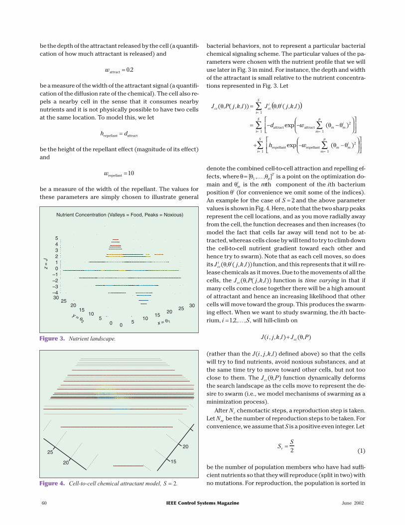
bacterial behaviors, not to represent a particular bacterialchemical signaling scheme. The particular values of the pa-rameters were chosen with the nutrient profile that we willuse later in Fig. 3 in mind. For instance, the depth and widthof the attractant is small relative to the nutrient concentra-tions represented in Fig. 3. Let

( )J P j k l J j k l

d

cci

S

cci i

i

S

( , ( , , )) , ( , , )θ θ θ=

= −

=

=

∑

∑1

1attract attract

repe

exp ( )− −

+

=

=

∑

∑

w

h

m

p

m mi

i

S

1

2

1

θ θ

llant repellantexp ( )− −

=∑wm

p

m mi

1

2θ θ

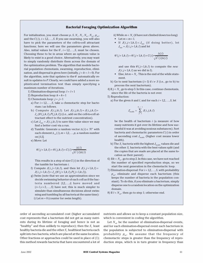
denote the combined cell-to-cell attraction and repelling ef-fects, where θ θ θ= [ , , ]1 K p

T is a point on the optimization do-main and θm

i is the mth component of the ith bacteriumposition θi (for convenience we omit some of the indices).An example for the case of S = 2 and the above parametervalues is shown in Fig. 4. Here, note that the two sharp peaksrepresent the cell locations, and as you move radially awayfrom the cell, the function decreases and then increases (tomodel the fact that cells far away will tend not to be at-tracted, whereas cells close by will tend to try to climb downthe cell-to-cell nutrient gradient toward each other andhence try to swarm). Note that as each cell moves, so doesits J j k lcc

i i( , ( , , ))θ θ function, and this represents that it will re-lease chemicals as it moves. Due to the movements of all thecells, the J P j k lcc( , ( , , ))θ function is time varying in that ifmany cells come close together there will be a high amountof attractant and hence an increasing likelihood that othercells will move toward the group. This produces the swarm-ing effect. When we want to study swarming, the ith bacte-rium, i S=1 2, , ,K , will hill-climb on

J i j k l J Pcc( , , , ) ( , )+ θ

(rather than the J i j k l( , , , ) defined above) so that the cellswill try to find nutrients, avoid noxious substances, and atthe same time try to move toward other cells, but not tooclose to them. The J Pcc( , )θ function dynamically deformsthe search landscape as the cells move to represent the de-sire to swarm (i.e., we model mechanisms of swarming as aminimization process).

After Nc chemotactic steps, a reproduction step is taken.Let Nre be the number of reproduction steps to be taken. Forconvenience, we assume that S is a positive even integer. Let

SS

r =2 (1)

be the number of population members who have had suffi-cient nutrients so that they will reproduce (split in two) withno mutations. For reproduction, the population is sorted in

60 IEEE Control Systems Magazine June 2002

543210

–1–2–3–4

zJ

=

3025

2015

105

0 05

1015

2025

30

Nutrient Concentration (Valleys = Food, Peaks = Noxious)

y = θ2 x = θ1

Figure 3. Nutrient landscape.

25

20 15

20

Figure 4. Cell-to-cell chemical attractant model, S = 2.

order of ascending accumulated cost (higher accumulatedcost represents that a bacterium did not get as many nutri-ents during its lifetime of foraging and hence is not as“healthy” and thus unlikely to reproduce); then the Sr leasthealthy bacteria die and the other Sr healthiest bacteria eachsplit into two bacteria, which are placed at the same location.Other fractions or approaches could be used in place of (1);this method rewards bacteria that have encountered a lot of

nutrients and allows us to keep a constant population size,which is convenient in coding the algorithm.

Let Ned be the number of elimination-dispersal events,and for each elimination-dispersal event each bacterium inthe population is subjected to elimination-dispersal withprobability ped . We assume that the frequency ofchemotactic steps is greater than the frequency of repro-duction steps, which is in turn greater in frequency than

June 2002 IEEE Control Systems Magazine 61

Bacterial Foraging Optimization Algorithm

For initialization, you must choose p, S, Nc , Ns , Nre , Ned , ped ,and the C i( ), i S= 12, , ,K . If you use swarming, you will alsohave to pick the parameters of the cell-to-cell attractantfunctions; here we will use the parameters given above.Also, initial values for the θi , i S= 12, , ,K , must be chosen.Choosing these to be in areas where an optimum value islikely to exist is a good choice. Alternatively, you may wantto simply randomly distribute them across the domain ofthe optimization problem. The algorithm that models bacte-rial population chemotaxis, swarming, reproduction, elimi-nation, and dispersal is given here (initially, j k l= = = 0). Forthe algorithm, note that updates to the θi automatically re-sult in updates to P. Clearly, we could have added a more so-phisticated termination test than simply specifying amaximum number of iterations.

1) Elimination-dispersal loop: l l= + 12) Reproduction loop: k k= + 13) Chemotaxis loop: j j= + 1

a) For i S= 12, , ,K , take a chemotactic step for bacte-rium i as follows.

b) Compute J i j k l( , , , ). Let J i j k l J i j k l( , , , ) ( , , , )= +J j k l P j k lcc

i( ( , , ), ( , , ))θ (i.e., add on the cell-to-cell at-tractant effect to the nutrient concentration).

c) Let J J i j k llast = ( , , , ) to save this value since we mayfind a better cost via a run.

d) Tumble: Generate a random vector ∆( )i p∈ � witheach element ∆ m i( ), m p= 12, , ,K , a random numberon [ , ]−11.

e) Move: Let

θ θi i

Tj k l j k l C i

i

i i( , , ) ( , , ) ( )

( )

( ) ( )+ = +1

∆∆ ∆

.

This results in a step of size C i( ) in the direction ofthe tumble for bacterium i.

f) Compute J i j k l( , , , )+ 1 , and then let J i j k l( , , , )+ =1J i j k l J j k l P j k lcc

i( , , , ) ( ( , , ), ( , , ))+ + + +1 1 1θ .g) Swim (note that we use an approximation since we

decide swimming behavior of each cell as if the bac-teria numbered { , , , }12 K i have moved and{ , , , }i i S+ +1 2 K have not; this is much simpler tosimulate than simultaneous decisions about swim-ming and tumbling by all bacteria at the same time):

i) Let m = 0 (counter for swim length).

ii) While m Ns< (if have not climbed down too long)• Let m m= + 1.• If J i j k l J( , , , )+ <1 last ( i f doing better), let

J J i j k llast = +( , , , )1 and let

θ θi i

Tj k l j k l C i

i

i i( , , ) ( , , ) ( )

( )

( ) ( )+ = + +1 1

∆∆ ∆

and use this θi j k l( , , )+ 1 to compute the newJ i j k l( , , , )+ 1 as we did in f).

• Else, letm Ns= . This is the end of the while state-ment.

h) Go to next bacterium (i + 1) if i S≠ (i.e., go to b) toprocess the next bacterium).

4) If j Nc< , go to step 3. In this case, continue chemotaxis,since the life of the bacteria is not over.

5) Reproduction:a) For the given k and l, and for each i S= 12, , ,K , let

J J i j k li

j

N c

health ==

+

∑1

1

( , , , )

be the health of bacterium i (a measure of howmany nutrients it got over its lifetime and how suc-cessful it was at avoiding noxious substances). Sortbacteria and chemotactic parameters C i( ) in orderof ascending cost Jhealth (higher cost means lowerhealth).

b) The Sr bacteria with the highest Jhealth values die andthe other Sr bacteria with the best values split (andthe copies that are made are placed at the same lo-cation as their parent).

6) Ifk Nre< , go to step 2. In this case, we have not reachedthe number of specified reproduction steps, so westart the next generation in the chemotactic loop.

7) Elimination-dispersal: For i S= 12, , ,K , with probabilityped , eliminate and disperse each bacterium (thiskeeps the number of bacteria in the population con-stant). To do this, if you eliminate a bacterium, simplydisperse one to a random location on the optimizationdomain.

8) If l Ned< , then go to step 1; otherwise end.

elimination-dispersal events (e.g., a bacterium will takemany chemotactic steps before reproduction, and severalgenerations may take place before an elimination-dis-persal event).

Clearly, we are ignoring many characteristics of the ac-tual biological optimization process in favor of simplicityand capturing the gross characteristics of chemotactichill-climbing and swarming. For instance, we ignore manycharacteristics of the chemical medium and we assumethat consumption does not affect the nutrient surface (e.g.,while a bacterium is in a nutrient-rich environment, we donot increase the value of J near where it has consumed nu-trients), where clearly in nature bacteria modify the nutri-ent concentrations via consumption. A tumble does notresult in a perfectly random new direction for movement;however, here we assume that it does. Brownian effectsbuffet the cell so that after moving a small distance, it iswithin a pie-shaped region with its start point at the tip ofthe piece of pie. Basically, we assume that swims arestraight, whereas in nature they are not. Tumble and runlengths are exponentially distributed random variables,not constant, as we assume. Run-length decisions are actu-ally based on the past 4 s of concentrations, whereas herewe assume that at each tumble, older information about nu-trient concentrations is lost. Although naturally asynchron-ous, we force synchronicity by requiring, for instance,chemotactic steps of different bacteria to occur at the sametime, all bacteria to reproduce at the same time instant, andall bacteria that are subjected to elimination and dispersalto do so at the same time. We assume a constant populationsize, even if there are many nutrients and generations. Weassume that the cells respond to nutrients in the environ-ment in the same way that they respond to ones released byother cells for the purpose of signaling the desire to swarm(a more biologically accurate model of the swarming behav-ior of certain bacteria is given in [22]). Clearly, otherchoices for the criterion of which bacteria should splitcould be used (e.g., based only on the concentration at theend of a cell’s lifetime, or on the quantity of noxious sub-stances that were encountered). We are also ignoring con-jugation and other evolutionary characteristics. Forinstance, we assume that C i( ), Ns , and Nc remain the samefor each generation. In nature it seems likely that these pa-rameters could evolve for different environments to maxi-mize population growth rates. The intent here was simply

to come up with a simple model that onlyrepresents certain aspects of the foragingbehavior of bacteria.

Guidelines forAlgorithm Parameter ChoicesThe bacterial foraging optimization algo-rithm requires specification of a variety ofparameters. First, you can pick the size of

the population, S. Clearly, increasing the size of S can signifi-cantly increase the computational complexity of the algo-rithm. However, for larger values of S, if you choose torandomly distribute the initial population, it is more likely thatyou will start at least some bacteria near an optimum point,and over time, it is then more likely that many bacterium willbe in that region, due to either chemotaxis or reproduction.

What should the values of the C i( ), i S=1 2, , ,K , be? Youcan choose a biologically motivated value; however, suchvalues may not be the best for an engineering application. IftheC i( )values are too large, then if the optimum value lies ina valley with steep edges, the search will tend to jump out ofthe valley, or it may simply miss possible local minima byswimming through them without stopping. On the otherhand, if the C i( ) values are too small, convergence can beslow, but if the search finds a local minimum it will typicallynot deviate too far from it. You should think of the C i( ) as atype of “step size” for the optimization algorithm.

The size of the values of the parameters that define thecell-to-cell attractant functions J cc

i will define the characteris-tics of swarming. If the attractant width is high and very deep,the cells will have a strong tendency to swarm (they mayeven avoid going after nutrients and favor swarming). On theother hand, if the attractant width is small and the depth shal-low, there will be little tendency to swarm and each cell willsearch on its own. Social versus independent foraging is thendictated by the balance between the strengths of thecell-to-cell attractant signals and nutrient concentrations.

Next, large values for Nc result in many chemotacticsteps, and hopefully more optimization progress, but ofcourse more computational complexity. If the size of Nc ischosen to be too short, the algorithm will generally relymore on luck and reproduction, and in some cases, it couldmore easily get trapped in a local minimum (premature con-vergence). You should think of Ns as creating a bias in therandom walk (which would not occur if Ns = 0), with largevalues tending to bias the walk more in the direction ofclimbing down the hill.

If Nc is large enough, the value of Nre affects how the algo-rithm ignores bad regions and focuses on good ones, sincebacteria in relatively nutrient-poor regions die (this models,with a fixed population size, the characteristic where bacte-ria will tend to reproduce at higher rates in favorable envi-ronments). If Nre is too small, the algorithm may convergeprematurely; however, larger values of Nre clearly increasecomputational complexity.

62 IEEE Control Systems Magazine June 2002

Our objective is to explain howmotile behaviors in both individualand groups of bacteria implementforaging and hence optimization.

A low value for Ned dictates that the algorithm will notrely on random elimination-dispersal events to try to find fa-vorable regions. A high value increases computational com-plexity but allows the bacteria to look in more regions tofind good nutrient concentrations. Clearly, if ped is large, thealgorithm can degrade to random exhaustive search. If,however, it is chosen appropriately, it can help the algo-rithm jump out of local optima and into a global optimum.

Connections with other NongradientGlobal Optimization MethodsThe reader already familiar with genetic algorithms (or evo-lutionary programming) may recognize the algorithmic anal-ogies between the fitness function and the nutrientconcentration function (both a type of landscape), selectionand bacterial reproduction (bacteria in the most favorableenvironments gain a selective advantage for reproduction),crossover and bacterial splitting (the children are at thesame concentration, whereas with crossover they generallyend up in a region around their parents on the fitness land-scape), and mutation and elimination and dispersal. How-ever, the algorithms are certainly not equivalent, andneither is a special case of the other. Each has its own distin-guishing features. The fitness function and nutrient concen-tration functions are not the same (one representslikelihood of survival for given phenotypic characteristics,whereas the other represents nutrient/noxious substanceconcentrations, or perhaps other environmental influencessuch as heat or light). Crossover represents mating and re-sulting differences in offspring, something we ignore in thebacterial foraging algorithm (we could, however, have madeless than perfect copies of the bacteria to represent theirsplitting). Moreover, mutation represents gene mutationand the resulting phenotypical changes, not physical dis-persal in a geographical area. From one perspective, notethat all the typical features of genetic algorithms could aug-ment the bacterial foraging algorithm by representing evo-lutionary characteristics of a forager in its environment.From another perspective, foraging algorithms can be inte-grated into evolutionary algorithms and thereby modelsome key survival activities that occur during the lifetime ofthe population that is evolving (i.e., foraging success canhelp define fitness, mating characteristics, etc.). For thebacteria studied here, foraging happens to entailhill-climbing via a type of biased random walk, and hencethe foraging algorithm can be viewed as a method to inte-grate a type of approximate stochastic gradient search(where only an approximation to the gradient is used, notanalytical gradient information) into evolutionary algo-rithms. Of course, standard gradient methods, quasi-New-ton methods, etc., depend on the use of an explicit analyticalrepresentation of the gradient, something that is not neededby a foraging or genetic algorithm. Lack of dependence onanalytical gradient information can be viewed as an advan-tage (fewer assumptions) or a disadvantage (e.g., since if

gradient information is available then the foraging or ge-netic algorithm may not exploit it properly).

There are in fact many approaches to “global optimiza-tion” when there is no explicit gradient information avail-able; however, it is beyond the scope of this article toevaluate the relative merits of foraging algorithms to thevast array of such methods that have been studied for manyyears. To start such a study, it makes sense to begin by con-sidering the theoretical convergence guarantees for certaintypes of evolutionary algorithms, stochastic approximationmethods, and pattern search methods (e.g., see [30] for

June 2002 IEEE Control Systems Magazine 63

30

25

20

15

10

5

0

30

25

20

15

10

5

0

30

25

20

15

10

5

0

30

25

20

15

10

5

0

0 0

00

10 10

1010

20 20

2020

30 30

3030

(a) (b)

(c) (d)

θ1 θ1

θ1θ1

θ 2θ 2

θ 2θ 2

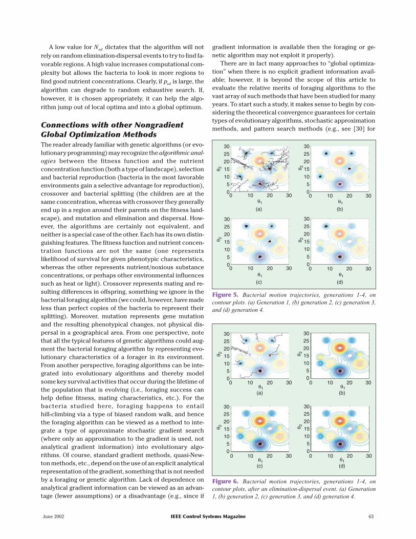
Figure 5. Bacterial motion trajectories, generations 1-4, oncontour plots. (a) Generation 1, (b) generation 2, (c) generation 3,and (d) generation 4.

302520151050

302520151050

302520151050

302520151050

θ 2θ 2

θ 2θ 2

θ1 θ1

θ1θ10 10 20 30 0 10 20 30

0 10 20 30 0 10 20 30

(a) (b)

(c) (d)

Figure 6. Bacterial motion trajectories, generations 1-4, oncontour plots, after an elimination-dispersal event. (a) Generation1, (b) generation 2, (c) generation 3, and (d) generation 4.

work along these lines) and then proceed to consider forag-ing algorithms in this context. Finally, note that evolutiondesigned the bacteria to forage in a time-varying and noisyenvironment (i.e., to achieve robust optimization for noisytime-varying cost functions). Can we exploit the character-istics of such an optimization approach for engineeringproblems?

Example: Function Optimization viaBacterial ForagingAs a simple illustrative example, we use the algorithm to tryto find the minimum of the function in Fig. 3 (note that thepoint [ , ]15 5 T is the global minimum point). To gain more in-sight into the operation of the algorithm, it is recommendedthat you run the algorithm yourself (see the sidebar on p. 61for a Web address from which you can obtain the code).

Nutrient Hill-Climbing: No SwarmingAccording to the above guidelines, choose S = 50, Nc =100,Ns = 4 (a biologically motivated choice), Nre = 4, Ned = 2,ped = 0 25. , and the C i( ) .= 01, i S=1 2, , ,K . The bacteria are ini-tially spread randomly over the optimization domain. Theresults of the simulation are illustrated by motion trajecto-ries of the bacteria on the contour plot of Fig. 3, as shown inFig. 5. In the first generation, starting from their random ini-tial positions, searching occurred in many parts of the opti-mization domain, and you can see the chemotactic motionsof the bacteria as the black trajectories where the peaks areavoided and the valleys are pursued. Reproduction picksthe 25 healthiest bacteria and copies them, and then asshown in Fig. 5 in generation 2, all the chemotactic steps arein five local minima. This again happens in going to genera-tions 3 and 4, but bacteria die in some of the local minima(due essentially to our requirement that the population size

stay constant), so that in generation 3 there are four groupsof bacteria in four local minima, whereas in generation 4there are two groups in two local minima.

Next, with the above choice of parameters there is an elim-ination-dispersal event, and we get the next four generationsshown in Fig. 6. Notice that elimination and dispersal shift thelocations of several of the bacteria, and thereby the algo-rithm explores other regions of the optimization domain.However, qualitatively we find a similar pattern to the previ-ous four generations where chemotaxis and reproductionwork together to find the global minimum; this time, how-ever, due to the large number of bacteria that were placednear the global minimum, after one reproduction step, all thebacteria are close to it (and remain this way). In this way, thebacterial population has found the global minimum.

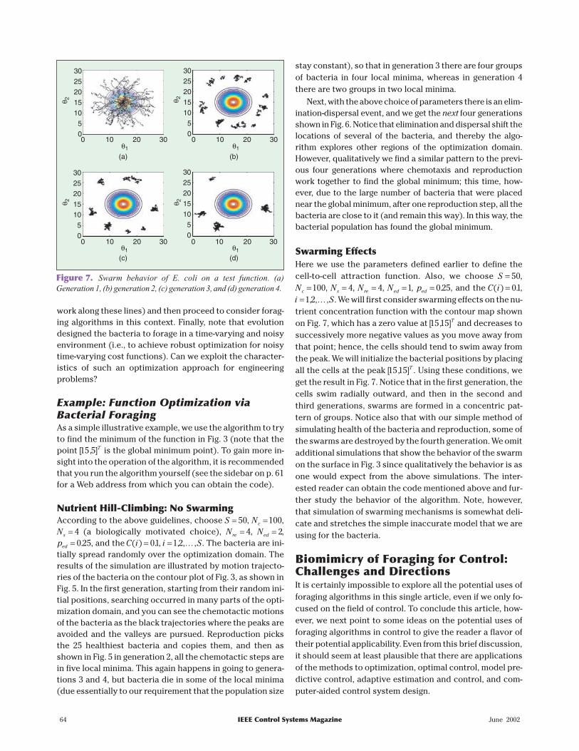
Swarming EffectsHere we use the parameters defined earlier to define thecell-to-cell attraction function. Also, we choose S = 50,Nc =100, Ns = 4, Nre = 4, Ned =1, ped = 0 25. , and the C i( ) .= 01,i S=1 2, , ,K . We will first consider swarming effects on the nu-trient concentration function with the contour map shownon Fig. 7, which has a zero value at [ , ]15 15 T and decreases tosuccessively more negative values as you move away fromthat point; hence, the cells should tend to swim away fromthe peak. We will initialize the bacterial positions by placingall the cells at the peak [ , ]15 15 T . Using these conditions, weget the result in Fig. 7. Notice that in the first generation, thecells swim radially outward, and then in the second andthird generations, swarms are formed in a concentric pat-tern of groups. Notice also that with our simple method ofsimulating health of the bacteria and reproduction, some ofthe swarms are destroyed by the fourth generation. We omitadditional simulations that show the behavior of the swarmon the surface in Fig. 3 since qualitatively the behavior is asone would expect from the above simulations. The inter-ested reader can obtain the code mentioned above and fur-ther study the behavior of the algorithm. Note, however,that simulation of swarming mechanisms is somewhat deli-cate and stretches the simple inaccurate model that we areusing for the bacteria.

Biomimicry of Foraging for Control:Challenges and DirectionsIt is certainly impossible to explore all the potential uses offoraging algorithms in this single article, even if we only fo-cused on the field of control. To conclude this article, how-ever, we next point to some ideas on the potential uses offoraging algorithms in control to give the reader a flavor oftheir potential applicability. Even from this brief discussion,it should seem at least plausible that there are applicationsof the methods to optimization, optimal control, model pre-dictive control, adaptive estimation and control, and com-puter-aided control system design.

64 IEEE Control Systems Magazine June 2002

30

25

20

15

10

5

0

30

25

20

15

10

5

0

30

25

20

15

10

5

0

30

25

20

15

10

5

00 10 20 30 0 10 20 30

0 10 20 30 0 10 20 30

θ1

θ 2θ 2 θ 2

θ 2

θ1θ1

θ1

(a) (b)

(c) (d)

Figure 7. Swarm behavior of E. coli on a test function. (a)Generation 1, (b) generation 2, (c) generation 3, and (d) generation 4.

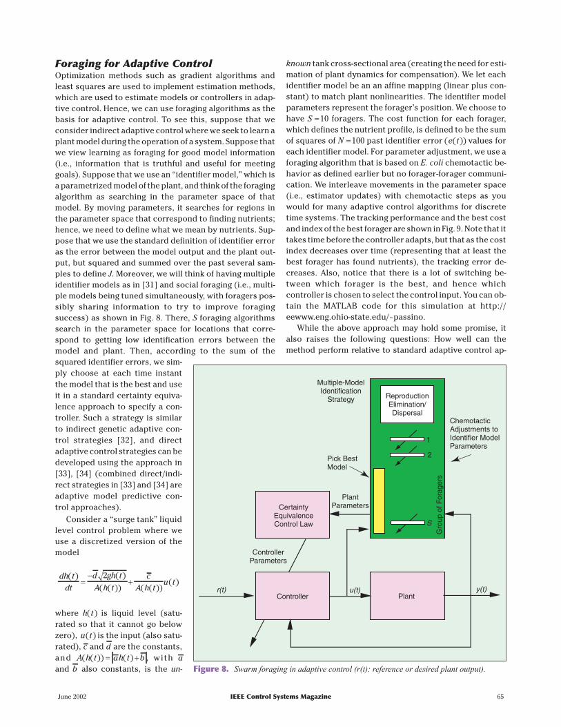
Foraging for Adaptive ControlOptimization methods such as gradient algorithms andleast squares are used to implement estimation methods,which are used to estimate models or controllers in adap-tive control. Hence, we can use foraging algorithms as thebasis for adaptive control. To see this, suppose that weconsider indirect adaptive control where we seek to learn aplant model during the operation of a system. Suppose thatwe view learning as foraging for good model information(i.e., information that is truthful and useful for meetinggoals). Suppose that we use an “identifier model,” which isa parametrized model of the plant, and think of the foragingalgorithm as searching in the parameter space of thatmodel. By moving parameters, it searches for regions inthe parameter space that correspond to finding nutrients;hence, we need to define what we mean by nutrients. Sup-pose that we use the standard definition of identifier erroras the error between the model output and the plant out-put, but squared and summed over the past several sam-ples to define J. Moreover, we will think of having multipleidentifier models as in [31] and social foraging (i.e., multi-ple models being tuned simultaneously, with foragers pos-sibly sharing information to try to improve foragingsuccess) as shown in Fig. 8. There, S foraging algorithmssearch in the parameter space for locations that corre-spond to getting low identification errors between themodel and plant. Then, according to the sum of thesquared identifier errors, we sim-ply choose at each time instantthe model that is the best and useit in a standard certainty equiva-lence approach to specify a con-troller. Such a strategy is similarto indirect genetic adaptive con-trol strategies [32], and directadaptive control strategies can bedeveloped using the approach in[33], [34] (combined direct/indi-rect strategies in [33] and [34] areadaptive model predictive con-trol approaches).

Consider a “surge tank” liquidlevel control problem where weuse a discretized version of themodel

dh tdt

d gh t

A h tc

A h tu t

( ) ( )

( ( )) ( ( ))( )=

−+

2

where h t( ) is liquid level (satu-rated so that it cannot go belowzero), u t( ) is the input (also satu-rated), c and d are the constants,and A h t ah t b( ( )) ( )= + , with aand b also constants, is the un-

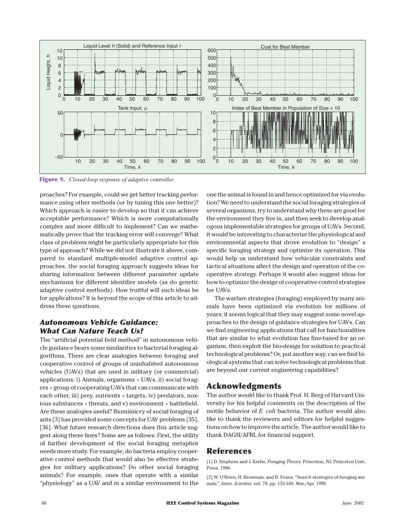
known tank cross-sectional area (creating the need for esti-mation of plant dynamics for compensation). We let eachidentifier model be an an affine mapping (linear plus con-stant) to match plant nonlinearities. The identifier modelparameters represent the forager’s position. We choose tohave S =10 foragers. The cost function for each forager,which defines the nutrient profile, is defined to be the sumof squares of N =100 past identifier error ( ( ))e t values foreach identifier model. For parameter adjustment, we use aforaging algorithm that is based on E. coli chemotactic be-havior as defined earlier but no forager-forager communi-cation. We interleave movements in the parameter space(i.e., estimator updates) with chemotactic steps as youwould for many adaptive control algorithms for discretetime systems. The tracking performance and the best costand index of the best forager are shown in Fig. 9. Note that ittakes time before the controller adapts, but that as the costindex decreases over time (representing that at least thebest forager has found nutrients), the tracking error de-creases. Also, notice that there is a lot of switching be-tween which forager is the best, and hence whichcontroller is chosen to select the control input. You can ob-tain the MATLAB code for this simulation at http://eewww.eng.ohio-state.edu/~passino.

While the above approach may hold some promise, italso raises the following questions: How well can themethod perform relative to standard adaptive control ap-

June 2002 IEEE Control Systems Magazine 65

CertaintyEquivalenceControl Law

Controller Plant

ReproductionElimination/Dispersal

Gro

up o

f For

ager

s1

2

S

ChemotacticAdjustments toIdentifier ModelParameters

Multiple-ModelIdentification

Strategy

ControllerParameters

r(t) u(t) y(t)

Pick BestModel

PlantParameters

Figure 8. Swarm foraging in adaptive control (r(t): reference or desired plant output).

proaches? For example, could we get better tracking perfor-mance using other methods (or by tuning this one better)?Which approach is easier to develop so that it can achieveacceptable performance? Which is more computationallycomplex and more difficult to implement? Can we mathe-matically prove that the tracking error will converge? Whatclass of problems might be particularly appropriate for thistype of approach? While we did not illustrate it above, com-pared to standard multiple-model adaptive control ap-proaches, the social foraging approach suggests ideas forsharing information between different parameter updatemechanisms for different identifier models (as do geneticadaptive control methods). How fruitful will such ideas befor applications? It is beyond the scope of this article to ad-dress these questions.

Autonomous Vehicle Guidance:What Can Nature Teach Us?The “artificial potential field method” in autonomous vehi-cle guidance bears some similarities to bacterial foraging al-gorithms. There are clear analogies between foraging andcooperative control of groups of uninhabited autonomousvehicles (UAVs) that are used in military (or commercial)applications: i) Animals, organisms = UAVs, ii) social forag-ers = group of cooperating UAVs that can communicate witheach other, iii) prey, nutrients = targets, iv) predators, nox-ious substances = threats, and v) environment = battlefield.Are these analogies useful? Biomimicry of social foraging ofants [3] has provided some concepts for UAV problems [35],[36]. What future research directions does this article sug-gest along these lines? Some are as follows: First, the utilityof further development of the social foraging metaphorneeds more study. For example, do bacteria employ cooper-ative control methods that would also be effective strate-gies for military applications? Do other social foraginganimals? For example, ones that operate with a similar“physiology” as a UAV and in a similar environment to the

one the animal is found in and hence optimized for via evolu-tion? We need to understand the social foraging strategies ofseveral organisms, try to understand why these are good forthe environment they live in, and then seek to develop anal-ogous implementable strategies for groups of UAVs. Second,it would be interesting to characterize the physiological andenvironmental aspects that drove evolution to “design” aspecific foraging strategy and optimize its operation. Thiswould help us understand how vehicular constraints andtactical situations affect the design and operation of the co-operative strategy. Perhaps it would also suggest ideas forhow to optimize the design of cooperative control strategiesfor UAVs.

The warfare strategies (foraging) employed by many ani-mals have been optimized via evolution for millions ofyears; it seems logical that they may suggest some novel ap-proaches to the design of guidance strategies for UAVs. Canwe find engineering applications that call for functionalitiesthat are similar to what evolution has fine-tuned for an or-ganism, then exploit the bio-design for solution to practicaltechnological problems? Or, put another way, can we find bi-ological systems that can solve technological problems thatare beyond our current engineering capabilities?

The author would like to thank Prof. H. Berg of Harvard Uni-versity for his helpful comments on the description of themotile behavior of E. coli bacteria. The author would alsolike to thank the reviewers and editors for helpful sugges-tions on how to improve the article. The author would like tothank DAGSI/AFRL for financial support.

References[1] D. Stephens and J. Krebs, Foraging Theory. Princeton, NJ: Princeton Univ.Press, 1986.

[2] W. O’Brien, H. Browman, and B. Evans, “Search strategies of foraging ani-mals,” Amer. Scientist, vol. 78, pp. 152-160, Mar./Apr. 1990.

66 IEEE Control Systems Magazine June 2002

12

10

8

6

4

2

0

Liqu

id H

eigh

t,h

50

0

–50

10 10

1010

20 20

2020

30 30

3030

40 40

4040

50 50

5050

60 60

6060

70 70

7070

80 80

8080

90 90

9090

100 100

100100

Liquid Level (Solid) and Reference Inputh r

Tank Input, u

Time, k

0 0

0

600

500

400

300

200

100

0

Cost for Best Member

10

8

6

4

2

0

Index of Best Member in Population of Size = 10

Time, k

Figure 9. Closed-loop response of adaptive controller.

[3] E. Bonabeau, M. Dorigo, and G. Theraulaz, Swarm Intelligence: From Natu-ral to Artificial Systems. New York: Oxford Univ. Press, 1999.

[4] C. Adami, Introduction to Artificial Life. New York: Springer-Verlag, 1998.

[5] M. Resnick, Turtles, Termites, and Traffic Jams: Explorations in MassivelyParallel Microworlds. Cambridge, MA: MIT Press, 1994.

[6] S. Levy, Artificial Life: A Report from the Frontier where Computers Meet Biol-ogy. New York: Vintage Books, 1992.

[7] T. Audesirk and G. Audesirk, Biology: Life on Earth, 5th ed. EnglewoodCliffs, NJ: Prentice Hall, 1999.

[8] H. Berg, “Motile behavior of bacteria,” Phys. Today, pp. 24-29, Jan. 2000.

[9] M. Madigan, J. Martinko, and J. Parker, Biology of Microorganisms, 8th ed.Englewood Cliffs, NJ: Prentice Hall, 1997.

[10] F. Neidhardt, J. Ingraham, and M. Schaechter, Physiology of the BacterialCell: A Molecular Approach. Sunderland, MA: Sinauer, 1990.

[11] B. Alberts, D. Bray, J. Lewis, M. Raff, K. Roberts, and J. Watson, MolecularBiology of the Cell, 2nd ed. New York: Garland Publishing, 1989.

[12] H. Berg and D. Brown, “Chemotaxis in escherichia coli analysed bythree-dimensional tracking,” Nature, vol. 239, pp. 500-504, Oct. 1972.

[13] J. Segall, S. Block, and H. Berg, “Temporal comparisons in bacterialchemotaxis,” Proc. Nat. Acad. Sci., vol. 83, pp. 8987-8991, Dec. 1986.

[14] H. Berg, Random Walks in Biology. Princeton, NJ: Princeton Univ. Press,1993.

[15] D. DeRosier, “The turn of the screw: The bacterial flagellar motor,” Cell,vol. 93, pp. 17-20, 1998.

[16] G. Lowe, M. Meister, and H. Berg, “Rapid rotation of flagellar bundles inswimming bacteria,” Nature, vol. 325, pp. 637-640, Oct. 1987.

[17] T.-M. Yi, Y. Huang, M. Simon, and J. Doyle, “Robust perfect adaptation inbacterial chemotaxis through integral feedback control,” PNAS, vol. 97, pp.4649-4653, April 25, 2000.

[18] J. Armitage, “Bacterial tactic responses,” Adv. Microbial Phys., vol. 41, pp.229-290, 1999.

[19] E. Budrene and H. Berg, “Dynamics of formation of symmetrical patternsby chemotactic bacteria,” Nature, vol. 376, pp. 49-53, 1995.

[20] Y. Blat and M. Eisenbach, “Tar-dependent and -independent pattern for-mation by salmonella typhimurium,” J. Bacteriology, vol. 177, pp. 1683-1691,Apr. 1995.

[21] E. Budrene and H. Berg, “Complex patterns formed by motile cells ofescherichia coli,” Nature, vol. 349, pp. 630-633, Feb. 1991.

[22] D. Woodward, R. Tyson, M. Myerscough, J. Murray, E. Budrene, and H.Berg, “Spatio-temporal patterns generated by salmonella typhimurium,”Biophysi. J., vol. 68, pp. 2181-2189, 1995.

[23] R. Losick and D. Kaiser, “Why and how bacteria communicate,” Sci.Amer., vol. 276, no. 2, pp. 68-73, 1997.

[24] M. McBride, P. Hartzell, and D. Zusman, “Motility and tactic behavior ofmyxococcus xanthus,” in Myxobacteria II, M. Dworkin and D. Kaiser, Eds.Washington, DC: American Society for Microbiology, 1993, pp. 285-305.

[25] L. Shimkets and M. Dworkin, “Myxobacterial multicellularity,” in Bacteriaas Multicellular Organisms, J. Shapiro and M. Dworkin, Eds., New York: OxfordUniv. Press, 1997, pp. 220-244.

[26] H. Reichenbach, “Biology of the myxobacteria: Ecology and taxonomy,”in Myxobacteria II, M. Dworkin and D. Kaiser, Eds. Washington, DC: AmericanSociety for Microbiology, 1993, pp. 13-62.

[27] J. Shapiro, “Bacteria as multicellular organisms,” Sci. Amer., vol. 258, pp.62-69, 1988.

[28] A. Stevens, “Simulations of the gliding behavior and aggregation ofmyxobacteria,” in Biological Motion (Lecture Notes in Biomathematics, vol.89), W. Alt and G. Hoffmann, Eds. Berlin: Springer-Verlag, 1990, pp. 548-555.

[29] A. Stevens, “A stochastic cellular automaton, modeling gliding and aggre-gation of myxobacteria,” SIAM J. Appli. Math., vol. 61, no. 1, pp. 172-182, 2000.

[30] J. Spall, S. Hill, and D. Stark, “Some theoretical comparisons of stochasticoptimization approaches,” in Proc. American Control Conf., Chicago, IL, June2000, pp. 1904-1908.

[31] R. Murray-Smith and T.A. Johansen, Eds., Multiple Model Approaches toNonlinear Modeling and Control. London, UK: Taylor and Francis, 1996.

[32] K. Kristinsson and G. Dumont, “System identification and control usinggenetic algorithms,” IEEE Trans. Syst., Man, Cybernet., vol. 22, no. 5, pp.1033-1046, 1992.

[33] L.L. Porter and K. Passino, “Genetic adaptive and supervisory control,”Int. J. Intell. Contr. Syst., vol. 12, no. 1, pp. 1-41, 1998.

[34] W. Lennon and K. Passino, “Genetic adaptive identification and control,”Eng. Applicat. Artif. Intell., vol. 12, pp. 185-200, Apr. 1999.

[35] S. Brueckner and H. Parunak, “Multiple pheromones for improved guid-ance,” in Proceedings AEC, 2000 [Online]. Available: www.erim.org/cec/pro-jects/adaptiv/

[36] M. Krieger, J.-B. Billeter, and L. Keller, “Ant-like task allocation and re-cruitment in cooperative robots,” Nature, vol. 406, pp. 992-995, Aug. 2000.

Kevin M. Passino received his Ph.D. in electrical engineer-ing from the University of Notre Dame in 1989. He hasworked on control systems research at Magnavox Elec-tronic Systems Co. and McDonnell Aircraft Co. He is cur-rently a Professor in the Department of ElectricalEngineering at The Ohio State University and Director of theCollaborative Center of Control Science that is supportedby AFRL/VA and AFOSR. He was the Program Chair of the2001 IEEE Conference on Decision and Control. He hasserved as the Vice President of Technical Activities of theIEEE Control Systems Society (CSS); was an elected memberof the IEEE Control Systems Society Board of Governors;was Chair for the IEEE CSS Technical Committee on Intelli-gent Control; has been an Associate Editor for IEEE Transac-tions on Automatic Control and IEEE Transactions on FuzzySystems; has served as a Guest Editor for IEEE Control Sys-tems Magazine and IEEE Expert Magazine; and was on the Ed-itorial Board of the International Journal for EngineeringApplications of Artificial Intelligence. He was the ProgramChair for the 8th IEEE International Symposium on Intelli-gent Control, 1993, and the General Chair for the 11th IEEEInternational Symposium on Intelligent Control. He iscoeditor or coauthor of five books. He is a Senior Member ofthe IEEE.

June 2002 IEEE Control Systems Magazine 67