Embed Size (px)
DESCRIPTION
file ini merupakan file yang berisi informasi mengenai apa itu modulasi
Citation preview
Baseband Modulation and Demodulation
Digital CommunicationElektro Diponegoro
Wahyul Amien [email protected]
3
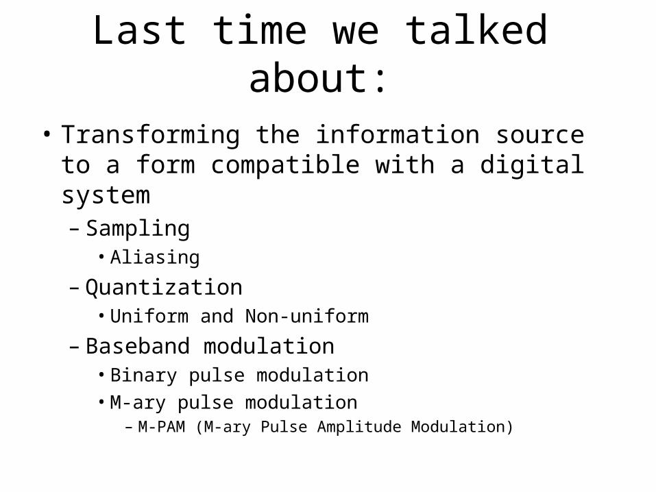
Last time we talked about:
• Transforming the information source to a form compatible with a digital system– Sampling
• Aliasing
– Quantization• Uniform and Non-uniform
– Baseband modulation• Binary pulse modulation
• M-ary pulse modulation– M-PAM (M-ary Pulse Amplitude Modulation)

Formatting and Transmission of Baseband Signal
– Information (data) rate:– Symbol rate :
• For real time transmission:
Sampling at rate
(sampling time=Ts)
Quantizing each sampled value to one of the L levels in quantizer.
Encoding each q. value to bits
(Data bit duration Tb=Ts/l)
Encode
PulsemodulateSample Quantize
Pulse waveforms(baseband signals)
Bit stream(Data bits)
Format
Digital info.
Textual info.
Analog info.
source
Mapping every data bits to a symbol out of M symbols and transmitting
a baseband waveform with duration T
ss Tf /1 Ll 2log
Mm 2log
[bits/sec] /1 bb TR ec][symbols/s /1 TR
mRRb
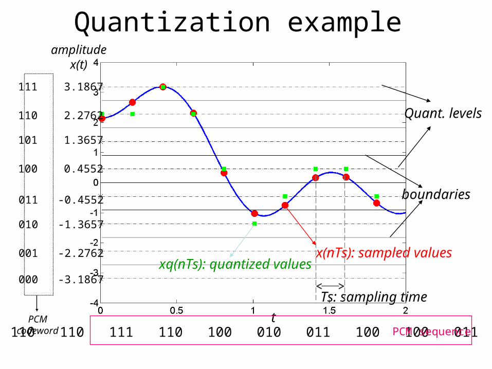
Quantization example
t
Ts: sampling time
x(nTs): sampled valuesxq(nTs): quantized values
boundaries
Quant. levels
111 3.1867
110 2.2762
101 1.3657
100 0.4552
011 -0.4552
010 -1.3657
001 -2.2762
000 -3.1867
PCMcodeword 110 110 111 110 100 010 011 100 100 011 PCM sequence
amplitudex(t)
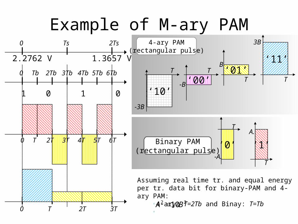
Example of M-ary PAM
0 Tb 2Tb 3Tb 4Tb 5Tb 6Tb
0 Ts 2Ts
0 T 2T 3T
2.2762 V 1.3657 V
1 1 0 1 0 1-B
B
T‘01’
3B
TT
-3B
T
‘00’‘10’
‘1’
A.
T
‘0’
T
-A.
Assuming real time tr. and equal energy per tr. data bit for binary-PAM and 4-ary PAM:
•4-ary: T=2Tb and Binay: T=Tb•
4-ary PAM(rectangular pulse)
Binary PAM(rectangular pulse)
‘11’
0 T 2T 3T 4T 5T 6T
22 10BA

Today we are going to talk about:
• Receiver structure– Demodulation (and sampling)– Detection
• First step for designing the receiver– Matched filter receiver
• Correlator receiver
• Vector representation of signals (signal space), an important tool to facilitate – Signals presentations, receiver structures– Detection operations

Demodulation and Detection
• Major sources of errors:– Thermal noise (AWGN)
• disturbs the signal in an additive fashion (Additive)• has flat spectral density for all frequencies of interest (White)• is modeled by Gaussian random process (Gaussian Noise)
– Inter-Symbol Interference (ISI)• Due to the filtering effect of transmitter, channel and receiver,
symbols are “smeared”.
FormatPulse
modulateBandpassmodulate
Format DetectDemod.
& sample
)(tsi)(tgiim
im̂ )(tr)(Tz
channel)(thc
)(tn
transmitted symbol
estimated symbol
Mi ,,1 M-ary modulation
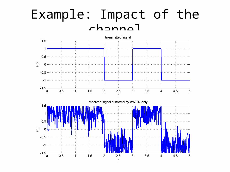
Example: Impact of the channel
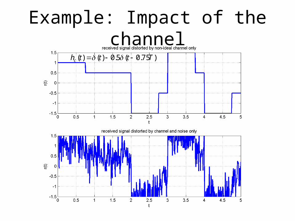
)75.0(5.0)()( Tttthc
Example: Impact of the channel

Receiver’s Job
• Demodulation and Sampling: – Waveform recovery and preparing the received
signal for detection:• Improving the signal power to the noise power
(SNR) using matched filter
• Reducing ISI using equalizer
• Sampling the recovered waveform
• Detection:– Estimate the transmitted symbol based on the
received sample

Receiver Structure
Frequencydown-conversion
Receiving filter
Equalizingfilter
Threshold comparison
For bandpass signals Compensation for channel induced ISI
Baseband pulse(possibly distored)
Sample (test statistic)
Baseband pulseReceived waveform
Step 1 – waveform to sample transformation Step 2 – decision making
)(tr)(Tz
im̂
Demodulate & Sample Detect
Baseband and Bandpass
• Bandpass model of detection process is equivalent to baseband model because:– The received bandpass waveform is first
transformed to a baseband waveform.– Equivalence theorem:
• Performing bandpass linear signal processing followed by heterodying the signal to the baseband, yields the same results as heterodying the bandpass signal to the baseband , followed by a baseband linear signal processing.
Steps in Receiver Design
• Find optimum solution for receiver design with the following goals: 1. Maximize SNR2. Minimize ISI
• Steps in design:– Model the received signal– Find separate solutions for each of the goals.
• First, we focus on designing a receiver which maximizes the SNR.

Design the Receiver Filter to Maximize the SNR
• Model the received signal
• Simplify the model:– Received signal in AWGN
)(thc)(tsi
)(tn
)(tr
)(tn
)(tr)(tsiIdeal channels
)()( tthc
AWGN
AWGN
)()()()( tnthtstr ci
)()()( tntstr i
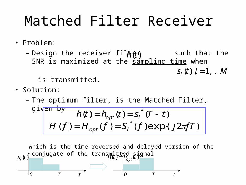
Matched Filter Receiver • Problem:
– Design the receiver filter such that the SNR is maximized at the sampling time when
is transmitted.• Solution:
– The optimum filter, is the Matched Filter, given by
which is the time-reversed and delayed version of the conjugate of the transmitted signal
)(th
)()()( * tTsthth iopt )2exp()()()( * fTjfSfHfH iopt
Mitsi ,...,1 ),(
T0 t
)(tsi
T0 t
)()( thth opt

Example of Matched Filter
T t T t T t0 2T
)()()( thtsty opti 2A)(tsi )(thopt
T t T t T t0 2T
)()()( thtsty opti 2A)(tsi )(thopt
T/2 3T/2T/2 TT/2
2
2TA
TA
TA
TA
TA
TA
TA
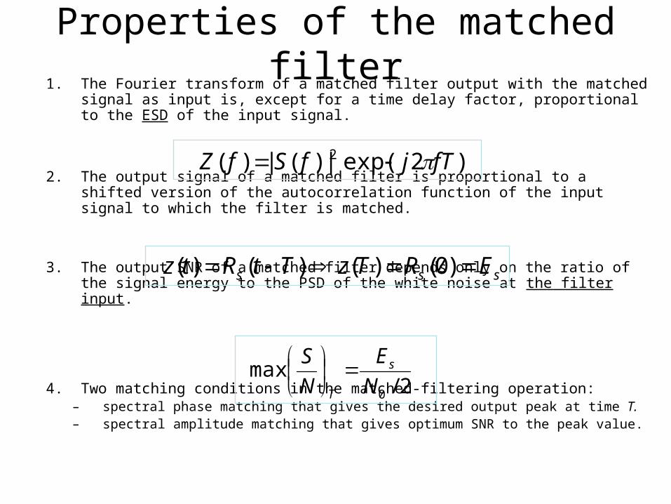
Properties of the matched filter1. The Fourier transform of a matched filter output with the matched signal
as input is, except for a time delay factor, proportional to the ESD of the input signal.
2. The output signal of a matched filter is proportional to a shifted version of the autocorrelation function of the input signal to which the filter is matched.
3. The output SNR of a matched filter depends only on the ratio of the signal energy to the PSD of the white noise at the filter input.
4. Two matching conditions in the matched-filtering operation:– spectral phase matching that gives the desired output peak at time T.– spectral amplitude matching that gives optimum SNR to the peak value.
)2exp(|)(|)( 2 fTjfSfZ
sss ERTzTtRtz )0()()()(
2/max
0N
E
N
S s
T
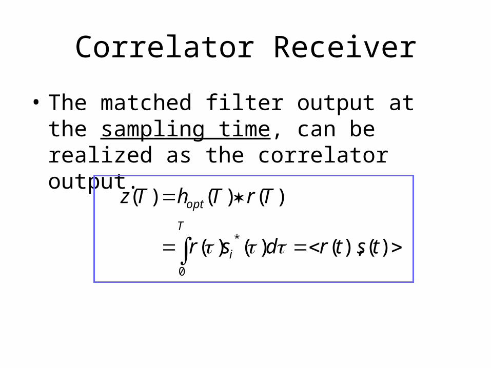
Correlator Receiver
• The matched filter output at the sampling time, can be realized as the correlator output.
)(),()()(
)()()(
*
0
tstrdsr
TrThTz
i
T
opt

Implementation of Matched Filter Receiver
)()( tTstrz ii Mi ,...,1
),...,,())(),...,(),(( 2121 MM zzzTzTzTz z
Mz
z
1
z)(tr
)(1 Tz)(*
1 tTs
)(* tTsM )(TzM
z
Bank of M matched filters
Matched filter output:Observation
vector
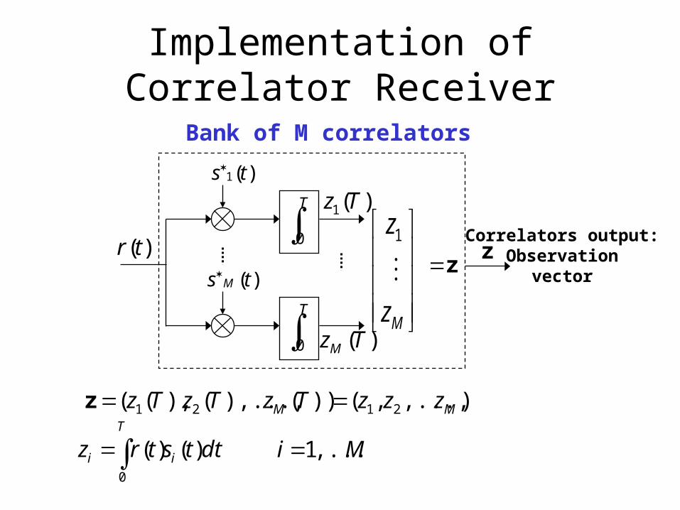
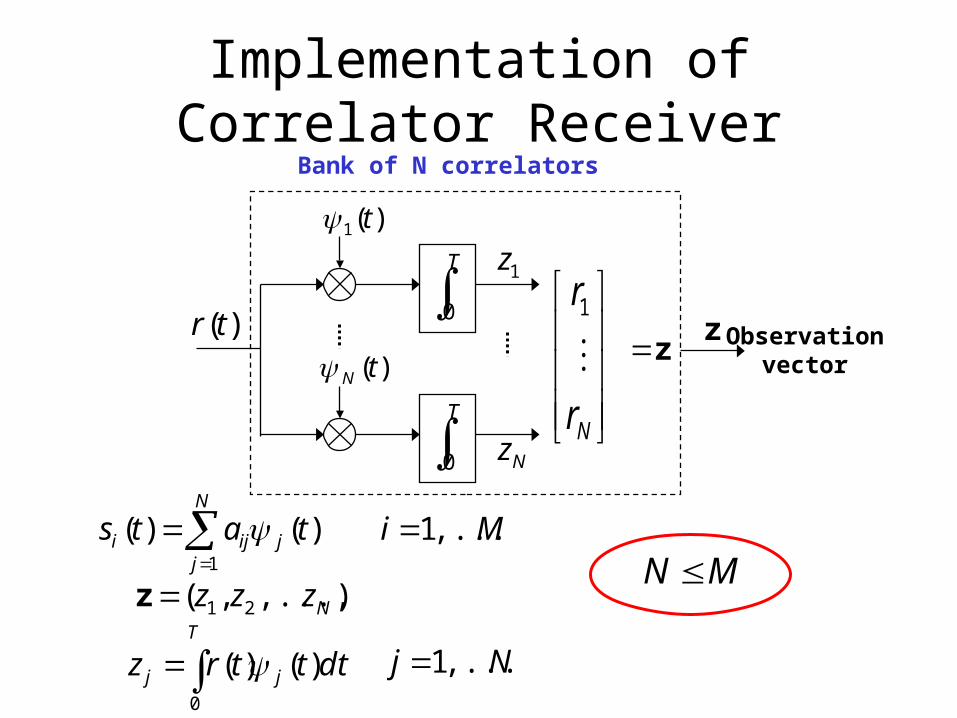
Implementation of Correlator Receiver
dttstrz i
T
i )()(0
T
0
)(1 ts
T
0
)(ts M
Mz
z
1
z)(tr
)(1 Tz
)(TzM
z
Bank of M correlators
Correlators output:Observation
vector
),...,,())(),...,(),(( 2121 MM zzzTzTzTz z
Mi ,...,1
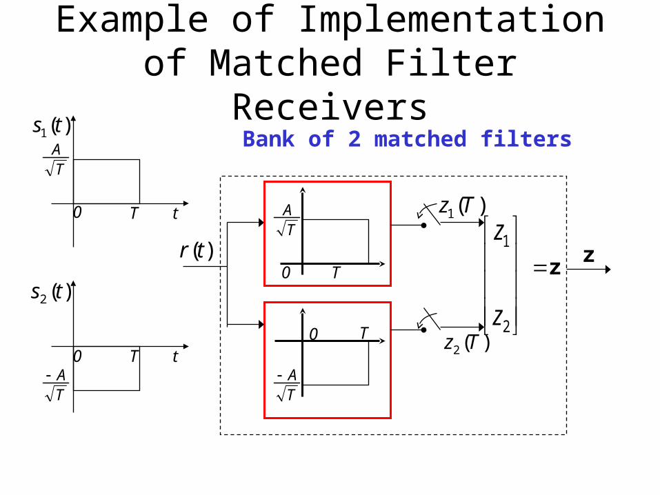
Example of Implementation of Matched Filter Receivers
2
1
z
zz
)(tr
)(1 Tz
)(2 Tz
z
Bank of 2 matched filters
T t
)(1 ts
T t
)(2 tsT
T0
0
TA
TA
TA
TA
0
0
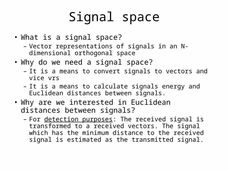
Signal space
• What is a signal space?– Vector representations of signals in an N-dimensional
orthogonal space
• Why do we need a signal space?– It is a means to convert signals to vectors and vice vrs– It is a means to calculate signals energy and Euclidean
distances between signals.
• Why are we interested in Euclidean distances between signals?– For detection purposes: The received signal is transformed
to a received vectors. The signal which has the minimum distance to the received signal is estimated as the transmitted signal.
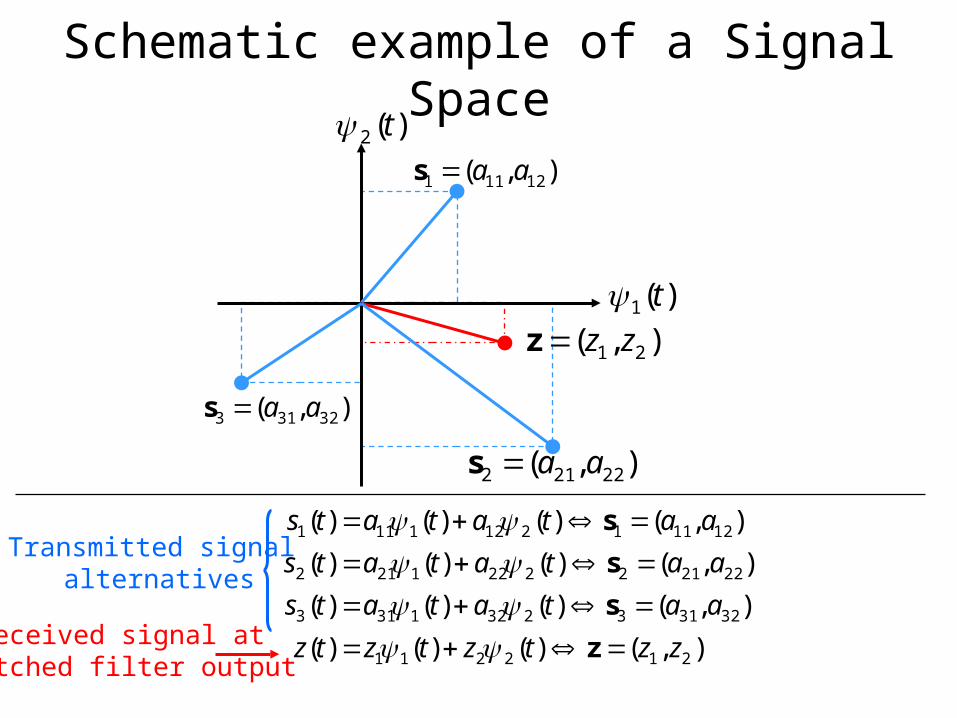
Schematic example of a Signal Space
),()()()(
),()()()(
),()()()(
),()()()(
212211
323132321313
222122221212
121112121111
zztztztz
aatatats
aatatats
aatatats
z
s
s
s
)(1 t
)(2 t),( 12111 aas
),( 22212 aas
),( 32313 aas
),( 21 zzz
Transmitted signal alternatives
Received signal at matched filter output
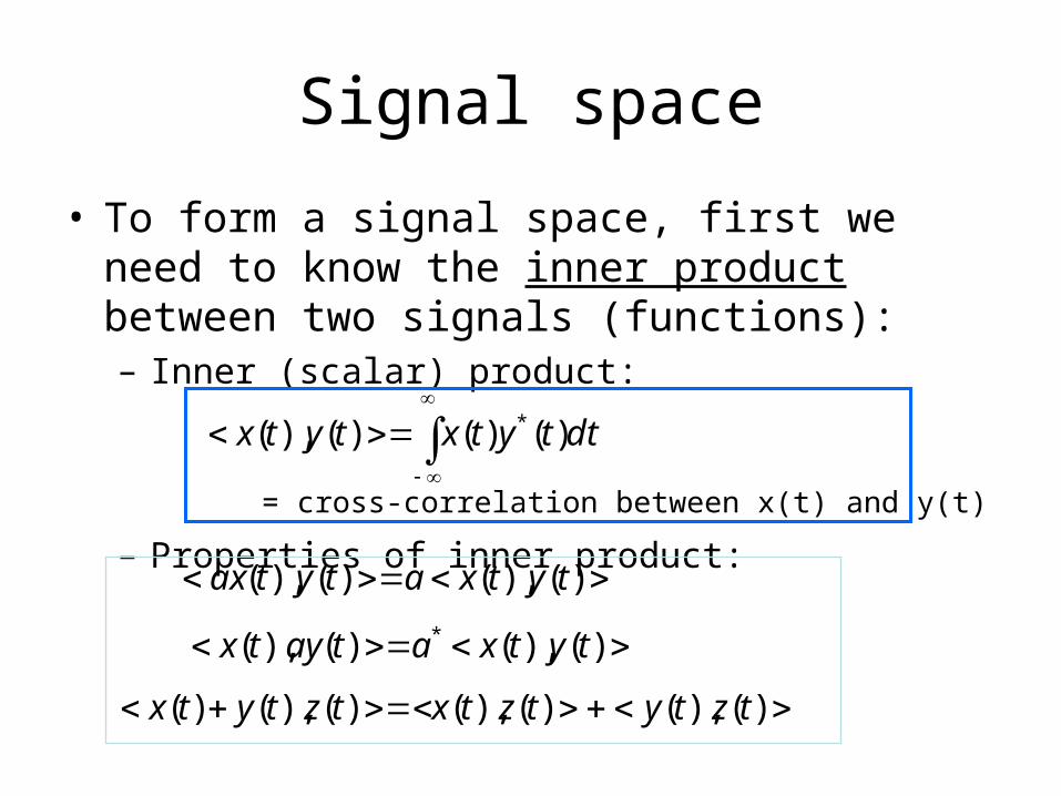
Signal space
• To form a signal space, first we need to know the inner product between two signals (functions):– Inner (scalar) product:
– Properties of inner product: )(),()(),( tytxatytax
)(),()(),( * tytxataytx
)(),()(),()(),()( tztytztxtztytx
dttytxtytx )()()(),( *
= cross-correlation between x(t) and y(t)
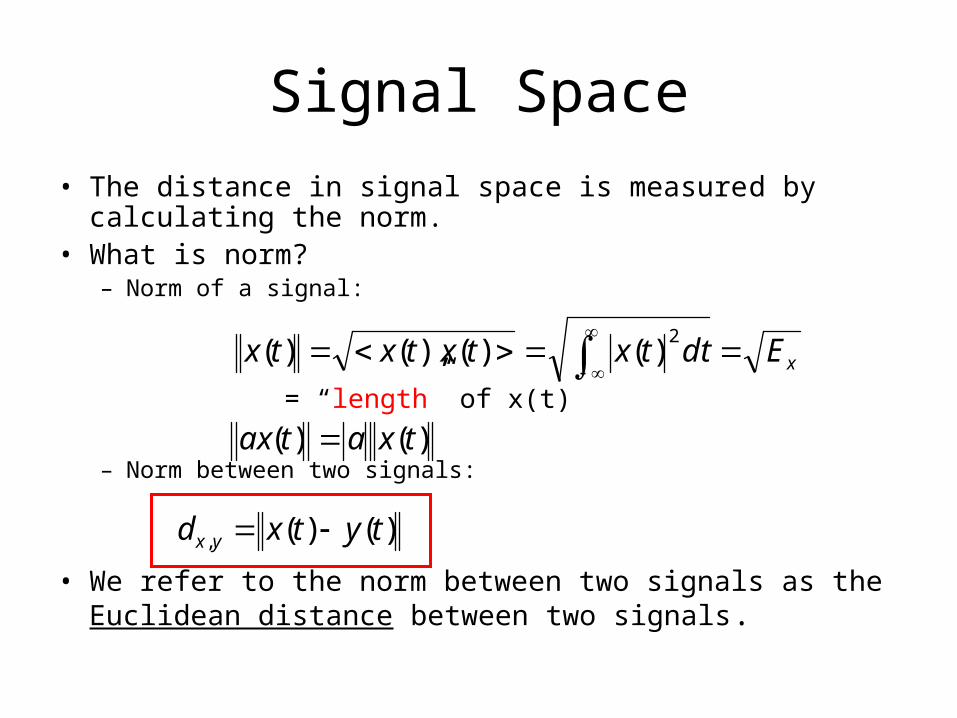
Signal Space
• The distance in signal space is measured by calculating the norm.
• What is norm?– Norm of a signal:
– Norm between two signals:
• We refer to the norm between two signals as the Euclidean distance between two signals.
)()(, tytxd yx
xEdttxtxtxtx
2)()(),()(
)()( txatax = “length” of x(t)
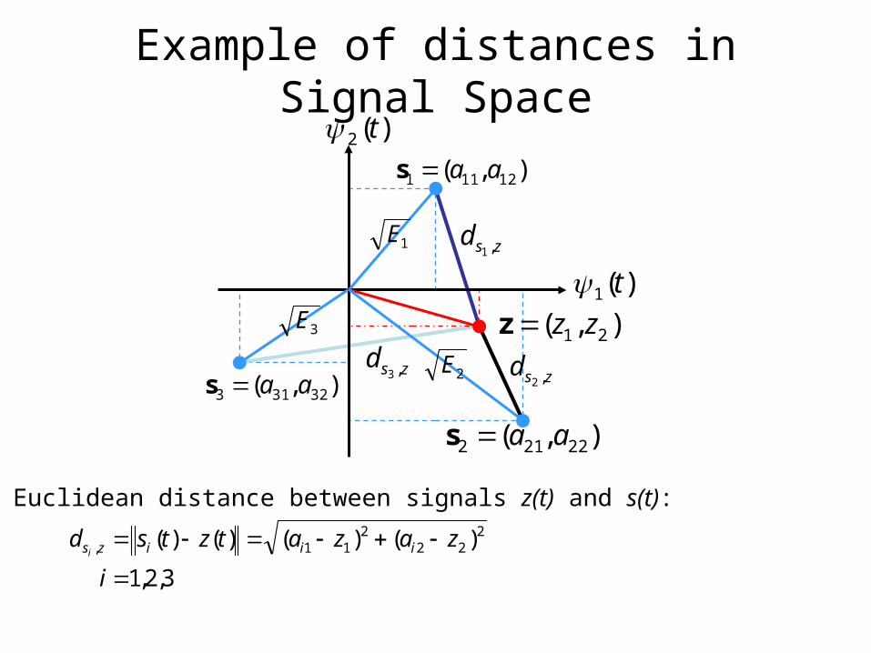
Example of distances in Signal Space
)(1 t
)(2 t),( 12111 aas
),( 22212 aas
),( 32313 aas
),( 21 zzz
zsd ,1
zsd ,2zsd ,3
The Euclidean distance between signals z(t) and s(t):
3,2,1
)()()()( 222
211,
i
zazatztsd iiizsi
1E
3E
2E
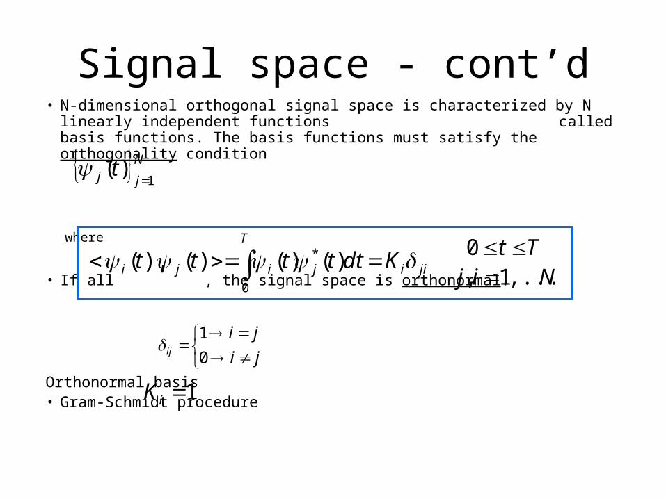
Signal space - cont’d• N-dimensional orthogonal signal space is characterized by N linearly
independent functions called basis functions. The basis functions must satisfy the orthogonality condition
where
• If all , the signal space is orthonormal.
Orthonormal basis• Gram-Schmidt procedure
N
jj t1
)(
jiij
T
iji Kdttttt )()()(),( *
0
Tt 0Nij ,...,1,
ji
jiij 0
1
1iK
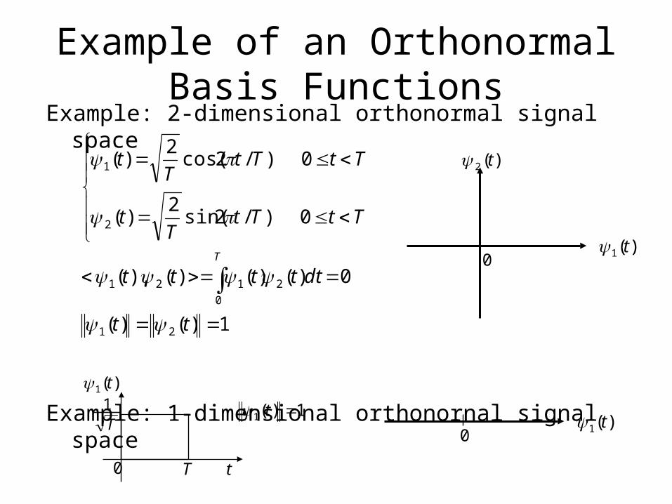
Example of an Orthonormal Basis Functions
Example: 2-dimensional orthonormal signal space
Example: 1-dimensional orthonornal signal space
1)()(
0)()()(),(
0)/2sin(2
)(
0)/2cos(2
)(
21
2
0
121
2
1
tt
dttttt
TtTtT
t
TtTtT
t
T
)(1 t
)(2 t
0
T t
)(1 t
T1
0
1)(1 t)(1 t
0
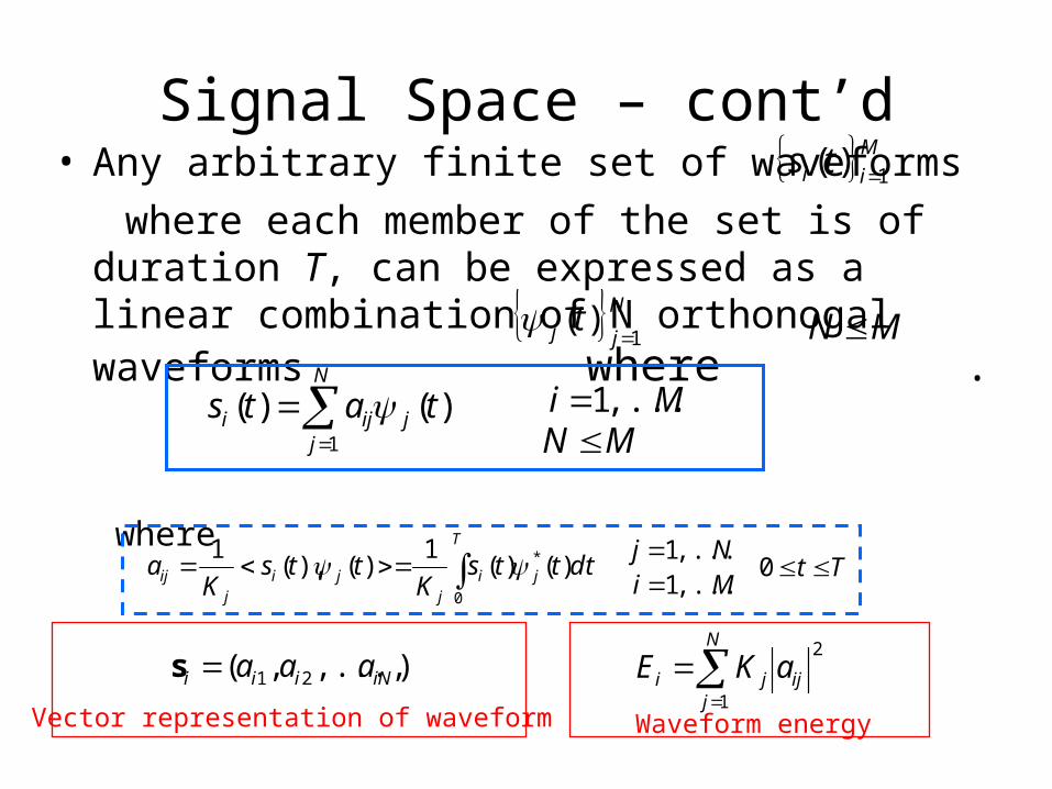
Signal Space – cont’d• Any arbitrary finite set of waveforms
where each member of the set is of duration T, can be expressed as a linear combination of N orthonogal waveforms where .
where
M
ii ts 1)(
N
jj t1
)(
MN
N
jjiji tats
1
)()( Mi ,...,1MN
dtttsK
ttsK
aT
jij
jij
ij )()(1
)(),(1
0
* Tt 0Mi ,...,1Nj ,...,1
),...,,( 21 iNiii aaas2
1ij
N
jji aKE
Vector representation of waveform Waveform energy

Signal Space - cont’d
N
jjiji tats
1
)()( ),...,,( 21 iNiii aaas
iN
i
a
a
1
)(1 t
)(tN
1ia
iNa
)(tsi
T
0
)(1 t
T
0
)(tN
iN
i
a
a
1
ms)(tsi
1ia
iNa
ms
Waveform to vector conversion Vector to waveform conversion

Example of Projecting Signals to an Orthonormal Signal Space
),()()()(
),()()()(
),()()()(
323132321313
222122221212
121112121111
aatatats
aatatats
aatatats
s
s
s
)(1 t
)(2 t ),( 12111 aas
),( 22212 aas
),( 32313 aas
Transmitted signal alternatives
dtttsaT
jiij )()(0 Tt 0Mi ,...,1Nj ,...,1
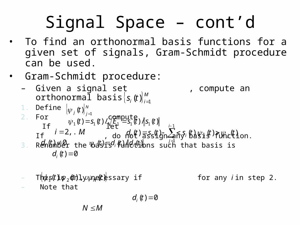
Signal Space – cont’d• To find an orthonormal basis functions for a given set
of signals, Gram-Schmidt procedure can be used.• Gram-Schmidt procedure:
– Given a signal set , compute an orthonormal basis1. Define2. For compute If let
If , do not assign any basis function.3. Renumber the basis functions such that basis is
– This is only necessary if for any i in step 2. – Note that
M
ii ts 1)(
N
jj t1
)(
)(/)(/)()( 11111 tstsEtst
Mi ,...,2
1
1
)()(),()()(i
jjjiii tttststd
0)( tdi )(/)()( tdtdt iii 0)( tdi
)(),...,(),( 21 ttt N
0)( tdi
MN
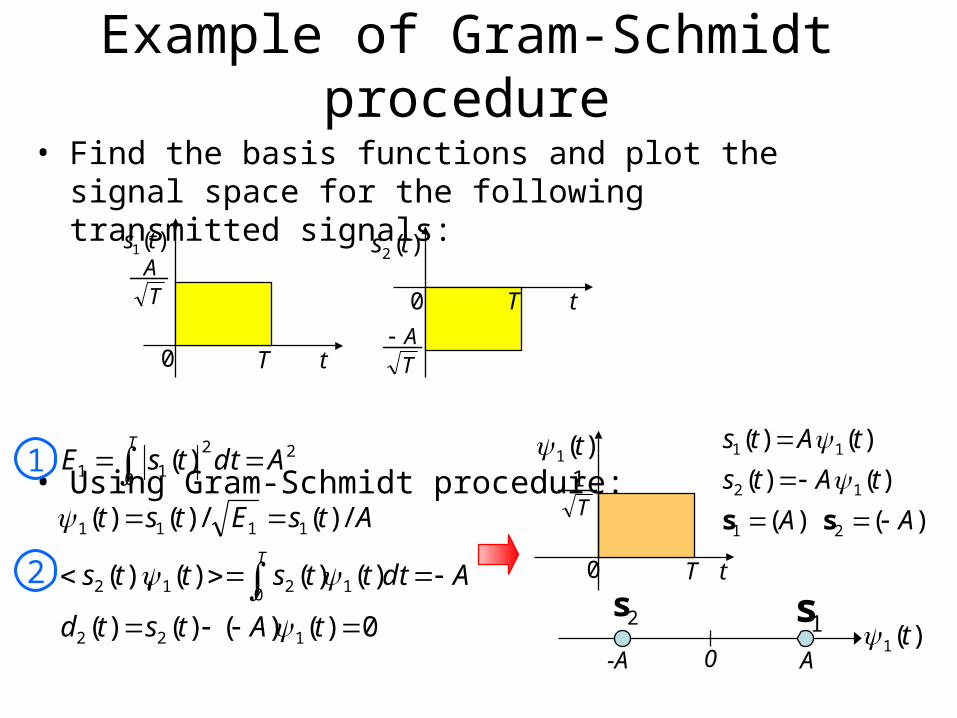
Example of Gram-Schmidt procedure
• Find the basis functions and plot the signal space for the following transmitted signals:
• Using Gram-Schmidt procedure:
)( )(
)()(
)()(
21
12
11
AA
tAts
tAts
ss
)(1 t-A A0
1s2s
T t
)(1 ts
T t
)(2 ts
TA
TA
0
0
T t
)(1 t
T1
0
0)()()()(
)()()(),(
/)(/)()(
)(
122
0 1212
1111
0
22
11
tAtstd
Adtttstts
AtsEtst
AdttsE
T
T
1
2
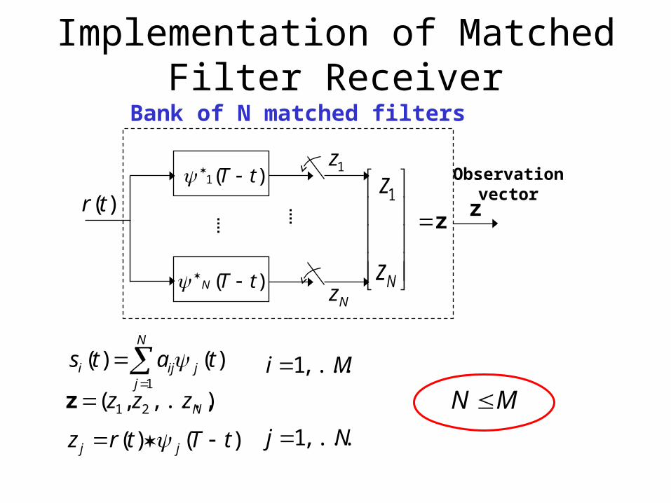
Implementation of Matched Filter Receiver
)(tr
1z)(1 tT
)( tTN Nz
Bank of N matched filters
Observationvector
)()( tTtrz jj Nj ,...,1
),...,,( 21 Nzzzz
N
jjiji tats
1
)()(
MN Mi ,...,1
Nz
z1
z z
Implementation of Correlator Receiver
dtttrz j
T
j )()(0
),...,,( 21 Nzzzz
Nj ,...,1
T
0
)(1 t
T
0
)(tN
Nr
r
1
z)(tr
1z
Nz
z
Bank of N correlators
Observationvector
N
jjiji tats
1
)()( Mi ,...,1MN
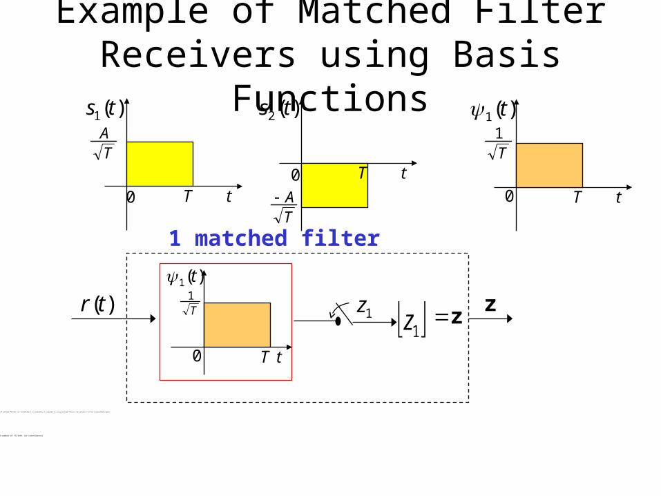
Example of Matched Filter Receivers using Basis Functions
– Number of matched filters (or correlators) is reduced by 1 compared to using matched filters (correlators) to the transmitted signal.
• Reduced number of filters (or correlators)
1z z)(tr z
1 matched filter
T t
)(1 t
T1
0
1z
T t
)(1 ts
T t
)(2 ts
T t
)(1 t
T1
0
TA
TA0
0
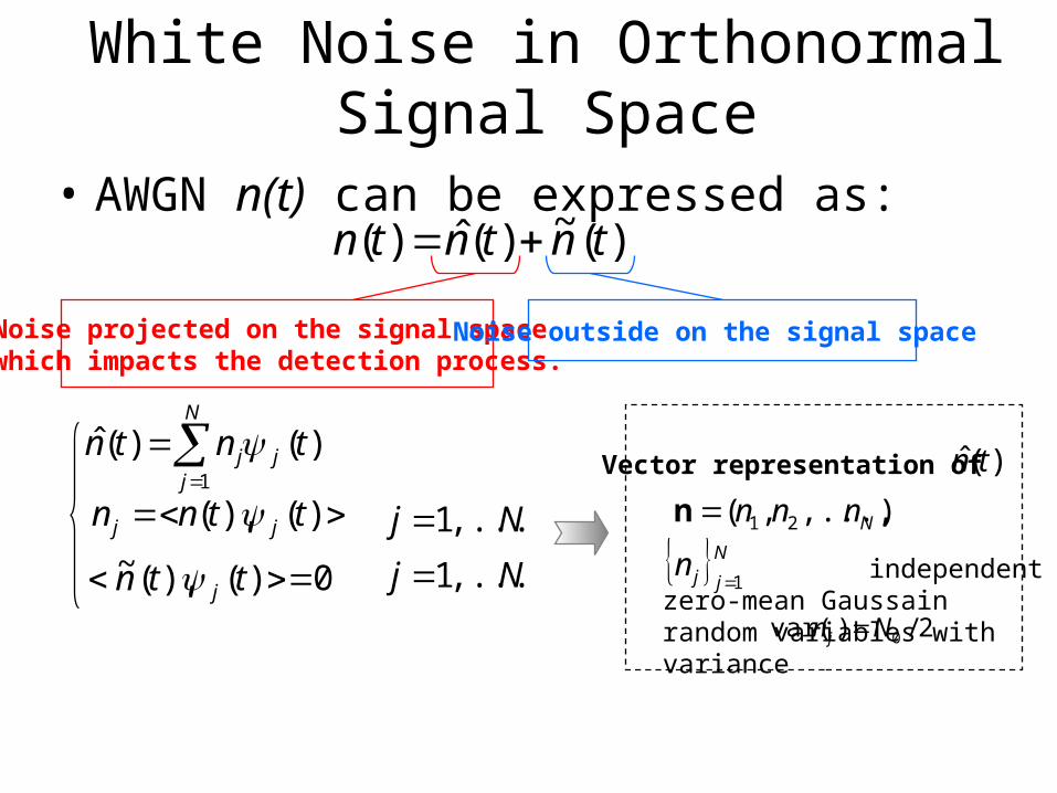
White Noise in Orthonormal Signal Space
• AWGN n(t) can be expressed as:)(~)(ˆ)( tntntn
Noise projected on the signal space which impacts the detection process.
Noise outside on the signal space
)(),( ttnn jj
0)(),(~ ttn j
)()(ˆ1
tntnN
jjj
Nj ,...,1
Nj ,...,1
Vector representation of
),...,,( 21 Nnnnn
)(ˆ tn
independent zero-mean Gaussain random variables with variance
N
jjn1
2/)var( 0Nn j