Embed Size (px)
Citation preview
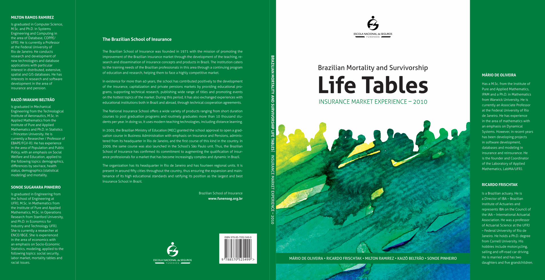
Mário de oliveira • ricardo FriSchtak • Milton raMirez • kaizô Beltrão • Sonoe Pinheiro
Mário de oLiveira
Has a m.sc. from the Institute of
pure and applied mathematics,
Ipam and a ph.D. in mathematics
from Warwick university. He is
currently an associate professor
at the Federal university of rio
de Janeiro. He has experience
in the area of mathematics with
an emphasis on Dynamical
systems. However, in recent years
has been developing projects
in software development,
databases and modeling in
insurance and reinsurance. He
is the founder and coordinator
of the Laboratory of applied
mathematics, Labma/uFrJ.
ricardo FrischTak
Is a Brazilian actuary. He is
a Director of IBa – Brazilian
Institute of actuaries and
represents IBa on the council of
the Iaa – International actuarial
association. He was a professor
of actuarial science at the uFrJ
– Federal university of rio de
Janeiro. He holds a ph.D. degree
from cornell university. His
hobbies include motorcycling,
sailing and off-road car driving.
He is married and has two
daughters and five grandchildren.
kaizô iwakaMi BeLTrão
Is graduated in mechanical engineering from the technological Institute of aeronautics, m.sc. in applied mathematics from the Institute of pure and applied mathematics and ph.D. in statistics – princeton university. He is currently a researcher / professor of EBAPE/FGV-RJ. He has experience in the area of population and public policy, with an emphasis on social Welfare and education, applied to the following topics: demographics, differences by sex/race, health status, demographics (statistical modeling) and mortality.
MiLTon raMos raMirez
Is graduated in computer science, m.sc. and ph.D. in systems engineering and computing in the area of Database, cOppe/uFrJ. He is currently a professor at the Federal university of rio de Janeiro. He conducts research and development of new technologies and database applications with particular interest in distributed, extensive, spatial and GIs databases. He has interests in research and software development in the area of insurance and pension.
sonoe sugahara Pinheiro
Is graduated in engineering from the school of engineering at uFrJ, m.sc. in mathematics from the Institute of pure and applied mathematics, m.sc. in Operations research from stanford university, and ph.D. in economics for Industry and technology uFrJ. she is currently a researcher at ence/IBGe. she is experienced in the area of economics with an emphasis on Socio-Economic statistics, modeling, applied to the following topics: social security, labor market, mortality tables and racial issues.
Bra
ziLian
Mo
rTaLiTY
an
d su
rviv
or
shiP LiFe Ta
BLes in
SUra
nc
e Ma
rket eXPerien
ce – 2010
CONFERIR E, CASO NECESSÁRIO, AJUSTAR LOMBADA
Brazilian Mortality and Survivorship
Life TablesInsurance market experIence – 2010
9 788570 525499
ISBN 978-85-7052-549-9
The Brazilian school of insurance
the Brazilian school of Insurance was founded in 1971 with the mission of promoting the
improvement of the Brazilian insurance market through the development of the teaching, re-
search and dissemination of insurance concepts and products in Brazil. the institution caters
to the training needs of the Brazilian professionals in this area through a continuing program
of education and research, helping them to face a highly competitive market.
In existence for more than 40 years, the school has contributed positively to the development
of the insurance, capitalization and private pensions markets by providing educational pro-
grams, supporting technical research, publishing wide range of titles and promoting events
on the hottest topics of the market. During this period, it has also exchanged experiences with
educational institutions both in Brazil and abroad, through technical cooperation agreements.
The National Insurance School offers a wide variety of products ranging from short duration
courses to post graduation programs and routinely graduates more than 10 thousand stu-
dents per year. In doing so, it uses modern teaching technologies, including distance learning.
In 2005, the Brazilian ministry of education (mec) granted the school approval to open a grad-
uation course in Business administration with emphasis on Insurance and pensions, adminis-
tered from its headquarter in Rio de Janeiro, and the first course of this kind in the country. In
2009, the same course was also launched in the school’s são paulo unit. thus, the Brazilian
School of Insurance has confirmed its commitment to augmenting the qualification of insur-
ance professionals for a market that has become increasingly complex and dynamic in Brazil.
the organization has its headquarter in rio de Janeiro and has fourteen regional units. It is
present in around fifty cities throughout the country, thus ensuring the expansion and main-
tenance of its high educational standards and ratifying its position as the largest and best
Insurance school in Brazil.
Brazilian school of Insurance
www.funenseg.org.br

Brazilian Mortality and Survivorship
Life TablesInsurance market experIence – 2010

Brazilian Mortality and Survivorship
Life TablesInsurance market experIence – 2010
Mário de oliveira
ricardo FriSchtak
Milton raMirez
kaizô Beltrão
Sonoe Pinheiro
rio de Janeiro – 2012
Brazilian Mortality and Survivorship
Life TablesInsurance market experIence – 2010
Mário de oliveira
ricardo FriSchtak
Milton raMirez
kaizô Beltrão
Sonoe Pinheiro
rio de Janeiro – 2012

1st Edition: December 2012Fundação Escola Nacional de Seguros – FunensegRua Senador Dantas, 74 – Térreo, 2º, 3º, 4º e 14º andaresRio de Janeiro – RJ – Brazil – CEP 20031-205Phone: (21) 3380-1000Fax: (21) 3380-1546Internet: www.funenseg.org.brE-mail: [email protected]
Printed in Brazil
No part of this book may be reproduced or transmitted in any form or any manner: electronic, mechanical, photographic, recorded, or by any other means without permission in writing from the Fundação Escola Nacional de Seguros – Funenseg.
Editorial CoordinationDirectorate of Higher Education and Research/Publications Coordination
EditingVera de SouzaMariana Santiago
Graphic ProductionHercules Rabello
Front Cover/LayoutGrifo Design
Reviewer Monica Teixeira Dantas Savini
Virginia Thomé – CRB-7/3242Librarian responsible for preparation of the catalogue card
B839 Brazilian mortality and survivorship life tables : insurance market experience 2010 / Mário de Oliveira ... /et al/. -- Rio Janeiro : Funenseg, 2012. 100 p. ; 26 cm
ISBN nº 978-85-7052-549-9. Authors who participated in the preparation of the book: Ricardo Frischtak, Milton Ramirez, Kaizô Beltrão e Sonoê Pinheiro.
1. Mortality Table – Brasil. 2. Biometric Table – Mortality – Brazil. 3. Mortality – Table – Brasil. 4. Actuarial – Biometric Table - Brasil. I. Oliveira, Mário de. II. Title.
0012-1144 CDU 368.01
Acknowledgments
W e thank all the members of the FenaPrevi Actuarial Committee who contributed with their suggestions and discussion in all phases of our work. Our special thanks go to Jair Lacerda, Francisco Pereira, Luiz Pelegrino and Beatriz Herranz
who accompanied the project of constructing these tables from its inception.
We appreciate the collaboration of the Ministry of Social Security and Dataprev for the pro-vision of supplementary information contributing to the success of this project.
This research project was achieved with the support of FAPERJ –, Foundation for Support and Research for the State of Rio de Janeiro, within the “PRIORITY RIO” programme and the Support Program for Education and Research Institutions in the State of Rio de Janeiro.
We thank our students at LabMA/UFRJ, in particular Paulo Vitor, for revising the graphic content of this book.

Contents
1. Presentation ...................................................................................................................... 9
1. introduction ................................................................................................................... 11
2. Brief history of Mortality tables ................................................................................ 13
3. Mortality graduation ..................................................................................................... 17
3.1 Introduction ........................................................................................................... 17
3.2 Distributions .......................................................................................................... 19
3.3 Criteria for model choice ....................................................................................... 20
4. database construction ................................................................................................. 21
4.1 The insured population .......................................................................................... 21
4.2 The “Tábuas” database .......................................................................................... 23
5. Selection of subpopulations ...................................................................................... 27
5.1 Population distribution and evolution in time ....................................................... 27
5.2 IBNR estimates ..................................................................................................... 32
5.3 Consideration on extreme age groups ................................................................... 33
5.4 Selection criteria for exclusion of subpopulations ................................................ 33
5.5 Differentiation of mortality curves according to sex and coverage ...................... 39
6. construction of life and Survival tables ................................................................. 45
6.1 Heligman & Pollard model ................................................................................... 45
6.2 Methodology for the parameters estimation .......................................................... 52
6.3 Curvefitting ........................................................................................................... 53
7 Br-ems tables ................................................................................................................. 67
7.1 Male survivorship: Br-Emssb-V.2010-M .............................................................. 68
7.2 Male mortality: Br-Emsmt-V.2010-M ................................................................... 72
7.3 Female survivorship: Br-Emssb-V.2010-F ............................................................ 76
7.4 Female mortality: Br-Emsmt-V.2010-F ................................................................. 80
7.5 Comparison of Br-Ems with well-known tables ................................................... 84
7.6 Examples of the use of Br-Ems Tables .................................................................. 90
references ............................................................................................................................ 93

9
Presentation
t his book presents the survival and mortality biometric tables as the product of a commissioned research by Fenaprevi – Federação Nacional de Previdência Privada e Vida [National Federation of Private Pension and Life] to the Laboratory of Applied
Mathematics at the Mathematical Institute of the Federal University of Rio de Janeiro.
TheresearchrepresentsamilestonesinceBrazilianstatisticsarebeingappliedforthefirsttime, which means that pension funds and insurance institutions now have at their disposal amorereliablerepresentationoftheBrazilianpopulation’sprofile.Morethan300millionrecords from 23 insurance companies were used with detailed information on insurance con-tracts, broken down by gender, age and type of plan. These data were also crossed-referenced with the statistics from the register of the Death Control System at the National Registry of Information. No less important, were the team of researchers: some exceptional individuals who have international recognition, which provides credibility to the new biometric tables.
With these new tables, named BR-EMS, Brazilian institutions – insurance companies, pen-sion companies, regulatory and supervisory agencies, universities, research centres and con-sultingfirms–willhaveaccesstoafundamentaltoolforgreateroperationalefficiencyandsolvency of the system.
The Brazilian College of Insurance, as an educational and research institution, is proud to publish and disseminate this research, thereby reinforcing its partnership agreement with the LabMA/UFRJ – Laboratory of Applied Mathematics at the Mathematical Institute of the Federal University of Rio de Janeiro.
Professor Claudio Contador, Ph.D. Brazilian College of Insurance


11
1 Introduction
d uring the first decade of the current century, theBrazilian life insurancemarketexpanded at an accelerated rate. Insurance companies operating in Brazil were using foreign life tables, since there were no local life tables available.
Consequently, FenaPrevi – the National Federation of Open Pension Funds and Life Insurance Companies – commissioned LabMA/UFRJ – the Applied Mathematics Lab of the Mathematics Institute of the Federal University of Rio de Janeiro – to construct life tables for the Brazilian insurance market.
This project was followed by SUSEP – the Brazilian Supervising Insurance Authority.
The present work describes the methodology used and presents the survival and mortali-ty tables constructed thereof, based on the experience of the Brazilian insurance life prod-ucts market, for the years 2004, 2005 and 2006. Data was provided by a pool of Insurance Companies, representing an 82% share of the market.
These life tables were named Experiência do Mercado Segurador Brasileiro, BR-EMS (Experience of the Brazilian Insurance Market) and consist of four variants for mortality (male and female) and survivorship (male and female). The variants were given the following names: BR-EMSsb-v.2010-m, BR-EMSsb-v.2010-f, BR-EMSmt-v.2010-m e BR-EMSmt-v.2010-f, where “sb” denotes survivorship, “mt” mortality, “m” male and “f” female.
SUSEP established tables BR-EMS as Standard Life Tables for the Brazilian Insurance Market. SUSEP also demanded that they be reviewed in 2015.
We would like to thank all members of the Actuarial Committee of FenaPrevi who contributed with suggestions and discussions in all phases of the project. We also thank our students of LabMA/UFRJ, especially Paulo Vitor who was responsible for redrafting all the graphs in this book. This research was partially supported by FAPERJ.


13
2 Brief history of Mortality Tables
l ife tables have existed for a long time in human history. There is evidence that in ancient Rome, in the 3rd century B.C., the State collected and elaborated statistics for life and death, probably using life table schemes, calculating life expectancy at birth
andotherages(Duchene&Wunsch,1988).However, thefirstscientificreferencestolifetables occur in the work of John Graunt, “Natural and political observations made upon the bills of mortality”, published in 1662 (apud David, 1998), and notably the seminal paper by astronomer Edmond Halley, in 1693 (apud Duchene & Wunsch, 1988) where the basis of actuarial science were laid.
Since then, numerous tables have been compiled for different countries and regions, as well as ta-blesforspecificpurposestosupporttheactuarialworkofinsurancecompaniesandpensionfunds.
Life tables are an important tool to help with the establishment of public policies, such as health, education, economic planning, workforce allocation, social security, insurance in gen-eral, and investment planning.
Therearetwoissueswhenoneconsidersconstructingalifetableforaspecificpopulationgroup:
i) Thefirst concerns the data itself,mostly characteristics of the population at risk, e.g.age and sex, and statistics of deaths. For example, in Brazil, IBGE (National Central Statistical Agency) constructs life tables for the population as a whole, based on census data and deaths from the Civil Registry. It is well-known that there is under-registration of deaths, since not all deaths are reported appropriately.
Therefore, one usually uses a correction factor to account for this error. The literature reports several techniques to estimate under-registration (UN, Manual X, 1983). For instance,itcouldbeauniformcorrectionforallages,oralternatively,specificcor-
14BraZILIan mOrtaLItY anD surVIVOrsHIp LIFe taBLes
Insurance market experience – 2010
rections for certain age groups, such as children and the older population. In Brazil, there is evidence of stronger under-registration for the extreme age-groups, so that one should usually perform corrections differentiated for the extremely young and extremely old age-groups.
In the present study, although data was sourced from administrative records within in-surance companies, LabMA/UFRJ decided to countercheck the death information with government data available in systems of the Ministério da Previdência Social (Social Security Administration).
ii) The second issue involves choosing an adequate model to describe the mortality pattern. For a given age-group (x), deaths can be considered as random variables with Binomial distributions, B(Nx,qx), with a given size parameter, Nx, and an unknown probability of death, qx, to be estimated. If the age-group x is large, one may consider a Poisson approxi-mation to the Binomial. In this area of knowledge, it is quite common to use non-paramet-ric techniques for estimating the vector probability of death in all ages. In general these methods involve some kind of smoothing. The UN published Manual X: Indirect tech-niques for demographic estimation (1983), where a family of life tables was established according to different regions of the world, based on the experience of 158 life tables. These families were indexed by a single parameter, making their use somehow limited.
On the other hand, there have always been many parametric models for life tables. Thefirstmodelsweresimplemathematicalcurves, suchas the linearmodelproposedby DeMoivre. Gompertz (1825) based on the hypothesis of a life force diminishing with age. He defined the life force as the inverse of the instant mortality rate: µx
−1 , where µx x xl l= − ′ / , hence solving the differential equation for µx
−1 ,
d
dxkx
xµ
µ−
−= −1
1 ,
where k is a positive constant. Solving for μx,onefinds µxxBc= .Fromthedefinitionof
μx in terms of lx the solution of the differential equation is l l gxcx= ⋅0 , where g and c are
positive constants.
Later in the 19th century, Makeham generalized Gompertz’s model with the introduction of a constant factor to the instant mortality rate, independent of age, to represent deaths by accidents. Models based on Gompertz/Makeham proposals are still very much in vogue and have proven to produce very good results. It so happens that, in many instances, these models are particularly good for describing mortality for certain age groups, but not for all. For instance, the model proposed by Heligman and Pollard has a very important com-ponent for middle and old ages which is basically Gompertz/Makeham.
152 BrIeF HIstOrY OF mOrtaLItY taBLes
Other authors followed different paths to establish mortality laws. For instance, the Weibull distribution, which describes the failure pattern of interacting complex and mul-tiple dynamical systems, may also be used for human beings.
Yetanotherapproachwouldbetomodeldifferentagebracketsusingspecificmortalitymodels. For instance, Heligman and Pollard used three components, each one dominant in a certain age bracket: children, young adults and adults.
For all methods used for estimating life tables, one usually starts with a process of smoothing the crude rates, initially calculated from the raw data, ( ˆxq ) x = 0, 1, 2... In many cases, crude rates tend to oscillate as a function of age, which is not plausible as a theoretical model for mortality. Since the ageing process is continuous in time, one should expect a rather contin-
uous mortality function. Therefore, the true non-observable parameters of a life table, ( qx ), should be continuous as a function of age, and the crude rates could be considered as sample estimates of these non-observable parameters. The greater the population, the greater is the precision of estimate.
Graduationcanbedefinedasthesetofprinciplesandmethodsusedtosmooththecrudemor-tality rates to generate a mortality function, presenting desirable features such as avoiding spikes and depression, as well as being monotone above a certain age.
The analysis of different models for life-tables constitutes an important part of the present work. The next chapter mentions some of these techniques and analyzes their pros and cons, converging on the chosen model.

17
3 Mortality graduation
3.1 introduction
t his chapter covers some graduation methods for mortality tables. The present brief review is based on the literature, which is listed in the bibliography. Usually the idea is to obtain a smooth curve of mortality rates, monotonically increasing after a certain
age, typically around 30 years.
Thereareseveralpossibleclassificationsofgraduationmethods.Thefirstpossibilityisbe-tween parametric and non-parametric methods.
Parametricmethodsareratherefficient,onceoneisabletodescribethemortalityphenom-enon by a set of equations with a given (not too large) number of parameters. With the right parametric family one can rationalize the mortality behavior of a population, sometimes by associating the parameters with certain mortality characteristics.
Furthermore, non-parametric methods are smoothing methods that either directly transform crude rates through running averages or medians into a smooth sequence, or else this kind of sequence is obtained by an optimization process. Parametric and non-parametric methods can be combined in a complementary fashion, by proceeding initially with a non-parametric method, which in turn feeds a parametric procedure.
Thereareseveralotherpossibleclassificationsofgraduationmethods,accordingtowhetherthey incorporate, or not, the time dimension. In what follows, are listed some of the alterna-tiveclassificationsfoundintheliterature,withoutthetimedimension.

18BraZILIan mOrtaLItY anD surVIVOrsHIp LIFe taBLes
Insurance market experience – 2010
Copas and Haberman (1983) classify the graduation methods which do not involve the time dimension in three groups:
1. Graphical methods;
2. Parametric methods; and
3. Summation and adjusted-average methods
Benjamin and Pollard (1980) consider 5 large groups:
1. Graphical methods;
2. Summation and adjusted-average methods;
3. Graduation methods using mathematical formulae;
4. Graduation by reference to a standard life table; and
5. Osculatory interpolation and splines (abridged and model life tables).
Abid, Kamhawey & Alsalloum (2005) tally actuarial graduation methods into nine groups, fractioning some of groups mentioned by Copas/Haberman and Benjamin/Pollard:
1. Graphical method;
2. Summation and adjusted-average methods;
3. Kernel’s method;
4. The method of osculatory interpolation;
5. The spline method;
6. Thecurvefittingorparametricmethod;
7. Graduation by reference to a standard table;
8. Difference equation method; and
9. Linear programming method.
193 mOrtaLItY graDuatIOn
3.2 distributionsThe most commonly used distributions for modeling deaths and survivors in life table mod-els for a homogenous population group (same sex and age) are the binomial and the Poisson distributions. The death of a person can be modeled by a Bernouilli (0,1) distribution, and the sum of independent Bernouilli distributions is a Binomial distribution B(Nx, qx), where Nx is the number of living individuals of age x and qx is the probability of death at age x. The maximum likelihood estimator for qx is given by the observed mortality rate
O
Nx
x
=ˆxq .
The use of MLE for qx does not guarantee the smoothness of the curve of ˆxq as function of x. Therefore, one rarely uses these MLEs directly but, rather, employs a smoothing method for the graduation of life tables. This smoothing process is equivalent to the in-troduction of constraints in an optimization process. The probability of death usually concerns a given time interval (most commonly one year). In a given population, not all individuals are exposed to the risk for the full year. Nevertheless, an individual exposed during a whole year is equivalent to n individuals exposed to periods that sum up to one year. The total age group exposure usually turns out to be not an integer number unless one uses exposure units measured in shorter units such as months or days.
When time is considered as a continuous variable and, therefore, the function to be adjust-ed is the force of mortality, the usual distribution model is Poisson. The Poisson and the Binomial distributions are equivalent when Ex is large and qx isclose tozero.Forfinitepopulations and particularly for older age groups, this is not usually the case. The usual MLE for both distributions are the same, but the one corresponding to the Poisson distri-bution presents a larger variance. Therefore, when jointly estimating mortality for many ages under smoothing constraints, one may assign a smaller weight to higher ages with the Poisson model.
The likelihood function for a Binomial is:

20BraZILIan mOrtaLItY anD surVIVOrsHIp LIFe taBLes
Insurance market experience – 2010
The likelihood function for a Poisson is:
3.3 criteria for model choice
Due to the intrinsic characteristics of the project that instigated this book, the selection of methodology to be adopted was guided by the following desiderata:
i) parsimony criterion (Ockham’s razor) – given a choice, follow the simplest theory which solves the problem;
ii) intelligibility criterion – easy to understand and communicate methodology;
iii) replicability criterion – results should be replicable by other researchers;
iv) stability criterion – universally accepted and tested methodology;
v) transparency criterion – methodology should be fully documentable;
vi) self-sufficiencycriterion–methodologyshouldnotdependonasingleorexperimen-tal software.
In the case of a family of time dependent life tables, one would also need:
vii) criterion of compatibility between static and dynamic tables – methodology should allow for a time evolution of the static life tables.
By considering all the above listed criteria, the chosen model was Heligman & Pollard.
According to Beltrão and Sugahara (2004) model life tables should present the following three properties: a) they should be simple and easy to use as, for example, the Coale-Demeny family, the United Nations models, Brass logit model and the system of Lederman; b)theyshouldbeabletodescribeanyspecificagemortalitypatternfoundinarealpopu-lation; and c) they should present the best possible adjustment when comparing real and predicted mortality rates.
21
4 Database construction
4.1 the insured population
t he population dataset used to pursue the life tables study was provided individually by 13 economic conglomerates, comprising 23 insurance companies. These companies are: Mapfre Nossa Caixa Vida e Previdência S.A., Brasilprev Seguros e Previdência
S.A., HSBC Vida e Previdência S.A., Unibanco AIG Vida e Previdência S.A., Sul América Seguros, Icatu Hartford Seguros S.A., Itaú Vida e Previdência S.A., Itaú Seguros S.A., Bradesco Seguros S.A., Finasa Seguradora S.A., Caixa Seguradora S.A., Mapfre Vera Cruz Vida e Previdência S.A., Generali do Brasil, Unibanco AIG Seguros S.A., HSBC Seguros S.A., Sul América Seguros de Vida e Previdência S.A., Aliança do Brasil, MARES-Mapfre Riscos Especiais Seguradora S.A., Bradesco Vida e Previdência S.A., Caixa Vida e Previdência S.A., AIG Brasil Companhia de Seguros, CAPEMI e GBOEX. The insured population considered covers over 82% of the Brazilian Life Insurance market.
Every insurance company is required to annually send its life insurance data to SUSEP – Brazilian Insurance Authority, individually listing each insured person, following a given protocol. The protocol may vary over time (SUSEP regulations n. 197 for 2004 data, n. 312 and 322 for 2005 data and n. 335 for 2006 data), but requires basically the same in-formation. The information is organized in two major groups of forms: one for the insured individualandtheotherforthebeneficiariesoftheinsurancebenefits.Theformsfortheinsured individuals are divided into death and survival coverages. Each individual is iden-tifiedbyhis/hersCPF–taxregistrationID,sexandbirthdate.Foreachcalendaryear,theinsurance company informs the exposure period, and the eventual death for each insured person,ineveryinsuranceproduct,inseparatefiles.
22BraZILIan mOrtaLItY anD surVIVOrsHIp LIFe taBLes
Insurance market experience – 2010
AccordingtoBrazilianLaw,lifeinsuranceproductsareclassifiedas:
1. DefinedBenefitPensionPlan(PPT–PrevidênciaPrivadaTradicional);
2. Variable Contribution Pension Plan (PBL – Plano Gerador de Benefício Livre);
3. Accumulation and Annuities (FGB – Fundo Gerador de Benefício);
4. Variable Contribution Pension Plan (VGL – Vida Gerador de Benefício Livre);
5. Group life insurance – Corporations (VGA – Vida em Grupo – empregado/empregador)
6. Group life insurance – Associations (VGB – Vida em Grupo – associações);
7. Group life insurance – Insurance Clubs (VGC – Vida em Grupo – clubes de seguro);
8. Personnal Accidents (AP – Acidentes Pessoais);
9. Private Pensions (PP – Previdência Privada); and
10. Individual life insurance (VI – Vida Individual).
Products 1 to 4 are considered savings products, while products 5 to 7 are life insurances. Inthepresentwork,aninsuredpersonwithanyofthesavingsproductsisclassifiedinthesurvivorship group,whereasapersonsolelywithalifeinsuranceproductisclassifiedinthe mortality group. The last three products, which were present up to 2004, relate to a previousclassification.
LabMA/UFRJ received data covering the years 2004, 2005 and 2006. There were 300.337.582 records from these corporations, which corresponded to a total of 21.7 million men and 17.8 million women. Table 1 presents this population by year.
TABLe 1. PoPuLATIon DIsTrIBuTeD By yeAr
Year Male Female total
2004 11.401.537 7.965.070 19.366.607
2005 13.985.764 11.514.878 25.500.642
2006 16.851.702 13.821.050 30.672.752

234 DataBase cOnstructIOn
4.2 the “tábuas” databaseGiven the Project’s aim and dimension, one can clearly see the need for a Database Management System, mainly due to:
i. Management of large datasets elected to construct the life tables;
ii. Makequeries,consolidations,filteringanddataanalysis,simultaneouslyoverthewholedataset;
iii.Storingwithsecurity,assuringconfidentialityandisolationofcompaniesdatasubsets;
The database developed within the project was named “Tábuas”. In what follows, a series of actions for database construction are commented:
i. Data gathering and transformation of data subsets from the several participating insurance companies;
ii. Storageandsecurityprocedures,aswellasroutinestoassureconfidentiality;
iii. Data model of the “Tábuas” database; and
iv. Integration routines of several data sources.
data gathering and transformation
Each participating insurance company sent its data sets to LabMA/UFRJ, recorded according to SUSEP`s protocol. Each data set was individually incorporated into the “Tábuas” data-base. LabMA/UFRJ adopted a different database schema for each insurance company and calendaryearduetoconfidentialityanddataisolation.TheClanguagewasusedtoprogramsome routines to import each company data set into the corresponding database schema. The whole process, as conceived, is robust and replicable.
Storage, security and confidentiality procedures
The life tableprojecthadamajor requisiteofcompleteconfidentialityof the informationreceived from the insurance companies.To ensure that this requisite is fully satisfied the“Tábuas”database environmentwas set topartitionall data access.Afirewallwas set toprotect the database environment, as well as the network of computers used in project de-velopment which deal directly or indirectly with the data. Every external data access was forbidden, while all internal accesses were logged due to security reasons and to allow error tracking. Backup procedures were implemented, particularly, with respect to the integration and data analysis processes.
24BraZILIan mOrtaLItY anD surVIVOrsHIp LIFe taBLes
Insurance market experience – 2010
“tábuas” database Schema
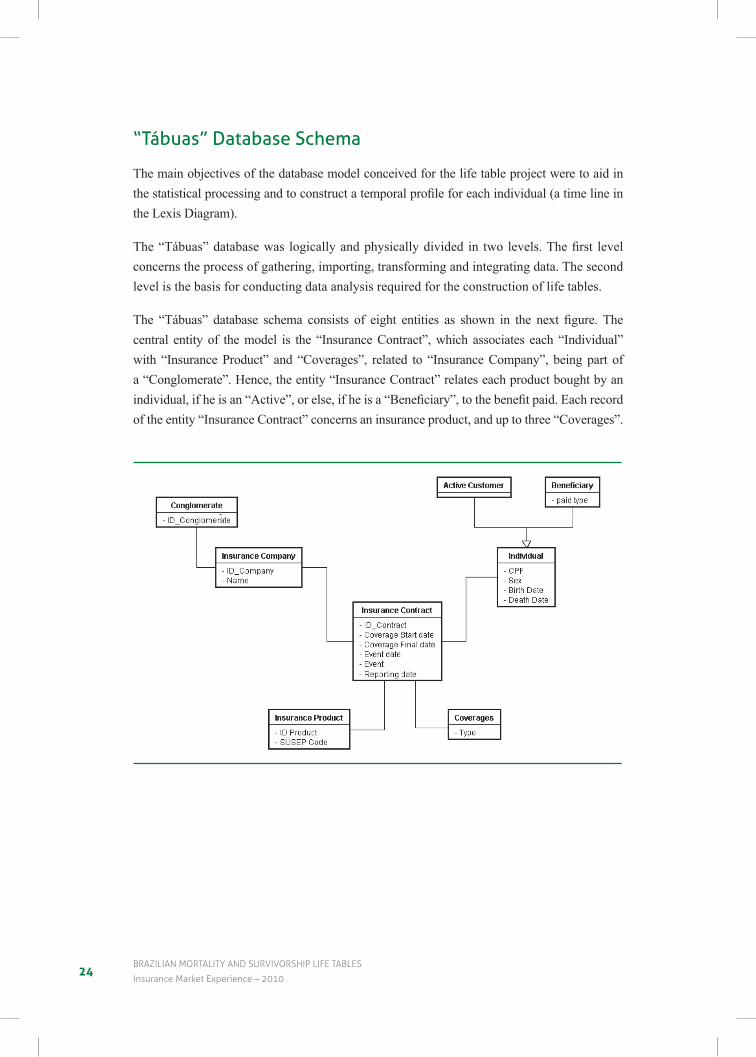
The main objectives of the database model conceived for the life table project were to aid in thestatisticalprocessingandtoconstructatemporalprofileforeachindividual(atimelineinthe Lexis Diagram).
The“Tábuas”databasewas logicallyandphysicallydivided in two levels.Thefirst levelconcerns the process of gathering, importing, transforming and integrating data. The second level is the basis for conducting data analysis required for the construction of life tables.
The “Tábuas” database schema consists of eight entities as shown in the next figure.Thecentral entity of the model is the “Insurance Contract”, which associates each “Individual” with “Insurance Product” and “Coverages”, related to “Insurance Company”, being part of a “Conglomerate”. Hence, the entity “Insurance Contract” relates each product bought by an individual,ifheisan“Active”,orelse,ifheisa“Beneficiary”,tothebenefitpaid.Eachrecordof the entity “Insurance Contract” concerns an insurance product, and up to three “Coverages”.

254 DataBase cOnstructIOn
database integration
The next step is to integrate the various data sets, associated with the numerous insurance companies into a single database. The integration process dealt with heterogeneities among the schemas for the different calendar years. During the process, the most evident problem was related to the fact that the “Insurance Product” list for 2004 was different from that of 2005 and 2006.
Thedataconversionandintegrationprocessesgothroughsuccessivestepsoffilteringandclustering using database views. To implement the integration of the database as a whole, 178 database views were programmed. The highest database view hierarchical level integrates all the data collected from the insurance companies. All data analysis routines run on this database view.
data quality check
In this step a data analysis was performed in order to check the quality of the data gathered. To do that, three different procedures were implemented:
i. Consistencycheckofstocksandflows;
ii. CPF – tax registration ID validation check; and
iii. Population and death age and sex distribution check.
This last check was performed for each combination of calendar year, “Insurance Company”, “Insurance Product” and “Coverage”.
Consistency check of stocks and flows
Inthefirstcheckperformed,stocksandflowswereverifiedforconsistency:stockatthebegin-ning of the year plus new entries should match stock at the end of the year less withdrawals.
This Consistency check was performed for the aggregated database by sex and, later on, tallying by the combination of:
i. Insurance company (23 companies);
ii. Calendar year (2004, 2005 and 2006);
iii.Insuranceproduct(definedbySUSEPin7categories);
iv. Coverage (2 types);
v. Activitystatus(activeorbeneficiary);and
vi. Age.
26BraZILIan mOrtaLItY anD surVIVOrsHIp LIFe taBLes
Insurance market experience – 2010
Thesecondconsistencycheckverifiedinformationinadjacentyears:stockattheendofagiven calendar year should match the stock at the beginning of the following year. This check was performed for the link between 2004 and 2005, and between 2005 and 2006. This consis-tency check was also performed for the aggregated database by sex and, later on, tallying by the same combination described above. These analyses showed some inconsistencies, which were not particularly important for the project.
tax registration id validation check
ThevalidationcheckoftheCPF(taxID)informationwasfirstperformedusingtheinternalconsistency check of the tax ID. The CPF consists of a set of 9 digits followed by 2 control digits.The2controldigitscanbeobtainedasafunctionoftheprevious9digits(IRSdefinesthefunction).Inthevalidationcheck,CPFsthatdidnotconformtothecontroldigitverifica-tion were considered invalid and correspond records were analyzed separately. Afterwards, somecombinationsthatdidconformtothecontroldigitverificationbutwereeasilyrecogniz-able fakes, such as 000.000.001-71, 111.111.111-11, 222.222.222-22, were also considered invalid. In the “Tábuas” database, 13.7% of the registers contained invalid tax ID numbers, which corresponded to less than 0,1% of the individuals of the whole database.
Identification of individuals
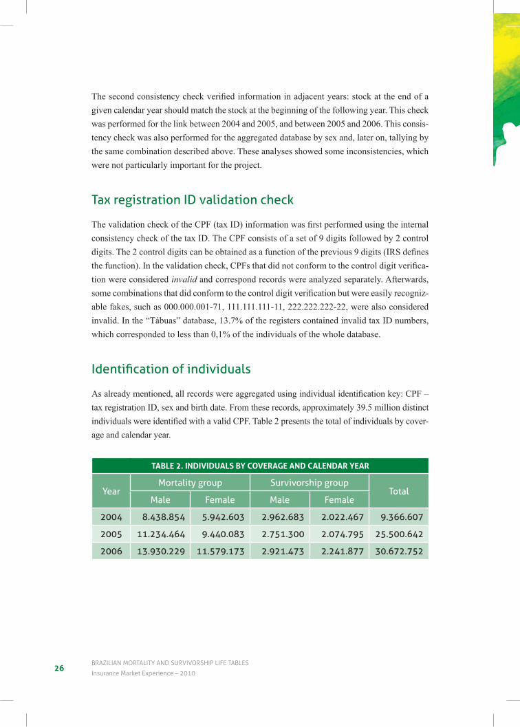
Asalreadymentioned,allrecordswereaggregatedusingindividualidentificationkey:CPF–tax registration ID, sex and birth date. From these records, approximately 39.5 million distinct individualswereidentifiedwithavalidCPF.Table2presentsthetotalofindividualsbycover-age and calendar year.
TABLe 2. InDIvIDuALs By CoverAge AnD CALenDAr yeAr
YearMortality group Survivorship group
totalMale Female Male Female
2004 8.438.854 5.942.603 2.962.683 2.022.467 9.366.607
2005 11.234.464 9.440.083 2.751.300 2.074.795 25.500.642
2006 13.930.229 11.579.173 2.921.473 2.241.877 30.672.752
27
5 selection of subpopulations
5.1 Population distribution and evolution in time
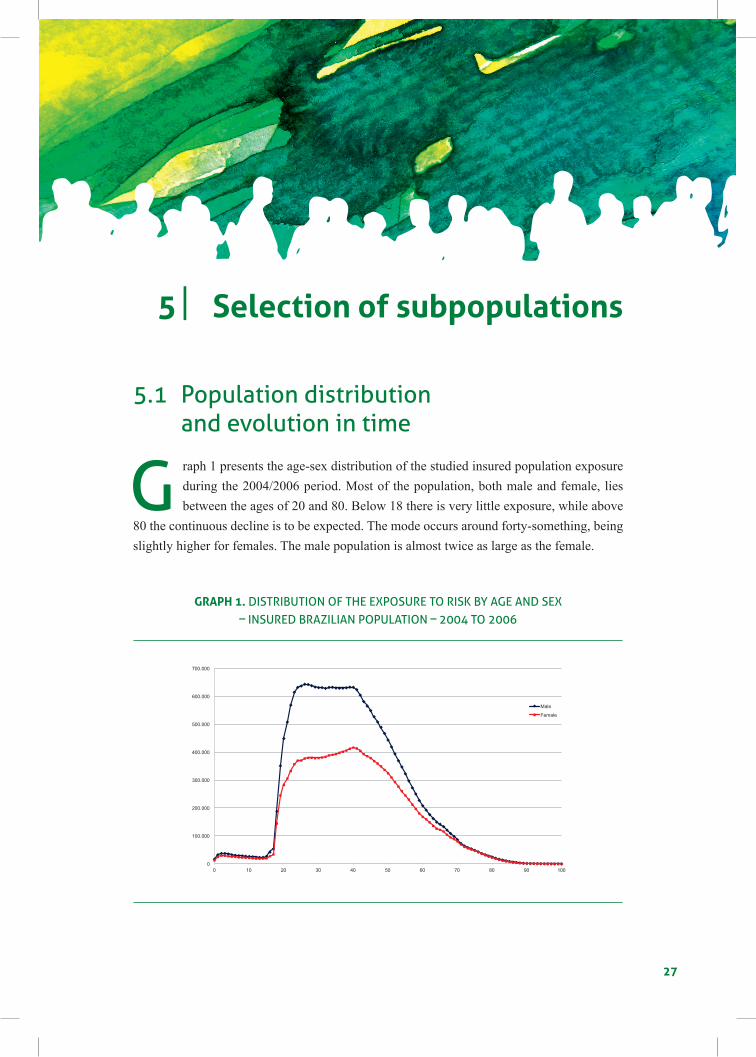
G raph 1 presents the age-sex distribution of the studied insured population exposure during the 2004/2006 period. Most of the population, both male and female, lies between the ages of 20 and 80. Below 18 there is very little exposure, while above
80 the continuous decline is to be expected. The mode occurs around forty-something, being slightly higher for females. The male population is almost twice as large as the female.
grAPH 1. diStriBUtion oF the eXPoSUre to riSk BY aGe and SeX – inSUred Brazilian PoPUlation – 2004 to 2006
0
100.000
200.000
300.000
400.000
500.000
600.000
700.000
0 10 20 30 40 50 60 70 80 90 100
DISTRIBUTION OF THE EXPOSURE TO RISK BY AGE AND SEX – INSURED BRAZILIAN POPULATION – 2004 TO 2006
Male
Female
28BraZILIan mOrtaLItY anD surVIVOrsHIp LIFe taBLes
Insurance market experience – 2010
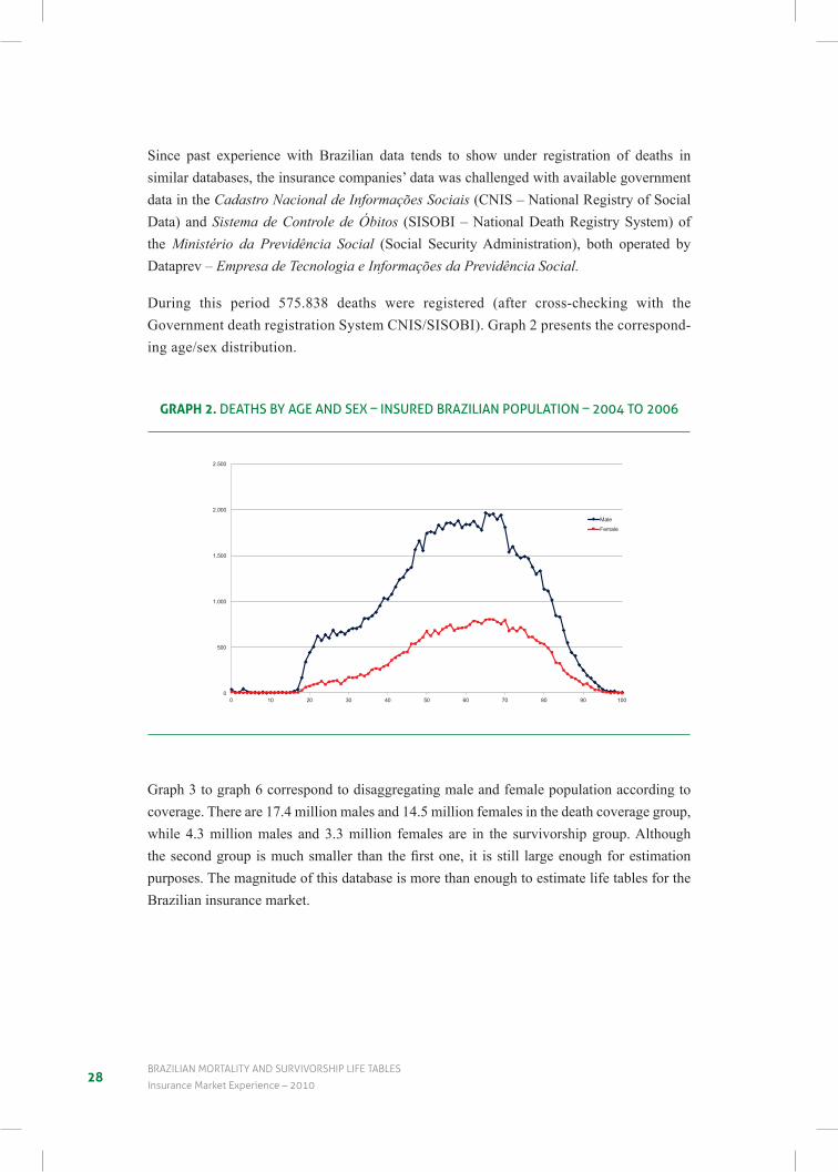
Since past experience with Brazilian data tends to show under registration of deaths in similar databases, the insurance companies’ data was challenged with available government data in the Cadastro Nacional de Informações Sociais (CNIS – National Registry of Social Data) and Sistema de Controle de Óbitos (SISOBI – National Death Registry System) of the Ministério da Previdência Social (Social Security Administration), both operated by Dataprev – Empresa de Tecnologia e Informações da Previdência Social.
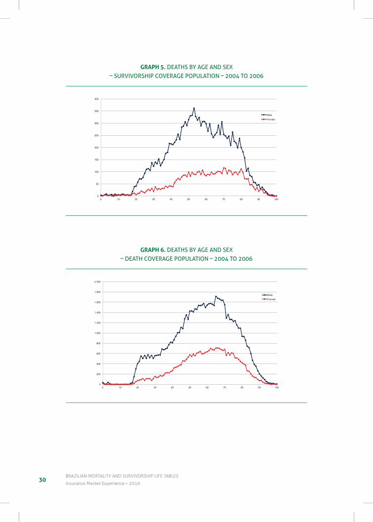
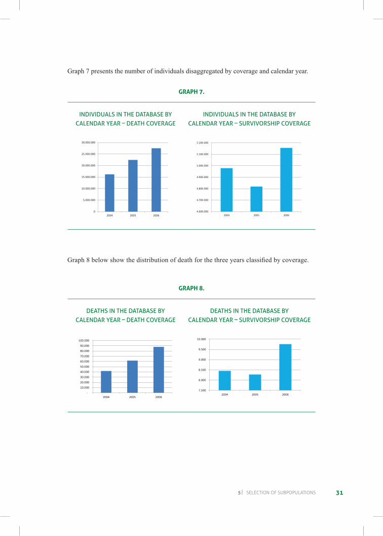
During this period 575.838 deaths were registered (after cross-checking with the Government death registration System CNIS/SISOBI). Graph 2 presents the correspond-ing age/sex distribution.
grAPH 2. deathS BY aGe and SeX – inSUred Brazilian PoPUlation – 2004 to 2006
0
500
1.000
1.500
2.000
2.500
0 10 20 30 40 50 60 70 80 90 100
DEATHS BY AGE AND SEX – INSURED BRAZILIAN POPULATION – 2004 TO 2006
Male
Female
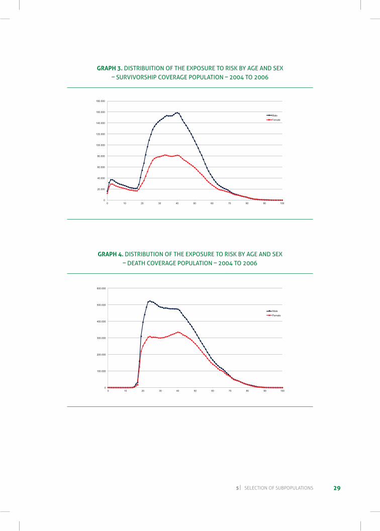
Graph 3 to graph 6 correspond to disaggregating male and female population according to coverage. There are 17.4 million males and 14.5 million females in the death coverage group, while 4.3 million males and 3.3 million females are in the survivorship group. Although thesecondgroupismuchsmaller thanthefirstone, it isstill largeenoughforestimationpurposes. The magnitude of this database is more than enough to estimate life tables for the Brazilian insurance market.
295 seLectIOn OF suBpOpuLatIOns
grAPH 3. diStriBUition oF the eXPoSUre to riSk BY aGe and SeX – SUrvivorShiP coveraGe PoPUlation – 2004 to 2006
0
20.000
40.000
60.000
80.000
100.000
120.000
140.000
160.000
180.000
0 10 20 30 40 50 60 70 80 90 100
DISTRIBUTION OF THE EXPOSURE TO RISK BY AGE AND SEX –SURVIVORSHIP COVERAGE POPULATION – 2004 TO 2006
Male
Female
grAPH 4. diStriBUtion oF the eXPoSUre to riSk BY aGe and SeX – death coveraGe PoPUlation – 2004 to 2006
0
100.000
200.000
300.000
400.000
500.000
600.000
0 10 20 30 40 50 60 70 80 90 100
DISTRIBUTION OF THE EXPOSURE TO RISK BY AGE AND SEX – DEATH COVERAGE POPULATION – 2004 TO 2006
Male
Female
30BraZILIan mOrtaLItY anD surVIVOrsHIp LIFe taBLes
Insurance market experience – 2010
grAPH 5. deathS BY aGe and SeX – SUrvivorShiP coveraGe PoPUlation – 2004 to 2006
0
50
100
150
200
250
300
350
400
0 10 20 30 40 50 60 70 80 90 100
DEATHS BY AGE AND SEX – SURVIVORSHIP COVERAGE POPULATION –2004 TO 2006
Male
Female
grAPH 6. deathS BY aGe and SeX – death coveraGe PoPUlation – 2004 to 2006
0
200
400
600
800
1.000
1.200
1.400
1.600
1.800
2.000
0 10 20 30 40 50 60 70 80 90 100
DEATHS BY AGE AND SEX – DEATH COVERAGE POPULATION – 2004 TO 2006
Male
Female
315 seLectIOn OF suBpOpuLatIOns
Graph 7 presents the number of individuals disaggregated by coverage and calendar year.
grAPH 7.
individUalS in the dataBaSe BY calendar Year – death coveraGe
individUalS in the dataBaSe BY calendar Year – SUrvivorShiP coveraGe
0
5.000.000
10.000.000
15.000.000
20.000.000
25.000.000
30.000.000
2004 2005 2006
INDIVIDUALS IN THE DATABASE BY CALENDAR YEAR - DEATH
COVERAGE
4.600.000
4.700.000
4.800.000
4.900.000
5.000.000
5.100.000
5.200.000
2004 2005 2006
INDIVIDUALS IN THE DATABASE BY CALENDAR YEAR - SURVIVORSHIP
COVERAGE
0
5.000.000
10.000.000
15.000.000
20.000.000
25.000.000
30.000.000
2004 2005 2006
INDIVIDUALS IN THE DATABASE BY CALENDAR YEAR - DEATH
COVERAGE
4.600.000
4.700.000
4.800.000
4.900.000
5.000.000
5.100.000
5.200.000
2004 2005 2006
INDIVIDUALS IN THE DATABASE BY CALENDAR YEAR - SURVIVORSHIP
COVERAGE
Graph8belowshowthedistributionofdeathforthethreeyearsclassifiedbycoverage.
grAPH 8.
deathS in the dataBaSe BY calendar Year – death coveraGe
deathS in the dataBaSe BY calendar Year – SUrvivorShiP coveraGe
-
10.000
20.000
30.000
40.000
50.000
60.000
70.000
80.000
90.000
100.000
2004 2005 2006
DEATHS IN THE DATABASE BY CALENDAR YEAR - DEATH
COVERAGE
7.500
8.000
8.500
9.000
9.500
10.000
2004 2005 2006
DEATHS IN THE DATABASE BY CALENDAR YEAR - SURVIVORSHIP
COVERAGE
-
10.000
20.000
30.000
40.000
50.000
60.000
70.000
80.000
90.000
100.000
2004 2005 2006
DEATHS IN THE DATABASE BY CALENDAR YEAR - DEATH
COVERAGE
7.500
8.000
8.500
9.000
9.500
10.000
2004 2005 2006
DEATHS IN THE DATABASE BY CALENDAR YEAR - SURVIVORSHIP
COVERAGE
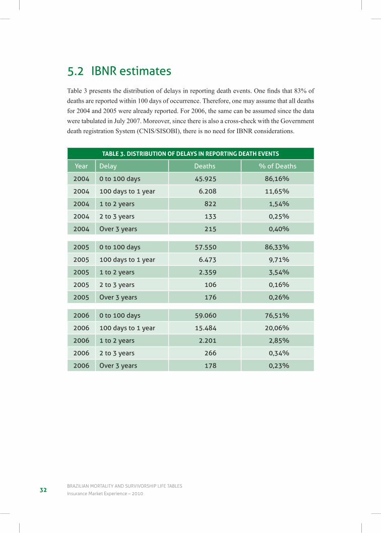
32BraZILIan mOrtaLItY anD surVIVOrsHIp LIFe taBLes
Insurance market experience – 2010
5.2 iBnr estimatesTable3presentsthedistributionofdelaysinreportingdeathevents.Onefindsthat83%ofdeaths are reported within 100 days of occurrence. Therefore, one may assume that all deaths for 2004 and 2005 were already reported. For 2006, the same can be assumed since the data were tabulated in July 2007. Moreover, since there is also a cross-check with the Government death registration System (CNIS/SISOBI), there is no need for IBNR considerations.
TABLe 3. DIsTrIBuTIon of DeLAys In rePorTIng DeATH evenTs
Year delay deaths % of deaths
2004 0 to 100 days 45.925 86,16%
2004 100 days to 1 year 6.208 11,65%
2004 1 to 2 years 822 1,54%
2004 2 to 3 years 133 0,25%
2004 over 3 years 215 0,40%
2005 0 to 100 days 57.550 86,33%
2005 100 days to 1 year 6.473 9,71%
2005 1 to 2 years 2.359 3,54%
2005 2 to 3 years 106 0,16%
2005 over 3 years 176 0,26%
2006 0 to 100 days 59.060 76,51%
2006 100 days to 1 year 15.484 20,06%
2006 1 to 2 years 2.201 2,85%
2006 2 to 3 years 266 0,34%
2006 over 3 years 178 0,23%
335 seLectIOn OF suBpOpuLatIOns
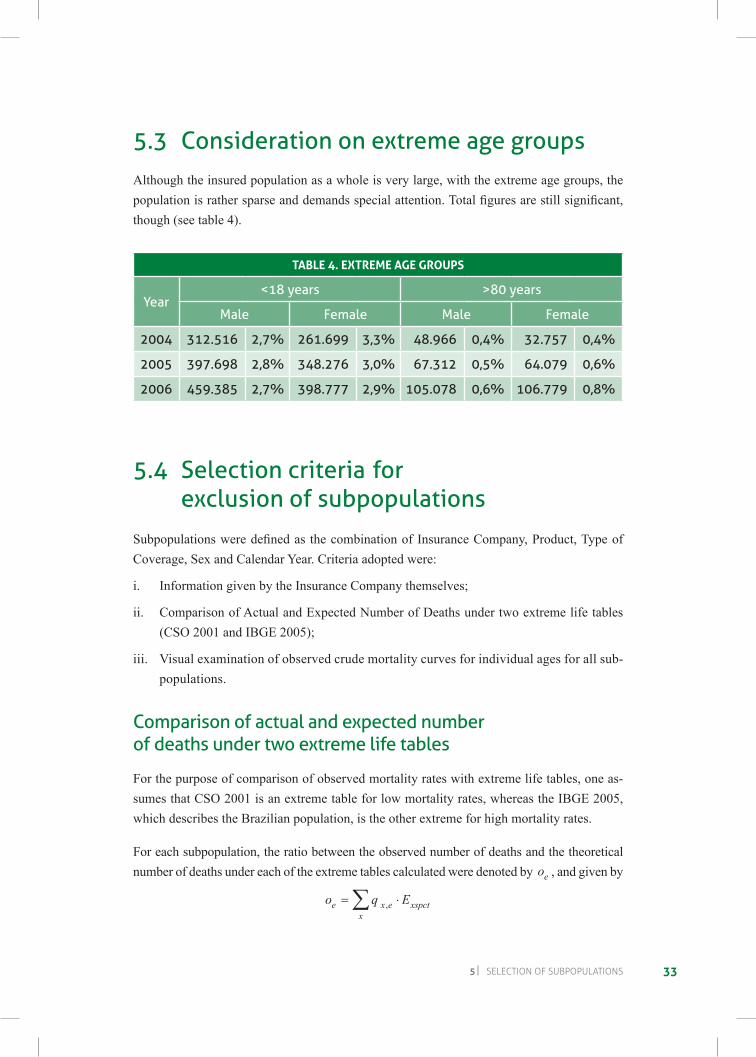
5.3 consideration on extreme age groupsAlthough the insured population as a whole is very large, with the extreme age groups, the populationisrathersparseanddemandsspecialattention.Totalfiguresarestillsignificant,though (see table 4).
TABLe 4. exTreMe Age grouPs
Year<18 years >80 years
Male Female Male Female
2004 312.516 2,7% 261.699 3,3% 48.966 0,4% 32.757 0,4%
2005 397.698 2,8% 348.276 3,0% 67.312 0,5% 64.079 0,6%
2006 459.385 2,7% 398.777 2,9% 105.078 0,6% 106.779 0,8%
5.4 Selection criteria for exclusion of subpopulations
SubpopulationsweredefinedasthecombinationofInsuranceCompany,Product,TypeofCoverage, Sex and Calendar Year. Criteria adopted were:
i. Information given by the Insurance Company themselves;
ii. Comparison of Actual and Expected Number of Deaths under two extreme life tables (CSO 2001 and IBGE 2005);
iii. Visual examination of observed crude mortality curves for individual ages for all sub-populations.
comparison of actual and expected numberof deaths under two extreme life tables
For the purpose of comparison of observed mortality rates with extreme life tables, one as-sumes that CSO 2001 is an extreme table for low mortality rates, whereas the IBGE 2005, which describes the Brazilian population, is the other extreme for high mortality rates.
For each subpopulation, the ratio between the observed number of deaths and the theoretical number of deaths under each of the extreme tables calculated were denoted by oe , and given by
o q Ee x ex
xspct= ⋅∑ ,

34BraZILIan mOrtaLItY anD surVIVOrsHIp LIFe taBLes
Insurance market experience – 2010
where qx,e is the probability of death at age x of the extreme table e and Exspct denotes the number of persons with age x, sex s, coverage c in insurance product p at time t. With ratios sodefined,oneassuresthatthereisalwaysapositivevalueforthedenominator.Forsubpop-ulations with high mortality rates, close to the IBGE 2005 table, the ratio relative to IBGE should be close to unity and close to 10 (for men) and 5 (for women) when one considers the CSO 2001, since these are the average values of the ratios of probability of death between CSO and IBGE.
On the other hand, for subpopulations with low mortality rates, close to the CSO 2001 table, the ratio of actual to expected number of deaths should be close to the unity, whereas they are close to 1/10 (for men) and 1/5 (for women) when the IBGE table is considered.
These ratios were plotted in an x-y graph, with the ratio relative to IBGE in the x-axis and the ratio relative to CSO in the y-axis. One should expect, roughly, in the event all subpopula-tions were submitted to the same mortality pattern, that all points should be in a cloud around a central point, close to each other, probably close to a straight line. Points far away from the central point of the cloud should be discharged, since they would probably involve data errors and could bias the results.
Since the numerator of each fraction is the actual number of deaths for each subpopulation, and since the number of deaths, considered as a random variable, is the sum of independent binomial random variables, one for each age, one may assume that the numerator of each fraction will be approximately normally distributed. Therefore, inspired by Tukey (1977), onecancalculateboundsthatwilldefinesubpopulationoutliers.Forthepresentcase,allsub-populations outside these bounds were discharged. The process of establishing bounds and not considering subpopulation outliers was carried on interactively until no further outliers existed. Each bound was established by adding and subtracting 1.5 interquartile distance to the median, thus leaving roughly 95% of the points inside.
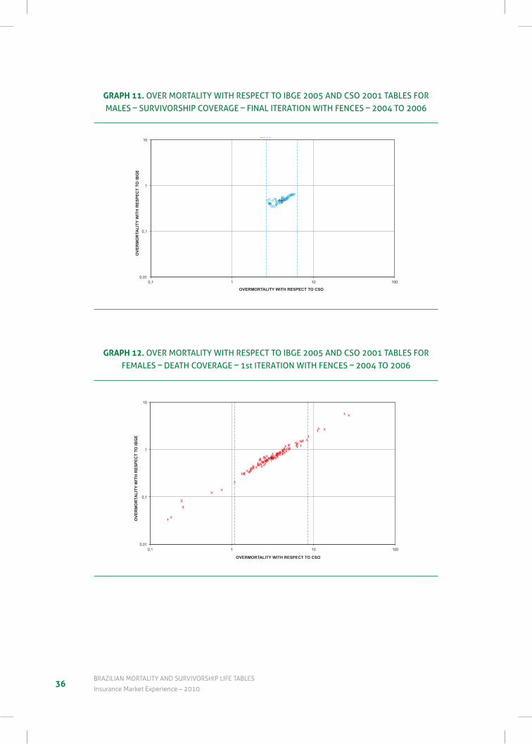
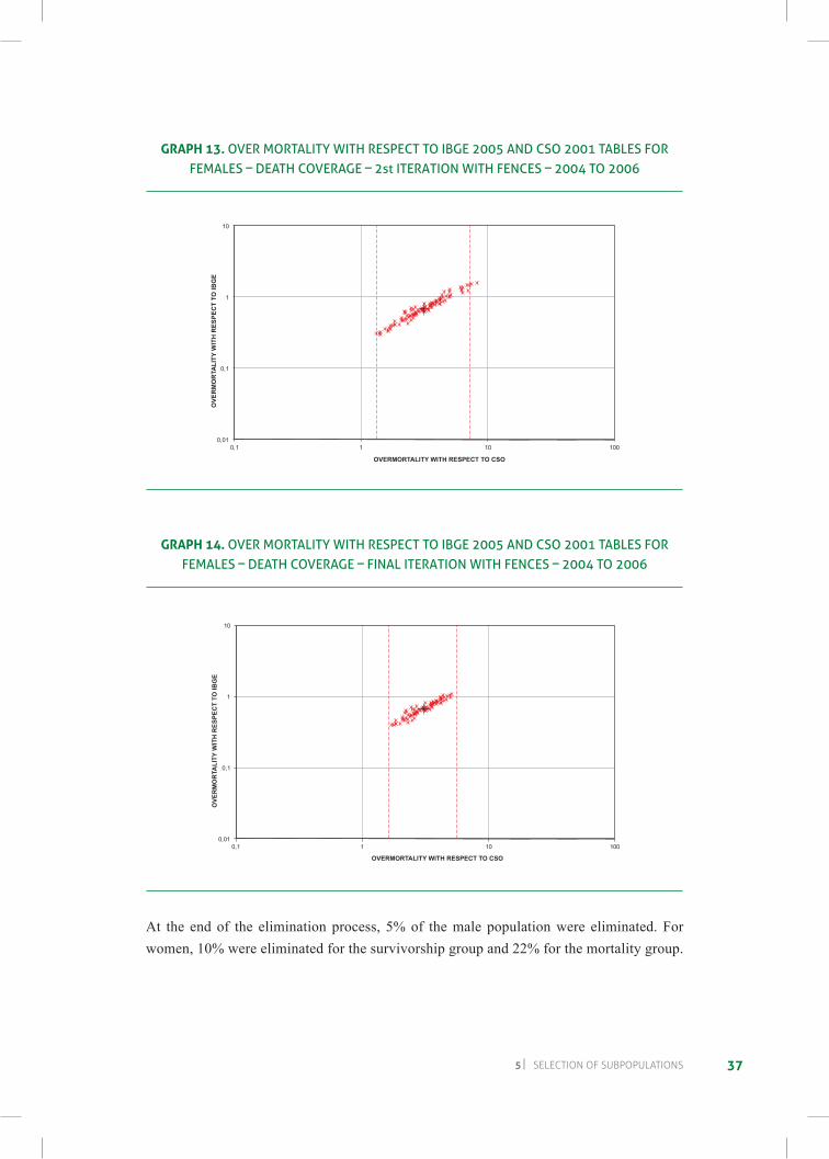
The graphs below present over mortality calculated with respect to the IBGE 2005 and CSO 2001 tables for subpopulations with death and survivorship coverage according to sex and calendar year. In these graphs, crosses indicate medians and the bounds are designated as dashed lines. These graphs do not show any temporal evolution in mortality.
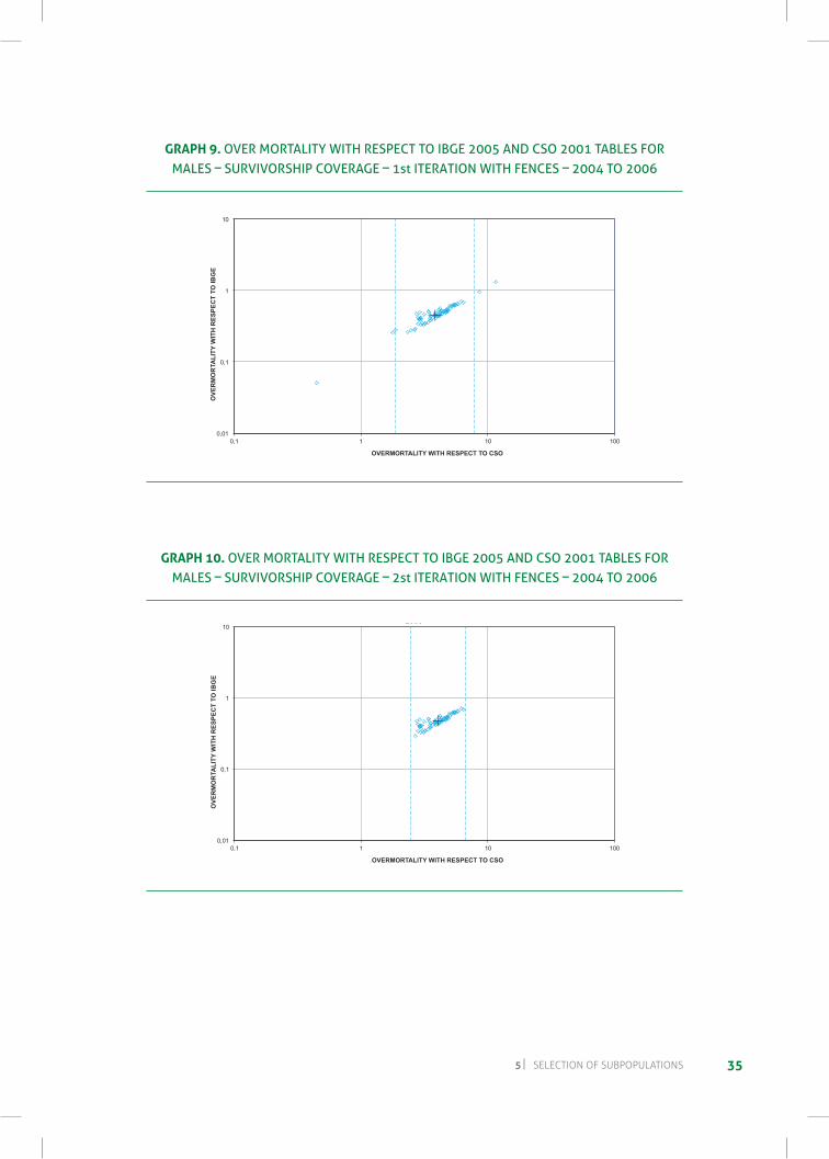
355 seLectIOn OF suBpOpuLatIOns
grAPH 9. over MortalitY With reSPect to iBGe 2005 and cSo 2001 taBleS For MaleS – SUrvivorShiP coveraGe – 1st iteration With FenceS – 2004 to 2006
0,01
0,1
1
10
0,1 1 10 100
OVE
R M
ORT
ALIT
Y W
ITH
RESP
ECT
TO C
SO
OVER MORTALITY WITH RESPECT TO IBGE
OVER MORTALITY WITH RESPECT TO IBGE 2005 AND CSO 2001 TABLES FOR MALES – SURVIVORSHIP COVERAGE – 1st ITERATION WITH FENCES – 2004 TO
2006O
VER
MO
RTA
LITY
WIT
H R
ESPE
CT
TO IB
GE
OVERMORTALITY WITH RESPECT TO CSO
grAPH 10. over MortalitY With reSPect to iBGe 2005 and cSo 2001 taBleS For MaleS – SUrvivorShiP coveraGe – 2st iteration With FenceS – 2004 to 2006
0,01
0,1
1
10
0,1 1 10 100
OVE
R M
ORT
ALIT
Y W
ITH
RESP
ECT
TO C
SO
OVER MORTALITY WITH RESPECT TO IBGE
OVER MORTALITY WITH RESPECT TO IBGE 2005 AND CSO 2001 TABLES FOR MALES – SURVIVORSHIP COVERAGE – 2nd ITERATION WITH FENCES – 2004 TO
2006
OVE
RM
OR
TALI
TY W
ITH
RES
PEC
T TO
IBG
E
OVERMORTALITY WITH RESPECT TO CSO
36BraZILIan mOrtaLItY anD surVIVOrsHIp LIFe taBLes
Insurance market experience – 2010
grAPH 11. over MortalitY With reSPect to iBGe 2005 and cSo 2001 taBleS For MaleS – SUrvivorShiP coveraGe – Final iteration With FenceS – 2004 to 2006
0,01
0,1
1
10
0,1 1 10 100
OVE
R M
ORT
ALIT
Y W
ITH
RESP
ECT
TO C
SO
OVER MORTALITY WITH RESPECT TO IBGE
OVER MORTALITY WITH RESPECT TO IBGE 2005 AND CSO 2001 TABLES FOR MALES – SURVIVORSHIP COVERAGE – FINAL ITERATION WITH FENCES – 2004 TO
2006O
VER
MO
RTA
LITY
WIT
H R
ESPE
CT
TO IB
GE
OVERMORTALITY WITH RESPECT TO CSO
grAPH 12. over MortalitY With reSPect to iBGe 2005 and cSo 2001 taBleS For FeMaleS – death coveraGe – 1st iteration With FenceS – 2004 to 2006
0,01
0,1
1
10
0,1 1 10 100
OV
ER
MO
RTA
LITY
WIT
H R
ES
PE
CT
TO C
SO
OVER MORTALITY WITH RESPECT TO IBGE
OVER MORTALITY WITH RESPECT TO IBGE 2005 AND CSO 2001 TABLES FOR FEMALES –DEATH COVERAGE – 1st ITERATION WITH FENCES – 2004 TO 2006
OVE
RM
OR
TALI
TY W
ITH
RES
PEC
T TO
IBG
E
OVERMORTALITY WITH RESPECT TO CSO
375 seLectIOn OF suBpOpuLatIOns
grAPH 13. over MortalitY With reSPect to iBGe 2005 and cSo 2001 taBleS For FeMaleS – death coveraGe – 2st iteration With FenceS – 2004 to 2006
0,01
0,1
1
10
0,1 1 10 100
OVE
R M
ORT
ALIT
Y W
ITH
RESP
ECT
TO C
SO
OVER MORTALITY WITH RESPECT TO IBGE
OVER MORTALITY WITH RESPECT TO IBGE 2005 AND CSO 2001 TABLES FOR FEMALES – DEATH COVERAGE – 2nd ITERATION WITH FENCES – 2004 TO 2006
OVE
RM
OR
TALI
TY W
ITH
RES
PEC
T TO
IBG
E
OVERMORTALITY WITH RESPECT TO CSO
grAPH 14. over MortalitY With reSPect to iBGe 2005 and cSo 2001 taBleS For FeMaleS – death coveraGe – Final iteration With FenceS – 2004 to 2006
0,01
0,1
1
10
0,1 1 10 100
OVE
R M
ORT
ALIT
Y W
ITH
RESP
ECT
TO C
SO
OVER MORTALITY WITH RESPECT TO IBGE
OVER MORTALITY WITH RESPECT TO IBGE 2005 AND CSO 2001 TABLES FOR FEMALES – DEATH COVERAGE – FINAL ITERATION WITH FENCES – 2004 TO 2006
OVE
RM
OR
TALI
TY W
ITH
RES
PEC
T TO
IBG
E
OVERMORTALITY WITH RESPECT TO CSO
At the end of the elimination process, 5% of the male population were eliminated. For women, 10% were eliminated for the survivorship group and 22% for the mortality group.
38BraZILIan mOrtaLItY anD surVIVOrsHIp LIFe taBLes
Insurance market experience – 2010
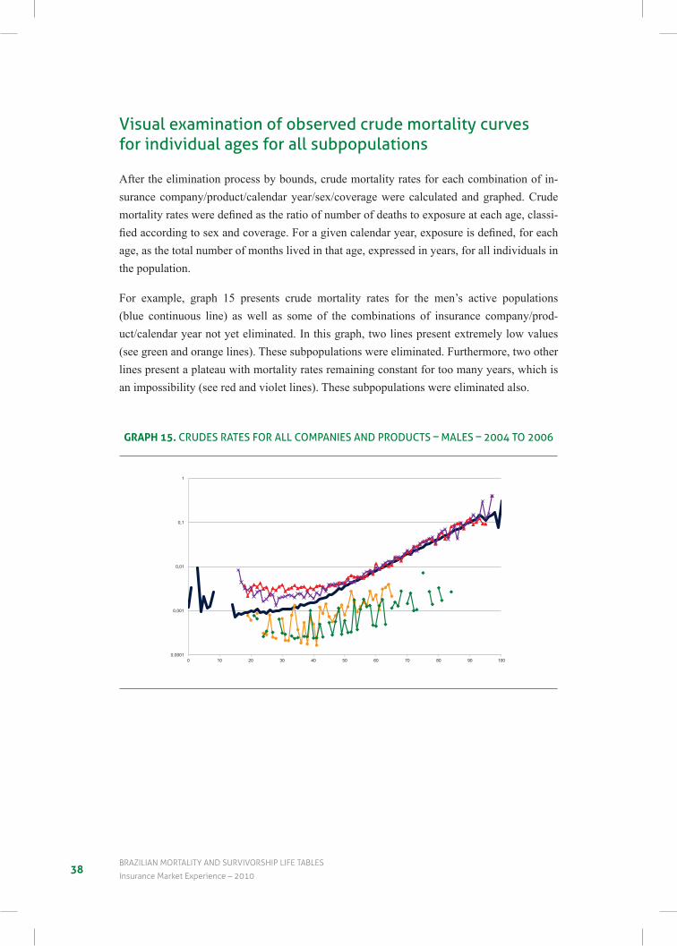
visual examination of observed crude mortality curvesfor individual ages for all subpopulations
After the elimination process by bounds, crude mortality rates for each combination of in-surance company/product/calendar year/sex/coverage were calculated and graphed. Crude mortalityratesweredefinedastheratioofnumberofdeathstoexposureateachage,classi-fiedaccordingtosexandcoverage.Foragivencalendaryear,exposureisdefined,foreachage, as the total number of months lived in that age, expressed in years, for all individuals in the population.
For example, graph 15 presents crude mortality rates for the men’s active populations (blue continuous line) as well as some of the combinations of insurance company/prod-uct/calendar year not yet eliminated. In this graph, two lines present extremely low values (see green and orange lines). These subpopulations were eliminated. Furthermore, two other lines present a plateau with mortality rates remaining constant for too many years, which is an impossibility (see red and violet lines). These subpopulations were eliminated also.
grAPH 15. crUdeS rateS For all coMPanieS and ProdUctS – MaleS – 2004 to 2006
0,0001
0,001
0,01
0,1
1
0 10 20 30 40 50 60 70 80 90 100
CRUDE RATES FOR ALL COMPANIES AND PRODUCTS – MALES –2004 TO 2006
395 seLectIOn OF suBpOpuLatIOns
5.5 Differentiation of mortality curves according to sex and coverage
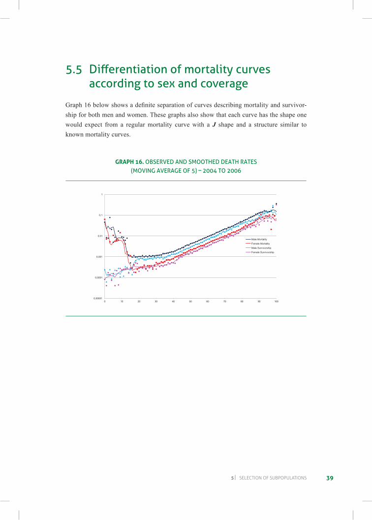
Graph16belowshowsadefiniteseparationofcurvesdescribingmortalityandsurvivor-ship for both men and women. These graphs also show that each curve has the shape one would expect from a regular mortality curve with a J shape and a structure similar to known mortality curves.
grAPH 16. oBServed and SMoothed death rateS (MovinG averaGe oF 5) – 2004 to 2006
0,00001
0,0001
0,001
0,01
0,1
1
0 10 20 30 40 50 60 70 80 90 100
OBSERVED AND SMOOTHED DEATH RATES (MOVING AVERAGE OF 5) – 2004 TO 2006
Male Mortality
Female Mortality
Male Survivorship
Female Survivorship
40BraZILIan mOrtaLItY anD surVIVOrsHIp LIFe taBLes
Insurance market experience – 2010
Men
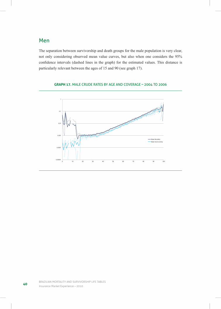
The separation between survivorship and death groups for the male population is very clear, not only considering observed mean value curves, but also when one considers the 95% confidence intervals (dashed lines in thegraph) for theestimatedvalues.Thisdistance isparticularly relevant between the ages of 15 and 90 (see graph 17).
grAPH 17. Male crUde rateS BY aGe and coveraGe – 2004 to 2006
0,00001
0,0001
0,001
0,01
0,1
1
0 10 20 30 40 50 60 70 80 90 100
MALE CRUDE RATES BY AGE AND COVERAGE – 2004 TO 2006
Male Mortality
Male Survivorship
415 seLectIOn OF suBpOpuLatIOns
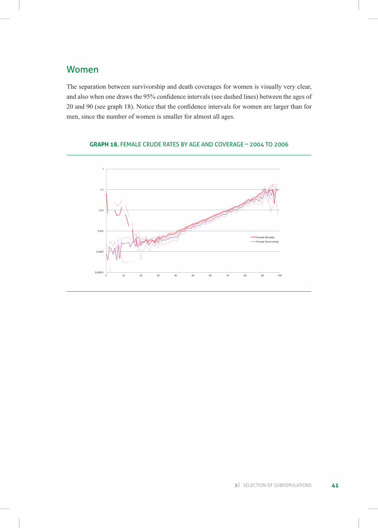
Women
The separation between survivorship and death coverages for women is visually very clear, andalsowhenonedrawsthe95%confidenceintervals(seedashedlines)betweentheagesof20and90(seegraph18).Noticethattheconfidenceintervalsforwomenarelargerthanformen, since the number of women is smaller for almost all ages.
grAPH 18. FeMale crUde rateS BY aGe and coveraGe – 2004 to 2006
0,00001
0,0001
0,001
0,01
0,1
1
0 10 20 30 40 50 60 70 80 90 100
FEMALE CRUDE RATES BY AGE AND COVERAGE – 2004 TO 2006
Female Mortality
Female Survivorship
42BraZILIan mOrtaLItY anD surVIVOrsHIp LIFe taBLes
Insurance market experience – 2010
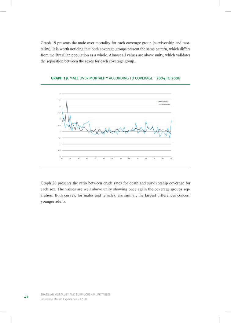
Graph 19 presents the male over mortality for each coverage group (survivorship and mor-tality). It is worth noticing that both coverage groups present the same pattern, which differs from the Brazilian population as a whole. Almost all values are above unity, which validates the separation between the sexes for each coverage group.
grAPH 19. Male over MortalitY accordinG to coveraGe – 2004 to 2006
0
0,5
1
1,5
2
2,5
3
3,5
4
4,5
5
25 30 35 40 45 50 55 60 65 70 75 80 85 90
MALE OVER MORTALITY ACCORDING TO COVERAGE – 2004 TO 2006
Mortality
Survivorship
Graph 20 presents the ratio between crude rates for death and survivorship coverage for each sex. The values are well above unity showing once again the coverage groups sep-aration. Both curves, for males and females, are similar; the largest differences concern younger adults.
435 seLectIOn OF suBpOpuLatIOns
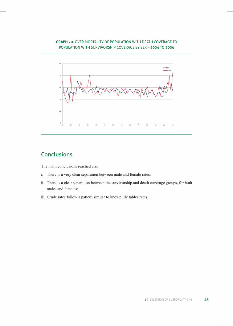
grAPH 20. over MortalitY oF PoPUlation With death coveraGe to PoPUlation With SUrvivorShiP coveraGe BY SeX – 2004 to 2006
0
0,5
1
1,5
2
2,5
25 30 35 40 45 50 55 60 65 70 75 80 85 90
OVER MORTALITY OF POPULATION WITH DEATH COVERAGE TO POPULATION WITH SURVIVORSHIP COVERAGE BY SEX – 2004 TO 2006
Male
Female
conclusions
The main conclusions reached are:
i. There is a very clear separation between male and female rates;
ii. There is a clear separation between the survivorship and death coverage groups, for both males and females;
iii. Crude rates follow a pattern similar to known life tables rates.


45
6 Construction of Lifeand survival Tables
6.1 heligman & Pollard model
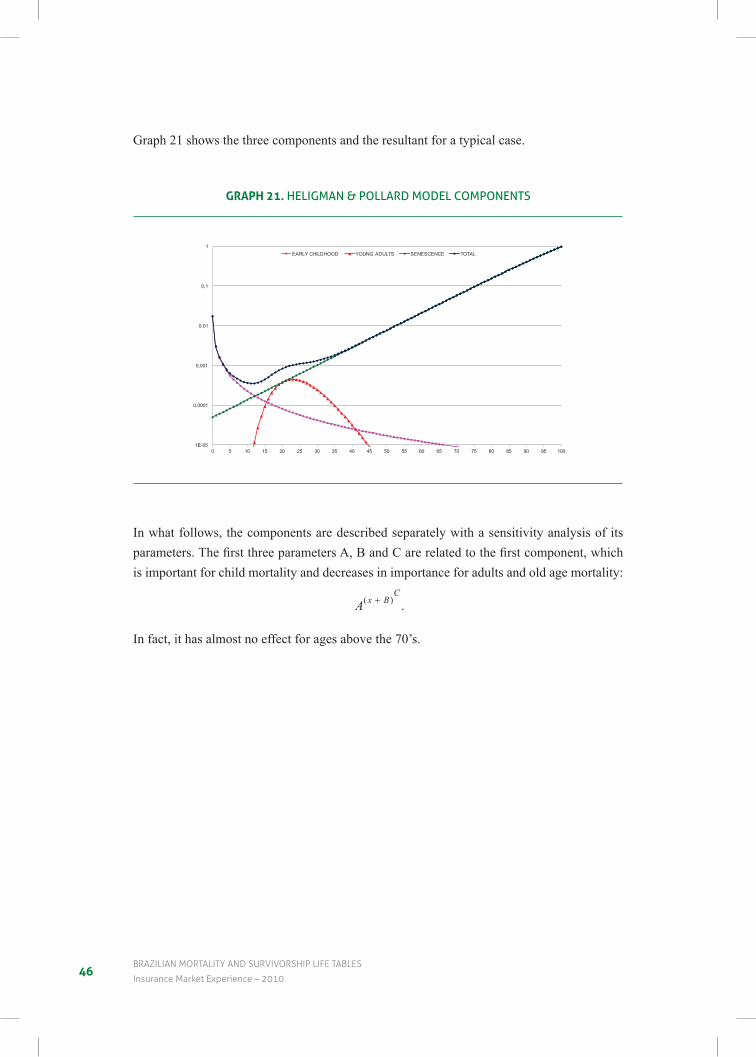
t he model proposed by Heligman & Pollard (1980) has three components: child mortality, a “hump” for young adult mortality and a component for middle and old age mortality:
q x A DeGH
KGH
x BC
E x Fx
x( )
( )
( ) (ln ln )= + ++
+ − −2
1.
The Heligman & Pollard model can be viewed as a combination of different parametric models for describing human mortality. The second component is particularly useful for de-scribing the mortality of young adults by external causes, a phenomenon which has been increasing since the middle of last century.
Sincethemodelhasnineparametersfor the threecomponents, it isveryflexibleandcanapproximate almost all known human mortality experiences. For these reasons, the Heligman & Pollard model was chosen for construction of mortality and survival tables.
46BraZILIan mOrtaLItY anD surVIVOrsHIp LIFe taBLes
Insurance market experience – 2010
Graph 21 shows the three components and the resultant for a typical case.
grAPH 21. heliGMan & Pollard Model coMPonentS
1E-05
0,0001
0,001
0,01
0,1
1
0 5 10 15 20 25 30 35 40 45 50 55 60 65 70 75 80 85 90 95 100
HELIGMAN & POLLARD MODEL COMPONENTS
EARLY CHILDHOOD YOUNG ADULTS SENESCENCE TOTAL
In what follows, the components are described separately with a sensitivity analysis of its parameters.ThefirstthreeparametersA,BandCarerelatedtothefirstcomponent,whichis important for child mortality and decreases in importance for adults and old age mortality:
A x BC
( )+ .
In fact, it has almost no effect for ages above the 70’s.
476 cOnstructIOn OF LIFe anD surVIVaL taBLes
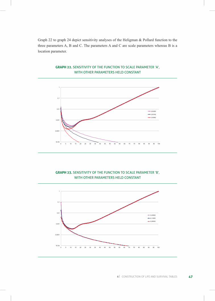
Graph 22 to graph 24 depict sensitivity analyses of the Heligman & Pollard function to the three parameters A, B and C. The parameters A and C are scale parameters whereas B is a location parameter.
grAPH 22. SenSitivitY oF the FUnction to Scale ParaMeter ‘a’, With other ParaMeterS held conStant
1E-05
0,0001
0,001
0,01
0,1
1
0 5 10 15 20 25 30 35 40 45 50 55 60 65 70 75 80 85 90 95 100
SENSITIVITY OF THE FUNCTION TO SCALE PARAMETER ‘A’ WITH OTHER PARAMETERS HELD CONSTANT
0,00282
0,00182
0,00082
grAPH 23. SenSitivitY oF the FUnction to Scale ParaMeter ‘B’, With other ParaMeterS held conStant
1E-05
0,0001
0,001
0,01
0,1
1
0 5 10 15 20 25 30 35 40 45 50 55 60 65 70 75 80 85 90 95 100
SENSITIVITY OF THE FUNCTION TO SCALE PARAMETER ‘B’ WITH OTHER PARAMETERS HELD CONSTANT
0,00500
0,13000
0,80000
48BraZILIan mOrtaLItY anD surVIVOrsHIp LIFe taBLes
Insurance market experience – 2010
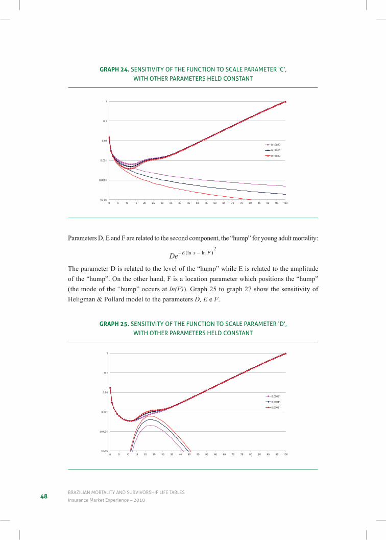
grAPH 24. SenSitivitY oF the FUnction to Scale ParaMeter ‘c’, With other ParaMeterS held conStant
1E-05
0,0001
0,001
0,01
0,1
1
0 5 10 15 20 25 30 35 40 45 50 55 60 65 70 75 80 85 90 95 100
SENSITIVITY OF THE FUNCTION TO SCALE PARAMETER ‘C’ WITH OTHER PARAMETERS HELD CONSTANT
0,12020
0,14020
0,16020
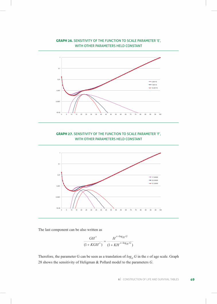
Parameters D, E and F are related to the second component, the “hump” for young adult mortality:
De E x F− −(ln ln )2
The parameter D is related to the level of the “hump” while E is related to the amplitude of the “hump”. On the other hand, F is a location parameter which positions the “hump” (the mode of the “hump” occurs at ln(F)). Graph 25 to graph 27 show the sensitivity of Heligman & Pollard model to the parameters D, E e F.
grAPH 25. SenSitivitY oF the FUnction to Scale ParaMeter ‘d’, With other ParaMeterS held conStant
1E-05
0,0001
0,001
0,01
0,1
1
0 5 10 15 20 25 30 35 40 45 50 55 60 65 70 75 80 85 90 95 100
SENSITIVITY OF THE FUNCTION TO SCALE PARAMETER ‘D’ WITH OTHER PARAMETERS HELD CONSTANT
0,00021
0,00041
0,00061
496 cOnstructIOn OF LIFe anD surVIVaL taBLes
grAPH 26. SenSitivitY oF the FUnction to Scale ParaMeter ‘e’, With other ParaMeterS held conStant
1E-05
0,0001
0,001
0,01
0,1
1
0 5 10 15 20 25 30 35 40 45 50 55 60 65 70 75 80 85 90 95 100
SENSITIVITY OF THE FUNCTION TO SCALE PARAMETER ‘E’ WITH OTHER PARAMETERS HELD CONSTANT
2,65110
7,65110
12,65110
grAPH 27. SenSitivitY oF the FUnction to Scale ParaMeter ‘F’, With other ParaMeterS held conStant
1E-05
0,0001
0,001
0,01
0,1
1
0 5 10 15 20 25 30 35 40 45 50 55 60 65 70 75 80 85 90 95 100
SENSITIVITY OF THE FUNCTION TO SCALE PARAMETER ‘F’ WITH OTHER PARAMETERS HELD CONSTANT
17,20000
22,20000
27,20000
The last component can be also written as
GHKGH
H
KH
x
x
x H G
x H G( ) ( )
log
log1 1+=
+
+
+
Therefore, the parameter G can be seen as a translation of logH G in the x of age scale. Graph 28 shows the sensitivity of Heligman & Pollard model to the parameters G.
50BraZILIan mOrtaLItY anD surVIVOrsHIp LIFe taBLes
Insurance market experience – 2010
grAPH 28. SenSitivitY oF the FUnction to Scale ParaMeter ‘G’, With other ParaMeterS held conStant
1E-05
0,0001
0,001
0,01
0,1
1
0 5 10 15 20 25 30 35 40 45 50 55 60 65 70 75 80 85 90 95 100
SENSITIVITY OF THE FUNCTION TO SCALE PARAMETER ‘G’ WITH OTHER PARAMETERS HELD CONSTANT
0,00005
0,00006
0,00007
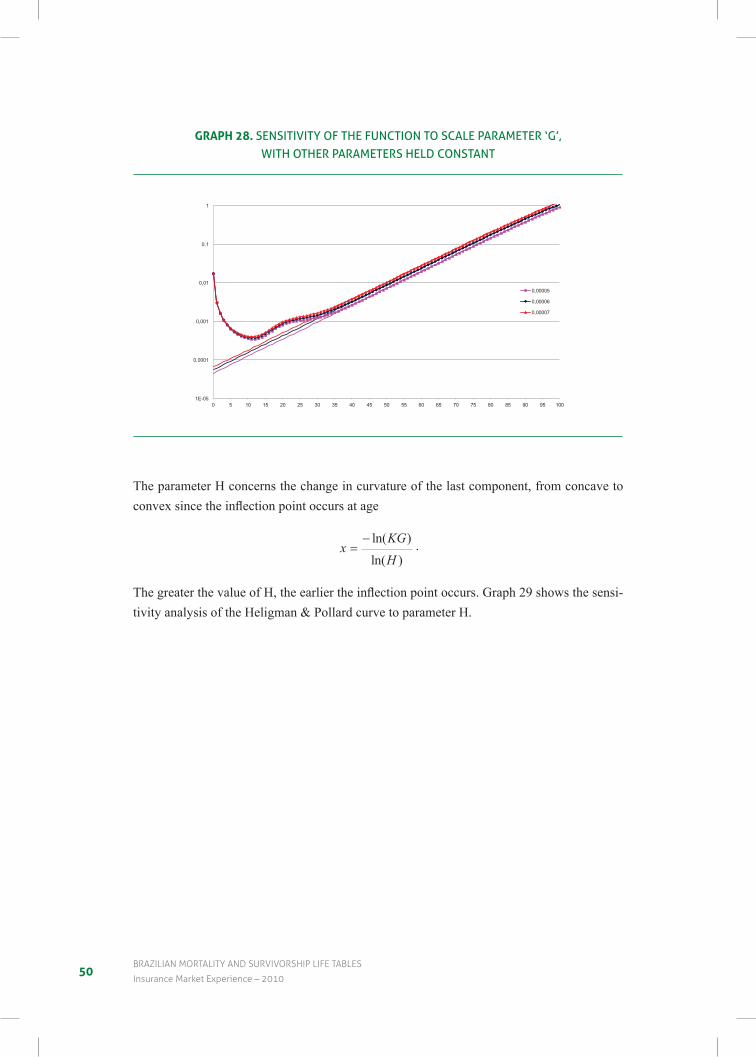
The parameter H concerns the change in curvature of the last component, from concave to convexsincetheinflectionpointoccursatage
xKGH
=− ln( )
ln( ).
ThegreaterthevalueofH,theearliertheinflectionpointoccurs.Graph29showsthesensi-tivity analysis of the Heligman & Pollard curve to parameter H.
516 cOnstructIOn OF LIFe anD surVIVaL taBLes
grAPH 29. SenSitivitY oF the FUnction to Scale ParaMeter ‘h’, With other ParaMeterS held conStant
1E-05
0,0001
0,001
0,01
0,1
1
0 5 10 15 20 25 30 35 40 45 50 55 60 65 70 75 80 85 90 95 100
SENSITIVITY OF THE FUNCTION TO SCALE PARAMETER ‘H’ WITH OTHER PARAMETERS HELD CONSTANT
1,08500
1,09500
1,10500
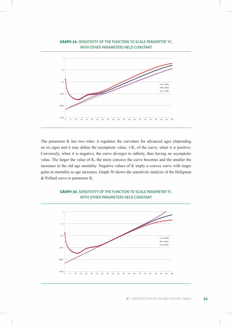
The parameter K has two roles: it regulates the curvature for advanced ages (depending onitssign)anditmaydefinetheasymptoticvalue,1/K,ofthecurve,whenitispositive.Conversely,when it isnegative, thecurvediverges to infinity, thushavingnoasymptoticvalue. The larger the value of K, the more concave the curve becomes and the smaller the increases in the old age mortality. Negative values of K imply a convex curve with larger gains in mortality as age increases. Graph 30 shows the sensitivity analysis of the Heligman & Pollard curve to parameter K.
grAPH 30. SenSitivitY oF the FUnction to Scale ParaMeter ‘k’, With other ParaMeterS held conStant
1E-05
0,0001
0,001
0,01
0,1
1
0 5 10 15 20 25 30 35 40 45 50 55 60 65 70 75 80 85 90 95 100
SENSITIVITY OF THE FUNCTION TO SCALE PARAMETER ‘K’ WITH OTHER PARAMETERS HELD CONSTANT
-0,50000
1,00000
4,00000
52BraZILIan mOrtaLItY anD surVIVOrsHIp LIFe taBLes
Insurance market experience – 2010
6.2. Methodology for the parameters estimation
For a given age x, the number of deaths can be seen as a random variable with binomial dis-tribution B(Nx, qx ), with parameters Nx and qx, where Nx is the number of individuals in the population with age x and qx is the probability of death at age x. The unknown parameter is qx which is to be estimated using the Heligman & Pollard (1980) model.
The estimation problem consists in finding the parameter valueswhichminimize thequadratic objective function
q x q
q xc so
c s khp
x
c s khp
x
, , , ( )
, ,
( )
var ( )
−( )( )∑
2
where
q xc so, ( ) is the observed value for the subpopulation of age x, sex and coverage;
q xc s khp, , ( ) is the adjusted Heligman & Pollard value for the subpopulation of age x, sex and
coverage, at iteration k; and
var( q xc s khp, , ( ) ) is the variance of the corresponding Heligman & Pollard estimate.
According to the binomial hypothesis, this variance is given by
var( ( ))( )( ( ))
, ,, , , ,
, ,
q xq x q x
Nc s khp c s k
hpc s khp
x c s
=−1
where Nx,c,s is the number of individuals in the population with age x, coverage c and sex s.
This is a non-linear regression problem with weights depending on the parameter values to be estimated. This problem has to be solved iteratively: at each step k, the parameters are estimated and are used to recalculate weights (inverse of the estimated variances) for the following step (k + 1). The SPSS (Statistical Package for the Social Sciences) non-linear regression procedure was used.
This process resembles the methodology of Generalized Linear Models (see Dobson, 1983 or MacCullagh & Nelder, 1983), except that in GLM the usual packages perform this in-ternally, whereas in this case the weights of each step have to be fed manually. One could wonder whether using the Poisson or the Normal approximations would lead to a simpli-fied process.But this is not true since both distributions have age dependent variancesheteroscedasticity, which would not allow a closed solution.
536 cOnstructIOn OF LIFe anD surVIVaL taBLes
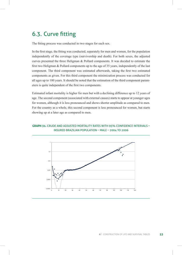
6.3. Curve fittingThefittingprocesswasconductedintwostagesforeachsex.
Inthefirststage,thefittingwasconducted,separatelyformenandwomen,forthepopulationindependently of the coverage type (survivorship and death). For both sexes, the adjusted curves presented the three Heligman & Pollard components. It was decided to estimate the firsttwoHeligman&Pollardcomponentsuptotheageof35years,independentlyofthelastcomponent.The thirdcomponentwasestimatedafterwards, taking thefirst twoestimatedcomponents as given. For this third component the minimization process was conducted for all ages up to 100 years. It should be noted that the estimation of the third component param-etersisquiteindependentofthefirsttwocomponents.
Estimated infant mortality is higher for men but with a declining difference up to 12 years of age. The second component (associated with external causes) starts to appear at younger ages for women, although it is less pronounced and shows shorter amplitude as compared to men. For the country as a whole, this second component is less pronounced for women, but starts showing up at a later age as compared to men.
grAPH 31. crUde and adJUSted MortalitY rateS With 95% conFidence intervalS – inSUred Brazilian PoPUlation – Male – 2004 to 2006
0,00001
0,0001
0,001
0,01
0,1
1
0 10 20 30 40 50 60 70 80 90 100 110 120
CRUDE AND ADJUSTED MORTALITY RATES WITH 95% CONFIDENCE INTERVALS – INSURED BRAZILIAN POPULATION – MALE – 2004 TO 2006
54BraZILIan mOrtaLItY anD surVIVOrsHIp LIFe taBLes
Insurance market experience – 2010
grAPH 32. crUde and adJUSted MortalitY rateS With 95% conFidence intervalS – inSUred Brazilian PoPUlation – FeMale – 2004 to 2006
0,00001
0,0001
0,001
0,01
0,1
1
0 10 20 30 40 50 60 70 80 90 100 110 120
CRUDE AND ADJUSTED MORTALITY RATES WITH 95% CONFIDENCE INTERVALS – INSURED BRAZILIAN POPULATION – FEMALE – 2004 TO 2006
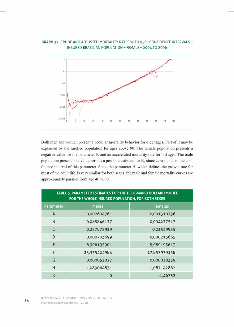
Both men and women present a peculiar mortality behavior for older ages. Part of it may be explainedby the rarefiedpopulationforagesabove90.Thefemalepopulationpresentsanegative value for the parameter K and an accelerated mortality rate for old ages. The male population presents the value zero as a possible estimate for K, since zero stands in the con-fidenceintervalofthisparameter.SincetheparameterH,whichdefinesthegrowthrateformost of the adult life, is very similar for both sexes, the male and female mortality curves are approximately parallel from age 40 to 90.
TABLe 5. PArAMeTer esTIMATes for THe HeLIgMAn & PoLLArD MoDeLfor THe wHoLe InsureD PoPuLATIon, for BoTH sexes
Parameter Males Females
a 0,002604761 0,001310736
B 0,085846127 0,094227517
c 0,257875929 0,22549935
d 0,000703699 0,000213665
e 6,996195901 5,989195613
F 23,335424984 17,857979158
G 0,000052027 0,000028359
h 1,089064831 1,087142882
k 0 -1,46752
556 cOnstructIOn OF LIFe anD surVIVaL taBLes
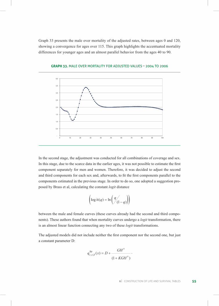
Graph 33 presents the male over mortality of the adjusted rates, between ages 0 and 120, showing a convergence for ages over 115. This graph highlights the accentuated mortality differences for younger ages and an almost parallel behavior from the ages 40 to 90.
grAPH 33. Male over MortalitY For adJUSted valUeS – 2004 to 2006
-
0,5
1,0
1,5
2,0
2,5
3,0
3,5
4,0
0 10 20 30 40 50 60 70 80 90 100
MALE OVER MORTALITY FOR ADJUSTED VALUES – 2004 TO 2006
In the second stage, the adjustment was conducted for all combinations of coverage and sex. Inthisstage,duetothescarcedataintheearlierages,itwasnotpossibletoestimatethefirstcomponent separately for men and women. Therefore, it was decided to adjust the second andthirdcomponentsforeachsexand,afterwards,tofitthefirstcomponentsparalleltothecomponents estimated in the previous stage. In order to do so, one adopted a suggestion pro-posed by Brass et al, calculating the constant logit distance
log ( ) ln ( )it q qq=
−( )( )1
between the male and female curves (these curves already had the second and third compo-nents). These authors found that when mortality curves undergo a logit transformation, there is an almost linear function connecting any two of these logit transformations.
Theadjustedmodelsdidnotincludeneitherthefirstcomponentnorthesecondone,butjusta constant parameter D:
q x DGH
KGHc s khp
x
x, , ( )( )
= ++1
.
56BraZILIan mOrtaLItY anD surVIVOrsHIp LIFe taBLes
Insurance market experience – 2010
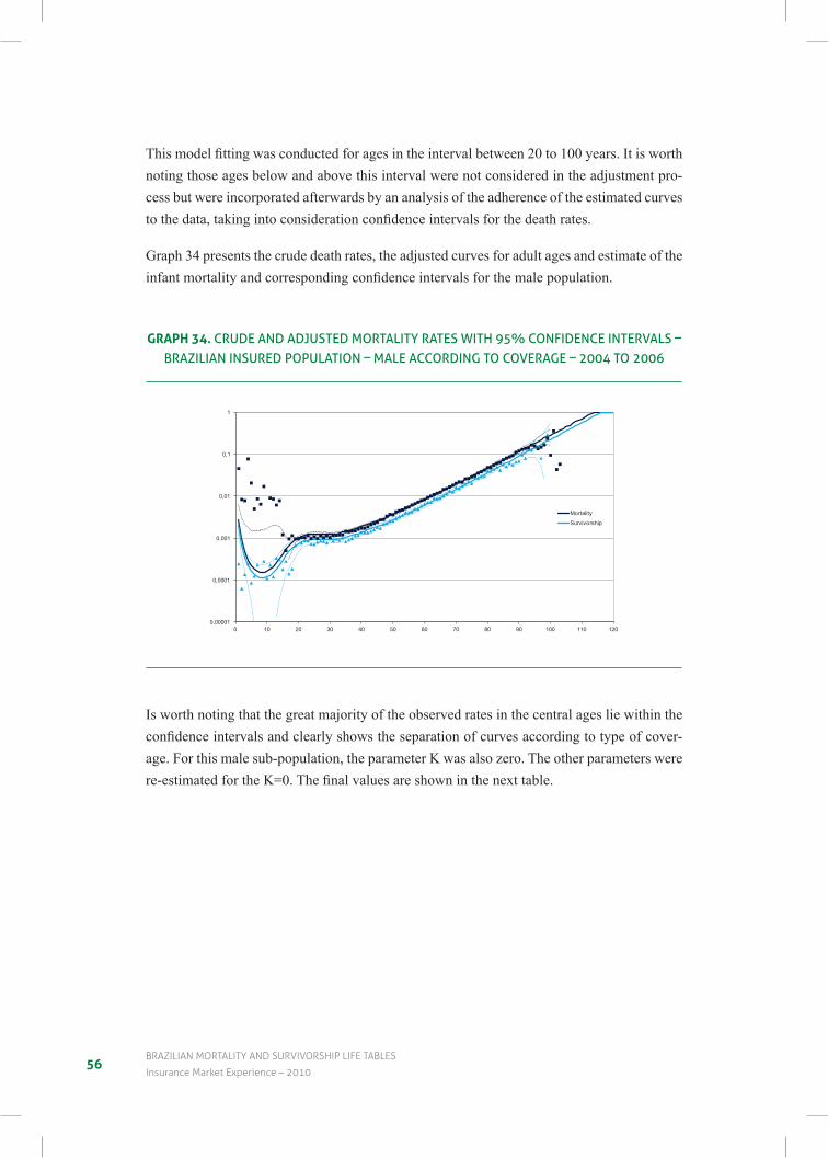
Thismodelfittingwasconductedforagesintheintervalbetween20to100years.Itisworthnoting those ages below and above this interval were not considered in the adjustment pro-cess but were incorporated afterwards by an analysis of the adherence of the estimated curves tothedata,takingintoconsiderationconfidenceintervalsforthedeathrates.
Graph 34 presents the crude death rates, the adjusted curves for adult ages and estimate of the infantmortalityandcorrespondingconfidenceintervalsforthemalepopulation.
grAPH 34. crUde and adJUSted MortalitY rateS With 95% conFidence intervalS – Brazilian inSUred PoPUlation – Male accordinG to coveraGe – 2004 to 2006
0,00001
0,0001
0,001
0,01
0,1
1
0 10 20 30 40 50 60 70 80 90 100 110 120
CRUDE AND ADJUSTED MORTALITY RATES WITH 95% CONFIDENCE INTERVALS – BRAZILIAN INSURED POPULATION – MALE ACCORDING TO COVERAGE – 2004 TO 2006
Mortality
Survivorship
Is worth noting that the great majority of the observed rates in the central ages lie within the confidenceintervalsandclearlyshowstheseparationofcurvesaccordingtotypeofcover-age. For this male sub-population, the parameter K was also zero. The other parameters were re-estimatedfortheK=0.Thefinalvaluesareshowninthenexttable.
576 cOnstructIOn OF LIFe anD surVIVaL taBLes
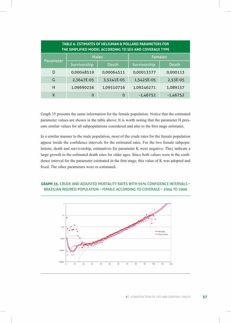
TABLe 6. esTIMATes of HeLIgMAn & PoLLArD PArAMeTers for THe sIMPLIfIeD MoDeL ACCorDIng To sex AnD CoverAge TyPe
ParameterMales Females
Survivorship death Survivorship death
d 0,00048519 0,00064511 0,00013377 0,000113
G 2,3647e-05 3,5241e-05 1,5425e-05 2,53e-05
h 1,09690236 1,09510716 1,09246271 1,089157
k 0 0 -1,46752 -1,46752
Graph 35 presents the same information for the female population. Notice that the estimated parameter values are shown in the table above. It is worth noting that the parameter H pres-entssimilarvaluesforallsubpopulationsconsideredandalsotothefirststageestimates.
In a similar manner to the male population, most of the crude rates for the female population appearinsidetheconfidenceintervalsfortheestimatedrates.Forthetwofemalesubpopu-lations, death and survivorship, estimatives for parameter K were negative. They indicate a largegrowthintheestimateddeathratesforolderages.Sincebothvalueswereintheconfi-denceintervalfortheparameterestimatedinthefirststage,thisvalueofKwasadoptedandfixed.Theotherparameterswerere-estimated.
grAPH 35. crUde and adJUSted MortalitY rateS With 95% conFidence intervalS – Brazilian inSUred PoPUlation – FeMale accordinG to coveraGe – 2004 to 2006
0,00001
0,0001
0,001
0,01
0,1
1
0 10 20 30 40 50 60 70 80 90 100 110 120
CRUDE AND ADJUSTED MORTALITY RATES WITH 95% CONFIDENCE INTERVALS – BRAZILIAN INSURED POPULATION – FEMALE ACCORDING TO COVERAGE – 2004 TO 2006
Mortality
Survivorship
58BraZILIan mOrtaLItY anD surVIVOrsHIp LIFe taBLes
Insurance market experience – 2010
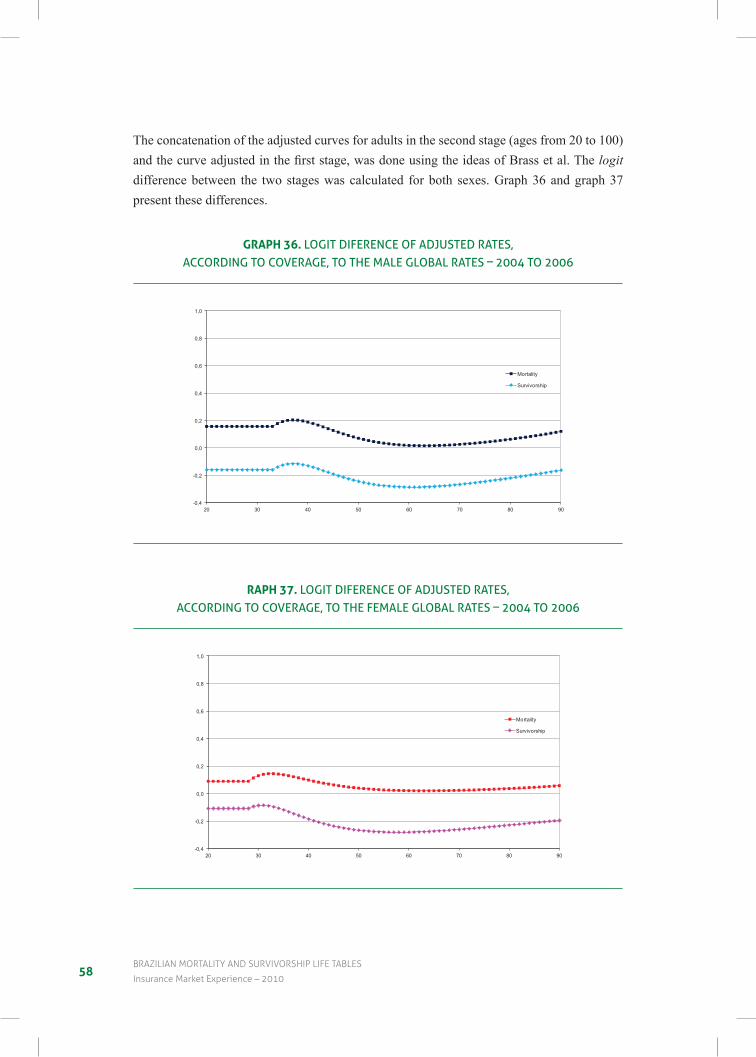
The concatenation of the adjusted curves for adults in the second stage (ages from 20 to 100) andthecurveadjustedinthefirststage,wasdoneusingtheideasofBrassetal.Thelogit difference between the two stages was calculated for both sexes. Graph 36 and graph 37 present these differences.
grAPH 36. loGit diFerence oF adJUSted rateS, accordinG to coveraGe, to the Male GloBal rateS – 2004 to 2006
-0,4
-0,2
0,0
0,2
0,4
0,6
0,8
1,0
20 30 40 50 60 70 80 90
LOGIT DIFFERENCE OF ADJUSTED RATES, ACCORDING TO COVERAGE, TO THE MALE GLOBAL RATES – 2004 TO 2006
Mortality
Survivorship
rAPH 37. loGit diFerence oF adJUSted rateS, accordinG to coveraGe, to the FeMale GloBal rateS – 2004 to 2006
-0,4
-0,2
0,0
0,2
0,4
0,6
0,8
1,0
20 30 40 50 60 70 80 90
LOGIT DIFFERENCE OF ADJUSTED RATES, ACCORDING TO COVERAGE, TO THE FEMALE GLOBAL RATES – 2004 TO 2006
Mortality
Survivorship
596 cOnstructIOn OF LIFe anD surVIVaL taBLes
One sees that these differences are reasonably constant from 20 to 90 years of age for both sexes. Therefore, it can be assumed that this difference can be extended for ages below 20, sinceinthefirststagethemortalitycurvesforchildrenwereestimatedforallindividualsindependently of coverage types. Hence the mortality rates for the beginning of the curve were established through the use of the following equation:
log ( ) log ( ), ,ito itoq x q xc shp
shp
c s( ) ( )= +α
where
q xc shp, ( ) is the adjusted mortality rate for those with coverage c and sex s for ages x in the
interval from 0 to 20;
q xshp ( ) is the adjusted mortality rate for those with sex s and age x in the interval from 0
to20,estimatedinthefirststage;
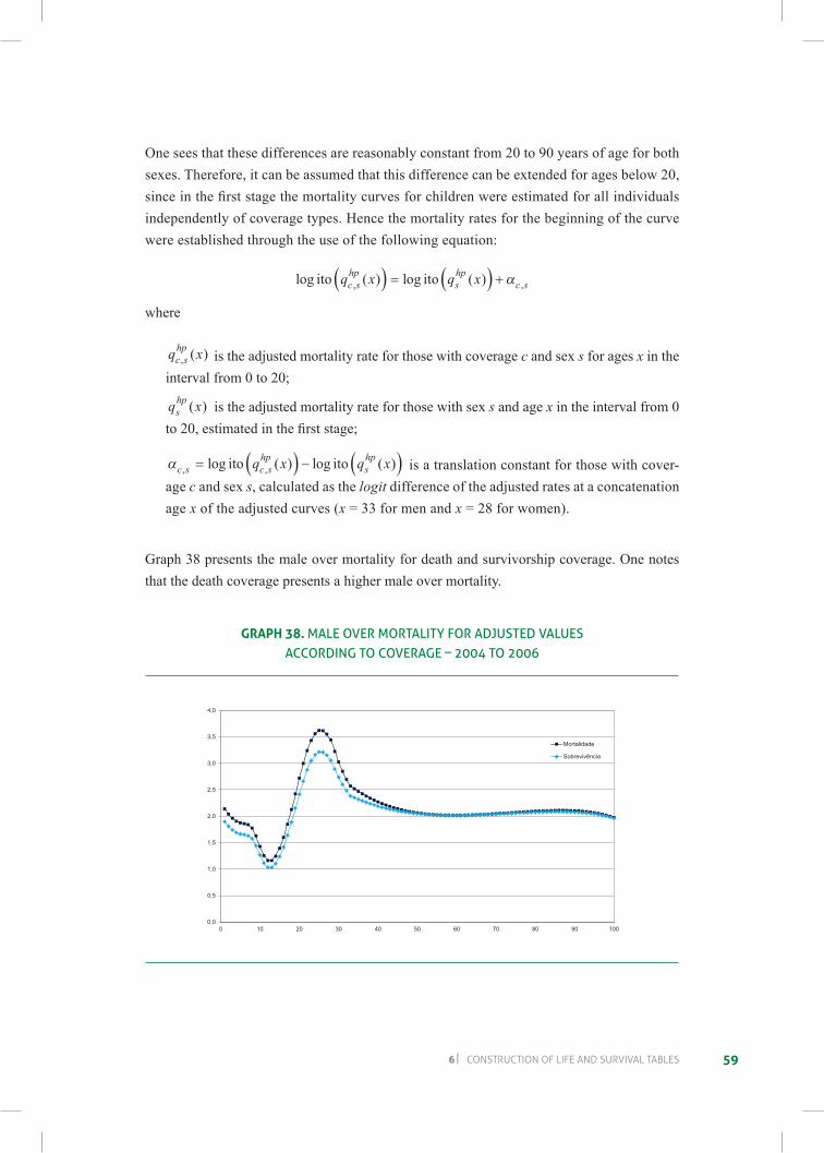
αc s c shp
shpq x q x, ,log ( ) log ( )= −( ) ( )ito ito is a translation constant for those with cover-
age c and sex s, calculated as the logit difference of the adjusted rates at a concatenation age x of the adjusted curves (x = 33 for men and x = 28 for women).
Graph 38 presents the male over mortality for death and survivorship coverage. One notes that the death coverage presents a higher male over mortality.
grAPH 38. Male over MortalitY For adJUSted valUeSaccordinG to coveraGe – 2004 to 2006
0,0
0,5
1,0
1,5
2,0
2,5
3,0
3,5
4,0
0 10 20 30 40 50 60 70 80 90 100
SOBREMORTALIDADE MASCULINA DOS VALORES AJUSTADOS SEGUNDO COBERTURA – 2004 A 2006
Mortalidade
Sobrevivência
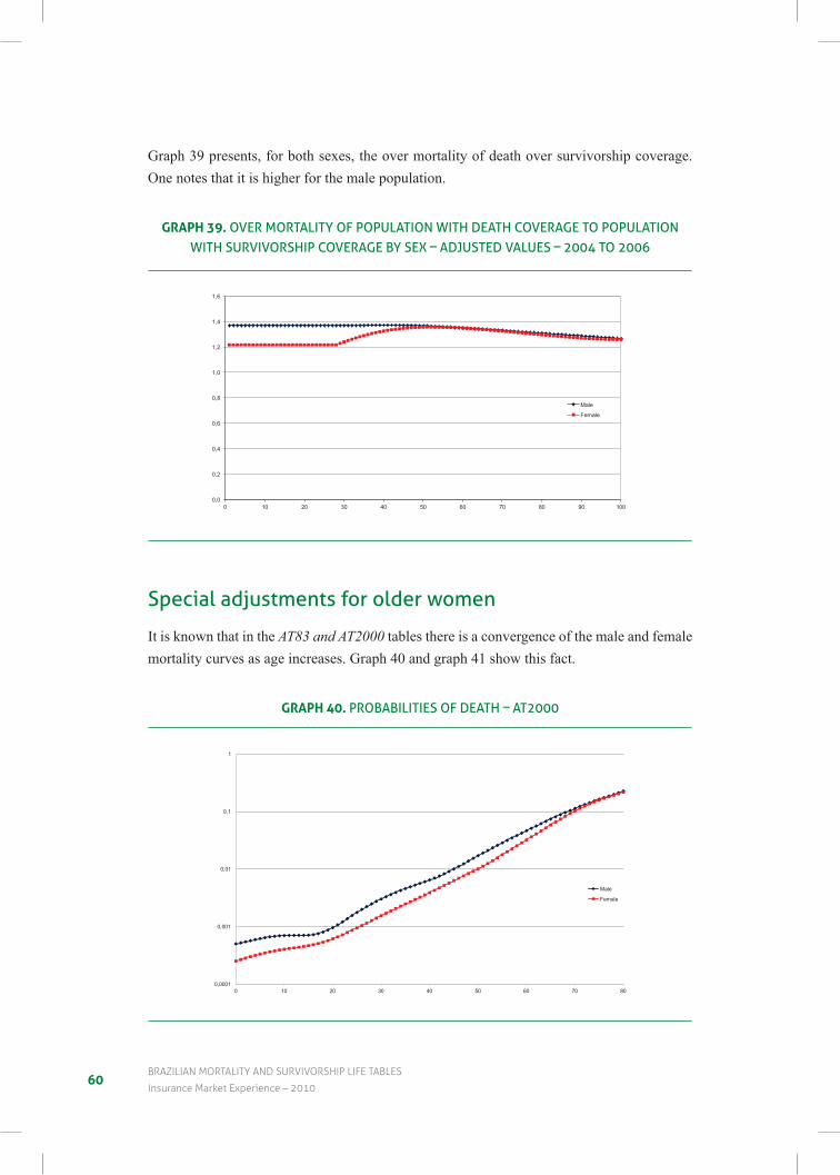
60BraZILIan mOrtaLItY anD surVIVOrsHIp LIFe taBLes
Insurance market experience – 2010
Graph 39 presents, for both sexes, the over mortality of death over survivorship coverage. One notes that it is higher for the male population.
grAPH 39. over MortalitY oF PoPUlation With death coveraGe to PoPUlation With SUrvivorShiP coveraGe BY SeX – adJUSted valUeS – 2004 to 2006
0,0
0,2
0,4
0,6
0,8
1,0
1,2
1,4
1,6
0 10 20 30 40 50 60 70 80 90 100
OVER MORTALITY OF POPULATION WITH DEATH COVERAGE TO POPULATION WITH SURVIVORSHIP COVERAGE BY SEX – ADJUSTED
VALUES – 2004 TO 2006
Male
Female
Special adjustments for older women
It is known that in the AT83 and AT2000 tables there is a convergence of the male and female mortality curves as age increases. Graph 40 and graph 41 show this fact.
grAPH 40. ProBaBilitieS oF death – at2000
0,0001
0,001
0,01
0,1
1
0 10 20 30 40 50 60 70 80
PROBABILITIES OF DEATH – AT2000
Male
Female
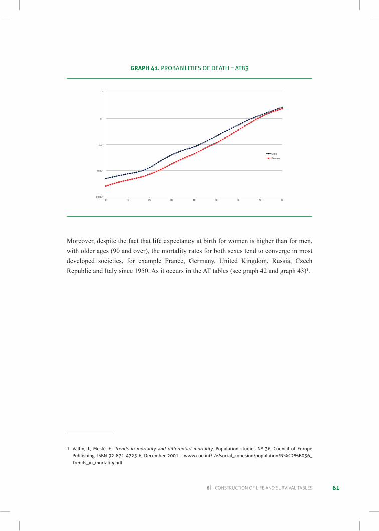
616 cOnstructIOn OF LIFe anD surVIVaL taBLes
grAPH 41. ProBaBilitieS oF death – at83
0,0001
0,001
0,01
0,1
1
0 10 20 30 40 50 60 70 80
PROBABILITIES OF DEATH – AT83
Male
Female
Moreover, despite the fact that life expectancy at birth for women is higher than for men, with older ages (90 and over), the mortality rates for both sexes tend to converge in most developed societies, for example France, Germany, United Kingdom, Russia, Czech Republic and Italy since 1950. As it occurs in the AT tables (see graph 42 and graph 43)1.
1 vallin, J., Meslé, F.; Trends in mortality and differential mortality, Population studies nº 36, council of europe Publishing, ISBN 92-871-4725-6, December 2001 – www.coe.int/t/e/social_cohesion/population/N%C2%B036_Trends_in_mortality.pdf
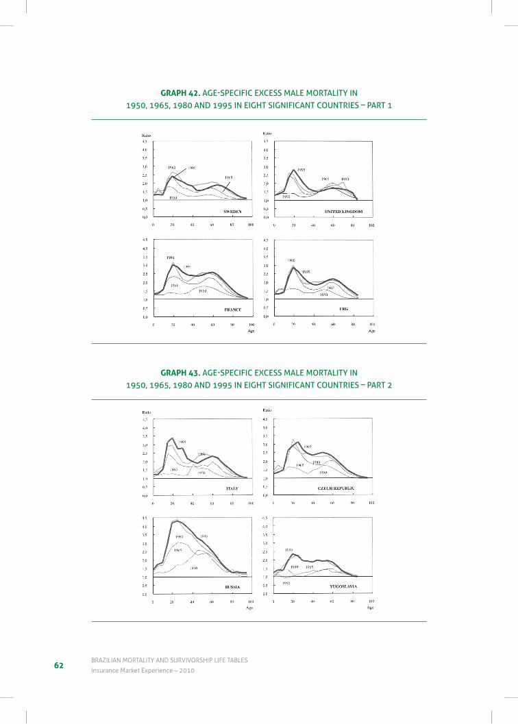
62BraZILIan mOrtaLItY anD surVIVOrsHIp LIFe taBLes
Insurance market experience – 2010
grAPH 42. AGE-SPECIFIC EXCESS MALE MORTALITY IN 1950, 1965, 1980 and 1995 in eiGht SiGniFicant coUntrieS – Part 1
grAPH 43. AGE-SPECIFIC EXCESS MALE MORTALITY IN 1950, 1965, 1980 and 1995 in eiGht SiGniFicant coUntrieS – Part 2
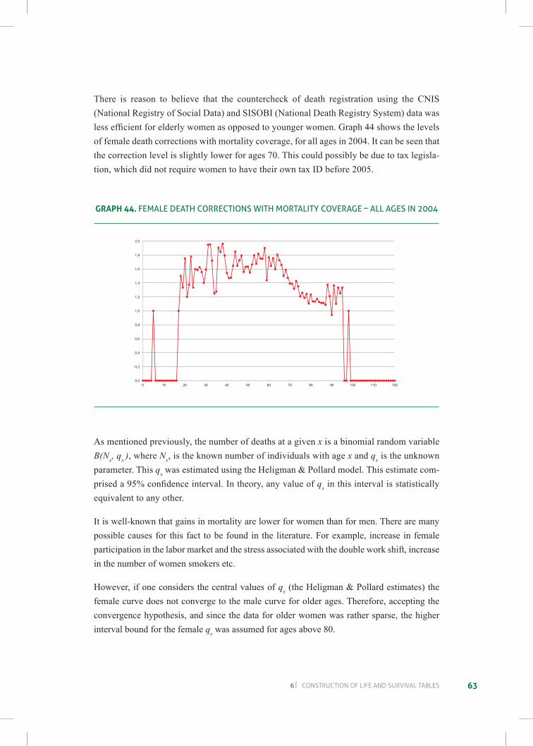
636 cOnstructIOn OF LIFe anD surVIVaL taBLes
There is reason to believe that the countercheck of death registration using the CNIS (National Registry of Social Data) and SISOBI (National Death Registry System) data was lessefficientforelderlywomenasopposedtoyoungerwomen.Graph44showsthelevelsof female death corrections with mortality coverage, for all ages in 2004. It can be seen that the correction level is slightly lower for ages 70. This could possibly be due to tax legisla-tion, which did not require women to have their own tax ID before 2005.
grAPH 44. FeMale death correctionS With MortalitY coveraGe – all aGeS in 2004
0,0
0,2
0,4
0,6
0,8
1,0
1,2
1,4
1,6
1,8
2,0
0 10 20 30 40 50 60 70 80 90 100 110 120
FEMALE DEATH CORRECTIONS WITH MORTALITY COVERAGE – ALL AGES IN 2004
As mentioned previously, the number of deaths at a given x is a binomial random variable B(Nx, qx ), where Nx, is the known number of individuals with age x and qx is the unknown parameter. This qx was estimated using the Heligman & Pollard model. This estimate com-priseda95%confidenceinterval.Intheory,anyvalueofqx in this interval is statistically equivalent to any other.
It is well-known that gains in mortality are lower for women than for men. There are many possible causes for this fact to be found in the literature. For example, increase in female participation in the labor market and the stress associated with the double work shift, increase in the number of women smokers etc.
However, if one considers the central values of qx (the Heligman & Pollard estimates) the female curve does not converge to the male curve for older ages. Therefore, accepting the convergence hypothesis, and since the data for older women was rather sparse, the higher interval bound for the female qx was assumed for ages above 80.
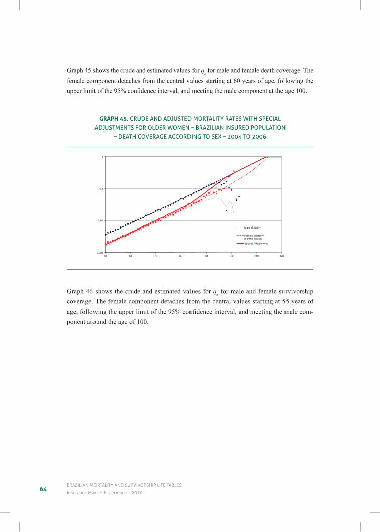
64BraZILIan mOrtaLItY anD surVIVOrsHIp LIFe taBLes
Insurance market experience – 2010
Graph 45 shows the crude and estimated values for qx for male and female death coverage. The female component detaches from the central values starting at 60 years of age, following the upperlimitofthe95%confidenceinterval,andmeetingthemalecomponentattheage100.
grAPH 45. crUde and adJUSted MortalitY rateS With SPecial adJUStMentS For older WoMen – Brazilian inSUred PoPUlation
– death coveraGe accordinG to SeX – 2004 to 2006
0,001
0,01
0,1
1
50 60 70 80 90 100 110 120
CRUDE AND ADJUSTED MORTALITY RATES WITH SPECIAL ADJUSTMENTS FOR OLDER WOMEN – BRAZILIAN INSURED POPULATION – DEATH COVERAGE ACCORDING TO SEX – 2004 TO 2006
Male Mortality
Female Mortality (central values)
Special Adjustments
Graph 46 shows the crude and estimated values for qx for male and female survivorship coverage. The female component detaches from the central values starting at 55 years of age,followingtheupperlimitofthe95%confidenceinterval,andmeetingthemalecom-ponent around the age of 100.
656 cOnstructIOn OF LIFe anD surVIVaL taBLes
grAPH 46. crUde and adJUSted MortalitY rateS With SPecial adJUStMentS For older WoMen – Brazilian inSUred PoPUlation
– SUrvivorShiP coveraGe accordinG to SeX – 2004 to 2006
0,001
0,01
0,1
1
50 60 70 80 90 100 110 120
CRUDE AND ADJUSTED MORTALITY RATES WITH SPECIAL ADJUSTMENTS FOR OLDER WOMEN – BRAZILIAN INSURED POPULATION – SURVIVORSHIP COVERAGE ACCORDING TO SEX – 2004
TO 2006
Male Survivorship
Female Survivorship (central values)
Special Adjustments
Graph 47 shows the crude and estimated values for qx for men and women and for both cover-age types. Note that each dot corresponds to a given crude rate. These crude rates were calcu-lated based on different numbers of insureds. In particular, for older ages, it’s usual for these numberstoberathersmall.Asaconsequence,confidenceintervalstendtobeverylarge.
grAPH 47. crUde and adJUSted MortalitY rateS accordinG to SeX and coveraGeS With SPecial adJUStMentS For older WoMen – 2004 to 2006
0,00001
0,0001
0,001
0,01
0,1
1
0 10 20 30 40 50 60 70 80 90 100 110 120
CRUDE AND ADJUSTED MORTALITY RATES ACCORDING TO SEX AND COVERAGES WITH SPECIAL ADJUSTMENTS FOR OLDER WOMEN – 2004 TO 2006
Male Mortality: BR-EMSmt – v.2010 -m
Male Survivorship: BR-EMSsb – v.2010 -m
Female Mortality: BR-EMSmt – v.2010 -f
Female survivorship: BR-EMSsb – v.2010 -f


67
7 Br-eMs Tables
t he adjusted life table, denominated “Experiência do Mercado Segurador Brasileiro – BR-EMS”,presentsvariantsclassifiedaccording tocoverage typeandsex.Thegiven names of these variants follow the usual life table nomenclature, coverage type
– “sb” for survivorship and “mt” for mortality – and sex.
Although the life tables relate to the death experience for the years 2004 to 2006, centered on2005,theywereofficiallyadoptedasstandardtablesbySUSEPasthe2010versionoftheBR-EMS, due to the year of its publication (SUSEP Circular nº 402, 18.03.2010 – D.O.U.: 19.03.2010).
Hence, we have the following variants of the BR-EMS.
• BR-EMSsb-v.2010-m
• BR-EMSsb-v.2010-f
• BR-EMSmt-v.2010-m
• BR-EMSmt-v.2010-f
Each variant comprises the following parameters:
• qx – probability (or rate) of death between ages x and x+1;
• lx – number of living at age x;
• ex – life expectancy at age x;
• +IC(95%)–upperboundof95%confidenceintervaland
• -IC(95%)–lowerboundof95%confidenceinterval.
Confidenceintervalswereobtainedusingthenormalapproximationtothebinomialdistribu-tion. Hence negative values are not to be considered.
68BraZILIan mOrtaLItY anD surVIVOrsHIp LIFe taBLes
Insurance market experience – 2010
7.1 Male survivorship: Br-eMSsb-v.2010-mTable 7 presents the “BR-EMSsb-v.2010-m” life table for males with survivorship coverage type,fromages0to116.Extremevaluesofthe95%confidenceintervals(IC)aregiveninred for the younger ages and in black otherwise.
TAble 7. MAle SurvivorShip: br-eMSsb-v.2010-m
age qx -ic (95%) +ic (95%) lx ex
0 0,00200 0,00090 0,00210 1.000.000 81,9
1 0,00069 0,00030 0,00080 997.997 81,0
2 0,00035 0,00020 0,00060 997.308 80,1
3 0,00022 0,00010 0,00050 996.957 79,1
4 0,00016 0,00010 0,00050 996.735 78,1
5 0,00013 0,00010 0,00050 996.573 77,1
6 0,00012 0,00010 0,00040 996.440 76,1
7 0,00011 0,00010 0,00040 996.322 75,2
8 0,00011 0,00010 0,00040 996.210 74,2
9 0,00012 0,00010 0,00050 996.098 73,2
10 0,00013 0,00010 0,00050 995.981 72,2
11 0,00015 0,00010 0,00050 995.853 71,2
12 0,00019 0,00010 0,00060 995.702 70,2
13 0,00024 0,00020 0,00070 995.516 69,2
14 0,00031 0,00020 0,00080 995.279 68,2
15 0,00039 0,00020 0,00080 994.975 67,3
16 0,00048 0,00030 0,00090 994.591 66,3
17 0,00057 0,00030 0,00090 994.118 65,3
18 0,00066 0,00040 0,00090 993.554 64,3
19 0,00074 0,00040 0,00090 992.902 63,4
20 0,00080 0,00050 0,00090 992.171 62,4
21 0,00085 0,00050 0,00090 991.375 61,5
22 0,00089 0,00050 0,00080 990.527 60,5
23 0,00092 0,00050 0,00080 989.644 59,6
24 0,00093 0,00050 0,00080 988.738 58,6
697 BR-EMS TaBlES
TAble 7. MAle SurvivorShip: br-eMSsb-v.2010-m
age qx -ic (95%) +ic (95%) lx ex
25 0,00093 0,00050 0,00080 987.822 57,7
26 0,00093 0,00050 0,00080 986.903 56,7
27 0,00092 0,00060 0,00080 985.988 55,8
28 0,00092 0,00060 0,00080 985.079 54,9
29 0,00091 0,00060 0,00090 984.176 53,9
30 0,00092 0,00060 0,00090 983.275 53,0
31 0,00093 0,00070 0,00090 982.374 52,0
32 0,00094 0,00070 0,00100 981.465 51,0
33 0,00099 0,00070 0,00100 980.541 50,1
34 0,00103 0,00080 0,00100 979.574 49,1
35 0,00109 0,00080 0,00110 978.561 48,2
36 0,00115 0,00080 0,00110 977.497 47,2
37 0,00121 0,00090 0,00120 976.377 46,3
38 0,00128 0,00090 0,00120 975.196 45,4
39 0,00136 0,00100 0,00130 973.948 44,4
40 0,00144 0,00110 0,00140 972.627 43,5
41 0,00153 0,00110 0,00140 971.225 42,5
42 0,00164 0,00120 0,00150 969.735 41,6
43 0,00175 0,00130 0,00160 968.149 40,7
44 0,00187 0,00140 0,00170 966.458 39,7
45 0,00200 0,00150 0,00190 964.651 38,8
46 0,00215 0,00160 0,00200 962.719 37,9
47 0,00231 0,00170 0,00220 960.648 37,0
48 0,00249 0,00190 0,00230 958.427 36,1
49 0,00268 0,00200 0,00250 956.042 35,1
50 0,00290 0,00220 0,00270 953.477 34,2
51 0,00313 0,00240 0,00300 950.715 33,3
52 0,00339 0,00260 0,00320 947.740 32,4
53 0,00367 0,00280 0,00350 944.531 31,5
54 0,00398 0,00310 0,00380 941.067 30,7
55 0,00431 0,00340 0,00420 937.326 29,8
70BraZILIan mOrtaLItY anD surVIVOrsHIp LIFe taBLes
Insurance market experience – 2010
TAble 7. MAle SurvivorShip: br-eMSsb-v.2010-m
age qx -ic (95%) +ic (95%) lx ex
56 0,00468 0,00370 0,00460 933.283 28,9
57 0,00509 0,00400 0,00500 928.911 28,0
58 0,00554 0,00440 0,00550 924.182 27,2
59 0,00603 0,00480 0,00600 919.064 26,3
60 0,00656 0,00530 0,00660 913.524 25,5
61 0,00715 0,00580 0,00730 907.527 24,6
62 0,00780 0,00640 0,00800 901.035 23,8
63 0,00851 0,00700 0,00880 894.007 23,0
64 0,00929 0,00760 0,00970 886.400 22,2
65 0,01014 0,00840 0,01060 878.169 21,4
66 0,01107 0,00920 0,01160 869.266 20,6
67 0,01210 0,01010 0,01280 859.639 19,8
68 0,01323 0,01110 0,01400 849.237 19,1
69 0,01446 0,01220 0,01530 838.005 18,3
70 0,01581 0,01340 0,01680 825.887 17,6
71 0,01730 0,01460 0,01850 812.826 16,9
72 0,01893 0,01590 0,02030 798.763 16,2
73 0,02072 0,01740 0,02220 783.643 15,5
74 0,02268 0,01910 0,02420 767.408 14,8
75 0,02483 0,02080 0,02650 750.005 14,1
76 0,02719 0,02260 0,02890 731.384 13,4
77 0,02977 0,02460 0,03150 711.500 12,8
78 0,03261 0,02670 0,03430 690.315 12,2
79 0,03573 0,02890 0,03730 667.802 11,6
80 0,03914 0,03110 0,04060 643.944 11,0
81 0,04289 0,03330 0,04430 618.740 10,4
82 0,04700 0,03530 0,04840 592.204 9,9
83 0,05150 0,03750 0,05270 564.373 9,3
84 0,05645 0,03970 0,05720 535.306 8,8
85 0,06187 0,04180 0,06200 505.090 8,3
86 0,06782 0,04380 0,06730 473.841 7,8
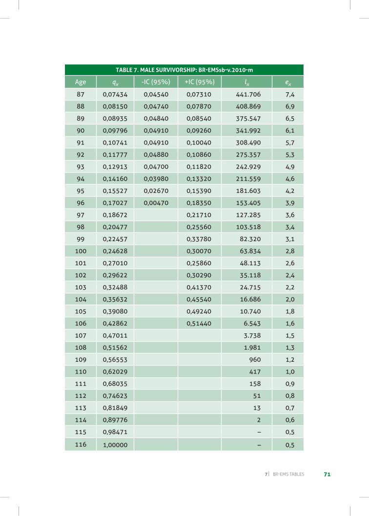
717 BR-EMS TaBlES
TAble 7. MAle SurvivorShip: br-eMSsb-v.2010-m
age qx -ic (95%) +ic (95%) lx ex
87 0,07434 0,04540 0,07310 441.706 7,4
88 0,08150 0,04740 0,07870 408.869 6,9
89 0,08935 0,04840 0,08540 375.547 6,5
90 0,09796 0,04910 0,09260 341.992 6,1
91 0,10741 0,04910 0,10040 308.490 5,7
92 0,11777 0,04880 0,10860 275.357 5,3
93 0,12913 0,04700 0,11820 242.929 4,9
94 0,14160 0,03980 0,13320 211.559 4,6
95 0,15527 0,02670 0,15390 181.603 4,2
96 0,17027 0,00470 0,18350 153.405 3,9
97 0,18672 0,21710 127.285 3,6
98 0,20477 0,25560 103.518 3,4
99 0,22457 0,33780 82.320 3,1
100 0,24628 0,30070 63.834 2,8
101 0,27010 0,25860 48.113 2,6
102 0,29622 0,30290 35.118 2,4
103 0,32488 0,41370 24.715 2,2
104 0,35632 0,45540 16.686 2,0
105 0,39080 0,49240 10.740 1,8
106 0,42862 0,51440 6.543 1,6
107 0,47011 3.738 1,5
108 0,51562 1.981 1,3
109 0,56553 960 1,2
110 0,62029 417 1,0
111 0,68035 158 0,9
112 0,74623 51 0,8
113 0,81849 13 0,7
114 0,89776 2 0,6
115 0,98471 – 0,5
116 1,00000 – 0,5
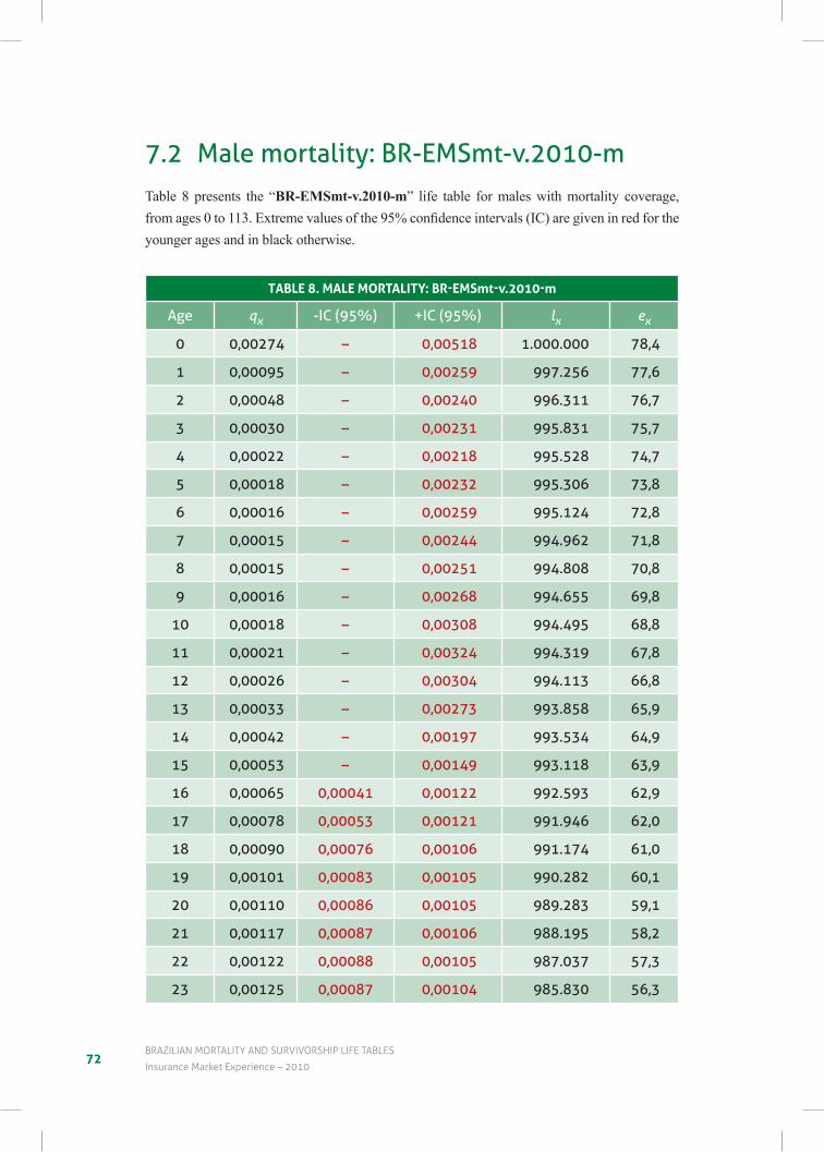
72BraZILIan mOrtaLItY anD surVIVOrsHIp LIFe taBLes
Insurance market experience – 2010
7.2 Male mortality: Br-eMSmt-v.2010-mTable 8 presents the “BR-EMSmt-v.2010-m” life table for males with mortality coverage, fromages0to113.Extremevaluesofthe95%confidenceintervals(IC)aregiveninredfortheyounger ages and in black otherwise.
TAble 8. MAle MorTAliTy: br-eMSmt-v.2010-m
age qx -ic (95%) +ic (95%) lx ex
0 0,00274 – 0,00518 1.000.000 78,4
1 0,00095 – 0,00259 997.256 77,6
2 0,00048 – 0,00240 996.311 76,7
3 0,00030 – 0,00231 995.831 75,7
4 0,00022 – 0,00218 995.528 74,7
5 0,00018 – 0,00232 995.306 73,8
6 0,00016 – 0,00259 995.124 72,8
7 0,00015 – 0,00244 994.962 71,8
8 0,00015 – 0,00251 994.808 70,8
9 0,00016 – 0,00268 994.655 69,8
10 0,00018 – 0,00308 994.495 68,8
11 0,00021 – 0,00324 994.319 67,8
12 0,00026 – 0,00304 994.113 66,8
13 0,00033 – 0,00273 993.858 65,9
14 0,00042 – 0,00197 993.534 64,9
15 0,00053 – 0,00149 993.118 63,9
16 0,00065 0,00041 0,00122 992.593 62,9
17 0,00078 0,00053 0,00121 991.946 62,0
18 0,00090 0,00076 0,00106 991.174 61,0
19 0,00101 0,00083 0,00105 990.282 60,1
20 0,00110 0,00086 0,00105 989.283 59,1
21 0,00117 0,00087 0,00106 988.195 58,2
22 0,00122 0,00088 0,00105 987.037 57,3
23 0,00125 0,00087 0,00104 985.830 56,3
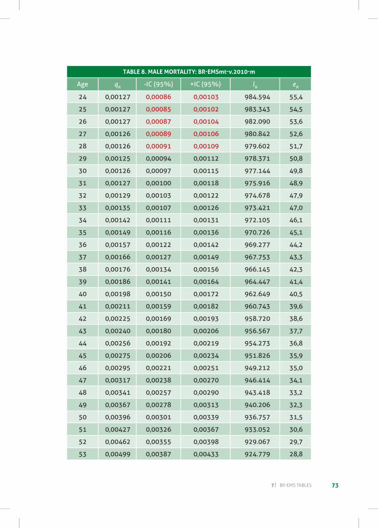
737 BR-EMS TaBlES
TAble 8. MAle MorTAliTy: br-eMSmt-v.2010-m
age qx -ic (95%) +ic (95%) lx ex
24 0,00127 0,00086 0,00103 984.594 55,4
25 0,00127 0,00085 0,00102 983.343 54,5
26 0,00127 0,00087 0,00104 982.090 53,6
27 0,00126 0,00089 0,00106 980.842 52,6
28 0,00126 0,00091 0,00109 979.602 51,7
29 0,00125 0,00094 0,00112 978.371 50,8
30 0,00126 0,00097 0,00115 977.144 49,8
31 0,00127 0,00100 0,00118 975.916 48,9
32 0,00129 0,00103 0,00122 974.678 47,9
33 0,00135 0,00107 0,00126 973.421 47,0
34 0,00142 0,00111 0,00131 972.105 46,1
35 0,00149 0,00116 0,00136 970.726 45,1
36 0,00157 0,00122 0,00142 969.277 44,2
37 0,00166 0,00127 0,00149 967.753 43,3
38 0,00176 0,00134 0,00156 966.145 42,3
39 0,00186 0,00141 0,00164 964.447 41,4
40 0,00198 0,00150 0,00172 962.649 40,5
41 0,00211 0,00159 0,00182 960.743 39,6
42 0,00225 0,00169 0,00193 958.720 38,6
43 0,00240 0,00180 0,00206 956.567 37,7
44 0,00256 0,00192 0,00219 954.273 36,8
45 0,00275 0,00206 0,00234 951.826 35,9
46 0,00295 0,00221 0,00251 949.212 35,0
47 0,00317 0,00238 0,00270 946.414 34,1
48 0,00341 0,00257 0,00290 943.418 33,2
49 0,00367 0,00278 0,00313 940.206 32,3
50 0,00396 0,00301 0,00339 936.757 31,5
51 0,00427 0,00326 0,00367 933.052 30,6
52 0,00462 0,00355 0,00398 929.067 29,7
53 0,00499 0,00387 0,00433 924.779 28,8
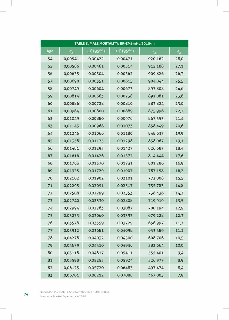
74BraZILIan mOrtaLItY anD surVIVOrsHIp LIFe taBLes
Insurance market experience – 2010
TAble 8. MAle MorTAliTy: br-eMSmt-v.2010-m
age qx -ic (95%) +ic (95%) lx ex
54 0,00541 0,00422 0,00471 920.162 28,0
55 0,00586 0,00461 0,00514 915.188 27,1
56 0,00635 0,00504 0,00562 909.826 26,3
57 0,00690 0,00551 0,00615 904.044 25,5
58 0,00749 0,00604 0,00673 897.808 24,6
59 0,00814 0,00663 0,00738 891.081 23,8
60 0,00886 0,00728 0,00810 883.824 23,0
61 0,00964 0,00800 0,00889 875.996 22,2
62 0,01049 0,00880 0,00976 867.553 21,4
63 0,01143 0,00968 0,01073 858.449 20,6
64 0,01246 0,01066 0,01180 848.637 19,9
65 0,01358 0,01175 0,01298 838.067 19,1
66 0,01481 0,01295 0,01427 826.687 18,4
67 0,01616 0,01426 0,01572 814.444 17,6
68 0,01763 0,01570 0,01731 801.286 16,9
69 0,01925 0,01729 0,01907 787.158 16,2
70 0,02102 0,01902 0,02101 772.008 15,5
71 0,02295 0,02091 0,02317 755.783 14,8
72 0,02508 0,02299 0,02553 738.436 14,2
73 0,02740 0,02530 0,02808 719.919 13,5
74 0,02994 0,02783 0,03087 700.194 12,9
75 0,03273 0,03060 0,03393 679.228 12,3
76 0,03578 0,03359 0,03729 656.997 11,7
77 0,03912 0,03681 0,04098 633.489 11,1
78 0,04278 0,04032 0,04500 608.706 10,5
79 0,04679 0,04410 0,04936 582.664 10,0
80 0,05118 0,04817 0,05411 555.401 9,4
81 0,05598 0,05255 0,05924 526.977 8,9
82 0,06125 0,05720 0,06483 497.474 8,4
83 0,06701 0,06212 0,07088 467.005 7,9
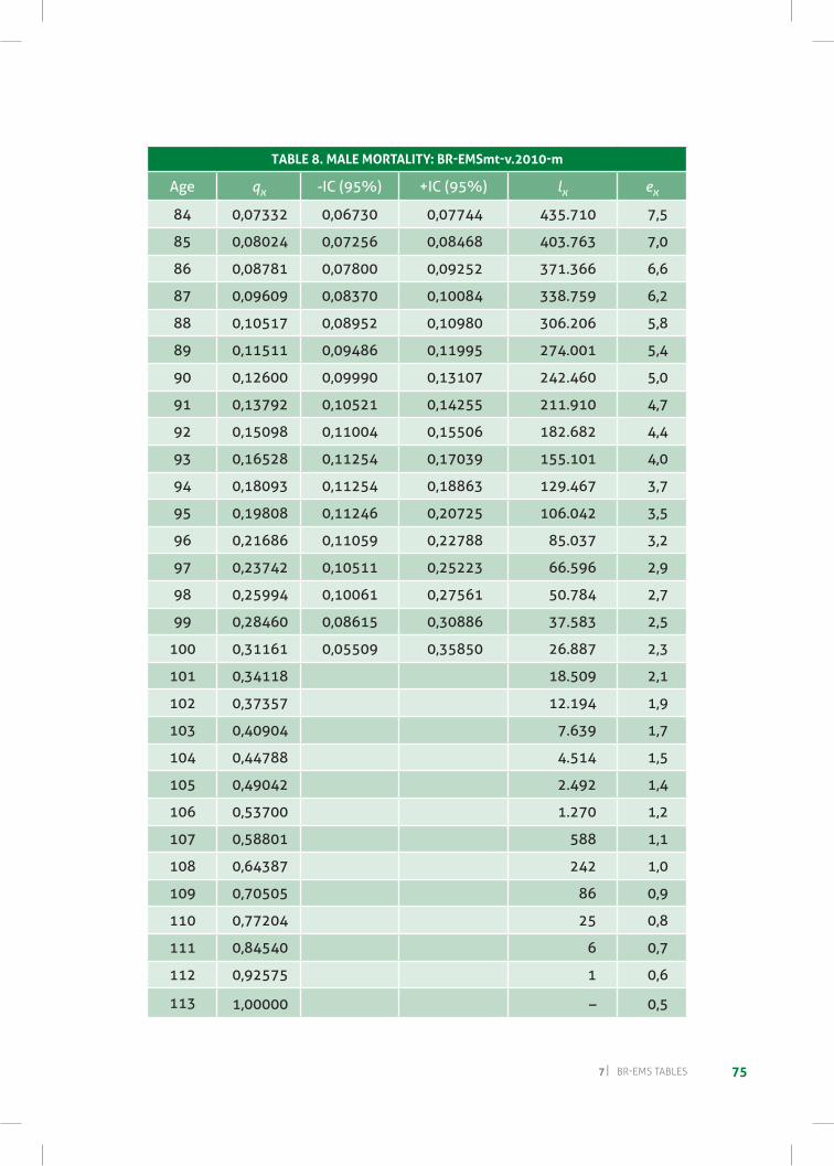
757 BR-EMS TaBlES
TAble 8. MAle MorTAliTy: br-eMSmt-v.2010-m
age qx -ic (95%) +ic (95%) lx ex
84 0,07332 0,06730 0,07744 435.710 7,5
85 0,08024 0,07256 0,08468 403.763 7,0
86 0,08781 0,07800 0,09252 371.366 6,6
87 0,09609 0,08370 0,10084 338.759 6,2
88 0,10517 0,08952 0,10980 306.206 5,8
89 0,11511 0,09486 0,11995 274.001 5,4
90 0,12600 0,09990 0,13107 242.460 5,0
91 0,13792 0,10521 0,14255 211.910 4,7
92 0,15098 0,11004 0,15506 182.682 4,4
93 0,16528 0,11254 0,17039 155.101 4,0
94 0,18093 0,11254 0,18863 129.467 3,7
95 0,19808 0,11246 0,20725 106.042 3,5
96 0,21686 0,11059 0,22788 85.037 3,2
97 0,23742 0,10511 0,25223 66.596 2,9
98 0,25994 0,10061 0,27561 50.784 2,7
99 0,28460 0,08615 0,30886 37.583 2,5
100 0,31161 0,05509 0,35850 26.887 2,3
101 0,34118 18.509 2,1
102 0,37357 12.194 1,9
103 0,40904 7.639 1,7
104 0,44788 4.514 1,5
105 0,49042 2.492 1,4
106 0,53700 1.270 1,2
107 0,58801 588 1,1
108 0,64387 242 1,0
109 0,70505 86 0,9
110 0,77204 25 0,8
111 0,84540 6 0,7
112 0,92575 1 0,6
113 1,00000 – 0,5
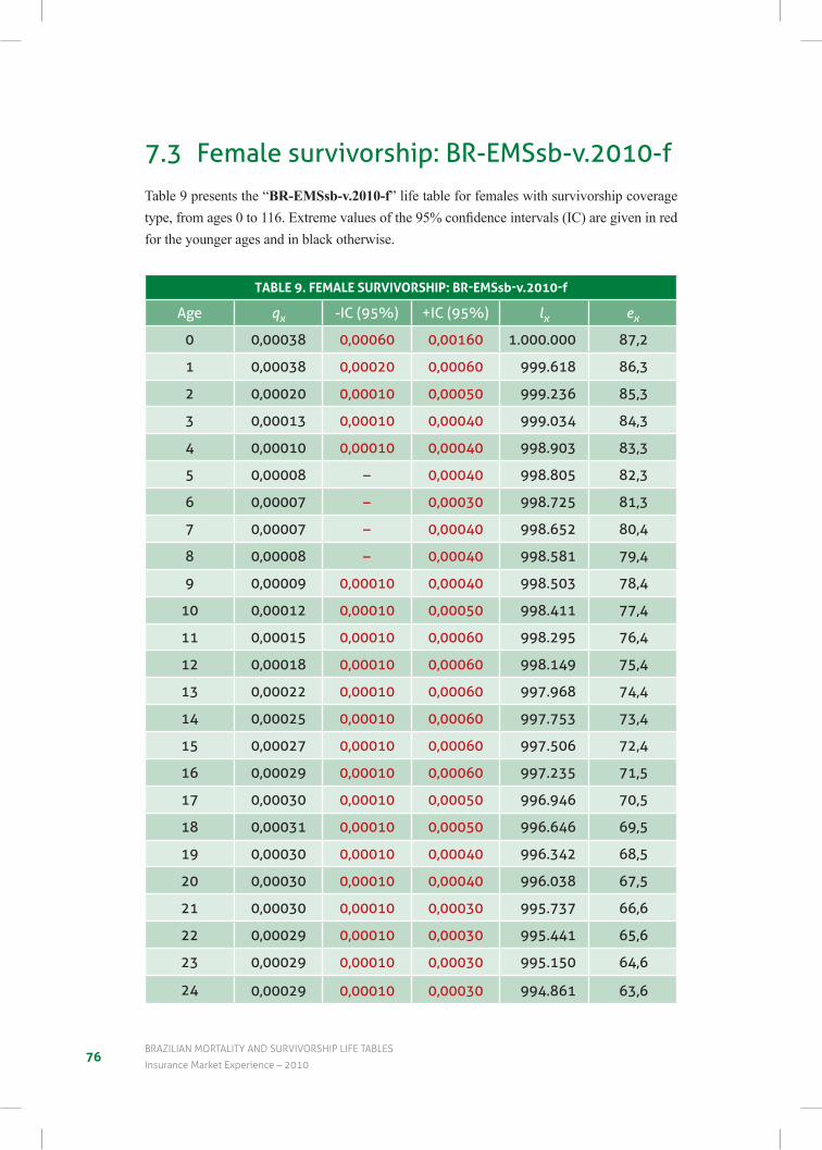
76BraZILIan mOrtaLItY anD surVIVOrsHIp LIFe taBLes
Insurance market experience – 2010
7.3 Female survivorship: Br-eMSsb-v.2010-fTable 9 presents the “BR-EMSsb-v.2010-f” life table for females with survivorship coverage type,fromages0to116.Extremevaluesofthe95%confidenceintervals(IC)aregiveninredfor the younger ages and in black otherwise.
TAble 9. FeMAle SurvivorShip: br-eMSsb-v.2010-f
age qx -ic (95%) +ic (95%) lx ex
0 0,00038 0,00060 0,00160 1.000.000 87,2
1 0,00038 0,00020 0,00060 999.618 86,3
2 0,00020 0,00010 0,00050 999.236 85,3
3 0,00013 0,00010 0,00040 999.034 84,3
4 0,00010 0,00010 0,00040 998.903 83,3
5 0,00008 – 0,00040 998.805 82,3
6 0,00007 – 0,00030 998.725 81,3
7 0,00007 – 0,00040 998.652 80,4
8 0,00008 – 0,00040 998.581 79,4
9 0,00009 0,00010 0,00040 998.503 78,4
10 0,00012 0,00010 0,00050 998.411 77,4
11 0,00015 0,00010 0,00060 998.295 76,4
12 0,00018 0,00010 0,00060 998.149 75,4
13 0,00022 0,00010 0,00060 997.968 74,4
14 0,00025 0,00010 0,00060 997.753 73,4
15 0,00027 0,00010 0,00060 997.506 72,4
16 0,00029 0,00010 0,00060 997.235 71,5
17 0,00030 0,00010 0,00050 996.946 70,5
18 0,00031 0,00010 0,00050 996.646 69,5
19 0,00030 0,00010 0,00040 996.342 68,5
20 0,00030 0,00010 0,00040 996.038 67,5
21 0,00030 0,00010 0,00030 995.737 66,6
22 0,00029 0,00010 0,00030 995.441 65,6
23 0,00029 0,00010 0,00030 995.150 64,6
24 0,00029 0,00010 0,00030 994.861 63,6
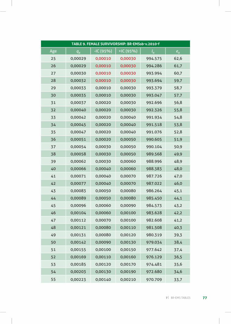
777 BR-EMS TaBlES
TAble 9. FeMAle SurvivorShip: br-eMSsb-v.2010-f
age qx -ic (95%) +ic (95%) lx ex
25 0,00029 0,00010 0,00030 994.575 62,6
26 0,00029 0,00010 0,00030 994.286 61,7
27 0,00030 0,00010 0,00030 993.994 60,7
28 0,00032 0,00010 0,00030 993.694 59,7
29 0,00033 0,00010 0,00030 993.379 58,7
30 0,00035 0,00010 0,00030 993.047 57,7
31 0,00037 0,00020 0,00030 992.696 56,8
32 0,00040 0,00020 0,00030 992.326 55,8
33 0,00042 0,00020 0,00040 991.934 54,8
34 0,00045 0,00020 0,00040 991.518 53,8
35 0,00047 0,00020 0,00040 991.076 52,8
36 0,00051 0,00020 0,00050 990.605 51,9
37 0,00054 0,00030 0,00050 990.104 50,9
38 0,00058 0,00030 0,00050 989.568 49,9
39 0,00062 0,00030 0,00060 988.996 48,9
40 0,00066 0,00040 0,00060 988.383 48,0
41 0,00071 0,00040 0,00070 987.726 47,0
42 0,00077 0,00040 0,00070 987.022 46,0
43 0,00083 0,00050 0,00080 986.264 45,1
44 0,00089 0,00050 0,00080 985.450 44,1
45 0,00096 0,00060 0,00090 984.573 43,2
46 0,00104 0,00060 0,00100 983.628 42,2
47 0,00112 0,00070 0,00100 982.608 41,2
48 0,00121 0,00080 0,00110 981.508 40,3
49 0,00131 0,00080 0,00120 980.319 39,3
50 0,00142 0,00090 0,00130 979.034 38,4
51 0,00155 0,00100 0,00150 977.642 37,4
52 0,00169 0,00110 0,00160 976.129 36,5
53 0,00185 0,00120 0,00170 974.481 35,6
54 0,00203 0,00130 0,00190 972.680 34,6
55 0,00223 0,00140 0,00210 970.709 33,7
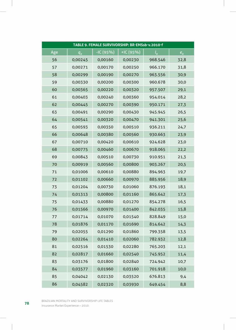
78BraZILIan mOrtaLItY anD surVIVOrsHIp LIFe taBLes
Insurance market experience – 2010
TAble 9. FeMAle SurvivorShip: br-eMSsb-v.2010-f
age qx -ic (95%) +ic (95%) lx ex
56 0,00245 0,00160 0,00230 968.546 32,8
57 0,00271 0,00170 0,00250 966.170 31,8
58 0,00299 0,00190 0,00270 963.556 30,9
59 0,00330 0,00200 0,00300 960.678 30,0
60 0,00365 0,00220 0,00320 957.507 29,1
61 0,00403 0,00240 0,00360 954.014 28,2
62 0,00445 0,00270 0,00390 950.171 27,3
63 0,00491 0,00290 0,00430 945.945 26,5
64 0,00541 0,00320 0,00470 941.301 25,6
65 0,00593 0,00350 0,00510 936.211 24,7
66 0,00648 0,00380 0,00560 930.663 23,9
67 0,00710 0,00420 0,00610 924.628 23,0
68 0,00775 0,00460 0,00670 918.065 22,2
69 0,00843 0,00510 0,00730 910.951 21,3
70 0,00919 0,00560 0,00800 903.267 20,5
71 0,01006 0,00610 0,00880 894.963 19,7
72 0,01102 0,00660 0,00970 885.956 18,9
73 0,01204 0,00730 0,01060 876.193 18,1
74 0,01313 0,00800 0,01160 865.642 17,3
75 0,01433 0,00880 0,01270 854.278 16,5
76 0,01566 0,00970 0,01400 842.035 15,8
77 0,01714 0,01070 0,01540 828.849 15,0
78 0,01876 0,01170 0,01690 814.642 14,3
79 0,02055 0,01290 0,01860 799.358 13,5
80 0,02264 0,01410 0,02060 782.932 12,8
81 0,02516 0,01530 0,02280 765.203 12,1
82 0,02817 0,01660 0,02540 745.952 11,4
83 0,03176 0,01800 0,02840 724.942 10,7
84 0,03577 0,01960 0,03160 701.918 10,0
85 0,04042 0,02130 0,03520 676.813 9,4
86 0,04582 0,02320 0,03930 649.454 8,8
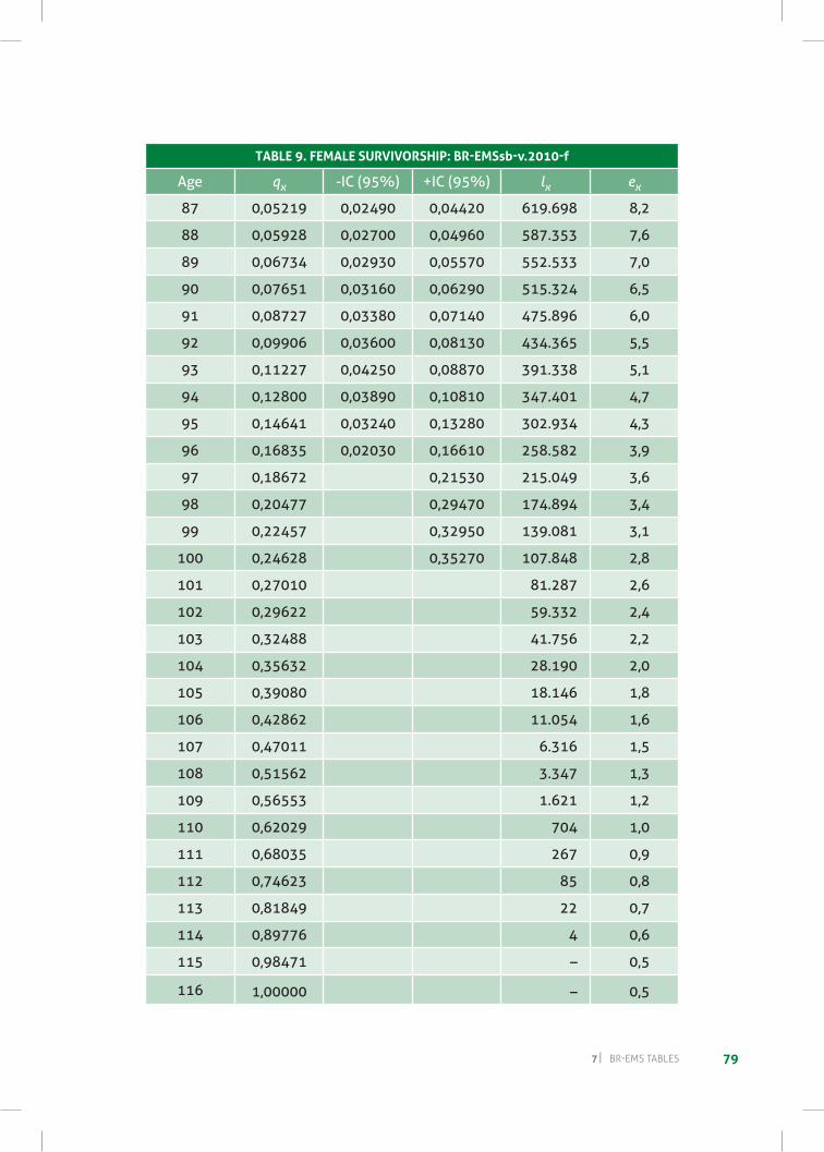
797 BR-EMS TaBlES
TAble 9. FeMAle SurvivorShip: br-eMSsb-v.2010-f
age qx -ic (95%) +ic (95%) lx ex
87 0,05219 0,02490 0,04420 619.698 8,2
88 0,05928 0,02700 0,04960 587.353 7,6
89 0,06734 0,02930 0,05570 552.533 7,0
90 0,07651 0,03160 0,06290 515.324 6,5
91 0,08727 0,03380 0,07140 475.896 6,0
92 0,09906 0,03600 0,08130 434.365 5,5
93 0,11227 0,04250 0,08870 391.338 5,1
94 0,12800 0,03890 0,10810 347.401 4,7
95 0,14641 0,03240 0,13280 302.934 4,3
96 0,16835 0,02030 0,16610 258.582 3,9
97 0,18672 0,21530 215.049 3,6
98 0,20477 0,29470 174.894 3,4
99 0,22457 0,32950 139.081 3,1
100 0,24628 0,35270 107.848 2,8
101 0,27010 81.287 2,6
102 0,29622 59.332 2,4
103 0,32488 41.756 2,2
104 0,35632 28.190 2,0
105 0,39080 18.146 1,8
106 0,42862 11.054 1,6
107 0,47011 6.316 1,5
108 0,51562 3.347 1,3
109 0,56553 1.621 1,2
110 0,62029 704 1,0
111 0,68035 267 0,9
112 0,74623 85 0,8
113 0,81849 22 0,7
114 0,89776 4 0,6
115 0,98471 – 0,5
116 1,00000 – 0,5
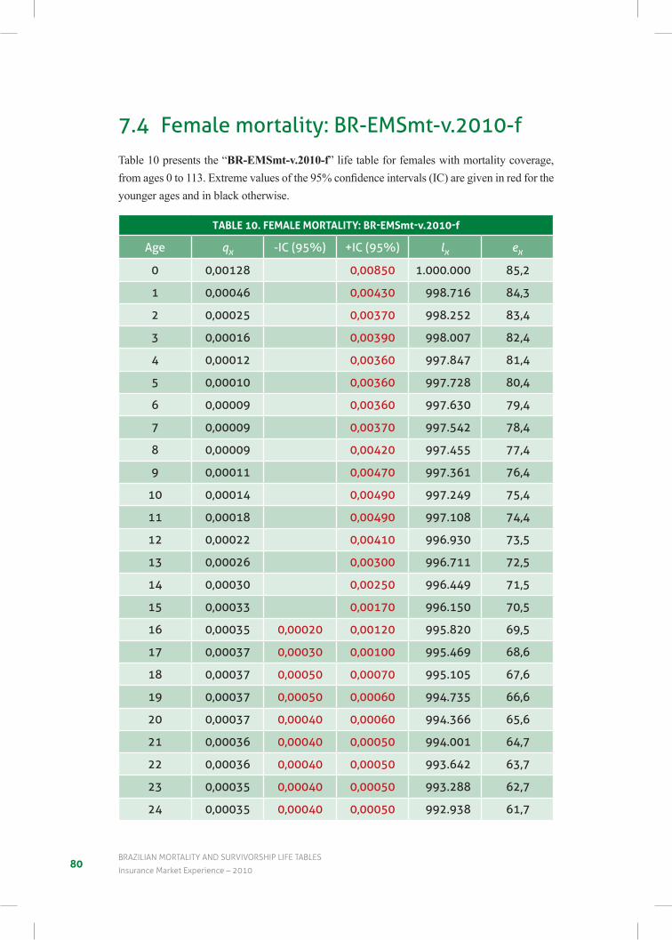
80BraZILIan mOrtaLItY anD surVIVOrsHIp LIFe taBLes
Insurance market experience – 2010
7.4 Female mortality: Br-eMSmt-v.2010-fTable 10 presents the “BR-EMSmt-v.2010-f” life table for females with mortality coverage, fromages0to113.Extremevaluesofthe95%confidenceintervals(IC)aregiveninredfortheyounger ages and in black otherwise.
TAble 10. FeMAle MorTAliTy: br-eMSmt-v.2010-f
age qx -ic (95%) +ic (95%) lx ex
0 0,00128 0,00850 1.000.000 85,2
1 0,00046 0,00430 998.716 84,3
2 0,00025 0,00370 998.252 83,4
3 0,00016 0,00390 998.007 82,4
4 0,00012 0,00360 997.847 81,4
5 0,00010 0,00360 997.728 80,4
6 0,00009 0,00360 997.630 79,4
7 0,00009 0,00370 997.542 78,4
8 0,00009 0,00420 997.455 77,4
9 0,00011 0,00470 997.361 76,4
10 0,00014 0,00490 997.249 75,4
11 0,00018 0,00490 997.108 74,4
12 0,00022 0,00410 996.930 73,5
13 0,00026 0,00300 996.711 72,5
14 0,00030 0,00250 996.449 71,5
15 0,00033 0,00170 996.150 70,5
16 0,00035 0,00020 0,00120 995.820 69,5
17 0,00037 0,00030 0,00100 995.469 68,6
18 0,00037 0,00050 0,00070 995.105 67,6
19 0,00037 0,00050 0,00060 994.735 66,6
20 0,00037 0,00040 0,00060 994.366 65,6
21 0,00036 0,00040 0,00050 994.001 64,7
22 0,00036 0,00040 0,00050 993.642 63,7
23 0,00035 0,00040 0,00050 993.288 62,7
24 0,00035 0,00040 0,00050 992.938 61,7
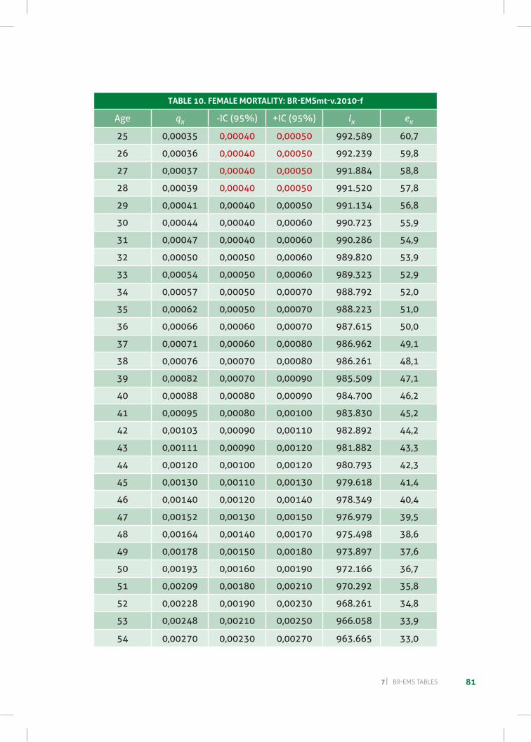
817 BR-EMS TaBlES
TAble 10. FeMAle MorTAliTy: br-eMSmt-v.2010-f
age qx -ic (95%) +ic (95%) lx ex
25 0,00035 0,00040 0,00050 992.589 60,7
26 0,00036 0,00040 0,00050 992.239 59,8
27 0,00037 0,00040 0,00050 991.884 58,8
28 0,00039 0,00040 0,00050 991.520 57,8
29 0,00041 0,00040 0,00050 991.134 56,8
30 0,00044 0,00040 0,00060 990.723 55,9
31 0,00047 0,00040 0,00060 990.286 54,9
32 0,00050 0,00050 0,00060 989.820 53,9
33 0,00054 0,00050 0,00060 989.323 52,9
34 0,00057 0,00050 0,00070 988.792 52,0
35 0,00062 0,00050 0,00070 988.223 51,0
36 0,00066 0,00060 0,00070 987.615 50,0
37 0,00071 0,00060 0,00080 986.962 49,1
38 0,00076 0,00070 0,00080 986.261 48,1
39 0,00082 0,00070 0,00090 985.509 47,1
40 0,00088 0,00080 0,00090 984.700 46,2
41 0,00095 0,00080 0,00100 983.830 45,2
42 0,00103 0,00090 0,00110 982.892 44,2
43 0,00111 0,00090 0,00120 981.882 43,3
44 0,00120 0,00100 0,00120 980.793 42,3
45 0,00130 0,00110 0,00130 979.618 41,4
46 0,00140 0,00120 0,00140 978.349 40,4
47 0,00152 0,00130 0,00150 976.979 39,5
48 0,00164 0,00140 0,00170 975.498 38,6
49 0,00178 0,00150 0,00180 973.897 37,6
50 0,00193 0,00160 0,00190 972.166 36,7
51 0,00209 0,00180 0,00210 970.292 35,8
52 0,00228 0,00190 0,00230 968.261 34,8
53 0,00248 0,00210 0,00250 966.058 33,9
54 0,00270 0,00230 0,00270 963.665 33,0
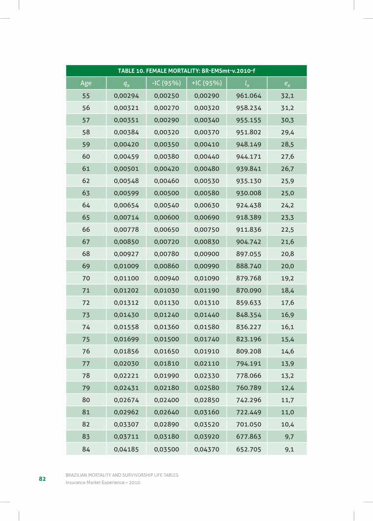
82BraZILIan mOrtaLItY anD surVIVOrsHIp LIFe taBLes
Insurance market experience – 2010
TAble 10. FeMAle MorTAliTy: br-eMSmt-v.2010-f
age qx -ic (95%) +ic (95%) lx ex
55 0,00294 0,00250 0,00290 961.064 32,1
56 0,00321 0,00270 0,00320 958.234 31,2
57 0,00351 0,00290 0,00340 955.155 30,3
58 0,00384 0,00320 0,00370 951.802 29,4
59 0,00420 0,00350 0,00410 948.149 28,5
60 0,00459 0,00380 0,00440 944.171 27,6
61 0,00501 0,00420 0,00480 939.841 26,7
62 0,00548 0,00460 0,00530 935.130 25,9
63 0,00599 0,00500 0,00580 930.008 25,0
64 0,00654 0,00540 0,00630 924.438 24,2
65 0,00714 0,00600 0,00690 918.389 23,3
66 0,00778 0,00650 0,00750 911.836 22,5
67 0,00850 0,00720 0,00830 904.742 21,6
68 0,00927 0,00780 0,00900 897.055 20,8
69 0,01009 0,00860 0,00990 888.740 20,0
70 0,01100 0,00940 0,01090 879.768 19,2
71 0,01202 0,01030 0,01190 870.090 18,4
72 0,01312 0,01130 0,01310 859.633 17,6
73 0,01430 0,01240 0,01440 848.354 16,9
74 0,01558 0,01360 0,01580 836.227 16,1
75 0,01699 0,01500 0,01740 823.196 15,4
76 0,01856 0,01650 0,01910 809.208 14,6
77 0,02030 0,01810 0,02110 794.191 13,9
78 0,02221 0,01990 0,02330 778.066 13,2
79 0,02431 0,02180 0,02580 760.789 12,4
80 0,02674 0,02400 0,02850 742.296 11,7
81 0,02962 0,02640 0,03160 722.449 11,0
82 0,03307 0,02890 0,03520 701.050 10,4
83 0,03711 0,03180 0,03920 677.863 9,7
84 0,04185 0,03500 0,04370 652.705 9,1
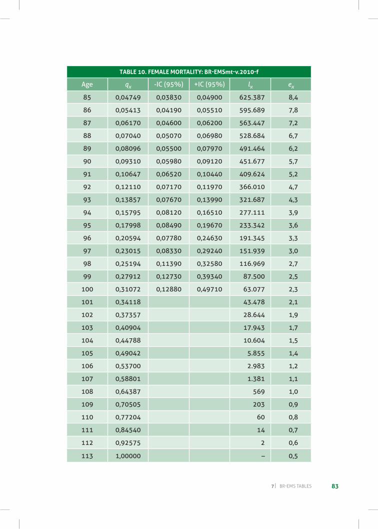
837 BR-EMS TaBlES
TAble 10. FeMAle MorTAliTy: br-eMSmt-v.2010-f
age qx -ic (95%) +ic (95%) lx ex
85 0,04749 0,03830 0,04900 625.387 8,4
86 0,05413 0,04190 0,05510 595.689 7,8
87 0,06170 0,04600 0,06200 563.447 7,2
88 0,07040 0,05070 0,06980 528.684 6,7
89 0,08096 0,05500 0,07970 491.464 6,2
90 0,09310 0,05980 0,09120 451.677 5,7
91 0,10647 0,06520 0,10440 409.624 5,2
92 0,12110 0,07170 0,11970 366.010 4,7
93 0,13857 0,07670 0,13990 321.687 4,3
94 0,15795 0,08120 0,16510 277.111 3,9
95 0,17998 0,08490 0,19670 233.342 3,6
96 0,20594 0,07780 0,24630 191.345 3,3
97 0,23015 0,08330 0,29240 151.939 3,0
98 0,25194 0,11390 0,32580 116.969 2,7
99 0,27912 0,12730 0,39340 87.500 2,5
100 0,31072 0,12880 0,49710 63.077 2,3
101 0,34118 43.478 2,1
102 0,37357 28.644 1,9
103 0,40904 17.943 1,7
104 0,44788 10.604 1,5
105 0,49042 5.855 1,4
106 0,53700 2.983 1,2
107 0,58801 1.381 1,1
108 0,64387 569 1,0
109 0,70505 203 0,9
110 0,77204 60 0,8
111 0,84540 14 0,7
112 0,92575 2 0,6
113 1,00000 – 0,5
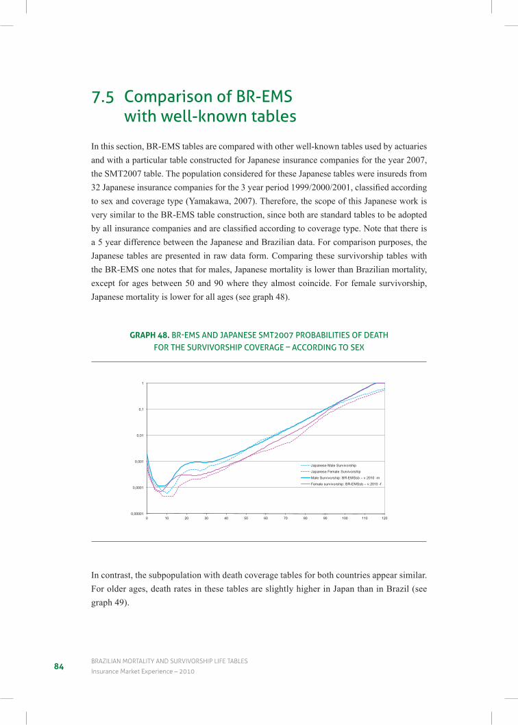
84BraZILIan mOrtaLItY anD surVIVOrsHIp LIFe taBLes
Insurance market experience – 2010
7.5 comparison of Br-eMS with well-known tables
In this section, BR-EMS tables are compared with other well-known tables used by actuaries and with a particular table constructed for Japanese insurance companies for the year 2007, the SMT2007 table. The population considered for these Japanese tables were insureds from 32Japaneseinsurancecompaniesforthe3yearperiod1999/2000/2001,classifiedaccordingto sex and coverage type (Yamakawa, 2007). Therefore, the scope of this Japanese work is very similar to the BR-EMS table construction, since both are standard tables to be adopted byallinsurancecompaniesandareclassifiedaccordingtocoveragetype.Notethatthereisa 5 year difference between the Japanese and Brazilian data. For comparison purposes, the Japanese tables are presented in raw data form. Comparing these survivorship tables with the BR-EMS one notes that for males, Japanese mortality is lower than Brazilian mortality, except for ages between 50 and 90 where they almost coincide. For female survivorship, Japanese mortality is lower for all ages (see graph 48).
grAPH 48. BR-EMS AND JAPANESE SMT2007 PROBABILITIES OF DEATHFor the SUrvivorShiP coveraGe – accordinG to SeX
0,00001
0,0001
0,001
0,01
0,1
1
0 10 20 30 40 50 60 70 80 90 100 110 120
BR-EMS AND JAPANESE SMT2007 PROBABILITIES OF DEATH FOR THE SURVIVORSHIP COVERAGE – ACCORDING TO SEX
Japanese Male Survivorship
Japanese Female Survivorship
Male Survivorship: BR-EMSsb – v.2010 -m
Female survivorship: BR-EMSsb – v.2010 -f
In contrast, the subpopulation with death coverage tables for both countries appear similar. For older ages, death rates in these tables are slightly higher in Japan than in Brazil (see graph 49).
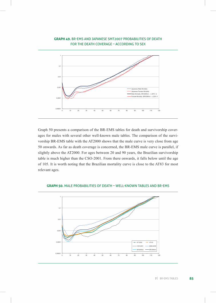
857 BR-EMS TaBlES
grAPH 49. BR-EMS AND JAPANESE SMT2007 PROBABILITIES OF DEATHFor the death coveraGe – accordinG to SeX
0,00001
0,0001
0,001
0,01
0,1
1
0 10 20 30 40 50 60 70 80 90 100 110 120
BR-EMS AND JAPANESE SMT2007 PROBABILITIES OF DEATH FOR THE DEATH COVERAGE –ACCORDING TO SEX
Japanese Male Mortality
Japanese Female Mortality
Male Mortality: BR-EMSmt – v.2010 -m
Female Mortality: BR-EMSmt – v.2010 -f
Graph 50 presents a comparison of the BR-EMS tables for death and survivorship cover-ages for males with several other well-known male tables. The comparison of the survi-vorship BR-EMS table with the AT2000 shows that the male curve is very close from age 50 onwards. As far as death coverage is concerned, the BR-EMS male curve is parallel, if slightly above the AT2000. For ages between 20 and 90 years, the Brazilian survivorship table is much higher than the CSO-2001. From there onwards, it falls below until the age of 105. It is worth noting that the Brazilian mortality curve is close to the AT83 for most relevant ages.
grAPH 50. Male ProBaBilitieS oF death – WELL-KNOWN TABLES AND BR-EMS
0,00001
0,0001
0,001
0,01
0,1
1
0 10 20 30 40 50 60 70 80 90 100 110 120
MALE PROBABILITIES OF DEATH – WELL-KNOWN TABLES AND BR-EMS
AT-2000 AT-83
CSO-2001 IBGE-2006
BR-EMSsb BR-EMSmt
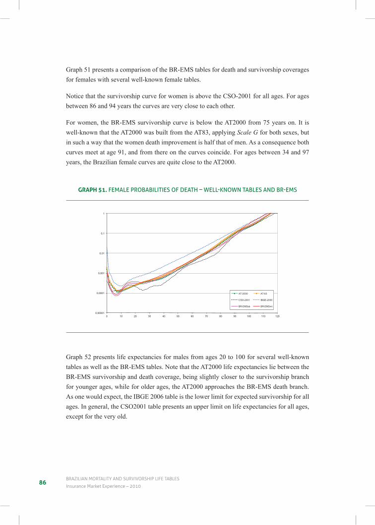
86BraZILIan mOrtaLItY anD surVIVOrsHIp LIFe taBLes
Insurance market experience – 2010
Graph 51 presents a comparison of the BR-EMS tables for death and survivorship coverages for females with several well-known female tables.
Notice that the survivorship curve for women is above the CSO-2001 for all ages. For ages between 86 and 94 years the curves are very close to each other.
For women, the BR-EMS survivorship curve is below the AT2000 from 75 years on. It is well-known that the AT2000 was built from the AT83, applying Scale G for both sexes, but in such a way that the women death improvement is half that of men. As a consequence both curves meet at age 91, and from there on the curves coincide. For ages between 34 and 97 years, the Brazilian female curves are quite close to the AT2000.
grAPH 51. FeMale ProBaBilitieS oF death – WELL-KNOWN TABLES AND BR-EMS
0,00001
0,0001
0,001
0,01
0,1
1
0 10 20 30 40 50 60 70 80 90 100 110 120
FEMALE PROBABILITIES OF DEATH – WELL-KNOWN TABLES AND BR-EMS
AT-2000 AT-83
CSO-2001 IBGE-2006
BR-EMSsb BR-EMSmt
Graph 52 presents life expectancies for males from ages 20 to 100 for several well-known tables as well as the BR-EMS tables. Note that the AT2000 life expectancies lie between the BR-EMS survivorship and death coverage, being slightly closer to the survivorship branch for younger ages, while for older ages, the AT2000 approaches the BR-EMS death branch. As one would expect, the IBGE 2006 table is the lower limit for expected survivorship for all ages. In general, the CSO2001 table presents an upper limit on life expectancies for all ages, except for the very old.
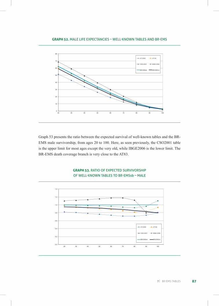
877 BR-EMS TaBlES
grAPH 52. Male liFe eXPectancieS – WELL-KNOWN TABLES AND BR-EMS
0
10
20
30
40
50
60
70
80
20 30 40 50 60 70 80 90 100
MALE LIFE EXPECTANCIES – WELL-KNOWN TABLES AND BR-EMS
AT-2000 AT-83
CSO-2001 IBGE-2006
BR-EMSsb BR-EMSmt
Graph 53 presents the ratio between the expected survival of well-known tables and the BR-EMS male survivorship, from ages 20 to 100. Here, as seen previously, the CSO2001 table is the upper limit for most ages except the very old, while IBGE2006 is the lower limit. The BR-EMS death coverage branch is very close to the AT83.
grAPH 53. ratio oF eXPected SUrvivorShiP OF WELL-KNOWN TABLES TO BR-EMSsb – Male
0,0
0,2
0,4
0,6
0,8
1,0
1,2
1,4
20 30 40 50 60 70 80 90 100
RATIO OF EXPECTED SURVIVORSHIP OF WELL-KNOWN TABLES TO BR-EMSsb – MALE
AT-2000 AT-83
CSO-2001 IBGE-2006
BR-EMSsb BR-EMSmt
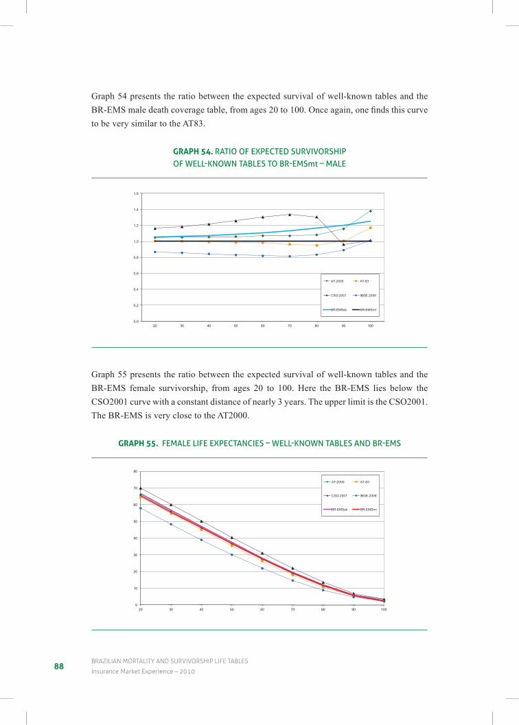
88BraZILIan mOrtaLItY anD surVIVOrsHIp LIFe taBLes
Insurance market experience – 2010
Graph 54 presents the ratio between the expected survival of well-known tables and the BR-EMSmaledeathcoveragetable,fromages20to100.Onceagain,onefindsthiscurveto be very similar to the AT83.
grAPH 54. ratio oF eXPected SUrvivorShiP OF WELL-KNOWN TABLES TO BR-EMSmt – Male
0,0
0,2
0,4
0,6
0,8
1,0
1,2
1,4
1,6
20 30 40 50 60 70 80 90 100
RATIO OF EXPECTED SURVIVORSHIP OF WELL-KNOWN TABLES TO BR-EMSmt – MALE
AT-2000 AT-83
CSO-2001 IBGE-2006
BR-EMSsb BR-EMSmt
Graph 55 presents the ratio between the expected survival of well-known tables and the BR-EMS female survivorship, from ages 20 to 100. Here the BR-EMS lies below the CSO2001 curve with a constant distance of nearly 3 years. The upper limit is the CSO2001. The BR-EMS is very close to the AT2000.
grAPH 55. FeMale liFe eXPectancieS – WELL-KNOWN TABLES AND BR-EMS
0
10
20
30
40
50
60
70
80
20 30 40 50 60 70 80 90 100
FEMALE LIFE EXPECTANCIES – WELL-KNOWN TABLES AND BR-EMS
AT-2000 AT-83
CSO-2001 IBGE-2006
BR-EMSsb BR-EMSmt
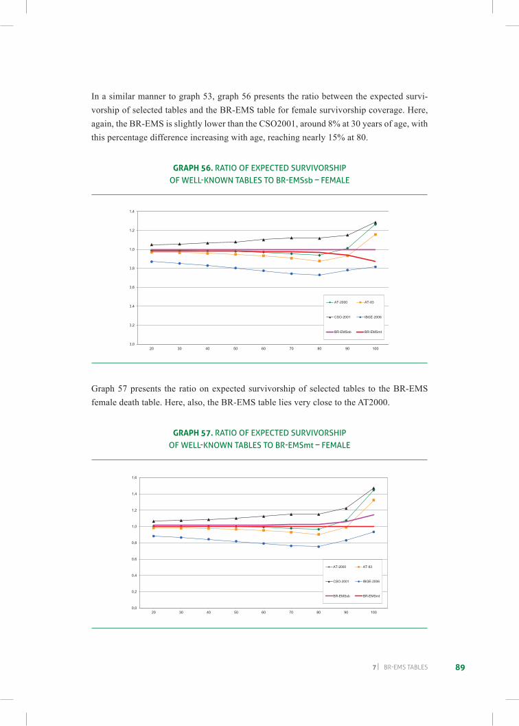
897 BR-EMS TaBlES
In a similar manner to graph 53, graph 56 presents the ratio between the expected survi-vorship of selected tables and the BR-EMS table for female survivorship coverage. Here, again, the BR-EMS is slightly lower than the CSO2001, around 8% at 30 years of age, with this percentage difference increasing with age, reaching nearly 15% at 80.
grAPH 56. ratio oF eXPected SUrvivorShiPOF WELL-KNOWN TABLES TO BR-EMSsb – FeMale
0,0
0,2
0,4
0,6
0,8
1,0
1,2
1,4
20 30 40 50 60 70 80 90 100
RAZÃO DA ESPERANÇA DE SOBREVIDA – TÁBUAS SELECIONADAS E BR-EMSsb – MULHERES
AT-2000 AT-83
CSO-2001 IBGE-2006
BR-EMSsb BR-EMSmt
Graph 57 presents the ratio on expected survivorship of selected tables to the BR-EMS female death table. Here, also, the BR-EMS table lies very close to the AT2000.
grAPH 57. ratio oF eXPected SUrvivorShiPOF WELL-KNOWN TABLES TO BR-EMSmt – FeMale
0,0
0,2
0,4
0,6
0,8
1,0
1,2
1,4
1,6
20 30 40 50 60 70 80 90 100
RATIO OF EXPECTED SURVIVORSHIP OF WELL-KNOWN TABLES TO BR-EMSmt – FEMALE
AT-2000 AT-83
CSO-2001 IBGE-2006
BR-EMSsb BR-EMSmt
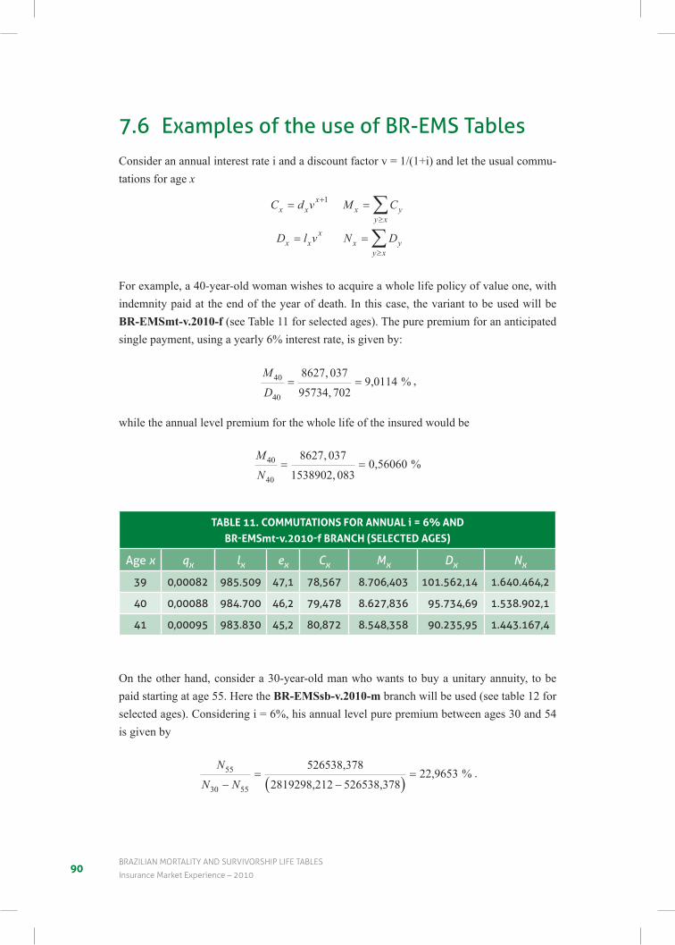
90BraZILIan mOrtaLItY anD surVIVOrsHIp LIFe taBLes
Insurance market experience – 2010
7.6 examples of the use of Br-eMS tablesConsider an annual interest rate i and a discount factor v = 1/(1+i) and let the usual commu-tations for age x
C d v M C
D l v N D
x xx
x yy x
x xx
x yy x
= =
= =
+
≥
≥
∑
∑
1
For example, a 40-year-old woman wishes to acquire a whole life policy of value one, with indemnity paid at the end of the year of death. In this case, the variant to be used will be BR-EMSmt-v.2010-f (see Table 11 for selected ages). The pure premium for an anticipated single payment, using a yearly 6% interest rate, is given by:
M
D40
40
8627 037
95734 702= =
,
,%9,0114 ,
while the annual level premium for the whole life of the insured would be
M
N40
40
8627 037
1538902 083= =
,
,%0,56060
TABLe 11. CoMMuTATIons for AnnuAL i = 6% AnD br-eMSmt-v.2010-f BrAnCH (seLeCTeD Ages)
age x qx lx ex Cx Mx Dx Nx
39 0,00082 985.509 47,1 78,567 8.706,403 101.562,14 1.640.464,2
40 0,00088 984.700 46,2 79,478 8.627,836 95.734,69 1.538.902,1
41 0,00095 983.830 45,2 80,872 8.548,358 90.235,95 1.443.167,4
On the other hand, consider a 30-year-old man who wants to buy a unitary annuity, to be paid starting at age 55. Here the BR-EMSsb-v.2010-m branch will be used (see table 12 for selected ages). Considering i = 6%, his annual level pure premium between ages 30 and 54 is given by
N
N N55
30 55−=
−=
( )526538,378
2819298,212 526538,37822,9653 % .
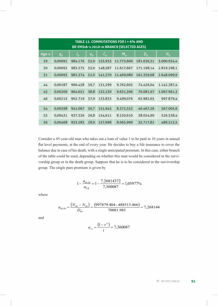
917 BR-EMS TaBlES
TABLe 12. CoMMuTATIons for i = 6% AnD br-eMSsb-v.2010-m BrAnCH (seLeCTeD Ages)
age x qx lx ex Cx Mx Dx Nx
29 0,00091 984.176 53,9 155,933 11.773,600 181.636,31 3.000.934,4
30 0,00092 983.275 53,0 148,587 11.617,667 171.198,14 2.819.298,1
31 0,00093 982.374 52,0 141,570 11.469,080 161.359,68 2.648.099,9
44 0,00187 966.458 39,7 131,299 9.762,605 74.426,04 1.142.387,4
45 0,00200 964.651 38,8 132,230 9.631,306 70.081,97 1.067.961,3
46 0,00215 962.719 37,9 133,833 9.499,076 65.982,65 997.879,4
54 0,00398 941.067 30,7 151,943 8.372,553 40.467,26 567.005,6
55 0,00431 937.326 29,8 154,611 8.220,610 38.024,90 526.538,4
56 0,00468 933.283 28,9 157,698 8.065,999 35.717,82 488.513,5
Consider a 45-year-old man who takes out a loan of value 1 to be paid in 10 years in annual flatlevelpayments,attheendofeveryyear.Hedecidestobuyalifeinsurancetocoverthebalance due in case of his death, with a single anticipated premium. In this case, either branch of the table could be used, depending on whether this man would be considered in the survi-vorship group or in the death group. Suppose that he is to be considered in the survivorship group. The single pure premium is given by
%05977,1
360087,77.2681437211
|01
10:45 =−=−aa
where
( ) ( ) 268144,770081.985
488513.466-997879.40445
564610:45 ==
−=
DNNa
and
( ) 360087,71 10
|01=
−=
iva


93
references
ABDOUG, B.; GHOUDI, K. and KHOUDRAJI, A. Non-Parametric Estimation of the Limit Dependence Function of Multivariate Extremes. Extremes, 2(3):245-268, 1999.
Abid, Ahmed D. & Kamhawey, Ahmed A. & Alsalloum, Othman I. (2005). Graduating the Saudi Crude Mortality Rates and Constricting their Monetary Tables, ASTIN Colloquium, Zurich, Switzerland, 5-7 September.
ANDREEV, Kirill F. and VAUPEL, James W. Patterns of Mortality Improvement over Age and Time in Developed Countries: Estimation, Presentation and Implications for Mortality Forecasting. Web February 12, 2005
AON CONSULTING. Implications of the Adoption of the 2001 CSO: A Research Report from Aon Insurance Consulting Service, September, 2002.
BALKEMA, A.A. and de HAAN, L. Residual life Time at Great Age. Annals of Probability, 2:792-804, 1974.
BARBI, Elisabetta. Assessing the Rate of Ageing of the Human Population, MPIDR WORKING PAPER WP 2003-008, MARCH 2003
BELTRÃO, Kaizô Iwakami; SUGAHARA, Sonoe. Taxas de Mortalidade no Setor de Seguros – 1998-2000. Estimativas e Comparações com Tábuas do Mercado. Rio de Janeiro, Funenseg 250 pp, 2005.
BELTRÃO, Kaizô Iwakami; SUGAHARA, Sonoe. Tábua de Mortalidade para os Funcionários Públicos Civis Federais do Poder Executivo por Sexo e Escolaridade: Comparação com Tábuas do Mercado. TD 3, ENCE/IBGE, Rio de Janeiro, novembro de 2002b.
BELTRÃO, Kaizô Iwakami; SUGAHARA, Sonoe. Mortality Rates in the Brazilian Insurance Market: a Comparison. Brazilian Journal of Probability and Statistics, 19,2, December 2005.
94BraZILIan mOrtaLItY anD surVIVOrsHIp LIFe taBLes
Insurance market experience – 2010
BENNETT, Neil G; HORIUCHI, Shiro. Estimating the Completeness of Death Registration in a Closed Population: current items. Population Index, Princeton, NJ, USA, pp. 207-222, 1981.
BLOOMFIELD, D. S. F. & HABERMAN, S. Graduation: Some Experiments with Kernel Methods. JIA 114 (1987) 339-369
BONGAARTS, John& FEENEY,Griffith.How Long Do We Live? Population Council. Policy Research Division, Working Paper Nº 156, 2002.
BONGAARTS,John&FEENEY,GriffithEstimating Mean Lifetime. Population Council. Policy Research Division, Working Paper No. 179, 2003.
BOWERS, N. L.; GERBER, H.U.; HICKMAN, J. C. and NESBITT, C. J. Actuarial Mathematics. Society of Actuaries, Itasca, Illinois, 1986.
BRASS, William. Methods For Estimating Fertility And Mortality From Limited and Defective Data. Chapell Hill, North Carolina, Carolina Population Center, Laboratories for Population Studies, 1975.
BRIAN, Eric; ROHRBASSER, Jean-Marc; THÉRÉ, Christine; et VÉRON, Jacques. La dureedevie:Histoireetcalcul–especulationssurlaviehumaineetcrisefinancierealafinduXVIII-emesiecle. l’INED – DOCUMENTS DE TRAVAIL, 109, 2002.
BRILLINGER,D.R.AJustificationofSomeCommonLawsofMortality.Transactionsofthe Society of Actuaries, 116-126, 1961.
CARRIERE, Jacques F. Parametric Models for Life Tables. Transactions of Society of Actuaries, 1992 vol. 44.
CARRIERE, Jacques F. A Select and Ultimate Parametric Model. Transactions of Society of Actuaries, 1994 vol. 46.
COALE, Ansley J. &Demeny Paul, Regional Model Life Tables and Stable Population, Princeton UP, Princeton, NJ, 1966.
Continuous Mortality Investigation/Mortality Committee. The Graduation of the CMI 1999-2002 Mortality Experience: Feedback on Working Paper 8 and Proposed Assured Lives Graduations. CMI Working Paper 12, April 2005.
_________________________________. Projecting Future Mortality: Towards a Proposal for a Stochastic Methodology. CMI Working Paper 15, July 2005.
95reFerences
_________________________________. The Graduation of the CMI 1999-2002 Mortality Experience: Proposed Annuitant and Pensioner Graduations. CMI Working Paper 16, September 2005.
_________________________________. The Graduation of the CMI 1999-2002 Mortality Experience: Final “00” Series Mortality Tables – Assured Lives. CMI Working Paper 21, July 2006.
_________________________________. The Graduation of the CMI 1999-2002 Mortality Experience: Final “00” Series Mortality Tables – Annuitants and Pensioners. CMI Working Paper 22, July 2006.
_________________________________. Stochastic Projection Methodologies: Lee-Carter Model Features, Example Results and Implications. CMI Working Paper 25, April 2007.
_________________________________. Extensions to Younger Ages of the “00” Series Pensioner Tables of mortality. CMI Working Paper 26, April 2007.
_________________________________. The “Library” of Mortality Projections. CMI Working Paper 27, July 2007.
Copas, J.B. & Haberman, M. A. (1983). Non-Parametric Graduation Using Kernel Methods. Journal of the Institute of Actuaries, 110, 135-156.
COURBAGE, Youssef; FARGUES, Philippe. A Method for Deriving Mortality Estimates from Incomplete Vital Statistics. Population Studies, 33, 1, 1979.
CURRIE, Iain; KIRKBY, James; DURBAN, Maria; and EILERS, Paul. Smooth Lee-Carter Models and Beyond. International Centre for Mathematical Sciences, Edinburgh, September 2004.
DAVID, F. N. Games, Gods and Gambling – A History of Probability and Statistical Ideas, Dow Publication Inc., Mineole, NY, USA, 1998.
DOBSON, Annettte J. Introduction to Statistical Modeling. London; New York: Champman and Hall, 1983.
DUCHENE, Josianne; WUNSCH, Guillaume. Population Aging and the Limits to Human Life. Working paper n.1. Département de Démographie, Université Catholique de Louvain, Bruxelles, Belgique, août 1988.
HELIGMAN, Larry; POLLARD, J. H.The Age Pattern of Mortality. Readings in Population Research Methodology, v.2, pp. 97-104, 1980.
96BraZILIan mOrtaLItY anD surVIVOrsHIp LIFe taBLes
Insurance market experience – 2010
JOSEPH, A.W. The Whittaker-Henderson Method of Graduation. Journal of the Institute of Actuaries, 99-114, 1952.
KIMELDORF, G. S. and JONES, D. A. Bayesian Graduation. Transactions of Society of Actuaries, v. 19, 1967, p 66-112.
KOSTAKI, A. & PANOUSIS, V. Expanding an Abridged Life Table, Demographic Research, vol.5, article 1, 2001.
LAUDERDALE Diane S. & KESTENBAUM Bert, Mortality Rates of Elderly Asian American Populations, Demography, 39, 3, August 2002.
LEDERMANN, S. & BREAS, Jean. “Les dimensions de la mortalité”, Population, 14, 4, 1959.
LEE, Ronald D.; CARTER, Lawrence R. Modeling and Forecasting the Time Series of US Mortality. Journal of the American Statistical Association, 87: pp.659-71, 1992.
LEVY, A. & ZACS, A. Dynamical Life Tables, Technion, IIT, Haifa, 2002.
MACCULLAGH, P., NELDER, J. A. Generalized Linear Models. London: Chapman and Hall, 1983.
NAVATHE, S., ELMASRI, R., “Fundamentals of Database Systems”, Addison Wesley; 6th edition; 2011
ROLAND, Rau; SOROKO, Eugeny; JASILIONIS, Domantas; VAUPEL, James W. 10 Years After Kannisto. Further Evidence for Mortality Decline at Advanced Ages in Developed Countries, MPIDR WORKING PAPER WP 2006-033 October 2006.
RENSHAW,A.E. and HABERMAN,S. Modelling for Mortality Reduction Factors. Actuarial Research Paper, v. 127. London: City University, 2000.
ROSENWAIKEIra&STONE,LeslieF.VerificationoftheAgesofSupercentenariansintheUnited States: results of a matching study, Demography, vol. 40, pp.727-739, 2003.
SEAL, H.L. Tests of a Mortality Table Graduation, Journal of The Institute Of Actuaries, 5-67, 1953.
TUKEY, JOHN W (1977). Exploratory Data Analysis. Addison-Wesley.
UNITED NATIONS, Manual X: Indirect Techniques for Demographic Estimation, New York, 1983.
UNITED NATIONS, Model Life Tables for Developing Countries, New York, 1983.
97reFerences
VALLIN, J., MESLÉ,F. Trends in Mortality and Differential Mortality, Population Studies No. 36, Council of Europe Publishing, ISBN 92-871-4725-6, December 2001; Inwww.coe.int/t/e/social_cohesion/population/N%C2%B036_Trends_in_mortality.pdf
VAUPEL, James W. et al. Biodemographic Trajectories of Longevity. Science, vol. 280, pp.855-60, 1998.
VAUPEL, James W. Post-Darwinian Longevity, MPIDR Working paper wp 2002-043, September 2002
Verrall,R.(1996).AUnifiedFrameworkforGraduation,ActuarialResearchPaper91,CityUniversity, London, UK.
WACHETER, Kenneth W.; FINCH, Caleh E. eds. Between Zeus and the Salmon – The Biodemography of Longevity. National Academy Press, Washington D.C., 1997.
YAMAKAWA, Tatsuhiro. The Standard Mortality Table 2007. Tokyo: Institute of Actuaries of Japan, 2007. In www.actuaries.jp/eaac14th/pdf/session/06_2P_Yamakawa Tatsuhiro_18Revised.pdf


The Escola Nacional de Seguros, conscious of its environmental and social responsibilities, uses FSC® (Forest Stewardship Council) certified paper throughout this book. FSC certification ensures a raw material is soured from forests considered to be socially, environmentally and economically appropriate, printed by
Gráfica Stamppa – certified within the FSC custody chain.


![Savini Wheels Catalog - CARiD.com · M Wheel Builder SAVIN] i zer 3 rlossin - Savin' -J7c Savini Styling proud to announce the newest ... PORSCHE RANGE ROVER ROLLS ROYCE SV -35 Click](https://img.pdfslide.us/doc/110x75/5bf9909009d3f2e7208c9244/savini-wheels-catalog-caridcom-m-wheel-builder-savin-i-zer-3-rlossin-savin.jpg)