Embed Size (px)
Citation preview
Avoided Energy Supply Costs in New England
Prepared for:
Avoided-Energy-Supply-Component (AESC) Study Group
Prepared by:
Final Report
December 23, 2005
0
Avoided Energy Supply C
Note: This report was produced by ICF Consulting (ICF) in accordance with agreements made with individual members of the AESC Study Group. (Client). Client’s use of this report is subject to the terms of those agreements.
osts • Prepared by ICF Resources LLC 1
Avoided Energy Supply Costs • Prepared by ICF Resources LLC i
Table of Contents EXECUTIVE SUMMARY .........................................................................................................................................1
Study Background.....................................................................................................................................................1
The Modeling Approach...........................................................................................................................................1
Summary of Results..................................................................................................................................................2
CHAPTER ONE: AVOIDED GAS COSTS...........................................................................................................17
Summary of Avoided Gas Costs.............................................................................................................................17
Overview of New England Gas Market ..................................................................................................................20
Methodology...........................................................................................................................................................27
Henry Hub Prices....................................................................................................................................................27
Summer/Winter Differentials..................................................................................................................................29
Delivery Costs to New England..............................................................................................................................30
Retail Customer Avoided Costs..............................................................................................................................37
Comparison with Previous Avoided Cost Study.....................................................................................................38
Avoided Gas Costs in Vermont ..............................................................................................................................38
Avoided Gas Costs for Power Generation ..............................................................................................................40
CHAPTER TWO: WHOLESALE ELECTRICITY PRICE MODELING METHODOLOGY, NEW ENGLAND POWER MARKET AND KEY ASSUMPTIONS OVERVIEW......................................................41
Introduction.............................................................................................................................................................41
Wholesale Price Forecasting Methodology ............................................................................................................41
The New England Power Market............................................................................................................................45
Wholesale Market Modeling Assumptions Utilized in the Avoided Cost Analysis ...............................................67
CHAPTER THREE: AVOIDED ELECTRIC SUPPLY COMPONENT COST FORECAST RESULTS.......89
Wholesale Power Prices..........................................................................................................................................90
Transmission and Distribution Adders ...................................................................................................................99
Retail Price Adders ...............................................................................................................................................101
Comparison to 2003 Study....................................................................................................................................103
CHAPTER FOUR: OTHER FUEL AVOIDED COSTS ....................................................................................108
Avoided Energy Supply Costs • Prepared by ICF Resources LLC ii
Crude Oil Price Forecast.......................................................................................................................................108
Distillate Fuel Prices in New England ..................................................................................................................110
New England Residual Fuel Prices: No. 6 and No. 4 ...........................................................................................111
Kerosene Prices in New England..........................................................................................................................111
New England Propane Pricing ..............................................................................................................................111
Firewood in New England ....................................................................................................................................111
CHAPTER FIVE: AVOIDED TRANSMISSION AND DISTRIBUTION CAPACITY COSTS....................118
Summary of Transmission and Distribution Avoided Capacity Cost Calculator..................................................118
CHAPTER SIX: DEMAND REDUCTION INDUCED PRICE EFFECTS......................................................129
DRIPE Benefits ....................................................................................................................................................129
DRIPE Light Benefits ...........................................................................................................................................134
Methodology.........................................................................................................................................................136
APPENDIX ONE: ELECTRIC POWER COSTING PERIODS........................................................................148
Introduction...........................................................................................................................................................148
Exhibit A1-3: Estimated Savings Differences in MA: Recommended and Adopted Costing Periods ................149
Energy Costing Period Analysis ...........................................................................................................................149
Capacity Value Period Analysis ...........................................................................................................................154
APPENDIX TWO: DETAILED ELECTRIC ENERGY AVOIDED COST TABLES.....................................158
Table Structure and Terminology .........................................................................................................................158
APPENDIX THREE: SOURCES ..........................................................................................................................206
Avoided Energy Supply Costs • Prepared by ICF Resources LLC 1
Executive Summary
Study Background
As part of an ongoing review of expected avoided supply costs in New England, ICF Consulting (ICF) was retained by the 2005 Avoided-Energy-Supply-Component (AESC) Study Group to provide an analysis of the energy supply costs (electricity, natural gas, fuel oil, and wood) potentially avoided through the implementation of energy efficiency programs in New England. Ratepayer funds support energy-efficiency programs, which focus on reducing electricity and/or gas consumption. This study is intended to support energy-efficiency program planning and development by program administrators participating in the AESC group. In addition, this study is intended for use by AESC group members to support regulatory filings.
The primary target of the energy efficiency programs are electricity and gas use and are hence the primary focus of this report. Other fuels also considered are propane, residual fuel oil, distillate fuel oil, kerosene for heating, and wood.
The AESC Study Group includes a broad spectrum of electric and gas utilities or their representatives from Massachusetts, New Hampshire, Vermont, Rhode Island, Connecticut, and Maine.
The sponsors of this project include: Berkshire Gas Company, Keyspan Energy Delivery New England (Boston Gas Company, Essex Gas Company, and Colonial Gas Company), Cape Light Compact, National Grid USA (Massachusetts Electric Company, New England Gas Company, NiSource Inc., NSTAR Electric & Gas Company, Northeast Utilities (Western Massachusetts Electric and Public Service of New Hampshire), Unitil (Fitchburg Gas and Electric Light Company, United Illuminating, Concord Electric Company and Exeter & Hampton Electric Company), the State of Maine, and the State of Vermont. Additional members of the Study Group include Connecticut Energy Conservation Management Board, Massachusetts Department of Telecommunications and Energy, Massachusetts Division of Energy Resources, Massachusetts Low-Income Energy Affordability Network (LEAN) and other Non-Utility Parties, New Hampshire Public Utilities Commission, and Rhode Island Division of Public Utilities and Carriers.
The Modeling Approach
This analysis utilizes a detailed and integrated fundamentals modeling approach combined with actual market data to estimate the supply costs considered to be avoidable. To provide projections of wholesale or spot market fuel market prices and wholesale energy and capacity prices, ICF utilized a fundamentals based modeling approach for the gas and power wholesale or spot markets. ICF further estimated the costs considered avoidable for retail power market services and gas services through estimating actual cost expenditures for these services. Avoided costs for other fuels were estimated in conjunction with the natural gas market analysis. Transmission and distribution avoidable costs were considered under the electricity sector portion of this analysis.
To project wholesale market conditions going forward, ICF relied on the combination of the
Avoided Energy Supply Costs • Prepared by ICF Resources LLC 2
NANGAS® natural gas market model to forecast delivered to New England market pricing and the IPM® power market model to forecast near- and long-term power market conditions. IPM® considers the entire time horizon (2005 – 2040) to determine the optimal distribution and use of generation and transmission resources including the potential retirement, retrofitting, or addition of capacity. Similarly, NANGAS® is a fundamentals based model capturing reservoir level detail on the supply side and reflecting the demand side fundamentals through sectoral demand estimates and representation of the North American pipeline system.
Prior studies were commissioned by the AESC Study Group in 1999, 2001, and 2003. A comparison of currently available information from the most recent analysis is provided within this report. Sections of this analysis were not previously performed under the 2003 vintage study and will not be directly compared.
Among the Study Group’s objectives for this analysis was to revisit the estimation of marginal supply costs avoided by conservation savings, based on projected demand, available sources, and fuel prices for marginal supply sources, while also including the impacts of locational marginal pricing recently added to the New England electric market and locational capacity markets expected to be in place in New England shortly.
Summary of Results
Natural Gas
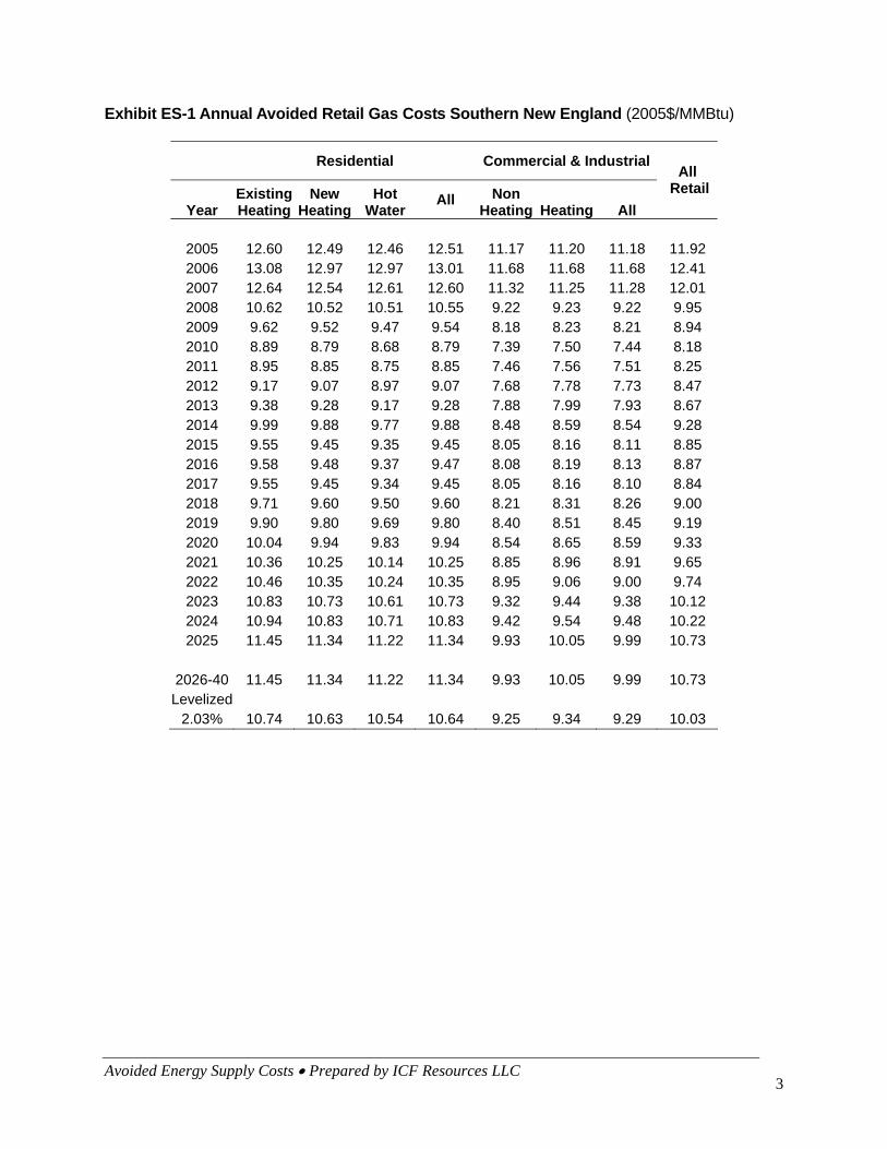
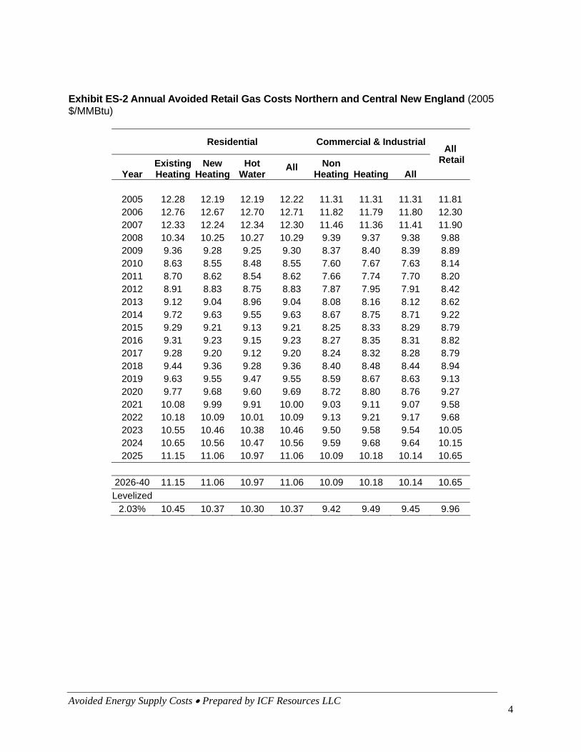
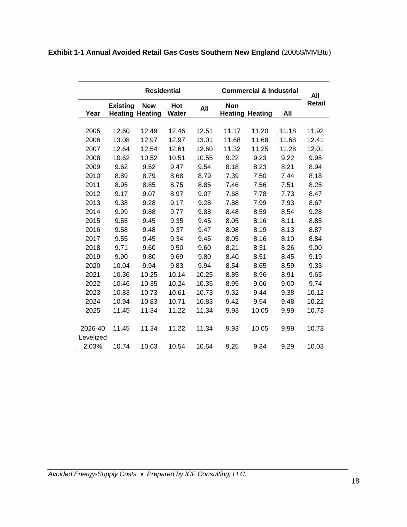
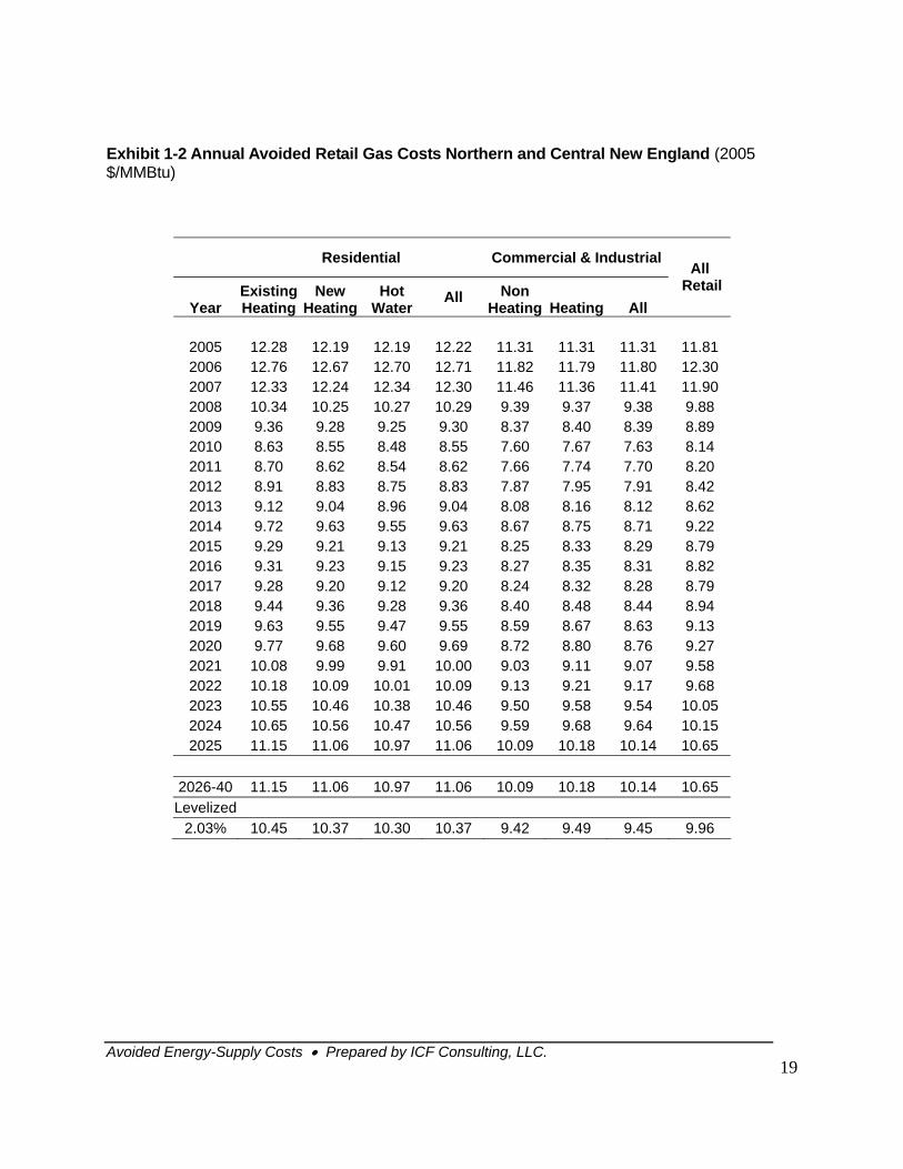
Retail avoided natural gas costs in New England are expected to decline in real terms through roughly 2015 before gradually increasing through 2025. Avoided retail gas costs are held flat thereafter. Exhibits ES-1 and ES-2 present the annual avoided retail gas costs for the residential and commercial sectors for Southern New England and Northern and Central New England.
Results for the residential sector are provided for existing heating, new heating, and hot water. Average results for all residential are also provided. Results for the commercial and industrial sector are provided are provided for non-heating and heating as well as the average for the sector.
Avoided Energy Supply Costs • Prepared by ICF Resources LLC 3
Exhibit ES-1 Annual Avoided Retail Gas Costs Southern New England (2005$/MMBtu)
Residential Commercial & Industrial
Year Existing Heating
New Heating
Hot Water
All Non Heating Heating All
All Retail
2005 12.60 12.49 12.46 12.51 11.17 11.20 11.18 11.92 2006 13.08 12.97 12.97 13.01 11.68 11.68 11.68 12.41 2007 12.64 12.54 12.61 12.60 11.32 11.25 11.28 12.01 2008 10.62 10.52 10.51 10.55 9.22 9.23 9.22 9.95 2009 9.62 9.52 9.47 9.54 8.18 8.23 8.21 8.94 2010 8.89 8.79 8.68 8.79 7.39 7.50 7.44 8.18 2011 8.95 8.85 8.75 8.85 7.46 7.56 7.51 8.25 2012 9.17 9.07 8.97 9.07 7.68 7.78 7.73 8.47 2013 9.38 9.28 9.17 9.28 7.88 7.99 7.93 8.67 2014 9.99 9.88 9.77 9.88 8.48 8.59 8.54 9.28 2015 9.55 9.45 9.35 9.45 8.05 8.16 8.11 8.85 2016 9.58 9.48 9.37 9.47 8.08 8.19 8.13 8.87 2017 9.55 9.45 9.34 9.45 8.05 8.16 8.10 8.84 2018 9.71 9.60 9.50 9.60 8.21 8.31 8.26 9.00 2019 9.90 9.80 9.69 9.80 8.40 8.51 8.45 9.19 2020 10.04 9.94 9.83 9.94 8.54 8.65 8.59 9.33 2021 10.36 10.25 10.14 10.25 8.85 8.96 8.91 9.65 2022 10.46 10.35 10.24 10.35 8.95 9.06 9.00 9.74 2023 10.83 10.73 10.61 10.73 9.32 9.44 9.38 10.12 2024 10.94 10.83 10.71 10.83 9.42 9.54 9.48 10.22 2025 11.45 11.34 11.22 11.34 9.93 10.05 9.99 10.73
2026-40 11.45 11.34 11.22 11.34 9.93 10.05 9.99 10.73 Levelized
2.03% 10.74 10.63 10.54 10.64 9.25 9.34 9.29 10.03
Avoided Energy Supply Costs • Prepared by ICF Resources LLC 4
Exhibit ES-2 Annual Avoided Retail Gas Costs Northern and Central New England (2005 $/MMBtu)
Residential Commercial & Industrial
Year Existing Heating
New Heating
Hot Water
All Non Heating Heating All
All Retail
2005 12.28 12.19 12.19 12.22 11.31 11.31 11.31 11.81 2006 12.76 12.67 12.70 12.71 11.82 11.79 11.80 12.30 2007 12.33 12.24 12.34 12.30 11.46 11.36 11.41 11.90 2008 10.34 10.25 10.27 10.29 9.39 9.37 9.38 9.88 2009 9.36 9.28 9.25 9.30 8.37 8.40 8.39 8.89 2010 8.63 8.55 8.48 8.55 7.60 7.67 7.63 8.14 2011 8.70 8.62 8.54 8.62 7.66 7.74 7.70 8.20 2012 8.91 8.83 8.75 8.83 7.87 7.95 7.91 8.42 2013 9.12 9.04 8.96 9.04 8.08 8.16 8.12 8.62 2014 9.72 9.63 9.55 9.63 8.67 8.75 8.71 9.22 2015 9.29 9.21 9.13 9.21 8.25 8.33 8.29 8.79 2016 9.31 9.23 9.15 9.23 8.27 8.35 8.31 8.82 2017 9.28 9.20 9.12 9.20 8.24 8.32 8.28 8.79 2018 9.44 9.36 9.28 9.36 8.40 8.48 8.44 8.94 2019 9.63 9.55 9.47 9.55 8.59 8.67 8.63 9.13 2020 9.77 9.68 9.60 9.69 8.72 8.80 8.76 9.27 2021 10.08 9.99 9.91 10.00 9.03 9.11 9.07 9.58 2022 10.18 10.09 10.01 10.09 9.13 9.21 9.17 9.68 2023 10.55 10.46 10.38 10.46 9.50 9.58 9.54 10.05 2024 10.65 10.56 10.47 10.56 9.59 9.68 9.64 10.15 2025 11.15 11.06 10.97 11.06 10.09 10.18 10.14 10.65
2026-40 11.15 11.06 10.97 11.06 10.09 10.18 10.14 10.65 Levelized
2.03% 10.45 10.37 10.30 10.37 9.42 9.49 9.45 9.96
Avoided Energy Supply Costs • Prepared by ICF Resources LLC 5
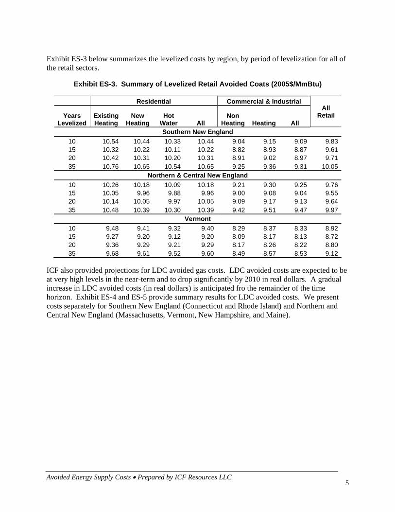
Exhibit ES-3 below summarizes the levelized costs by region, by period of levelization for all of the retail sectors.
Exhibit ES-3. Summary of Levelized Retail Avoided Coats (2005$/MmBtu)
Residential Commercial & Industrial
Years Levelized
Existing Heating
New Heating
Hot Water All
Non Heating Heating All
All Retail
Southern New England 10 10.54 10.44 10.33 10.44 9.04 9.15 9.09 9.8315 10.32 10.22 10.11 10.22 8.82 8.93 8.87 9.6120 10.42 10.31 10.20 10.31 8.91 9.02 8.97 9.7135 10.76 10.65 10.54 10.65 9.25 9.36 9.31 10.05
Northern & Central New England 10 10.26 10.18 10.09 10.18 9.21 9.30 9.25 9.7615 10.05 9.96 9.88 9.96 9.00 9.08 9.04 9.5520 10.14 10.05 9.97 10.05 9.09 9.17 9.13 9.6435 10.48 10.39 10.30 10.39 9.42 9.51 9.47 9.97
Vermont 10 9.48 9.41 9.32 9.40 8.29 8.37 8.33 8.9215 9.27 9.20 9.12 9.20 8.09 8.17 8.13 8.7220 9.36 9.29 9.21 9.29 8.17 8.26 8.22 8.8035 9.68 9.61 9.52 9.60 8.49 8.57 8.53 9.12
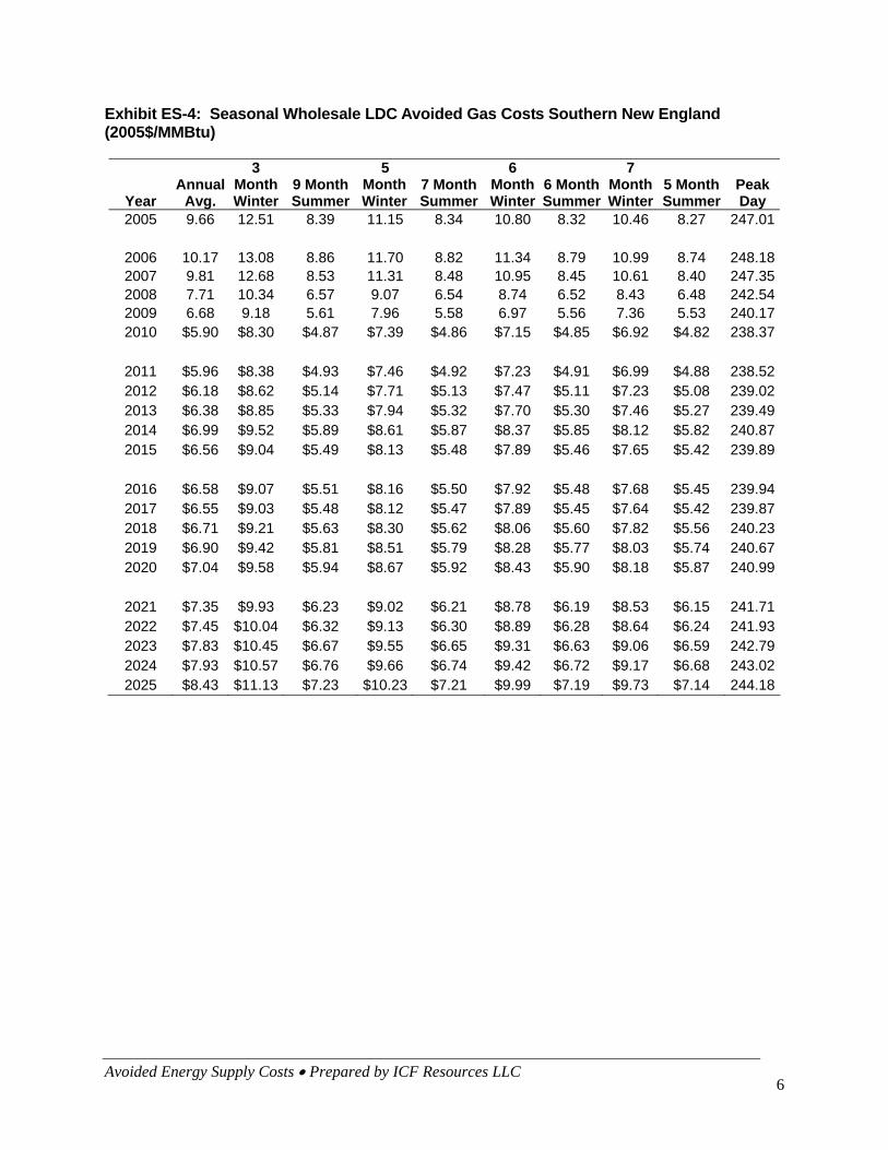
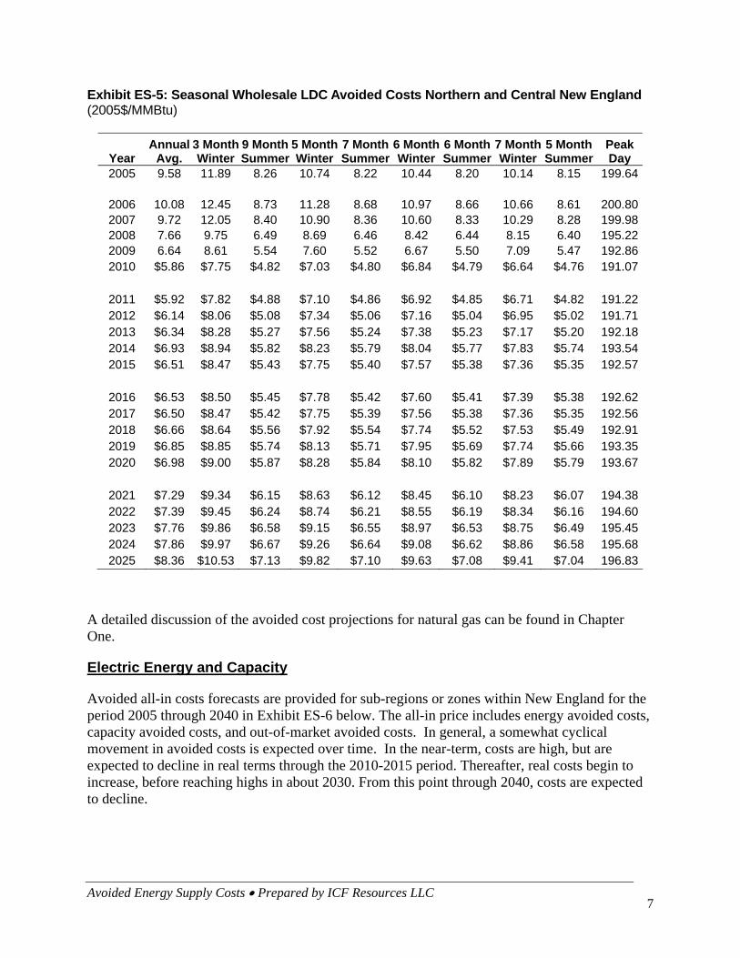
ICF also provided projections for LDC avoided gas costs. LDC avoided costs are expected to be at very high levels in the near-term and to drop significantly by 2010 in real dollars. A gradual increase in LDC avoided costs (in real dollars) is anticipated fro the remainder of the time horizon. Exhibit ES-4 and ES-5 provide summary results for LDC avoided costs. We present costs separately for Southern New England (Connecticut and Rhode Island) and Northern and Central New England (Massachusetts, Vermont, New Hampshire, and Maine).
Avoided Energy Supply Costs • Prepared by ICF Resources LLC 6
Exhibit ES-4: Seasonal Wholesale LDC Avoided Gas Costs Southern New England (2005$/MMBtu)
Year Annual
Avg.
3 Month Winter
9 Month Summer
5 Month Winter
7 Month Summer
6 Month Winter
6 Month Summer
7 Month Winter
5 Month Summer
Peak Day
2005 9.66 12.51 8.39 11.15 8.34 10.80 8.32 10.46 8.27 247.01
2006 10.17 13.08 8.86 11.70 8.82 11.34 8.79 10.99 8.74 248.182007 9.81 12.68 8.53 11.31 8.48 10.95 8.45 10.61 8.40 247.352008 7.71 10.34 6.57 9.07 6.54 8.74 6.52 8.43 6.48 242.542009 6.68 9.18 5.61 7.96 5.58 6.97 5.56 7.36 5.53 240.172010 $5.90 $8.30 $4.87 $7.39 $4.86 $7.15 $4.85 $6.92 $4.82 238.37
2011 $5.96 $8.38 $4.93 $7.46 $4.92 $7.23 $4.91 $6.99 $4.88 238.522012 $6.18 $8.62 $5.14 $7.71 $5.13 $7.47 $5.11 $7.23 $5.08 239.022013 $6.38 $8.85 $5.33 $7.94 $5.32 $7.70 $5.30 $7.46 $5.27 239.492014 $6.99 $9.52 $5.89 $8.61 $5.87 $8.37 $5.85 $8.12 $5.82 240.872015 $6.56 $9.04 $5.49 $8.13 $5.48 $7.89 $5.46 $7.65 $5.42 239.89
2016 $6.58 $9.07 $5.51 $8.16 $5.50 $7.92 $5.48 $7.68 $5.45 239.942017 $6.55 $9.03 $5.48 $8.12 $5.47 $7.89 $5.45 $7.64 $5.42 239.872018 $6.71 $9.21 $5.63 $8.30 $5.62 $8.06 $5.60 $7.82 $5.56 240.232019 $6.90 $9.42 $5.81 $8.51 $5.79 $8.28 $5.77 $8.03 $5.74 240.672020 $7.04 $9.58 $5.94 $8.67 $5.92 $8.43 $5.90 $8.18 $5.87 240.99
2021 $7.35 $9.93 $6.23 $9.02 $6.21 $8.78 $6.19 $8.53 $6.15 241.712022 $7.45 $10.04 $6.32 $9.13 $6.30 $8.89 $6.28 $8.64 $6.24 241.932023 $7.83 $10.45 $6.67 $9.55 $6.65 $9.31 $6.63 $9.06 $6.59 242.792024 $7.93 $10.57 $6.76 $9.66 $6.74 $9.42 $6.72 $9.17 $6.68 243.022025 $8.43 $11.13 $7.23 $10.23 $7.21 $9.99 $7.19 $9.73 $7.14 244.18
Avoided Energy Supply Costs • Prepared by ICF Resources LLC 7
Exhibit ES-5: Seasonal Wholesale LDC Avoided Costs Northern and Central New England (2005$/MMBtu)
Year Annual
Avg. 3 Month Winter
9 Month Summer
5 MonthWinter
7 Month Summer
6 Month Winter
6 Month Summer
7 Month Winter
5 Month Summer
Peak Day
2005 9.58 11.89 8.26 10.74 8.22 10.44 8.20 10.14 8.15 199.64
2006 10.08 12.45 8.73 11.28 8.68 10.97 8.66 10.66 8.61 200.802007 9.72 12.05 8.40 10.90 8.36 10.60 8.33 10.29 8.28 199.982008 7.66 9.75 6.49 8.69 6.46 8.42 6.44 8.15 6.40 195.222009 6.64 8.61 5.54 7.60 5.52 6.67 5.50 7.09 5.47 192.862010 $5.86 $7.75 $4.82 $7.03 $4.80 $6.84 $4.79 $6.64 $4.76 191.07
2011 $5.92 $7.82 $4.88 $7.10 $4.86 $6.92 $4.85 $6.71 $4.82 191.222012 $6.14 $8.06 $5.08 $7.34 $5.06 $7.16 $5.04 $6.95 $5.02 191.712013 $6.34 $8.28 $5.27 $7.56 $5.24 $7.38 $5.23 $7.17 $5.20 192.182014 $6.93 $8.94 $5.82 $8.23 $5.79 $8.04 $5.77 $7.83 $5.74 193.542015 $6.51 $8.47 $5.43 $7.75 $5.40 $7.57 $5.38 $7.36 $5.35 192.57
2016 $6.53 $8.50 $5.45 $7.78 $5.42 $7.60 $5.41 $7.39 $5.38 192.622017 $6.50 $8.47 $5.42 $7.75 $5.39 $7.56 $5.38 $7.36 $5.35 192.562018 $6.66 $8.64 $5.56 $7.92 $5.54 $7.74 $5.52 $7.53 $5.49 192.912019 $6.85 $8.85 $5.74 $8.13 $5.71 $7.95 $5.69 $7.74 $5.66 193.352020 $6.98 $9.00 $5.87 $8.28 $5.84 $8.10 $5.82 $7.89 $5.79 193.67
2021 $7.29 $9.34 $6.15 $8.63 $6.12 $8.45 $6.10 $8.23 $6.07 194.382022 $7.39 $9.45 $6.24 $8.74 $6.21 $8.55 $6.19 $8.34 $6.16 194.602023 $7.76 $9.86 $6.58 $9.15 $6.55 $8.97 $6.53 $8.75 $6.49 195.452024 $7.86 $9.97 $6.67 $9.26 $6.64 $9.08 $6.62 $8.86 $6.58 195.682025 $8.36 $10.53 $7.13 $9.82 $7.10 $9.63 $7.08 $9.41 $7.04 196.83
A detailed discussion of the avoided cost projections for natural gas can be found in Chapter One.
Electric Energy and Capacity
Avoided all-in costs forecasts are provided for sub-regions or zones within New England for the period 2005 through 2040 in Exhibit ES-6 below. The all-in price includes energy avoided costs, capacity avoided costs, and out-of-market avoided costs. In general, a somewhat cyclical movement in avoided costs is expected over time. In the near-term, costs are high, but are expected to decline in real terms through the 2010-2015 period. Thereafter, real costs begin to increase, before reaching highs in about 2030. From this point through 2040, costs are expected to decline.
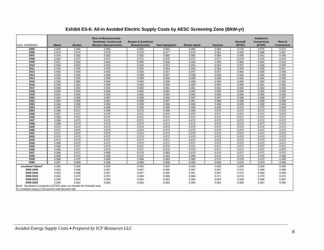
Exhibit ES-6: All-in Avoided Electric Supply Costs by AESC Screening Zone ($/kW-yr)
Units :2005$/kWh Maine Boston
Rest of Massachusetts - Southeast, Central and Western Massachusetts
Boston & Southeast Massachusetts New Hampshire Rhode Island Vermont
Norwalk (RTEP)
Southwest Connecticut
(RTEP)Rest of
Connecticut 2005 0.063 0.066 0.066 0.066 0.064 0.066 0.068 0.076 0.075 0.0722006 0.074 0.079 0.079 0.079 0.077 0.079 0.081 0.093 0.088 0.0872007 0.076 0.082 0.082 0.082 0.080 0.082 0.084 0.095 0.091 0.0902008 0.063 0.072 0.072 0.072 0.070 0.072 0.073 0.078 0.076 0.0752009 0.051 0.060 0.060 0.060 0.058 0.060 0.060 0.065 0.064 0.0622010 0.046 0.053 0.053 0.053 0.052 0.053 0.054 0.057 0.056 0.0552011 0.050 0.056 0.055 0.055 0.054 0.055 0.055 0.059 0.058 0.0572012 0.055 0.058 0.058 0.058 0.057 0.057 0.057 0.060 0.059 0.0582013 0.055 0.059 0.058 0.058 0.057 0.058 0.058 0.060 0.060 0.0592014 0.055 0.059 0.059 0.059 0.058 0.058 0.058 0.060 0.060 0.0592015 0.056 0.060 0.059 0.060 0.058 0.059 0.059 0.060 0.060 0.0592016 0.056 0.061 0.059 0.060 0.059 0.059 0.060 0.060 0.061 0.0602017 0.058 0.062 0.061 0.062 0.061 0.061 0.061 0.062 0.062 0.0622018 0.059 0.064 0.063 0.064 0.062 0.063 0.063 0.064 0.064 0.0632019 0.061 0.066 0.065 0.066 0.064 0.065 0.065 0.066 0.066 0.0652020 0.063 0.068 0.067 0.068 0.066 0.067 0.067 0.068 0.068 0.0672021 0.064 0.069 0.067 0.068 0.067 0.067 0.068 0.068 0.068 0.0682022 0.064 0.069 0.068 0.069 0.068 0.068 0.068 0.069 0.069 0.0682023 0.065 0.070 0.069 0.069 0.068 0.069 0.069 0.070 0.070 0.0692024 0.066 0.071 0.069 0.070 0.069 0.069 0.070 0.070 0.070 0.0702025 0.067 0.071 0.070 0.071 0.070 0.070 0.071 0.071 0.071 0.0702026 0.068 0.072 0.071 0.071 0.070 0.071 0.071 0.071 0.072 0.0712027 0.069 0.073 0.071 0.072 0.071 0.072 0.072 0.072 0.072 0.0722028 0.069 0.073 0.072 0.073 0.072 0.072 0.073 0.073 0.073 0.0722029 0.070 0.074 0.073 0.074 0.073 0.073 0.074 0.073 0.074 0.0732030 0.071 0.075 0.073 0.074 0.073 0.074 0.074 0.074 0.074 0.0742031 0.071 0.074 0.073 0.074 0.073 0.073 0.074 0.074 0.074 0.0732032 0.070 0.073 0.072 0.073 0.072 0.073 0.073 0.073 0.073 0.0722033 0.070 0.073 0.071 0.072 0.071 0.072 0.073 0.072 0.072 0.0722034 0.069 0.072 0.071 0.072 0.071 0.071 0.072 0.072 0.072 0.0712035 0.069 0.072 0.070 0.071 0.070 0.071 0.071 0.072 0.072 0.0712036 0.068 0.071 0.070 0.071 0.070 0.070 0.071 0.071 0.071 0.0702037 0.068 0.071 0.069 0.070 0.069 0.070 0.070 0.071 0.071 0.0702038 0.068 0.070 0.069 0.070 0.069 0.069 0.070 0.071 0.070 0.0692039 0.068 0.070 0.069 0.069 0.069 0.069 0.070 0.070 0.070 0.0692040 0.067 0.069 0.068 0.069 0.068 0.069 0.069 0.070 0.070 0.069
Levelized Values1 0.000 0.000 0.000 0.000 0.000 0.000 0.000 0.000 0.000 0.0002005-2040 0.063 0.068 0.067 0.067 0.066 0.067 0.067 0.070 0.069 0.0682006-2040 0.063 0.068 0.067 0.067 0.066 0.067 0.067 0.070 0.069 0.0682006-2010 0.062 0.070 0.070 0.069 0.068 0.069 0.071 0.078 0.075 0.0742006-2015 0.058 0.064 0.064 0.064 0.063 0.064 0.064 0.069 0.068 0.0672006-2020 0.059 0.064 0.064 0.064 0.063 0.063 0.064 0.068 0.067 0.066
Note: Southwest Connecticut (RTEP) does not include the Norwalk area.1) Levelized using a 2.03 percent real discount rate
Avoided Energy Supply Costs • Prepared by ICF Resources LLC 8
Avoided Energy Supply Costs • Prepared by ICF Resources LLC 9
Background on the methodology and assumptions used to derive the electric avoided costs can be found in Chapter Two. Further detail on the electric energy avoided cost results, including a breakout of the component costs can be found in Chapter Three and Appendix Two. The material presented in these chapters is presented for separate costing periods as described in Appendix One.
Other Fuels
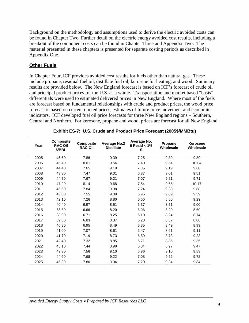
In Chapter Four, ICF provides avoided cost results for fuels other than natural gas. These include propane, residual fuel oil, distillate fuel oil, kerosene for heating, and wood. Summary results are provided below. The New England forecast is based on ICF’s forecast of crude oil and principal product prices for the U.S. as a whole. Transportation and market based “basis” differentials were used to estimated delivered prices in New England. Where most of the fuels are forecast based on fundamental relationships with crude and product prices, the wood price forecast is based on current quoted prices, estimates of future price movement and economic indicators. ICF developed fuel oil price forecasts for three New England regions – Southern, Central and Northern. For kerosene, propane and wood, prices are forecast for all New England.
Exhibit ES-7: U.S. Crude and Product Price Forecast (2005$/MMBtu)
Year Composite
RAC Oil $/BBL
Composite RAC Oil
Average No.2 Distillate
Average No. 6 Resid < 1%
S Propane
Wholesale Kerosene Wholesale
2005 45.60 7.86 9.39 7.25 9.39 9.89 2006 46.40 8.01 9.54 7.40 9.54 10.04 2007 44.40 7.65 9.19 7.05 9.19 9.68 2008 43.30 7.47 9.01 6.87 9.01 9.51 2009 44.50 7.67 9.21 7.07 9.21 9.71 2010 47.20 8.14 9.68 7.54 9.68 10.17 2011 45.50 7.84 9.38 7.24 9.38 9.88 2012 43.80 7.55 9.09 6.95 9.09 9.59 2013 42.10 7.26 8.80 6.66 8.80 9.29 2014 40.40 6.97 8.51 6.37 8.51 9.00 2015 38.60 6.66 8.20 6.06 8.20 8.69 2016 38.90 6.71 8.25 6.10 8.24 8.74 2017 39.60 6.83 8.37 6.23 8.37 8.86 2018 40.30 6.95 8.49 6.35 8.49 8.99 2019 41.00 7.07 8.61 6.47 8.61 9.11 2020 41.70 7.19 8.73 6.59 8.73 9.23 2021 42.40 7.32 8.85 6.71 8.85 9.35 2022 43.10 7.44 8.98 6.84 8.97 9.47 2023 43.80 7.56 9.10 6.96 9.10 9.59 2024 44.60 7.68 9.22 7.08 9.22 9.72 2025 45.30 7.80 9.34 7.20 9.34 9.84
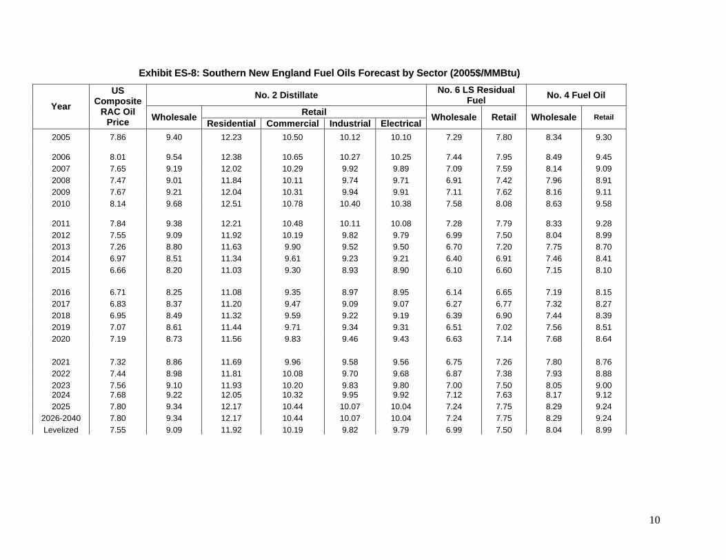
Exhibit ES-8: Southern New England Fuel Oils Forecast by Sector (2005$/MMBtu)
No. 2 Distillate No. 6 LS Residual Fuel No. 4 Fuel Oil
Retail Year US
Composite RAC Oil
Price Wholesale Residential Commercial Industrial Electrical Wholesale Retail Wholesale Retail
2005 7.86 9.40 12.23 10.50 10.12 10.10 7.29 7.80 8.34 9.30
2006 8.01 9.54 12.38 10.65 10.27 10.25 7.44 7.95 8.49 9.452007 7.65 9.19 12.02 10.29 9.92 9.89 7.09 7.59 8.14 9.092008 7.47 9.01 11.84 10.11 9.74 9.71 6.91 7.42 7.96 8.912009 7.67 9.21 12.04 10.31 9.94 9.91 7.11 7.62 8.16 9.112010 8.14 9.68 12.51 10.78 10.40 10.38 7.58 8.08 8.63 9.58
2011 7.84 9.38 12.21 10.48 10.11 10.08 7.28 7.79 8.33 9.282012 7.55 9.09 11.92 10.19 9.82 9.79 6.99 7.50 8.04 8.992013 7.26 8.80 11.63 9.90 9.52 9.50 6.70 7.20 7.75 8.702014 6.97 8.51 11.34 9.61 9.23 9.21 6.40 6.91 7.46 8.412015 6.66 8.20 11.03 9.30 8.93 8.90 6.10 6.60 7.15 8.10
2016 6.71 8.25 11.08 9.35 8.97 8.95 6.14 6.65 7.19 8.152017 6.83 8.37 11.20 9.47 9.09 9.07 6.27 6.77 7.32 8.272018 6.95 8.49 11.32 9.59 9.22 9.19 6.39 6.90 7.44 8.392019 7.07 8.61 11.44 9.71 9.34 9.31 6.51 7.02 7.56 8.512020 7.19 8.73 11.56 9.83 9.46 9.43 6.63 7.14 7.68 8.64
2021 7.32 8.86 11.69 9.96 9.58 9.56 6.75 7.26 7.80 8.762022 7.44 8.98 11.81 10.08 9.70 9.68 6.87 7.38 7.93 8.882023 7.56 9.10 11.93 10.20 9.83 9.80 7.00 7.50 8.05 9.002024 7.68 9.22 12.05 10.32 9.95 9.92 7.12 7.63 8.17 9.122025 7.80 9.34 12.17 10.44 10.07 10.04 7.24 7.75 8.29 9.24
2026-2040 7.80 9.34 12.17 10.44 10.07 10.04 7.24 7.75 8.29 9.24Levelized 7.55 9.09 11.92 10.19 9.82 9.79 6.99 7.50 8.04 8.99
10

Exhibit ES-9: Northern New England Fuel Oils Forecast by Sector (2005$/MMBtu)
No. 2 Distillate No. 6 Residual Fuel <= 1% Sulfur No. 4 Fuel Oil
Retail Year
CrudeWholesale Residential Commercial Industrial Electrical Wholesale Retail Wholesale Retail
2005 7.86 9.46 12.22 10.35 10.45 10.85 7.29 7.80 8.38 9.43
2006 8.01 9.61 12.37 10.50 10.60 11.00 7.44 7.95 8.52 9.582007 7.65 9.25 12.02 10.14 10.24 10.65 7.09 7.59 8.17 9.222008 7.47 9.07 11.84 9.97 10.06 10.47 6.91 7.42 7.99 9.042009 7.67 9.27 12.04 10.17 10.26 10.67 7.11 7.62 8.19 9.242010 8.14 9.74 12.51 10.63 10.73 11.13 7.58 8.08 8.66 9.71
2011 7.84 9.44 12.21 10.34 10.43 10.84 7.28 7.79 8.36 9.412012 7.55 9.15 11.92 10.04 10.14 10.55 6.99 7.50 8.07 9.122013 7.26 8.86 11.63 9.75 9.85 10.25 6.70 7.20 7.78 8.832014 6.97 8.57 11.34 9.46 9.56 9.96 6.40 6.91 7.49 8.542015 6.66 8.26 11.03 9.15 9.25 9.66 6.10 6.60 7.18 8.23
2016 6.71 8.31 11.07 9.20 9.30 9.70 6.14 6.65 7.23 8.282017 6.83 8.43 11.20 9.32 9.42 9.82 6.27 6.77 7.35 8.402018 6.95 8.55 11.32 9.45 9.54 9.95 6.39 6.90 7.47 8.522019 7.07 8.67 11.44 9.57 9.66 10.07 6.51 7.02 7.59 8.642020 7.19 8.80 11.56 9.69 9.78 10.19 6.63 7.14 7.71 8.76
2021 7.32 8.92 11.68 9.81 9.91 10.31 6.75 7.26 7.84 8.892022 7.44 9.04 11.81 9.93 10.03 10.43 6.87 7.38 7.96 9.012023 7.56 9.16 11.93 10.05 10.15 10.56 7.00 7.50 8.08 9.132024 7.68 9.28 12.05 10.18 10.27 10.68 7.12 7.63 8.20 9.252025 7.80 9.40 12.17 10.30 10.39 10.80 7.24 7.75 8.32 9.37
2026-2040 7.80 9.40 12.17 10.30 10.39 10.80 7.24 7.75 8.32 9.37Levelized 7.55 9.15 11.92 10.05 10.14 10.55 6.99 7.50 8.07 9.12
11
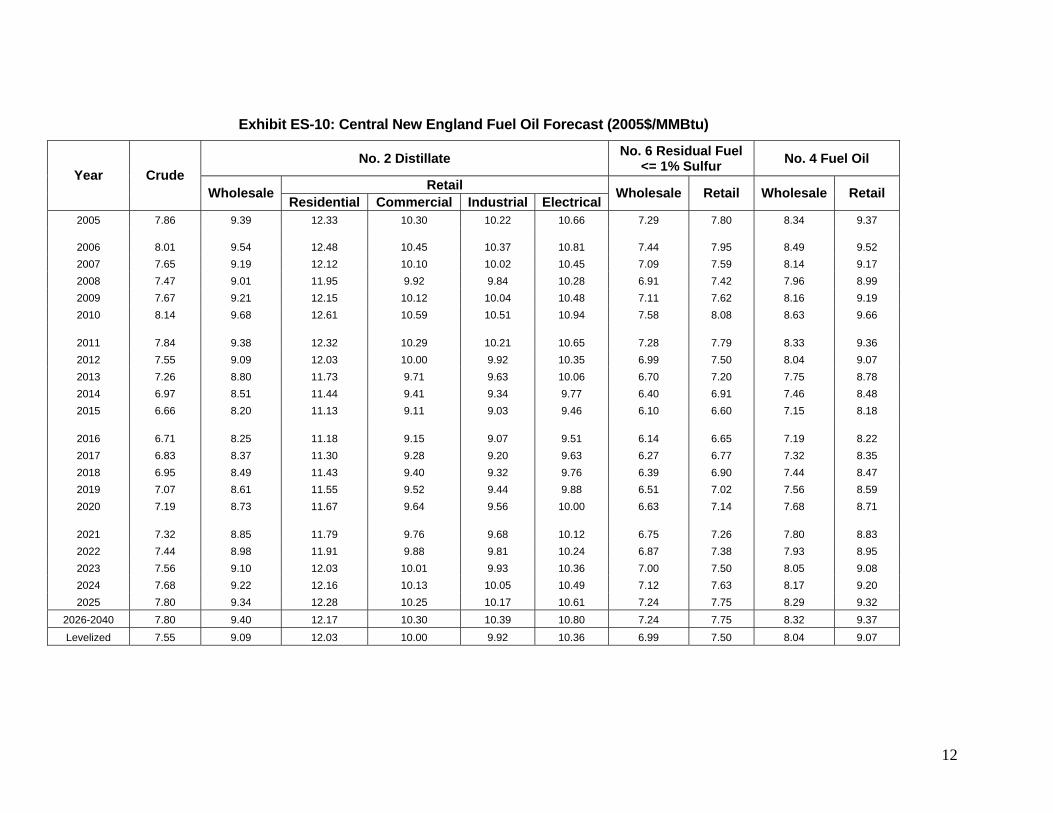
Exhibit ES-10: Central New England Fuel Oil Forecast (2005$/MMBtu)
No. 2 Distillate No. 6 Residual Fuel <= 1% Sulfur No. 4 Fuel Oil
Retail Year
Crude
Wholesale Residential Commercial Industrial Electrical Wholesale Retail Wholesale Retail
2005 7.86 9.39 12.33 10.30 10.22 10.66 7.29 7.80 8.34 9.37
2006 8.01 9.54 12.48 10.45 10.37 10.81 7.44 7.95 8.49 9.522007 7.65 9.19 12.12 10.10 10.02 10.45 7.09 7.59 8.14 9.172008 7.47 9.01 11.95 9.92 9.84 10.28 6.91 7.42 7.96 8.992009 7.67 9.21 12.15 10.12 10.04 10.48 7.11 7.62 8.16 9.192010 8.14 9.68 12.61 10.59 10.51 10.94 7.58 8.08 8.63 9.66
2011 7.84 9.38 12.32 10.29 10.21 10.65 7.28 7.79 8.33 9.362012 7.55 9.09 12.03 10.00 9.92 10.35 6.99 7.50 8.04 9.072013 7.26 8.80 11.73 9.71 9.63 10.06 6.70 7.20 7.75 8.782014 6.97 8.51 11.44 9.41 9.34 9.77 6.40 6.91 7.46 8.482015 6.66 8.20 11.13 9.11 9.03 9.46 6.10 6.60 7.15 8.18
2016 6.71 8.25 11.18 9.15 9.07 9.51 6.14 6.65 7.19 8.222017 6.83 8.37 11.30 9.28 9.20 9.63 6.27 6.77 7.32 8.352018 6.95 8.49 11.43 9.40 9.32 9.76 6.39 6.90 7.44 8.472019 7.07 8.61 11.55 9.52 9.44 9.88 6.51 7.02 7.56 8.592020 7.19 8.73 11.67 9.64 9.56 10.00 6.63 7.14 7.68 8.71
2021 7.32 8.85 11.79 9.76 9.68 10.12 6.75 7.26 7.80 8.832022 7.44 8.98 11.91 9.88 9.81 10.24 6.87 7.38 7.93 8.952023 7.56 9.10 12.03 10.01 9.93 10.36 7.00 7.50 8.05 9.082024 7.68 9.22 12.16 10.13 10.05 10.49 7.12 7.63 8.17 9.202025 7.80 9.34 12.28 10.25 10.17 10.61 7.24 7.75 8.29 9.32
2026-2040 7.80 9.40 12.17 10.30 10.39 10.80 7.24 7.75 8.32 9.37Levelized 7.55 9.09 12.03 10.00 9.92 10.36 6.99 7.50 8.04 9.07
12
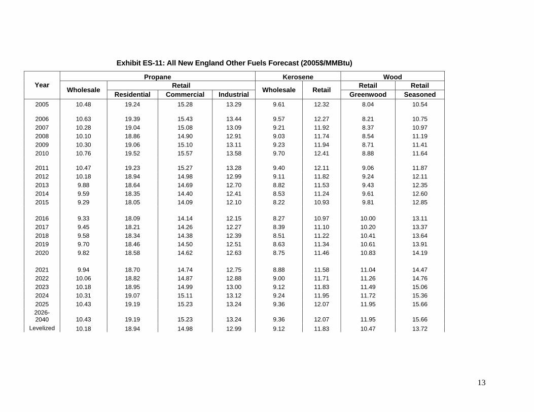
Exhibit ES-11: All New England Other Fuels Forecast (2005$/MMBtu)
Propane Kerosene WoodRetail Retail RetailYear
Wholesale Residential Commercial Industrial Wholesale Retail Greenwood Seasoned2005 10.48 19.24 15.28 13.29 9.61 12.32 8.04 10.54
2006 10.63 19.39 15.43 13.44 9.57 12.27 8.21 10.752007 10.28 19.04 15.08 13.09 9.21 11.92 8.37 10.972008 10.10 18.86 14.90 12.91 9.03 11.74 8.54 11.192009 10.30 19.06 15.10 13.11 9.23 11.94 8.71 11.412010 10.76 19.52 15.57 13.58 9.70 12.41 8.88 11.64
2011 10.47 19.23 15.27 13.28 9.40 12.11 9.06 11.872012 10.18 18.94 14.98 12.99 9.11 11.82 9.24 12.112013 9.88 18.64 14.69 12.70 8.82 11.53 9.43 12.352014 9.59 18.35 14.40 12.41 8.53 11.24 9.61 12.602015 9.29 18.05 14.09 12.10 8.22 10.93 9.81 12.85
2016 9.33 18.09 14.14 12.15 8.27 10.97 10.00 13.112017 9.45 18.21 14.26 12.27 8.39 11.10 10.20 13.372018 9.58 18.34 14.38 12.39 8.51 11.22 10.41 13.642019 9.70 18.46 14.50 12.51 8.63 11.34 10.61 13.912020 9.82 18.58 14.62 12.63 8.75 11.46 10.83 14.19
2021 9.94 18.70 14.74 12.75 8.88 11.58 11.04 14.472022 10.06 18.82 14.87 12.88 9.00 11.71 11.26 14.762023 10.18 18.95 14.99 13.00 9.12 11.83 11.49 15.062024 10.31 19.07 15.11 13.12 9.24 11.95 11.72 15.362025 10.43 19.19 15.23 13.24 9.36 12.07 11.95 15.662026-2040 10.43 19.19 15.23 13.24 9.36 12.07 11.95 15.66
Levelized 10.18 18.94 14.98 12.99 9.12 11.83 10.47 13.72
13
Avoided Energy Supply Costs • Prepared by ICF Resources LLC 14
Transmission and Distribution Capacity
ICF was asked to recommend a methodological approach which could be used by AESC study group participants to project avoided transmission and distribution capacity costs. The recommendation was intended to be designed to be able to be used by all participants individually. In order to accommodate this, ICF interviewed many of the participants to understand their current methodology and the data available to them. Based on this, ICF provided a recommended approach, and a spreadsheet tool which could be used to implement this approach, to the study group. The recommendation and tool are discussed in Chapter Five.
Demand Reduction Induced Price Effects
In addition to the core electric avoided costs described above, ICF was asked to determine if additional benefits may result from price response to demand reductions. Demand reduction induced price effects (DRIPE) reflect any change in addition to the avoided costs that occur due to a price response that results from the demand reduction. Exhibit ES-12 presents the results of the DRIPE analysis. A DRIPE Light scenario was also considered and is presented in Exhibit ES-13. Discussion of the DRIPE analysis and results is found in Chapter Six.
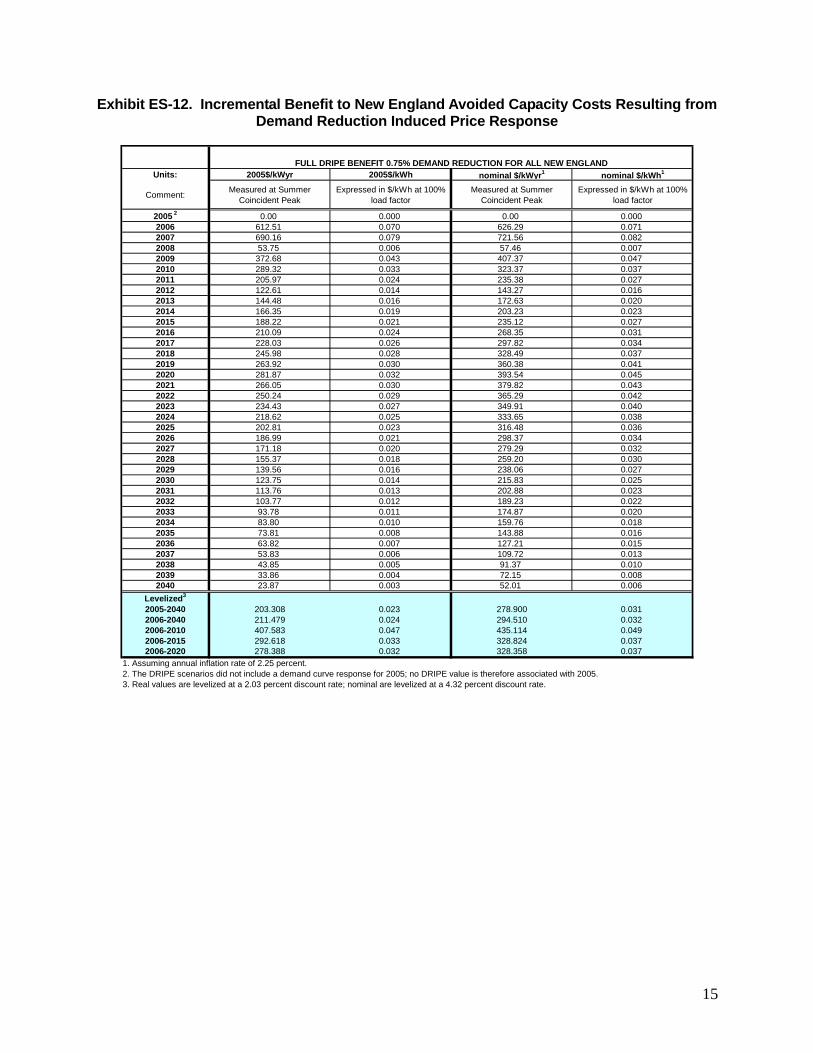
Exhibit ES-12. Incremental Benefit to New England Avoided Capacity Costs Resulting from Demand Reduction Induced Price Response
Units: 2005$/kWyr 2005$/kWh nominal $/kWyr1 nominal $/kWh1
Comment: Measured at Summer Coincident Peak
Expressed in $/kWh at 100% load factor
Measured at Summer Coincident Peak
Expressed in $/kWh at 100% load factor
2005 2 0.00 0.000 0.00 0.0002006 612.51 0.070 626.29 0.0712007 690.16 0.079 721.56 0.0822008 53.75 0.006 57.46 0.0072009 372.68 0.043 407.37 0.0472010 289.32 0.033 323.37 0.0372011 205.97 0.024 235.38 0.0272012 122.61 0.014 143.27 0.0162013 144.48 0.016 172.63 0.0202014 166.35 0.019 203.23 0.0232015 188.22 0.021 235.12 0.0272016 210.09 0.024 268.35 0.0312017 228.03 0.026 297.82 0.0342018 245.98 0.028 328.49 0.0372019 263.92 0.030 360.38 0.0412020 281.87 0.032 393.54 0.0452021 266.05 0.030 379.82 0.0432022 250.24 0.029 365.29 0.0422023 234.43 0.027 349.91 0.0402024 218.62 0.025 333.65 0.0382025 202.81 0.023 316.48 0.0362026 186.99 0.021 298.37 0.0342027 171.18 0.020 279.29 0.0322028 155.37 0.018 259.20 0.0302029 139.56 0.016 238.06 0.0272030 123.75 0.014 215.83 0.0252031 113.76 0.013 202.88 0.0232032 103.77 0.012 189.23 0.0222033 93.78 0.011 174.87 0.0202034 83.80 0.010 159.76 0.0182035 73.81 0.008 143.88 0.0162036 63.82 0.007 127.21 0.0152037 53.83 0.006 109.72 0.0132038 43.85 0.005 91.37 0.0102039 33.86 0.004 72.15 0.0082040 23.87 0.003 52.01 0.006
Levelized3
2005-2040 203.308 0.023 278.900 0.0312006-2040 211.479 0.024 294.510 0.0322006-2010 407.583 0.047 435.114 0.0492006-2015 292.618 0.033 328.824 0.0372006-2020 278.388 0.032 328.358 0.037
1. Assuming annual inflation rate of 2.25 percent.2. The DRIPE scenarios did not include a demand curve response for 2005; no DRIPE value is therefore associated with 2005.3. Real values are levelized at a 2.03 percent discount rate; nominal are levelized at a 4.32 percent discount rate.
FULL DRIPE BENEFIT 0.75% DEMAND REDUCTION FOR ALL NEW ENGLAND
15
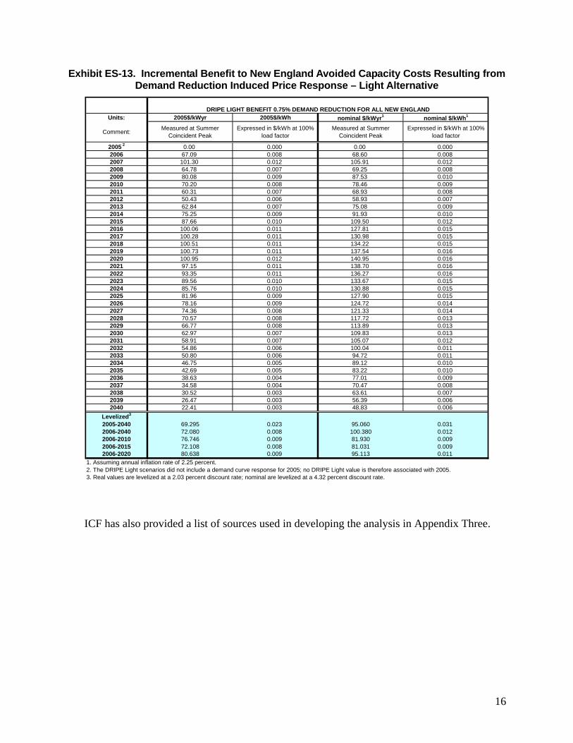
Exhibit ES-13. Incremental Benefit to New England Avoided Capacity Costs Resulting from Demand Reduction Induced Price Response – Light Alternative
Units: 2005$/kWyr 2005$/kWh nominal $/kWyr1 nominal $/kWh1
Comment: Measured at Summer Coincident Peak
Expressed in $/kWh at 100% load factor
Measured at Summer Coincident Peak
Expressed in $/kWh at 100% load factor
16
2005 2 0.00 0.000 0.00 0.0002006 67.09 0.008 68.60 0.0082007 101.30 0.012 105.91 0.0122008 64.78 0.007 69.25 0.0082009 80.08 0.009 87.53 0.0102010 70.20 0.008 78.46 0.0092011 60.31 0.007 68.93 0.0082012 50.43 0.006 58.93 0.0072013 62.84 0.007 75.08 0.0092014 75.25 0.009 91.93 0.0102015 87.66 0.010 109.50 0.0122016 100.06 0.011 127.81 0.0152017 100.28 0.011 130.98 0.0152018 100.51 0.011 134.22 0.0152019 100.73 0.011 137.54 0.0162020 100.95 0.012 140.95 0.0162021 97.15 0.011 138.70 0.0162022 93.35 0.011 136.27 0.0162023 89.56 0.010 133.67 0.0152024 85.76 0.010 130.88 0.0152025 81.96 0.009 127.90 0.0152026 78.16 0.009 124.72 0.0142027 74.36 0.008 121.33 0.0142028 70.57 0.008 117.72 0.0132029 66.77 0.008 113.89 0.0132030 62.97 0.007 109.83 0.0132031 58.91 0.007 105.07 0.0122032 54.86 0.006 100.04 0.0112033 50.80 0.006 94.72 0.0112034 46.75 0.005 89.12 0.0102035 42.69 0.005 83.22 0.0102036 38.63 0.004 77.01 0.0092037 34.58 0.004 70.47 0.0082038 30.52 0.003 63.61 0.0072039 26.47 0.003 56.39 0.0062040 22.41 0.003 48.83 0.006
Levelized3
2005-2040 69.295 0.023 95.060 0.0312006-2040 72.080 0.008 100.380 0.0122006-2010 76.746 0.009 81.930 0.0092006-2015 72.108 0.008 81.031 0.0092006-2020 80.638 0.009 95.113 0.011
1. Assuming annual inflation rate of 2.25 percent.2. The DRIPE Light scenarios did not include a demand curve response for 2005; no DRIPE Light value is therefore associated with 2005.3. Real values are levelized at a 2.03 percent discount rate; nominal are levelized at a 4.32 percent discount rate.
DRIPE LIGHT BENEFIT 0.75% EMAND REDUCTION FOR ALL NEW ENGLAND D
ICF has also provided a list of sources used in developing the analysis in Appendix Three.
17
Chapter One: Avoided Gas Costs This chapter presents the analysis of avoided gas costs. First we summarize the retail avoided gas costs for New England. Then we provide an overview of the New England gas market. The third section discusses the avoided cost methodology and the build up of the avoided cost estimates. The avoided costs by winter type and local distribution company avoided costs are in the third section. We then compare this with the previous avoided cost study. In the Appendices are found additional supporting calculations of avoided costs.
In the course of preparing this forecast, Hurricane Katrina struck the Gulf Coast and severely damaged natural gas production infrastructure. Natural gas prices soared. The forecast below takes into account the price impacts of Katrina, which are reflected in the early forecast years 2005 to 2009.
Summary of Avoided Gas Costs
Avoided natural gas costs are made up of two components, those costs avoidable by the local distribution companies (LDC) and the retail or end user avoided cost. The avoided gas costs of a LDC consist of the cost of the gas itself as well as the non-gas costs of transportation, storage and peak shaving. The avoided costs for end users also include the avoidable costs of distribution. The costs of serving a gas load vary depending on the season. Since all northern pipeline systems are designed to meet winter peak demand, avoided costs are higher in winter than in the summer. That is, a unit of gas saved in the winter allows LDCs to avoid the costs of pipe, storage, and peaking supply. In summer the avoided cost of gas service are limited to the cost of gas and the variable transportation and redelivery cost.
Below, we present a summary of our estimated avoided end user costs separately for Southern New England (Connecticut and Rhode Island) and Northern and Central New England (Massachusetts, New Hampshire, Maine). (Vermont costs are treated separately at the end of this chapter.) In the following sections, we provide an overview of the New England gas market and a description with supporting calculations of how these avoided gas cost estimates were built up. A comparison of the 2005 avoided cost calculations with the 2003 avoided cost calculations is also provided. ICF was asked to provide a separate calculation of avoided costs for Vermont given the limited market for gas in the state and the isolation from other states; a discussion of the approach used to capture the avoided costs in Vermont and the projections are included. Finally, we close with a discussion of the gas price forecasts as applied to the power sector modeling.
Avoided Energy-Supply Costs • Prepared by ICF Consulting, LLC.
18
Exhibit 1-1 Annual Avoided Retail Gas Costs Southern New England (2005$/MMBtu)
Residential Commercial & Industrial
Year Existing Heating
New Heating
Hot Water
All Non Heating Heating All
All Retail
2005 12.60 12.49 12.46 12.51 11.17 11.20 11.18 11.92 2006 13.08 12.97 12.97 13.01 11.68 11.68 11.68 12.41 2007 12.64 12.54 12.61 12.60 11.32 11.25 11.28 12.01 2008 10.62 10.52 10.51 10.55 9.22 9.23 9.22 9.95 2009 9.62 9.52 9.47 9.54 8.18 8.23 8.21 8.94 2010 8.89 8.79 8.68 8.79 7.39 7.50 7.44 8.18 2011 8.95 8.85 8.75 8.85 7.46 7.56 7.51 8.25 2012 9.17 9.07 8.97 9.07 7.68 7.78 7.73 8.47 2013 9.38 9.28 9.17 9.28 7.88 7.99 7.93 8.67 2014 9.99 9.88 9.77 9.88 8.48 8.59 8.54 9.28 2015 9.55 9.45 9.35 9.45 8.05 8.16 8.11 8.85 2016 9.58 9.48 9.37 9.47 8.08 8.19 8.13 8.87 2017 9.55 9.45 9.34 9.45 8.05 8.16 8.10 8.84 2018 9.71 9.60 9.50 9.60 8.21 8.31 8.26 9.00 2019 9.90 9.80 9.69 9.80 8.40 8.51 8.45 9.19 2020 10.04 9.94 9.83 9.94 8.54 8.65 8.59 9.33 2021 10.36 10.25 10.14 10.25 8.85 8.96 8.91 9.65 2022 10.46 10.35 10.24 10.35 8.95 9.06 9.00 9.74 2023 10.83 10.73 10.61 10.73 9.32 9.44 9.38 10.12 2024 10.94 10.83 10.71 10.83 9.42 9.54 9.48 10.22 2025 11.45 11.34 11.22 11.34 9.93 10.05 9.99 10.73
2026-40 11.45 11.34 11.22 11.34 9.93 10.05 9.99 10.73 Levelized
2.03% 10.74 10.63 10.54 10.64 9.25 9.34 9.29 10.03
Avoided Energy-Supply Costs • Prepared by ICF Consulting, LLC.
19
Exhibit 1-2 Annual Avoided Retail Gas Costs Northern and Central New England (2005 $/MMBtu)
Residential Commercial & Industrial
Year Existing Heating
New Heating
Hot Water
All Non Heating Heating All
All Retail
2005 12.28 12.19 12.19 12.22 11.31 11.31 11.31 11.81 2006 12.76 12.67 12.70 12.71 11.82 11.79 11.80 12.30 2007 12.33 12.24 12.34 12.30 11.46 11.36 11.41 11.90 2008 10.34 10.25 10.27 10.29 9.39 9.37 9.38 9.88 2009 9.36 9.28 9.25 9.30 8.37 8.40 8.39 8.89 2010 8.63 8.55 8.48 8.55 7.60 7.67 7.63 8.14 2011 8.70 8.62 8.54 8.62 7.66 7.74 7.70 8.20 2012 8.91 8.83 8.75 8.83 7.87 7.95 7.91 8.42 2013 9.12 9.04 8.96 9.04 8.08 8.16 8.12 8.62 2014 9.72 9.63 9.55 9.63 8.67 8.75 8.71 9.22 2015 9.29 9.21 9.13 9.21 8.25 8.33 8.29 8.79 2016 9.31 9.23 9.15 9.23 8.27 8.35 8.31 8.82 2017 9.28 9.20 9.12 9.20 8.24 8.32 8.28 8.79 2018 9.44 9.36 9.28 9.36 8.40 8.48 8.44 8.94 2019 9.63 9.55 9.47 9.55 8.59 8.67 8.63 9.13 2020 9.77 9.68 9.60 9.69 8.72 8.80 8.76 9.27 2021 10.08 9.99 9.91 10.00 9.03 9.11 9.07 9.58 2022 10.18 10.09 10.01 10.09 9.13 9.21 9.17 9.68 2023 10.55 10.46 10.38 10.46 9.50 9.58 9.54 10.05 2024 10.65 10.56 10.47 10.56 9.59 9.68 9.64 10.15 2025 11.15 11.06 10.97 11.06 10.09 10.18 10.14 10.65
2026-40 11.15 11.06 10.97 11.06 10.09 10.18 10.14 10.65 Levelized
2.03% 10.45 10.37 10.30 10.37 9.42 9.49 9.45 9.96
Avoided Energy-Supply Costs • Prepared by ICF Consulting, LLC.
20
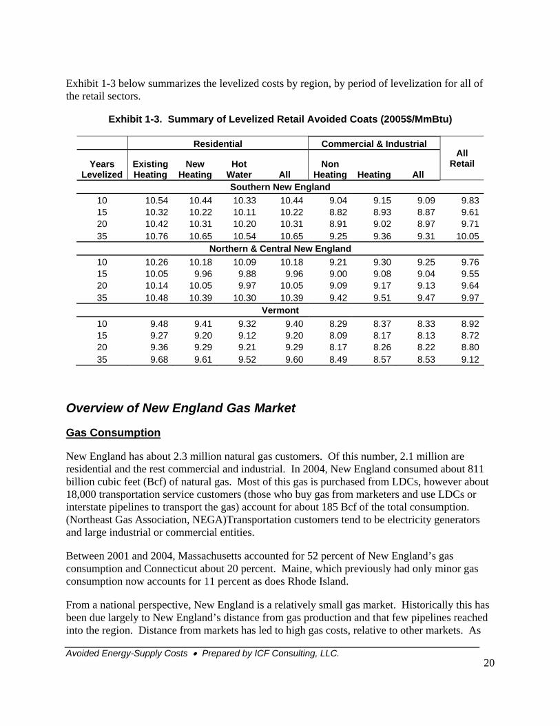
Exhibit 1-3 below summarizes the levelized costs by region, by period of levelization for all of the retail sectors.
Exhibit 1-3. Summary of Levelized Retail Avoided Coats (2005$/MmBtu)
Residential Commercial & Industrial
Years Levelized
Existing Heating
New Heating
Hot Water All
Non Heating Heating All
All Retail
Southern New England 10 10.54 10.44 10.33 10.44 9.04 9.15 9.09 9.8315 10.32 10.22 10.11 10.22 8.82 8.93 8.87 9.6120 10.42 10.31 10.20 10.31 8.91 9.02 8.97 9.7135 10.76 10.65 10.54 10.65 9.25 9.36 9.31 10.05
Northern & Central New England 10 10.26 10.18 10.09 10.18 9.21 9.30 9.25 9.7615 10.05 9.96 9.88 9.96 9.00 9.08 9.04 9.5520 10.14 10.05 9.97 10.05 9.09 9.17 9.13 9.6435 10.48 10.39 10.30 10.39 9.42 9.51 9.47 9.97
Vermont 10 9.48 9.41 9.32 9.40 8.29 8.37 8.33 8.9215 9.27 9.20 9.12 9.20 8.09 8.17 8.13 8.7220 9.36 9.29 9.21 9.29 8.17 8.26 8.22 8.8035 9.68 9.61 9.52 9.60 8.49 8.57 8.53 9.12
Overview of New England Gas Market
Gas Consumption
New England has about 2.3 million natural gas customers. Of this number, 2.1 million are residential and the rest commercial and industrial. In 2004, New England consumed about 811 billion cubic feet (Bcf) of natural gas. Most of this gas is purchased from LDCs, however about 18,000 transportation service customers (those who buy gas from marketers and use LDCs or interstate pipelines to transport the gas) account for about 185 Bcf of the total consumption. (Northeast Gas Association, NEGA)Transportation customers tend to be electricity generators and large industrial or commercial entities.
Between 2001 and 2004, Massachusetts accounted for 52 percent of New England’s gas consumption and Connecticut about 20 percent. Maine, which previously had only minor gas consumption now accounts for 11 percent as does Rhode Island.
From a national perspective, New England is a relatively small gas market. Historically this has been due largely to New England’s distance from gas production and that few pipelines reached into the region. Distance from markets has led to high gas costs, relative to other markets. As
Avoided Energy-Supply Costs • Prepared by ICF Consulting, LLC.
21
such, gas’ share of the heating market in New England is smaller than that of New York and many other states: gas accounts for 33 percent of the home heating market, oil for 49 percent. (NEGA)
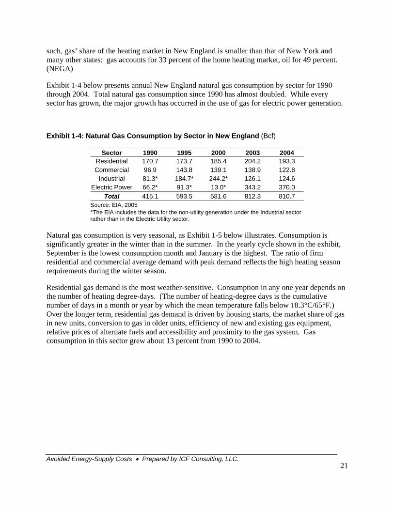
Exhibit 1-4 below presents annual New England natural gas consumption by sector for 1990 through 2004. Total natural gas consumption since 1990 has almost doubled. While every sector has grown, the major growth has occurred in the use of gas for electric power generation.
Exhibit 1-4: Natural Gas Consumption by Sector in New England (Bcf)
Sector 1990 1995 2000 2003 2004 Residential 170.7 173.7 185.4 204.2 193.3 Commercial 96.9 143.8 139.1 138.9 122.8
Industrial 81.3* 184.7* 244.2* 126.1 124.6 Electric Power 66.2* 91.3* 13.0* 343.2 370.0
Total 415.1 593.5 581.6 812.3 810.7 Source: EIA, 2005 *The EIA includes the data for the non-utility generation under the Industrial sector rather than in the Electric Utility sector.
Natural gas consumption is very seasonal, as Exhibit 1-5 below illustrates. Consumption is significantly greater in the winter than in the summer. In the yearly cycle shown in the exhibit, September is the lowest consumption month and January is the highest. The ratio of firm residential and commercial average demand with peak demand reflects the high heating season requirements during the winter season.
Residential gas demand is the most weather-sensitive. Consumption in any one year depends on the number of heating degree-days. (The number of heating-degree days is the cumulative number of days in a month or year by which the mean temperature falls below 18.3°C/65°F.) Over the longer term, residential gas demand is driven by housing starts, the market share of gas in new units, conversion to gas in older units, efficiency of new and existing gas equipment, relative prices of alternate fuels and accessibility and proximity to the gas system. Gas consumption in this sector grew about 13 percent from 1990 to 2004.
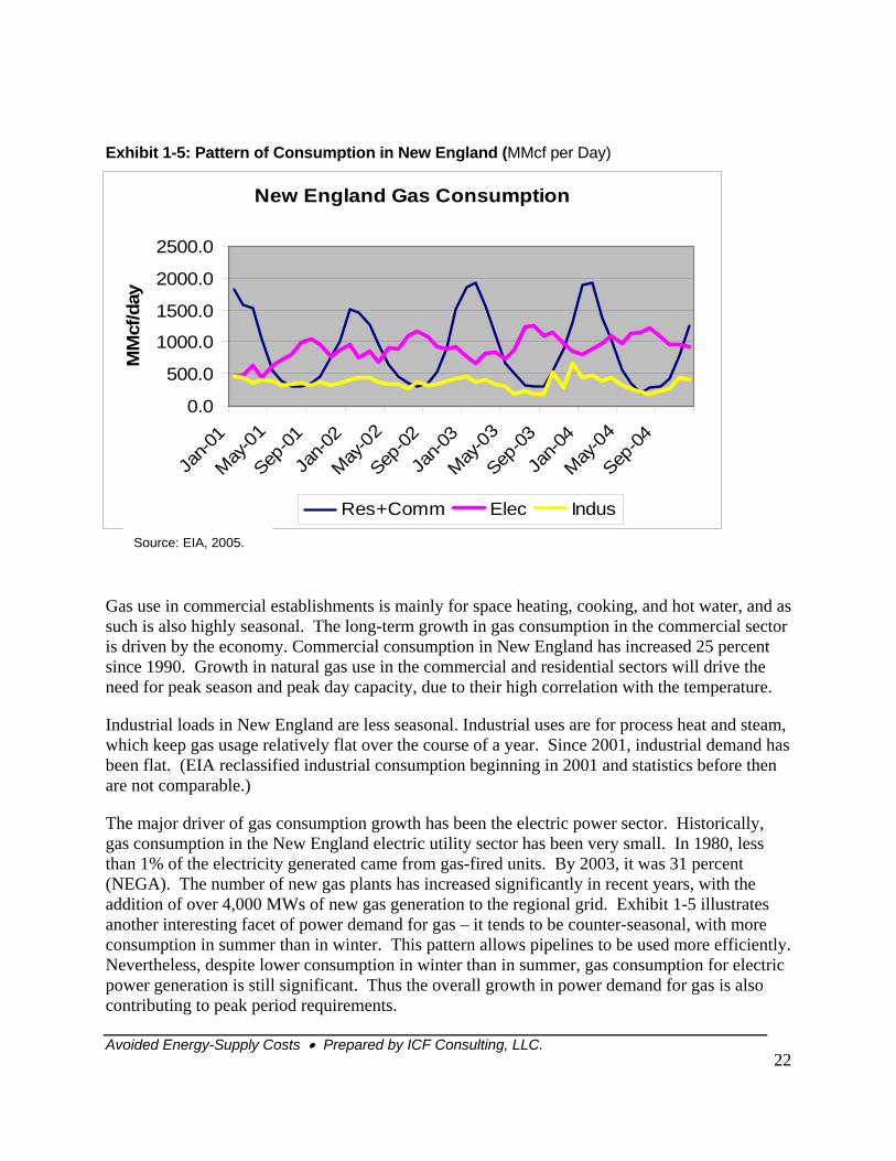
Exhibit 1-5: Pattern of Consumption in New England (MMcf per Day)
New England Gas Consumption
0.0
500.0
1000.0
1500.0
2000.0
2500.0
Jan-0
1
May-0
1
Sep-01
Jan-0
2
May-0
2
Sep-02
Jan-0
3
May-0
3
Sep-03
Jan-0
4
May-0
4
Sep-04
MM
cf/d
ay
Res+Comm Elec Indus
Source: EIA, 2005.
Gas use in commercial establishments is mainly for space heating, cooking, and hot water, and as such is also highly seasonal. The long-term growth in gas consumption in the commercial sector is driven by the economy. Commercial consumption in New England has increased 25 percent since 1990. Growth in natural gas use in the commercial and residential sectors will drive the need for peak season and peak day capacity, due to their high correlation with the temperature.
Industrial loads in New England are less seasonal. Industrial uses are for process heat and steam, which keep gas usage relatively flat over the course of a year. Since 2001, industrial demand has been flat. (EIA reclassified industrial consumption beginning in 2001 and statistics before then are not comparable.)
The major driver of gas consumption growth has been the electric power sector. Historically, gas consumption in the New England electric utility sector has been very small. In 1980, less than 1% of the electricity generated came from gas-fired units. By 2003, it was 31 percent (NEGA). The number of new gas plants has increased significantly in recent years, with the addition of over 4,000 MWs of new gas generation to the regional grid. Exhibit 1-5 illustrates another interesting facet of power demand for gas – it tends to be counter-seasonal, with more consumption in summer than in winter. This pattern allows pipelines to be used more efficiently. Nevertheless, despite lower consumption in winter than in summer, gas consumption for electric power generation is still significant. Thus the overall growth in power demand for gas is also contributing to peak period requirements.
Avoided Energy-Supply Costs • Prepared by ICF Consulting, LLC.
22
Avoided Energy-Supply Costs • Prepared by ICF Consulting, LLC.
23
The EIA Annual Energy Outlook for 2005 projects New England gas consumption will grow about 1.4 percent annually through 2025. Much of this growth will be in the power sector.
Gas Supply
Five interstate pipelines and one LNG import facility serve the New England market by bringing in gas supply from the U.S. Gulf Coast and both western and eastern Canada. LNG comes from a variety of areas, principally from Trinidad and Tobago. (See Exhibit 1-6.)
• The major pipeline serving New England is Tennessee Gas Pipeline (TGP). TGP supplies gas from the U.S. Gulf Coast, and has interconnections with upstream pipelines with access to western Canada and the U.S. Midwest. TGP is owned by El Paso Corp. TGP has major interconnections for Canadian supplies at Niagara, New York, with TransCanada Pipelines (TCPL) and at Wright, New York with Iroquois Gas Transmission System (Iroquois).
• The Algonquin Gas Transmission System (AGT) and its upstream sister pipeline, Texas Eastern Transmission Company (TETCO), both owned by Duke Energy, serve much of southern New England and reaches to the Boston area. AGT via TETCO also has direct access to the Gulf Coast; with its interconnection with Iroquois it also has access to western Canadian gas. AGT in the last year has also become connected to the Maritimes and Northeast Pipeline (a Duke affiliate), via the Hub Line around Boston.
• Iroquois provides gas to both TGP and AGT and also serves LDCs directly in Connecticut. Iroquois is connected to TCPL at Waddington, New York, and terminates in Long Island. The Eastchester extension of Iroquois also reaches into New York City.
• The Portland Natural Gas Transmission System (PNGTS) enters New England from the northwest, providing direct access to western Canada via the upstream TransQuebec and Maritime Pipeline (TQM) and TCPL. The PNGTS provides gas to southern Maine, New Hampshire, and Massachusetts. For the last 101 miles, it shares pipeline space with Maritimes and Northeast.
• Maritimes and Northeast Pipeline enter New England from New Brunswick, Canada, and provide access to Sable Island gas supplies. Maritimes serves Maine but provides the bulk of its supply into the Boston market area at Dracut, Massachusetts, and via the Hub Line.
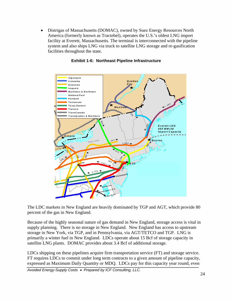
• Distrigas of Massachusetts (DOMAC), owned by Suez Energy Resources North America (formerly known as Tractebel), operates the U.S.’s oldest LNG import facility at Everett, Massachusetts. The terminal is interconnected with the pipeline system and also ships LNG via truck to satellite LNG storage and re-gasification facilities throughout the state.
Exhibit 1-6: Northeast Pipeline Infrastructure
B os ton
N YC
M o n tr ea l
Q ue b e cC ity
O nt a rio
13 7621
0
44 0236
850
C ove Po int
Ph iladelp hia
W ash ing to n, D .C.B altim ore
N EW YOR K
2,61 1
1,36
7
1,15
0
57 2
38 0L eidy
T o ta l C a p a c ityin to N ew Y o r k C ity is2 ,4 9 5 M M c fd
1,50 044 7
951
1,298
611
100
1,57
5
900200
2 ,73 5
A lg o n q u in
Iro q u o is
C o lu m b ia
D o m in io n
M a rit im e s & N o rth eas t
N at io n al F u elP o rt la n d
T e n n es seeT e xas E as te rnT ra n sc o
T ra n sC an a d aT ra n sQ u eb e c & M ar it im e s
E v er et t LN G4 5 0 M M c fdIm p or t C a p ac ity
The LDC markets in New England are heavily dominated by TGP and AGT, which provide 80 percent of the gas in New England.
Because of the highly seasonal nature of gas demand in New England, storage access is vital in supply planning. There is no storage in New England. New England has access to upstream storage in New York, via TGP, and in Pennsylvania, via AGT/TETCO and TGP. LNG is primarily a winter fuel in New England. LDCs operate about 15 Bcf of storage capacity in satellite LNG plants. DOMAC provides about 3.4 Bcf of additional storage.
LDCs shipping on these pipelines acquire firm transportation service (FT) and storage service. FT requires LDCs to commit under long term contracts to a given amount of pipeline capacity, expressed as Maximum Daily Quantity or MDQ. LDCs pay for this capacity year round, even Avoided Energy-Supply Costs • Prepared by ICF Consulting, LLC.
24
when it is only fully utilized during the heating season. LDCs can release or resell capacity into a secondary market for prices up to the rates charged by the pipeline. When considering the avoided costs of meeting peak demand, the full annual cost of pipeline capacity is taken into account, as explained more fully below.
For purposes of estimating avoided costs, the marginal source of gas can be considered the U.S. Gulf Coast, as represented by Henry Hub prices. Supplies from other areas like Sable Island and LNG are priced in reference to Gulf Coast supply. For deliveries into New England, we have used the TGP and TETCO-AGT systems along with their storage services. For peaking supplies, we have used the Distrigas LNG facility.
Gas Prices
Natural gas prices have increased significantly in the last several years, as has the overall volatility of gas prices... In this section we address both issues and consider the implications of these developments for avoided gas costs.
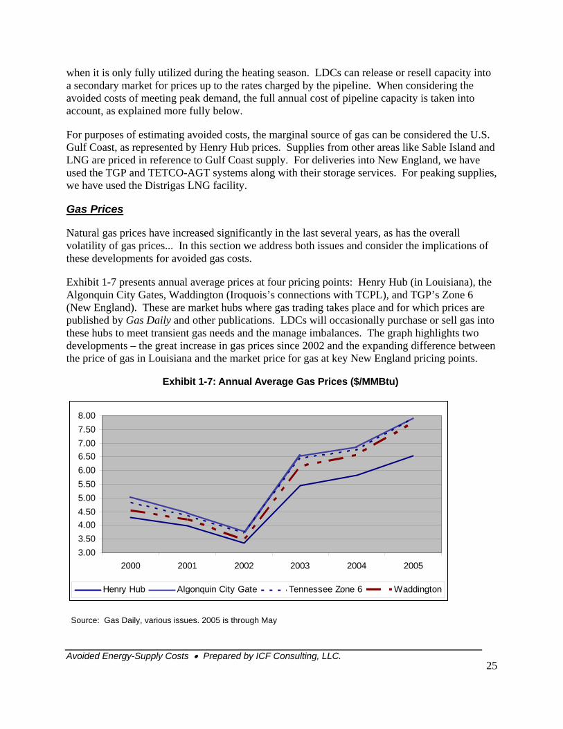
Exhibit 1-7 presents annual average prices at four pricing points: Henry Hub (in Louisiana), the Algonquin City Gates, Waddington (Iroquois’s connections with TCPL), and TGP’s Zone 6 (New England). These are market hubs where gas trading takes place and for which prices are published by Gas Daily and other publications. LDCs will occasionally purchase or sell gas into these hubs to meet transient gas needs and the manage imbalances. The graph highlights two developments – the great increase in gas prices since 2002 and the expanding difference between the price of gas in Louisiana and the market price for gas at key New England pricing points.
Exhibit 1-7: Annual Average Gas Prices ($/MMBtu)
3.003.504.004.505.005.506.006.507.007.508.00
2000 2001 2002 2003 2004 2005
Henry Hub Algonquin City Gate Tennessee Zone 6 Waddington
Source: Gas Daily, various issues. 2005 is through May
Avoided Energy-Supply Costs • Prepared by ICF Consulting, LLC.
25
The overall gas price increase is due to the general tightening of gas supplies in North America and the strong demand for gas. This is reflected in all markets, and as shown here, gas prices in New England follow Henry Hub prices.
The second notable aspect of the data is the expanding spread between New England prices and Henry Hub – this is referred to as the basis spread. Since 2002, the basis between Henry Hub and various New England pricing points has increased from about $0.50/MMBtu to over $1.00/MMBtu. In part this is a result of the overall increase in the price of gas and the resulting fuel cost for delivering it to New England. A major cause of the higher basis is the demand on gas capacity, which has bid up the price of delivered gas in New England. Thus the expanding price difference suggests a need for additional pipeline capacity and supply.
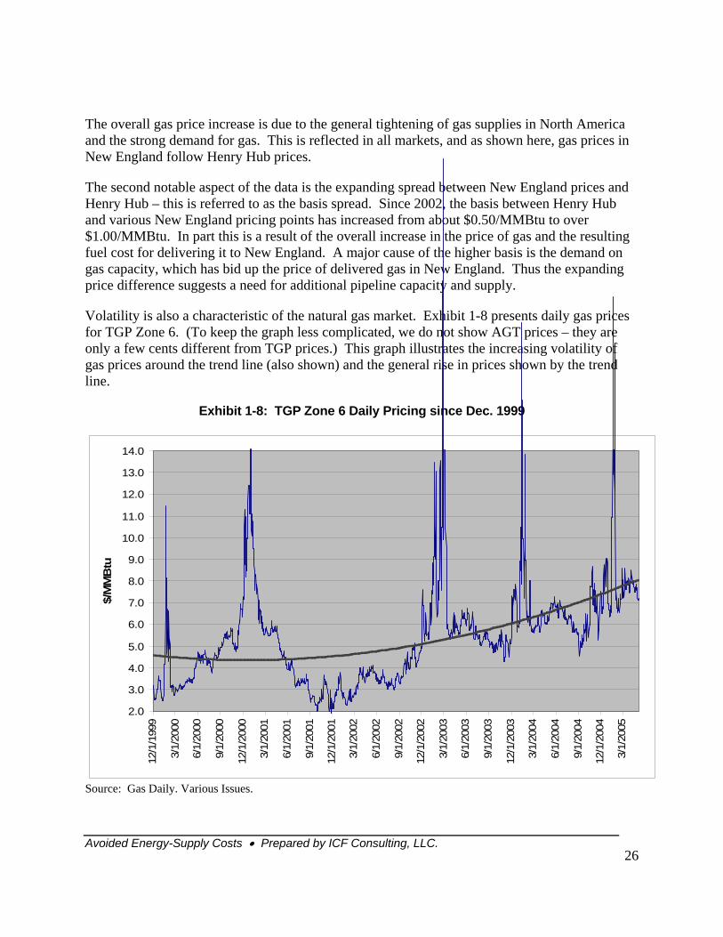
Volatility is also a characteristic of the natural gas market. Exhibit 1-8 presents daily gas prices for TGP Zone 6. (To keep the graph less complicated, we do not show AGT prices – they are only a few cents different from TGP prices.) This graph illustrates the increasing volatility of gas prices around the trend line (also shown) and the general rise in prices shown by the trend line.
Exhibit 1-8: TGP Zone 6 Daily Pricing since Dec. 1999
14.0
Avoided Energy-Supply Costs • Prepared by ICF Consulting, LLC.
26
2.0
3.0
4.0
12/1
/199
9
3/1/
2000
6/1/
2000
9/1/
2000
12/1
/200
0
3/1/
2001
6/1/
2001
9/1/
2001
12/1
/200
1
3/1/
2002
6/1/
2002
9/1/
2002
12/1
/200
2
3/1/
2003
6/1/
2003
9/1/
2003
12/1
/200
3
3/1/
2004
6/1/
2004
9/1/
2004
12/1
/200
4
3/20
05
5.0
12.0
13.0
1/
7.0
8.0
9.0
10.0
11.0
$/M
MB
tu
6.0
Source: Gas Daily. Various Issues.
Avoided Energy-Supply Costs • Prepared by ICF Consulting, LLC.
27
The spikes in gas prices correspond to winter periods when cold fronts sweep through New ds to reflect volatility at Henry Hub and not local volatility. This is
because LDCs (and most marketers) purchase gas in the producing areas and use firm
s
s r
and LNG service are calculated from the tariffs of the TGP and TETCO-AGT pipelines, their respective storage services, and the Distrigas LNG tariff. For each winter
ribed
, e
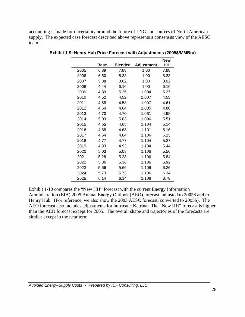
Exhibit 1-9 shows the development of the Henry Hub forecast used for this study. NANGAS® was used to develop f the blending of the “Base” forecast for the years 2005 through 2009 with current futures market forward prices. The blended price ra ct rices year-to-date (for 2005), futures prices, EIA ort te recas the Ba se fo . Beginning in 2005, the reported price is a blend of actual prices, fu and th shor forecast; in 2006, the price is a blend of EIA’s short term forecast an res; in the s a blend of mostly futures and the base fore or 20 d 200 base s blen ith futures prices, with the base assuming a shar h year. The Henry Hub prices for 2010 and beyond are based on a pure model-g ed ou . Thi stment was made to reflect current market conditions that are not captured in a long term sting such NGAS®. As noted earlier, the blending of th res a lects cent of K on near term gas prices through 2009.
The “Adjustment” column is a multiplier that termi the f a NANGAS® forecast using a pessimistic supply o k cas h yie ighe rices and the less pessimistic base case forecast. Bey 14, justm reas forecast prices by about 10 percent. The re fore how e “Ne ” col the product of the “Blended” and “Adjustm nd sh e co ed an ted c here some
England. LDC pricing ten
transportation to ship gas to New England. This gas is bought and priced at first of the month indices. Daily pricing reflects transient conditions in the market – weather, for example. LDCmay occasionally buy gas in this short term market to meet balancing obligations.
Methodology
Our approach to estimating the avoided cost is to identify the costs avoided by a LDC from not having to buy a marginal Mcf of gas. The components of the avoided costs are the cost of gas,transportation, winter storage, and winter peaking LNG. The forecast cost of gas as described below is estimated from ICF’s North American Natural Gas Analysis System (NANGAS®). Thigenerated a Henry Hub price. We used historic seasonal volatility to estimate the summer/wintedifferentials for each of the winter types stipulated for the avoided cost study. The costs of transportation, storage,
type, we estimated the share of service provided by pipeline gas, storage, and LNG, as descbelow in the section titled “Delivery Costs to New England.” Annual capacity charges were allocated to the appropriate winter types by dividing by the number of days in each type. Thusthe avoided cost for any winter type represents the avoidance of the marginal Mcf of gas and thallocation of the avoided capacity costs to that winter type.
Henry Hub Prices
the “Base” outlook for gas prices. The “Blended” column shows the results o
incorpo tes several elements: a ual p’s sh rm fo t, and se ca recast
tures e EIA t termd futu 2007 price i
cast; f 08 an 9, the case i ded w larger e eacenerat tlook s adju
foreca model as NAe futu lso ref the re impact atrina
was de ned by ratio outloo e whic lded h r gas p
ond 20 this ad ent inc ed thesulting cast s n in th w HH umn isent” a ould b nsider expec ase, w
Avoided Energy-Supply Costs • Prepared by ICF Consulting, LLC.
28
accounting is made for u inty a the of LN sou f North American supply. The expected ca cast bed repre conteam.
Exhibit 1-9: H ub ore ith A ent 5$/MMBtu)
ncerta round future G and rces ose fore descri above sents a sensus view of the AESC
enry H Price F cast w djustm s (200
Base Blended Adjustment HH New
2005 6.89 7.88 1.00 7.88 2006 6.50 8.33 1.00 8.33 2007 5.38 8.02 1.00 8.02 2008 4.44 6.16 1.00 6.16 2009 4.39 5.25 1.004 5.27 2010 4.52 4.52 1.007 4.55 2011 4.58 4.58 1.007 4.61 2012 4.64 4.64 1.035 4.80 2013 4.70 4.70 1.061 4.98 2014 5.03 5.03 1.096 5.51 2015 4.65 4.65 1.104 5.14 2016 4.68 4.68 1.101 5.16 2017 4.64 4.64 1.106 5.13 2018 4.77 4.77 1.104 5.27 2019 4.93 4.93 1.104 5.44 2020 5.03 5.03 1.106 5.56 2021 5.28 5.28 1.106 5.84 2022 5.36 5.36 1.106 5.92 2023 5.66 5.66 1.106 6.26 2024 5.73 5.73 1.106 6.34 2025 6.14 6.14 1.106 6.79
Exhibit 1-10 compares the “New HH” forecast with the current Energy Information Administration (EIA) 2005 Annual Energy Outlook (AEO) forecast, adjusted to 2005$ and to Henry Hub. (For reference, we also show the 2003 AESC forecast, converted to 2005$). The AEO forecast also includes adjustments for hurricane Katrina. The “New HH” forecast is higher than the AEO forecast except for 2005. The overall shape and trajectories of the forecasts are similar except in the near term.
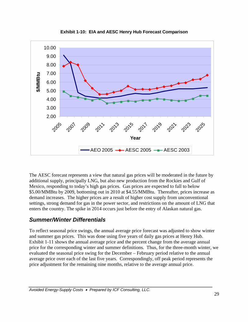
Exhibit 1-10: EIA and AESC Henry Hub Forecast Comparison
2.00
3.00
4.00
5.00
6.00
7.00
8.00
9.00
10.00
2005
2007
2009
2011
2013
2015
2017
2019
2021
2023
2025
Year
$/M
MB
tu
AEO 2005 AESC 2005 AESC 2003
The AESC forecast represents a view that natural gas prices will be moderated in the future by additional supply, principally LNG, but also new production from the Rockies and Gulf of Mexico, responding to today’s high gas prices. Gas prices are expected to fall to below $5.00/MMBtu by 2009, bottoming out in 2010 at $4.55/MMBtu. Thereafter, prices increase as demand increases. The higher prices are a result of higher cost supply from unconventional settings, strong demand for gas in the power sector, and restrictions on the amount of LNG that enters the country. The spike in 2014 occurs just before the entry of Alaskan natural gas.
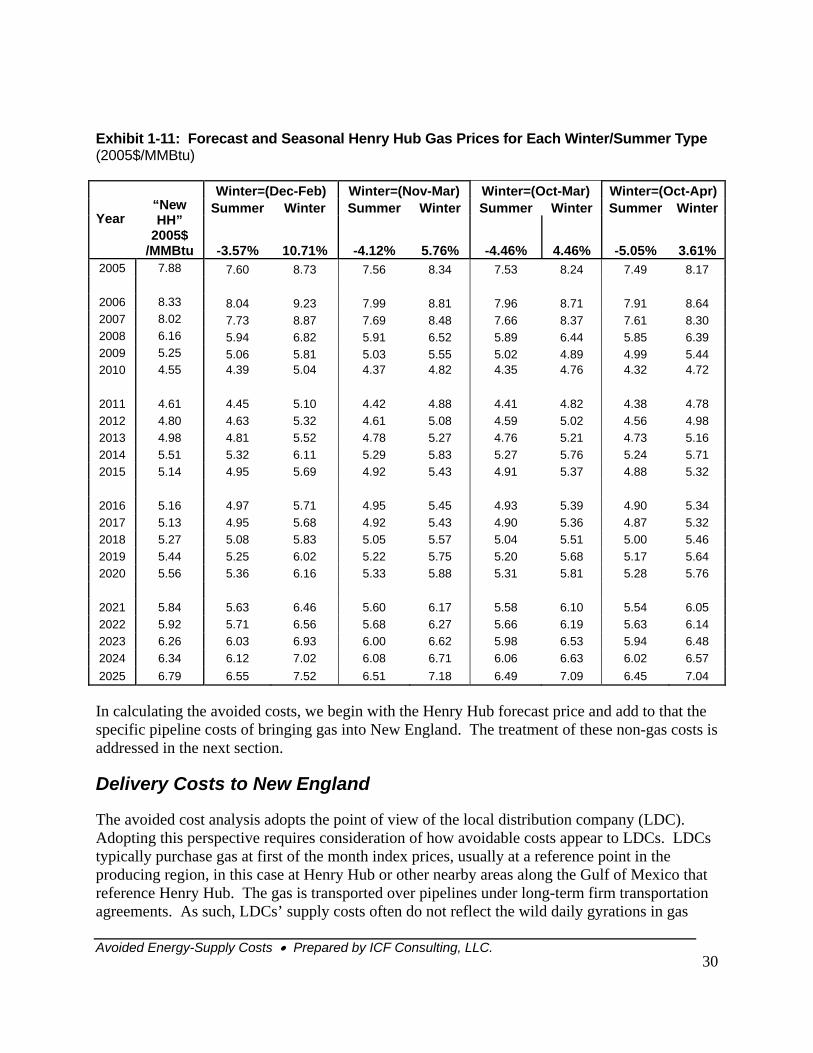
Summer/Winter Differentials
To reflect seasonal price swings, the annual average price forecast was adjusted to show winter and summer gas prices. This was done using five years of daily gas prices at Henry Hub. Exhibit 1-11 shows the annual average price and the percent change from the average annual price for the corresponding winter and summer definitions. Thus, for the three-month winter, we evaluated the seasonal price swing for the December – February period relative to the annual average price over each of the last five years. Correspondingly, off peak period represents the price adjustment for the remaining nine months, relative to the average annual price.
Avoided Energy-Supply Costs • Prepared by ICF Consulting, LLC.
29
Avoided Energy-Supply Costs • Prepared by ICF Consulting, LLC.
30
Exhibit 1-11: Forecast and Seasonal Henry Hub Gas Prices for Each Winter/Summer Type (2005$/MMBtu)
Winter=(Dec-Feb) Winter=(Nov-Mar) Winter=(Oct-Mar) Winter=(Oct-Apr) Summer Winter Summer Winter Summer Winter Summer Winter
Year
“New HH”
2005$ /MMBtu -3.57% 10.71% -4.12% 5.76% -4.46% 4.46% -5.05% 3.61%
2005 7.88 7.60 8.73 7.56 8.34 7.53 8.24 7.49 8.17
2006 8.33 8.04 9.23 7.99 8.81 7.96 8.71 7.91 8.64 2007 8.02 7.73 8.87 7.69 8.48 7.66 8.37 7.61 8.30 2008 6.16 5.94 6.82 5.91 6.52 5.89 6.44 5.85 6.39 2009 5.25 5.06 5.81 5.03 5.55 5.02 4.89 4.99 5.44 2010 4.55 4.39 5.04 4.37 4.82 4.35 4.76 4.32 4.72
2011 4.61 4.45 5.10 4.42 4.88 4.41 4.82 4.38 4.78 2012 4.80 4.63 5.32 4.61 5.08 4.59 5.02 4.56 4.98 2013 4.98 4.81 5.52 4.78 5.27 4.76 5.21 4.73 5.16 2014 5.51 5.32 6.11 5.29 5.83 5.27 5.76 5.24 5.71 2015 5.14 4.95 5.69 4.92 5.43 4.91 5.37 4.88 5.32
2016 5.16 4.97 5.71 4.95 5.45 4.93 5.39 4.90 5.34 2017 5.13 4.95 5.68 4.92 5.43 4.90 5.36 4.87 5.32 2018 5.27 5.08 5.83 5.05 5.57 5.04 5.51 5.00 5.46 2019 5.44 5.25 6.02 5.22 5.75 5.20 5.68 5.17 5.64 2020 5.56 5.36 6.16 5.33 5.88 5.31 5.81 5.28 5.76
2021 5.84 5.63 6.46 5.60 6.17 5.58 6.10 5.54 6.05 2022 5.92 5.71 6.56 5.68 6.27 5.66 6.19 5.63 6.14 2023 6.26 6.03 6.93 6.00 6.62 5.98 6.53 5.94 6.48 2024 6.34 6.12 7.02 6.08 6.71 6.06 6.63 6.02 6.57 2025 6.79 6.55 7.52 6.51 7.18 6.49 7.09 6.45 7.04
In calculating the avoided costs, we begin with the Henry Hub forecast price and add to that the specific pipeline costs of bringing gas into New England. The treatment of these non-gas costs is addressed in the next section.
Delivery Costs to New England
The avoided cost analysis adopts the point of view of the local distribution company (LDC). Adopting this perspective requires consideration of how avoidable costs appear to LDCs. LDCs typically purchase gas at first of the month index prices, usually at a reference point in the producing region, in this case at Henry Hub or other nearby areas along the Gulf of Mexico that reference Henry Hub. The gas is transported over pipelines under long-term firm transportation agreements. As such, LDCs’ supply costs often do not reflect the wild daily gyrations in gas
Avoided Energy-Supply Costs • Prepared by ICF Consulting, LLC.
31
prices that characterize the northeastern markets. (LDCs do enter daily markets to supplement supplies and manage imbalances.)
To meet winter demands, LDCs supplement pipeline-transported supplies with storage and peak shaving, the latter in New England being largely liquefied natural gas (LNG). LDCs purchase capacity on an annual basis and pay the reservation charges (or demand charges) for each MMBtu of reserved capacity (or maximum daily quantity – MDQ) for an entire year, payable in twelve monthly payments.
Thus, when a LDC avoids having to meet demand in the winter, the LDC can in turn avoid the capacity reservation charges associated with meeting an incremental unit of demand for the peak period. Despite being under long-term contracts for service, reservation charges are avoidable because of the capacity release market. LDCs can release un-needed capacity usually at full rates for winter service. However, when an LDC avoids having to meet demand in the summer, it avoids only having to purchase and transport an incremental MMBtu of gas. Because capacity is in excess supply in the summer, the pipeline capacity value is nearly zero, and thus is not avoidable.
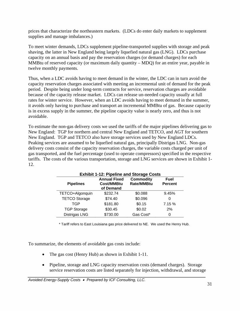
To estimate the non-gas delivery costs we used the tariffs of the major pipelines delivering gas to New England: TGP for northern and central New England and TETCO, and AGT for southern New England. TGP and TETCO also have storage services used by New England LDCs. Peaking services are assumed to be liquefied natural gas, principally Distrigas LNG. Non-gas delivery costs consist of the capacity reservation charges, the variable costs charged per unit of gas transported, and the fuel percentage (used to operate compressors) specified in the respective tariffs. The costs of the various transportation, storage and LNG services are shown in Exhibit 1-12.
Exhibit 1-12: Pipeline and Storage Costs
Pipelines Annual Fixed Cost/MMBtu of Demand
Commodity Rate/MMBtu
Fuel Percent
TETCO+Algonquin $232.74 $0.088 9.45% TETCO Storage $74.40 $0.096 0
TGP $181.80 $0.15 7.15 % TGP Storage $30.45 $0.02 2% Distrigas LNG $730.00 Gas Cost* 0
* Tariff refers to East Louisiana gas price delivered to NE. We used the Henry Hub.
To summarize, the elements of avoidable gas costs include:
• The gas cost (Henry Hub) as shown in Exhibit 1-11.
• Pipeline, storage and LNG capacity reservation costs (demand charges). Storage service reservation costs are listed separately for injection, withdrawal, and storage
Avoided Energy-Supply Costs • Prepared by ICF Consulting, LLC.
32
capacity. LNG reservation costs include a re-gasification capacity charge and a storage space charge. These costs, shown in column one of Exhibit 1-12, are allocated on a per unit basis by dividing the annual costs by the number of days in the appropriate winter periods.
• The variable costs associated with transportation, storage and LNG. This consists of the commodity or usage rate and the fuel charge from the pipeline transportation, storage, and LNG tariffs as shown in the second column in Exhibit 1-12, above. The fuel charge is calculated as a percent of the cost of the natural gas and is included in the commodity rate.
Our general approach recognizes that reservation charges are incurred to meet peak winter demand. Thus, the winter avoided costs equal the sum of the Henry Hub price, the variable transportation costs on the appropriate pipeline, and the cost of a year’s worth of capacity payments for transportation, storage and LNG allocated to the winter days for each winter type. The avoided cost in the summer is simply the Henry Hub price and the variable costs of transportation.
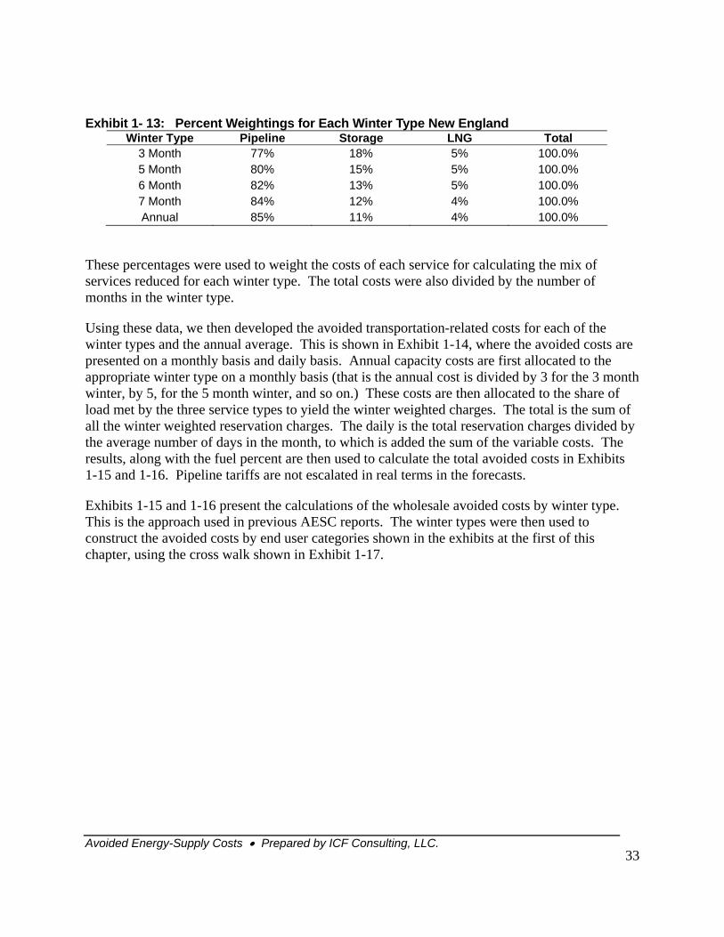
One step in the analysis was determining the share of winter reservation costs that are attributable to pipeline, storage and peak shaving reservation charges. The mix of pipeline transported gas, storage, and LNG for a typical LDC is optimized around that LDC’s particular load shape. That is, LDCs purchase a mix of capacity that allows them to meet peak loads at lowest cost. For example, the amount of storage capacity will be determined by its cost, relative to the cost of pipeline and peak shaving capacity for the LDC’s particular load characteristics. Changes in the shape of the load due to conservation and load management (C&LM) programs thus have cost impacts across all supply options, and not just on the marginal supply source, such as LNG or storage. This is because LNG service or storage service is sized in conjunction with pipeline capacity. A reduction in the need for a marginal unit of LNG or storage gas affects the amount of pipeline capacity needed. For this analysis we approximated this optimization across LDCs in New England, by reducing all service options – pipeline, storage, LNG – roughly in the proportion to how these services are normally deployed by the LDCs to meet winter loads. For this we used data provided by NSTAR and KeySpan that showed for each month of the year which services were deployed to meet the system sales sendout. In general, we saw the following relationships for each of the winter types (Exhibit 1-13):
Avoided Energy-Supply Costs • Prepared by ICF Consulting, LLC.
33
Exhibit 1- 13: Percent Weightings for Each Winter Type New England Winter Type Pipeline Storage LNG Total
3 Month 77% 18% 5% 100.0% 5 Month 80% 15% 5% 100.0% 6 Month 82% 13% 5% 100.0% 7 Month 84% 12% 4% 100.0% Annual 85% 11% 4% 100.0%
These percentages were used to weight the costs of each service for calculating the mix of services reduced for each winter type. The total costs were also divided by the number of months in the winter type.
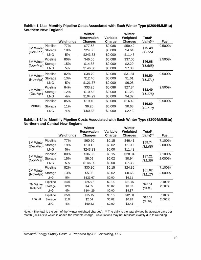
Using these data, we then developed the avoided transportation-related costs for each of the winter types and the annual average. This is shown in Exhibit 1-14, where the avoided costs are presented on a monthly basis and daily basis. Annual capacity costs are first allocated to the appropriate winter type on a monthly basis (that is the annual cost is divided by 3 for the 3 month winter, by 5, for the 5 month winter, and so on.) These costs are then allocated to the share of load met by the three service types to yield the winter weighted charges. The total is the sum of all the winter weighted reservation charges. The daily is the total reservation charges divided by the average number of days in the month, to which is added the sum of the variable costs. The results, along with the fuel percent are then used to calculate the total avoided costs in Exhibits 1-15 and 1-16. Pipeline tariffs are not escalated in real terms in the forecasts.
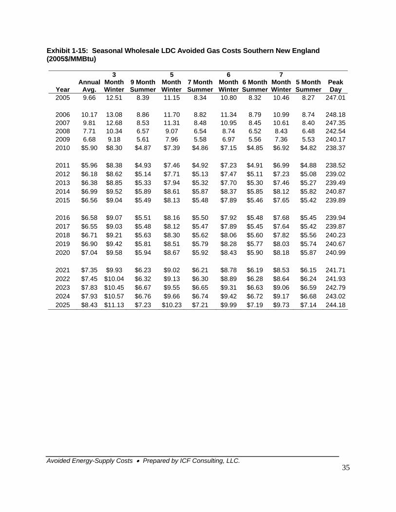
Exhibits 1-15 and 1-16 present the calculations of the wholesale avoided costs by winter type. This is the approach used in previous AESC reports. The winter types were then used to construct the avoided costs by end user categories shown in the exhibits at the first of this chapter, using the cross walk shown in Exhibit 1-17.
Avoided Energy-Supply Costs • Prepared by ICF Consulting, LLC.
34
Exhibit 1-14a: Monthly Pipeline Costs Associated with Each Winter Type ($2004/MMBtu) Southern New England
Weightings
Winter Reservation
Charges Variable Charge
Winter Weighted Charges
Total* (daily)** Fuel
Pipeline 77% $77.58 $0.088 $59.42 9.500% Storage 18% $24.80 $0.000 $4.64 3M Winter
(Dec-Feb) LNG 5% $243.33 $0.000 $11.43
$75.49 ($2.55)
Pipeline 80% $46.55 $0.088 $37.05 9.500% Storage 15% $14.88 $0.000 $2.29 5M Winter
(Nov-Mar) LNG 5% $146.00 $0.000 $7.33
$46.68 ($1.605)
Pipeline 82% $38.79 $0.088 $31.81 9.500% Storage 13% $12.40 $0.000 $1.61
6M Winter (Nov-Apr)
LNG 5% $121.67 $0.000 $6.08
$39.50 ($1.371)
Pipeline 84% $33.25 $0.088 $27.84 9.500% Storage 12% $10.63 $0.000 $1.28 7M Winter
(Oct-Apr) LNG 4% $104.29 $0.000 $4.37
$33.49 ($1.175)
Pipeline 85% $19.40 $0.088 $16.49 9.500% Storage 11% $6.20 $0.000 $0.68 Annual
LNG 4% $60.83 $0.000 $2.43
$19.60 ($0.719)
Exhibit 1-14b: Monthly Pipeline Costs Associated with Each Winter Type ($2004/MMBtu) Northern and Central New England
Weightings
Winter Reservation
Charges Variable Charge
Winter Weighted Charges
Total* (daily)** Fuel
Pipeline 77% $60.60 $0.15 $46.41 7.100% Storage 19% $10.15 $0.02 $1.90 2.000%
3M Winter (Dec-Feb)
LNG 5% $243.33 $0.00 $11.43
$59.74 ($2.08)
Pipeline 80% $36.36 $0.15 $28.94 7.100% Storage 15% $6.09 $0.02 $0.94 2.000% 5M Winter
(Nov-Mar) LNG 5% $146.00 $0.00 $7.33
$37.21 ($1.35)
Pipeline 82% $30.30 $0.15 $24.85 7.100% Storage 13% $5.08 $0.02 $0.66 2.000%
6M Winter (Nov-Apr)
LNG 5% $121.67 $0.00 $6.11
$31.62 ($1.17)
Pipeline 84% $25.97 $0.15 $21.75 7.100% Storage 12% $4.35 $0.02 $0.53 2.000% 7M Winter
(Oct-Apr) LNG 4% $104.29 $0.00 $4.37
$26.64 ($1.00)
Pipeline 85% $15.15 $0.15 $12.88 7.100% Storage 11% $2.54 $0.02 $0.28 2.000% Annual
LNG 4% $60.83 $0.00 $2.43
$15.59 ($0.64)
Note: * The total is the sum of the “winter weighted charges”. ** The daily is the total divided by average days per month (30.417) to which is added the variable charge. Calculations may not replicate exactly due to rounding.
Avoided Energy-Supply Costs • Prepared by ICF Consulting, LLC.
35
Exhibit 1-15: Seasonal Wholesale LDC Avoided Gas Costs Southern New England (2005$/MMBtu)
Year Annual
Avg.
3 Month Winter
9 Month Summer
5 Month Winter
7 Month Summer
6 Month Winter
6 Month Summer
7 Month Winter
5 Month Summer
Peak Day
2005 9.66 12.51 8.39 11.15 8.34 10.80 8.32 10.46 8.27 247.01
2006 10.17 13.08 8.86 11.70 8.82 11.34 8.79 10.99 8.74 248.182007 9.81 12.68 8.53 11.31 8.48 10.95 8.45 10.61 8.40 247.352008 7.71 10.34 6.57 9.07 6.54 8.74 6.52 8.43 6.48 242.542009 6.68 9.18 5.61 7.96 5.58 6.97 5.56 7.36 5.53 240.172010 $5.90 $8.30 $4.87 $7.39 $4.86 $7.15 $4.85 $6.92 $4.82 238.37
2011 $5.96 $8.38 $4.93 $7.46 $4.92 $7.23 $4.91 $6.99 $4.88 238.522012 $6.18 $8.62 $5.14 $7.71 $5.13 $7.47 $5.11 $7.23 $5.08 239.022013 $6.38 $8.85 $5.33 $7.94 $5.32 $7.70 $5.30 $7.46 $5.27 239.492014 $6.99 $9.52 $5.89 $8.61 $5.87 $8.37 $5.85 $8.12 $5.82 240.872015 $6.56 $9.04 $5.49 $8.13 $5.48 $7.89 $5.46 $7.65 $5.42 239.89
2016 $6.58 $9.07 $5.51 $8.16 $5.50 $7.92 $5.48 $7.68 $5.45 239.942017 $6.55 $9.03 $5.48 $8.12 $5.47 $7.89 $5.45 $7.64 $5.42 239.872018 $6.71 $9.21 $5.63 $8.30 $5.62 $8.06 $5.60 $7.82 $5.56 240.232019 $6.90 $9.42 $5.81 $8.51 $5.79 $8.28 $5.77 $8.03 $5.74 240.672020 $7.04 $9.58 $5.94 $8.67 $5.92 $8.43 $5.90 $8.18 $5.87 240.99
2021 $7.35 $9.93 $6.23 $9.02 $6.21 $8.78 $6.19 $8.53 $6.15 241.712022 $7.45 $10.04 $6.32 $9.13 $6.30 $8.89 $6.28 $8.64 $6.24 241.932023 $7.83 $10.45 $6.67 $9.55 $6.65 $9.31 $6.63 $9.06 $6.59 242.792024 $7.93 $10.57 $6.76 $9.66 $6.74 $9.42 $6.72 $9.17 $6.68 243.022025 $8.43 $11.13 $7.23 $10.23 $7.21 $9.99 $7.19 $9.73 $7.14 244.18
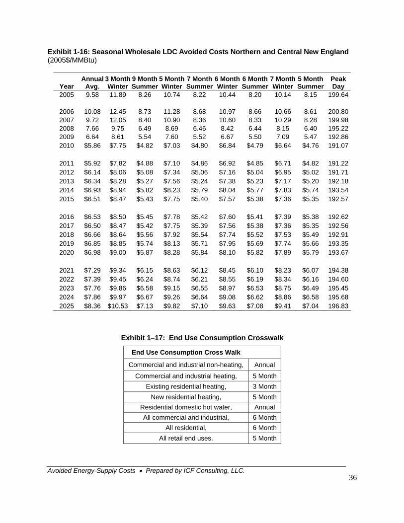
Avoided Energy-Supply Costs • Prepared by ICF Consulting, LLC.
36
Exhibit 1-16: Seasonal Wholesale LDC Avoided Costs Northern and Central New England (2005$/MMBtu)
Year Annual
Avg. 3 Month Winter
9 Month Summer
5 MonthWinter
7 Month Summer
6 Month Winter
6 Month Summer
7 Month Winter
5 Month Summer
Peak Day
2005 9.58 11.89 8.26 10.74 8.22 10.44 8.20 10.14 8.15 199.64
2006 10.08 12.45 8.73 11.28 8.68 10.97 8.66 10.66 8.61 200.802007 9.72 12.05 8.40 10.90 8.36 10.60 8.33 10.29 8.28 199.982008 7.66 9.75 6.49 8.69 6.46 8.42 6.44 8.15 6.40 195.222009 6.64 8.61 5.54 7.60 5.52 6.67 5.50 7.09 5.47 192.862010 $5.86 $7.75 $4.82 $7.03 $4.80 $6.84 $4.79 $6.64 $4.76 191.07
2011 $5.92 $7.82 $4.88 $7.10 $4.86 $6.92 $4.85 $6.71 $4.82 191.222012 $6.14 $8.06 $5.08 $7.34 $5.06 $7.16 $5.04 $6.95 $5.02 191.712013 $6.34 $8.28 $5.27 $7.56 $5.24 $7.38 $5.23 $7.17 $5.20 192.182014 $6.93 $8.94 $5.82 $8.23 $5.79 $8.04 $5.77 $7.83 $5.74 193.542015 $6.51 $8.47 $5.43 $7.75 $5.40 $7.57 $5.38 $7.36 $5.35 192.57
2016 $6.53 $8.50 $5.45 $7.78 $5.42 $7.60 $5.41 $7.39 $5.38 192.622017 $6.50 $8.47 $5.42 $7.75 $5.39 $7.56 $5.38 $7.36 $5.35 192.562018 $6.66 $8.64 $5.56 $7.92 $5.54 $7.74 $5.52 $7.53 $5.49 192.912019 $6.85 $8.85 $5.74 $8.13 $5.71 $7.95 $5.69 $7.74 $5.66 193.352020 $6.98 $9.00 $5.87 $8.28 $5.84 $8.10 $5.82 $7.89 $5.79 193.67
2021 $7.29 $9.34 $6.15 $8.63 $6.12 $8.45 $6.10 $8.23 $6.07 194.382022 $7.39 $9.45 $6.24 $8.74 $6.21 $8.55 $6.19 $8.34 $6.16 194.602023 $7.76 $9.86 $6.58 $9.15 $6.55 $8.97 $6.53 $8.75 $6.49 195.452024 $7.86 $9.97 $6.67 $9.26 $6.64 $9.08 $6.62 $8.86 $6.58 195.682025 $8.36 $10.53 $7.13 $9.82 $7.10 $9.63 $7.08 $9.41 $7.04 196.83
Exhibit 1–17: End Use Consumption Crosswalk
End Use Consumption Cross Walk
Commercial and industrial non-heating, Annual
Commercial and industrial heating, 5 Month Existing residential heating, 3 Month
New residential heating, 5 Month Residential domestic hot water, Annual All commercial and industrial, 6 Month
All residential, 6 Month All retail end uses. 5 Month
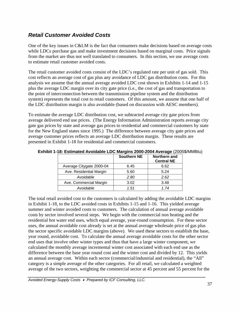
Avoided Energy-Supply Costs • Prepared by ICF Consulting, LLC.
37
Retail Customer Avoided Costs
One of the key issues in C&LM is the fact that consumers make decisions based on average costs while LDCs purchase gas and make investment decisions based on marginal costs. Price signals from the market are thus not well translated to consumers. In this section, we use average costs to estimate retail customer avoided costs.
The retail customer avoided costs consist of the LDC’s regulated rate per unit of gas sold. This cost reflects an average cost of gas plus any avoidance of LDC gas distribution costs. For this analysis we assume that the annual average avoided LDC cost shown in Exhibits 1-14 and 1-15 plus the average LDC margin over its city gate price (i.e., the cost of gas and transportation to the point of interconnection between the transmission pipeline system and the distribution system) represents the total cost to retail customers. Of this amount, we assume that one half of the LDC distribution margin is also avoidable (based on discussion with AESC members).
To estimate the average LDC distribution cost, we subtracted average city gate prices from average delivered end use prices. (The Energy Information Administration reports average city gate gas prices by state and average gas prices to residential and commercial customers by state for the New England states since 1995.) The difference between average city gate prices and average customer prices reflects an average LDC distribution margin. These results are presented in Exhibit 1-18 for residential and commercial customers.
Exhibit 1-18: Estimated Avoidable LDC Margins 2000-2004 Average (2005$/MMBtu) Southern NE Northern and
Central NE Average Citygate 2000-04 6.45 6.62 Ave. Residential Margin 5.60 5.24
Avoidable 2.80 2.62 Ave. Commercial Margin 3.02 3.48
Avoidable 1.51 1.74
The total retail avoided cost to the customers is calculated by adding the avoidable LDC margins in Exhibit 1-18, to the LDC avoided costs in Exhibits 1-15 and 1-16. This yielded average summer and winter avoided costs to customers. The calculation of annual average avoidable costs by sector involved several steps. We begin with the commercial non heating and the residential hot water end uses, which equal average, year-round consumption. For these sector uses, the annual avoidable cost already is set at the annual average wholesale price of gas plus the sector specific avoidable LDC margins (above). We used these sectors to establish the base, year round, avoidable cost. To calculate the annual average avoidable costs for the other sector end uses that involve other winter types and thus that have a large winter component, we calculated the monthly average incremental winter cost associated with each end use as the difference between the base year round cost and the winter cost and divided by 12. This yields an annual average cost. Within each sector (commercial/industrial and residential), the “All” category is a simple average of the other categories. For all retail, we calculated a weighted average of the two sectors, weighting the commercial sector at 45 percent and 55 percent for the
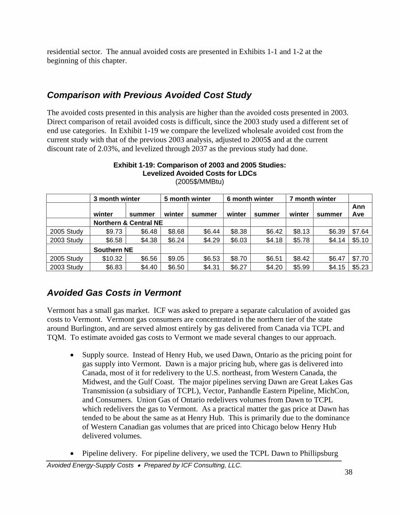
Avoided Energy-Supply Costs • Prepared by ICF Consulting, LLC.
38
residential sector. The annual avoided costs are presented in Exhibits 1-1 and 1-2 at the beginning of this chapter.
Comparison with Previous Avoided Cost Study
The avoided costs presented in this analysis are higher than the avoided costs presented in 2003. Direct comparison of retail avoided costs is difficult, since the 2003 study used a different set of end use categories. In Exhibit 1-19 we compare the levelized wholesale avoided cost from the current study with that of the previous 2003 analysis, adjusted to 2005$ and at the current discount rate of 2.03%, and levelized through 2037 as the previous study had done.
Exhibit 1-19: Comparison of 2003 and 2005 Studies: Levelized Avoided Costs for LDCs
(2005$/MMBtu) 3 month winter 5 month winter 6 month winter 7 month winter
winter summer winter summer winter summer winter summer Ann Ave
Northern & Central NE 2005 Study $9.73 $6.48 $8.68 $6.44 $8.38 $6.42 $8.13 $6.39 $7.64 2003 Study $6.58 $4.38 $6.24 $4.29 $6.03 $4.18 $5.78 $4.14 $5.10 Southern NE 2005 Study $10.32 $6.56 $9.05 $6.53 $8.70 $6.51 $8.42 $6.47 $7.70 2003 Study $6.83 $4.40 $6.50 $4.31 $6.27 $4.20 $5.99 $4.15 $5.23
Avoided Gas Costs in Vermont
Vermont has a small gas market. ICF was asked to prepare a separate calculation of avoided gas costs to Vermont. Vermont gas consumers are concentrated in the northern tier of the state around Burlington, and are served almost entirely by gas delivered from Canada via TCPL and TQM. To estimate avoided gas costs to Vermont we made several changes to our approach.
• Supply source. Instead of Henry Hub, we used Dawn, Ontario as the pricing point for gas supply into Vermont. Dawn is a major pricing hub, where gas is delivered into Canada, most of it for redelivery to the U.S. northeast, from Western Canada, the Midwest, and the Gulf Coast. The major pipelines serving Dawn are Great Lakes Gas Transmission (a subsidiary of TCPL), Vector, Panhandle Eastern Pipeline, MichCon, and Consumers. Union Gas of Ontario redelivers volumes from Dawn to TCPL which redelivers the gas to Vermont. As a practical matter the gas price at Dawn has tended to be about the same as at Henry Hub. This is primarily due to the dominance of Western Canadian gas volumes that are priced into Chicago below Henry Hub delivered volumes.
• Pipeline delivery. For pipeline delivery, we used the TCPL Dawn to Phillipsburg
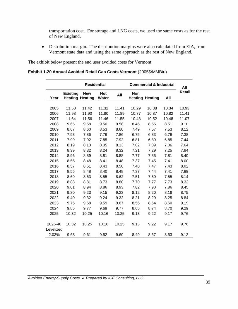
Avoided Energy-Supply Costs • Prepared by ICF Consulting, LLC.
39
transportation cost. For storage and LNG costs, we used the same costs as for the rest of New England.
• Distribution margin. The distribution margins were also calculated from EIA, from Vermont state data and using the same approach as the rest of New England.
The exhibit below present the end user avoided costs for Vermont.
Exhibit 1-20 Annual Avoided Retail Gas Costs Vermont (2005$/MMBtu)
Residential Commercial & Industrial
Year Existing Heating
New Heating
Hot Water
All Non Heating Heating All
All Retail
2005 11.50 11.42 11.32 11.41 10.29 10.38 10.34 10.93 2006 11.98 11.90 11.80 11.89 10.77 10.87 10.82 11.41 2007 11.64 11.56 11.46 11.55 10.43 10.52 10.48 11.07 2008 9.65 9.58 9.50 9.58 8.46 8.55 8.51 9.10 2009 8.67 8.60 8.53 8.60 7.49 7.57 7.53 8.12 2010 7.93 7.86 7.79 7.86 6.75 6.83 6.79 7.38 2011 7.99 7.92 7.85 7.92 6.81 6.89 6.85 7.44 2012 8.19 8.13 8.05 8.13 7.02 7.09 7.06 7.64 2013 8.39 8.32 8.24 8.32 7.21 7.29 7.25 7.84 2014 8.96 8.89 8.81 8.88 7.77 7.85 7.81 8.40 2015 8.55 8.48 8.41 8.48 7.37 7.45 7.41 8.00 2016 8.57 8.51 8.43 8.50 7.40 7.47 7.43 8.02 2017 8.55 8.48 8.40 8.48 7.37 7.44 7.41 7.99 2018 8.69 8.63 8.55 8.62 7.51 7.59 7.55 8.14 2019 8.88 8.81 8.73 8.80 7.70 7.77 7.73 8.32 2020 9.01 8.94 8.86 8.93 7.82 7.90 7.86 8.45 2021 9.30 9.23 9.15 9.23 8.12 8.20 8.16 8.75 2022 9.40 9.32 9.24 9.32 8.21 8.29 8.25 8.84 2023 9.75 9.68 9.59 9.67 8.56 8.64 8.60 9.19 2024 9.85 9.77 9.69 9.77 8.65 8.74 8.70 9.29 2025 10.32 10.25 10.16 10.25 9.13 9.22 9.17 9.76
2026-40 10.32 10.25 10.16 10.25 9.13 9.22 9.17 9.76 Levelized
2.03% 9.68 9.61 9.52 9.60 8.49 8.57 8.53 9.12
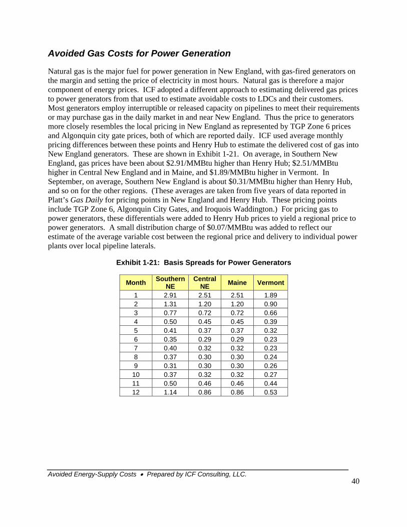
Avoided Energy-Supply Costs • Prepared by ICF Consulting, LLC.
40
Avoided Gas Costs for Power Generation
Natural gas is the major fuel for power generation in New England, with gas-fired generators on the margin and setting the price of electricity in most hours. Natural gas is therefore a major component of energy prices. ICF adopted a different approach to estimating delivered gas prices to power generators from that used to estimate avoidable costs to LDCs and their customers. Most generators employ interruptible or released capacity on pipelines to meet their requirements or may purchase gas in the daily market in and near New England. Thus the price to generators more closely resembles the local pricing in New England as represented by TGP Zone 6 prices and Algonquin city gate prices, both of which are reported daily. ICF used average monthly pricing differences between these points and Henry Hub to estimate the delivered cost of gas into New England generators. These are shown in Exhibit 1-21. On average, in Southern New England, gas prices have been about $2.91/MMBtu higher than Henry Hub; $2.51/MMBtu higher in Central New England and in Maine, and $1.89/MMBtu higher in Vermont. In September, on average, Southern New England is about $0.31/MMBtu higher than Henry Hub, and so on for the other regions. (These averages are taken from five years of data reported in Platt’s Gas Daily for pricing points in New England and Henry Hub. These pricing points include TGP Zone 6, Algonquin City Gates, and Iroquois Waddington.) For pricing gas to power generators, these differentials were added to Henry Hub prices to yield a regional price to power generators. A small distribution charge of $0.07/MMBtu was added to reflect our estimate of the average variable cost between the regional price and delivery to individual power plants over local pipeline laterals.
Exhibit 1-21: Basis Spreads for Power Generators
Month Southern NE
Central NE Maine Vermont
1 2.91 2.51 2.51 1.89 2 1.31 1.20 1.20 0.90 3 0.77 0.72 0.72 0.66 4 0.50 0.45 0.45 0.39 5 0.41 0.37 0.37 0.32 6 0.35 0.29 0.29 0.23 7 0.40 0.32 0.32 0.23 8 0.37 0.30 0.30 0.24 9 0.31 0.30 0.30 0.26
10 0.37 0.32 0.32 0.27 11 0.50 0.46 0.46 0.44 12 1.14 0.86 0.86 0.53
Avoided Energy-Supply Costs • Prepared by ICF Consulting, LLC.
41
Chapter Two: Wholesale Electricity Price Modeling Methodology, New England Power Market and Key Assumptions Overview
Introduction
The largest component of retail avoidable electricity costs is the price for firm (energy plus capacity) power available from the generation or wholesale sector. The marginal energy price plus the marginal capacity price captures this component. In order to forecast marginal energy and capacity prices for this avoided cost study, ICF relied on a fundamentals based computer simulation model, IPM®. This Chapter will focus on the methodology and assumptions driving the forecasts of the wholesale power market prices. For purposes of modeling the energy and capacity clearing prices, the analysis assumes that the markets will be perfectly competitive. Actual markets may tend to have some deviation from perfect competition which could results in higher market pricing. The remaining key components of retail avoidable electricity costs include out-of-market system reliability or congestion charges, transmission and distribution capacity costs, and distribution losses. An overview of out-of-market reliability and congestion costs are discussed in this chapter. Transmission and distribution elements will be addressed in Chapters 3 and 5. Additional retail service costs (such as customer support) are not considered to be directly avoidable as discussed in Chapter 3.
This Chapter is organized in three key sections. First we provide an overview of the modeling methodology. A detailed description of the New England wholesale power market follows, and includes a discussion of the New England LICAP (locational installed capacity) demand curves. This chapter concludes with a presentation of the key driving assumptions of the wholesale energy and capacity price forecasts.
Wholesale Price Forecasting Methodology
Energy Pricing
Competitive wholesale or spot electric energy prices are determined on an hourly basis by the intersection of supply (the available generating resources) and demand. A simplified example of this is shown in Exhibit 2-1. In each hour, the prevailing spot price of electric energy will be approximated by the short run marginal cost of production of the most expensive unit operating
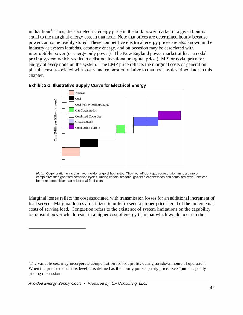
Avoided Energy-Supply Costs • Prepared by ICF Consulting, LLC.
42
in that hour1. Thus, the spot electric energy price in the bulk power market in a given hour is equal to the marginal energy cost in that hour. Note that prices are determined hourly because power cannot be readily stored. These competitive electrical energy prices are also known in the industry as system lambdas, economy energy, and on occasion may be associated with interruptible power (or energy only power). The New England power market utilizes a nodal pricing system which results in a distinct locational marginal price (LMP) or nodal price for energy at every node on the system. The LMP price reflects the marginal costs of generation plus the cost associated with losses and congestion relative to that node as described later in this chapter.
Exhibit 2-1: Illustrative Supply Curve for Electrical Energy
Marginal losses reflect the cost associated with transmission losses for an additional increment of load served. Marginal losses are utilized in order to send a proper price signal of the incremental costs of serving load. Congestion refers to the existence of system limitations on the capability to transmit power which result in a higher cost of energy than that which would occur in the
1The variable cost may incorporate compensation for lost profits during turndown hours of operation. When the price exceeds this level, it is defined as the hourly pure capacity price. See “pure” capacity pricing discussion.
Nuclear
Coal
Coal with Wheeling Charge
Gas Cogeneration
Oil/Gas Steam
Combustion Turbine
Fall Weekend Morning Summer Weekday10 AM
Cos
t (M
ills p
er K
ilow
att-h
our)
Combined Cycle Gas
Generation Supply (MW)Note: Cogeneration units can have a wide range of heat rates. The most efficient gas cogeneration units are more competitive than gas-fired combined cycles. During certain seasons, gas-fired cogeneration and combined cycle units can be more competitive than select coal-fired units.
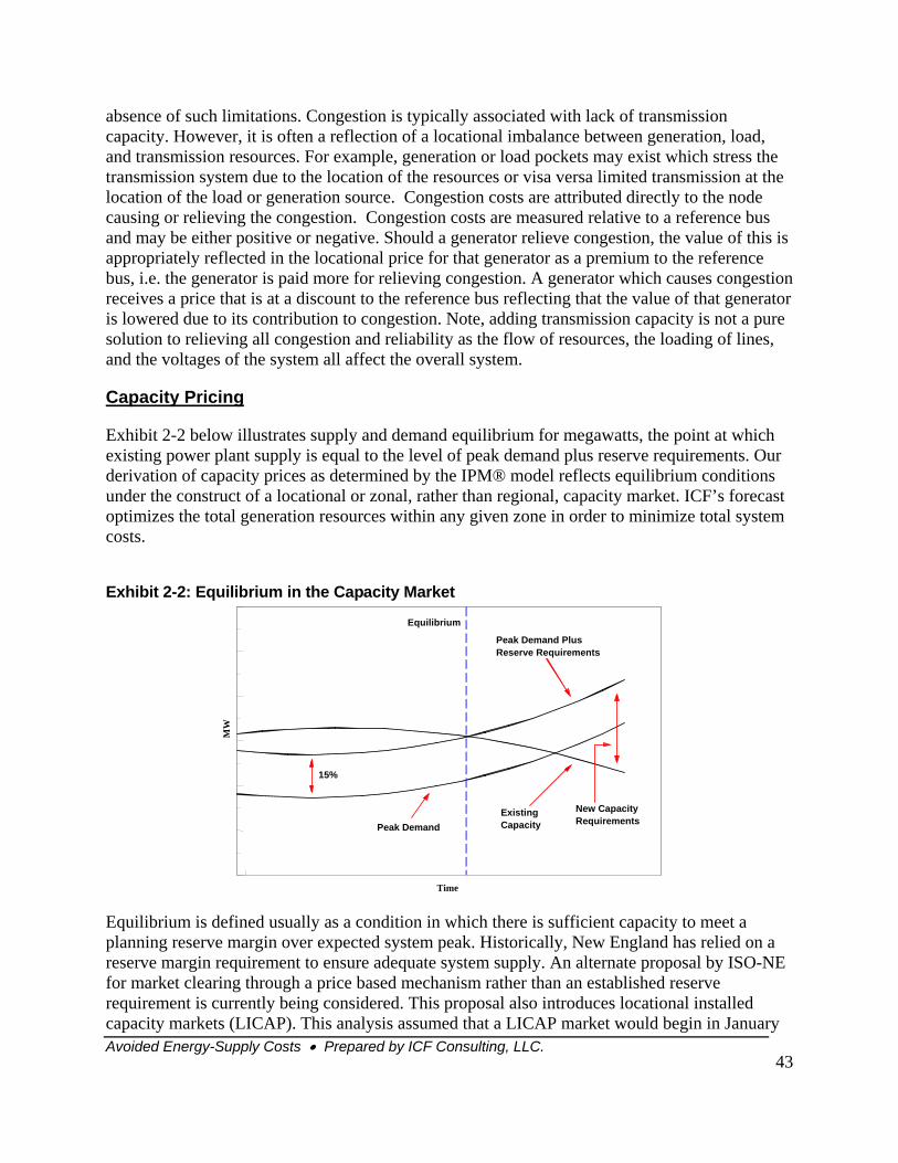
Avoided Energy-Supply Costs • Prepared by ICF Consulting, LLC.
43
absence of such limitations. Congestion is typically associated with lack of transmission capacity. However, it is often a reflection of a locational imbalance between generation, load, and transmission resources. For example, generation or load pockets may exist which stress the transmission system due to the location of the resources or visa versa limited transmission at the location of the load or generation source. Congestion costs are attributed directly to the node causing or relieving the congestion. Congestion costs are measured relative to a reference bus and may be either positive or negative. Should a generator relieve congestion, the value of this is appropriately reflected in the locational price for that generator as a premium to the reference bus, i.e. the generator is paid more for relieving congestion. A generator which causes congestion receives a price that is at a discount to the reference bus reflecting that the value of that generator is lowered due to its contribution to congestion. Note, adding transmission capacity is not a pure solution to relieving all congestion and reliability as the flow of resources, the loading of lines, and the voltages of the system all affect the overall system.
Capacity Pricing
Exhibit 2-2 below illustrates supply and demand equilibrium for megawatts, the point at which existing power plant supply is equal to the level of peak demand plus reserve requirements. Our derivation of capacity prices as determined by the IPM® model reflects equilibrium conditions under the construct of a locational or zonal, rather than regional, capacity market. ICF’s forecast optimizes the total generation resources within any given zone in order to minimize total system costs.
Exhibit 2-2: Equilibrium in the Capacity Market
Equilibrium is defined usually as a condition in which there is sufficient capacity to meet a planning reserve margin over expected system peak. Historically, New England has relied on a reserve margin requirement to ensure adequate system supply. An alternate proposal by ISO-NE for market clearing through a price based mechanism rather than an established reserve requirement is currently being considered. This proposal also introduces locational installed capacity markets (LICAP). This analysis assumed that a LICAP market would begin in January
Time
MW
Peak Demand PlusReserve Requirements
Existing Capacity
New CapacityRequirementsPeak Demand
15%
Equilibrium
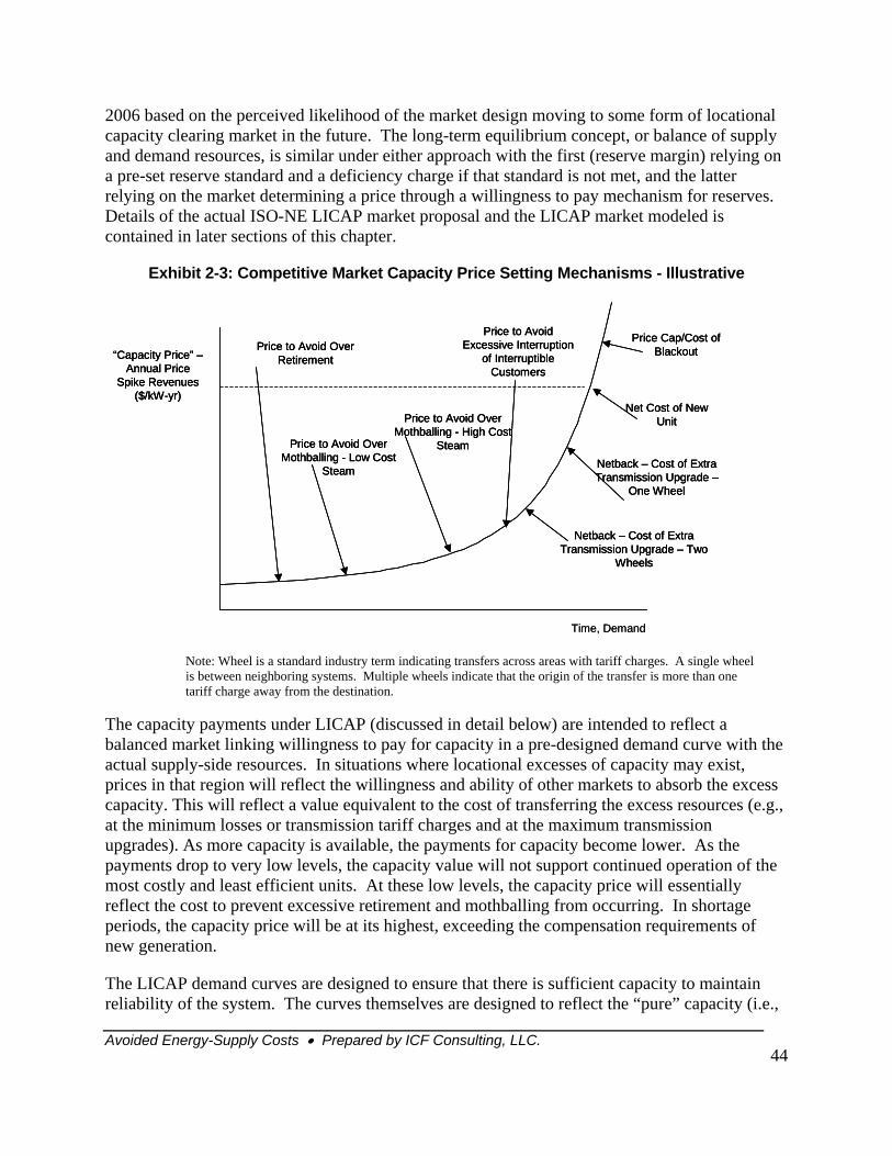
Avoided Energy-Supply Costs • Prepared by ICF Consulting, LLC.
44
2006 based on the perceived likelihood of the market design moving to some form of locational capacity clearing market in the future. The long-term equilibrium concept, or balance of supply and demand resources, is similar under either approach with the first (reserve margin) relying on a pre-set reserve standard and a deficiency charge if that standard is not met, and the latter relying on the market determining a price through a willingness to pay mechanism for reserves. Details of the actual ISO-NE LICAP market proposal and the LICAP market modeled is contained in later sections of this chapter.
Exhibit 2-3: Competitive Market Capacity Price Setting Mechanisms - Illustrative
The capacity payments under LICAP (discussed in detail below) are intended to reflect a balanced market linking willingness to pay for capacity in a pre-designed demand curve with the actual supply-side resources. In situations where locational excesses of capacity may exist, prices in that region will reflect the willingness and ability of other markets to absorb the excess capacity. This will reflect a value equivalent to the cost of transferring the excess resources (e.g., at the minimum losses or transmission tariff charges and at the maximum transmission upgrades). As more capacity is available, the payments for capacity become lower. As the payments drop to very low levels, the capacity value will not support continued operation of the most costly and least efficient units. At these low levels, the capacity price will essentially reflect the cost to prevent excessive retirement and mothballing from occurring. In shortage periods, the capacity price will be at its highest, exceeding the compensation requirements of new generation.
The LICAP demand curves are designed to ensure that there is sufficient capacity to maintain reliability of the system. The curves themselves are designed to reflect the “pure” capacity (i.e.,
“Capacity Price” –Annual Price
Spike Revenues($/kW-yr)
Price to Avoid Over Retirement
Price to Avoid Over Mothballing - Low Cost
Steam
Price to Avoid Over Mothballing - High Cost
Steam
Price to Avoid Excessive Interruption
of Interruptible Customers
Price Cap/Cost of Blackout
Net Cost of New Unit
Netback – Cost of Extra Transmission Upgrade –
One Wheel
Netback – Cost of Extra Transmission Upgrade – Two
Wheels
Time, Demand
“Capacity Price” –Annual Price
Spike Revenues($/kW-yr)
Price to Avoid Over Retirement
Price to Avoid Over Mothballing - Low Cost
Steam
Price to Avoid Over Mothballing - High Cost
Steam
Price to Avoid Excessive Interruption
of Interruptible Customers
Price Cap/Cost of Blackout
Net Cost of New Unit
Netback – Cost of Extra Transmission Upgrade –
One Wheel
Netback – Cost of Extra Transmission Upgrade – Two
Wheels
Time, Demand
Note: Wheel is a standard industry term indicating transfers across areas with tariff charges. A single wheel is between neighboring systems. Multiple wheels indicate that the origin of the transfer is more than one tariff charge away from the destination.
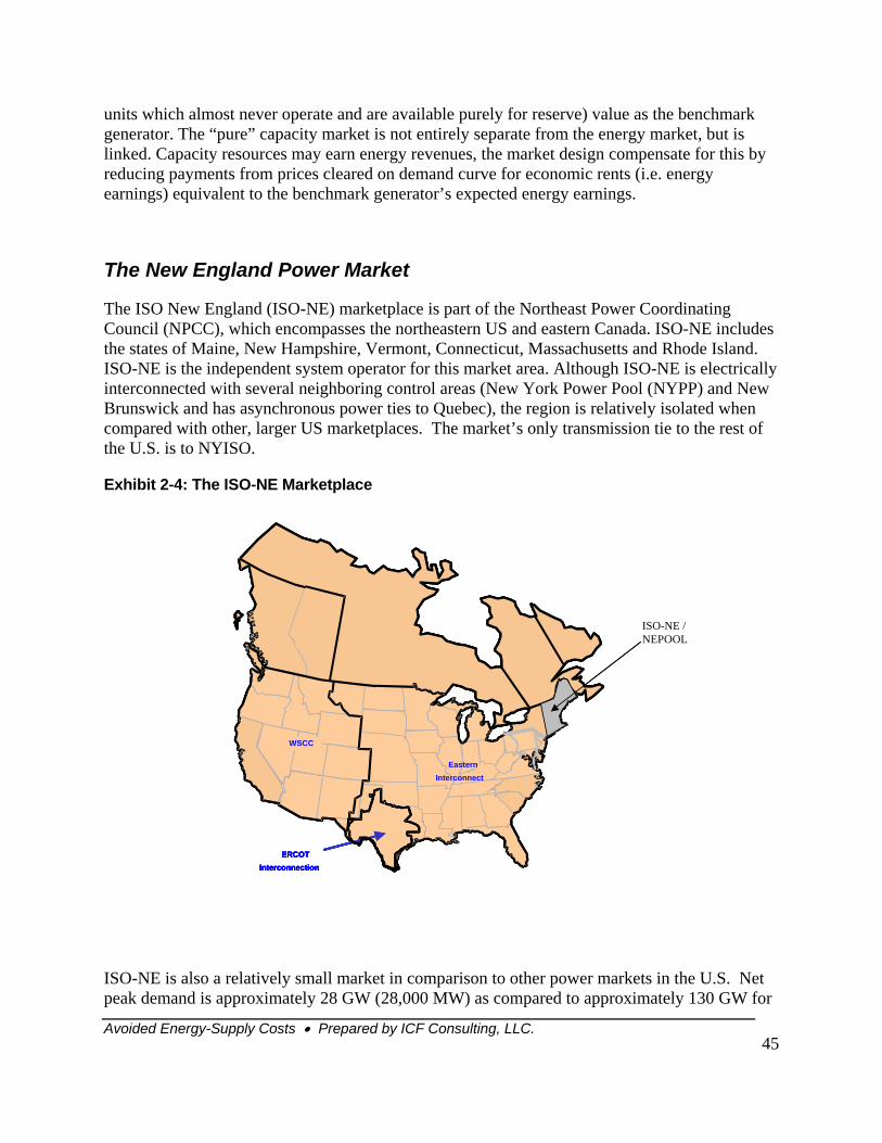
Avoided Energy-Supply Costs • Prepared by ICF Consulting, LLC.
45
units which almost never operate and are available purely for reserve) value as the benchmark generator. The “pure” capacity market is not entirely separate from the energy market, but is linked. Capacity resources may earn energy revenues, the market design compensate for this by reducing payments from prices cleared on demand curve for economic rents (i.e. energy earnings) equivalent to the benchmark generator’s expected energy earnings.
The New England Power Market
The ISO New England (ISO-NE) marketplace is part of the Northeast Power Coordinating Council (NPCC), which encompasses the northeastern US and eastern Canada. ISO-NE includes the states of Maine, New Hampshire, Vermont, Connecticut, Massachusetts and Rhode Island. ISO-NE is the independent system operator for this market area. Although ISO-NE is electrically interconnected with several neighboring control areas (New York Power Pool (NYPP) and New Brunswick and has asynchronous power ties to Quebec), the region is relatively isolated when compared with other, larger US marketplaces. The market’s only transmission tie to the rest of the U.S. is to NYISO.
Exhibit 2-4: The ISO-NE Marketplace
ISO-NE is also a relatively small market in comparison to other power markets in the U.S. Net peak demand is approximately 28 GW (28,000 MW) as compared to approximately 130 GW for
ERCOTInterconnection
WSCC
EasternInterconnect
ERCOTInterconnection
WSCC
EasternInterconnect
ERCOTInterconnection
WSCC
EasternInterconnect
ERCOTInterconnection
WSCC
EasternInterconnect
ISO-NE / NEPOOL
Avoided Energy-Supply Costs • Prepared by ICF Consulting, LLC.
46
PJM (PJM spans Pennsylvania, New Jersey, Maryland, Delaware, parts of Ohio, and parts of Illinois. FERC has been restructuring the ISO-NE market due to concerns that suppliers have market power. These concerns are fed by the fact that ISO-NE is relatively small and also because it is isolated from other markets as described above. This concern has also been fed by the existence of transmission constraints that create sub-markets within ISO-NE. As these concerns were not fully envisioned in the original ISO-NE market design, FERC and ISO-NE have spent the last few years reformulating the markets.
ISO-NE Markets Are Continually Undergoing Change
New England has a long history of multi-utility coordination which influenced ISO-NE’s development. Formed in 1971, the New England Power Pool (NEPOOL) was a voluntary association of electric power industry participants in New England. NEPOOL established a single regional network to direct the operations of the major generating and transmission (bulk power system) facilities in the region.
Under this structure, NEPOOL distributed transmission congestion costs among the utilities via payment of out-of-merit dispatch costs as the operators worked around transmission problems by changing plant utilization patterns to include higher cost but more strategically located generators. Under the regulated market structure, numerous nuclear power plants serving broad-based customers and accompanying (though separately proposed) large transmission projects which decreased congestion had been built in the NEPOOL administered market.
NEPOOL’s existence contributed to the quick establishment of a multi-utility marketplace when FERC Order 888 established open and comparable access to transmission. ISO New England (ISO-NE) was established as a not-for-profit, private corporation in 1997. The organization immediately assumed responsibility for managing the New England region's electric bulk power generation and transmission systems and administering the region's open access transmission tariff. ISO-NE, also known as RTO NE (RTO – Regional Transmission Organization) is in many respects in the forefront of U.S. deregulation of the electric power industry. Nearly all electric utilities in New England have already fully divested their generation. Most New England states have created the potential for end-users to purchase power from other suppliers. ISO-NE power plants and the associated high voltage electricity transmission grids are regulated directly by FERC. There are practically no vertically integrated, traditional utilities and no major new rate-based regulated power plants have been built in New England in more than fifteen years. ISO-NE operates a power market for buyers (LSEs – Load Serving Entities) and generators, and coordinates grid operation.
Starting on May 1, 1999, ISO New England has been administering the wholesale electricity marketplace for the region subject to FERC regulation. Six electricity products were originally established for sale and purchase by market participants:
• Energy • ICAP (Installed Capability Market), • 10-minute spinning reserves, • 10-minute non-spinning reserves,
Avoided Energy-Supply Costs • Prepared by ICF Consulting, LLC.
47
• 30-minute operating reserves, and • Automatic generation control (AGC).
This marketplace adopted many of the structures of NEPOOL including a single New England energy market. By end-1999, New England was the only one of the three Northeast Independent System Operators (New York ISO and PJM being the other two) without a location-based energy market. That is, only ISO-NE had a single electrical energy price for all buyers and sellers regardless of location and the generator’s impact on grid congestion. Congestion derived re-dispatch costs were paid by the ISO and passed through to end-users. However, with the anticipation of deregulation and the transition to the ISO-NE market structure, the joint transmission projects of earlier years stopped. As electricity demand continued to grow, transmission congestion costs increased and internal transmission constraints began to contribute to load and generation pockets.
Under FERC pressure, this system was replaced with a location based pricing system for energy. Since March 1, 2003, the New England ISO began pricing energy using a locational marginal pricing (LMP) scheme similar to those used in New York, MISO (Midwest Independent System Operator), and PJM markets. Under the LMP pricing scheme, nodal prices that are received as payment to generators are lower for those generators contributing to congestion and higher for those reducing congestion than they otherwise would be if there were no congestion. Similarly, the price signals indicate the investment needed in generation itself. If a new power plant were to locate in an LMP market, the developer would consider the costs of transmission upgrades necessary to allow the plant to meet deliverability standards as part of the development costs of the project. Absent the LMP design, the generation owner would have received the market price regardless of its impact on congestion.
Another early feature adopted by ISO-NE was a separate installed capacity market. This was an outgrowth of NEPOOL’s separation of energy and capacity products. On the energy side, NEPOOL centrally dispatched for energy in its power exchange. On the capacity side, NEPOOL addressed capacity via deficiency penalties for utilities without adequate reserves. In this respect, ISO-NE was similar to the other two Northeastern U.S. tight power pools (PJM and New York) which also separated the two products. Recognizing transmission limitations within its electrical grid, New York was the first of the three marketplaces to advance the concept of a locational capacity market. New England and PJM are now both pursuing locational capacity markets.
ISO-NE has significant internal transmission problems even within its small footprint. This has contributed to concerns that generation owners have market power. Unlike New York which based its original design on internal transmission problems and market power, the original ISO-NE capacity market design failed to differentiate sub-markets associated with transmission constraints and as such did not address market power mitigation fully. ISO-NE has needed to undergo a re-design process to address these problems. This process has been ongoing for a number of years; the FERC docket related to the capacity market redesign matters has extended from 2001 to 2005. As a temporary measure to assure that capacity receive adequate payment to reliably serve the market, ISO-NE has adopted a quasi re-regulation process known as Reliability Must-Run (RMR) which has become especially important in load pockets
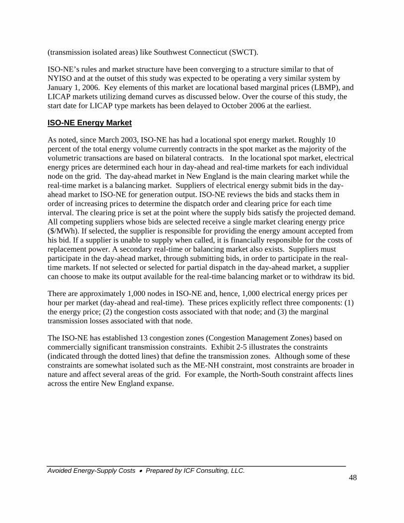
Avoided Energy-Supply Costs • Prepared by ICF Consulting, LLC.
48
(transmission isolated areas) like Southwest Connecticut (SWCT).
ISO-NE’s rules and market structure have been converging to a structure similar to that of NYISO and at the outset of this study was expected to be operating a very similar system by January 1, 2006. Key elements of this market are locational based marginal prices (LBMP), and LICAP markets utilizing demand curves as discussed below. Over the course of this study, the start date for LICAP type markets has been delayed to October 2006 at the earliest.
ISO-NE Energy Market
As noted, since March 2003, ISO-NE has had a locational spot energy market. Roughly 10 percent of the total energy volume currently contracts in the spot market as the majority of the volumetric transactions are based on bilateral contracts. In the locational spot market, electrical energy prices are determined each hour in day-ahead and real-time markets for each individual node on the grid. The day-ahead market in New England is the main clearing market while the real-time market is a balancing market. Suppliers of electrical energy submit bids in the day-ahead market to ISO-NE for generation output. ISO-NE reviews the bids and stacks them in order of increasing prices to determine the dispatch order and clearing price for each time interval. The clearing price is set at the point where the supply bids satisfy the projected demand. All competing suppliers whose bids are selected receive a single market clearing energy price ($/MWh). If selected, the supplier is responsible for providing the energy amount accepted from his bid. If a supplier is unable to supply when called, it is financially responsible for the costs of replacement power. A secondary real-time or balancing market also exists. Suppliers must participate in the day-ahead market, through submitting bids, in order to participate in the real-time markets. If not selected or selected for partial dispatch in the day-ahead market, a supplier can choose to make its output available for the real-time balancing market or to withdraw its bid.
There are approximately 1,000 nodes in ISO-NE and, hence, 1,000 electrical energy prices per hour per market (day-ahead and real-time). These prices explicitly reflect three components: (1) the energy price; (2) the congestion costs associated with that node; and (3) the marginal transmission losses associated with that node.
The ISO-NE has established 13 congestion zones (Congestion Management Zones) based on commercially significant transmission constraints. Exhibit 2-5 illustrates the constraints (indicated through the dotted lines) that define the transmission zones. Although some of these constraints are somewhat isolated such as the ME-NH constraint, most constraints are broader in nature and affect several areas of the grid. For example, the North-South constraint affects lines across the entire New England expanse.
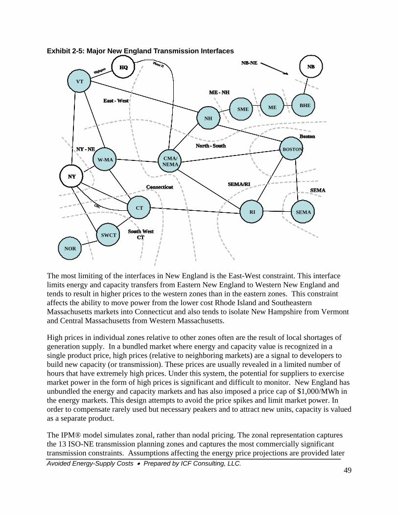
Avoided Energy-Supply Costs • Prepared by ICF Consulting, LLC.
49
Exhibit 2-5: Major New England Transmission Interfaces
rface limits energy and capacity transfers from Eastern New England to Western New England and tends to result in higher prices to the western zones than in the eastern zones. This constraint affects the ability to move power from the lower cost Rhode Island and Southeastern Massachusetts markets into Connecticut and also tends to isolate New Hampshire from Vermont and Central Massachusetts from Western Massachusetts.
High prices in individual zones relative to other zones often are the result of local shortages of generation supply. In a bundled market where energy and capacity value is recognized in a single product price, high prices (relative to neighboring markets) are a signal to developers to build new capacity (or transmission). These prices are usually revealed in a limited number of hours that have extremely high prices. Under this system, the potential for suppliers to exercise market power in the form of high prices is significant and difficult to monitor. New England has unbundled the energy and capacity markets and has also imposed a price cap of $1,000/MWh in the energy markets. This design attempts to avoid the price spikes and limit market power. In order to compensate rarely used but necessary peakers and to attract new units, capacity is valued as a separate product.
The IPM® model simulates zonal, rather than nodal pricing. The zonal representation captures the 13 ISO-NE transmission planning zones and captures the most commercially significant transmission constraints. Assumptions affecting the energy price projections are provided later
The most limiting of the interfaces in New England is the East-West constraint. This inte
BHE
NH
ME
BOSTON
RI SEMACT
SWCT
CMA/NEMA
W-MA
VT
NY
East East -- WestWestME ME -- NHNH
North North -- SouthSouth
BostonBoston
SEMA/RISEMA/RISEMASEMA
NY NY -- NENE
South WestSouth WestCTCT
ConnecticutConnecticut
-HQ
HighgateHighgate
Phase IIPhase II
CSCCSC
NB
NH
SME
BOSTON
RI SEMACT
SWCT
CMA/NEMA
W-MA
VT
NY
East East -- WestWestME ME -- NHNH
North North -- SouthSouth
BostonBoston
SEMA/RISEMA/RISEMASEMA
NY NY -- NENE
South WestSouth WestCTCT
ConnecticutConnecticut
NB-NE HQ
HighgateHighgate
Phase IIPhase II
CSCCSC
NOR
ME BHE
NH
ME
BOSTON
RI SEMACT
SWCT
CMA/NEMA
W-MA
VT
NY
East East -- WestWestME ME -- NHNH
North North -- SouthSouth
BostonBoston
SEMA/RISEMA/RISEMASEMA
NY NY -- NENE
South WestSouth WestCTCT
ConnecticutConnecticut
-HQ
HighgateHighgate
Phase IIPhase II
CSCCSC
NB
NH
SME
BOSTON
RI SEMACT
SWCT
CMA/NEMA
W-MA
VT
NY
East East -- WestWestME ME -- NHNH
North North -- SouthSouth
BostonBoston
SEMA/RISEMA/RISEMASEMA
NY NY -- NENE
South WestSouth WestCTCT
ConnecticutConnecticut
NB-NE HQ
HighgateHighgate
Phase IIPhase II
CSCCSC
NOR
BHE
NH
ME
BOSTON
RI SEMACT
SWCT
CMA/NEMA
W-MA
VT
NY
East East -- WestWestME ME -- NHNH
North North -- SouthSouth
BostonBoston
SEMA/RISEMA/RISEMASEMA
NY NY -- NENE
South WestSouth WestCTCT
ConnecticutConnecticut
-HQ
HighgateHighgate
Phase IIPhase II
CSCCSC
NB
NH
SME
BOSTON
RI SEMACT
SWCT
CMA/NEMA
W-MA
VT
NY
East East -- WestWestME ME -- NHNH
North North -- SouthSouth
BostonBoston
SEMA/RISEMA/RISEMASEMA
NY NY -- NENE
South WestSouth WestCTCT
ConnecticutConnecticut
NB-NE HQ
HighgateHighgate
Phase IIPhase II
CSCCSC
NOR
ME
Avoided Energy-Supply Costs • Prepared by ICF Consulting, LLC.
50
in this chapter.
ISO-NE Installed Capacity Market
As mentioned, an ICAP market has existed in New England since the ISO-NE began operating the system. There have been capacity market precursors such as the NEPOOL deficiency charges for lack of reserve capacity that predate the ISO-NE current market. These deficiency charges were set based on the cost of peaking capacity and provided incentives to utilities to have enough supply to ensure generation adequacy.
Capacity markets are designed to shift scarcity value (the value for limited resources) for capacity from energy markets to a separate market. Under FERC regulation, and based on ISO-NE’s experience with shortages in the late 1990s, increased emphasis was placed on having separate energy and capacity markets to facilitate attention on market power and prevent excessive price volatility. This was coincident with increasingly sophisticated treatment of transmission effects. However, separation of energy and capacity requires both markets to work properly if revenue is to be sufficient to allow for reliability while not being too high given FERC’s market power concerns. This increases regulatory requirements, especially since FERC’s efforts to develop a Standard Market Design (SMD) floundered during the 2001-2003 period. In the aftermath of the SMD effort, regulators needed to develop region by region solutions even while trying to decrease differences to facilitate integration.
The ISO-NE established target reliability levels reflects three factors: (1) customer willingness to pay to avoid a black-out is very high, and hence, the goal is to provide customers very high reliability levels that limit expected load shedding (i.e., rolling black-outs) to one day in ten years (0.99973 availability for power supply), (2) industry convention to estimate expected peak demand based on average weather conditions (as opposed to worst day in 100 years, etc.), and hence, one-half of the time peak electricity demand exceeds the expected level applying stress to the system, and (3) industry convention to estimate installed capacity at maximum output even though it is extremely rare that all units are available at maximum output.
Several features of the original ICAP Market include:
• Monthly Bidding – The original ICAP market was designed to settle prices on a monthly basis based on bids for the uncommitted capacity of the generator’s participating in the ISO-NE. This bidding gives sellers the opportunity to raise bids above costs and potentially to exercise market power. This is especially true in small isolated markets. Since its inception, the ICAP market pricing has been a focus of FERC attention both in terms of reliability and market power.
• Seasonal Allocations – ISO-NE calculates the Summer Capability Period and Winter Capability Period Installed Capacity Requirements each year. The ISO-NE then converts the Installed Capacity Requirements into Unforced Capacity (UCAP) Requirements for the entire ISO-NE Control Area and allocates the

Avoided Energy-Supply Costs • Prepared by ICF Consulting, LLC.
51
requirements to Participants based upon their customers’ contributions to the previous calendar year’s ISO-NE Control Area coincident peak load. The UCAP amount represents the capacity that is shown to be available when called on or the installed capacity after accounting for the forced outage rate. Thus, every participant must shoulder its share of the reliability burden, i.e., the cost of keeping reserves.
• Load Shifting and Allocated ICAP Requirements – All LSEs (Load Serving Entities) contribute to the NEPOOL peak, and therefore are allocated a UCAP requirement based on their coincident load. The UCAP obligation for each LSE (Participant) within New England is adjusted each month to reflect changes in obligation that result from load-shifting, as well as other changes in obligation. These monthly requirements are binding with regard to the Participant’s obligation to procure UCAP for the following month. The obligation is calculated as the sum of all UCAP Peak Contributions for all customers served by that Participant, divided by the sum of all contributions. Participants may use this market to procure supplies to satisfy the Unforced Capacity requirement in advance of the next obligation month. Participant compliance may also include bilateral contracts, capacity credits or ownership of qualified resources.
• Deficiency Charge – Participants must demonstrate adequate supplies to ISO-NE; if not demonstrated, ISO-NE has the authority to impose sanctions on the Participant, or submit deficiency bids on behalf of the Participant. Under the Deficiency Auction, Participants with excess UCAP are required to offer or accept a $0.00 bid if they do not offer. Offers in the auction are capped at Deficiency Charge of $6.66/kW-month.
Historical ISO-NE Installed Capacity Market Failed to Compensate Generators
After its opening in April 1998, the ICAP market prices where at $0/kW-month for all but 3 months of the first 21 months of operation (through December 1999) (see Exhibit 2-6). For the 3 months experiencing prices, the market cleared at an average price of $0.67/kW-month.
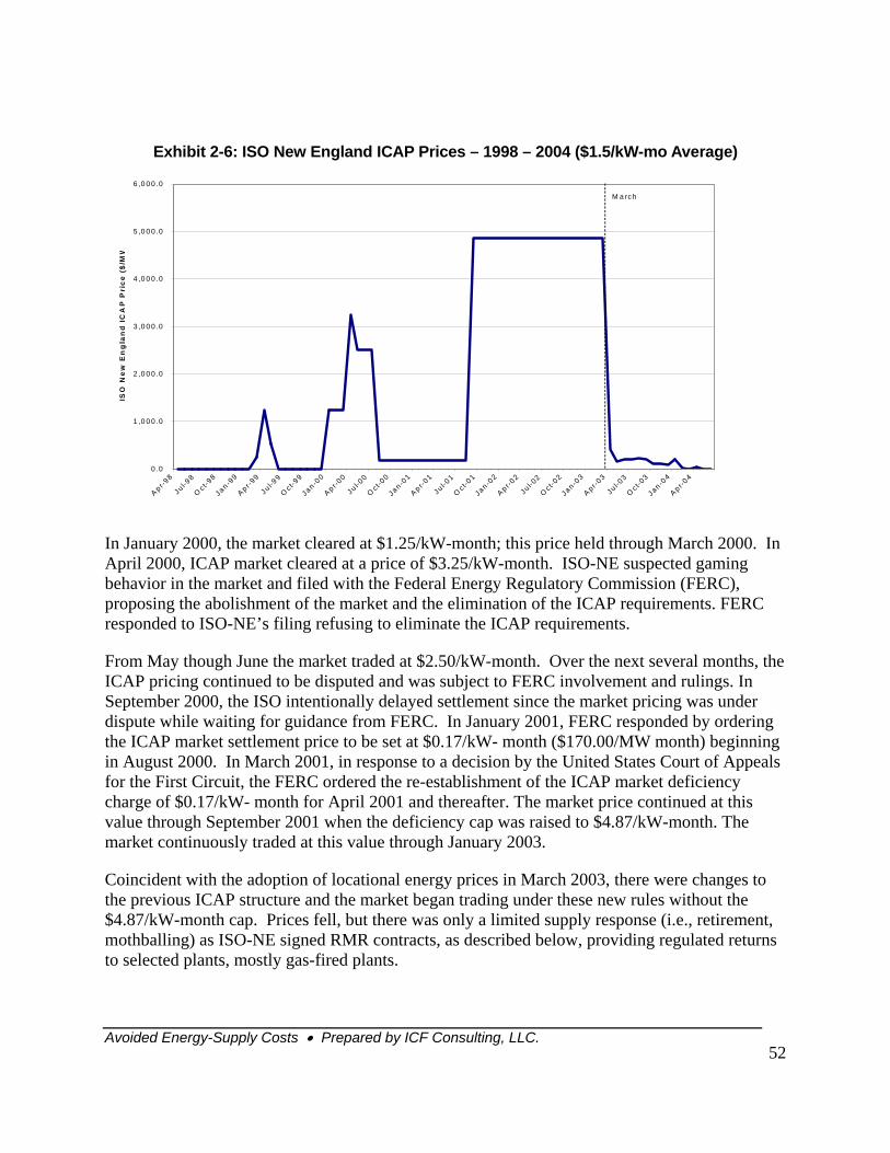
Avoided Energy-Supply Costs • Prepared by ICF Consulting, LLC.
52
Exhibit 2-6: ISO New England ICAP Prices – 1998 – 2004 ($1.5/kW-mo Average)
In January 2000, the market cleared at $1.25/kW-month; this price held through March 2000. In April 2000, ICAP market cleared at a price of $3.25/kW-month. ISO-NE suspected gaming behavior in the market and filed with the Federal Energy Regulatory Commission (FERC), proposing the abolishment of the market and the elimination of the ICAP requirements. FERC responded to ISO-NE’s filing refusing to eliminate the ICAP requirements.
From May though June the market traded at $2.50/kW-month. Over the next several months, the ICAP pricing continued to be disputed and was subject to FERC involvement and rulings. In September 2000, the ISO intentionally delayed settlement since the market pricing was under dispute while waiting for guidance from FERC. In January 2001, FERC responded by ordering the ICAP market settlement price to be set at $0.17/kW- month ($170.00/MW month) beginning in August 2000. In March 2001, in response to a decision by the United States Court of Appeals for the First Circuit, the FERC ordered the re-establishment of the ICAP market deficiency charge of $0.17/kW- month for April 2001 and thereafter. The market price continued at this value through September 2001 when the deficiency cap was raised to $4.87/kW-month. The market continuously traded at this value through January 2003.
Coincident with the adoption of locational energy prices in March 2003, there were changes to the previous ICAP structure and the market began trading under these new rules without the $4.87/kW-month cap. Prices fell, but there was only a limited supply response (i.e., retirement, mothballing) as ISO-NE signed RMR contracts, as described below, providing regulated returns to selected plants, mostly gas-fired plants.
0 .0
1 ,0 0 0 .0
2 ,0 0 0 .0
3 ,0 0 0 .0
4 ,0 0 0 .0
5 ,0 0 0 .0
6 ,0 0 0 .0
A p r-98
Ju l-98
Oc t-9
8
Jan-99
Ap r-99
Ju l-99
Oc t-9
9
Jan -00
Ap r-00
Ju l-00
Oct-0
0
Jan -01
Ap r-01
Ju l-01
Oct-0
1
Jan -02
Ap r-02
Ju l-02
Oc t-0
2
Jan -03
A p r-03
Ju l-03
Oc t-0
3
Jan -04
Ap r-04
ISO
Ne
w E
ng
lan
d I
CA
P P
ric
e (
$/M
W
M a rch
Avoided Energy-Supply Costs • Prepared by ICF Consulting, LLC.
53
Reliability Must Run (RMR)
As FERC dealt with issues related to ICAP and market power in the 2001-2003 time period, and LICAP in the 2003 to 2005 time periods, payments to gas-fired units were depressed due to low ICAP prices and emphasis on market power concerns. Since power plants have fixed costs, even short periods without coverage of fixed costs can cause them to withdraw from the market, decreasing reliability. If many plants are similarly situated, this withdrawal can be large and lead to grid collapse. This can be especially problematic in load pockets like SWCT and Boston.
In light of the extreme need to resolve this problem faster than FERC, ISO-NE under FERC regulation created a parallel system of RMR contracts designed to enable generators to recover costs not otherwise obtained in the competitive capacity market. Initially, FERC allowed payment of going forward maintenance costs under RMR contracts and directed ISO-NE to permit selected peaking units to raise their bids (Peaking Unit Safe Harbor bids or PUSH bids) in order to recover fixed and variable costs through the market, and to allow these bids to set the energy price. PUSH bids exceed marginal cost by a net annual fixed cost component which includes both sunk and going-forward costs. This temporary rule was to be in place until ISO-NE could implement a locational ICAP market. The PUSH system failed to compensate units, and, as multiple units applied for RMR, cost-of-service RMR style agreements began to effectively re-regulate portions of the grid in SWCT, Connecticut and NEMA Boston. Payments are now in the $8/kW-month range (see Exhibit 2-7). However, this system was expected to be temporary and FERC approved contracts that generally had a sunset date to match the start of the LICAP market (since 12/31/05 was the day before LICAP Planned Start, some used this date while others simply referred to the LICAP start as the expiration date).
The first RMR filings occurred in 2001, though hearings on these initial requests generally continued through 2003 when the first RMR contracts were granted. A large increase in RMR applications occurred between 2003 and 2005 as many gas-fired units could not make money during this interim period.
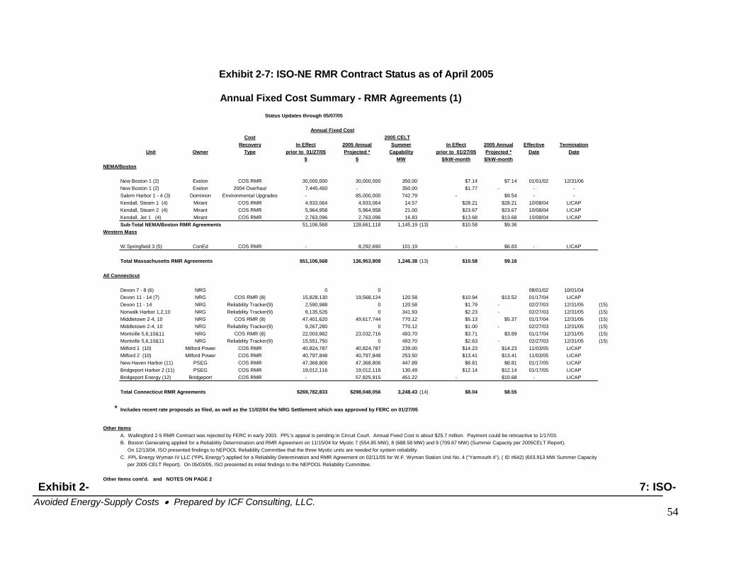
Avoided Energy-Supply Costs • Prepared by ICF Consulting, LLC.
54
Exhibit 2-7: ISO-NE RMR Contract Status as of April 2005
Exhibit 2- 7: ISO-
Annual Fixed Cost Summary - RMR Agreements (1) Status Updates through 05/07/05
Cost 2005 CELTRecovery In Effect 2005 Annual Summer In Effect 2005 Annual Effective Termination
Unit Owner Type prior to 01/27/05 Projected * Capability prior to 01/27/05 Projected * Date Date$ $ MW $/kW-month $/kW-month
NEMA/Boston
New Boston 1 (2) Exelon COS RMR 30,000,000 30,000,000 350.00 $7.14 $7.14 01/01/02 12/31/06New Boston 1 (2) Exelon 2004 Overhaul 7,445,450 - 350.00 $1.77 - - -Salem Harbor 1 - 4 (3) Dominion Environmental Upgrades - 85,000,000 742.79 - $9.54 - -Kendall, Steam 1 (4) Mirant COS RMR 4,933,064 4,933,064 14.57 $28.21 $28.21 10/08/04 LICAPKendall, Steam 2 (4) Mirant COS RMR 5,964,958 5,964,958 21.00 $23.67 $23.67 10/08/04 LICAPKendall, Jet 1 (4) Mirant COS RMR 2,763,096 2,763,096 16.83 $13.68 $13.68 10/08/04 LICAPSub-Total NEMA/Boston RMR Agreements 51,106,568 128,661,118 1,145.19 (13) $10.58 $9.36
Western Mass
W.Springfield 3 (5) ConEd COS RMR - 8,292,690 101.19 - $6.83 - LICAP
Total Massachusetts RMR Agreements $51,106,568 136,953,808 1,246.38 (13) $10.58 $9.16
All Connecticut
Devon 7 - 8 (6) NRG 0 0 08/01/02 10/01/04Devon 11 - 14 (7) NRG COS RMR (8) 15,828,130 19,568,124 120.58 $10.94 $13.52 01/17/04 LICAPDevon 11 - 14 NRG Reliability Tracker(9) 2,590,988 0 120.58 $1.79 - 02/27/03 12/31/05 (15)Norwalk Harbor 1,2,10 NRG Reliability Tracker(9) 9,135,526 0 341.93 $2.23 - 02/27/03 12/31/05 (15)Middletown 2-4, 10 NRG COS RMR (8) 47,401,620 49,617,744 770.12 $5.13 $5.37 01/17/04 12/31/05 (15)Middletown 2-4, 10 NRG Reliability Tracker(9) 9,267,280 0 770.12 $1.00 - 02/27/03 12/31/05 (15)Montville 5,6,10&11 NRG COS RMR (8) 22,003,982 23,032,716 493.70 $3.71 $3.89 01/17/04 12/31/05 (15)Montville 5,6,10&11 NRG Reliability Tracker(9) 15,551,750 0 493.70 $2.63 - 02/27/03 12/31/05 (15)Milford 1 (10) Milford Power COS RMR 40,824,787 40,824,787 239.00 $14.23 $14.23 11/03/05 LICAPMilford 2 (10) Milford Power COS RMR 40,797,848 40,797,848 253.50 $13.41 $13.41 11/03/05 LICAPNew Haven Harbor (11) PSEG COS RMR 47,368,806 47,368,806 447.89 $8.81 $8.81 01/17/05 LICAPBridgeport Harbor 2 (11) PSEG COS RMR 19,012,116 19,012,116 130.49 $12.14 $12.14 01/17/05 LICAPBridgeport Energy (12) Bridgeport COS RMR - 57,825,915 451.22 - $10.68 - LICAP
Total Connecticut RMR Agreements $269,782,833 $298,048,056 3,248.43 (14) $8.04 $8.55
* Includes recent rate proposals as filed, as well as the 11/02/04 the NRG Settlement which was approved by FERC on 01/27/05
Other ItemsA. Wallingford 2-5 RMR Contract was rejected by FERC in early 2003. PPL's appeal is pending in Circuit Court. Annual Fixed Cost is about $25.7 million. Payment could be retroactive to 1/17/03.B. Boston Generating applied for a Reliability Determination and RMR Agreement on 11/15/04 for Mystic 7 (554.85 MW), 8 (688.58 MW) and 9 (709.67 MW) (Summer Capacity per 2005CELT Report). On 12/13/04, ISO presented findings to NEPOOL Reliability Committee that the three Mystic units are needed for system reliability.C. FPL Energy Wyman IV LLC (“FPL Energy”) applied for a Reliability Determination and RMR Agreement on 02/11/05 for W.F. Wyman Station Unit No. 4 (“Yarmouth 4”), ( ID #642) (603.913 MW Summer Capacity per 2005 CELT Report). On 05/03/05, ISO presented its initial findings to the NEPOOL Reliability Committee.
Other Items cont'd. and NOTES ON PAGE 2
Annual Fixed Cost
Avoided Energy-Supply Costs • Prepared by ICF Consulting, LLC.
55
NE RMR Contract Status as of April 2005 (continued)
Other Items cont'd.D. Ridgewood Power Management, LLC, as agent for the owners, applied for Reliability Determinations and RMR Agreements by several letters dated March 2-4, 2005 (Capacity per 2005 CELT Report, except as indicated): Blackstone Hydro, Inc ("Blackstone"), Blackstone Hydro Tupperware Load Reducer ("Tupperware"), (ID #1057), (1.8 MW) Indeck Maine Energy, LLC ("Indeck") -- Indeck West Enfield ("Enfield") (ID #445), (21.24MW); Indeck Jonesboro ("Jonesboro") (ID #446) (0.00 MW - potentially around 20 MW ) Ridgewood Rhode Island Generation, LLC ("RRIG"), Ridgewood Rhode Island Generation ("Ridgewood") (ID #10366)(2.4MW). On 05/03/05, ISO presented its initial findings to the NEPOOL Reliability Committee.E. Lowell Cogeneration LLP (“LCCLP”) applied for a Reliability Determination and RMR Agreement, dated 03/22/05, for Lowell Cogeneration (“Lowell Cogen”), ( ID #1188) (25 MW Summer) Capacity. On 05/03/05, ISO presented its initial findings to the NEPOOL Reliability Committee.F. Lowell Power LLC filed an I.3.9 (formerly 18.4) Application dated 03/21/05 for deactivation of Lowell Power (“Lowell Power”), ( ID #461) (0.00 MW Summer Capacity). On 05/03/05 the NEPOOL Reliability Committee voted to recommend approval of the Application to place the unit in Deactivated Reserve.G. Berkshire Power Company, LLC ("Berkshire Power”) applied for a Reliability Determination and RMR Agreement dated 03/24/05 for Berkshire Power (“Berkshire ”), ( ID #1086) (229.540 MW Summer Capacity). On 05/03/05 ISO presented its findings that the station is needed for system reliability to the NEPOOL Reliability Committee. ISO subsequently notified Berkshire Power.H. Millennium Power Partners, LLC ("Millennium Power”) applied for a Reliability Determination and RMR Agreement dated 04/08/05 for Millennium Power (“Millennium”), ( ID #1210) (334.289 MW Summer Capacity). ISO is evalutaing the request.
NOTES(1) Actual payments are reduced by revenues in excess of variable costs. By doing so, "double-recovery" is eliminated and the generator receives its fixed and variable costs for the annual period.
(2) New Boston is not subject to refund. Overhaul was a one time expense that will be reimbursed through market revenues, with any outstanding balance due to Exelon at termination.
(3) Cost estimate filed by USGenNE with FERC was $85 million. Dominion purchased Salem Harbor effective 01/01/05. On 05/02/05 the FERC Settlement Judge reported that a settlement in principal had been reached andis expected to be filed on or before 05/27/05.
(4) Filed by Mirant on 10/07/04. By FERC Order dated 11/26/04 rates became effective on 10/08/04, subject to refund. Costs will be paid by NSTAR because reliability need is local. On 04/07/05, FERC ALJ announced an agreement on a term sheet and extended the settlement period until 06/07/05.
(5) Con Edison Energy of Massachusetts, Inc. (“CEEMI”) applied for a Reliability Determination and RMR Agreement on 01/03/05 for West Springfield 3 (“WS-3”) generating station (ID #633). On 04/29/05 Con Ed filed an RMRAgreement with the FERC requesting a 05/01/05 effective date.
(6) Devon 8 and Devon 7 were terminated from RMR Agreement effective 4/27/04 and 10/01/04, respectively, (due to the availability of Milford units) and deactivated by NRG on 6/4/04 and 10/05/2004, respectively.
(7) 2005 Annual Projected Column includes $3 million under NRG Settlement Agreement approved 01/27/05.
(8) 2005 Annual Projected column reflects Settlement filed on 11/2/04 and approved by FERC on 01/27/05. Settlement is based on LICAP $5.34/kw-month overall and eliminates seperate payment for maintenance. The Settlement of 11/02/04 does not address the refund of a portion of the amount collected under the Cost Tracker dated 2/27/03. The refund is subject to a separate Settlement (see Note 9 below).
(9) NRG Reliability Cost Tracker dated 2/27/03, as amended, provided for payment of costs for minor and major maintenance materials and services. For 2/27/03 through 3/31/04 costs were initially estimated for all four stations as $43,690,084, which sum was held in escrow by ISO and paid by ISO to vendors. On 1/25/05 NRG filed a Settlement Agreement providing for a refund of approximately $10 million of that $43.7 millionwhich was approved by FERC on 03/07/05 and refunded out of escrow by ISO in April, 2005. Amounts shown as In Effect prior to 1/27/05 are for 4/1/04 - 3/31/05 and total $36,545,544 for all four stations.Under the Settlement filed 11/02/04 and approved by the Commission on 01/27/05, direct payment for maintenance expense incurred after 04/01/04 is capped at $30 million at which point payments under the Trackerstops. Consistent with its "true-up" Filing of 3/1/05, NRG has refunded $4,885,171 without interest. Subject to FERC approval, NRG will receive that same amount with interest during 2005 and will make another compliance filing before 3/1/06.
(10) Filed by Milford Power, LLC on 11/01/04. On 03/22/05, FERC issued an order making the rates effective 11/03/2004, subject to refund. By FERC Order of March 22, the case was assigned to an ALJ for SettlementProceedings. Subsequent to a Settlement Conference on 04/14/05, certain Connecticut parties filed a Request for Rehearing, which is pending.
(11) Filed by PSEG on 11/17/04. By FERC Order of 01/14/05, the rates became effective 01/17/05, subject to refund. On 05/02/05 FERC issued an order terminating Settlement Procedures. A Prehearing Conference is scheduled for 05/17/05.
(12) On 04/20/05, FERC issued a deficiency letter to Bridgeport Energy.
(13) Duplicate MW are eliminated in total.
(14) Includes Norwalk Harbor MW but excludes MW duplicates. "2005 Annual Projected" average cost excludes Norwalk Harbor, which is only subject to true-up provisions of the Reliability Cost Tracker in 2005.
(15) Under the terms of the NRG "Cost Tracker" and "Cost-of-Service" Agreements, the termination date is the earlier of 12/31/05 or LICAP implementation. Because there are no present plans for LICAP implementation prior 1/1/06, the Agreements will almost certainly terminate on 12/31/05.
Avoided Energy-Supply Costs • Prepared by ICF Consulting, Inc.
56
LICAP Hearings
As the number of RMR units was increasing, FERC and ISO-NE continued to work on the capacity market design to address locational and market power concerns. FERC recognized the capacity market structure as a high priority and began proceedings on capacity markets to coincide with the initiation of standard market design in the energy markets. These hearings were also related to earlier hearings on market power and ICAP prices in ISO-NE. This history contrasts with that of New York which started with the premises that: (1) capacity prices needed to be locational due to transmission problems, and (2) prices were subject to market power and needed caps and eventually demand curves.
In these hearings, ISO-NE initially proposed a concept similar to New York’s which included locational demand curves. The use of demand curves was related to FERC concerns about potential market power among resource owners. The curves create prices without bids from capacity suppliers. The demand curves exist for each zonal or local ICAP (LICAP) and are designed to allow for new generators entering those market areas to earn a fair recovery on investment costs. One of the driving issues behind the development of locational capacity markets was the application to FERC by generation owners for RMR agreements to recover the full cost of power plants, especially those in Connecticut. Many of the FERC hearings from February 2003 through 2005 have focused on solutions for locational issues. They have shown a consistent emphasis on providing market signals for reliable infrastructure while not exacerbating market power and not using energy markets for this purpose. After much debate and re-design, in June 2005, FERC ruled on a LICAP structure to go forward. However, later events, including the inclusion of a sense of Congress in the 2005 Energy Act continued to delay the expected start date for the LICAP market. At the time of this writing, the earliest anticipated start date for the market is October 2006. A timeline of the events driving locational capacity markets is provided in Exhibit 2-8.
Exhibit 2-8: ISO-NE LICAP Design Proposal Timeline
Date Event February 26, 2003 Devon Power LLC et al. (collectively NRG) filed cost-of service RMR agreements
covering 1,728 MW of generating capacity located within Connecticut and the SWCT Designated Congestion Areas (DCAs).
March 25, 2003 FERC Order accepted only a portion of the RMR agreements; allowed accepted holders of approved RMR agreements to collect funds for needed summer maintenance through a tracking mechanism administered by ISO-NE.
April 25, 2003 FERC Order addressed the entirety of the RMR agreements. FERC rejected the RMR agreements, and allowed collection of only going-forward maintenance costs through the tracking mechanism approved in the March 25 Order; directed ISO-NE to file no later than March 1, 2004 for implementation no later than June 1, 2004, a mechanism that implements location or deliverability requirements in the ICAP or resource adequacy market so that DCAs may be appropriately compensated for reliability.
Avoided Energy-Supply Costs • Prepared by ICF Consulting, Inc.
57
Exhibit 2-8: ISO-NE LICAP Design Proposal Timeline (continued)
Date Event March 1, 2004 ISO-NE filed LICAP proposal. Highlights were:
• Establish 4 LICAP regions (Maine, CT, NEMA/Boston, ROP) • Establish capacity transfer limits (CTLs) to limit the amount of ICAP that
load serving entities in one region could purchase from another region. • Use a demand curve to establish the amount of ICAP which must be
procured, and the price for that capacity. • Phasing in the demand curve over a five-year period • Include price caps during this phase-in period, as well as “transition
payments” to low capacity factor units needed for reliability • Capacity transfer rights would be allocated to load or generators,
depending on their location, to allow market participants to hedge against congestion costs; holders of capacity transfer rights between two ICAP regions would receive the difference in ICAP prices between those regions.
March 22, 2004 FERC Order accepted NRG’s second attempt in getting RMR agreements for Devon, Montville and Middletown generating units conditioned to expire at the start of LICAP market or delivery requirement.
June 2, 2004 • FERC Order delayed implementation of LICAP until January 1, 2006; agrees on NE-ISO proposal’s 2 broad concepts: (1) to have separate ICAP regions (but questions whether the proposed 4 are enough) and (2) to have a demand curve (but believes more information is needed to establish the appropriate parameters)
• FERC directed ISO-NE to submit a further filing addressing whether the FERC should revise the LICAP proposal to create a separate ICAP region for SWCT.
• FERC established a separate docket to determine whether a separate energy load zone should be created for SWCT, and whether it should be implemented in advance of LICAP.
• FERC rejected NE-ISO’s price cap and phase-in period proposal. • FERC established hearing procedures to determine the appropriate demand curve
parameters, the proper method for calculating capacity transfer limits, the appropriate method for determining the amount of capacity transfer rights to be allocated, and the proper allocation of capacity transfer rights.
July 2, 2004 NE-ISO filed proposal to recommend a separate SWCT ICAP region and a separate energy zone (to be no larger than the new SWCT ICAP region); also stated that it is not necessary to implement the energy zone prior to the implementation of LICAP and that both should be implemented simultaneously.
November 8, 2004 FERC Order ruled on a recommendation by ISO-NE to establish a separate SWCT ICAP region and corresponding energy load zone upon the implementation of the LICAP mechanism, and directed ISO-NE to establish the separate ICAP region and energy load zone.
Avoided Energy-Supply Costs • Prepared by ICF Consulting, Inc.
58
Exhibit 2-8: ISO-NE LICAP Design Proposal Timeline (continued)
Date Event March 23, 2005 FERC denies the requests for rehearing and reaffirms its determination in the
November 8 SWCT Order that a separate SWCT ICAP region and energy load zone are appropriate.
June 15, 2005 FERC’s Initial decision accepting main components of the LICAP market proposal September 20, 2005 LSE’s assert in oral arguments at FERC that the demand curve prices are
inappropriately high and in need of revision. They would like the imposition of an alternate capacity valuation scenario in the form of capacity payments.
October 21, 2005 FERC Interim Order Regarding Settlement Procedures and Directing Compliance Filing Issued
January 31, 2006 Closing date of settlement process. Alternatives to LICAP must be submitted by this date.
October 1, 2006 NE-ISO LICAP market implementation anticipated.
Note: As far as the design of the NE-ISO LICAP demand curve was concerned there were 2 camps of interveners. The first camp represented the “Capacity Suppliers” including DENA, FPL, Entergy, Mirant, Mystic, and Fore River and favored higher levelized costs of new entry relative to NE-ISO’s proposal. The second camp represented load serving entities (LSEs), consumer representatives, state public utility commissions and attorney generals and favored lower levelized costs. This camp included National Grid USA; Wellesley Municipal Light Plant, Reading Municipal Light Department, and Concord Municipal Light Plant (collectively, "WRC"), the Connecticut Department of Public Utility Control, Connecticut Office of Consumer Counsel, Attorney General for the State of Connecticut, and Southwestern Area Commerce and lndustry, Association of Connecticut (collectively the "CT Parties") and the Attorney General of Massachusetts, NSTAR, et al. (collectively "MA AG, et al.")
LICAP Structure
Under the proposed LICAP design, in October 2006, ISO-NE, under FERC regulation, will subdivide the installed capacity market into five sub-markets. Rather than accepting price bids monthly as under the current ICAP market, capacity would be declared as available to a given sub-regional market and the clearing price would determined by the LICAP demand curve. The five proposed LICAP markets are (see Exhibit 2-9):
• Southwest Connecticut (Southwest Connecticut and Norwalk)
• Rest of Connecticut
• NEMA/Boston (Northeast Massachusetts / Boston)
• Maine (Southern Maine, Bangor Hydro, and Central Maine)
• Rest of Pool (Western Massachusetts, Central Massachusetts, Rhode Island, Southeast Massachusetts, New Hampshire, and Vermont)
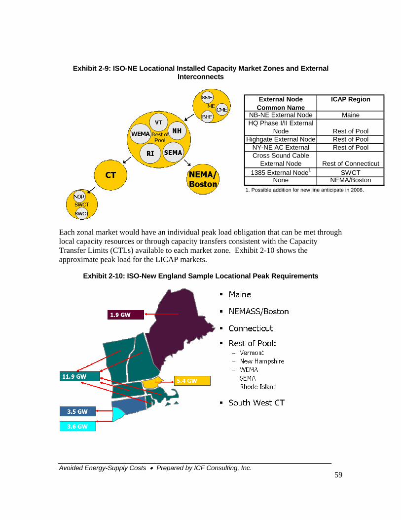
Avoided Energy-Supply Costs • Prepared by ICF Consulting, Inc.
59
Exhibit 2-9: ISO-NE Locational Installed Capacity Market Zones and External Interconnects
Each zonal market would have an individual peak load obligation that can be met through local capacity resources or through capacity transfers consistent with the Capacity Transfer Limits (CTLs) available to each market zone. Exhibit 2-10 shows the approximate peak load for the LICAP markets.
Exhibit 2-10: ISO-New England Sample Locational Peak Requirements
External Node Common Name
ICAP Region
NB-NE External Node MaineHQ Phase I/II External
Node Rest of PoolHighgate External Node Rest of Pool
NY-NE AC External Rest of PoolCross Sound Cable
External Node Rest of Connecticut1385 External Node1 SWCT
None NEMA/Boston1. Possible addition for new line anticipate in 2008.
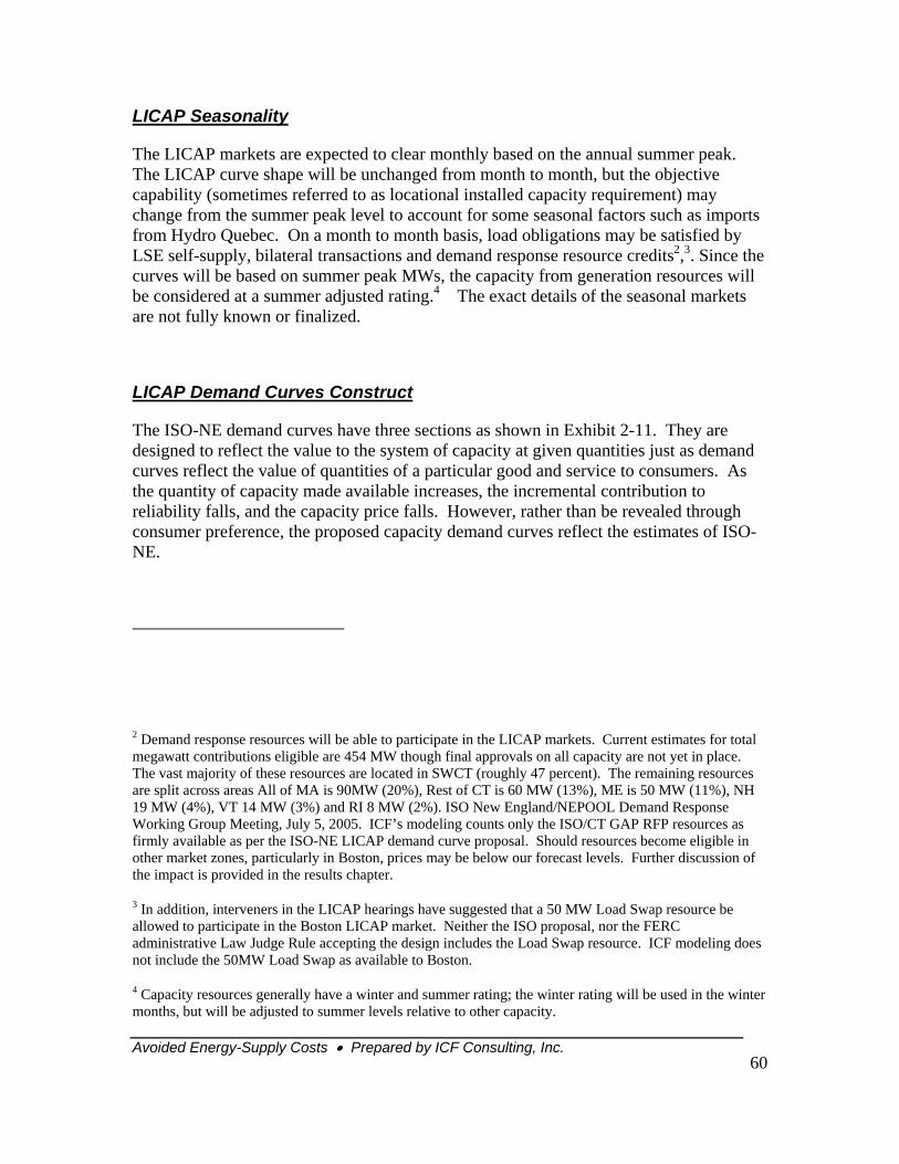
Avoided Energy-Supply Costs • Prepared by ICF Consulting, Inc.
60
LICAP Seasonality
The LICAP markets are expected to clear monthly based on the annual summer peak. The LICAP curve shape will be unchanged from month to month, but the objective capability (sometimes referred to as locational installed capacity requirement) may change from the summer peak level to account for some seasonal factors such as imports from Hydro Quebec. On a month to month basis, load obligations may be satisfied by LSE self-supply, bilateral transactions and demand response resource credits2,3. Since the curves will be based on summer peak MWs, the capacity from generation resources will be considered at a summer adjusted rating.4 The exact details of the seasonal markets are not fully known or finalized.
LICAP Demand Curves Construct
The ISO-NE demand curves have three sections as shown in Exhibit 2-11. They are designed to reflect the value to the system of capacity at given quantities just as demand curves reflect the value of quantities of a particular good and service to consumers. As the quantity of capacity made available increases, the incremental contribution to reliability falls, and the capacity price falls. However, rather than be revealed through consumer preference, the proposed capacity demand curves reflect the estimates of ISO-NE.
2 Demand response resources will be able to participate in the LICAP markets. Current estimates for total megawatt contributions eligible are 454 MW though final approvals on all capacity are not yet in place. The vast majority of these resources are located in SWCT (roughly 47 percent). The remaining resources are split across areas All of MA is 90MW (20%), Rest of CT is 60 MW (13%), ME is 50 MW (11%), NH 19 MW (4%), VT 14 MW (3%) and RI 8 MW (2%). ISO New England/NEPOOL Demand Response Working Group Meeting, July 5, 2005. ICF’s modeling counts only the ISO/CT GAP RFP resources as firmly available as per the ISO-NE LICAP demand curve proposal. Should resources become eligible in other market zones, particularly in Boston, prices may be below our forecast levels. Further discussion of the impact is provided in the results chapter.
3 In addition, interveners in the LICAP hearings have suggested that a 50 MW Load Swap resource be allowed to participate in the Boston LICAP market. Neither the ISO proposal, nor the FERC administrative Law Judge Rule accepting the design includes the Load Swap resource. ICF modeling does not include the 50MW Load Swap as available to Boston.
4 Capacity resources generally have a winter and summer rating; the winter rating will be used in the winter months, but will be adjusted to summer levels relative to other capacity.
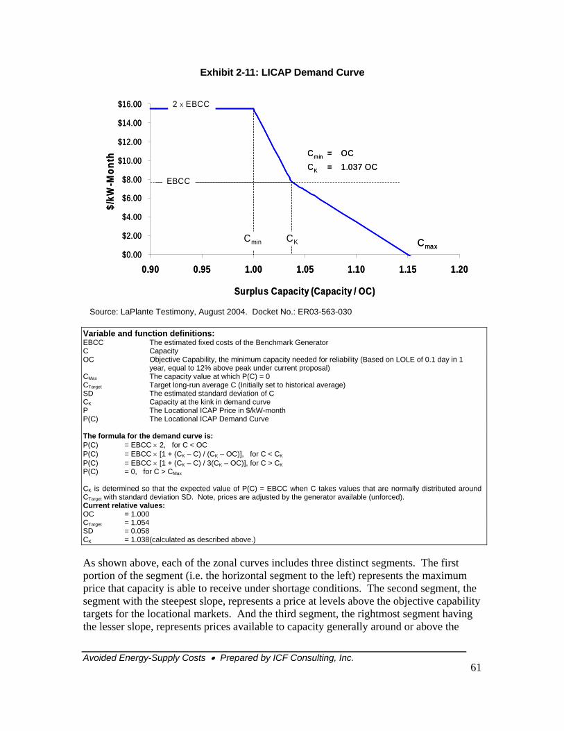
Avoided Energy-Supply Costs • Prepared by ICF Consulting, Inc.
61
Variable and function definitions: EBCC The estimated fixed costs of the Benchmark Generator C Capacity OC Objective Capability, the minimum capacity needed for reliability (Based on LOLE of 0.1 day in 1
year, equal to 12% above peak under current proposal) CMax The capacity value at which P(C) = 0 CTarget Target long-run average C (Initially set to historical average) SD The estimated standard deviation of C CK Capacity at the kink in demand curve P The Locational ICAP Price in $/kW-month P(C) The Locational ICAP Demand Curve The formula for the demand curve is: P(C) = EBCC × 2, for C < OC P(C) = EBCC × [1 + (CK – C) / (CK – OC)], for C < CK
P(C) = EBCC × [1 + (CK – C) / 3(CK – OC)], for C > CKP(C) = 0, for C > CMax CK is determined so that the expected value of P(C) = EBCC when C takes values that are normally distributed around CTarget with standard deviation SD. Note, prices are adjusted by the generator available (unforced). Current relative values: OC = 1.000 CTarget = 1.054 SD = 0.058 CK = 1.038 (calculated as described above.)
As shown above, each of the zonal curves includes three distinct segments. The first portion of the segment (i.e. the horizontal segment to the left) represents the maximum price that capacity is able to receive under shortage conditions. The second segment, the segment with the steepest slope, represents a price at levels above the objective capability targets for the locational markets. And the third segment, the rightmost segment having the lesser slope, represents prices available to capacity generally around or above the
Exhibit 2-11: LICAP Demand Curve
$0.00
$2.00
$4.00
$6.00
$8.00
$10.00
$12.00
$14.00
$16.00
0.90 0.95 1.00 1.05 1.10 1.15 1.20
Surplus Capacity (Capacity / OC)
$/kW
-Mon
th2 X EBCC
EBCC
Cmin CK Cmax
Cmin = OCCK = 1.037 OC
$0.00
$2.00
$4.00
$6.00
$8.00
$10.00
$12.00
$14.00
$16.00
0.90 0.95 1.00 1.05 1.10 1.15 1.20
Surplus Capacity (Capacity / OC)
$/kW
-Mon
th2 X EBCC
EBCC
Cmin CK Cmax
Cmin = OCCK = 1.037 OC
Source: LaPlante Testimony, August 2004. Docket No.: ER03-563-030
Avoided Energy-Supply Costs • Prepared by ICF Consulting, Inc.
62
target reserve capacity in the locational market.
Like any economic demand curve, the capacity demand curves show quantity on the x-axis and price on the y-axis. In this context, the x-axis is further defined as the percent of installed capacity available to the marketplace. The downward slope of the curve indicates that market prices are higher when less installed capacity is available to the marketplace. As more capacity is added to the system, less value is associated with the available capacity and generation providers receive a lower payment for their available capacity.
Several important inputs used to derive the demand curve include the following: the price for new entry (estimated benchmark capacity cost or EBCC); the minimum resources needed for reliable operation (OC or objective capability); the target quantity of capacity resources desired (Ctarget); the maximum quantity of capacity resources that will receive compensation (Cmax); and the quantity of capacity resources that are paid the maximum ceiling price (2xEBCC).
The EBCC reflects the expected fixed and investment costs for new capacity to be installed in local markets. The estimated EBCC value is built from a bottom up approach reflecting the equipment costs, financing costs, and locational cost elements. An example of the component cost assumptions used to determine the EBCC is shown in Exhibit 2-12. The exhibit shows the component costs for SWCT as an illustration of the cost build-up. In order to encourage the entry of new resources, the EBCC price is established to reflect the annual levelized cost of new entry for a simple cycle combustion turbine (CT). Other zones will have comparable calculations; however, each will have its own distinct values based on the installed equipment costs for that location.
Parameters that vary regionally include labor, land and taxes. Boston and SWCT have the highest labor and land costs. Connecticut has the highest property tax rates, but the lowest income tax rates.
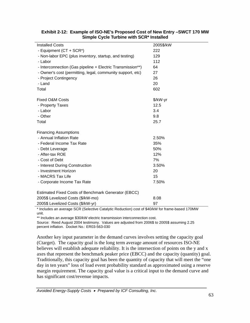
Avoided Energy-Supply Costs • Prepared by ICF Consulting, Inc.
63
Exhibit 2-12: Example of ISO-NE’s Proposed Cost of New Entry –SWCT 170 MW Simple Cycle Turbine with SCR* Installed
Installed Costs 2005$/kW - Equipment (CT + SCR*) 222 - Non-labor EPC (plus inventory, startup, and testing) 129 - Labor 112 - Interconnection (Gas pipeline + Electric Transmission**) 64 - Owner's cost (permitting, legal, community support, etc) 27 - Project Contingency 26 - Land 20 Total 602 Fixed O&M Costs
$/kW-yr
- Property Taxes 12.5 - Labor 3.4 - Other 9.8 Total 25.7 Financing Assumptions
- Annual Inflation Rate 2.50% - Federal Income Tax Rate 35% - Debt Leverage 50% - After-tax ROE 12% - Cost of Debt 7% - Interest During Construction 3.50% - Investment Horizon 20 - MACRS Tax Life 15 - Corporate Income Tax Rate 7.50% Estimated Fixed Costs of Benchmark Generator (EBCC)
2005$ Levelized Costs ($/kW-mo) 8.08 2005$ Levelized Costs ($/kW-yr) 97 * Includes an average SCR (Selective Catalytic Reduction) cost of $40/kW for frame-based 170MW unit. ** Includes an average $30/kW electric transmission interconnection cost. Source: Reed August 2004 testimony. Values are adjusted from 2006$ to 2005$ assuming 2.25 percent inflation. Docket No.: ER03-563-030
Another key input parameter in the demand curves involves setting the capacity goal (Ctarget). The capacity goal is the long term average amount of resources ISO-NE believes will establish adequate reliability. It is the intersection of points on the y and x axes that represent the benchmark peaker price (EBCC) and the capacity (quantity) goal. Traditionally, this capacity goal has been the quantity of capacity that will meet the “one day in ten years” loss of load event probability standard as approximated using a reserve margin requirement. The capacity goal value is a critical input to the demand curve and has significant cost/revenue impacts.
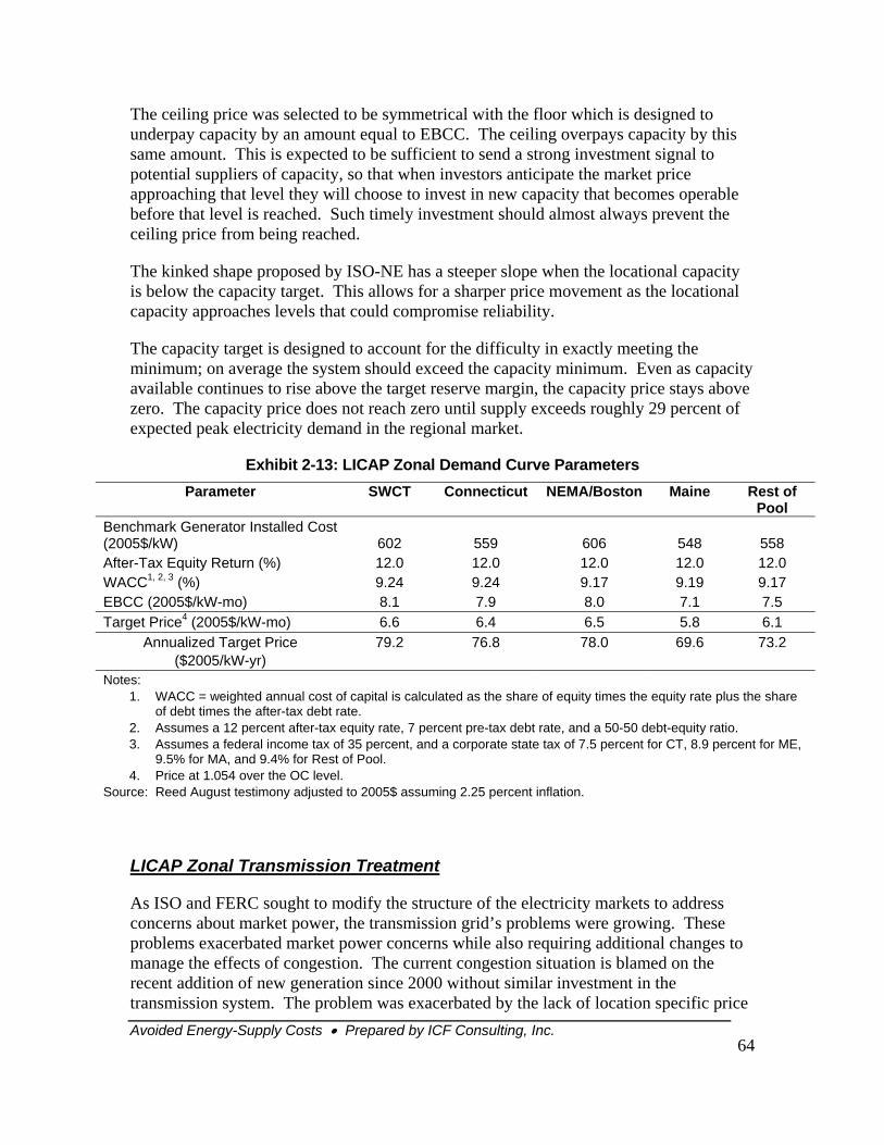
Avoided Energy-Supply Costs • Prepared by ICF Consulting, Inc.
64
The ceiling price was selected to be symmetrical with the floor which is designed to underpay capacity by an amount equal to EBCC. The ceiling overpays capacity by this same amount. This is expected to be sufficient to send a strong investment signal to potential suppliers of capacity, so that when investors anticipate the market price approaching that level they will choose to invest in new capacity that becomes operable before that level is reached. Such timely investment should almost always prevent the ceiling price from being reached.
The kinked shape proposed by ISO-NE has a steeper slope when the locational capacity is below the capacity target. This allows for a sharper price movement as the locational capacity approaches levels that could compromise reliability.
The capacity target is designed to account for the difficulty in exactly meeting the minimum; on average the system should exceed the capacity minimum. Even as capacity available continues to rise above the target reserve margin, the capacity price stays above zero. The capacity price does not reach zero until supply exceeds roughly 29 percent of expected peak electricity demand in the regional market.
Exhibit 2-13: LICAP Zonal Demand Curve Parameters Parameter SWCT Connecticut NEMA/Boston Maine Rest of
Pool Benchmark Generator Installed Cost (2005$/kW) 602 559 606 548 558 After-Tax Equity Return (%) 12.0 12.0 12.0 12.0 12.0 WACC1, 2, 3 (%) 9.24 9.24 9.17 9.19 9.17 EBCC (2005$/kW-mo) 8.1 7.9 8.0 7.1 7.5 Target Price4 (2005$/kW-mo) 6.6 6.4 6.5 5.8 6.1
Annualized Target Price ($2005/kW-yr)
79.2 76.8 78.0 69.6 73.2
Notes: 1. WACC = weighted annual cost of capital is calculated as the share of equity times the equity rate plus the share
of debt times the after-tax debt rate. 2. Assumes a 12 percent after-tax equity rate, 7 percent pre-tax debt rate, and a 50-50 debt-equity ratio. 3. Assumes a federal income tax of 35 percent, and a corporate state tax of 7.5 percent for CT, 8.9 percent for ME,
9.5% for MA, and 9.4% for Rest of Pool. 4. Price at 1.054 over the OC level.
Source: Reed August testimony adjusted to 2005$ assuming 2.25 percent inflation.
LICAP Zonal Transmission Treatment
As ISO and FERC sought to modify the structure of the electricity markets to address concerns about market power, the transmission grid’s problems were growing. These problems exacerbated market power concerns while also requiring additional changes to manage the effects of congestion. The current congestion situation is blamed on the recent addition of new generation since 2000 without similar investment in the transmission system. The problem was exacerbated by the lack of location specific price
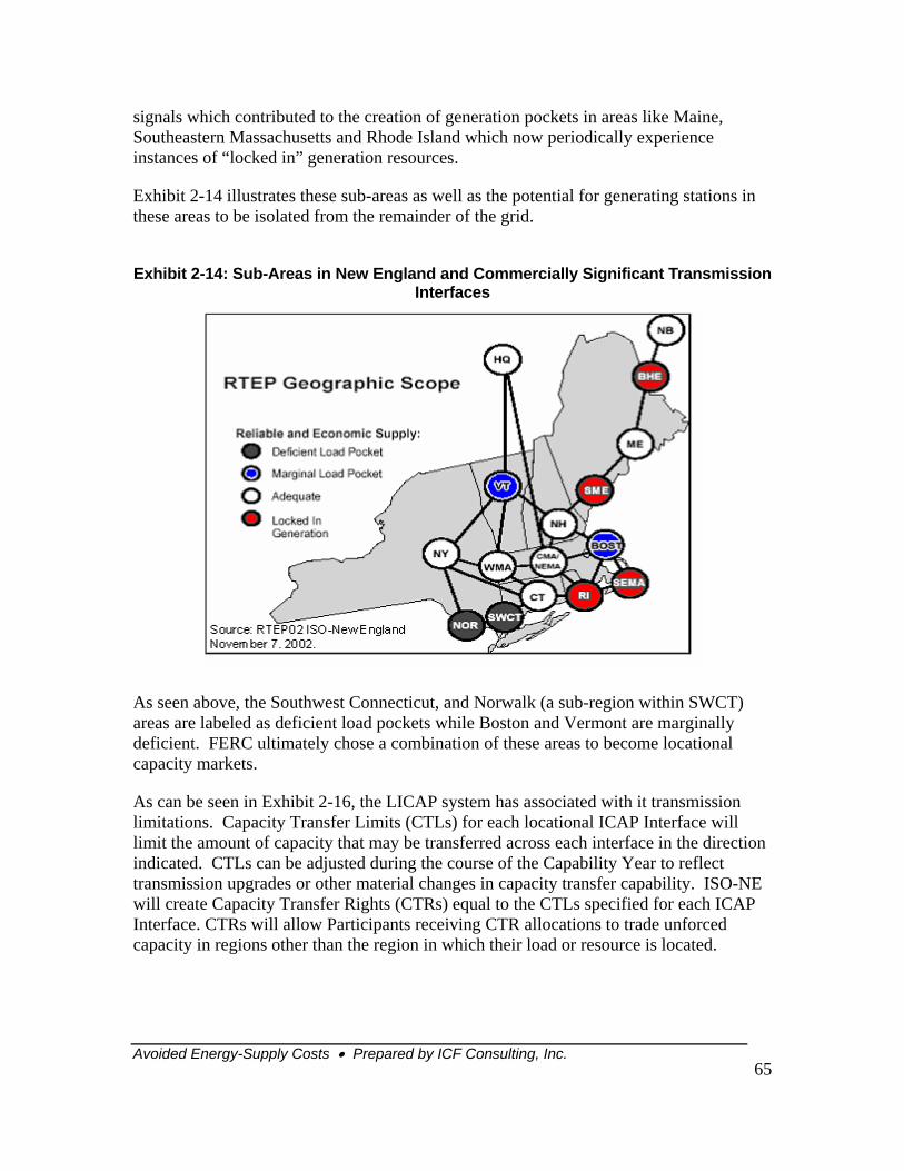
Avoided Energy-Supply Costs • Prepared by ICF Consulting, Inc.
65
signals which contributed to the creation of generation pockets in areas like Maine, Southeastern Massachusetts and Rhode Island which now periodically experience instances of “locked in” generation resources.
Exhibit 2-14 illustrates these sub-areas as well as the potential for generating stations in these areas to be isolated from the remainder of the grid.
Exhibit 2-14: Sub-Areas in New England and Commercially Significant Transmission
Interfaces
As seen above, the Southwest Connecticut, and Norwalk (a sub-region within SWCT) areas are labeled as deficient load pockets while Boston and Vermont are marginally deficient. FERC ultimately chose a combination of these areas to become locational capacity markets.
As can be seen in Exhibit 2-16, the LICAP system has associated with it transmission limitations. Capacity Transfer Limits (CTLs) for each locational ICAP Interface will limit the amount of capacity that may be transferred across each interface in the direction indicated. CTLs can be adjusted during the course of the Capability Year to reflect transmission upgrades or other material changes in capacity transfer capability. ISO-NE will create Capacity Transfer Rights (CTRs) equal to the CTLs specified for each ICAP Interface. CTRs will allow Participants receiving CTR allocations to trade unforced capacity in regions other than the region in which their load or resource is located.
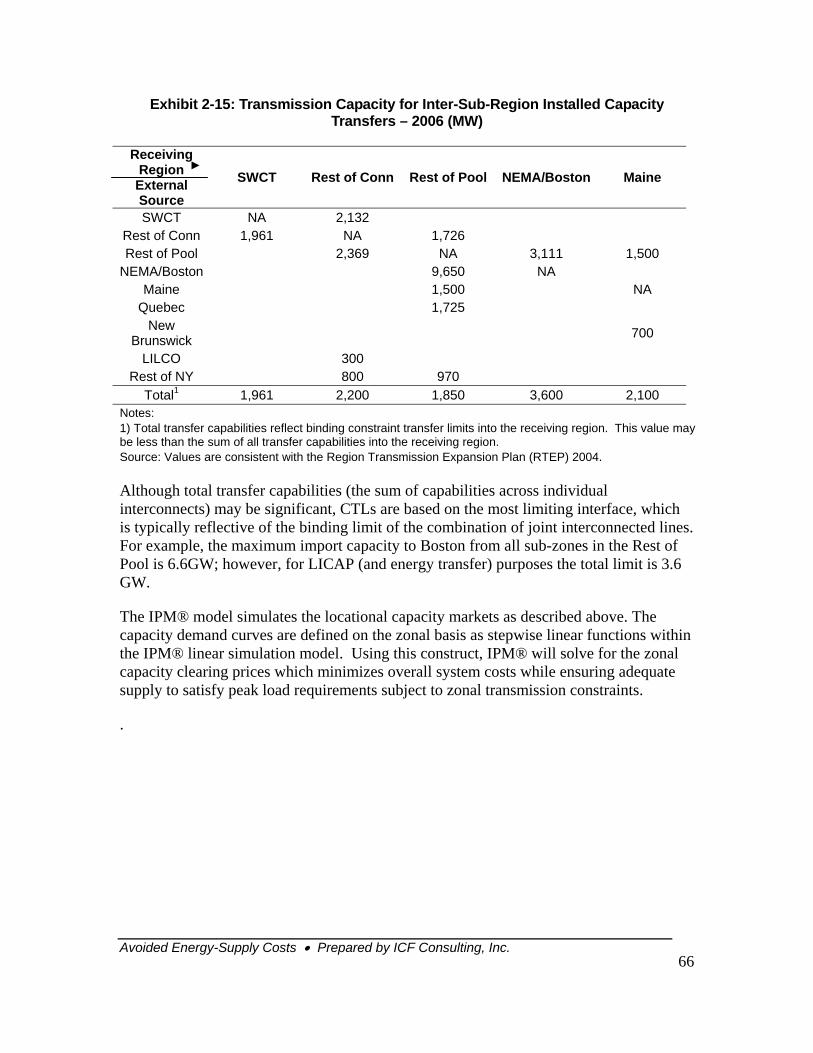
Avoided Energy-Supply Costs • Prepared by ICF Consulting, Inc.
66
Exhibit 2-15: Transmission Capacity for Inter-Sub-Region Installed Capacity Transfers – 2006 (MW)
Although total transfer capabilities (the sum of capabilities across individual interconnects) may be significant, CTLs are based on the most limiting interface, which is typically reflective of the binding limit of the combination of joint interconnected lines. For example, the maximum import capacity to Boston from all sub-zones in the Rest of Pool is 6.6GW; however, for LICAP (and energy transfer) purposes the total limit is 3.6 GW.
The IPM® model simulates the locational capacity markets as described above. The capacity demand curves are defined on the zonal basis as stepwise linear functions within the IPM® linear simulation model. Using this construct, IPM® will solve for the zonal capacity clearing prices which minimizes overall system costs while ensuring adequate supply to satisfy peak load requirements subject to zonal transmission constraints.
.
Receiving Region External Source
SWCT Rest of Conn Rest of Pool NEMA/Boston Maine
SWCT NA 2,132 Rest of Conn 1,961 NA 1,726 Rest of Pool 2,369 NA 3,111 1,500
NEMA/Boston 9,650 NA Maine 1,500 NA
Quebec 1,725 New
Brunswick 700
LILCO 300 Rest of NY 800 970
Total1 1,961 2,200 1,850 3,600 2,100 Notes: 1) Total transfer capabilities reflect binding constraint transfer limits into the receiving region. This value may be less than the sum of all transfer capabilities into the receiving region. Source: Values are consistent with the Region Transmission Expansion Plan (RTEP) 2004.
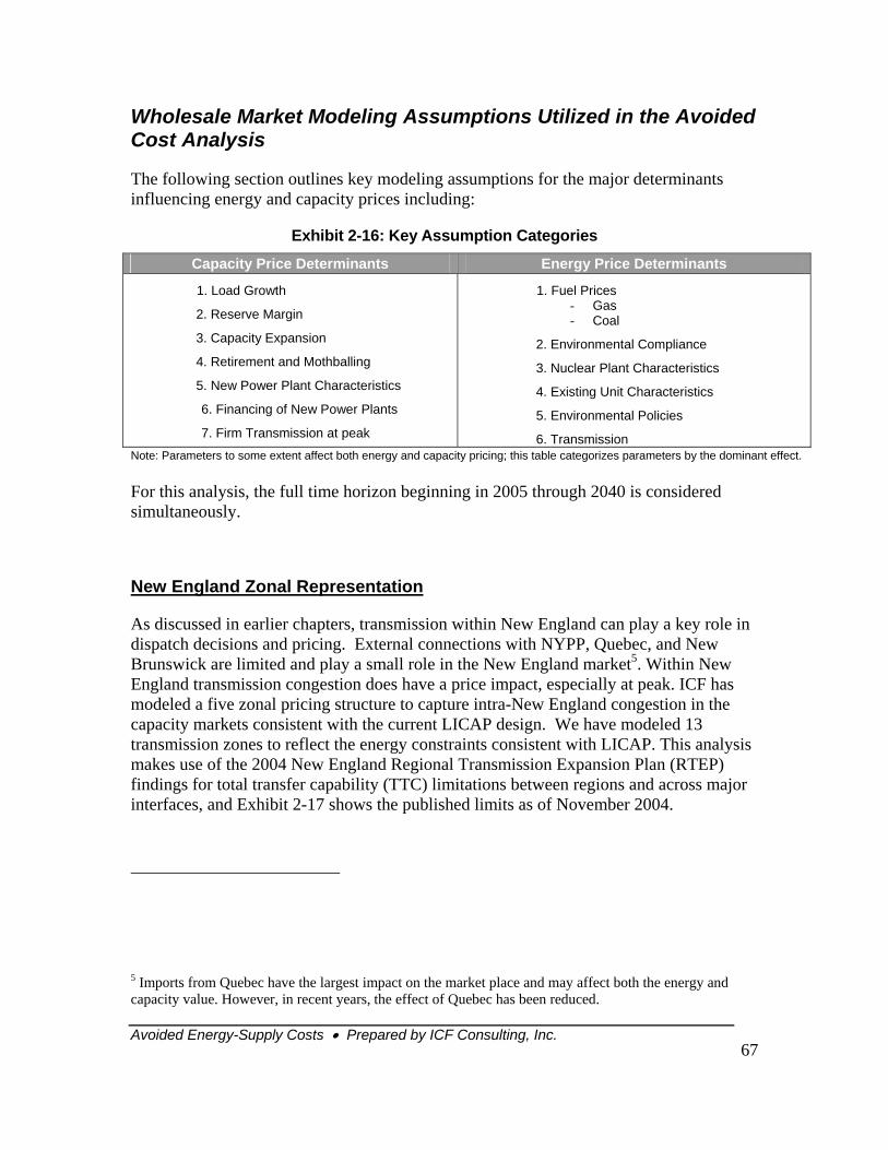
Avoided Energy-Supply Costs • Prepared by ICF Consulting, Inc.
67
Wholesale Market Modeling Assumptions Utilized in the Avoided Cost Analysis
The following section outlines key modeling assumptions for the major determinants influencing energy and capacity prices including:
Exhibit 2-16: Key Assumption Categories
Capacity Price Determinants Energy Price Determinants
1. Load Growth
2. Reserve Margin
3. Capacity Expansion
4. Retirement and Mothballing
5. New Power Plant Characteristics
6. Financing of New Power Plants
7. Firm Transmission at peak
1. Fuel Prices - Gas - Coal
2. Environmental Compliance
3. Nuclear Plant Characteristics
4. Existing Unit Characteristics
5. Environmental Policies
6. Transmission Note: Parameters to some extent affect both energy and capacity pricing; this table categorizes parameters by the dominant effect.
For this analysis, the full time horizon beginning in 2005 through 2040 is considered simultaneously.
New England Zonal Representation
As discussed in earlier chapters, transmission within New England can play a key role in dispatch decisions and pricing. External connections with NYPP, Quebec, and New Brunswick are limited and play a small role in the New England market5. Within New England transmission congestion does have a price impact, especially at peak. ICF has modeled a five zonal pricing structure to capture intra-New England congestion in the capacity markets consistent with the current LICAP design. We have modeled 13 transmission zones to reflect the energy constraints consistent with LICAP. This analysis makes use of the 2004 New England Regional Transmission Expansion Plan (RTEP) findings for total transfer capability (TTC) limitations between regions and across major interfaces, and Exhibit 2-17 shows the published limits as of November 2004.
5 Imports from Quebec have the largest impact on the market place and may affect both the energy and capacity value. However, in recent years, the effect of Quebec has been reduced.
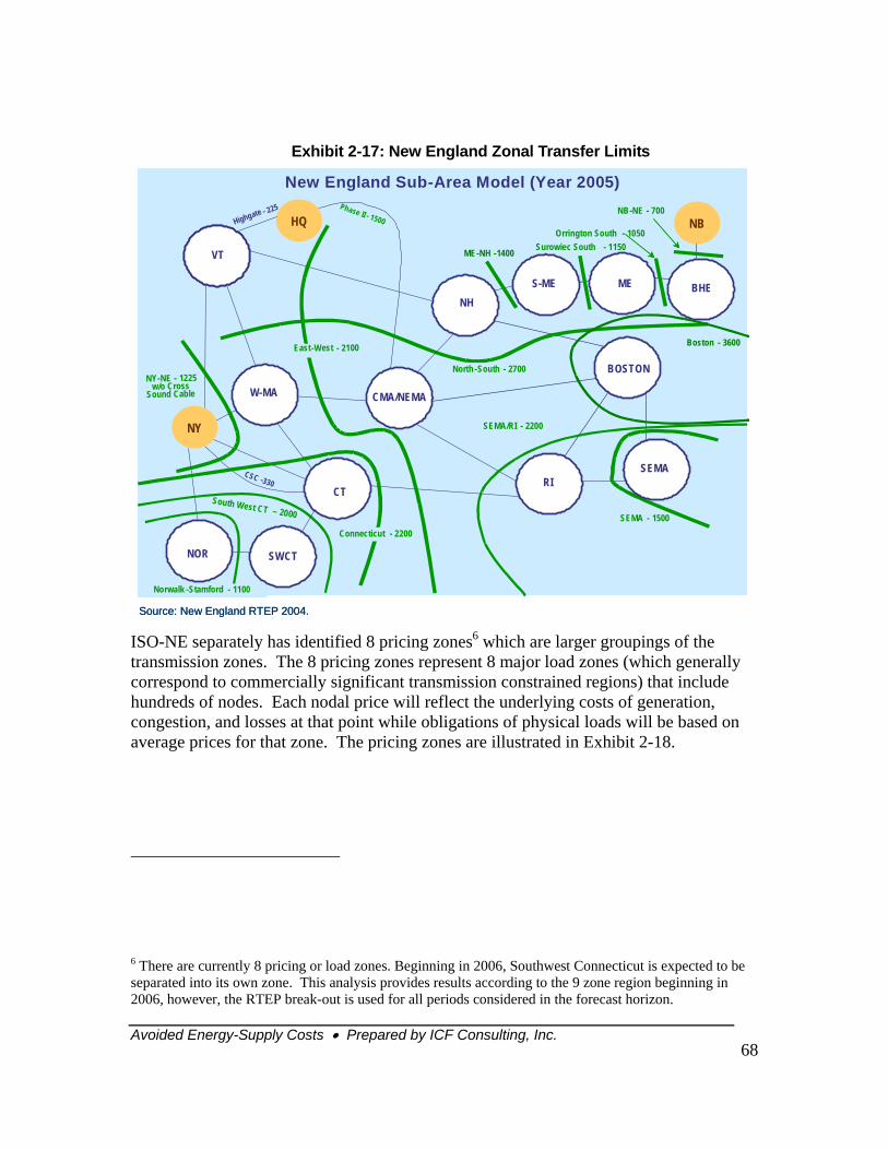
Avoided Energy-Supply Costs • Prepared by ICF Consulting, Inc. 68
Exhibit 2-17: New England Zonal Transfer Limits
ISO-NE separately has identified 8 pricing zones6 which are larger groupings of the transmission zones. The 8 pricing zones represent 8 major load zones (which generally correspond to commercially significant transmission constrained regions) that include hundreds of nodes. Each nodal price will reflect the underlying costs of generation, congestion, and losses at that point while obligations of physical loads will be based on average prices for that zone. The pricing zones are illustrated in Exhibit 2-18.
6 There are currently 8 pricing or load zones. Beginning in 2006, Southwest Connecticut is expected to be separated into its own zone. This analysis provides results according to the 9 zone region beginning in 2006, however, the RTEP break-out is used for all periods considered in the forecast horizon.
SEMA - 1500
NY-NE - 1225w/o Cross
Sound Cable
Norwalk -Stamford - 1100
Surowiec South - 1150ME-NH -1400
North -South - 2700
Boston - 3600
NBOrrington South - 1050
NB-NE - 700HQHighgate - 225
- 0
CSC -330
Phase II 150
S-ME ME BHE
SEMARI
W-MA CMA/NEMA
New England Sub-Area Model (Year 2005)
NY
NH
BOSTON
CT
SWCTNOR
Connecticut - 2200
South West CT – 2000
East-West - 2100
VT
SWCT
SEMA/RI - 2200
Source: New England RTEP 2004.
SEMA - 1500
NY-NE - 1225w/o Cross
Sound Cable
Norwalk -Stamford - 1100
Surowiec South - 1150ME-NH -1400
North -South - 2700
Boston - 3600
NBOrrington South - 1050
NB-NE - 700HQHighgate - 225
- 0
CSC -330
Phase II 150
S-ME ME BHE
SEMARI
W-MA CMA/NEMA
New England Sub-Area Model (Year 2005)
NY
NH
BOSTON
CT
SWCTNOR
Connecticut - 2200
South West CT – 2000
East-West - 2100
VT
SWCT
SEMA/RI - 2200
SEMA - 1500
NY-NE - 1225w/o Cross
Sound Cable
Norwalk -Stamford - 1100
Surowiec South - 1150ME-NH -1400
North -South - 2700
Boston - 3600
NBOrrington South - 1050
NB-NE - 700HQHighgate - 225
- 0
CSC -330
Phase II 150
S-ME ME BHE
SEMARI
W-MA CMA/NEMA
New England Sub-Area Model (Year 2005)
NY
NH
BOSTON
CT
SWCTNOR
Connecticut - 2200
South West CT – 2000
East-West - 2100
VT
SWCT
Source: New England RTEP 2004.
SEMA/RI - 2200
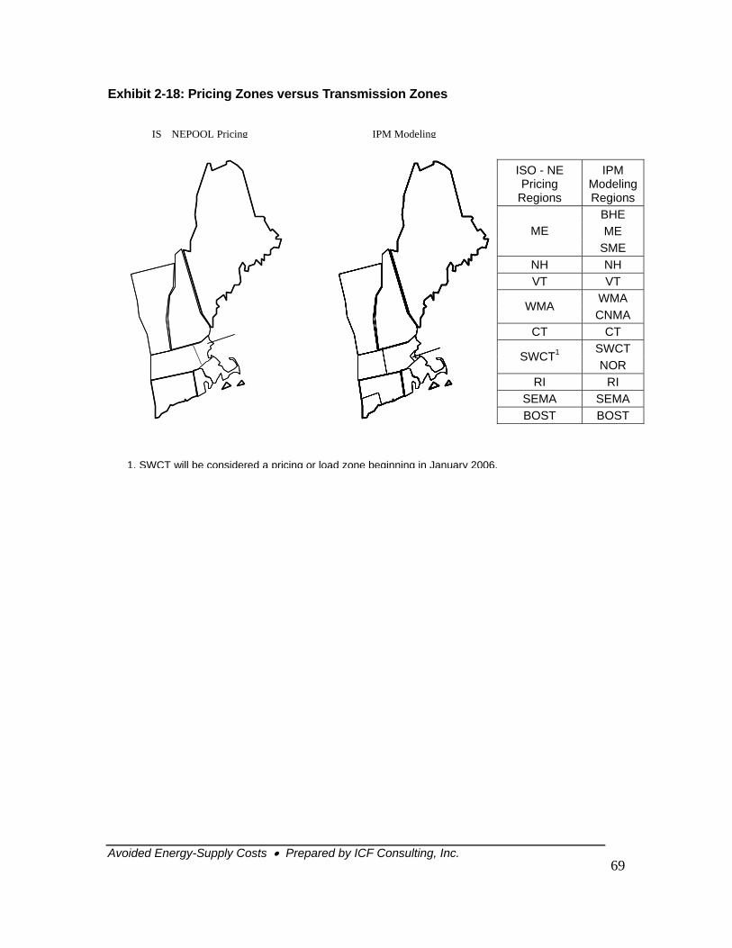
Av
Exhibit 2-18: Pricing Zones versus Transmission Zones
ISO - NE Pricing
Regions
IPM Modeling Regions
BHE ME ME
SME NH NH VT VT
WMA WMA
CNMA CT CT
SWCT SWCT1
NOR RI RI
SEMA SEMA BOST BOST
IS NEPOOL Pricing IPM Modeling
1. SWCT will be considered a pricing or load zone beginning in January 2006.
oided Energy-Supply Costs • Prepared by ICF Consulting, Inc. 69
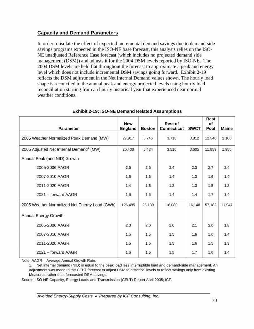
Avoided Energy-Supply Costs • Prepared by ICF Consulting, Inc.
70
Capacity and Demand Parameters
In order to isolate the effect of expected incremental demand savings due to demand side savings programs expected in the ISO-NE base forecast, this analysis relies on the ISO-NE unadjusted Reference Case forecast (which includes no projected demand side management (DSM)) and adjusts it for the 2004 DSM levels reported by ISO-NE. The 2004 DSM levels are held flat throughout the forecast to approximate a peak and energy level which does not include incremental DSM savings going forward. Exhibit 2-19 reflects the DSM adjustment in the Net Internal Demand values shown. The hourly load shape is reconciled to the annual peak and energy projected levels using hourly load reconciliation starting from an hourly historical year that experienced near normal weather conditions.
Exhibit 2-19: ISO-NE Demand Related Assumptions
Parameter New
England BostonRest of
Connecticut SWCT
Rest of
Pool Maine
2005 Weather Normalized Peak Demand (MW) 27,917 5,746 3,718 3,812 12,540 2,100
2005 Adjusted Net Internal Demand1 (MW) 26,400 5,434 3,516 3,605 11,859 1,986
Annual Peak (and NID) Growth
2005-2006 AAGR 2.5 2.6 2.4 2.3 2.7 2.4
2007-2010 AAGR 1.5 1.5 1.4 1.3 1.6 1.4
2011-2020 AAGR 1.4 1.5 1.3 1.3 1.5 1.3
2021 – forward AAGR 1.6 1.6 1.4 1.4 1.7 1.4
2005 Weather Normalized Net Energy Load (GWh) 126,495 25,139 16,080 16,148 57,182 11,947
Annual Energy Growth
2005-2006 AAGR 2.0 2.0 2.0 2.1 2.0 1.8
2007-2010 AAGR 1.5 1.5 1.5 1.6 1.6 1.4
2011-2020 AAGR 1.5 1.5 1.5 1.6 1.5 1.3
2021 – forward AAGR 1.6 1.5 1.5 1.7 1.6 1.4
Note: AAGR = Average Annual Growth Rate. 1. Net internal demand (NID) is equal to the peak load less interruptible load and demand-side management. An adjustment was made to the CELT forecast to adjust DSM to historical levels to reflect savings only from existing Measures rather than forecasted DSM savings.
Source: ISO-NE Capacity, Energy Loads and Transmission (CELT) Report April 2005; ICF.
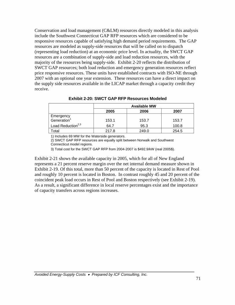
Avoided Energy-Supply Costs • Prepared by ICF Consulting, Inc.
71
Conservation and load management (C&LM) resources directly modeled in this analysis include the Southwest Connecticut GAP RFP resources which are considered to be responsive resources capable of satisfying high demand period requirements. The GAP resources are modeled as supply-side resources that will be called on to dispatch (representing load reduction) at an economic price level. In actuality, the SWCT GAP resources are a combination of supply-side and load reduction resources, with the majority of the resources being supply-side. Exhibit 2-20 reflects the distribution of SWCT GAP resources; both load reduction and emergency generation resources reflect price responsive resources. These units have established contracts with ISO-NE through 2007 with an optional one year extension. These resources can have a direct impact on the supply side resources available in the LICAP market through a capacity credit they receive.
Exhibit 2-20: SWCT GAP RFP Resources Modeled
Available MW 2005 2006 2007
Emergency Generation1 153.1 153.7 153.7 Load Reduction2,3 64.7 95.3 100.8 Total 217.8 249.0 254.5 1) Includes 69 MW for the Waterside generators. 2) SWCT GAP RFP resources are equally split between Norwalk and Southwest Connecticut model regions. 3) Total cost for the SWCT GAP RFP from 2004-2007 is $492.9/kW (real 2005$).
Exhibit 2-21 shows the available capacity in 2005, which for all of New England represents a 21 percent reserve margin over the net internal demand measure shown in Exhibit 2-19. Of this total, more than 50 percent of the capacity is located in Rest of Pool and roughly 10 percent is located in Boston. In contrast roughly 45 and 20 percent of the coincident peak load occurs in Rest of Pool and Boston respectively (see Exhibit 2-19). As a result, a significant difference in local reserve percentages exist and the importance of capacity transfers across regions increases.
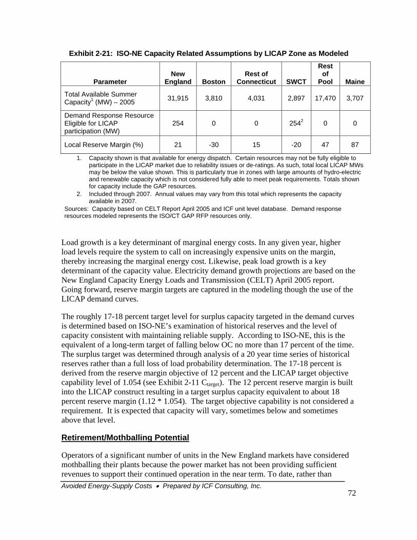
Avoided Energy-Supply Costs • Prepared by ICF Consulting, Inc.
72
Exhibit 2-21: ISO-NE Capacity Related Assumptions by LICAP Zone as Modeled
Parameter New
England Boston Rest of
Connecticut SWCT
Rest of
Pool Maine
Total Available Summer Capacity1 (MW) – 2005 31,915 3,810 4,031 2,897 17,470 3,707
Demand Response Resource Eligible for LICAP participation (MW)
254 0 0 2542 0 0
Local Reserve Margin (%) 21 -30 15 -20 47 87
1. Capacity shown is that available for energy dispatch. Certain resources may not be fully eligible to participate in the LICAP market due to reliability issues or de-ratings. As such, total local LICAP MWs may be below the value shown. This is particularly true in zones with large amounts of hydro-electric and renewable capacity which is not considered fully able to meet peak requirements. Totals shown for capacity include the GAP resources.
2. Included through 2007. Annual values may vary from this total which represents the capacity available in 2007.
Sources: Capacity based on CELT Report April 2005 and ICF unit level database. Demand response resources modeled represents the ISO/CT GAP RFP resources only.
Load growth is a key determinant of marginal energy costs. In any given year, higher load levels require the system to call on increasingly expensive units on the margin, thereby increasing the marginal energy cost. Likewise, peak load growth is a key determinant of the capacity value. Electricity demand growth projections are based on the New England Capacity Energy Loads and Transmission (CELT) April 2005 report. Going forward, reserve margin targets are captured in the modeling though the use of the LICAP demand curves.
The roughly 17-18 percent target level for surplus capacity targeted in the demand curves is determined based on ISO-NE’s examination of historical reserves and the level of capacity consistent with maintaining reliable supply. According to ISO-NE, this is the equivalent of a long-term target of falling below OC no more than 17 percent of the time. The surplus target was determined through analysis of a 20 year time series of historical reserves rather than a full loss of load probability determination. The 17-18 percent is derived from the reserve margin objective of 12 percent and the LICAP target objective capability level of 1.054 (see Exhibit 2-11 Ctarget). The 12 percent reserve margin is built into the LICAP construct resulting in a target surplus capacity equivalent to about 18 percent reserve margin (1.12 * 1.054). The target objective capability is not considered a requirement. It is expected that capacity will vary, sometimes below and sometimes above that level.
Retirement/Mothballing Potential
Operators of a significant number of units in the New England markets have considered mothballing their plants because the power market has not been providing sufficient revenues to support their continued operation in the near term. To date, rather than
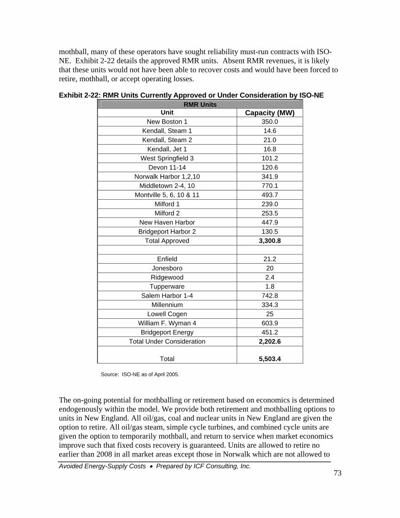
Avoided Energy-Supply Costs • Prepared by ICF Consulting, Inc.
73
mothball, many of these operators have sought reliability must-run contracts with ISO-NE. Exhibit 2-22 details the approved RMR units. Absent RMR revenues, it is likely that these units would not have been able to recover costs and would have been forced to retire, mothball, or accept operating losses.
Exhibit 2-22: RMR Units Currently Approved or Under Consideration by ISO-NE RMR Units
Unit Capacity (MW) New Boston 1 350.0
Kendall, Steam 1 14.6 Kendall, Steam 2 21.0
Kendall, Jet 1 16.8 West Springfield 3 101.2
Devon 11-14 120.6 Norwalk Harbor 1,2,10 341.9
Middletown 2-4, 10 770.1 Montville 5, 6, 10 & 11 493.7
Milford 1 239.0 Milford 2 253.5
New Haven Harbor 447.9 Bridgeport Harbor 2 130.5
Total Approved 3,300.8
Enfield 21.2 Jonesboro 20 Ridgewood 2.4 Tupperware 1.8
Salem Harbor 1-4 742.8 Millennium 334.3
Lowell Cogen 25 William F. Wyman 4 603.9 Bridgeport Energy 451.2
Total Under Consideration 2,202.6
Total 5,503.4
Source: ISO-NE as of April 2005.
The on-going potential for mothballing or retirement based on economics is determined endogenously within the model. We provide both retirement and mothballing options to units in New England. All oil/gas, coal and nuclear units in New England are given the option to retire. All oil/gas steam, simple cycle turbines, and combined cycle units are given the option to temporarily mothball, and return to service when market economics improve such that fixed costs recovery is guaranteed. Units are allowed to retire no earlier than 2008 in all market areas except those in Norwalk which are not allowed to
Avoided Energy-Supply Costs • Prepared by ICF Consulting, Inc.
74
retire until 2010.
The retirement and mothball options are chosen within the model based on projected discounted cash flows. That is, if a unit cannot recover projected fixed costs on a net present value basis over its remaining life, that unit will decide to exit the market and avoid forward losses. The physical costs to mothball, ongoing costs to maintain a mothballed state, and actual costs to return to service are all considered within this construct. The mothballing option is made on a shorter-term basis taking annual revenues and costs into consideration as well as the costs of a mothball unit returning to service. This analysis assumes that units are not allowed to retire from the grid until 2008 at the earliest throughout New England. These assumptions to delay possible retirements to at the earliest 2008 and 2010 were agreed upon by the AESC Study Group to reflect a fairly significant lead time for approval of retirements in general, and a severe need for local capacity in Norwalk.
In this analysis, units currently qualified as RMR are also given economic mothball and retirement options in this analysis, though if required for reliability they will not be allowed to mothball or retire until the reliability constraints are relieved. However, units required for reliability reasons are allowed to recover costs on a cost of service basis through out-of-market mechanisms (such as the existing RMR contracts) even after the LICAP market has begun.
The RMR assumptions are designed to reflect restrictions that are not entirely true to perfectly competitive markets. Since the RMR capacity is available to the market and the capacity contributes into the LICAP clearing level, the resulting LICAP price would be lower than had these units been allowed to mothball or retire based on their economics only. Since the units are forced to stay on (in most cases despite their own declaration of desire to mothball or retire), often to compensate for voltage stability issues, they are compensated through a separate payment which allows the units to receive cost recovery at rate of return deemed to be reasonable by FERC. The effect of allowing these units to retire in the modeling analysis performed would be to drive capacity prices up in those areas with RMR units. This pure economic effect was not considered due to issues such as voltage stability which were not directly modeled in the analysis. That is, in the real world, severe voltage stability issues could result if the units that when modeled would want to retire were allowed to actually exit the market. ISO-New England has historically allowed these units to capture costs and the LICAP design does permit this same RMR activity to continue into the future. As such, assumptions to prevent exit until the stability and reliability issues are addressed are reasonable.
Firmly Planned Supply Additions
Firm supply additions, that is generation builds either recently operational or currently under construction, are explicitly included in the model. Non-firm supply additions are constructed internally by the model to ensure that reserve requirements are achieved through the addition of the most economical power plant technology option available.
Avoided Energy-Supply Costs • Prepared by ICF Consulting, Inc.
75
Additional announced capacity is not included in our model; however, optimal unplanned capacity expansion is determined within the model based on economics. The assumptions used for costs and potential timing of new (unplanned) units are described in the next section.
New Unit Characteristics
In order meet net internal peak demand, the IPM® model will optimize the generation mix to include required new capacity. Characteristics assumed for new unit options drive decisions on the mix of new builds and consequently affect prices. Combustion turbines have the lowest capital and fixed O&M costs among all of the new equipment options. However, this advantage is offset by its higher variable operating costs associated with higher heat rates and higher variable O&M costs. The decisions on what type of capacity, the amount of capacity, and the location of capacity are all internal to the modeling analysis. The modeling tool uses a linear optimization approach with the goal of minimizing costs over the entire time horizon subject to constraints such as ensuring adequate capacity to serve peak and hourly load. We assume costs for new units consistent with those in the ISO-NE demand curve construct.
ICF has explicitly included unplanned build options for the following capacity types in New England:
• Simple Cycle Combustion Turbines (consistent with costs in ISO proposal)
• Combined Cycles (derived from simple cycle costs)
• Cogeneration units (limited amounts of capacity are assumed available based on available sites)
• Renewables (Wind, Biomass, Landfill Gas)
ICF does not consider coal units as an option in New England due to high costs, environmental barriers, and siting limitations.
New simple cycle units are assumed to be available at a levelized cost that ranges from $547/kW to $620/kW (costs vary by region) in New England. New combined cycle and cogeneration costs are assumed to be available at a levelized cost that ranges from $792/kW to $914/kW (2005$). New England costs on an equivalent megawatt basis are slightly higher than the US average when considered on an International Standards Organization (ISO) basis (69°F and sea-level) due to ambient conditions and labor costs. New England summer and site-specific altitude conditions result in a roughly a 4 percent derate for turbine-based capacity output relative to ISO conditions. The average summer temperature is 82 degrees Fahrenheit and the average altitude is 100 feet.
ICF incorporates both the existing cogeneration capacity available to the grid and the
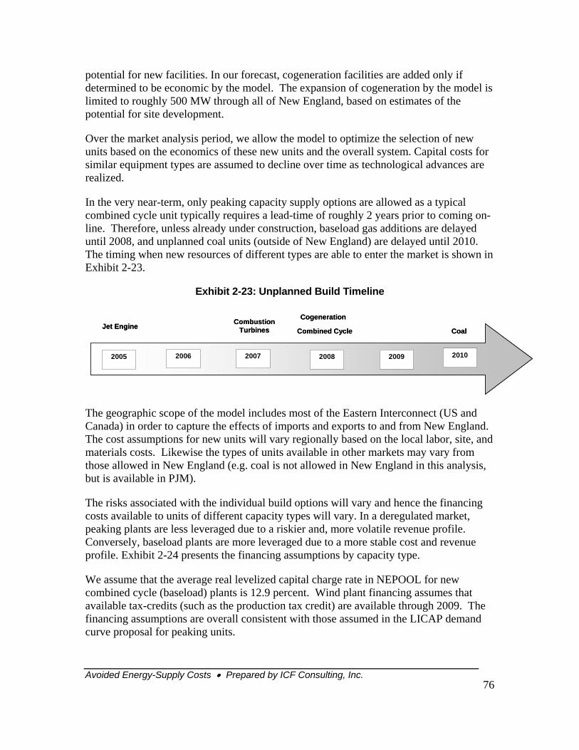
Avoided Energy-Supply Costs • Prepared by ICF Consulting, Inc.
76
potential for new facilities. In our forecast, cogeneration facilities are added only if determined to be economic by the model. The expansion of cogeneration by the model is limited to roughly 500 MW through all of New England, based on estimates of the potential for site development.
Over the market analysis period, we allow the model to optimize the selection of new units based on the economics of these new units and the overall system. Capital costs for similar equipment types are assumed to decline over time as technological advances are realized.
In the very near-term, only peaking capacity supply options are allowed as a typical combined cycle unit typically requires a lead-time of roughly 2 years prior to coming on-line. Therefore, unless already under construction, baseload gas additions are delayed until 2008, and unplanned coal units (outside of New England) are delayed until 2010. The timing when new resources of different types are able to enter the market is shown in Exhibit 2-23.
Exhibit 2-23: Unplanned Build Timeline
The geographic scope of the model includes most of the Eastern Interconnect (US and Canada) in order to capture the effects of imports and exports to and from New England. The cost assumptions for new units will vary regionally based on the local labor, site, and materials costs. Likewise the types of units available in other markets may vary from those allowed in New England (e.g. coal is not allowed in New England in this analysis, but is available in PJM).
The risks associated with the individual build options will vary and hence the financing costs available to units of different capacity types will vary. In a deregulated market, peaking plants are less leveraged due to a riskier and, more volatile revenue profile. Conversely, baseload plants are more leveraged due to a more stable cost and revenue profile. Exhibit 2-24 presents the financing assumptions by capacity type.
We assume that the average real levelized capital charge rate in NEPOOL for new combined cycle (baseload) plants is 12.9 percent. Wind plant financing assumes that available tax-credits (such as the production tax credit) are available through 2009. The financing assumptions are overall consistent with those assumed in the LICAP demand curve proposal for peaking units.
Combustion TurbinesJet Engine Combined Cycle
Cogeneration
Coal
2005 2006 20082007 2009 2010
Combustion TurbinesJet Engine Combined Cycle
Cogeneration
Coal
2005 2006 20082007 2009 2010
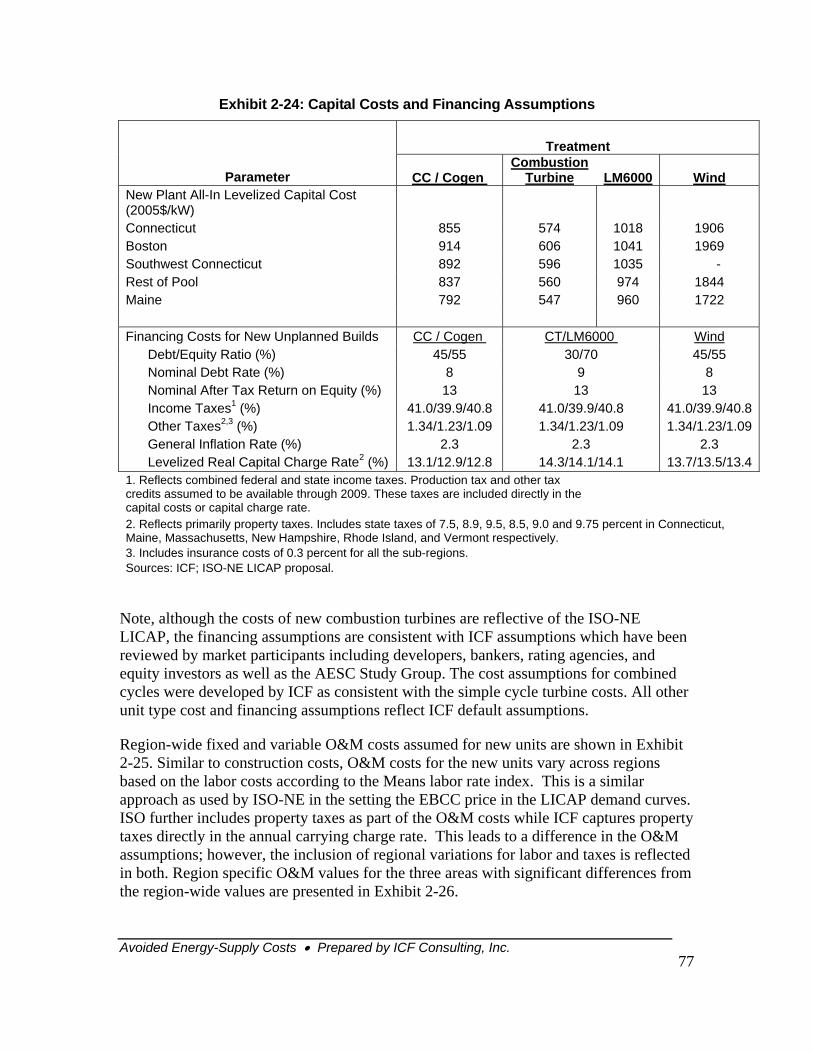
Avoided Energy-Supply Costs • Prepared by ICF Consulting, Inc.
77
Exhibit 2-24: Capital Costs and Financing Assumptions
Treatment
Parameter CC / Cogen Combustion
Turbine LM6000 WindNew Plant All-In Levelized Capital Cost (2005$/kW) Connecticut 855 574 1018 1906 Boston 914 606 1041 1969 Southwest Connecticut 892 596 1035 - Rest of Pool 837 560 974 1844 Maine 792 547 960 1722 Financing Costs for New Unplanned Builds CC / Cogen CT/LM6000 Wind Debt/Equity Ratio (%) 45/55 30/70 45/55 Nominal Debt Rate (%) 8 9 8 Nominal After Tax Return on Equity (%) 13 13 13 Income Taxes1 (%) 41.0/39.9/40.8 41.0/39.9/40.8 41.0/39.9/40.8 Other Taxes2,3 (%) 1.34/1.23/1.09 1.34/1.23/1.09 1.34/1.23/1.09 General Inflation Rate (%) 2.3 2.3 2.3 Levelized Real Capital Charge Rate2 (%) 13.1/12.9/12.8 14.3/14.1/14.1 13.7/13.5/13.41. Reflects combined federal and state income taxes. Production tax and other tax credits assumed to be available through 2009. These taxes are included directly in the capital costs or capital charge rate.
2. Reflects primarily property taxes. Includes state taxes of 7.5, 8.9, 9.5, 8.5, 9.0 and 9.75 percent in Connecticut, Maine, Massachusetts, New Hampshire, Rhode Island, and Vermont respectively. 3. Includes insurance costs of 0.3 percent for all the sub-regions. Sources: ICF; ISO-NE LICAP proposal.
Note, although the costs of new combustion turbines are reflective of the ISO-NE LICAP, the financing assumptions are consistent with ICF assumptions which have been reviewed by market participants including developers, bankers, rating agencies, and equity investors as well as the AESC Study Group. The cost assumptions for combined cycles were developed by ICF as consistent with the simple cycle turbine costs. All other unit type cost and financing assumptions reflect ICF default assumptions.
Region-wide fixed and variable O&M costs assumed for new units are shown in Exhibit 2-25. Similar to construction costs, O&M costs for the new units vary across regions based on the labor costs according to the Means labor rate index. This is a similar approach as used by ISO-NE in the setting the EBCC price in the LICAP demand curves. ISO further includes property taxes as part of the O&M costs while ICF captures property taxes directly in the annual carrying charge rate. This leads to a difference in the O&M assumptions; however, the inclusion of regional variations for labor and taxes is reflected in both. Region specific O&M values for the three areas with significant differences from the region-wide values are presented in Exhibit 2-26.
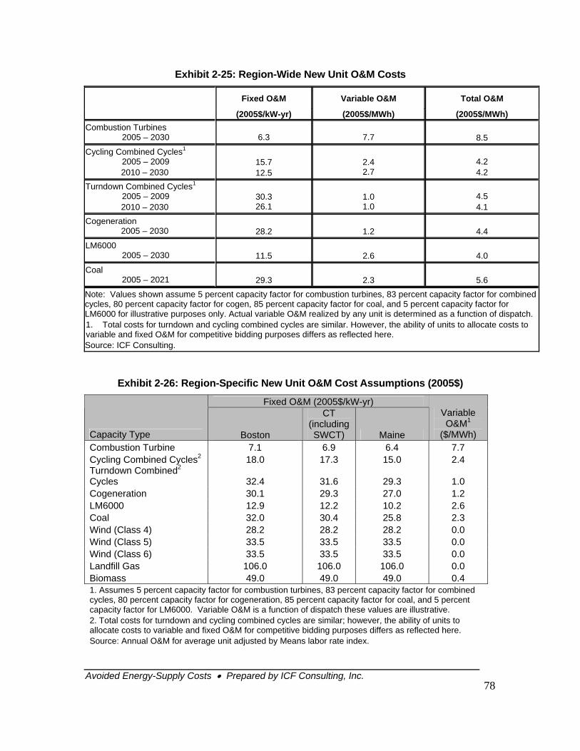
Avoided Energy-Supply Costs • Prepared by ICF Consulting, Inc.
78
Exhibit 2-25: Region-Wide New Unit O&M Costs
Fixed O&M Variable O&M Total O&M (2005$/kW-yr) (2005$/MWh) (2005$/MWh)
Combustion Turbines 2005 – 2030
6.3
7.7
8.5
Cycling Combined Cycles1 2005 – 2009 2010 – 2030
15.7 12.5
2.4 2.7
4.2 4.2
Turndown Combined Cycles1 2005 – 2009 2010 – 2030
30.3 26.1
1.0 1.0
4.5 4.1
Cogeneration 2005 – 2030
28.2
1.2
4.4
LM6000 2005 – 2030
11.5
2.6
4.0
Coal 2005 – 2021
29.3
2.3
5.6
Note: Values shown assume 5 percent capacity factor for combustion turbines, 83 percent capacity factor for combined cycles, 80 percent capacity factor for cogen, 85 percent capacity factor for coal, and 5 percent capacity factor for LM6000 for illustrative purposes only. Actual variable O&M realized by any unit is determined as a function of dispatch. 1. Total costs for turndown and cycling combined cycles are similar. However, the ability of units to allocate costs to variable and fixed O&M for competitive bidding purposes differs as reflected here. Source: ICF Consulting.
Exhibit 2-26: Region-Specific New Unit O&M Cost Assumptions (2005$)
Fixed O&M (2005$/kW-yr)
Capacity Type Boston
CT (including SWCT) Maine
Variable O&M1
($/MWh) Combustion Turbine 7.1 6.9 6.4 7.7 Cycling Combined Cycles2 18.0 17.3 15.0 2.4 Turndown Combined2 Cycles 32.4 31.6 29.3 1.0 Cogeneration 30.1 29.3 27.0 1.2 LM6000 12.9 12.2 10.2 2.6 Coal 32.0 30.4 25.8 2.3 Wind (Class 4) 28.2 28.2 28.2 0.0 Wind (Class 5) 33.5 33.5 33.5 0.0 Wind (Class 6) 33.5 33.5 33.5 0.0 Landfill Gas 106.0 106.0 106.0 0.0 Biomass 49.0 49.0 49.0 0.4 1. Assumes 5 percent capacity factor for combustion turbines, 83 percent capacity factor for combined cycles, 80 percent capacity factor for cogeneration, 85 percent capacity factor for coal, and 5 percent capacity factor for LM6000. Variable O&M is a function of dispatch these values are illustrative. 2. Total costs for turndown and cycling combined cycles are similar; however, the ability of units to allocate costs to variable and fixed O&M for competitive bidding purposes differs as reflected here. Source: Annual O&M for average unit adjusted by Means labor rate index.
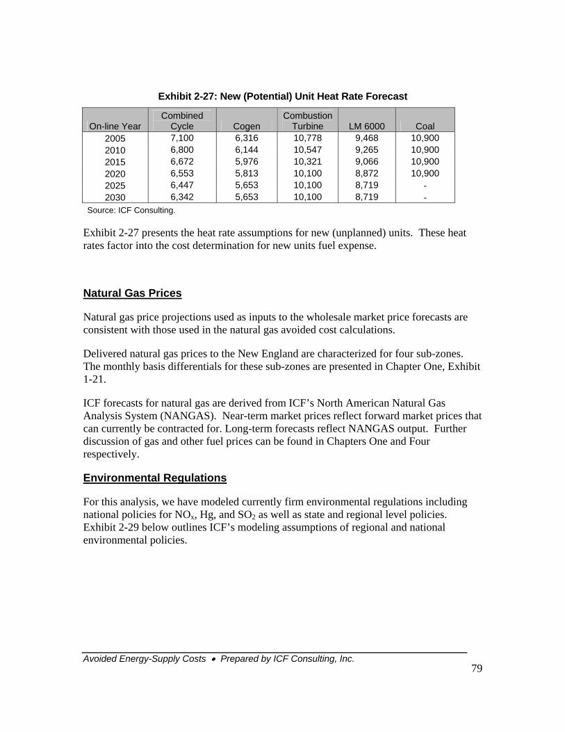
Avoided Energy-Supply Costs • Prepared by ICF Consulting, Inc.
79
Exhibit 2-27: New (Potential) Unit Heat Rate Forecast
On-line Year Combined
Cycle Cogen Combustion
Turbine LM 6000 Coal 2005 7,100 6,316 10,778 9,468 10,900 2010 6,800 6,144 10,547 9,265 10,900 2015 6,672 5,976 10,321 9,066 10,900 2020 6,553 5,813 10,100 8,872 10,900 2025 6,447 5,653 10,100 8,719 - 2030 6,342 5,653 10,100 8,719 -
Source: ICF Consulting.
Exhibit 2-27 presents the heat rate assumptions for new (unplanned) units. These heat rates factor into the cost determination for new units fuel expense.
Natural Gas Prices
Natural gas price projections used as inputs to the wholesale market price forecasts are consistent with those used in the natural gas avoided cost calculations.
Delivered natural gas prices to the New England are characterized for four sub-zones. The monthly basis differentials for these sub-zones are presented in Chapter One, Exhibit 1-21.
ICF forecasts for natural gas are derived from ICF’s North American Natural Gas Analysis System (NANGAS). Near-term market prices reflect forward market prices that can currently be contracted for. Long-term forecasts reflect NANGAS output. Further discussion of gas and other fuel prices can be found in Chapters One and Four respectively.
Environmental Regulations
For this analysis, we have modeled currently firm environmental regulations including national policies for NOx, Hg, and SO2 as well as state and regional level policies. Exhibit 2-29 below outlines ICF’s modeling assumptions of regional and national environmental policies.
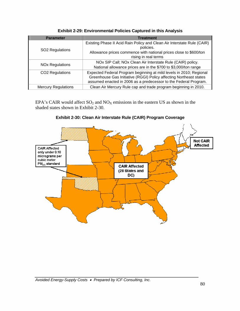
Avoided Energy-Supply Costs • Prepared by ICF Consulting, Inc.
80
Exhibit 2-29: Environmental Policies Captured in this Analysis Parameter Treatment
SO2 Regulations
Existing Phase II Acid Rain Policy and Clean Air Interstate Rule (CAIR) policies.
Allowance prices commence with national prices close to $600/ton rising in real terms
NOx Regulations NOx SIP Call; NOx Clean Air Interstate Rule (CAIR) policy. National allowance prices are in the $700 to $3,000/ton range
CO2 Regulations Expected Federal Program beginning at mild levels in 2010; Regional Greenhouse Gas Initiative (RGGI) Policy affecting Northeast states
assumed enacted in 2006 as a predecessor to the Federal Program. Mercury Regulations Clean Air Mercury Rule cap and trade program beginning in 2010.
EPA’s CAIR would affect SO2 and NOX emissions in the eastern US as shown in the shaded states shown in Exhibit 2-30.
Exhibit 2-30: Clean Air Interstate Rule (CAIR) Program Coverage
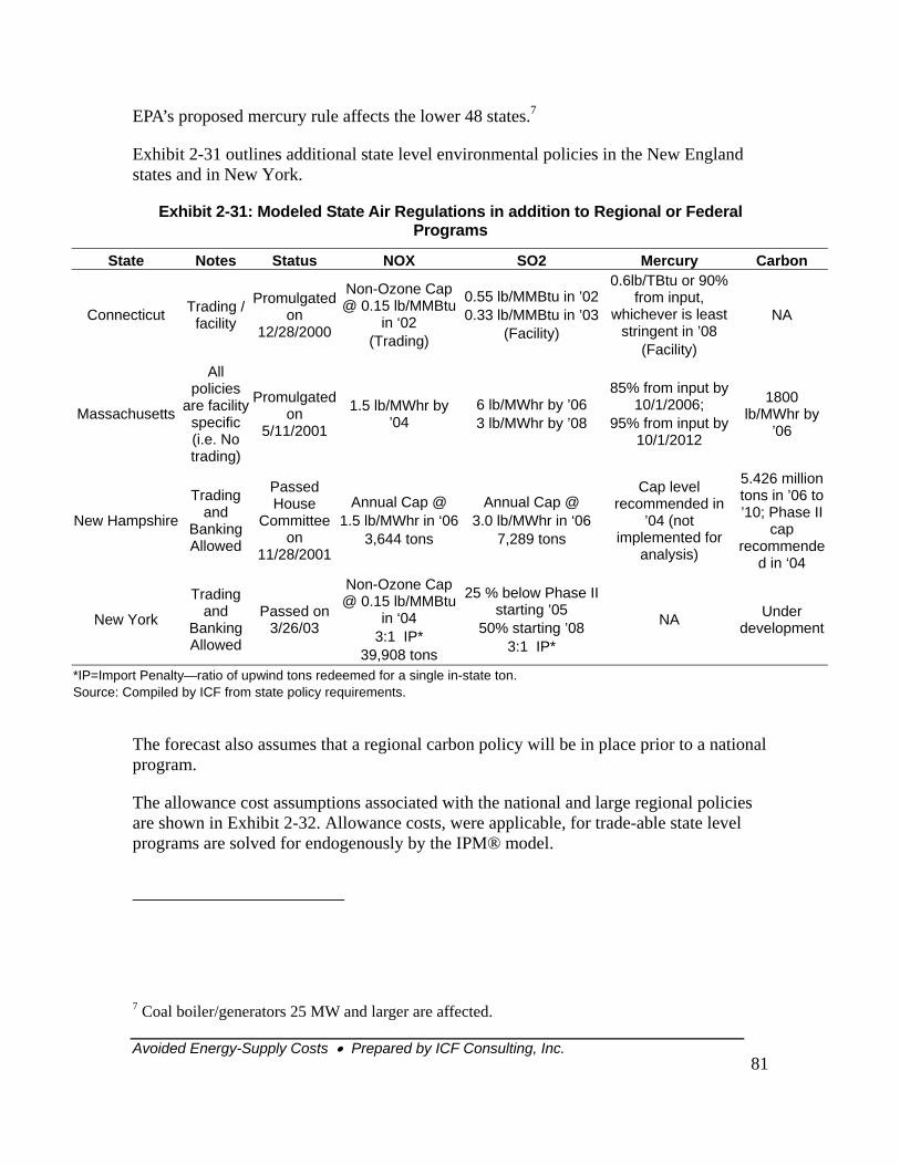
Avoided Energy-Supply Costs • Prepared by ICF Consulting, Inc.
81
EPA’s proposed mercury rule affects the lower 48 states.7
Exhibit 2-31 outlines additional state level environmental policies in the New England states and in New York.
Exhibit 2-31: Modeled State Air Regulations in addition to Regional or Federal Programs
State Notes Status NOX SO2 Mercury Carbon
Connecticut Trading / facility
Promulgated on
12/28/2000
Non-Ozone Cap @ 0.15 lb/MMBtu
in ‘02 (Trading)
0.55 lb/MMBtu in ’020.33 lb/MMBtu in ’03
(Facility)
0.6lb/TBtu or 90% from input,
whichever is least stringent in ’08
(Facility)
NA
Massachusetts
All policies
are facility specific (i.e. No trading)
Promulgated on
5/11/2001
1.5 lb/MWhr by ’04
6 lb/MWhr by ’06 3 lb/MWhr by ’08
85% from input by 10/1/2006;
95% from input by 10/1/2012
1800 lb/MWhr by
’06
New Hampshire
Trading and
Banking Allowed
Passed House
Committee on
11/28/2001
Annual Cap @ 1.5 lb/MWhr in ‘06
3,644 tons
Annual Cap @ 3.0 lb/MWhr in ‘06
7,289 tons
Cap level recommended in
’04 (not implemented for
analysis)
5.426 million tons in ’06 to ’10; Phase II
cap recommende
d in ‘04
New York
Trading and
Banking Allowed
Passed on 3/26/03
Non-Ozone Cap @ 0.15 lb/MMBtu
in ‘04 3:1 IP*
39,908 tons
25 % below Phase II starting ’05
50% starting ’08 3:1 IP*
NA Under development
*IP=Import Penalty—ratio of upwind tons redeemed for a single in-state ton. Source: Compiled by ICF from state policy requirements.
The forecast also assumes that a regional carbon policy will be in place prior to a national program.
The allowance cost assumptions associated with the national and large regional policies are shown in Exhibit 2-32. Allowance costs, were applicable, for trade-able state level programs are solved for endogenously by the IPM® model.
7 Coal boiler/generators 25 MW and larger are affected.
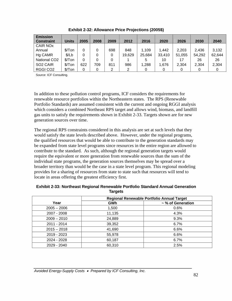
Avoided Energy-Supply Costs • Prepared by ICF Consulting, Inc.
82
Exhibit 2-32: Allowance Price Projections (2005$) Emission Constraint Units 2005 2008 2009 2012 2016 2020 2026 2030 2040 CAIR NOx Annual $/Ton 0 0 698 848 1,109 1,442 2,203 2,436 3,132 Hg CAMR $/Lb 0 0 0 19,629 25,684 33,410 51,055 54,292 62,644 National CO2 $/Ton 0 0 0 1 5 10 17 26 26 SO2 CAIR $/Ton 622 709 811 986 1,288 1,676 2,304 2,304 2,304 RGGI CO2 $/Ton 0 0 2 2 0 0 0 0 0 Source: ICF Consulting.
In addition to these pollution control programs, ICF considers the requirements for renewable resource portfolios within the Northeastern states. The RPS (Renewable Portfolio Standards) are assumed consistent with the current and ongoing RGGI analysis which considers a combined Northeast RPS target and allows wind, biomass, and landfill gas units to satisfy the requirements shown in Exhibit 2-33. Targets shown are for new generation sources over time.
The regional RPS constraints considered in this analysis are set at such levels that they would satisfy the state levels described above. However, under the regional programs, the qualified resources that would be able to contribute to the generation standards may be expanded from state level programs since resources in the entire region are allowed to contribute to the standard. As such, although the regional generation targets would require the equivalent or more generation from renewable sources than the sum of the individual state programs, the generation sources themselves may be spread over a broader territory than would be the case in a state level program. This regional modeling provides for a sharing of resources from state to state such that resources will tend to locate in areas offering the greatest efficiency first.
Exhibit 2-33: Northeast Regional Renewable Portfolio Standard Annual Generation Targets
Regional Renewable Portfolio Annual Target Year GWh ~ % of Generation
2005 – 2006 1,500 0.6% 2007 - 2008 11,135 4.3% 2009 – 2010 24,889 9.3% 2011 - 2014 39,352 6.7% 2015 – 2018 41,690 6.6% 2019 - 2023 55,978 6.6% 2024 - 2028 60,187 6.7% 2029 - 2040 60,310 2.5%
Avoided Energy-Supply Costs • Prepared by ICF Consulting, Inc.
83
Transmission Inter-Regional Transmission
New England is directly interconnected with the New York ISO (NYISO) and New Brunswick and has a DC tie with Quebec. Transmission limits reflect the New England RTEP, ICF AC load flow studies, and NERC studies.
The primary physical interconnections between New England and neighboring systems consist of:
• Two high voltage DC interconnections with Hydro Quebec (Highgate and Phase II)
• One 345 kV interconnection with New Brunswick
• Two 345 kV interconnections with ISO-NY
• Cross Sound Cable interconnection with ISO-NY (LIPA)
New England as a whole can import up to roughly 17 percent of its peak demand through its external interconnections. Similarly, New England can export up to 14 percent of its peak demand.
Hydro Quebec has historically been a low-cost power provider to the New England market interconnecting through both Vermont and Central Massachusetts. Vermont has the capability to import or export 225 MW of capacity in the summer and 67.5 MW of capacity in the winter with Hydro Quebec. Central Massachusetts has a total import/export capability of 1500 MW of capacity in the summer and 450 MW of capacity in the winter with Hydro Quebec.
New Brunswick is more remote, interconnecting only through Maine, and has a more limited transfer capacity. The Maine to New Brunswick interconnection allows for movement of 700 MW of capacity in the summer and 210 MW of capacity in the winter.
The new 330 MW high voltage direct current (HVDC) transmission interconnection between New Haven, CT and Shoreham, NY has been completed and is energized. As part of the approval process for the Cross Sound Cable, a new transmission line (“1385”) connecting Long Island and Norwalk is also anticipated to be complete by the summer of 2008. This new line replaces an existing line that has been leaking coolant oil.
Avoided Energy-Supply Costs • Prepared by ICF Consulting, Inc.
84
Intra-Regional Transmission
ISO New England’s annual transmission plan, the Regional Transmission Expansion Planning (RTEP) study, released in 20048, found that almost 600 million dollars in transmission upgrades might be needed to maintain power system reliability and improve wholesale electricity market efficiency. The study concludes that southwest Connecticut is currently the largest area of concern, but transmission congestion also now exists in northwestern Vermont because of a lack of power plants in the area and weak transmission links. The RTEP 2004 proposed transmission projects in these two areas represent approximately $400 million in infrastructure investment. Current estimates for Southwest Connecticut (Phase I and Phase II) are now estimated at closer to $1 billion.
The major internal transmission lines within New England are shown in Exhibit 2-34 (Exhibit 2-17 presents zonal transfer limitations).
8 RSP 2005 has been released but the modeling for this study was completed well before the release of the new report.
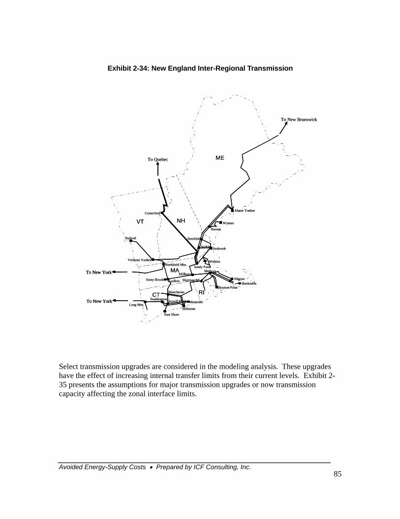
Avoided Energy-Supply Costs • Prepared by ICF Consulting, Inc.
85
Exhibit 2-34: New England Inter-Regional Transmission
Select transmission upgrades are considered in the modeling analysis. These upgrades have the effect of increasing internal transfer limits from their current levels. Exhibit 2-35 presents the assumptions for major transmission upgrades or now transmission capacity affecting the zonal interface limits.
NH
ME
VT
MA
CT RI
Sandy Pond
Comerford
To Quebec
Maine Yankee
Buxton
Deerfield
Scobie Seabrook
Vermont Yankee
Rutland
Northfield Mtn.
To New York
LudlowStony Brook
Manchester
Millstone
East Shore
Southington Scovill Rock
Sherman Rd.
Brayton Point
PilgrimBarnstable
MedwayMillbury
Woburn
Wyman
Long Mtn.Montville
To New Brunswick
To New York
NH
ME
VT
MA
CT RI
Sandy Pond
Comerford
To Quebec
Maine Yankee
Buxton
Deerfield
Scobie Seabrook
Vermont Yankee
Rutland
Northfield Mtn.
To New YorkTo New York
LudlowStony Brook
Manchester
Millstone
East Shore
Southington Scovill Rock
Sherman Rd.
Brayton Point
PilgrimBarnstable
MedwayMillbury
Woburn
Wyman
Long Mtn.Montville
To New Brunswick
To New YorkTo New York
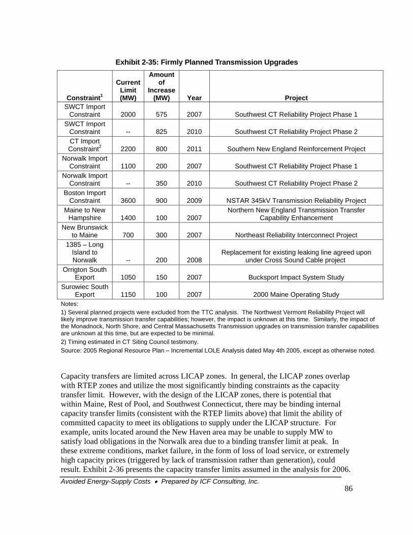
Avoided Energy-Supply Costs • Prepared by ICF Consulting, Inc.
86
Exhibit 2-35: Firmly Planned Transmission Upgrades
Constraint1
Current Limit (MW)
Amount of
Increase (MW) Year Project
SWCT Import Constraint 2000 575 2007 Southwest CT Reliability Project Phase 1
SWCT Import Constraint -- 825 2010 Southwest CT Reliability Project Phase 2 CT Import Constraint2 2200 800 2011 Southern New England Reinforcement Project
Norwalk Import Constraint 1100 200 2007 Southwest CT Reliability Project Phase 1
Norwalk Import Constraint -- 350 2010 Southwest CT Reliability Project Phase 2
Boston Import Constraint 3600 900 2009 NSTAR 345kV Transmission Reliability Project
Maine to New Hampshire 1400 100 2007
Northern New England Transmission Transfer Capability Enhancement
New Brunswick to Maine 700 300 2007 Northeast Reliability Interconnect Project
1385 – Long Island to Norwalk -- 200 2008
Replacement for existing leaking line agreed upon under Cross Sound Cable project
Orrigton South Export 1050 150 2007 Bucksport Impact System Study
Surowiec South Export 1150 100 2007 2000 Maine Operating Study
Notes: 1) Several planned projects were excluded from the TTC analysis. The Northwest Vermont Reliability Project will likely improve transmission transfer capabilities; however, the impact is unknown at this time. Similarly, the impact of the Monadnock, North Shore, and Central Massachusetts Transmission upgrades on transmission transfer capabilities are unknown at this time, but are expected to be minimal. 2) Timing estimated in CT Siting Council testimony. Source: 2005 Regional Resource Plan – Incremental LOLE Analysis dated May 4th 2005, except as otherwise noted.
Capacity transfers are limited across LICAP zones. In general, the LICAP zones overlap with RTEP zones and utilize the most significantly binding constraints as the capacity transfer limit. However, with the design of the LICAP zones, there is potential that within Maine, Rest of Pool, and Southwest Connecticut, there may be binding internal capacity transfer limits (consistent with the RTEP limits above) that limit the ability of committed capacity to meet its obligations to supply under the LICAP structure. For example, units located around the New Haven area may be unable to supply MW to satisfy load obligations in the Norwalk area due to a binding transfer limit at peak. In these extreme conditions, market failure, in the form of loss of load service, or extremely high capacity prices (triggered by lack of transmission rather than generation), could result. Exhibit 2-36 presents the capacity transfer limits assumed in the analysis for 2006.
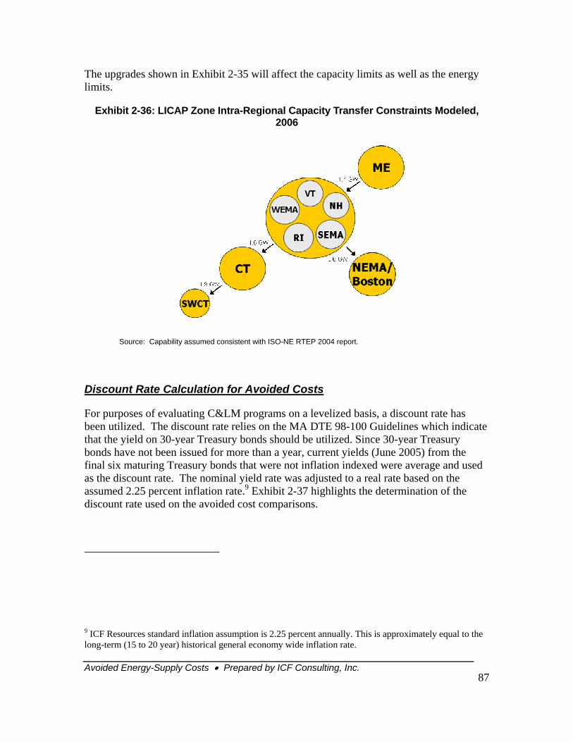
Avoide
The upgrades shown in Exhibit 2-35 will affect the capacity limits as well as the energy limits.
Exhibit 2-36: LICAP Zone Intra-Regional Capacity Transfer Constraints Modeled, 2006
Disco
For pubeen uthat thbonds final sias the assumediscou
9 ICF Rlong-ter
.
Source: Capability assumed consistent with ISO-NE RTEP 2004 reportd Energy-Supply Costs • Prepared by ICF Consulting, Inc. 87
unt Rate Calculation for Avoided Costs
rposes of evaluating C&LM programs on a levelized basis, a discount rate has tilized. The discount rate relies on the MA DTE 98-100 Guidelines which indicate e yield on 30-year Treasury bonds should be utilized. Since 30-year Treasury have not been issued for more than a year, current yields (June 2005) from the x maturing Treasury bonds that were not inflation indexed were average and used discount rate. The nominal yield rate was adjusted to a real rate based on the d 2.25 percent inflation rate.9 Exhibit 2-37 highlights the determination of the
nt rate used on the avoided cost comparisons.
esources standard inflation assumption is 2.25 percent annually. This is approximately equal to the m (15 to 20 year) historical general economy wide inflation rate.
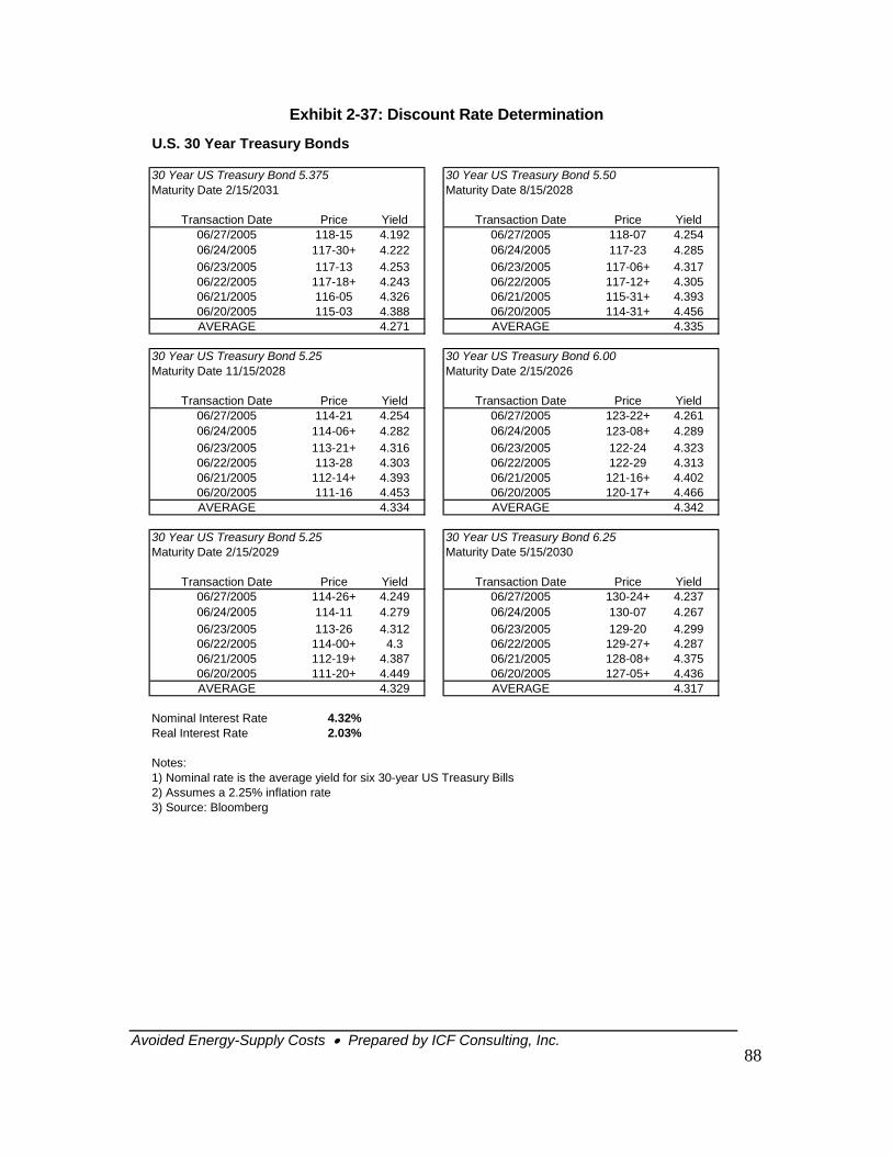
Avoided Energy-Supply Costs • Prepared by ICF Consulting, Inc.
88
Exhibit 2-37: Discount Rate Determination
U.S. 30 Year Treasury Bonds
30 Year US Treasury Bond 5.375 30 Year US Treasury Bond 5.50Maturity Date 2/15/2031 Maturity Date 8/15/2028
Transaction Date Price Yield Transaction Date Price Yield06/27/2005 118-15 4.192 06/27/2005 118-07 4.25406/24/2005 117-30+ 4.222 06/24/2005 117-23 4.28506/23/2005 117-13 4.253 06/23/2005 117-06+ 4.31706/22/2005 117-18+ 4.243 06/22/2005 117-12+ 4.30506/21/2005 116-05 4.326 06/21/2005 115-31+ 4.39306/20/2005 115-03 4.388 06/20/2005 114-31+ 4.456AVERAGE 4.271 AVERAGE 4.335
30 Year US Treasury Bond 5.25 30 Year US Treasury Bond 6.00Maturity Date 11/15/2028 Maturity Date 2/15/2026
Transaction Date Price Yield Transaction Date Price Yield06/27/2005 114-21 4.254 06/27/2005 123-22+ 4.26106/24/2005 114-06+ 4.282 06/24/2005 123-08+ 4.28906/23/2005 113-21+ 4.316 06/23/2005 122-24 4.32306/22/2005 113-28 4.303 06/22/2005 122-29 4.31306/21/2005 112-14+ 4.393 06/21/2005 121-16+ 4.40206/20/2005 111-16 4.453 06/20/2005 120-17+ 4.466AVERAGE 4.334 AVERAGE 4.342
30 Year US Treasury Bond 5.25 30 Year US Treasury Bond 6.25Maturity Date 2/15/2029 Maturity Date 5/15/2030
Transaction Date Price Yield Transaction Date Price Yield06/27/2005 114-26+ 4.249 06/27/2005 130-24+ 4.23706/24/2005 114-11 4.279 06/24/2005 130-07 4.26706/23/2005 113-26 4.312 06/23/2005 129-20 4.29906/22/2005 114-00+ 4.3 06/22/2005 129-27+ 4.28706/21/2005 112-19+ 4.387 06/21/2005 128-08+ 4.37506/20/2005 111-20+ 4.449 06/20/2005 127-05+ 4.436AVERAGE 4.329 AVERAGE 4.317
Nominal Interest Rate 4.32%Real Interest Rate 2.03%
Notes: 1) Nominal rate is the average yield for six 30-year US Treasury Bills2) Assumes a 2.25% inflation rate3) Source: Bloomberg
Avoided Energy-Supply Costs • Prepared by ICF Consulting, Inc.
89
Chapter Three: Avoided Electric Supply Component Cost Forecast Results The avoided electric supply costs to be used in conservation and load management (C&LM) cost-effectiveness analyses are comprised of three main components: (1) wholesale energy supply costs, (2) wholesale capacity supply costs (both of which are tied to the costs of operating and maintaining power generators), and (3) out-of-market supply costs associated with system reliability or congestion.10 In addition to these components, certain transmission and distribution investments may be avoidable and additional benefits may be derived from price responsiveness to demand reduction. These additional elements are presented in Chapters 5 and 6.
Using the assumptions discussed in Chapter Two of this report, ICF developed a forecast for each of the three main components for each of the AESC screening zones identified in Exhibit 3-1. The AESC screening zones were identified by the sponsors and vary from the ISO-NE Pricing, RTEP, and LICAP zonal definitions also shown in Exhibit 3-1. This chapter provides summary results for the three component costs at the AESC screening zone level for reference purposes only. Full results for use in the AESC screening tools including a breakout by alternate zones and supplemental information on the component costs are provided in Appendix 2 and have also been provided to the Study Group in spreadsheet format.
Appendix 2 also provides definitional information for the parameters presented in the spreadsheet results and should be referred to as a guide to help interpret and use the results. All values are presented in real 2005$ unless otherwise noted.
10 Out-of-market costs reflect RMR payments as discussed in Chapter Two. To qualify for these payments, a generator must be shown to be required to be on-line for an adequate reliability level to be maintained on the electric grid; hence the generator is valued for its capacity. These payments typically reflect a traditional cost-of-service recovery based on a regulated rate of return. A generator receiving these payments will recover full costs (variable and fixed) plus some allowed rate of return.
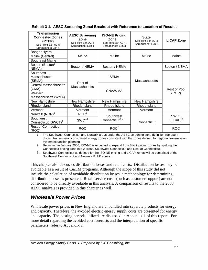
Avoided Energy-Supply Costs • Prepared by ICF Consulting, Inc.
90
Exhibit 3-1. AESC Screening Zonal Breakout with Reference to Location of Results
Transmission Congested Zones
(RTEP) See Text Exh A2-5 Spreadsheet Exh 4
AESC Screening Zone
See Text Exh A2-2 Spreadsheet Exh 1
ISO-NE Pricing Zone
See Text Exh A2-4 Spreadsheet Exh 3
State See Text Exh A2-3 Spreadsheet Exh 2
LICAP Zone
Bangor Hydro Maine (Central) Southeast Maine
Maine Maine Maine Maine
Boston (Boston/ NEMA) Boston / NEMA Boston / NEMA Boston / NEMA
Southeast Massachusetts (SEMA)
SEMA
Central Massachusetts (CMA) Western Massachusetts (WMA)
Rest of Massachusetts
CNA/WMA
Massachusetts
New Hampshire New Hampshire New Hampshire New Hampshire Rhode Island Rhode Island Rhode Island Rhode Island Vermont Vermont Vermont Vermont
Rest of Pool (ROP)
Norwalk (NOR)1 NOR1
Southwest Connecticut (SWCT)1 SWCT1
Southwest Connecticut2. 3
SWCT (LICAP)3
Rest of Connecticut (ROC) ROC ROC2
Connecticut
ROC
1. The Southwest Connecticut and Norwalk areas under the AESC screening zone definition represent distinct transmission constrained energy zones consistent with the zones defined for regional transmission system expansion planning.
2. Beginning in January 2006, ISO-NE is expected to expand from 8 to 9 pricing zones by splitting the Connecticut pricing zone into 2 areas, Southwest Connecticut and Rest of Connecticut.
3. Southwest Connecticut as defined for the ISO-NE pricing and LICAP zones will be comprised of the Southwest Connecticut and Norwalk RTEP zones.
This chapter also discusses distribution losses and retail costs. Distribution losses may be avoidable as a result of C&LM programs. Although the scope of this study did not include the calculation of avoidable distribution losses, a methodology for determining distribution losses is presented. Retail service costs (such as customer support) are not considered to be directly avoidable in this analysis. A comparison of results to the 2003 AESC analysis is provided in this chapter as well.
Wholesale Power Prices
Wholesale power prices in New England are unbundled into separate products for energy and capacity. Therefore, the avoided electric energy supply costs are presented for energy and capacity. The costing periods utilized are discussed in Appendix 1 of this report. For more detail regarding the avoided cost forecasts and the interpretation of specific parameters, refer to Appendix 2.
Avoided Energy-Supply Costs • Prepared by ICF Consulting, Inc.
91
Avoided Energy Supply Costs
Marginal energy prices in New England are largely driven by gas-fired generating resources, particularly in the near-term. A large amount of combined cycle generation is available in the market and these resources tend to set prices in most hours. Higher cost oil and gas steam generation units will often be the marginal resource in higher priced peak-hours. This analysis reflects the post-Katrina natural gas price forecast presented in Chapter One of this report. All modeling analysis was completed in July prior to the impact of Katrina on fuel prices. In order to capture the impact of Katrina, an offline adjustment was made to the energy price forecasts for the near-term (the adjusted forecast period). To make this adjustment, the initial implied heat rate for peak and off-peak periods (which reflected use of gas resources on the margin) resulting from the model were kept constant and the energy price was recalculated using the revised gas delivered gas price forecast. Exhibit 3-2 reflects the post-Katrina11 electric energy forecasts. This exhibit is a summary of the energy component price forecast for illustration and comparison purposes, and is not intended for use in cost-effectiveness analysis screening.
Beginning in the mid-term, new unit efficiency and environmental policies begin to affect marginal prices. The average efficiency of gas-fired capacity improves as new gas-fired units come online to meet growing demand, resulting in downward pressure on the implied heat rate and energy prices. Simultaneously, environmental polices become more stringent and have higher compliance costs. The higher environmental costs push energy prices upwards.
11 The impact of Katrina on fuel prices was assumed to affect only the electric energy values. The electric capacity values were assumed to be unaffected given that fuel price impact did not affect the long-term and would be unlikely to affect capacity entry and exit decisions.
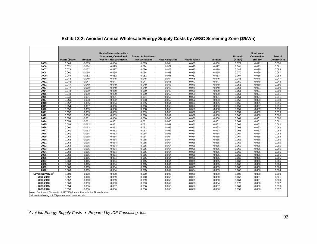
Exhibit 3-2: Avoided Annual Wholesale Energy Supply Costs by AESC Screening Zone ($/kWh)
Maine (State) Boston
Rest of Massachusetts - Southeast, Central and Western Massachusetts
Boston & Southeast Massachusetts New Hampshire Rhode Island Vermont
Norwalk (RTEP)
Southwest Connecticut
(RTEP)Rest of
Connecticut 2005 0.063 0.065 0.066 0.065 0.064 0.065 0.068 0.073 0.072 0.0702006 0.071 0.074 0.075 0.074 0.072 0.075 0.077 0.084 0.083 0.0812007 0.073 0.077 0.077 0.076 0.075 0.077 0.079 0.087 0.085 0.0842008 0.061 0.065 0.065 0.064 0.063 0.065 0.065 0.070 0.069 0.0672009 0.049 0.052 0.052 0.052 0.051 0.052 0.053 0.057 0.055 0.0542010 0.043 0.045 0.045 0.045 0.044 0.045 0.046 0.048 0.048 0.0472011 0.045 0.047 0.047 0.047 0.046 0.047 0.047 0.050 0.049 0.0482012 0.047 0.049 0.049 0.049 0.048 0.049 0.049 0.051 0.050 0.0502013 0.047 0.050 0.049 0.049 0.049 0.049 0.049 0.051 0.051 0.0502014 0.048 0.050 0.050 0.050 0.049 0.050 0.050 0.051 0.051 0.0502015 0.048 0.050 0.050 0.050 0.050 0.050 0.050 0.051 0.051 0.0512016 0.048 0.051 0.051 0.051 0.050 0.050 0.051 0.051 0.051 0.0512017 0.050 0.053 0.052 0.053 0.052 0.052 0.053 0.053 0.053 0.0532018 0.052 0.055 0.054 0.055 0.054 0.054 0.055 0.055 0.055 0.0552019 0.054 0.057 0.056 0.056 0.056 0.056 0.056 0.057 0.057 0.0562020 0.056 0.059 0.058 0.058 0.058 0.058 0.058 0.059 0.059 0.0582021 0.057 0.059 0.059 0.059 0.058 0.059 0.059 0.059 0.059 0.0592022 0.057 0.060 0.059 0.060 0.059 0.059 0.060 0.060 0.060 0.0602023 0.058 0.061 0.060 0.060 0.060 0.060 0.060 0.061 0.061 0.0602024 0.059 0.061 0.061 0.061 0.060 0.061 0.061 0.061 0.061 0.0612025 0.059 0.062 0.061 0.062 0.061 0.061 0.062 0.062 0.062 0.0622026 0.060 0.063 0.062 0.062 0.062 0.062 0.063 0.063 0.063 0.0622027 0.061 0.063 0.062 0.063 0.062 0.063 0.063 0.063 0.063 0.0632028 0.061 0.064 0.063 0.064 0.063 0.064 0.064 0.064 0.064 0.0632029 0.062 0.065 0.064 0.064 0.064 0.064 0.065 0.064 0.065 0.0642030 0.063 0.066 0.064 0.065 0.064 0.065 0.065 0.065 0.065 0.0652031 0.063 0.065 0.064 0.065 0.064 0.065 0.065 0.065 0.065 0.0652032 0.063 0.065 0.064 0.065 0.064 0.065 0.065 0.065 0.065 0.0652033 0.063 0.065 0.064 0.065 0.064 0.065 0.065 0.065 0.065 0.0652034 0.063 0.065 0.064 0.065 0.064 0.065 0.065 0.065 0.065 0.0652035 0.063 0.065 0.064 0.065 0.064 0.065 0.065 0.066 0.065 0.0652036 0.063 0.065 0.064 0.065 0.064 0.065 0.065 0.066 0.065 0.0652037 0.063 0.065 0.064 0.065 0.064 0.065 0.065 0.066 0.066 0.0652038 0.063 0.065 0.064 0.065 0.064 0.065 0.065 0.066 0.066 0.0642039 0.063 0.065 0.064 0.065 0.064 0.065 0.065 0.066 0.066 0.0642040 0.063 0.065 0.064 0.065 0.064 0.064 0.065 0.066 0.066 0.064
Levelized Values1 0.000 0.000 0.000 0.000 0.000 0.000 0.000 0.000 0.000 0.0002005-2040 0.057 0.060 0.059 0.060 0.059 0.059 0.060 0.062 0.061 0.0612006-2040 0.057 0.060 0.059 0.059 0.059 0.059 0.060 0.061 0.061 0.0602006-2010 0.060 0.063 0.063 0.063 0.062 0.063 0.064 0.070 0.068 0.0672006-2015 0.054 0.056 0.057 0.056 0.055 0.056 0.057 0.061 0.060 0.0592006-2020 0.053 0.056 0.056 0.056 0.055 0.056 0.056 0.059 0.058 0.057
Note: Southwest Connecticut (RTEP) does not include the Norwalk area.1) Levelized using a 2.03 percent real discount rate
Avoided Energy-Supply Costs • Prepared by ICF Consulting, Inc.
92

Avoided Energy-Supply Costs • Prepared by ICF Consulting, Inc.
93
On a zonal level, in the near-term, energy prices are higher in the import constrained regions of Norwalk, Southwest Connecticut and Norwalk. Overall, prices also tend to be higher in zones west of the East/West constraint12.
Avoided Capacity Supply Costs
Capacity prices in the forecast reflect the assumption that a LICAP market structure will exist going forward13. Transmission constraints contribute to capacity value under LICAP. Locational value is created due to transmission constraints. In the most extreme cases, constraints will strand megawatts or will isolate load resulting in very low capacity value if the megawatts are stranded or very high capacity value if the load is isolated.
In the near term, much of New England has excess capacity and the locational capacity prices are depressed. Growth in peak demand and new unit costs drive the long-term capacity prices. Over time, as new units are required to serve growing demand, the equilibrium market capacity price will reflect the revenue required by developers to bring new capacity on-line. This revenue requirement reflects the return on and of investment for the developer less any revenues generated in the energy market. As technological improvements occur and the costs of building new units declines in real-terms, the real equilibrium capacity price will decline.
Exhibit 3-3 shows the avoided capacity value by zone—without energy or out-of-market costs. Because of the nature of the capacity market, there is no effect from Hurricane Katrina on the capacity market. Similar to Exhibit 3-2, this exhibit is a summary the capacity component of the price forecast for illustration and comparison purposes, and is not intended for use in cost-effectiveness analysis screening.
12 Refer to Chapter Two Exhibit 2-5.
13 The analysis reflects the assumption that LICAP would begin in January 2006, the proposed start date at the time this study was undertaken. Over the course of the study, delays have resulted in the earliest start date being moved to October 1, 2006. Out-of-market costs were also assumed to be unaffected, as fuel costs would be considered to be recoverable in the energy dispatch of the units driving out-of-market costs.
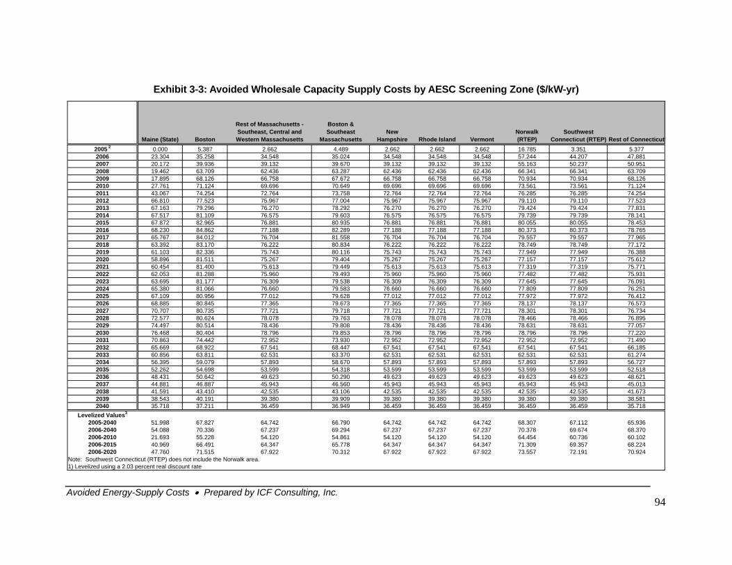
Exhibit 3-3: Avoided Wholesale Capacity Supply Costs by AESC Screening Zone ($/kW-yr)
Maine (State) Boston
Rest of Massachusetts - Southeast, Central and Western Massachusetts
Boston & Southeast
MassachusettsNew
Hampshire Rhode Island VermontNorwalk (RTEP)
Southwest Connecticut (RTEP) Rest of Connecticut
2005 2 0.000 5.387 2.662 4.489 2.662 2.662 2.662 16.785 3.351 5.3772006 23.304 35.258 34.548 35.024 34.548 34.548 34.548 57.244 44.207 47.8812007 20.172 39.936 39.132 39.670 39.132 39.132 39.132 55.163 50.237 50.9512008 19.462 63.709 62.436 63.287 62.436 62.436 62.436 66.341 66.341 63.7092009 17.895 68.126 66.758 67.672 66.758 66.758 66.758 70.934 70.934 68.1262010 27.761 71.124 69.696 70.649 69.696 69.696 69.696 73.561 73.561 71.1242011 43.067 74.254 72.764 73.758 72.764 72.764 72.764 76.285 76.285 74.2542012 66.810 77.523 75.967 77.004 75.967 75.967 75.967 79.110 79.110 77.5232013 67.163 79.296 76.270 78.292 76.270 76.270 76.270 79.424 79.424 77.8312014 67.517 81.109 76.575 79.603 76.575 76.575 76.575 79.739 79.739 78.1412015 67.872 82.965 76.881 80.935 76.881 76.881 76.881 80.055 80.055 78.4532016 68.230 84.862 77.188 82.289 77.188 77.188 77.188 80.373 80.373 78.7652017 65.767 84.012 76.704 81.558 76.704 76.704 76.704 79.557 79.557 77.9652018 63.392 83.170 76.222 80.834 76.222 76.222 76.222 78.749 78.749 77.1722019 61.103 82.336 75.743 80.116 75.743 75.743 75.743 77.949 77.949 76.3882020 58.896 81.511 75.267 79.404 75.267 75.267 75.267 77.157 77.157 75.6122021 60.454 81.400 75.613 79.449 75.613 75.613 75.613 77.319 77.319 75.7712022 62.053 81.288 75.960 79.493 75.960 75.960 75.960 77.482 77.482 75.9312023 63.695 81.177 76.309 79.538 76.309 76.309 76.309 77.645 77.645 76.0912024 65.380 81.066 76.660 79.583 76.660 76.660 76.660 77.809 77.809 76.2512025 67.109 80.956 77.012 79.628 77.012 77.012 77.012 77.972 77.972 76.4122026 68.885 80.845 77.365 79.673 77.365 77.365 77.365 78.137 78.137 76.5732027 70.707 80.735 77.721 79.718 77.721 77.721 77.721 78.301 78.301 76.7342028 72.577 80.624 78.078 79.763 78.078 78.078 78.078 78.466 78.466 76.8952029 74.497 80.514 78.436 79.808 78.436 78.436 78.436 78.631 78.631 77.0572030 76.468 80.404 78.796 79.853 78.796 78.796 78.796 78.796 78.796 77.2202031 70.863 74.442 72.952 73.930 72.952 72.952 72.952 72.952 72.952 71.4902032 65.669 68.922 67.541 68.447 67.541 67.541 67.541 67.541 67.541 66.1852033 60.856 63.811 62.531 63.370 62.531 62.531 62.531 62.531 62.531 61.2742034 56.395 59.079 57.893 58.670 57.893 57.893 57.893 57.893 57.893 56.7272035 52.262 54.698 53.599 54.318 53.599 53.599 53.599 53.599 53.599 52.5182036 48.431 50.642 49.623 50.290 49.623 49.623 49.623 49.623 49.623 48.6212037 44.881 46.887 45.943 46.560 45.943 45.943 45.943 45.943 45.943 45.0132038 41.591 43.410 42.535 43.106 42.535 42.535 42.535 42.535 42.535 41.6732039 38.543 40.191 39.380 39.909 39.380 39.380 39.380 39.380 39.380 38.5812040 35.718 37.211 36.459 36.949 36.459 36.459 36.459 36.459 36.459 35.718
Levelized Values3
2005-2040 51.998 67.827 64.742 66.790 64.742 64.742 64.742 68.307 67.112 65.9362006-2040 54.088 70.336 67.237 69.294 67.237 67.237 67.237 70.378 69.674 68.3702006-2010 21.693 55.228 54.120 54.861 54.120 54.120 54.120 64.454 60.736 60.1022006-2015 40.969 66.491 64.347 65.778 64.347 64.347 64.347 71.309 69.357 68.2242006-2020 47.760 71.515 67.922 70.312 67.922 67.922 67.922 73.557 72.191 70.924
Note: Southwest Connecticut (RTEP) does not include the Norwalk area.1) Levelized using a 2.03 percent real discount rate
Avoided Energy-Supply Costs • Prepared by ICF Consulting, Inc.
94
Avoided Energy-Supply Costs • Prepared by ICF Consulting, Inc.
95
Avoided Out-of-Market Capacity Supply Costs
Out-of-Market avoided capacity supply costs reflect the costs for maintaining generating units that are not profitable on the electric grid for purposes of reliability. These units are typically identified as Reliability Must Run (RMR) units. The cost recovery requirements were determined in a several step process. First, ICF identified units which under the Reference Case restrictions on retirement and mothballing, were losing money. The additional revenue requirements which would allow these units to break-even were then identified. Finally, the specific situation of the individual units was examined to determine whether those units would qualify for RMR payments. The scope of this analysis did not included detailed voltage or needs assessments that would typically be performed to determine whether a unit qualifies for RMR. Since such detailed modeling was not performed, ICF relied on publicly available information and proprietary power-flow modeling to assess whether units would qualify for RMR. In general, all currently operational generating units in the Norwalk and Southwest Connecticut zones were considered to be required for reliability based on voltage requirements in the Norwalk area. Select areas outside of Norwalk and Southwest Connecticut with known voltage issues also may have RMR units. The New England generating stations which were assigned RMR costs include Bridgeport Energy, Milford, Devon, Kendall Square, Cos Cob, Torrington, Norwalk Harbor, Montville, Mystic, New Boston, Canal, L Street, and Stony Brook. Several units were found to have losses (in some years) but were not considered to qualify for RMR. These include Wyman (which was earlier this year denied a basis for need), Lost Nation, Merrimack, and Flos Inn. Going forward, RMR unit revenue requirements were reduced as the market capacity price increased.
Exhibit 3-4 shows the avoided out-of-market costs by zone—without energy or capacity costs. As with the capacity market, there is no effect from Hurricane Katrina on the out-of-market component of the forecast. Similar to Exhibits 3-2 and 3-3, this exhibit is a summary the out-of-market component of the price forecast for illustration and comparison purposes, and is not intended for use in cost-effectiveness analysis screening.
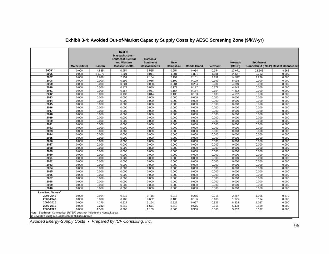
Avoided Energy-Supply Costs • Prepared by ICF Consulting, Inc.
96
Exhibit 3-4: Avoided Out-of-Market Capacity Supply Costs by AESC Screening Zone ($/kW-yr)
Maine (State) Boston
Rest of Massachusetts -
Southeast, Central and Western
Massachusetts
Boston & Southeast
MassachusettsNew
Hampshire Rhode Island VermontNorwalk (RTEP)
Southwest Connecticut (RTEP) Rest of Connecticut
2005 2 0.000 4.835 0.954 3.555 0.954 0.954 0.954 10.071 23.505 8.2652006 0.000 11.077 1.801 8.011 1.801 1.801 1.801 14.667 3.733 0.0002007 0.000 9.630 2.151 7.154 2.151 2.151 2.151 14.312 1.226 0.0002008 0.000 0.000 0.199 0.066 0.199 0.199 0.199 5.035 0.000 0.0002009 0.000 0.000 0.204 0.068 0.204 0.204 0.204 4.889 0.000 0.0002010 0.000 0.000 0.177 0.059 0.177 0.177 0.177 4.645 0.000 0.0002011 0.000 0.000 0.154 0.051 0.154 0.154 0.154 4.412 0.000 0.0002012 0.000 0.000 0.133 0.044 0.133 0.133 0.133 4.192 0.000 0.0002013 0.000 0.000 0.000 0.000 0.000 0.000 0.000 0.000 0.000 0.0002014 0.000 0.000 0.000 0.000 0.000 0.000 0.000 0.000 0.000 0.0002015 0.000 0.000 0.000 0.000 0.000 0.000 0.000 0.000 0.000 0.0002016 0.000 0.000 0.000 0.000 0.000 0.000 0.000 0.000 0.000 0.0002017 0.000 0.000 0.000 0.000 0.000 0.000 0.000 0.000 0.000 0.0002018 0.000 0.000 0.000 0.000 0.000 0.000 0.000 0.000 0.000 0.0002019 0.000 0.000 0.000 0.000 0.000 0.000 0.000 0.000 0.000 0.0002020 0.000 0.000 0.000 0.000 0.000 0.000 0.000 0.000 0.000 0.0002021 0.000 0.000 0.000 0.000 0.000 0.000 0.000 0.000 0.000 0.0002022 0.000 0.000 0.000 0.000 0.000 0.000 0.000 0.000 0.000 0.0002023 0.000 0.000 0.000 0.000 0.000 0.000 0.000 0.000 0.000 0.0002024 0.000 0.000 0.000 0.000 0.000 0.000 0.000 0.000 0.000 0.0002025 0.000 0.000 0.000 0.000 0.000 0.000 0.000 0.000 0.000 0.0002026 0.000 0.000 0.000 0.000 0.000 0.000 0.000 0.000 0.000 0.0002027 0.000 0.000 0.000 0.000 0.000 0.000 0.000 0.000 0.000 0.0002028 0.000 0.000 0.000 0.000 0.000 0.000 0.000 0.000 0.000 0.0002029 0.000 0.000 0.000 0.000 0.000 0.000 0.000 0.000 0.000 0.0002030 0.000 0.000 0.000 0.000 0.000 0.000 0.000 0.000 0.000 0.0002031 0.000 0.000 0.000 0.000 0.000 0.000 0.000 0.000 0.000 0.0002032 0.000 0.000 0.000 0.000 0.000 0.000 0.000 0.000 0.000 0.0002033 0.000 0.000 0.000 0.000 0.000 0.000 0.000 0.000 0.000 0.0002034 0.000 0.000 0.000 0.000 0.000 0.000 0.000 0.000 0.000 0.0002035 0.000 0.000 0.000 0.000 0.000 0.000 0.000 0.000 0.000 0.0002036 0.000 0.000 0.000 0.000 0.000 0.000 0.000 0.000 0.000 0.0002037 0.000 0.000 0.000 0.000 0.000 0.000 0.000 0.000 0.000 0.0002038 0.000 0.000 0.000 0.000 0.000 0.000 0.000 0.000 0.000 0.0002039 0.000 0.000 0.000 0.000 0.000 0.000 0.000 0.000 0.000 0.0002040 0.000 0.000 0.000 0.000 0.000 0.000 0.000 0.000 0.000 0.000
Levelized Values3
2005-2040 0.000 0.964 0.215 0.716 0.215 0.215 0.215 2.287 1.095 0.3192006-2040 0.000 0.808 0.186 0.602 0.186 0.186 0.186 1.975 0.194 0.0002006-2010 0.000 4.270 0.927 3.164 0.927 0.927 0.927 8.828 1.027 0.0002006-2015 0.000 2.242 0.515 1.671 0.515 0.515 0.515 5.478 0.539 0.0002006-2020 0.000 1.568 0.360 1.169 0.360 0.360 0.360 3.832 0.377 0.000
Note: Southwest Connecticut (RTEP) does not include the Norwalk area.1) Levelized using a 2.03 percent real discount rate
Wholesale Price Uncertainties
Uncertainties can and do exist in any forecasting exercise. Given the far reaching assumptions driving the forecast for wholesale power prices, various uncertainties can exist. To minimize the potential for bias towards the assumptions or beliefs of any individual participant in this study, ICF has relied on public sources of information where available. In cases where agreed upon public information was either not available or not reliable; ICF has relied on our own expert judgment. In general, the assumptions rely on a conservative approach to forecasting. Conservative elements of this forecast include:
• Transmission firmly planned upgrades – Rather than relying on a strict rule that transmission upgrades occur only based on those projects already started (ground broken), this forecast includes several announced projects that have a fair likelihood of going forward. These projects include SWCT Phase II; Southern New England Reliability Project (RI-CT); and the Boston/NEMA upgrade. This assumption results in lower wholesale energy and capacity prices than had the strict rule been applied.
• Peak Hour Volatility – All forecast years assume a weather normal pattern and that fuel is readily available. This assumption tends to reduce peak hour volatility which is largely due to weather conditions that vary from normal, fuel shortages or fuel price spikes (also often due to weather). Although average prices may not be affected, this tends to result in a muting of the super-peak period.
• Market Structure – As mentioned earlier, this analysis assumes that for the purposes of setting market clearing prices the market for generation is perfectly competitive and perfectly efficient. Since no market is truly perfectly competitive and efficient, this may either understate or overstate prices, value, and price volatility, all else equal. If sellers have market power, prices may be higher than shown here. This is true of the energy prices which assume bidding at variable cost levels. Likewise capacity markets assume all available capacity in the market contributes to full capability levels with no withholding. Capacity clearing prices may be depressed through the assumption that units may be required to stay on-line for Reliability Must-Run (RMR) reasons. Should these units (which are required to be on-line) be allowed to exit the market, the clearing price of capacity would be above the clearing price determined when these units contribute to the resource mix. That is, should these RMR units exit the market, the market capacity price would be higher since fewer resources would be available. To some extent this effect is corrected for through also capturing the compensation the RMR units receive (above the capacity price) as out-of-market costs.
• Excess Capacity versus Shortages – This analysis assumes any future above-equilibrium prices due to shortages of generation capacity will be exactly offset by periods of excess capacity once the current period of excess capacity ends (i.e. long-term average equilibrium conditions will exist going forward
97
once reached). This is conservative in that one might expect the next phase of the industry cycle to involve shortages and very high prices above equilibrium levels. This would raise value on a present value basis even if it were followed by equal duration and amplitude cycles compared to the current analysis. An even more conservative approach would bias the cycle to even more excess, requiring developers and financiers to be constantly losing money and thus raises issues about the credibility of such a case.
• New Plant Costs and Performance – ICF assumes new plant costs decrease in real terms in later years while their thermal efficiencies improve. This is in spite of the technological challenges to significant future improvements in thermal efficiencies including the effects of extremely high turbine inlet temperature on power plant materials. Thus, future competitors have better performance characteristics. This assumption reduces longer term capacity and energy prices than had technology characteristics been held flat.
• Natural Gas Prices – The analysis herein assumes long-term natural gas prices will return to lower real equilibrium levels well below the currently traded price levels. These forward levels reflect optimistic supply side costs and fully functional economic markets for gas. Recent gas prices have been above the forecast levels. Note this is true of ICF’s post Katrina forecast. Should the recent prices continue forward it would result in higher wholesale energy and capacity prices than the forecast projects.
Areas in which this forecast is not conservative include the environmental control assumptions facing the power industry. Rather than rely on programs already in place and promulgated, this analysis considers regional environmental control programs under consideration by the Northeast Regional Greenhouse Gas Initiative (RGGI). The RGGI process involves several Northeast states as direct participants. The control programs under consideration by RGGI would take a leading role in front of the federally implemented programs. For example, the RGGI program assumes a carbon emissions control program for the northeast would be in place in 2006 at relatively strong price levels. The RGGI program also assumes regional standard for renewable generation at levels above those currently targeted statewide.
98
Transmission and Distribution Adders
In addition to wholesale prices, transmission and distribution losses and investments in transmission and distribution may be avoidable. ICF’s treatment of these items is discussed below.
Transmission Energy Losses
Consistent with the current New England locational marginal energy clearing prices, ICF’s forecast for energy prices already includes three components, generation costs (including generator losses), congestion costs, and marginal transmission energy losses. A separate accounting for transmission energy losses should not be included in the program screening models.
Transmission energy losses in this forecast are determined relying on marginal transmission energy losses. Marginal losses rely on price signals to the market participants to encourage the optimal transmission flows and generation from individual sources in order to serve load.
Although transmission energy losses are directly accounted for in the wholesale price projections, an estimate of transmission energy losses was also provided for use by program administrators to estimate the approximate kilowatthours associated with those transmission energy losses and to compare with their own Company estimates of losses. We use a method consistent with loss computation in power markets.
Our approach is to determine the net losses due to power transactions within a company or state footprint. This is illustrated in Exhibit 3-5 for a company; the same principle applies to a state or other clearly defined entity. For Company X, we determine the total power (G) produced by generation resources within Company X, and the total demand for power (D). The net interchange (NI) of power between Company X and neighboring regions is the difference between its net power exports (E) and net imports (I). The net loss (L) within Company X is determined as follows:
L = G – D + NI
Where NI = I – E
Losses for Company X are determined for each hour in the year, and the annual average loss multiplier is calculated as the ratio of total losses to total demand (D). To calculate a similar multiplier for the peak and off-peak periods, the hours in the year are separated into peak and off-peak hours. The peak (off-peak) loss multiplier is calculated as the ratio of total peak (off-peak) hour losses to total peak (off-peak) hour demand.
99
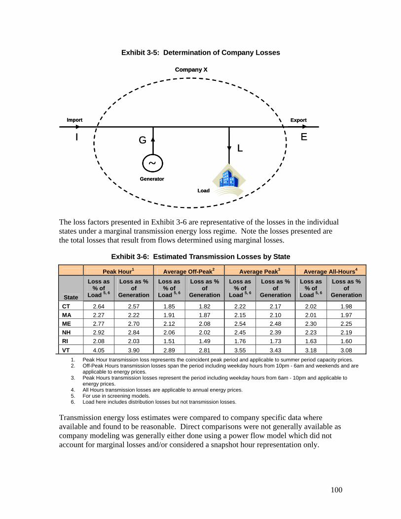
Exhibit 3-5: Determination of Company Losses
~Generator
ExportImport
Load
I EL
G
Company X
~~Generator
ExportImport
Load
I EL
G
Company X
The loss factors presented in Exhibit 3-6 are representative of the losses in the individual states under a marginal transmission energy loss regime. Note the losses presented are the total losses that result from flows determined using marginal losses.
Exhibit 3-6: Estimated Transmission Losses by State
Peak Hour1 Average Off-Peak2 Average Peak3 Average All-Hours4
State
Loss as % of
Load 5, 6
Loss as % of
Generation
Loss as % of
Load 5, 6
Loss as % of
Generation
Loss as % of
Load 5, 6
Loss as % of
Generation
Loss as % of
Load 5, 6
Loss as % of
Generation
CT 2.64 2.57 1.85 1.82 2.22 2.17 2.02 1.98 MA 2.27 2.22 1.91 1.87 2.15 2.10 2.01 1.97 ME 2.77 2.70 2.12 2.08 2.54 2.48 2.30 2.25 NH 2.92 2.84 2.06 2.02 2.45 2.39 2.23 2.19 RI 2.08 2.03 1.51 1.49 1.76 1.73 1.63 1.60 VT 4.05 3.90 2.89 2.81 3.55 3.43 3.18 3.08
1. Peak Hour transmission loss represents the coincident peak period and applicable to summer period capacity prices. 2. Off-Peak Hours transmission losses span the period including weekday hours from 10pm - 6am and weekends and are
applicable to energy prices. 3. Peak Hours transmission losses represent the period including weekday hours from 6am - 10pm and applicable to
energy prices. 4. All Hours transmission losses are applicable to annual energy prices. 5. For use in screening models. 6. Load here includes distribution losses but not transmission losses.
Transmission energy loss estimates were compared to company specific data where available and found to be reasonable. Direct comparisons were not generally available as company modeling was generally either done using a power flow model which did not account for marginal losses and/or considered a snapshot hour representation only.
100
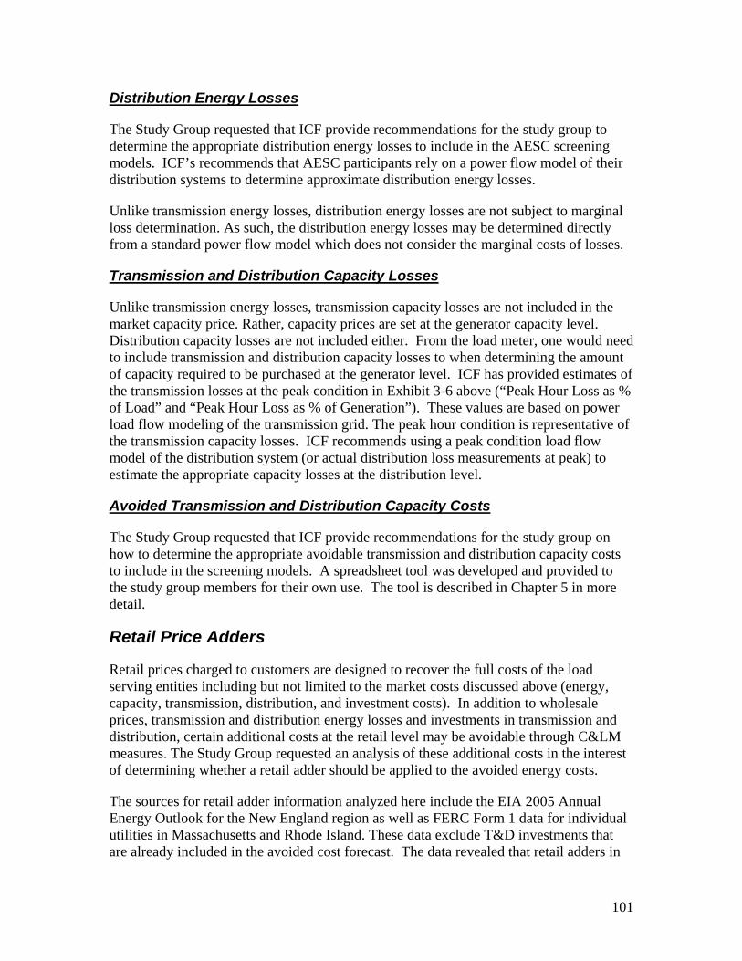
Distribution Energy Losses
The Study Group requested that ICF provide recommendations for the study group to determine the appropriate distribution energy losses to include in the AESC screening models. ICF’s recommends that AESC participants rely on a power flow model of their distribution systems to determine approximate distribution energy losses.
Unlike transmission energy losses, distribution energy losses are not subject to marginal loss determination. As such, the distribution energy losses may be determined directly from a standard power flow model which does not consider the marginal costs of losses.
Transmission and Distribution Capacity Losses
Unlike transmission energy losses, transmission capacity losses are not included in the market capacity price. Rather, capacity prices are set at the generator capacity level. Distribution capacity losses are not included either. From the load meter, one would need to include transmission and distribution capacity losses to when determining the amount of capacity required to be purchased at the generator level. ICF has provided estimates of the transmission losses at the peak condition in Exhibit 3-6 above (“Peak Hour Loss as % of Load” and “Peak Hour Loss as % of Generation”). These values are based on power load flow modeling of the transmission grid. The peak hour condition is representative of the transmission capacity losses. ICF recommends using a peak condition load flow model of the distribution system (or actual distribution loss measurements at peak) to estimate the appropriate capacity losses at the distribution level.
Avoided Transmission and Distribution Capacity Costs
The Study Group requested that ICF provide recommendations for the study group on how to determine the appropriate avoidable transmission and distribution capacity costs to include in the screening models. A spreadsheet tool was developed and provided to the study group members for their own use. The tool is described in Chapter 5 in more detail.
Retail Price Adders
Retail prices charged to customers are designed to recover the full costs of the load serving entities including but not limited to the market costs discussed above (energy, capacity, transmission, distribution, and investment costs). In addition to wholesale prices, transmission and distribution energy losses and investments in transmission and distribution, certain additional costs at the retail level may be avoidable through C&LM measures. The Study Group requested an analysis of these additional costs in the interest of determining whether a retail adder should be applied to the avoided energy costs.
The sources for retail adder information analyzed here include the EIA 2005 Annual Energy Outlook for the New England region as well as FERC Form 1 data for individual utilities in Massachusetts and Rhode Island. These data exclude T&D investments that are already included in the avoided cost forecast. The data revealed that retail adders in
101
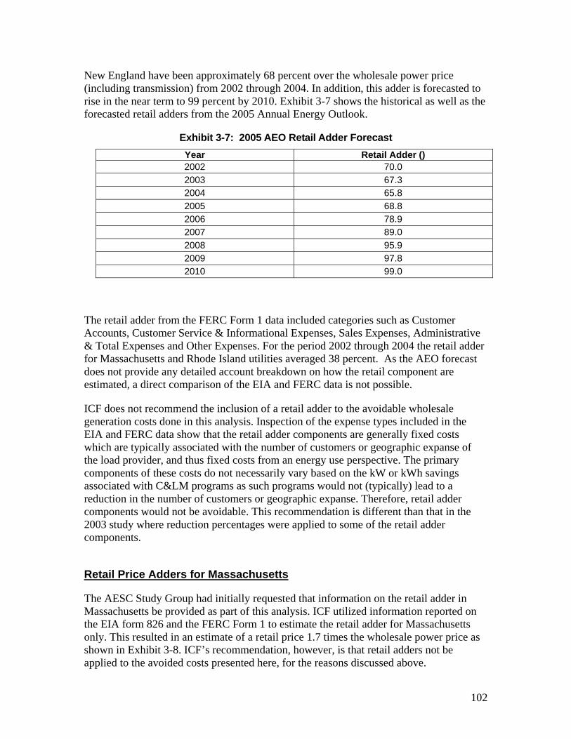
New England have been approximately 68 percent over the wholesale power price (including transmission) from 2002 through 2004. In addition, this adder is forecasted to rise in the near term to 99 percent by 2010. Exhibit 3-7 shows the historical as well as the forecasted retail adders from the 2005 Annual Energy Outlook.
Exhibit 3-7: 2005 AEO Retail Adder Forecast Year Retail Adder () 2002 70.0 2003 67.3 2004 65.8 2005 68.8 2006 78.9 2007 89.0 2008 95.9 2009 97.8 2010 99.0
The retail adder from the FERC Form 1 data included categories such as Customer Accounts, Customer Service & Informational Expenses, Sales Expenses, Administrative & Total Expenses and Other Expenses. For the period 2002 through 2004 the retail adder for Massachusetts and Rhode Island utilities averaged 38 percent. As the AEO forecast does not provide any detailed account breakdown on how the retail component are estimated, a direct comparison of the EIA and FERC data is not possible.
ICF does not recommend the inclusion of a retail adder to the avoidable wholesale generation costs done in this analysis. Inspection of the expense types included in the EIA and FERC data show that the retail adder components are generally fixed costs which are typically associated with the number of customers or geographic expanse of the load provider, and thus fixed costs from an energy use perspective. The primary components of these costs do not necessarily vary based on the kW or kWh savings associated with C&LM programs as such programs would not (typically) lead to a reduction in the number of customers or geographic expanse. Therefore, retail adder components would not be avoidable. This recommendation is different than that in the 2003 study where reduction percentages were applied to some of the retail adder components.
Retail Price Adders for Massachusetts
The AESC Study Group had initially requested that information on the retail adder in Massachusetts be provided as part of this analysis. ICF utilized information reported on the EIA form 826 and the FERC Form 1 to estimate the retail adder for Massachusetts only. This resulted in an estimate of a retail price 1.7 times the wholesale power price as shown in Exhibit 3-8. ICF’s recommendation, however, is that retail adders not be applied to the avoided costs presented here, for the reasons discussed above.
102
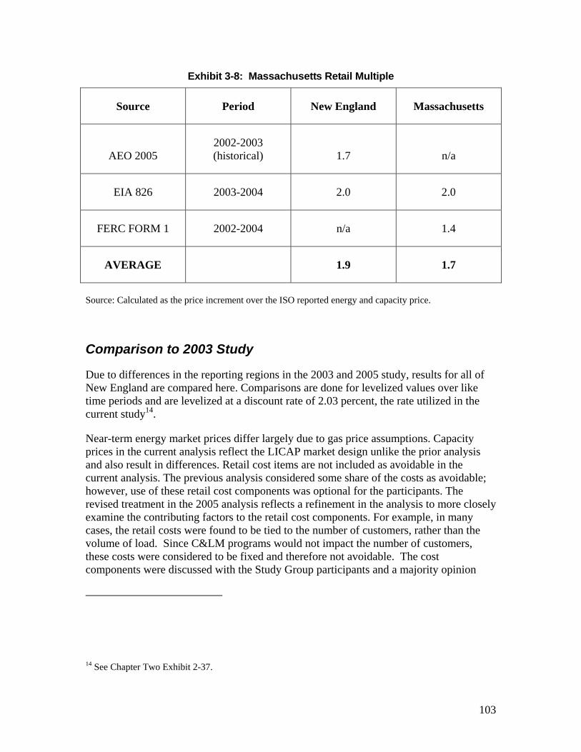
Exhibit 3-8: Massachusetts Retail Multiple
Source Period New England Massachusetts
AEO 2005 2002-2003 (historical) 1.7 n/a
EIA 826 2003-2004 2.0 2.0
FERC FORM 1 2002-2004 n/a 1.4
AVERAGE 1.9 1.7
Source: Calculated as the price increment over the ISO reported energy and capacity price.
Comparison to 2003 Study
Due to differences in the reporting regions in the 2003 and 2005 study, results for all of New England are compared here. Comparisons are done for levelized values over like time periods and are levelized at a discount rate of 2.03 percent, the rate utilized in the current study14.
Near-term energy market prices differ largely due to gas price assumptions. Capacity prices in the current analysis reflect the LICAP market design unlike the prior analysis and also result in differences. Retail cost items are not included as avoidable in the current analysis. The previous analysis considered some share of the costs as avoidable; however, use of these retail cost components was optional for the participants. The revised treatment in the 2005 analysis reflects a refinement in the analysis to more closely examine the contributing factors to the retail cost components. For example, in many cases, the retail costs were found to be tied to the number of customers, rather than the volume of load. Since C&LM programs would not impact the number of customers, these costs were considered to be fixed and therefore not avoidable. The cost components were discussed with the Study Group participants and a majority opinion
14 See Chapter Two Exhibit 2-37.
103
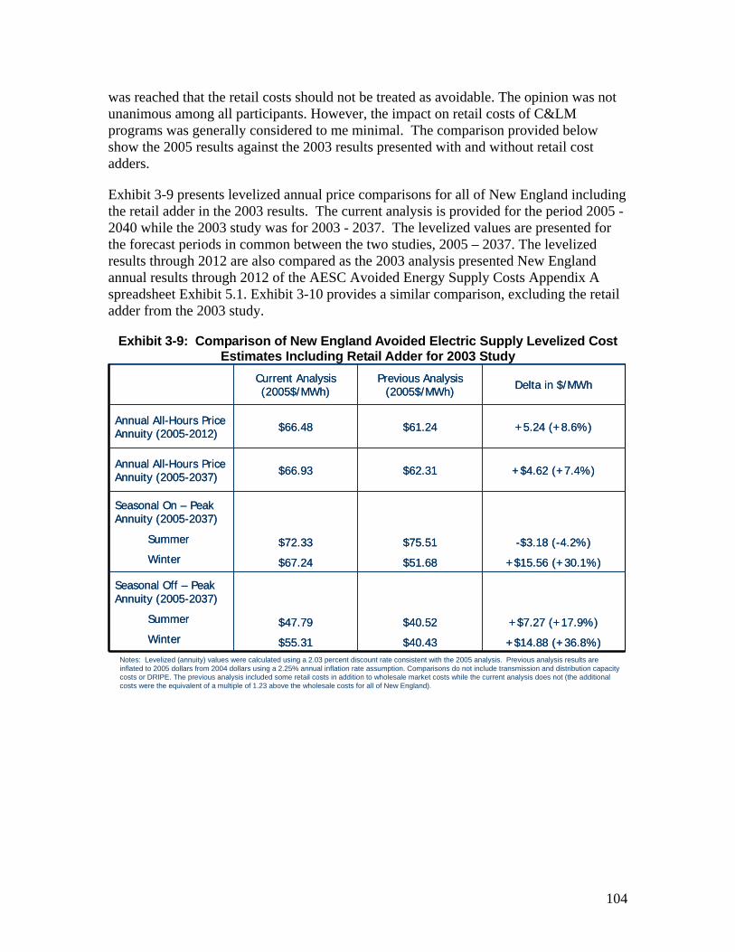
104
was reached that the retail costs should not be treated as avoidable. The opinion was not unanimous among all participants. However, the impact on retail costs of C&LM programs was generally considered to me minimal. The comparison provided below show the 2005 results against the 2003 results presented with and without retail cost adders.
Exhibit 3-9 presents levelized annual price comparisons for all of New England including the retail adder in the 2003 results. The current analysis is provided for the period 2005 -2040 while the 2003 study was for 2003 - 2037. The levelized values are presented for the forecast periods in common between the two studies, 2005 – 2037. The levelized results through 2012 are also compared as the 2003 analysis presented New England annual results through 2012 of the AESC Avoided Energy Supply Costs Appendix A spreadsheet Exhibit 5.1. Exhibit 3-10 provides a similar comparison, excluding the retail adder from the 2003 study.
Exhibit 3-9: Comparison of New England Avoided Electric Supply Levelized Cost Estimates Including Retail Adder for 2003 Study
+$4.62 (+7.4%)$62.31$66.93Annual All-Hours Price Annuity (2005-2037)
+$7.27 (+17.9%)
+$14.88 (+36.8%)
$40.52
$40.43
$47.79
$55.31
Seasonal Off – Peak Annuity (2005-2037)
Summer
Winter
-$3.18 (-4.2%)
+$15.56 (+30.1%)
$75.51
$51.68
$72.33
$67.24
Seasonal On – Peak Annuity (2005-2037)
Summer
Winter
+5.24 (+8.6%)$61.24$66.48Annual All-Hours Price Annuity (2005-2012)
Delta in $/MWhPrevious Analysis (2005$/MWh)
Current Analysis (2005$/MWh)
Notes: Levelized (annuity) values were calculated using a 2.03 percent discount rate consistent with the 2005 analysis. Previous analysis results are inflated to 2005 dollars from 2004 dollars using a 2.25% annual inflation rate assumption. Comparisons do not include transmission and distribution capacity costs or DRIPE. The previous analysis included some retail costs in addition to wholesale market costs while the current analysis does not (the additional costs were the equivalent of a multiple of 1.23 above the wholesale costs for all of New England).
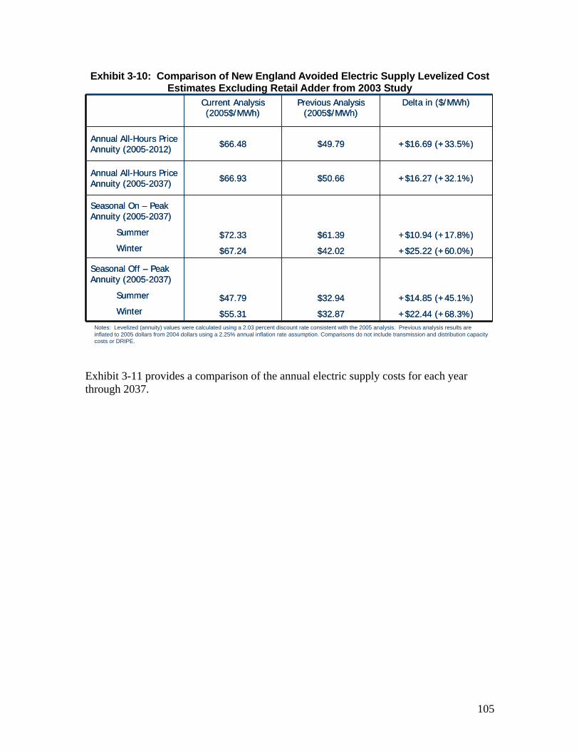
105
Exhibit 3-10: Comparison of New England Avoided Electric Supply Levelized Cost Estimates Excluding Retail Adder from 2003 Study
Exhibit 3-11 provides a comparison of the annual electric supply costs for each year through 2037.
+$16.27 (+32.1%)$50.66$66.93Annual All-Hours Price Annuity (2005-2037)
+$14.85 (+45.1%)
+$22.44 (+68.3%)
$32.94
$32.87
$47.79
$55.31
Seasonal Off – Peak Annuity (2005-2037)
Summer
Winter
+$10.94 (+17.8%)
+$25.22 (+60.0%)
$61.39
$42.02
$72.33
$67.24
Seasonal On – Peak Annuity (2005-2037)
Summer
Winter
+$16.69 (+33.5%)$49.79$66.48Annual All-Hours Price Annuity (2005-2012)
Delta in ($/MWh)Previous Analysis (2005$/MWh)
Current Analysis (2005$/MWh)
Notes: Levelized (annuity) values were calculated using a 2.03 percent discount rate consistent with the 2005 analysis. Previous analysis results are inflated to 2005 dollars from 2004 dollars using a 2.25% annual inflation rate assumption. Comparisons do not include transmission and distribution capacity costs or DRIPE.
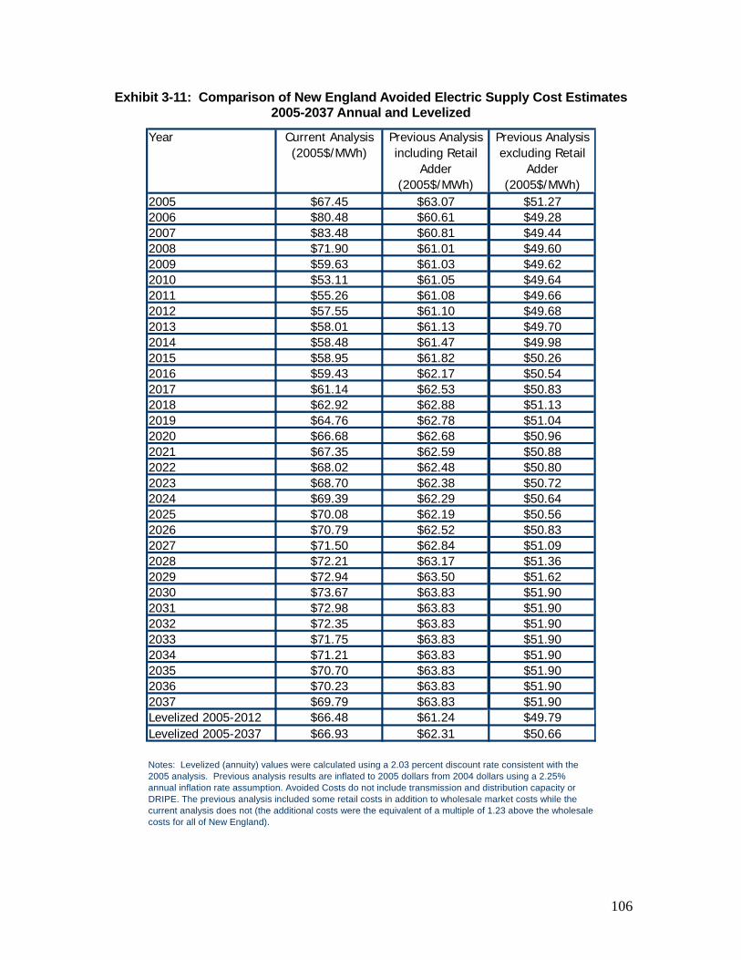
106
Exhibit 3-11: Comparison of New England Avoided Electric Supply Cost Estimates 2005-2037 Annual and Levelized
Year Current Analysis (2005$/MWh)
Previous Analysis including Retail
Adder (2005$/MWh)
Previous Analysis excluding Retail
Adder (2005$/MWh)
2005 $67.45 $63.07 $51.27 2006 $80.48 $60.61 $49.28 2007 $83.48 $60.81 $49.44 2008 $71.90 $61.01 $49.60 2009 $59.63 $61.03 $49.62 2010 $53.11 $61.05 $49.64 2011 $55.26 $61.08 $49.66 2012 $57.55 $61.10 $49.68 2013 $58.01 $61.13 $49.70 2014 $58.48 $61.47 $49.98 2015 $58.95 $61.82 $50.26 2016 $59.43 $62.17 $50.54 2017 $61.14 $62.53 $50.83 2018 $62.92 $62.88 $51.13 2019 $64.76 $62.78 $51.04 2020 $66.68 $62.68 $50.96 2021 $67.35 $62.59 $50.88 2022 $68.02 $62.48 $50.80 2023 $68.70 $62.38 $50.72 2024 $69.39 $62.29 $50.64 2025 $70.08 $62.19 $50.56 2026 $70.79 $62.52 $50.83 2027 $71.50 $62.84 $51.09 2028 $72.21 $63.17 $51.36 2029 $72.94 $63.50 $51.62 2030 $73.67 $63.83 $51.90 2031 $72.98 $63.83 $51.90 2032 $72.35 $63.83 $51.90 2033 $71.75 $63.83 $51.90 2034 $71.21 $63.83 $51.90 2035 $70.70 $63.83 $51.90 2036 $70.23 $63.83 $51.90 2037 $69.79 $63.83 $51.90 Levelized 2005-2012 $66.48 $61.24 $49.79 Levelized 2005-2037 $66.93 $62.31 $50.66
Notes: Levelized (annuity) values were calculated using a 2.03 percent discount rate consistent with the 2005 analysis. Previous analysis results are inflated to 2005 dollars from 2004 dollars using a 2.25% annual inflation rate assumption. Avoided Costs do not include transmission and distribution capacity or DRIPE. The previous analysis included some retail costs in addition to wholesale market costs while the current analysis does not (the additional costs were the equivalent of a multiple of 1.23 above the wholesale costs for all of New England).
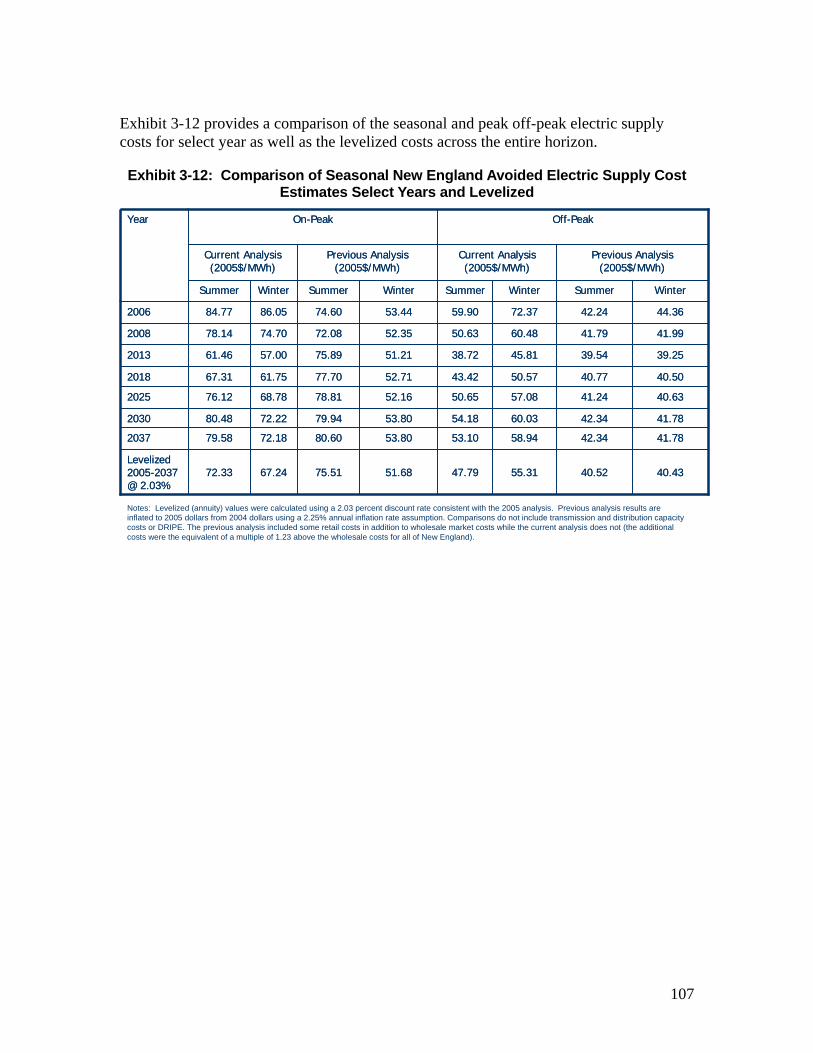
107
Exhibit 3-12 provides a comparison of the seasonal and peak off-peak electric supply costs for select year as well as the levelized costs across the entire horizon.
Exhibit 3-12: Comparison of Seasonal New England Avoided Electric Supply Cost Estimates Select Years and Levelized
40.43
41.78
41.78
40.63
40.50
39.25
41.99
44.36
Winter
40.52
42.34
42.34
41.24
40.77
39.54
41.79
42.24
Summer
Previous Analysis (2005$/MWh)
55.31
58.94
60.03
57.08
50.57
45.81
60.48
72.37
Winter
47.79
53.10
54.18
50.65
43.42
38.72
50.63
59.90
Summer
Current Analysis (2005$/MWh)
Off-PeakOn-Peak
67.24
72.18
72.22
68.78
61.75
57.00
74.70
86.05
Winter
53.8080.6079.582037
51.6875.5172.33Levelized 2005-2037 @ 2.03%
53.8079.9480.482030
52.16
52.71
51.21
52.35
53.44
WinterSummerSummer
74.6084.772006
78.8176.122025
77.7067.312018
75.8961.462013
72.0878.142008
Previous Analysis (2005$/MWh)
Current Analysis (2005$/MWh)
Year
Notes: Levelized (annuity) values were calculated using a 2.03 percent discount rate consistent with the 2005 analysis. Previous analysis results are inflated to 2005 dollars from 2004 dollars using a 2.25% annual inflation rate assumption. Comparisons do not include transmission and distribution capacity costs or DRIPE. The previous analysis included some retail costs in addition to wholesale market costs while the current analysis does not (the additional costs were the equivalent of a multiple of 1.23 above the wholesale costs for all of New England).
Chapter Four: Other Fuel Avoided Costs In this section, we describe our approach to estimating avoided costs for distillate fuel oil, residual fuel oil, kerosene, propane and wood. Our findings are shown in the exhibits below. In the following brief sections we describe our approach to estimating these avoided costs. The Energy Information Administration publication Petroleum Marketing Monthly was the source for all historical data, with the exception of data for firewood, which was obtained through calls to firewood dealers in New England and internet research. All costs are in 2005$/MMBtu.
After analyzing the impacts of Hurricane Katrina on the oil markets, we conclude that it does not warrant any change to the oil price forecast. Indeed, the situation with oil highlights the stark differences between the oil and gas market and infrastructure. The U.S. Gulf Coast and the Gulf of Mexico are vital components of the oil supply infrastructure in the United States. The hurricane initially reduced oil supplies by an estimated 1.4 million barrels per day (mmb/d). In addition, about 1.9 mmb/d of crude oil refining capacity was shut down as Katrina approached15. But oil is a global market, and this volume is still a small fraction of a large world-wide oil market of approximately 82 million barrels per day. As was demonstrated by subsequent events, the oil price spike was transitory largely because other supplies rushed in to fill the shortfall. These other supplies included releases from the Strategic Petroleum Reserve (SPR) as well as crude and product deliveries from internationals sources. As of September 13, 2005, the prices for crude oil, heating oil and residual fuel oil were near or below their levels before Hurricane Katrina hit the Gulf Coast.
Crude Oil Price Forecast
The forecasted price of all petroleum products is driven by the forecast for crude oil prices used in the gas forecast and in the power forecasts. The crude oil price used is an ICF forecast. ICF expects the crude oil prices to stay near or just below their current levels in the near term until 2010 as the supply demand situation will remain tight. Between 2010 and 2015, the prices are expected to decline as investments made in oil production capacity in the next few years will be realized in increasing oil supply. However, by 2015, the demand growth catches up with oil production capacity and the crude oil prices increases steadily for the rest of the forecast. Exhibit 4-1 graphically presents the oil price forecast.
15 Short-Term Energy Outlook, September 2005, Energy Information Administration, U.S. Department of Energy
108
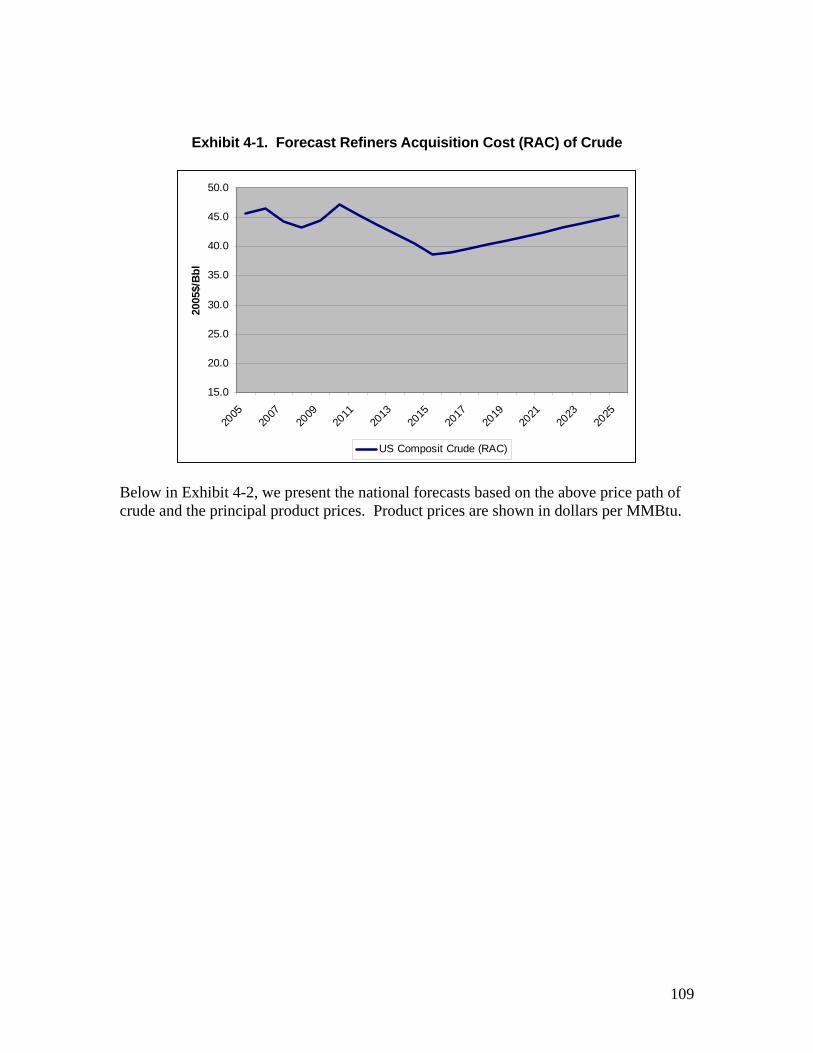
Exhibit 4-1. Forecast Refiners Acquisition Cost (RAC) of Crude
15.0
20.0
25.0
30.0
35.0
40.0
45.0
50.0
2005
2007
2009
2011
2013
2015
2017
2019
2021
2023
2025
2005
$/B
bl
US Composit Crude (RAC)
Below in Exhibit 4-2, we present the national forecasts based on the above price path of crude and the principal product prices. Product prices are shown in dollars per MMBtu.
109
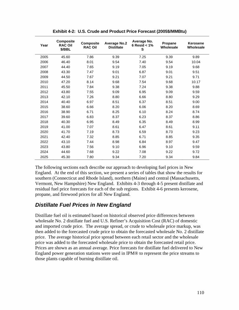
Exhibit 4-2: U.S. Crude and Product Price Forecast (2005$/MMBtu)
Year Composite
RAC Oil $/BBL
Composite RAC Oil
Average No.2 Distillate
Average No. 6 Resid < 1%
S Propane
Wholesale Kerosene Wholesale
2005 45.60 7.86 9.39 7.25 9.39 9.89 2006 46.40 8.01 9.54 7.40 9.54 10.04 2007 44.40 7.65 9.19 7.05 9.19 9.68 2008 43.30 7.47 9.01 6.87 9.01 9.51 2009 44.50 7.67 9.21 7.07 9.21 9.71 2010 47.20 8.14 9.68 7.54 9.68 10.17 2011 45.50 7.84 9.38 7.24 9.38 9.88 2012 43.80 7.55 9.09 6.95 9.09 9.59 2013 42.10 7.26 8.80 6.66 8.80 9.29 2014 40.40 6.97 8.51 6.37 8.51 9.00 2015 38.60 6.66 8.20 6.06 8.20 8.69 2016 38.90 6.71 8.25 6.10 8.24 8.74 2017 39.60 6.83 8.37 6.23 8.37 8.86 2018 40.30 6.95 8.49 6.35 8.49 8.99 2019 41.00 7.07 8.61 6.47 8.61 9.11 2020 41.70 7.19 8.73 6.59 8.73 9.23 2021 42.40 7.32 8.85 6.71 8.85 9.35 2022 43.10 7.44 8.98 6.84 8.97 9.47 2023 43.80 7.56 9.10 6.96 9.10 9.59 2024 44.60 7.68 9.22 7.08 9.22 9.72 2025 45.30 7.80 9.34 7.20 9.34 9.84
The following sections each describe our approach to developing fuel prices in New England. At the end of this section, we present a series of tables that show the results for southern (Connecticut and Rhode Island), northern (Maine) and central (Massachusetts, Vermont, New Hampshire) New England. Exhibits 4-3 through 4-5 present distillate and residual fuel price forecasts for each of the sub regions. Exhibit 4-6 presents kerosene, propane, and firewood prices for all New England.
Distillate Fuel Prices in New England
Distillate fuel oil is estimated based on historical observed price differences between wholesale No. 2 distillate fuel and U.S. Refiner’s Acquisition Cost (RAC) of domestic and imported crude price. The average spread, or crude to wholesale price markup, was then added to the forecasted crude price to obtain the forecasted wholesale No. 2 distillate price. The average historical price spread between each retail sector and the wholesale price was added to the forecasted wholesale price to obtain the forecasted retail price. Prices are shown as an annual average. Price forecasts for distillate fuel delivered to New England power generation stations were used in IPM® to represent the price streams to those plants capable of burning distillate oil.
110
New England Residual Fuel Prices: No. 6 and No. 4
Our forecast of residual fuel oil is done in the same way as the distillate forecast with the exception that retail prices were not available for individual sectors and hence a single retail price is forecasted. For No. 6 residual fuel, an average crude-to-wholesale markup, and then an average wholesale to retail markup was calculated. The No. 4 fuel oil wholesale and retail prices are simple averages of No. 2 distillate and No. 6 residual prices. IPM® models oil-fired generation and uses the appropriate fuel oil type for each unit modeled. Oil-gas steam units typically are modeled as able to utilize regional wholesale No. 6 oil and natural gas with a small markup for inter-regional transportation..
Kerosene Prices in New England
Kerosene prices are based on historical observed differences in wholesale kerosene prices with wholesale No. 2 distillate prices. The resulting forecast represents the historical average spread applied to our forecast of No. 2 distillate prices. The prices shown in Exhibit 4 -7 are for all New England. The retail price forecast was obtained in the same fashion as retail prices for distillate and residual fuel; however, the retail price represents the price to all sectors. No sector specific pricing was available.
New England Propane Pricing
We used a similar approach for propane. Distillate and propane are highly correlated; therefore we applied the average spread between historic wholesale No. 2 distillate wholesale prices and wholesale propane prices to estimate future propane prices. Retail prices were generated using the same method as the other fuels. As with kerosene, historic price data were not available on the state level but only on the regional level. Propane prices shown are thus for all New England.
Firewood in New England
Wood prices are based on data collected through calls to firewood dealers throughout the New England region and internet research. Prices were gathered for green wood, which is not ready to burn, and seasoned wood, which is ready to burn. Average prices were escalated by two percent per year in real terms. The estimated long term increase in wood pricing reflects conversations with dealers and our view of the long term growth in real gross state product (as reported by the Bureau of Economic Analysis) for New England in general. This is the same growth rate used in the previous AESC study. Prices shown are the same for all New England sub-regions.
Comparison with Previous Avoided Cost Study
As with natural gas, fuel prices have increased in all categories since the 2003 AESC study. A comparison of the fuel prices is shown below for those categories of fuel that are common to both studies. As can be seen, in many categories, levelized fuel costs have almost doubled.
111
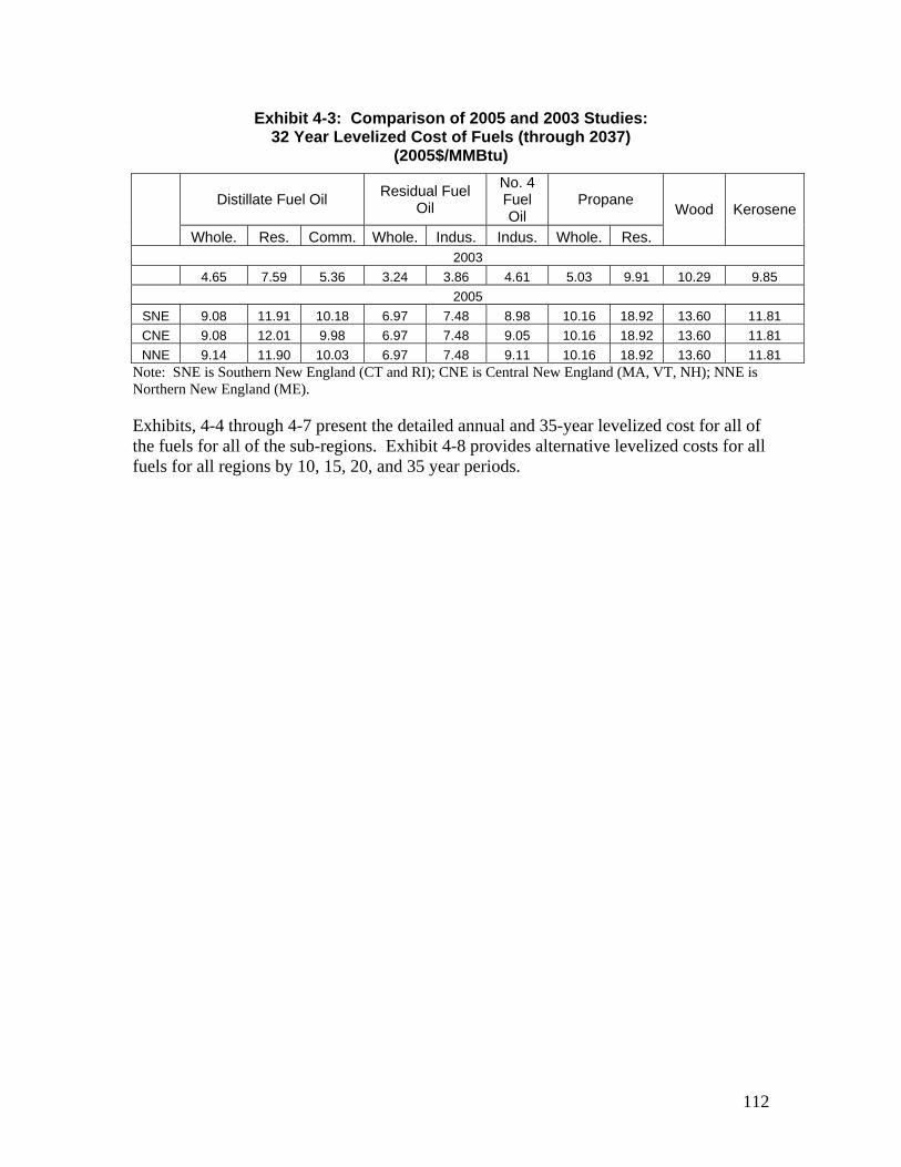
Exhibit 4-3: Comparison of 2005 and 2003 Studies: 32 Year Levelized Cost of Fuels (through 2037)
(2005$/MMBtu)
Distillate Fuel Oil Residual Fuel Oil
No. 4 Fuel Oil
Propane
Whole. Res. Comm. Whole. Indus. Indus. Whole. Res.
Wood Kerosene
2003 4.65 7.59 5.36 3.24 3.86 4.61 5.03 9.91 10.29 9.85
2005 SNE 9.08 11.91 10.18 6.97 7.48 8.98 10.16 18.92 13.60 11.81 CNE 9.08 12.01 9.98 6.97 7.48 9.05 10.16 18.92 13.60 11.81 NNE 9.14 11.90 10.03 6.97 7.48 9.11 10.16 18.92 13.60 11.81
Note: SNE is Southern New England (CT and RI); CNE is Central New England (MA, VT, NH); NNE is Northern New England (ME).
Exhibits, 4-4 through 4-7 present the detailed annual and 35-year levelized cost for all of the fuels for all of the sub-regions. Exhibit 4-8 provides alternative levelized costs for all fuels for all regions by 10, 15, 20, and 35 year periods.
112
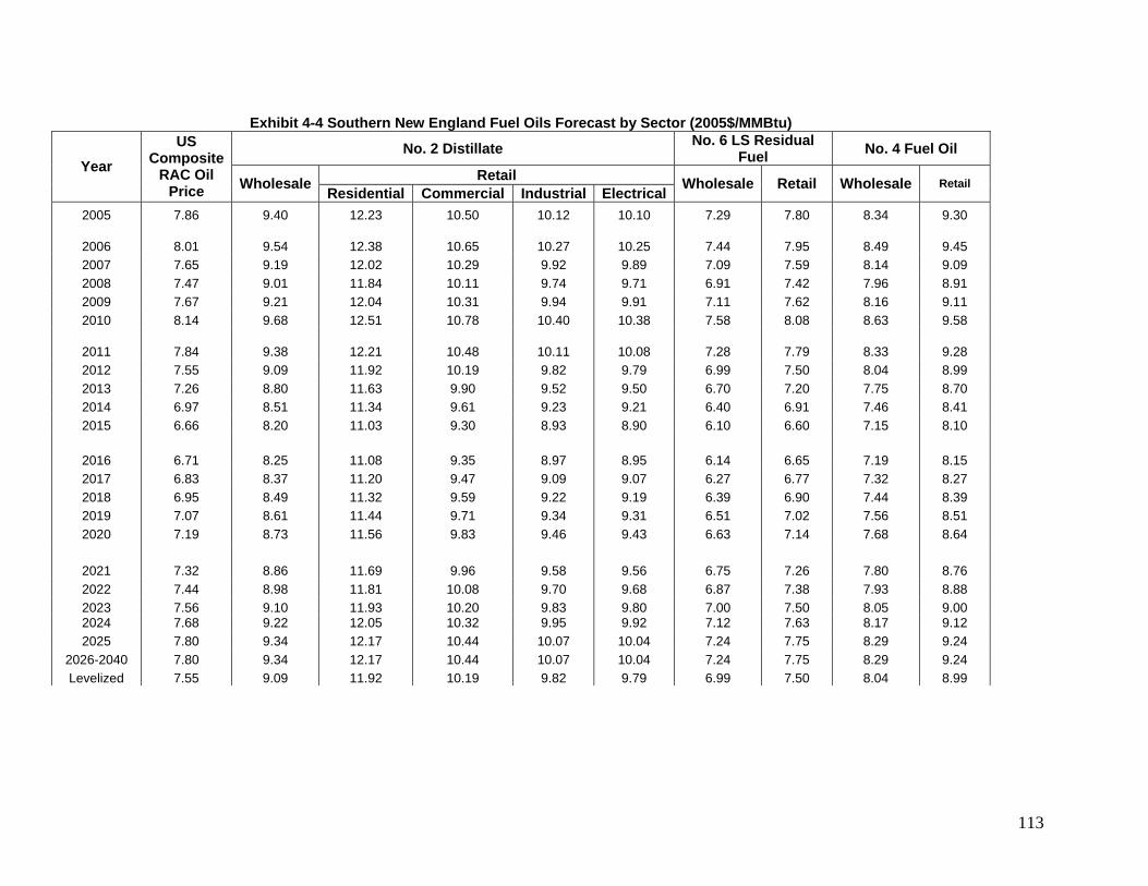
Exhibit 4-4 Southern New England Fuel Oils Forecast by Sector (2005$/MMBtu)
No. 2 Distillate No. 6 LS Residual Fuel No. 4 Fuel Oil
Retail Year US
Composite RAC Oil
Price Wholesale Residential Commercial Industrial Electrical Wholesale Retail Wholesale Retail
2005 7.86 9.40 12.23 10.50 10.12 10.10 7.29 7.80 8.34 9.30
2006 8.01 9.54 12.38 10.65 10.27 10.25 7.44 7.95 8.49 9.45 2007 7.65 9.19 12.02 10.29 9.92 9.89 7.09 7.59 8.14 9.09 2008 7.47 9.01 11.84 10.11 9.74 9.71 6.91 7.42 7.96 8.91 2009 7.67 9.21 12.04 10.31 9.94 9.91 7.11 7.62 8.16 9.11 2010 8.14 9.68 12.51 10.78 10.40 10.38 7.58 8.08 8.63 9.58
2011 7.84 9.38 12.21 10.48 10.11 10.08 7.28 7.79 8.33 9.28 2012 7.55 9.09 11.92 10.19 9.82 9.79 6.99 7.50 8.04 8.99 2013 7.26 8.80 11.63 9.90 9.52 9.50 6.70 7.20 7.75 8.70 2014 6.97 8.51 11.34 9.61 9.23 9.21 6.40 6.91 7.46 8.41 2015 6.66 8.20 11.03 9.30 8.93 8.90 6.10 6.60 7.15 8.10
2016 6.71 8.25 11.08 9.35 8.97 8.95 6.14 6.65 7.19 8.15 2017 6.83 8.37 11.20 9.47 9.09 9.07 6.27 6.77 7.32 8.27 2018 6.95 8.49 11.32 9.59 9.22 9.19 6.39 6.90 7.44 8.39 2019 7.07 8.61 11.44 9.71 9.34 9.31 6.51 7.02 7.56 8.51 2020 7.19 8.73 11.56 9.83 9.46 9.43 6.63 7.14 7.68 8.64
2021 7.32 8.86 11.69 9.96 9.58 9.56 6.75 7.26 7.80 8.76 2022 7.44 8.98 11.81 10.08 9.70 9.68 6.87 7.38 7.93 8.88 2023 7.56 9.10 11.93 10.20 9.83 9.80 7.00 7.50 8.05 9.00 2024 7.68 9.22 12.05 10.32 9.95 9.92 7.12 7.63 8.17 9.12 2025 7.80 9.34 12.17 10.44 10.07 10.04 7.24 7.75 8.29 9.24
2026-2040 7.80 9.34 12.17 10.44 10.07 10.04 7.24 7.75 8.29 9.24 Levelized 7.55 9.09 11.92 10.19 9.82 9.79 6.99 7.50 8.04 8.99
113
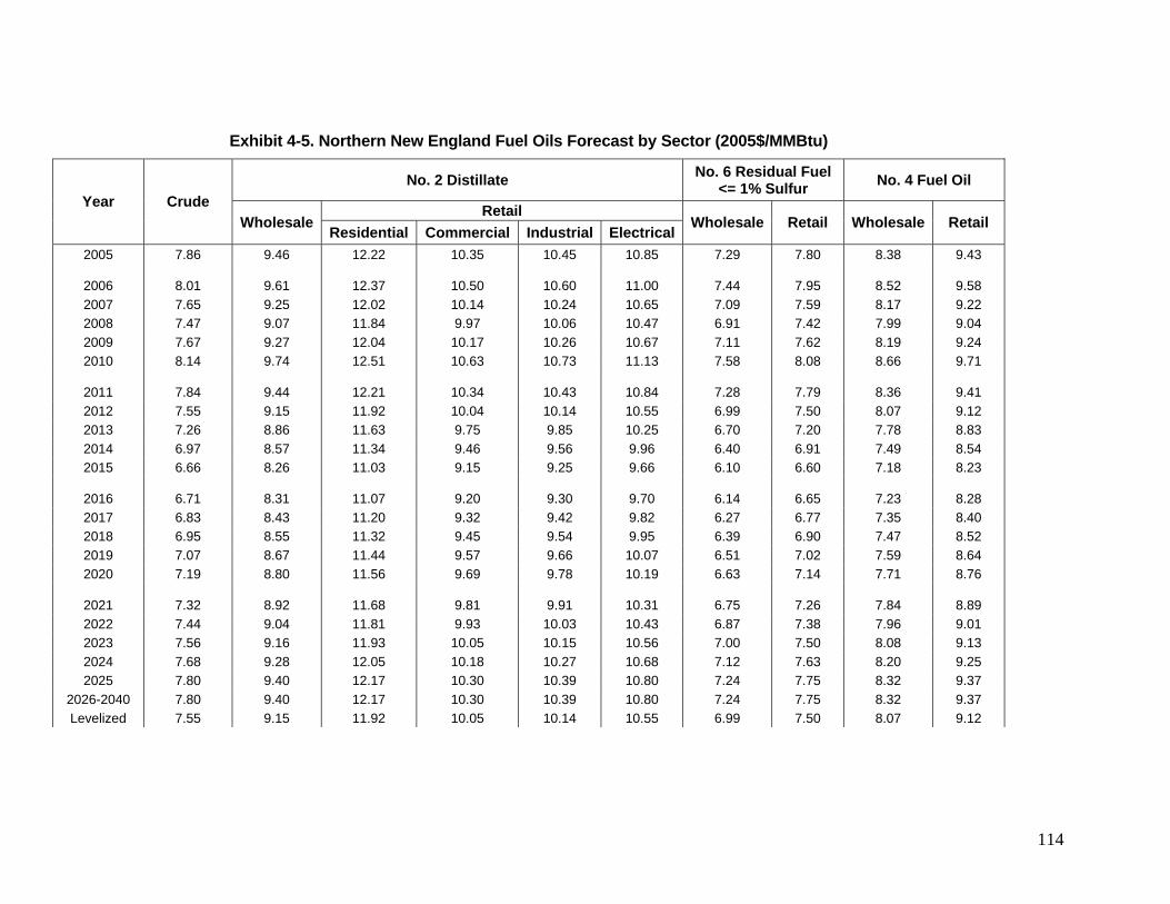
Exhibit 4-5. Northern New England Fuel Oils Forecast by Sector (2005$/MMBtu)
No. 2 Distillate No. 6 Residual Fuel <= 1% Sulfur No. 4 Fuel Oil
Retail Year Crude Wholesale Residential Commercial Industrial Electrical Wholesale Retail Wholesale Retail
2005 7.86 9.46 12.22 10.35 10.45 10.85 7.29 7.80 8.38 9.43
2006 8.01 9.61 12.37 10.50 10.60 11.00 7.44 7.95 8.52 9.58 2007 7.65 9.25 12.02 10.14 10.24 10.65 7.09 7.59 8.17 9.22 2008 7.47 9.07 11.84 9.97 10.06 10.47 6.91 7.42 7.99 9.04 2009 7.67 9.27 12.04 10.17 10.26 10.67 7.11 7.62 8.19 9.24 2010 8.14 9.74 12.51 10.63 10.73 11.13 7.58 8.08 8.66 9.71
2011 7.84 9.44 12.21 10.34 10.43 10.84 7.28 7.79 8.36 9.41 2012 7.55 9.15 11.92 10.04 10.14 10.55 6.99 7.50 8.07 9.12 2013 7.26 8.86 11.63 9.75 9.85 10.25 6.70 7.20 7.78 8.83 2014 6.97 8.57 11.34 9.46 9.56 9.96 6.40 6.91 7.49 8.54 2015 6.66 8.26 11.03 9.15 9.25 9.66 6.10 6.60 7.18 8.23
2016 6.71 8.31 11.07 9.20 9.30 9.70 6.14 6.65 7.23 8.28 2017 6.83 8.43 11.20 9.32 9.42 9.82 6.27 6.77 7.35 8.40 2018 6.95 8.55 11.32 9.45 9.54 9.95 6.39 6.90 7.47 8.52 2019 7.07 8.67 11.44 9.57 9.66 10.07 6.51 7.02 7.59 8.64 2020 7.19 8.80 11.56 9.69 9.78 10.19 6.63 7.14 7.71 8.76
2021 7.32 8.92 11.68 9.81 9.91 10.31 6.75 7.26 7.84 8.89 2022 7.44 9.04 11.81 9.93 10.03 10.43 6.87 7.38 7.96 9.01 2023 7.56 9.16 11.93 10.05 10.15 10.56 7.00 7.50 8.08 9.13 2024 7.68 9.28 12.05 10.18 10.27 10.68 7.12 7.63 8.20 9.25 2025 7.80 9.40 12.17 10.30 10.39 10.80 7.24 7.75 8.32 9.37
2026-2040 7.80 9.40 12.17 10.30 10.39 10.80 7.24 7.75 8.32 9.37 Levelized 7.55 9.15 11.92 10.05 10.14 10.55 6.99 7.50 8.07 9.12
114
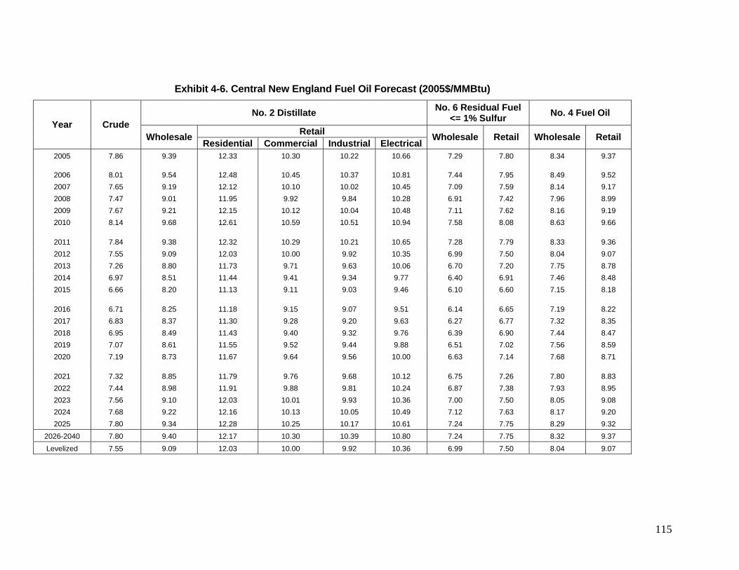
Exhibit 4-6. Central New England Fuel Oil Forecast (2005$/MMBtu)
No. 2 Distillate No. 6 Residual Fuel <= 1% Sulfur No. 4 Fuel Oil
Retail Year Crude
Wholesale Residential Commercial Industrial Electrical Wholesale Retail Wholesale Retail
2005 7.86 9.39 12.33 10.30 10.22 10.66 7.29 7.80 8.34 9.37
2006 8.01 9.54 12.48 10.45 10.37 10.81 7.44 7.95 8.49 9.52 2007 7.65 9.19 12.12 10.10 10.02 10.45 7.09 7.59 8.14 9.17 2008 7.47 9.01 11.95 9.92 9.84 10.28 6.91 7.42 7.96 8.99 2009 7.67 9.21 12.15 10.12 10.04 10.48 7.11 7.62 8.16 9.19 2010 8.14 9.68 12.61 10.59 10.51 10.94 7.58 8.08 8.63 9.66
2011 7.84 9.38 12.32 10.29 10.21 10.65 7.28 7.79 8.33 9.36 2012 7.55 9.09 12.03 10.00 9.92 10.35 6.99 7.50 8.04 9.07 2013 7.26 8.80 11.73 9.71 9.63 10.06 6.70 7.20 7.75 8.78 2014 6.97 8.51 11.44 9.41 9.34 9.77 6.40 6.91 7.46 8.48 2015 6.66 8.20 11.13 9.11 9.03 9.46 6.10 6.60 7.15 8.18
2016 6.71 8.25 11.18 9.15 9.07 9.51 6.14 6.65 7.19 8.22 2017 6.83 8.37 11.30 9.28 9.20 9.63 6.27 6.77 7.32 8.35 2018 6.95 8.49 11.43 9.40 9.32 9.76 6.39 6.90 7.44 8.47 2019 7.07 8.61 11.55 9.52 9.44 9.88 6.51 7.02 7.56 8.59 2020 7.19 8.73 11.67 9.64 9.56 10.00 6.63 7.14 7.68 8.71
2021 7.32 8.85 11.79 9.76 9.68 10.12 6.75 7.26 7.80 8.83 2022 7.44 8.98 11.91 9.88 9.81 10.24 6.87 7.38 7.93 8.95 2023 7.56 9.10 12.03 10.01 9.93 10.36 7.00 7.50 8.05 9.08 2024 7.68 9.22 12.16 10.13 10.05 10.49 7.12 7.63 8.17 9.20 2025 7.80 9.34 12.28 10.25 10.17 10.61 7.24 7.75 8.29 9.32
2026-2040 7.80 9.40 12.17 10.30 10.39 10.80 7.24 7.75 8.32 9.37 Levelized 7.55 9.09 12.03 10.00 9.92 10.36 6.99 7.50 8.04 9.07
115

Exhibit 4-7. All New England Other Fuels Forecast (2005$/MMBtu)
Propane Kerosene Wood Retail Retail Retail Year
Wholesale Residential Commercial Industrial Wholesale Retail Greenwood Seasoned 2005 10.48 19.24 15.28 13.29 9.61 12.32 8.04 10.54
2006 10.63 19.39 15.43 13.44 9.57 12.27 8.21 10.75 2007 10.28 19.04 15.08 13.09 9.21 11.92 8.37 10.97 2008 10.10 18.86 14.90 12.91 9.03 11.74 8.54 11.19 2009 10.30 19.06 15.10 13.11 9.23 11.94 8.71 11.41 2010 10.76 19.52 15.57 13.58 9.70 12.41 8.88 11.64
2011 10.47 19.23 15.27 13.28 9.40 12.11 9.06 11.87 2012 10.18 18.94 14.98 12.99 9.11 11.82 9.24 12.11 2013 9.88 18.64 14.69 12.70 8.82 11.53 9.43 12.35 2014 9.59 18.35 14.40 12.41 8.53 11.24 9.61 12.60 2015 9.29 18.05 14.09 12.10 8.22 10.93 9.81 12.85
2016 9.33 18.09 14.14 12.15 8.27 10.97 10.00 13.11 2017 9.45 18.21 14.26 12.27 8.39 11.10 10.20 13.37 2018 9.58 18.34 14.38 12.39 8.51 11.22 10.41 13.64 2019 9.70 18.46 14.50 12.51 8.63 11.34 10.61 13.91 2020 9.82 18.58 14.62 12.63 8.75 11.46 10.83 14.19
2021 9.94 18.70 14.74 12.75 8.88 11.58 11.04 14.47 2022 10.06 18.82 14.87 12.88 9.00 11.71 11.26 14.76 2023 10.18 18.95 14.99 13.00 9.12 11.83 11.49 15.06 2024 10.31 19.07 15.11 13.12 9.24 11.95 11.72 15.36 2025 10.43 19.19 15.23 13.24 9.36 12.07 11.95 15.66 2026-2040 10.43 19.19 15.23 13.24 9.36 12.07 11.95 15.66
Levelized 10.18 18.94 14.98 12.99 9.12 11.83 10.47 13.72
116
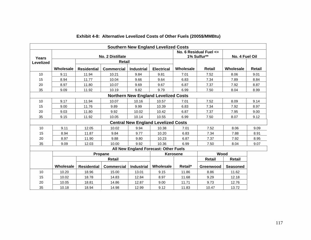
Exhibit 4-8: Alternative Levelized Costs of Other Fuels (2005$/MMBtu)
Southern New England Levelized Costs
No. 2 Distillate No. 6 Residual Fuel <=
1% Sulfur** No. 4 Fuel Oil Retail
Years Levelized
Wholesale Residential Commercial Industrial Electrical Wholesale Retail Wholesale Retail 10 9.11 11.94 10.21 9.84 9.81 7.01 7.52 8.06 9.01 15 8.94 11.77 10.04 9.66 9.64 6.83 7.34 7.89 8.84 20 8.97 11.80 10.07 9.69 9.67 6.87 7.37 7.92 8.87 35 9.09 11.92 10.19 9.82 9.79 6.99 7.50 8.04 8.99
Northern New England Levelized Costs 10 9.17 11.94 10.07 10.16 10.57 7.01 7.52 8.09 9.14 15 9.00 11.76 9.89 9.99 10.39 6.83 7.34 7.92 8.97 20 9.03 11.80 9.92 10.02 10.42 6.87 7.37 7.95 9.00 35 9.15 11.92 10.05 10.14 10.55 6.99 7.50 8.07 9.12
Central New England Levelized Costs 10 9.11 12.05 10.02 9.94 10.38 7.01 7.52 8.06 9.09 15 8.94 11.87 9.84 9.77 10.20 6.83 7.34 7.88 8.91 20 8.97 11.90 9.88 9.80 10.23 6.87 7.37 7.92 8.95 35 9.09 12.03 10.00 9.92 10.36 6.99 7.50 8.04 9.07
All New England Forecast: Other Fuels Propane Kerosene Wood
Retail Retail Retail Wholesale Residential Commercial Industrial Wholesale Retail* Greenwood Seasoned
10 10.20 18.96 15.00 13.01 9.15 11.86 8.86 11.62 15 10.02 18.78 14.83 12.84 8.97 11.68 9.29 12.18 20 10.05 18.81 14.86 12.87 9.00 11.71 9.73 12.76 35 10.18 18.94 14.98 12.99 9.12 11.83 10.47 13.72
117
118
Chapter Five: Avoided Transmission and Distribution Capacity Costs For the avoided energy supply cost analysis, ICF has recommended a methodological approach to determining avoided capacity costs for transmission and distribution and has provided a spreadsheet (Microsoft Excel) tool to allow individual Study Group members to implement the approach. The intent of this part of the analysis was to provide a common approach that could be adopted by all members of the Study Group in order to establish a consistent and defendable approach. The spreadsheet tool was provided to members of the AESC Study Group over the course of this analysis to allow for each company to enter company-specific data.
The initial step of this task was a data collection effort that ICF undertook to understand the approaches currently being used by the AESC Study Group members. After discussions and data exchange with several of the Study Group participants including National Grid, United Illuminating, NStar, and Unitil regarding their current methodology for determining avoided transmission and distribution capacity costs, it was apparent that a variety of approaches were used. However, in a number of cases, the results approximated the average system cost, rather than the incremental or avoidable costs (by dividing annual revenue requirements for T&D operations by the average annual peak over a historical period).
It was also apparent that the availability and quality of data necessary to develop reasonable estimates of marginal T&D costs varied from company to company. In order to accommodate this, ICF attempted to develop a methodology that largely relies on data which should be common to all companies in developing the tool, yet be flexible enough to utilize custom inputs that may be available at individual companies. Our method should produce a reasonable proxy for the marginal costs of such services.
This remainder of this chapter presents the approach and provides an overview of the tool. Note, all exhibits shown in this chapter are intended to be illustrative only and should not be relied on by any company.
Summary of Transmission and Distribution Avoided Capacity Cost Calculator
The transmission and distribution avoided cost calculator is comprised of four main schedules and one appendix schedule on which users provide critical inputs to feed the avoided cost calculation. The tool is created in Microsoft Excel, which was noted to be readily available to all participants. This Excel workbook allows participants to calculate their marginal costs by cataloging investments and expenses and peak demand growth over historical and forecast periods. The schedules contained in the workbook are
1. A summary schedule detailing the transmission and distribution avoided capacity costs resulting from the analysis
2. A schedule cataloging investments in T&D systems over a period of years
3. A schedule calculating the annual carrying charge of those investments based on
119
assumptions on taxes, financing costs, operational expenses, and other recurring costs.
4. A schedule cataloging peak demand growth over the same period of years
So long as participants have available to them the information needed to calculate marginal costs for the system (or are able to make reasonable assumptions for missing data elements) this proposal offers a way to calculate marginal costs appropriate to each participant’s system. Much the required data is available directly from FERC Form 1. However, some data from the FERC Form 1 may need to be interpreted or adjusted to a definition consistent with the methodology. For example, a user must estimate directly the amount of transmission and distribution investment corresponding directly to load growth, a value not directly available from the FERC Form 1.
A description of each schedule is provided below.
Schedule 1 - Summary
Schedule 1 of the tool presents the results of the avoided cost calculation for both transmission and distribution capacity. The avoided costs in $ per kilowatt-year are here defined as the incremental investment that occurs over a period of time that can be attributed to load growth divided by the actual load growth in that period. This approach reflects a reasonable proxy for the incremental costs of investment associated with transmission and distribution. Schedule 1 is illustrated in Exhibit 5-1.
The time period over which data are available for and the quality of those data are very important to this calculation. ICF recommends that a 25 period be used (15 historical and 10 forecast) given the lumpiness in the transmission investment cycle. Since the amount and quality of data does vary, users of the tool can determine the number of years to be included in the analysis (noted in later schedules) and can enter the relative importance with which they would like the historical data be given in the cost determination versus that given to the forecast data. In Schedule 1, the single user input is an indication of the weighing that users would like to give to the historical and forecast data. For example, if a user believes the historical data to be faulty, yet reflective of the trend in investment costs, but believes the forecast data is of a higher quality, that user would weight the forecast data at a higher value than the historical data. The user provides his preferred weighting as a percent for the historical data in row 5 and the weighting for the forecast data will be determined as the difference to reach 100 percent total. The resulting weighted values for transmission and distribution avoided capacity costs are found in rows 6 and 6a respectively under the column heading “Avoided Capacity Costs – Weighted”. Alternatively, if the user prefers to have no distinction in the forecast and historical series such that they would combine to be treated as one continuous time period, the values presented in the column titled “Avoided Capacity Costs – No Weighting” should be used.
Instructions for this schedule are provided in the “Source” column on the far right and possible errors will appear to the bottom of the sheet.
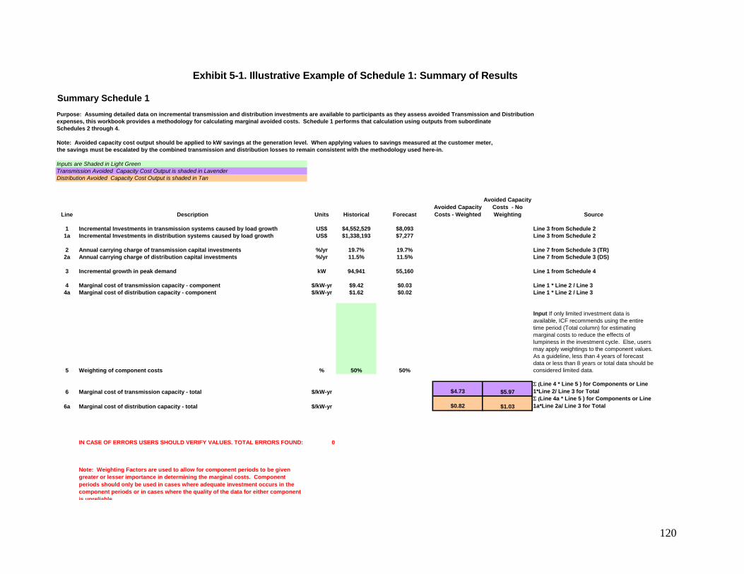
120
Exhibit 5-1. Illustrative Example of Schedule 1: Summary of Results
Summary Schedule 1Purpose: Assuming detailed data on incremental transmission and distribution investments are available to participants as they assess avoided Transmission and Distributionexpenses, this workbook provides a methodology for calculating marginal avoided costs. Schedule 1 performs that calculation using outputs from subordinate Schedules 2 through 4.
Note: Avoided capacity cost output should be applied to kW savings at the generation level. When applying values to savings measured at the customer meter, the savings must be escalated by the combined transmission and distribution losses to remain consistent with the methodology used here-in.
Inputs are Shaded in Light GreenTransmission Avoided Capacity Cost Output is shaded in LavenderDistribution Avoided Capacity Cost Output is shaded in Tan
Line Description Units Historical ForecastAvoided Capacity Costs - Weighted
Avoided Capacity Costs - No Weighting Source
1 Incremental Investments in transmission systems caused by load growth US$ $4,552,529 $8,093 Line 3 from Schedule 21a Incremental Investments in distribution systems caused by load growth US$ $1,338,193 $7,277 Line 3 from Schedule 2
2 Annual carrying charge of transmission capital investments %/yr 19.7% 19.7% Line 7 from Schedule 3 (TR)2a Annual carrying charge of distribution capital investments %/yr 11.5% 11.5% Line 7 from Schedule 3 (DS)
3 Incremental growth in peak demand kW 94,941 55,160 Line 1 from Schedule 4
4 Marginal cost of transmission capacity - component $/kW-yr $9.42 $0.03 Line 1 * Line 2 / Line 34a Marginal cost of distribution capacity - component $/kW-yr $1.62 $0.02 Line 1 * Line 2 / Line 3
5 Weighting of component costs % 50% 50%
Input If only limited investment data is available, ICF recommends using the entire time period (Total column) for estimating marginal costs to reduce the effects of lumpiness in the investment cycle. Else, users may apply weightings to the component values. As a guideline, less than 4 years of forecast data or less than 8 years or total data should be considered limited data.
6 Marginal cost of transmission capacity - total $/kW-yr $4.73 $5.97Σ (Line 4 * Line 5 ) for Components or Line 1*Line 2/ Line 3 for Total
6a Marginal cost of distribution capacity - total $/kW-yr $0.82 $1.03Σ (Line 4a * Line 5 ) for Components or Line 1a*Line 2a/ Line 3 for Total
0 0
0 0
0 0
IN CASE OF ERRORS USERS SHOULD VERIFY VALUES. TOTAL ERRORS FOUND: 0
Note: Weighting Factors are used to allow for component periods to be given greater or lesser importance in determining the marginal costs. Component periods should only be used in cases where adequate investment occurs in the component periods or in cases where the quality of the data for either component is unreliable.
121
Schedule 2 - Transmission and Distribution Investment
Schedule 2 allows users to enter capital investments made on transmission and distribution systems over a specific historical and/or future time period. The time period requires a duration over which a reasonable amount of investment occurred or is projected to occur; recommended is 25 years in length - 15 historical years and 10 forecast years.
The data on investment costs should be entered in the amount that was or is expected to be spent in each year in nominal dollars. These data are summed to determine the incremental investment which has occurred over the base year to the final year in the series. Users also specify the share (in a percentage) of the total investment which is believed to be related to load growth. The default for this is set to 50 percent of the transmission and distribution investment. This estimate was provided by one of the study participants and accepted by the Study Group as the default level.
The data are entered in nominal dollars but are converted to real dollars using the Handy-Whitman index for utility transmission and distribution costs trends for a long-term historical period. Transmission investment costs have increased at a rate above general inflation which is reflected in the Handy-Whitman derived escalation factor. Note, the historical relationship of transmission costs to general inflation is assumed to continue at the historical rate going forward.
The “Source” column provides an explanation of the calculations or instruction on the data input.
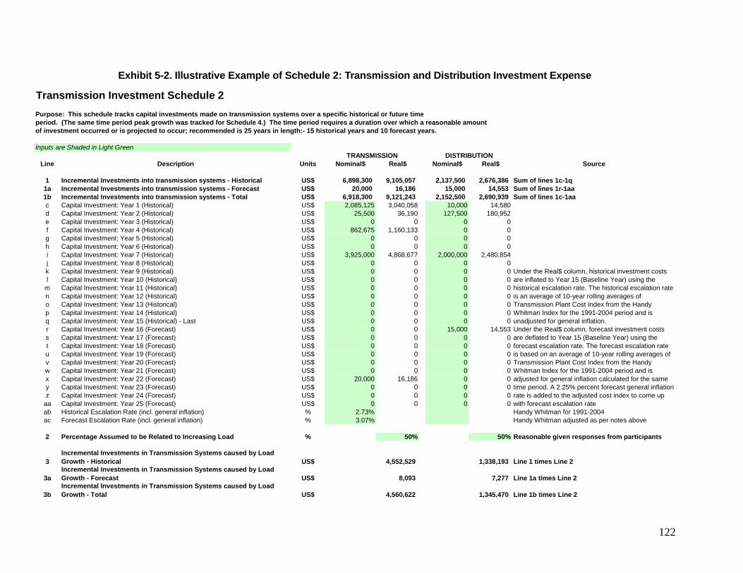
122
Exhibit 5-2. Illustrative Example of Schedule 2: Transmission and Distribution Investment Expense
Transmission Investment Schedule 2Purpose: This schedule tracks capital investments made on transmission systems over a specific historical or future time period. (The same time period peak growth was tracked for Schedule 4.) The time period requires a duration over which a reasonable amount of investment occurred or is projected to occur; recommended is 25 years in length:- 15 historical years and 10 forecast years.
Inputs are Shaded in Light GreenTRANSMISSION DISTRIBUTION
Line Description Units Nominal$ Real$ Nominal$ Real$ Source
1 Incremental Investments into transmission systems - Historical US$ 6,898,300 9,105,057 2,137,500 2,676,386 Sum of lines 1c-1q1a Incremental Investments into transmission systems - Forecast US$ 20,000 16,186 15,000 14,553 Sum of lines 1r-1aa1b Incremental Investments into transmission systems - Total US$ 6,918,300 9,121,243 2,152,500 2,690,939 Sum of lines 1c-1aac Capital Investment: Year 1 (Historical) US$ 2,085,125 3,040,058 10,000 14,580d Capital Investment: Year 2 (Historical) US$ 25,500 36,190 127,500 180,952e Capital Investment: Year 3 (Historical) US$ 0 0 0 0f Capital Investment: Year 4 (Historical) US$ 862,675 1,160,133 0 0g Capital Investment: Year 5 (Historical) US$ 0 0 0 0h Capital Investment: Year 6 (Historical) US$ 0 0 0 0i Capital Investment: Year 7 (Historical) US$ 3,925,000 4,868,677 2,000,000 2,480,854j Capital Investment: Year 8 (Historical) US$ 0 0 0 0k Capital Investment: Year 9 (Historical) US$ 0 0 0 0l Capital Investment: Year 10 (Historical) US$ 0 0 0 0
m Capital Investment: Year 11 (Historical) US$ 0 0 0 0n Capital Investment: Year 12 (Historical) US$ 0 0 0 0o Capital Investment: Year 13 (Historical) US$ 0 0 0 0p Capital Investment: Year 14 (Historical) US$ 0 0 0 0q Capital Investment: Year 15 (Historical) - Last US$ 0 0 0 0r Capital Investment: Year 16 (Forecast) US$ 0 0 15,000 14,553s Capital Investment: Year 17 (Forecast) US$ 0 0 0 0t Capital Investment: Year 18 (Forecast) US$ 0 0 0 0u Capital Investment: Year 19 (Forecast) US$ 0 0 0 0v Capital Investment: Year 20 (Forecast) US$ 0 0 0 0w Capital Investment: Year 21 (Forecast) US$ 0 0 0 0x Capital Investment: Year 22 (Forecast) US$ 20,000 16,186 0 0y Capital Investment: Year 23 (Forecast) US$ 0 0 0 0z Capital Investment: Year 24 (Forecast) US$ 0 0 0 0
aa Capital Investment: Year 25 (Forecast) US$ 0 0 0 0ab Historical Escalation Rate (incl. general inflation) % 2.73% Handy Whitman for 1991-2004ac Forecast Escalation Rate (incl. general inflation) % 3.07% Handy Whitman adjusted as per notes above
2 Percentage Assumed to be Related to Increasing Load % 50% 50% Reasonable given responses from participants
3Incremental Investments in Transmission Systems caused by Load Growth - Historical US$ 4,552,529 1,338,193 Line 1 times Line 2
3aIncremental Investments in Transmission Systems caused by Load Growth - Forecast US$ 8,093 7,277 Line 1a times Line 2
3bIncremental Investments in Transmission Systems caused by Load Growth - Total US$ 4,560,622 1,345,470 Line 1b times Line 2
Under the Real$ column, historical investment costs are inflated to Year 15 (Baseline Year) using the historical escalation rate. The historical escalation rate is an average of 10-year rolling averages of Transmission Plant Cost Index from the Handy Whitman Index for the 1991-2004 period and is unadjusted for general inflation.Under the Real$ column, forecast investment costs are deflated to Year 15 (Baseline Year) using the forecast escalation rate. The forecast escalation rate is based on an average of 10-year rolling averages of Transmission Plant Cost Index from the Handy Whitman Index for the 1991-2004 period and is adjusted for general inflation calculated for the same time period. A 2.25% percent forecast general inflation rate is added to the adjusted cost index to come up with forecast escalation rate

123
Schedule 3 – Carrying Charge Rate
Separate worksheets are provided to calculate the carrying charges for transmission and distribution capacity. The carrying charge includes insurance, taxes, depreciation, interest, and operations and maintenance.
The values input by users for each of these line items should reflect the costs associated with new investment which can be avoided. In several cases such as insurance and property tax expense, the full value associated with that item would be avoidable and it is appropriate to apply the share of the costs associated with that line item calculated as a percent of the total existing costs as the avoidable amount However, in the case of operations and maintenance cost, new investment projects benefit substantially through economies of scale gained from existing investment. Given these economies, the O&M for new investments would be a much smaller share of the total project costs than the existing O&M expenses are of the current existing plant. To allow users to better define the avoidable O&M expenses, a separate calculation for O&M inputs to the carrying charge rate calculation is provided in Appendix 1 as discussed below.
The standard data for the carrying charge calculation largely rely on FERC Form 1 as shown in the “Source” column. The formulas for each of the line items are shown in the “Source / Notes” column to the right of the schedule.
As with all other inputs in this spreadsheet, the carrying charge is required to be in real dollars. Values entered in nominal dollars will be converted to real dollars using the inflation rate input in row 8. The default annual inflation rate is set at 2.25 percent, roughly consistent with the historical long-term inflation rate and used elsewhere in the study.
Exhibit 5-3 below provides an illustrative example of the carrying charge calculation for transmission capacity. A schedule for distribution capacity having identical formulation and format is included in the tool though it is not shown here.
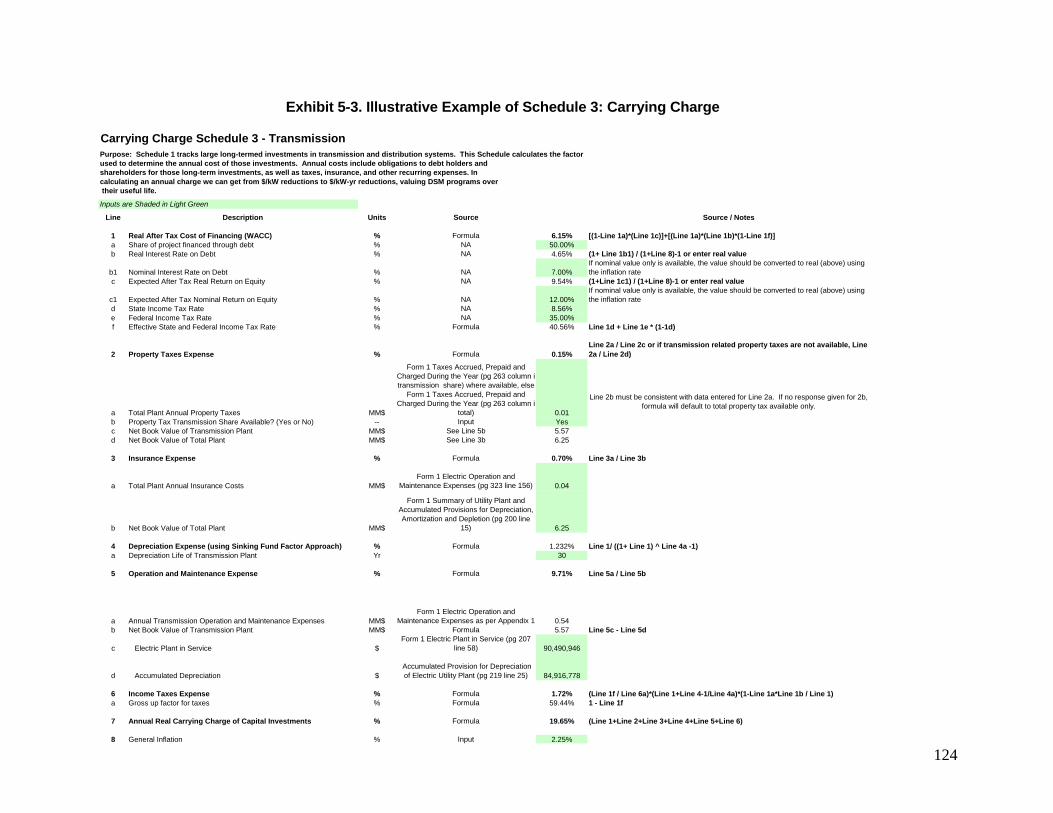
124
Exhibit 5-3. Illustrative Example of Schedule 3: Carrying Charge
Carrying Charge Schedule 3 - TransmissionPurpose: Schedule 1 tracks large long-termed investments in transmission and distribution systems. This Schedule calculates the factor used to determine the annual cost of those investments. Annual costs include obligations to debt holders and shareholders for those long-term investments, as well as taxes, insurance, and other recurring expenses. In calculating an annual charge we can get from $/kW reductions to $/kW-yr reductions, valuing DSM programs over their useful life.
Inputs are Shaded in Light Green
Line Description Units Source Source / Notes
1 Real After Tax Cost of Financing (WACC) % Formula 6.15% [(1-Line 1a)*(Line 1c)]+[(Line 1a)*(Line 1b)*(1-Line 1f)]a Share of project financed through debt % NA 50.00%b Real Interest Rate on Debt % NA 4.65% (1+ Line 1b1) / (1+Line 8)-1 or enter real value
b1 Nominal Interest Rate on Debt % NA 7.00%If nominal value only is available, the value should be converted to real (above) using the inflation rate
c Expected After Tax Real Return on Equity % NA 9.54% (1+Line 1c1) / (1+Line 8)-1 or enter real value
c1 Expected After Tax Nominal Return on Equity % NA 12.00%If nominal value only is available, the value should be converted to real (above) using the inflation rate
d State Income Tax Rate % NA 8.56%e Federal Income Tax Rate % NA 35.00%f Effective State and Federal Income Tax Rate % Formula 40.56% Line 1d + Line 1e * (1-1d)
2 Property Taxes Expense % Formula 0.15%Line 2a / Line 2c or if transmission related property taxes are not available, Line 2a / Line 2d)
a Total Plant Annual Property Taxes MM$
Form 1 Taxes Accrued, Prepaid and Charged During the Year (pg 263 column i transmission share) where available, else
Form 1 Taxes Accrued, Prepaid and Charged During the Year (pg 263 column i
total) 0.01b Property Tax Transmission Share Available? (Yes or No) -- Input Yesc Net Book Value of Transmission Plant MM$ See Line 5b 5.57d Net Book Value of Total Plant MM$ See Line 3b 6.25
3 Insurance Expense % Formula 0.70% Line 3a / Line 3b
a Total Plant Annual Insurance Costs MM$Form 1 Electric Operation and
Maintenance Expenses (pg 323 line 156) 0.04
b Net Book Value of Total Plant MM$
Form 1 Summary of Utility Plant and Accumulated Provisions for Depreciation, Amortization and Depletion (pg 200 line
15) 6.25
4 Depreciation Expense (using Sinking Fund Factor Approach) % Formula 1.232% Line 1/ ((1+ Line 1) ^ Line 4a -1)a Depreciation Life of Transmission Plant Yr 30
5 Operation and Maintenance Expense % Formula 9.71% Line 5a / Line 5b
a Annual Transmission Operation and Maintenance Expenses MM$Form 1 Electric Operation and
Maintenance Expenses as per Appendix 1 0.54b Net Book Value of Transmission Plant MM$ Formula 5.57 Line 5c - Line 5d
c Electric Plant in Service $Form 1 Electric Plant in Service (pg 207
line 58) 90,490,946
d Accumulated Depreciation $ Accumulated Provision for Depreciation of Electric Utility Plant (pg 219 line 25) 84,916,778
6 Income Taxes Expense % Formula 1.72% (Line 1f / Line 6a)*(Line 1+Line 4-1/Line 4a)*(1-Line 1a*Line 1b / Line 1)a Gross up factor for taxes % Formula 59.44% 1 - Line 1f
7 Annual Real Carrying Charge of Capital Investments % Formula 19.65% (Line 1+Line 2+Line 3+Line 4+Line 5+Line 6)
8 General Inflation % Input 2.25%
Line 2b must be consistent with data entered for Line 2a. If no response given for 2b, formula will default to total property tax available only.

125
Schedule 4 – Peak Growth
Schedule 4 tracks peak demand growth over a specific historical and/or future time period consistent with the investment data entered in Schedule 2. The peak demand data are used to determine the incremental load growth for which transmission and distribution investments are planned.
When entering peak demand data, users should give special consideration to the following:
1. Since peak demand can vary widely from year to year, as seasonal temperatures affect consumption during peak periods, it is important to consider the effect weather may have had on historical information used in this analysis. Users should further consider if inconsistencies may exist between the historical and forecast period if the planning exercise utilizes extreme period growth instead of normal weather conditions. Provided a sufficient time period is used (to cover the period for which the investment proved to be sufficient), such differences will be minimized.
2. When using historical and forecast demand data, users should verify that the point of measurement (load versus generator) is consistent.
3. The peak load for the forecast period should reflect the driver of the forecast investment data entered in Schedule 2. For example, if planning is done to an extreme peak load condition rather than a normal peak load condition, the forecast demand data should be entered for the extreme case that is consistent with the investment dollars.
4. If peak is measured at the generation point, transmission and distribution losses will need to be added to the values to capture the $/kW-yr incremental costs savings at the load level.
The “Source” column provides an explanation of the calculations and instruction on the inputs.
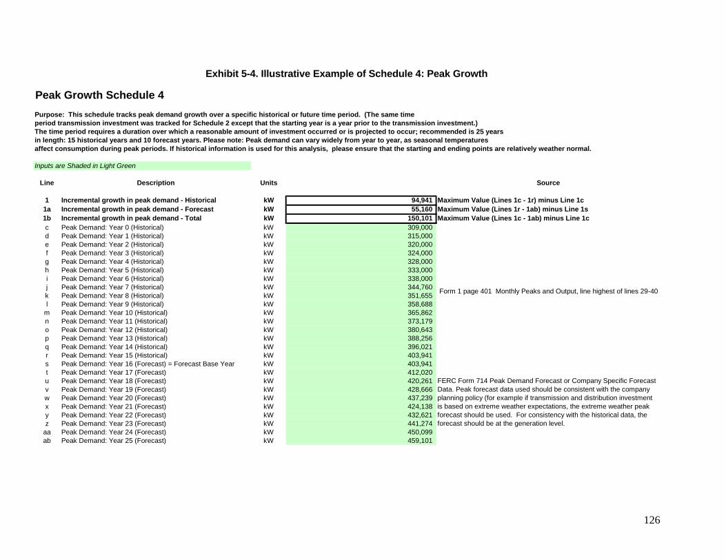
126
Exhibit 5-4. Illustrative Example of Schedule 4: Peak Growth
Peak Growth Schedule 4Purpose: This schedule tracks peak demand growth over a specific historical or future time period. (The same time period transmission investment was tracked for Schedule 2 except that the starting year is a year prior to the transmission investment.) The time period requires a duration over which a reasonable amount of investment occurred or is projected to occur; recommended is 25 years in length: 15 historical years and 10 forecast years. Please note: Peak demand can vary widely from year to year, as seasonal temperatures affect consumption during peak periods. If historical information is used for this analysis, please ensure that the starting and ending points are relatively weather normal.
Inputs are Shaded in Light Green
Line Description Units Source
1 Incremental growth in peak demand - Historical kW 94,941 Maximum Value (Lines 1c - 1r) minus Line 1c1a Incremental growth in peak demand - Forecast kW 55,160 Maximum Value (Lines 1r - 1ab) minus Line 1s1b Incremental growth in peak demand - Total kW 150,101 Maximum Value (Lines 1c - 1ab) minus Line 1cc Peak Demand: Year 0 (Historical) kW 309,000 d Peak Demand: Year 1 (Historical) kW 315,000 e Peak Demand: Year 2 (Historical) kW 320,000 f Peak Demand: Year 3 (Historical) kW 324,000 g Peak Demand: Year 4 (Historical) kW 328,000 h Peak Demand: Year 5 (Historical) kW 333,000 i Peak Demand: Year 6 (Historical) kW 338,000 j Peak Demand: Year 7 (Historical) kW 344,760 k Peak Demand: Year 8 (Historical) kW 351,655 l Peak Demand: Year 9 (Historical) kW 358,688
m Peak Demand: Year 10 (Historical) kW 365,862 n Peak Demand: Year 11 (Historical) kW 373,179 o Peak Demand: Year 12 (Historical) kW 380,643 p Peak Demand: Year 13 (Historical) kW 388,256 q Peak Demand: Year 14 (Historical) kW 396,021 r Peak Demand: Year 15 (Historical) kW 403,941 s Peak Demand: Year 16 (Forecast) = Forecast Base Year kW 403,941 t Peak Demand: Year 17 (Forecast) kW 412,020 u Peak Demand: Year 18 (Forecast) kW 420,261 v Peak Demand: Year 19 (Forecast) kW 428,666 w Peak Demand: Year 20 (Forecast) kW 437,239 x Peak Demand: Year 21 (Forecast) kW 424,138 y Peak Demand: Year 22 (Forecast) kW 432,621 z Peak Demand: Year 23 (Forecast) kW 441,274
aa Peak Demand: Year 24 (Forecast) kW 450,099 ab Peak Demand: Year 25 (Forecast) kW 459,101
FERC Form 714 Peak Demand Forecast or Company Specific Forecast Data. Peak forecast data used should be consistent with the company planning policy (for example if transmission and distribution investment is based on extreme weather expectations, the extreme weather peak forecast should be used. For consistency with the historical data, the forecast should be at the generation level.
Form 1 page 401 Monthly Peaks and Output, line highest of lines 29-40
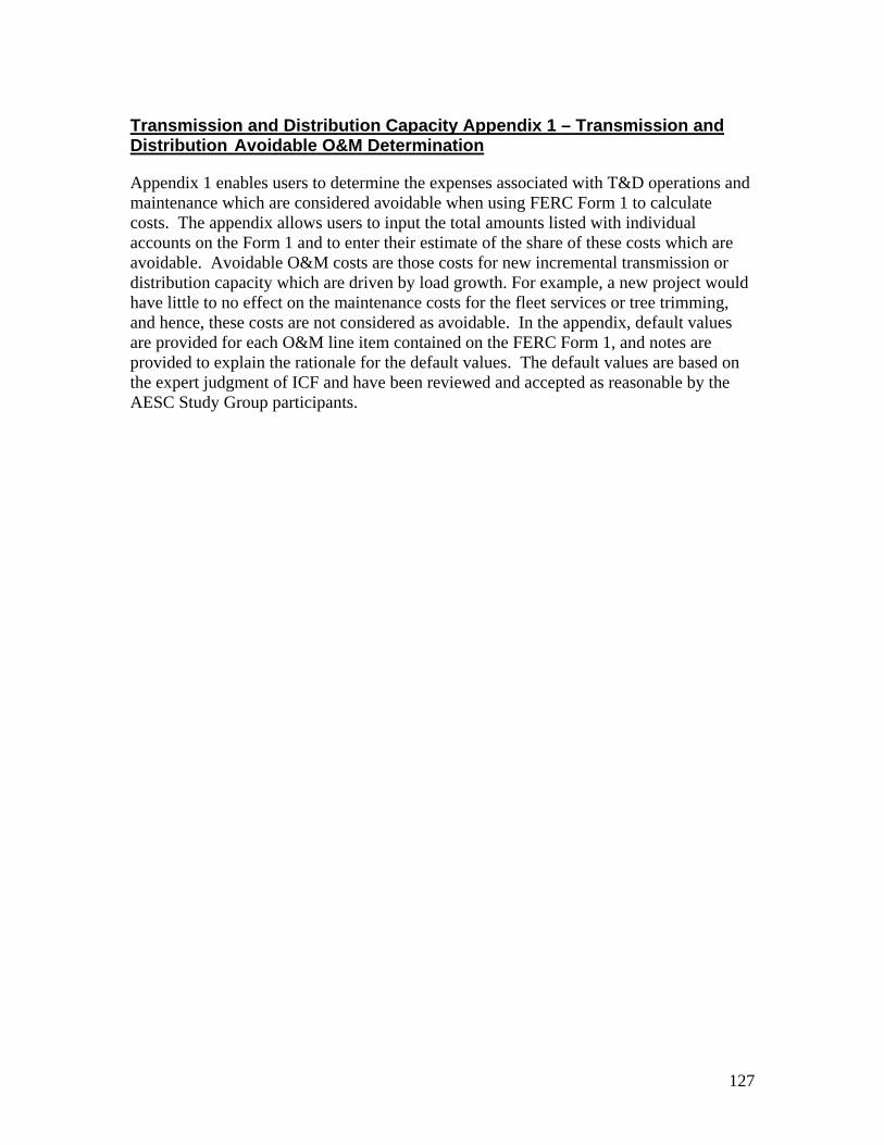
Transmission and Distribution Capacity Appendix 1 – Transmission and Distribution Avoidable O&M Determination
Appendix 1 enables users to determine the expenses associated with T&D operations and maintenance which are considered avoidable when using FERC Form 1 to calculate costs. The appendix allows users to input the total amounts listed with individual accounts on the Form 1 and to enter their estimate of the share of these costs which are avoidable. Avoidable O&M costs are those costs for new incremental transmission or distribution capacity which are driven by load growth. For example, a new project would have little to no effect on the maintenance costs for the fleet services or tree trimming, and hence, these costs are not considered as avoidable. In the appendix, default values are provided for each O&M line item contained on the FERC Form 1, and notes are provided to explain the rationale for the default values. The default values are based on the expert judgment of ICF and have been reviewed and accepted as reasonable by the AESC Study Group participants.
127
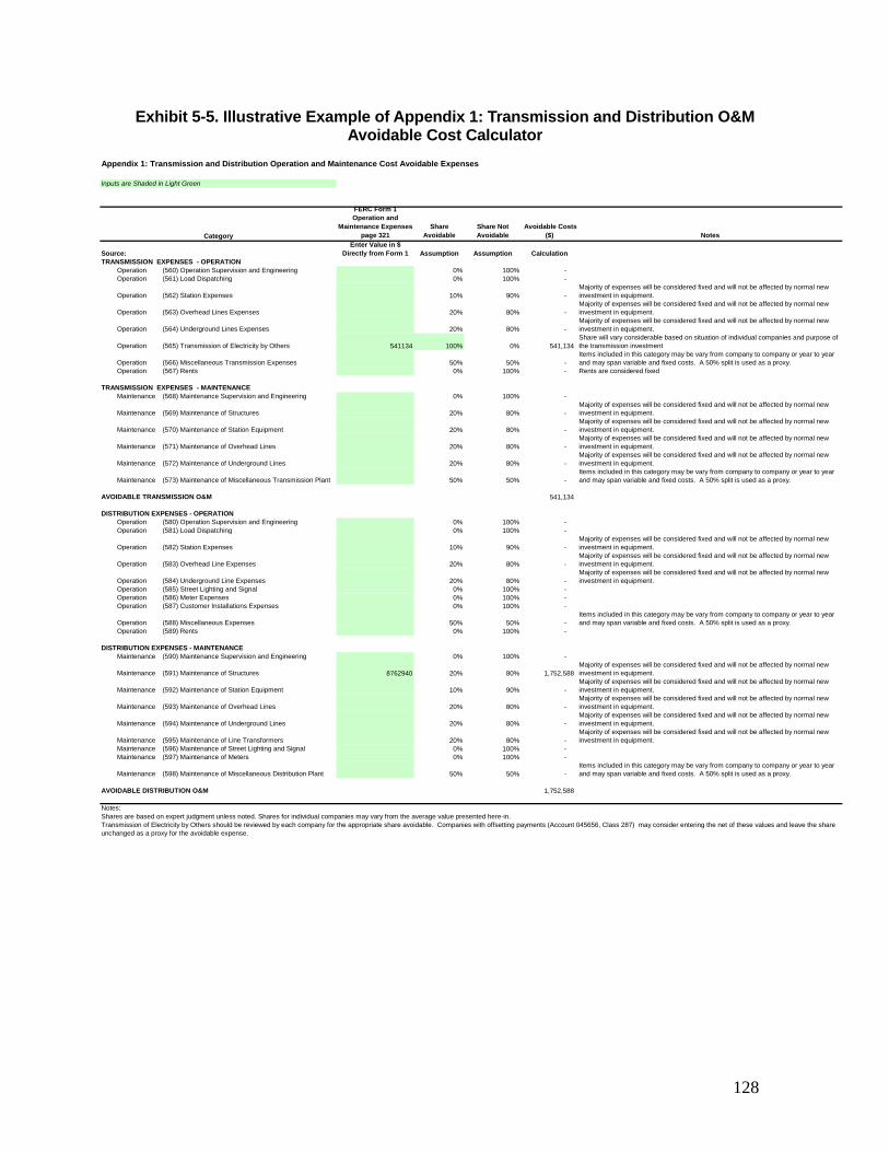
128
Exhibit 5-5. Illustrative Example of Appendix 1: Transmission and Distribution O&M Avoidable Cost Calculator
Appendix 1: Transmission and Distribution Operation and Maintenance Cost Avoidable Expenses
Inputs are Shaded in Light Green
Category
FERC Form 1 Operation and
Maintenance Expenses page 321
Share Avoidable
Share Not Avoidable
Avoidable Costs ($) Notes
Source:Enter Value in $
Directly from Form 1 Assumption Assumption CalculationTRANSMISSION EXPENSES - OPERATION
Operation (560) Operation Supervision and Engineering 0% 100% - Operation (561) Load Dispatching 0% 100% -
Operation (562) Station Expenses 10% 90% - Majority of expenses will be considered fixed and will not be affected by normal new investment in equipment.
Operation (563) Overhead Lines Expenses 20% 80% - Majority of expenses will be considered fixed and will not be affected by normal new investment in equipment.
Operation (564) Underground Lines Expenses 20% 80% - Majority of expenses will be considered fixed and will not be affected by normal new investment in equipment.
Operation (565) Transmission of Electricity by Others 541134 100% 0% 541,134 Share will vary considerable based on situation of individual companies and purpose of the transmission investment
Operation (566) Miscellaneous Transmission Expenses 50% 50% - Items included in this category may be vary from company to company or year to year and may span variable and fixed costs. A 50% split is used as a proxy.
Operation (567) Rents 0% 100% - Rents are considered fixed
TRANSMISSION EXPENSES - MAINTENANCE Maintenance (568) Maintenance Supervision and Engineering 0% 100% -
Maintenance (569) Maintenance of Structures 20% 80% - Majority of expenses will be considered fixed and will not be affected by normal new investment in equipment.
Maintenance (570) Maintenance of Station Equipment 20% 80% - Majority of expenses will be considered fixed and will not be affected by normal new investment in equipment.
Maintenance (571) Maintenance of Overhead Lines 20% 80% - Majority of expenses will be considered fixed and will not be affected by normal new investment in equipment.
Maintenance (572) Maintenance of Underground Lines 20% 80% - Majority of expenses will be considered fixed and will not be affected by normal new investment in equipment.
Maintenance (573) Maintenance of Miscellaneous Transmission Plant 50% 50% - Items included in this category may be vary from company to company or year to year and may span variable and fixed costs. A 50% split is used as a proxy.
AVOIDABLE TRANSMISSION O&M 541,134
DISTRIBUTION EXPENSES - OPERATION Operation (580) Operation Supervision and Engineering 0% 100% - Operation (581) Load Dispatching 0% 100% -
Operation (582) Station Expenses 10% 90% - Majority of expenses will be considered fixed and will not be affected by normal new investment in equipment.
Operation (583) Overhead Line Expenses 20% 80% - Majority of expenses will be considered fixed and will not be affected by normal new investment in equipment.
Operation (584) Underground Line Expenses 20% 80% - Majority of expenses will be considered fixed and will not be affected by normal new investment in equipment.
Operation (585) Street Lighting and Signal 0% 100% - Operation (586) Meter Expenses 0% 100% - Operation (587) Customer Installations Expenses 0% 100% -
Operation (588) Miscellaneous Expenses 50% 50% - Items included in this category may be vary from company to company or year to year and may span variable and fixed costs. A 50% split is used as a proxy.
Operation (589) Rents 0% 100% -
DISTRIBUTION EXPENSES - MAINTENANCE Maintenance (590) Maintenance Supervision and Engineering 0% 100% -
Maintenance (591) Maintenance of Structures 8762940 20% 80% 1,752,588 Majority of expenses will be considered fixed and will not be affected by normal new investment in equipment.
Maintenance (592) Maintenance of Station Equipment 10% 90% - Majority of expenses will be considered fixed and will not be affected by normal new investment in equipment.
Maintenance (593) Maintenance of Overhead Lines 20% 80% - Majority of expenses will be considered fixed and will not be affected by normal new investment in equipment.
Maintenance (594) Maintenance of Underground Lines 20% 80% - Majority of expenses will be considered fixed and will not be affected by normal new investment in equipment.
Maintenance (595) Maintenance of Line Transformers 20% 80% - Majority of expenses will be considered fixed and will not be affected by normal new investment in equipment.
Maintenance (596) Maintenance of Street Lighting and Signal 0% 100% - Maintenance (597) Maintenance of Meters 0% 100% -
Maintenance (598) Maintenance of Miscellaneous Distribution Plant 50% 50% - Items included in this category may be vary from company to company or year to year and may span variable and fixed costs. A 50% split is used as a proxy.
AVOIDABLE DISTRIBUTION O&M 1,752,588
Notes: Shares are based on expert judgment unless noted. Shares for individual companies may vary from the average value presented here-in.Transmission of Electricity by Others should be reviewed by each company for the appropriate share avoidable. Companies with offsetting payments (Account 045656, Class 287) may consider entering the net of these values and leave the share unchanged as a proxy for the avoidable expense.
Chapter Six: Demand Reduction Induced Price Effects In this chapter, we describe our approach to estimating potential benefits related to demand reduction induced price effects (DRIPE). The results of this analysis are presented as well. All results are presented in 2005$ unless otherwise noted.
DRIPE Benefits
Avoided costs for firm power as described in Chapter 3 represent the savings associated with reductions in demand based on the price that power (or electrical energy) would have cost absent the demand reduction.
For example, in a market where the total peak hour load is 100 kW and the marginal cost of power purchases are $30/kWyr, if a savings of 10kW is realized in that peak hour through C&LM programs, and if the supply resources are also reduced by the same 10 kW, the benefit associated with those programs is $300/yr ($30/kWyr * 10kW demand reduction). This is the equivalent of the total expenses before the demand reduction minus the expenses after the demand reduction ((100kW * $30/kWyr) – (90kW * $30/kWyr ) = $3000/yr - $2700/kWyr = $300/kWyr). This approach to determining avoided costs based on the marginal cost applies to energy as well as to capacity supply costs.
Demand reduction induced price effects (DRIPE) reflect any additional change in costs that occur due to a price response that results from the demand reduction. In the above example, if the marginal capacity price is reduced from $30/kWyr to $29/kWyr through the consumption of fewer resources, the total benefit which above was $300/yr becomes $390/yr. As above, this total benefit is calculated as the total expenses before the demand reduction minus the expenses after the demand reduction ((100kW * $30/kWyr) – (90kW * $29/kWyr ) = $3000/yr - $2610/yr = $390/yr). The direct price effect of the kW savings can be determined through isolating the savings directly attributable to the change in price which in this example is $90/yr ($390/yr - $300/yr). The $90/yr reflects the incremental benefit associated with the demand reduction attributable to the price response. This is illustrated in Exhibit 6-1 below.
129
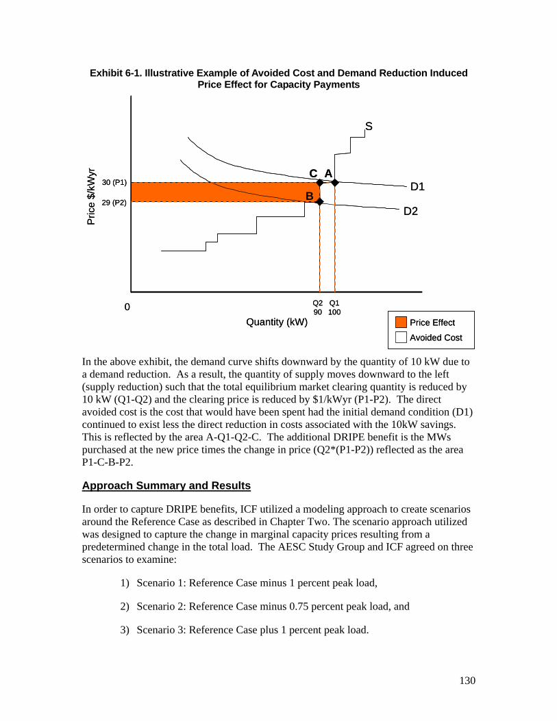
130
Exhibit 6-1. Illustrative Example of Avoided Cost and Demand Reduction Induced Price Effect for Capacity Payments
In the above exhibit, the demand curve shifts downward by the quantity of 10 kW due to a demand reduction. As a result, the quantity of supply moves downward to the left (supply reduction) such that the total equilibrium market clearing quantity is reduced by 10 kW (Q1-Q2) and the clearing price is reduced by $1/kWyr (P1-P2). The direct avoided cost is the cost that would have been spent had the initial demand condition (D1) continued to exist less the direct reduction in costs associated with the 10kW savings. This is reflected by the area A-Q1-Q2-C. The additional DRIPE benefit is the MWs purchased at the new price times the change in price (Q2*(P1-P2)) reflected as the area P1-C-B-P2.
Approach Summary and Results
In order to capture DRIPE benefits, ICF utilized a modeling approach to create scenarios around the Reference Case as described in Chapter Two. The scenario approach utilized was designed to capture the change in marginal capacity prices resulting from a predetermined change in the total load. The AESC Study Group and ICF agreed on three scenarios to examine:
1) Scenario 1: Reference Case minus 1 percent peak load,
2) Scenario 2: Reference Case minus 0.75 percent peak load, and
3) Scenario 3: Reference Case plus 1 percent peak load.
Pric
e $/
kWyr
Quantity (kW)
Q290
Q1100
30 (P1)
29 (P2)
0
S
D1
D2B
A
Price Effect
Avoided Cost
C
Pric
e $/
kWyr
Quantity (kW)
Q290
Q1100
30 (P1)
29 (P2)
0
S
D1
D2B
A
Price Effect
Avoided Cost
C

Scenarios 1 and 2 (minus 1 and 0.75 percent) were considered by the AESC Study Group as highly probable levels of peak demand reduction. Scenario 3 (plus 1 percent) was performed to demonstrate the sensitivity of the model. The percent change of peak load was meant to approximate the aggregated demand savings of the sponsors’ energy efficiency programs.
These scenarios, through their design to reduce peak load only, focus on the change in capacity price and out-of-market costs. ICF conducted an additional scenario analysis that included a 1 percent reduction for all hours (8760 hours) of the year to reflect the potential change in energy as well. Since this analysis did not reflect significant changes in the marginal energy values, it was not utilized for the calculation of DRIPE.
In all the scenario analyses, all zones were considered to have simultaneous load reductions of the same percentage. The scenarios utilized the same modeling construct as the Reference Case and as such reflect zonal price results directly comparable to that of the Reference Case.
The AESC Study Group reviewed the energy and capacity price results of the sensitivities and decided that the preferred scenario to estimate the benefits due to DRIPE to be Scenario 2 (0.75 percent reduction). Based on the design of the scenarios, the DRIPE measures only the effect of permanent demand reductions. The scenarios reflect a shift in the LICAP demand curve that results from measurable energy efficiency programs affecting peak demand. As such, the DRIPE effect does not consider short-term demand responsiveness either directly in the energy markets or related to temporary load response (such as OP4 events) or other demand response programs. DRIPE values should only be applied to demand savings from energy efficiency programs and not demand response or distributed generation.
The DRIPE benefits for all of New England are shown in Exhibit 6-2 below. These benefits are incremental and therefore additive to the avoided capacity values presented in Chapter 3. The New England DRIPE benefits represent the sum of the zonal benefits. These values are presented for reference purposes only and not for use in the screening tools. Zonal DRIPE benefits, for use in the screening tools, are presented in Appendix 2.
131
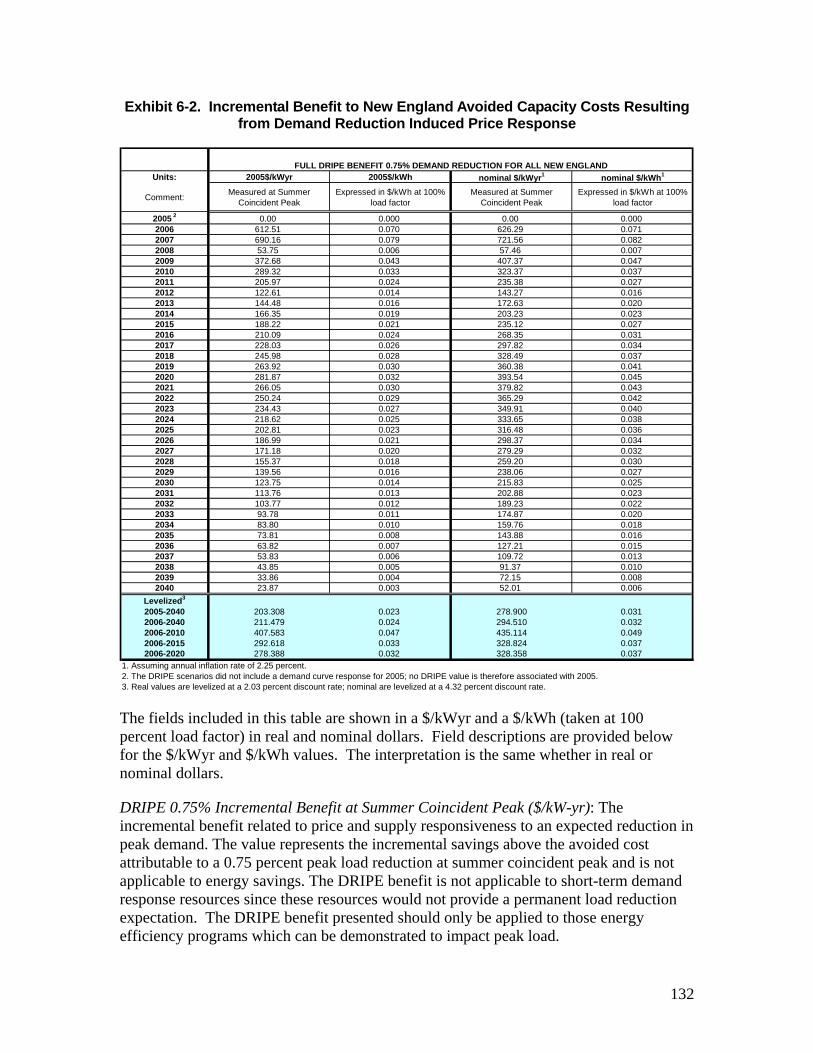
Exhibit 6-2. Incremental Benefit to New England Avoided Capacity Costs Resulting from Demand Reduction Induced Price Response
Units: 2005$/kWyr 2005$/kWh nominal $/kWyr1 nominal $/kWh1
Comment: Measured at Summer Coincident Peak
Expressed in $/kWh at 100% load factor
Measured at Summer Coincident Peak
Expressed in $/kWh at 100% load factor
2005 2 0.00 0.000 0.00 0.0002006 612.51 0.070 626.29 0.0712007 690.16 0.079 721.56 0.0822008 53.75 0.006 57.46 0.0072009 372.68 0.043 407.37 0.0472010 289.32 0.033 323.37 0.0372011 205.97 0.024 235.38 0.0272012 122.61 0.014 143.27 0.0162013 144.48 0.016 172.63 0.0202014 166.35 0.019 203.23 0.0232015 188.22 0.021 235.12 0.0272016 210.09 0.024 268.35 0.0312017 228.03 0.026 297.82 0.0342018 245.98 0.028 328.49 0.0372019 263.92 0.030 360.38 0.0412020 281.87 0.032 393.54 0.0452021 266.05 0.030 379.82 0.0432022 250.24 0.029 365.29 0.0422023 234.43 0.027 349.91 0.0402024 218.62 0.025 333.65 0.0382025 202.81 0.023 316.48 0.0362026 186.99 0.021 298.37 0.0342027 171.18 0.020 279.29 0.0322028 155.37 0.018 259.20 0.0302029 139.56 0.016 238.06 0.0272030 123.75 0.014 215.83 0.0252031 113.76 0.013 202.88 0.0232032 103.77 0.012 189.23 0.0222033 93.78 0.011 174.87 0.0202034 83.80 0.010 159.76 0.0182035 73.81 0.008 143.88 0.0162036 63.82 0.007 127.21 0.0152037 53.83 0.006 109.72 0.0132038 43.85 0.005 91.37 0.0102039 33.86 0.004 72.15 0.0082040 23.87 0.003 52.01 0.006
Levelized3
2005-2040 203.308 0.023 278.900 0.0312006-2040 211.479 0.024 294.510 0.0322006-2010 407.583 0.047 435.114 0.0492006-2015 292.618 0.033 328.824 0.0372006-2020 278.388 0.032 328.358 0.037
1. Assuming annual inflation rate of 2.25 percent.2. The DRIPE scenarios did not include a demand curve response for 2005; no DRIPE value is therefore associated with 2005.3. Real values are levelized at a 2.03 percent discount rate; nominal are levelized at a 4.32 percent discount rate.
FULL DRIPE BENEFIT 0.75% DEMAND REDUCTION FOR ALL NEW ENGLAND
The fields included in this table are shown in a $/kWyr and a $/kWh (taken at 100 percent load factor) in real and nominal dollars. Field descriptions are provided below for the $/kWyr and $/kWh values. The interpretation is the same whether in real or nominal dollars.
DRIPE 0.75% Incremental Benefit at Summer Coincident Peak ($/kW-yr): The incremental benefit related to price and supply responsiveness to an expected reduction in peak demand. The value represents the incremental savings above the avoided cost attributable to a 0.75 percent peak load reduction at summer coincident peak and is not applicable to energy savings. The DRIPE benefit is not applicable to short-term demand response resources since these resources would not provide a permanent load reduction expectation. The DRIPE benefit presented should only be applied to those energy efficiency programs which can be demonstrated to impact peak load.
132
DRIPE 0.75% Capacity Price ($/kWh): The annual avoided costs for DRIPE are converted to $/kWh at 100 percent load factor. This field represents the average savings for every hour (8760 hours). This value reflects only capacity savings and should not be applied to potential energy savings. This value is presented for informational purposes only at the request of the Study Group.
Scope of the Analysis
In general, the DRIPE equilibrium capacity benefit analysis presented herein is not conservative in nature because of the assumptions driving the results. The analysis assumes that the DRIPE benefit based on the savings in total expenditures for capacity is realized immediately once the demand savings are realized. However, two contributing factors may delay the responsiveness. First, since the energy efficiency benefits must be demonstrated before they are recognized as a coincident peak reduction, the benefit would be delayed up to one year if the LICAP peak demand curve is set annually. That is, the peak reduction and associated shift in the demand curve would be recognized only after the fact, delaying the price responsiveness until the point at which a new demand curve is established. Second, since approximately 90 percent of the current demand for capacity is satisfied through bilateral contracts, one would expect that some lagged effect would be in place to the extent that those contracts are not indexed to the market. As the LICAP market matures and existing contracts expire and are replaced by new agreements, the lag would become more and more abbreviated.
In addition, the DRIPE benefit captures both the direct price effect (illustrated in Exhibit 6-1) and the potential effect associated with reducing the requirement for reliability must run (RMR) units. Since RMR units are considered as required units to maintain system stability in peak conditions, a measurable reduction in peak demand will affect the need for these units. Hence the costs of maintaining these units to load serving entities has the potential to be reduced through demand savings and is included in the DRIPE values presented for coincident peak savings.
To some extent, this lack of conservatism is countered by the narrow scope considered for DRIPE. As discussed earlier, the DRIPE analysis does not consider the potential for price responsiveness in the energy markets and as such may understate the total benefit. Also, the choice of use of the demand reduction of 0.75%, as opposed to 1.0%, was a conservative assumption. However, the assumptions reflecting the immediate realization of the DRIPE benefit are by far the dominant assumption.
Since this analysis did not measure the potential lag effects on the DRIPE benefit, an alternate benefit calculation, which the Study Group termed “DRIPE Light”, was calculated and is presented in the following section. This is followed by a discussion of the methodology used to calculate the Incremental DRIPE effect.
133
DRIPE Light Benefits
The DRIPE benefits presented in Exhibit 6-2 represent the capacity payments that would be saved if all load cleared in the spot market. Since many load serving entities currently have bilateral contracts in place and are expected to cover positions at least to some extent going forward, it is possible that Load Serving Entities (LSE) may not be able to realize the full price response associated with demand reduction. DRIPE Light assumes that only those capacity transactions which occur on the spot market are able to realize the savings associated with price response. To estimate the share of capacity cleared in the spot market, ICF relied on the ISO New England’s 2004 Annual Markets Report and the ISO New York annual market reports, which indicated that roughly 10 percent of the market transacted in the spot market. Based on this information, the DRIPE savings were calculated for only 10 percent of the total MW.
Savings under DRIPE Light may also affect out-of-market costs. Unlike capacity prices, the out-of-market savings associated with the peak demand reductions in the DRIPE Light scenario are equivalent to those in the full DRIPE scenario.
DRIPE Light is a much more conservative approximation of DRIPE than is the “Full DRIPE” scenario. Although it is likely that bilateral transactions will continue to occur for capacity transactions, it is also likely that these contracts will be indexed to the market in some form or will be shorter-term transactions. As such, it is unlikely that all capacity currently contracted bilaterally will be unaffected should spot market capacity clearing prices fall due to demand reductions over the long-term horizon of this study. It is more likely that all capacity will be affected to some extent, but even the capacity which is contracted bilaterally will experience some lagging effect following the spot market changes. Given the confidential nature of bilateral contracts, it is not possible to estimate without significant research or broad based assumptions, the quantity of capacity with long-term contracts that are currently indexed to market. Nor is it possible to estimate the term periods associated with current contracts.
DRIPE Light savings are presented in Exhibit 6-3 for all of New England for reference purposes. Zonal savings to be used in the screening models are presented in Appendix 2.
134
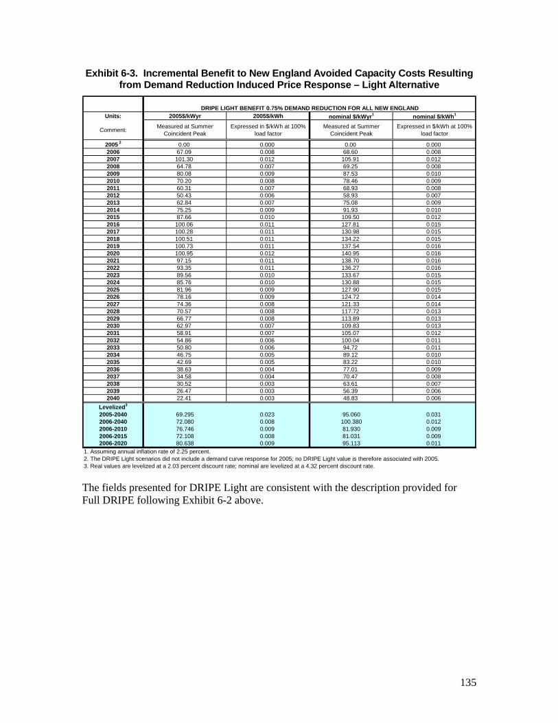
Exhibit 6-3. Incremental Benefit to New England Avoided Capacity Costs Resulting from Demand Reduction Induced Price Response – Light Alternative
Units: 2005$/kWyr 2005$/kWh nominal $/kWyr1 nominal $/kWh1
Comment: Measured at Summer Coincident Peak
Expressed in $/kWh at 100% load factor
Measured at Summer Coincident Peak
Expressed in $/kWh at 100% load factor
2005 2 0.00 0.000 0.00 0.0002006 67.09 0.008 68.60 0.0082007 101.30 0.012 105.91 0.0122008 64.78 0.007 69.25 0.0082009 80.08 0.009 87.53 0.0102010 70.20 0.008 78.46 0.0092011 60.31 0.007 68.93 0.0082012 50.43 0.006 58.93 0.0072013 62.84 0.007 75.08 0.0092014 75.25 0.009 91.93 0.0102015 87.66 0.010 109.50 0.0122016 100.06 0.011 127.81 0.0152017 100.28 0.011 130.98 0.0152018 100.51 0.011 134.22 0.0152019 100.73 0.011 137.54 0.0162020 100.95 0.012 140.95 0.0162021 97.15 0.011 138.70 0.0162022 93.35 0.011 136.27 0.0162023 89.56 0.010 133.67 0.0152024 85.76 0.010 130.88 0.0152025 81.96 0.009 127.90 0.0152026 78.16 0.009 124.72 0.0142027 74.36 0.008 121.33 0.0142028 70.57 0.008 117.72 0.0132029 66.77 0.008 113.89 0.0132030 62.97 0.007 109.83 0.0132031 58.91 0.007 105.07 0.0122032 54.86 0.006 100.04 0.0112033 50.80 0.006 94.72 0.0112034 46.75 0.005 89.12 0.0102035 42.69 0.005 83.22 0.0102036 38.63 0.004 77.01 0.0092037 34.58 0.004 70.47 0.0082038 30.52 0.003 63.61 0.0072039 26.47 0.003 56.39 0.0062040 22.41 0.003 48.83 0.006
Levelized3
2005-2040 69.295 0.023 95.060 0.0312006-2040 72.080 0.008 100.380 0.0122006-2010 76.746 0.009 81.930 0.0092006-2015 72.108 0.008 81.031 0.0092006-2020 80.638 0.009 95.113 0.011
1. Assuming annual inflation rate of 2.25 percent.2. The DRIPE Light scenarios did not include a demand curve response for 2005; no DRIPE Light value is therefore associated with 2005.3. Real values are levelized at a 2.03 percent discount rate; nominal are levelized at a 4.32 percent discount rate.
DRIPE LIGHT BENEFIT 0.75% DEMAND REDUCTION FOR ALL NEW ENGLAND
The fields presented for DRIPE Light are consistent with the description provided for Full DRIPE following Exhibit 6-2 above.
135
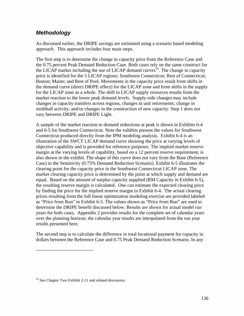
Methodology
As discussed earlier, the DRIPE savings are estimated using a scenario based modeling approach. This approach includes four main steps.
The first step is to determine the change in capacity price from the Reference Case and the 0.75 percent Peak Demand Reduction Case. Both cases rely on the same construct for the LICAP market including the use of LICAP demand curves16. The change in capacity price is identified for the 5 LICAP regions: Southwest Connecticut; Rest of Connecticut; Boston; Maine; and Rest of Pool. Movements in the capacity price result from shifts in the demand curve (direct DRIPE effect) for the LICAP zone and from shifts in the supply for the LICAP zone as a whole. The shift in LICAP supply resources results from the market reaction to the lower peak demand levels. Supply-side changes may include changes in capacity transfers across regions, changes in unit retirements; change in mothball activity; and/or changes in the construction of new capacity. Step 1 does not vary between DRIPE and DRIPE Light.
A sample of the market reaction to demand reductions at peak is shown in Exhibits 6-4 and 6-5 for Southwest Connecticut. Note the exhibits present the values for Southwest Connecticut produced directly from the IPM modeling analysis. Exhibit 6-4 is an illustration of the SWCT LICAP demand curve showing the price at varying levels of objective capability and is provided for reference purposes. The implied market reserve margin at the varying levels of capability, based on a 12 percent reserve requirement, is also shown in the exhibit. The shape of this curve does not vary from the Base (Reference Case) to the Sensitivity (0.75% Demand Reduction Scenario). Exhibit 6-5 illustrates the clearing point for the capacity price in the Southwest Connecticut LICAP zone. The market clearing capacity price is determined by the point at which supply and demand are equal. Based on the amount of surplus capacity supplied (RM Capacity in Exhibit 6-5), the resulting reserve margin is calculated. One can estimate the expected clearing price by finding the price for the implied reserve margin in Exhibit 6-4. The actual clearing prices resulting form the full linear optimization modeling exercise are provided labeled as “Price from Run” in Exhibit 6-5. The values shown as “Price from Run” are used to determine the DRIPE benefit discussed below. Results are shown for actual model run years for both cases. Appendix 2 provides results for the complete set of calendar years over the planning horizon; the calendar year results are interpolated from the run year results presented here.
The second step is to calculate the difference in total locational payment for capacity in dollars between the Reference Case and 0.75 Peak Demand Reduction Scenario. In any
16 See Chapter Two Exhibit 2-11 and related discussion.
136
given scenario, this total payment is calculated as the megawatts of supply side resources multiplied by the capacity price (“Price from Run” in Exhibit 6-5). The difference between the total capacity payment in each scenario is then calculated (shown as column h in Exhibit 6-6). This total benefit is comprised of two key components: 1) the avoided cost associated with the demand reduction (area A-Q1-Q2-C in Exhibit 6-1); and 2) the price response effect. The avoided cost is calculated as the total load reduction times the initial Reference Case price (column (i) in Exhibit 6-6). To determine the price response effect, the avoided cost is subtracted from the total benefit identified earlier (column (h) – column (i) in Exhibit 6-6). Alternately, one can isolate the price effect as the new supply quantity times the change in price. However, since the avoided costs are measured using the change in demand rather than the change in the market clearing quantity of capacity17, one must also determine if any indirect effects are present that contribute to DRIPE related to changes in the supply. These calculations are illustrated in Exhibit 6-6 for the full DRIPE scenario for Southwest Connecticut.
17 Under the LICAP design a change in the peak demand for capacity will not necessarily result in the same change in the quantity of capacity cleared in the marketplace. That is, since the reserve margin is not required to be constant, the change in the quantity of capacity supplied at the equilibrium price may vary from the change in demand.
137
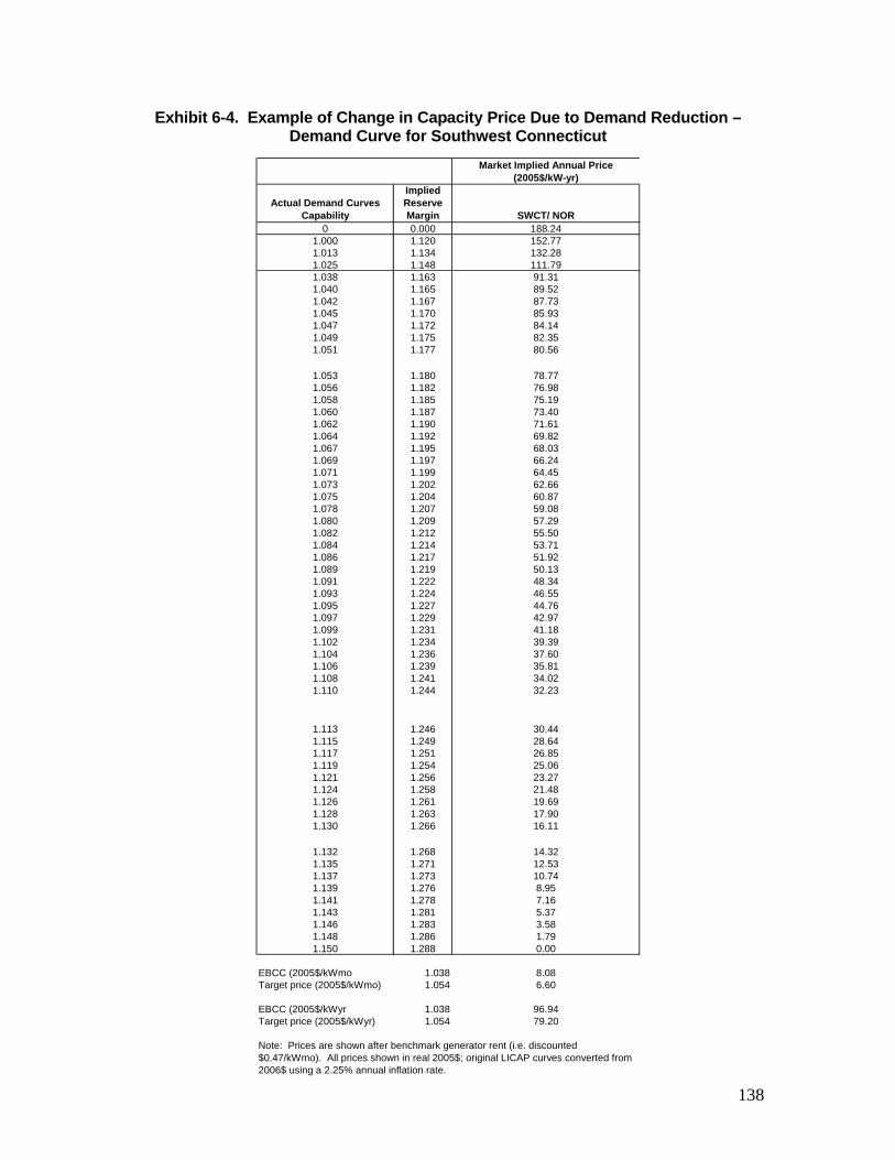
138
Exhibit 6-4. Example of Change in Capacity Price Due to Demand Reduction – Demand Curve for Southwest Connecticut
Actual Demand Curves Capability
Implied Reserve Margin SWCT/ NOR
0 0.000 188.241.000 1.120 152.771.013 1.134 132.281.025 1.148 111.791.038 1.163 91.311.040 1.165 89.521.042 1.167 87.731.045 1.170 85.931.047 1.172 84.141.049 1.175 82.351.051 1.177 80.56
1.053 1.180 78.771.056 1.182 76.981.058 1.185 75.191.060 1.187 73.401.062 1.190 71.611.064 1.192 69.821.067 1.195 68.031.069 1.197 66.241.071 1.199 64.451.073 1.202 62.661.075 1.204 60.871.078 1.207 59.081.080 1.209 57.291.082 1.212 55.501.084 1.214 53.711.086 1.217 51.921.089 1.219 50.131.091 1.222 48.341.093 1.224 46.551.095 1.227 44.761.097 1.229 42.971.099 1.231 41.181.102 1.234 39.391.104 1.236 37.601.106 1.239 35.811.108 1.241 34.021.110 1.244 32.23
1.113 1.246 30.441.115 1.249 28.641.117 1.251 26.851.119 1.254 25.061.121 1.256 23.271.124 1.258 21.481.126 1.261 19.691.128 1.263 17.901.130 1.266 16.11
1.132 1.268 14.321.135 1.271 12.531.137 1.273 10.741.139 1.276 8.951.141 1.278 7.161.143 1.281 5.371.146 1.283 3.581.148 1.286 1.791.150 1.288 0.00
EBCC (2005$/kWmo 1.038 8.08Target price (2005$/kWmo) 1.054 6.60
EBCC (2005$/kWyr 1.038 96.94Target price (2005$/kWyr) 1.054 79.20
Market Implied Annual Price (2005$/kW-yr)
Note: Prices are shown after benchmark generator rent (i.e. discounted $0.47/kWmo). All prices shown in real 2005$; original LICAP curves converted from 2006$ using a 2.25% annual inflation rate.
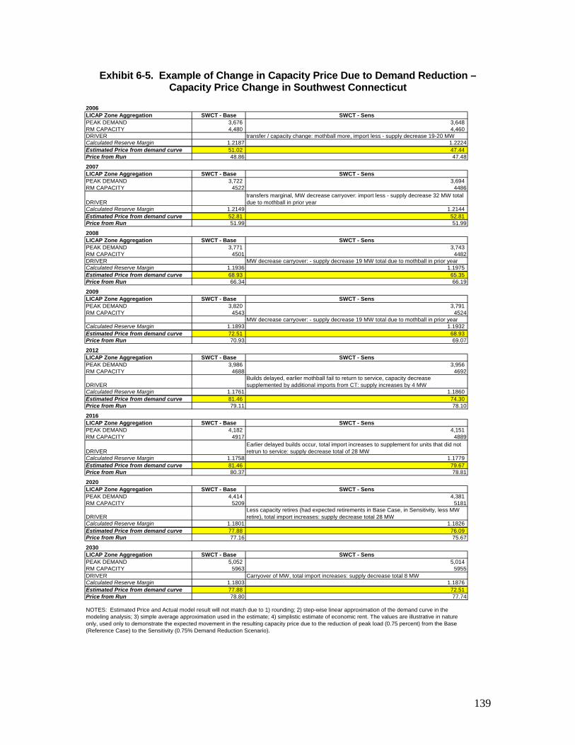
Exhibit 6-5. Example of Change in Capacity Price Due to Demand Reduction – Capacity Price Change in Southwest Connecticut
2006LICAP Zone Aggregation SWCT - Base SWCT - SensPEAK DEMAND 3,676 3,648 RM CAPACITY 4,480 4,460 DRIVER transfer / capacity change: mothball more, import less - supply decrease 19-20 MWCalculated Reserve Margin 1.2187 1.2224Estimated Price from demand curve 51.02 47.44 Price from Run 48.86 47.48
2007LICAP Zone Aggregation SWCT - Base SWCT - SensPEAK DEMAND 3,722 3,694 RM CAPACITY 4522 4486
DRIVERtransfers marginal, MW decrease carryover: import less - supply decrease 32 MW total due to mothball in prior year
Calculated Reserve Margin 1.2149 1.2144 Estimated Price from demand curve 52.81 52.81 Price from Run 51.99 51.99
2008LICAP Zone Aggregation SWCT - Base SWCT - SensPEAK DEMAND 3,771 3,743 RM CAPACITY 4501 4482DRIVER MW decrease carryover: - supply decrease 19 MW total due to mothball in prior yearCalculated Reserve Margin 1.1936 1.1975 Estimated Price from demand curve 68.93 65.35 Price from Run 66.34 66.19
2009LICAP Zone Aggregation SWCT - Base SWCT - SensPEAK DEMAND 3,820 3,791 RM CAPACITY 4543 4524
MW decrease carryover: - supply decrease 19 MW total due to mothball in prior yearCalculated Reserve Margin 1.1893 1.1932 Estimated Price from demand curve 72.51 68.93 Price from Run 70.93 69.07
2012LICAP Zone Aggregation SWCT - Base SWCT - SensPEAK DEMAND 3,986 3,956 RM CAPACITY 4688 4692
DRIVERBuilds delayed, earlier mothball fail to return to service, capacity decrease supplemented by additional imports from CT: supply increases by 4 MW
Calculated Reserve Margin 1.1761 1.1860 Estimated Price from demand curve 81.46 74.30 Price from Run 79.11 78.10
2016LICAP Zone Aggregation SWCT - Base SWCT - SensPEAK DEMAND 4,182 4,151 RM CAPACITY 4917 4889
DRIVEREarlier delayed builds occur, total import increases to supplement for units that did not retrun to service: supply decrease total of 28 MW
Calculated Reserve Margin 1.1758 1.1779 Estimated Price from demand curve 81.46 79.67 Price from Run 80.37 78.81
2020LICAP Zone Aggregation SWCT - Base SWCT - SensPEAK DEMAND 4,414 4,381 RM CAPACITY 5209 5181
DRIVERLess capacity retires (had expected retirements in Base Case, in Sensitivity, less MW retire), total import increases: supply decrease total 28 MW
Calculated Reserve Margin 1.1801 1.1826 Estimated Price from demand curve 77.88 76.09 Price from Run 77.16 75.67
2030LICAP Zone Aggregation SWCT - Base SWCT - SensPEAK DEMAND 5,052 5,014 RM CAPACITY 5963 5955DRIVER Carryover of MW, total import increases: supply decrease total 8 MWCalculated Reserve Margin 1.1803 1.1876 Estimated Price from demand curve 77.88 72.51 Price from Run 78.80 77.74
NOTES: Estimated Price and Actual model result will not match due to 1) rounding; 2) step-wise linear approximation of the demand curve in the modeling analysis; 3) simple average approximation used in the estimate; 4) simplistic estimate of economic rent. The values are illustrative in nature only, used only to demonstrate the expected movement in the resulting capacity price due to the reduction of peak load (0.75 percent) from the Base (Reference Case) to the Sensitivity (0.75% Demand Reduction Scenario).
139
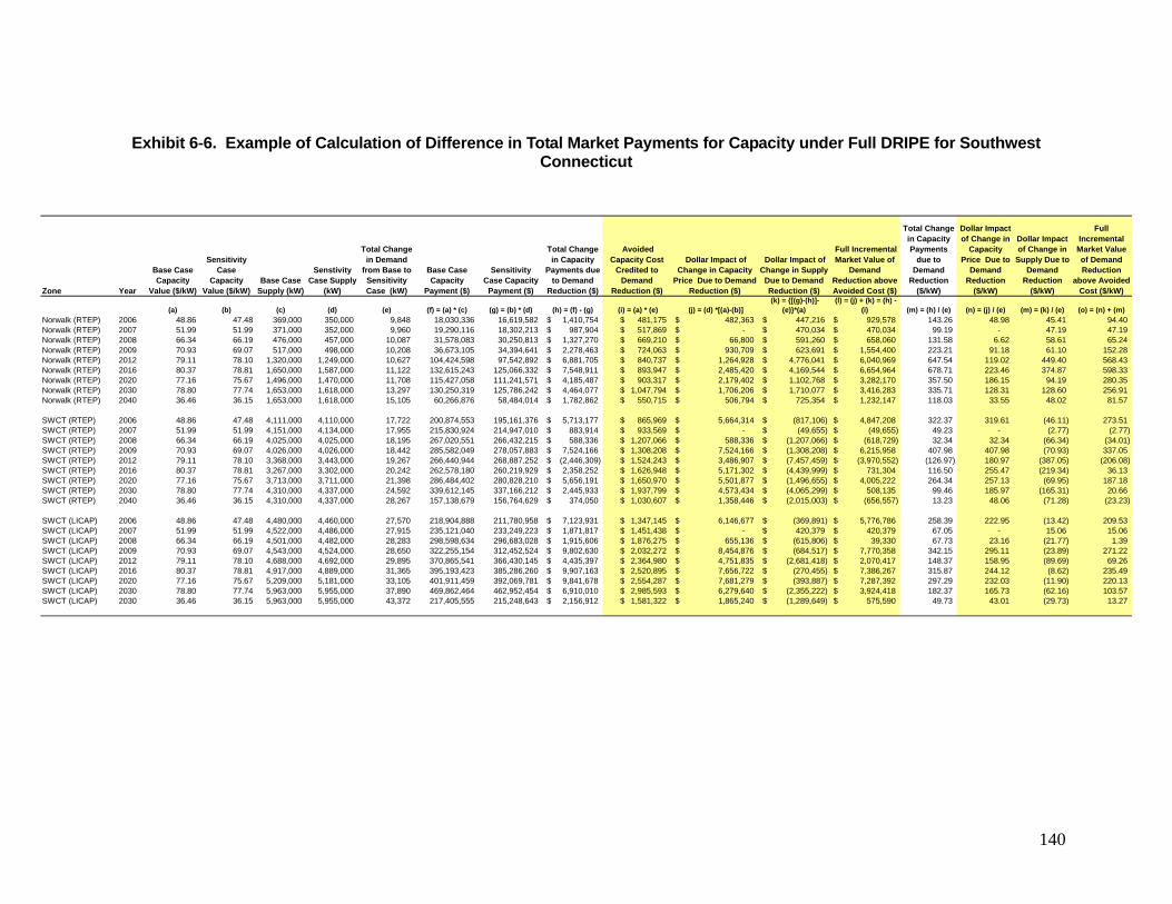
140
Exhibit 6-6. Example of Calculation of Difference in Total Market Payments for Capacity under Full DRIPE for Southwest Connecticut
Zone Year
Base Case Capacity
Value ($/kW)
Sensitivity Case
Capacity Value ($/kW)
Base Case Supply (kW)
Senstivity Case Supply
(kW)
Total Change in Demand
from Base to Sensitivity Case (kW)
Base Case Capacity
Payment ($)
Sensitivity Case Capacity
Payment ($)
Total Change in Capacity
Payments due to Demand
Reduction ($)
Avoided Capacity Cost
Credited to Demand
Reduction ($)
Dollar Impact of Change in Capacity
Price Due to Demand Reduction ($)
Dollar Impact of Change in Supply Due to Demand Reduction ($)
Full Incremental Market Value of
Demand Reduction above Avoided Cost ($)
Total Change in Capacity Payments
due to Demand
Reduction ($/kW)
Dollar Impact of Change in
Capacity Price Due to
Demand Reduction
($/kW)
Dollar Impact of Change in
Supply Due to Demand
Reduction ($/kW)
Full Incremental Market Value of Demand Reduction
above Avoided Cost ($/kW)
(a) (b) (c) (d) (e) (f) = (a) * (c) (g) = (b) * (d) (h) = (f) - (g) (i) = (a) * (e) (j) = (d) *[(a)-(b)] (k) = {[(g)-(h)]-
(e)}*(a) (l) = (j) + (k) = (h) -
(i) (m) = (h) / (e) (n) = (j) / (e) (m) = (k) / (e) (o) = (n) + (m)Norwalk (RTEP) 2006 48.86 47.48 369,000 350,000 9,848 18,030,336 16,619,582 1,410,754$ 481,175$ 482,363$ 447,216$ 929,578$ 143.26 48.98 45.41 94.40 Norwalk (RTEP) 2007 51.99 51.99 371,000 352,000 9,960 19,290,116 18,302,213 987,904$ 517,869$ -$ 470,034$ 470,034$ 99.19 - 47.19 47.19 Norwalk (RTEP) 2008 66.34 66.19 476,000 457,000 10,087 31,578,083 30,250,813 1,327,270$ 669,210$ 66,800$ 591,260$ 658,060$ 131.58 6.62 58.61 65.24 Norwalk (RTEP) 2009 70.93 69.07 517,000 498,000 10,208 36,673,105 34,394,641 2,278,463$ 724,063$ 930,709$ 623,691$ 1,554,400$ 223.21 91.18 61.10 152.28 Norwalk (RTEP) 2012 79.11 78.10 1,320,000 1,249,000 10,627 104,424,598 97,542,892 6,881,705$ 840,737$ 1,264,928$ 4,776,041$ 6,040,969$ 647.54 119.02 449.40 568.43 Norwalk (RTEP) 2016 80.37 78.81 1,650,000 1,587,000 11,122 132,615,243 125,066,332 7,548,911$ 893,947$ 2,485,420$ 4,169,544$ 6,654,964$ 678.71 223.46 374.87 598.33 Norwalk (RTEP) 2020 77.16 75.67 1,496,000 1,470,000 11,708 115,427,058 111,241,571 4,185,487$ 903,317$ 2,179,402$ 1,102,768$ 3,282,170$ 357.50 186.15 94.19 280.35 Norwalk (RTEP) 2030 78.80 77.74 1,653,000 1,618,000 13,297 130,250,319 125,786,242 4,464,077$ 1,047,794$ 1,706,206$ 1,710,077$ 3,416,283$ 335.71 128.31 128.60 256.91 Norwalk (RTEP) 2040 36.46 36.15 1,653,000 1,618,000 15,105 60,266,876 58,484,014 1,782,862$ 550,715$ 506,794$ 725,354$ 1,232,147$ 118.03 33.55 48.02 81.57
SWCT (RTEP) 2006 48.86 47.48 4,111,000 4,110,000 17,722 200,874,553 195,161,376 5,713,177$ 865,969$ 5,664,314$ (817,106)$ 4,847,208$ 322.37 319.61 (46.11) 273.51 SWCT (RTEP) 2007 51.99 51.99 4,151,000 4,134,000 17,955 215,830,924 214,947,010 883,914$ 933,569$ -$ (49,655)$ (49,655)$ 49.23 - (2.77) (2.77) SWCT (RTEP) 2008 66.34 66.19 4,025,000 4,025,000 18,195 267,020,551 266,432,215 588,336$ 1,207,066$ 588,336$ (1,207,066)$ (618,729)$ 32.34 32.34 (66.34) (34.01) SWCT (RTEP) 2009 70.93 69.07 4,026,000 4,026,000 18,442 285,582,049 278,057,883 7,524,166$ 1,308,208$ 7,524,166$ (1,308,208)$ 6,215,958$ 407.98 407.98 (70.93) 337.05 SWCT (RTEP) 2012 79.11 78.10 3,368,000 3,443,000 19,267 266,440,944 268,887,252 (2,446,309)$ 1,524,243$ 3,486,907$ (7,457,459)$ (3,970,552)$ (126.97) 180.97 (387.05) (206.08) SWCT (RTEP) 2016 80.37 78.81 3,267,000 3,302,000 20,242 262,578,180 260,219,929 2,358,252$ 1,626,948$ 5,171,302$ (4,439,999)$ 731,304$ 116.50 255.47 (219.34) 36.13 SWCT (RTEP) 2020 77.16 75.67 3,713,000 3,711,000 21,398 286,484,402 280,828,210 5,656,191$ 1,650,970$ 5,501,877$ (1,496,655)$ 4,005,222$ 264.34 257.13 (69.95) 187.18 SWCT (RTEP) 2030 78.80 77.74 4,310,000 4,337,000 24,592 339,612,145 337,166,212 2,445,933$ 1,937,799$ 4,573,434$ (4,065,299)$ 508,135$ 99.46 185.97 (165.31) 20.66 SWCT (RTEP) 2040 36.46 36.15 4,310,000 4,337,000 28,267 157,138,679 156,764,629 374,050$ 1,030,607$ 1,358,446$ (2,015,003)$ (656,557)$ 13.23 48.06 (71.28) (23.23)
SWCT (LICAP) 2006 48.86 47.48 4,480,000 4,460,000 27,570 218,904,888 211,780,958 7,123,931$ 1,347,145$ 6,146,677$ (369,891)$ 5,776,786$ 258.39 222.95 (13.42) 209.53 SWCT (LICAP) 2007 51.99 51.99 4,522,000 4,486,000 27,915 235,121,040 233,249,223 1,871,817$ 1,451,438$ -$ 420,379$ 420,379$ 67.05 - 15.06 15.06 SWCT (LICAP) 2008 66.34 66.19 4,501,000 4,482,000 28,283 298,598,634 296,683,028 1,915,606$ 1,876,275$ 655,136$ (615,806)$ 39,330$ 67.73 23.16 (21.77) 1.39 SWCT (LICAP) 2009 70.93 69.07 4,543,000 4,524,000 28,650 322,255,154 312,452,524 9,802,630$ 2,032,272$ 8,454,876$ (684,517)$ 7,770,358$ 342.15 295.11 (23.89) 271.22 SWCT (LICAP) 2012 79.11 78.10 4,688,000 4,692,000 29,895 370,865,541 366,430,145 4,435,397$ 2,364,980$ 4,751,835$ (2,681,418)$ 2,070,417$ 148.37 158.95 (89.69) 69.26 SWCT (LICAP) 2016 80.37 78.81 4,917,000 4,889,000 31,365 395,193,423 385,286,260 9,907,163$ 2,520,895$ 7,656,722$ (270,455)$ 7,386,267$ 315.87 244.12 (8.62) 235.49 SWCT (LICAP) 2020 77.16 75.67 5,209,000 5,181,000 33,105 401,911,459 392,069,781 9,841,678$ 2,554,287$ 7,681,279$ (393,887)$ 7,287,392$ 297.29 232.03 (11.90) 220.13 SWCT (LICAP) 2030 78.80 77.74 5,963,000 5,955,000 37,890 469,862,464 462,952,454 6,910,010$ 2,985,593$ 6,279,640$ (2,355,222)$ 3,924,418$ 182.37 165.73 (62.16) 103.57 SWCT (LICAP) 2030 36.46 36.15 5,963,000 5,955,000 43,372 217,405,555 215,248,643 2,156,912$ 1,581,322$ 1,865,240$ (1,289,649)$ 575,590$ 49.73 43.01 (29.73) 13.27

The third step of the DRIPE calculation is to determine if any change in out-of-market costs occurs between the two scenarios and how much of this change is considered incremental to the avoided cost. Any incremental benefit will be directly related to a cost savings in the out-of-market expenses rather than a price response in the market. The out-of-market cost determination is consistent in the Reference and the 0.75 percent Peak Demand Reduction Cases and utilizes the methodology described in Chapter 3. Since out-of-market costs are independent of the megawatts cleared in the spot and bilateral markets, these costs do not vary across the DRIPE and DRIPE Light benefit. The per kilowatt dollar value is calculated as the total change in out-of-market costs in dollars divided by the change in the peak demand between the two cases.
Exhibit 6-7 presents the difference in out-of-market costs for the Southwest Connecticut area.
141
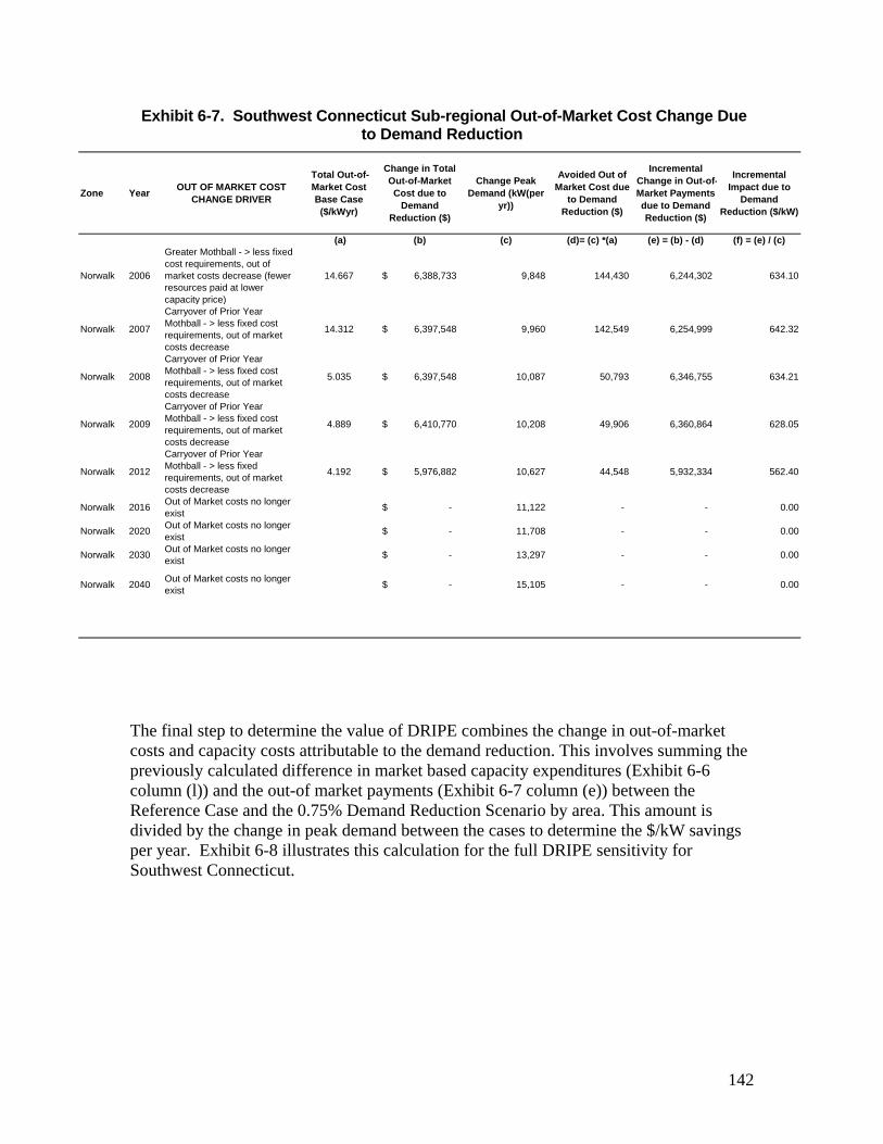
142
Zone Year OUT OF MARKET COST CHANGE DRIVER
Total Out-of-Market Cost Base Case
($/kWyr)
Change in Total Out-of-Market Cost due to
Demand Reduction ($)
Change Peak Demand (kW(per
yr))
Avoided Out of Market Cost due
to Demand Reduction ($)
Incremental Change in Out-of-Market Payments due to Demand Reduction ($)
Incremental Impact due to
Demand Reduction ($/kW)
(a) (b) (c) (d)= (c) *(a) (e) = (b) - (d) (f) = (e) / (c)
Norwalk 2006
Greater Mothball - > less fixed cost requirements, out of market costs decrease (fewer resources paid at lower capacity price)
14.667 $ 6,388,733 9,848 144,430 6,244,302 634.10
Norwalk 2007
Carryover of Prior Year Mothball - > less fixed cost requirements, out of market costs decrease
14.312 $ 6,397,548 9,960 142,549 6,254,999 642.32
Norwalk 2008
Carryover of Prior Year Mothball - > less fixed cost requirements, out of market costs decrease
5.035 $ 6,397,548 10,087 50,793 6,346,755 634.21
Norwalk 2009
Carryover of Prior Year Mothball - > less fixed cost requirements, out of market costs decrease
4.889 $ 6,410,770 10,208 49,906 6,360,864 628.05
Norwalk 2012
Carryover of Prior Year Mothball - > less fixed requirements, out of market costs decrease
4.192 $ 5,976,882 10,627 44,548 5,932,334 562.40
Norwalk 2016 Out of Market costs no longer exist $ - 11,122 - - 0.00
Norwalk 2020 Out of Market costs no longer exist $ - 11,708 - - 0.00
Norwalk 2030 Out of Market costs no longer exist $ - 13,297 - - 0.00
Norwalk 2040 Out of Market costs no longer exist $ - 15,105 - - 0.00
Exhibit 6-7. Southwest Connecticut Sub-regional Out-of-Market Cost Change Due to Demand Reduction
The final step to determine the value of DRIPE combines the change in out-of-market costs and capacity costs attributable to the demand reduction. This involves summing the previously calculated difference in market based capacity expenditures (Exhibit 6-6 column (l)) and the out-of market payments (Exhibit 6-7 column (e)) between the Reference Case and the 0.75% Demand Reduction Scenario by area. This amount is divided by the change in peak demand between the cases to determine the $/kW savings per year. Exhibit 6-8 illustrates this calculation for the full DRIPE sensitivity for Southwest Connecticut.
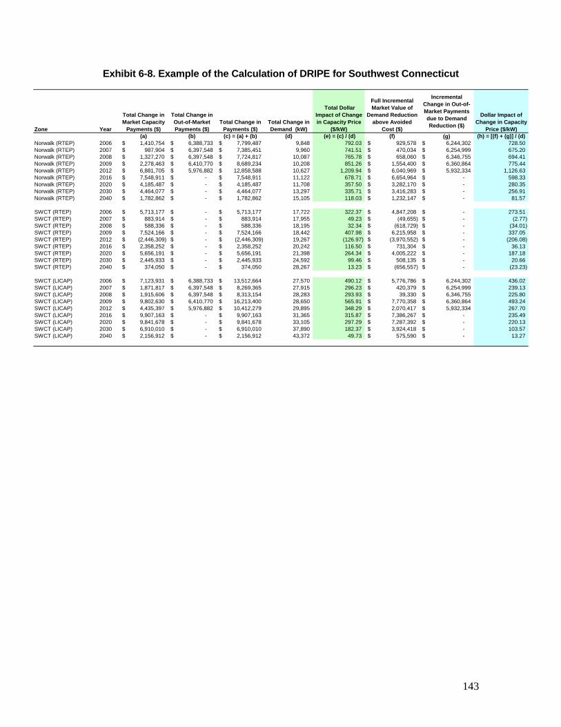
143
Exhibit 6-8. Example of the Calculation of DRIPE for Southwest Connecticut
Zone Year
Total Change in Market Capacity
Payments ($)
Total Change in Out-of-Market Payments ($)
Total Change in Payments ($)
Total Change in Demand (kW)
Total Dollar Impact of Change in Capacity Price
($/kW)
Full Incremental Market Value of
Demand Reduction above Avoided
Cost ($)
Incremental Change in Out-of-Market Payments due to Demand Reduction ($)
Dollar Impact of Change in Capacity
Price ($/kW)(a) (b) (c) = (a) + (b) (d) (e) = (c) / (d) (f) (g) (h) = [(f) + (g)] / (d)
Norwalk (RTEP) 2006 1,410,754$ 6,388,733$ 7,799,487$ 9,848 792.03 929,578$ 6,244,302$ 728.50 Norwalk (RTEP) 2007 987,904$ 6,397,548$ 7,385,451$ 9,960 741.51 470,034$ 6,254,999$ 675.20 Norwalk (RTEP) 2008 1,327,270$ 6,397,548$ 7,724,817$ 10,087 765.78 658,060$ 6,346,755$ 694.41 Norwalk (RTEP) 2009 2,278,463$ 6,410,770$ 8,689,234$ 10,208 851.26 1,554,400$ 6,360,864$ 775.44 Norwalk (RTEP) 2012 6,881,705$ 5,976,882$ 12,858,588$ 10,627 1,209.94 6,040,969$ 5,932,334$ 1,126.63 Norwalk (RTEP) 2016 7,548,911$ -$ 7,548,911$ 11,122 678.71 6,654,964$ -$ 598.33 Norwalk (RTEP) 2020 4,185,487$ -$ 4,185,487$ 11,708 357.50 3,282,170$ -$ 280.35 Norwalk (RTEP) 2030 4,464,077$ -$ 4,464,077$ 13,297 335.71 3,416,283$ -$ 256.91 Norwalk (RTEP) 2040 1,782,862$ -$ 1,782,862$ 15,105 118.03 1,232,147$ -$ 81.57
SWCT (RTEP) 2006 5,713,177$ -$ 5,713,177$ 17,722 322.37 4,847,208$ -$ 273.51 SWCT (RTEP) 2007 883,914$ -$ 883,914$ 17,955 49.23 (49,655)$ -$ (2.77) SWCT (RTEP) 2008 588,336$ -$ 588,336$ 18,195 32.34 (618,729)$ -$ (34.01) SWCT (RTEP) 2009 7,524,166$ -$ 7,524,166$ 18,442 407.98 6,215,958$ -$ 337.05 SWCT (RTEP) 2012 (2,446,309)$ -$ (2,446,309)$ 19,267 (126.97) (3,970,552)$ -$ (206.08) SWCT (RTEP) 2016 2,358,252$ -$ 2,358,252$ 20,242 116.50 731,304$ -$ 36.13 SWCT (RTEP) 2020 5,656,191$ -$ 5,656,191$ 21,398 264.34 4,005,222$ -$ 187.18 SWCT (RTEP) 2030 2,445,933$ -$ 2,445,933$ 24,592 99.46 508,135$ -$ 20.66 SWCT (RTEP) 2040 374,050$ -$ 374,050$ 28,267 13.23 (656,557)$ -$ (23.23)
SWCT (LICAP) 2006 7,123,931$ 6,388,733$ 13,512,664$ 27,570 490.12 5,776,786$ 6,244,302$ 436.02 SWCT (LICAP) 2007 1,871,817$ 6,397,548$ 8,269,365$ 27,915 296.23 420,379$ 6,254,999$ 239.13 SWCT (LICAP) 2008 1,915,606$ 6,397,548$ 8,313,154$ 28,283 293.93 39,330$ 6,346,755$ 225.80 SWCT (LICAP) 2009 9,802,630$ 6,410,770$ 16,213,400$ 28,650 565.91 7,770,358$ 6,360,864$ 493.24 SWCT (LICAP) 2012 4,435,397$ 5,976,882$ 10,412,279$ 29,895 348.29 2,070,417$ 5,932,334$ 267.70 SWCT (LICAP) 2016 9,907,163$ -$ 9,907,163$ 31,365 315.87 7,386,267$ -$ 235.49 SWCT (LICAP) 2020 9,841,678$ -$ 9,841,678$ 33,105 297.29 7,287,392$ -$ 220.13 SWCT (LICAP) 2030 6,910,010$ -$ 6,910,010$ 37,890 182.37 3,924,418$ -$ 103.57 SWCT (LICAP) 2040 2,156,912$ -$ 2,156,912$ 43,372 49.73 575,590$ -$ 13.27
The DRIPE Light analysis differs from the full DRIPE scenario in the assumption relating to participation in the spot market. DRIPE Light assumes that 10 percent of the market transacts at the spot value while the remainder of the market transacts at fixed bilateral contract prices. With the exception of the volumes, the methodology used to determine the DRIPE Light benefit is consistent with that used for Full DRIPE. Exhibit 6-9 combines the steps presented above to illustrate the DRIPE Light calculation. Here, the assumption is that the capacity under contract in the Base Case is equal to 10 percent of the total market clearing capacity under the LICAP curve in each year. It is further assumed that the sensitivity case does not affect the contracted capacity value. Hence the total quantity that participates in the spot market is equal to the total Sensitivity case supply minus the Base Case supply under contract where the Base Case supply under contract is equal to 90 percent of the total Base Case supply. Once the quantity participating in the spot market is determined, the total change in capacity expenses is calculates as the Base Case spot market payments less the Sensitivity Case spot market payments. As in the full DRIPE, the total change in out-of-market expenses is added to the total market change to determine the total benefit (column (l) in Exhibit 6-9). As in the full DRIPE, the avoided cost (demand reduction times capacity avoided cost from the Base Case) is then subtracted from the total benefit to determine the amount associated with the price and out-of market cost response. This is then divided by the demand reduction to determine a $/kW value.
144
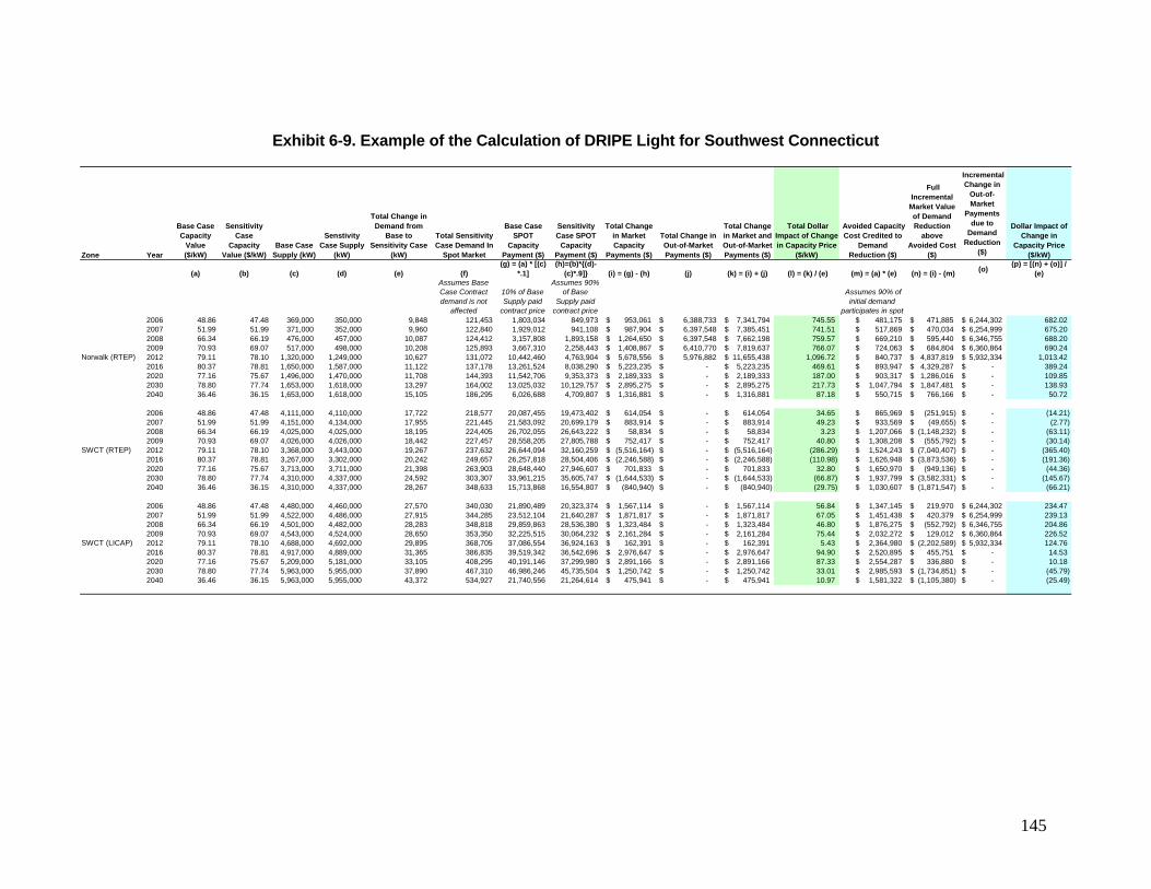
145
Exhibit 6-9. Example of the Calculation of DRIPE Light for Southwest Connecticut
Zone Year
Base Case Capacity
Value ($/kW)
Sensitivity Case
Capacity Value ($/kW)
Base Case Supply (kW)
Senstivity Case Supply
(kW)
Total Change in Demand from
Base to Sensitivity Case
(kW)
Total Sensitivity Case Demand In
Spot Market
Base Case SPOT
Capacity Payment ($)
Sensitivity Case SPOT
Capacity Payment ($)
Total Change in Market Capacity
Payments ($)
Total Change in Out-of-Market Payments ($)
Total Change in Market and Out-of-Market Payments ($)
Total Dollar Impact of Change in Capacity Price
($/kW)
Avoided Capacity Cost Credited to
Demand Reduction ($)
Full Incremental
Market Value of Demand Reduction
above Avoided Cost
($)
Incremental Change in
Out-of-Market
Payments due to
Demand Reduction
($)
Dollar Impact of Change in
Capacity Price ($/kW)
(a) (b) (c) (d) (e) (f)(g) = (a) * [(c)
*.1](h)=(b)*{(d)-
(c)*.9]} (i) = (g) - (h) (j) (k) = (i) + (j) (l) = (k) / (e) (m) = (a) * (e) (n) = (i) - (m) (o) (p) = [(n) + (o)] /
(e)Assumes Base Case Contract demand is not
affected
10% of Base Supply paid
contract price
Assumes 90% of Base
Supply paid contract price
Assumes 90% of initial demand
participates in spot 2006 48.86 47.48 369,000 350,000 9,848 121,453 1,803,034 849,973 953,061$ 6,388,733$ 7,341,794$ 745.55 481,175$ 471,885$ 6,244,302$ 682.02 2007 51.99 51.99 371,000 352,000 9,960 122,840 1,929,012 941,108 987,904$ 6,397,548$ 7,385,451$ 741.51 517,869$ 470,034$ 6,254,999$ 675.20 2008 66.34 66.19 476,000 457,000 10,087 124,412 3,157,808 1,893,158 1,264,650$ 6,397,548$ 7,662,198$ 759.57 669,210$ 595,440$ 6,346,755$ 688.20 2009 70.93 69.07 517,000 498,000 10,208 125,893 3,667,310 2,258,443 1,408,867$ 6,410,770$ 7,819,637$ 766.07 724,063$ 684,804$ 6,360,864$ 690.24 2012 79.11 78.10 1,320,000 1,249,000 10,627 131,072 10,442,460 4,763,904 5,678,556$ 5,976,882$ 11,655,438$ 1,096.72 840,737$ 4,837,819$ 5,932,334$ 1,013.42 2016 80.37 78.81 1,650,000 1,587,000 11,122 137,178 13,261,524 8,038,290 5,223,235$ -$ 5,223,235$ 469.61 893,947$ 4,329,287$ -$ 389.24 2020 77.16 75.67 1,496,000 1,470,000 11,708 144,393 11,542,706 9,353,373 2,189,333$ -$ 2,189,333$ 187.00 903,317$ 1,286,016$ -$ 109.85 2030 78.80 77.74 1,653,000 1,618,000 13,297 164,002 13,025,032 10,129,757 2,895,275$ -$ 2,895,275$ 217.73 1,047,794$ 1,847,481$ -$ 138.93 2040 36.46 36.15 1,653,000 1,618,000 15,105 186,295 6,026,688 4,709,807 1,316,881$ -$ 1,316,881$ 87.18 550,715$ 766,166$ -$ 50.72
2006 48.86 47.48 4,111,000 4,110,000 17,722 218,577 20,087,455 19,473,402 614,054$ -$ 614,054$ 34.65 865,969$ (251,915)$ -$ (14.21) 2007 51.99 51.99 4,151,000 4,134,000 17,955 221,445 21,583,092 20,699,179 883,914$ -$ 883,914$ 49.23 933,569$ (49,655)$ -$ (2.77) 2008 66.34 66.19 4,025,000 4,025,000 18,195 224,405 26,702,055 26,643,222 58,834$ -$ 58,834$ 3.23 1,207,066$ (1,148,232)$ -$ (63.11) 2009 70.93 69.07 4,026,000 4,026,000 18,442 227,457 28,558,205 27,805,788 752,417$ -$ 752,417$ 40.80 1,308,208$ (555,792)$ -$ (30.14) 2012 79.11 78.10 3,368,000 3,443,000 19,267 237,632 26,644,094 32,160,259 (5,516,164)$ -$ (5,516,164)$ (286.29) 1,524,243$ (7,040,407)$ -$ (365.40) 2016 80.37 78.81 3,267,000 3,302,000 20,242 249,657 26,257,818 28,504,406 (2,246,588)$ -$ (2,246,588)$ (110.98) 1,626,948$ (3,873,536)$ -$ (191.36) 2020 77.16 75.67 3,713,000 3,711,000 21,398 263,903 28,648,440 27,946,607 701,833$ -$ 701,833$ 32.80 1,650,970$ (949,136)$ -$ (44.36) 2030 78.80 77.74 4,310,000 4,337,000 24,592 303,307 33,961,215 35,605,747 (1,644,533)$ -$ (1,644,533)$ (66.87) 1,937,799$ (3,582,331)$ -$ (145.67) 2040 36.46 36.15 4,310,000 4,337,000 28,267 348,633 15,713,868 16,554,807 (840,940)$ -$ (840,940)$ (29.75) 1,030,607$ (1,871,547)$ -$ (66.21)
2006 48.86 47.48 4,480,000 4,460,000 27,570 340,030 21,890,489 20,323,374 1,567,114$ -$ 1,567,114$ 56.84 1,347,145$ 219,970$ 6,244,302$ 234.47 2007 51.99 51.99 4,522,000 4,486,000 27,915 344,285 23,512,104 21,640,287 1,871,817$ -$ 1,871,817$ 67.05 1,451,438$ 420,379$ 6,254,999$ 239.13 2008 66.34 66.19 4,501,000 4,482,000 28,283 348,818 29,859,863 28,536,380 1,323,484$ -$ 1,323,484$ 46.80 1,876,275$ (552,792)$ 6,346,755$ 204.86 2009 70.93 69.07 4,543,000 4,524,000 28,650 353,350 32,225,515 30,064,232 2,161,284$ -$ 2,161,284$ 75.44 2,032,272$ 129,012$ 6,360,864$ 226.52 2012 79.11 78.10 4,688,000 4,692,000 29,895 368,705 37,086,554 36,924,163 162,391$ -$ 162,391$ 5.43 2,364,980$ (2,202,589)$ 5,932,334$ 124.76 2016 80.37 78.81 4,917,000 4,889,000 31,365 386,835 39,519,342 36,542,696 2,976,647$ -$ 2,976,647$ 94.90 2,520,895$ 455,751$ -$ 14.53 2020 77.16 75.67 5,209,000 5,181,000 33,105 408,295 40,191,146 37,299,980 2,891,166$ -$ 2,891,166$ 87.33 2,554,287$ 336,880$ -$ 10.18 2030 78.80 77.74 5,963,000 5,955,000 37,890 467,310 46,986,246 45,735,504 1,250,742$ -$ 1,250,742$ 33.01 2,985,593$ (1,734,851)$ -$ (45.79) 2040 36.46 36.15 5,963,000 5,955,000 43,372 534,927 21,740,556 21,264,614 475,941$ -$ 475,941$ 10.97 1,581,322$ (1,105,380)$ -$ (25.49)
SWCT (LICAP)
SWCT (RTEP)
Norwalk (RTEP)
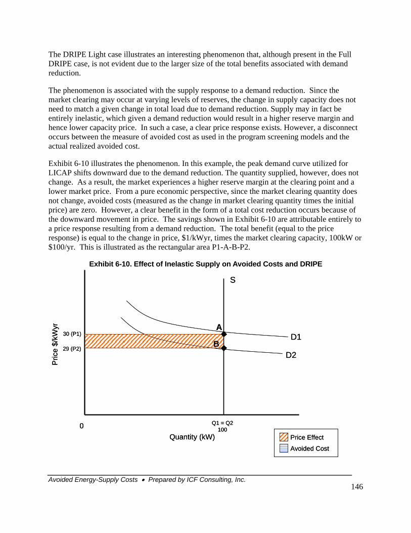
Avoided Energy-Supply Costs • Prepared by ICF Consulting, Inc.
146
The DRIPE Light case illustrates an interesting phenomenon that, although present in the Full DRIPE case, is not evident due to the larger size of the total benefits associated with demand reduction.
The phenomenon is associated with the supply response to a demand reduction. Since the market clearing may occur at varying levels of reserves, the change in supply capacity does not need to match a given change in total load due to demand reduction. Supply may in fact be entirely inelastic, which given a demand reduction would result in a higher reserve margin and hence lower capacity price. In such a case, a clear price response exists. However, a disconnect occurs between the measure of avoided cost as used in the program screening models and the actual realized avoided cost.
Exhibit 6-10 illustrates the phenomenon. In this example, the peak demand curve utilized for LICAP shifts downward due to the demand reduction. The quantity supplied, however, does not change. As a result, the market experiences a higher reserve margin at the clearing point and a lower market price. From a pure economic perspective, since the market clearing quantity does not change, avoided costs (measured as the change in market clearing quantity times the initial price) are zero. However, a clear benefit in the form of a total cost reduction occurs because of the downward movement in price. The savings shown in Exhibit 6-10 are attributable entirely to a price response resulting from a demand reduction. The total benefit (equal to the price response) is equal to the change in price, $1/kWyr, times the market clearing capacity, 100kW or $100/yr. This is illustrated as the rectangular area P1-A-B-P2.
Exhibit 6-10. Effect of Inelastic Supply on Avoided Costs and DRIPE
Pric
e $/
kWyr
Quantity (kW)
Q1 = Q2100
30 (P1)
29 (P2)
0
S
D1
D2B
Price Effect
Avoided Cost
A
Pric
e $/
kWyr
Quantity (kW)
Q1 = Q2100
30 (P1)
29 (P2)
0
S
D1
D2B
Price Effect
Avoided Cost
A
Avoided Energy-Supply Costs • Prepared by ICF Consulting, Inc.
147
Since the supply response and hence the change in the market clearing quantity can not be known in advance, to measure the avoided costs the AESC screening tools utilize the load savings achieved through the demand reduction program. Avoided costs are calculated as the change in peak demand (associated with the energy efficiency program) times the initial price. In the earlier example, the demand reduction of 10kW (see Exhibit 6-1) times the initial price of $30/kWyr would produce an avoided cost of $300/yr.
In contrast, the total benefit is $100/yr, resulting in an overstatement of avoided costs by $200/yr. Since total savings in the DRIPE Light case are significantly below that in the DRIPE case, the potential for such an overstatement to occur increases. Such instances are indicated in the DRIPE Light results when the incremental DRIPE value becomes negative.
A real life illustration of this is seen in the SWCT RTEP zone 2008 DRIPE and DRIPE LIGHT incremental savings shown in Exhibits 6-8 and 6-9 respectively. In the full DRIPE scenario, the total savings in market capacity payments are $7.5 million. In the DRIPE Light scenario, when only 10 percent of the capacity is assumed to transact in the spot market, the total savings are reduced to one tenth of this value at $752,417. Although the market clearing quantity is unchanged between the Reference Case and 0.75% Peak Demand Reduction scenario, the avoided costs calculated in the screening tools would consider avoided costs equal to the 18 MW of demand reduction times the marginal capacity value of $70.93/kWyr or $1.3 million. Since the full DRIPE savings are well above the avoided cost calculated based on the demand reduction, the incremental DRIPE value appears reasonable at $337.05/kW for the year. However, the calculated avoided costs are nearly double the total benefit associated with DRIPE Light. Based on the approach described in the methodology section, the incremental DRIPE Light will compensate for this overstatement by setting the increment DRIPE Light value equal to the amount that was over credited in the avoided cost calculation. Hence the DRIPE Light for SWCT becomes -$30.14/kW in 2009.
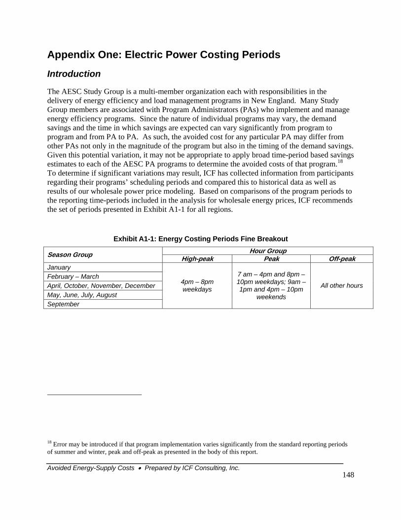
Avoided Energy-Supply Costs • Prepared by ICF Consulting, Inc.
148
Appendix One: Electric Power Costing Periods
Introduction
The AESC Study Group is a multi-member organization each with responsibilities in the delivery of energy efficiency and load management programs in New England. Many Study Group members are associated with Program Administrators (PAs) who implement and manage energy efficiency programs. Since the nature of individual programs may vary, the demand savings and the time in which savings are expected can vary significantly from program to program and from PA to PA. As such, the avoided cost for any particular PA may differ from other PAs not only in the magnitude of the program but also in the timing of the demand savings. Given this potential variation, it may not be appropriate to apply broad time-period based savings estimates to each of the AESC PA programs to determine the avoided costs of that program.18 To determine if significant variations may result, ICF has collected information from participants regarding their programs’ scheduling periods and compared this to historical data as well as results of our wholesale power price modeling. Based on comparisons of the program periods to the reporting time-periods included in the analysis for wholesale energy prices, ICF recommends the set of periods presented in Exhibit A1-1 for all regions.
Exhibit A1-1: Energy Costing Periods Fine Breakout
Hour Group Season Group High-peak Peak Off-peak January February – March April, October, November, December May, June, July, August September
4pm – 8pm weekdays
7 am – 4pm and 8pm – 10pm weekdays; 9am – 1pm and 4pm – 10pm
weekends
All other hours
18 Error may be introduced if that program implementation varies significantly from the standard reporting periods of summer and winter, peak and off-peak as presented in the body of this report.
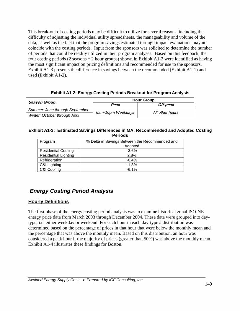
Avoided Energy-Supply Costs • Prepared by ICF Consulting, Inc.
149
This break-out of costing periods may be difficult to utilize for several reasons, including the difficulty of adjusting the individual utility spreadsheets, the manageability and volume of the data, as well as the fact that the program savings estimated through impact evaluations may not coincide with the costing periods. Input from the sponsors was solicited to determine the number of periods that could be readily utilized in their program analyses. Based on this feedback, the four costing periods (2 seasons * 2 hour groups) shown in Exhibit A1-2 were identified as having the most significant impact on pricing definitions and recommended for use to the sponsors. Exhibit A1-3 presents the difference in savings between the recommended (Exhibit A1-1) and used (Exhibit A1-2).
Exhibit A1-2: Energy Costing Periods Breakout for Program Analysis
Hour Group Season Group Peak Off-peak Summer: June through September Winter: October through April
6am-10pm Weekdays All other hours
Exhibit A1-3: Estimated Savings Differences in MA: Recommended and Adopted Costing Periods
Program % Delta in Savings Between the Recommended and Adopted
Residential Cooling -3.6% Residential Lighting 2.8% Refrigeration -0.4% C&I Lighting -1.8% C&I Cooling -6.1%
Energy Costing Period Analysis
Hourly Definitions
The first phase of the energy costing period analysis was to examine historical zonal ISO-NE energy price data from March 2003 through December 2004. These data were grouped into day-type, i.e. either weekday or weekend. For each hour in each day-type a distribution was determined based on the percentage of prices in that hour that were below the monthly mean and the percentage that was above the monthly mean. Based on this distribution, an hour was considered a peak hour if the majority of prices (greater than 50%) was above the monthly mean. Exhibit A1-4 illustrates these findings for Boston.
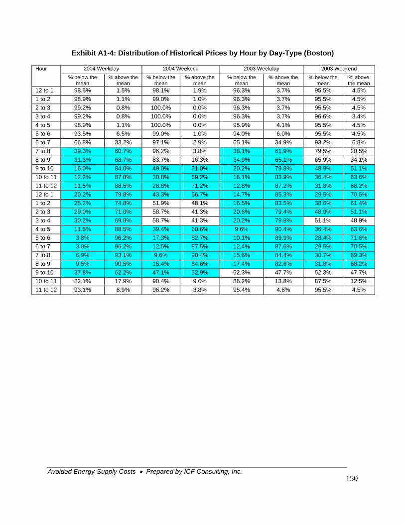
Avoided Energy-Supply Costs • Prepared by ICF Consulting, Inc.
150
Exhibit A1-4: Distribution of Historical Prices by Hour by Day-Type (Boston)
Hour 2004 Weekday 2004 Weekend 2003 Weekday 2003 Weekend % below the
mean % above the
mean % below the
mean % above the
mean % below the
mean % above the
mean % below the
mean % above the mean
12 to 1 98.5% 1.5% 98.1% 1.9% 96.3% 3.7% 95.5% 4.5% 1 to 2 98.9% 1.1% 99.0% 1.0% 96.3% 3.7% 95.5% 4.5% 2 to 3 99.2% 0.8% 100.0% 0.0% 96.3% 3.7% 95.5% 4.5% 3 to 4 99.2% 0.8% 100.0% 0.0% 96.3% 3.7% 96.6% 3.4% 4 to 5 98.9% 1.1% 100.0% 0.0% 95.9% 4.1% 95.5% 4.5% 5 to 6 93.5% 6.5% 99.0% 1.0% 94.0% 6.0% 95.5% 4.5% 6 to 7 66.8% 33.2% 97.1% 2.9% 65.1% 34.9% 93.2% 6.8% 7 to 8 39.3% 60.7% 96.2% 3.8% 38.1% 61.9% 79.5% 20.5% 8 to 9 31.3% 68.7% 83.7% 16.3% 34.9% 65.1% 65.9% 34.1% 9 to 10 16.0% 84.0% 49.0% 51.0% 20.2% 79.8% 48.9% 51.1% 10 to 11 12.2% 87.8% 30.8% 69.2% 16.1% 83.9% 36.4% 63.6% 11 to 12 11.5% 88.5% 28.8% 71.2% 12.8% 87.2% 31.8% 68.2% 12 to 1 20.2% 79.8% 43.3% 56.7% 14.7% 85.3% 29.5% 70.5% 1 to 2 25.2% 74.8% 51.9% 48.1% 16.5% 83.5% 38.6% 61.4% 2 to 3 29.0% 71.0% 58.7% 41.3% 20.6% 79.4% 48.9% 51.1% 3 to 4 30.2% 69.8% 58.7% 41.3% 20.2% 79.8% 51.1% 48.9% 4 to 5 11.5% 88.5% 39.4% 60.6% 9.6% 90.4% 36.4% 63.6% 5 to 6 3.8% 96.2% 17.3% 82.7% 10.1% 89.9% 28.4% 71.6% 6 to 7 3.8% 96.2% 12.5% 87.5% 12.4% 87.6% 29.5% 70.5% 7 to 8 6.9% 93.1% 9.6% 90.4% 15.6% 84.4% 30.7% 69.3% 8 to 9 9.5% 90.5% 15.4% 84.6% 17.4% 82.6% 31.8% 68.2% 9 to 10 37.8% 62.2% 47.1% 52.9% 52.3% 47.7% 52.3% 47.7% 10 to 11 82.1% 17.9% 90.4% 9.6% 86.2% 13.8% 87.5% 12.5% 11 to 12 93.1% 6.9% 96.2% 3.8% 95.4% 4.6% 95.5% 4.5%
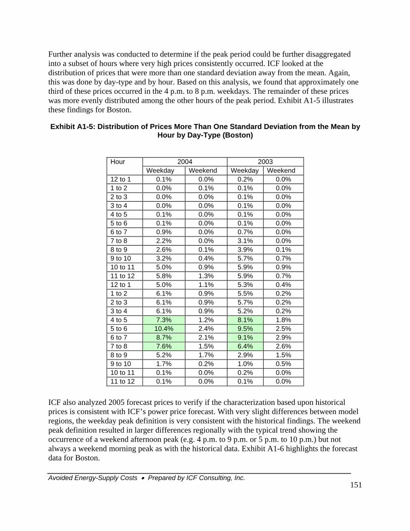
Avoided Energy-Supply Costs • Prepared by ICF Consulting, Inc.
151
Further analysis was conducted to determine if the peak period could be further disaggregated into a subset of hours where very high prices consistently occurred. ICF looked at the distribution of prices that were more than one standard deviation away from the mean. Again, this was done by day-type and by hour. Based on this analysis, we found that approximately one third of these prices occurred in the 4 p.m. to 8 p.m. weekdays. The remainder of these prices was more evenly distributed among the other hours of the peak period. Exhibit A1-5 illustrates these findings for Boston.
Exhibit A1-5: Distribution of Prices More Than One Standard Deviation from the Mean by Hour by Day-Type (Boston)
ICF also analyzed 2005 forecast prices to verify if the characterization based upon historical prices is consistent with ICF’s power price forecast. With very slight differences between model regions, the weekday peak definition is very consistent with the historical findings. The weekend peak definition resulted in larger differences regionally with the typical trend showing the occurrence of a weekend afternoon peak (e.g. 4 p.m. to 9 p.m. or 5 p.m. to 10 p.m.) but not always a weekend morning peak as with the historical data. Exhibit A1-6 highlights the forecast data for Boston.
Hour 2004 2003 Weekday Weekend Weekday Weekend 12 to 1 0.1% 0.0% 0.2% 0.0% 1 to 2 0.0% 0.1% 0.1% 0.0% 2 to 3 0.0% 0.0% 0.1% 0.0% 3 to 4 0.0% 0.0% 0.1% 0.0% 4 to 5 0.1% 0.0% 0.1% 0.0% 5 to 6 0.1% 0.0% 0.1% 0.0% 6 to 7 0.9% 0.0% 0.7% 0.0% 7 to 8 2.2% 0.0% 3.1% 0.0% 8 to 9 2.6% 0.1% 3.9% 0.1% 9 to 10 3.2% 0.4% 5.7% 0.7% 10 to 11 5.0% 0.9% 5.9% 0.9% 11 to 12 5.8% 1.3% 5.9% 0.7% 12 to 1 5.0% 1.1% 5.3% 0.4% 1 to 2 6.1% 0.9% 5.5% 0.2% 2 to 3 6.1% 0.9% 5.7% 0.2% 3 to 4 6.1% 0.9% 5.2% 0.2% 4 to 5 7.3% 1.2% 8.1% 1.8% 5 to 6 10.4% 2.4% 9.5% 2.5% 6 to 7 8.7% 2.1% 9.1% 2.9% 7 to 8 7.6% 1.5% 6.4% 2.6% 8 to 9 5.2% 1.7% 2.9% 1.5% 9 to 10 1.7% 0.2% 1.0% 0.5% 10 to 11 0.1% 0.0% 0.2% 0.0% 11 to 12 0.1% 0.0% 0.1% 0.0%
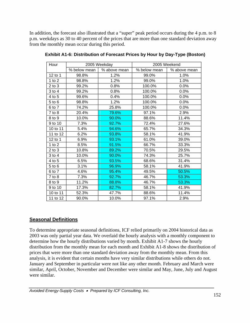
Avoided Energy-Supply Costs • Prepared by ICF Consulting, Inc.
152
In addition, the forecast also illustrated that a “super” peak period occurs during the 4 p.m. to 8 p.m. weekdays as 30 to 40 percent of the prices that are more than one standard deviation away from the monthly mean occur during this period.
Exhibit A1-6: Distribution of Forecast Prices by Hour by Day-Type (Boston)
Hour 2005 Weekday 2005 Weekend % below mean % above mean % below mean % above mean 12 to 1 98.8% 1.2% 99.0% 1.0% 1 to 2 98.8% 1.2% 99.0% 1.0% 2 to 3 99.2% 0.8% 100.0% 0.0% 3 to 4 99.2% 0.8% 100.0% 0.0% 4 to 5 99.6% 0.4% 100.0% 0.0% 5 to 6 98.8% 1.2% 100.0% 0.0% 6 to 7 74.2% 25.8% 100.0% 0.0% 7 to 8 20.4% 79.6% 97.1% 2.9% 8 to 9 10.0% 90.0% 88.6% 11.4% 9 to 10 7.3% 92.7% 72.4% 27.6% 10 to 11 5.4% 94.6% 65.7% 34.3% 11 to 12 6.2% 93.8% 58.1% 41.9% 12 to 1 6.9% 93.1% 61.0% 39.0% 1 to 2 8.5% 91.5% 66.7% 33.3% 2 to 3 10.8% 89.2% 70.5% 29.5% 3 to 4 10.0% 90.0% 74.3% 25.7% 4 to 5 6.5% 93.5% 68.6% 31.4% 5 to 6 3.1% 96.9% 58.1% 41.9% 6 to 7 4.6% 95.4% 49.5% 50.5% 7 to 8 7.3% 92.7% 46.7% 53.3% 8 to 9 11.2% 88.8% 46.7% 53.3% 9 to 10 17.3% 82.7% 58.1% 41.9% 10 to 11 52.3% 47.7% 88.6% 11.4% 11 to 12 90.0% 10.0% 97.1% 2.9%
Seasonal Definitions
To determine appropriate seasonal definitions, ICF relied primarily on 2004 historical data as 2003 was only partial year data. We overlaid the hourly analysis with a monthly component to determine how the hourly distributions varied by month. Exhibit A1-7 shows the hourly distribution from the monthly mean for each month and Exhibit A1-8 shows the distribution of prices that were more than one standard deviation away from the monthly mean. From this analysis, it is evident that certain months have very similar distributions while others do not. January and September in particular were not like any other month. February and March were similar, April, October, November and December were similar and May, June, July and August were similar.
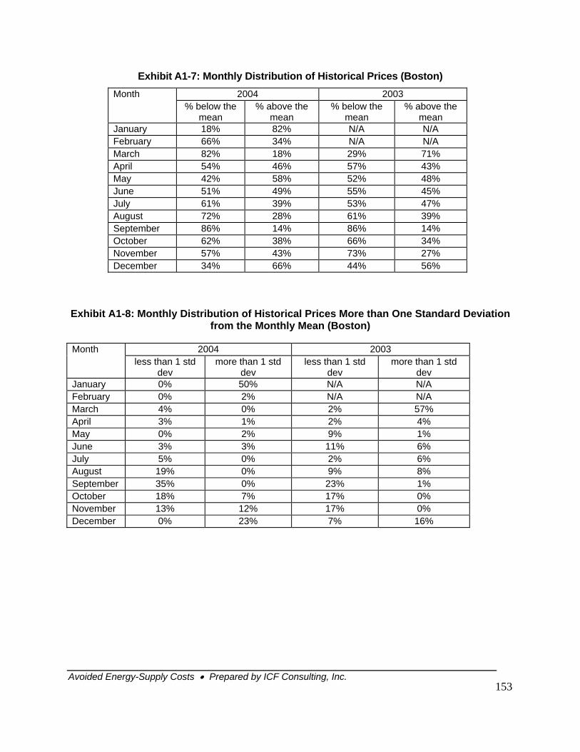
Avoided Energy-Supply Costs • Prepared by ICF Consulting, Inc.
153
Exhibit A1-7: Monthly Distribution of Historical Prices (Boston) Month 2004 2003 % below the
mean % above the
mean % below the
mean % above the
mean January 18% 82% N/A N/A February 66% 34% N/A N/A March 82% 18% 29% 71% April 54% 46% 57% 43% May 42% 58% 52% 48% June 51% 49% 55% 45% July 61% 39% 53% 47% August 72% 28% 61% 39% September 86% 14% 86% 14% October 62% 38% 66% 34% November 57% 43% 73% 27% December 34% 66% 44% 56%
Exhibit A1-8: Monthly Distribution of Historical Prices More than One Standard Deviation from the Monthly Mean (Boston)
Month 2004 2003 less than 1 std
dev more than 1 std
dev less than 1 std
dev more than 1 std
dev January 0% 50% N/A N/A February 0% 2% N/A N/A March 4% 0% 2% 57% April 3% 1% 2% 4% May 0% 2% 9% 1% June 3% 3% 11% 6% July 5% 0% 2% 6% August 19% 0% 9% 8% September 35% 0% 23% 1% October 18% 7% 17% 0% November 13% 12% 17% 0% December 0% 23% 7% 16%
Avoided Energy-Supply Costs • Prepared by ICF Consulting, Inc.
154
Capacity Value Period Analysis
The Locational ICAP market is a monthly market - prices for capacity in New England are expected to vary from month to month based on the supply and demand conditions for that month. Although prices may vary by month, the bulk of the value associated with capacity is expected to be determined by the summer peak conditions consistent with the determination of the objective capability (OC)19 level. In other words, avoided capacity costs depend on the capability to reduce summer peak load. Regardless of whether prices vary monthly, the load reduction at peak will reduce the total cost of supply.
The rationale for the costing periods is that required investment in capacity will be reduced as a function of peak load reduction and LR regardless of price fluctuations.
Given this design in the LICAP curves, there are effectively two ways to impact capacity prices. First, shifts in the demand curve based on shifts in the OC from year to year will fundamentally alter the clearing prices in each month of the following year. This effect is independent of the direct avoided costs estimates and is reflected in the DRIPE analysis20. Second, shifts in the monthly supply curve or the quantity supplied will affect the monthly price. The supply driven changes (and their impact on the market clearing quantity and price) are also captured in the DRIPE analysis. Other variations may exist and affect the monthly markets; however, these two are the key drivers which can be directly impacted by demand reductions.
19 Objective Capability is the ISO term. This is also sometimes referred to as the locational installed capacity requirement.
20 See Chapter Six for discussion of DRIPE.
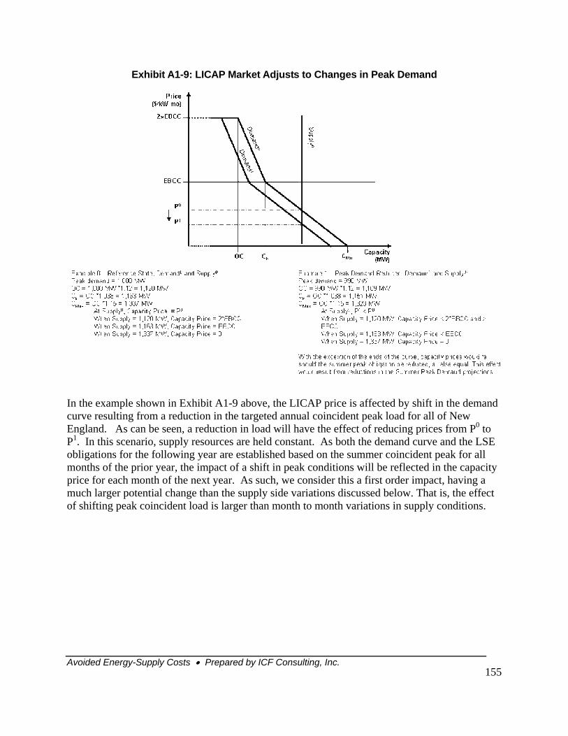
Avoided Energy-Supply Costs • Prepared by ICF Consulting, Inc.
155
Exhibit A1-9: LICAP Market Adjusts to Changes in Peak Demand
In the example shown in Exhibit A1-9 above, the LICAP price is affected by shift in the demand curve resulting from a reduction in the targeted annual coincident peak load for all of New England. As can be seen, a reduction in load will have the effect of reducing prices from P0 to P1. In this scenario, supply resources are held constant. As both the demand curve and the LSE obligations for the following year are established based on the summer coincident peak for all months of the prior year, the impact of a shift in peak conditions will be reflected in the capacity price for each month of the next year. As such, we consider this a first order impact, having a much larger potential change than the supply side variations discussed below. That is, the effect of shifting peak coincident load is larger than month to month variations in supply conditions.
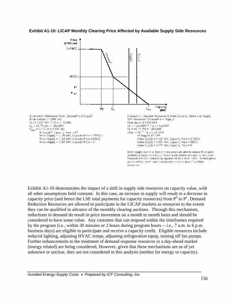
Avoided Energy-Supply Costs • Prepared by ICF Consulting, Inc.
156
Exhibit A1-10: LICAP Monthly Clearing Price Affected by Available Supply Side Resources
Exhibit A1-10 demonstrates the impact of a shift in supply side resources on capacity value, with all other assumptions held constant. In this case, an increase in supply will result in a decrease in capacity price (and hence the LSE total payments for capacity resources) from P0 to P1. Demand Reduction Resources are allowed to participate in the LICAP markets as resources to the extent they can be qualified in advance of the monthly clearing auctions. Through this mechanism, reductions in demand do result in price movement on a month to month basis and should be considered to have some value. Any customer that can respond within the timeframes required by the program (i.e., within 30 minutes or 2 hours during program hours -- i.e., 7 a.m. to 6 p.m. business days) are eligible to participate and receive a capacity credit. Eligible resources include reduced lighting, adjusting HVAC temps, adjusting refrigeration equip, turning off fan pumps. Further enhancements to the treatment of demand response resources in a day-ahead market (energy related) are being considered, However, given that these mechanisms are as of yet unknown or unclear, they are not considered in this analysis (neither for energy or capacity).
Avoided Energy-Supply Costs • Prepared by ICF Consulting, Inc.
157
Given the design of the New England LICAP markets, the majority of capacity value will be recognized based on summer coincident peak conditions. However, value will still be recognized for load reductions in non-coincident peak hours. For example demand response resources may have value in non-peak periods. ICF recommends the use of two costing periods for capacity, 1) Summer Peak, for use in evaluating energy efficiency measures that may impact the summer peak; and 2) all else, for use in evaluating Load Response measures that may be effective at reducing demand in non-peak periods. Further discussion on the application of Summer Peak Energy Efficiency and Load Response values is found in Appendix 2.
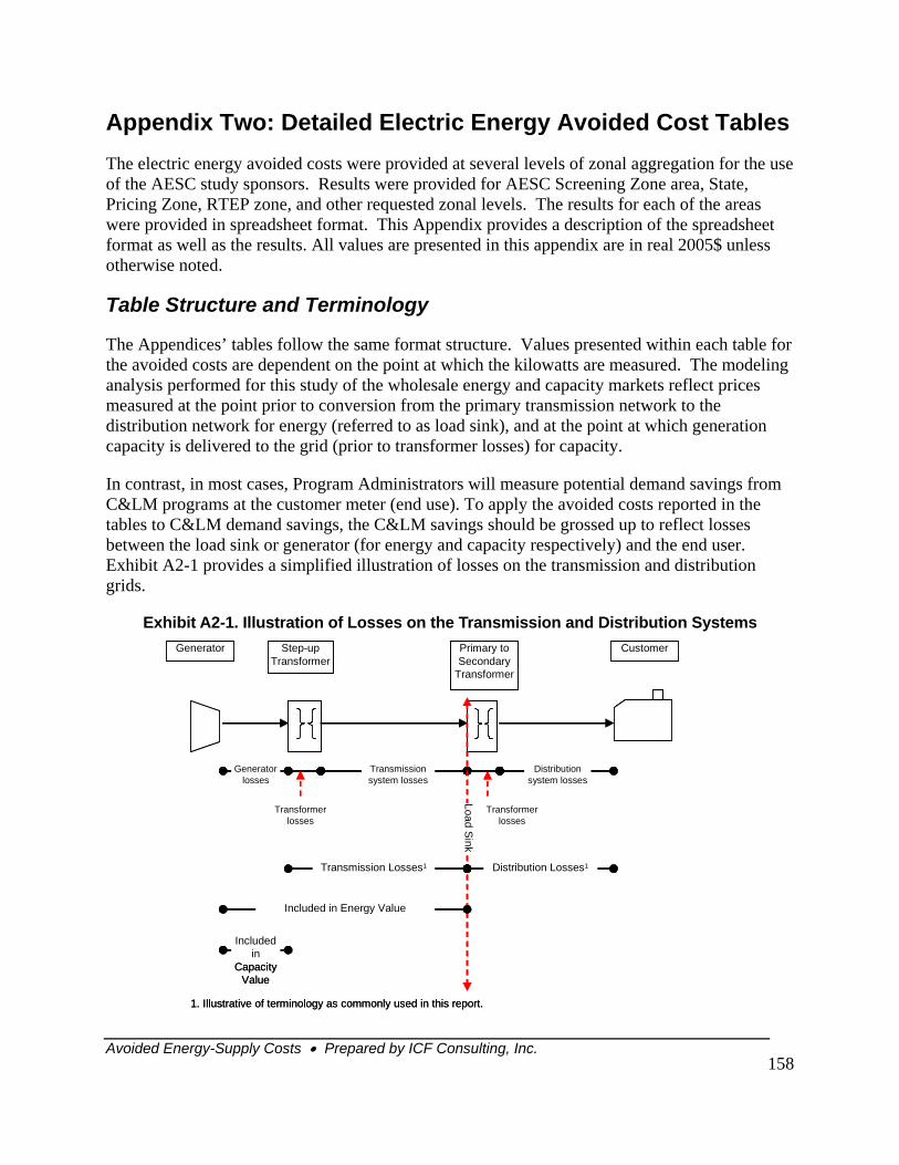
Avoided Energy-Supply Costs • Prepared by ICF Consulting, Inc.
158
Appendix Two: Detailed Electric Energy Avoided Cost Tables The electric energy avoided costs were provided at several levels of zonal aggregation for the use of the AESC study sponsors. Results were provided for AESC Screening Zone area, State, Pricing Zone, RTEP zone, and other requested zonal levels. The results for each of the areas were provided in spreadsheet format. This Appendix provides a description of the spreadsheet format as well as the results. All values are presented in this appendix are in real 2005$ unless otherwise noted.
Table Structure and Terminology
The Appendices’ tables follow the same format structure. Values presented within each table for the avoided costs are dependent on the point at which the kilowatts are measured. The modeling analysis performed for this study of the wholesale energy and capacity markets reflect prices measured at the point prior to conversion from the primary transmission network to the distribution network for energy (referred to as load sink), and at the point at which generation capacity is delivered to the grid (prior to transformer losses) for capacity.
In contrast, in most cases, Program Administrators will measure potential demand savings from C&LM programs at the customer meter (end use). To apply the avoided costs reported in the tables to C&LM demand savings, the C&LM savings should be grossed up to reflect losses between the load sink or generator (for energy and capacity respectively) and the end user. Exhibit A2-1 provides a simplified illustration of losses on the transmission and distribution grids.
Exhibit A2-1. Illustration of Losses on the Transmission and Distribution Systems Primary to Secondary
Transformer
Generator Step-up Transformer
Customer
Transformer losses
Transformer losses
Included in Energy Value
Transmission system losses
Generator losses
Distribution system losses
Load Sink
Included in
Capacity Value
Distribution Losses1Transmission Losses1
1. Illustrative of terminology as commonly used in this report.
Primary to Secondary
Transformer
Generator Step-up Transformer
Customer
Transformer losses
Transformer losses
Included in Energy Value
Transmission system losses
Generator losses
Distribution system losses
Load Sink
Included in
Capacity Value
Distribution Losses1Transmission Losses1
1. Illustrative of terminology as commonly used in this report.
Avoided Energy-Supply Costs • Prepared by ICF Consulting, Inc.
159
Total distribution losses as used herein indicate the losses that occur between the point of transmission voltage step-down to distribution voltage (including transformer losses) to the point of customer delivery. The forecast results presented in this report do not include distribution losses. A discussion on the estimation of losses consistent with the avoided costs is included in Chapter 3
Transmission losses as used herein reflect losses that occur from the point of generation power voltage step-up to transmission level voltage (including transformer losses), to the point of delivery to the load sink. Transmission losses are included in the energy forecasts provided herein (energy price forecasts are presented at the load sink); however, such losses are not included in the capacity forecasts.
Generator losses capture losses that occur between the generator and the step-up transformer to the transmission grid. Generator losses are included in both the energy and capacity forecasts (capacity price forecasts are provided at the generator level including generator losses).
The fields included are defined below in order of their appearance in the tables.
Winter Peak Energy ($/kWh): Values are avoided energy costs at the load sink. This represents the marginal cost of energy in the winter period peak hours defined as January, February, March, April, May, October, November and December, Monday through Friday 6am - 10pm (the 16 hour block beginning at 6am and ending at 9:59pm). To apply these values to CL&M savings measured at the customer meter, the savings should be grossed up for losses to the load sink level. To gross up kilowatt-hours savings measured at the customer meter, multiply the quantity (kWh) by the quantity one plus the distribution loss.
Winter Off-Peak Energy ($/kWh): Values are avoided energy costs at the load sink. This represents the marginal cost of energy in the winter period off-peak hours defined as January, February, March, April, May, October, November and December, 10:00pm – 5:59am Monday through Friday, and all day on Saturday and Sunday. When applying these values to C&LM savings measured at the customer meter, the savings should be grossed up for losses to the load sink level. To gross up kilowatt-hours savings measured at the customer meter, multiply the quantity (kWh) by the quantity one plus the distribution loss.
Summer Peak Energy ($/kWh): Values are avoided energy costs at the load sink. This represents the marginal cost of energy in the summer period peak hours defined as June, July, August and September, Monday through Friday 6:00am – 9:59pm. When applying these values to C&LM savings measured at the customer meter, the savings should be grossed up for losses to the load sink level. To gross up kilowatt-hours savings measured at the customer meter, multiply the quantity (kWh) by the quantity one plus the distribution loss.
Summer Off-Peak Energy ($/kWh): Values are avoided energy costs at the generator level. This represents the marginal cost of energy in the summer period off-peak hours defined as June, July, August and September, 10:00pm – 5:59am Monday through Friday, and all day Saturday and Sunday. When applying these values to C&LM savings measured at the customer meter, the savings should be grossed up for losses to the load sink level. To gross up kilowatt-hours savings
Avoided Energy-Supply Costs • Prepared by ICF Consulting, Inc.
160
measured at the customer meter, multiply the quantity (kWh) by the quantity one plus the distribution loss.
Annual Market Capacity Value ($/kW-yr): Reflects capacity price resulting from LICAP demand curve structure as modeled (beginning in 2006). The LICAP price is set by the LICAP demand curve and the capability bid into the market by each generator where generator losses are accounted for in the generator capability as modeled. This field provides the model results for capacity clearing value and does not include any incremental payments for out-of-market costs. The capacity price is measured at the generator level including generator losses. This value reflects the capacity value at summer coincident peak which is most likely to occur in the months of June, July or August between the hours of 3-5pm on a weekday21. In order to properly reflect the capacity avoided costs associated with LICAP purchases in the program screening tools, one should increase the megawatts as measured at the customer meter by the sum of the transmission and distribution losses. In addition, since each load serving entity has a target reserve margin above their peak obligation, the avoided megawatts (savings measured on the customer meter (MW) * [1 + (transmission loss (%) + distribution loss (%))] should also be increased by the reserve margin target of 12 percent. This field is provided as an information field given that the full capacity value would also include out-of-market expenses as described next.
Annual Out of Market Expense ($/kW-yr): Reflects the recovery of costs for RMR including continuing required payments after LICAP initiation considered avoidable due to load savings. This field provides the model results for fixed and operating expenses above the market payments for those units considered to be required to be on-line to ensure system reliability. The annual value is largely associated with peak system reliability and hence coincides with the timing of the annual market capacity value at summer coincident peak. This field is provided as an information field given that the full capacity value would also include the LICAP value as described above.
Total Annual Capacity Value ($/kW-yr): The sum of the Annual Out-of-Market Expense and the Annual Market Capacity Value. Given that the screening tools are designed to include a single capacity avoided cost value, the annual cost for the out of market expense and the LICAP price are summed together to reflect the total cost. This field is provided as an information field. Additional fields reflecting the avoided capacity costs are described next.
Capacity Value at Load Response (at any month $/kW-month): Avoided capacity cost applicable to kW savings contributing as supply side credit, i.e. load response recognized by ISO-NE. The
21 When applying these values to DSM or load conservation and management savings, the savings should be reasonably estimated to be those that occur at the summer coincident peak. The association of capacity value with summer coincident peak means that winter demand savings have no value.
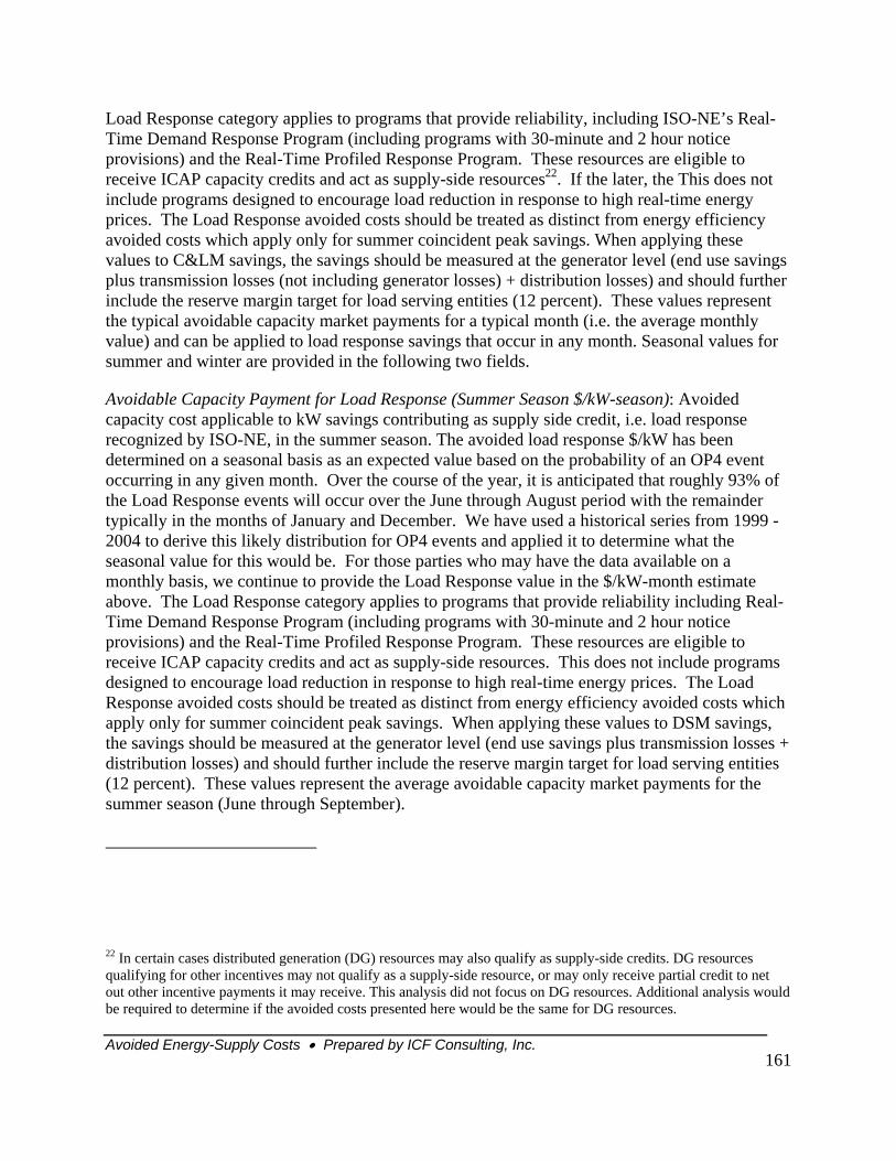
Avoided Energy-Supply Costs • Prepared by ICF Consulting, Inc.
161
Load Response category applies to programs that provide reliability, including ISO-NE’s Real-Time Demand Response Program (including programs with 30-minute and 2 hour notice provisions) and the Real-Time Profiled Response Program. These resources are eligible to receive ICAP capacity credits and act as supply-side resources22. If the later, the This does not include programs designed to encourage load reduction in response to high real-time energy prices. The Load Response avoided costs should be treated as distinct from energy efficiency avoided costs which apply only for summer coincident peak savings. When applying these values to C&LM savings, the savings should be measured at the generator level (end use savings plus transmission losses (not including generator losses) + distribution losses) and should further include the reserve margin target for load serving entities (12 percent). These values represent the typical avoidable capacity market payments for a typical month (i.e. the average monthly value) and can be applied to load response savings that occur in any month. Seasonal values for summer and winter are provided in the following two fields.
Avoidable Capacity Payment for Load Response (Summer Season $/kW-season): Avoided capacity cost applicable to kW savings contributing as supply side credit, i.e. load response recognized by ISO-NE, in the summer season. The avoided load response $/kW has been determined on a seasonal basis as an expected value based on the probability of an OP4 event occurring in any given month. Over the course of the year, it is anticipated that roughly 93% of the Load Response events will occur over the June through August period with the remainder typically in the months of January and December. We have used a historical series from 1999 - 2004 to derive this likely distribution for OP4 events and applied it to determine what the seasonal value for this would be. For those parties who may have the data available on a monthly basis, we continue to provide the Load Response value in the $/kW-month estimate above. The Load Response category applies to programs that provide reliability including Real-Time Demand Response Program (including programs with 30-minute and 2 hour notice provisions) and the Real-Time Profiled Response Program. These resources are eligible to receive ICAP capacity credits and act as supply-side resources. This does not include programs designed to encourage load reduction in response to high real-time energy prices. The Load Response avoided costs should be treated as distinct from energy efficiency avoided costs which apply only for summer coincident peak savings. When applying these values to DSM savings, the savings should be measured at the generator level (end use savings plus transmission losses + distribution losses) and should further include the reserve margin target for load serving entities (12 percent). These values represent the average avoidable capacity market payments for the summer season (June through September).
22 In certain cases distributed generation (DG) resources may also qualify as supply-side credits. DG resources qualifying for other incentives may not qualify as a supply-side resource, or may only receive partial credit to net out other incentive payments it may receive. This analysis did not focus on DG resources. Additional analysis would be required to determine if the avoided costs presented here would be the same for DG resources.

Avoided Energy-Supply Costs • Prepared by ICF Consulting, Inc.
162
Avoidable Capacity Payment for Load Response (Winter Season $/kW-season): Avoided capacity cost applicable to KW savings contributing as supply side credit, i.e. load response recognized by ISO-NE, in the winter season. The avoided load response $/kW has been determined on a seasonal basis as an expected value based on the probability of an OP4 event occurring in any given month. Over the course of the year, it is anticipated that roughly 93% of the Load Response events will occur over the June through August period with the remainder typically in the months of January and December. We have used a historical series from 1999 - 2004 to derive this likely distribution for OP4 events and applied it to determine what the seasonal value for this would be. For those parties who may have the data available on a monthly basis, we continue to provide the Load Response value in the $/kW-month estimate. The Load Response category applies to programs that provide reliability including Real-Time Demand Response Program (including programs with 30-minute and 2 hour notice provisions) and the Real-Time Profiled Response Program. These resources are eligible to receive ICAP capacity credits and act as supply-side resources. This does not include programs designed to encourage load reduction in response to high real-time energy prices. The Load Response avoided costs should be treated as distinct from energy efficiency avoided costs which apply only for summer coincident peak savings. When applying these values to DSM savings, the savings should be measured at the generator level (end use savings plus transmission losses + distribution losses) and should further include the reserve margin target for load serving entities (12 percent). These values represent the average avoidable capacity market payments for the winter season (January through May and October through December).
Avoidable Capacity Payment at Energy Efficiency at Summer Coincident Peak ($/kW-yr): Avoided Cost applicable to kW savings from C&LM programs at summer coincident peak. Based on a review of a long-term series of the timing of summer coincident peak, June, July and August are the months when peak is expected to occur. The peak hour is anticipated to be between 3pm and 5pm on a weekday in these months. Programs targeted to the peak hours will be able to contribute to capacity costs reductions. Savings from programs should be measured at the generator level when determining the total savings. To convert kilowatt reductions at the end use level to the generator level (after generator losses), the reserve margin credit and transmission and distribution losses should be applied to the actual load reduction. The value presented here for use in the screening models is the equivalent of the Annual Capacity Value described above.
Load Response (at any month $/kWh): This field provides the “Capacity Value at Load Response” for load response resources (see above for definition of load response resource) in $/kWh. The annual load response avoidable cost has been converted to $/kWh using a 100 percent load factor. This field is provided for information purposes to illustrate costs at the kWh level.
Energy Efficiency at Summer Coincident Peak ($/kWh): The “Avoidable Capacity Payment at Energy Efficiency at Summer Coincident Peak” is converted to $/kWh using a 100 percent load factor. This represents the average hourly avoided cost for all hours (8760 hours). This field is provided for information purposes to illustrate costs at the kWh level.
DRIPE 0.75% Capacity Price ($/kW-yr): The incremental avoided capacity payment related to
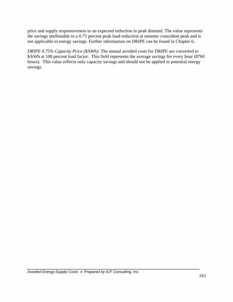
Avoided Energy-Supply Costs • Prepared by ICF Consulting, Inc.
163
price and supply responsiveness to an expected reduction in peak demand. The value represents the savings attributable to a 0.75 percent peak load reduction at summer coincident peak and is not applicable to energy savings. Further information on DRIPE can be found in Chapter 6.
DRIPE 0.75% Capacity Price ($/kWh): The annual avoided costs for DRIPE are converted to $/kWh at 100 percent load factor. This field represents the average savings for every hour (8760 hours). This value reflects only capacity savings and should not be applied to potential energy savings.
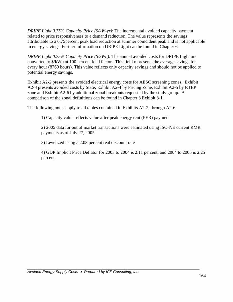
Avoided Energy-Supply Costs • Prepared by ICF Consulting, Inc.
164
DRIPE Light 0.75% Capacity Price ($/kW-yr): The incremental avoided capacity payment related to price responsiveness to a demand reduction. The value represents the savings attributable to a 0.75percent peak load reduction at summer coincident peak and is not applicable to energy savings. Further information on DRIPE Light can be found in Chapter 6.
DRIPE Light 0.75% Capacity Price ($/kWh): The annual avoided costs for DRIPE Light are converted to $/kWh at 100 percent load factor. This field represents the average savings for every hour (8760 hours). This value reflects only capacity savings and should not be applied to potential energy savings.
Exhibit A2-2 presents the avoided electrical energy costs for AESC screening zones. Exhibit A2-3 presents avoided costs by State, Exhibit A2-4 by Pricing Zone, Exhibit A2-5 by RTEP zone and Exhibit A2-6 by additional zonal breakouts requested by the study group. A comparison of the zonal definitions can be found in Chapter 3 Exhibit 3-1.
The following notes apply to all tables contained in Exhibits A2-2, through A2-6:
1) Capacity value reflects value after peak energy rent (PER) payment
2) 2005 data for out of market transactions were estimated using ISO-NE current RMR payments as of July 27, 2005
3) Levelized using a 2.03 percent real discount rate
4) GDP Implicit Price Deflator for 2003 to 2004 is 2.11 percent, and 2004 to 2005 is 2.25 percent.
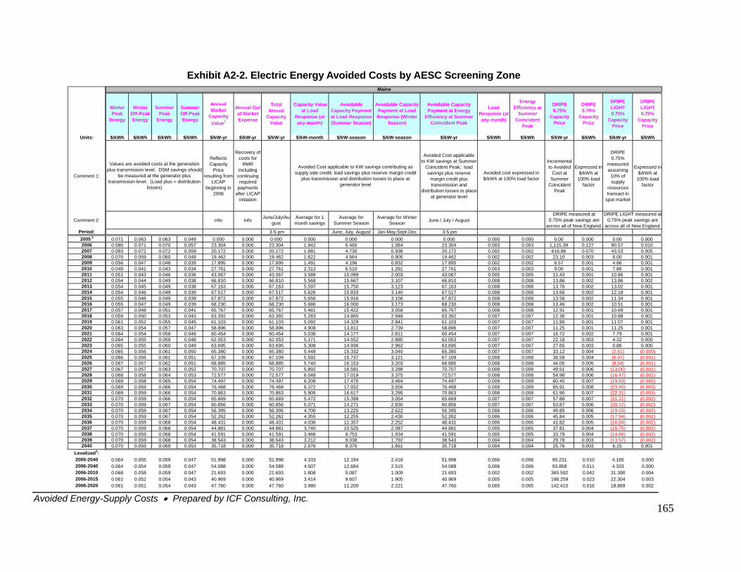
Avoided Energy-Supply Costs • Prepared by ICF Consulting, Inc.
165
Exhibit A2-2. Electric Energy Avoided Costs by AESC Screening Zone
Winter Peak
Energy
Winter Off-Peak Energy
Summer Peak
Energy
Summer Off-Peak Energy
Annual Market
Capacity Value1
Annual Out of Market Expense
Total Annual
Capacity Value
Capacity Value at Load
Response (at any month)
Avoidable Capacity Payment at Load Response (Summer Season)
Avoidable Capacity Payment at Load Response (Winter
Season)
Avoidable Capacity Payment at Energy
Efficiency at Summer Coincident Peak
Load Response (at any month)
Energy Efficiency at
Summer Coincident
Peak
DRIPE 0.75%
Capacity Price
DRIPE 0.75%
Capacity Price
DRIPE LIGHT 0.75%
Capacity Price
DRIPE LIGHT 0.75%
Capacity Price
Units: $/kWh $/kWh $/kWh $/kWh $/kW-yr $/kW-yr $/kW-yr $/kW-month $/kW-season $/kW-season $/kW-yr $/kWh $/kWh $/kW-yr $/kWh $/kW-yr $/kWh
Comment 1:
Reflects Capacity
Price resulting from
LICAP beginning in
2006
Recovery of costs for
RMR including
continuing required
payments after LICAP
initiation
Avoided Cost applicable to KW savings at Summer
Coincident Peak; load savings plus reserve
margin credit plus transmission and
distribution losses to place at generator level
Incremental to Avoided
Cost at Summer
Coincident Peak
Expressed in $/kWh at
100% load factor
DRIPE 0.75%
measured assuming
10% of supply
resources transact in
spot market
Expressed in $/kWh at
100% load factor
Comment 2: info info June/July/August
Average for 1 month savings
Average for Summer Season
Average for Winter Season June / July / August
Period: 3-5 pm June, July, August Jan-May;Sept-Dec 3-5 pm2005 2 0.071 0.063 0.063 0.049 0.000 0.000 0.000 0.000 0.000 0.000 0.000 0.000 0.000 0.00 0.000 0.00 0.0002006 0.080 0.071 0.070 0.057 23.304 0.000 23.304 1.942 5.465 1.084 23.304 0.003 0.003 1,115.39 0.127 90.57 0.0102007 0.083 0.072 0.072 0.059 20.172 0.000 20.172 1.681 4.730 0.938 20.172 0.002 0.002 616.86 0.070 43.53 0.0052008 0.070 0.059 0.060 0.048 19.462 0.000 19.462 1.622 4.564 0.905 19.462 0.002 0.002 23.10 0.003 6.00 0.0012009 0.056 0.047 0.048 0.039 17.895 0.000 17.895 1.491 4.196 0.832 17.895 0.002 0.002 6.57 0.001 4.86 0.0012010 0.049 0.041 0.043 0.034 27.761 0.000 27.761 2.313 6.510 1.291 27.761 0.003 0.003 9.00 0.001 7.86 0.0012011 0.051 0.043 0.046 0.036 43.067 0.000 43.067 3.589 10.099 2.003 43.067 0.005 0.005 11.43 0.001 10.86 0.0012012 0.054 0.044 0.049 0.038 66.810 0.000 66.810 5.568 15.667 3.107 66.810 0.008 0.008 13.86 0.002 13.86 0.0022013 0.054 0.045 0.049 0.038 67.163 0.000 67.163 5.597 15.750 3.123 67.163 0.008 0.008 13.76 0.002 13.02 0.0012014 0.054 0.046 0.049 0.039 67.517 0.000 67.517 5.626 15.833 3.140 67.517 0.008 0.008 13.66 0.002 12.18 0.0012015 0.055 0.046 0.049 0.039 67.872 0.000 67.872 5.656 15.916 3.156 67.872 0.008 0.008 13.56 0.002 11.34 0.0012016 0.055 0.047 0.049 0.039 68.230 0.000 68.230 5.686 16.000 3.173 68.230 0.008 0.008 13.46 0.002 10.51 0.0012017 0.057 0.048 0.051 0.041 65.767 0.000 65.767 5.481 15.422 3.058 65.767 0.008 0.008 12.91 0.001 10.69 0.0012018 0.059 0.050 0.053 0.043 63.392 0.000 63.392 5.283 14.865 2.948 63.392 0.007 0.007 12.36 0.001 10.88 0.0012019 0.061 0.052 0.055 0.045 61.103 0.000 61.103 5.092 14.329 2.841 61.103 0.007 0.007 11.80 0.001 11.07 0.0012020 0.063 0.054 0.057 0.047 58.896 0.000 58.896 4.908 13.811 2.739 58.896 0.007 0.007 11.25 0.001 11.25 0.0012021 0.064 0.054 0.058 0.048 60.454 0.000 60.454 5.038 14.177 2.811 60.454 0.007 0.007 16.72 0.002 7.79 0.0012022 0.064 0.055 0.059 0.048 62.053 0.000 62.053 5.171 14.552 2.885 62.053 0.007 0.007 22.18 0.003 4.32 0.0002023 0.065 0.055 0.060 0.049 63.695 0.000 63.695 5.308 14.936 2.962 63.695 0.007 0.007 27.65 0.003 0.86 0.0002024 0.065 0.056 0.061 0.050 65.380 0.000 65.380 5.448 15.332 3.040 65.380 0.007 0.007 33.12 0.004 (2.61) (0.000)
(6.07) (0.001)(9.54) (0.001)
(13.00) (0.001)(16.47) (0.002)(19.93) (0.002)(23.40) (0.003)(22.31) (0.003)(21.21) (0.002)(20.12) (0.002)(19.03) (0.002)(17.94) (0.002)(16.84) (0.002)(15.75) (0.002)(14.66) (0.002)(13.57) (0.002)6.15 0.001
2025 0.066 0.056 0.061 0.051 67.109 0.000 67.109 5.592 15.737 3.121 67.109 0.008 0.008 38.58 0.0042026 0.067 0.057 0.062 0.051 68.885 0.000 68.885 5.740 16.153 3.203 68.885 0.008 0.008 44.05 0.0052027 0.067 0.057 0.063 0.052 70.707 0.000 70.707 5.892 16.581 3.288 70.707 0.008 0.008 49.51 0.0062028 0.068 0.058 0.064 0.053 72.577 0.000 72.577 6.048 17.019 3.375 72.577 0.008 0.008 54.98 0.0062029 0.069 0.058 0.065 0.054 74.497 0.000 74.497 6.208 17.470 3.464 74.497 0.009 0.009 60.45 0.0072030 0.069 0.059 0.066 0.054 76.468 0.000 76.468 6.372 17.932 3.556 76.468 0.009 0.009 65.91 0.0082031 0.069 0.059 0.066 0.054 70.863 0.000 70.863 5.905 16.617 3.295 70.863 0.008 0.008 61.90 0.0072032 0.070 0.059 0.066 0.054 65.669 0.000 65.669 5.472 15.399 3.054 65.669 0.007 0.007 57.88 0.0072033 0.070 0.059 0.067 0.054 60.856 0.000 60.856 5.071 14.271 2.830 60.856 0.007 0.007 53.87 0.0062034 0.070 0.059 0.067 0.054 56.395 0.000 56.395 4.700 13.225 2.622 56.395 0.006 0.006 49.85 0.0062035 0.070 0.059 0.067 0.054 52.262 0.000 52.262 4.355 12.255 2.430 52.262 0.006 0.006 45.84 0.0052036 0.070 0.059 0.068 0.054 48.431 0.000 48.431 4.036 11.357 2.252 48.431 0.006 0.006 41.82 0.0052037 0.070 0.059 0.068 0.054 44.881 0.000 44.881 3.740 10.525 2.087 44.881 0.005 0.005 37.81 0.0042038 0.070 0.059 0.068 0.054 41.591 0.000 41.591 3.466 9.753 1.934 41.591 0.005 0.005 33.79 0.0042039 0.070 0.059 0.068 0.054 38.543 0.000 38.543 3.212 9.038 1.792 38.543 0.004 0.004 29.78 0.0032040 0.070 0.059 0.069 0.053 35.718 0.000 35.718 2.976 8.376 1.661 35.718 0.004 0.004 25.76 0.003
Levelized3: 2005-2040 0.064 0.055 0.059 0.047 51.998 0.000 51.998 4.333 12.194 2.418 51.998 0.006 0.006 90.231 0.010 4.165 0.0002006-2040 0.064 0.054 0.059 0.047 54.088 0.000 54.088 4.507 12.684 2.515 54.088 0.006 0.006 93.858 0.011 4.333 0.0002006-2010 0.068 0.058 0.059 0.047 21.693 0.000 21.693 1.808 5.087 1.009 21.693 0.002 0.002 365.592 0.042 31.390 0.0042006-2015 0.061 0.052 0.054 0.043 40.969 0.000 40.969 3.414 9.607 1.905 40.969 0.005 0.005 198.259 0.023 22.304 0.0032006-2020 0.061 0.051 0.054 0.043 47.760 0.000 47.760 3.980 11.200 2.221 47.760 0.005 0.005 142.410 0.016 18.869 0.002
Avoided Cost applicable to KW savings contributing as supply side credit; load savings plus reserve margin credit
plus transmission and distribution losses to place at generator level
Values are avoided costs at the generation plus transmission level. DSM savings should
be measured at the generator plus transmission level. (Load plus + distribution
losses)
Avoided cost expressed in $/kWh at 100% load factor
Maine
DRIPE measured at 0.75% peak savings are
across all of New England.
DRIPE LIGHT measured at 0.75% peak savings are
across all of New England.
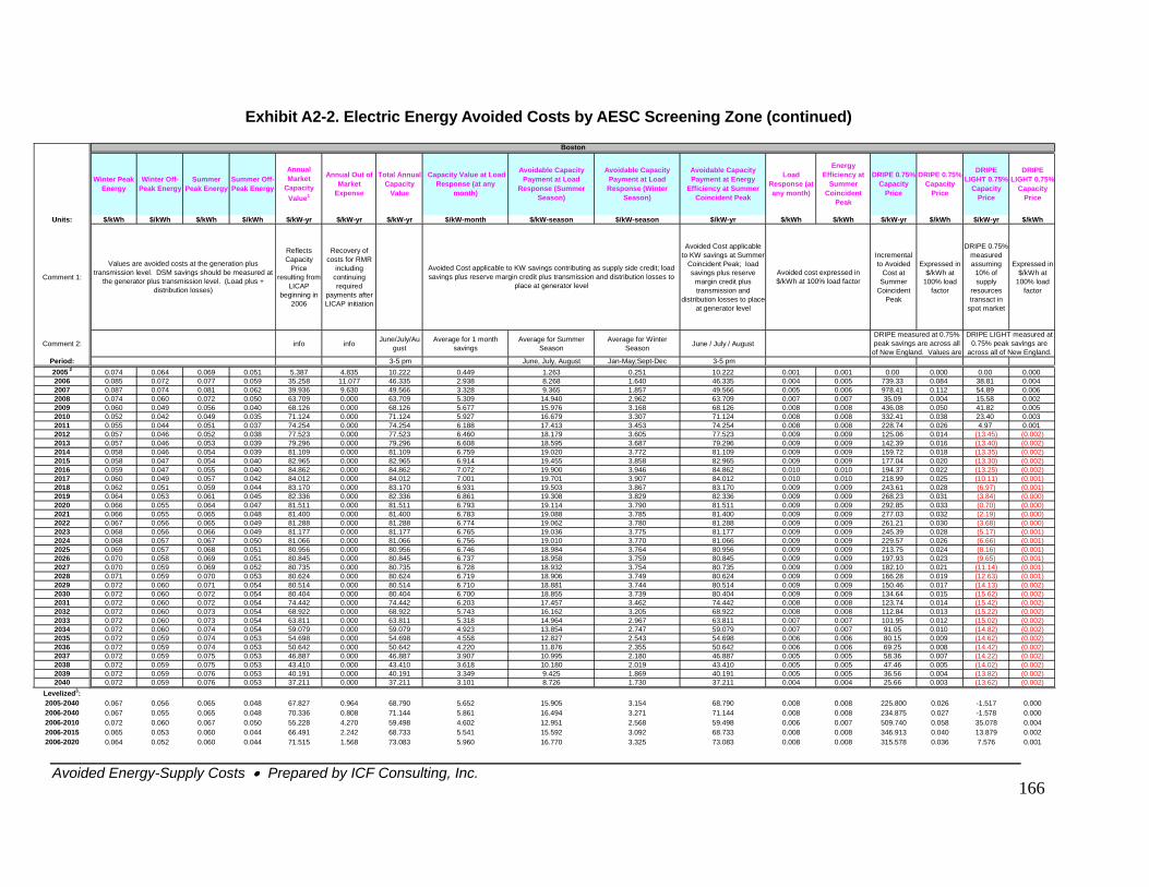
Avoided Energy-Supply Costs • Prepared by ICF Consulting, Inc.
166
Exhibit A2-2. Electric Energy Avoided Costs by AESC Screening Zone (continued)
Winter Peak Energy
Winter Off-Peak Energy
Summer Peak Energy
Summer Off-Peak Energy
Annual Market
Capacity Value1
Annual Out of Market
Expense
Total Annual Capacity
Value
Capacity Value at Load Response (at any
month)
Avoidable Capacity Payment at Load
Response (Summer Season)
Avoidable Capacity Payment at Load Response (Winter
Season)
Avoidable Capacity Payment at Energy
Efficiency at Summer Coincident Peak
Load Response (at any month)
Energy Efficiency at
Summer Coincident
Peak
DRIPE 0.75% Capacity
Price
DRIPE 0.75% Capacity
Price
DRIPE LIGHT 0.75%
Capacity Price
DRIPE LIGHT 0.75%
Capacity Price
Units: $/kWh $/kWh $/kWh $/kWh $/kW-yr $/kW-yr $/kW-yr $/kW-month $/kW-season $/kW-season $/kW-yr $/kWh $/kWh $/kW-yr $/kWh $/kW-yr $/kWh
Comment 1:
Reflects Capacity
Price resulting from
LICAP beginning in
2006
Recovery of costs for RMR
including continuing required
payments after LICAP initiation
Avoided Cost applicable to KW savings at Summer
Coincident Peak; load savings plus reserve
margin credit plus transmission and
distribution losses to place at generator level
Incremental to Avoided
Cost at Summer
Coincident Peak
Expressed in $/kWh at
100% load factor
DRIPE 0.75% measured assuming
10% of supply
resources transact in
spot market
Expressed in $/kWh at
100% load factor
Comment 2: info info June/July/August
Average for 1 month savings
Average for Summer Season
Average for Winter Season June / July / August
Period: 3-5 pm June, July, August Jan-May;Sept-Dec 3-5 pm2005 2 0.074 0.064 0.069 0.051 5.387 4.835 10.222 0.449 1.263 0.251 10.222 0.001 0.001 0.00 0.000 0.00 0.0002006 0.085 0.072 0.077 0.059 35.258 11.077 46.335 2.938 8.268 1.640 46.335 0.004 0.005 739.33 0.084 38.81 0.0042007 0.087 0.074 0.081 0.062 39.936 9.630 49.566 3.328 9.365 1.857 49.566 0.005 0.006 978.41 0.112 54.89 0.0062008 0.074 0.060 0.072 0.050 63.709 0.000 63.709 5.309 14.940 2.962 63.709 0.007 0.007 35.09 0.004 15.58 0.0022009 0.060 0.049 0.056 0.040 68.126 0.000 68.126 5.677 15.976 3.168 68.126 0.008 0.008 436.08 0.050 41.82 0.0052010 0.052 0.042 0.049 0.035 71.124 0.000 71.124 5.927 16.679 3.307 71.124 0.008 0.008 332.41 0.038 23.40 0.0032011 0.055 0.044 0.051 0.037 74.254 0.000 74.254 6.188 17.413 3.453 74.254 0.008 0.008 228.74 0.026 4.97 0.0012012 0.057 0.046 0.052 0.038 77.523 0.000 77.523 6.460 18.179 3.605 77.523 0.009 0.009 125.06 0.014 (13.45) (0.002)
(13.40) (0.002)(13.35) (0.002)(13.30) (0.002)(13.25) (0.002)(10.11) (0.001)(6.97) (0.001)(3.84) (0.000)(0.70) (0.000)(2.19) (0.000)(3.68) (0.000)(5.17) (0.001)(6.66) (0.001)(8.16) (0.001)(9.65) (0.001)(11.14) (0.001)(12.63) (0.001)(14.13) (0.002)(15.62) (0.002)(15.42) (0.002)(15.22) (0.002)(15.02) (0.002)(14.82) (0.002)(14.62) (0.002)(14.42) (0.002)(14.22) (0.002)(14.02) (0.002)(13.82) (0.002)(13.62) (0.002)
2013 0.057 0.046 0.053 0.039 79.296 0.000 79.296 6.608 18.595 3.687 79.296 0.009 0.009 142.39 0.0162014 0.058 0.046 0.054 0.039 81.109 0.000 81.109 6.759 19.020 3.772 81.109 0.009 0.009 159.72 0.0182015 0.058 0.047 0.054 0.040 82.965 0.000 82.965 6.914 19.455 3.858 82.965 0.009 0.009 177.04 0.0202016 0.059 0.047 0.055 0.040 84.862 0.000 84.862 7.072 19.900 3.946 84.862 0.010 0.010 194.37 0.0222017 0.060 0.049 0.057 0.042 84.012 0.000 84.012 7.001 19.701 3.907 84.012 0.010 0.010 218.99 0.0252018 0.062 0.051 0.059 0.044 83.170 0.000 83.170 6.931 19.503 3.867 83.170 0.009 0.009 243.61 0.0282019 0.064 0.053 0.061 0.045 82.336 0.000 82.336 6.861 19.308 3.829 82.336 0.009 0.009 268.23 0.0312020 0.066 0.055 0.064 0.047 81.511 0.000 81.511 6.793 19.114 3.790 81.511 0.009 0.009 292.85 0.0332021 0.066 0.055 0.065 0.048 81.400 0.000 81.400 6.783 19.088 3.785 81.400 0.009 0.009 277.03 0.0322022 0.067 0.056 0.065 0.049 81.288 0.000 81.288 6.774 19.062 3.780 81.288 0.009 0.009 261.21 0.0302023 0.068 0.056 0.066 0.049 81.177 0.000 81.177 6.765 19.036 3.775 81.177 0.009 0.009 245.39 0.0282024 0.068 0.057 0.067 0.050 81.066 0.000 81.066 6.756 19.010 3.770 81.066 0.009 0.009 229.57 0.0262025 0.069 0.057 0.068 0.051 80.956 0.000 80.956 6.746 18.984 3.764 80.956 0.009 0.009 213.75 0.0242026 0.070 0.058 0.069 0.051 80.845 0.000 80.845 6.737 18.958 3.759 80.845 0.009 0.009 197.93 0.0232027 0.070 0.059 0.069 0.052 80.735 0.000 80.735 6.728 18.932 3.754 80.735 0.009 0.009 182.10 0.0212028 0.071 0.059 0.070 0.053 80.624 0.000 80.624 6.719 18.906 3.749 80.624 0.009 0.009 166.28 0.0192029 0.072 0.060 0.071 0.054 80.514 0.000 80.514 6.710 18.881 3.744 80.514 0.009 0.009 150.46 0.0172030 0.072 0.060 0.072 0.054 80.404 0.000 80.404 6.700 18.855 3.739 80.404 0.009 0.009 134.64 0.0152031 0.072 0.060 0.072 0.054 74.442 0.000 74.442 6.203 17.457 3.462 74.442 0.008 0.008 123.74 0.0142032 0.072 0.060 0.073 0.054 68.922 0.000 68.922 5.743 16.162 3.205 68.922 0.008 0.008 112.84 0.0132033 0.072 0.060 0.073 0.054 63.811 0.000 63.811 5.318 14.964 2.967 63.811 0.007 0.007 101.95 0.0122034 0.072 0.060 0.074 0.054 59.079 0.000 59.079 4.923 13.854 2.747 59.079 0.007 0.007 91.05 0.0102035 0.072 0.059 0.074 0.053 54.698 0.000 54.698 4.558 12.827 2.543 54.698 0.006 0.006 80.15 0.0092036 0.072 0.059 0.074 0.053 50.642 0.000 50.642 4.220 11.876 2.355 50.642 0.006 0.006 69.25 0.0082037 0.072 0.059 0.075 0.053 46.887 0.000 46.887 3.907 10.995 2.180 46.887 0.005 0.005 58.36 0.0072038 0.072 0.059 0.075 0.053 43.410 0.000 43.410 3.618 10.180 2.019 43.410 0.005 0.005 47.46 0.0052039 0.072 0.059 0.076 0.053 40.191 0.000 40.191 3.349 9.425 1.869 40.191 0.005 0.005 36.56 0.0042040 0.072 0.059 0.076 0.053 37.211 0.000 37.211 3.101 8.726 1.730 37.211 0.004 0.004 25.66 0.003
Levelized3: 2005-2040 0.067 0.056 0.065 0.048 67.827 0.964 68.790 5.652 15.905 3.154 68.790 0.008 0.008 225.800 0.026 -1.517 0.0002006-2040 0.067 0.055 0.065 0.048 70.336 0.808 71.144 5.861 16.494 3.271 71.144 0.008 0.008 234.875 0.027 -1.578 0.0002006-2010 0.072 0.060 0.067 0.050 55.228 4.270 59.498 4.602 12.951 2.568 59.498 0.006 0.007 509.740 0.058 35.078 0.0042006-2015 0.065 0.053 0.060 0.044 66.491 2.242 68.733 5.541 15.592 3.092 68.733 0.008 0.008 346.913 0.040 13.879 0.0022006-2020 0.064 0.052 0.060 0.044 71.515 1.568 73.083 5.960 16.770 3.325 73.083 0.008 0.008 315.578 0.036 7.576 0.001
Boston
DRIPE measured at 0.75% peak savings are across all
of New England. Values are
Avoided Cost applicable to KW savings contributing as supply side credit; load savings plus reserve margin credit plus transmission and distribution losses to
place at generator level
DRIPE LIGHT measured at 0.75% peak savings are
across all of New England.
Values are avoided costs at the generation plus transmission level. DSM savings should be measured at
the generator plus transmission level. (Load plus + distribution losses)
Avoided cost expressed in $/kWh at 100% load factor
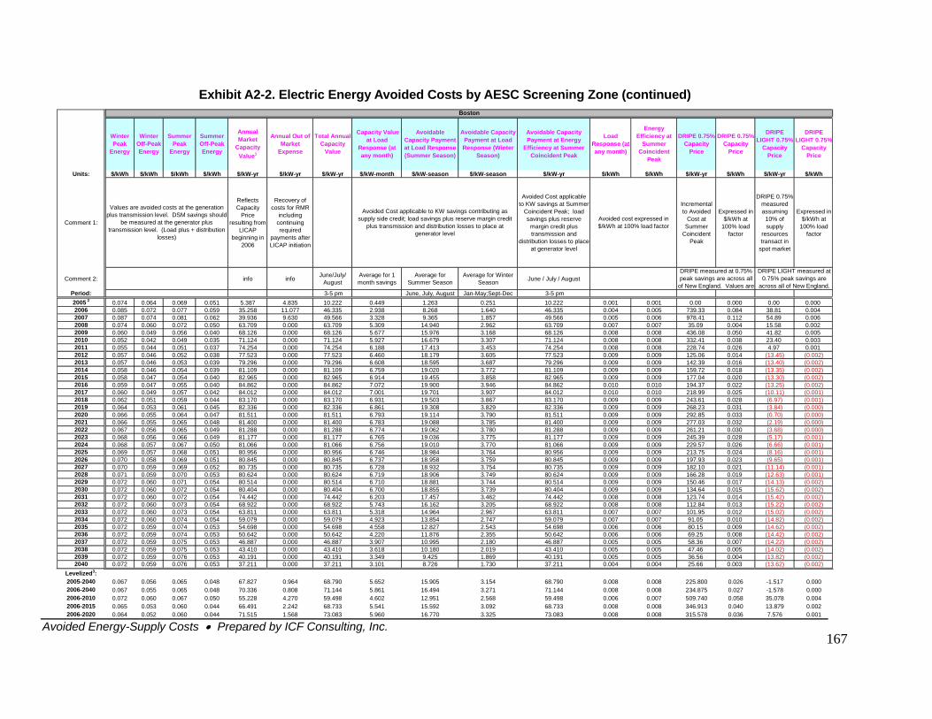
Avoided Energy-Supply Costs • Prepared by ICF Consulting, Inc.
167
Exhibit A2-2. Electric Energy Avoided Costs by AESC Screening Zone (continued)
Winter Peak
Energy
Winter Off-Peak Energy
Summer Peak
Energy
Summer Off-Peak Energy
Annual Market
Capacity Value1
Annual Out of Market
Expense
Total Annual Capacity
Value
Capacity Value at Load
Response (at any month)
Avoidable Capacity Payment at Load Response (Summer Season)
Avoidable Capacity Payment at Load Response (Winter
Season)
Avoidable Capacity Payment at Energy
Efficiency at Summer Coincident Peak
Load Response (at any month)
Energy Efficiency at
Summer Coincident
Peak
DRIPE 0.75% Capacity
Price
DRIPE 0.75% Capacity
Price
DRIPE LIGHT 0.75%
Capacity Price
DRIPE LIGHT 0.75%
Capacity Price
Units: $/kWh $/kWh $/kWh $/kWh $/kW-yr $/kW-yr $/kW-yr $/kW-month $/kW-season $/kW-season $/kW-yr $/kWh $/kWh $/kW-yr $/kWh $/kW-yr $/kWh
Comment 1:
Reflects Capacity
Price resulting from
LICAP beginning in
2006
Recovery of costs for RMR
including continuing required
payments after LICAP initiation
Avoided Cost applicable to KW savings at Summer
Coincident Peak; load savings plus reserve
margin credit plus transmission and
distribution losses to place at generator level
Incremental to Avoided
Cost at Summer
Coincident Peak
Expressed in $/kWh at
100% load factor
DRIPE 0.75% measured assuming
10% of supply
resources transact in
spot market
Expressed in $/kWh at
100% load factor
Comment 2: info info June/July/ August
Average for 1 month savings
Average for Summer Season
Average for Winter Season June / July / August
Period: 3-5 pm June, July, August Jan-May;Sept-Dec 3-5 pm2005 2 0.074 0.064 0.069 0.051 5.387 4.835 10.222 0.449 1.263 0.251 10.222 0.001 0.001 0.00 0.000 0.00 0.0002006 0.085 0.072 0.077 0.059 35.258 11.077 46.335 2.938 8.268 1.640 46.335 0.004 0.005 739.33 0.084 38.81 0.0042007 0.087 0.074 0.081 0.062 39.936 9.630 49.566 3.328 9.365 1.857 49.566 0.005 0.006 978.41 0.112 54.89 0.0062008 0.074 0.060 0.072 0.050 63.709 0.000 63.709 5.309 14.940 2.962 63.709 0.007 0.007 35.09 0.004 15.58 0.0022009 0.060 0.049 0.056 0.040 68.126 0.000 68.126 5.677 15.976 3.168 68.126 0.008 0.008 436.08 0.050 41.82 0.0052010 0.052 0.042 0.049 0.035 71.124 0.000 71.124 5.927 16.679 3.307 71.124 0.008 0.008 332.41 0.038 23.40 0.0032011 0.055 0.044 0.051 0.037 74.254 0.000 74.254 6.188 17.413 3.453 74.254 0.008 0.008 228.74 0.026 4.97 0.0012012 0.057 0.046 0.052 0.038 77.523 0.000 77.523 6.460 18.179 3.605 77.523 0.009 0.009 125.06 0.014 (13.45) (0.002)
(13.40) (0.002)(13.35) (0.002)(13.30) (0.002)(13.25) (0.002)(10.11) (0.001)(6.97) (0.001)(3.84) (0.000)(0.70) (0.000)(2.19) (0.000)(3.68) (0.000)(5.17) (0.001)(6.66) (0.001)(8.16) (0.001)(9.65) (0.001)
(11.14) (0.001)(12.63) (0.001)(14.13) (0.002)(15.62) (0.002)(15.42) (0.002)(15.22) (0.002)(15.02) (0.002)(14.82) (0.002)(14.62) (0.002)(14.42) (0.002)(14.22) (0.002)(14.02) (0.002)(13.82) (0.002)(13.62) (0.002)
2013 0.057 0.046 0.053 0.039 79.296 0.000 79.296 6.608 18.595 3.687 79.296 0.009 0.009 142.39 0.0162014 0.058 0.046 0.054 0.039 81.109 0.000 81.109 6.759 19.020 3.772 81.109 0.009 0.009 159.72 0.0182015 0.058 0.047 0.054 0.040 82.965 0.000 82.965 6.914 19.455 3.858 82.965 0.009 0.009 177.04 0.0202016 0.059 0.047 0.055 0.040 84.862 0.000 84.862 7.072 19.900 3.946 84.862 0.010 0.010 194.37 0.0222017 0.060 0.049 0.057 0.042 84.012 0.000 84.012 7.001 19.701 3.907 84.012 0.010 0.010 218.99 0.0252018 0.062 0.051 0.059 0.044 83.170 0.000 83.170 6.931 19.503 3.867 83.170 0.009 0.009 243.61 0.0282019 0.064 0.053 0.061 0.045 82.336 0.000 82.336 6.861 19.308 3.829 82.336 0.009 0.009 268.23 0.0312020 0.066 0.055 0.064 0.047 81.511 0.000 81.511 6.793 19.114 3.790 81.511 0.009 0.009 292.85 0.0332021 0.066 0.055 0.065 0.048 81.400 0.000 81.400 6.783 19.088 3.785 81.400 0.009 0.009 277.03 0.0322022 0.067 0.056 0.065 0.049 81.288 0.000 81.288 6.774 19.062 3.780 81.288 0.009 0.009 261.21 0.0302023 0.068 0.056 0.066 0.049 81.177 0.000 81.177 6.765 19.036 3.775 81.177 0.009 0.009 245.39 0.0282024 0.068 0.057 0.067 0.050 81.066 0.000 81.066 6.756 19.010 3.770 81.066 0.009 0.009 229.57 0.0262025 0.069 0.057 0.068 0.051 80.956 0.000 80.956 6.746 18.984 3.764 80.956 0.009 0.009 213.75 0.0242026 0.070 0.058 0.069 0.051 80.845 0.000 80.845 6.737 18.958 3.759 80.845 0.009 0.009 197.93 0.0232027 0.070 0.059 0.069 0.052 80.735 0.000 80.735 6.728 18.932 3.754 80.735 0.009 0.009 182.10 0.0212028 0.071 0.059 0.070 0.053 80.624 0.000 80.624 6.719 18.906 3.749 80.624 0.009 0.009 166.28 0.0192029 0.072 0.060 0.071 0.054 80.514 0.000 80.514 6.710 18.881 3.744 80.514 0.009 0.009 150.46 0.0172030 0.072 0.060 0.072 0.054 80.404 0.000 80.404 6.700 18.855 3.739 80.404 0.009 0.009 134.64 0.0152031 0.072 0.060 0.072 0.054 74.442 0.000 74.442 6.203 17.457 3.462 74.442 0.008 0.008 123.74 0.0142032 0.072 0.060 0.073 0.054 68.922 0.000 68.922 5.743 16.162 3.205 68.922 0.008 0.008 112.84 0.0132033 0.072 0.060 0.073 0.054 63.811 0.000 63.811 5.318 14.964 2.967 63.811 0.007 0.007 101.95 0.0122034 0.072 0.060 0.074 0.054 59.079 0.000 59.079 4.923 13.854 2.747 59.079 0.007 0.007 91.05 0.0102035 0.072 0.059 0.074 0.053 54.698 0.000 54.698 4.558 12.827 2.543 54.698 0.006 0.006 80.15 0.0092036 0.072 0.059 0.074 0.053 50.642 0.000 50.642 4.220 11.876 2.355 50.642 0.006 0.006 69.25 0.0082037 0.072 0.059 0.075 0.053 46.887 0.000 46.887 3.907 10.995 2.180 46.887 0.005 0.005 58.36 0.0072038 0.072 0.059 0.075 0.053 43.410 0.000 43.410 3.618 10.180 2.019 43.410 0.005 0.005 47.46 0.0052039 0.072 0.059 0.076 0.053 40.191 0.000 40.191 3.349 9.425 1.869 40.191 0.005 0.005 36.56 0.0042040 0.072 0.059 0.076 0.053 37.211 0.000 37.211 3.101 8.726 1.730 37.211 0.004 0.004 25.66 0.003
Levelized3: 2005-2040 0.067 0.056 0.065 0.048 67.827 0.964 68.790 5.652 15.905 3.154 68.790 0.008 0.008 225.800 0.026 -1.517 0.0002006-2040 0.067 0.055 0.065 0.048 70.336 0.808 71.144 5.861 16.494 3.271 71.144 0.008 0.008 234.875 0.027 -1.578 0.0002006-2010 0.072 0.060 0.067 0.050 55.228 4.270 59.498 4.602 12.951 2.568 59.498 0.006 0.007 509.740 0.058 35.078 0.0042006-2015 0.065 0.053 0.060 0.044 66.491 2.242 68.733 5.541 15.592 3.092 68.733 0.008 0.008 346.913 0.040 13.879 0.0022006-2020 0.064 0.052 0.060 0.044 71.515 1.568 73.083 5.960 16.770 3.325 73.083 0.008 0.008 315.578 0.036 7.576 0.001
Boston
DRIPE measured at 0.75% peak savings are across all
of New England. Values are
Avoided Cost applicable to KW savings contributing as supply side credit; load savings plus reserve margin credit
plus transmission and distribution losses to place at generator level
DRIPE LIGHT measured at 0.75% peak savings are
across all of New England.
Values are avoided costs at the generation plus transmission level. DSM savings should
be measured at the generator plus transmission level. (Load plus + distribution
losses)
Avoided cost expressed in $/kWh at 100% load factor
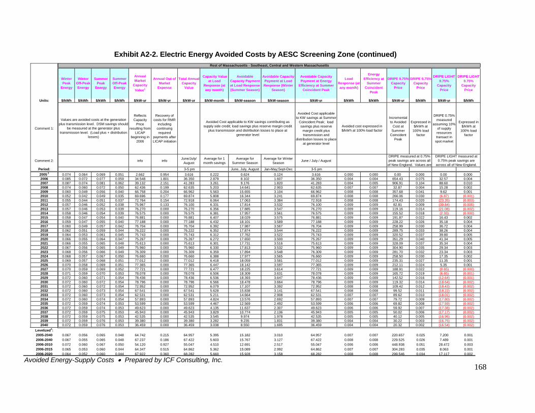
Avoided Energy-Supply Costs • Prepared by ICF Consulting, Inc.
168
Exhibit A2-2. Electric Energy Avoided Costs by AESC Screening Zone (continued)
Winter Peak
Energy
Winter Off-Peak Energy
Summer Peak
Energy
Summer Off-Peak Energy
Annual Market
Capacity Value1
Annual Out of Market
Expense
Total Annual Capacity
Value
Capacity Value at Load
Response (at any month)
Avoidable Capacity Payment at Load Response (Summer Season)
Avoidable Capacity Payment at Load Response (Winter
Season)
Avoidable Capacity Payment at Energy
Efficiency at Summer Coincident Peak
Load Response (at any month)
Energy Efficiency at
Summer Coincident
Peak
DRIPE 0.75% Capacity
Price
DRIPE 0.75% Capacity
Price
DRIPE LIGHT 0.75%
Capacity Price
DRIPE LIGHT 0.75%
Capacity Price
Units: $/kWh $/kWh $/kWh $/kWh $/kW-yr $/kW-yr $/kW-yr $/kW-month $/kW-season $/kW-season $/kW-yr $/kWh $/kWh $/kW-yr $/kWh $/kW-yr $/kWh
Comment 1:
Reflects Capacity
Price resulting from
LICAP beginning in
2006
Recovery of costs for RMR
including continuing required
payments after LICAP initiation
Avoided Cost applicable to KW savings at Summer
Coincident Peak; load savings plus reserve
margin credit plus transmission and
distribution losses to place at generator level
Incremental to Avoided
Cost at Summer
Coincident Peak
Expressed in $/kWh at
100% load factor
DRIPE 0.75% measured
assuming 10% of supply resources transact in
spot market
Expressed in $/kWh at
100% load factor
Comment 2: info info June/July/ August
Average for 1 month savings
Average for Summer Season
Average for Winter Season June / July / August
Period: 3-5 pm June, July, August Jan-May;Sept-Dec 3-5 pm2005 2 0.074 0.064 0.069 0.051 2.662 0.954 3.616 0.222 0.624 0.124 3.616 0.000 0.000 0.00 0.000 0.00 0.0002006 0.085 0.072 0.077 0.059 34.548 1.801 36.350 2.879 8.102 1.607 36.350 0.004 0.004 654.43 0.075 32.57 0.0042007 0.087 0.074 0.081 0.062 39.132 2.151 41.283 3.261 9.176 1.820 41.283 0.004 0.005 906.91 0.104 88.60 0.0102008 0.074 0.060 0.072 0.050 62.436 0.199 62.635 5.203 14.641 2.903 62.635 0.007 0.007 32.87 0.004 15.28 0.0022009 0.060 0.049 0.056 0.040 66.758 0.204 66.962 5.563 15.655 3.104 66.962 0.008 0.008 357.68 0.041 9.62 0.0012010 0.052 0.042 0.049 0.035 69.696 0.177 69.874 5.808 16.344 3.241 69.874 0.008 0.008 266.06 0.030 (6.87) (0.001)
(23.35) (0.003)(39.84) (0.005)(21.08) (0.002)(2.33) (0.000)16.43 0.002
(0.65) (0.000)(6.65) (0.001)
(12.64) (0.001)(18.64) (0.002)(18.43) (0.002)(18.22) (0.002)(18.01) (0.002)(17.80) (0.002)(17.59) (0.002)(17.38) (0.002)(17.17) (0.002)(16.96) (0.002)(16.75) (0.002)(16.54) (0.002)
2011 0.055 0.044 0.051 0.037 72.764 0.154 72.918 6.064 17.063 3.384 72.918 0.008 0.008 174.43 0.0202012 0.057 0.046 0.052 0.038 75.967 0.133 76.100 6.331 17.814 3.532 76.100 0.009 0.009 82.81 0.0092013 0.057 0.046 0.053 0.039 76.270 0.000 76.270 6.356 17.885 3.547 76.270 0.009 0.009 119.16 0.0142014 0.058 0.046 0.054 0.039 76.575 0.000 76.575 6.381 17.957 3.561 76.575 0.009 0.009 155.52 0.0182015 0.058 0.047 0.054 0.040 76.881 0.000 76.881 6.407 18.029 3.575 76.881 0.009 0.009 191.87 0.0222016 0.059 0.047 0.055 0.040 77.188 0.000 77.188 6.432 18.101 3.589 77.188 0.009 0.009 228.22 0.026 35.18 0.0042017 0.060 0.049 0.057 0.042 76.704 0.000 76.704 6.392 17.987 3.567 76.704 0.009 0.009 258.99 0.030 36.72 0.0042018 0.062 0.051 0.059 0.044 76.222 0.000 76.222 6.352 17.874 3.544 76.222 0.009 0.009 289.75 0.033 38.26 0.0042019 0.064 0.053 0.061 0.045 75.743 0.000 75.743 6.312 17.762 3.522 75.743 0.009 0.009 320.52 0.037 39.80 0.0052020 0.066 0.055 0.064 0.047 75.267 0.000 75.267 6.272 17.650 3.500 75.267 0.009 0.009 351.29 0.040 41.34 0.0052021 0.066 0.055 0.065 0.048 75.613 0.000 75.613 6.301 17.731 3.516 75.613 0.009 0.009 328.09 0.037 35.34 0.0042022 0.067 0.056 0.065 0.049 75.960 0.000 75.960 6.330 17.813 3.532 75.960 0.009 0.009 304.90 0.035 29.34 0.0032023 0.068 0.056 0.066 0.049 76.309 0.000 76.309 6.359 17.894 3.548 76.309 0.009 0.009 281.70 0.032 23.34 0.0032024 0.068 0.057 0.067 0.050 76.660 0.000 76.660 6.388 17.977 3.565 76.660 0.009 0.009 258.50 0.030 17.35 0.0022025 0.069 0.057 0.068 0.051 77.012 0.000 77.012 6.418 18.059 3.581 77.012 0.009 0.009 235.31 0.027 11.35 0.0012026 0.070 0.058 0.069 0.051 77.365 0.000 77.365 6.447 18.142 3.597 77.365 0.009 0.009 212.11 0.024 5.35 0.0012027 0.070 0.059 0.069 0.052 77.721 0.000 77.721 6.477 18.225 3.614 77.721 0.009 0.009 188.91 0.0222028 0.071 0.059 0.070 0.053 78.078 0.000 78.078 6.506 18.309 3.631 78.078 0.009 0.009 165.72 0.0192029 0.072 0.060 0.071 0.054 78.436 0.000 78.436 6.536 18.393 3.647 78.436 0.009 0.009 142.52 0.0162030 0.072 0.060 0.072 0.054 78.796 0.000 78.796 6.566 18.478 3.664 78.796 0.009 0.009 119.32 0.0142031 0.072 0.060 0.072 0.054 72.952 0.000 72.952 6.079 17.107 3.392 72.952 0.008 0.008 109.42 0.0122032 0.072 0.060 0.073 0.054 67.541 0.000 67.541 5.628 15.838 3.141 67.541 0.008 0.008 99.52 0.0112033 0.072 0.060 0.073 0.054 62.531 0.000 62.531 5.211 14.664 2.908 62.531 0.007 0.007 89.62 0.0102034 0.072 0.060 0.074 0.054 57.893 0.000 57.893 4.824 13.576 2.692 57.893 0.007 0.007 79.72 0.0092035 0.072 0.059 0.074 0.053 53.599 0.000 53.599 4.467 12.569 2.492 53.599 0.006 0.006 69.82 0.0082036 0.072 0.059 0.074 0.053 49.623 0.000 49.623 4.135 11.637 2.307 49.623 0.006 0.006 59.92 0.0072037 0.072 0.059 0.075 0.053 45.943 0.000 45.943 3.829 10.774 2.136 45.943 0.005 0.005 50.02 0.0062038 0.072 0.059 0.075 0.053 42.535 0.000 42.535 3.545 9.974 1.978 42.535 0.005 0.005 40.12 0.0052039 0.072 0.059 0.076 0.053 39.380 0.000 39.380 3.282 9.235 1.831 39.380 0.004 0.004 30.22 0.0032040 0.072 0.059 0.076 0.053 36.459 0.000 36.459 3.038 8.550 1.695 36.459 0.004 0.004 20.32 0.002
Levelized3: 2005-2040 0.067 0.056 0.065 0.048 64.742 0.215 64.957 5.395 15.182 3.010 64.957 0.007 0.007 220.657 0.025 7.200 0.0012006-2040 0.067 0.055 0.065 0.048 67.237 0.186 67.422 5.603 15.767 3.127 67.422 0.008 0.008 229.525 0.026 7.489 0.0012006-2010 0.072 0.060 0.067 0.050 54.120 0.927 55.047 4.510 12.691 2.517 55.047 0.006 0.006 448.938 0.051 28.472 0.0032006-2015 0.065 0.053 0.060 0.044 64.347 0.515 64.862 5.362 15.089 2.992 64.862 0.007 0.007 304.283 0.035 8.063 0.0012006-2020 0.064 0.052 0.060 0.044 67.922 0.360 68.282 5.660 15.928 3.158 68.282 0.008 0.008 299.546 0.034 17.117 0.002
Rest of Massachusetts - Southeast, Central and Western Massachusetts
Avoided Cost applicable to KW savings contributing as supply side credit; load savings plus reserve margin credit
plus transmission and distribution losses to place at generator level
DRIPE LIGHT measured at 0.75% peak savings are
across all of New England.
Values are avoided costs at the generation plus transmission level. DSM savings should
be measured at the generator plus transmission level. (Load plus + distribution
losses)
Avoided cost expressed in $/kWh at 100% load factor
DRIPE measured at 0.75% peak savings are across all
of New England. Values are
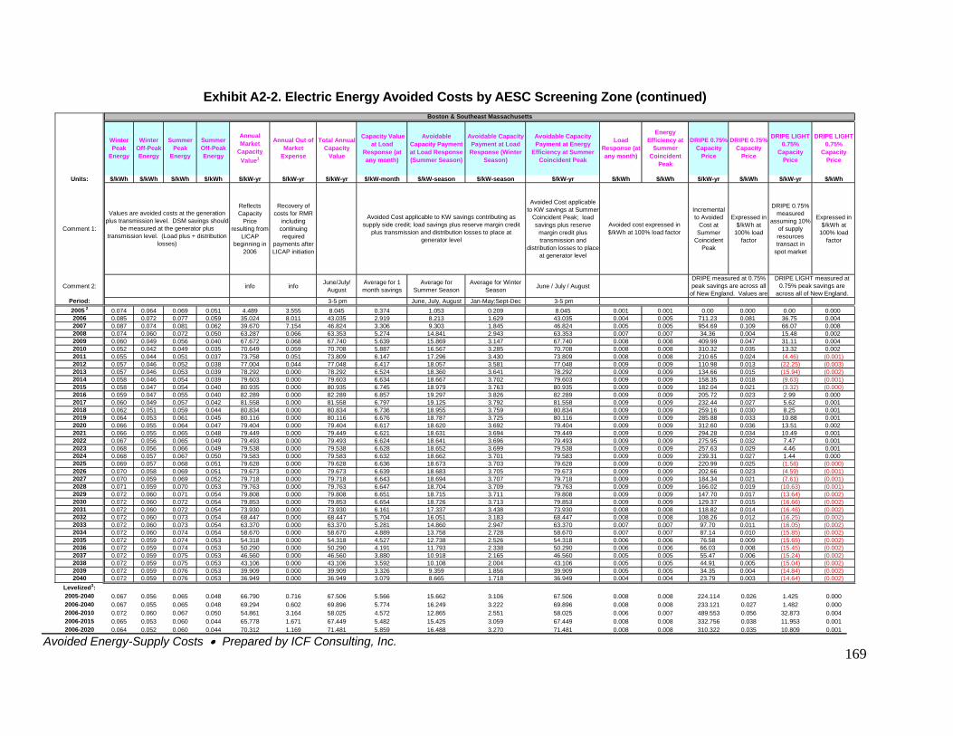
Avoided Energy-Supply Costs • Prepared by ICF Consulting, Inc.
169
Exhibit A2-2. Electric Energy Avoided Costs by AESC Screening Zone (continued)
Winter Peak
Energy
Winter Off-Peak Energy
Summer Peak
Energy
Summer Off-Peak Energy
Annual Market
Capacity Value1
Annual Out of Market
Expense
Total Annual Capacity
Value
Capacity Value at Load
Response (at any month)
Avoidable Capacity Payment at Load Response (Summer Season)
Avoidable Capacity Payment at Load Response (Winter
Season)
Avoidable Capacity Payment at Energy
Efficiency at Summer Coincident Peak
Load Response (at any month)
Energy Efficiency at
Summer Coincident
Peak
DRIPE 0.75% Capacity
Price
DRIPE 0.75% Capacity
Price
DRIPE LIGHT 0.75%
Capacity Price
DRIPE LIGHT 0.75%
Capacity Price
Units: $/kWh $/kWh $/kWh $/kWh $/kW-yr $/kW-yr $/kW-yr $/kW-month $/kW-season $/kW-season $/kW-yr $/kWh $/kWh $/kW-yr $/kWh $/kW-yr $/kWh
Comment 1:
Reflects Capacity
Price resulting from
LICAP beginning in
2006
Recovery of costs for RMR
including continuing required
payments after LICAP initiation
Avoided Cost applicable to KW savings at Summer
Coincident Peak; load savings plus reserve
margin credit plus transmission and
distribution losses to place at generator level
Incremental to Avoided
Cost at Summer
Coincident Peak
Expressed in $/kWh at
100% load factor
DRIPE 0.75% measured
assuming 10% of supply resources transact in
spot market
Expressed in $/kWh at
100% load factor
Comment 2: info info June/July/ August
Average for 1 month savings
Average for Summer Season
Average for Winter Season June / July / August
Period: 3-5 pm June, July, August Jan-May;Sept-Dec 3-5 pm2005 2 0.074 0.064 0.069 0.051 4.489 3.555 8.045 0.374 1.053 0.209 8.045 0.001 0.001 0.00 0.000 0.00 0.0002006 0.085 0.072 0.077 0.059 35.024 8.011 43.035 2.919 8.213 1.629 43.035 0.004 0.005 711.23 0.081 36.75 0.0042007 0.087 0.074 0.081 0.062 39.670 7.154 46.824 3.306 9.303 1.845 46.824 0.005 0.005 954.69 0.109 66.07 0.0082008 0.074 0.060 0.072 0.050 63.287 0.066 63.353 5.274 14.841 2.943 63.353 0.007 0.007 34.36 0.004 15.48 0.0022009 0.060 0.049 0.056 0.040 67.672 0.068 67.740 5.639 15.869 3.147 67.740 0.008 0.008 409.99 0.047 31.11 0.0042010 0.052 0.042 0.049 0.035 70.649 0.059 70.708 5.887 16.567 3.285 70.708 0.008 0.008 310.32 0.035 13.32 0.0022011 0.055 0.044 0.051 0.037 73.758 0.051 73.809 6.147 17.296 3.430 73.809 0.008 0.008 210.65 0.024 (4.46) (0.001)
(22.25) (0.003)(15.94) (0.002)(9.63) (0.001)(3.32) (0.000)2.99 0.000
(1.58) (0.000)(4.59) (0.001)(7.61) (0.001)
(10.63) (0.001)(13.64) (0.002)(16.66) (0.002)(16.46) (0.002)(16.25) (0.002)(16.05) (0.002)(15.85) (0.002)(15.65) (0.002)(15.45) (0.002)(15.24) (0.002)(15.04) (0.002)(14.84) (0.002)(14.64) (0.002)
2012 0.057 0.046 0.052 0.038 77.004 0.044 77.048 6.417 18.057 3.581 77.048 0.009 0.009 110.98 0.0132013 0.057 0.046 0.053 0.039 78.292 0.000 78.292 6.524 18.360 3.641 78.292 0.009 0.009 134.66 0.0152014 0.058 0.046 0.054 0.039 79.603 0.000 79.603 6.634 18.667 3.702 79.603 0.009 0.009 158.35 0.0182015 0.058 0.047 0.054 0.040 80.935 0.000 80.935 6.745 18.979 3.763 80.935 0.009 0.009 182.04 0.0212016 0.059 0.047 0.055 0.040 82.289 0.000 82.289 6.857 19.297 3.826 82.289 0.009 0.009 205.72 0.0232017 0.060 0.049 0.057 0.042 81.558 0.000 81.558 6.797 19.125 3.792 81.558 0.009 0.009 232.44 0.027 5.62 0.0012018 0.062 0.051 0.059 0.044 80.834 0.000 80.834 6.736 18.955 3.759 80.834 0.009 0.009 259.16 0.030 8.25 0.0012019 0.064 0.053 0.061 0.045 80.116 0.000 80.116 6.676 18.787 3.725 80.116 0.009 0.009 285.88 0.033 10.88 0.0012020 0.066 0.055 0.064 0.047 79.404 0.000 79.404 6.617 18.620 3.692 79.404 0.009 0.009 312.60 0.036 13.51 0.0022021 0.066 0.055 0.065 0.048 79.449 0.000 79.449 6.621 18.631 3.694 79.449 0.009 0.009 294.28 0.034 10.49 0.0012022 0.067 0.056 0.065 0.049 79.493 0.000 79.493 6.624 18.641 3.696 79.493 0.009 0.009 275.95 0.032 7.47 0.0012023 0.068 0.056 0.066 0.049 79.538 0.000 79.538 6.628 18.652 3.699 79.538 0.009 0.009 257.63 0.029 4.46 0.0012024 0.068 0.057 0.067 0.050 79.583 0.000 79.583 6.632 18.662 3.701 79.583 0.009 0.009 239.31 0.027 1.44 0.0002025 0.069 0.057 0.068 0.051 79.628 0.000 79.628 6.636 18.673 3.703 79.628 0.009 0.009 220.99 0.0252026 0.070 0.058 0.069 0.051 79.673 0.000 79.673 6.639 18.683 3.705 79.673 0.009 0.009 202.66 0.0232027 0.070 0.059 0.069 0.052 79.718 0.000 79.718 6.643 18.694 3.707 79.718 0.009 0.009 184.34 0.0212028 0.071 0.059 0.070 0.053 79.763 0.000 79.763 6.647 18.704 3.709 79.763 0.009 0.009 166.02 0.0192029 0.072 0.060 0.071 0.054 79.808 0.000 79.808 6.651 18.715 3.711 79.808 0.009 0.009 147.70 0.0172030 0.072 0.060 0.072 0.054 79.853 0.000 79.853 6.654 18.726 3.713 79.853 0.009 0.009 129.37 0.0152031 0.072 0.060 0.072 0.054 73.930 0.000 73.930 6.161 17.337 3.438 73.930 0.008 0.008 118.82 0.0142032 0.072 0.060 0.073 0.054 68.447 0.000 68.447 5.704 16.051 3.183 68.447 0.008 0.008 108.26 0.0122033 0.072 0.060 0.073 0.054 63.370 0.000 63.370 5.281 14.860 2.947 63.370 0.007 0.007 97.70 0.0112034 0.072 0.060 0.074 0.054 58.670 0.000 58.670 4.889 13.758 2.728 58.670 0.007 0.007 87.14 0.0102035 0.072 0.059 0.074 0.053 54.318 0.000 54.318 4.527 12.738 2.526 54.318 0.006 0.006 76.58 0.0092036 0.072 0.059 0.074 0.053 50.290 0.000 50.290 4.191 11.793 2.338 50.290 0.006 0.006 66.03 0.0082037 0.072 0.059 0.075 0.053 46.560 0.000 46.560 3.880 10.918 2.165 46.560 0.005 0.005 55.47 0.0062038 0.072 0.059 0.075 0.053 43.106 0.000 43.106 3.592 10.108 2.004 43.106 0.005 0.005 44.91 0.0052039 0.072 0.059 0.076 0.053 39.909 0.000 39.909 3.326 9.359 1.856 39.909 0.005 0.005 34.35 0.0042040 0.072 0.059 0.076 0.053 36.949 0.000 36.949 3.079 8.665 1.718 36.949 0.004 0.004 23.79 0.003
Levelized3: 2005-2040 0.067 0.056 0.065 0.048 66.790 0.716 67.506 5.566 15.662 3.106 67.506 0.008 0.008 224.114 0.026 1.425 0.0002006-2040 0.067 0.055 0.065 0.048 69.294 0.602 69.896 5.774 16.249 3.222 69.896 0.008 0.008 233.121 0.027 1.482 0.0002006-2010 0.072 0.060 0.067 0.050 54.861 3.164 58.025 4.572 12.865 2.551 58.025 0.006 0.007 489.553 0.056 32.873 0.0042006-2015 0.065 0.053 0.060 0.044 65.778 1.671 67.449 5.482 15.425 3.059 67.449 0.008 0.008 332.756 0.038 11.953 0.0012006-2020 0.064 0.052 0.060 0.044 70.312 1.169 71.481 5.859 16.488 3.270 71.481 0.008 0.008 310.322 0.035 10.809 0.001
Boston & Southeast Massachusetts
Values are avoided costs at the generation plus transmission level. DSM savings should
be measured at the generator plus transmission level. (Load plus + distribution
losses)
DRIPE measured at 0.75% peak savings are across all
of New England. Values are
Avoided cost expressed in $/kWh at 100% load factor
Avoided Cost applicable to KW savings contributing as supply side credit; load savings plus reserve margin credit
plus transmission and distribution losses to place at generator level
DRIPE LIGHT measured at 0.75% peak savings are
across all of New England.
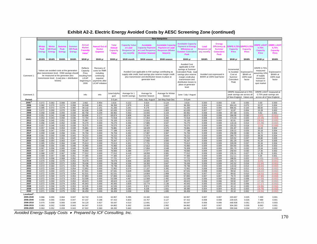
Avoided Energy-Supply Costs • Prepared by ICF Consulting, Inc.
170
Exhibit A2-2. Electric Energy Avoided Costs by AESC Screening Zone (continued)
Winter Peak
Energy
Winter Off-Peak Energy
Summer Peak
Energy
Summer Off-Peak Energy
Annual Market
Capacity Value1
Annual Out of Market
Expense
Total Annual
Capacity Value
Capacity Value at Load
Response (at any month)
Avoidable Capacity Payment at Load Response (Summer Season)
Avoidable Capacity Payment at Load Response (Winter
Season)
Avoidable Capacity Payment at Energy
Efficiency at Summer Coincident
Peak
Load Response (at any month)
Energy Efficiency at
Summer Coincident
Peak
DRIPE 0.75% Capacity
Price
DRIPE 0.75% Capacity
Price
DRIPE LIGHT 0.75%
Capacity Price
DRIPE LIGHT 0.75%
Capacity Price
Units: $/kWh $/kWh $/kWh $/kWh $/kW-yr $/kW-yr $/kW-yr $/kW-month $/kW-season $/kW-season $/kW-yr $/kWh $/kWh $/kW-yr $/kWh $/kW-yr $/kWh
Comment 1:
Reflects Capacity
Price resulting from
LICAP beginning in
2006
Recovery of costs for RMR
including continuing required
payments after LICAP initiation
Avoided Cost applicable to KW
savings at Summer Coincident Peak; load savings plus reserve
margin credit plus transmission and
distribution losses to place at generator
level
Incremental to Avoided
Cost at Summer
Coincident Peak
Expressed in $/kWh at
100% load factor
DRIPE 0.75% measured
assuming 10% of supply resources transact in
spot market
Expressed in $/kWh at
100% load factor
Comment 2: info info June/July/August
Average for 1 month savings
Average for Summer Season
Average for Winter Season June / July / August
Period: 3-5 pm June, July, August Jan-May;Sept-Dec 3-5 pm2005 2 0.072 0.063 0.066 0.049 2.662 0.954 3.616 0.222 0.624 0.124 3.616 0.000 0.000 0.00 0.000 0.00 0.0002006 0.082 0.070 0.074 0.058 34.548 1.801 36.350 2.879 8.102 1.607 36.350 0.004 0.004 654.43 0.075 32.57 0.0042007 0.085 0.072 0.079 0.060 39.132 2.151 41.283 3.261 9.176 1.820 41.283 0.004 0.005 906.91 0.104 88.60 0.0102008 0.072 0.059 0.070 0.050 62.436 0.199 62.635 5.203 14.641 2.903 62.635 0.007 0.007 32.87 0.004 15.28 0.0022009 0.058 0.048 0.055 0.039 66.758 0.204 66.962 5.563 15.655 3.104 66.962 0.008 0.008 357.68 0.041 9.62 0.0012010 0.051 0.041 0.048 0.034 69.696 0.177 69.874 5.808 16.344 3.241 69.874 0.008 0.008 266.06 0.030 (6.87) (0.001)
(23.35) (0.003)(39.84) (0.005)(21.08) (0.002)(2.33) (0.000)16.43 0.002
(0.65) (0.000)(6.65) (0.001)
(12.64) (0.001)(18.64) (0.002)(18.43) (0.002)(18.22) (0.002)(18.01) (0.002)(17.80) (0.002)(17.59) (0.002)(17.38) (0.002)(17.17) (0.002)(16.96) (0.002)(16.75) (0.002)(16.54) (0.002)
2011 0.053 0.043 0.050 0.036 72.764 0.154 72.918 6.064 17.063 3.384 72.918 0.008 0.008 174.43 0.0202012 0.056 0.045 0.051 0.038 75.967 0.133 76.100 6.331 17.814 3.532 76.100 0.009 0.009 82.81 0.0092013 0.056 0.045 0.052 0.038 76.270 0.000 76.270 6.356 17.885 3.547 76.270 0.009 0.009 119.16 0.0142014 0.057 0.046 0.053 0.039 76.575 0.000 76.575 6.381 17.957 3.561 76.575 0.009 0.009 155.52 0.0182015 0.057 0.046 0.053 0.039 76.881 0.000 76.881 6.407 18.029 3.575 76.881 0.009 0.009 191.87 0.0222016 0.058 0.047 0.054 0.039 77.188 0.000 77.188 6.432 18.101 3.589 77.188 0.009 0.009 228.22 0.026 35.18 0.0042017 0.059 0.048 0.056 0.041 76.704 0.000 76.704 6.392 17.987 3.567 76.704 0.009 0.009 258.99 0.030 36.72 0.0042018 0.061 0.050 0.058 0.043 76.222 0.000 76.222 6.352 17.874 3.544 76.222 0.009 0.009 289.75 0.033 38.26 0.0042019 0.063 0.052 0.061 0.045 75.743 0.000 75.743 6.312 17.762 3.522 75.743 0.009 0.009 320.52 0.037 39.80 0.0052020 0.065 0.054 0.063 0.047 75.267 0.000 75.267 6.272 17.650 3.500 75.267 0.009 0.009 351.29 0.040 41.34 0.0052021 0.065 0.054 0.064 0.048 75.613 0.000 75.613 6.301 17.731 3.516 75.613 0.009 0.009 328.09 0.037 35.34 0.0042022 0.066 0.055 0.065 0.048 75.960 0.000 75.960 6.330 17.813 3.532 75.960 0.009 0.009 304.90 0.035 29.34 0.0032023 0.067 0.056 0.065 0.049 76.309 0.000 76.309 6.359 17.894 3.548 76.309 0.009 0.009 281.70 0.032 23.34 0.0032024 0.067 0.056 0.066 0.050 76.660 0.000 76.660 6.388 17.977 3.565 76.660 0.009 0.009 258.50 0.030 17.35 0.0022025 0.068 0.057 0.067 0.050 77.012 0.000 77.012 6.418 18.059 3.581 77.012 0.009 0.009 235.31 0.027 11.35 0.0012026 0.069 0.057 0.068 0.051 77.365 0.000 77.365 6.447 18.142 3.597 77.365 0.009 0.009 212.11 0.024 5.35 0.0012027 0.070 0.058 0.069 0.052 77.721 0.000 77.721 6.477 18.225 3.614 77.721 0.009 0.009 188.91 0.0222028 0.070 0.058 0.070 0.053 78.078 0.000 78.078 6.506 18.309 3.631 78.078 0.009 0.009 165.72 0.0192029 0.071 0.059 0.071 0.053 78.436 0.000 78.436 6.536 18.393 3.647 78.436 0.009 0.009 142.52 0.0162030 0.072 0.060 0.071 0.054 78.796 0.000 78.796 6.566 18.478 3.664 78.796 0.009 0.009 119.32 0.0142031 0.072 0.059 0.072 0.054 72.952 0.000 72.952 6.079 17.107 3.392 72.952 0.008 0.008 109.42 0.0122032 0.072 0.059 0.072 0.054 67.541 0.000 67.541 5.628 15.838 3.141 67.541 0.008 0.008 99.52 0.0112033 0.072 0.059 0.073 0.054 62.531 0.000 62.531 5.211 14.664 2.908 62.531 0.007 0.007 89.62 0.0102034 0.072 0.059 0.073 0.053 57.893 0.000 57.893 4.824 13.576 2.692 57.893 0.007 0.007 79.72 0.0092035 0.072 0.059 0.073 0.053 53.599 0.000 53.599 4.467 12.569 2.492 53.599 0.006 0.006 69.82 0.0082036 0.072 0.059 0.074 0.053 49.623 0.000 49.623 4.135 11.637 2.307 49.623 0.006 0.006 59.92 0.0072037 0.072 0.058 0.074 0.053 45.943 0.000 45.943 3.829 10.774 2.136 45.943 0.005 0.005 50.02 0.0062038 0.071 0.058 0.075 0.053 42.535 0.000 42.535 3.545 9.974 1.978 42.535 0.005 0.005 40.12 0.0052039 0.071 0.058 0.075 0.052 39.380 0.000 39.380 3.282 9.235 1.831 39.380 0.004 0.004 30.22 0.0032040 0.071 0.058 0.075 0.052 36.459 0.000 36.459 3.038 8.550 1.695 36.459 0.004 0.004 20.32 0.002
Levelized3: 2005-2040 0.066 0.055 0.064 0.047 64.742 0.215 64.957 5.395 15.182 3.010 64.957 0.007 0.007 220.657 0.025 7.200 0.0012006-2040 0.066 0.055 0.064 0.047 67.237 0.186 67.422 5.603 15.767 3.127 67.422 0.008 0.008 229.525 0.026 7.489 0.0012006-2010 0.070 0.059 0.065 0.049 54.120 0.927 55.047 4.510 12.691 2.517 55.047 0.006 0.006 448.938 0.051 28.472 0.0032006-2015 0.063 0.052 0.059 0.043 64.347 0.515 64.862 5.362 15.089 2.992 64.862 0.007 0.007 304.283 0.035 8.063 0.0012006-2020 0.063 0.052 0.059 0.043 67.922 0.360 68.282 5.660 15.928 3.158 68.282 0.008 0.008 299.546 0.034 17.117 0.002
New Hampshire
Values are avoided costs at the generation plus transmission level. DSM savings should
be measured at the generator plus transmission level. (Load plus + distribution
losses)
Avoided cost expressed in $/kWh at 100% load factor
DRIPE measured at 0.75% peak savings are across all
of New England. Values are
DRIPE LIGHT measured at 0.75% peak savings are
across all of New England.
Avoided Cost applicable to KW savings contributing as supply side credit; load savings plus reserve margin credit
plus transmission and distribution losses to place at generator level
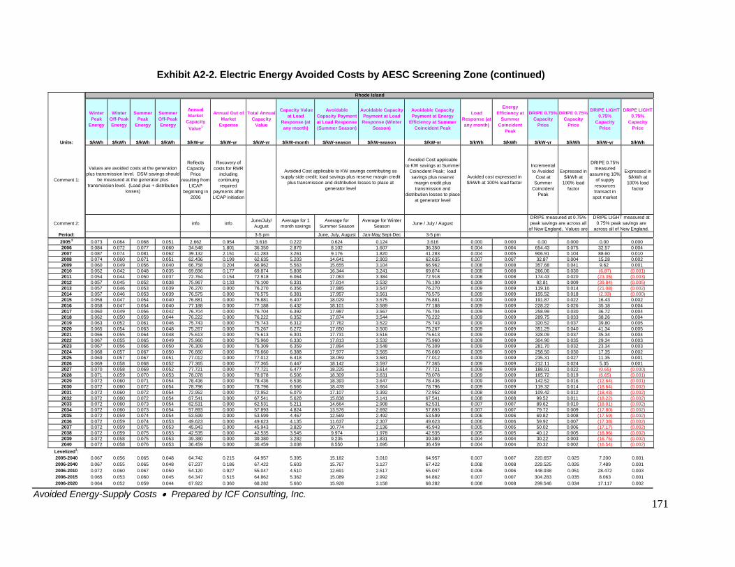
Avoided Energy-Supply Costs • Prepared by ICF Consulting, Inc.
171
Exhibit A2-2. Electric Energy Avoided Costs by AESC Screening Zone (continued)
Winter Peak
Energy
Winter Off-Peak Energy
Summer Peak
Energy
Summer Off-Peak Energy
Annual Market
Capacity Value1
Annual Out of Market
Expense
Total Annual Capacity
Value
Capacity Value at Load
Response (at any month)
Avoidable Capacity Payment at Load Response (Summer Season)
Avoidable Capacity Payment at Load Response (Winter
Season)
Avoidable Capacity Payment at Energy
Efficiency at Summer Coincident Peak
Load Response (at any month)
Energy Efficiency at
Summer Coincident
Peak
DRIPE 0.75% Capacity
Price
DRIPE 0.75% Capacity
Price
DRIPE LIGHT 0.75%
Capacity Price
DRIPE LIGHT 0.75%
Capacity Price
Units: $/kWh $/kWh $/kWh $/kWh $/kW-yr $/kW-yr $/kW-yr $/kW-month $/kW-season $/kW-season $/kW-yr $/kWh $/kWh $/kW-yr $/kWh $/kW-yr $/kWh
Comment 1:
Reflects Capacity
Price resulting from
LICAP beginning in
2006
Recovery of costs for RMR
including continuing required
payments after LICAP initiation
Avoided Cost applicable to KW savings at Summer
Coincident Peak; load savings plus reserve
margin credit plus transmission and
distribution losses to place at generator level
Incremental to Avoided
Cost at Summer
Coincident Peak
Expressed in $/kWh at
100% load factor
DRIPE 0.75% measured
assuming 10% of supply resources transact in
spot market
Expressed in $/kWh at
100% load factor
Comment 2: info info June/July/ August
Average for 1 month savings
Average for Summer Season
Average for Winter Season June / July / August
Period: 3-5 pm June, July, August Jan-May;Sept-Dec 3-5 pm2005 2 0.073 0.064 0.068 0.051 2.662 0.954 3.616 0.222 0.624 0.124 3.616 0.000 0.000 0.00 0.000 0.00 0.0002006 0.084 0.072 0.077 0.060 34.548 1.801 36.350 2.879 8.102 1.607 36.350 0.004 0.004 654.43 0.075 32.57 0.0042007 0.087 0.074 0.081 0.062 39.132 2.151 41.283 3.261 9.176 1.820 41.283 0.004 0.005 906.91 0.104 88.60 0.0102008 0.074 0.060 0.071 0.051 62.436 0.199 62.635 5.203 14.641 2.903 62.635 0.007 0.007 32.87 0.004 15.28 0.0022009 0.060 0.049 0.056 0.040 66.758 0.204 66.962 5.563 15.655 3.104 66.962 0.008 0.008 357.68 0.041 9.62 0.0012010 0.052 0.042 0.048 0.035 69.696 0.177 69.874 5.808 16.344 3.241 69.874 0.008 0.008 266.06 0.030 (6.87) (0.001)
(23.35) (0.003)(39.84) (0.005)(21.08) (0.002)(2.33) (0.000)16.43 0.002
(0.65) (0.000)(6.65) (0.001)(12.64) (0.001)(18.64) (0.002)(18.43) (0.002)(18.22) (0.002)(18.01) (0.002)(17.80) (0.002)(17.59) (0.002)(17.38) (0.002)(17.17) (0.002)(16.96) (0.002)(16.75) (0.002)(16.54) (0.002)
2011 0.054 0.044 0.050 0.037 72.764 0.154 72.918 6.064 17.063 3.384 72.918 0.008 0.008 174.43 0.0202012 0.057 0.045 0.052 0.038 75.967 0.133 76.100 6.331 17.814 3.532 76.100 0.009 0.009 82.81 0.0092013 0.057 0.046 0.053 0.039 76.270 0.000 76.270 6.356 17.885 3.547 76.270 0.009 0.009 119.16 0.0142014 0.057 0.046 0.053 0.039 76.575 0.000 76.575 6.381 17.957 3.561 76.575 0.009 0.009 155.52 0.0182015 0.058 0.047 0.054 0.040 76.881 0.000 76.881 6.407 18.029 3.575 76.881 0.009 0.009 191.87 0.0222016 0.058 0.047 0.054 0.040 77.188 0.000 77.188 6.432 18.101 3.589 77.188 0.009 0.009 228.22 0.026 35.18 0.0042017 0.060 0.049 0.056 0.042 76.704 0.000 76.704 6.392 17.987 3.567 76.704 0.009 0.009 258.99 0.030 36.72 0.0042018 0.062 0.050 0.059 0.044 76.222 0.000 76.222 6.352 17.874 3.544 76.222 0.009 0.009 289.75 0.033 38.26 0.0042019 0.063 0.052 0.061 0.046 75.743 0.000 75.743 6.312 17.762 3.522 75.743 0.009 0.009 320.52 0.037 39.80 0.0052020 0.065 0.054 0.063 0.048 75.267 0.000 75.267 6.272 17.650 3.500 75.267 0.009 0.009 351.29 0.040 41.34 0.0052021 0.066 0.055 0.064 0.048 75.613 0.000 75.613 6.301 17.731 3.516 75.613 0.009 0.009 328.09 0.037 35.34 0.0042022 0.067 0.055 0.065 0.049 75.960 0.000 75.960 6.330 17.813 3.532 75.960 0.009 0.009 304.90 0.035 29.34 0.0032023 0.067 0.056 0.066 0.050 76.309 0.000 76.309 6.359 17.894 3.548 76.309 0.009 0.009 281.70 0.032 23.34 0.0032024 0.068 0.057 0.067 0.050 76.660 0.000 76.660 6.388 17.977 3.565 76.660 0.009 0.009 258.50 0.030 17.35 0.0022025 0.069 0.057 0.067 0.051 77.012 0.000 77.012 6.418 18.059 3.581 77.012 0.009 0.009 235.31 0.027 11.35 0.0012026 0.069 0.058 0.068 0.052 77.365 0.000 77.365 6.447 18.142 3.597 77.365 0.009 0.009 212.11 0.024 5.35 0.0012027 0.070 0.058 0.069 0.052 77.721 0.000 77.721 6.477 18.225 3.614 77.721 0.009 0.009 188.91 0.0222028 0.071 0.059 0.070 0.053 78.078 0.000 78.078 6.506 18.309 3.631 78.078 0.009 0.009 165.72 0.0192029 0.072 0.060 0.071 0.054 78.436 0.000 78.436 6.536 18.393 3.647 78.436 0.009 0.009 142.52 0.0162030 0.072 0.060 0.072 0.054 78.796 0.000 78.796 6.566 18.478 3.664 78.796 0.009 0.009 119.32 0.0142031 0.072 0.060 0.072 0.054 72.952 0.000 72.952 6.079 17.107 3.392 72.952 0.008 0.008 109.42 0.0122032 0.072 0.060 0.072 0.054 67.541 0.000 67.541 5.628 15.838 3.141 67.541 0.008 0.008 99.52 0.0112033 0.072 0.060 0.073 0.054 62.531 0.000 62.531 5.211 14.664 2.908 62.531 0.007 0.007 89.62 0.0102034 0.072 0.060 0.073 0.054 57.893 0.000 57.893 4.824 13.576 2.692 57.893 0.007 0.007 79.72 0.0092035 0.072 0.059 0.074 0.054 53.599 0.000 53.599 4.467 12.569 2.492 53.599 0.006 0.006 69.82 0.0082036 0.072 0.059 0.074 0.053 49.623 0.000 49.623 4.135 11.637 2.307 49.623 0.006 0.006 59.92 0.0072037 0.072 0.059 0.075 0.053 45.943 0.000 45.943 3.829 10.774 2.136 45.943 0.005 0.005 50.02 0.0062038 0.072 0.059 0.075 0.053 42.535 0.000 42.535 3.545 9.974 1.978 42.535 0.005 0.005 40.12 0.0052039 0.072 0.058 0.075 0.053 39.380 0.000 39.380 3.282 9.235 1.831 39.380 0.004 0.004 30.22 0.0032040 0.072 0.058 0.076 0.053 36.459 0.000 36.459 3.038 8.550 1.695 36.459 0.004 0.004 20.32 0.002
Levelized3: 2005-2040 0.067 0.056 0.065 0.048 64.742 0.215 64.957 5.395 15.182 3.010 64.957 0.007 0.007 220.657 0.025 7.200 0.0012006-2040 0.067 0.055 0.065 0.048 67.237 0.186 67.422 5.603 15.767 3.127 67.422 0.008 0.008 229.525 0.026 7.489 0.0012006-2010 0.072 0.060 0.067 0.050 54.120 0.927 55.047 4.510 12.691 2.517 55.047 0.006 0.006 448.938 0.051 28.472 0.0032006-2015 0.065 0.053 0.060 0.045 64.347 0.515 64.862 5.362 15.089 2.992 64.862 0.007 0.007 304.283 0.035 8.063 0.0012006-2020 0.064 0.052 0.059 0.044 67.922 0.360 68.282 5.660 15.928 3.158 68.282 0.008 0.008 299.546 0.034 17.117 0.002
Rhode Island
Values are avoided costs at the generation plus transmission level. DSM savings should
be measured at the generator plus transmission level. (Load plus + distribution
losses)
Avoided cost expressed in $/kWh at 100% load factor
DRIPE measured at 0.75% peak savings are across all
of New England. Values are
DRIPE LIGHT measured at 0.75% peak savings are
across all of New England.
Avoided Cost applicable to KW savings contributing as supply side credit; load savings plus reserve margin credit
plus transmission and distribution losses to place at generator level
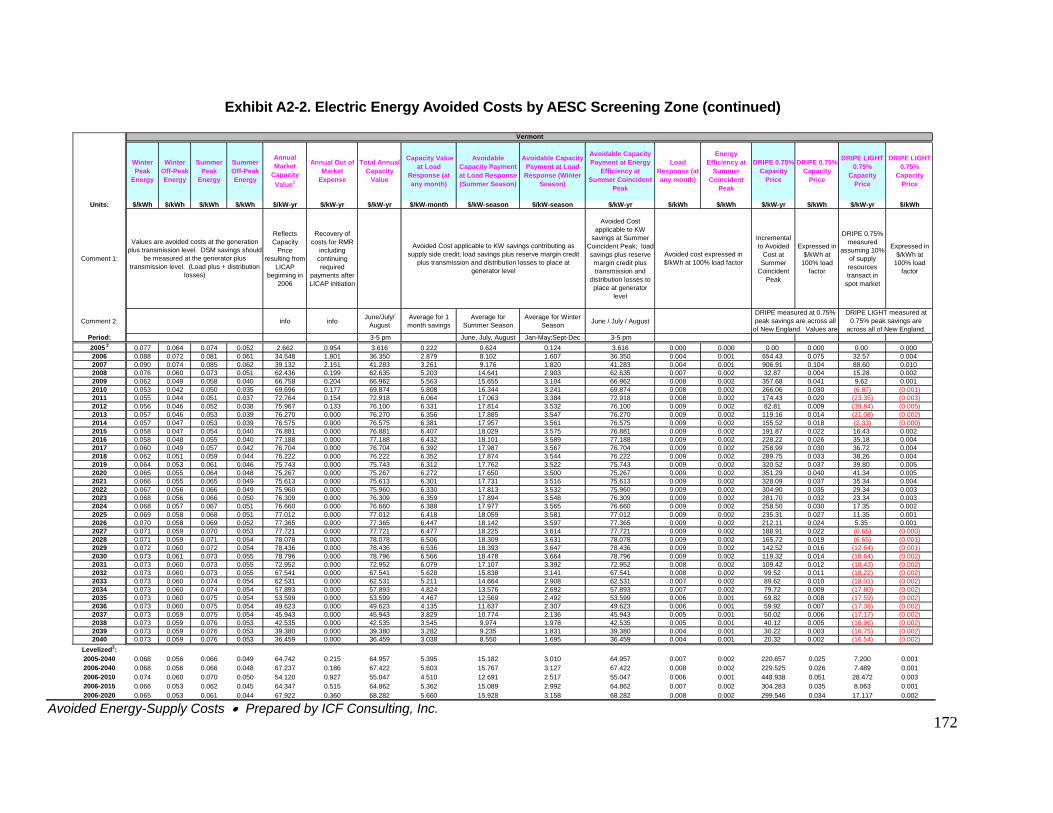
Avoided Energy-Supply Costs • Prepared by ICF Consulting, Inc.
172
Exhibit A2-2. Electric Energy Avoided Costs by AESC Screening Zone (continued)
Winter Peak
Energy
Winter Off-Peak Energy
Summer Peak
Energy
Summer Off-Peak Energy
Annual Market
Capacity Value1
Annual Out of Market
Expense
Total Annual Capacity
Value
Capacity Value at Load
Response (at any month)
Avoidable Capacity Payment at Load Response (Summer Season)
Avoidable Capacity Payment at Load Response (Winter
Season)
Avoidable Capacity Payment at Energy
Efficiency at Summer Coincident
Peak
Load Response (at any month)
Energy Efficiency at
Summer Coincident
Peak
DRIPE 0.75% Capacity
Price
DRIPE 0.75% Capacity
Price
DRIPE LIGHT 0.75%
Capacity Price
DRIPE LIGHT 0.75%
Capacity Price
Units: $/kWh $/kWh $/kWh $/kWh $/kW-yr $/kW-yr $/kW-yr $/kW-month $/kW-season $/kW-season $/kW-yr $/kWh $/kWh $/kW-yr $/kWh $/kW-yr $/kWh
Comment 1:
Reflects Capacity
Price resulting from
LICAP beginning in
2006
Recovery of costs for RMR
including continuing required
payments after LICAP initiation
Avoided Cost applicable to KW
savings at Summer Coincident Peak; load savings plus reserve
margin credit plus transmission and
distribution losses to place at generator
level
Incremental to Avoided
Cost at Summer
Coincident Peak
Expressed in $/kWh at
100% load factor
DRIPE 0.75% measured
assuming 10% of supply resources transact in
spot market
Expressed in $/kWh at
100% load factor
Comment 2: info info June/July/ August
Average for 1 month savings
Average for Summer Season
Average for Winter Season June / July / August
Period: 3-5 pm June, July, August Jan-May;Sept-Dec 3-5 pm2005 2 0.077 0.064 0.074 0.052 2.662 0.954 3.616 0.222 0.624 0.124 3.616 0.000 0.000 0.00 0.000 0.00 0.0002006 0.088 0.072 0.081 0.061 34.548 1.801 36.350 2.879 8.102 1.607 36.350 0.004 0.001 654.43 0.075 32.57 0.0042007 0.090 0.074 0.085 0.062 39.132 2.151 41.283 3.261 9.176 1.820 41.283 0.004 0.001 906.91 0.104 88.60 0.0102008 0.076 0.060 0.073 0.051 62.436 0.199 62.635 5.203 14.641 2.903 62.635 0.007 0.002 32.87 0.004 15.28 0.0022009 0.062 0.049 0.058 0.040 66.758 0.204 66.962 5.563 15.655 3.104 66.962 0.008 0.002 357.68 0.041 9.62 0.0012010 0.053 0.042 0.050 0.035 69.696 0.177 69.874 5.808 16.344 3.241 69.874 0.008 0.002 266.06 0.030 (6.87) (0.001)
(23.35) (0.003)(39.84) (0.005)(21.08) (0.002)(2.33) (0.000)16.43 0.002
(0.65) (0.000)(6.65) (0.001)(12.64) (0.001)(18.64) (0.002)(18.43) (0.002)(18.22) (0.002)(18.01) (0.002)(17.80) (0.002)(17.59) (0.002)(17.38) (0.002)(17.17) (0.002)(16.96) (0.002)(16.75) (0.002)(16.54) (0.002)
2011 0.055 0.044 0.051 0.037 72.764 0.154 72.918 6.064 17.063 3.384 72.918 0.008 0.002 174.43 0.0202012 0.056 0.046 0.052 0.038 75.967 0.133 76.100 6.331 17.814 3.532 76.100 0.009 0.002 82.81 0.0092013 0.057 0.046 0.053 0.039 76.270 0.000 76.270 6.356 17.885 3.547 76.270 0.009 0.002 119.16 0.0142014 0.057 0.047 0.053 0.039 76.575 0.000 76.575 6.381 17.957 3.561 76.575 0.009 0.002 155.52 0.0182015 0.058 0.047 0.054 0.040 76.881 0.000 76.881 6.407 18.029 3.575 76.881 0.009 0.002 191.87 0.0222016 0.058 0.048 0.055 0.040 77.188 0.000 77.188 6.432 18.101 3.589 77.188 0.009 0.002 228.22 0.026 35.18 0.0042017 0.060 0.049 0.057 0.042 76.704 0.000 76.704 6.392 17.987 3.567 76.704 0.009 0.002 258.99 0.030 36.72 0.0042018 0.062 0.051 0.059 0.044 76.222 0.000 76.222 6.352 17.874 3.544 76.222 0.009 0.002 289.75 0.033 38.26 0.0042019 0.064 0.053 0.061 0.046 75.743 0.000 75.743 6.312 17.762 3.522 75.743 0.009 0.002 320.52 0.037 39.80 0.0052020 0.065 0.055 0.064 0.048 75.267 0.000 75.267 6.272 17.650 3.500 75.267 0.009 0.002 351.29 0.040 41.34 0.0052021 0.066 0.055 0.065 0.049 75.613 0.000 75.613 6.301 17.731 3.516 75.613 0.009 0.002 328.09 0.037 35.34 0.0042022 0.067 0.056 0.066 0.049 75.960 0.000 75.960 6.330 17.813 3.532 75.960 0.009 0.002 304.90 0.035 29.34 0.0032023 0.068 0.056 0.066 0.050 76.309 0.000 76.309 6.359 17.894 3.548 76.309 0.009 0.002 281.70 0.032 23.34 0.0032024 0.068 0.057 0.067 0.051 76.660 0.000 76.660 6.388 17.977 3.565 76.660 0.009 0.002 258.50 0.030 17.35 0.0022025 0.069 0.058 0.068 0.051 77.012 0.000 77.012 6.418 18.059 3.581 77.012 0.009 0.002 235.31 0.027 11.35 0.0012026 0.070 0.058 0.069 0.052 77.365 0.000 77.365 6.447 18.142 3.597 77.365 0.009 0.002 212.11 0.024 5.35 0.0012027 0.071 0.059 0.070 0.053 77.721 0.000 77.721 6.477 18.225 3.614 77.721 0.009 0.002 188.91 0.0222028 0.071 0.059 0.071 0.054 78.078 0.000 78.078 6.506 18.309 3.631 78.078 0.009 0.002 165.72 0.0192029 0.072 0.060 0.072 0.054 78.436 0.000 78.436 6.536 18.393 3.647 78.436 0.009 0.002 142.52 0.0162030 0.073 0.061 0.073 0.055 78.796 0.000 78.796 6.566 18.478 3.664 78.796 0.009 0.002 119.32 0.0142031 0.073 0.060 0.073 0.055 72.952 0.000 72.952 6.079 17.107 3.392 72.952 0.008 0.002 109.42 0.0122032 0.073 0.060 0.073 0.055 67.541 0.000 67.541 5.628 15.838 3.141 67.541 0.008 0.002 99.52 0.0112033 0.073 0.060 0.074 0.054 62.531 0.000 62.531 5.211 14.664 2.908 62.531 0.007 0.002 89.62 0.0102034 0.073 0.060 0.074 0.054 57.893 0.000 57.893 4.824 13.576 2.692 57.893 0.007 0.002 79.72 0.0092035 0.073 0.060 0.075 0.054 53.599 0.000 53.599 4.467 12.569 2.492 53.599 0.006 0.001 69.82 0.0082036 0.073 0.060 0.075 0.054 49.623 0.000 49.623 4.135 11.637 2.307 49.623 0.006 0.001 59.92 0.0072037 0.073 0.059 0.075 0.054 45.943 0.000 45.943 3.829 10.774 2.136 45.943 0.005 0.001 50.02 0.0062038 0.073 0.059 0.076 0.053 42.535 0.000 42.535 3.545 9.974 1.978 42.535 0.005 0.001 40.12 0.0052039 0.073 0.059 0.076 0.053 39.380 0.000 39.380 3.282 9.235 1.831 39.380 0.004 0.001 30.22 0.0032040 0.073 0.059 0.076 0.053 36.459 0.000 36.459 3.038 8.550 1.695 36.459 0.004 0.001 20.32 0.002
Levelized3: 2005-2040 0.068 0.056 0.066 0.049 64.742 0.215 64.957 5.395 15.182 3.010 64.957 0.007 0.002 220.657 0.025 7.200 0.0012006-2040 0.068 0.056 0.066 0.048 67.237 0.186 67.422 5.603 15.767 3.127 67.422 0.008 0.002 229.525 0.026 7.489 0.0012006-2010 0.074 0.060 0.070 0.050 54.120 0.927 55.047 4.510 12.691 2.517 55.047 0.006 0.001 448.938 0.051 28.472 0.0032006-2015 0.066 0.053 0.062 0.045 64.347 0.515 64.862 5.362 15.089 2.992 64.862 0.007 0.002 304.283 0.035 8.063 0.0012006-2020 0.065 0.053 0.061 0.044 67.922 0.360 68.282 5.660 15.928 3.158 68.282 0.008 0.002 299.546 0.034 17.117 0.002
Vermont
Avoided cost expressed in $/kWh at 100% load factor
Values are avoided costs at the generation plus transmission level. DSM savings should
be measured at the generator plus transmission level. (Load plus + distribution
losses)
Avoided Cost applicable to KW savings contributing as supply side credit; load savings plus reserve margin credit
plus transmission and distribution losses to place at generator level
DRIPE measured at 0.75% peak savings are across all
of New England. Values are
DRIPE LIGHT measured at 0.75% peak savings are
across all of New England.
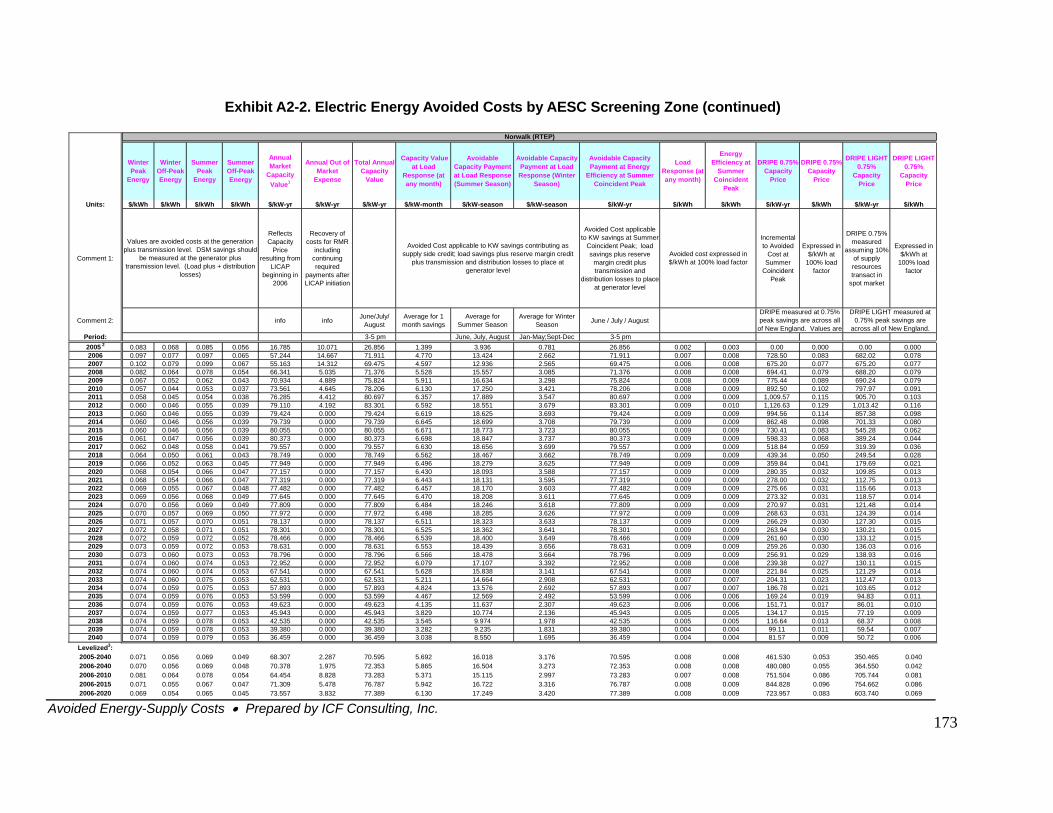
Avoided Energy-Supply Costs • Prepared by ICF Consulting, Inc.
173
Exhibit A2-2. Electric Energy Avoided Costs by AESC Screening Zone (continued)
Winter Peak
Energy
Winter Off-Peak Energy
Summer Peak
Energy
Summer Off-Peak Energy
Annual Market
Capacity Value1
Annual Out of Market
Expense
Total Annual Capacity
Value
Capacity Value at Load
Response (at any month)
Avoidable Capacity Payment at Load Response (Summer Season)
Avoidable Capacity Payment at Load Response (Winter
Season)
Avoidable Capacity Payment at Energy
Efficiency at Summer Coincident Peak
Load Response (at any month)
Energy Efficiency at
Summer Coincident
Peak
DRIPE 0.75% Capacity
Price
DRIPE 0.75% Capacity
Price
DRIPE LIGHT 0.75%
Capacity Price
DRIPE LIGHT 0.75%
Capacity Price
Units: $/kWh $/kWh $/kWh $/kWh $/kW-yr $/kW-yr $/kW-yr $/kW-month $/kW-season $/kW-season $/kW-yr $/kWh $/kWh $/kW-yr $/kWh $/kW-yr $/kWh
Comment 1:
Reflects Capacity
Price resulting from
LICAP beginning in
2006
Recovery of costs for RMR
including continuing required
payments after LICAP initiation
Avoided Cost applicable to KW savings at Summer
Coincident Peak; load savings plus reserve
margin credit plus transmission and
distribution losses to place at generator level
Incremental to Avoided
Cost at Summer
Coincident Peak
Expressed in $/kWh at
100% load factor
DRIPE 0.75% measured
assuming 10% of supply resources transact in
spot market
Expressed in $/kWh at
100% load factor
Comment 2: info info June/July/ August
Average for 1 month savings
Average for Summer Season
Average for Winter Season June / July / August
Period: 3-5 pm June, July, August Jan-May;Sept-Dec 3-5 pm2005 2 0.083 0.068 0.085 0.056 16.785 10.071 26.856 1.399 3.936 0.781 26.856 0.002 0.003 0.00 0.000 0.00 0.0002006 0.097 0.077 0.097 0.065 57.244 14.667 71.911 4.770 13.424 2.662 71.911 0.007 0.008 728.50 0.083 682.02 0.0782007 0.102 0.079 0.099 0.067 55.163 14.312 69.475 4.597 12.936 2.565 69.475 0.006 0.008 675.20 0.077 675.20 0.0772008 0.082 0.064 0.078 0.054 66.341 5.035 71.376 5.528 15.557 3.085 71.376 0.008 0.008 694.41 0.079 688.20 0.0792009 0.067 0.052 0.062 0.043 70.934 4.889 75.824 5.911 16.634 3.298 75.824 0.008 0.009 775.44 0.089 690.24 0.0792010 0.057 0.044 0.053 0.037 73.561 4.645 78.206 6.130 17.250 3.421 78.206 0.008 0.009 892.50 0.102 797.97 0.0912011 0.058 0.045 0.054 0.038 76.285 4.412 80.697 6.357 17.889 3.547 80.697 0.009 0.009 1,009.57 0.115 905.70 0.1032012 0.060 0.046 0.055 0.039 79.110 4.192 83.301 6.592 18.551 3.679 83.301 0.009 0.010 1,126.63 0.129 1,013.42 0.1162013 0.060 0.046 0.055 0.039 79.424 0.000 79.424 6.619 18.625 3.693 79.424 0.009 0.009 994.56 0.114 857.38 0.0982014 0.060 0.046 0.056 0.039 79.739 0.000 79.739 6.645 18.699 3.708 79.739 0.009 0.009 862.48 0.098 701.33 0.0802015 0.060 0.046 0.056 0.039 80.055 0.000 80.055 6.671 18.773 3.723 80.055 0.009 0.009 730.41 0.083 545.28 0.0622016 0.061 0.047 0.056 0.039 80.373 0.000 80.373 6.698 18.847 3.737 80.373 0.009 0.009 598.33 0.068 389.24 0.0442017 0.062 0.048 0.058 0.041 79.557 0.000 79.557 6.630 18.656 3.699 79.557 0.009 0.009 518.84 0.059 319.39 0.0362018 0.064 0.050 0.061 0.043 78.749 0.000 78.749 6.562 18.467 3.662 78.749 0.009 0.009 439.34 0.050 249.54 0.0282019 0.066 0.052 0.063 0.045 77.949 0.000 77.949 6.496 18.279 3.625 77.949 0.009 0.009 359.84 0.041 179.69 0.0212020 0.068 0.054 0.066 0.047 77.157 0.000 77.157 6.430 18.093 3.588 77.157 0.009 0.009 280.35 0.032 109.85 0.0132021 0.068 0.054 0.066 0.047 77.319 0.000 77.319 6.443 18.131 3.595 77.319 0.009 0.009 278.00 0.032 112.75 0.0132022 0.069 0.055 0.067 0.048 77.482 0.000 77.482 6.457 18.170 3.603 77.482 0.009 0.009 275.66 0.031 115.66 0.0132023 0.069 0.056 0.068 0.049 77.645 0.000 77.645 6.470 18.208 3.611 77.645 0.009 0.009 273.32 0.031 118.57 0.0142024 0.070 0.056 0.069 0.049 77.809 0.000 77.809 6.484 18.246 3.618 77.809 0.009 0.009 270.97 0.031 121.48 0.0142025 0.070 0.057 0.069 0.050 77.972 0.000 77.972 6.498 18.285 3.626 77.972 0.009 0.009 268.63 0.031 124.39 0.0142026 0.071 0.057 0.070 0.051 78.137 0.000 78.137 6.511 18.323 3.633 78.137 0.009 0.009 266.29 0.030 127.30 0.0152027 0.072 0.058 0.071 0.051 78.301 0.000 78.301 6.525 18.362 3.641 78.301 0.009 0.009 263.94 0.030 130.21 0.0152028 0.072 0.059 0.072 0.052 78.466 0.000 78.466 6.539 18.400 3.649 78.466 0.009 0.009 261.60 0.030 133.12 0.0152029 0.073 0.059 0.072 0.053 78.631 0.000 78.631 6.553 18.439 3.656 78.631 0.009 0.009 259.26 0.030 136.03 0.0162030 0.073 0.060 0.073 0.053 78.796 0.000 78.796 6.566 18.478 3.664 78.796 0.009 0.009 256.91 0.029 138.93 0.0162031 0.074 0.060 0.074 0.053 72.952 0.000 72.952 6.079 17.107 3.392 72.952 0.008 0.008 239.38 0.027 130.11 0.0152032 0.074 0.060 0.074 0.053 67.541 0.000 67.541 5.628 15.838 3.141 67.541 0.008 0.008 221.84 0.025 121.29 0.0142033 0.074 0.060 0.075 0.053 62.531 0.000 62.531 5.211 14.664 2.908 62.531 0.007 0.007 204.31 0.023 112.47 0.0132034 0.074 0.059 0.075 0.053 57.893 0.000 57.893 4.824 13.576 2.692 57.893 0.007 0.007 186.78 0.021 103.65 0.0122035 0.074 0.059 0.076 0.053 53.599 0.000 53.599 4.467 12.569 2.492 53.599 0.006 0.006 169.24 0.019 94.83 0.0112036 0.074 0.059 0.076 0.053 49.623 0.000 49.623 4.135 11.637 2.307 49.623 0.006 0.006 151.71 0.017 86.01 0.0102037 0.074 0.059 0.077 0.053 45.943 0.000 45.943 3.829 10.774 2.136 45.943 0.005 0.005 134.17 0.015 77.19 0.0092038 0.074 0.059 0.078 0.053 42.535 0.000 42.535 3.545 9.974 1.978 42.535 0.005 0.005 116.64 0.013 68.37 0.0082039 0.074 0.059 0.078 0.053 39.380 0.000 39.380 3.282 9.235 1.831 39.380 0.004 0.004 99.11 0.011 59.54 0.0072040 0.074 0.059 0.079 0.053 36.459 0.000 36.459 3.038 8.550 1.695 36.459 0.004 0.004 81.57 0.009 50.72 0.006
Levelized3: 2005-2040 0.071 0.056 0.069 0.049 68.307 2.287 70.595 5.692 16.018 3.176 70.595 0.008 0.008 461.530 0.053 350.465 0.0402006-2040 0.070 0.056 0.069 0.048 70.378 1.975 72.353 5.865 16.504 3.273 72.353 0.008 0.008 480.080 0.055 364.550 0.0422006-2010 0.081 0.064 0.078 0.054 64.454 8.828 73.283 5.371 15.115 2.997 73.283 0.007 0.008 751.504 0.086 705.744 0.0812006-2015 0.071 0.055 0.067 0.047 71.309 5.478 76.787 5.942 16.722 3.316 76.787 0.008 0.009 844.828 0.096 754.662 0.0862006-2020 0.069 0.054 0.065 0.045 73.557 3.832 77.389 6.130 17.249 3.420 77.389 0.008 0.009 723.957 0.083 603.740 0.069
Norwalk (RTEP)
Values are avoided costs at the generation plus transmission level. DSM savings should
be measured at the generator plus transmission level. (Load plus + distribution
losses)
Avoided Cost applicable to KW savings contributing as supply side credit; load savings plus reserve margin credit
plus transmission and distribution losses to place at generator level
Avoided cost expressed in $/kWh at 100% load factor
DRIPE measured at 0.75% peak savings are across all
of New England. Values are
DRIPE LIGHT measured at 0.75% peak savings are
across all of New England.

Avoided Energy-Supply Costs • Prepared by ICF Consulting, Inc.
174
Exhibit A2-2. Electric Energy Avoided Costs by AESC Screening Zone (continued)
Winter Peak
Energy
Winter Off-Peak Energy
Summer Peak
Energy
Summer Off-Peak Energy
Annual Market
Capacity Value1
Annual Out of Market
Expense
Total Annual Capacity
Value
Capacity Value at Load
Response (at any month)
Avoidable Capacity Payment at Load Response (Summer Season)
Avoidable Capacity Payment at Load Response (Winter
Season)
Avoidable Capacity Payment at Energy
Efficiency at Summer Coincident Peak
Load Response (at any month)
Energy Efficiency at
Summer Coincident
Peak
DRIPE 0.75% Capacity
Price
DRIPE 0.75% Capacity
Price
DRIPE LIGHT 0.75%
Capacity Price
DRIPE LIGHT 0.75%
Capacity Price
Units: $/kWh $/kWh $/kWh $/kWh $/kW-yr $/kW-yr $/kW-yr $/kW-month $/kW-season $/kW-season $/kW-yr $/kWh $/kWh $/kW-yr $/kWh $/kW-yr $/kWh
Comment 1:
Reflects Capacity
Price resulting from
LICAP beginning in
2006
Recovery of costs for RMR
including continuing required
payments after LICAP initiation
Avoided Cost applicable to KW savings at Summer
Coincident Peak; load savings plus reserve
margin credit plus transmission and
distribution losses to place at generator level
Incremental to Avoided
Cost at Summer
Coincident Peak
Expressed in $/kWh at
100% load factor
DRIPE 0.75% measured assuming
10% of supply
resources transact in
spot market
Expressed in $/kWh at
100% load factor
Comment 2: info info June/July/ August
Average for 1 month savings
Average for Summer Season
Average for Winter Season June / July / August
Period: 3-5 pm June, July, August Jan-May;Sept-Dec 3-5 pm2005 2 0.081 0.066 0.083 0.055 3.351 23.505 26.856 0.279 0.786 0.156 26.856 0.000 0.003 0.00 0.000 0.00 0.0002006 0.095 0.076 0.095 0.064 44.207 3.733 47.940 3.684 10.367 2.056 47.940 0.005 0.005 273.51 0.037 (14.21) (0.002)
(2.77) (2.77) (0.000)(34.01) (63.11) (0.007)337.05 (30.14) (0.003)
(141.89) (0.016)(25.03) (253.65) (0.029)
(206.08) (0.014) (365.40) (0.042)(145.52) (0.008) (321.89) (0.037)(84.97) (0.001) (278.38) (0.032)(24.42) 0.006 (234.87) (0.027)36.13 (191.36) (0.022)
(154.61) (0.018)(117.86) (0.013)(81.11) (0.009)(44.36) (0.005)(54.49) (0.006)(64.62) (0.007)(74.75) (0.009)(84.88) (0.010)(95.01) (0.011)(105.14) (0.012)(115.27) (0.013)(125.41) (0.014)(135.54) (0.015)(145.67) (0.017)(137.72) (0.016)(129.78) (0.015)(121.83) (0.014)(113.88) (0.013)
(1.28) (105.94) (0.012)(5.67) (97.99) (0.011)(10.06) (90.05) (0.010)(14.45) (82.10) (0.009)(18.84) (74.15) (0.008)(23.23) (66.21) (0.008)
2007 0.100 0.078 0.097 0.065 50.237 1.226 51.463 4.186 11.781 2.336 51.463 0.006 0.006 0.0062008 0.080 0.063 0.077 0.053 66.341 0.000 66.341 5.528 15.557 3.085 66.341 0.008 0.008 0.0042009 0.065 0.051 0.061 0.042 70.934 0.000 70.934 5.911 16.634 3.298 70.934 0.008 0.008 0.0472010 0.056 0.044 0.052 0.036 73.561 0.000 73.561 6.130 17.250 3.421 73.561 0.008 0.008 156.01 0.0262011 0.057 0.045 0.053 0.038 76.285 0.000 76.285 6.357 17.889 3.547 76.285 0.009 0.009 0.0062012 0.059 0.046 0.054 0.039 79.110 0.000 79.110 6.592 18.551 3.679 79.110 0.009 0.0092013 0.059 0.047 0.054 0.039 79.424 0.000 79.424 6.619 18.625 3.693 79.424 0.009 0.0092014 0.059 0.047 0.055 0.040 79.739 0.000 79.739 6.645 18.699 3.708 79.739 0.009 0.0092015 0.060 0.047 0.055 0.040 80.055 0.000 80.055 6.671 18.773 3.723 80.055 0.009 0.0092016 0.060 0.047 0.056 0.040 80.373 0.000 80.373 6.698 18.847 3.737 80.373 0.009 0.009 0.0132017 0.061 0.049 0.058 0.042 79.557 0.000 79.557 6.630 18.656 3.699 79.557 0.009 0.009 73.89 0.0182018 0.063 0.051 0.060 0.044 78.749 0.000 78.749 6.562 18.467 3.662 78.749 0.009 0.009 111.65 0.0222019 0.065 0.053 0.063 0.046 77.949 0.000 77.949 6.496 18.279 3.625 77.949 0.009 0.009 149.42 0.0262020 0.067 0.055 0.065 0.048 77.157 0.000 77.157 6.430 18.093 3.588 77.157 0.009 0.009 187.18 0.0302021 0.067 0.055 0.066 0.048 77.319 0.000 77.319 6.443 18.131 3.595 77.319 0.009 0.009 170.53 0.0282022 0.068 0.056 0.066 0.049 77.482 0.000 77.482 6.457 18.170 3.603 77.482 0.009 0.009 153.88 0.0262023 0.069 0.056 0.067 0.049 77.645 0.000 77.645 6.470 18.208 3.611 77.645 0.009 0.009 137.23 0.0252024 0.069 0.057 0.068 0.050 77.809 0.000 77.809 6.484 18.246 3.618 77.809 0.009 0.009 120.57 0.0232025 0.070 0.057 0.069 0.051 77.972 0.000 77.972 6.498 18.285 3.626 77.972 0.009 0.009 103.92 0.0212026 0.070 0.058 0.069 0.051 78.137 0.000 78.137 6.511 18.323 3.633 78.137 0.009 0.009 87.27 0.0192027 0.071 0.059 0.070 0.052 78.301 0.000 78.301 6.525 18.362 3.641 78.301 0.009 0.009 70.62 0.0172028 0.072 0.059 0.071 0.052 78.466 0.000 78.466 6.539 18.400 3.649 78.466 0.009 0.009 53.97 0.0152029 0.072 0.060 0.072 0.053 78.631 0.000 78.631 6.553 18.439 3.656 78.631 0.009 0.009 37.31 0.0132030 0.073 0.060 0.072 0.054 78.796 0.000 78.796 6.566 18.478 3.664 78.796 0.009 0.009 20.66 0.0112031 0.073 0.060 0.073 0.054 72.952 0.000 72.952 6.079 17.107 3.392 72.952 0.008 0.008 16.27 0.0102032 0.073 0.060 0.073 0.054 67.541 0.000 67.541 5.628 15.838 3.141 67.541 0.008 0.008 11.88 0.0092033 0.073 0.060 0.074 0.054 62.531 0.000 62.531 5.211 14.664 2.908 62.531 0.007 0.007 7.50 0.0082034 0.073 0.060 0.075 0.054 57.893 0.000 57.893 4.824 13.576 2.692 57.893 0.007 0.007 3.11 0.0072035 0.073 0.060 0.075 0.054 53.599 0.000 53.599 4.467 12.569 2.492 53.599 0.006 0.006 0.0062036 0.073 0.060 0.076 0.053 49.623 0.000 49.623 4.135 11.637 2.307 49.623 0.006 0.006 0.0052037 0.074 0.059 0.076 0.053 45.943 0.000 45.943 3.829 10.774 2.136 45.943 0.005 0.005 0.0042038 0.074 0.059 0.077 0.053 42.535 0.000 42.535 3.545 9.974 1.978 42.535 0.005 0.005 0.0032039 0.074 0.059 0.077 0.053 39.380 0.000 39.380 3.282 9.235 1.831 39.380 0.004 0.004 0.0022040 0.074 0.059 0.078 0.053 36.459 0.000 36.459 3.038 8.550 1.695 36.459 0.004 0.004 0.002
Levelized3: 2005-2040 0.070 0.056 0.069 0.049 67.112 1.095 68.207 5.593 15.738 3.121 68.207 0.008 0.008 51.439 0.014 -121.550 -0.0142006-2040 0.070 0.056 0.068 0.049 69.674 0.194 69.869 5.806 16.339 3.240 69.869 0.008 0.008 53.507 0.014 -126.435 -0.0142006-2010 0.079 0.063 0.077 0.053 60.736 1.027 61.763 5.061 14.243 2.824 61.763 0.007 0.007 145.560 0.024 -49.293 -0.0062006-2015 0.070 0.055 0.066 0.046 69.357 0.539 69.896 5.780 16.264 3.225 69.896 0.008 0.008 30.046 0.011 -164.235 -0.0192006-2020 0.068 0.054 0.064 0.045 72.191 0.377 72.568 6.016 16.929 3.357 72.568 0.008 0.008 54.110 0.014 -150.744 -0.017
Values are avoided costs at the generation plus transmission level. DSM savings should
be measured at the generator plus transmission level. (Load plus + distribution
losses)
Avoided Cost applicable to KW savings contributing as supply side credit; load savings plus reserve margin credit
plus transmission and distribution losses to place at generator level
Avoided cost expressed in $/kWh at 100% load factor
DRIPE measured at 0.75% peak savings are across all
of New England. Values are
DRIPE LIGHT measured at 0.75% peak savings are
across all of New England.
Southwest Connecticut (RTEP)
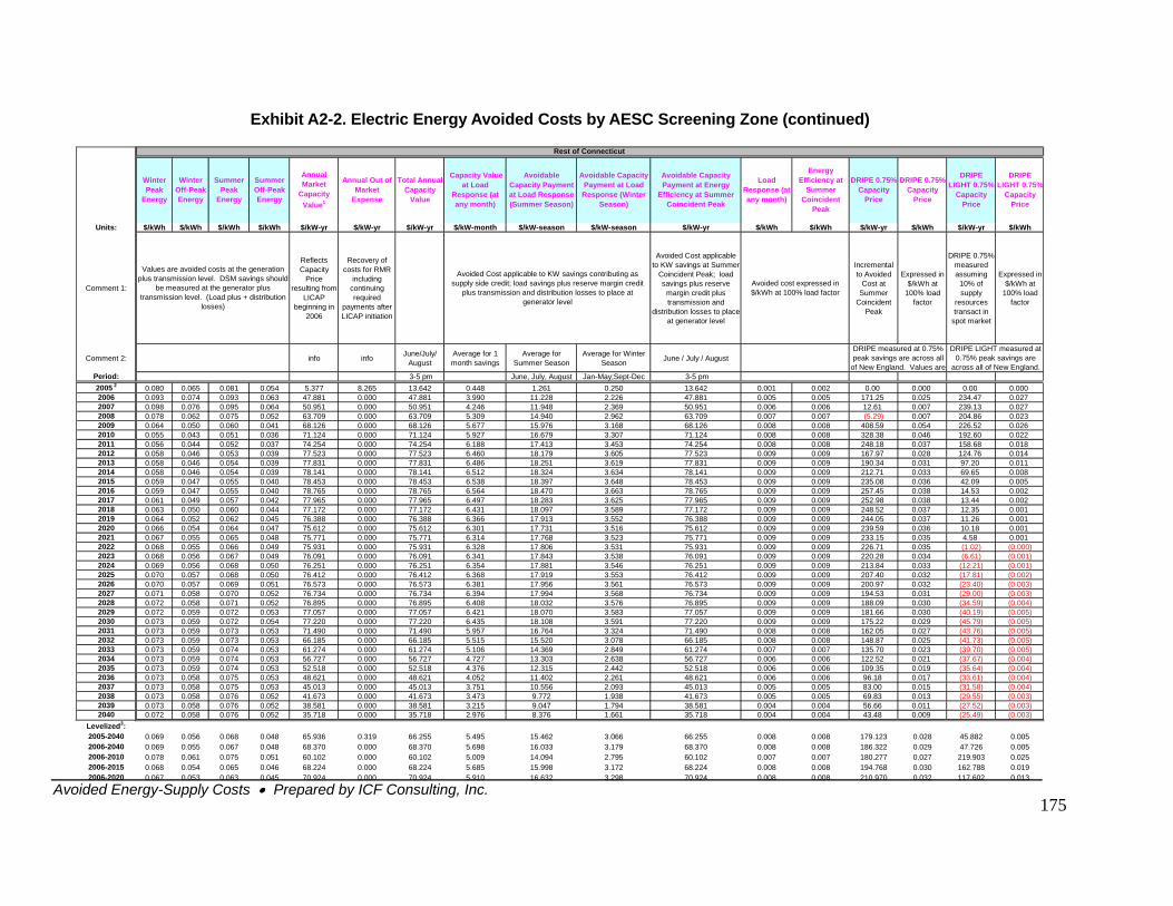
Avoided Energy-Supply Costs • Prepared by ICF Consulting, Inc.
175
Exhibit A2-2. Electric Energy Avoided Costs by AESC Screening Zone (continued)
Winter Peak
Energy
Winter Off-Peak Energy
Summer Peak
Energy
Summer Off-Peak Energy
Annual Market
Capacity Value1
Annual Out of Market
Expense
Total Annual Capacity
Value
Capacity Value at Load
Response (at any month)
Avoidable Capacity Payment at Load Response (Summer Season)
Avoidable Capacity Payment at Load Response (Winter
Season)
Avoidable Capacity Payment at Energy
Efficiency at Summer Coincident Peak
Load Response (at any month)
Energy Efficiency at
Summer Coincident
Peak
DRIPE 0.75% Capacity
Price
DRIPE 0.75% Capacity
Price
DRIPE LIGHT 0.75%
Capacity Price
DRIPE LIGHT 0.75%
Capacity Price
Units: $/kWh $/kWh $/kWh $/kWh $/kW-yr $/kW-yr $/kW-yr $/kW-month $/kW-season $/kW-season $/kW-yr $/kWh $/kWh $/kW-yr $/kWh $/kW-yr $/kWh
Comment 1:
Reflects Capacity
Price resulting from
LICAP beginning in
2006
Recovery of costs for RMR
including continuing required
payments after LICAP initiation
Avoided Cost applicable to KW savings at Summer
Coincident Peak; load savings plus reserve
margin credit plus transmission and
distribution losses to place at generator level
Incremental to Avoided
Cost at Summer
Coincident Peak
Expressed in $/kWh at
100% load factor
DRIPE 0.75% measured assuming
10% of supply
resources transact in
spot market
Expressed in $/kWh at
100% load factor
Comment 2: info info June/July/ August
Average for 1 month savings
Average for Summer Season
Average for Winter Season June / July / August
Period: 3-5 pm June, July, August Jan-May;Sept-Dec 3-5 pm2005 2 0.080 0.065 0.081 0.054 5.377 8.265 13.642 0.448 1.261 0.250 13.642 0.001 0.002 0.00 0.000 0.00 0.0002006 0.093 0.074 0.093 0.063 47.881 0.000 47.881 3.990 11.228 2.226 47.881 0.005 0.005 171.25 0.025 234.47 0.0272007 0.098 0.076 0.095 0.064 50.951 0.000 50.951 4.246 11.948 2.369 50.951 0.006 0.006 12.61 0.007 239.13 0.0272008 0.078 0.062 0.075 0.052 63.709 0.000 63.709 5.309 14.940 2.962 63.709 0.007 0.007 (5.29)
408.59
(1.02) (0.000)(6.61) (0.001)
(12.21) (0.001)(17.81) (0.002)(23.40) (0.003)(29.00) (0.003)(34.59) (0.004)(40.19) (0.005)(45.79) (0.005)(43.76) (0.005)(41.73) (0.005)(39.70) (0.005)(37.67) (0.004)(35.64) (0.004)(33.61) (0.004)(31.58) (0.004)(29.55) (0.003)(27.52) (0.003)(25.49) (0.003)
0.007 204.86 0.0232009 0.064 0.050 0.060 0.041 68.126 0.000 68.126 5.677 15.976 3.168 68.126 0.008 0.008 0.054 226.52 0.0262010 0.055 0.043 0.051 0.036 71.124 0.000 71.124 5.927 16.679 3.307 71.124 0.008 0.008 328.38 0.046 192.60 0.0222011 0.056 0.044 0.052 0.037 74.254 0.000 74.254 6.188 17.413 3.453 74.254 0.008 0.008 248.18 0.037 158.68 0.0182012 0.058 0.046 0.053 0.039 77.523 0.000 77.523 6.460 18.179 3.605 77.523 0.009 0.009 167.97 0.028 124.76 0.0142013 0.058 0.046 0.054 0.039 77.831 0.000 77.831 6.486 18.251 3.619 77.831 0.009 0.009 190.34 0.031 97.20 0.0112014 0.058 0.046 0.054 0.039 78.141 0.000 78.141 6.512 18.324 3.634 78.141 0.009 0.009 212.71 0.033 69.65 0.0082015 0.059 0.047 0.055 0.040 78.453 0.000 78.453 6.538 18.397 3.648 78.453 0.009 0.009 235.08 0.036 42.09 0.0052016 0.059 0.047 0.055 0.040 78.765 0.000 78.765 6.564 18.470 3.663 78.765 0.009 0.009 257.45 0.038 14.53 0.0022017 0.061 0.049 0.057 0.042 77.965 0.000 77.965 6.497 18.283 3.625 77.965 0.009 0.009 252.98 0.038 13.44 0.0022018 0.063 0.050 0.060 0.044 77.172 0.000 77.172 6.431 18.097 3.589 77.172 0.009 0.009 248.52 0.037 12.35 0.0012019 0.064 0.052 0.062 0.045 76.388 0.000 76.388 6.366 17.913 3.552 76.388 0.009 0.009 244.05 0.037 11.26 0.0012020 0.066 0.054 0.064 0.047 75.612 0.000 75.612 6.301 17.731 3.516 75.612 0.009 0.009 239.59 0.036 10.18 0.0012021 0.067 0.055 0.065 0.048 75.771 0.000 75.771 6.314 17.768 3.523 75.771 0.009 0.009 233.15 0.035 4.58 0.0012022 0.068 0.055 0.066 0.049 75.931 0.000 75.931 6.328 17.806 3.531 75.931 0.009 0.009 226.71 0.0352023 0.068 0.056 0.067 0.049 76.091 0.000 76.091 6.341 17.843 3.538 76.091 0.009 0.009 220.28 0.0342024 0.069 0.056 0.068 0.050 76.251 0.000 76.251 6.354 17.881 3.546 76.251 0.009 0.009 213.84 0.0332025 0.070 0.057 0.068 0.050 76.412 0.000 76.412 6.368 17.919 3.553 76.412 0.009 0.009 207.40 0.0322026 0.070 0.057 0.069 0.051 76.573 0.000 76.573 6.381 17.956 3.561 76.573 0.009 0.009 200.97 0.0322027 0.071 0.058 0.070 0.052 76.734 0.000 76.734 6.394 17.994 3.568 76.734 0.009 0.009 194.53 0.0312028 0.072 0.058 0.071 0.052 76.895 0.000 76.895 6.408 18.032 3.576 76.895 0.009 0.009 188.09 0.0302029 0.072 0.059 0.072 0.053 77.057 0.000 77.057 6.421 18.070 3.583 77.057 0.009 0.009 181.66 0.0302030 0.073 0.059 0.072 0.054 77.220 0.000 77.220 6.435 18.108 3.591 77.220 0.009 0.009 175.22 0.0292031 0.073 0.059 0.073 0.053 71.490 0.000 71.490 5.957 16.764 3.324 71.490 0.008 0.008 162.05 0.0272032 0.073 0.059 0.073 0.053 66.185 0.000 66.185 5.515 15.520 3.078 66.185 0.008 0.008 148.87 0.0252033 0.073 0.059 0.074 0.053 61.274 0.000 61.274 5.106 14.369 2.849 61.274 0.007 0.007 135.70 0.0232034 0.073 0.059 0.074 0.053 56.727 0.000 56.727 4.727 13.303 2.638 56.727 0.006 0.006 122.52 0.0212035 0.073 0.059 0.074 0.053 52.518 0.000 52.518 4.376 12.315 2.442 52.518 0.006 0.006 109.35 0.0192036 0.073 0.058 0.075 0.053 48.621 0.000 48.621 4.052 11.402 2.261 48.621 0.006 0.006 96.18 0.0172037 0.073 0.058 0.075 0.053 45.013 0.000 45.013 3.751 10.556 2.093 45.013 0.005 0.005 83.00 0.0152038 0.073 0.058 0.076 0.052 41.673 0.000 41.673 3.473 9.772 1.938 41.673 0.005 0.005 69.83 0.0132039 0.073 0.058 0.076 0.052 38.581 0.000 38.581 3.215 9.047 1.794 38.581 0.004 0.004 56.66 0.0112040 0.072 0.058 0.076 0.052 35.718 0.000 35.718 2.976 8.376 1.661 35.718 0.004 0.004 43.48 0.009
Levelized3: 2005-2040 0.069 0.056 0.068 0.048 65.936 0.319 66.255 5.495 15.462 3.066 66.255 0.008 0.008 179.123 0.028 45.882 0.0052006-2040 0.069 0.055 0.067 0.048 68.370 0.000 68.370 5.698 16.033 3.179 68.370 0.008 0.008 186.322 0.029 47.726 0.0052006-2010 0.078 0.061 0.075 0.051 60.102 0.000 60.102 5.009 14.094 2.795 60.102 0.007 0.007 180.277 0.027 219.903 0.0252006-2015 0.068 0.054 0.065 0.046 68.224 0.000 68.224 5.685 15.998 3.172 68.224 0.008 0.008 194.768 0.030 162.788 0.0192006-2020 0.067 0.053 0.063 0.045 70.924 0.000 70.924 5.910 16.632 3.298 70.924 0.008 0.008 210.970 0.032 117.602 0.013
Rest of Connecticut
DRIPE LIGHT measured at 0.75% peak savings are
across all of New England.
Values are avoided costs at the generation plus transmission level. DSM savings should
be measured at the generator plus transmission level. (Load plus + distribution
losses)
Avoided Cost applicable to KW savings contributing as supply side credit; load savings plus reserve margin credit
plus transmission and distribution losses to place at generator level
Avoided cost expressed in $/kWh at 100% load factor
DRIPE measured at 0.75% peak savings are across all
of New England. Values are
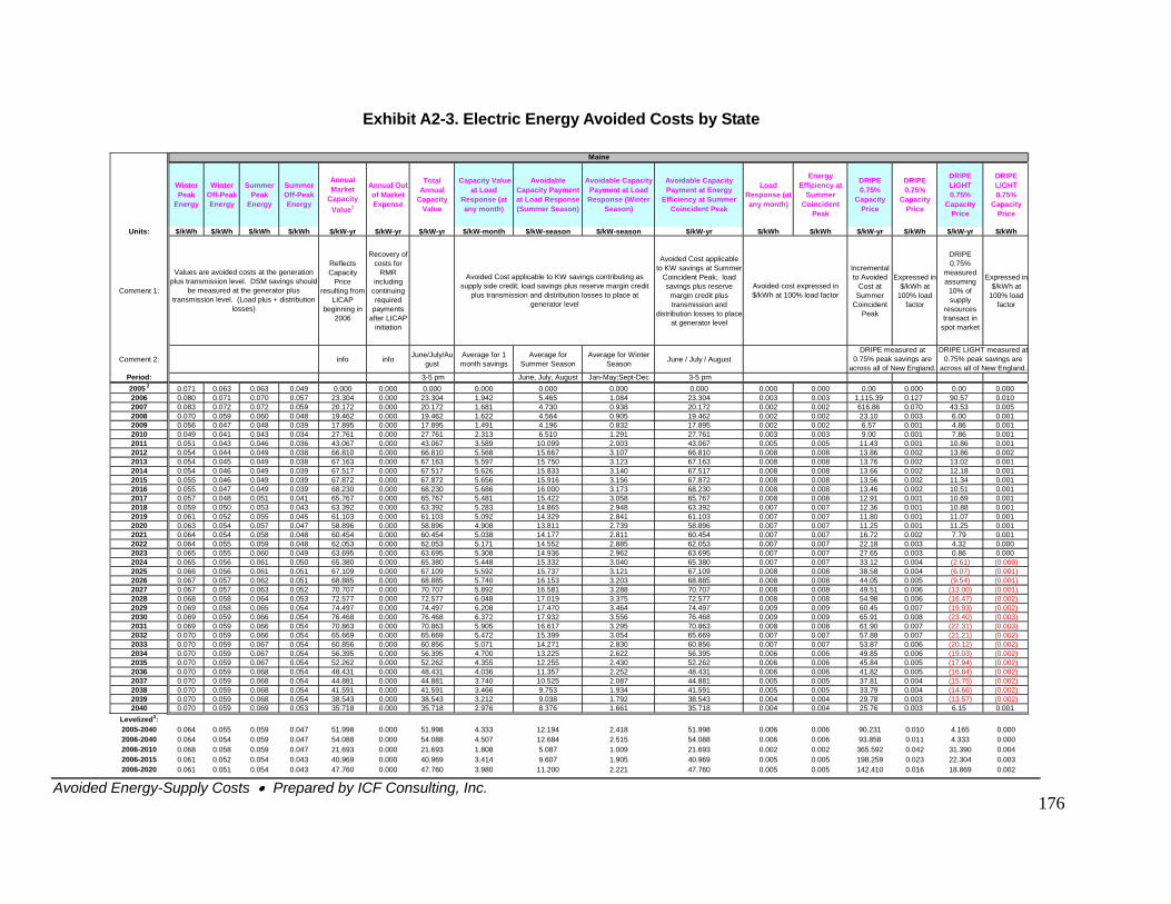
Avoided Energy-Supply Costs • Prepared by ICF Consulting, Inc.
176
Exhibit A2-3. Electric Energy Avoided Costs by State
Winter Peak
Energy
Winter Off-Peak Energy
Summer Peak
Energy
Summer Off-Peak Energy
Annual Market
Capacity Value1
Annual Out of Market Expense
Total Annual
Capacity Value
Capacity Value at Load
Response (at any month)
Avoidable Capacity Payment at Load Response (Summer Season)
Avoidable Capacity Payment at Load Response (Winter
Season)
Avoidable Capacity Payment at Energy
Efficiency at Summer Coincident Peak
Load Response (at any month)
Energy Efficiency at
Summer Coincident
Peak
DRIPE 0.75%
Capacity Price
DRIPE 0.75%
Capacity Price
DRIPE LIGHT 0.75%
Capacity Price
DRIPE LIGHT 0.75%
Capacity Price
Units: $/kWh $/kWh $/kWh $/kWh $/kW-yr $/kW-yr $/kW-yr $/kW-month $/kW-season $/kW-season $/kW-yr $/kWh $/kWh $/kW-yr $/kWh $/kW-yr $/kWh
Comment 1:
Reflects Capacity
Price resulting from
LICAP beginning in
2006
Recovery of costs for
RMR including
continuing required
payments after LICAP
initiation
Avoided Cost applicable to KW savings at Summer
Coincident Peak; load savings plus reserve
margin credit plus transmission and
distribution losses to place at generator level
Incremental to Avoided
Cost at Summer
Coincident Peak
Expressed in $/kWh at
100% load factor
DRIPE 0.75%
measured assuming
10% of supply
resources transact in
spot market
Expressed in $/kWh at
100% load factor
Comment 2: info info June/July/August
Average for 1 month savings
Average for Summer Season
Average for Winter Season June / July / August
Period: 3-5 pm June, July, August Jan-May;Sept-Dec 3-5 pm2005 2 0.071 0.063 0.063 0.049 0.000 0.000 0.000 0.000 0.000 0.000 0.000 0.000 0.000 0.00 0.000 0.00 0.0002006 0.080 0.071 0.070 0.057 23.304 0.000 23.304 1.942 5.465 1.084 23.304 0.003 0.003 1,115.39 0.127 90.57 0.0102007 0.083 0.072 0.072 0.059 20.172 0.000 20.172 1.681 4.730 0.938 20.172 0.002 0.002 616.86 0.070 43.53 0.0052008 0.070 0.059 0.060 0.048 19.462 0.000 19.462 1.622 4.564 0.905 19.462 0.002 0.002 23.10 0.003 6.00 0.0012009 0.056 0.047 0.048 0.039 17.895 0.000 17.895 1.491 4.196 0.832 17.895 0.002 0.002 6.57 0.001 4.86 0.0012010 0.049 0.041 0.043 0.034 27.761 0.000 27.761 2.313 6.510 1.291 27.761 0.003 0.003 9.00 0.001 7.86 0.0012011 0.051 0.043 0.046 0.036 43.067 0.000 43.067 3.589 10.099 2.003 43.067 0.005 0.005 11.43 0.001 10.86 0.0012012 0.054 0.044 0.049 0.038 66.810 0.000 66.810 5.568 15.667 3.107 66.810 0.008 0.008 13.86 0.002 13.86 0.0022013 0.054 0.045 0.049 0.038 67.163 0.000 67.163 5.597 15.750 3.123 67.163 0.008 0.008 13.76 0.002 13.02 0.0012014 0.054 0.046 0.049 0.039 67.517 0.000 67.517 5.626 15.833 3.140 67.517 0.008 0.008 13.66 0.002 12.18 0.0012015 0.055 0.046 0.049 0.039 67.872 0.000 67.872 5.656 15.916 3.156 67.872 0.008 0.008 13.56 0.002 11.34 0.0012016 0.055 0.047 0.049 0.039 68.230 0.000 68.230 5.686 16.000 3.173 68.230 0.008 0.008 13.46 0.002 10.51 0.0012017 0.057 0.048 0.051 0.041 65.767 0.000 65.767 5.481 15.422 3.058 65.767 0.008 0.008 12.91 0.001 10.69 0.0012018 0.059 0.050 0.053 0.043 63.392 0.000 63.392 5.283 14.865 2.948 63.392 0.007 0.007 12.36 0.001 10.88 0.0012019 0.061 0.052 0.055 0.045 61.103 0.000 61.103 5.092 14.329 2.841 61.103 0.007 0.007 11.80 0.001 11.07 0.0012020 0.063 0.054 0.057 0.047 58.896 0.000 58.896 4.908 13.811 2.739 58.896 0.007 0.007 11.25 0.001 11.25 0.0012021 0.064 0.054 0.058 0.048 60.454 0.000 60.454 5.038 14.177 2.811 60.454 0.007 0.007 16.72 0.002 7.79 0.0012022 0.064 0.055 0.059 0.048 62.053 0.000 62.053 5.171 14.552 2.885 62.053 0.007 0.007 22.18 0.003 4.32 0.0002023 0.065 0.055 0.060 0.049 63.695 0.000 63.695 5.308 14.936 2.962 63.695 0.007 0.007 27.65 0.003 0.86 0.0002024 0.065 0.056 0.061 0.050 65.380 0.000 65.380 5.448 15.332 3.040 65.380 0.007 0.007 33.12 0.004 (2.61) (0.000)
(6.07) (0.001)(9.54) (0.001)(13.00) (0.001)(16.47) (0.002)(19.93) (0.002)(23.40) (0.003)(22.31) (0.003)(21.21) (0.002)(20.12) (0.002)(19.03) (0.002)(17.94) (0.002)(16.84) (0.002)(15.75) (0.002)(14.66) (0.002)(13.57) (0.002)6.15 0.001
2025 0.066 0.056 0.061 0.051 67.109 0.000 67.109 5.592 15.737 3.121 67.109 0.008 0.008 38.58 0.0042026 0.067 0.057 0.062 0.051 68.885 0.000 68.885 5.740 16.153 3.203 68.885 0.008 0.008 44.05 0.0052027 0.067 0.057 0.063 0.052 70.707 0.000 70.707 5.892 16.581 3.288 70.707 0.008 0.008 49.51 0.0062028 0.068 0.058 0.064 0.053 72.577 0.000 72.577 6.048 17.019 3.375 72.577 0.008 0.008 54.98 0.0062029 0.069 0.058 0.065 0.054 74.497 0.000 74.497 6.208 17.470 3.464 74.497 0.009 0.009 60.45 0.0072030 0.069 0.059 0.066 0.054 76.468 0.000 76.468 6.372 17.932 3.556 76.468 0.009 0.009 65.91 0.0082031 0.069 0.059 0.066 0.054 70.863 0.000 70.863 5.905 16.617 3.295 70.863 0.008 0.008 61.90 0.0072032 0.070 0.059 0.066 0.054 65.669 0.000 65.669 5.472 15.399 3.054 65.669 0.007 0.007 57.88 0.0072033 0.070 0.059 0.067 0.054 60.856 0.000 60.856 5.071 14.271 2.830 60.856 0.007 0.007 53.87 0.0062034 0.070 0.059 0.067 0.054 56.395 0.000 56.395 4.700 13.225 2.622 56.395 0.006 0.006 49.85 0.0062035 0.070 0.059 0.067 0.054 52.262 0.000 52.262 4.355 12.255 2.430 52.262 0.006 0.006 45.84 0.0052036 0.070 0.059 0.068 0.054 48.431 0.000 48.431 4.036 11.357 2.252 48.431 0.006 0.006 41.82 0.0052037 0.070 0.059 0.068 0.054 44.881 0.000 44.881 3.740 10.525 2.087 44.881 0.005 0.005 37.81 0.0042038 0.070 0.059 0.068 0.054 41.591 0.000 41.591 3.466 9.753 1.934 41.591 0.005 0.005 33.79 0.0042039 0.070 0.059 0.068 0.054 38.543 0.000 38.543 3.212 9.038 1.792 38.543 0.004 0.004 29.78 0.0032040 0.070 0.059 0.069 0.053 35.718 0.000 35.718 2.976 8.376 1.661 35.718 0.004 0.004 25.76 0.003
Levelized3: 2005-2040 0.064 0.055 0.059 0.047 51.998 0.000 51.998 4.333 12.194 2.418 51.998 0.006 0.006 90.231 0.010 4.165 0.0002006-2040 0.064 0.054 0.059 0.047 54.088 0.000 54.088 4.507 12.684 2.515 54.088 0.006 0.006 93.858 0.011 4.333 0.0002006-2010 0.068 0.058 0.059 0.047 21.693 0.000 21.693 1.808 5.087 1.009 21.693 0.002 0.002 365.592 0.042 31.390 0.0042006-2015 0.061 0.052 0.054 0.043 40.969 0.000 40.969 3.414 9.607 1.905 40.969 0.005 0.005 198.259 0.023 22.304 0.0032006-2020 0.061 0.051 0.054 0.043 47.760 0.000 47.760 3.980 11.200 2.221 47.760 0.005 0.005 142.410 0.016 18.869 0.002
Avoided Cost applicable to KW savings contributing as supply side credit; load savings plus reserve margin credit
plus transmission and distribution losses to place at generator level
Values are avoided costs at the generation plus transmission level. DSM savings should
be measured at the generator plus transmission level. (Load plus + distribution
losses)
Avoided cost expressed in $/kWh at 100% load factor
Maine
DRIPE measured at 0.75% peak savings are
across all of New England.
DRIPE LIGHT measured at 0.75% peak savings are
across all of New England.
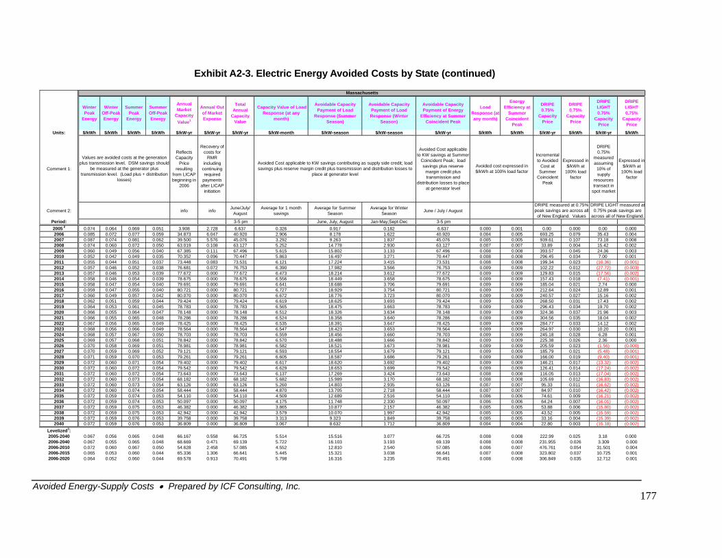
Avoided Energy-Supply Costs • Prepared by ICF Consulting, Inc.
177
Exhibit A2-3. Electric Energy Avoided Costs by State (continued)
Winter Peak
Energy
Winter Off-Peak Energy
Summer Peak
Energy
Summer Off-Peak Energy
Annual Market
Capacity Value1
Annual Out of Market Expense
Total Annual
Capacity Value
Capacity Value of Load Response (at any
month)
Avoidable Capacity Payment of Load
Response (Summer Season)
Avoidable Capacity Payment of Load Response (Winter
Season)
Avoidable Capacity Payment of Energy
Efficiency at Summer Coincident Peak
Load Response (at any month)
Energy Efficiency at
Summer Coincident
Peak
DRIPE 0.75%
Capacity Price
DRIPE 0.75%
Capacity Price
DRIPE LIGHT 0.75%
Capacity Price
DRIPE LIGHT 0.75%
Capacity Price
Units: $/kWh $/kWh $/kWh $/kWh $/kW-yr $/kW-yr $/kW-yr $/kW-month $/kW-season $/kW-season $/kW-yr $/kWh $/kWh $/kW-yr $/kWh $/kW-yr $/kWh
Comment 1:
Reflects Capacity
Price resulting
from LICAP beginning in
2006
Recovery of costs for
RMR including
continuing required
payments after LICAP
initiation
Avoided Cost applicable to KW savings at Summer
Coincident Peak; load savings plus reserve
margin credit plus transmission and
distribution losses to place at generator level
Incremental to Avoided
Cost at Summer
Coincident Peak
Expressed in $/kWh at
100% load factor
DRIPE 0.75%
measured assuming
10% of supply
resources transact in
spot market
Expressed in $/kWh at
100% load factor
Comment 2: info info June/July/ August
Average for 1 month savings
Average for Summer Season
Average for Winter Season June / July / August
Period: 3-5 pm June, July, August Jan-May;Sept-Dec 3-5 pm2005 2 0.074 0.064 0.069 0.051 3.908 2.728 6.637 0.326 0.917 0.182 6.637 0.000 0.001 0.00 0.000 0.00 0.0002006 0.085 0.072 0.077 0.059 34.873 6.047 40.920 2.906 8.178 1.622 40.920 0.004 0.005 693.25 0.079 35.43 0.0042007 0.087 0.074 0.081 0.062 39.500 5.576 45.076 3.292 9.263 1.837 45.076 0.005 0.005 939.61 0.107 73.18 0.0082008 0.074 0.060 0.072 0.050 63.019 0.108 63.127 5.252 14.778 2.930 63.127 0.007 0.007 33.89 0.004 15.42 0.0022009 0.060 0.049 0.056 0.040 67.385 0.111 67.496 5.615 15.802 3.133 67.496 0.008 0.008 393.57 0.045 24.36 0.0032010 0.052 0.042 0.049 0.035 70.352 0.096 70.447 5.863 16.497 3.271 70.447 0.008 0.008 296.45 0.034 7.00 0.0012011 0.055 0.044 0.051 0.037 73.448 0.083 73.531 6.121 17.224 3.415 73.531 0.008 0.008 199.34 0.023 (10.36) (0.001)
(27.72) (0.003)(17.56) (0.002)(7.41) (0.001)2.74 0.000
(1.56) (0.000)(5.48) (0.001)(9.40) (0.001)(13.32) (0.002)(17.24) (0.002)(17.04) (0.002)(16.83) (0.002)(16.62) (0.002)(16.42) (0.002)(16.21) (0.002)(16.01) (0.002)(15.80) (0.002)(15.59) (0.002)(15.39) (0.002)(15.18) (0.002)
2012 0.057 0.046 0.052 0.038 76.681 0.072 76.753 6.390 17.982 3.566 76.753 0.009 0.009 102.22 0.0122013 0.057 0.046 0.053 0.039 77.672 0.000 77.672 6.473 18.214 3.612 77.672 0.009 0.009 129.83 0.0152014 0.058 0.046 0.054 0.039 78.675 0.000 78.675 6.556 18.449 3.658 78.675 0.009 0.009 157.43 0.0182015 0.058 0.047 0.054 0.040 79.691 0.000 79.691 6.641 18.688 3.706 79.691 0.009 0.009 185.04 0.0212016 0.059 0.047 0.055 0.040 80.721 0.000 80.721 6.727 18.929 3.754 80.721 0.009 0.009 212.64 0.024 12.89 0.0012017 0.060 0.049 0.057 0.042 80.070 0.000 80.070 6.672 18.776 3.723 80.070 0.009 0.009 240.57 0.027 15.16 0.0022018 0.062 0.051 0.059 0.044 79.424 0.000 79.424 6.619 18.625 3.693 79.424 0.009 0.009 268.50 0.031 17.43 0.0022019 0.064 0.053 0.061 0.045 78.783 0.000 78.783 6.565 18.475 3.663 78.783 0.009 0.009 296.43 0.034 19.70 0.0022020 0.066 0.055 0.064 0.047 78.148 0.000 78.148 6.512 18.326 3.634 78.148 0.009 0.009 324.36 0.037 21.96 0.0032021 0.066 0.055 0.065 0.048 78.286 0.000 78.286 6.524 18.358 3.640 78.286 0.009 0.009 304.56 0.035 18.04 0.0022022 0.067 0.056 0.065 0.049 78.425 0.000 78.425 6.535 18.391 3.647 78.425 0.009 0.009 284.77 0.033 14.12 0.0022023 0.068 0.056 0.066 0.049 78.564 0.000 78.564 6.547 18.423 3.653 78.564 0.009 0.009 264.97 0.030 10.20 0.0012024 0.068 0.057 0.067 0.050 78.703 0.000 78.703 6.559 18.456 3.660 78.703 0.009 0.009 245.18 0.028 6.28 0.0012025 0.069 0.057 0.068 0.051 78.842 0.000 78.842 6.570 18.488 3.666 78.842 0.009 0.009 225.38 0.026 2.36 0.0002026 0.070 0.058 0.069 0.051 78.981 0.000 78.981 6.582 18.521 3.673 78.981 0.009 0.009 205.59 0.0232027 0.070 0.059 0.069 0.052 79.121 0.000 79.121 6.593 18.554 3.679 79.121 0.009 0.009 185.79 0.0212028 0.071 0.059 0.070 0.053 79.261 0.000 79.261 6.605 18.587 3.686 79.261 0.009 0.009 166.00 0.0192029 0.072 0.060 0.071 0.054 79.402 0.000 79.402 6.617 18.620 3.692 79.402 0.009 0.009 146.21 0.0172030 0.072 0.060 0.072 0.054 79.542 0.000 79.542 6.629 18.653 3.699 79.542 0.009 0.009 126.41 0.0142031 0.072 0.060 0.072 0.054 73.643 0.000 73.643 6.137 17.269 3.424 73.643 0.008 0.008 116.05 0.0132032 0.072 0.060 0.073 0.054 68.182 0.000 68.182 5.682 15.989 3.170 68.182 0.008 0.008 105.69 0.0122033 0.072 0.060 0.073 0.054 63.126 0.000 63.126 5.260 14.803 2.935 63.126 0.007 0.007 95.33 0.0112034 0.072 0.060 0.074 0.054 58.444 0.000 58.444 4.870 13.705 2.718 58.444 0.007 0.007 84.97 0.0102035 0.072 0.059 0.074 0.053 54.110 0.000 54.110 4.509 12.689 2.516 54.110 0.006 0.006 74.61 0.0092036 0.072 0.059 0.074 0.053 50.097 0.000 50.097 4.175 11.748 2.330 50.097 0.006 0.006 64.24 0.0072037 0.072 0.059 0.075 0.053 46.382 0.000 46.382 3.865 10.877 2.157 46.382 0.005 0.005 53.88 0.0062038 0.072 0.059 0.075 0.053 42.942 0.000 42.942 3.579 10.070 1.997 42.942 0.005 0.005 43.52 0.0052039 0.072 0.059 0.076 0.053 39.758 0.000 39.758 3.313 9.323 1.849 39.758 0.005 0.005 33.16 0.0042040 0.072 0.059 0.076 0.053 36.809 0.000 36.809 3.067 8.632 1.712 36.809 0.004 0.004 22.80 0.003
Levelized3: 2005-2040 0.067 0.056 0.065 0.048 66.167 0.558 66.725 5.514 15.516 3.077 66.725 0.008 0.008 222.99 0.025 3.18 0.0002006-2040 0.067 0.055 0.065 0.048 68.669 0.471 69.139 5.722 16.103 3.193 69.139 0.008 0.008 231.955 0.026 3.309 0.0002006-2010 0.072 0.060 0.067 0.050 54.628 2.458 57.085 4.552 12.810 2.540 57.085 0.006 0.007 476.761 0.054 31.501 0.0042006-2015 0.065 0.053 0.060 0.044 65.336 1.306 66.641 5.445 15.321 3.038 66.641 0.007 0.008 323.802 0.037 10.725 0.0012006-2020 0.064 0.052 0.060 0.044 69.578 0.913 70.491 5.798 16.316 3.235 70.491 0.008 0.008 306.849 0.035 12.712 0.001
Massachusetts
Avoided Cost applicable to KW savings contributing as supply side credit; load savings plus reserve margin credit plus transmission and distribution losses to
place at generator level
DRIPE LIGHT measured at 0.75% peak savings are
across all of New England.
Values are avoided costs at the generation plus transmission level. DSM savings should
be measured at the generator plus transmission level. (Load plus + distribution
losses)
Avoided cost expressed in $/kWh at 100% load factor
DRIPE measured at 0.75% peak savings are across all
of New England. Values
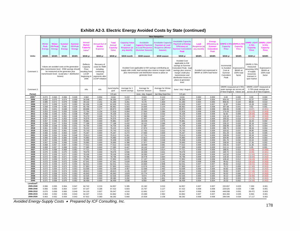
Avoided Energy-Supply Costs • Prepared by ICF Consulting, Inc.
178
Exhibit A2-3. Electric Energy Avoided Costs by State (continued)
Winter Peak
Energy
Winter Off-Peak Energy
Summer Peak
Energy
Summer Off-Peak Energy
Annual Market
Capacity Value1
Annual Out of Market
Expense
Total Annual
Capacity Value
Capacity Value at Load
Response (at any month)
Avoidable Capacity Payment at Load Response (Summer Season)
Avoidable Capacity Payment at Load Response (Winter
Season)
Avoidable Capacity Payment at Energy
Efficiency at Summer Coincident
Peak
Load Response (at any month)
Energy Efficiency at
Summer Coincident
Peak
DRIPE 0.75% Capacity
Price
DRIPE 0.75% Capacity
Price
DRIPE LIGHT 0.75%
Capacity Price
DRIPE LIGHT 0.75%
Capacity Price
Units: $/kWh $/kWh $/kWh $/kWh $/kW-yr $/kW-yr $/kW-yr $/kW-month $/kW-season $/kW-season $/kW-yr $/kWh $/kWh $/kW-yr $/kWh $/kW-yr $/kWh
Comment 1:
Reflects Capacity
Price resulting from
LICAP beginning in
2006
Recovery of costs for RMR
including continuing required
payments after LICAP initiation
Avoided Cost applicable to KW
savings at Summer Coincident Peak; load savings plus reserve
margin credit plus transmission and
distribution losses to place at generator
level
Incremental to Avoided
Cost at Summer
Coincident Peak
Expressed in $/kWh at
100% load factor
DRIPE 0.75% measured
assuming 10% of supply resources transact in
spot market
Expressed in $/kWh at
100% load factor
Comment 2: info info June/July/August
Average for 1 month savings
Average for Summer Season
Average for Winter Season June / July / August
Period: 3-5 pm June, July, August Jan-May;Sept-Dec 3-5 pm2005 2 0.072 0.063 0.066 0.049 2.662 0.954 3.616 0.222 0.624 0.124 3.616 0.000 0.000 0.00 0.000 0.00 0.0002006 0.082 0.070 0.074 0.058 34.548 1.801 36.350 2.879 8.102 1.607 36.350 0.004 0.004 654.43 0.075 32.57 0.0042007 0.085 0.072 0.079 0.060 39.132 2.151 41.283 3.261 9.176 1.820 41.283 0.004 0.005 906.91 0.104 88.60 0.0102008 0.072 0.059 0.070 0.050 62.436 0.199 62.635 5.203 14.641 2.903 62.635 0.007 0.007 32.87 0.004 15.28 0.0022009 0.058 0.048 0.055 0.039 66.758 0.204 66.962 5.563 15.655 3.104 66.962 0.008 0.008 357.68 0.041 9.62 0.0012010 0.051 0.041 0.048 0.034 69.696 0.177 69.874 5.808 16.344 3.241 69.874 0.008 0.008 266.06 0.030 (6.87) (0.001)
(23.35) (0.003)(39.84) (0.005)(21.08) (0.002)(2.33) (0.000)16.43 0.002
(0.65) (0.000)(6.65) (0.001)(12.64) (0.001)(18.64) (0.002)(18.43) (0.002)(18.22) (0.002)(18.01) (0.002)(17.80) (0.002)(17.59) (0.002)(17.38) (0.002)(17.17) (0.002)(16.96) (0.002)(16.75) (0.002)(16.54) (0.002)
2011 0.053 0.043 0.050 0.036 72.764 0.154 72.918 6.064 17.063 3.384 72.918 0.008 0.008 174.43 0.0202012 0.056 0.045 0.051 0.038 75.967 0.133 76.100 6.331 17.814 3.532 76.100 0.009 0.009 82.81 0.0092013 0.056 0.045 0.052 0.038 76.270 0.000 76.270 6.356 17.885 3.547 76.270 0.009 0.009 119.16 0.0142014 0.057 0.046 0.053 0.039 76.575 0.000 76.575 6.381 17.957 3.561 76.575 0.009 0.009 155.52 0.0182015 0.057 0.046 0.053 0.039 76.881 0.000 76.881 6.407 18.029 3.575 76.881 0.009 0.009 191.87 0.0222016 0.058 0.047 0.054 0.039 77.188 0.000 77.188 6.432 18.101 3.589 77.188 0.009 0.009 228.22 0.026 35.18 0.0042017 0.059 0.048 0.056 0.041 76.704 0.000 76.704 6.392 17.987 3.567 76.704 0.009 0.009 258.99 0.030 36.72 0.0042018 0.061 0.050 0.058 0.043 76.222 0.000 76.222 6.352 17.874 3.544 76.222 0.009 0.009 289.75 0.033 38.26 0.0042019 0.063 0.052 0.061 0.045 75.743 0.000 75.743 6.312 17.762 3.522 75.743 0.009 0.009 320.52 0.037 39.80 0.0052020 0.065 0.054 0.063 0.047 75.267 0.000 75.267 6.272 17.650 3.500 75.267 0.009 0.009 351.29 0.040 41.34 0.0052021 0.065 0.054 0.064 0.048 75.613 0.000 75.613 6.301 17.731 3.516 75.613 0.009 0.009 328.09 0.037 35.34 0.0042022 0.066 0.055 0.065 0.048 75.960 0.000 75.960 6.330 17.813 3.532 75.960 0.009 0.009 304.90 0.035 29.34 0.0032023 0.067 0.056 0.065 0.049 76.309 0.000 76.309 6.359 17.894 3.548 76.309 0.009 0.009 281.70 0.032 23.34 0.0032024 0.067 0.056 0.066 0.050 76.660 0.000 76.660 6.388 17.977 3.565 76.660 0.009 0.009 258.50 0.030 17.35 0.0022025 0.068 0.057 0.067 0.050 77.012 0.000 77.012 6.418 18.059 3.581 77.012 0.009 0.009 235.31 0.027 11.35 0.0012026 0.069 0.057 0.068 0.051 77.365 0.000 77.365 6.447 18.142 3.597 77.365 0.009 0.009 212.11 0.024 5.35 0.0012027 0.070 0.058 0.069 0.052 77.721 0.000 77.721 6.477 18.225 3.614 77.721 0.009 0.009 188.91 0.0222028 0.070 0.058 0.070 0.053 78.078 0.000 78.078 6.506 18.309 3.631 78.078 0.009 0.009 165.72 0.0192029 0.071 0.059 0.071 0.053 78.436 0.000 78.436 6.536 18.393 3.647 78.436 0.009 0.009 142.52 0.0162030 0.072 0.060 0.071 0.054 78.796 0.000 78.796 6.566 18.478 3.664 78.796 0.009 0.009 119.32 0.0142031 0.072 0.059 0.072 0.054 72.952 0.000 72.952 6.079 17.107 3.392 72.952 0.008 0.008 109.42 0.0122032 0.072 0.059 0.072 0.054 67.541 0.000 67.541 5.628 15.838 3.141 67.541 0.008 0.008 99.52 0.0112033 0.072 0.059 0.073 0.054 62.531 0.000 62.531 5.211 14.664 2.908 62.531 0.007 0.007 89.62 0.0102034 0.072 0.059 0.073 0.053 57.893 0.000 57.893 4.824 13.576 2.692 57.893 0.007 0.007 79.72 0.0092035 0.072 0.059 0.073 0.053 53.599 0.000 53.599 4.467 12.569 2.492 53.599 0.006 0.006 69.82 0.0082036 0.072 0.059 0.074 0.053 49.623 0.000 49.623 4.135 11.637 2.307 49.623 0.006 0.006 59.92 0.0072037 0.072 0.058 0.074 0.053 45.943 0.000 45.943 3.829 10.774 2.136 45.943 0.005 0.005 50.02 0.0062038 0.071 0.058 0.075 0.053 42.535 0.000 42.535 3.545 9.974 1.978 42.535 0.005 0.005 40.12 0.0052039 0.071 0.058 0.075 0.052 39.380 0.000 39.380 3.282 9.235 1.831 39.380 0.004 0.004 30.22 0.0032040 0.071 0.058 0.075 0.052 36.459 0.000 36.459 3.038 8.550 1.695 36.459 0.004 0.004 20.32 0.002
Levelized3: 2005-2040 0.066 0.055 0.064 0.047 64.742 0.215 64.957 5.395 15.182 3.010 64.957 0.007 0.007 220.657 0.025 7.200 0.0012006-2040 0.066 0.055 0.064 0.047 67.237 0.186 67.422 5.603 15.767 3.127 67.422 0.008 0.008 229.525 0.026 7.489 0.0012006-2010 0.070 0.059 0.065 0.049 54.120 0.927 55.047 4.510 12.691 2.517 55.047 0.006 0.006 448.938 0.051 28.472 0.0032006-2015 0.063 0.052 0.059 0.043 64.347 0.515 64.862 5.362 15.089 2.992 64.862 0.007 0.007 304.283 0.035 8.063 0.0012006-2020 0.063 0.052 0.059 0.043 67.922 0.360 68.282 5.660 15.928 3.158 68.282 0.008 0.008 299.546 0.034 17.117 0.002
New Hampshire
Values are avoided costs at the generation plus transmission level. DSM savings should
be measured at the generator plus transmission level. (Load plus + distribution
losses)
Avoided cost expressed in $/kWh at 100% load factor
DRIPE measured at 0.75% peak savings are across all
of New England. Values are
DRIPE LIGHT measured at 0.75% peak savings are
across all of New England.
Avoided Cost applicable to KW savings contributing as supply side credit; load savings plus reserve margin credit
plus transmission and distribution losses to place at generator level
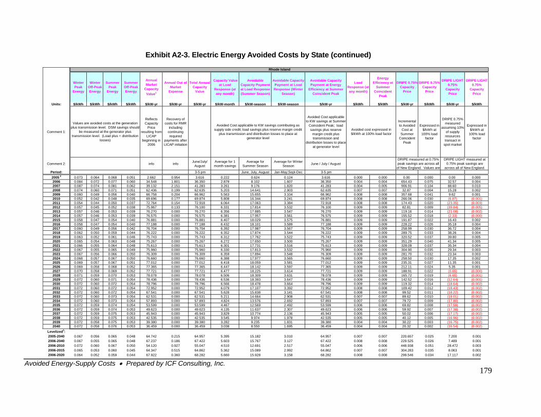
Avoided Energy-Supply Costs • Prepared by ICF Consulting, Inc.
179
Exhibit A2-3. Electric Energy Avoided Costs by State (continued)
Winter Peak
Energy
Winter Off-Peak Energy
Summer Peak
Energy
Summer Off-Peak Energy
Annual Market
Capacity Value1
Annual Out of Market
Expense
Total Annual Capacity
Value
Capacity Value at Load
Response (at any month)
Avoidable Capacity Payment at Load Response (Summer Season)
Avoidable Capacity Payment at Load Response (Winter
Season)
Avoidable Capacity Payment at Energy
Efficiency at Summer Coincident Peak
Load Response (at any month)
Energy Efficiency at
Summer Coincident
Peak
DRIPE 0.75% Capacity
Price
DRIPE 0.75% Capacity
Price
DRIPE LIGHT 0.75%
Capacity Price
DRIPE LIGHT 0.75%
Capacity Price
Units: $/kWh $/kWh $/kWh $/kWh $/kW-yr $/kW-yr $/kW-yr $/kW-month $/kW-season $/kW-season $/kW-yr $/kWh $/kWh $/kW-yr $/kWh $/kW-yr $/kWh
Comment 1:
Reflects Capacity
Price resulting from
LICAP beginning in
2006
Recovery of costs for RMR
including continuing required
payments after LICAP initiation
Avoided Cost applicable to KW savings at Summer
Coincident Peak; load savings plus reserve
margin credit plus transmission and
distribution losses to place at generator level
Incremental to Avoided
Cost at Summer
Coincident Peak
Expressed in $/kWh at
100% load factor
DRIPE 0.75% measured
assuming 10% of supply resources transact in
spot market
Expressed in $/kWh at
100% load factor
Comment 2: info info June/July/ August
Average for 1 month savings
Average for Summer Season
Average for Winter Season June / July / August
Period: 3-5 pm June, July, August Jan-May;Sept-Dec 3-5 pm2005 2 0.073 0.064 0.068 0.051 2.662 0.954 3.616 0.222 0.624 0.124 3.616 0.000 0.000 0.00 0.000 0.00 0.0002006 0.084 0.072 0.077 0.060 34.548 1.801 36.350 2.879 8.102 1.607 36.350 0.004 0.004 654.43 0.075 32.57 0.0042007 0.087 0.074 0.081 0.062 39.132 2.151 41.283 3.261 9.176 1.820 41.283 0.004 0.005 906.91 0.104 88.60 0.0102008 0.074 0.060 0.071 0.051 62.436 0.199 62.635 5.203 14.641 2.903 62.635 0.007 0.007 32.87 0.004 15.28 0.0022009 0.060 0.049 0.056 0.040 66.758 0.204 66.962 5.563 15.655 3.104 66.962 0.008 0.008 357.68 0.041 9.62 0.0012010 0.052 0.042 0.048 0.035 69.696 0.177 69.874 5.808 16.344 3.241 69.874 0.008 0.008 266.06 0.030 (6.87) (0.001)
(23.35) (0.003)(39.84) (0.005)(21.08) (0.002)(2.33) (0.000)16.43 0.002
(0.65) (0.000)(6.65) (0.001)(12.64) (0.001)(18.64) (0.002)(18.43) (0.002)(18.22) (0.002)(18.01) (0.002)(17.80) (0.002)(17.59) (0.002)(17.38) (0.002)(17.17) (0.002)(16.96) (0.002)(16.75) (0.002)(16.54) (0.002)
2011 0.054 0.044 0.050 0.037 72.764 0.154 72.918 6.064 17.063 3.384 72.918 0.008 0.008 174.43 0.0202012 0.057 0.045 0.052 0.038 75.967 0.133 76.100 6.331 17.814 3.532 76.100 0.009 0.009 82.81 0.0092013 0.057 0.046 0.053 0.039 76.270 0.000 76.270 6.356 17.885 3.547 76.270 0.009 0.009 119.16 0.0142014 0.057 0.046 0.053 0.039 76.575 0.000 76.575 6.381 17.957 3.561 76.575 0.009 0.009 155.52 0.0182015 0.058 0.047 0.054 0.040 76.881 0.000 76.881 6.407 18.029 3.575 76.881 0.009 0.009 191.87 0.0222016 0.058 0.047 0.054 0.040 77.188 0.000 77.188 6.432 18.101 3.589 77.188 0.009 0.009 228.22 0.026 35.18 0.0042017 0.060 0.049 0.056 0.042 76.704 0.000 76.704 6.392 17.987 3.567 76.704 0.009 0.009 258.99 0.030 36.72 0.0042018 0.062 0.050 0.059 0.044 76.222 0.000 76.222 6.352 17.874 3.544 76.222 0.009 0.009 289.75 0.033 38.26 0.0042019 0.063 0.052 0.061 0.046 75.743 0.000 75.743 6.312 17.762 3.522 75.743 0.009 0.009 320.52 0.037 39.80 0.0052020 0.065 0.054 0.063 0.048 75.267 0.000 75.267 6.272 17.650 3.500 75.267 0.009 0.009 351.29 0.040 41.34 0.0052021 0.066 0.055 0.064 0.048 75.613 0.000 75.613 6.301 17.731 3.516 75.613 0.009 0.009 328.09 0.037 35.34 0.0042022 0.067 0.055 0.065 0.049 75.960 0.000 75.960 6.330 17.813 3.532 75.960 0.009 0.009 304.90 0.035 29.34 0.0032023 0.067 0.056 0.066 0.050 76.309 0.000 76.309 6.359 17.894 3.548 76.309 0.009 0.009 281.70 0.032 23.34 0.0032024 0.068 0.057 0.067 0.050 76.660 0.000 76.660 6.388 17.977 3.565 76.660 0.009 0.009 258.50 0.030 17.35 0.0022025 0.069 0.057 0.067 0.051 77.012 0.000 77.012 6.418 18.059 3.581 77.012 0.009 0.009 235.31 0.027 11.35 0.0012026 0.069 0.058 0.068 0.052 77.365 0.000 77.365 6.447 18.142 3.597 77.365 0.009 0.009 212.11 0.024 5.35 0.0012027 0.070 0.058 0.069 0.052 77.721 0.000 77.721 6.477 18.225 3.614 77.721 0.009 0.009 188.91 0.0222028 0.071 0.059 0.070 0.053 78.078 0.000 78.078 6.506 18.309 3.631 78.078 0.009 0.009 165.72 0.0192029 0.072 0.060 0.071 0.054 78.436 0.000 78.436 6.536 18.393 3.647 78.436 0.009 0.009 142.52 0.0162030 0.072 0.060 0.072 0.054 78.796 0.000 78.796 6.566 18.478 3.664 78.796 0.009 0.009 119.32 0.0142031 0.072 0.060 0.072 0.054 72.952 0.000 72.952 6.079 17.107 3.392 72.952 0.008 0.008 109.42 0.0122032 0.072 0.060 0.072 0.054 67.541 0.000 67.541 5.628 15.838 3.141 67.541 0.008 0.008 99.52 0.0112033 0.072 0.060 0.073 0.054 62.531 0.000 62.531 5.211 14.664 2.908 62.531 0.007 0.007 89.62 0.0102034 0.072 0.060 0.073 0.054 57.893 0.000 57.893 4.824 13.576 2.692 57.893 0.007 0.007 79.72 0.0092035 0.072 0.059 0.074 0.054 53.599 0.000 53.599 4.467 12.569 2.492 53.599 0.006 0.006 69.82 0.0082036 0.072 0.059 0.074 0.053 49.623 0.000 49.623 4.135 11.637 2.307 49.623 0.006 0.006 59.92 0.0072037 0.072 0.059 0.075 0.053 45.943 0.000 45.943 3.829 10.774 2.136 45.943 0.005 0.005 50.02 0.0062038 0.072 0.059 0.075 0.053 42.535 0.000 42.535 3.545 9.974 1.978 42.535 0.005 0.005 40.12 0.0052039 0.072 0.058 0.075 0.053 39.380 0.000 39.380 3.282 9.235 1.831 39.380 0.004 0.004 30.22 0.0032040 0.072 0.058 0.076 0.053 36.459 0.000 36.459 3.038 8.550 1.695 36.459 0.004 0.004 20.32 0.002
Levelized3: 2005-2040 0.067 0.056 0.065 0.048 64.742 0.215 64.957 5.395 15.182 3.010 64.957 0.007 0.007 220.657 0.025 7.200 0.0012006-2040 0.067 0.055 0.065 0.048 67.237 0.186 67.422 5.603 15.767 3.127 67.422 0.008 0.008 229.525 0.026 7.489 0.0012006-2010 0.072 0.060 0.067 0.050 54.120 0.927 55.047 4.510 12.691 2.517 55.047 0.006 0.006 448.938 0.051 28.472 0.0032006-2015 0.065 0.053 0.060 0.045 64.347 0.515 64.862 5.362 15.089 2.992 64.862 0.007 0.007 304.283 0.035 8.063 0.0012006-2020 0.064 0.052 0.059 0.044 67.922 0.360 68.282 5.660 15.928 3.158 68.282 0.008 0.008 299.546 0.034 17.117 0.002
Rhode Island
Values are avoided costs at the generation plus transmission level. DSM savings should
be measured at the generator plus transmission level. (Load plus + distribution
losses)
Avoided cost expressed in $/kWh at 100% load factor
DRIPE measured at 0.75% peak savings are across all
of New England. Values are
DRIPE LIGHT measured at 0.75% peak savings are
across all of New England.
Avoided Cost applicable to KW savings contributing as supply side credit; load savings plus reserve margin credit
plus transmission and distribution losses to place at generator level
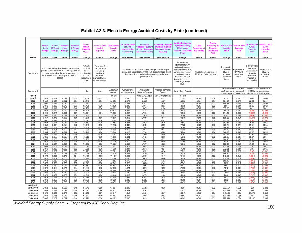
Avoided Energy-Supply Costs • Prepared by ICF Consulting, Inc.
180
Exhibit A2-3. Electric Energy Avoided Costs by State (continued)
Winter Peak
Energy
Winter Off-Peak Energy
Summer Peak
Energy
Summer Off-Peak Energy
Annual Market
Capacity Value1
Annual Out of Market
Expense
Total Annual Capacity
Value
Capacity Value at Load
Response (at any month)
Avoidable Capacity Payment at Load Response (Summer Season)
Avoidable Capacity Payment at Load Response (Winter
Season)
Avoidable Capacity Payment at Energy
Efficiency at Summer Coincident
Peak
Load Response (at any month)
Energy Efficiency at
Summer Coincident
Peak
DRIPE 0.75% Capacity
Price
DRIPE 0.75% Capacity
Price
DRIPE LIGHT 0.75%
Capacity Price
DRIPE LIGHT 0.75%
Capacity Price
Units: $/kWh $/kWh $/kWh $/kWh $/kW-yr $/kW-yr $/kW-yr $/kW-month $/kW-season $/kW-season $/kW-yr $/kWh $/kWh $/kW-yr $/kWh $/kW-yr $/kWh
Comment 1:
Reflects Capacity
Price resulting from
LICAP beginning in
2006
Recovery of costs for RMR
including continuing required
payments after LICAP initiation
Avoided Cost applicable to KW
savings at Summer Coincident Peak; load savings plus reserve
margin credit plus transmission and
distribution losses to place at generator
level
Incremental to Avoided
Cost at Summer
Coincident Peak
Expressed in $/kWh at
100% load factor
DRIPE 0.75% measured
assuming 10% of supply resources transact in
spot market
Expressed in $/kWh at
100% load factor
Comment 2: info info June/July/ August
Average for 1 month savings
Average for Summer Season
Average for Winter Season June / July / August
Period: 3-5 pm June, July, August Jan-May;Sept-Dec 3-5 pm2005 2 0.077 0.064 0.074 0.052 2.662 0.954 3.616 0.222 0.624 0.124 3.616 0.000 0.000 0.00 0.000 0.00 0.0002006 0.088 0.072 0.081 0.061 34.548 1.801 36.350 2.879 8.102 1.607 36.350 0.004 0.001 654.43 0.075 32.57 0.0042007 0.090 0.074 0.085 0.062 39.132 2.151 41.283 3.261 9.176 1.820 41.283 0.004 0.001 906.91 0.104 88.60 0.0102008 0.076 0.060 0.073 0.051 62.436 0.199 62.635 5.203 14.641 2.903 62.635 0.007 0.002 32.87 0.004 15.28 0.0022009 0.062 0.049 0.058 0.040 66.758 0.204 66.962 5.563 15.655 3.104 66.962 0.008 0.002 357.68 0.041 9.62 0.0012010 0.053 0.042 0.050 0.035 69.696 0.177 69.874 5.808 16.344 3.241 69.874 0.008 0.002 266.06 0.030 (6.87) (0.001)
(23.35) (0.003)(39.84) (0.005)(21.08) (0.002)(2.33) (0.000)16.43 0.002
(0.65) (0.000)(6.65) (0.001)(12.64) (0.001)(18.64) (0.002)(18.43) (0.002)(18.22) (0.002)(18.01) (0.002)(17.80) (0.002)(17.59) (0.002)(17.38) (0.002)(17.17) (0.002)(16.96) (0.002)(16.75) (0.002)(16.54) (0.002)
2011 0.055 0.044 0.051 0.037 72.764 0.154 72.918 6.064 17.063 3.384 72.918 0.008 0.002 174.43 0.0202012 0.056 0.046 0.052 0.038 75.967 0.133 76.100 6.331 17.814 3.532 76.100 0.009 0.002 82.81 0.0092013 0.057 0.046 0.053 0.039 76.270 0.000 76.270 6.356 17.885 3.547 76.270 0.009 0.002 119.16 0.0142014 0.057 0.047 0.053 0.039 76.575 0.000 76.575 6.381 17.957 3.561 76.575 0.009 0.002 155.52 0.0182015 0.058 0.047 0.054 0.040 76.881 0.000 76.881 6.407 18.029 3.575 76.881 0.009 0.002 191.87 0.0222016 0.058 0.048 0.055 0.040 77.188 0.000 77.188 6.432 18.101 3.589 77.188 0.009 0.002 228.22 0.026 35.18 0.0042017 0.060 0.049 0.057 0.042 76.704 0.000 76.704 6.392 17.987 3.567 76.704 0.009 0.002 258.99 0.030 36.72 0.0042018 0.062 0.051 0.059 0.044 76.222 0.000 76.222 6.352 17.874 3.544 76.222 0.009 0.002 289.75 0.033 38.26 0.0042019 0.064 0.053 0.061 0.046 75.743 0.000 75.743 6.312 17.762 3.522 75.743 0.009 0.002 320.52 0.037 39.80 0.0052020 0.065 0.055 0.064 0.048 75.267 0.000 75.267 6.272 17.650 3.500 75.267 0.009 0.002 351.29 0.040 41.34 0.0052021 0.066 0.055 0.065 0.049 75.613 0.000 75.613 6.301 17.731 3.516 75.613 0.009 0.002 328.09 0.037 35.34 0.0042022 0.067 0.056 0.066 0.049 75.960 0.000 75.960 6.330 17.813 3.532 75.960 0.009 0.002 304.90 0.035 29.34 0.0032023 0.068 0.056 0.066 0.050 76.309 0.000 76.309 6.359 17.894 3.548 76.309 0.009 0.002 281.70 0.032 23.34 0.0032024 0.068 0.057 0.067 0.051 76.660 0.000 76.660 6.388 17.977 3.565 76.660 0.009 0.002 258.50 0.030 17.35 0.0022025 0.069 0.058 0.068 0.051 77.012 0.000 77.012 6.418 18.059 3.581 77.012 0.009 0.002 235.31 0.027 11.35 0.0012026 0.070 0.058 0.069 0.052 77.365 0.000 77.365 6.447 18.142 3.597 77.365 0.009 0.002 212.11 0.024 5.35 0.0012027 0.071 0.059 0.070 0.053 77.721 0.000 77.721 6.477 18.225 3.614 77.721 0.009 0.002 188.91 0.0222028 0.071 0.059 0.071 0.054 78.078 0.000 78.078 6.506 18.309 3.631 78.078 0.009 0.002 165.72 0.0192029 0.072 0.060 0.072 0.054 78.436 0.000 78.436 6.536 18.393 3.647 78.436 0.009 0.002 142.52 0.0162030 0.073 0.061 0.073 0.055 78.796 0.000 78.796 6.566 18.478 3.664 78.796 0.009 0.002 119.32 0.0142031 0.073 0.060 0.073 0.055 72.952 0.000 72.952 6.079 17.107 3.392 72.952 0.008 0.002 109.42 0.0122032 0.073 0.060 0.073 0.055 67.541 0.000 67.541 5.628 15.838 3.141 67.541 0.008 0.002 99.52 0.0112033 0.073 0.060 0.074 0.054 62.531 0.000 62.531 5.211 14.664 2.908 62.531 0.007 0.002 89.62 0.0102034 0.073 0.060 0.074 0.054 57.893 0.000 57.893 4.824 13.576 2.692 57.893 0.007 0.002 79.72 0.0092035 0.073 0.060 0.075 0.054 53.599 0.000 53.599 4.467 12.569 2.492 53.599 0.006 0.001 69.82 0.0082036 0.073 0.060 0.075 0.054 49.623 0.000 49.623 4.135 11.637 2.307 49.623 0.006 0.001 59.92 0.0072037 0.073 0.059 0.075 0.054 45.943 0.000 45.943 3.829 10.774 2.136 45.943 0.005 0.001 50.02 0.0062038 0.073 0.059 0.076 0.053 42.535 0.000 42.535 3.545 9.974 1.978 42.535 0.005 0.001 40.12 0.0052039 0.073 0.059 0.076 0.053 39.380 0.000 39.380 3.282 9.235 1.831 39.380 0.004 0.001 30.22 0.0032040 0.073 0.059 0.076 0.053 36.459 0.000 36.459 3.038 8.550 1.695 36.459 0.004 0.001 20.32 0.002
Levelized3: 2005-2040 0.068 0.056 0.066 0.049 64.742 0.215 64.957 5.395 15.182 3.010 64.957 0.007 0.002 220.657 0.025 7.200 0.0012006-2040 0.068 0.056 0.066 0.048 67.237 0.186 67.422 5.603 15.767 3.127 67.422 0.008 0.002 229.525 0.026 7.489 0.0012006-2010 0.074 0.060 0.070 0.050 54.120 0.927 55.047 4.510 12.691 2.517 55.047 0.006 0.001 448.938 0.051 28.472 0.0032006-2015 0.066 0.053 0.062 0.045 64.347 0.515 64.862 5.362 15.089 2.992 64.862 0.007 0.002 304.283 0.035 8.063 0.0012006-2020 0.065 0.053 0.061 0.044 67.922 0.360 68.282 5.660 15.928 3.158 68.282 0.008 0.002 299.546 0.034 17.117 0.002
Vermont
Avoided cost expressed in $/kWh at 100% load factor
Values are avoided costs at the generation plus transmission level. DSM savings should
be measured at the generator plus transmission level. (Load plus + distribution
losses)
Avoided Cost applicable to KW savings contributing as supply side credit; load savings plus reserve margin credit
plus transmission and distribution losses to place at generator level
DRIPE measured at 0.75% peak savings are across all
of New England. Values are
DRIPE LIGHT measured at 0.75% peak savings are
across all of New England.
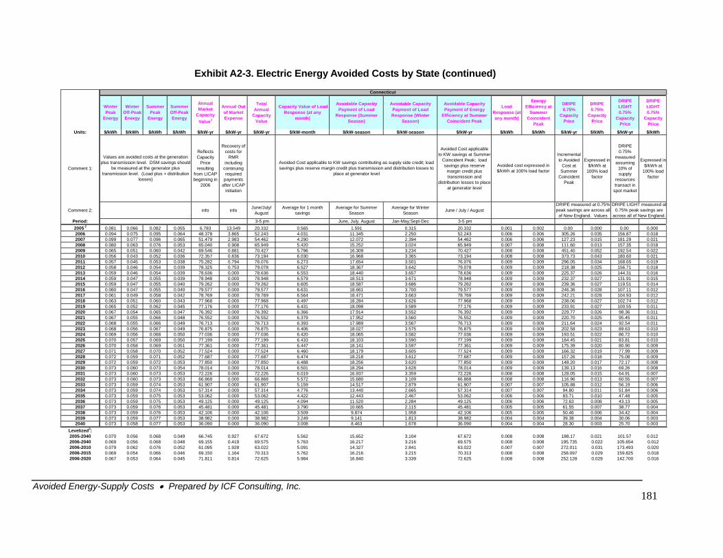
Avoided Energy-Supply Costs • Prepared by ICF Consulting, Inc.
181
Exhibit A2-3. Electric Energy Avoided Costs by State (continued)
Winter Peak
Energy
Winter Off-Peak Energy
Summer Peak
Energy
Summer Off-Peak Energy
Annual Market
Capacity Value1
Annual Out of Market Expense
Total Annual
Capacity Value
Capacity Value of Load Response (at any
month)
Avoidable Capacity Payment of Load
Response (Summer Season)
Avoidable Capacity Payment of Load Response (Winter
Season)
Avoidable Capacity Payment of Energy
Efficiency at Summer Coincident Peak
Load Response (at any month)
Energy Efficiency at
Summer Coincident
Peak
DRIPE 0.75%
Capacity Price
DRIPE 0.75%
Capacity Price
DRIPE LIGHT 0.75%
Capacity Price
DRIPE LIGHT 0.75%
Capacity Price
Units: $/kWh $/kWh $/kWh $/kWh $/kW-yr $/kW-yr $/kW-yr $/kW-month $/kW-season $/kW-season $/kW-yr $/kWh $/kWh $/kW-yr $/kWh $/kW-yr $/kWh
Comment 1:
Reflects Capacity
Price resulting
from LICAP beginning in
2006
Recovery of costs for
RMR including
continuing required
payments after LICAP
initiation
Avoided Cost applicable to KW savings at Summer
Coincident Peak; load savings plus reserve
margin credit plus transmission and
distribution losses to place at generator level
Incremental to Avoided
Cost at Summer
Coincident Peak
Expressed in $/kWh at
100% load factor
DRIPE 0.75%
measured assuming
10% of supply
resources transact in
spot market
Expressed in $/kWh at
100% load factor
Comment 2: info info June/July/ August
Average for 1 month savings
Average for Summer Season
Average for Winter Season June / July / August
Period: 3-5 pm June, July, August Jan-May;Sept-Dec 3-5 pm2005 2 0.081 0.066 0.082 0.055 6.783 13.549 20.332 0.565 1.591 0.315 20.332 0.001 0.002 0.00 0.000 0.00 0.0002006 0.094 0.075 0.095 0.064 48.378 3.865 52.243 4.031 11.345 2.250 52.243 0.006 0.006 305.26 0.035 156.87 0.0182007 0.099 0.077 0.096 0.065 51.479 2.983 54.462 4.290 12.072 2.394 54.462 0.006 0.006 127.23 0.015 181.29 0.0212008 0.080 0.063 0.076 0.053 65.040 0.908 65.949 5.420 15.252 3.024 65.949 0.007 0.008 111.60 0.013 157.35 0.0182009 0.065 0.051 0.060 0.042 69.546 0.881 70.427 5.796 16.309 3.234 70.427 0.008 0.008 451.40 0.052 192.54 0.0222010 0.056 0.043 0.052 0.036 72.357 0.836 73.194 6.030 16.968 3.365 73.194 0.008 0.008 373.73 0.043 180.60 0.0212011 0.057 0.045 0.053 0.038 75.282 0.794 76.076 6.273 17.654 3.501 76.076 0.009 0.009 296.05 0.034 168.65 0.0192012 0.058 0.046 0.054 0.039 78.325 0.753 79.078 6.527 18.367 3.642 79.078 0.009 0.009 218.38 0.025 156.71 0.0182013 0.059 0.046 0.054 0.039 78.636 0.000 78.636 6.553 18.440 3.657 78.636 0.009 0.009 225.37 0.026 144.31 0.0162014 0.059 0.047 0.055 0.039 78.948 0.000 78.948 6.579 18.513 3.671 78.948 0.009 0.009 232.37 0.027 131.91 0.0152015 0.059 0.047 0.055 0.040 79.262 0.000 79.262 6.605 18.587 3.686 79.262 0.009 0.009 239.36 0.027 119.51 0.0142016 0.060 0.047 0.055 0.040 79.577 0.000 79.577 6.631 18.661 3.700 79.577 0.009 0.009 246.36 0.028 107.11 0.0122017 0.061 0.049 0.058 0.042 78.769 0.000 78.769 6.564 18.471 3.663 78.769 0.009 0.009 242.21 0.028 104.93 0.0122018 0.063 0.051 0.060 0.043 77.968 0.000 77.968 6.497 18.284 3.626 77.968 0.009 0.009 238.06 0.027 102.74 0.0122019 0.065 0.052 0.062 0.045 77.176 0.000 77.176 6.431 18.098 3.589 77.176 0.009 0.009 233.91 0.027 100.55 0.0112020 0.067 0.054 0.065 0.047 76.392 0.000 76.392 6.366 17.914 3.552 76.392 0.009 0.009 229.77 0.026 98.36 0.0112021 0.067 0.055 0.066 0.048 76.552 0.000 76.552 6.379 17.952 3.560 76.552 0.009 0.009 220.70 0.025 95.45 0.0112022 0.068 0.055 0.066 0.049 76.713 0.000 76.713 6.393 17.989 3.567 76.713 0.009 0.009 211.64 0.024 92.54 0.0112023 0.068 0.056 0.067 0.049 76.875 0.000 76.875 6.406 18.027 3.575 76.875 0.009 0.009 202.58 0.023 89.63 0.0102024 0.069 0.056 0.068 0.050 77.036 0.000 77.036 6.420 18.065 3.582 77.036 0.009 0.009 193.51 0.022 86.72 0.0102025 0.070 0.057 0.069 0.050 77.199 0.000 77.199 6.433 18.103 3.590 77.199 0.009 0.009 184.45 0.021 83.81 0.0102026 0.070 0.058 0.069 0.051 77.361 0.000 77.361 6.447 18.141 3.597 77.361 0.009 0.009 175.39 0.020 80.90 0.0092027 0.071 0.058 0.070 0.052 77.524 0.000 77.524 6.460 18.179 3.605 77.524 0.009 0.009 166.32 0.019 77.99 0.0092028 0.072 0.059 0.071 0.052 77.687 0.000 77.687 6.474 18.218 3.612 77.687 0.009 0.009 157.26 0.018 75.08 0.0092029 0.072 0.059 0.072 0.053 77.850 0.000 77.850 6.488 18.256 3.620 77.850 0.009 0.009 148.20 0.017 72.17 0.0082030 0.073 0.060 0.073 0.054 78.014 0.000 78.014 6.501 18.294 3.628 78.014 0.009 0.009 139.13 0.016 69.26 0.0082031 0.073 0.060 0.073 0.053 72.226 0.000 72.226 6.019 16.937 3.359 72.226 0.008 0.008 128.05 0.015 64.91 0.0072032 0.073 0.060 0.073 0.053 66.868 0.000 66.868 5.572 15.680 3.109 66.868 0.008 0.008 116.96 0.013 60.55 0.0072033 0.073 0.059 0.074 0.053 61.907 0.000 61.907 5.159 14.517 2.879 61.907 0.007 0.007 105.88 0.012 56.19 0.0062034 0.073 0.059 0.074 0.053 57.314 0.000 57.314 4.776 13.440 2.665 57.314 0.007 0.007 94.80 0.011 51.84 0.0062035 0.073 0.059 0.075 0.053 53.062 0.000 53.062 4.422 12.443 2.467 53.062 0.006 0.006 83.71 0.010 47.48 0.0052036 0.073 0.059 0.075 0.053 49.125 0.000 49.125 4.094 11.520 2.284 49.125 0.006 0.006 72.63 0.008 43.13 0.0052037 0.073 0.059 0.076 0.053 45.481 0.000 45.481 3.790 10.665 2.115 45.481 0.005 0.005 61.55 0.007 38.77 0.0042038 0.073 0.059 0.076 0.053 42.106 0.000 42.106 3.509 9.874 1.958 42.106 0.005 0.005 50.46 0.006 34.42 0.0042039 0.073 0.059 0.077 0.053 38.982 0.000 38.982 3.249 9.141 1.813 38.982 0.004 0.004 39.38 0.004 30.06 0.0032040 0.073 0.058 0.077 0.053 36.090 0.000 36.090 3.008 8.463 1.678 36.090 0.004 0.004 28.30 0.003 25.70 0.003
Levelized3: 2005-2040 0.070 0.056 0.068 0.049 66.745 0.927 67.672 5.562 15.652 3.104 67.672 0.008 0.008 188.17 0.021 101.57 0.0122006-2040 0.069 0.056 0.068 0.048 69.155 0.419 69.575 5.763 16.217 3.216 69.575 0.008 0.008 195.735 0.022 105.654 0.0122006-2010 0.079 0.062 0.076 0.052 61.095 1.928 63.022 5.091 14.327 2.841 63.022 0.007 0.007 272.011 0.031 173.493 0.0202006-2015 0.069 0.054 0.066 0.046 69.150 1.164 70.313 5.762 16.216 3.215 70.313 0.008 0.008 258.097 0.029 159.825 0.0182006-2020 0.067 0.053 0.064 0.045 71.811 0.814 72.625 5.984 16.840 3.339 72.625 0.008 0.008 252.128 0.029 142.700 0.016
Values are avoided costs at the generation plus transmission level. DSM savings should
be measured at the generator plus transmission level. (Load plus + distribution
losses)
Avoided cost expressed in $/kWh at 100% load factor
Avoided Cost applicable to KW savings contributing as supply side credit; load savings plus reserve margin credit plus transmission and distribution losses to
place at generator level
DRIPE measured at 0.75% peak savings are across all
of New England. Values
DRIPE LIGHT measured at 0.75% peak savings are
across all of New England.
Connecticut
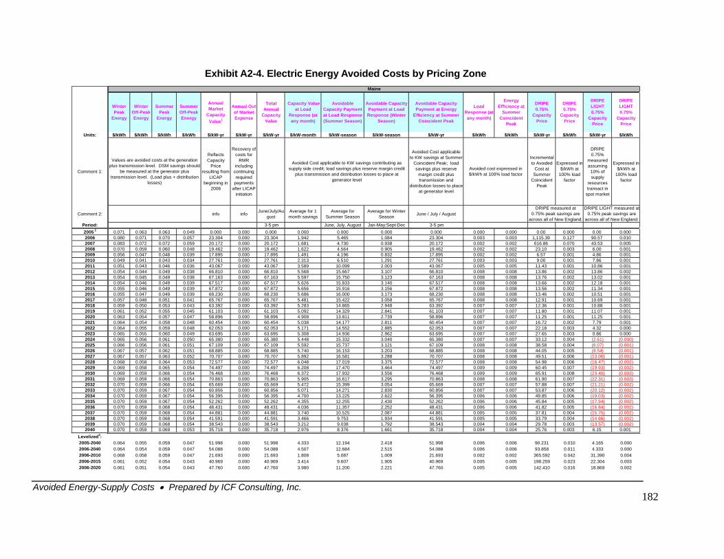
Avoided Energy-Supply Costs • Prepared by ICF Consulting, Inc.
182
Exhibit A2-4. Electric Energy Avoided Costs by Pricing Zone
Winter Peak
Energy
Winter Off-Peak Energy
Summer Peak
Energy
Summer Off-Peak Energy
Annual Market
Capacity Value1
Annual Out of Market Expense
Total Annual
Capacity Value
Capacity Value at Load
Response (at any month)
Avoidable Capacity Payment at Load Response (Summer Season)
Avoidable Capacity Payment at Load Response (Winter
Season)
Avoidable Capacity Payment at Energy
Efficiency at Summer Coincident Peak
Load Response (at any month)
Energy Efficiency at
Summer Coincident
Peak
DRIPE 0.75%
Capacity Price
DRIPE 0.75%
Capacity Price
DRIPE LIGHT 0.75%
Capacity Price
DRIPE LIGHT 0.75%
Capacity Price
Units: $/kWh $/kWh $/kWh $/kWh $/kW-yr $/kW-yr $/kW-yr $/kW-month $/kW-season $/kW-season $/kW-yr $/kWh $/kWh $/kW-yr $/kWh $/kW-yr $/kWh
Comment 1:
Reflects Capacity
Price resulting from
LICAP beginning in
2006
Recovery of costs for
RMR including
continuing required
payments after LICAP
initiation
Avoided Cost applicable to KW savings at Summer
Coincident Peak; load savings plus reserve
margin credit plus transmission and
distribution losses to place at generator level
Incremental to Avoided
Cost at Summer
Coincident Peak
Expressed in $/kWh at
100% load factor
DRIPE 0.75%
measured assuming
10% of supply
resources transact in
spot market
Expressed in $/kWh at
100% load factor
Comment 2: info info June/July/August
Average for 1 month savings
Average for Summer Season
Average for Winter Season June / July / August
Period: 3-5 pm June, July, August Jan-May;Sept-Dec 3-5 pm2005 2 0.071 0.063 0.063 0.049 0.000 0.000 0.000 0.000 0.000 0.000 0.000 0.000 0.000 0.00 0.000 0.00 0.0002006 0.080 0.071 0.070 0.057 23.304 0.000 23.304 1.942 5.465 1.084 23.304 0.003 0.003 1,115.39 0.127 90.57 0.0102007 0.083 0.072 0.072 0.059 20.172 0.000 20.172 1.681 4.730 0.938 20.172 0.002 0.002 616.86 0.070 43.53 0.0052008 0.070 0.059 0.060 0.048 19.462 0.000 19.462 1.622 4.564 0.905 19.462 0.002 0.002 23.10 0.003 6.00 0.0012009 0.056 0.047 0.048 0.039 17.895 0.000 17.895 1.491 4.196 0.832 17.895 0.002 0.002 6.57 0.001 4.86 0.0012010 0.049 0.041 0.043 0.034 27.761 0.000 27.761 2.313 6.510 1.291 27.761 0.003 0.003 9.00 0.001 7.86 0.0012011 0.051 0.043 0.046 0.036 43.067 0.000 43.067 3.589 10.099 2.003 43.067 0.005 0.005 11.43 0.001 10.86 0.0012012 0.054 0.044 0.049 0.038 66.810 0.000 66.810 5.568 15.667 3.107 66.810 0.008 0.008 13.86 0.002 13.86 0.0022013 0.054 0.045 0.049 0.038 67.163 0.000 67.163 5.597 15.750 3.123 67.163 0.008 0.008 13.76 0.002 13.02 0.0012014 0.054 0.046 0.049 0.039 67.517 0.000 67.517 5.626 15.833 3.140 67.517 0.008 0.008 13.66 0.002 12.18 0.0012015 0.055 0.046 0.049 0.039 67.872 0.000 67.872 5.656 15.916 3.156 67.872 0.008 0.008 13.56 0.002 11.34 0.0012016 0.055 0.047 0.049 0.039 68.230 0.000 68.230 5.686 16.000 3.173 68.230 0.008 0.008 13.46 0.002 10.51 0.0012017 0.057 0.048 0.051 0.041 65.767 0.000 65.767 5.481 15.422 3.058 65.767 0.008 0.008 12.91 0.001 10.69 0.0012018 0.059 0.050 0.053 0.043 63.392 0.000 63.392 5.283 14.865 2.948 63.392 0.007 0.007 12.36 0.001 10.88 0.0012019 0.061 0.052 0.055 0.045 61.103 0.000 61.103 5.092 14.329 2.841 61.103 0.007 0.007 11.80 0.001 11.07 0.0012020 0.063 0.054 0.057 0.047 58.896 0.000 58.896 4.908 13.811 2.739 58.896 0.007 0.007 11.25 0.001 11.25 0.0012021 0.064 0.054 0.058 0.048 60.454 0.000 60.454 5.038 14.177 2.811 60.454 0.007 0.007 16.72 0.002 7.79 0.0012022 0.064 0.055 0.059 0.048 62.053 0.000 62.053 5.171 14.552 2.885 62.053 0.007 0.007 22.18 0.003 4.32 0.0002023 0.065 0.055 0.060 0.049 63.695 0.000 63.695 5.308 14.936 2.962 63.695 0.007 0.007 27.65 0.003 0.86 0.0002024 0.065 0.056 0.061 0.050 65.380 0.000 65.380 5.448 15.332 3.040 65.380 0.007 0.007 33.12 0.004 (2.61) (0.000)
(6.07) (0.001)(9.54) (0.001)
(13.00) (0.001)(16.47) (0.002)(19.93) (0.002)(23.40) (0.003)(22.31) (0.003)(21.21) (0.002)(20.12) (0.002)(19.03) (0.002)(17.94) (0.002)(16.84) (0.002)(15.75) (0.002)(14.66) (0.002)(13.57) (0.002)6.15 0.001
2025 0.066 0.056 0.061 0.051 67.109 0.000 67.109 5.592 15.737 3.121 67.109 0.008 0.008 38.58 0.0042026 0.067 0.057 0.062 0.051 68.885 0.000 68.885 5.740 16.153 3.203 68.885 0.008 0.008 44.05 0.0052027 0.067 0.057 0.063 0.052 70.707 0.000 70.707 5.892 16.581 3.288 70.707 0.008 0.008 49.51 0.0062028 0.068 0.058 0.064 0.053 72.577 0.000 72.577 6.048 17.019 3.375 72.577 0.008 0.008 54.98 0.0062029 0.069 0.058 0.065 0.054 74.497 0.000 74.497 6.208 17.470 3.464 74.497 0.009 0.009 60.45 0.0072030 0.069 0.059 0.066 0.054 76.468 0.000 76.468 6.372 17.932 3.556 76.468 0.009 0.009 65.91 0.0082031 0.069 0.059 0.066 0.054 70.863 0.000 70.863 5.905 16.617 3.295 70.863 0.008 0.008 61.90 0.0072032 0.070 0.059 0.066 0.054 65.669 0.000 65.669 5.472 15.399 3.054 65.669 0.007 0.007 57.88 0.0072033 0.070 0.059 0.067 0.054 60.856 0.000 60.856 5.071 14.271 2.830 60.856 0.007 0.007 53.87 0.0062034 0.070 0.059 0.067 0.054 56.395 0.000 56.395 4.700 13.225 2.622 56.395 0.006 0.006 49.85 0.0062035 0.070 0.059 0.067 0.054 52.262 0.000 52.262 4.355 12.255 2.430 52.262 0.006 0.006 45.84 0.0052036 0.070 0.059 0.068 0.054 48.431 0.000 48.431 4.036 11.357 2.252 48.431 0.006 0.006 41.82 0.0052037 0.070 0.059 0.068 0.054 44.881 0.000 44.881 3.740 10.525 2.087 44.881 0.005 0.005 37.81 0.0042038 0.070 0.059 0.068 0.054 41.591 0.000 41.591 3.466 9.753 1.934 41.591 0.005 0.005 33.79 0.0042039 0.070 0.059 0.068 0.054 38.543 0.000 38.543 3.212 9.038 1.792 38.543 0.004 0.004 29.78 0.0032040 0.070 0.059 0.069 0.053 35.718 0.000 35.718 2.976 8.376 1.661 35.718 0.004 0.004 25.76 0.003
Levelized3: 2005-2040 0.064 0.055 0.059 0.047 51.998 0.000 51.998 4.333 12.194 2.418 51.998 0.006 0.006 90.231 0.010 4.165 0.0002006-2040 0.064 0.054 0.059 0.047 54.088 0.000 54.088 4.507 12.684 2.515 54.088 0.006 0.006 93.858 0.011 4.333 0.0002006-2010 0.068 0.058 0.059 0.047 21.693 0.000 21.693 1.808 5.087 1.009 21.693 0.002 0.002 365.592 0.042 31.390 0.0042006-2015 0.061 0.052 0.054 0.043 40.969 0.000 40.969 3.414 9.607 1.905 40.969 0.005 0.005 198.259 0.023 22.304 0.0032006-2020 0.061 0.051 0.054 0.043 47.760 0.000 47.760 3.980 11.200 2.221 47.760 0.005 0.005 142.410 0.016 18.869 0.002
Avoided Cost applicable to KW savings contributing as supply side credit; load savings plus reserve margin credit
plus transmission and distribution losses to place at generator level
Values are avoided costs at the generation plus transmission level. DSM savings should
be measured at the generator plus transmission level. (Load plus + distribution
losses)
Avoided cost expressed in $/kWh at 100% load factor
Maine
DRIPE measured at 0.75% peak savings are
across all of New England.
DRIPE LIGHT measured at 0.75% peak savings are
across all of New England.
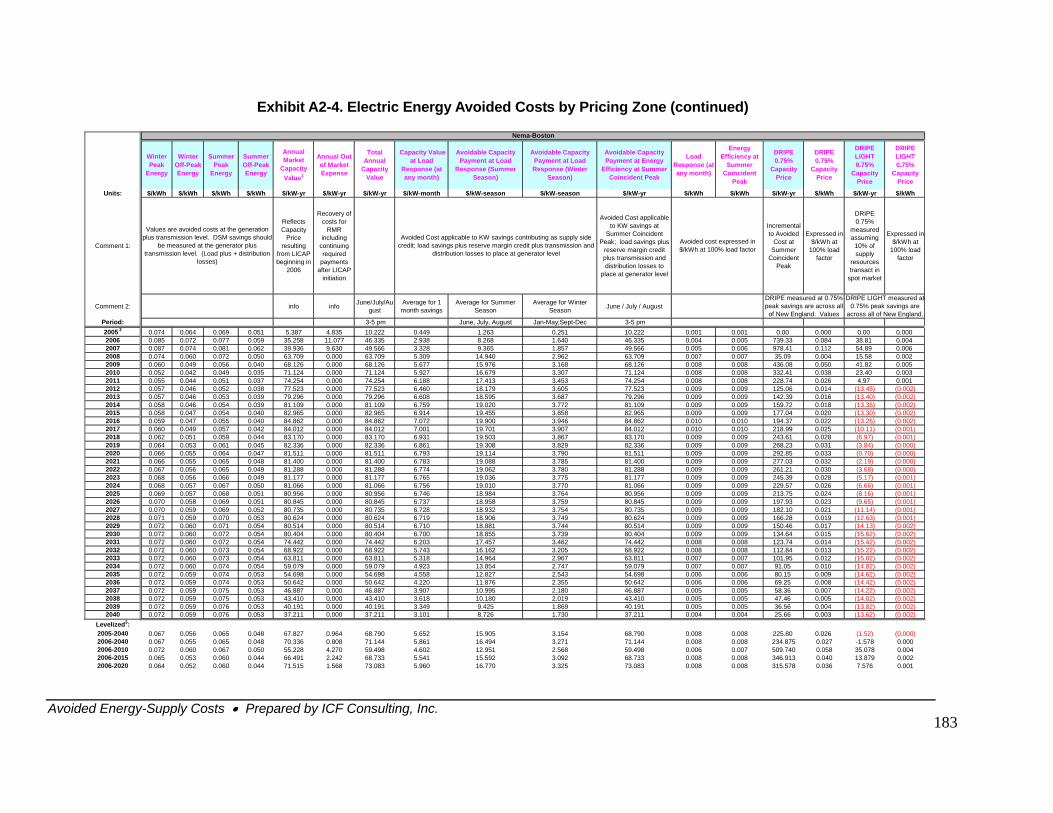
Avoided Energy-Supply Costs • Prepared by ICF Consulting, Inc.
183
Exhibit A2-4. Electric Energy Avoided Costs by Pricing Zone (continued)
Winter Peak
Energy
Winter Off-Peak Energy
Summer Peak
Energy
Summer Off-Peak Energy
Annual Market
Capacity Value1
Annual Out of Market Expense
Total Annual
Capacity Value
Capacity Value at Load
Response (at any month)
Avoidable Capacity Payment at Load
Response (Summer Season)
Avoidable Capacity Payment at Load Response (Winter
Season)
Avoidable Capacity Payment at Energy
Efficiency at Summer Coincident Peak
Load Response (at any month)
Energy Efficiency at
Summer Coincident
Peak
DRIPE 0.75%
Capacity Price
DRIPE 0.75%
Capacity Price
DRIPE LIGHT 0.75%
Capacity Price
DRIPE LIGHT 0.75%
Capacity Price
Units: $/kWh $/kWh $/kWh $/kWh $/kW-yr $/kW-yr $/kW-yr $/kW-month $/kW-season $/kW-season $/kW-yr $/kWh $/kWh $/kW-yr $/kWh $/kW-yr $/kWh
Comment 1:
Reflects Capacity
Price resulting
from LICAP beginning in
2006
Recovery of costs for
RMR including
continuing required
payments after LICAP
initiation
Avoided Cost applicable to KW savings at
Summer Coincident Peak; load savings plus
reserve margin credit plus transmission and distribution losses to
place at generator level
Incremental to Avoided
Cost at Summer
Coincident Peak
Expressed in $/kWh at
100% load factor
DRIPE 0.75%
measured assuming
10% of supply
resources transact in
spot market
Expressed in $/kWh at
100% load factor
Comment 2: info info June/July/August
Average for 1 month savings
Average for Summer Season
Average for Winter Season June / July / August
Period: 3-5 pm June, July, August Jan-May;Sept-Dec 3-5 pm2005 2 0.074 0.064 0.069 0.051 5.387 4.835 10.222 0.449 1.263 0.251 10.222 0.001 0.001 0.00 0.000 0.00 0.0002006 0.085 0.072 0.077 0.059 35.258 11.077 46.335 2.938 8.268 1.640 46.335 0.004 0.005 739.33 0.084 38.81 0.0042007 0.087 0.074 0.081 0.062 39.936 9.630 49.566 3.328 9.365 1.857 49.566 0.005 0.006 978.41 0.112 54.89 0.0062008 0.074 0.060 0.072 0.050 63.709 0.000 63.709 5.309 14.940 2.962 63.709 0.007 0.007 35.09 0.004 15.58 0.0022009 0.060 0.049 0.056 0.040 68.126 0.000 68.126 5.677 15.976 3.168 68.126 0.008 0.008 436.08 0.050 41.82 0.0052010 0.052 0.042 0.049 0.035 71.124 0.000 71.124 5.927 16.679 3.307 71.124 0.008 0.008 332.41 0.038 23.40 0.0032011 0.055 0.044 0.051 0.037 74.254 0.000 74.254 6.188 17.413 3.453 74.254 0.008 0.008 228.74 0.026 4.97 0.0012012 0.057 0.046 0.052 0.038 77.523 0.000 77.523 6.460 18.179 3.605 77.523 0.009 0.009 125.06 0.014 (13.45) (0.002)2013 0.057 0.046 0.053 0.039 79.296 0.000 79.296 6.608 18.595 3.687 79.296 0.009 0.009 142.39 0.016 (13.40) (0.002)2014 0.058 0.046 0.054 0.039 81.109 0.000 81.109 6.759 19.020 3.772 81.109 0.009 0.009 159.72 0.018 (13.35) (0.002)2015 0.058 0.047 0.054 0.040 82.965 0.000 82.965 6.914 19.455 3.858 82.965 0.009 0.009 177.04 0.020 (13.30) (0.002)2016 0.059 0.047 0.055 0.040 84.862 0.000 84.862 7.072 19.900 3.946 84.862 0.010 0.010 194.37 0.022 (13.25) (0.002)2017 0.060 0.049 0.057 0.042 84.012 0.000 84.012 7.001 19.701 3.907 84.012 0.010 0.010 218.99 0.025 (10.11) (0.001)2018 0.062 0.051 0.059 0.044 83.170 0.000 83.170 6.931 19.503 3.867 83.170 0.009 0.009 243.61 0.028 (6.97) (0.001)2019 0.064 0.053 0.061 0.045 82.336 0.000 82.336 6.861 19.308 3.829 82.336 0.009 0.009 268.23 0.031 (3.84) (0.000)2020 0.066 0.055 0.064 0.047 81.511 0.000 81.511 6.793 19.114 3.790 81.511 0.009 0.009 292.85 0.033 (0.70) (0.000)2021 0.066 0.055 0.065 0.048 81.400 0.000 81.400 6.783 19.088 3.785 81.400 0.009 0.009 277.03 0.032 (2.19) (0.000)2022 0.067 0.056 0.065 0.049 81.288 0.000 81.288 6.774 19.062 3.780 81.288 0.009 0.009 261.21 0.030 (3.68) (0.000)2023 0.068 0.056 0.066 0.049 81.177 0.000 81.177 6.765 19.036 3.775 81.177 0.009 0.009 245.39 0.028 (5.17) (0.001)2024 0.068 0.057 0.067 0.050 81.066 0.000 81.066 6.756 19.010 3.770 81.066 0.009 0.009 229.57 0.026 (6.66) (0.001)2025 0.069 0.057 0.068 0.051 80.956 0.000 80.956 6.746 18.984 3.764 80.956 0.009 0.009 213.75 0.024 (8.16) (0.001)2026 0.070 0.058 0.069 0.051 80.845 0.000 80.845 6.737 18.958 3.759 80.845 0.009 0.009 197.93 0.023 (9.65) (0.001)2027 0.070 0.059 0.069 0.052 80.735 0.000 80.735 6.728 18.932 3.754 80.735 0.009 0.009 182.10 0.021 (11.14) (0.001)2028 0.071 0.059 0.070 0.053 80.624 0.000 80.624 6.719 18.906 3.749 80.624 0.009 0.009 166.28 0.019 (12.63) (0.001)2029 0.072 0.060 0.071 0.054 80.514 0.000 80.514 6.710 18.881 3.744 80.514 0.009 0.009 150.46 0.017 (14.13) (0.002)2030 0.072 0.060 0.072 0.054 80.404 0.000 80.404 6.700 18.855 3.739 80.404 0.009 0.009 134.64 0.015 (15.62) (0.002)2031 0.072 0.060 0.072 0.054 74.442 0.000 74.442 6.203 17.457 3.462 74.442 0.008 0.008 123.74 0.014 (15.42) (0.002)2032 0.072 0.060 0.073 0.054 68.922 0.000 68.922 5.743 16.162 3.205 68.922 0.008 0.008 112.84 0.013 (15.22) (0.002)2033 0.072 0.060 0.073 0.054 63.811 0.000 63.811 5.318 14.964 2.967 63.811 0.007 0.007 101.95 0.012 (15.02) (0.002)2034 0.072 0.060 0.074 0.054 59.079 0.000 59.079 4.923 13.854 2.747 59.079 0.007 0.007 91.05 0.010 (14.82) (0.002)2035 0.072 0.059 0.074 0.053 54.698 0.000 54.698 4.558 12.827 2.543 54.698 0.006 0.006 80.15 0.009 (14.62) (0.002)2036 0.072 0.059 0.074 0.053 50.642 0.000 50.642 4.220 11.876 2.355 50.642 0.006 0.006 69.25 0.008 (14.42) (0.002)2037 0.072 0.059 0.075 0.053 46.887 0.000 46.887 3.907 10.995 2.180 46.887 0.005 0.005 58.36 0.007 (14.22) (0.002)2038 0.072 0.059 0.075 0.053 43.410 0.000 43.410 3.618 10.180 2.019 43.410 0.005 0.005 47.46 0.005 (14.02) (0.002)2039 0.072 0.059 0.076 0.053 40.191 0.000 40.191 3.349 9.425 1.869 40.191 0.005 0.005 36.56 0.004 (13.82) (0.002)2040 0.072 0.059 0.076 0.053 37.211 0.000 37.211 3.101 8.726 1.730 37.211 0.004 0.004 25.66 0.003 (13.62) (0.002)
Levelized3: 2005-2040 0.067 0.056 0.065 0.048 67.827 0.964 68.790 5.652 15.905 3.154 68.790 0.008 0.008 225.80 0.026 (1.52) (0.000)2006-2040 0.067 0.055 0.065 0.048 70.336 0.808 71.144 5.861 16.494 3.271 71.144 0.008 0.008 234.875 0.027 -1.578 0.0002006-2010 0.072 0.060 0.067 0.050 55.228 4.270 59.498 4.602 12.951 2.568 59.498 0.006 0.007 509.740 0.058 35.078 0.0042006-2015 0.065 0.053 0.060 0.044 66.491 2.242 68.733 5.541 15.592 3.092 68.733 0.008 0.008 346.913 0.040 13.879 0.0022006-2020 0.064 0.052 0.060 0.044 71.515 1.568 73.083 5.960 16.770 3.325 73.083 0.008 0.008 315.578 0.036 7.576 0.001
Nema-Boston
DRIPE measured at 0.75% peak savings are across all
of New England. Values
DRIPE LIGHT measured at 0.75% peak savings are
across all of New England.
Values are avoided costs at the generation plus transmission level. DSM savings should
be measured at the generator plus transmission level. (Load plus + distribution
losses)
Avoided cost expressed in $/kWh at 100% load factor
Avoided Cost applicable to KW savings contributing as supply side credit; load savings plus reserve margin credit plus transmission and
distribution losses to place at generator level
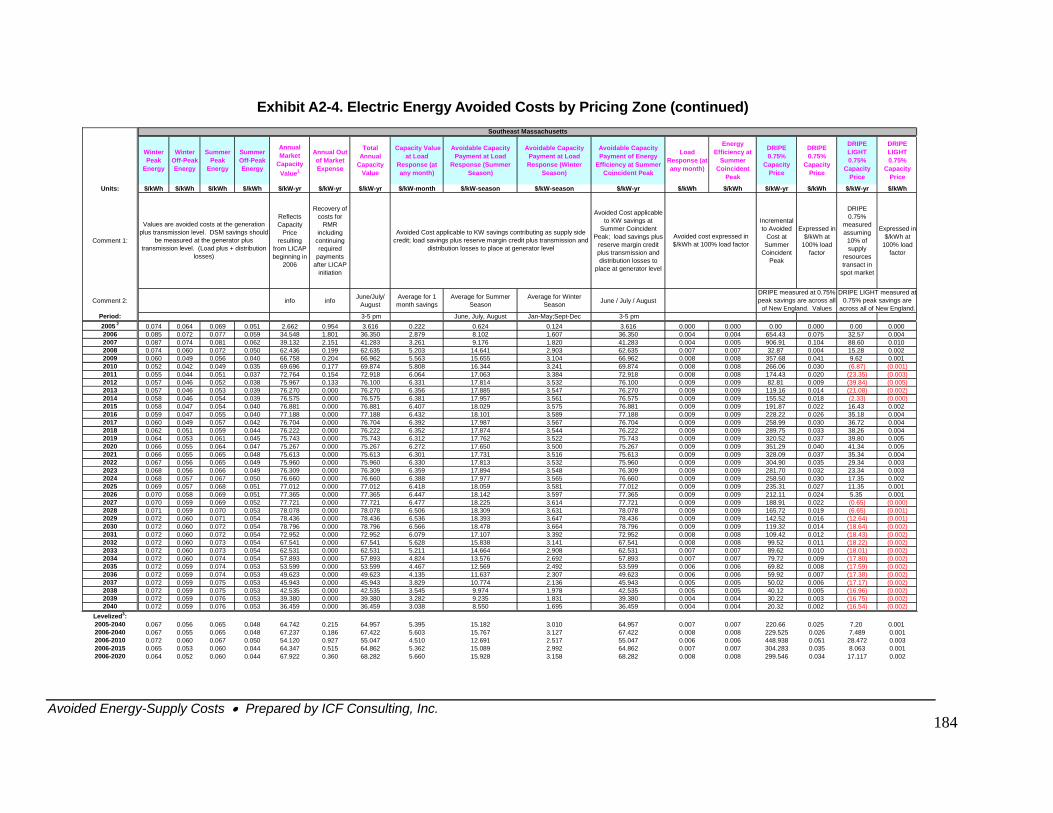
Exhibit A2-4. Electric Energy Avoided Costs by Pricing Zone (continued)
Winter Peak
Energy
Winter Off-Peak Energy
Summer Peak
Energy
Summer Off-Peak Energy
Annual Market
Capacity Value1
Annual Out of Market Expense
Total Annual
Capacity Value
Capacity Value at Load
Response (at any month)
Avoidable Capacity Payment at Load
Response (Summer Season)
Avoidable Capacity Payment at Load Response (Winter
Season)
Avoidable Capacity Payment of Energy
Efficiency at Summer Coincident Peak
Load Response (at any month)
Energy Efficiency at
Summer Coincident
Peak
DRIPE 0.75%
Capacity Price
DRIPE 0.75%
Capacity Price
DRIPE LIGHT 0.75%
Capacity Price
DRIPE LIGHT 0.75%
Capacity Price
Units: $/kWh $/kWh $/kWh $/kWh $/kW-yr $/kW-yr $/kW-yr $/kW-month $/kW-season $/kW-season $/kW-yr $/kWh $/kWh $/kW-yr $/kWh $/kW-yr $/kWh
Comment 1:
Reflects Capacity
Price resulting
from LICAP beginning in
2006
Recovery of costs for
RMR including
continuing required
payments after LICAP
initiation
Avoided Cost applicable to KW savings at
Summer Coincident Peak; load savings plus
reserve margin credit plus transmission and distribution losses to
place at generator level
Incremental to Avoided
Cost at Summer
Coincident Peak
Expressed in $/kWh at
100% load factor
DRIPE 0.75%
measured assuming
10% of supply
resources transact in
spot market
Expressed in $/kWh at
100% load factor
Comment 2: info info June/July/ August
Average for 1 month savings
Average for Summer Season
Average for Winter Season June / July / August
Period: 3-5 pm June, July, August Jan-May;Sept-Dec 3-5 pm2005 2 0.074 0.064 0.069 0.051 2.662 0.954 3.616 0.222 0.624 0.124 3.616 0.000 0.000 0.00 0.000 0.00 0.0002006 0.085 0.072 0.077 0.059 34.548 1.801 36.350 2.879 8.102 1.607 36.350 0.004 0.004 654.43 0.075 32.57 0.0042007 0.087 0.074 0.081 0.062 39.132 2.151 41.283 3.261 9.176 1.820 41.283 0.004 0.005 906.91 0.104 88.60 0.0102008 0.074 0.060 0.072 0.050 62.436 0.199 62.635 5.203 14.641 2.903 62.635 0.007 0.007 32.87 0.004 15.28 0.0022009 0.060 0.049 0.056 0.040 66.758 0.204 66.962 5.563 15.655 3.104 66.962 0.008 0.008 357.68 0.041 9.62 0.0012010 0.052 0.042 0.049 0.035 69.696 0.177 69.874 5.808 16.344 3.241 69.874 0.008 0.008 266.06 0.030 (0.2011 0.055 0.044 0.051 0.037 72.764 0.154 72.918 6.064 17.063 3.384 72.918 0.008 0.008 174.43 0.020 (2 (0.2012 0.057 0.046 0.052 0.038 75.967 0.133 76.100 6.331 17.814 3.532 76.100 0.009 0.009 82.81 0.009 (3 (0.2013 0.057 0.046 0.053 0.039 76.270 0.000 76.270 6.356 17.885 3.547 76.270 0.009 0.009 119.16 0.014 (2 (0.2014 0.058 0.046 0.054 0.039 76.575 0.000 76.575 6.381 17.957 3.561 76.575 0.009 0.009 155.52 0.018 (0.2015 0.058 0.047 0.054 0.040 76.881 0.000 76.881 6.407 18.029 3.575 76.881 0.009 0.009 191.87 0.022 02016 0.059 0.047 0.055 0.040 77.188 0.000 77.188 6.432 18.101 3.589 77.188 0.009 0.009 228.22 0.026 35 02017 0.060 0.049 0.057 0.042 76.704 0.000 76.704 6.392 17.987 3.567 76.704 0.009 0.009 258.99 0.030 36 02018 0.062 0.051 0.059 0.044 76.222 0.000 76.222 6.352 17.874 3.544 76.222 0.009 0.009 289.75 0.033 38 02019 0.064 0.053 0.061 0.045 75.743 0.000 75.743 6.312 17.762 3.522 75.743 0.009 0.009 320.52 0.037 39 02020 0.066 0.055 0.064 0.047 75.267 0.000 75.267 6.272 17.650 3.500 75.267 0.009 0.009 351.29 0.040 41 02021 0.066 0.055 0.065 0.048 75.613 0.000 75.613 6.301 17.731 3.516 75.613 0.009 0.009 328.09 0.037 35 02022 0.067 0.056 0.065 0.049 75.960 0.000 75.960 6.330 17.813 3.532 75.960 0.009 0.009 304.90 0.035 29 02023 0.068 0.056 0.066 0.049 76.309 0.000 76.309 6.359 17.894 3.548 76.309 0.009 0.009 281.70 0.032 23 02024 0.068 0.057 0.067 0.050 76.660 0.000 76.660 6.388 17.977 3.565 76.660 0.009 0.009 258.50 0.030 17 02025 0.069 0.057 0.068 0.051 77.012 0.000 77.012 6.418 18.059 3.581 77.012 0.009 0.009 235.31 0.027 02026 0.070 0.058 0.069 0.051 77.365 0.000 77.365 6.447 18.142 3.597 77.365 0.009 0.009 212.11 0.024 0.2027 0.070 0.059 0.069 0.052 77.721 0.000 77.721 6.477 18.225 3.614 77.721 0.009 0.009 188.91 0.022 (0.2028 0.071 0.059 0.070 0.053 78.078 0.000 78.078 6.506 18.309 3.631 78.078 0.009 0.009 165.72 0.019 (0.2029 0.072 0.060 0.071 0.054 78.436 0.000 78.436 6.536 18.393 3.647 78.436 0.009 0.009 142.52 0.016 (1 (0.2030 0.072 0.060 0.072 0.054 78.796 0.000 78.796 6.566 18.478 3.664 78.796 0.009 0.009 119.32 0.014 (1 (0.2031 0.072 0.060 0.072 0.054 72.952 0.000 72.952 6.079 17.107 3.392 72.952 0.008 0.008 109.42 0.012 (1 (0.2032 0.072 0.060 0.073 0.054 67.541 0.000 67.541 5.628 15.838 3.141 67.541 0.008 0.008 99.52 0.011 (1 (0.2033 0.072 0.060 0.073 0.054 62.531 0.000 62.531 5.211 14.664 2.908 62.531 0.007 0.007 89.62 0.010 (1 (0.2034 0.072 0.060 0.074 0.054 57.893 0.000 57.893 4.824 13.576 2.692 57.893 0.007 0.007 79.72 0.009 (1 (0.2035 0.072 0.059 0.074 0.053 53.599 0.000 53.599 4.467 12.569 2.492 53.599 0.006 0.006 69.82 0.008 (1 (0.2036 0.072 0.059 0.074 0.053 49.623 0.000 49.623 4.135 11.637 2.307 49.623 0.006 0.006 59.92 0.007 (1 (0.2037 0.072 0.059 0.075 0.053 45.943 0.000 45.943 3.829 10.774 2.136 45.943 0.005 0.005 50.02 0.006 (1 (0.2038 0.072 0.059 0.075 0.053 42.535 0.000 42.535 3.545 9.974 1.978 42.535 0.005 0.005 40.12 0.005 (1 (0.2039 0.072 0.059 0.076 0.053 39.380 0.000 39.380 3.282 9.235 1.831 39.380 0.004 0.004 30.22 0.003 (16. (0.2040 0.072 0.059 0.076 0.053 36.459 0.000 36.459 3.038 8.550 1.695 36.459 0.004 0.004 20.32 0.002 (16 (0.
Levelized3: 2005-2040 0.067 0.056 0.065 0.048 64.742 0.215 64.957 5.395 15.182 3.010 64.957 0.007 0.007 220.66 0.025 7.20 0.0012006-2040 0.067 0.055 0.065 0.048 67.237 0.186 67.422 5.603 15.767 3.127 67.422 0.008 0.008 229.525 0.026 7.489 0.0012006-2010 0.072 0.060 0.067 0.050 54.120 0.927 55.047 4.510 12.691 2.517 55.047 0.006 0.006 448.938 0.051 28.472 0.0032006-2015 0.065 0.053 0.060 0.044 64.347 0.515 64.862 5.362 15.089 2.992 64.862 0.007 0.007 304.283 0.035 8.063 0.0012006-2020 0.064 0.052 0.060 0.044 67.922 0.360 68.282 5.660 15.928 3.158 68.282 0.008 0.008 299.546 0.034 17.117 0.002
Southeast Massachusetts
DRIPE LIGHT measured at 0.75% peak savings are
across all of New England.
DRIPE measured at 0.75% peak savings are across all
of New England. Values
Avoided cost expressed in $/kWh at 100% load factor
Values are avoided costs at the generation plus transmission level. DSM savings should
be measured at the generator plus transmission level. (Load plus + distribution
losses)
Avoided Cost applicable to KW savings contributing as supply side credit; load savings plus reserve margin credit plus transmission and
distribution losses to place at generator level
(6.87) 001)3.35) 003)9.84) 005)1.08) 002)
(2.33) 000)16.43 .002
.18 .004
.72 .004
.26 .004
.80 .005
.34 .005
.34 .004
.34 .003
.34 .003
.35 .00211.35 .0015.35 001(0.65) 000)(6.65) 001)
2.64) 001)8.64) 002)8.43) 002)8.22) 002)8.01) 002)7.80) 002)7.59) 002)7.38) 002)7.17) 002)6.96) 002)
75) 002).54) 002)
Avoided Energy-Supply Costs • Prepared by ICF Consulting, Inc.
184
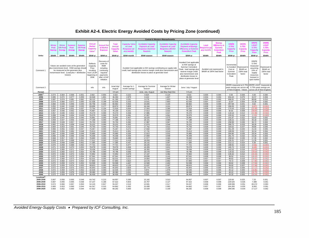
Avoided Energy-Supply Costs • Prepared by ICF Consulting, Inc.
185
Exhibit A2-4. Electric Energy Avoided Costs by Pricing Zone (continued)
Winter Peak
Energy
Winter Off-Peak Energy
Summer Peak
Energy
Summer Off-Peak Energy
Annual Market
Capacity Value1
Annual Out of Market Expense
Total Annual
Capacity Value
Capacity Value at Load
Response (at any month)
Avoidable Capacity Payment at Load
Response (Summer Season)
Avoidable Capacity Payment at Load Response (Winter
Season)
Avoidable Capacity Payment of Energy
Efficiency at Summer Coincident Peak
Load Response (at any month)
Energy Efficiency at
Summer Coincident
Peak
DRIPE 0.75%
Capacity Price
DRIPE 0.75%
Capacity Price
DRIPE LIGHT 0.75%
Capacity Price
DRIPE LIGHT 0.75%
Capacity Price
Units: $/kWh $/kWh $/kWh $/kWh $/kW-yr $/kW-yr $/kW-yr $/kW-month $/kW-season $/kW-season $/kW-yr $/kWh $/kWh $/kW-yr $/kWh $/kW-yr $/kWh
Comment 1:
Reflects Capacity
Price resulting
from LICAP beginning in
2006
Recovery of costs for
RMR including
continuing required
payments after LICAP
initiation
Avoided Cost applicable to KW savings at
Summer Coincident Peak; load savings plus
reserve margin credit plus transmission and distribution losses to
place at generator level
Incremental to Avoided
Cost at Summer
Coincident Peak
Expressed in $/kWh at
100% load factor
DRIPE 0.75%
measured assuming
10% of supply
resources transact in
spot market
Expressed in$/kWh at
100% load factor
Comment 2: info info June/July/ August
Average for 1 month savings
Average for Summer Season
Average for Winter Season June / July / August
Period: 3-5 pm June, July, August Jan-May;Sept-Dec 3-5 pm2005 2 0.074 0.064 0.069 0.051 2.662 0.954 3.616 0.222 0.624 0.124 3.616 0.000 0.000 0.00 0.000 0.00 0.0002006 0.085 0.072 0.077 0.059 34.548 1.801 36.350 2.879 8.102 1.607 36.350 0.004 0.004 654.43 0.075 32.57 0.0042007 0.087 0.074 0.081 0.062 39.132 2.151 41.283 3.261 9.176 1.820 41.283 0.004 0.005 906.91 0.104 88.60 0.0102008 0.074 0.060 0.072 0.050 62.436 0.199 62.635 5.203 14.641 2.903 62.635 0.007 0.007 32.87 0.004 15.28 0.0022009 0.060 0.049 0.056 0.040 66.758 0.204 66.962 5.563 15.655 3.104 66.962 0.008 0.008 357.68 0.041 9.62 0.0012010 0.052 0.042 0.049 0.035 69.696 0.177 69.874 5.808 16.344 3.241 69.874 0.008 0.008 266.06 0.030
87) 01)2011 0.055 0.044 0.051 0.037 72.764 0.154 72.918 6.064 17.063 3.384 72.918 0.008 0.008 174.43 0.020 35) 3)2012 0.057 0.046 0.052 0.038 75.967 0.133 76.100 6.331 17.814 3.532 76.100 0.009 0.009 82.81 0.009 4) 5)2013 0.057 0.046 0.053 0.039 76.270 0.000 76.270 6.356 17.885 3.547 76.270 0.009 0.009 119.16 0.014 8) 2)2014 0.058 0.046 0.054 0.039 76.575 0.000 76.575 6.381 17.957 3.561 76.575 0.009 0.009 155.52 0.018 3) 0)2015 0.058 0.047 0.054 0.040 76.881 0.000 76.881 6.407 18.029 3.575 76.881 0.009 0.009 191.87 0.022 32016 0.059 0.047 0.055 0.040 77.188 0.000 77.188 6.432 18.101 3.589 77.188 0.009 0.009 228.22 0.026 35.18 0.0042017 0.060 0.049 0.057 0.042 76.704 0.000 76.704 6.392 17.987 3.567 76.704 0.009 0.009 258.99 0.030 36.72 0.0042018 0.062 0.051 0.059 0.044 76.222 0.000 76.222 6.352 17.874 3.544 76.222 0.009 0.009 289.75 0.033 38.26 0.0042019 0.064 0.053 0.061 0.045 75.743 0.000 75.743 6.312 17.762 3.522 75.743 0.009 0.009 320.52 0.037 39.80 0.0052020 0.066 0.055 0.064 0.047 75.267 0.000 75.267 6.272 17.650 3.500 75.267 0.009 0.009 351.29 0.040 41.34 0.0052021 0.066 0.055 0.065 0.048 75.613 0.000 75.613 6.301 17.731 3.516 75.613 0.009 0.009 328.09 0.037 35.34 0.0042022 0.067 0.056 0.065 0.049 75.960 0.000 75.960 6.330 17.813 3.532 75.960 0.009 0.009 304.90 0.035 29.34 0.0032023 0.068 0.056 0.066 0.049 76.309 0.000 76.309 6.359 17.894 3.548 76.309 0.009 0.009 281.70 0.032 23.34 0.0032024 0.068 0.057 0.067 0.050 76.660 0.000 76.660 6.388 17.977 3.565 76.660 0.009 0.009 258.50 0.030 17.35 0.0022025 0.069 0.057 0.068 0.051 77.012 0.000 77.012 6.418 18.059 3.581 77.012 0.009 0.009 235.31 0.027 11.35 0.0012026 0.070 0.058 0.069 0.051 77.365 0.000 77.365 6.447 18.142 3.597 77.365 0.009 0.009 212.11 0.024 5.35 0.0012027 0.070 0.059 0.069 0.052 77.721 0.000 77.721 6.477 18.225 3.614 77.721 0.009 0.009 188.91 0.022 (0.65) (0.000)2028 0.071 0.059 0.070 0.053 78.078 0.000 78.078 6.506 18.309 3.631 78.078 0.009 0.009 165.72 0.019 5) 1)2029 0.072 0.060 0.071 0.054 78.436 0.000 78.436 6.536 18.393 3.647 78.436 0.009 0.009 142.52 0.016 64) 1)2030 0.072 0.060 0.072 0.054 78.796 0.000 78.796 6.566 18.478 3.664 78.796 0.009 0.009 119.32 0.014 4) 2)2031 0.072 0.060 0.072 0.054 72.952 0.000 72.952 6.079 17.107 3.392 72.952 0.008 0.008 109.42 0.012 3) 2)2032 0.072 0.060 0.073 0.054 67.541 0.000 67.541 5.628 15.838 3.141 67.541 0.008 0.008 99.52 0.011 2) 2)2033 0.072 0.060 0.073 0.054 62.531 0.000 62.531 5.211 14.664 2.908 62.531 0.007 0.007 89.62 0.010 1) 2)2034 0.072 0.060 0.074 0.054 57.893 0.000 57.893 4.824 13.576 2.692 57.893 0.007 0.007 79.72 0.009 0) 2)2035 0.072 0.059 0.074 0.053 53.599 0.000 53.599 4.467 12.569 2.492 53.599 0.006 0.006 69.82 0.008 9) 2)2036 0.072 0.059 0.074 0.053 49.623 0.000 49.623 4.135 11.637 2.307 49.623 0.006 0.006 59.92 0.007 8) 2)2037 0.072 0.059 0.075 0.053 45.943 0.000 45.943 3.829 10.774 2.136 45.943 0.005 0.005 50.02 0.006 7) 2)2038 0.072 0.059 0.075 0.053 42.535 0.000 42.535 3.545 9.974 1.978 42.535 0.005 0.005 40.12 0.005 6) 2)2039 0.072 0.059 0.076 0.053 39.380 0.000 39.380 3.282 9.235 1.831 39.380 0.004 0.004 30.22 0.003 5) 2)2040 0.072 0.059 0.076 0.053 36.459 0.000 36.459 3.038 8.550 1.695 36.459 0.004 0.004 20.32 0.002 4) 2)
Levelized3: 2005-2040 0.067 0.056 0.065 0.048 64.742 0.215 64.957 5.395 15.182 3.010 64.957 0.007 0.007 220.66 0.0252006-2040 0.067 0.055 0.065 0.048 67.237 0.186 67.422 5.603 15.767 3.127 67.422 0.008 0.008 229.525 0.026 7.489 0.0012006-2010 0.072 0.060 0.067 0.050 54.120 0.927 55.047 4.510 12.691 2.517 55.047 0.006 0.006 448.938 0.051 28.472 0.0032006-2015 0.065 0.053 0.060 0.044 64.347 0.515 64.862 5.362 15.089 2.992 64.862 0.007 0.007 304.283 0.035 8.063 0.0012006-2020 0.064 0.052 0.060 0.044 67.922 0.360 68.282 5.660 15.928 3.158 68.282 0.008 0.008 299.546 0.034 17.117 0.002
Central & Western Massachusetts
DRIPE LIGHT measured at 0.75% peak savings are
across all of New England.
DRIPE measured at 0.75% peak savings are across all
of New England. Values
Avoided Cost applicable to KW savings contributing as supply side credit; load savings plus reserve margin credit plus transmission and
distribution losses to place at generator level
Values are avoided costs at the generation plus transmission level. DSM savings should
be measured at the generator plus transmission level. (Load plus + distribution
losses)
Avoided cost expressed in $/kWh at 100% load factor
(6. (0.0(23. (0.00(39.8 (0.00(21.0 (0.00(2.3 (0.0016.4 0.002
(6.6 (0.00(12. (0.00(18.6 (0.00(18.4 (0.00(18.2 (0.00(18.0 (0.00(17.8 (0.00(17.5 (0.00(17.3 (0.00(17.1 (0.00(16.9 (0.00(16.7 (0.00(16.5 (0.00
7.20 0.001
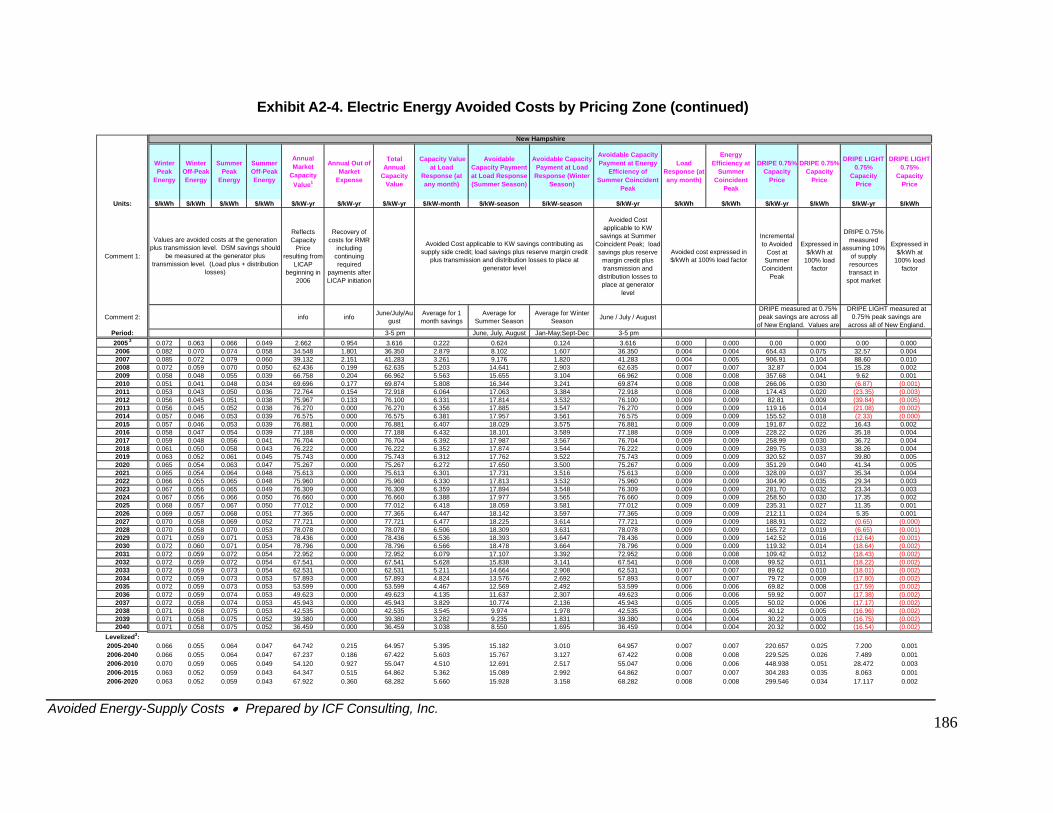
Avoided Energy-Supply Costs • Prepared by ICF Consulting, Inc.
186
Exhibit A2-4. Electric Energy Avoided Costs by Pricing Zone (continued)
Winter Peak
Energy
Winter Off-Peak Energy
Summer Peak
Energy
Summer Off-Peak Energy
Annual Market
Capacity Value1
Annual Out of Market
Expense
Total Annual
Capacity Value
Capacity Value at Load
Response (at any month)
Avoidable Capacity Payment at Load Response (Summer Season)
Avoidable Capacity Payment at Load Response (Winter
Season)
Avoidable Capacity Payment at Energy
Efficiency of Summer Coincident
Peak
Load Response (at any month)
Energy Efficiency at
Summer Coincident
Peak
DRIPE 0.75% Capacity
Price
DRIPE 0.75% Capacity
Price
DRIPE LIGHT 0.75%
Capacity Price
DRIPE LIGHT0.75%
Capacity Price
Units: $/kWh $/kWh $/kWh $/kWh $/kW-
yr $/kW-yr $/kW-yr $/kW-month $/kW-season $/kW-season $/kW-yr $/kWh $/kWh $/kW-yr $/kWh $/kW-yr $/kWh
omment 1:
Reflects Capacity
Price resulting from
LICAP beginning in
2006
Recovery of costs for RMR
including continuing required
payments after LICAP initiation
Avoided Cost applicable to KW
savings at Summer Coincident Peak; load savings plus reserve
margin credit plus transmission and
distribution losses to place at generator
level
Incremental to Avoided
Cost at Summer
Coincident Peak
Expressed in $/kWh at
100% load factor
DRIPE 0.75% measured
assuming 10% of supply resources transact in
spot market
Expressed in $/kWh at
100% load factor
omment 2: info info June/July/August
Average for 1 month savings
Average for Summer Season
Average for Winter Season June / July / August
Period: 3-5 pm June, July, August Jan-May;Sept-Dec 3-5 pm2005 2 0.072 0.063 0.066 0.049 2.662 0.954 3.616 0.222 0.624 0.124 3.616 0.000 0.000 0.00 0.000 0.00 0.0002006 0.082 0.070 0.074 0.058 34.548 1.801 36.350 2.879 8.102 1.607 36.350 0.004 0.004 654.43 0.075 32.57 0.0042007 0.085 0.072 0.079 0.060 39.132 2.151 41.283 3.261 9.176 1.820 41.283 0.004 0.005 906.91 0.104 8
C
C
2008 0.072 0.059 0.070 0.050 62.436 0.199 62.635 5.203 14.641 2.903 62.635 0.007 0.007 32.87 0.0042009 0.058 0.048 0.055 0.039 66.758 0.204 66.962 5.563 15.655 3.104 66.962 0.008 0.008 357.68 0.0412010 0.051 0.041 0.048 0.034 69.696 0.177 69.874 5.808 16.344 3.241 69.874 0.008 0.008 266.06 0.0302011 0.053 0.043 0.050 0.036 72.764 0.154 72.918 6.064 17.063 3.384 72.918 0.008 0.008 174.43 0.0202012 0.056 0.045 0.051 0.038 75.967 0.133 76.100 6.331 17.814 3.532 76.100 0.009 0.009 82.81 0.009 (32013 0.056 0.045 0.052 0.038 76.270 0.000 76.270 6.356 17.885 3.547 76.270 0.009 0.009 119.16 0.014 (21.08) (0.002)2014 0.057 0.046 0.053 0.039 76.575 0.000 76.575 6.381 17.957 3.561 76.575 0.009 0.009 155.52 0.018 (2.33) (0.000)2015 0.057 0.046 0.053 0.039 76.881 0.000 76.881 6.407 18.029 3.575 76.881 0.009 0.009 191.87 0.022 16.43 0.0022016 0.058 0.047 0.054 0.039 77.188 0.000 77.188 6.432 18.101 3.589 77.188 0.009 0.009 228.22 0.026 35.18 0.0042017 0.059 0.048 0.056 0.041 76.704 0.000 76.704 6.392 17.987 3.567 76.704 0.009 0.009 258.99 0.030 36.72 0.0042018 0.061 0.050 0.058 0.043 76.222 0.000 76.222 6.352 17.874 3.544 76.222 0.009 0.009 289.75 0.033 38.26 0.0042019 0.063 0.052 0.061 0.045 75.743 0.000 75.743 6.312 17.762 3.522 75.743 0.009 0.009 320.52 0.037 39.80 0.0052020 0.065 0.054 0.063 0.047 75.267 0.000 75.267 6.272 17.650 3.500 75.267 0.009 0.009 351.29 0.040 41.34 0.0052021 0.065 0.054 0.064 0.048 75.613 0.000 75.613 6.301 17.731 3.516 75.613 0.009 0.009 328.09 0.037 35.34 0.0042022 0.066 0.055 0.065 0.048 75.960 0.000 75.960 6.330 17.813 3.532 75.960 0.009 0.009 304.90 0.035 29.34 0.0032023 0.067 0.056 0.065 0.049 76.309 0.000 76.309 6.359 17.894 3.548 76.309 0.009 0.009 281.70 0.032 23.34 0.0032024 0.067 0.056 0.066 0.050 76.660 0.000 76.660 6.388 17.977 3.565 76.660 0.009 0.009 258.50 0.0302025 0.068 0.057 0.067 0.050 77.012 0.000 77.012 6.418 18.059 3.581 77.012 0.009 0.009 235.31 0.0272026 0.069 0.057 0.068 0.051 77.365 0.000 77.365 6.447 18.142 3.597 77.365 0.009 0.009 212.11 0.0242027 0.070 0.058 0.069 0.052 77.721 0.000 77.721 6.477 18.225 3.614 77.721 0.009 0.009 188.91 0.0222028 0.070 0.058 0.070 0.053 78.078 0.000 78.078 6.506 18.309 3.631 78.078 0.009 0.009 165.72 0.0192029 0.071 0.059 0.071 0.053 78.436 0.000 78.436 6.536 18.393 3.647 78.436 0.009 0.009 142.52 0.0162030 0.072 0.060 0.071 0.054 78.796 0.000 78.796 6.566 18.478 3.664 78.796 0.009 0.009 119.32 0.0142031 0.072 0.059 0.072 0.054 72.952 0.000 72.952 6.079 17.107 3.392 72.952 0.008 0.008 109.42 0.0122032 0.072 0.059 0.072 0.054 67.541 0.000 67.541 5.628 15.838 3.141 67.541 0.008 0.008 99.52 0.0112033 0.072 0.059 0.073 0.054 62.531 0.000 62.531 5.211 14.664 2.908 62.531 0.007 0.007 89.62 0.0102034 0.072 0.059 0.073 0.053 57.893 0.000 57.893 4.824 13.576 2.692 57.893 0.007 0.007 79.72 0.0092035 0.072 0.059 0.073 0.053 53.599 0.000 53.599 4.467 12.569 2.492 53.599 0.006 0.006 69.82 0.0082036 0.072 0.059 0.074 0.053 49.623 0.000 49.623 4.135 11.637 2.307 49.623 0.006 0.006 59.92 0.0072037 0.072 0.058 0.074 0.053 45.943 0.000 45.943 3.829 10.774 2.136 45.943 0.005 0.005 50.02 0.0062038 0.071 0.058 0.075 0.053 42.535 0.000 42.535 3.545 9.974 1.978 42.535 0.005 0.005 40.12 0.005 (16.96) (0.002)2039 0.071 0.058 0.075 0.052 39.380 0.000 39.380 3.282 9.235 1.831 39.380 0.004 0.004 30.22 0.003 (16.75) (0.002)2040 0.071 0.058 0.075 0.052 36.459 0.000 36.459 3.038 8.550 1.695 36.459 0.004 0.004 20.32 0.002 (16.54) (0.002)
Levelized3: 2005-2040 0.066 0.055 0.064 0.047 64.742 0.215 64.957 5.395 15.182 3.010 64.957 0.007 0.007 220.657 0.025 7.200 0.0012006-2040 0.066 0.055 0.064 0.047 67.237 0.186 67.422 5.603 15.767 3.127 67.422 0.008 0.008 229.525 0.026 7.489 0.0012006-2010 0.070 0.059 0.065 0.049 54.120 0.927 55.047 4.510 12.691 2.517 55.047 0.006 0.006 448.938 0.051 28.472 0.0032006-2015 0.063 0.052 0.059 0.043 64.347 0.515 64.862 5.362 15.089 2.992 64.862 0.007 0.007 304.283 0.035 8.063 0.0012006-2020 0.063 0.052 0.059 0.043 67.922 0.360 68.282 5.660 15.928 3.158 68.282 0.008 0.008 299.546 0.034 17.117 0.002
New Hampshire
Values are avoided costs at the generation plus transmission level. DSM savings should
be measured at the generator plus transmission level. (Load plus + distribution
losses)
Avoided cost expressed in $/kWh at 100% load factor
DRIPE measured at 0.75% peak savings are across all
of New England. Values are
DRIPE LIGHT measured at 0.75% peak savings are
across all of New England.
Avoided Cost applicable to KW savings contributing as supply side credit; load savings plus reserve margin credit
plus transmission and distribution losses to place at generator level
8.60 0.01015.28 0.0029.62 0.001(6.87) (0.001)(23.35) (0.003)
9.84) (0.005)
17.35 0.00211.35 0.0015.35 0.001(0.65) (0.000)(6.65) (0.001)(12.64) (0.001)(18.64) (0.002)(18.43) (0.002)(18.22) (0.002)(18.01) (0.002)(17.80) (0.002)(17.59) (0.002)(17.38) (0.002)(17.17) (0.002)
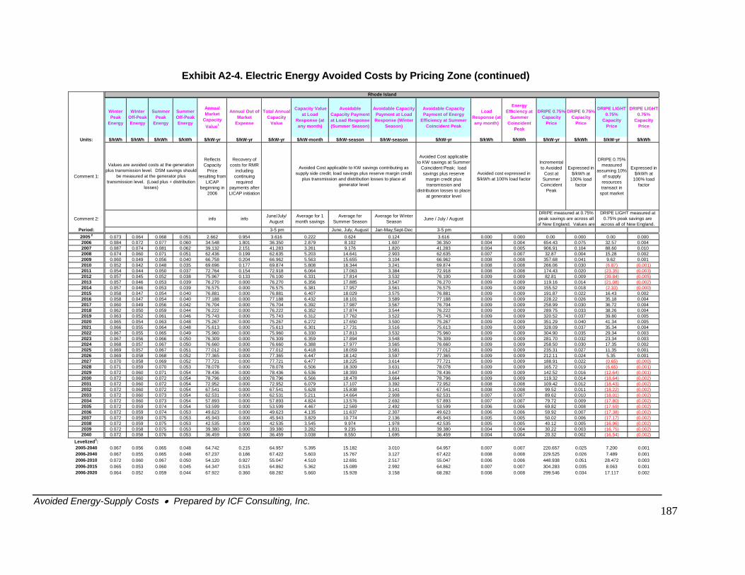
Avoided Energy-Supply Costs • Prepared by ICF Consulting, Inc.
187
Exhibit A2-4. Electric Energy Avoided Costs by Pricing Zone (continued)
Winter Peak
Energy
Winter Off-Peak Energy
Summer Peak
Energy
Summer Off-Peak Energy
Annual Market
Capacity Value1
Annual Out of Market
Expense
Total Annual Capacity
Value
Capacity Value at Load
Response (at any month)
Avoidable Capacity Payment at Load Response (Summer Season)
Avoidable Capacity Payment at Load Response (Winter
Season)
Avoidable Capacity Payment of Energy
Efficiency at Summer Coincident Peak
Load Response (at any month)
Energy Efficiency at
Summer Coincident
Peak
DRIPE 0.75% Capacity
Price
DRIPE 0.75% Capacity
Price
DRIPE LIGHT 0.75%
Capacity Price
DRIPE LIGHT 0.75%
Capacity Price
Units: $/kWh $/kWh $/kWh $/kWh $/kW-yr $/kW-yr $/kW-yr $/kW-month $/kW-season $/kW-season $/kW-yr $/kWh $/kWh $/kW-yr $/kWh $/kW-yr $/kWh
Comment 1:
Reflects Capacity
Price resulting from
LICAP beginning in
2006
Recovery of costs for RMR
including continuing required
payments after LICAP initiation
Avoided Cost applicable to KW savings at Summer
Coincident Peak; load savings plus reserve
margin credit plus transmission and
distribution losses to place at generator level
Incremental to Avoided
Cost at Summer
Coincident Peak
Expressed in $/kWh at
100% load factor
DRIPE 0.75% measured
assuming 10% of supply resources transact in
spot market
Expressed in $/kWh at
100% load factor
Comment 2: info info June/July/ August
Average for 1 month savings
Average for Summer Season
Average for Winter Season June / July / August
Period: 3-5 pm June, July, August Jan-May;Sept-Dec 3-5 pm2005 2 0.073 0.064 0.068 0.051 2.662 0.954 3.616 0.222 0.624 0.124 3.616 0.000 0.000 0.00 0.000 0.00 0.0002006 0.084 0.072 0.077 0.060 34.548 1.801 36.350 2.879 8.102 1.607 36.350 0.004 0.004 654.43 0.075 32.57 0.0042007 0.087 0.074 0.081 0.062 39.132 2.151 41.283 3.261 9.176 1.820 41.283 0.004 0.005 906.91 0.104 88.60 0.0102008 0.074 0.060 0.071 0.051 62.436 0.199 62.635 5.203 14.641 2.903 62.635 0.007 0.007 32.87 0.004 15.28 0.0022009 0.060 0.049 0.056 0.040 66.758 0.204 66.962 5.563 15.655 3.104 66.962 0.008 0.008 357.68 0.041 9.62 0.0012010 0.052 0.042 0.048 0.035 69.696 0.177 69.874 5.808 16.344 3.241 69.874 0.008 0.008 266.06 0.030 (6.87) (0.001)2011 0.054 0.044 0.050 0.037 72.764 0.154 72.918 6.064 17.063 3.384 72.918 0.008 0.008 174.43 0.020 (23.35) (0.003)
(39.84) (0.005)(21.08) (0.002)(2.33) (0.000)16.43 0.00235.18 0.004
(6.65) (0.001)(12.64) (0.001)(18.64) (0.002)(18.43) (0.002)(18.22) (0.002)(18.01) (0.002)(17.80) (0.002)(17.59) (0.002)(17.38) (0.002)(17.17) (0.002)(16.96) (0.002)(16.75) (0.002)(16.54) (0.002)
7.200 0.001
2012 0.057 0.045 0.052 0.038 75.967 0.133 76.100 6.331 17.814 3.532 76.100 0.009 0.009 82.81 0.0092013 0.057 0.046 0.053 0.039 76.270 0.000 76.270 6.356 17.885 3.547 76.270 0.009 0.009 119.16 0.0142014 0.057 0.046 0.053 0.039 76.575 0.000 76.575 6.381 17.957 3.561 76.575 0.009 0.009 155.52 0.0182015 0.058 0.047 0.054 0.040 76.881 0.000 76.881 6.407 18.029 3.575 76.881 0.009 0.009 191.87 0.0222016 0.058 0.047 0.054 0.040 77.188 0.000 77.188 6.432 18.101 3.589 77.188 0.009 0.009 228.22 0.0262017 0.060 0.049 0.056 0.042 76.704 0.000 76.704 6.392 17.987 3.567 76.704 0.009 0.009 258.99 0.030 36.72 0.0042018 0.062 0.050 0.059 0.044 76.222 0.000 76.222 6.352 17.874 3.544 76.222 0.009 0.009 289.75 0.033 38.26 0.0042019 0.063 0.052 0.061 0.046 75.743 0.000 75.743 6.312 17.762 3.522 75.743 0.009 0.009 320.52 0.037 39.80 0.0052020 0.065 0.054 0.063 0.048 75.267 0.000 75.267 6.272 17.650 3.500 75.267 0.009 0.009 351.29 0.040 41.34 0.0052021 0.066 0.055 0.064 0.048 75.613 0.000 75.613 6.301 17.731 3.516 75.613 0.009 0.009 328.09 0.037 35.34 0.0042022 0.067 0.055 0.065 0.049 75.960 0.000 75.960 6.330 17.813 3.532 75.960 0.009 0.009 304.90 0.035 29.34 0.0032023 0.067 0.056 0.066 0.050 76.309 0.000 76.309 6.359 17.894 3.548 76.309 0.009 0.009 281.70 0.032 23.34 0.0032024 0.068 0.057 0.067 0.050 76.660 0.000 76.660 6.388 17.977 3.565 76.660 0.009 0.009 258.50 0.030 17.35 0.0022025 0.069 0.057 0.067 0.051 77.012 0.000 77.012 6.418 18.059 3.581 77.012 0.009 0.009 235.31 0.027 11.35 0.0012026 0.069 0.058 0.068 0.052 77.365 0.000 77.365 6.447 18.142 3.597 77.365 0.009 0.009 212.11 0.024 5.35 0.0012027 0.070 0.058 0.069 0.052 77.721 0.000 77.721 6.477 18.225 3.614 77.721 0.009 0.009 188.91 0.022 (0.65) (0.000)2028 0.071 0.059 0.070 0.053 78.078 0.000 78.078 6.506 18.309 3.631 78.078 0.009 0.009 165.72 0.0192029 0.072 0.060 0.071 0.054 78.436 0.000 78.436 6.536 18.393 3.647 78.436 0.009 0.009 142.52 0.0162030 0.072 0.060 0.072 0.054 78.796 0.000 78.796 6.566 18.478 3.664 78.796 0.009 0.009 119.32 0.0142031 0.072 0.060 0.072 0.054 72.952 0.000 72.952 6.079 17.107 3.392 72.952 0.008 0.008 109.42 0.0122032 0.072 0.060 0.072 0.054 67.541 0.000 67.541 5.628 15.838 3.141 67.541 0.008 0.008 99.52 0.0112033 0.072 0.060 0.073 0.054 62.531 0.000 62.531 5.211 14.664 2.908 62.531 0.007 0.007 89.62 0.0102034 0.072 0.060 0.073 0.054 57.893 0.000 57.893 4.824 13.576 2.692 57.893 0.007 0.007 79.72 0.0092035 0.072 0.059 0.074 0.054 53.599 0.000 53.599 4.467 12.569 2.492 53.599 0.006 0.006 69.82 0.0082036 0.072 0.059 0.074 0.053 49.623 0.000 49.623 4.135 11.637 2.307 49.623 0.006 0.006 59.92 0.0072037 0.072 0.059 0.075 0.053 45.943 0.000 45.943 3.829 10.774 2.136 45.943 0.005 0.005 50.02 0.0062038 0.072 0.059 0.075 0.053 42.535 0.000 42.535 3.545 9.974 1.978 42.535 0.005 0.005 40.12 0.0052039 0.072 0.058 0.075 0.053 39.380 0.000 39.380 3.282 9.235 1.831 39.380 0.004 0.004 30.22 0.0032040 0.072 0.058 0.076 0.053 36.459 0.000 36.459 3.038 8.550 1.695 36.459 0.004 0.004 20.32 0.002
Levelized3: 2005-2040 0.067 0.056 0.065 0.048 64.742 0.215 64.957 5.395 15.182 3.010 64.957 0.007 0.007 220.657 0.0252006-2040 0.067 0.055 0.065 0.048 67.237 0.186 67.422 5.603 15.767 3.127 67.422 0.008 0.008 229.525 0.026 7.489 0.0012006-2010 0.072 0.060 0.067 0.050 54.120 0.927 55.047 4.510 12.691 2.517 55.047 0.006 0.006 448.938 0.051 28.472 0.0032006-2015 0.065 0.053 0.060 0.045 64.347 0.515 64.862 5.362 15.089 2.992 64.862 0.007 0.007 304.283 0.035 8.063 0.0012006-2020 0.064 0.052 0.059 0.044 67.922 0.360 68.282 5.660 15.928 3.158 68.282 0.008 0.008 299.546 0.034 17.117 0.002
Rhode Island
Values are avoided costs at the generation plus transmission level. DSM savings should
be measured at the generator plus transmission level. (Load plus + distribution
losses)
Avoided cost expressed in $/kWh at 100% load factor
DRIPE measured at 0.75% peak savings are across all
of New England. Values are
DRIPE LIGHT measured at 0.75% peak savings are
across all of New England.
Avoided Cost applicable to KW savings contributing as supply side credit; load savings plus reserve margin credit
plus transmission and distribution losses to place at generator level
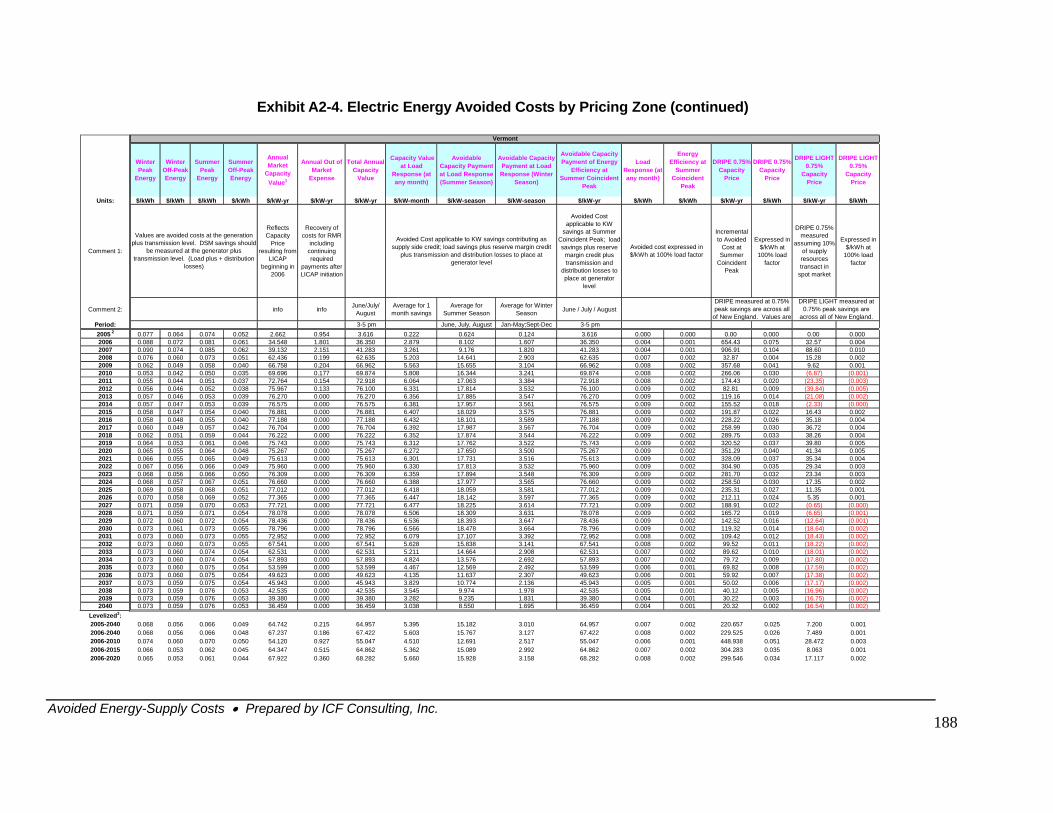
Avoided Energy-Supply Costs • Prepared by ICF Consulting, Inc.
188
Exhibit A2-4. Electric Energy Avoided Costs by Pricing Zone (continued)
Winter Peak
Energy
Winter Off-Peak Energy
Summer Peak
Energy
Summer Off-Peak Energy
Annual Market
Capacity Value1
Annual Out of Market
Expense
Total Annual Capacity
Value
Capacity Value at Load
Response (at any month)
Avoidable Capacity Payment at Load Response (Summer Season)
Avoidable Capacity Payment at Load Response (Winter
Season)
Avoidable Capacity Payment of Energy
Efficiency at Summer Coincident
Peak
Load Response (at any month)
Energy Efficiency at
Summer Coincident
Peak
DRIPE 0.75% Capacity
Price
DRIPE 0.75% Capacity
Price
DRIPE LIGHT 0.75%
Capacity Price
DRIPE LIGHT 0.75%
Capacity Price
Units: $/kWh $/kWh $/kWh $/kWh $/kW-yr $/kW-yr $/kW-yr $/kW-month $/kW-season $/kW-season $/kW-yr $/kWh $/kWh $/kW-yr $/kWh $/kW-yr $/kWh
omment 1:
Reflects Capacity
Price resulting from
LICAP beginning in
2006
Recovery of costs for RMR
including continuing required
payments after LICAP initiation
Avoided Cost applicable to KW
savings at Summer Coincident Peak; load savings plus reserve
margin credit plus transmission and
distribution losses to place at generator
level
Incremental to Avoided
Cost at Summer
Coincident Peak
Expressed in $/kWh at
100% load factor
DRIPE 0.75% measured
assuming 10% of supply resources transact in
spot market
Expressed in $/kWh at
100% load factor
omment 2: info info June/July/ August
Average for 1 month savings
Average for Summer Season
Average for Winter Season June / July / August
Period: 3-5 pm June, July, August Jan-May;Sept-Dec 3-5 pm2005 2 0.077 0.064 0.074 0.052 2.662 0.954 3.616 0.222 0.624 0.124 3.616 0.000 0.000 0.00 0.000 0.00 0.0002006 0.088 0.072 0.081 0.061 34.548 1.801 36.350 2.879 8.102 1.607 36.350 0.004 0.001 654.43 0.075 32.57 0.0042007 0.090 0.074 0.085 0.062 39.132 2.151 41.283 3.261 9.176 1.820 41.283 0.004 0.001 906.91 0.104 88.60 0.0102008 0.076 0.060 0.073 0.051 62.436 0.199 62.635 5.203 14.641 2.903 62.635 0.007 0.002 32.87 0.004 15.28 0.0022009 0.062 0.049 0.058 0.040 66.758 0.204 66.962 5.563 15.655 3.104 66.962 0.008 0.002 357.68 0.041 9.62 0.0012010 0.053 0.042 0.050 0.035 69.696 0.177 69.874 5.808 16.344 3.241 69.874 0.008 0.002 266.06 0.030 (6.87) (0
C
C
2011 0.055 0.044 0.051 0.037 72.764 0.154 72.918 6.064 17.063 3.384 72.918 0.008 0.002 174.43 0.020 (23.35) (2012 0.056 0.046 0.052 0.038 75.967 0.133 76.100 6.331 17.814 3.532 76.100 0.009 0.002 82.81 0.009 (39.84) (2013 0.057 0.046 0.053 0.039 76.270 0.000 76.270 6.356 17.885 3.547 76.270 0.009 0.002 119.16 0.014 (21.08) (2014 0.057 0.047 0.053 0.039 76.575 0.000 76.575 6.381 17.957 3.561 76.575 0.009 0.002 155.52 0.018 (2.33) (2015 0.058 0.047 0.054 0.040 76.881 0.000 76.881 6.407 18.029 3.575 76.881 0.009 0.002 191.87 0.022 16.43 02016 0.058 0.048 0.055 0.040 77.188 0.000 77.188 6.432 18.101 3.589 77.188 0.009 0.002 228.22 0.026 35.18 0.0042017 0.060 0.049 0.057 0.042 76.704 0.000 76.704 6.392 17.987 3.567 76.704 0.009 0.002 258.99 0.030 36.72 0.0042018 0.062 0.051 0.059 0.044 76.222 0.000 76.222 6.352 17.874 3.544 76.222 0.009 0.002 289.75 0.033 38.26 0.0042019 0.064 0.053 0.061 0.046 75.743 0.000 75.743 6.312 17.762 3.522 75.743 0.009 0.002 320.52 0.037 39.80 0.0052020 0.065 0.055 0.064 0.048 75.267 0.000 75.267 6.272 17.650 3.500 75.267 0.009 0.002 351.29 0.040 41.34 0.0052021 0.066 0.055 0.065 0.049 75.613 0.000 75.613 6.301 17.731 3.516 75.613 0.009 0.002 328.09 0.037 35.34 0.0042022 0.067 0.056 0.066 0.049 75.960 0.000 75.960 6.330 17.813 3.532 75.960 0.009 0.002 304.90 0.035 29.34 0.0032023 0.068 0.056 0.066 0.050 76.309 0.000 76.309 6.359 17.894 3.548 76.309 0.009 0.002 281.70 0.032 23.34 0.0032024 0.068 0.057 0.067 0.051 76.660 0.000 76.660 6.388 17.977 3.565 76.660 0.009 0.002 258.50 0.030 17.35 0.0022025 0.069 0.058 0.068 0.051 77.012 0.000 77.012 6.418 18.059 3.581 77.012 0.009 0.002 235.31 0.027 11.35 0.0012026 0.070 0.058 0.069 0.052 77.365 0.000 77.365 6.447 18.142 3.597 77.365 0.009 0.002 212.11 0.024 5.35 0.0012027 0.071 0.059 0.070 0.053 77.721 0.000 77.721 6.477 18.225 3.614 77.721 0.009 0.002 188.91 0.022 (0.65) (0.000)2028 0.071 0.059 0.071 0.054 78.078 0.000 78.078 6.506 18.309 3.631 78.078 0.009 0.002 165.72 0.019 (6.65) (02029 0.072 0.060 0.072 0.054 78.436 0.000 78.436 6.536 18.393 3.647 78.436 0.009 0.002 142.52 0.016 (12.64) (02030 0.073 0.061 0.073 0.055 78.796 0.000 78.796 6.566 18.478 3.664 78.796 0.009 0.002 119.32 0.014 (18.64) (2031 0.073 0.060 0.073 0.055 72.952 0.000 72.952 6.079 17.107 3.392 72.952 0.008 0.002 109.42 0.012 (18.43) (2032 0.073 0.060 0.073 0.055 67.541 0.000 67.541 5.628 15.838 3.141 67.541 0.008 0.002 99.52 0.011 (18.22) (2033 0.073 0.060 0.074 0.054 62.531 0.000 62.531 5.211 14.664 2.908 62.531 0.007 0.002 89.62 0.010 (18.01) (2034 0.073 0.060 0.074 0.054 57.893 0.000 57.893 4.824 13.576 2.692 57.893 0.007 0.002 79.72 0.009 (17.80) (2035 0.073 0.060 0.075 0.054 53.599 0.000 53.599 4.467 12.569 2.492 53.599 0.006 0.001 69.82 0.008 (17.59) (2036 0.073 0.060 0.075 0.054 49.623 0.000 49.623 4.135 11.637 2.307 49.623 0.006 0.001 59.92 0.007 (17.38) (2037 0.073 0.059 0.075 0.054 45.943 0.000 45.943 3.829 10.774 2.136 45.943 0.005 0.001 50.02 0.006 (17.17) (2038 0.073 0.059 0.076 0.053 42.535 0.000 42.535 3.545 9.974 1.978 42.535 0.005 0.001 40.12 0.005 (16.96) (2039 0.073 0.059 0.076 0.053 39.380 0.000 39.380 3.282 9.235 1.831 39.380 0.004 0.001 30.22 0.003 (16.75) (2040 0.073 0.059 0.076 0.053 36.459 0.000 36.459 3.038 8.550 1.695 36.459 0.004 0.001 20.32 0.002 (16.54) (
Levelized3: 2005-2040 0.068 0.056 0.066 0.049 64.742 0.215 64.957 5.395 15.182 3.010 64.957 0.007 0.002 220.657 0.025 7.2002006-2040 0.068 0.056 0.066 0.048 67.237 0.186 67.422 5.603 15.767 3.127 67.422 0.008 0.002 229.525 0.026 7.489 0.0012006-2010 0.074 0.060 0.070 0.050 54.120 0.927 55.047 4.510 12.691 2.517 55.047 0.006 0.001 448.938 0.051 28.472 0.0032006-2015 0.066 0.053 0.062 0.045 64.347 0.515 64.862 5.362 15.089 2.992 64.862 0.007 0.002 304.283 0.035 8.063 0.0012006-2020 0.065 0.053 0.061 0.044 67.922 0.360 68.282 5.660 15.928 3.158 68.282 0.008 0.002 299.546 0.034 17.117 0.002
.001)0.003)0.005)0.002)0.000).002
.001)
.001)0.002)0.002)0.002)0.002)0.002)0.002)0.002)0.002)0.002)0.002)0.002)
0.001
Vermont
Avoided cost expressed in $/kWh at 100% load factor
Values are avoided costs at the generation plus transmission level. DSM savings should
be measured at the generator plus transmission level. (Load plus + distribution
losses)
Avoided Cost applicable to KW savings contributing as supply side credit; load savings plus reserve margin credit
plus transmission and distribution losses to place at generator level
DRIPE measured at 0.75% peak savings are across all
of New England. Values are
DRIPE LIGHT measured at 0.75% peak savings are
across all of New England.
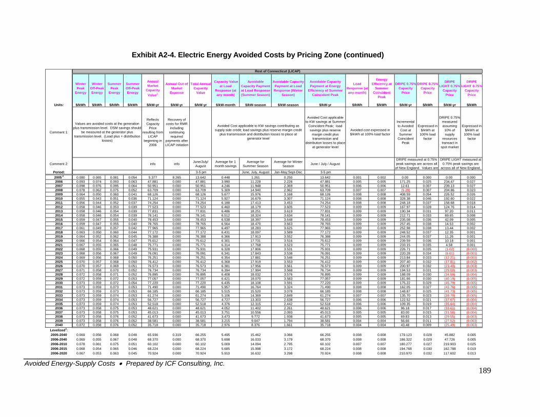
Avoided Energy-Supply Costs • Prepared by ICF Consulting, Inc.
189
Exhibit A2-4. Electric Energy Avoided Costs by Pricing Zone (continued)
Winter Peak
Energy
Winter Off-Peak Energy
Summer Peak
Energy
Summer Off-Peak Energy
Annual Market
Capacity Value1
Annual Out of Market
Expense
Total Annual Capacity
Value
Capacity Value at Load
Response (at any month)
Avoidable Capacity Payment at Load Response (Summer Season)
Avoidable Capacity Payment at Load Response (Winter
Season)
Avoidable Capacity Payment at Energy
Efficiency of Summer Coincident Peak
Load Response (at any month)
Energy Efficiency at
Summer Coincident
Peak
DRIPE 0.75% Capacity
Price
DRIPE 0.75% Capacity
Price
DRIPELIGHT 0.75%
CapacitPrice
Units: $/kWh $/kWh $/kWh $/kWh $/kW-
y
DRIPE LIGHT 0.75%
Capacity Price
yr $/kW-yr $/kW-yr $/kW-month $/kW-season $/kW-season $/kW-yr $/kWh $/kWh $/kW-yr $/kWh $/kW-yr $/kWh
ed
s
ket
Expressed in $/kWh at
100% load factor
0.0000.0270.027
04.86 0.0232009 0.064 0.050 0.060 0.041 68.126 0.000 68.126 5.677 15.976 3.168 68.126 0.008 0.008 408.59 0.054 26.52 0.0262010 0.055 0.043 0.051 0.036 71.124 0.000 71.124 5.927 16.679 3.307 71.124 0.008 0.008 328.38 0.046 92.60 0.0222011 0.056 0.044 0.052 0.037 74.254 0.000 74.254 6.188 17.413 3.453 74.254 0.008 0.008 248.18 0.037 58.68 0.0182012 0.058 0.046 0.053 0.039 77.523 0.000 77.523 6.460 18.179 3.605 77.523 0.009 0.009 167.97 0.028 24.76 0.0142013 0.058 0.046 0.054 0.039 77.831 0.000 77.831 6.486 18.251 3.619 77.831 0.009 0.009 190.34 0.031 97.20 0.0112014 0.058 0.046 0.054 0.039 78.141 0.000 78.141 6.512 18.324 3.634 78.141 0.009 0.009 212.71 0.033 69.65 0.0082015 0.059 0.047 0.055 0.040 78.453 0.000 78.453 6.538 18.397 3.648 78.453 0.009 0.009 235.08 0.036 42.09 0.0052016 0.059 0.047 0.055 0.040 78.765 0.000 78.765 6.564 18.470 3.663 78.765 0.009 0.009 257.45 0.038 14.53 0.0022017 0.061 0.049 0.057 0.042 77.965 0.000 77.965 6.497 18.283 3.625 77.965 0.009 0.009 252.98 0.038 13.44 0.0022018 0.063 0.050 0.060 0.044 77.172 0.000 77.172 6.431 18.097 3.589 77.172 0.009 0.009 248.52 0.037 12.35 0.0012019 0.064 0.052 0.062 0.045 76.388 0.000 76.388 6.366 17.913 3.552 76.388 0.009 0.009 244.05 0.037 11.26 0.0012020 0.066 0.054 0.064 0.047 75.612 0.000 75.612 6.301 17.731 3.516 75.612 0.009 0.009 239.59 0.036 10.18 0.0012021 0.067 0.055 0.065 0.048 75.771 0.000 75.771 6.314 17.768 3.523 75.771 0.009 0.009 233.15 0.035 4.58 0.0012022 0.068 0.055 0.066 0.049 75.931 0.000 75.931 6.328 17.806 3.531 75.931 0.009 0.009 226.71 0.035 (1.02) (0.000)2023 0.068 0.056 0.067 0.049 76.091 0.000 76.091 6.341 17.843 3.538 76.091 0.009 0.009 220.28 0.034 (6.61) (0.001)2024 0.069 0.056 0.068 0.050 76.251 0.000 76.251 6.354 17.881 3.546 76.251 0.009 0.009 213.84 0.033 12.21) (0.001)2025 0.070 0.057 0.068 0.050 76.412 0.000 76.412 6.368 17.919 3.553 76.412 0.009 0.009 207.40 0.032 17.81) (0.002)2026 0.070 0.057 0.069 0.051 76.573 0.000 76.573 6.381 17.956 3.561 76.573 0.009 0.009 200.97 0.032 23.40) (0.003)2027 0.071 0.058 0.070 0.052 76.734 0.000 76.734 6.394 17.994 3.568 76.734 0.009 0.009 194.53 0.031 29.00) (0.003)2028 0.072 0.058 0.071 0.052 76.895 0.000 76.895 6.408 18.032 3.576 76.895 0.009 0.009 188.09 0.030 34.59) (0.004)2029 0.072 0.059 0.072 0.053 77.057 0.000 77.057 6.421 18.070 3.583 77.057 0.009 0.009 181.66 0.030 40.19) (0.005)2030 0.073 0.059 0.072 0.054 77.220 0.000 77.220 6.435 18.108 3.591 77.220 0.009 0.009 175.22 0.029 45.79) (0.005)2031 0.073 0.059 0.073 0.053 71.490 0.000 71.490 5.957 16.764 3.324 71.490 0.008 0.008 162.05 0.027 43.76) (0.005)2032 0.073 0.059 0.073 0.053 66.185 0.000 66.185 5.515 15.520 3.078 66.185 0.008 0.008 148.87 0.025 41.73) (0.005)2033 0.073 0.059 0.074 0.053 61.274 0.000 61.274 5.106 14.369 2.849 61.274 0.007 0.007 135.70 0.023 39.70) (0.005)2034 0.073 0.059 0.074 0.053 56.727 0.000 56.727 4.727 13.303 2.638 56.727 0.006 0.006 122.52 0.021 37.67) (0.004)2035 0.073 0.059 0.074 0.053 52.518 0.000 52.518 4.376 12.315 2.442 52.518 0.006 0.006 109.35 0.019 35.64) (0.004)2036 0.073 0.058 0.075 0.053 48.621 0.000 48.621 4.052 11.402 2.261 48.621 0.006 0.006 96.18 0.017 33.61) (0.004)2037 0.073 0.058 0.075 0.053 45.013 0.000 45.013 3.751 10.556 2.093 45.013 0.005 0.005 83.00 0.015 31.58) (0.004)2038 0.073 0.058 0.076 0.052 41.673 0.000 41.673 3.473 9.772 1.938 41.673 0.005 0.005 69.83 0.013 (29.55) (0.003)2039 0.073 0.058 0.076 0.052 38.581 0.000 38.581 3.215 9.047 1.794 38.581 0.004 0.004 56.66 0.011 (27.52) (0.003)2040 0.072 0.058 0.076 0.052 35.718 0.000 35.718 2.976 8.376 1.661 35.718 0.004 0.004 43.48 0.009 (25.49) (0.003)
Levelized3: 2005-2040 0.069 0.056 0.068 0.048 65.936 0.319 66.255 5.495 15.462 3.066 66.255 0.008 0.008 179.123 0.028 45.882 0.0052006-2040 0.069 0.055 0.067 0.048 68.370 0.000 68.370 5.698 16.033 3.179 68.370 0.008 0.008 186.322 0.029 47.726 0.0052006-2010 0.078 0.061 0.075 0.051 60.102 0.000 60.102 5.009 14.094 2.795 60.102 0.007 0.007 180.277 0.027 219.903 0.0252006-2015 0.068 0.054 0.065 0.046 68.224 0.000 68.224 5.685 15.998 3.172 68.224 0.008 0.008 194.768 0.030 162.788 0.0192006-2020 0.067 0.053 0.063 0.045 70.924 0.000 70.924 5.910 16.632 3.298 70.924 0.008 0.008 210.970 0.032 117.602 0.013
Rest of Connecticut (LICAP)
DRIPE LIGHT measured at 0.75% peak savings are
across all of New England.
Values are avoided costs at the generation plus transmission level. DSM savings should
be measured at the generator plus transmission level. (Load plus + distribution
losses)
Avoided Cost applicable to KW savings contributing as supply side credit; load savings plus reserve margin credit
plus transmission and distribution losses to place at generator level
Avoided cost expressed in $/kWh at 100% load factor
DRIPE measured at 0.75% peak savings are across all
of New England. Values are
Comment 1:
Reflects Capacity
Price resulting from
LICAP beginning in
2006
Recovery of costs for RMR
including continuing required
payments after LICAP initiation
Avoided Cost applicable to KW savings at Summer
Coincident Peak; load savings plus reserve
margin credit plus transmission and
distribution losses to place at generator level
Incremental to Avoided
Cost at Summer
Coincident Peak
Expressed in $/kWh at
100% load factor
DRIPE 0.75% measurassuming
10% ofsupply
resourcetransact in
spot mar
Comment 2: info info June/July/ August
Average for 1 month savings
Average for Summer Season
Average for Winter Season June / July / August
Period: 3-5 pm June, July, August Jan-May;Sept-Dec 3-5 pm2005 2 0.080 0.065 0.081 0.054 5.377 8.265 13.642 0.448 1.261 0.250 13.642 0.001 0.002 0.00 0.000 0.002006 0.093 0.074 0.093 0.063 47.881 0.000 47.881 3.990 11.228 2.226 47.881 0.005 0.005 171.25 0.025 234.472007 0.098 0.076 0.095 0.064 50.951 0.000 50.951 4.246 11.948 2.369 50.951 0.006 0.006 12.61 0.007 239.132008 0.078 0.062 0.075 0.052 63.709 0.000 63.709 5.309 14.940 2.962 63.709 0.007 0.007 (5.29) 0.007 2
2111
((((((((((((((
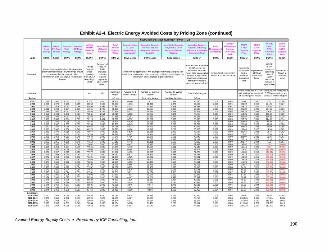
Avoided Energy-Supply Costs • Prepared by ICF Consulting, Inc.
190
Exhibit A2-4. Electric Energy Avoided Costs by Pricing Zone (continued)
Winter Peak
Energy
Winter Off-Peak Energy
Summer Peak
Energy
Summer Off-Peak Energy
Annual Market
Capacity Value1
Annual Out of Market Expense
Total Annual
Capacity Value
Capacity Value at Load
Response (at any month)
Avoidable Capacity Payment at Load
Response (Summer Season)
Avoidable Capacity Payment at Load Response (Winter
Season)
Avoidable Capacity Payment of Energy
Efficiency at Summer Coincident Peak
Load Response (at any month)
Energy Efficiency at
Summer Coincident
Peak
DRIPE 0.75%
Capacity Price
DRIPE 0.75%
Capacity Price
DRIPE LIGHT 0.75%
Capacity Price
DRIPE LIGHT 0.75%
Capacity Price
Units: $/kWh $/kWh $/kWh $/kWh $/kW-yr $/kW-yr $/kW-yr $/kW-month $/kW-season $/kW-season $/kW-yr $/kWh $/kWh $/kW-yr $/kWh $/kW-yr $/kWh
Comment 1:
Reflects Capacity
Price resulting
from LICAP beginning in
2006
Recovery of costs for
RMR including
continuing required
payments after LICAP
initiation
Avoided Cost applicable to KW savings at
Summer Coincident Peak; load savings plus
reserve margin credit plus transmission and distribution losses to
place at generator level
Incremental to Avoided
Cost at Summer
Coincident Peak
Expressed in $/kWh at
100% load factor
DRIPE 0.75%
measured assuming
10% of supply
resources transact in
spot market
Expressed in $/kWh at
100% load factor
Comment 2: info info June/July/ August
Average for 1 month savings
Average for Summer Season
Average for Winter Season June / July / August
Period: 3-5 pm June, July, August Jan-May;Sept-Dec 3-5 pm2005 2 0.082 0.067 0.083 0.055 8.154 18.702 26.856 0.680 1.912 0.379 26.856 0.001 0.003 0.00 0.000 0.00 0.0002006 0.095 0.076 0.096 0.065 48.863 7.638 56.500 4.072 11.458 2.272 56.500 0.006 0.006 436.02 0.050 234.47 0.0272007 0.100 0.078 0.097 0.066 51.995 5.896 57.891 4.333 12.193 2.418 57.891 0.006 0.007 239.13 0.027 239.13 0.0272008 0.081 0.064 0.077 0.053 66.341 1.795 68.136 5.528 15.557 3.085 68.136 0.008 0.008 225.80 0.026 204.86 0.0232009 0.066 0.051 0.061 0.042 70.934 1.742 72.676 5.911 16.634 3.298 72.676 0.008 0.008 493.24 0.056 226.52 0.0262010 0.056 0.044 0.052 0.037 73.561 1.654 75.215 6.130 17.250 3.421 75.215 0.008 0.009 418.06
42.88
.21) 001)7.81) 002)3.40) 003)9.00) 003)4.59) 004)0.19) 005)5.79) 005)3.76) 005)1.73) 005)9.70) 005)7.67) 004)5.64) 004)3.61) 004)1.58) 004)9.55) 003)7.52) 003)5.49) 003)
5.88 0057.726 005
0.048 192.60 0.0222011 0.058 0.045 0.053 0.038 76.285 1.570 77.855 6.357 17.889 3.547 77.855 0.009 0.009 3 0.039 158.68 0.0182012 0.059 0.046 0.054 0.039 79.110 1.491 80.600 6.592 18.551 3.679 80.600 0.009 0.009 267.70 0.031 124.76 0.0142013 0.059 0.046 0.055 0.039 79.424 0.000 79.424 6.619 18.625 3.693 79.424 0.009 0.009 259.64 0.030 97.20 0.0112014 0.060 0.047 0.055 0.039 79.739 0.000 79.739 6.645 18.699 3.708 79.739 0.009 0.009 251.59 0.029 69.65 0.0082015 0.060 0.047 0.056 0.040 80.055 0.000 80.055 6.671 18.773 3.723 80.055 0.009 0.009 243.54 0.028 42.09 0.0052016 0.060 0.047 0.056 0.040 80.373 0.000 80.373 6.698 18.847 3.737 80.373 0.009 0.009 235.49 0.027 14.53 0.0022017 0.062 0.049 0.058 0.041 79.557 0.000 79.557 6.630 18.656 3.699 79.557 0.009 0.009 231.65 0.026 13.44 0.0022018 0.063 0.051 0.060 0.043 78.749 0.000 78.749 6.562 18.467 3.662 78.749 0.009 0.009 227.81 0.026 12.35 0.0012019 0.065 0.052 0.063 0.045 77.949 0.000 77.949 6.496 18.279 3.625 77.949 0.009 0.009 223.97 0.026 11.26 0.0012020 0.067 0.054 0.065 0.047 77.157 0.000 77.157 6.430 18.093 3.588 77.157 0.009 0.009 220.13 0.025 10.18 0.0012021 0.068 0.055 0.066 0.048 77.319 0.000 77.319 6.443 18.131 3.595 77.319 0.009 0.009 208.47 0.024 4.58 0.0012022 0.068 0.056 0.067 0.049 77.482 0.000 77.482 6.457 18.170 3.603 77.482 0.009 0.009 196.82 0.022 (1.02) (0.000)2023 0.069 0.056 0.067 0.049 77.645 0.000 77.645 6.470 18.208 3.611 77.645 0.009 0.009 185.16 0.021 (6.61) (0.001)2024 0.069 0.057 0.068 0.050 77.809 0.000 77.809 6.484 18.246 3.618 77.809 0.009 0.009 173.51 0.020 (12 (0.2025 0.070 0.057 0.069 0.050 77.972 0.000 77.972 6.498 18.285 3.626 77.972 0.009 0.009 161.85 0.018 (1 (0.2026 0.071 0.058 0.070 0.051 78.137 0.000 78.137 6.511 18.323 3.633 78.137 0.009 0.009 150.20 0.017 (2 (0.2027 0.071 0.058 0.070 0.052 78.301 0.000 78.301 6.525 18.362 3.641 78.301 0.009 0.009 138.54 0.016 (2 (0.2028 0.072 0.059 0.071 0.052 78.466 0.000 78.466 6.539 18.400 3.649 78.466 0.009 0.009 126.89 0.014 (3 (0.2029 0.073 0.060 0.072 0.053 78.631 0.000 78.631 6.553 18.439 3.656 78.631 0.009 0.009 115.23 0.013 (4 (0.2030 0.073 0.060 0.073 0.054 78.796 0.000 78.796 6.566 18.478 3.664 78.796 0.009 0.009 103.57 0.012 (4 (0.2031 0.073 0.060 0.073 0.054 72.952 0.000 72.952 6.079 17.107 3.392 72.952 0.008 0.008 94.54 0.011 (4 (0.2032 0.073 0.060 0.074 0.054 67.541 0.000 67.541 5.628 15.838 3.141 67.541 0.008 0.008 85.51 0.010 (4 (0.2033 0.073 0.060 0.074 0.053 62.531 0.000 62.531 5.211 14.664 2.908 62.531 0.007 0.007 76.48 0.009 (3 (0.2034 0.073 0.060 0.075 0.053 57.893 0.000 57.893 4.824 13.576 2.692 57.893 0.007 0.007 67.45 0.008 (3 (0.2035 0.074 0.060 0.075 0.053 53.599 0.000 53.599 4.467 12.569 2.492 53.599 0.006 0.006 58.42 0.007 (3 (0.2036 0.074 0.059 0.076 0.053 49.623 0.000 49.623 4.135 11.637 2.307 49.623 0.006 0.006 49.39 0.006 (3 (0.2037 0.074 0.059 0.076 0.053 45.943 0.000 45.943 3.829 10.774 2.136 45.943 0.005 0.005 40.36 0.005 (3 (0.2038 0.074 0.059 0.077 0.053 42.535 0.000 42.535 3.545 9.974 1.978 42.535 0.005 0.005 31.33 0.004 (2 (0.2039 0.074 0.059 0.077 0.053 39.380 0.000 39.380 3.282 9.235 1.831 39.380 0.004 0.004 22.30 0.003 (2 (0.2040 0.074 0.059 0.078 0.053 36.459 0.000 36.459 3.038 8.550 1.695 36.459 0.004 0.004 13.27 0.002 (2 (0.
Levelized3: 2005-2040 0.070 0.056 0.069 0.049 67.539 1.520 69.059 5.628 15.838 3.141 69.059 0.008 0.008 196.91 0.022 4 0.2006-2040 0.070 0.056 0.068 0.049 69.926 0.829 70.755 5.827 16.398 3.252 70.755 0.008 0.008 204.825 0.023 4 0.2006-2010 0.080 0.063 0.077 0.053 62.064 3.810 65.874 5.172 14.554 2.886 65.874 0.007 0.008 361.593 0.041 219.903 0.0252006-2015 0.070 0.055 0.067 0.046 70.054 2.300 72.354 5.838 16.428 3.258 72.354 0.008 0.008 319.966 0.037 162.788 0.0192006-2020 0.068 0.054 0.065 0.045 72.679 1.609 74.288 6.057 17.043 3.380 74.288 0.008 0.008 292.324 0.033 117.602 0.013
DRIPE LIGHT measured at 0.75% peak savings are
across all of New England.
DRIPE measured at 0.75% peak savings are across all
of New England. Values
Southwest Connecticut (NOR RTEP + SWCT RTEP)
Avoided cost expressed in $/kWh at 100% load factor
Values are avoided costs at the generation plus transmission level. DSM savings should
be measured at the generator plus transmission level. (Load plus + distribution
losses)
Avoided Cost applicable to KW savings contributing as supply side credit; load savings plus reserve margin credit plus transmission and
distribution losses to place at generator level
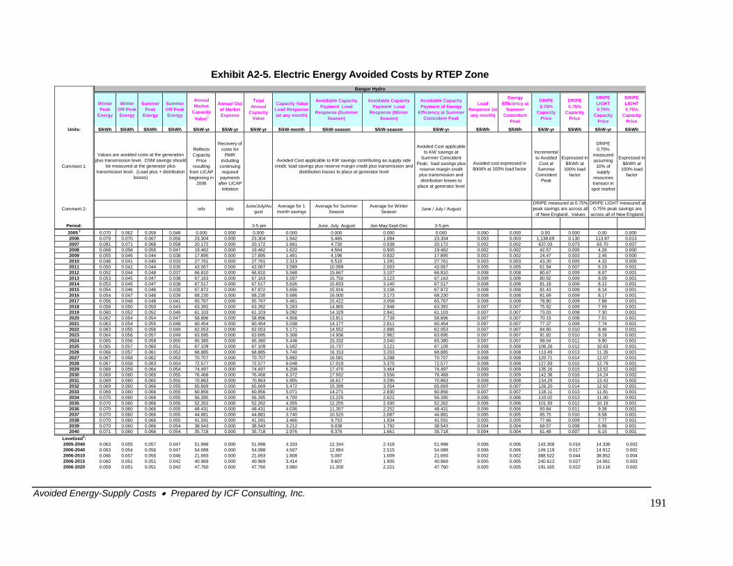
Avoided Energy-Supply Costs • Prepared by ICF Consulting, Inc.
191
Exhibit A2-5. Electric Energy Avoided Costs by RTEP Zone
Winter Peak
Energy
Winter Off-Peak Energy
Summer Peak
Energy
Summer Off-Peak Energy
Annual Market
Capacity Value1
Annual Out of Market Expense
Total Annual
Capacity Value
Capacity Value Load Response (at any month)
Avoidable Capacity Payment Load
Response (Summer Season)
Avoidable Capacity Payment Load
Response (Winter Season)
Avoidable Capacity Payment of Energy
Efficiency at Summer Coincident Peak
Load Response (at any month)
Energy Efficiency at
Summer Coincident
Peak
DRIPE 0.75%
Capacity Price
DRIPE 0.75%
Capacity Price
DRIPE LIGHT 0.75%
Capacity Price
DRIPE LIGHT 0.75%
Capacity Price
Units: $/kWh $/kWh $/kWh $/kWh $/kW-yr $/kW-yr $/kW-yr $/kW-month $/kW-season $/kW-season $/kW-yr $/kWh $/kWh $/kW-yr $/kWh $/kW-yr $/kWh
Comment 1:
Reflects Capacity
Price resulting
from LICAP beginning in
2006
Recovery of costs for
RMR including
continuing required
payments after LICAP
initiation
Avoided Cost applicable to KW savings at
Summer Coincident Peak; load savings plus
reserve margin credit plus transmission and distribution losses to
place at generator level
Incremental to Avoided
Cost at Summer
Coincident Peak
Expressed in $/kWh at
100% load factor
DRIPE 0.75%
measured assuming
10% of supply
resources transact in
spot market
Expressed in $/kWh at
100% load factor
Comment 2: info info June/July/August
Average for 1 month savings
Average for Summer Season
Average for Winter Season June / July / August
Period: 3-5 pm June, July, August Jan-May;Sept-Dec 3-5 pm2005 2 0.070 0.062 0.059 0.048 0.000 0.000 0.000 0.000 0.000 0.000 0.000 0.000 0.000 0.00 0.000 0.00 0.0002006 0.079 0.070 0.067 0.056 23.304 0.000 23.304 1.942 5.465 1.084 23.304 0.003 0.003 1,138.69 0.130 113.87 0.0132007 0.081 0.071 0.068 0.058 20.172 0.000 20.172 1.681 4.730 0.938 20.172 0.002 0.002 637.03 0.073 63.70 0.0072008 0.068 0.058 0.055 0.047 19.462 0.000 19.462 1.622 4.564 0.905 19.462 0.002 0.002 42.57 0.005 4.26 0.0002009 0.055 0.046 0.044 0.038 17.895 0.000 17.895 1.491 4.196 0.832 17.895 0.002 0.002 24.47 0.003 2.45 0.0002010 0.048 0.041 0.040 0.033 27.761 0.000 27.761 2.313 6.510 1.291 27.761 0.003 0.003 43.20 0.005 4.32 0.0002011 0.050 0.042 0.044 0.035 43.067 0.000 43.067 3.589 10.099 2.003 43.067 0.005 0.005 61.94 0.007 6.19 0.0012012 0.052 0.044 0.048 0.037 66.810 0.000 66.810 5.568 15.667 3.107 66.810 0.008 0.008 80.67 0.009 8.07 0.0012013 0.053 0.045 0.047 0.038 67.163 0.000 67.163 5.597 15.750 3.123 67.163 0.008 0.008 80.92 0.009 8.09 0.0012014 0.053 0.045 0.047 0.038 67.517 0.000 67.517 5.626 15.833 3.140 67.517 0.008 0.008 81.18 0.009 8.12 0.0012015 0.054 0.046 0.046 0.039 67.872 0.000 67.872 5.656 15.916 3.156 67.872 0.008 0.008 81.43 0.009 8.14 0.0012016 0.054 0.047 0.046 0.039 68.230 0.000 68.230 5.686 16.000 3.173 68.230 0.008 0.008 81.69 0.009 8.17 0.0012017 0.056 0.048 0.048 0.041 65.767 0.000 65.767 5.481 15.422 3.058 65.767 0.008 0.008 78.80 0.009 7.88 0.0012018 0.058 0.050 0.050 0.043 63.392 0.000 63.392 5.283 14.865 2.948 63.392 0.007 0.007 75.92 0.009 7.59 0.0012019 0.060 0.052 0.052 0.045 61.103 0.000 61.103 5.092 14.329 2.841 61.103 0.007 0.007 73.03 0.008 7.30 0.0012020 0.062 0.054 0.054 0.047 58.896 0.000 58.896 4.908 13.811 2.739 58.896 0.007 0.007 70.15 0.008 7.01 0.0012021 0.063 0.054 0.055 0.048 60.454 0.000 60.454 5.038 14.177 2.811 60.454 0.007 0.007 77.37 0.009 7.74 0.001
8.46 0.0019.18 0.0019.90 0.001
10.63 0.00111.35 0.00112.07 0.00112.79 0.00113.52 0.00214.24 0.00213.43 0.00212.62 0.00111.81 0.00111.00 0.00110.19 0.0019.38 0.0018.58 0.0017.77 0.0016.96 0.0016.15 0.001
2022 0.063 0.055 0.056 0.049 62.053 0.000 62.053 5.171 14.552 2.885 62.053 0.007 0.007 84.60 0.0102023 0.064 0.056 0.057 0.049 63.695 0.000 63.695 5.308 14.936 2.962 63.695 0.007 0.007 91.82 0.0102024 0.065 0.056 0.059 0.050 65.380 0.000 65.380 5.448 15.332 3.040 65.380 0.007 0.007 99.04 0.0112025 0.065 0.057 0.060 0.051 67.109 0.000 67.109 5.592 15.737 3.121 67.109 0.008 0.008 106.26 0.0122026 0.066 0.057 0.061 0.052 68.885 0.000 68.885 5.740 16.153 3.203 68.885 0.008 0.008 113.49 0.0132027 0.067 0.058 0.062 0.053 70.707 0.000 70.707 5.892 16.581 3.288 70.707 0.008 0.008 120.71 0.0142028 0.067 0.058 0.063 0.054 72.577 0.000 72.577 6.048 17.019 3.375 72.577 0.008 0.008 127.93 0.0152029 0.068 0.059 0.064 0.054 74.497 0.000 74.497 6.208 17.470 3.464 74.497 0.009 0.009 135.16 0.0152030 0.069 0.060 0.065 0.055 76.468 0.000 76.468 6.372 17.932 3.556 76.468 0.009 0.009 142.38 0.0162031 0.069 0.060 0.065 0.055 70.863 0.000 70.863 5.905 16.617 3.295 70.863 0.008 0.008 134.29 0.0152032 0.069 0.060 0.066 0.055 65.669 0.000 65.669 5.472 15.399 3.054 65.669 0.007 0.007 126.20 0.0142033 0.069 0.060 0.066 0.055 60.856 0.000 60.856 5.071 14.271 2.830 60.856 0.007 0.007 118.11 0.0132034 0.070 0.060 0.066 0.055 56.395 0.000 56.395 4.700 13.225 2.622 56.395 0.006 0.006 110.02 0.0132035 0.070 0.060 0.066 0.055 52.262 0.000 52.262 4.355 12.255 2.430 52.262 0.006 0.006 101.93 0.0122036 0.070 0.060 0.066 0.055 48.431 0.000 48.431 4.036 11.357 2.252 48.431 0.006 0.006 93.84 0.0112037 0.070 0.060 0.066 0.055 44.881 0.000 44.881 3.740 10.525 2.087 44.881 0.005 0.005 85.75 0.0102038 0.070 0.060 0.066 0.055 41.591 0.000 41.591 3.466 9.753 1.934 41.591 0.005 0.005 77.66 0.0092039 0.070 0.060 0.066 0.054 38.543 0.000 38.543 3.212 9.038 1.792 38.543 0.004 0.004 69.57 0.0082040 0.071 0.060 0.066 0.054 35.718 0.000 35.718 2.976 8.376 1.661 35.718 0.004 0.004 61.48 0.007
Levelized3: 2005-2040 0.063 0.055 0.057 0.047 51.998 0.000 51.998 4.333 12.194 2.418 51.998 0.006 0.006 143.358 0.016 14.336 0.0022006-2040 0.063 0.054 0.056 0.047 54.088 0.000 54.088 4.507 12.684 2.515 54.088 0.006 0.006 149.119 0.017 14.912 0.0022006-2010 0.066 0.057 0.055 0.046 21.693 0.000 21.693 1.808 5.087 1.009 21.693 0.002 0.002 388.522 0.044 38.852 0.0042006-2015 0.060 0.051 0.051 0.042 40.969 0.000 40.969 3.414 9.607 1.905 40.969 0.005 0.005 240.613 0.027 24.061 0.0032006-2020 0.059 0.051 0.051 0.042 47.760 0.000 47.760 3.980 11.200 2.221 47.760 0.005 0.005 191.165 0.022 19.116 0.002
DRIPE measured at 0.75% peak savings are across all
of New England. Values
DRIPE LIGHT measured at 0.75% peak savings are
across all of New England.
Values are avoided costs at the generation plus transmission level. DSM savings should
be measured at the generator plus transmission level. (Load plus + distribution
losses)
Avoided cost expressed in $/kWh at 100% load factor
Bangor Hydro
Avoided Cost applicable to KW savings contributing as supply side credit; load savings plus reserve margin credit plus transmission and
distribution losses to place at generator level
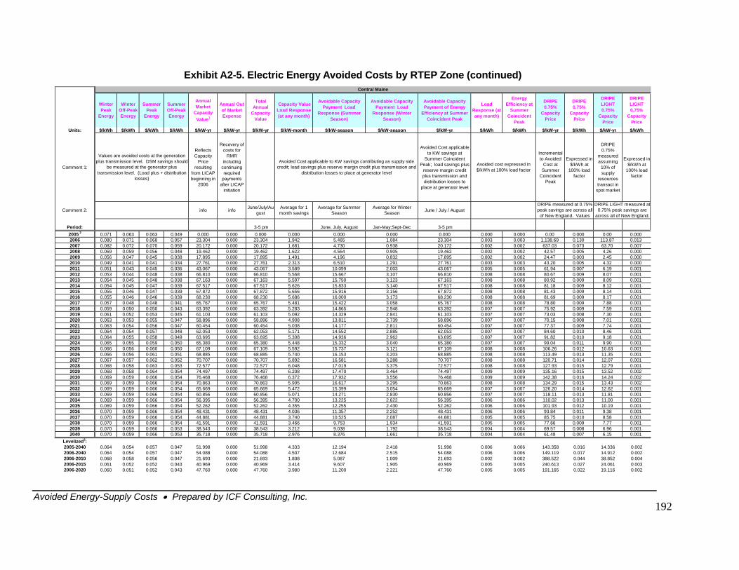
Avoided Energy-Supply Costs • Prepared by ICF Consulting, Inc.
192
Exhibit A2-5. Electric Energy Avoided Costs by RTEP Zone (continued)
Winter Peak
Energy
Winter Off-Peak Energy
Summer Peak
Energy
Summer Off-Peak Energy
Annual Market
Capacity Value1
Annual Out of Market Expense
Total Annual
Capacity Value
Capacity Value Load Response (at any month)
Avoidable Capacity Payment Load
Response (Summer Season)
Avoidable Capacity Payment Load
Response (Winter Season)
Avoidable Capacity Payment of Energy
Efficiency at Summer Coincident Peak
Load Response (at any month)
Energy Efficiency at
Summer Coincident
Peak
DRIPE 0.75%
Capacity Price
DRIPE 0.75%
Capacity Price
DRIPE LIGHT 0.75%
Capacity Price
DRIPE LIGHT 0.75%
Capacity Price
Units: $/kWh $/kWh $/kWh $/kWh $/kW-yr $/kW-yr $/kW-yr $/kW-month $/kW-season $/kW-season $/kW-yr $/kWh $/kWh $/kW-yr $/kWh $/kW-yr $/kWh
Comment 1:
Reflects Capacity
Price resulting
from LICAP beginning in
2006
Recovery of costs for
RMR including
continuing required
payments after LICAP
initiation
Avoided Cost applicable to KW savings at
Summer Coincident Peak; load savings plus
reserve margin credit plus transmission and distribution losses to
place at generator level
Incremental to Avoided
Cost at Summer
Coincident Peak
Expressed in $/kWh at
100% load factor
DRIPE 0.75%
measured assuming
10% of supply
resources transact in
spot market
Expressed in $/kWh at
100% load factor
Comment 2: info info June/July/August
Average for 1 month savings
Average for Summer Season
Average for Winter Season June / July / August
Period: 3-5 pm June, July, August Jan-May;Sept-Dec 3-5 pm2005 2 0.071 0.063 0.063 0.049 0.000 0.000 0.000 0.000 0.000 0.000 0.000 0.000 0.000 0.00 0.000 0.00 0.0002006 0.080 0.071 0.068 0.057 23.304 0.000 23.304 1.942 5.465 1.084 23.304 0.003 0.003 1,138.69 0.130 113.87 0.0132007 0.082 0.072 0.070 0.059 20.172 0.000 20.172 1.681 4.730 0.938 20.172 0.002 0.002 637.03 0.073 63.70 0.0072008 0.069 0.059 0.056 0.048 19.462 0.000 19.462 1.622 4.564 0.905 19.462 0.002 0.002 42.57 0.005 4.26 0.0002009 0.056 0.047 0.045 0.038 17.895 0.000 17.895 1.491 4.196 0.832 17.895 0.002 0.002 24.47 0.003 2.45 0.0002010 0.049 0.041 0.041 0.034 27.761 0.000 27.761 2.313 6.510 1.291 27.761 0.003 0.003 43.20 0.005 4.32 0.0002011 0.051 0.043 0.045 0.036 43.067 0.000 43.067 3.589 10.099 2.003 43.067 0.005 0.005 61.94 0.007 6.19 0.0012012 0.053 0.044 0.048 0.038 66.810 0.000 66.810 5.568 15.667 3.107 66.810 0.008 0.008 80.67 0.009 8.07 0.0012013 0.054 0.045 0.048 0.038 67.163 0.000 67.163 5.597 15.750 3.123 67.163 0.008 0.008 80.92 0.009 8.09 0.0012014 0.054 0.045 0.047 0.039 67.517 0.000 67.517 5.626 15.833 3.140 67.517 0.008 0.008 81.18 0.009 8.12 0.0012015 0.055 0.046 0.047 0.039 67.872 0.000 67.872 5.656 15.916 3.156 67.872 0.008 0.008 81.43 0.009 8.14 0.0012016 0.055 0.046 0.046 0.039 68.230 0.000 68.230 5.686 16.000 3.173 68.230 0.008 0.008 81.69 0.009 8.17 0.0012017 0.057 0.048 0.048 0.041 65.767 0.000 65.767 5.481 15.422 3.058 65.767 0.008 0.008 78.80 0.009 7.88 0.0012018 0.059 0.050 0.050 0.043 63.392 0.000 63.392 5.283 14.865 2.948 63.392 0.007 0.007 75.92 0.009 7.59 0.0012019 0.061 0.052 0.053 0.045 61.103 0.000 61.103 5.092 14.329 2.841 61.103 0.007 0.007 73.03 0.008 7.30 0.0012020 0.063 0.053 0.055 0.047 58.896 0.000 58.896 4.908 13.811 2.739 58.896 0.007 0.007 70.15 0.008 7.01 0.0012021 0.063 0.054 0.056 0.047 60.454 0.000 60.454 5.038 14.177 2.811 60.454 0.007 0.007 77.37 0.009 7.74 0.0012022 0.064 0.054 0.057 0.048 62.053 0.000 62.053 5.171 14.552 2.885 62.053 0.007 0.007 84.60 0.010 8.46 0.0012023 0.064 0.055 0.058 0.049 63.695 0.000 63.695 5.308 14.936 2.962 63.695 0.007 0.007 91.82 0.010 9.18 0.0012024 0.065 0.055 0.059 0.050 65.380 0.000 65.380 5.448 15.332 3.040 65.380 0.007 0.007 99.04 0.011 9.90 0.0012025 0.066 0.056 0.060 0.050 67.109 0.000 67.109 5.592 15.737 3.121 67.109 0.008 0.008 106.26 0.012 10.63 0.0012026 0.066 0.056 0.061 0.051 68.885 0.000 68.885 5.740 16.153 3.203 68.885 0.008 0.008 113.49 0.013 11.35 0.0012027 0.067 0.057 0.062 0.052 70.707 0.000 70.707 5.892 16.581 3.288 70.707 0.008 0.008 120.71 0.014 12.07 0.0012028 0.068 0.058 0.063 0.053 72.577 0.000 72.577 6.048 17.019 3.375 72.577 0.008 0.008 127.93 0.015 12.79 0.0012029 0.068 0.058 0.064 0.054 74.497 0.000 74.497 6.208 17.470 3.464 74.497 0.009 0.009 135.16 0.015 13.52 0.0022030 0.069 0.059 0.066 0.054 76.468 0.000 76.468 6.372 17.932 3.556 76.468 0.009 0.009 142.38 0.016 14.24 0.0022031 0.069 0.059 0.066 0.054 70.863 0.000 70.863 5.905 16.617 3.295 70.863 0.008 0.008 134.29 0.015 13.43 0.0022032 0.069 0.059 0.066 0.054 65.669 0.000 65.669 5.472 15.399 3.054 65.669 0.007 0.007 126.20 0.014 12.62 0.0012033 0.069 0.059 0.066 0.054 60.856 0.000 60.856 5.071 14.271 2.830 60.856 0.007 0.007 118.11 0.013 11.81 0.0012034 0.069 0.059 0.066 0.054 56.395 0.000 56.395 4.700 13.225 2.622 56.395 0.006 0.006 110.02 0.013 11.00 0.0012035 0.069 0.059 0.066 0.054 52.262 0.000 52.262 4.355 12.255 2.430 52.262 0.006 0.006 101.93 0.012 10.19 0.0012036 0.070 0.059 0.066 0.054 48.431 0.000 48.431 4.036 11.357 2.252 48.431 0.006 0.006 93.84 0.011 9.38 0.0012037 0.070 0.059 0.066 0.054 44.881 0.000 44.881 3.740 10.525 2.087 44.881 0.005 0.005 85.75 0.010 8.58 0.0012038 0.070 0.059 0.066 0.054 41.591 0.000 41.591 3.466 9.753 1.934 41.591 0.005 0.005 77.66 0.009 7.77 0.0012039 0.070 0.059 0.066 0.053 38.543 0.000 38.543 3.212 9.038 1.792 38.543 0.004 0.004 69.57 0.008 6.96 0.0012040 0.070 0.059 0.066 0.053 35.718 0.000 35.718 2.976 8.376 1.661 35.718 0.004 0.004 61.48 0.007 6.15 0.001
Levelized3: 2005-2040 0.064 0.054 0.057 0.047 51.998 0.000 51.998 4.333 12.194 2.418 51.998 0.006 0.006 143.358 0.016 14.336 0.0022006-2040 0.064 0.054 0.057 0.047 54.088 0.000 54.088 4.507 12.684 2.515 54.088 0.006 0.006 149.119 0.017 14.912 0.0022006-2010 0.068 0.058 0.056 0.047 21.693 0.000 21.693 1.808 5.087 1.009 21.693 0.002 0.002 388.522 0.044 38.852 0.0042006-2015 0.061 0.052 0.052 0.043 40.969 0.000 40.969 3.414 9.607 1.905 40.969 0.005 0.005 240.613 0.027 24.061 0.0032006-2020 0.060 0.051 0.052 0.043 47.760 0.000 47.760 3.980 11.200 2.221 47.760 0.005 0.005 191.165 0.022 19.116 0.002
Central Maine
Values are avoided costs at the generation plus transmission level. DSM savings should
be measured at the generator plus transmission level. (Load plus + distribution
losses)
DRIPE measured at 0.75% peak savings are across all
of New England. Values
DRIPE LIGHT measured at 0.75% peak savings are
across all of New England.
Avoided cost expressed in $/kWh at 100% load factor
Avoided Cost applicable to KW savings contributing as supply side credit; load savings plus reserve margin credit plus transmission and
distribution losses to place at generator level
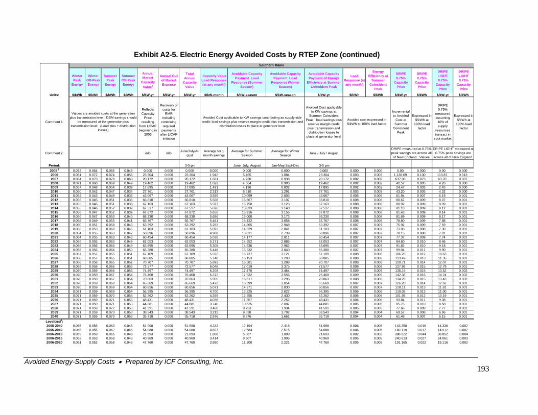
Exhibit A2-5. Electric Energy Avoided Costs by RTEP Zone (continued)
Winter Peak
Energy
Winter Off-Peak Energy
Summer Peak
Energy
Summer Off-Peak Energy
Annual Market
Capacity Value1
Annual Out of Market Expense
Total Annual
Capacity Value
Capacity Value Load Response (at any month)
Avoidable Capacity Payment Load
Response (Summer Season)
Avoidable Capacity Payment Load
Response (Winter Season)
Avoidable Capacity Payment of Energy
Efficiency at Summer Coincident Peak
Load Response (at any month)
Energy Efficiency at
Summer Coincident
Peak
DRIPE 0.75%
Capacity Price
DRIPE 0.75%
Capacity Price
DRIPE LIGHT 0.75%
Capacity Price
DRIPE LIGHT 0.75%
Capacity Price
Units: $/kWh $/kWh $/kWh $/kWh $/kW-yr $/kW-yr $/kW-yr $/kW-month $/kW-season $/kW-season $/kW-yr $/kWh $/kWh $/kW-yr $/kWh $/kW-yr $/kWh
Comment 1:
Reflects Capacity
Price resulting
from LICAP beginning in
2006
Recovery of costs for
RMR including
continuing required
payments after LICAP
initiation
Avoided Cost applicable to KW savings at
Summer Coincident Peak; load savings plus
reserve margin credit plus transmission and distribution losses to
place at generator level
Incremental to Avoided
Cost at Summer
Coincident Peak
Expressed in $/kWh at
100% load factor
DRIPE 0.75%
measured assuming
10% of supply
resources transact in
spot market
Expressed in $/kWh at
100% load factor
Comment 2: info info June/July/August
Average for 1 month savings
Average for Summer Season
Average for Winter Season June / July / August
Period: 3-5 pm June, July, August Jan-May;Sept-Dec 3-5 pm2005 2 0.072 0.064 0.066 0.049 0.000 0.000 0.000 0.000 0.000 0.000 0.000 0.000 0.000 0.00 0.000 0.00 0.0002006 0.081 0.072 0.074 0.058 23.304 0.000 23.304 1.942 5.465 1.084 23.304 0.003 0.003 1,138.69 0.130 113.87 0.0132007 0.084 0.073 0.078 0.060 20.172 0.000 20.172 1.681 4.730 0.938 20.172 0.002 0.002 637.03 0.073 63.70 0.0072008 0.071 0.060 0.069 0.049 19.462 0.000 19.462 1.622 4.564 0.905 19.462 0.002 0.002 42.57 0.005 4.26 0.0002009 0.057 0.048 0.054 0.039 17.895 0.000 17.895 1.491 4.196 0.832 17.895 0.002 0.002 24.47 0.003 2.45 0.0002010 0.050 0.042 0.047 0.034 27.761 0.000 27.761 2.313 6.510 1.291 27.761 0.003 0.003 43.20 0.005 4.32 0.0002011 0.052 0.043 0.049 0.036 43.067 0.000 43.067 3.589 10.099 2.003 43.067 0.005 0.005 61.94 0.007 6.19 0.0012012 0.055 0.045 0.051 0.038 66.810 0.000 66.810 5.568 15.667 3.107 66.810 0.008 0.008 80.67 0.009 8.07 0.0012013 0.055 0.046 0.051 0.038 67.163 0.000 67.163 5.597 15.750 3.123 67.163 0.008 0.008 80.92 0.009 8.09 0.0012014 0.055 0.046 0.052 0.039 67.517 0.000 67.517 5.626 15.833 3.140 67.517 0.008 0.008 81.18 0.009 8.12 0.0012015 0.056 0.047 0.052 0.039 67.872 0.000 67.872 5.656 15.916 3.156 67.872 0.008 0.008 81.43 0.009 8.14 0.0012016 0.056 0.047 0.053 0.040 68.230 0.000 68.230 5.686 16.000 3.173 68.230 0.008 0.008 81.69 0.009 8.17 0.0012017 0.058 0.049 0.055 0.041 65.767 0.000 65.767 5.481 15.422 3.058 65.767 0.008 0.008 78.80 0.009 7.88 0.0012018 0.060 0.051 0.058 0.043 63.392 0.000 63.392 5.283 14.865 2.948 63.392 0.007 0.007 75.92 0.009 7.59 0.0012019 0.062 0.053 0.060 0.045 61.103 0.000 61.103 5.092 14.329 2.841 61.103 0.007 0.007 73.03 0.008 7.30 0.0012020 0.064 0.055 0.063 0.047 58.896 0.000 58.896 4.908 13.811 2.739 58.896 0.007 0.007 70.15 0.008 7.01 0.0012021 0.064 0.055 0.063 0.048 60.454 0.000 60.454 5.038 14.177 2.811 60.454 0.007 0.007 77.37 0.009 7.74 0.0012022 0.065 0.055 0.063 0.049 62.053 0.000 62.053 5.171 14.552 2.885 62.053 0.007 0.007 84.60 0.010 8.46 0.0012023 0.066 0.056 0.064 0.049 63.695 0.000 63.695 5.308 14.936 2.962 63.695 0.007 0.007 91.82 0.010 9.18 0.0012024 0.066 0.056 0.064 0.050 65.380 0.000 65.380 5.448 15.332 3.040 65.380 0.007 0.007 99.04 0.011 9.90 0.0012025 0.067 0.057 0.065 0.051 67.109 0.000 67.109 5.592 15.737 3.121 67.109 0.008 0.008 106.26 0.012 10.63 0.0012026 0.068 0.057 0.065 0.051 68.885 0.000 68.885 5.740 16.153 3.203 68.885 0.008 0.008 113.49 0.013 11.35 0.0012027 0.068 0.058 0.065 0.052 70.707 0.000 70.707 5.892 16.581 3.288 70.707 0.008 0.008 120.71 0.014 12.07 0.0012028 0.069 0.058 0.066 0.053 72.577 0.000 72.577 6.048 17.019 3.375 72.577 0.008 0.008 127.93 0.015 12.79 0.0012029 0.070 0.059 0.066 0.053 74.497 0.000 74.497 6.208 17.470 3.464 74.497 0.009 0.009 135.16 0.015 13.52 0.0022030 0.070 0.059 0.067 0.054 76.468 0.000 76.468 6.372 17.932 3.556 76.468 0.009 0.009 142.38 0.016 14.24 0.0022031 0.070 0.059 0.067 0.054 70.863 0.000 70.863 5.905 16.617 3.295 70.863 0.008 0.008 134.29 0.015 13.43 0.0022032 0.070 0.059 0.068 0.054 65.669 0.000 65.669 5.472 15.399 3.054 65.669 0.007 0.007 126.20 0.014 12.62 0.0012033 0.070 0.059 0.069 0.054 60.856 0.000 60.856 5.071 14.271 2.830 60.856 0.007 0.007 118.11 0.013 11.81 0.0012034 0.071 0.059 0.069 0.054 56.395 0.000 56.395 4.700 13.225 2.622 56.395 0.006 0.006 110.02 0.013 11.00 0.0012035 0.071 0.059 0.070 0.054 52.262 0.000 52.262 4.355 12.255 2.430 52.262 0.006 0.006 101.93 0.012 10.19 0.0012036 0.071 0.059 0.071 0.053 48.431 0.000 48.431 4.036 11.357 2.252 48.431 0.006 0.006 93.84 0.011 9.38 0.0012037 0.071 0.059 0.071 0.053 44.881 0.000 44.881 3.740 10.525 2.087 44.881 0.005 0.005 85.75 0.010 8.58 0.0012038 0.071 0.059 0.072 0.053 41.591 0.000 41.591 3.466 9.753 1.934 41.591 0.005 0.005 77.66 0.009 7.77 0.0012039 0.071 0.059 0.073 0.053 38.543 0.000 38.543 3.212 9.038 1.792 38.543 0.004 0.004 69.57 0.008 6.96 0.0012040 0.071 0.059 0.073 0.053 35.718 0.000 35.718 2.976 8.376 1.661 35.718 0.004 0.004 61.48 0.007 6.15 0.001
Levelized3: 2005-2040 0.065 0.055 0.063 0.048 51.998 0.000 51.998 4.333 12.194 2.418 51.998 0.006 0.006 143.358 0.016 14.336 0.0022006-2040 0.065 0.055 0.062 0.048 54.088 0.000 54.088 4.507 12.684 2.515 54.088 0.006 0.006 149.119 0.017 14.912 0.0022006-2010 0.069 0.059 0.065 0.048 21.693 0.000 21.693 1.808 5.087 1.009 21.693 0.002 0.002 388.522 0.044 38.852 0.0042006-2015 0.062 0.053 0.058 0.043 40.969 0.000 40.969 3.414 9.607 1.905 40.969 0.005 0.005 240.613 0.027 24.061 0.0032006-2020 0.061 0.052 0.058 0.043 47.760 0.000 47.760 3.980 11.200 2.221 47.760 0.005 0.005 191.165 0.022 19.116 0.002
Southern Maine
DRIPE LIGHT measured at 0.75% peak savings are
across all of New England.
Values are avoided costs at the generation plus transmission level. DSM savings should
be measured at the generator plus transmission level. (Load plus + distribution
losses)
Avoided cost expressed in $/kWh at 100% load factor
DRIPE measured at 0.75% peak savings are across all
of New England. Values
Avoided Cost applicable to KW savings contributing as supply side credit; load savings plus reserve margin credit plus transmission and
distribution losses to place at generator level
Avoided Energy-Supply Costs • Prepared by ICF Consulting, Inc.
193
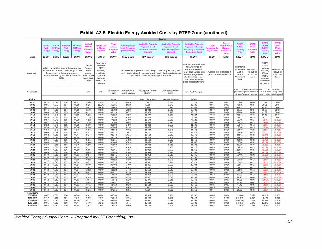
Avoided Energy-Supply Costs • Prepared by ICF Consulting, Inc.
194
Exhibit A2-5. Electric Energy Avoided Costs by RTEP Zone (continued)
Winter Peak
Energy
Winter Off-Peak Energy
Summer Peak
Energy
Summer Off-Peak Energy
Annual Market
Capacity Value1
Annual Out of Market Expense
Total Annual
Capacity Value
Capacity Value Load Response (at any month)
Avoidable Capacity Payment Load
Response (Summer Season)
Avoidable Capacity Payment Load
Response (Winter Season)
Avoidable Capacity Payment of Energy
Efficiency at Summer Coincident Peak
Load Response (at any month)
Energy Efficiency at
Summer Coincident
Peak
DRIPE 0.75%
Capacity Price
DRIPE 0.75%
Capacity Price
DRIPE LIGHT 0.75%
Capacity Price
DRIPE LIGHT 0.75%
Capacity Price
Units: $/kWh $/kWh $/kWh $/kWh $/kW-yr $/kW-yr $/kW-yr $/kW-month $/kW-season $/kW-season $/kW-yr $/kWh $/kWh $/kW-yr $/kWh $/kW-yr $/kWh
Comment 1:
Reflects Capacity
Price resulting
from LICAP beginning in
2006
Recovery of costs for
RMR including
continuing required
payments after LICAP
initiation
Avoided Cost applicable to KW savings at
Summer Coincident Peak; load savings plus
reserve margin credit plus transmission and distribution losses to
place at generator level
Incremental to Avoided
Cost at Summer
Coincident Peak
Expressed in $/kWh at
100% load factor
DRIPE 0.75%
measured assuming
10% of supply
resources transact in
spot market
Expressed in $/kWh at
100% load factor
Comment 2: info info June/July/August
Average for 1 month savings
Average for Summer Season
Average for Winter Season June / July / August
Period: 3-5 pm June, July, August Jan-May;Sept-Dec 3-5 pm2005 2 0.074 0.064 0.069 0.051 5.387 4.835 10.222 0.449 1.263 0.251 10.222 0.001 0.001 0.00 0.000 0.00 0.0002006 0.085 0.072 0.077 0.059 35.258 11.077 46.335 2.938 8.268 1.640 46.335 0.004 0.005 739.33 0.084 38.81 0.0042007 0.087 0.074 0.081 0.062 39.936 9.630 49.566 3.328 9.365 1.857 49.566 0.005 0.006 978.41 0.112 54.89 0.0062008 0.074 0.060 0.072 0.050 63.709 0.000 63.709 5.309 14.940 2.962 63.709 0.007 0.007 35.09 0.004 15.58 0.0022009 0.060 0.049 0.056 0.040 68.126 0.000 68.126 5.677 15.976 3.168 68.126 0.008 0.008 436.08 0.050 41.82 0.0052010 0.052 0.042 0.049 0.035 71.124 0.000 71.124 5.927 16.679 3.307 71.124 0.008 0.008 332.41 0.038 23.40 0.0032011 0.055 0.044 0.051 0.037 74.254 0.000 74.254 6.188 17.413 3.453 74.254 0.008 0.008 228.74 0.026 4.97 0.0012012 0.057 0.046 0.052 0.038 77.523 0.000 77.523 6.460 18.179 3.605 77.523 0.009 0.009 125.06 0.014 (13.45) (0.002)2013 0.057 0.046 0.053 0.039 79.296 0.000 79.296 6.608 18.595 3.687 79.296 0.009 0.009 142.39 0.016 (13.40) (0.002)2014 0.058 0.046 0.054 0.039 81.109 0.000 81.109 6.759 19.020 3.772 81.109 0.009 0.009 159.72 0.018 (13.35) (0.002)2015 0.058 0.047 0.054 0.040 82.965 0.000 82.965 6.914 19.455 3.858 82.965 0.009 0.009 177.04 0.020 (13.30) (0.002)2016 0.059 0.047 0.055 0.040 84.862 0.000 84.862 7.072 19.900 3.946 84.862 0.010 0.010 194.37 0.022 (13.25) (0.002)2017 0.060 0.049 0.057 0.042 84.012 0.000 84.012 7.001 19.701 3.907 84.012 0.010 0.010 218.99 0.025 (10.11) (0.001)2018 0.062 0.051 0.059 0.044 83.170 0.000 83.170 6.931 19.503 3.867 83.170 0.009 0.009 243.61 0.028 (6.97) (0.001)2019 0.064 0.053 0.061 0.045 82.336 0.000 82.336 6.861 19.308 3.829 82.336 0.009 0.009 268.23 0.031 (3.84) (0.000)2020 0.066 0.055 0.064 0.047 81.511 0.000 81.511 6.793 19.114 3.790 81.511 0.009 0.009 292.85 0.033 (0.70) (0.000)2021 0.066 0.055 0.065 0.048 81.400 0.000 81.400 6.783 19.088 3.785 81.400 0.009 0.009 277.03 0.032 (2.19) (0.000)2022 0.067 0.056 0.065 0.049 81.288 0.000 81.288 6.774 19.062 3.780 81.288 0.009 0.009 261.21 0.030 (3.68) (0.000)2023 0.068 0.056 0.066 0.049 81.177 0.000 81.177 6.765 19.036 3.775 81.177 0.009 0.009 245.39 0.028 (5.17) (0.001)2024 0.068 0.057 0.067 0.050 81.066 0.000 81.066 6.756 19.010 3.770 81.066 0.009 0.009 229.57 0.026 (6.66) (0.001)2025 0.069 0.057 0.068 0.051 80.956 0.000 80.956 6.746 18.984 3.764 80.956 0.009 0.009 213.75 0.024 (8.16) (0.001)2026 0.070 0.058 0.069 0.051 80.845 0.000 80.845 6.737 18.958 3.759 80.845 0.009 0.009 197.93 0.023 (9.65) (0.001)2027 0.070 0.059 0.069 0.052 80.735 0.000 80.735 6.728 18.932 3.754 80.735 0.009 0.009 182.10 0.021 (11.14) (0.001)2028 0.071 0.059 0.070 0.053 80.624 0.000 80.624 6.719 18.906 3.749 80.624 0.009 0.009 166.28 0.019 (12.63) (0.001)2029 0.072 0.060 0.071 0.054 80.514 0.000 80.514 6.710 18.881 3.744 80.514 0.009 0.009 150.46 0.017 (14.13) (0.002)2030 0.072 0.060 0.072 0.054 80.404 0.000 80.404 6.700 18.855 3.739 80.404 0.009 0.009 134.64 0.015 (15.62) (0.002)2031 0.072 0.060 0.072 0.054 74.442 0.000 74.442 6.203 17.457 3.462 74.442 0.008 0.008 123.74 0.014 (15.42) (0.002)2032 0.072 0.060 0.073 0.054 68.922 0.000 68.922 5.743 16.162 3.205 68.922 0.008 0.008 112.84 0.013 (15.22) (0.002)2033 0.072 0.060 0.073 0.054 63.811 0.000 63.811 5.318 14.964 2.967 63.811 0.007 0.007 101.95 0.012 (15.02) (0.002)2034 0.072 0.060 0.074 0.054 59.079 0.000 59.079 4.923 13.854 2.747 59.079 0.007 0.007 91.05 0.010 (14.82) (0.002)2035 0.072 0.059 0.074 0.053 54.698 0.000 54.698 4.558 12.827 2.543 54.698 0.006 0.006 80.15 0.009 (14.62) (0.002)2036 0.072 0.059 0.074 0.053 50.642 0.000 50.642 4.220 11.876 2.355 50.642 0.006 0.006 69.25 0.008 (14.42) (0.002)2037 0.072 0.059 0.075 0.053 46.887 0.000 46.887 3.907 10.995 2.180 46.887 0.005 0.005 58.36 0.007 (14.22) (0.002)2038 0.072 0.059 0.075 0.053 43.410 0.000 43.410 3.618 10.180 2.019 43.410 0.005 0.005 47.46 0.005 (14.02) (0.002)2039 0.072 0.059 0.076 0.053 40.191 0.000 40.191 3.349 9.425 1.869 40.191 0.005 0.005 36.56 0.004 (13.82) (0.002)2040 0.072 0.059 0.076 0.053 37.211 0.000 37.211 3.101 8.726 1.730 37.211 0.004 0.004 25.66 0.003 (13.62) (0.002)
Levelized3: 2005-2040 0.067 0.056 0.065 0.048 67.827 0.964 68.790 5.652 15.905 3.154 68.790 0.008 0.008 225.800 0.026 -1.517 0.0002006-2040 0.067 0.055 0.065 0.048 70.336 0.808 71.144 5.861 16.494 3.271 71.144 0.008 0.008 234.875 0.027 -1.578 0.0002006-2010 0.072 0.060 0.067 0.050 55.228 4.270 59.498 4.602 12.951 2.568 59.498 0.006 0.007 509.740 0.058 35.078 0.0042006-2015 0.065 0.053 0.060 0.044 66.491 2.242 68.733 5.541 15.592 3.092 68.733 0.008 0.008 346.913 0.040 13.879 0.0022006-2020 0.064 0.052 0.060 0.044 71.515 1.568 73.083 5.960 16.770 3.325 73.083 0.008 0.008 315.578 0.036 7.576 0.001
Boston
DRIPE LIGHT measured at 0.75% peak savings are
across all of New England.
Values are avoided costs at the generation plus transmission level. DSM savings should
be measured at the generator plus transmission level. (Load plus + distribution
losses)
Avoided cost expressed in $/kWh at 100% load factor
DRIPE measured at 0.75% peak savings are across all
of New England. Values
Avoided Cost applicable to KW savings contributing as supply side credit; load savings plus reserve margin credit plus transmission and
distribution losses to place at generator level

Exhibit A2-5. Electric Energy Avoided Costs by RTEP Zone (continued)
Winter Peak
Energy
Winter Off-Peak Energy
Summer Peak
Energy
Summer Off-Peak Energy
Annual Market
Capacity Value1
Annual Out of Market Expense
Total Annual
Capacity Value
Capacity Value Load Response (at any month)
Avoidable Capacity Payment Load
Response (Summer Season)
Avoidable Capacity Payment Load
Response (Winter Season)
Avoidable Capacity Payment of Energy
Efficiency at Summer Coincident Peak
Load Response (at any month)
Energy Efficiency at
Summer Coincident
Peak
DRIPE 0.75%
Capacity Price
DRIPE 0.75%
Capacity Price
DRIPE LIGHT 0.75%
Capacity Price
DRIPE LIGHT 0.75%
Capacity Price
Units: $/kWh $/kWh $/kWh $/kWh $/kW-yr $/kW-yr $/kW-yr $/kW-month $/kW-season $/kW-season $/kW-yr $/kWh $/kWh $/kW-yr $/kWh $/kW-yr $/kWh
Comment 1:
Reflects Capacity
Price resulting
from LICAP beginning in
2006
Recovery of costs for
RMR including
continuing required
payments after LICAP
initiation
Avoided Cost applicable to KW savings at
Summer Coincident Peak; load savings plus
reserve margin credit plus transmission and distribution losses to
place at generator level
Incremental to Avoided
Cost at Summer
Coincident Peak
Expressed in $/kWh at
100% load factor
DRIPE 0.75%
measured assuming
10% of supply
resources transact in
spot market
Expressed in $/kWh at
100% load factor
Comment 2: info info June/July/August
Average for 1 month savings
Average for Summer Season
Average for Winter Season June / July / August
Period: 3-5 pm June, July, August Jan-May;Sept-Dec 3-5 pm2005 2 0.074 0.064 0.069 0.051 2.662 0.954 3.616 0.222 0.624 0.124 3.616 0.000 0.000 0.00 0.000 0.00 0.0002006 0.085 0.072 0.077 0.059 34.548 1.801 36.350 2.879 8.102 1.607 36.350 0.004 0.004 654.43 0.075 32.57 0.0042007 0.087 0.074 0.081 0.062 39.132 2.151 41.283 3.261 9.176 1.820 41.283 0.004 0.005 906.91 0.104 88.60 0.0102008 0.074 0.060 0.072 0.050 62.436 0.199 62.635 5.203 14.641 2.903 62.635 0.007 0.007 32.87 0.004 15.28 0.0022009 0.060 0.049 0.056 0.040 66.758 0.204 66.962 5.563 15.655 3.104 66.962 0.008 0.008 357.68 0.041 9.62 0.0012010 0.052 0.042 0.049 0.035 69.696 0.177 69.874 5.808 16.344 3.241 69.874 0.008 0.008 266.06 0.030 (6.87) (0.001)2011 0.055 0.044 0.051 0.037 72.764 0.154 72.918 6.064 17.063 3.384 72.918 0.008 0.008 174.43 0.020 (23.35) (0.003)2012 0.057 0.046 0.052 0.038 75.967 0.133 76.100 6.331 17.814 3.532 76.100 0.009 0.009 82.81 0.009 (39.84) (0.005)
(21.08) (0.002)(2.33) (0.000)16.43 0.00235.18 0.00436.72 0.00438.26 0.00439.80 0.00541.34 0.00535.34 0.00429.34 0.00323.34 0.00317.35 0.00211.35 0.0015.35 0.001(0.65) (0.000)(6.65) (0.001)
(12.64) (0.001)(18.64) (0.002)(18.43) (0.002)(18.22) (0.002)(18.01) (0.002)(17.80) (0.002)(17.59) (0.002)(17.38) (0.002)(17.17) (0.002)(16.96) (0.002)(16.75) (0.002)(16.54) (0.002)
2013 0.057 0.046 0.053 0.039 76.270 0.000 76.270 6.356 17.885 3.547 76.270 0.009 0.009 119.16 0.0142014 0.058 0.046 0.054 0.039 76.575 0.000 76.575 6.381 17.957 3.561 76.575 0.009 0.009 155.52 0.0182015 0.058 0.047 0.054 0.040 76.881 0.000 76.881 6.407 18.029 3.575 76.881 0.009 0.009 191.87 0.0222016 0.059 0.047 0.055 0.040 77.188 0.000 77.188 6.432 18.101 3.589 77.188 0.009 0.009 228.22 0.0262017 0.060 0.049 0.057 0.042 76.704 0.000 76.704 6.392 17.987 3.567 76.704 0.009 0.009 258.99 0.0302018 0.062 0.051 0.059 0.044 76.222 0.000 76.222 6.352 17.874 3.544 76.222 0.009 0.009 289.75 0.0332019 0.064 0.053 0.061 0.045 75.743 0.000 75.743 6.312 17.762 3.522 75.743 0.009 0.009 320.52 0.0372020 0.066 0.055 0.064 0.047 75.267 0.000 75.267 6.272 17.650 3.500 75.267 0.009 0.009 351.29 0.0402021 0.066 0.055 0.065 0.048 75.613 0.000 75.613 6.301 17.731 3.516 75.613 0.009 0.009 328.09 0.0372022 0.067 0.056 0.065 0.049 75.960 0.000 75.960 6.330 17.813 3.532 75.960 0.009 0.009 304.90 0.0352023 0.068 0.056 0.066 0.049 76.309 0.000 76.309 6.359 17.894 3.548 76.309 0.009 0.009 281.70 0.0322024 0.068 0.057 0.067 0.050 76.660 0.000 76.660 6.388 17.977 3.565 76.660 0.009 0.009 258.50 0.0302025 0.069 0.057 0.068 0.051 77.012 0.000 77.012 6.418 18.059 3.581 77.012 0.009 0.009 235.31 0.0272026 0.070 0.058 0.069 0.051 77.365 0.000 77.365 6.447 18.142 3.597 77.365 0.009 0.009 212.11 0.0242027 0.070 0.059 0.069 0.052 77.721 0.000 77.721 6.477 18.225 3.614 77.721 0.009 0.009 188.91 0.0222028 0.071 0.059 0.070 0.053 78.078 0.000 78.078 6.506 18.309 3.631 78.078 0.009 0.009 165.72 0.0192029 0.072 0.060 0.071 0.054 78.436 0.000 78.436 6.536 18.393 3.647 78.436 0.009 0.009 142.52 0.0162030 0.072 0.060 0.072 0.054 78.796 0.000 78.796 6.566 18.478 3.664 78.796 0.009 0.009 119.32 0.0142031 0.072 0.060 0.072 0.054 72.952 0.000 72.952 6.079 17.107 3.392 72.952 0.008 0.008 109.42 0.0122032 0.072 0.060 0.073 0.054 67.541 0.000 67.541 5.628 15.838 3.141 67.541 0.008 0.008 99.52 0.0112033 0.072 0.060 0.073 0.054 62.531 0.000 62.531 5.211 14.664 2.908 62.531 0.007 0.007 89.62 0.0102034 0.072 0.060 0.074 0.054 57.893 0.000 57.893 4.824 13.576 2.692 57.893 0.007 0.007 79.72 0.0092035 0.072 0.059 0.074 0.053 53.599 0.000 53.599 4.467 12.569 2.492 53.599 0.006 0.006 69.82 0.0082036 0.072 0.059 0.074 0.053 49.623 0.000 49.623 4.135 11.637 2.307 49.623 0.006 0.006 59.92 0.0072037 0.072 0.059 0.075 0.053 45.943 0.000 45.943 3.829 10.774 2.136 45.943 0.005 0.005 50.02 0.0062038 0.072 0.059 0.075 0.053 42.535 0.000 42.535 3.545 9.974 1.978 42.535 0.005 0.005 40.12 0.0052039 0.072 0.059 0.076 0.053 39.380 0.000 39.380 3.282 9.235 1.831 39.380 0.004 0.004 30.22 0.0032040 0.072 0.059 0.076 0.053 36.459 0.000 36.459 3.038 8.550 1.695 36.459 0.004 0.004 20.32 0.002
Levelized3: 2005-2040 0.067 0.056 0.065 0.048 64.742 0.215 64.957 5.395 15.182 3.010 64.957 0.007 0.007 220.657 0.025 7.200 0.0012006-2040 0.067 0.055 0.065 0.048 67.237 0.186 67.422 5.603 15.767 3.127 67.422 0.008 0.008 229.525 0.026 7.489 0.0012006-2010 0.072 0.060 0.067 0.050 54.120 0.927 55.047 4.510 12.691 2.517 55.047 0.006 0.006 448.938 0.051 28.472 0.0032006-2015 0.065 0.053 0.060 0.044 64.347 0.515 64.862 5.362 15.089 2.992 64.862 0.007 0.007 304.283 0.035 8.063 0.0012006-2020 0.064 0.052 0.060 0.044 67.922 0.360 68.282 5.660 15.928 3.158 68.282 0.008 0.008 299.546 0.034 17.117 0.002
Central Massachusetts
DRIPE LIGHT measured at 0.75% peak savings are
across all of New England.
DRIPE measured at 0.75% peak savings are across all
of New England. Values
Values are avoided costs at the generation plus transmission level. DSM savings should
be measured at the generator plus transmission level. (Load plus + distribution
losses)
Avoided cost expressed in $/kWh at 100% load factor
Avoided Cost applicable to KW savings contributing as supply side credit; load savings plus reserve margin credit plus transmission and
distribution losses to place at generator level
Avoided Energy-Supply Costs • Prepared by ICF Consulting, Inc.
195
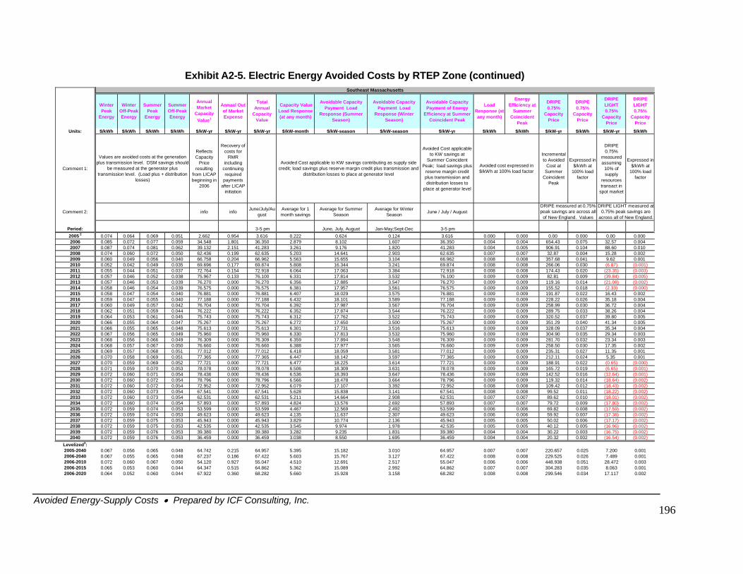
Exhibit A2-5. Electric Energy Avoided Costs by RTEP Zone (continued)
Winter Peak
Energy
Winter Off-Peak Energy
Summer Peak
Energy
Summer Off-Peak Energy
Annual Market
Capacity Value1
Annual Out of Market Expense
Total Annual
Capacity Value
Capacity Value Load Response (at any month)
Avoidable Capacity Payment Load
Response (Summer Season)
Avoidable Capacity Payment Load
Response (Winter Season)
Avoidable Capacity Payment of Energy
Efficiency at Summer Coincident Peak
Load Response (at any month)
Energy Efficiency at
Summer Coincident
Peak
DRIPE 0.75%
Capacity Price
DRIPE 0.75%
Capacity Price
DRIPE LIGHT 0.75%
Capacity Price
DRIPE LIGHT 0.75%
Capacity Price
Units: $/kWh $/kWh $/kWh $/kWh $/kW-yr $/kW-yr $/kW-yr $/kW-month $/kW-season $/kW-season $/kW-yr $/kWh $/kWh $/kW-yr $/kWh $/kW-yr $/kWh
Comment 1:
Reflects Capacity
Price resulting
from LICAP beginning in
2006
Recovery of costs for
RMR including
continuing required
payments after LICAP
initiation
Avoided Cost applicable to KW savings at
Summer Coincident Peak; load savings plus
reserve margin credit plus transmission and distribution losses to
place at generator level
Incremental to Avoided
Cost at Summer
Coincident Peak
Expressed in $/kWh at
100% load factor
DRIPE 0.75%
measured assuming
10% of supply
resources transact in
spot market
Expressed in $/kWh at
100% load factor
Comment 2: info info June/July/August
Average for 1 month savings
Average for Summer Season
Average for Winter Season June / July / August
Period: 3-5 pm June, July, August Jan-May;Sept-Dec 3-5 pm2005 2 0.074 0.064 0.069 0.051 2.662 0.954 3.616 0.222 0.624 0.124 3.616 0.000 0.000 0.00 0.000 0.00 0.0002006 0.085 0.072 0.077 0.059 34.548 1.801 36.350 2.879 8.102 1.607 36.350 0.004 0.004 654.43 0.075 32.57 0.0042007 0.087 0.074 0.081 0.062 39.132 2.151 41.283 3.261 9.176 1.820 41.283 0.004 0.005 906.91 0.104 88.60 0.0102008 0.074 0.060 0.072 0.050 62.436 0.199 62.635 5.203 14.641 2.903 62.635 0.007 0.007 32.87 0.004 15.28 0.0022009 0.060 0.049 0.056 0.040 66.758 0.204 66.962 5.563 15.655 3.104 66.962 0.008 0.008 357.68 0.041 9.62 0.0012010 0.052 0.042 0.049 0.035 69.696 0.177 69.874 5.808 16.344 3.241 69.874 0.008 0.008 266.06 0.030 (6.87) (0.001)
(23.35) (0.003)(39.84) (0.005)(21.08) (0.002)(2.33) (0.000)16.43 0.002
(0.65) (0.000)(6.65) (0.001)
(12.64) (0.001)(18.64) (0.002)(18.43) (0.002)(18.22) (0.002)(18.01) (0.002)(17.80) (0.002)(17.59) (0.002)(17.38) (0.002)(17.17) (0.002)(16.96) (0.002)(16.75) (0.002)(16.54) (0.002)
2011 0.055 0.044 0.051 0.037 72.764 0.154 72.918 6.064 17.063 3.384 72.918 0.008 0.008 174.43 0.0202012 0.057 0.046 0.052 0.038 75.967 0.133 76.100 6.331 17.814 3.532 76.100 0.009 0.009 82.81 0.0092013 0.057 0.046 0.053 0.039 76.270 0.000 76.270 6.356 17.885 3.547 76.270 0.009 0.009 119.16 0.0142014 0.058 0.046 0.054 0.039 76.575 0.000 76.575 6.381 17.957 3.561 76.575 0.009 0.009 155.52 0.0182015 0.058 0.047 0.054 0.040 76.881 0.000 76.881 6.407 18.029 3.575 76.881 0.009 0.009 191.87 0.0222016 0.059 0.047 0.055 0.040 77.188 0.000 77.188 6.432 18.101 3.589 77.188 0.009 0.009 228.22 0.026 35.18 0.0042017 0.060 0.049 0.057 0.042 76.704 0.000 76.704 6.392 17.987 3.567 76.704 0.009 0.009 258.99 0.030 36.72 0.0042018 0.062 0.051 0.059 0.044 76.222 0.000 76.222 6.352 17.874 3.544 76.222 0.009 0.009 289.75 0.033 38.26 0.0042019 0.064 0.053 0.061 0.045 75.743 0.000 75.743 6.312 17.762 3.522 75.743 0.009 0.009 320.52 0.037 39.80 0.0052020 0.066 0.055 0.064 0.047 75.267 0.000 75.267 6.272 17.650 3.500 75.267 0.009 0.009 351.29 0.040 41.34 0.0052021 0.066 0.055 0.065 0.048 75.613 0.000 75.613 6.301 17.731 3.516 75.613 0.009 0.009 328.09 0.037 35.34 0.0042022 0.067 0.056 0.065 0.049 75.960 0.000 75.960 6.330 17.813 3.532 75.960 0.009 0.009 304.90 0.035 29.34 0.0032023 0.068 0.056 0.066 0.049 76.309 0.000 76.309 6.359 17.894 3.548 76.309 0.009 0.009 281.70 0.032 23.34 0.0032024 0.068 0.057 0.067 0.050 76.660 0.000 76.660 6.388 17.977 3.565 76.660 0.009 0.009 258.50 0.030 17.35 0.0022025 0.069 0.057 0.068 0.051 77.012 0.000 77.012 6.418 18.059 3.581 77.012 0.009 0.009 235.31 0.027 11.35 0.0012026 0.070 0.058 0.069 0.051 77.365 0.000 77.365 6.447 18.142 3.597 77.365 0.009 0.009 212.11 0.024 5.35 0.0012027 0.070 0.059 0.069 0.052 77.721 0.000 77.721 6.477 18.225 3.614 77.721 0.009 0.009 188.91 0.0222028 0.071 0.059 0.070 0.053 78.078 0.000 78.078 6.506 18.309 3.631 78.078 0.009 0.009 165.72 0.0192029 0.072 0.060 0.071 0.054 78.436 0.000 78.436 6.536 18.393 3.647 78.436 0.009 0.009 142.52 0.0162030 0.072 0.060 0.072 0.054 78.796 0.000 78.796 6.566 18.478 3.664 78.796 0.009 0.009 119.32 0.0142031 0.072 0.060 0.072 0.054 72.952 0.000 72.952 6.079 17.107 3.392 72.952 0.008 0.008 109.42 0.0122032 0.072 0.060 0.073 0.054 67.541 0.000 67.541 5.628 15.838 3.141 67.541 0.008 0.008 99.52 0.0112033 0.072 0.060 0.073 0.054 62.531 0.000 62.531 5.211 14.664 2.908 62.531 0.007 0.007 89.62 0.0102034 0.072 0.060 0.074 0.054 57.893 0.000 57.893 4.824 13.576 2.692 57.893 0.007 0.007 79.72 0.0092035 0.072 0.059 0.074 0.053 53.599 0.000 53.599 4.467 12.569 2.492 53.599 0.006 0.006 69.82 0.0082036 0.072 0.059 0.074 0.053 49.623 0.000 49.623 4.135 11.637 2.307 49.623 0.006 0.006 59.92 0.0072037 0.072 0.059 0.075 0.053 45.943 0.000 45.943 3.829 10.774 2.136 45.943 0.005 0.005 50.02 0.0062038 0.072 0.059 0.075 0.053 42.535 0.000 42.535 3.545 9.974 1.978 42.535 0.005 0.005 40.12 0.0052039 0.072 0.059 0.076 0.053 39.380 0.000 39.380 3.282 9.235 1.831 39.380 0.004 0.004 30.22 0.0032040 0.072 0.059 0.076 0.053 36.459 0.000 36.459 3.038 8.550 1.695 36.459 0.004 0.004 20.32 0.002
Levelized3: 2005-2040 0.067 0.056 0.065 0.048 64.742 0.215 64.957 5.395 15.182 3.010 64.957 0.007 0.007 220.657 0.025 7.200 0.0012006-2040 0.067 0.055 0.065 0.048 67.237 0.186 67.422 5.603 15.767 3.127 67.422 0.008 0.008 229.525 0.026 7.489 0.0012006-2010 0.072 0.060 0.067 0.050 54.120 0.927 55.047 4.510 12.691 2.517 55.047 0.006 0.006 448.938 0.051 28.472 0.0032006-2015 0.065 0.053 0.060 0.044 64.347 0.515 64.862 5.362 15.089 2.992 64.862 0.007 0.007 304.283 0.035 8.063 0.0012006-2020 0.064 0.052 0.060 0.044 67.922 0.360 68.282 5.660 15.928 3.158 68.282 0.008 0.008 299.546 0.034 17.117 0.002
DRIPE measured at 0.75% peak savings are across all
of New England. Values
DRIPE LIGHT measured at 0.75% peak savings are
across all of New England.
Southeast Massachusetts
Avoided Cost applicable to KW savings contributing as supply side credit; load savings plus reserve margin credit plus transmission and
distribution losses to place at generator level
Values are avoided costs at the generation plus transmission level. DSM savings should
be measured at the generator plus transmission level. (Load plus + distribution
losses)
Avoided cost expressed in $/kWh at 100% load factor
Avoided Energy-Supply Costs • Prepared by ICF Consulting, Inc.
196
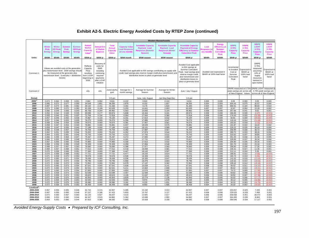
Exhibit A2-5. Electric Energy Avoided Costs by RTEP Zone (continued) Winter
Peak Energy
Winter Off-Peak Energy
Summer Peak
Energy
Summer Off-Peak Energy
Annual Market
Capacity Value1
Annual Out of Market Expense
Total Annual
Capacity Value
Capacity Value Load Response (at any month)
Avoidable Capacity Payment Load
Response (Summer Season)
Avoidable Capacity Payment Load
Response (Winter Season)
Avoidable Capacity Payment of Energy
Efficiency at Summer Coincident Peak
Load Response (at any month)
Energy Efficiency at
Summer Coincident
Peak
DRIPE 0.75%
Capacity Price
DRIPE 0.75%
Capacity Price
DRIPE LIGHT 0.75%
Capacity Price
DRIPE LIGHT 0.75%
Capacity Price
Units: $/kWh $/kWh $/kWh $/kWh $/kW-yr $/kW-yr $/kW-yr $/kW-month $/kW-season $/kW-season $/kW-yr $/kWh $/kWh $/kW-yr $/kWh $/kW-yr $/kWh
Comment 1:
Reflects Capacity
Price resulting
from LICAP beginning in
2006
Recovery of costs for
RMR including
continuing required
payments after LICAP
initiation
Avoided Cost applicable to KW savings at
Summer Coincident Peak; load savings plus
reserve margin credit plus transmission and distribution losses to
place at generator level
Incremental to Avoided
Cost at Summer
Coincident Peak
Expressed in $/kWh at
100% load factor
DRIPE 0.75%
measured assuming
10% of supply
resources transact in
spot market
Expressed i$/kWh at
100% loadfactor
Comment 2: info info June/July/August
Average for 1 month savings
Average for Summer Season
Average for Winter Season June / July / August
Period: 3-5 pm June, July, August Jan-May;Sept-Dec 3-5 pm2005 2 0.074 0.064 0.069 0.051 2.662 0.954 3.616 0.222 0.624 0.124 3.616 0.000 0.000 0.00 0.000 0.00 0.0002006 0.085 0.072 0.077 0.059 34.548 1.801 36.350 2.879 8.102 1.607 36.350 0.004 0.004 654.43 0.075 32.57 0.0042007 0.087 0.074 0.081 0.062 39.132 2.151 41.283 3.261 9.176 1.820 41.283 0.004 0.005 906.91 0.104 88.60 0.0102008 0.074 0.060 0.072 0.050 62.436 0.199 62.635 5.203 14.641 2.903 62.635 0.007 0.007 32.87 0.004 15.28 0.0022009 0.060 0.049 0.056 0.040 66.758 0.204 66.962 5.563 15.655 3.104 66.962 0.008 0.008 357.68 0.041
n
2 12010 0.052 0.042 0.049 0.035 69.696 0.177 69.874 5.808 16.344 3.241 69.874 0.008 0.008 266.06 0.030 7) 01)2011 0.055 0.044 0.051 0.037 72.764 0.154 72.918 6.064 17.063 3.384 72.918 0.008 0.008 174.43 0.020 35) 3)2012 0.057 0.046 0.052 0.038 75.967 0.133 76.100 6.331 17.814 3.532 76.100 0.009 0.009 82.81 0.009 84) 5)2013 0.057 0.046 0.053 0.039 76.270 0.000 76.270 6.356 17.885 3.547 76.270 0.009 0.009 119.16 0.014 08) 2)2014 0.058 0.046 0.054 0.039 76.575 0.000 76.575 6.381 17.957 3.561 76.575 0.009 0.009 155.52 0.018 (2 33) (0. 00)2015 0.058 0.047 0.054 0.040 76.881 0.000 76.881 6.407 18.029 3.575 76.881 0.009 0.009 191.87 0.022 16.43 0.0022016 0.059 0.047 0.055 0.040 77.188 0.000 77.188 6.432 18.101 3.589 77.188 0.009 0.009 228.22 0.026 35.18 0.0042017 0.060 0.049 0.057 0.042 76.704 0.000 76.704 6.392 17.987 3.567 76.704 0.009 0.009 258.99 0.030 36.72 0.0042018 0.062 0.051 0.059 0.044 76.222 0.000 76.222 6.352 17.874 3.544 76.222 0.009 0.009 289.75 0.033 38.26 0.0042019 0.064 0.053 0.061 0.045 75.743 0.000 75.743 6.312 17.762 3.522 75.743 0.009 0.009 320.52 0.037 39.80 0.0052020 0.066 0.055 0.064 0.047 75.267 0.000 75.267 6.272 17.650 3.500 75.267 0.009 0.009 351.29 0.040 41.34 0.0052021 0.066 0.055 0.065 0.048 75.613 0.000 75.613 6.301 17.731 3.516 75.613 0.009 0.009 328.09 0.037 35.34 0.0042022 0.067 0.056 0.065 0.049 75.960 0.000 75.960 6.330 17.813 3.532 75.960 0.009 0.009 304.90 0.035 29.34 0.0032023 0.068 0.056 0.066 0.049 76.309 0.000 76.309 6.359 17.894 3.548 76.309 0.009 0.009 281.70 0.032 23.34 0.0032024 0.068 0.057 0.067 0.050 76.660 0.000 76.660 6.388 17.977 3.565 76.660 0.009 0.009 258.50 0.030 17.35 0.0022025 0.069 0.057 0.068 0.051 77.012 0.000 77.012 6.418 18.059 3.581 77.012 0.009 0.009 235.31 0.027 11.35 0.0012026 0.070 0.058 0.069 0.051 77.365 0.000 77.365 6.447 18.142 3.597 77.365 0.009 0.009 212.11 0.024 5 12027 0.070 0.059 0.069 0.052 77.721 0.000 77.721 6.477 18.225 3.614 77.721 0.009 0.009 188.91 0.022 5) 00)2028 0.071 0.059 0.070 0.053 78.078 0.000 78.078 6.506 18.309 3.631 78.078 0.009 0.009 165.72 0.019 5) 01)2029 0.072 0.060 0.071 0.054 78.436 0.000 78.436 6.536 18.393 3.647 78.436 0.009 0.009 142.52 0.016 64) 1)2030 0.072 0.060 0.072 0.054 78.796 0.000 78.796 6.566 18.478 3.664 78.796 0.009 0.009 119.32 0.014 64) 2)2031 0.072 0.060 0.072 0.054 72.952 0.000 72.952 6.079 17.107 3.392 72.952 0.008 0.008 109.42 0.012 43) 2)2032 0.072 0.060 0.073 0.054 67.541 0.000 67.541 5.628 15.838 3.141 67.541 0.008 0.008 99.52 0.011 22) 2)2033 0.072 0.060 0.073 0.054 62.531 0.000 62.531 5.211 14.664 2.908 62.531 0.007 0.007 89.62 0.010 01) 2)2034 0.072 0.060 0.074 0.054 57.893 0.000 57.893 4.824 13.576 2.692 57.893 0.007 0.007 79.72 0.009 80) 2)2035 0.072 0.059 0.074 0.053 53.599 0.000 53.599 4.467 12.569 2.492 53.599 0.006 0.006 69.82 0.008 59) 2)2036 0.072 0.059 0.074 0.053 49.623 0.000 49.623 4.135 11.637 2.307 49.623 0.006 0.006 59.92 0.007 38) 2)2037 0.072 0.059 0.075 0.053 45.943 0.000 45.943 3.829 10.774 2.136 45.943 0.005 0.005 50.02 0.006 17) 2)2038 0.072 0.059 0.075 0.053 42.535 0.000 42.535 3.545 9.974 1.978 42.535 0.005 0.005 40.12 0.005 96) 2)2039 0.072 0.059 0.076 0.053 39.380 0.000 39.380 3.282 9.235 1.831 39.380 0.004 0.004 30.22 0.003 75) 2)2040 0.072 0.059 0.076 0.053 36.459 0.000 36.459 3.038 8.550 1.695 36.459 0.004 0.004 20.32 0.002 54) 2)
Levelized3: 2005-2040 0.067 0.056 0.065 0.048 64.742 0.215 64.957 5.395 15.182 3.010 64.957 0.007 0.007 220.657 0.025 7.200 0.0012006-2040 0.067 0.055 0.065 0.048 67.237 0.186 67.422 5.603 15.767 3.127 67.422 0.008 0.008 229.525 0.026 7.489 0.0012006-2010 0.072 0.060 0.067 0.050 54.120 0.927 55.047 4.510 12.691 2.517 55.047 0.006 0.006 448.938 0.051 28.472 0.0032006-2015 0.065 0.053 0.060 0.044 64.347 0.515 64.862 5.362 15.089 2.992 64.862 0.007 0.007 304.283 0.035 8.063 0.0012006-2020 0.064 0.052 0.060 0.044 67.922 0.360 68.282 5.660 15.928 3.158 68.282 0.008 0.008 299.546 0.034 17.117 0.002
DRIPE LIGHT measured at 0.75% peak savings are
across all of New England.
DRIPE measured at 0.75% peak savings are across all
of New England. Values
Western Massachusetts
Values are avoided costs at the generation plus transmission level. DSM savings should
be measured at the generator plus transmission level. (Load plus + distribution
losses)
Avoided cost expressed in $/kWh at 100% load factor
Avoided Cost applicable to KW savings contributing as supply side credit; load savings plus reserve margin credit plus transmission and
distribution losses to place at generator level
9.6 0.00(6.8 (0.0
(23. (0.00(39. (0.00(21. (0.00
. 0
5.3 0.00(0.6 (0.0(6.6 (0.0
(12. (0.00(18. (0.00(18. (0.00(18. (0.00(18. (0.00(17. (0.00(17. (0.00(17. (0.00(17. (0.00(16. (0.00(16. (0.00(16. (0.00
Avoided Energy-Supply Costs • Prepared by ICF Consulting, Inc.
197
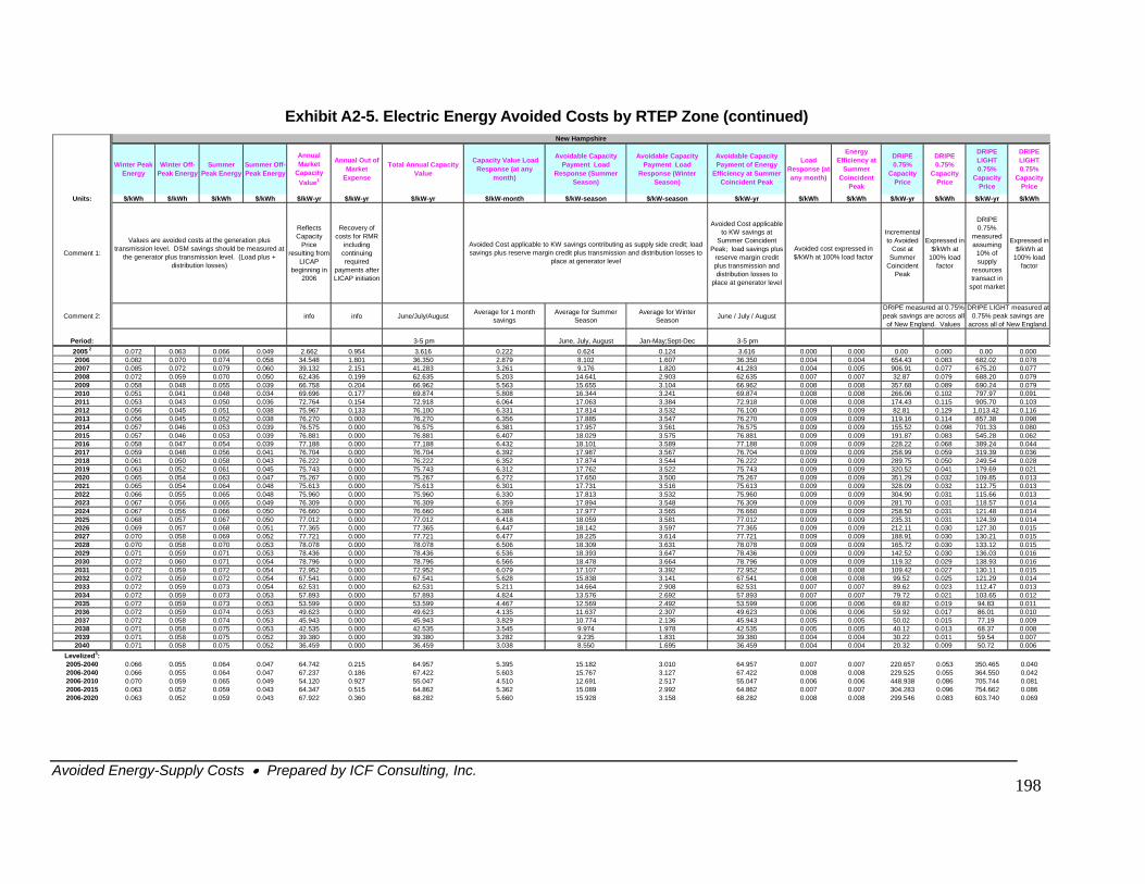
Avoided Energy-Supply Costs • Prepared by ICF Consulting, Inc.
198
Exhibit A2-5. Electric Energy Avoided Costs by RTEP Zone (continued)
Winter Peak Energy
Winter Off-Peak Energy
Summer Peak Energy
Summer Off-Peak Energy
Annual Market
Capacity Value1
Annual Out of Market
Expense
Total Annual Capacity Value
Capacity Value Load Response (at any
month)
Avoidable Capacity Payment Load
Response (Summer Season)
Avoidable Capacity Payment Load
Response (Winter Season)
Avoidable Capacity Payment of Energy
Efficiency at Summer Coincident Peak
Load Response (at any month)
Energy Efficiency at
Summer Coincident
Peak
DRIPE 0.75%
Capacity Price
DRIPE 0.75%
Capacity Price
DRIPE LIGHT 0.75%
Capacity Price
DRIPE LIGHT 0.75%
Capacity Price
Units: $/kWh $/kWh $/kWh $/kWh $/kW-yr $/kW-yr $/kW-yr $/kW-month $/kW-season $/kW-season $/kW-yr $/kWh $/kWh $/kW-yr $/kWh $/kW-yr $/kWh
Comment 1:
Reflects Capacity
Price resulting from
LICAP beginning in
2006
Recovery of costs for RMR
including continuing required
payments after LICAP initiation
Avoided Cost applicable to KW savings at
Summer Coincident Peak; load savings plus
reserve margin credit plus transmission and distribution losses to
place at generator level
Incremental to Avoided
Cost at Summer
Coincident Peak
Expressed in $/kWh at
100% load factor
DRIPE 0.75%
measured assuming
10% of supply
resources transact in
spot market
Expressed in $/kWh at
100% load factor
Comment 2: info info June/July/August Average for 1 month savings
Average for Summer Season
Average for Winter Season June / July / August
Period: 3-5 pm June, July, August Jan-May;Sept-Dec 3-5 pm2005 2 0.072 0.063 0.066 0.049 2.662 0.954 3.616 0.222 0.624 0.124 3.616 0.000 0.000 0.00 0.000 0.00 0.0002006 0.082 0.070 0.074 0.058 34.548 1.801 36.350 2.879 8.102 1.607 36.350 0.004 0.004 654.43 0.083 682.02 0.0782007 0.085 0.072 0.079 0.060 39.132 2.151 41.283 3.261 9.176 1.820 41.283 0.004 0.005 906.91 0.077 675.20 0.0772008 0.072 0.059 0.070 0.050 62.436 0.199 62.635 5.203 14.641 2.903 62.635 0.007 0.007 32.87 0.079 688.20 0.0792009 0.058 0.048 0.055 0.039 66.758 0.204 66.962 5.563 15.655 3.104 66.962 0.008 0.008 357.68 0.089 690.24 0.0792010 0.051 0.041 0.048 0.034 69.696 0.177 69.874 5.808 16.344 3.241 69.874 0.008 0.008 266.06 0.102 797.97 0.0912011 0.053 0.043 0.050 0.036 72.764 0.154 72.918 6.064 17.063 3.384 72.918 0.008 0.008 174.43 0.115 905.70 0.1032012 0.056 0.045 0.051 0.038 75.967 0.133 76.100 6.331 17.814 3.532 76.100 0.009 0.009 82.81 0.129 1,013.42 0.1162013 0.056 0.045 0.052 0.038 76.270 0.000 76.270 6.356 17.885 3.547 76.270 0.009 0.009 119.16 0.114 57.38
098 01.33083 45.28068 89.24059 19.39050 49.54
027 30.11025 1.29
.023 2.47
.021 3.65
.019 83
.017 01
.015 19
.013 37
.011 54
.009 72
.053 .465
.055 .550
.086 .744
.096 .662
8 0.0982014 0.057 0.046 0.053 0.039 76.575 0.000 76.575 6.381 17.957 3.561 76.575 0.009 0.009 155.52 0. 7 0.0802015 0.057 0.046 0.053 0.039 76.881 0.000 76.881 6.407 18.029 3.575 76.881 0.009 0.009 191.87 0. 5 0.0622016 0.058 0.047 0.054 0.039 77.188 0.000 77.188 6.432 18.101 3.589 77.188 0.009 0.009 228.22 0. 3 0.0442017 0.059 0.048 0.056 0.041 76.704 0.000 76.704 6.392 17.987 3.567 76.704 0.009 0.009 258.99 0. 3 0.0362018 0.061 0.050 0.058 0.043 76.222 0.000 76.222 6.352 17.874 3.544 76.222 0.009 0.009 289.75 0. 2 0.0282019 0.063 0.052 0.061 0.045 75.743 0.000 75.743 6.312 17.762 3.522 75.743 0.009 0.009 320.52 0.041 179.69 0.0212020 0.065 0.054 0.063 0.047 75.267 0.000 75.267 6.272 17.650 3.500 75.267 0.009 0.009 351.29 0.032 109.85 0.0132021 0.065 0.054 0.064 0.048 75.613 0.000 75.613 6.301 17.731 3.516 75.613 0.009 0.009 328.09 0.032 112.75 0.0132022 0.066 0.055 0.065 0.048 75.960 0.000 75.960 6.330 17.813 3.532 75.960 0.009 0.009 304.90 0.031 115.66 0.0132023 0.067 0.056 0.065 0.049 76.309 0.000 76.309 6.359 17.894 3.548 76.309 0.009 0.009 281.70 0.031 118.57 0.0142024 0.067 0.056 0.066 0.050 76.660 0.000 76.660 6.388 17.977 3.565 76.660 0.009 0.009 258.50 0.031 121.48 0.0142025 0.068 0.057 0.067 0.050 77.012 0.000 77.012 6.418 18.059 3.581 77.012 0.009 0.009 235.31 0.031 124.39 0.0142026 0.069 0.057 0.068 0.051 77.365 0.000 77.365 6.447 18.142 3.597 77.365 0.009 0.009 212.11 0.030 127.30 0.0152027 0.070 0.058 0.069 0.052 77.721 0.000 77.721 6.477 18.225 3.614 77.721 0.009 0.009 188.91 0.030 130.21 0.0152028 0.070 0.058 0.070 0.053 78.078 0.000 78.078 6.506 18.309 3.631 78.078 0.009 0.009 165.72 0.030 133.12 0.0152029 0.071 0.059 0.071 0.053 78.436 0.000 78.436 6.536 18.393 3.647 78.436 0.009 0.009 142.52 0.030 136.03 0.0162030 0.072 0.060 0.071 0.054 78.796 0.000 78.796 6.566 18.478 3.664 78.796 0.009 0.009 119.32 0.029 138.93 0.0162031 0.072 0.059 0.072 0.054 72.952 0.000 72.952 6.079 17.107 3.392 72.952 0.008 0.008 109.42 0. 1 0.0152032 0.072 0.059 0.072 0.054 67.541 0.000 67.541 5.628 15.838 3.141 67.541 0.008 0.008 99.52 0. 12 0.0142033 0.072 0.059 0.073 0.054 62.531 0.000 62.531 5.211 14.664 2.908 62.531 0.007 0.007 89.62 0 11 0.0132034 0.072 0.059 0.073 0.053 57.893 0.000 57.893 4.824 13.576 2.692 57.893 0.007 0.007 79.72 0 10 0.0122035 0.072 0.059 0.073 0.053 53.599 0.000 53.599 4.467 12.569 2.492 53.599 0.006 0.006 69.82 0 94. 0.0112036 0.072 0.059 0.074 0.053 49.623 0.000 49.623 4.135 11.637 2.307 49.623 0.006 0.006 59.92 0 86. 0.0102037 0.072 0.058 0.074 0.053 45.943 0.000 45.943 3.829 10.774 2.136 45.943 0.005 0.005 50.02 0 77. 0.0092038 0.071 0.058 0.075 0.053 42.535 0.000 42.535 3.545 9.974 1.978 42.535 0.005 0.005 40.12 0 68. 0.0082039 0.071 0.058 0.075 0.052 39.380 0.000 39.380 3.282 9.235 1.831 39.380 0.004 0.004 30.22 0 59. 0.0072040 0.071 0.058 0.075 0.052 36.459 0.000 36.459 3.038 8.550 1.695 36.459 0.004 0.004 20.32 0 50. 0.006
Levelized3: 2005-2040 0.066 0.055 0.064 0.047 64.742 0.215 64.957 5.395 15.182 3.010 64.957 0.007 0.007 220.657 0 350 0.0402006-2040 0.066 0.055 0.064 0.047 67.237 0.186 67.422 5.603 15.767 3.127 67.422 0.008 0.008 229.525 0 364 0.0422006-2010 0.070 0.059 0.065 0.049 54.120 0.927 55.047 4.510 12.691 2.517 55.047 0.006 0.006 448.938 0 705 0.0812006-2015 0.063 0.052 0.059 0.043 64.347 0.515 64.862 5.362 15.089 2.992 64.862 0.007 0.007 304.283 0 754 0.0862006-2020 0.063 0.052 0.059 0.043 67.922 0.360 68.282 5.660 15.928 3.158 68.282 0.008 0.008 299.546 0.083 603.740 0.069
DRIPE LIGHT measured at 0.75% peak savings are
across all of New England.
Values are avoided costs at the generation plus transmission level. DSM savings should be measured at
the generator plus transmission level. (Load plus + distribution losses)
Avoided cost expressed in $/kWh at 100% load factor
DRIPE measured at 0.75% peak savings are across all
of New England. Values
New Hampshire
Avoided Cost applicable to KW savings contributing as supply side credit; load savings plus reserve margin credit plus transmission and distribution losses to
place at generator level
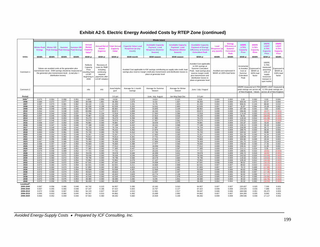
Exhibit A2-5. Electric Energy Avoided Costs by RTEP Zone (continued)
Winter Peak Energy
Winter Off-Peak Energy
Summer Peak Energy
Summer Off-Peak Energy
Annual Market
Capacity Value1
Annual Out of Market
Expense
Total Annual Capacity
Value
Capacity Value Load Response (at any
month)
Avoidable Capacity Payment Load
Response (Summer Season)
Avoidable Capacity Payment Load
Response (Winter Season)
Avoidable Capacity Payment of Energy
Efficiency at Summer Coincident Peak
Load Response (at any month)
Energy Efficiency at
Summer Coincident
Peak
DRIPE 0.75%
Capacity Price
DRIPE 0.75%
Capacity Price
DRIPE LIGHT 0.75%
Capacity Price
DRIPE LIGHT 0.75%
Capacity Price
Units: $/kWh $/kWh $/kWh $/kWh $/kW-yr $/kW-yr $/kW-yr $/kW-month $/kW-season $/kW-season $/kW-yr $/kWh $/kWh $/kW-yr $/kWh $/kW-yr $/kWh
Comment 1:
Reflects Capacity
Price resulting from
LICAP beginning in
2006
Recovery of costs for RMR
including continuing required
payments after LICAP initiation
Avoided Cost applicable to KW savings at
Summer Coincident Peak; load savings plus
reserve margin credit plus transmission and distribution losses to
place at generator level
Incremental to Avoided
Cost at Summer
Coincident Peak
Expressed in $/kWh at
100% load factor
DRIPE 0.75%
measured assuming
10% of supply
resources transact in
spot market
Expressed in $/kWh at
100% load factor
Comment 2: info info June/July/August
Average for 1 month savings
Average for Summer Season
Average for Winter Season June / July / August
Period: 3-5 pm June, July, August Jan-May;Sept-Dec 3-5 pm2005 2 0.073 0.064 0.068 0.051 2.662 0.954 3.616 0.222 0.624 0.124 3.616 0.000 0.000 0.00 0.000 0.00 0.0002006 0.084 0.072 0.077 0.060 34.548 1.801 36.350 2.879 8.102 1.607 36.350 0.004 0.004 654.43 0.075 32.57 0.0042007 0.087 0.074 0.081 0.062 39.132 2.151 41.283 3.261 9.176 1.820 41.283 0.004 0.005 906.91 0.104 88.60 0.0102008 0.074 0.060 0.071 0.051 62.436 0.199 62.635 5.203 14.641 2.903 62.635 0.007 0.007 32.87 0.004 15.28 0.0022009 0.060 0.049 0.056 0.040 66.758 0.204 66.962 5.563 15.655 3.104 66.962 0.008 0.008 357.68 0.041 9.62 0.0012010 0.052 0.042 0.048 0.035 69.696 0.177 69.874 5.808 16.344 3.241 69.874 0.008 0.008 266.06 0.030 (6.87) (0.001)2011 0.054 0.044 0.050 0.037 72.764 0.154 72.918 6.064 17.063 3.384 72.918 0.008 0.008 174.43 0.020 (23.35) (0.003)2012 0.057 0.045 0.052 0.038 75.967 0.133 76.100 6.331 17.814 3.532 76.100 0.009 0.009 82.81 0.009 (39.84) (0.005)2013 0.057 0.046 0.053 0.039 76.270 0.000 76.270 6.356 17.885 3.547 76.270 0.009 0.009 119.16 0.014 (21.08) (0.002)2014 0.057 0.046 0.053 0.039 76.575 0.000 76.575 6.381 17.957 3.561 76.575 0.009 0.009 155.52 0.018 (2.33) (0.000)2015 0.058 0.047 0.054 0.040 76.881 0.000 76.881 6.407 18.029 3.575 76.881 0.009 0.009 191.87 0.022 16.43 0.0022016 0.058 0.047 0.054 0.040 77.188 0.000 77.188 6.432 18.101 3.589 77.188 0.009 0.009 228.22 0.026 35.18 0.0042017 0.060 0.049 0.056 0.042 76.704 0.000 76.704 6.392 17.987 3.567 76.704 0.009 0.009 258.99 0.030 36.72 0.0042018 0.062 0.050 0.059 0.044 76.222 0.000 76.222 6.352 17.874 3.544 76.222 0.009 0.009 289.75 0.033 38.26 0.0042019 0.063 0.052 0.061 0.046 75.743 0.000 75.743 6.312 17.762 3.522 75.743 0.009 0.009 320.52 0.037 39.80 0.0052020 0.065 0.054 0.063 0.048 75.267 0.000 75.267 6.272 17.650 3.500 75.267 0.009 0.009 351.29 0.040 41.34 0.0052021 0.066 0.055 0.064 0.048 75.613 0.000 75.613 6.301 17.731 3.516 75.613 0.009 0.009 328.09 0.037 35.34 0.0042022 0.067 0.055 0.065 0.049 75.960 0.000 75.960 6.330 17.813 3.532 75.960 0.009 0.009 304.90 0.035 29.34 0.0032023 0.067 0.056 0.066 0.050 76.309 0.000 76.309 6.359 17.894 3.548 76.309 0.009 0.009 281.70 0.032 23.34 0.0032024 0.068 0.057 0.067 0.050 76.660 0.000 76.660 6.388 17.977 3.565 76.660 0.009 0.009 258.50 0.030 17.35 0.0022025 0.069 0.057 0.067 0.051 77.012 0.000 77.012 6.418 18.059 3.581 77.012 0.009 0.009 235.31 0.027 11.35 0.0012026 0.069 0.058 0.068 0.052 77.365 0.000 77.365 6.447 18.142 3.597 77.365 0.009 0.009 212.11 0.024 5.35 0.0012027 0.070 0.058 0.069 0.052 77.721 0.000 77.721 6.477 18.225 3.614 77.721 0.009 0.009 188.91 0.022 (0.65) (0.000)2028 0.071 0.059 0.070 0.053 78.078 0.000 78.078 6.506 18.309 3.631 78.078 0.009 0.009 165.72 0.019 (6.65) (0.001)2029 0.072 0.060 0.071 0.054 78.436 0.000 78.436 6.536 18.393 3.647 78.436 0.009 0.009 142.52 0.016 (12.64) (0.001)2030 0.072 0.060 0.072 0.054 78.796 0.000 78.796 6.566 18.478 3.664 78.796 0.009 0.009 119.32 0.014 (18.64) (0.002)2031 0.072 0.060 0.072 0.054 72.952 0.000 72.952 6.079 17.107 3.392 72.952 0.008 0.008 109.42 0.012 (18.43) (0.002)2032 0.072 0.060 0.072 0.054 67.541 0.000 67.541 5.628 15.838 3.141 67.541 0.008 0.008 99.52 0.011 (18.22) (0.002)2033 0.072 0.060 0.073 0.054 62.531 0.000 62.531 5.211 14.664 2.908 62.531 0.007 0.007 89.62 0.010 (18.01) (0.002)2034 0.072 0.060 0.073 0.054 57.893 0.000 57.893 4.824 13.576 2.692 57.893 0.007 0.007 79.72 0.009 (17.80) (0.002)2035 0.072 0.059 0.074 0.054 53.599 0.000 53.599 4.467 12.569 2.492 53.599 0.006 0.006 69.82 0.008 (17.59) (0.002)2036 0.072 0.059 0.074 0.053 49.623 0.000 49.623 4.135 11.637 2.307 49.623 0.006 0.006 59.92 0.007 (17.38) (0.002)2037 0.072 0.059 0.075 0.053 45.943 0.000 45.943 3.829 10.774 2.136 45.943 0.005 0.005 50.02 0.006 (17.17) (0.002)2038 0.072 0.059 0.075 0.053 42.535 0.000 42.535 3.545 9.974 1.978 42.535 0.005 0.005 40.12 0.005 (16.96) (0.002)2039 0.072 0.058 0.075 0.053 39.380 0.000 39.380 3.282 9.235 1.831 39.380 0.004 0.004 30.22 0.003 (16.75) (0.002)2040 0.072 0.058 0.076 0.053 36.459 0.000 36.459 3.038 8.550 1.695 36.459 0.004 0.004 20.32 0.002 (16.54) (0.002)
Levelized3: 2005-2040 0.067 0.056 0.065 0.048 64.742 0.215 64.957 5.395 15.182 3.010 64.957 0.007 0.007 220.657 0.025 7.200 0.0012006-2040 0.067 0.055 0.065 0.048 67.237 0.186 67.422 5.603 15.767 3.127 67.422 0.008 0.008 229.525 0.026 7.489 0.0012006-2010 0.072 0.060 0.067 0.050 54.120 0.927 55.047 4.510 12.691 2.517 55.047 0.006 0.006 448.938 0.051 28.472 0.0032006-2015 0.065 0.053 0.060 0.045 64.347 0.515 64.862 5.362 15.089 2.992 64.862 0.007 0.007 304.283 0.035 8.063 0.0012006-2020 0.064 0.052 0.059 0.044 67.922 0.360 68.282 5.660 15.928 3.158 68.282 0.008 0.008 299.546 0.034 17.117 0.002
Rhode Island
DRIPE LIGHT measured at 0.75% peak savings are
across all of New England.
Avoided Cost applicable to KW savings contributing as supply side credit; load savings plus reserve margin credit plus transmission and distribution losses to
place at generator level
DRIPE measured at 0.75% peak savings are across all
of New England. Values
Values are avoided costs at the generation plus transmission level. DSM savings should be measured at
the generator plus transmission level. (Load plus + distribution losses)
Avoided cost expressed in $/kWh at 100% load factor
Avoided Energy-Supply Costs • Prepared by ICF Consulting, Inc.
199
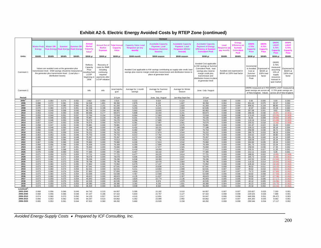
Avoided Energy-Supply Costs • Prepared by ICF Consulting, Inc.
200
Exhibit A2-5. Electric Energy Avoided Costs by RTEP Zone (continued)
Winter Peak Energy
Winter Off-Peak Energy
Summer Peak Energy
Summer Off-Peak Energy
Annual Market
Capacity Value1
Annual Out of Market
Expense
Total Annual Capacity
Value
Capacity Value Load Response (at any
month)
Avoidable Capacity Payment Load
Response (Summer Season)
Avoidable Capacity Payment Load
Response (Winter Season)
Avoidable Capacity Payment of Energy
Efficiency at Summer Coincident Peak
Load Response (at any month)
Energy Efficiency at
Summer Coincident
Peak
DRIPE 0.75%
Capacity Price
DRIPE 0.75%
Capacity Price
DRIPE LIGHT 0.75%
Capacity Price
DRIPE LIGHT 0.75%
Capacity Price
Units: $/kWh $/kWh $/kWh $/kWh $/kW-yr $/kW-yr $/kW-yr $/kW-month $/kW-season $/kW-season $/kW-yr $/kWh $/kWh $/kW-yr $/kWh $/kW-yr $/kWh
Comment 1:
Reflects Capacity
Price resulting from
LICAP beginning in
2006
Recovery of costs for RMR
including continuing required
payments after LICAP initiation
Avoided Cost applicable to KW savings at Summer
Coincident Peak; load savings plus reserve
margin credit plus transmission and
distribution losses to place at generator level
Incremental to Avoided
Cost at Summer
Coincident Peak
Expressed in $/kWh at
100% load factor
DRIPE 0.75%
measured assuming
10% of supply
resources transact in
spot market
Expressed in $/kWh at
100% load factor
Comment 2: info info June/July/August
Average for 1 month savings
Average for Summer Season
Average for Winter Season June / July / August
Period: 3-5 pm June, July, August Jan-May;Sept-Dec 3-5 pm2005 2 0.077 0.064 0.074 0.052 2.662 0.954 3.616 0.222 0.624 0.124 3.616 0.000 0.000 0.00 0.000 0.00 0.0002006 0.088 0.072 0.081 0.061 34.548 1.801 36.350 2.879 8.102 1.607 36.350 0.004 0.004 654.43 0.075 32.57 0.0042007 0.090 0.074 0.085 0.062 39.132 2.151 41.283 3.261 9.176 1.820 41.283 0.004 0.005 906.91 0.104 88.60 0.0102008 0.076 0.060 0.073 0.051 62.436 0.199 62.635 5.203 14.641 2.903 62.635 0.007 0.007 32.87 0.004 15.28 0.0022009 0.062 0.049 0.058 0.040 66.758 0.204 66.962 5.563 15.655 3.104 66.962 0.008 0.008 357.68 0.041 2
30 .87)20 .35)09 .84)14 .08)
8 .33)
24 3522 .65)19 .65)16 .64)14 .64)12 .43)11 .22)10 .01)09 .80)08 .59)07 .38)06 .17)05 .96)03 .75)
9.6 0.0012010 0.053 0.042 0.050 0.035 69.696 0.177 69.874 5.808 16.344 3.241 69.874 0.008 0.008 266.06 0.0 (6 (0.001)2011 0.055 0.044 0.051 0.037 72.764 0.154 72.918 6.064 17.063 3.384 72.918 0.008 0.008 174.43 0.0 (23 (0.003)2012 0.056 0.046 0.052 0.038 75.967 0.133 76.100 6.331 17.814 3.532 76.100 0.009 0.009 82.81 0.0 (39 (0.005)2013 0.057 0.046 0.053 0.039 76.270 0.000 76.270 6.356 17.885 3.547 76.270 0.009 0.009 119.16 0.0 (21 (0.002)2014 0.057 0.047 0.053 0.039 76.575 0.000 76.575 6.381 17.957 3.561 76.575 0.009 0.009 155.52 0.01 (2 (0.000)2015 0.058 0.047 0.054 0.040 76.881 0.000 76.881 6.407 18.029 3.575 76.881 0.009 0.009 191.87 0.022 16.43 0.0022016 0.058 0.048 0.055 0.040 77.188 0.000 77.188 6.432 18.101 3.589 77.188 0.009 0.009 228.22 0.026 35.18 0.0042017 0.060 0.049 0.057 0.042 76.704 0.000 76.704 6.392 17.987 3.567 76.704 0.009 0.009 258.99 0.030 36.72 0.0042018 0.062 0.051 0.059 0.044 76.222 0.000 76.222 6.352 17.874 3.544 76.222 0.009 0.009 289.75 0.033 38.26 0.0042019 0.064 0.053 0.061 0.046 75.743 0.000 75.743 6.312 17.762 3.522 75.743 0.009 0.009 320.52 0.037 39.80 0.0052020 0.065 0.055 0.064 0.048 75.267 0.000 75.267 6.272 17.650 3.500 75.267 0.009 0.009 351.29 0.040 41.34 0.0052021 0.066 0.055 0.065 0.049 75.613 0.000 75.613 6.301 17.731 3.516 75.613 0.009 0.009 328.09 0.037 35.34 0.0042022 0.067 0.056 0.066 0.049 75.960 0.000 75.960 6.330 17.813 3.532 75.960 0.009 0.009 304.90 0.035 29.34 0.0032023 0.068 0.056 0.066 0.050 76.309 0.000 76.309 6.359 17.894 3.548 76.309 0.009 0.009 281.70 0.032 23.34 0.0032024 0.068 0.057 0.067 0.051 76.660 0.000 76.660 6.388 17.977 3.565 76.660 0.009 0.009 258.50 0.030 17.35 0.0022025 0.069 0.058 0.068 0.051 77.012 0.000 77.012 6.418 18.059 3.581 77.012 0.009 0.009 235.31 0.027 11.35 0.0012026 0.070 0.058 0.069 0.052 77.365 0.000 77.365 6.447 18.142 3.597 77.365 0.009 0.009 212.11 0.0 5. 0.0012027 0.071 0.059 0.070 0.053 77.721 0.000 77.721 6.477 18.225 3.614 77.721 0.009 0.009 188.91 0.0 (0 (0.000)2028 0.071 0.059 0.071 0.054 78.078 0.000 78.078 6.506 18.309 3.631 78.078 0.009 0.009 165.72 0.0 (6 (0.001)2029 0.072 0.060 0.072 0.054 78.436 0.000 78.436 6.536 18.393 3.647 78.436 0.009 0.009 142.52 0.0 (12 (0.001)2030 0.073 0.061 0.073 0.055 78.796 0.000 78.796 6.566 18.478 3.664 78.796 0.009 0.009 119.32 0.0 (18 (0.002)2031 0.073 0.060 0.073 0.055 72.952 0.000 72.952 6.079 17.107 3.392 72.952 0.008 0.008 109.42 0.0 (18 (0.002)2032 0.073 0.060 0.073 0.055 67.541 0.000 67.541 5.628 15.838 3.141 67.541 0.008 0.008 99.52 0.0 (18 (0.002)2033 0.073 0.060 0.074 0.054 62.531 0.000 62.531 5.211 14.664 2.908 62.531 0.007 0.007 89.62 0.0 (18 (0.002)2034 0.073 0.060 0.074 0.054 57.893 0.000 57.893 4.824 13.576 2.692 57.893 0.007 0.007 79.72 0.0 (17 (0.002)2035 0.073 0.060 0.075 0.054 53.599 0.000 53.599 4.467 12.569 2.492 53.599 0.006 0.006 69.82 0.0 (17 (0.002)2036 0.073 0.060 0.075 0.054 49.623 0.000 49.623 4.135 11.637 2.307 49.623 0.006 0.006 59.92 0.0 (17 (0.002)2037 0.073 0.059 0.075 0.054 45.943 0.000 45.943 3.829 10.774 2.136 45.943 0.005 0.005 50.02 0.0 (17 (0.002)2038 0.073 0.059 0.076 0.053 42.535 0.000 42.535 3.545 9.974 1.978 42.535 0.005 0.005 40.12 0.0 (16 (0.002)2039 0.073 0.059 0.076 0.053 39.380 0.000 39.380 3.282 9.235 1.831 39.380 0.004 0.004 30.22 0.0 (16 (0.002)2040 0.073 0.059 0.076 0.053 36.459 0.000 36.459 3.038 8.550 1.695 36.459 0.004 0.004 20.32 0.002 (16.54) (0.002)
Levelized3: 2005-2040 0.068 0.056 0.066 0.049 64.742 0.215 64.957 5.395 15.182 3.010 64.957 0.007 0.007 220.657 0.025 7.200 0.0012006-2040 0.068 0.056 0.066 0.048 67.237 0.186 67.422 5.603 15.767 3.127 67.422 0.008 0.008 229.525 0.026 7.489 0.0012006-2010 0.074 0.060 0.070 0.050 54.120 0.927 55.047 4.510 12.691 2.517 55.047 0.006 0.006 448.938 0.051 28.472 0.0032006-2015 0.066 0.053 0.062 0.045 64.347 0.515 64.862 5.362 15.089 2.992 64.862 0.007 0.007 304.283 0.035 8.063 0.0012006-2020 0.065 0.053 0.061 0.044 67.922 0.360 68.282 5.660 15.928 3.158 68.282 0.008 0.008 299.546 0.034 17.117 0.002
Vermont
DRIPE LIGHT measured at 0.75% peak savings are
across all of New England.
DRIPE measured at 0.75% peak savings are across all
of New England. Values
Avoided Cost applicable to KW savings contributing as supply side credit; load savings plus reserve margin credit plus transmission and distribution losses to
place at generator level
Values are avoided costs at the generation plus transmission level. DSM savings should be measured at
the generator plus transmission level. (Load plus + distribution losses)
Avoided cost expressed in $/kWh at 100% load factor
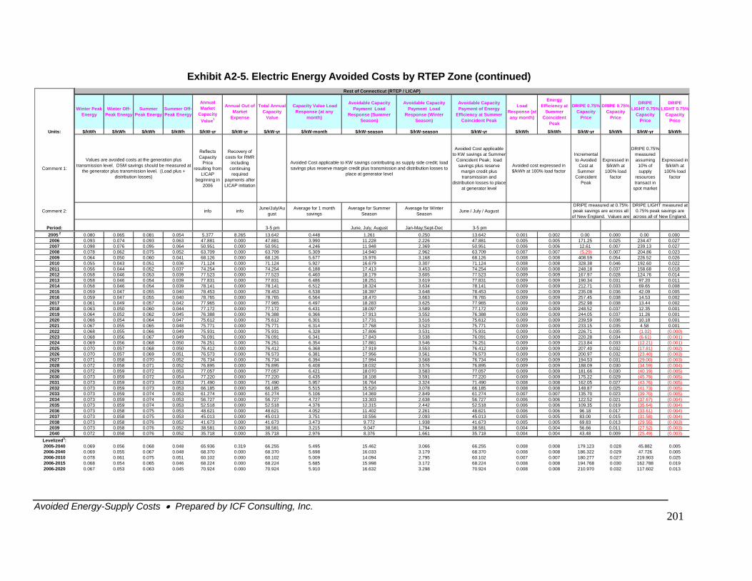
Exhibit A2-5. Electric Energy Avoided Costs by RTEP Zone (continued)
Winter Peak Energy
Winter Off-Peak Energy
Summer Peak Energy
Summer Off-Peak Energy
Annual Market
Capacity Value1
Annual Out of Market
Expense
Total Annual Capacity
Value
Capacity Value Load Response (at any
month)
Avoidable Capacity Payment Load
Response (Summer Season)
Avoidable Capacity Payment Load
Response (Winter Season)
Avoidable Capacity Payment of Energy
Efficiency at Summer Coincident Peak
Load Response (at any month)
Energy Efficiency at
Summer Coincident
Peak
DRIPE 0.75% Capacity
Price
DRIPE 0.75% Capacity
Price
DRIPE LIGHT 0.75%
Capacity Price
DRIPE LIGHT 0.75%
Capacity Price
Units: $/kWh $/kWh $/kWh $/kWh $/kW-yr $/kW-yr $/kW-yr $/kW-month $/kW-season $/kW-season $/kW-yr $/kWh $/kWh $/kW-yr $/kWh $/kW-yr $/kWh
Comment 1:
Reflects Capacity
Price resulting from
LICAP beginning in
2006
Recovery of costs for RMR
including continuing required
payments after LICAP initiation
Avoided Cost applicable to KW savings at Summer
Coincident Peak; load savings plus reserve
margin credit plus transmission and
distribution losses to place at generator level
Incremental to Avoided
Cost at Summer
Coincident Peak
Expressed in $/kWh at
100% load factor
DRIPE 0.75% measured assuming
10% of supply
resources transact in
spot market
Expressed in $/kWh at
100% load factor
Comment 2: info info June/July/August
Average for 1 month savings
Average for Summer Season
Average for Winter Season June / July / August
Period: 3-5 pm June, July, August Jan-May;Sept-Dec 3-5 pm2005 2 0.080 0.065 0.081 0.054 5.377 8.265 13.642 0.448 1.261 0.250 13.642 0.001 0.002 0.00 0.000 0.00 0.0002006 0.093 0.074 0.093 0.063 47.881 0.000 47.881 3.990 11.228 2.226 47.881 0.005 0.005 171.25 0.025 234.47 0.0272007 0.098 0.076 0.095 0.064 50.951 0.000 50.951 4.246 11.948 2.369 50.951 0.006 0.006 12.61 0.007 239.13 0.0272008 0.078 0.062 0.075 0.052 63.709 0.000 63.709 5.309 14.940 2.962 63.709 0.007 0.007 (5.29) 0.007 204.86 0.0232009 0.064 0.050 0.060 0.041 68.126 0.000 68.126 5.677 15.976 3.168 68.126 0.008 0.008 408.59 0.054 226.52 0.0262010 0.055 0.043 0.051 0.036 71.124 0.000 71.124 5.927 16.679 3.307 71.124 0.008 0.008 328.38 0.046 192.60 0.0222011 0.056 0.044 0.052 0.037 74.254 0.000 74.254 6.188 17.413 3.453 74.254 0.008 0.008 248.18 0.037 158.68 0.018
124.76 0.01497.20 0.01169.65 0.00842.09 0.005
29.00) (0.003)(34.59) (0.004)(40.19) (0.005)(45.79) (0.005)(43.76) (0.005)(41.73) (0.005)(39.70) (0.005)(37.67) (0.004)(35.64) (0.004)(33.61) (0.004)(31.58) (0.004)(29.55) (0.003)(27.52) (0.003)(25.49) (0.003)
2012 0.058 0.046 0.053 0.039 77.523 0.000 77.523 6.460 18.179 3.605 77.523 0.009 0.009 167.97 0.0282013 0.058 0.046 0.054 0.039 77.831 0.000 77.831 6.486 18.251 3.619 77.831 0.009 0.009 190.34 0.0312014 0.058 0.046 0.054 0.039 78.141 0.000 78.141 6.512 18.324 3.634 78.141 0.009 0.009 212.71 0.0332015 0.059 0.047 0.055 0.040 78.453 0.000 78.453 6.538 18.397 3.648 78.453 0.009 0.009 235.08 0.0362016 0.059 0.047 0.055 0.040 78.765 0.000 78.765 6.564 18.470 3.663 78.765 0.009 0.009 257.45 0.038 14.53 0.0022017 0.061 0.049 0.057 0.042 77.965 0.000 77.965 6.497 18.283 3.625 77.965 0.009 0.009 252.98 0.038 13.44 0.0022018 0.063 0.050 0.060 0.044 77.172 0.000 77.172 6.431 18.097 3.589 77.172 0.009 0.009 248.52 0.037 12.35 0.0012019 0.064 0.052 0.062 0.045 76.388 0.000 76.388 6.366 17.913 3.552 76.388 0.009 0.009 244.05 0.037 11.26 0.0012020 0.066 0.054 0.064 0.047 75.612 0.000 75.612 6.301 17.731 3.516 75.612 0.009 0.009 239.59 0.036 10.18 0.0012021 0.067 0.055 0.065 0.048 75.771 0.000 75.771 6.314 17.768 3.523 75.771 0.009 0.009 233.15 0.035 4.58 0.0012022 0.068 0.055 0.066 0.049 75.931 0.000 75.931 6.328 17.806 3.531 75.931 0.009 0.009 226.71 0.035 (1.02) (0.000)2023 0.068 0.056 0.067 0.049 76.091 0.000 76.091 6.341 17.843 3.538 76.091 0.009 0.009 220.28 0.034 (6.61) (0.001)2024 0.069 0.056 0.068 0.050 76.251 0.000 76.251 6.354 17.881 3.546 76.251 0.009 0.009 213.84 0.033 (12.21) (0.001)2025 0.070 0.057 0.068 0.050 76.412 0.000 76.412 6.368 17.919 3.553 76.412 0.009 0.009 207.40 0.032 (17.81) (0.002)2026 0.070 0.057 0.069 0.051 76.573 0.000 76.573 6.381 17.956 3.561 76.573 0.009 0.009 200.97 0.032 (23.40) (0.003)2027 0.071 0.058 0.070 0.052 76.734 0.000 76.734 6.394 17.994 3.568 76.734 0.009 0.009 194.53 0.031 (2028 0.072 0.058 0.071 0.052 76.895 0.000 76.895 6.408 18.032 3.576 76.895 0.009 0.009 188.09 0.0302029 0.072 0.059 0.072 0.053 77.057 0.000 77.057 6.421 18.070 3.583 77.057 0.009 0.009 181.66 0.0302030 0.073 0.059 0.072 0.054 77.220 0.000 77.220 6.435 18.108 3.591 77.220 0.009 0.009 175.22 0.0292031 0.073 0.059 0.073 0.053 71.490 0.000 71.490 5.957 16.764 3.324 71.490 0.008 0.008 162.05 0.0272032 0.073 0.059 0.073 0.053 66.185 0.000 66.185 5.515 15.520 3.078 66.185 0.008 0.008 148.87 0.0252033 0.073 0.059 0.074 0.053 61.274 0.000 61.274 5.106 14.369 2.849 61.274 0.007 0.007 135.70 0.0232034 0.073 0.059 0.074 0.053 56.727 0.000 56.727 4.727 13.303 2.638 56.727 0.006 0.006 122.52 0.0212035 0.073 0.059 0.074 0.053 52.518 0.000 52.518 4.376 12.315 2.442 52.518 0.006 0.006 109.35 0.0192036 0.073 0.058 0.075 0.053 48.621 0.000 48.621 4.052 11.402 2.261 48.621 0.006 0.006 96.18 0.0172037 0.073 0.058 0.075 0.053 45.013 0.000 45.013 3.751 10.556 2.093 45.013 0.005 0.005 83.00 0.0152038 0.073 0.058 0.076 0.052 41.673 0.000 41.673 3.473 9.772 1.938 41.673 0.005 0.005 69.83 0.0132039 0.073 0.058 0.076 0.052 38.581 0.000 38.581 3.215 9.047 1.794 38.581 0.004 0.004 56.66 0.0112040 0.072 0.058 0.076 0.052 35.718 0.000 35.718 2.976 8.376 1.661 35.718 0.004 0.004 43.48 0.009
Levelized3: 2005-2040 0.069 0.056 0.068 0.048 65.936 0.319 66.255 5.495 15.462 3.066 66.255 0.008 0.008 179.123 0.028 45.882 0.0052006-2040 0.069 0.055 0.067 0.048 68.370 0.000 68.370 5.698 16.033 3.179 68.370 0.008 0.008 186.322 0.029 47.726 0.0052006-2010 0.078 0.061 0.075 0.051 60.102 0.000 60.102 5.009 14.094 2.795 60.102 0.007 0.007 180.277 0.027 219.903 0.0252006-2015 0.068 0.054 0.065 0.046 68.224 0.000 68.224 5.685 15.998 3.172 68.224 0.008 0.008 194.768 0.030 162.788 0.0192006-2020 0.067 0.053 0.063 0.045 70.924 0.000 70.924 5.910 16.632 3.298 70.924 0.008 0.008 210.970 0.032 117.602 0.013
Rest of Connecticut (RTEP / LICAP)
DRIPE LIGHT measured at 0.75% peak savings are
across all of New England.
Avoided cost expressed in $/kWh at 100% load factor
DRIPE measured at 0.75% peak savings are across all
of New England. Values are
Values are avoided costs at the generation plus transmission level. DSM savings should be measured at
the generator plus transmission level. (Load plus + distribution losses)
Avoided Cost applicable to KW savings contributing as supply side credit; load savings plus reserve margin credit plus transmission and distribution losses to
place at generator level
Avoided Energy-Supply Costs • Prepared by ICF Consulting, Inc.
201
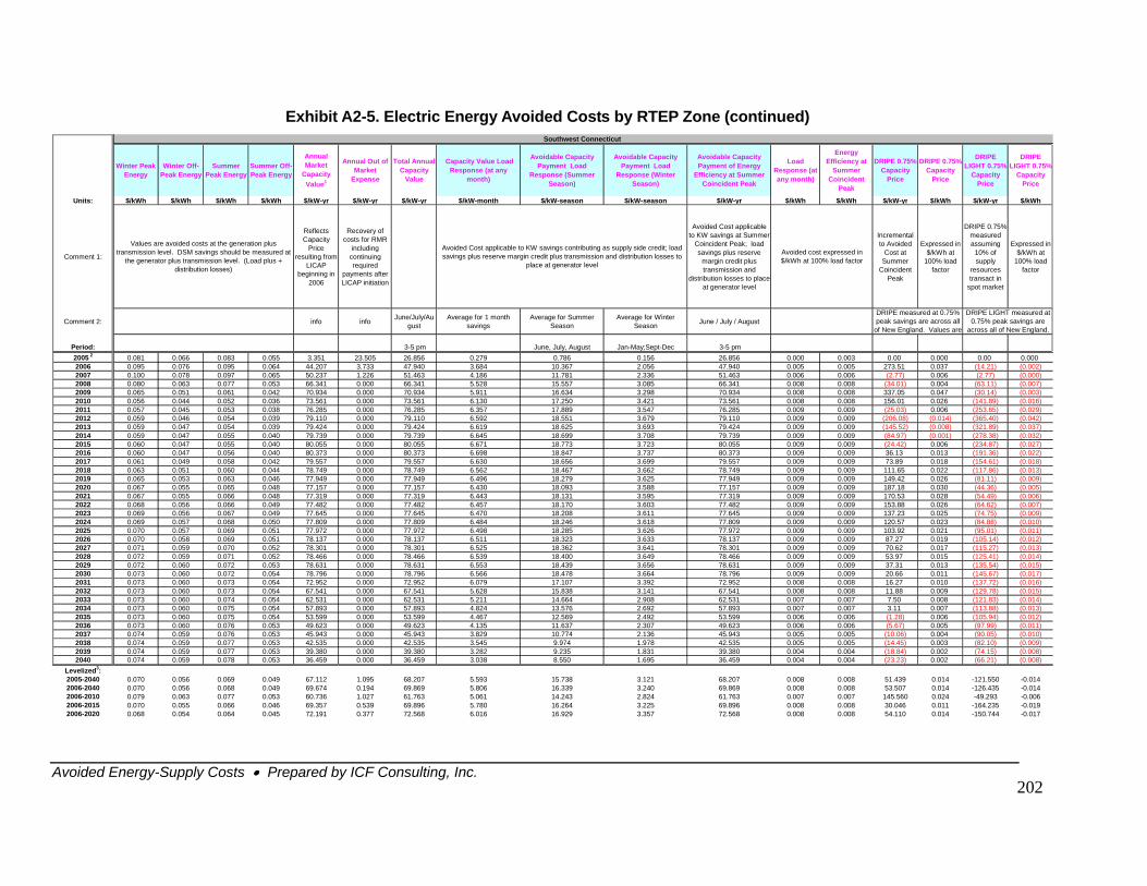
Exhibit A2-5. Electric Energy Avoided Costs by RTEP Zone (continued)
Winter Peak Energy
Winter Off-Peak Energy
Summer Peak Energy
Summer Off-Peak Energy
Annual Market
Capacity Value1
Annual Out of Market
Expense
Total Annual Capacity
Value
Capacity Value Load Response (at any
month)
Avoidable Capacity Payment Load
Response (Summer Season)
Avoidable Capacity Payment Load
Response (Winter Season)
Avoidable Capacity Payment of Energy
Efficiency at Summer Coincident Peak
Load Response (at any month)
Energy Efficiency at
Summer Coincident
Peak
DRIPE 0.75% Capacity
Price
DRIPE 0.75% Capacity
Price
DRIPE LIGHT 0.75%
Capacity Price
DRIPE LIGHT 0.75%
Capacity Price
Units: $/kWh $/kWh $/kWh $/kWh $/kW-yr $/kW-yr $/kW-yr $/kW-month $/kW-season $/kW-season $/kW-yr $/kWh $/kWh $/kW-yr $/kWh $/kW-yr $/kWh
Comment 1:
Reflects Capacity
Price resulting from
LICAP beginning in
2006
Recovery of costs for RMR
including continuing required
payments after LICAP initiation
Avoided Cost applicable to KW savings at Summer
Coincident Peak; load savings plus reserve
margin credit plus transmission and
distribution losses to place at generator level
Incremental to Avoided
Cost at Summer
Coincident Peak
Expressed in $/kWh at
100% load factor
DRIPE 0.75% measured assuming
10% of supply
resources transact in
spot market
Expressed in $/kWh at
100% load factor
Comment 2: info info June/July/August
Average for 1 month savings
Average for Summer Season
Average for Winter Season June / July / August
Period: 3-5 pm June, July, August Jan-May;Sept-Dec 3-5 pm2005 2 0.081 0.066 0.083 0.055 3.351 23.505 26.856 0.279 0.786 0.156 26.856 0.000 0.003 0.00 0.000 0.00 0.0002006 0.095 0.076 0.095 0.064 44.207 3.733 47.940 3.684 10.367 2.056 47.940 0.005 0.005 273.51 0.037 (14.21) (0.002)2007 0.100 0.078 0.097 0.065 50.237 1.226 51.463 4.186 11.781 2.336 51.463 0.006 0.006 (2.77) 0.006 (2.77) (0.000)2008 0.080 0.063 0.077 0.053 66.341 0.000 66.341 5.528 15.557 3.085 66.341 0.008 0.008 (34.01)
337.05
(64.62) (0.007)(74.75) (0.009)(84.88) (0.010)(95.01) (0.011)(105.14) (0.012)(115.27) (0.013)(125.41) (0.014)(135.54) (0.015)(145.67) (0.017)(137.72) (0.016)(129.78) (0.015)(121.83) (0.014)(113.88) (0.013)(105.94) (0.012)(97.99) (0.011)(90.05) (0.010)(82.10) (0.009)(74.15) (0.008)(66.21) (0.008)
0.004 (63.11) (0.007)2009 0.065 0.051 0.061 0.042 70.934 0.000 70.934 5.911 16.634 3.298 70.934 0.008 0.008 0.047 (30.14) (0.003)2010 0.056 0.044 0.052 0.036 73.561 0.000 73.561 6.130 17.250 3.421 73.561 0.008 0.008 156.01 0.026 (141.89) (0.016)2011 0.057 0.045 0.053 0.038 76.285 0.000 76.285 6.357 17.889 3.547 76.285 0.009 0.009 (25.03) 0.006 (253.65) (0.029)2012 0.059 0.046 0.054 0.039 79.110 0.000 79.110 6.592 18.551 3.679 79.110 0.009 0.009 (206.08) (0.014) (365.40) (0.042)2013 0.059 0.047 0.054 0.039 79.424 0.000 79.424 6.619 18.625 3.693 79.424 0.009 0.009 (145.52) (0.008) (321.89) (0.037)2014 0.059 0.047 0.055 0.040 79.739 0.000 79.739 6.645 18.699 3.708 79.739 0.009 0.009 (84.97) (0.001) (278.38) (0.032)2015 0.060 0.047 0.055 0.040 80.055 0.000 80.055 6.671 18.773 3.723 80.055 0.009 0.009 (24.42) 0.006 (234.87) (0.027)2016 0.060 0.047 0.056 0.040 80.373 0.000 80.373 6.698 18.847 3.737 80.373 0.009 0.009 36.13 0.013 (191.36) (0.022)2017 0.061 0.049 0.058 0.042 79.557 0.000 79.557 6.630 18.656 3.699 79.557 0.009 0.009 73.89 0.018 (154.61) (0.018)2018 0.063 0.051 0.060 0.044 78.749 0.000 78.749 6.562 18.467 3.662 78.749 0.009 0.009 111.65 0.022 (117.86) (0.013)2019 0.065 0.053 0.063 0.046 77.949 0.000 77.949 6.496 18.279 3.625 77.949 0.009 0.009 149.42 0.026 (81.11) (0.009)2020 0.067 0.055 0.065 0.048 77.157 0.000 77.157 6.430 18.093 3.588 77.157 0.009 0.009 187.18 0.030 (44.36) (0.005)2021 0.067 0.055 0.066 0.048 77.319 0.000 77.319 6.443 18.131 3.595 77.319 0.009 0.009 170.53 0.028 (54.49) (0.006)2022 0.068 0.056 0.066 0.049 77.482 0.000 77.482 6.457 18.170 3.603 77.482 0.009 0.009 153.88 0.0262023 0.069 0.056 0.067 0.049 77.645 0.000 77.645 6.470 18.208 3.611 77.645 0.009 0.009 137.23 0.0252024 0.069 0.057 0.068 0.050 77.809 0.000 77.809 6.484 18.246 3.618 77.809 0.009 0.009 120.57 0.0232025 0.070 0.057 0.069 0.051 77.972 0.000 77.972 6.498 18.285 3.626 77.972 0.009 0.009 103.92 0.0212026 0.070 0.058 0.069 0.051 78.137 0.000 78.137 6.511 18.323 3.633 78.137 0.009 0.009 87.27 0.0192027 0.071 0.059 0.070 0.052 78.301 0.000 78.301 6.525 18.362 3.641 78.301 0.009 0.009 70.62 0.0172028 0.072 0.059 0.071 0.052 78.466 0.000 78.466 6.539 18.400 3.649 78.466 0.009 0.009 53.97 0.0152029 0.072 0.060 0.072 0.053 78.631 0.000 78.631 6.553 18.439 3.656 78.631 0.009 0.009 37.31 0.0132030 0.073 0.060 0.072 0.054 78.796 0.000 78.796 6.566 18.478 3.664 78.796 0.009 0.009 20.66 0.0112031 0.073 0.060 0.073 0.054 72.952 0.000 72.952 6.079 17.107 3.392 72.952 0.008 0.008 16.27 0.0102032 0.073 0.060 0.073 0.054 67.541 0.000 67.541 5.628 15.838 3.141 67.541 0.008 0.008 11.88 0.0092033 0.073 0.060 0.074 0.054 62.531 0.000 62.531 5.211 14.664 2.908 62.531 0.007 0.007 7.50 0.0082034 0.073 0.060 0.075 0.054 57.893 0.000 57.893 4.824 13.576 2.692 57.893 0.007 0.007 3.11 0.0072035 0.073 0.060 0.075 0.054 53.599 0.000 53.599 4.467 12.569 2.492 53.599 0.006 0.006 (1.28) 0.0062036 0.073 0.060 0.076 0.053 49.623 0.000 49.623 4.135 11.637 2.307 49.623 0.006 0.006 (5.67) 0.0052037 0.074 0.059 0.076 0.053 45.943 0.000 45.943 3.829 10.774 2.136 45.943 0.005 0.005 (10.06) 0.0042038 0.074 0.059 0.077 0.053 42.535 0.000 42.535 3.545 9.974 1.978 42.535 0.005 0.005 (14.45) 0.0032039 0.074 0.059 0.077 0.053 39.380 0.000 39.380 3.282 9.235 1.831 39.380 0.004 0.004 (18.84) 0.0022040 0.074 0.059 0.078 0.053 36.459 0.000 36.459 3.038 8.550 1.695 36.459 0.004 0.004 (23.23) 0.002
Levelized3: 2005-2040 0.070 0.056 0.069 0.049 67.112 1.095 68.207 5.593 15.738 3.121 68.207 0.008 0.008 51.439 0.014 -121.550 -0.0142006-2040 0.070 0.056 0.068 0.049 69.674 0.194 69.869 5.806 16.339 3.240 69.869 0.008 0.008 53.507 0.014 -126.435 -0.0142006-2010 0.079 0.063 0.077 0.053 60.736 1.027 61.763 5.061 14.243 2.824 61.763 0.007 0.007 145.560 0.024 -49.293 -0.0062006-2015 0.070 0.055 0.066 0.046 69.357 0.539 69.896 5.780 16.264 3.225 69.896 0.008 0.008 30.046 0.011 -164.235 -0.0192006-2020 0.068 0.054 0.064 0.045 72.191 0.377 72.568 6.016 16.929 3.357 72.568 0.008 0.008 54.110 0.014 -150.744 -0.017
Southwest Connecticut
DRIPE LIGHT measured at 0.75% peak savings are
across all of New England.
DRIPE measured at 0.75% peak savings are across all
of New England. Values are
Values are avoided costs at the generation plus transmission level. DSM savings should be measured at
the generator plus transmission level. (Load plus + distribution losses)
Avoided cost expressed in $/kWh at 100% load factor
Avoided Cost applicable to KW savings contributing as supply side credit; load savings plus reserve margin credit plus transmission and distribution losses to
place at generator level
Avoided Energy-Supply Costs • Prepared by ICF Consulting, Inc.
202
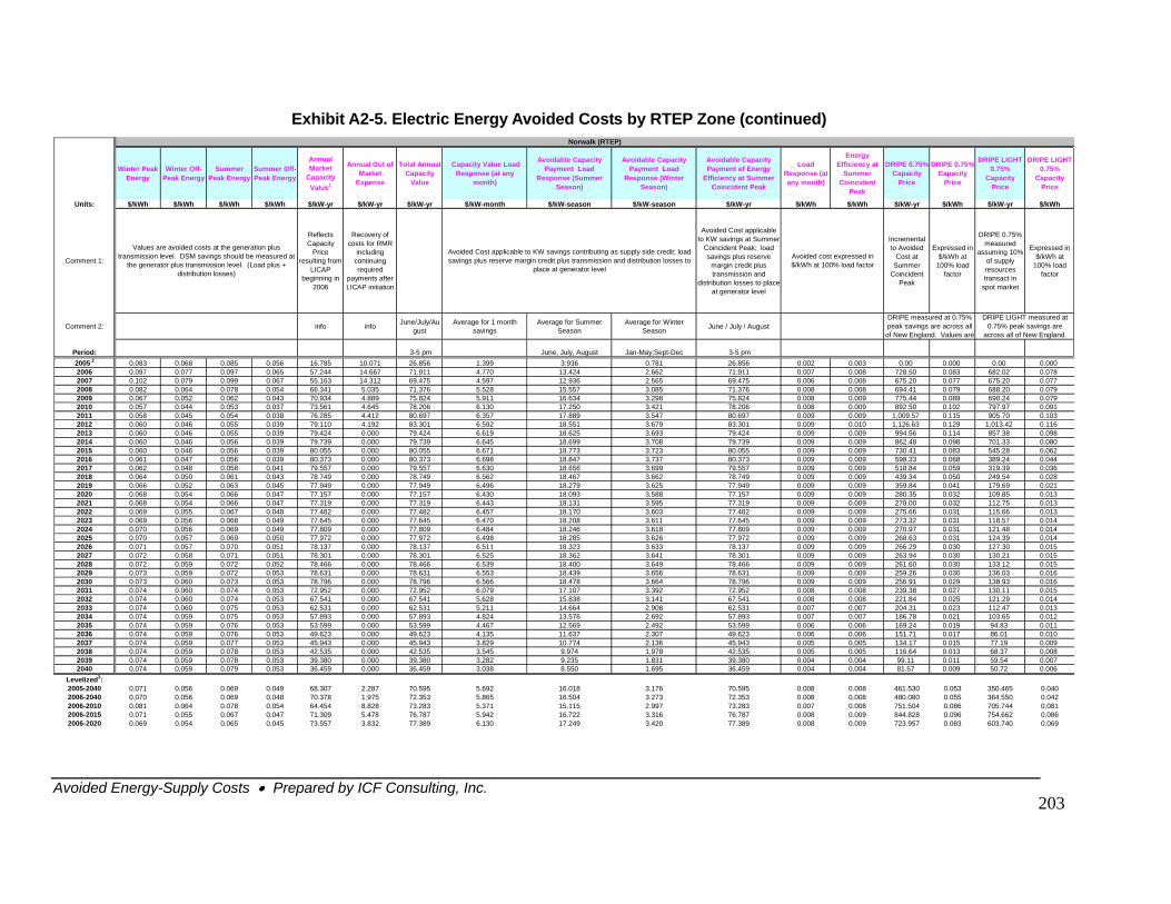
Exhibit A2-5. Electric Energy Avoided Costs by RTEP Zone (continued)
Winter Peak Energy
Winter Off-Peak Energy
Summer Peak Energy
Summer Off-Peak Energy
Annual Market
Capacity Value1
Annual Out of Market
Expense
Total Annual Capacity
Value
Capacity Value Load Response (at any
month)
Avoidable Capacity Payment Load
Response (Summer Season)
Avoidable Capacity Payment Load
Response (Winter Season)
Avoidable Capacity Payment of Energy
Efficiency at Summer Coincident Peak
Load Response (at any month)
Energy Efficiency at
Summer Coincident
Peak
DRIPE 0.75% Capacity
Price
DRIPE 0.75% Capacity
Price
DRIPE LIGHT 0.75%
Capacity Price
DRIPE LIGHT 0.75%
Capacity Price
Units: $/kWh $/kWh $/kWh $/kWh $/kW-yr $/kW-yr $/kW-yr $/kW-month $/kW-season $/kW-season $/kW-yr $/kWh $/kWh $/kW-yr $/kWh $/kW-yr $/kWh
Comment 1:
Reflects Capacity
Price resulting from
LICAP beginning in
2006
Recovery of costs for RMR
including continuing required
payments after LICAP initiation
Avoided Cost applicable to KW savings at Summer
Coincident Peak; load savings plus reserve
margin credit plus transmission and
distribution losses to place at generator level
Incremental to Avoided
Cost at Summer
Coincident Peak
Expressed in $/kWh at
100% load factor
DRIPE 0.75% measured
assuming 10% of supply resources transact in
spot market
Expressed in $/kWh at
100% load factor
Comment 2: info info June/July/August
Average for 1 month savings
Average for Summer Season
Average for Winter Season June / July / August
Period: 3-5 pm June, July, August Jan-May;Sept-Dec 3-5 pm2005 2 0.083 0.068 0.085 0.056 16.785 10.071 26.856 1.399 3.936 0.781 26.856 0.002 0.003 0.00 0.000 0.00 0.0002006 0.097 0.077 0.097 0.065 57.244 14.667 71.911 4.770 13.424 2.662 71.911 0.007 0.008 728.50 0.083 682.02 0.078
75.20 75.20 0.07794.41 88.20 0.079
775.44 90.24 0.07997.97 0.091
09.57 905.70 0.103126.63 129 ,013.42 0.11694.56 .114 857.38 0.09862.48 .098 701.33 0.08030.41 0.083 545.28 0.062
598.33 389.24 0.044319.39 0.036249.54 0.028179.69 0.02109.85 0.01312.75 0.01315.66 0.01318.57 0.01421.48 0.01424.39 0.01427.30 0.015
130.21 0.015133.12 0.015136.03 0.016138.93 0.016130.11 0.015121.29 0.014112.47 0.013103.65 0.012
9.24 94.83 0.01151.71 86.01 0.01034.17 77.19 0.00916.64 68.37 0.0089.11 59.54 0.0071.57 50.72 0.006
2007 0.102 0.079 0.099 0.067 55.163 14.312 69.475 4.597 12.936 2.565 69.475 0.006 0.008 6 0.077 62008 0.082 0.064 0.078 0.054 66.341 5.035 71.376 5.528 15.557 3.085 71.376 0.008 0.008 6 0.079 62009 0.067 0.052 0.062 0.043 70.934 4.889 75.824 5.911 16.634 3.298 75.824 0.008 0.009 0.089 62010 0.057 0.044 0.053 0.037 73.561 4.645 78.206 6.130 17.250 3.421 78.206 0.008 0.009 892.50 0.102 72011 0.058 0.045 0.054 0.038 76.285 4.412 80.697 6.357 17.889 3.547 80.697 0.009 0.009 1,0 0.1152012 0.060 0.046 0.055 0.039 79.110 4.192 83.301 6.592 18.551 3.679 83.301 0.009 0.010 1, 0. 12013 0.060 0.046 0.055 0.039 79.424 0.000 79.424 6.619 18.625 3.693 79.424 0.009 0.009 9 02014 0.060 0.046 0.056 0.039 79.739 0.000 79.739 6.645 18.699 3.708 79.739 0.009 0.009 8 02015 0.060 0.046 0.056 0.039 80.055 0.000 80.055 6.671 18.773 3.723 80.055 0.009 0.009 72016 0.061 0.047 0.056 0.039 80.373 0.000 80.373 6.698 18.847 3.737 80.373 0.009 0.009 0.0682017 0.062 0.048 0.058 0.041 79.557 0.000 79.557 6.630 18.656 3.699 79.557 0.009 0.009 518.84 0.0592018 0.064 0.050 0.061 0.043 78.749 0.000 78.749 6.562 18.467 3.662 78.749 0.009 0.009 439.34 0.0502019 0.066 0.052 0.063 0.045 77.949 0.000 77.949 6.496 18.279 3.625 77.949 0.009 0.009 359.84 0.0412020 0.068 0.054 0.066 0.047 77.157 0.000 77.157 6.430 18.093 3.588 77.157 0.009 0.009 280.35 0.032 12021 0.068 0.054 0.066 0.047 77.319 0.000 77.319 6.443 18.131 3.595 77.319 0.009 0.009 278.00 0.032 12022 0.069 0.055 0.067 0.048 77.482 0.000 77.482 6.457 18.170 3.603 77.482 0.009 0.009 275.66 0.031 12023 0.069 0.056 0.068 0.049 77.645 0.000 77.645 6.470 18.208 3.611 77.645 0.009 0.009 273.32 0.031 12024 0.070 0.056 0.069 0.049 77.809 0.000 77.809 6.484 18.246 3.618 77.809 0.009 0.009 270.97 0.031 12025 0.070 0.057 0.069 0.050 77.972 0.000 77.972 6.498 18.285 3.626 77.972 0.009 0.009 268.63 0.031 12026 0.071 0.057 0.070 0.051 78.137 0.000 78.137 6.511 18.323 3.633 78.137 0.009 0.009 266.29 0.030 12027 0.072 0.058 0.071 0.051 78.301 0.000 78.301 6.525 18.362 3.641 78.301 0.009 0.009 263.94 0.0302028 0.072 0.059 0.072 0.052 78.466 0.000 78.466 6.539 18.400 3.649 78.466 0.009 0.009 261.60 0.0302029 0.073 0.059 0.072 0.053 78.631 0.000 78.631 6.553 18.439 3.656 78.631 0.009 0.009 259.26 0.0302030 0.073 0.060 0.073 0.053 78.796 0.000 78.796 6.566 18.478 3.664 78.796 0.009 0.009 256.91 0.0292031 0.074 0.060 0.074 0.053 72.952 0.000 72.952 6.079 17.107 3.392 72.952 0.008 0.008 239.38 0.0272032 0.074 0.060 0.074 0.053 67.541 0.000 67.541 5.628 15.838 3.141 67.541 0.008 0.008 221.84 0.0252033 0.074 0.060 0.075 0.053 62.531 0.000 62.531 5.211 14.664 2.908 62.531 0.007 0.007 204.31 0.0232034 0.074 0.059 0.075 0.053 57.893 0.000 57.893 4.824 13.576 2.692 57.893 0.007 0.007 186.78 0.0212035 0.074 0.059 0.076 0.053 53.599 0.000 53.599 4.467 12.569 2.492 53.599 0.006 0.006 16 0.0192036 0.074 0.059 0.076 0.053 49.623 0.000 49.623 4.135 11.637 2.307 49.623 0.006 0.006 1 0.0172037 0.074 0.059 0.077 0.053 45.943 0.000 45.943 3.829 10.774 2.136 45.943 0.005 0.005 1 0.0152038 0.074 0.059 0.078 0.053 42.535 0.000 42.535 3.545 9.974 1.978 42.535 0.005 0.005 1 0.0132039 0.074 0.059 0.078 0.053 39.380 0.000 39.380 3.282 9.235 1.831 39.380 0.004 0.004 9 0.0112040 0.074 0.059 0.079 0.053 36.459 0.000 36.459 3.038 8.550 1.695 36.459 0.004 0.004 8 0.009
Levelized3: 2005-2040 0.071 0.056 0.069 0.049 68.307 2.287 70.595 5.692 16.018 3.176 70.595 0.008 0.008 461.530 0.053 350.465 0.0402006-2040 0.070 0.056 0.069 0.048 70.378 1.975 72.353 5.865 16.504 3.273 72.353 0.008 0.008 480.080 0.055 364.550 0.0422006-2010 0.081 0.064 0.078 0.054 64.454 8.828 73.283 5.371 15.115 2.997 73.283 0.007 0.008 751.504 0.086 705.744 0.0812006-2015 0.071 0.055 0.067 0.047 71.309 5.478 76.787 5.942 16.722 3.316 76.787 0.008 0.009 844.828 0.096 754.662 0.0862006-2020 0.069 0.054 0.065 0.045 73.557 3.832 77.389 6.130 17.249 3.420 77.389 0.008 0.009 723.957 0.083 603.740 0.069
DRIPE LIGHT measured at 0.75% peak savings are
across all of New England.
DRIPE measured at 0.75% peak savings are across all
of New England. Values are
Avoided cost expressed in $/kWh at 100% load factor
Values are avoided costs at the generation plus transmission level. DSM savings should be measured at
the generator plus transmission level. (Load plus + distribution losses)
Avoided Cost applicable to KW savings contributing as supply side credit; load savings plus reserve margin credit plus transmission and distribution losses to
place at generator level
Norwalk (RTEP)
Avoided Energy-Supply Costs • Prepared by ICF Consulting, Inc.
203
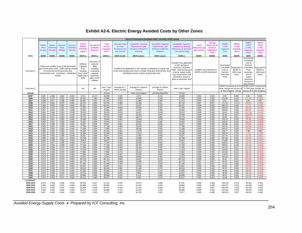
Exhibit A2-6. Electric Energy Avoided Costs by Other Zones
Winter Peak
Energy
Winter Off-Peak Energy
Summer Peak
Energy
Summer Off-Peak Energy
Annual Market
Capacity Value1
Annual Out of Market Expense
Total Annual
Capacity Value
Capacity Value at Load
Response (at any month)
Avoidable Capacity Payment at Load
Response (Summer Season)
Avoidable Capacity Payment at Load Response (Winter
Season)
Avoidable Capacity Payment at Energy
Efficiency at Summer Coincident Peak
Load Response (at any month)
Energy Efficiency at
Summer Coincident
Peak
DRIPE 0.75%
Capacity Price
DRIPE 0.75%
Capacity Price
DRIPE LIGHT 0.75%
Capacity Price
DRIPE LIGHT 0.75%
Capacity Price
Units: $/kWh $/kWh $/kWh $/kWh $/kW-yr $/kW-yr $/kW-yr $/kW-month $/kW-season $/kW-season $/kW-yr $/kWh $/kWh $/kW $/kWh $/kW $/kWh
Comment 1:
Reflects Capacity
Price resulting
from LICAP beginning in
2006
Recovery of costs for
RMR including
continuing required
payments after LICAP
initiation
Avoided Cost applicable to KW savings at
Summer Coincident Peak; load savings plus
reserve margin credit plus transmission and distribution losses to
place at generator level
Incremental to Avoided
Cost at Summer
Coincident Peak
Expressed in $/kWh at
100% load factor
Incremental to Avoided
Cost at Summer
Coincident Peak;
Assumes 10% of supply
resources transact in
spot market
Expressed in $/kWh at
100% load factor
Comment 2: info info June / July / August
Average for 1 month savings
Average for Summer Season
Average for Winter Season June / July / August
Period: 3-5 pm June, July, August Jan-May;Sept-Dec 3-5 pm2005 2 0.081 0.066 0.082 0.054 4.572 14.317 18.889 0.381 1.072 0.213 18.889 0.001 0.002 0.00 0.000 0.00 0.0002006 0.094 0.075 0.094 0.063 46.422 1.483 47.905 3.869 10.886 2.159 47.905 0.005 0.005 211.86 0.024 (21.30) (0.002)2007 0.098 0.077 0.096 0.065 50.667 0.487 51.154 4.222 11.882 2.356 51.154 0.006 0.006 6.50 0.001 6.50 0.0012008 0.079 0.062 0.076 0.052 64.754 0.000 64.754 5.396 15.185 3.011 64.754 0.007 0.007 (16.69) (0.002) (39.97) (0.005)2009 0.064 0.050 0.060 0.042 69.241 0.000 69.241 5.770 16.237 3.220 69.241 0.008 0.008 380.18 0.043 (2.76) (0.000)2010 0.055 0.043 0.051 0.036 72.093 0.000 72.093 6.008 16.906 3.352 72.093 0.008 0.008 259.93 0.030 (44.29) (0.005)2011 0.057 0.045 0.052 0.038 75.062 0.000 75.062 6.255 17.602 3.490 75.062 0.009 0.009 139.68 0.016 (85.82) (0.010)2012 0.058 0.046 0.053 0.039 78.153 0.000 78.153 6.513 18.327 3.634 78.153 0.009 0.009 19.43 0.002 (127.35) (0.015)2013 0.058 0.046 0.054 0.039 78.464 0.000 78.464 6.539 18.400 3.649 78.464 0.009 0.009 56.96 0.007 (108.36) (0.012)2014 0.059 0.047 0.054 0.040 78.776 0.000 78.776 6.565 18.473 3.663 78.776 0.009 0.009 94.49 0.011 (89.37) (0.010)2015 0.059 0.047 0.055 0.040 79.089 0.000 79.089 6.591 18.546 3.678 79.089 0.009 0.009 132.02 0.015 (70.38) (0.008)2016 0.059 0.047 0.055 0.040 79.404 0.000 79.404 6.617 18.620 3.692 79.404 0.009 0.009 169.55 0.019 (51.39) (0.006)2017 0.061 0.049 0.058 0.042 78.597 0.000 78.597 6.550 18.431 3.655 78.597 0.009 0.009 181.86 0.021 (37.82) (0.004)2018 0.063 0.051 0.060 0.044 77.798 0.000 77.798 6.483 18.244 3.618 77.798 0.009 0.009 194.16 0.022 (24.26) (0.003)2019 0.065 0.052 0.062 0.045 77.008 0.000 77.008 6.417 18.058 3.581 77.008 0.009 0.009 206.47 0.024 (10.69) (0.001)2020 0.066 0.054 0.065 0.047 76.226 0.000 76.226 6.352 17.875 3.544 76.226 0.009 0.009 218.77 0.025 2.88 0.0002021 0.067 0.055 0.065 0.048 76.386 0.000 76.386 6.366 17.913 3.552 76.386 0.009 0.009 208.28 0.024 (1.46) (0.000)2022 0.068 0.055 0.066 0.049 76.547 0.000 76.547 6.379 17.950 3.559 76.547 0.009 0.009 197.79 0.023 (5.79) (0.001)2023 0.068 0.056 0.067 0.049 76.708 0.000 76.708 6.392 17.988 3.567 76.708 0.009 0.009 187.29 0.021 (10.13) (0.001)2024 0.069 0.056 0.068 0.050 76.870 0.000 76.870 6.406 18.026 3.574 76.870 0.009 0.009 176.80 0.020 (14.46) (0.002)2025 0.070 0.057 0.068 0.050 77.031 0.000 77.031 6.419 18.064 3.582 77.031 0.009 0.009 166.31 0.019 (18.79) (0.002)2026 0.070 0.058 0.069 0.051 77.194 0.000 77.194 6.433 18.102 3.590 77.194 0.009 0.009 155.81 0.018 (23.13) (0.003)2027 0.071 0.058 0.070 0.052 77.356 0.000 77.356 6.446 18.140 3.597 77.356 0.009 0.009 145.32 0.017 (27.46) (0.003)2028 0.072 0.059 0.071 0.052 77.519 0.000 77.519 6.460 18.178 3.605 77.519 0.009 0.009 134.83 0.015 (31.80) (0.004)2029 0.072 0.059 0.072 0.053 77.682 0.000 77.682 6.474 18.216 3.612 77.682 0.009 0.009 124.33 0.014 (36.13) (0.004)2030 0.073 0.060 0.072 0.054 77.846 0.000 77.846 6.487 18.255 3.620 77.846 0.009 0.009 113.84 0.013 (40.46) (0.005)2031 0.073 0.060 0.073 0.054 72.070 0.000 72.070 6.006 16.901 3.351 72.070 0.008 0.008 104.16 0.012 (38.75) (0.004)2032 0.073 0.060 0.073 0.053 66.723 0.000 66.723 5.560 15.647 3.103 66.723 0.008 0.008 94.47 0.011 (37.04) (0.004)2033 0.073 0.059 0.074 0.053 61.773 0.000 61.773 5.148 14.486 2.872 61.773 0.007 0.007 84.79 0.010 (35.33) (0.004)2034 0.073 0.059 0.074 0.053 57.190 0.000 57.190 4.766 13.411 2.659 57.190 0.007 0.007 75.10 0.009 (33.62) (0.004)2035 0.073 0.059 0.075 0.053 52.947 0.000 52.947 4.412 12.416 2.462 52.947 0.006 0.006 65.42 0.007 (31.91) (0.004)2036 0.073 0.059 0.075 0.053 49.019 0.000 49.019 4.085 11.495 2.279 49.019 0.006 0.006 55.73 0.006 (30.20) (0.003)2037 0.073 0.059 0.076 0.053 45.382 0.000 45.382 3.782 10.642 2.110 45.382 0.005 0.005 46.04 0.005 (28.49) (0.003)2038 0.073 0.059 0.076 0.053 42.015 0.000 42.015 3.501 9.853 1.954 42.015 0.005 0.005 36.36 0.004 (26.78) (0.003)2039 0.073 0.058 0.077 0.053 38.898 0.000 38.898 3.242 9.122 1.809 38.898 0.004 0.004 26.67 0.003 (25.07) (0.003)2040 0.073 0.058 0.077 0.053 36.012 0.000 36.012 3.001 8.445 1.675 36.012 0.004 0.004 16.99 0.002 (23.35) (0.003)
Levelized3: 2005-2040 0.070 0.056 0.068 0.049 66.403 0.627 67.031 5.534 15.572 3.088 67.031 0.008 0.008 128.416 0.015 -35.002 -0.0042006-2040 0.069 0.056 0.067 0.048 68.888 0.077 68.965 5.741 16.154 3.203 68.965 0.008 0.008 133.577 0.015 -36.409 -0.0042006-2010 0.079 0.062 0.076 0.052 60.354 0.408 60.762 5.030 14.153 2.806 60.762 0.007 0.007 166.491 0.019 -20.145 -0.0022006-2015 0.069 0.054 0.065 0.046 68.674 0.214 68.888 5.723 16.104 3.193 68.888 0.008 0.008 129.352 0.015 -56.420 -0.0062006-2020 0.067 0.053 0.064 0.045 71.427 0.150 71.577 5.952 16.750 3.321 71.577 0.008 0.008 148.676 0.017 -46.921 -0.005
Rest of Connecticut (includes SWCT and ROC RTEP zones)
DRIPE LIGHT measured at 0.75% peak savings are
across all of New England.
Values are avoided costs at the generation plus transmission level. DSM savings should
be measured at the generator plus transmission level. (Load plus + distribution
losses)
Avoided Cost applicable to KW savings contributing as supply side credit; load savings plus reserve margin credit plus transmission and
distribution losses to place at generator level
Avoided cost expressed in $/kWh at 100% load factor
DRIPE measured at 0.75% peak savings are across all
of New England. Values
Avoided Energy-Supply Costs • Prepared by ICF Consulting, Inc.
204
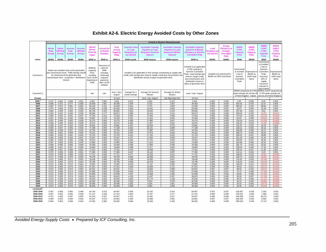
Exhibit A2-6. Electric Energy Avoided Costs by Other Zones
Winter Peak
Energy
Winter Off-Peak Energy
Summer Peak
Energy
Summer Off-Peak Energy
Annual Market
Capacity Value1
Annual Out of Market Expense
Total Annual
Capacity Value
Capacity Value at Load
Response (at any month)
Avoidable Capacity Payment at Load
Response (Summer Season)
Avoidable Capacity Payment at Load Response (Winter
Season)
Avoidable Capacity Payment at Energy
Efficiency at Summer Coincident Peak
Load Response (at any month)
Energy Efficiency at
Summer Coincident
Peak
DRIPE 0.75%
Capacity Price
DRIPE 0.75%
Capacity Price
DRIPE LIGHT 0.75%
Capacity Price
DRIPE LIGHT 0.75%
Capacity Price
Units: $/kWh $/kWh $/kWh $/kWh $/kW-yr $/kW-yr $/kW-yr $/kW-month $/kW-season $/kW-season $/kW-yr $/kWh $/kWh $/kW $/kWh $/kW $/kWh
Comment 1:
Reflects Capacity
Price resulting
from LICAP beginning in
2006
Recovery of costs for
RMR including
continuing required
payments after LICAP
initiation
Avoided Cost applicable to KW savings at
Summer Coincident Peak; load savings plus
reserve margin credit plus transmission and distribution losses to
place at generator level
Incremental to Avoided
Cost at Summer
Coincident Peak
Expressed in $/kWh at
100% load factor
Incremental to Avoided
Cost at Summer
Coincident Peak;
Assumes 10% of supply
resources transact in
spot market
Expressed in $/kWh at
100% load factor
Comment 2: info info June / July / August
Average for 1 month savings
Average for Summer Season
Average for Winter Season June / July / August
Period: 3-5 pm June, July, August Jan-May;Sept-Dec 3-5 pm2005 2 0.074 0.064 0.069 0.051 2.662 0.954 3.616 0.222 0.624 0.124 3.616 0.000 0.000 0.00 0.000 0.00 0.0002006 0.085 0.072 0.077 0.059 34.548 1.801 36.350 2.879 8.102 1.607 36.350 0.004 0.004 654.43 0.075 32.57 0.0042007 0.087 0.074 0.081 0.062 39.132 2.151 41.283 3.261 9.176 1.820 41.283 0.004 0.005 906.91 0.104 88. 0.0102008 0.074 0.060 0.072 0.050 62.436 0.199 62.635 5.203 14.641 2.903 62.635 0.007 0.007 32.87 0.004 15. 0.0022009 0.060 0.049 0.056 0.040 66.758 0.204 66.962 5.563 15.655 3.104 66.962 0.008 0.008 3 0.0 9.6 0.0012010 0.052 0.042 0.049 0.035 69.696 0.177 69.874 5.808 16.344 3.241 69.874 0.008 0.008 2 0.0 (6.8 (0.02011 0.055 0.044 0.051 0.037 72.764 0.154 72.918 6.064 17.063 3.384 72.918 0.008 0.008 174.43 0.020 (23.3 (0.02012 0.057 0.046 0.052 0.038 75.967 0.133 76.100 6.331 17.814 3.532 76.100 0.009 0.009 82.81 0.009 (39.8 (0.02013 0.057 0.046 0.053 0.039 76.270 0.000 76.270 6.356 17.885 3.547 76.270 0.009 0.009 119.16 0.014 (21.0 (0.02014 0.058 0.046 0.054 0.039 76.575 0.000 76.575 6.381 17.957 3.561 76.575 0.009 0.009 155.52 0.018 (2.3 (0.02015 0.058 0.047 0.054 0.040 76.881 0.000 76.881 6.407 18.029 3.575 76.881 0.009 0.009 191.87 0.022 16. 0.0022016 0.059 0.047 0.055 0.040 77.188 0.000 77.188 6.432 18.101 3.589 77.188 0.009 0.009 228.22 0.026 35. 0.0042017 0.060 0.049 0.057 0.042 76.704 0.000 76.704 6.392 17.987 3.567 76.704 0.009 0.009 258.99 0.030 36. 0.0042018 0.062 0.051 0.059 0.044 76.222 0.000 76.222 6.352 17.874 3.544 76.222 0.009 0.009 289.75 0.033 38. 0.0042019 0.064 0.053 0.061 0.045 75.743 0.000 75.743 6.312 17.762 3.522 75.743 0.009 0.009 320.52 0.037 39. 0.0052020 0.066 0.055 0.064 0.047 75.267 0.000 75.267 6.272 17.650 3.500 75.267 0.009 0.009 351.29 0.040 41. 0.0052021 0.066 0.055 0.065 0.048 75.613 0.000 75.613 6.301 17.731 3.516 75.613 0.009 0.009 328.09 0.037 35. 0.0042022 0.067 0.056 0.065 0.049 75.960 0.000 75.960 6.330 17.813 3.532 75.960 0.009 0.009 304.90 0.035 29.34 0.0032023 0.068 0.056 0.066 0.049 76.309 0.000 76.309 6.359 17.894 3.548 76.309 0.009 0.009 281.70 0.032 23. 0.0032024 0.068 0.057 0.067 0.050 76.660 0.000 76.660 6.388 17.977 3.565 76.660 0.009 0.009 258.50 0.030 17. 0.0022025 0.069 0.057 0.068 0.051 77.012 0.000 77.012 6.418 18.059 3.581 77.012 0.009 0.009 235.31 0.027 11. 0.0012026 0.070 0.058 0.069 0.051 77.365 0.000 77.365 6.447 18.142 3.597 77.365 0.009 0.009 212.11 0.024 5.3 0.0012027 0.070 0.059 0.069 0.052 77.721 0.000 77.721 6.477 18.225 3.614 77.721 0.009 0.009 188.91 0.022 (0.6 (0.02028 0.071 0.059 0.070 0.053 78.078 0.000 78.078 6.506 18.309 3.631 78.078 0.009 0.009 165.72 0.019 (6.6 (0.02029 0.072 0.060 0.071 0.054 78.436 0.000 78.436 6.536 18.393 3.647 78.436 0.009 0.009 142.52 0.016 (12.6 (0.02030 0.072 0.060 0.072 0.054 78.796 0.000 78.796 6.566 18.478 3.664 78.796 0.009 0.009 119.32 0.014 (18.6 (0.02031 0.072 0.060 0.072 0.054 72.952 0.000 72.952 6.079 17.107 3.392 72.952 0.008 0.008 109.42 0.012 (18.4 (0.02032 0.072 0.060 0.073 0.054 67.541 0.000 67.541 5.628 15.838 3.141 67.541 0.008 0.008 99.52 0.011 (18.2 (0.02033 0.072 0.060 0.073 0.054 62.531 0.000 62.531 5.211 14.664 2.908 62.531 0.007 0.007 89.62 0.010 (18.0 (0.02034 0.072 0.060 0.074 0.054 57.893 0.000 57.893 4.824 13.576 2.692 57.893 0.007 0.007 79.72 0.009 (17.8 (0.02035 0.072 0.059 0.074 0.053 53.599 0.000 53.599 4.467 12.569 2.492 53.599 0.006 0.006 69.82 0.008 (17.5 (0.02036 0.072 0.059 0.074 0.053 49.623 0.000 49.623 4.135 11.637 2.307 49.623 0.006 0.006 59.92 0.007 (17.3 (0.02037 0.072 0.059 0.075 0.053 45.943 0.000 45.943 3.829 10.774 2.136 45.943 0.005 0.005 50.02 0.006 (17.1 (0.02038 0.072 0.059 0.075 0.053 42.535 0.000 42.535 3.545 9.974 1.978 42.535 0.005 0.005 40.12 0.005 (16.9 (0.02039 0.072 0.059 0.076 0.053 39.380 0.000 39.380 3.282 9.235 1.831 39.380 0.004 0.004 30.22 0.003 (16.7 (0.02040 0.072 0.059 0.076 0.053 36.459 0.000 36.459 3.038 8.550 1.695 36.459 0.004 0.004 20.32 0.002 (16.5 (0.0
Levelized3: 2005-2040 0.067 0.056 0.065 0.048 64.742 0.215 64.957 5.395 15.182 3.010 64.957 0.007 0.007 220.657 0.025 7.20 0.02006-2040 0.067 0.055 0.065 0.048 67.237 0.186 67.422 5.603 15.767 3.127 67.422 0.008 0.008 229.525 0.026 7.48 0.02006-2010 0.072 0.060 0.067 0.050 54.120 0.927 55.047 4.510 12.691 2.517 55.047 0.006 0.006 448.938 0.051 28.472 0.0032006-2015 0.065 0.053 0.060 0.044 64.347 0.515 64.862 5.362 15.089 2.992 64.862 0.007 0.007 304.283 0.035 8.063 0.0012006-2020 0.064 0.052 0.060 0.044 67.922 0.360 68.282 5.660 15.928 3.158 68.282 0.008 0.008 299.546 0.034 17.117 0.002
DRIPE measured at 0.75% peak savings are across all
of New England. Values
DRIPE LIGHT measured at 0.75% peak savings are
across all of New England.
Central & Western Massachusetts
Values are avoided costs at the generation plus transmission level. DSM savings should
be measured at the generator plus transmission level. (Load plus + distribution
losses)
Avoided Cost applicable to KW savings contributing as supply side credit; load savings plus reserve margin credit plus transmission and
distribution losses to place at generator level
Avoided cost expressed in $/kWh at 100% load factor
6028
57.68 41 266.06 30 7) 01)
5) 03)4) 05)8) 02)
3) 00)43187226803434
34353555) 00)5) 01)4) 01)4) 02)3) 02)2) 02)1) 02)0) 02)9) 02)8) 02)7) 02)6) 02)5) 02)4) 02)
0 019 01
Avoided Energy-Supply Costs • Prepared by ICF Consulting, Inc.
205
Avoided Energy-Supply Costs • Prepared by ICF Consulting, Inc.
206
Appendix Three: Sources
Algonquin Gas Transmission Co., Tariff. http://infopost.link.duke-energy.com/InfoPost/default.asp?pipe=AG
Alternatives to Velco’s Northwest Vermont Reliability Project, 29 January, 2003.
Cross Sound Cable Company, LLC – Notice to Market Participants, July 2004.
Cross Sound Cable Company, LLC – NY, Connecticut Resolve Transmission Dispute, June 24, 2004.
DOE Annual Energy Outlook 2005, January 2005, Table 66.
Energy Information Administration (EIA) Electric Power Monthly, Average Retail Price of Electricity to Ultimate Customers by End-Use Sector, by State, Year-to-Date through May 2005 and 2004, August 8, 2005.
EIA, Natural Gas, www.eia.doe.gov/oil gas/natural gas/info glance/natural gas.html. Various historical statistics on gas consumption.
EIA Form 826, Monthly Electric Sales and Revenue Report with State Distributions Report.
EIA, Short Term Energy Outlook, 2005.
FERC Form 1’s for Western Massachusetts Electric Company, Massachusetts Electric Company, Boston Edison, Commonwealth Electric, Fitchburg Gas & Electric Light Company and Cambridge Electric Light Company, 2002-2004.
FERC Form 714 – Annual Electric Control and Planning Area Report, http://www.ferc.gov/docs-filing/eforms/form-714/data.asp.
Filing 2004-12-16 Integrated LICAP Impact Model Multi-year Mods (Excel Spreadsheet).
Gas Daily. Various Issues.
ISO New England’s 2005-2014 Forecast Report of Capacity Energy Load and Transmission, April 2005.
ISO New England’s RMR Agreements Summary with Fixed Costs, July 27, 2005.
ISO New England’s 2004 Annual Markets Report, July 15, 2005.
Avoided Energy-Supply Costs • Prepared by ICF Consulting, Inc.
207
ISO New England’s 2004 Summary Report – Regional Transmission Expansion Plan, October 21, 2004.
ISO New England/NEPOOL Demand Response Working Group Meeting, July 6, 2005.
ISO New England’s Final Report on Evaluation and Selection of Resources in SWCT RFP for Emergency Capability 2004-2008.
Jefferies Electric Utilities – Industry Update – March 18, 2005. LICAP Privateers: Pirates or New England Patriots?
July ’05 ISO New England Project Listing Update (FINAL), July 29, 2005.
La Capra Associates – CT Electric Supply and Demand Near Term Requirements for Reliability and Mitigation of FMCCs (Preliminary Assessment), August 30, 2005.
Nepool Reliability Committee Memo, May 24, 2004.
Northeast Gas Association. Industry Information. www.northeastgas.org
Public_2005-05-18 LICAP Model Clearing Price and Cost Model (Excel Spreadsheet).
Tennessee Gas Pipeline. Tariff. http://tebb.epenergy.com/ebb/ebbmain.asp?sPipelineCode=TGP
Texas Eastern Transmission. Tariff. http://infopost.link.duke-energy.com/InfoPost/default.asp?pipe=TE
The Connecticut Energy Board – Connecticut’s Electric Supply and Demand – Near Term Requirements for Reliability and Mitigation of Federally Mandated Congestion Charges, September 2, 2005.
United States of America before the Federal Energy Regulatory Commission – Prepared Direct Testimony of Steven E. Stoft on behalf of ISO New England Inc.
United States of America before the Federal Energy Regulatory Commission – Rebuttal Testimony of Steven Stoft. Docket No. ER03-563-030. February 10, 2005.
United States of America before the Federal Energy Regulatory Commission – Prepared Direct Testimony of John J. Reed on behalf of ISO New England Inc.
United States of America before the Federal Energy Regulatory Commission – Prepared Rebuttal Testimony of John J. Reed. Docket No. ER03-563-030. February 10, 2005.