Embed Size (px)
Citation preview
Avoided Energy Supply Costs in New England: 2007 FINAL REPORT FINAL - August 10, 2007
AUTHORS
Rick Hornby, Dr. Carl V. Swanson, Michael Drunsic, Dr. David E. White, Paul Chernick, Bruce Biewald, and Jennifer Kallay PREPARED FOR
Avoided-Energy-Supply-Component (AESC) Study Group
Table of Contents
1. Executive Summary................................................................................................. 1-1 A. Background to Report .................................................................................... 1-1 B. Organization of Report .................................................................................. 1-2 C. Results and Comparison to 2005 AESC ........................................................ 1-2
2. Natural Gas Price Forecast ..................................................................................... 2-1 A. Overview of New England Gas Market......................................................... 2-1 B. Forecast Commodity Price of Gas ................................................................. 2-3 C. Forecast of High and Low Gas Prices at the Henry Hub............................... 2-9 D. Representation of Volatility in Gas Commodity Prices............................... 2-10 E. Forecast of Price for Electric Generation in New England.......................... 2-12 F. Impact of New Regional Supplies on Regional Price of Natural Gas ......... 2-15 G. Forecast of Price for Retail Sectors ............................................................. 2-19
3. Crude Oil Price Forecast......................................................................................... 3-1 A. Methodology & Assumptions ........................................................................ 3-1 B. Results............................................................................................................ 3-3
4. Forecasts of Other Fuel Prices................................................................................ 4-1 A. Methodology & Assumptions ........................................................................ 4-1 B. Results............................................................................................................ 4-6
5. Electric Energy Price Forecast ............................................................................... 5-1 A. Overview........................................................................................................ 5-1 B. Zonal Locational Marginal Price-Forecasting Model.................................... 5-1 C. Input Assumptions Used to Develop the Electric Energy Price Forecast...... 5-3 D. Results.......................................................................................................... 5-21 E. Transmission Energy Losses........................................................................ 5-23 F. Key Sources of Uncertainty in Forecast Energy Prices ............................... 5-25
6. Avoided Electricity Supply Costs ........................................................................... 6-1 A. Avoided Cost of Compliance with RPS......................................................... 6-2 B. Avoided Capacity Costs................................................................................. 6-3 C. Adjustment of Capacity Costs for Losses on ISO-Administered Pool
Transmission Facilities ................................................................................ 6-11 D. Retail Adder ................................................................................................. 6-12 E. Demand-Reduction-Induced Price Effects (DRIPE) for Energy and Capacity.. 6-13
7. Environmental Effects ............................................................................................. 7-1 A. Physical Environmental Benefits from Energy Efficiency and Demand
Reductions...................................................................................................... 7-1 B. Monetized Emission Values .......................................................................... 7-6
Appendix A – Common Modeling Assumptions
Appendix B – Forecasts of Monthly Natural Gas Prices
Appendix C – Detailed Input Assumptions for Electric Energy Price Forecast
Appendix D – Usage Guide for Avoided Energy Supply Costs
Appendix E – Avoided Electric Costs
Synapse Energy Economics – 2007 AESC 1-1
1. Executive Summary
A. Background to Report This 2007 Avoided-Energy-Supply-Component (AESC) report provides projections of marginal energy supply costs which will be avoided due to savings in electricity, natural gas, and other fuels resulting from energy efficiency programs offered to customers throughout New England. These projections were developed in order to support energy efficiency program decision-making and regulatory filings during 2008 and 2009. The program administrators will use these projections in their efficiency program decision-making and regulatory filings in 2008 and 2009.
The 2007 AESC Study updates the 2005 AESC Study to reflect current market conditions and cost projections. The report provides detailed projections for an initial fifteen year period beginning in 2007 and escalation rates for another fifteen years from 2022 through 2037. All values are reported in 2007$ unless noted otherwise. The 2007 AESC Study was sponsored by a group of electric utilities, gas utilities and other efficiency program administrators (collectively, “program administrators”). The sponsors, along with non-utility parties and their consultants, formed a 2007 AESC Study Group to oversee the design and execution of the report. The 2007 AESC sponsors include Berkshire Gas Company, KeySpan Energy Delivery New England (Boston Gas Company, Essex Gas Company, Colonial Gas Company, and EnergyNorth Natural Gas, Inc.), Cape Light Compact, National Grid USA, New England Gas Company, NSTAR Electric & Gas Company, New Hampshire Electric Co-op, Bay State Gas and Northern Utilities, Northeast Utilities (Connecticut Light and Power, Western Massachusetts Electric Company, Public Service Company of New Hampshire, and Yankee Gas), Unitil (Fitchburg Gas and Electric Light Company and Unitil Energy Systems, Inc.), United Illuminating, Southern Connecticut Gas and Connecticut Natural Gas, the State of Maine, and the State of Vermont. The following agencies or organizations are represented in the Study Group: Connecticut Energy Conservation Management Board, Massachusetts Department of Public Utilities, Massachusetts Division of Energy Resources, Massachusetts Low-Income Energy Affordability Network (LEAN) and other Non-Utility Parties, New Hampshire Public Utilities Commission, and Rhode Island Division of Public Utilities and Carriers.
The 2007 AESC Study Group specified the scope of work, selected the contractor, and monitored progress of the study. The report was prepared by a project team consisting of contractors from Synapse Energy Economics (Synapse), Swanson Energy Group and Resource Insight (Synapse project team). Carl Swanson led the analysis of avoided natural gas costs and David White was lead investigator on projections of prices of oil and other fuels. Michael Drunsic was responsible for projecting electricity prices with advice from Bruce Biewald, Paul Chernick and David White. Doug Hurley provided advice on the structure and operation of the New England market, including ICAP and LICAP issues.
Synapse Energy Economics – 2007 AESC 1-2
Paul Chernick developed zonal avoided electric costs by costing period, including analyses of DRIPE. Bruce Biewald, Paul Chernick, and Lucy Johnston developed estimates of environmental externalities. Jennifer Kallay provided research and analytic support including data collection, literature searches, spreadsheet analyses, documentation, and drafting. Rick Hornby served as project manager and editor. The Synapse project team presented its analyses and projections to the 2007 AESC Study Group in nine substantive analyses, each of which was reviewed in a conference call.
B. Organization of Report The report provides detailed projections of marginal energy supply costs for an initial fifteen year period beginning in 2007 and escalation rates for another fifteen years from 2022 through 2037. All values are reported in 2007$ unless noted otherwise.
The report is organized as follows: • Chapter 2 - projection of natural gas prices for electric generation as well as a
projection of avoided natural gas costs by retail end-use sector.
• Chapter 3 - projection of crude oil prices.
• Chapter 4 - projection of fuel prices by retail end-use sector.
• Chapter 5 - projection of electric energy prices and a description of the modeling methodology and assumptions.
• Chapter 6 - projection of avoided electricity costs and a description of the underlying assumptions.
• Chapter 7 - projection of environmental effects and environmental externalities.
• Appendix A – derivation of common modeling assumptions.
• Appendix B – avoided gas costs in 2007$ and nominal$.
• Appendix C – detailed input assumptions for electric energy price forecasts.
• Appendix D – usage guide for avoided electricity supply costs.
• Appendix E – avoided electricity supply costs in 2007$ and nominal$.
C. Results and Comparison to 2005 AESC Avoided Costs of Natural Gas to Retail Customers
The 2007 AESC projections of marginal natural gas supply costs to retail customers over the next fifteen years range from $8.00 to $12.00 per dekatherm (DT) (2007$). The 2007 AESC projections are generally higher than the 2005 AESC projections, shown in
Synapse Energy Economics – 2007 AESC 1-3
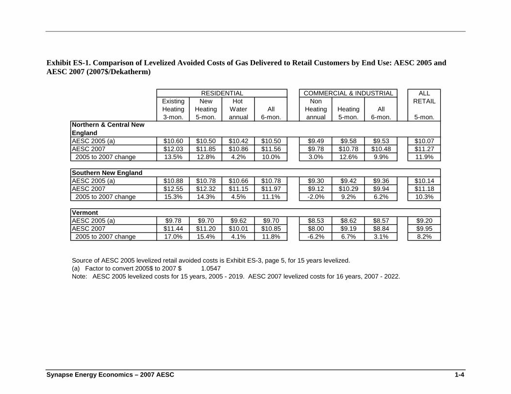
Exhibit ES-11. Exceptions to these generally higher results occur in commercial/industrial non-heating applications in Southern New England and Vermont.
The differences between the 2007 AESC projections and the 2005 AESC projections are primarily due to a higher projection for natural gas prices, discussed further below. In addition, AESC 2007 projects a higher avoided retail margin for residential applications, especially in Northern & Central New England, compared with AESC 2005. The lower projection of avoided cost in AESC 2007 for commercial and industrial non-heating, applications in Southern New England is primarily due to a lower projection of avoided retail margin for that application. The AESC 2007 projection is based upon a volume weighted average of the estimated avoided margins for the industrial and the commercial sectors respectively, while the AESC 2005 projection is based only on the estimated avoided commercial retail margin. This difference in methodology also appears to explain the lower AESC 2007 estimates of commercial and industrial non-heating avoided costs in Vermont.
1 2007 AESC values levelized for 15 years (2008 - 2022) at discount rate of 2.22%. 2005 AESC values
levelized for 15 years (2006 - 2020) at discount rate of 2.03%.
Synapse Energy Economics – 2007 AESC 1-4
Exhibit ES-1. Comparison of Levelized Avoided Costs of Gas Delivered to Retail Customers by End Use: AESC 2005 and AESC 2007 (2007$/Dekatherm)
ALLExisting New Hot Non RETAILHeating Heating Water All Heating Heating All3-mon. 5-mon. annual 6-mon. annual 5-mon. 6-mon. 5-mon.
Northern & Central New EnglandAESC 2005 (a) $10.60 $10.50 $10.42 $10.50 $9.49 $9.58 $9.53 $10.07AESC 2007 $12.03 $11.85 $10.86 $11.56 $9.78 $10.78 $10.48 $11.27 2005 to 2007 change 13.5% 12.8% 4.2% 10.0% 3.0% 12.6% 9.9% 11.9%
Southern New EnglandAESC 2005 (a) $10.88 $10.78 $10.66 $10.78 $9.30 $9.42 $9.36 $10.14AESC 2007 $12.55 $12.32 $11.15 $11.97 $9.12 $10.29 $9.94 $11.18 2005 to 2007 change 15.3% 14.3% 4.5% 11.1% -2.0% 9.2% 6.2% 10.3%
VermontAESC 2005 (a) $9.78 $9.70 $9.62 $9.70 $8.53 $8.62 $8.57 $9.20AESC 2007 $11.44 $11.20 $10.01 $10.85 $8.00 $9.19 $8.84 $9.95 2005 to 2007 change 17.0% 15.4% 4.1% 11.8% -6.2% 6.7% 3.1% 8.2%
Source of AESC 2005 levelized retail avoided costs is Exhibit ES-3, page 5, for 15 years levelized.(a) Factor to convert 2005$ to 2007 $ 1.0547Note: AESC 2005 levelized costs for 15 years, 2005 - 2019. AESC 2007 levelized costs for 16 years, 2007 - 2022.
RESIDENTIAL COMMERCIAL & INDUSTRIAL
Synapse Energy Economics – 2007 AESC 1-5
Avoided Costs of Electricity to Retail Customers
The 2007 AESC projections of marginal electric energy and capacity costs to retail customers are substantially higher than those in the 2005 AESC Study. The 15 year levelized projections2 of marginal electric energy costs from the 2005 and 2007 AESC studies are shown in Exhibit ES-2.
2 2007 AESC values and AESC 2005 values levelized for 15 years (2008 - 2022) at discount rate of
2.22%.
Synapse Energy Economics – 2007 AESC 1-6
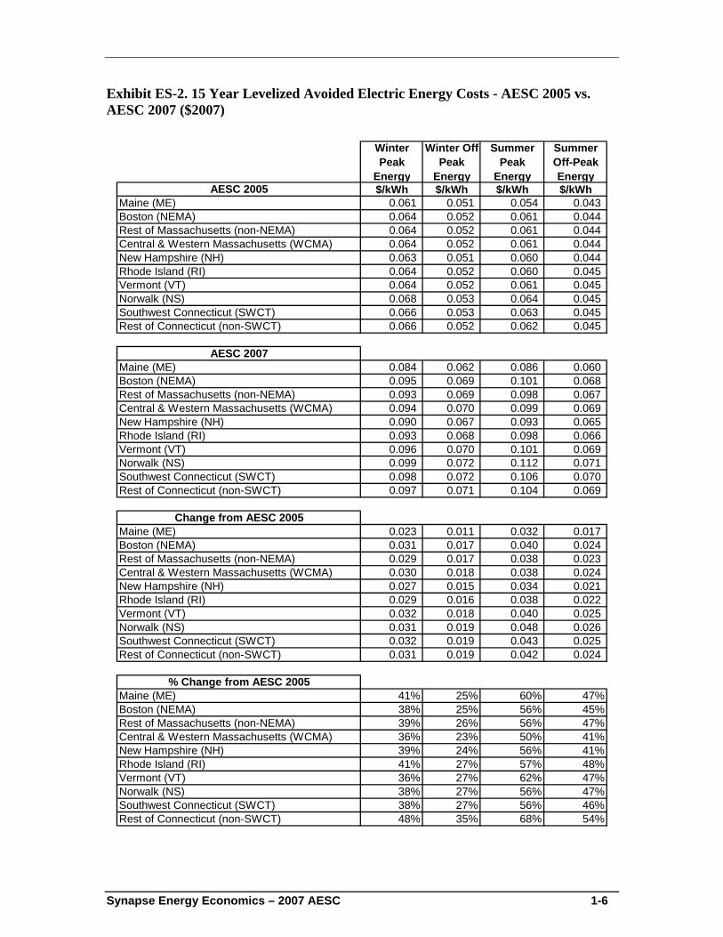
Exhibit ES-2. 15 Year Levelized Avoided Electric Energy Costs - AESC 2005 vs. AESC 2007 ($2007)
Winter Peak
Energy
Winter Off-Peak
Energy
Summer Peak
Energy
Summer Off-Peak Energy
AESC 2005 $/kWh $/kWh $/kWh $/kWhMaine (ME) 0.061 0.051 0.054 0.043 Boston (NEMA) 0.064 0.052 0.061 0.044 Rest of Massachusetts (non-NEMA) 0.064 0.052 0.061 0.044 Central & Western Massachusetts (WCMA) 0.064 0.052 0.061 0.044 New Hampshire (NH) 0.063 0.051 0.060 0.044 Rhode Island (RI) 0.064 0.052 0.060 0.045 Vermont (VT) 0.064 0.052 0.061 0.045 Norwalk (NS) 0.068 0.053 0.064 0.045 Southwest Connecticut (SWCT) 0.066 0.053 0.063 0.045 Rest of Connecticut (non-SWCT) 0.066 0.052 0.062 0.045
AESC 2007Maine (ME) 0.084 0.062 0.086 0.060 Boston (NEMA) 0.095 0.069 0.101 0.068 Rest of Massachusetts (non-NEMA) 0.093 0.069 0.098 0.067 Central & Western Massachusetts (WCMA) 0.094 0.070 0.099 0.069 New Hampshire (NH) 0.090 0.067 0.093 0.065 Rhode Island (RI) 0.093 0.068 0.098 0.066 Vermont (VT) 0.096 0.070 0.101 0.069 Norwalk (NS) 0.099 0.072 0.112 0.071 Southwest Connecticut (SWCT) 0.098 0.072 0.106 0.070 Rest of Connecticut (non-SWCT) 0.097 0.071 0.104 0.069
Change from AESC 2005Maine (ME) 0.023 0.011 0.032 0.017 Boston (NEMA) 0.031 0.017 0.040 0.024 Rest of Massachusetts (non-NEMA) 0.029 0.017 0.038 0.023 Central & Western Massachusetts (WCMA) 0.030 0.018 0.038 0.024 New Hampshire (NH) 0.027 0.015 0.034 0.021 Rhode Island (RI) 0.029 0.016 0.038 0.022 Vermont (VT) 0.032 0.018 0.040 0.025 Norwalk (NS) 0.031 0.019 0.048 0.026 Southwest Connecticut (SWCT) 0.032 0.019 0.043 0.025 Rest of Connecticut (non-SWCT) 0.031 0.019 0.042 0.024
% Change from AESC 2005Maine (ME) 41% 25% 60% 47%Boston (NEMA) 38% 25% 56% 45%Rest of Massachusetts (non-NEMA) 39% 26% 56% 47%Central & Western Massachusetts (WCMA) 36% 23% 50% 41%New Hampshire (NH) 39% 24% 56% 41%Rhode Island (RI) 41% 27% 57% 48%Vermont (VT) 36% 27% 62% 47%Norwalk (NS) 38% 27% 56% 47%Southwest Connecticut (SWCT) 38% 27% 56% 46%Rest of Connecticut (non-SWCT) 48% 35% 68% 54%
Synapse Energy Economics – 2007 AESC 1-7
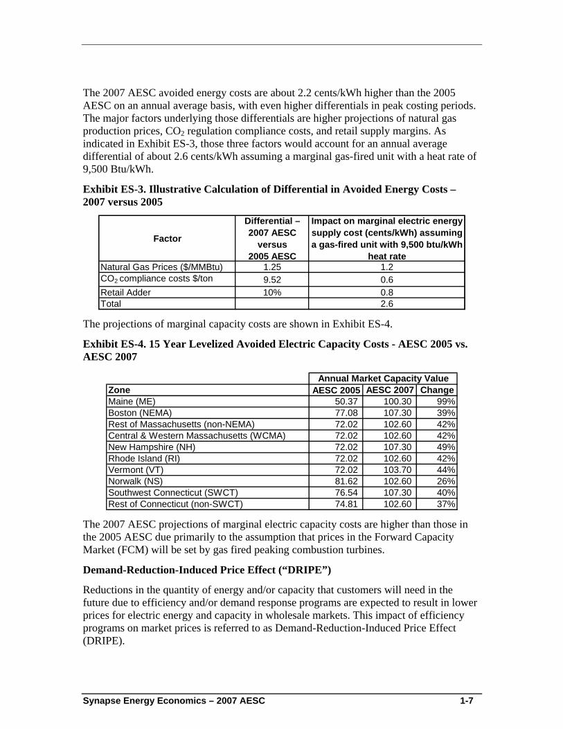
The 2007 AESC avoided energy costs are about 2.2 cents/kWh higher than the 2005 AESC on an annual average basis, with even higher differentials in peak costing periods. The major factors underlying those differentials are higher projections of natural gas production prices, CO2 regulation compliance costs, and retail supply margins. As indicated in Exhibit ES-3, those three factors would account for an annual average differential of about 2.6 cents/kWh assuming a marginal gas-fired unit with a heat rate of 9,500 Btu/kWh.
Exhibit ES-3. Illustrative Calculation of Differential in Avoided Energy Costs – 2007 versus 2005
Factor
Differential – 2007 AESC
versus 2005 AESC
Impact on marginal electric energy supply cost (cents/kWh) assuming a gas-fired unit with 9,500 btu/kWh
heat rateNatural Gas Prices ($/MMBtu) 1.25 1.2CO2 compliance costs $/ton 9.52 0.6Retail Adder 10% 0.8Total 2.6
The projections of marginal capacity costs are shown in Exhibit ES-4.
Exhibit ES-4. 15 Year Levelized Avoided Electric Capacity Costs - AESC 2005 vs. AESC 2007
Zone AESC 2005 AESC 2007 ChangeMaine (ME) 50.37 100.30 99%Boston (NEMA) 77.08 107.30 39%Rest of Massachusetts (non-NEMA) 72.02 102.60 42%Central & Western Massachusetts (WCMA) 72.02 102.60 42%New Hampshire (NH) 72.02 107.30 49%Rhode Island (RI) 72.02 102.60 42%Vermont (VT) 72.02 103.70 44%Norwalk (NS) 81.62 102.60 26%Southwest Connecticut (SWCT) 76.54 107.30 40%Rest of Connecticut (non-SWCT) 74.81 102.60 37%
Annual Market Capacity Value
The 2007 AESC projections of marginal electric capacity costs are higher than those in the 2005 AESC due primarily to the assumption that prices in the Forward Capacity Market (FCM) will be set by gas fired peaking combustion turbines.
Demand-Reduction-Induced Price Effect (“DRIPE”)
Reductions in the quantity of energy and/or capacity that customers will need in the future due to efficiency and/or demand response programs are expected to result in lower prices for electric energy and capacity in wholesale markets. This impact of efficiency programs on market prices is referred to as Demand-Reduction-Induced Price Effect (DRIPE).
Synapse Energy Economics – 2007 AESC 1-8
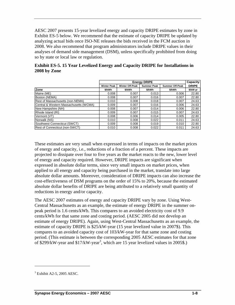
AESC 2007 presents 15-year levelized energy and capacity DRIPE estimates by zone in Exhibit ES-5 below. We recommend that the estimate of capacity DRIPE be updated by analyzing actual bids once ISO-NE releases the bids received in the FCM auction in 2008. We also recommend that program administrators include DRIPE values in their analyses of demand side management (DSM), unless specifically prohibited from doing so by state or local law or regulation.
Exhibit ES-5. 15 Year Levelized Energy and Capacity DRIPE for Installations in 2008 by Zone
Winter Peak Winter Off-Peak Summer Peak Summer Off-PeakZone $/kWh $/kWh $/kWh $/kWh $/kW-yrMaine (ME) 0.008 0.007 0.013 0.006 22.80 Boston (NEMA) 0.008 0.007 0.016 0.007 22.80 Rest of Massachusetts (non-NEMA) 0.010 0.008 0.018 0.007 24.63 Central & Western Massachusetts (WCMA) 0.009 0.007 0.016 0.006 24.63 New Hampshire (NH) 0.008 0.007 0.014 0.006 22.80 Rhode Island (RI) 0.009 0.007 0.015 0.007 24.63 Vermont (VT) 0.008 0.006 0.014 0.005 22.80 Norwalk (NS) 0.010 0.008 0.022 0.011 24.63 Southwest Connecticut (SWCT) 0.009 0.008 0.019 0.010 22.80 Rest of Connecticut (non-SWCT) 0.010 0.008 0.022 0.011 24.63
Energy DRIPE Capacity DRIPE
These estimates are very small when expressed in terms of impacts on the market prices of energy and capacity, i.e., reductions of a fraction of a percent. These impacts are projected to dissipate over four to five years as the market reacts to the new, lower level of energy and capacity required. However, DRIPE impacts are significant when expressed in absolute dollar terms, since very small impacts on market prices, when applied to all energy and capacity being purchased in the market, translate into large absolute dollar amounts. Moreover, consideration of DRIPE impacts can also increase the cost-effectiveness of DSM programs on the order of 15% to 20%, because the estimated absolute dollar benefits of DRIPE are being attributed to a relatively small quantity of reductions in energy and/or capacity.
The AESC 2007 estimates of energy and capacity DRIPE vary by zone. Using West-Central Massachusetts as an example, the estimate of energy DRIPE in the summer on-peak period is 1.6 cents/kWh. This compares to an avoided electricity cost of 9.9 cents/kWh for that same zone and costing period. (AESC 2005 did not develop an estimate of energy DRIPE). Again, using West-Central Massachusetts as an example, the estimate of capacity DRIPE is $25/kW-year (15 year levelized value in 2007$). This compares to an avoided capacity cost of 103/kW-year for that same zone and costing period. (This estimate is between the corresponding 2005 AESC estimates for that zone of $299/kW-year and $17/kW-year3, which are 15 year levelized values in 2005$.)
3 Exhibit A2-5, 2005 AESC.
Synapse Energy Economics – 2007 AESC 1-9
CO2 Externality
Externalities are impacts from the production of a good or service that are neither reflected in the price of that good or service nor considered in the decision to provide that good or service. There are many externalities associated with the production of electricity, including the adverse impacts of emissions of SO2, mercury, particulates, NOx and CO2. However, the magnitude of most of those externalities has been reduced over time, as regulations limiting emission levels have forced suppliers and buyers to consider at least a portion of their adverse impacts in their production and use decisions. In other words, a portion of the costs of the adverse impact of most of these externalities has already been “internalized” in the price of electricity.
AESC 2007 identifies the impacts of carbon dioxide as the dominant externality associated with marginal electricity generation in New England over the study period for two main reasons. First, policy makers are just starting to develop and implement regulations that will “internalize” the costs associated with the impacts of carbon dioxide from electricity production and other energy uses. The Regional Greenhouse Gas Initiative and anticipated future federal CO2 regulations will internalize a portion of the "greenhouse gas externality," but AESC 2007 projects that the externality value of CO2 will still be high even with those regulations. Second, New England avoided electric energy costs over the study period are likely to be dominated by natural gas-fired generation, which has minimal emissions of SO2, mercury, particulates and NOX, but substantial emissions of CO2.
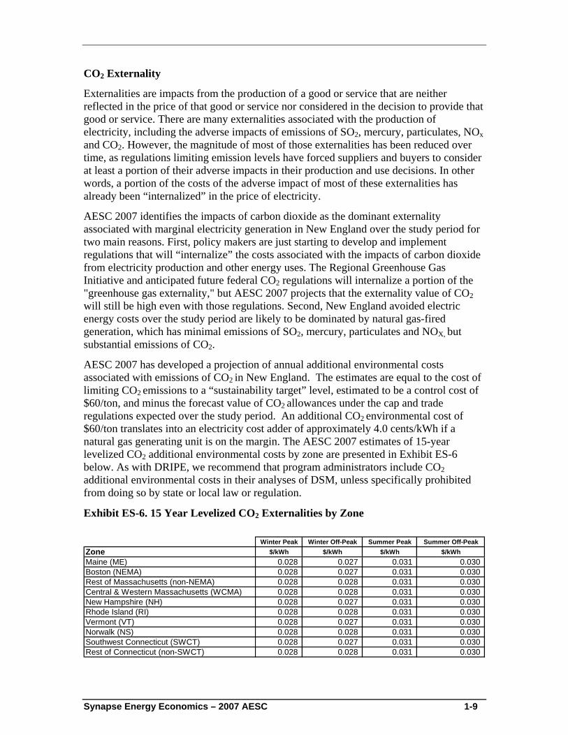
AESC 2007 has developed a projection of annual additional environmental costs associated with emissions of CO2 in New England. The estimates are equal to the cost of limiting CO2 emissions to a “sustainability target” level, estimated to be a control cost of $60/ton, and minus the forecast value of CO2 allowances under the cap and trade regulations expected over the study period. An additional CO2 environmental cost of $60/ton translates into an electricity cost adder of approximately 4.0 cents/kWh if a natural gas generating unit is on the margin. The AESC 2007 estimates of 15-year levelized CO2 additional environmental costs by zone are presented in Exhibit ES-6 below. As with DRIPE, we recommend that program administrators include CO2 additional environmental costs in their analyses of DSM, unless specifically prohibited from doing so by state or local law or regulation.
Exhibit ES-6. 15 Year Levelized CO2 Externalities by Zone
Winter Peak Winter Off-Peak Summer Peak Summer Off-PeakZone $/kWh $/kWh $/kWh $/kWhMaine (ME) 0.028 0.027 0.031 0.030 Boston (NEMA) 0.028 0.027 0.031 0.030 Rest of Massachusetts (non-NEMA) 0.028 0.028 0.031 0.030 Central & Western Massachusetts (WCMA) 0.028 0.028 0.031 0.030 New Hampshire (NH) 0.028 0.027 0.031 0.030 Rhode Island (RI) 0.028 0.028 0.031 0.030 Vermont (VT) 0.028 0.027 0.031 0.030 Norwalk (NS) 0.028 0.028 0.031 0.030 Southwest Connecticut (SWCT) 0.028 0.027 0.031 0.030 Rest of Connecticut (non-SWCT) 0.028 0.028 0.031 0.030
Synapse Energy Economics – 2007 AESC 2-1
2. Natural Gas Price Forecast This Chapter provides a projection of natural gas prices for electric generation as well as a projection of avoided natural gas costs by retail end-use sector.
A. Overview of New England Gas Market Natural gas arrived later in New England than in much of the rest of America because of its distance from the major supplies of natural gas in the Southwest. Now, however, natural gas accounts for approximately 23 percent of New England energy consumption, which is the same fraction of energy consumption as in the United States as a whole. Gas consumption has been and is expected to continue to grow in New England with electricity generation the most rapidly growing sector. Most of the gas purchased by consumers in New England is delivered by local distribution companies (LDCs), but some is delivered directly by pipelines, usually to electric generation facilities.
Because of the large seasonal temperature changes in New England and the amount of heating load, natural gas use is seasonal. On average, about twice as much gas is used in January than in the summer months. However, much of the summer natural gas consumption is for electricity generation. Since generators often receive gas directly from pipelines, the LDCs have a much greater swing of gas load; an LDC’s January gas load can be five times its summer load. Because of these large swings in gas load, LDCs must have gas stored in the summer to serve customer gas requirements in the winter. This stored gas is mostly stored in underground facilities, many of which are depleted natural gas producing fields. Most of the underground storage facilities that serve the New England LDCs are located in Pennsylvania, although storage facilities in New York, Michigan, and Ontario are also used. Since these underground storage facilities are relatively far from New England, liquefied natural gas (LNG) and propane stored in New England are used to meet the peak customer requirement on the colder days of the winter.
Originally the natural gas delivered in New England came from the supply areas of Appalachia or the Southwest. New England’s natural gas supply has diversified; gas also now comes from western Canada, from Nova Scotia, and by ship as LNG from Trinidad and Tobago, Nigeria, Algeria, and other LNG exporting countries.
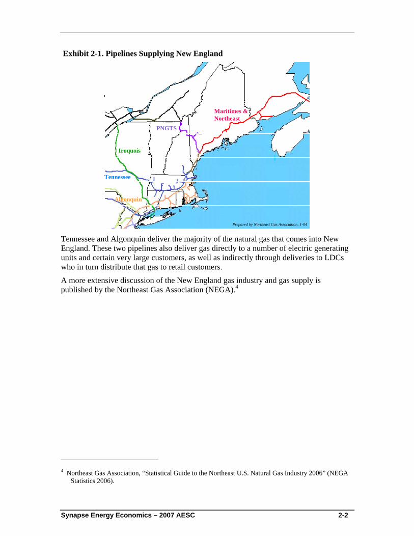
The physical system through which gas is delivered to and within the New England region, excluding Vermont, currently consists of five pipelines and one liquefied natural gas terminal. The pipelines are Tennessee, Algonquin, Maritimes & Northeast, Portland Natural Gas, and Iroquois, and the LNG terminal is owned and operated by Distrigas. A map of these five pipelines is shown in Exhibit 2-1 below. Distrigas receives LNG by tanker in Boston Harbor and delivers that supply as gas into Algonquin, the KeySpan system, the Mystic Electric Generating Station, and as LNG by truck to local distribution company (LDC) storage tanks throughout the region. The one LDC serving northern Vermont receives its gas from TransCanada Pipelines at Highgate Springs on the border with Canada.
Synapse Energy Economics – 2007 AESC 2-2
Exhibit 2-1. Pipelines Supplying New England
Iroquois
Tennessee
Algonquin
Maritimes &Northeast
PNGTS
Prepared by Northeast Gas Association, 1-04 Tennessee and Algonquin deliver the majority of the natural gas that comes into New England. These two pipelines also deliver gas directly to a number of electric generating units and certain very large customers, as well as indirectly through deliveries to LDCs who in turn distribute that gas to retail customers.
A more extensive discussion of the New England gas industry and gas supply is published by the Northeast Gas Association (NEGA).4
4 Northeast Gas Association, “Statistical Guide to the Northeast U.S. Natural Gas Industry 2006” (NEGA
Statistics 2006).
Synapse Energy Economics – 2007 AESC 2-3
B. Forecast Commodity Price of Gas
i. Development of Henry Hub Natural Gas Price Forecast
The forecasted commodity price of gas in New England begins with a forecast of the price of gas at the Henry Hub, the most relevant pricing point for US gas supply costs. Henry Hub natural gas prices make a good starting point for the forecast for numerous reasons, including: the North American natural gas market is highly integrated, the Henry Hub is located in the US Gulf Coast area which is the dominant producing region of the United States, the Henry Hub is the most liquid trading hub with the longest history of public trading on the New York Mercantile Exchange (“NYMEX”), and market prices of gas produced in other regions of the United States and Canada reflect Henry Hub prices with an adjustment for their location – referred to as a basis differential. A basis differential is defined as the natural gas price in a market location minus the gas price at the Henry Hub.
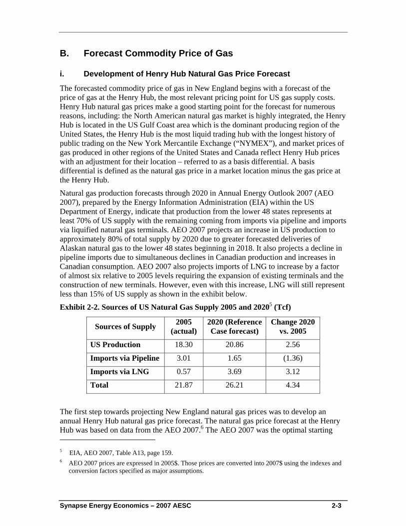
Natural gas production forecasts through 2020 in Annual Energy Outlook 2007 (AEO 2007), prepared by the Energy Information Administration (EIA) within the US Department of Energy, indicate that production from the lower 48 states represents at least 70% of US supply with the remaining coming from imports via pipeline and imports via liquified natural gas terminals. AEO 2007 projects an increase in US production to approximately 80% of total supply by 2020 due to greater forecasted deliveries of Alaskan natural gas to the lower 48 states beginning in 2018. It also projects a decline in pipeline imports due to simultaneous declines in Canadian production and increases in Canadian consumption. AEO 2007 also projects imports of LNG to increase by a factor of almost six relative to 2005 levels requiring the expansion of existing terminals and the construction of new terminals. However, even with this increase, LNG will still represent less than 15% of US supply as shown in the exhibit below.
Exhibit 2-2. Sources of US Natural Gas Supply 2005 and 20205 (Tcf)
Sources of Supply 2005 (actual)
2020 (Reference Case forecast)
Change 2020 vs. 2005
US Production 18.30 20.86 2.56
Imports via Pipeline 3.01 1.65 (1.36)
Imports via LNG 0.57 3.69 3.12
Total 21.87 26.21 4.34
The first step towards projecting New England natural gas prices was to develop an annual Henry Hub natural gas price forecast. The natural gas price forecast at the Henry Hub was based on data from the AEO 2007.6 The AEO 2007 was the optimal starting 5 EIA, AEO 2007, Table A13, page 159. 6 AEO 2007 prices are expressed in 2005$. Those prices are converted into 2007$ using the indexes and
conversion factors specified as major assumptions.
Synapse Energy Economics – 2007 AESC 2-4
point because it is public, transparent, and incorporates the long-term feedback mechanisms of energy prices upon supply, demand, and competition among fuels. AEO 2007 is comprised of 34 different forecast cases, each incorporating different assumptions.7 The most likely case is called a Reference Case. The Reference Case assumes US economic growth of 2.9% per year and oil and gas prices that decline from current levels and then begin a slow rise. By 2030, the AEO 2007 expects the Reference Case average crude oil prices to be about $59.00 per barrel and US wellhead natural gas prices to be $5.80 per Mcf in 2007 dollars.
A review of the Henry Hub natural gas prices in AEO 2007 found that none of the AEO forecasts of Henry Hub gas prices over the long-term were supportable. A major source of disagreement with the AEO 2007 forecasting was with the EIA’s assumptions about technological progress in oil and gas finding. As indicated in Exhibit 2-3, the AEO Reference Case assumes that, relative to actual experience over the past ten years,
• the success rate of oil and gas drilling will improve at a slower pace,
• the finding rates for gas will improve at a faster pace, and
• the costs of drilling wells will decline at a faster rate.
For the reasons presented below, we agree with the EIA’s projections that the success rate of drilling will improve at a slower pace but we disagree with their projected improvements in finding rates and drilling costs.
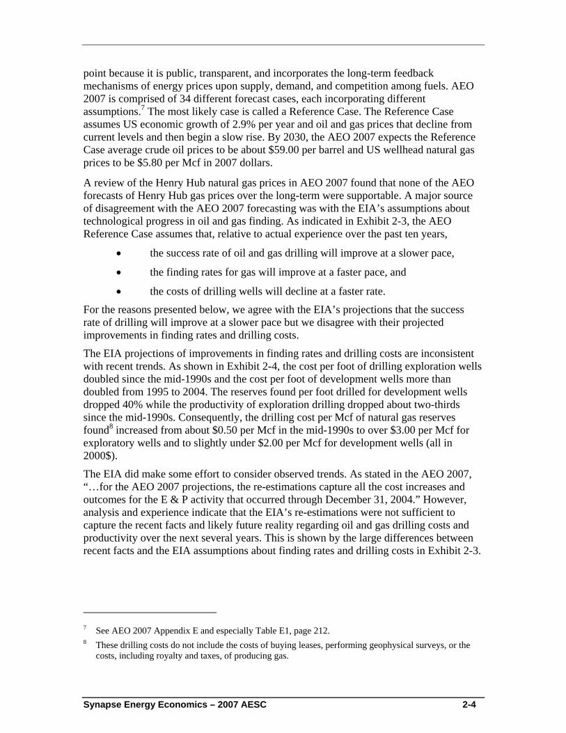
The EIA projections of improvements in finding rates and drilling costs are inconsistent with recent trends. As shown in Exhibit 2-4, the cost per foot of drilling exploration wells doubled since the mid-1990s and the cost per foot of development wells more than doubled from 1995 to 2004. The reserves found per foot drilled for development wells dropped 40% while the productivity of exploration drilling dropped about two-thirds since the mid-1990s. Consequently, the drilling cost per Mcf of natural gas reserves found8 increased from about $0.50 per Mcf in the mid-1990s to over $3.00 per Mcf for exploratory wells and to slightly under $2.00 per Mcf for development wells (all in 2000$).
The EIA did make some effort to consider observed trends. As stated in the AEO 2007, “…for the AEO 2007 projections, the re-estimations capture all the cost increases and outcomes for the E & P activity that occurred through December 31, 2004.” However, analysis and experience indicate that the EIA’s re-estimations were not sufficient to capture the recent facts and likely future reality regarding oil and gas drilling costs and productivity over the next several years. This is shown by the large differences between recent facts and the EIA assumptions about finding rates and drilling costs in Exhibit 2-3.
7 See AEO 2007 Appendix E and especially Table E1, page 212. 8 These drilling costs do not include the costs of buying leases, performing geophysical surveys, or the
costs, including royalty and taxes, of producing gas.
Synapse Energy Economics – 2007 AESC 2-5
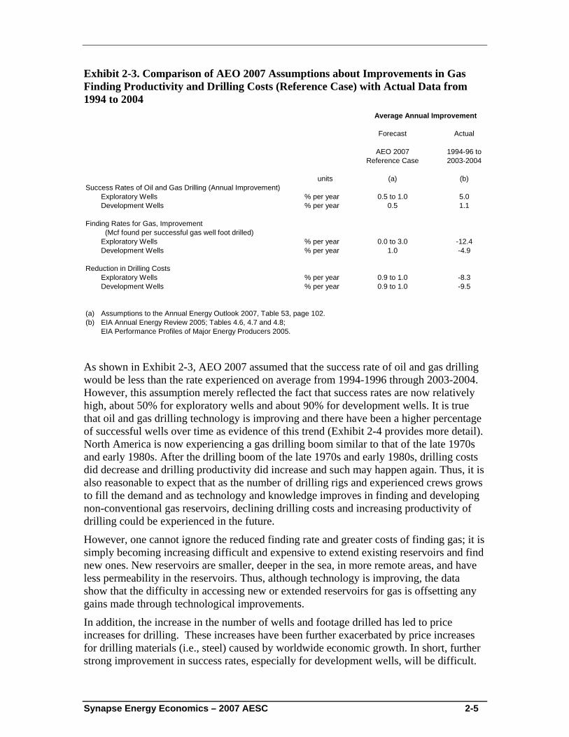
Exhibit 2-3. Comparison of AEO 2007 Assumptions about Improvements in Gas Finding Productivity and Drilling Costs (Reference Case) with Actual Data from 1994 to 2004
Forecast Actual
units (a) (b)Success Rates of Oil and Gas Drilling (Annual Improvement)
Exploratory Wells % per year 0.5 to 1.0 5.0Development Wells % per year 0.5 1.1
Finding Rates for Gas, Improvement (Mcf found per successful gas well foot drilled)Exploratory Wells % per year 0.0 to 3.0 -12.4Development Wells % per year 1.0 -4.9
Reduction in Drilling CostsExploratory Wells % per year 0.9 to 1.0 -8.3Development Wells % per year 0.9 to 1.0 -9.5
(a) Assumptions to the Annual Energy Outlook 2007, Table 53, page 102.(b) EIA Annual Energy Review 2005; Tables 4.6, 4.7 and 4.8;
EIA Performance Profiles of Major Energy Producers 2005.
1994-96 to 2003-2004
AEO 2007 Reference Case
Average Annual Improvement
As shown in Exhibit 2-3, AEO 2007 assumed that the success rate of oil and gas drilling would be less than the rate experienced on average from 1994-1996 through 2003-2004. However, this assumption merely reflected the fact that success rates are now relatively high, about 50% for exploratory wells and about 90% for development wells. It is true that oil and gas drilling technology is improving and there have been a higher percentage of successful wells over time as evidence of this trend (Exhibit 2-4 provides more detail). North America is now experiencing a gas drilling boom similar to that of the late 1970s and early 1980s. After the drilling boom of the late 1970s and early 1980s, drilling costs did decrease and drilling productivity did increase and such may happen again. Thus, it is also reasonable to expect that as the number of drilling rigs and experienced crews grows to fill the demand and as technology and knowledge improves in finding and developing non-conventional gas reservoirs, declining drilling costs and increasing productivity of drilling could be experienced in the future.
However, one cannot ignore the reduced finding rate and greater costs of finding gas; it is simply becoming increasing difficult and expensive to extend existing reservoirs and find new ones. New reservoirs are smaller, deeper in the sea, in more remote areas, and have less permeability in the reservoirs. Thus, although technology is improving, the data show that the difficulty in accessing new or extended reservoirs for gas is offsetting any gains made through technological improvements.
In addition, the increase in the number of wells and footage drilled has led to price increases for drilling. These increases have been further exacerbated by price increases for drilling materials (i.e., steel) caused by worldwide economic growth. In short, further strong improvement in success rates, especially for development wells, will be difficult.
Synapse Energy Economics – 2007 AESC 2-6
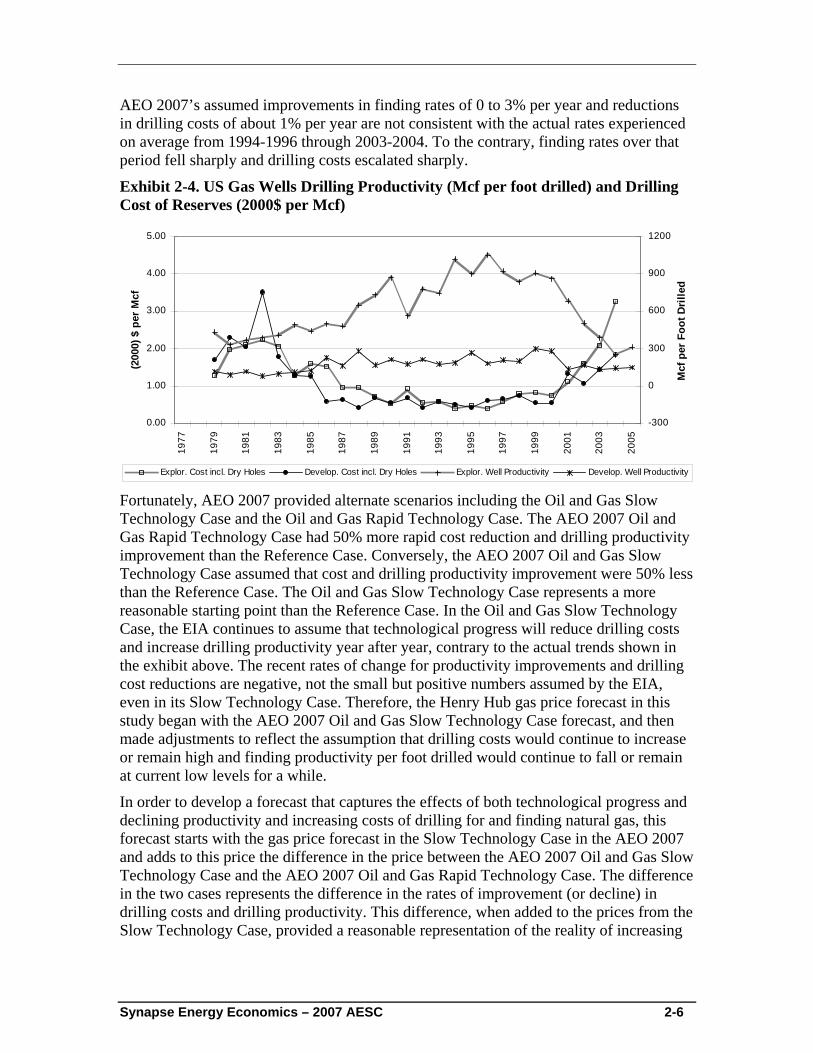
AEO 2007’s assumed improvements in finding rates of 0 to 3% per year and reductions in drilling costs of about 1% per year are not consistent with the actual rates experienced on average from 1994-1996 through 2003-2004. To the contrary, finding rates over that period fell sharply and drilling costs escalated sharply.
Exhibit 2-4. US Gas Wells Drilling Productivity (Mcf per foot drilled) and Drilling Cost of Reserves (2000$ per Mcf)
0.00
1.00
2.00
3.00
4.00
5.00
1977
1979
1981
1983
1985
1987
1989
1991
1993
1995
1997
1999
2001
2003
2005
(200
0) $
per
Mcf
-300
0
300
600
900
1200
Mcf
per
Foo
t Dril
led
Explor. Cost incl. Dry Holes Develop. Cost incl. Dry Holes Explor. Well Productivity Develop. Well Productivity Fortunately, AEO 2007 provided alternate scenarios including the Oil and Gas Slow Technology Case and the Oil and Gas Rapid Technology Case. The AEO 2007 Oil and Gas Rapid Technology Case had 50% more rapid cost reduction and drilling productivity improvement than the Reference Case. Conversely, the AEO 2007 Oil and Gas Slow Technology Case assumed that cost and drilling productivity improvement were 50% less than the Reference Case. The Oil and Gas Slow Technology Case represents a more reasonable starting point than the Reference Case. In the Oil and Gas Slow Technology Case, the EIA continues to assume that technological progress will reduce drilling costs and increase drilling productivity year after year, contrary to the actual trends shown in the exhibit above. The recent rates of change for productivity improvements and drilling cost reductions are negative, not the small but positive numbers assumed by the EIA, even in its Slow Technology Case. Therefore, the Henry Hub gas price forecast in this study began with the AEO 2007 Oil and Gas Slow Technology Case forecast, and then made adjustments to reflect the assumption that drilling costs would continue to increase or remain high and finding productivity per foot drilled would continue to fall or remain at current low levels for a while.
In order to develop a forecast that captures the effects of both technological progress and declining productivity and increasing costs of drilling for and finding natural gas, this forecast starts with the gas price forecast in the Slow Technology Case in the AEO 2007 and adds to this price the difference in the price between the AEO 2007 Oil and Gas Slow Technology Case and the AEO 2007 Oil and Gas Rapid Technology Case. The difference in the two cases represents the difference in the rates of improvement (or decline) in drilling costs and drilling productivity. This difference, when added to the prices from the Slow Technology Case, provided a reasonable representation of the reality of increasing
Synapse Energy Economics – 2007 AESC 2-7
drilling costs and declining drilling productivity in the recent past and near future. The result is representative of the Henry Hub natural gas price under “a less than Slow Technology Case.” In other words, the Henry Hub natural gas price under “a less than Slow Technology Case” will be above the Slow Technology Case forecast price by the same differential as the Henry Hub natural gas price under the “Rapid Technology Case” is below the Slow Technology Case forecast price. A forecast that provides a reasonable reflection of the likely price impacts of increasing drilling costs and declining drilling productivity was developed by adding the price differential to the Slow Technology Case forecast price.
As a check on the validity of this forecast, the forecast prices for 2007-2012 were compared to the Henry Hub futures prices from NYMEX.9 Annual averages using actual monthly NYMEX prices for January through March 2007 and NYMEX futures prices for April 2007 through December 201210 were calculated. This comparison indicated that near-term prices forecast under the methodology outlined above for 2007 through 2012 were, on average, 98% of the Henry Hub futures prices as of mid-March 200711 when expressed in 2007$. Although this is a modest discrepancy, it was determined that the optimal approach would be to use a combination of Henry Hub futures prices in the near-term (2007-2012) and projections derived from the AEO 2007 Oil and Gas Slow Technology Case described above in the long-term (2013-2022).
ii. Annual Henry Hub Natural Gas Price Forecast
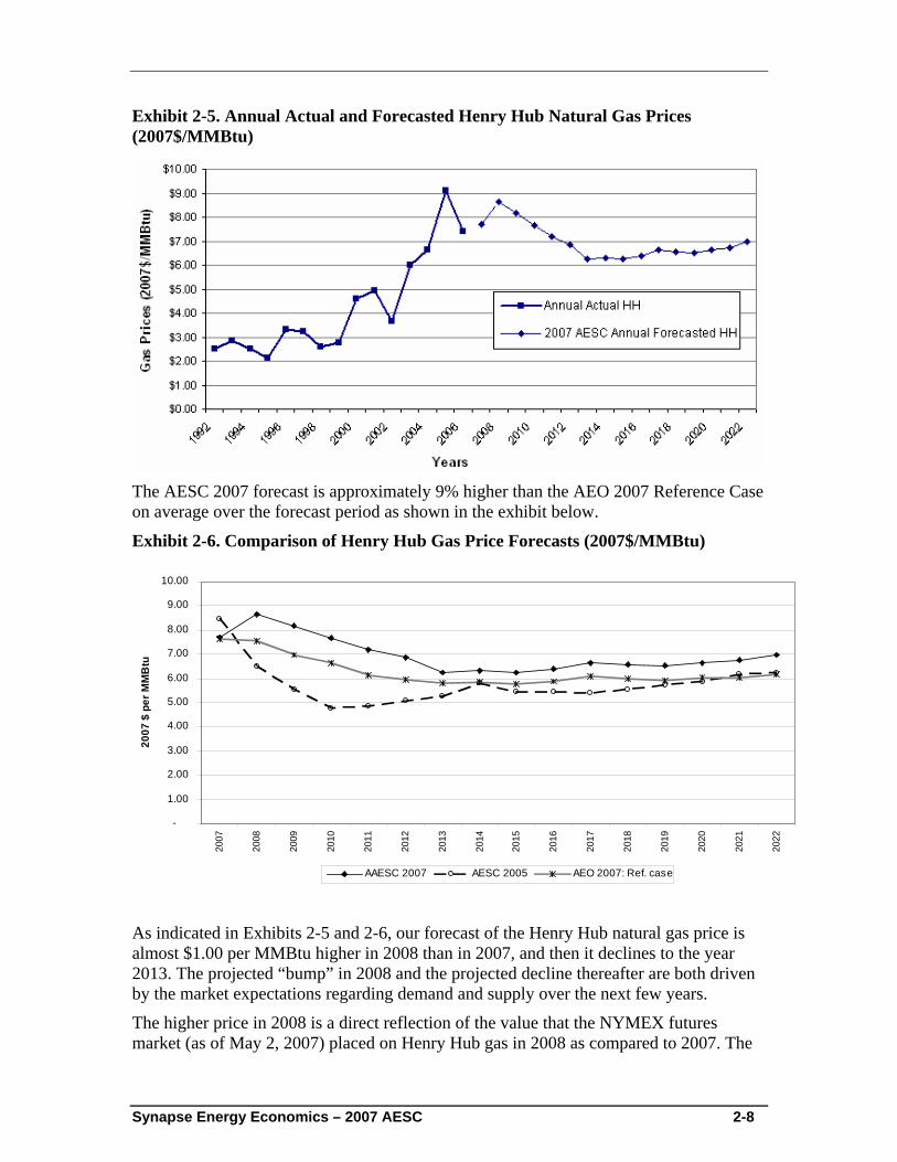
The AESC 2007 Henry Hub annual natural gas price forecast is shown in the exhibit below relative to the actual Henry Hub prices from 1992 through 2006. Actual Henry Hub prices were in the $3.00/MMBtu (2007$) range from 1992 through 1999, and have increased steadily since then. The AESC 2007 forecast projects that prices decline to the $6.00 to $7.00/MMBtu range, and then stabilize at that level through 2022.
9 The futures market represents the consensus of market participants who do have a reasonable
knowledge of near-term market and industry facts. See the paper by Adam Sieminski, “Varying Views on the Future of the Natural Gas Market: Secrets of Energy Price Forecasting,” 2007 EIA Energy Outlook, Modeling and Data Conference, Washington DC, March 28, 2007. Available at www.eia.doe.gov/oiaf/aeo/conf/index.htm.
10 As of May 2, 2007. 11 NYMEX ClearPort market prices as of May 2, 2007.
Synapse Energy Economics – 2007 AESC 2-8
Exhibit 2-5. Annual Actual and Forecasted Henry Hub Natural Gas Prices (2007$/MMBtu)
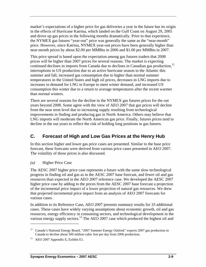
The AESC 2007 forecast is approximately 9% higher than the AEO 2007 Reference Case on average over the forecast period as shown in the exhibit below.
Exhibit 2-6. Comparison of Henry Hub Gas Price Forecasts (2007$/MMBtu)
-
1.00
2.00
3.00
4.00
5.00
6.00
7.00
8.00
9.00
10.00
2007
2008
2009
2010
2011
2012
2013
2014
2015
2016
2017
2018
2019
2020
2021
2022
2007
$ p
er M
MB
tu
AAESC 2007 AESC 2005 AEO 2007: Ref. case
As indicated in Exhibits 2-5 and 2-6, our forecast of the Henry Hub natural gas price is almost $1.00 per MMBtu higher in 2008 than in 2007, and then it declines to the year 2013. The projected “bump” in 2008 and the projected decline thereafter are both driven by the market expectations regarding demand and supply over the next few years.
The higher price in 2008 is a direct reflection of the value that the NYMEX futures market (as of May 2, 2007) placed on Henry Hub gas in 2008 as compared to 2007. The
Synapse Energy Economics – 2007 AESC 2-9
market’s expectations of a higher price for gas deliveries a year in the future has its origin in the effects of Hurricane Katrina, which landed on the Gulf Coast on August 29, 2005 and drove up gas prices in the following months dramatically. Prior to that experience, the NYMEX gas futures “year-out” price was generally the same as the “near-month” price. However, since Katrina, NYMEX year-out prices have been generally higher than near-month prices by about $2.00 per MMBtu in 2006 and $1.00 per MMBtu in 2007.
This price spread is based upon the expectation among gas futures traders that 2008 prices will be higher than 2007 prices for several reasons. The market is expecting continued declines in imports from Canada due to declines in Canadian gas production,12 interruptions in US production due to an active hurricane season in the Atlantic this summer and fall, increased gas consumption due to higher than normal summer temperatures in the United States and high oil prices, decreases in LNG imports due to increases in demand for LNG in Europe to meet winter demand, and increased US consumption this winter due to a return to average temperatures after the recent warmer than normal winters.
There are several reasons for the decline in the NYMEX gas futures prices for the out years beyond 2008. Some agree with the view of AEO 2007 that gas prices will decline from the near term level due to increasing supply resulting from technological improvements in finding and producing gas in North America. Others may believe that LNG imports will moderate the North American gas price. Finally, futures prices tend to decline in the out years to reflect the risk of holding long positions in gas futures.
C. Forecast of High and Low Gas Prices at the Henry Hub In this section higher and lower gas price cases are presented. Similar to the base price forecast, these forecasts were derived from various price cases presented in AEO 2007. The volatility of those prices is also discussed.
(a) Higher Price Case
The AESC 2007 higher price case represents a future with the same slow technological progress in finding oil and gas as in the AESC 2007 base forecast, and fewer oil and gas resources than expected in the AEO 2007 reference case. We developed the AESC 2007 higher price case by adding to the prices from the AESC 2007 base forecast a projection of the incremental price impact of a lower projection of natural gas resources. We drew that projected incremental price impact from an analysis of AEO 2007 forecasts for various cases.
In addition to its Reference Case, AEO 2007 presents summary results for 33 additional cases. These cases have widely varying assumptions about economic growth, oil and gas resources, energy efficiency in consuming sectors, and technological development in the various energy supply sectors.13 The AEO 2007 case which produced the highest oil and 12 Canada’s National Energy Board, “2007 Summer Energy Outlook” expects 2007 gas production in
Canada to decline about 500 million cubic feet per day from 2006 production. 13 AEO 2007 Appendix E, Exhibit E1.
Synapse Energy Economics – 2007 AESC 2-10
gas prices is called the “high price case”. In that case, the quantity of oil and gas resources14 in the US and worldwide are assumed to be 15 percent less than in the reference case. This assumption produces a crude oil price of $100/bbl in 2030 compared with the Reference Case price of $59/bbl in 2030 (all in 2005$).
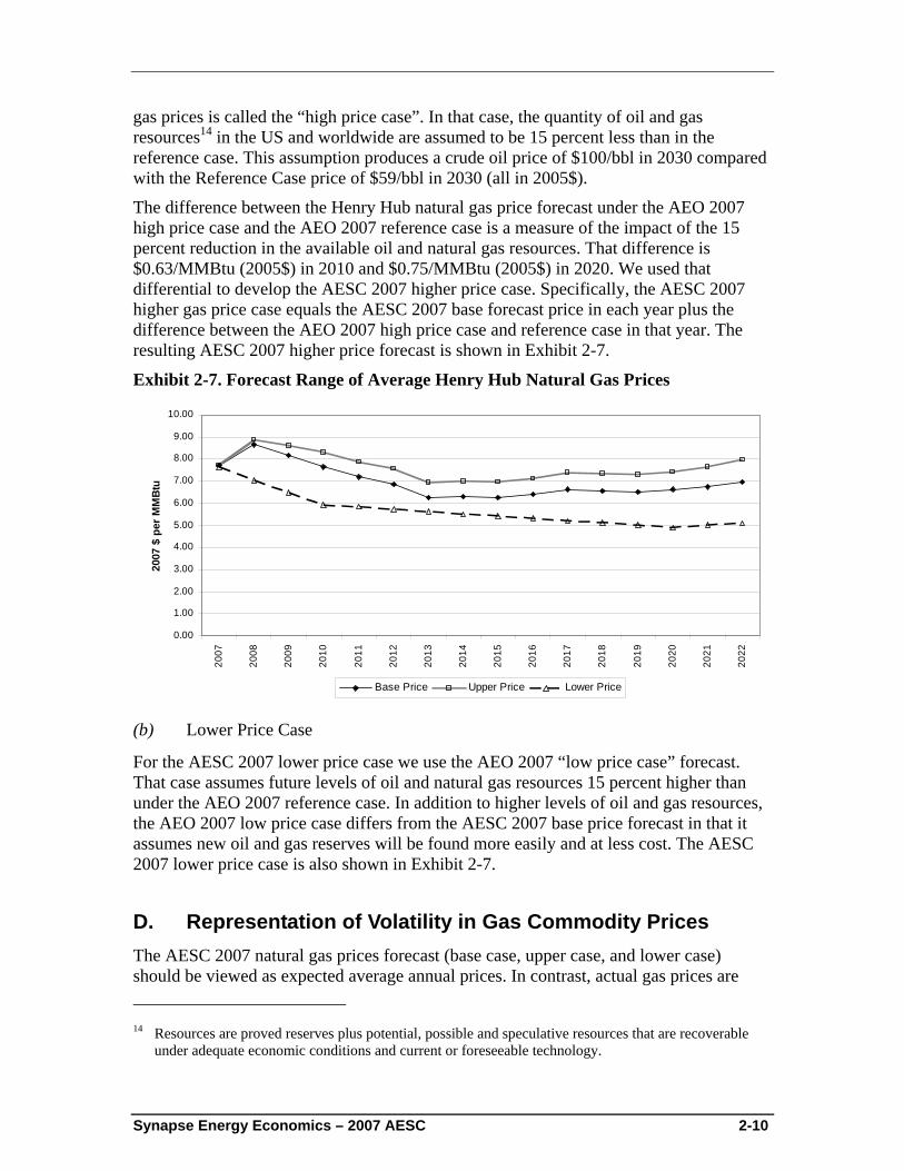
The difference between the Henry Hub natural gas price forecast under the AEO 2007 high price case and the AEO 2007 reference case is a measure of the impact of the 15 percent reduction in the available oil and natural gas resources. That difference is $0.63/MMBtu (2005$) in 2010 and $0.75/MMBtu (2005$) in 2020. We used that differential to develop the AESC 2007 higher price case. Specifically, the AESC 2007 higher gas price case equals the AESC 2007 base forecast price in each year plus the difference between the AEO 2007 high price case and reference case in that year. The resulting AESC 2007 higher price forecast is shown in Exhibit 2-7.
Exhibit 2-7. Forecast Range of Average Henry Hub Natural Gas Prices
0.00
1.00
2.00
3.00
4.00
5.00
6.00
7.00
8.00
9.00
10.00
2007
2008
2009
2010
2011
2012
2013
2014
2015
2016
2017
2018
2019
2020
2021
2022
2007
$ p
er M
MBt
u
Base Price Upper Price Lower Price
(b) Lower Price Case
For the AESC 2007 lower price case we use the AEO 2007 “low price case” forecast. That case assumes future levels of oil and natural gas resources 15 percent higher than under the AEO 2007 reference case. In addition to higher levels of oil and gas resources, the AEO 2007 low price case differs from the AESC 2007 base price forecast in that it assumes new oil and gas reserves will be found more easily and at less cost. The AESC 2007 lower price case is also shown in Exhibit 2-7.
D. Representation of Volatility in Gas Commodity Prices The AESC 2007 natural gas prices forecast (base case, upper case, and lower case) should be viewed as expected average annual prices. In contrast, actual gas prices are 14 Resources are proved reserves plus potential, possible and speculative resources that are recoverable
under adequate economic conditions and current or foreseeable technology.
Synapse Energy Economics – 2007 AESC 2-11
volatile. Thus, it is reasonable to expect actual prices to vary around these expected annual average prices. The upper and lower price cases are not intended to show the range of volatility of gas prices. Gas prices have changed by a factor of two or more during a year and they can stay above or below the “expected” price for periods longer than a year.
Pindyck argues that oil, coal, and natural gas prices tend to move toward long-run total marginal cost.15 This behavior is consistent with the forecast of an average price but with the expectation that the actual price will vary around the average price in a random manner with an annual standard deviation of 11% to 14% even while tending to move to the average. However, Pindyck suggests that the movement of oil and gas prices to a long-run marginal cost is slow and can take up to a decade.16
Thus, assuming that the AESC 2007 base price forecast is correct, one should expect that the random movements in gas prices could send the gas price above the upper gas price shown in the exhibit above for several months or in some cases for more than a year. For example, in 2015 the base price forecast is $6.25 per MMBtu (in 2007$). A 12% random increase in that year would make the price $7.00, which is slightly greater than the $6.98 in the higher price forecast. Similarly, random movements could result in actual gas prices below the forecast price. Random movements could move prices in different directions from year to year, above and below the prices forecast for those years.
Price spikes are an example of price volatility. From time to time, the daily spot or even the monthly price of natural gas spikes. In New England and in other gas consuming areas there have been daily price spikes during very cold weather. In addition, natural gas prices have increased for longer periods. The recent example of Hurricane Katrina in 2005 is illustrative. Katrina hit the Gulf Coast on August 29, 2005. One month earlier on July 29, 2005 the NYMEX gas futures contract for September 2005 delivery was priced at $7.885 per MMBtu. On December 13, 2005 the NYMEX January 2006 gas futures contract settlement price was $15.378. Six months after Katrina struck the Gulf Coast, that is, on March 1, 2006, the April 2006 gas futures contract was priced at $6.733 per MMBtu. Subsequently 2006 experienced few hurricanes and on September 27, 2006 the October 2006 gas futures contract closed at $4.210 per MMBtu. But these prices were short lived and on March 1, 2007 the April 2007 gas futures contract settled at a price of $7.288. In this example a shock that removed 5 Bcf per day of natural gas supply produced a strong increase in prices, but prices quickly reversed to more typical levels and in less than a year gas futures price fell temporarily to a level less than one-third of the December 2005 peak. Such shocks and gas price volatility should be expected in the future. Nonetheless, the AESC 2007 base gas price forecast should be viewed as an average or expected Henry Hub gas price forecast.
15 Robert S. Pindyck, “The Long-Run Evolution of Energy Prices,” The Energy Journal, Vol. 20, No. 2
pages 1-27 (1999). 16 Pindyck shows that the random variation is similar to a geometric Brownian motion with an annual
standard deviation of 11 to 14 percent for natural gas, but with a slow movement back toward a mean, which is related to the long-run total marginal cost of the resource, pages 24-25 and 6.
Synapse Energy Economics – 2007 AESC 2-12
An adjustment to the gas price forecast was not developed for price spikes for several reasons. First, there is little, if any, analytical work publicly available on this issue. Second, the prices should be used as the basis for avoided energy supply costs in evaluating the economic value of long-term investments in energy efficiency. It is not anticipated that the levelized price of gas over the long-term, e.g., 10 to 20 years, would be materially different if one estimated increases from an occasional one to three day price spike during a cold snap or even the type of several month gas price increase following Hurricane Katrina in the fall of 2005. Reasonably high gas prices are already being forecast for the future, and it is believed that investment decisions are unlikely to be affected by accounting for price spikes. Moreover, it is also possible that gas prices could fall below the levels of this forecast (a US recession could lead to a drop in natural gas prices).
E. Forecast of Price for Electric Generation in New England The forecast natural gas prices for electric generation in New England consists of three components. A forecast of the monthly prices at the Henry Hub, a forecast of the “basis” or cost differential between the Henry Hub and New England, and a forecast of the lateral commodity charge for the delivery of the gas from the pipeline pricing point to the generating unit. The derivation of this forecast is outlined below.
i. Monthly Henry Hub Natural Gas Price Forecast
The first step in producing a forecast of monthly gas prices in New England was to translate the annual Henry Hub natural gas price forecast into a monthly Henry Hub natural gas price forecast. The monthly NYMEX actual prices from January 2007 through May 2007 and the forecasted prices from June 2007 through December 2012 were used to develop ratios of the prices in each month of a year to the annual average for that year. These ratios were applied to the forecast of annual prices from 2013 through 2022 to develop forecasts of monthly prices in each of those years.
ii. Monthly New England Regional Natural Gas Price Forecast
The next step was to develop a forecast of the basis, or cost differential, between monthly spot prices at the Henry Hub and monthly spot prices in New England. Monthly spot prices in New England are reported at several points, the most representative of which are Tennessee Gas Pipeline Zone 6 (TGP Z6) and Algonquin Gas Pipeline City Gate (ALG)17
For our forecast we assumed that the future regional spot market price in each month of the study period would equal the forecast Henry Hub price each month plus the historical average basis differential. The historical average basis differential is equal to the
17 Zone 6 of the Tennessee Gas Pipeline is the section serving New England. Algonquin is a regional
pipeline serving New England.
Synapse Energy Economics – 2007 AESC 2-13
difference between actual monthly Henry Hub natural gas prices and actual monthly regional spot prices as reported at TGP Z6 and ALG respectively.
Our analyses indicate that the historical average basis differential is most accurately represented as a ratio rather than as an absolute differential. Therefore, our forecast of the regional monthly spot prices, with the exception of Vermont, was calculated by taking the average of the forecasts for prices of spot gas delivered from TGP Z6 and ALG.
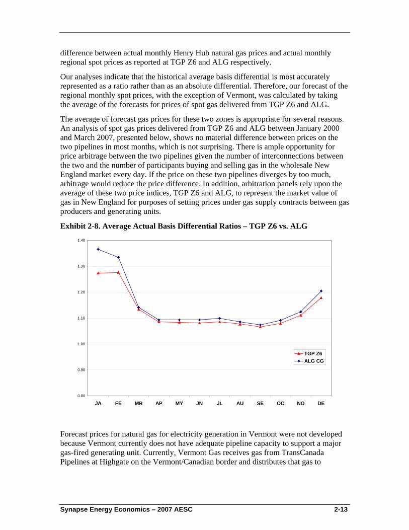
The average of forecast gas prices for these two zones is appropriate for several reasons. An analysis of spot gas prices delivered from TGP Z6 and ALG between January 2000 and March 2007, presented below, shows no material difference between prices on the two pipelines in most months, which is not surprising. There is ample opportunity for price arbitrage between the two pipelines given the number of interconnections between the two and the number of participants buying and selling gas in the wholesale New England market every day. If the price on these two pipelines diverges by too much, arbitrage would reduce the price difference. In addition, arbitration panels rely upon the average of these two price indices, TGP Z6 and ALG, to represent the market value of gas in New England for purposes of setting prices under gas supply contracts between gas producers and generating units.
Exhibit 2-8. Average Actual Basis Differential Ratios – TGP Z6 vs. ALG
0.80
0.90
1.00
1.10
1.20
1.30
1.40
JA FE MR AP MY JN JL AU SE OC NO DE
TGP Z6ALG CG
Forecast prices for natural gas for electricity generation in Vermont were not developed because Vermont currently does not have adequate pipeline capacity to support a major gas-fired generating unit. Currently, Vermont Gas receives gas from TransCanada Pipelines at Highgate on the Vermont/Canadian border and distributes that gas to
Synapse Energy Economics – 2007 AESC 2-14
customers in northern Vermont. It is not connected to the rest of the New England gas pipeline network.
In order to adjust the Henry Hub natural gas prices as accurately as possible, both actual monthly basis differentials (the absolute difference between TGP Z6 and ALG and Henry Hub prices in $/MMBtu) and monthly basis differential ratios (TGP Z6 and ALG versus Henry Hub prices) were calculated over the period January 2000 – March 2007. In the end, the basis differential ratios were utilized instead of the actual monthly basis differentials due to the fact that they were more stable over time. The average monthly basis differential ratios for TGP Z6 and ALG were applied to the monthly forecast of Henry Hub natural gas prices to develop monthly prices for TGP Z6 and TLG over the forecast period.
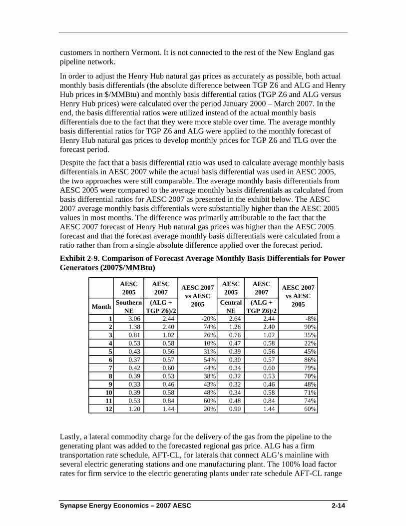
Despite the fact that a basis differential ratio was used to calculate average monthly basis differentials in AESC 2007 while the actual basis differential was used in AESC 2005, the two approaches were still comparable. The average monthly basis differentials from AESC 2005 were compared to the average monthly basis differentials as calculated from basis differential ratios for AESC 2007 as presented in the exhibit below. The AESC 2007 average monthly basis differentials were substantially higher than the AESC 2005 values in most months. The difference was primarily attributable to the fact that the AESC 2007 forecast of Henry Hub natural gas prices was higher than the AESC 2005 forecast and that the forecast average monthly basis differentials were calculated from a ratio rather than from a single absolute difference applied over the forecast period.
Exhibit 2-9. Comparison of Forecast Average Monthly Basis Differentials for Power Generators (2007$/MMBtu)
AESC 2005
AESC 2007
AESC 2005
AESC 2007
Month Southern NE
(ALG + TGP Z6)/2
Central NE
(ALG + TGP Z6)/2
1 3.06 2.44 -20% 2.64 2.44 -8%2 1.38 2.40 74% 1.26 2.40 90%3 0.81 1.02 26% 0.76 1.02 35%4 0.53 0.58 10% 0.47 0.58 22%5 0.43 0.56 31% 0.39 0.56 45%6 0.37 0.57 54% 0.30 0.57 86%7 0.42 0.60 44% 0.34 0.60 79%8 0.39 0.53 38% 0.32 0.53 70%9 0.33 0.46 43% 0.32 0.46 48%
10 0.39 0.58 48% 0.34 0.58 71%11 0.53 0.84 60% 0.48 0.84 74%12 1.20 1.44 20% 0.90 1.44 60%
AESC 2007 vs AESC
2005
AESC 2007 vs AESC
2005
Lastly, a lateral commodity charge for the delivery of the gas from the pipeline to the generating plant was added to the forecasted regional gas price. ALG has a firm transportation rate schedule, AFT-CL, for laterals that connect ALG’s mainline with several electric generating stations and one manufacturing plant. The 100% load factor rates for firm service to the electric generating plants under rate schedule AFT-CL range
Synapse Energy Economics – 2007 AESC 2-15
in price from $0.0229 to $0.1093 per MMBtu.18 Considering that the deliveries are likely to be at less than 100 percent load factor, the $0.07 per MMBtu lateral charge used in AESC 2005 was reasonable and was adopted in AESC 2007.
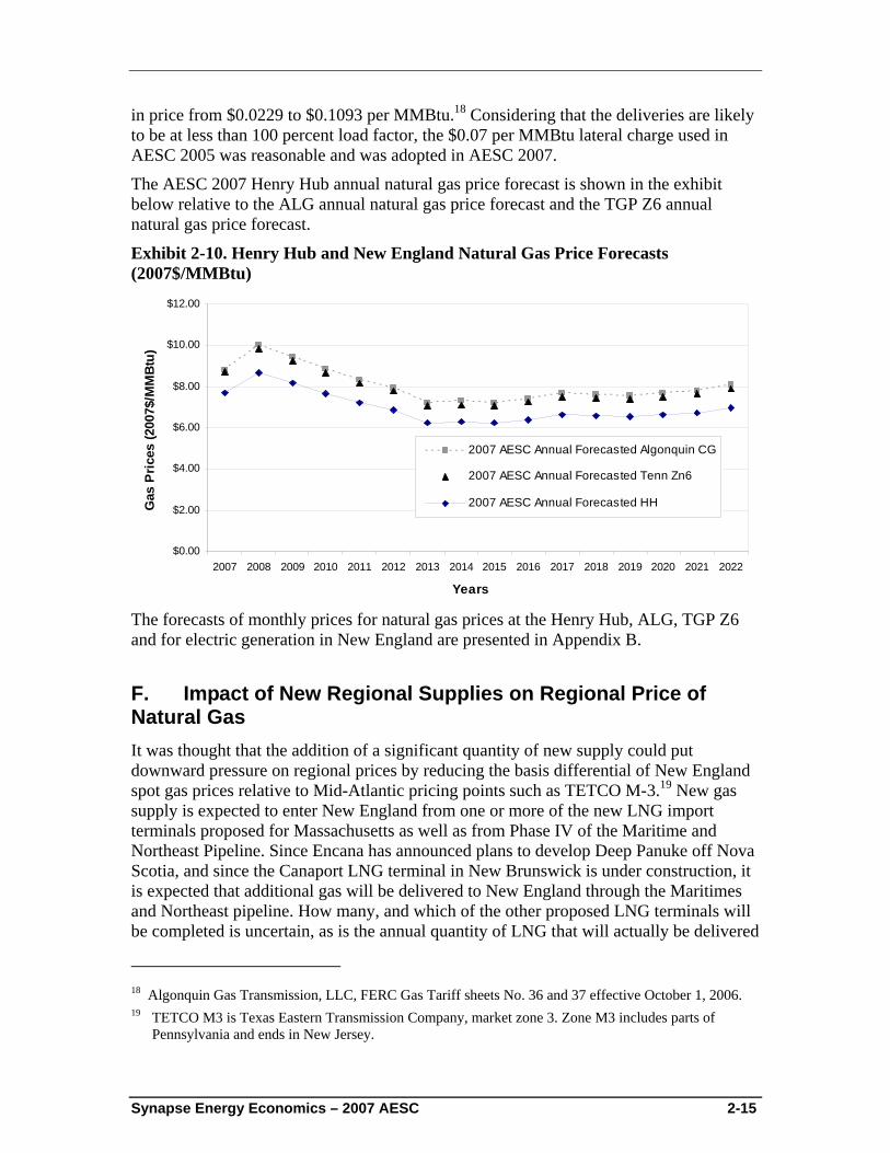
The AESC 2007 Henry Hub annual natural gas price forecast is shown in the exhibit below relative to the ALG annual natural gas price forecast and the TGP Z6 annual natural gas price forecast.
Exhibit 2-10. Henry Hub and New England Natural Gas Price Forecasts (2007$/MMBtu)
$0.00
$2.00
$4.00
$6.00
$8.00
$10.00
$12.00
2007 2008 2009 2010 2011 2012 2013 2014 2015 2016 2017 2018 2019 2020 2021 2022
Years
Gas
Pric
es (2
007$
/MM
Btu
)
2007 AESC Annual Forecasted Algonquin CG
2007 AESC Annual Forecasted Tenn Zn6
2007 AESC Annual Forecasted HH
The forecasts of monthly prices for natural gas prices at the Henry Hub, ALG, TGP Z6 and for electric generation in New England are presented in Appendix B.
F. Impact of New Regional Supplies on Regional Price of Natural Gas It was thought that the addition of a significant quantity of new supply could put downward pressure on regional prices by reducing the basis differential of New England spot gas prices relative to Mid-Atlantic pricing points such as TETCO M-3.19 New gas supply is expected to enter New England from one or more of the new LNG import terminals proposed for Massachusetts as well as from Phase IV of the Maritime and Northeast Pipeline. Since Encana has announced plans to develop Deep Panuke off Nova Scotia, and since the Canaport LNG terminal in New Brunswick is under construction, it is expected that additional gas will be delivered to New England through the Maritimes and Northeast pipeline. How many, and which of the other proposed LNG terminals will be completed is uncertain, as is the annual quantity of LNG that will actually be delivered
18 Algonquin Gas Transmission, LLC, FERC Gas Tariff sheets No. 36 and 37 effective October 1, 2006. 19 TETCO M3 is Texas Eastern Transmission Company, market zone 3. Zone M3 includes parts of
Pennsylvania and ends in New Jersey.
Synapse Energy Economics – 2007 AESC 2-16
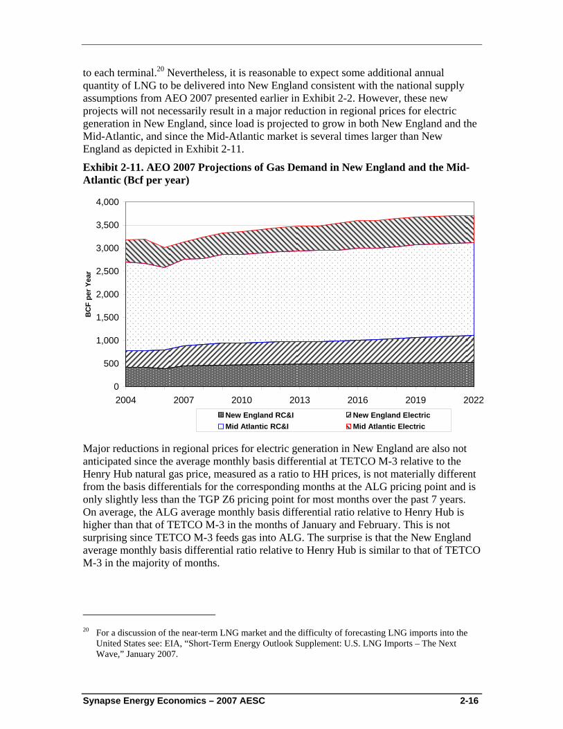
to each terminal.20 Nevertheless, it is reasonable to expect some additional annual quantity of LNG to be delivered into New England consistent with the national supply assumptions from AEO 2007 presented earlier in Exhibit 2-2. However, these new projects will not necessarily result in a major reduction in regional prices for electric generation in New England, since load is projected to grow in both New England and the Mid-Atlantic, and since the Mid-Atlantic market is several times larger than New England as depicted in Exhibit 2-11.
Exhibit 2-11. AEO 2007 Projections of Gas Demand in New England and the Mid-Atlantic (Bcf per year)
0
500
1,000
1,500
2,000
2,500
3,000
3,500
4,000
2004 2007 2010 2013 2016 2019 2022
BC
F pe
r Yea
r
New England RC&I New England ElectricMid Atlantic RC&I Mid Atlantic Electric
Major reductions in regional prices for electric generation in New England are also not anticipated since the average monthly basis differential at TETCO M-3 relative to the Henry Hub natural gas price, measured as a ratio to HH prices, is not materially different from the basis differentials for the corresponding months at the ALG pricing point and is only slightly less than the TGP Z6 pricing point for most months over the past 7 years. On average, the ALG average monthly basis differential ratio relative to Henry Hub is higher than that of TETCO M-3 in the months of January and February. This is not surprising since TETCO M-3 feeds gas into ALG. The surprise is that the New England average monthly basis differential ratio relative to Henry Hub is similar to that of TETCO M-3 in the majority of months.
20 For a discussion of the near-term LNG market and the difficulty of forecasting LNG imports into the
United States see: EIA, “Short-Term Energy Outlook Supplement: U.S. LNG Imports – The Next Wave,” January 2007.
Synapse Energy Economics – 2007 AESC 2-17
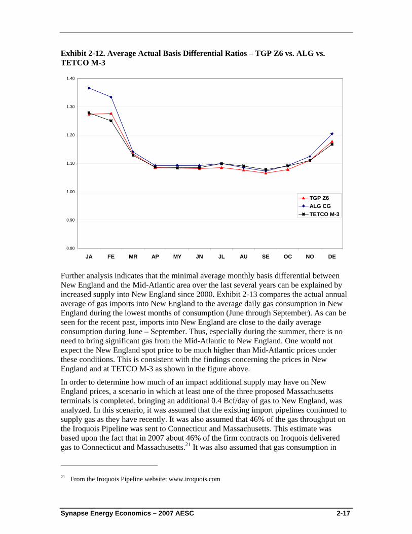
Exhibit 2-12. Average Actual Basis Differential Ratios – TGP Z6 vs. ALG vs. TETCO M-3
0.80
0.90
1.00
1.10
1.20
1.30
1.40
JA FE MR AP MY JN JL AU SE OC NO DE
TGP Z6ALG CGTETCO M-3
Further analysis indicates that the minimal average monthly basis differential between New England and the Mid-Atlantic area over the last several years can be explained by increased supply into New England since 2000. Exhibit 2-13 compares the actual annual average of gas imports into New England to the average daily gas consumption in New England during the lowest months of consumption (June through September). As can be seen for the recent past, imports into New England are close to the daily average consumption during June – September. Thus, especially during the summer, there is no need to bring significant gas from the Mid-Atlantic to New England. One would not expect the New England spot price to be much higher than Mid-Atlantic prices under these conditions. This is consistent with the findings concerning the prices in New England and at TETCO M-3 as shown in the figure above.
In order to determine how much of an impact additional supply may have on New England prices, a scenario in which at least one of the three proposed Massachusetts terminals is completed, bringing an additional 0.4 Bcf/day of gas to New England, was analyzed. In this scenario, it was assumed that the existing import pipelines continued to supply gas as they have recently. It was also assumed that 46% of the gas throughput on the Iroquois Pipeline was sent to Connecticut and Massachusetts. This estimate was based upon the fact that in 2007 about 46% of the firm contracts on Iroquois delivered gas to Connecticut and Massachusetts.21 It was also assumed that gas consumption in
21 From the Iroquois Pipeline website: www.iroquois.com
Synapse Energy Economics – 2007 AESC 2-18
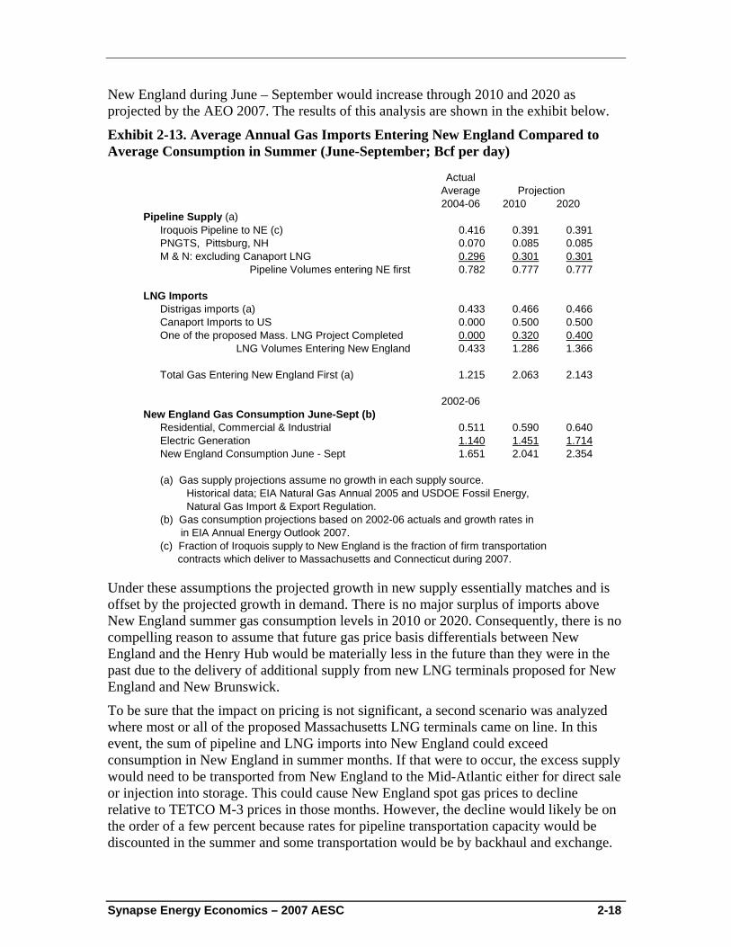
New England during June – September would increase through 2010 and 2020 as projected by the AEO 2007. The results of this analysis are shown in the exhibit below.
Exhibit 2-13. Average Annual Gas Imports Entering New England Compared to Average Consumption in Summer (June-September; Bcf per day)
ActualAverage2004-06 2010 2020
Pipeline Supply (a)Iroquois Pipeline to NE (c) 0.416 0.391 0.391PNGTS, Pittsburg, NH 0.070 0.085 0.085M & N: excluding Canaport LNG 0.296 0.301 0.301
Pipeline Volumes entering NE first 0.782 0.777 0.777
LNG ImportsDistrigas imports (a) 0.433 0.466 0.466Canaport Imports to US 0.000 0.500 0.500One of the proposed Mass. LNG Project Completed 0.000 0.320 0.400
LNG Volumes Entering New England 0.433 1.286 1.366
Total Gas Entering New England First (a) 1.215 2.063 2.143
2002-06New England Gas Consumption June-Sept (b)
Residential, Commercial & Industrial 0.511 0.590 0.640Electric Generation 1.140 1.451 1.714New England Consumption June - Sept 1.651 2.041 2.354
(a) Gas supply projections assume no growth in each supply source. Historical data; EIA Natural Gas Annual 2005 and USDOE Fossil Energy, Natural Gas Import & Export Regulation.(b) Gas consumption projections based on 2002-06 actuals and growth rates in in EIA Annual Energy Outlook 2007.(c) Fraction of Iroquois supply to New England is the fraction of firm transportation contracts which deliver to Massachusetts and Connecticut during 2007.
Projection
Under these assumptions the projected growth in new supply essentially matches and is offset by the projected growth in demand. There is no major surplus of imports above New England summer gas consumption levels in 2010 or 2020. Consequently, there is no compelling reason to assume that future gas price basis differentials between New England and the Henry Hub would be materially less in the future than they were in the past due to the delivery of additional supply from new LNG terminals proposed for New England and New Brunswick.
To be sure that the impact on pricing is not significant, a second scenario was analyzed where most or all of the proposed Massachusetts LNG terminals came on line. In this event, the sum of pipeline and LNG imports into New England could exceed consumption in New England in summer months. If that were to occur, the excess supply would need to be transported from New England to the Mid-Atlantic either for direct sale or injection into storage. This could cause New England spot gas prices to decline relative to TETCO M-3 prices in those months. However, the decline would likely be on the order of a few percent because rates for pipeline transportation capacity would be discounted in the summer and some transportation would be by backhaul and exchange.
Synapse Energy Economics – 2007 AESC 2-19
Alternatively, the LNG suppliers might choose not to deliver supplies in excess of New England demand at a price less than TETCO M-3, and instead sell some of that supply in markets with higher prices such as Europe.
G. Forecast of Price for Retail Sectors
i. Cost to Supply Natural Gas to LDCs
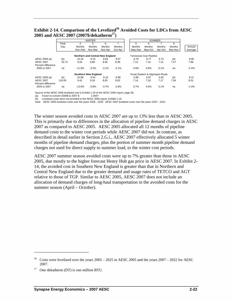
New England LDCs use three basic supply resources to meet the sendout requirements of their customers. These resources are (1) gas delivered directly from producing areas via long-haul pipelines, (2) gas withdrawn from underground storage facilities (most of which are located in Pennsylvania) and delivered by pipeline, and (3) gas stored as liquefied natural gas and/or propane in tanks located in the LDC service territories throughout New England.
The cost of gas delivered to an LDC using pipeline transportation and storage facilities consists of four basic components:
• the cost of the gas commodity, which in this study is the forecast price at the Henry Hub in Louisiana;
• the fixed demand cost of holding pipeline transportation capacity and of storage and withdrawal capacity;
• the usage (volumetric) charges for transporting gas on a pipeline and for storage injections and withdrawals; and
• the fraction (percentage) of volumes of gas received by a pipeline or storage facility that is retained by the facility for compressor fuel and losses. This fuel and loss retention increases the cost of gas above the Henry Hub price because more volumes of gas must be purchased at the Henry Hub than is delivered to the LDC. In the analysis that follows, the fuel and loss retention is represented as the ratio of the volumes of gas purchased at the Henry Hub to the volumes of gas delivered to the LDC.
The LDCs generally own the LNG and/or propane tanks and accompanying liquefaction and vaporization facilities. Since the bulk of the New England peak gas supply comes from LNG facilities, AESC 2007 focuses on them although in certain circumstances propane is the dominant peak gas source. The LDC pays for the construction, financing, operation and maintenance of the LNG facility as well as the cost of the gas that is loaded into the tank as LNG.
Because of the significantly increased level of winter season requirements and the variation in winter day requirements according to temperature, LDCs develop a portfolio among the three gas supply resources in order to optimize reliability and cost. Generally, long-haul pipeline transportation is used to meet customer gas requirements each month of the year and to refill underground storage and sometimes LNG tanks during the summer months. Much of the increased winter (November - March) gas demand from customers is met by transporting gas from the underground storage facilities, often
Synapse Energy Economics – 2007 AESC 2-20
located in Pennsylvania, to the LDC in New England.22 LNG and propane facilities meet daily peaking and seasonal requirements during the heaviest demand period, December through February.
Of those three resources, only long-haul pipeline transportation capacity is used in multiple applications, i.e., to provide direct supply in winter, to refill underground storage in summer, and to provide direct supply in summer. As a result, in order to determine the avoided cost of reductions in loads in various winter and summer periods, we had to begin by determining how to allocate the demand charges that LDCs incur for that capacity among those multiple applications. Our analysis of the average use of long-haul capacity by LDCs, presented in detail below, indicates that in winter months all of this capacity is used to provide direct supply while in summer months approximately 80% of this capacity is used to provide direct supply and to refill storage. Based upon that analysis, our projections of avoided costs are based upon the following allocations of the demand charges of long-haul pipelines:
• demand charges incurred in winter months are included in the avoided costs of winter months;
• twenty percent of demand charges incurred in summer months are included in the avoided costs of winter months, corresponding to the approximately 20% of physical capacity not being used in the summer either to refill storage or provide direct supply;
• demand charges associated with the quantity of long-haul capacity used to refill underground storage in summer are included in the avoided costs of gas stored underground. (The cost of that stored gas is ultimately included in the avoided costs of winter months);
• demand charges associated with the quantity of long-haul capacity used to provide direct supply in summer are not included in the avoided costs of summer months because our analysis indicates that demand charges for this capacity cannot be avoided.
ii. Sector-Specific Avoided Natural Gas Price Forecast
This section discusses forecasts of the avoided costs of natural gas saved by energy efficiency programs for the period 2007 through 2022 for both (1) gas delivered to New England local distribution companies (LDCs) and (2) the avoided cost of gas at the retail level delivered to end-users of gas. The avoided costs are calculated as a weighted average cost of the marginal natural gas supply sources during specified seasonal and peak-day costing periods.
The avoided cost of gas to an LDC is the cost of the marginal source of supply for the relevant cost period. For this analysis, the long-run avoided cost was estimated because efficiency improvement is a long-term effect that can allow an LDC to avoid both the
22 LDCs acquire pipeline and storage services through a portfolio of contracts whose terms and conditions
are regulated by the Federal Energy Regulatory Commission (FERC).
Synapse Energy Economics – 2007 AESC 2-21
short-run variable costs and also some, but not all, of the long-term fixed costs of gas supply sources. The marginal cost (avoided cost) was computed for each month and for the peak day. The avoided cost is the cost of delivering one dekatherm of gas to the LDC via the three resources in each month. For each of the winter months, November through March, when gas is supplied by the three resources, the marginal cost is the weighted average of the costs for each supply source depending upon the fraction of total volumes of sendout provided by each source. By computing the weighted average, the approach taken in AESC 2005 was mirrored by assuming that the LDCs have optimized the mix of supply sources and thus both fixed and variable costs are avoided in the mix of all three of the supply sources for a long-term efficiency improvement.23
In this forecast, the approach of AESC 2005 was applied in some areas, but not in others. For example, a different approach was taken when computing the avoided cost of each cost period. AESC 2007 estimates the avoided cost for each month and averages the monthly avoided costs.
Similar to AESC 2005, it was assumed that the marginal source of gas to New England LDCs from the Henry Hub is transportation and storage on either of the Tennessee Gas Pipeline (TGP), for LDCs in Northern and Central New England, or the route of Texas Eastern Transmission (TETCO) and Algonquin Gas Transmission (AGT), for LDCs in Southern New England.24 While proposed LNG receiving and re-gasification terminals in New England and New Brunswick will likely be new gas suppliers to New England, it is not likely that they will establish the avoided cost of gas supply to New England. Rather, the price of gas from these new terminals will be set by the price of gas in New England supplied by TGP and TETCO-ALG.25
23 In a short-run marginal cost analysis only variable costs can be adjusted and thus the avoided cost is
determined by the one supply source which has the highest variable cost. 24 Northern and Central New England is Massachusetts, New Hampshire and Maine; Southern New
England is Connecticut and Rhode Island. 25 Unlike in the past, the Federal Energy Regulatory Commission has decided that LNG terminals will not
need to offer open access services and will be able to sell LNG at market prices. In a similar fashion the Maritimes & Northeast pipeline expansion is contracted by Repsol YPF, which is the provider of the LNG to the Canaport LNG terminal in New Brunswick. Thus this LNG will also be sold at market prices in New England.
Synapse Energy Economics – 2007 AESC 2-22
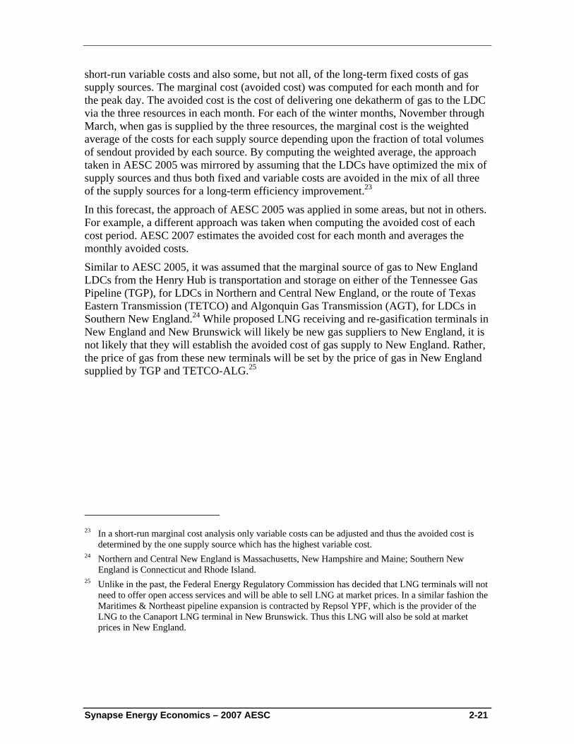
Exhibit 2-14. Comparison of the Levelized26 Avoided Costs for LDCs from AESC 2005 and AESC 2007 (2007$/dekatherm27)
Peak 3 5 6 7 5 6 7 9Day Months Months Months Months Months Months Months Months Annual
Dec-Feb Nov-Mar Nov-Apr Oct-Apr May-Sep May-Oct Apr-Oct Mar-Nov Average
Northern and Central New England Tennessee Gas PipelineAESC 2005 (a) (b) 10.26 9.15 8.84 8.57 6.79 6.77 6.74 (b) 8.06AESC 2007 92.72 9.04 8.86 8.56 8.39 7.12 7.16 7.15 7.47 7.86Percent difference 2005 to 2007 na -11.9% -3.2% -3.1% -2.1% 4.9% 5.8% 6.1% na -2.4%
Southern New England Texas Eastern & Algonquin RouteAESC 2005 (a) (b) 10.88 9.55 9.18 8.88 6.89 6.87 6.82 (b) 8.12AESC 2007 110.05 9.41 9.18 8.83 8.63 7.14 7.18 7.17 7.54 8.01Percent difference 2005 to 2007 na -13.6% -3.8% -3.7% -2.8% 3.7% 4.6% 5.1% na -1.4%
Source of the AESC 2005 levelized cost is Exhibit 1-19 of the AESC 2005 report, page 38.(a) Factor to convert 2005$ to 2007 $ 1.0547(b) Levelized costs were not provided in the AESC 2005 report, Exhibit 1-19.Note: AESC 2005 levelized costs over the years 2005 - 2025. AESC 2007 levelized costs over the years 2007 - 2022.
WINTER SUMMER
The winter season avoided costs in AESC 2007 are up to 13% less than in AESC 2005. This is primarily due to differences in the allocation of pipeline demand charges in AESC 2007 as compared to AESC 2005. AESC 2005 allocated all 12 months of pipeline demand costs to the winter cost periods while AESC 2007 did not. In contrast, as described in detail earlier in Section 2.G.i., AESC 2007 effectively allocated 5 winter months of pipeline demand charges, plus the portion of summer month pipeline demand charges not used for direct supply to summer load, to the winter cost periods.
AESC 2007 summer season avoided costs were up to 7% greater than those in AESC 2005, due mostly to the higher forecast Henry Hub gas price in AESC 2007. In Exhibit 2-14, the avoided cost in Southern New England is greater than that in Northern and Central New England due to the greater demand and usage rates of TETCO and AGT relative to those of TGP. Similar to AESC 2005, AESC 2007 does not include an allocation of demand charges of long-haul transportation in the avoided costs for the summer season (April – October).
26 Costs were levelized over the years 2005 – 2025 in AESC 2005 and the years 2007 – 2022 for AESC
2007. 27 One dekatherm (DT) is one million BTU.
Synapse Energy Economics – 2007 AESC 2-23
(a) Representative New England Local Distribution Company
For this avoided cost analysis a representative New England LDC was used to determine the fraction of customer requirements met from each resource each month and the fraction of storage refill in each of the summer months, April through October. The characteristics of a representative New England LDC are shown in the exhibit below.
Exhibit 2-15. Representative New England Local Gas Distribution Company Monthly Characteristics of Send-Out by Source, Peak Month, and Storage Injection
JUL AUG SEP OCT NOV DEC JAN FEB MAR APR MAY JUNFractions of LDC Send-out by Source Each Month
Pipeline Deliveries, Long-haul 1.00 1.00 1.00 1.00 0.86 0.64 0.50 0.52 0.68 1.00 1.00 1.00Underground Storage 0.00 0.00 0.00 0.00 0.11 0.33 0.40 0.39 0.30 0.00 0.00 0.00LNG and Propane Peaking Supply 0.00 0.00 0.00 0.00 0.03 0.03 0.10 0.09 0.02 0.00 0.00 0.00
Total 1.00 1.00 1.00 1.00 1.00 1.00 1.00 1.00 1.00 1.00 1.00 1.00
Fraction of Annual Sendout each Month 0.032 0.034 0.036 0.062 0.096 0.143 0.174 0.151 0.114 0.077 0.046 0.035
Monthly Sendout as a Fraction of Peak Month 0.184 0.195 0.207 0.356 0.552 0.822 1.000 0.868 0.655 0.443 0.264 0.201
Fraction of Underground Storage Injection by Month 0.170 0.170 0.140 0.100 0.000 0.000 0.000 0.000 0.000 0.080 0.170 0.170
Sources:(a) Cost of Gas Adjustment filings at Department of Public Utilities for Yankee Gas Systems, Connecticut Natural Gas Company, Bay State Gas Co., NSTAR and KeySpan Energy.
Synapse Energy Economics – 2007 AESC 2-24
The fractions portraying the representative New England LDC were essentially an average of the data in Cost of Gas Adjustment filings for Yankee Gas Services Company, Connecticut Natural Gas Corporation, Bay State Gas Company, NSTAR Gas Company and Keyspan Energy Delivery in New England.
(b) Avoided Cost of Gas from Each of the Three Sources
As described above, the avoided cost (marginal cost) consisted of the commodity cost of gas, the demand charges of pipeline transportation and storage, the volumetric cash costs of pipeline transportation and storage, and the fuel and loss retention for the various parts of bringing gas to an LDC.
(c) Commodity Cost Inputs
For this avoided cost analysis it was assumed that the marginal cost of the gas commodity was the monthly price of gas at the Henry Hub.
(d) Pipeline Rates
As described above, it was assumed that the marginal source of gas to New England LDCs is transportation and storage on either of TGP or the route of TETCO and AGT. The cost for transportation and underground storage is set by the rates charged by these pipelines and their fuel and loss retention percentages, which are shown in the exhibit below. It was assumed that these rates and retention percentages would persist for the forecast period, 2007 – 2022. This was the same assumption as in AESC 2005.
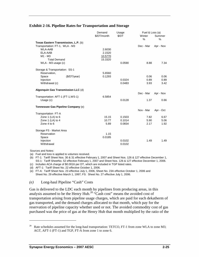
Synapse Energy Economics – 2007 AESC 2-25
Exhibit 2-16. Pipeline Rates for Transportation and Storage
Demand Usage$/DT/month $/DT Winter Summer
% %Texas Eastern Transmission, L.P. (b)Transportation: FT-1, WLA - M3 Dec - Mar Apr - Nov
WLA-AAB 2.6030ELA-AAB 2.1520M1 - M3 10.5770
Total Demand 15.3320WLA - M3 usage (c) 0.0590 8.88 7.34
Storage & Transportation: SS-1Reservation, 5.6560Space ($/DT/year) 0.1293 0.06 0.06Injection 0.0324 0.89 0.89Withdrawal (c) 0.0483 3.93 3.42
Algonquin Gas Transmission LLC (d)Dec - Mar Apr - Nov
Transportation: AFT-1 (FT-1,WS-1) 6.5854Usage (c) 0.0128 1.37 0.66
Tennessee Gas Pipeline Company (e)Nov - Mar Apr - Oct
Transportation FT-AZone 1 (LA) to 6 15.15 0.1503 7.82 6.67Zone 1 (LA) to 4 10.77 0.1014 5.90 5.06Zone 4 to 6 5.89 0.0834 2.17 1.92
Storage FS - Market AreaReservation 1.15Space 0.0185Injection 0.0102 1.49 1.49Withdrawal 0.0102
Sources and Notes:(a) Fuel and loss is applied to volumes received.(b) FT-1: Tariff Sheet Nos. 30 & 31 effective February 1, 2007 and Sheet Nos. 126 & 127 effective December 1, SS-1: Tariff SheetNo. 52 effective February 1, 2007 and Sheet Nos. 126 & 127 effective December 1, 2006.(c) Includes ACA charge of $0.0016 per DT, which are included in TGP listed rates.(d) AFT-1: Tariff Sheet No. 22 effective October 1, 2006.(e) FT-A: Tariff Sheet Nos. 23 effective July 1, 2006, Sheet No. 23A effective October 1, 2006 and
Sheet No. 29 effective March 1, 1997; FS: Sheet No. 27 effective July 1, 2006.
Fuel & Loss (a)
(e) Long-haul Pipeline “Cash” Costs
Gas is delivered to the LDC each month by pipelines from producing areas, in this analysis assumed to be the Henry Hub.28 “Cash cost” means the avoided cost of transportation arising from pipeline usage charges, which are paid for each dekatherm of gas transported, and the demand charges allocated to that month, which pay for the reservation of pipeline capacity whether used or not. The avoided commodity cost of gas purchased was the price of gas at the Henry Hub that month multiplied by the ratio of the
28 Rate schedules assumed for the long-haul transportation: TETCO, FT-1 from zone WLA to zone M3;
AGT, AFT-1 (FT-1) and TGP, FT-A from zone 1 to zone 6.
Synapse Energy Economics – 2007 AESC 2-26
Henry Hub volume purchased to one dekatherm of gas delivered to the LDC. Because of the retention of gas for fuel and loss in both transportation and storage, more than one dekatherm of gas must be purchased at the Henry Hub in order to deliver one dekatherm to the LDC.
This ratio of gas volumes purchased at the Henry Hub to one dekatherm of gas delivered to the LDC was established by the fuel and loss retention percentages of the various pipeline transportation and storage services used between the Henry Hub and the LDC. For example, assume that the gas is transported by two pipelines: A and B from the Henry Hub to the LDC. The fuel and loss percentage is 6% for A (Fa) and 4 percent for pipeline B (Fb). The fuel and loss amount taken by the pipeline is based on the volumes received by the pipeline (R) while the demand and usage charges are based on the volume of gas delivered by the pipeline (D). In order to compute the ratio of gas received to that delivered the following equations were used:
(1) D = R – FR
(2) D = R(1-F)
(3) R/D = 1/(1-F)
For pipeline A; Ra/Da = 1/(1-.06) = 1.0638; or Ra = 1.0638 Da
For pipeline B; Rb/Db = 1/(1-.04) = 1.0417; or Rb = 1.0417 Db
Since Db is the amount delivered to the LDC, Ra/Db or the ratio of the amount to be purchased in the field to the amount delivered to the LDC is what needs to be computed.
Since: Rb = Da
Ra = 1.0638 Da = (1.0638)Rb = (1.0638)(1.0417)Db
Thus: Ra/Db = (1.0638)(1.0417) = 1.1082
Or: 1.1082 DT of natural gas must be purchased for each DT delivered.
The exhibit shows the avoided costs by gas source and pipeline route.
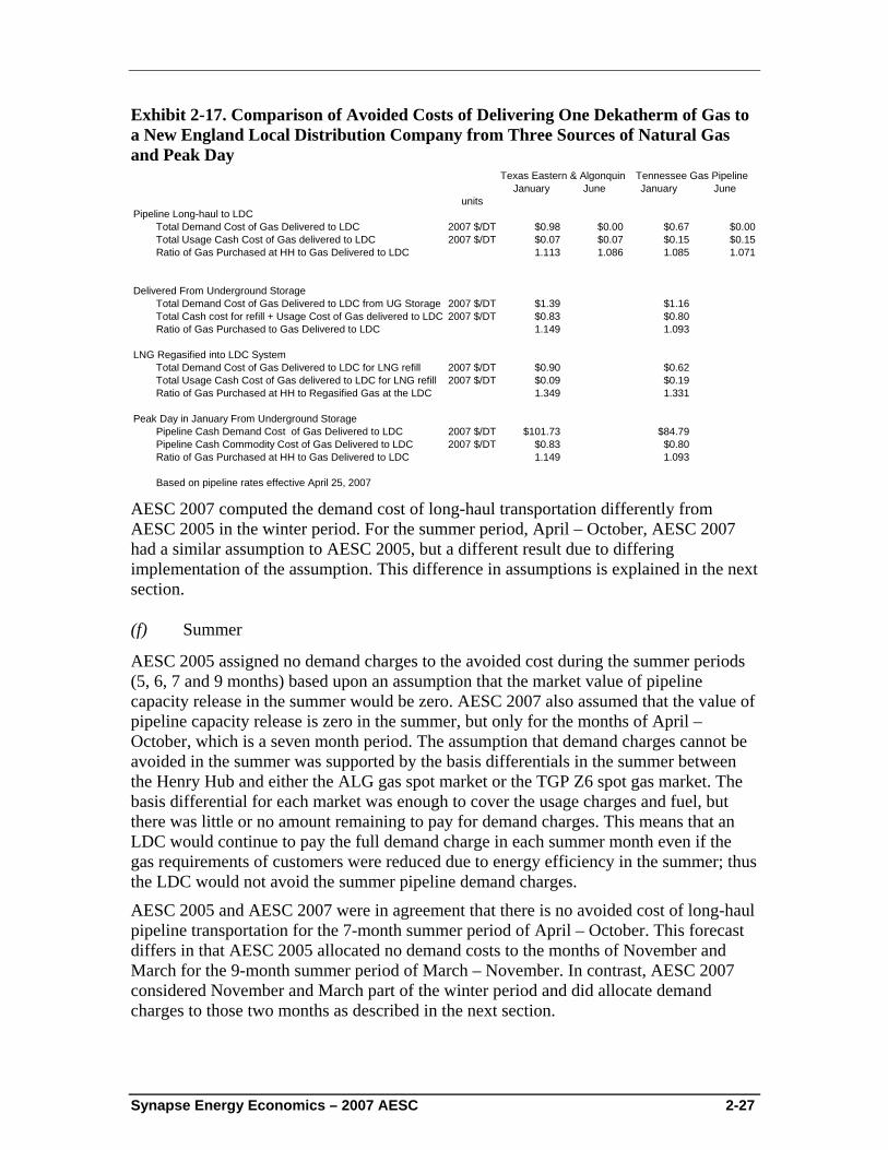
Synapse Energy Economics – 2007 AESC 2-27
Exhibit 2-17. Comparison of Avoided Costs of Delivering One Dekatherm of Gas to a New England Local Distribution Company from Three Sources of Natural Gas and Peak Day
January June January Juneunits
Pipeline Long-haul to LDCTotal Demand Cost of Gas Delivered to LDC 2007 $/DT $0.98 $0.00 $0.67 $0.00Total Usage Cash Cost of Gas delivered to LDC 2007 $/DT $0.07 $0.07 $0.15 $0.15Ratio of Gas Purchased at HH to Gas Delivered to LDC 1.113 1.086 1.085 1.071
Delivered From Underground StorageTotal Demand Cost of Gas Delivered to LDC from UG Storage 2007 $/DT $1.39 $1.16Total Cash cost for refill + Usage Cost of Gas delivered to LDC 2007 $/DT $0.83 $0.80Ratio of Gas Purchased to Gas Delivered to LDC 1.149 1.093
LNG Regasified into LDC SystemTotal Demand Cost of Gas Delivered to LDC for LNG refill 2007 $/DT $0.90 $0.62Total Usage Cash Cost of Gas delivered to LDC for LNG refill 2007 $/DT $0.09 $0.19Ratio of Gas Purchased at HH to Regasified Gas at the LDC 1.349 1.331
Peak Day in January From Underground StoragePipeline Cash Demand Cost of Gas Delivered to LDC 2007 $/DT $101.73 $84.79Pipeline Cash Commodity Cost of Gas Delivered to LDC 2007 $/DT $0.83 $0.80Ratio of Gas Purchased at HH to Gas Delivered to LDC 1.149 1.093
Based on pipeline rates effective April 25, 2007
Tennessee Gas PipelineTexas Eastern & Algonquin
AESC 2007 computed the demand cost of long-haul transportation differently from AESC 2005 in the winter period. For the summer period, April – October, AESC 2007 had a similar assumption to AESC 2005, but a different result due to differing implementation of the assumption. This difference in assumptions is explained in the next section.
(f) Summer
AESC 2005 assigned no demand charges to the avoided cost during the summer periods (5, 6, 7 and 9 months) based upon an assumption that the market value of pipeline capacity release in the summer would be zero. AESC 2007 also assumed that the value of pipeline capacity release is zero in the summer, but only for the months of April – October, which is a seven month period. The assumption that demand charges cannot be avoided in the summer was supported by the basis differentials in the summer between the Henry Hub and either the ALG gas spot market or the TGP Z6 spot gas market. The basis differential for each market was enough to cover the usage charges and fuel, but there was little or no amount remaining to pay for demand charges. This means that an LDC would continue to pay the full demand charge in each summer month even if the gas requirements of customers were reduced due to energy efficiency in the summer; thus the LDC would not avoid the summer pipeline demand charges.
AESC 2005 and AESC 2007 were in agreement that there is no avoided cost of long-haul pipeline transportation for the 7-month summer period of April – October. This forecast differs in that AESC 2005 allocated no demand costs to the months of November and March for the 9-month summer period of March – November. In contrast, AESC 2007 considered November and March part of the winter period and did allocate demand charges to those two months as described in the next section.
Synapse Energy Economics – 2007 AESC 2-28
LDCs use their long-haul pipeline transportation in the summer to fill underground, and sometimes LNG storage. Thus, some long-haul pipeline capacity is needed and used in the summer in addition the direct transportation to the LDC from the Henry Hub. Consequently, in AESC 2007 the costs of demand and usage charges and the fuel and loss fraction for pipeline transportation from the Henry Hub to refill storage were allocated to the avoided cost of underground storage.
(g) Winter
AESC 2005 assumed that the full twelve months of pipeline demand charges were assigned to each of the winter periods (3, 5, 6 and 7 months). Thus, saving a dekatherm each day of a 3-month winter period allows a reduction of twelve months of long-haul demand charges, and reducing one dekatherm per month over five months reduced twelve months of demand charges, etc. It was believed that the AESC 2005 assumption was aggressive since long-haul pipeline transportation is used throughout the year, in part for storage fill.
Based on the typical New England LDC send-out and storage refill shown in Exhibit 2-15, approximately 20% of the long-haul pipeline capacity used in the winter period was not used either for direct transportation to the LDC or for storage refill during the seven-month summer period. The pipeline transportation demand charges during the summer for this 20% of unused capacity were allocated to the winter period in order to calculate avoided costs in AESC 2007.
The use of the long-haul transportation capacity in the winter varies from about 85% in February and March to 100% in December. In AESC 2007, the pipeline transportation demand charges, including the 20% from summer demand charges, were allocated to each of the five winter months according to the use of the capacity by month. As a result, the avoided transportation demand cost varied among the five winter months with the month of heaviest use, December, receiving the largest allocation of demand charges.
(h) Underground Storage
Natural gas is delivered to the LDC from underground storage during the five winter months of November through March as shown in Exhibit 2-15. For both TETCO and TGP, the underground storage is located in Pennsylvania. The avoided cost of underground storage supply for one dekatherm in January is shown in Exhibit 2-17.
The avoided cost of underground storage included the cost of buying gas at the Henry Hub, pipeline demand and usage charges to bring gas to the storage facility, the cost of injection, the demand cost of storage capacity, the demand and variable costs of withdrawing gas from storage and the demand and variable costs of transporting gas to the LDC from underground storage.29
29 Rate schedules used in the calculation for the TETCO-AGT route are: TETCO, FT-1 zone WLA to
zone M3; storage on TETCO and transportation to AGT, SS-1; and transportation to the LDC on AGT, AFT-1 (WS-1). Rate schedules used in the Tennessee route are: TGP, FT-A zone 1 to zone 4; storage on TGP, FS – market area; and transportation to the LDC on TGP, FT-A zone 4 to zone 6.
Synapse Energy Economics – 2007 AESC 2-29
The cost of gas injected into storage was the cost of buying gas at the Henry Hub, as adjusted for fuel and loss retention, plus the cost of transportation to underground storage including both demand and usage costs at 100% load factor. The cost of the gas injected into storage was less than the average cost of gas for a year, 0.937 of the annual cost, because gas is purchased for injection during the summer months when the price of gas is less than average.
Pipelines bill LDCs demand charges for the capacity LDCs hold for withdrawal of gas from storage and transportation to the LDC every month of the year. Therefore, in this study we allocated a full year of withdrawal and transportation demand charges to the five winter months.30 These annual demand charges were allocated among each of the five winter months according to the relative quantity of capacity the LDC used in each month. As shown in Exhibit 2-15, January is the peak send-out month; the other winter months, especially November and March, experience less send-out. Thus, the demand cost of unused capacity of storage withdrawal and of transportation capacity from underground storage to the LDC in November and March was assigned to the sendout during December through February based on usage each month. Similarly, the unused capacity during December and February was assigned to the cost of withdrawing and transporting gas to the LDC in January.
(i) LNG Peak Shaving
There are 46 liquefied natural gas (LNG) tanks in New England in addition to the Distrigas LNG import terminal. These tanks, and to a lesser extent propane, provide peak shaving supply for LDCs. The peak shaving avoided costs are based only on LNG in AESC 2007. These facilities have fixed and variable costs. The estimate of avoided costs was based on the variable costs only.
The major embedded or accounting costs of LNG send-out for peaking service are the fixed costs of building the tank, vaporization and liquefaction capacity, and the fixed costs of operation and maintenance. However, these fixed costs are likely to be unaffected by reductions in gas demand due to modest-sized efficiency improvement measures. These fixed costs are sunk costs. Moreover, LNG peaking facilities have strong economies of scale and thus are lumpy investments. They are likely to be sized to accommodate growth in gas send-out. In addition, the cost of changing the capacity of send-out is the cost of vaporization facilities, which is a small portion of the total fixed costs of the LNG peaking facility. Thus, it was assumed that the avoided cost of LNG peaking facilities due to efficiency improvements should ignore these fixed costs.
The avoided costs of LNG peaking are the variable costs of the LNG; the cost of gas at the Henry Hub, costs of pipeline transport to bring gas to the LNG facility, including
30 This is true of the storage and delivery service of TETCO in rate schedule SS-1 as well at withdrawal
from storage and transportation to the LDC on TGP. However, AGT has a winter service, WS, firm transportation from the interconnection with TETCO to New England LDCs which has demand charges for only the five winter months. AESC 2007 reflected AGT’s five months of demand charges in its allocation and calculation.
Synapse Energy Economics – 2007 AESC 2-30
pipeline demand charges,31 and then the variable costs of liquefaction and re-gasification.32 The variable costs of liquefaction and vaporization are principally the gas that is used in the liquefaction stage and the vaporization stage. It was assumed that fuel use is 17% for liquefaction and 3% for vaporization.
The estimated avoided cost of LNG peaking service is shown in Exhibit 2-17. The avoided cost of LNG peaking service was materially different, much smaller, from that of AESC 2005, which spread the cost of 12 month storage service at the Distrigas LNG facility over the various winter periods. However, Distrigas no longer offers open access LNG storage service, and a public tariff and accompanying rates are not currently available.
(j) Peak-Day Avoided Cost
LNG peaking facilities are generally used to meet the peak-day requirements of a New England LDC. The fixed costs were excluded from the estimate of the avoided costs for the LNG facilities. This modest cost, which excludes fixed costs, did not properly capture the high avoided costs that were expected for peak day service.
Consequently, peak-day avoided costs were estimated based on the costs of underground storage. It was assumed that underground storage and transportation capacity to the LDC was needed to meet a one-day peak even though the demand charges are generally paid for 12 months.33 Thus, in calculating the peak-day avoided cost, the demand charges for all 12 months were allocated to the one-day peak. The estimate of peak-day avoided costs is shown in Exhibit 2-17 for both the TETCO-ALG and the TGP routes.
An alternative estimate of the avoided cost of natural gas on a peak-day to a New England LDC is the spot market price of natural gas in New England on a peak day. The largest peak-day sendout in New England for the eight years prior to 2007 occurred on January 15, 2004.34 During that day the spot price of gas in ALG was $63.42 per dekatherm, and the spot price at TGP Z6 was $49.81 per dekatherm.
The peak-day avoided cost estimates in AESC 2007 for Southern New England and Northern and Central New England were slightly less than one-half of the peak-day avoided cost estimates in AESC 2005.35 AESC 2005 did not specify how the peak-day avoided cost was calculated. However, the spot gas prices in New England for the highest peak-day of the last 8 years supported the estimates of AESC 2007.
31 Rate schedules used for the long-haul transportation of gas in the summer to be liquefied are the same
as those cited for long-haul transportation: TETCO, FT-1 from zones WLA to zone M3; AGT, AFT-1 (FT-1) and TGP, FT-A from zone 1 to zone 6.
32 LDC LNG tanks are also filled by hauling imported LNG from the Distrigas facility to the LNG tank by tanker truck. However, we assume that Distrigas will price this LNG at the LDC’s avoided cost of liquefaction.
33 In the case of transportation of stored gas to New England on AGT, a winter service is used for which demand charges are paid for only the five-month winter period.
34 NEGA Statistics 2006, page 59. 35 AESC 2005 Exhibits 1-15 and 1-16, pages 35 and 36.
Synapse Energy Economics – 2007 AESC 2-31
(k) Avoided Cost Forecast by Seasonal Cost Periods
In this step, the avoided costs of natural gas were determined by costing period in two of the three geographic areas: Northern and Central New England (Massachusetts, New Hampshire and Maine) and Southern New England (Connecticut and Rhode Island). The avoided cost forecast for Vermont is presented later in this section. The avoided cost of natural gas by costing period was calculated as the average of the avoided cost in each of the months that comprise the costing period. As described earlier, the avoided cost in any month was calculated as the weighted average of the avoided cost of gas delivered to the LDC from each of the three sources: long-haul pipeline, underground storage, and LNG storage.
The weightings each month are shown in Exhibit 2-15 above.36
As was done in AESC 2005, it was assumed that the avoided cost in Southern New England was the cost of gas delivered to LDCs by the Texas Eastern and Algonquin pipeline route. Similarly, it was assumed that the avoided cost of gas delivered to LDCs in Northern and Central New England was provided by Tennessee Gas Pipeline.
The avoided cost forecast by seasonal cost periods for Southern New England is shown in Exhibit 2-18. Also shown is the annual Henry Hub forecast price of natural gas. Other than for the peak-day, the commodity cost of gas based on the Henry Hub price was the largest component of the avoided cost.
Similarly, Exhibit 2-19 shows the avoided cost of natural gas delivered to LDCs in Northern and Central New England via the Tennessee Gas Pipeline.
36 The summer periods all fall within a single calendar year; thus, the commodity cost of gas is based on
the Henry Hub price for that calendar year. However, the winter periods span calendar years. The majority of gas delivered in the winter is from LNG and underground storage, which was purchased during the previous summer. Thus, we assume that the commodity cost of gas is based on the Henry Hub price from the year in which the winter delivery period begins.
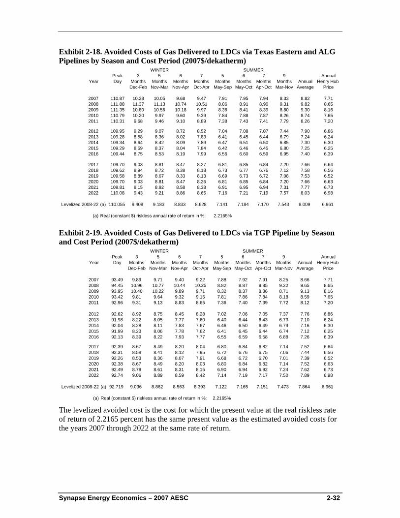
Synapse Energy Economics – 2007 AESC 2-32
Exhibit 2-18. Avoided Costs of Gas Delivered to LDCs via Texas Eastern and ALG Pipelines by Season and Cost Period (2007$/dekatherm)
Peak 3 5 6 7 5 6 7 9 AnnualYear Day Months Months Months Months Months Months Months Months Annual Henry Hub
Dec-Feb Nov-Mar Nov-Apr Oct-Apr May-Sep May-Oct Apr-Oct Mar-Nov Average Price
2007 110.87 10.28 10.05 9.68 9.47 7.91 7.95 7.94 8.33 8.82 7.712008 111.88 11.37 11.13 10.74 10.51 8.86 8.91 8.90 9.31 9.82 8.652009 111.35 10.80 10.56 10.18 9.97 8.36 8.41 8.39 8.80 9.30 8.162010 110.79 10.20 9.97 9.60 9.39 7.84 7.88 7.87 8.26 8.74 7.652011 110.31 9.68 9.46 9.10 8.89 7.38 7.43 7.41 7.79 8.26 7.20
2012 109.95 9.29 9.07 8.72 8.52 7.04 7.08 7.07 7.44 7.90 6.862013 109.28 8.58 8.36 8.02 7.83 6.41 6.45 6.44 6.79 7.24 6.242014 109.34 8.64 8.42 8.09 7.89 6.47 6.51 6.50 6.85 7.30 6.302015 109.29 8.59 8.37 8.04 7.84 6.42 6.46 6.45 6.80 7.25 6.252016 109.44 8.75 8.53 8.19 7.99 6.56 6.60 6.59 6.95 7.40 6.39
2017 109.70 9.03 8.81 8.47 8.27 6.81 6.85 6.84 7.20 7.66 6.642018 109.62 8.94 8.72 8.38 8.18 6.73 6.77 6.76 7.12 7.58 6.562019 109.58 8.89 8.67 8.33 8.13 6.69 6.73 6.72 7.08 7.53 6.522020 109.70 9.03 8.81 8.47 8.26 6.81 6.85 6.84 7.20 7.66 6.632021 109.81 9.15 8.92 8.58 8.38 6.91 6.95 6.94 7.31 7.77 6.732022 110.08 9.43 9.21 8.86 8.65 7.16 7.21 7.19 7.57 8.03 6.98
Levelized 2008-22 (a) 110.055 9.408 9.183 8.833 8.628 7.141 7.184 7.170 7.543 8.009 6.961
(a) Real (constant $) riskless annual rate of return in %: 2.2165%
WINTER SUMMER
Exhibit 2-19. Avoided Costs of Gas Delivered to LDCs via TGP Pipeline by Season and Cost Period (2007$/dekatherm)
Peak 3 5 6 7 5 6 7 9 AnnualYear Day Months Months Months Months Months Months Months Months Annual Henry Hub
Dec-Feb Nov-Mar Nov-Apr Oct-Apr May-Sep May-Oct Apr-Oct Mar-Nov Average Price
2007 93.49 9.89 9.71 9.40 9.22 7.88 7.92 7.91 8.25 8.66 7.712008 94.45 10.96 10.77 10.44 10.25 8.82 8.87 8.85 9.22 9.65 8.652009 93.95 10.40 10.22 9.89 9.71 8.32 8.37 8.36 8.71 9.13 8.162010 93.42 9.81 9.64 9.32 9.15 7.81 7.86 7.84 8.18 8.59 7.652011 92.96 9.31 9.13 8.83 8.65 7.36 7.40 7.39 7.72 8.12 7.20
2012 92.62 8.92 8.75 8.45 8.28 7.02 7.06 7.05 7.37 7.76 6.862013 91.98 8.22 8.05 7.77 7.60 6.40 6.44 6.43 6.73 7.10 6.242014 92.04 8.28 8.11 7.83 7.67 6.46 6.50 6.49 6.79 7.16 6.302015 91.99 8.23 8.06 7.78 7.62 6.41 6.45 6.44 6.74 7.12 6.252016 92.13 8.39 8.22 7.93 7.77 6.55 6.59 6.58 6.88 7.26 6.39
2017 92.39 8.67 8.49 8.20 8.04 6.80 6.84 6.82 7.14 7.52 6.642018 92.31 8.58 8.41 8.12 7.95 6.72 6.76 6.75 7.06 7.44 6.562019 92.26 8.53 8.36 8.07 7.91 6.68 6.72 6.70 7.01 7.39 6.522020 92.38 8.67 8.49 8.20 8.03 6.80 6.84 6.82 7.14 7.52 6.632021 92.49 8.78 8.61 8.31 8.15 6.90 6.94 6.92 7.24 7.62 6.732022 92.74 9.06 8.89 8.59 8.42 7.14 7.19 7.17 7.50 7.89 6.98
Levelized 2008-22 (a) 92.719 9.036 8.862 8.563 8.393 7.122 7.165 7.151 7.473 7.864 6.961
(a) Real (constant $) riskless annual rate of return in %: 2.2165%
WINTER SUMMER
The levelized avoided cost is the cost for which the present value at the real riskless rate of return of 2.2165 percent has the same present value as the estimated avoided costs for the years 2007 through 2022 at the same rate of return.
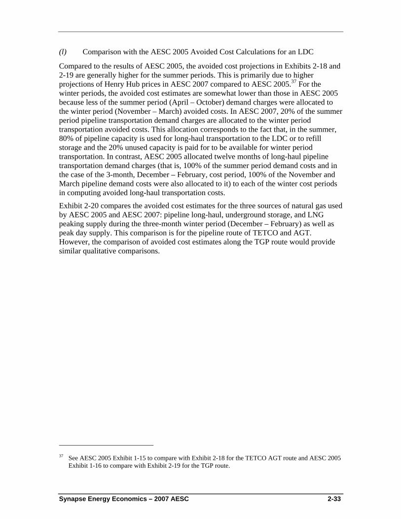
Synapse Energy Economics – 2007 AESC 2-33
(l) Comparison with the AESC 2005 Avoided Cost Calculations for an LDC
Compared to the results of AESC 2005, the avoided cost projections in Exhibits 2-18 and 2-19 are generally higher for the summer periods. This is primarily due to higher projections of Henry Hub prices in AESC 2007 compared to AESC 2005.37 For the winter periods, the avoided cost estimates are somewhat lower than those in AESC 2005 because less of the summer period (April – October) demand charges were allocated to the winter period (November – March) avoided costs. In AESC 2007, 20% of the summer period pipeline transportation demand charges are allocated to the winter period transportation avoided costs. This allocation corresponds to the fact that, in the summer, 80% of pipeline capacity is used for long-haul transportation to the LDC or to refill storage and the 20% unused capacity is paid for to be available for winter period transportation. In contrast, AESC 2005 allocated twelve months of long-haul pipeline transportation demand charges (that is, 100% of the summer period demand costs and in the case of the 3-month, December – February, cost period, 100% of the November and March pipeline demand costs were also allocated to it) to each of the winter cost periods in computing avoided long-haul transportation costs.
Exhibit 2-20 compares the avoided cost estimates for the three sources of natural gas used by AESC 2005 and AESC 2007: pipeline long-haul, underground storage, and LNG peaking supply during the three-month winter period (December – February) as well as peak day supply. This comparison is for the pipeline route of TETCO and AGT. However, the comparison of avoided cost estimates along the TGP route would provide similar qualitative comparisons.
37 See AESC 2005 Exhibit 1-15 to compare with Exhibit 2-18 for the TETCO AGT route and AESC 2005
Exhibit 1-16 to compare with Exhibit 2-19 for the TGP route.
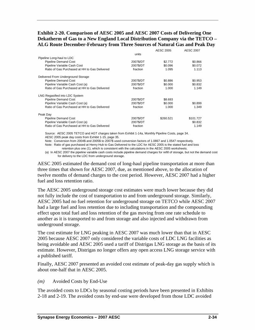
Synapse Energy Economics – 2007 AESC 2-34
Exhibit 2-20. Comparison of AESC 2005 and AESC 2007 Costs of Delivering One Dekatherm of Gas to a New England Local Distribution Company via the TETCO – ALG Route December-February from Three Sources of Natural Gas and Peak Day
AESC 2005 AESC 2007units
Pipeline Long-haul to LDCPipeline Demand Cost 2007$/DT $2.772 $0.866Pipeline Variable Cash Cost 2007$/DT $0.096 $0.072Ratio of Gas Purchased at HH to Gas Delivered fraction 1.095 1.113
Delivered From Underground StoragePipeline Demand Cost 2007$/DT $0.886 $0.953Pipeline Variable Cash Cost (a) 2007$/DT $0.000 $0.832Ratio of Gas Purchased at HH to Gas Delivered fraction 1.000 1.149
LNG Regasified into LDC SystemPipeline Demand Cost 2007$/DT $8.693Pipeline Variable Cash Cost (a) 2007$/DT $0.000 $0.899Ratio of Gas Purchased at HH to Gas Delivered fraction 1.000 1.349
Peak Day Pipeline Demand Cost 2007$/DT $260.521 $101.727Pipeline Variable Cash Cost (a) 2007$/DT $0.832Ratio of Gas Purchased at HH to Gas Delivered fraction 1.149
Source: AESC 2005 TETCO and AGT charges taken from Exhibit 1-14a, Monthly Pipeline Costs, page 34.AESC 2005 peak day costs from Exhibit 1-15, page 35.Note: Conversion from 2004$ and 2005$ to 2007$ used conversion factors of 1.0867 and 1.0547 respectively.Note: Ratio of gas purchased at Henry Hub to Gas Delivered to the LDC for AESC 2005 is the stated fuel and loss retention plus one (1), which is consistent with the calculations in the AESC 2005 worksheets.(a) In AESC 2007 the pipeline variable cash costs include pipeline demand charges for refill of storage, but not the demand costs for delivery to the LDC from underground storage.
AESC 2005 estimated the demand cost of long-haul pipeline transportation at more than three times that shown for AESC 2007, due, as mentioned above, to the allocation of twelve months of demand charges to the cost period. However, AESC 2007 had a higher fuel and loss retention ratio.
The AESC 2005 underground storage cost estimates were much lower because they did not fully include the cost of transportation to and from underground storage. Similarly, AESC 2005 had no fuel retention for underground storage on TETCO while AESC 2007 had a large fuel and loss retention due to including transportation and the compounding effect upon total fuel and loss retention of the gas moving from one rate schedule to another as it is transported to and from storage and also injected and withdrawn from underground storage.
The cost estimate for LNG peaking in AESC 2007 was much lower than that in AESC 2005 because AESC 2007 only considered the variable costs of LDC LNG facilities as being avoidable and AESC 2005 used a tariff of Distrigas LNG storage as the basis of its estimate. However, Distrigas no longer offers any open access LNG storage service with a published tariff.
Finally, AESC 2007 presented an avoided cost estimate of peak-day gas supply which is about one-half that in AESC 2005.
(m) Avoided Costs by End-Use
The avoided costs to LDCs by seasonal costing periods have been presented in Exhibits 2-18 and 2-19. The avoided costs by end-use were developed from those LDC avoided
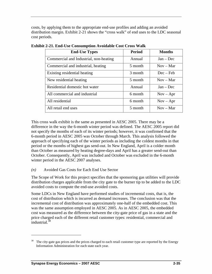
Synapse Energy Economics – 2007 AESC 2-35
costs, by applying them to the appropriate end-use profiles and adding an avoided distribution margin. Exhibit 2-21 shows the “cross walk” of end uses to the LDC seasonal cost periods.
Exhibit 2-21. End-Use Consumption Avoidable Cost Cross Walk End-Use Types Period Months
Commercial and Industrial, non-heating Annual Jan – Dec
Commercial and industrial, heating 5 month Nov – Mar
Existing residential heating 3 month Dec – Feb
New residential heating 5 month Nov – Mar
Residential domestic hot water Annual Jan – Dec
All commercial and industrial 6 month Nov – Apr
All residential 6 month Nov – Apr
All retail end uses 5 month Nov – Mar
This cross walk exhibit is the same as presented in AESC 2005. There may be a difference in the way the 6-month winter period was defined. The AESC 2005 report did not specify the months of each of its winter periods; however, it was confirmed that the 6-month period in AESC 2005 was October through March. This analysis followed the approach of specifying each of the winter periods as including the coldest months in that period or the months of highest gas send-out. In New England, April is a colder month than October as measured by heating degree-days and April has a greater send-out than October. Consequently, April was included and October was excluded in the 6-month winter period in the AESC 2007 analyses.
(n) Avoided Gas Costs for Each End Use Sector
The Scope of Work for this project specifies that the sponsoring gas utilities will provide distribution charges applicable from the city gate to the burner tip to be added to the LDC avoided costs to compute the end-use avoided costs.
Some LDCs in New England have performed studies of incremental costs, that is, the cost of distribution which is incurred as demand increases. The conclusion was that the incremental cost of distribution was approximately one-half of the embedded cost. This was the same assumption employed in AESC 2005. As in AESC 2005, the embedded cost was measured as the difference between the city-gate price of gas in a state and the price charged each of the different retail customer types: residential, commercial and industrial.38
38 The city-gate gas prices and the prices charged to each retail customer type are reported by the Energy
Information Administration for each state each year.
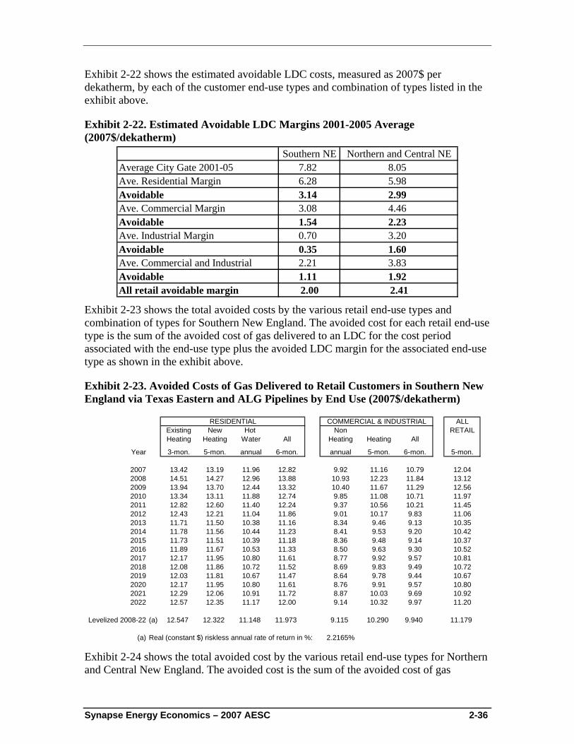
Synapse Energy Economics – 2007 AESC 2-36
Exhibit 2-22 shows the estimated avoidable LDC costs, measured as 2007$ per dekatherm, by each of the customer end-use types and combination of types listed in the exhibit above.
Exhibit 2-22. Estimated Avoidable LDC Margins 2001-2005 Average (2007$/dekatherm)
Southern NE Northern and Central NEAverage City Gate 2001-05 7.82 8.05Ave. Residential Margin 6.28 5.98Avoidable 3.14 2.99Ave. Commercial Margin 3.08 4.46Avoidable 1.54 2.23Ave. Industrial Margin 0.70 3.20Avoidable 0.35 1.60Ave. Commercial and Industrial 2.21 3.83Avoidable 1.11 1.92All retail avoidable margin 2.00 2.41
Exhibit 2-23 shows the total avoided costs by the various retail end-use types and combination of types for Southern New England. The avoided cost for each retail end-use type is the sum of the avoided cost of gas delivered to an LDC for the cost period associated with the end-use type plus the avoided LDC margin for the associated end-use type as shown in the exhibit above.
Exhibit 2-23. Avoided Costs of Gas Delivered to Retail Customers in Southern New England via Texas Eastern and ALG Pipelines by End Use (2007$/dekatherm)
ALLExisting New Hot Non RETAILHeating Heating Water All Heating Heating All
Year 3-mon. 5-mon. annual 6-mon. annual 5-mon. 6-mon. 5-mon.
2007 13.42 13.19 11.96 12.82 9.92 11.16 10.79 12.042008 14.51 14.27 12.96 13.88 10.93 12.23 11.84 13.122009 13.94 13.70 12.44 13.32 10.40 11.67 11.29 12.562010 13.34 13.11 11.88 12.74 9.85 11.08 10.71 11.972011 12.82 12.60 11.40 12.24 9.37 10.56 10.21 11.452012 12.43 12.21 11.04 11.86 9.01 10.17 9.83 11.062013 11.71 11.50 10.38 11.16 8.34 9.46 9.13 10.352014 11.78 11.56 10.44 11.23 8.41 9.53 9.20 10.422015 11.73 11.51 10.39 11.18 8.36 9.48 9.14 10.372016 11.89 11.67 10.53 11.33 8.50 9.63 9.30 10.522017 12.17 11.95 10.80 11.61 8.77 9.92 9.57 10.812018 12.08 11.86 10.72 11.52 8.69 9.83 9.49 10.722019 12.03 11.81 10.67 11.47 8.64 9.78 9.44 10.672020 12.17 11.95 10.80 11.61 8.76 9.91 9.57 10.802021 12.29 12.06 10.91 11.72 8.87 10.03 9.69 10.922022 12.57 12.35 11.17 12.00 9.14 10.32 9.97 11.20
Levelized 2008-22 (a) 12.547 12.322 11.148 11.973 9.115 10.290 9.940 11.179
(a) Real (constant $) riskless annual rate of return in %: 2.2165%
COMMERCIAL & INDUSTRIALRESIDENTIAL
Exhibit 2-24 shows the total avoided cost by the various retail end-use types for Northern and Central New England. The avoided cost is the sum of the avoided cost of gas
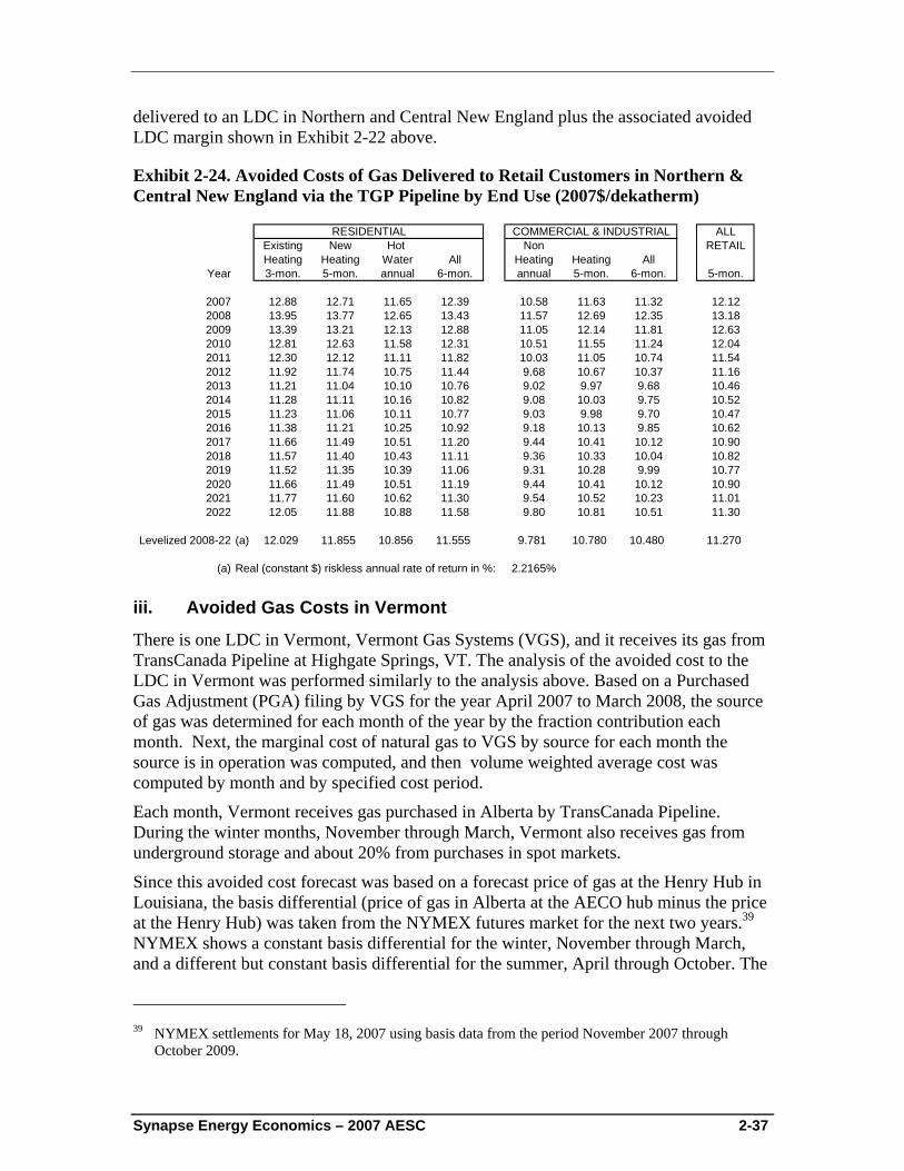
Synapse Energy Economics – 2007 AESC 2-37
delivered to an LDC in Northern and Central New England plus the associated avoided LDC margin shown in Exhibit 2-22 above.
Exhibit 2-24. Avoided Costs of Gas Delivered to Retail Customers in Northern & Central New England via the TGP Pipeline by End Use (2007$/dekatherm)
ALLExisting New Hot Non RETAILHeating Heating Water All Heating Heating All
Year 3-mon. 5-mon. annual 6-mon. annual 5-mon. 6-mon. 5-mon.
2007 12.88 12.71 11.65 12.39 10.58 11.63 11.32 12.122008 13.95 13.77 12.65 13.43 11.57 12.69 12.35 13.182009 13.39 13.21 12.13 12.88 11.05 12.14 11.81 12.632010 12.81 12.63 11.58 12.31 10.51 11.55 11.24 12.042011 12.30 12.12 11.11 11.82 10.03 11.05 10.74 11.542012 11.92 11.74 10.75 11.44 9.68 10.67 10.37 11.162013 11.21 11.04 10.10 10.76 9.02 9.97 9.68 10.462014 11.28 11.11 10.16 10.82 9.08 10.03 9.75 10.522015 11.23 11.06 10.11 10.77 9.03 9.98 9.70 10.472016 11.38 11.21 10.25 10.92 9.18 10.13 9.85 10.622017 11.66 11.49 10.51 11.20 9.44 10.41 10.12 10.902018 11.57 11.40 10.43 11.11 9.36 10.33 10.04 10.822019 11.52 11.35 10.39 11.06 9.31 10.28 9.99 10.772020 11.66 11.49 10.51 11.19 9.44 10.41 10.12 10.902021 11.77 11.60 10.62 11.30 9.54 10.52 10.23 11.012022 12.05 11.88 10.88 11.58 9.80 10.81 10.51 11.30
Levelized 2008-22 (a) 12.029 11.855 10.856 11.555 9.781 10.780 10.480 11.270
(a) Real (constant $) riskless annual rate of return in %: 2.2165%
RESIDENTIAL COMMERCIAL & INDUSTRIAL
iii. Avoided Gas Costs in Vermont
There is one LDC in Vermont, Vermont Gas Systems (VGS), and it receives its gas from TransCanada Pipeline at Highgate Springs, VT. The analysis of the avoided cost to the LDC in Vermont was performed similarly to the analysis above. Based on a Purchased Gas Adjustment (PGA) filing by VGS for the year April 2007 to March 2008, the source of gas was determined for each month of the year by the fraction contribution each month. Next, the marginal cost of natural gas to VGS by source for each month the source is in operation was computed, and then volume weighted average cost was computed by month and by specified cost period.
Each month, Vermont receives gas purchased in Alberta by TransCanada Pipeline. During the winter months, November through March, Vermont also receives gas from underground storage and about 20% from purchases in spot markets.
Since this avoided cost forecast was based on a forecast price of gas at the Henry Hub in Louisiana, the basis differential (price of gas in Alberta at the AECO hub minus the price at the Henry Hub) was taken from the NYMEX futures market for the next two years.39 NYMEX shows a constant basis differential for the winter, November through March, and a different but constant basis differential for the summer, April through October. The
39 NYMEX settlements for May 18, 2007 using basis data from the period November 2007 through
October 2009.
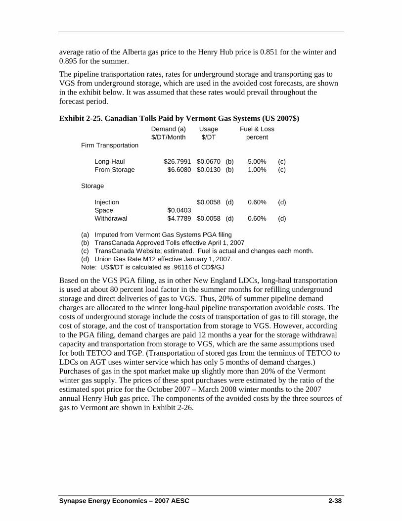
Synapse Energy Economics – 2007 AESC 2-38
average ratio of the Alberta gas price to the Henry Hub price is 0.851 for the winter and 0.895 for the summer.
The pipeline transportation rates, rates for underground storage and transporting gas to VGS from underground storage, which are used in the avoided cost forecasts, are shown in the exhibit below. It was assumed that these rates would prevail throughout the forecast period.
Exhibit 2-25. Canadian Tolls Paid by Vermont Gas Systems (US 2007$) Demand (a) Usage Fuel & Loss$/DT/Month $/DT percent
Firm Transportation
Long-Haul $26.7991 $0.0670 (b) 5.00% (c)From Storage $6.6080 $0.0130 (b) 1.00% (c)
Storage
Injection $0.0058 (d) 0.60% (d)Space $0.0403Withdrawal $4.7789 $0.0058 (d) 0.60% (d)
(a) Imputed from Vermont Gas Systems PGA filing(b) TransCanada Approved Tolls effective April 1, 2007(c) TransCanada Website; estimated. Fuel is actual and changes each month.(d) Union Gas Rate M12 effective January 1, 2007.Note: US$/DT is calculated as .96116 of CD$/GJ
Based on the VGS PGA filing, as in other New England LDCs, long-haul transportation is used at about 80 percent load factor in the summer months for refilling underground storage and direct deliveries of gas to VGS. Thus, 20% of summer pipeline demand charges are allocated to the winter long-haul pipeline transportation avoidable costs. The costs of underground storage include the costs of transportation of gas to fill storage, the cost of storage, and the cost of transportation from storage to VGS. However, according to the PGA filing, demand charges are paid 12 months a year for the storage withdrawal capacity and transportation from storage to VGS, which are the same assumptions used for both TETCO and TGP. (Transportation of stored gas from the terminus of TETCO to LDCs on AGT uses winter service which has only 5 months of demand charges.) Purchases of gas in the spot market make up slightly more than 20% of the Vermont winter gas supply. The prices of these spot purchases were estimated by the ratio of the estimated spot price for the October 2007 – March 2008 winter months to the 2007 annual Henry Hub gas price. The components of the avoided costs by the three sources of gas to Vermont are shown in Exhibit 2-26.
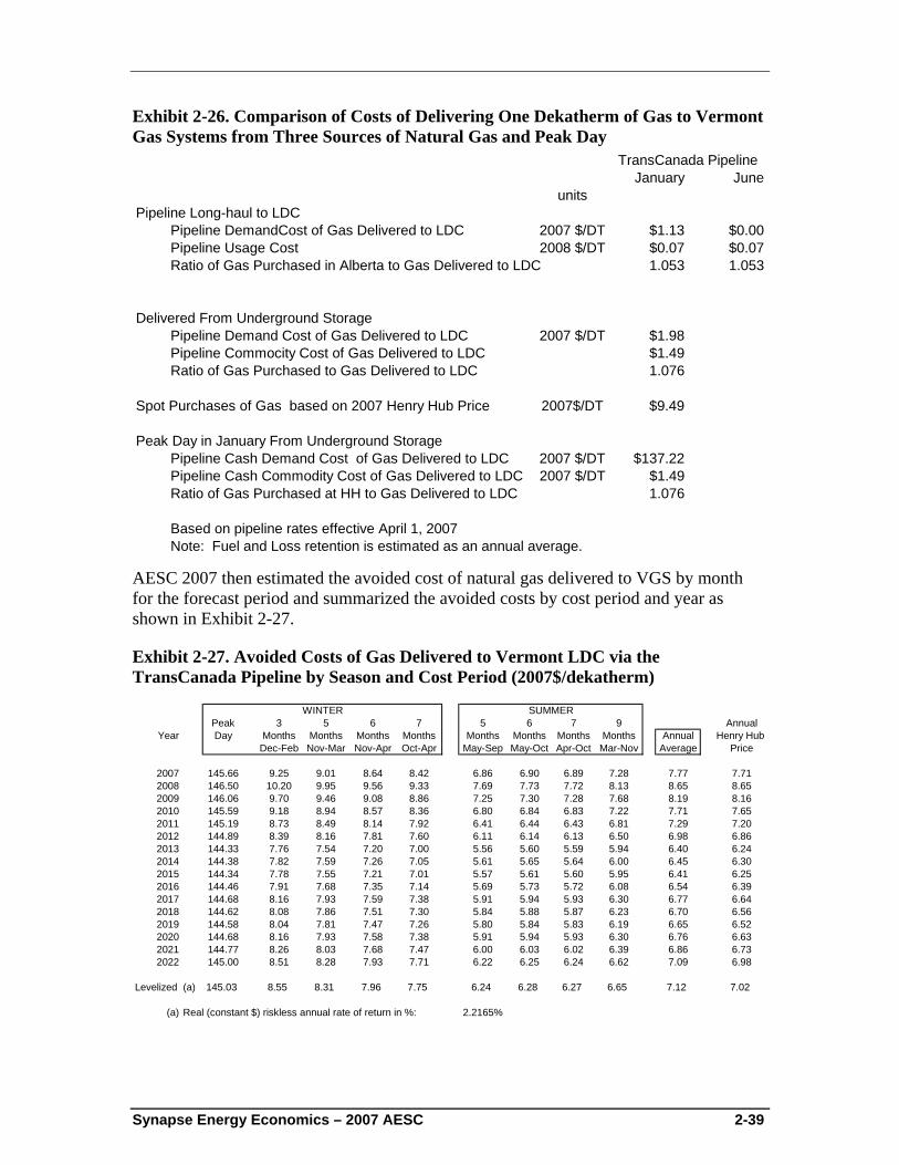
Synapse Energy Economics – 2007 AESC 2-39
Exhibit 2-26. Comparison of Costs of Delivering One Dekatherm of Gas to Vermont Gas Systems from Three Sources of Natural Gas and Peak Day
January Juneunits
Pipeline Long-haul to LDCPipeline DemandCost of Gas Delivered to LDC 2007 $/DT $1.13 $0.00Pipeline Usage Cost 2008 $/DT $0.07 $0.07Ratio of Gas Purchased in Alberta to Gas Delivered to LDC 1.053 1.053
Delivered From Underground StoragePipeline Demand Cost of Gas Delivered to LDC 2007 $/DT $1.98Pipeline Commocity Cost of Gas Delivered to LDC $1.49Ratio of Gas Purchased to Gas Delivered to LDC 1.076
Spot Purchases of Gas based on 2007 Henry Hub Price 2007$/DT $9.49
Peak Day in January From Underground StoragePipeline Cash Demand Cost of Gas Delivered to LDC 2007 $/DT $137.22Pipeline Cash Commodity Cost of Gas Delivered to LDC 2007 $/DT $1.49Ratio of Gas Purchased at HH to Gas Delivered to LDC 1.076
Based on pipeline rates effective April 1, 2007Note: Fuel and Loss retention is estimated as an annual average.
TransCanada Pipeline
AESC 2007 then estimated the avoided cost of natural gas delivered to VGS by month for the forecast period and summarized the avoided costs by cost period and year as shown in Exhibit 2-27.
Exhibit 2-27. Avoided Costs of Gas Delivered to Vermont LDC via the TransCanada Pipeline by Season and Cost Period (2007$/dekatherm)
Peak 3 5 6 7 5 6 7 9 AnnualYear Day Months Months Months Months Months Months Months Months Annual Henry Hub
Dec-Feb Nov-Mar Nov-Apr Oct-Apr May-Sep May-Oct Apr-Oct Mar-Nov Average Price
2007 145.66 9.25 9.01 8.64 8.42 6.86 6.90 6.89 7.28 7.77 7.712008 146.50 10.20 9.95 9.56 9.33 7.69 7.73 7.72 8.13 8.65 8.652009 146.06 9.70 9.46 9.08 8.86 7.25 7.30 7.28 7.68 8.19 8.162010 145.59 9.18 8.94 8.57 8.36 6.80 6.84 6.83 7.22 7.71 7.652011 145.19 8.73 8.49 8.14 7.92 6.41 6.44 6.43 6.81 7.29 7.202012 144.89 8.39 8.16 7.81 7.60 6.11 6.14 6.13 6.50 6.98 6.862013 144.33 7.76 7.54 7.20 7.00 5.56 5.60 5.59 5.94 6.40 6.242014 144.38 7.82 7.59 7.26 7.05 5.61 5.65 5.64 6.00 6.45 6.302015 144.34 7.78 7.55 7.21 7.01 5.57 5.61 5.60 5.95 6.41 6.252016 144.46 7.91 7.68 7.35 7.14 5.69 5.73 5.72 6.08 6.54 6.392017 144.68 8.16 7.93 7.59 7.38 5.91 5.94 5.93 6.30 6.77 6.642018 144.62 8.08 7.86 7.51 7.30 5.84 5.88 5.87 6.23 6.70 6.562019 144.58 8.04 7.81 7.47 7.26 5.80 5.84 5.83 6.19 6.65 6.522020 144.68 8.16 7.93 7.58 7.38 5.91 5.94 5.93 6.30 6.76 6.632021 144.77 8.26 8.03 7.68 7.47 6.00 6.03 6.02 6.39 6.86 6.732022 145.00 8.51 8.28 7.93 7.71 6.22 6.25 6.24 6.62 7.09 6.98
Levelized (a) 145.03 8.55 8.31 7.96 7.75 6.24 6.28 6.27 6.65 7.12 7.02
(a) Real (constant $) riskless annual rate of return in %: 2.2165%
WINTER SUMMER
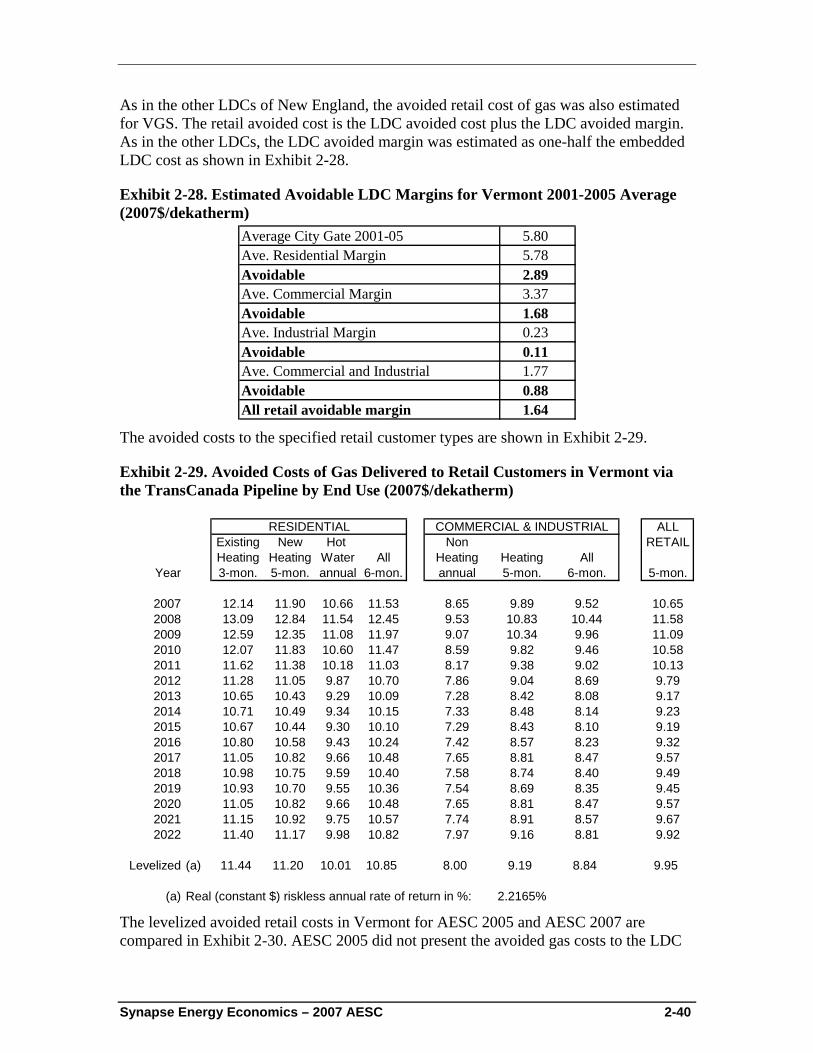
Synapse Energy Economics – 2007 AESC 2-40
As in the other LDCs of New England, the avoided retail cost of gas was also estimated for VGS. The retail avoided cost is the LDC avoided cost plus the LDC avoided margin. As in the other LDCs, the LDC avoided margin was estimated as one-half the embedded LDC cost as shown in Exhibit 2-28.
Exhibit 2-28. Estimated Avoidable LDC Margins for Vermont 2001-2005 Average (2007$/dekatherm)
Average City Gate 2001-05 5.80Ave. Residential Margin 5.78Avoidable 2.89Ave. Commercial Margin 3.37Avoidable 1.68Ave. Industrial Margin 0.23Avoidable 0.11Ave. Commercial and Industrial 1.77Avoidable 0.88All retail avoidable margin 1.64
The avoided costs to the specified retail customer types are shown in Exhibit 2-29.
Exhibit 2-29. Avoided Costs of Gas Delivered to Retail Customers in Vermont via the TransCanada Pipeline by End Use (2007$/dekatherm)
ALLExisting New Hot Non RETAILHeating Heating Water All Heating Heating All
Year 3-mon. 5-mon. annual 6-mon. annual 5-mon. 6-mon. 5-mon.
2007 12.14 11.90 10.66 11.53 8.65 9.89 9.52 10.652008 13.09 12.84 11.54 12.45 9.53 10.83 10.44 11.582009 12.59 12.35 11.08 11.97 9.07 10.34 9.96 11.092010 12.07 11.83 10.60 11.47 8.59 9.82 9.46 10.582011 11.62 11.38 10.18 11.03 8.17 9.38 9.02 10.132012 11.28 11.05 9.87 10.70 7.86 9.04 8.69 9.792013 10.65 10.43 9.29 10.09 7.28 8.42 8.08 9.172014 10.71 10.49 9.34 10.15 7.33 8.48 8.14 9.232015 10.67 10.44 9.30 10.10 7.29 8.43 8.10 9.192016 10.80 10.58 9.43 10.24 7.42 8.57 8.23 9.322017 11.05 10.82 9.66 10.48 7.65 8.81 8.47 9.572018 10.98 10.75 9.59 10.40 7.58 8.74 8.40 9.492019 10.93 10.70 9.55 10.36 7.54 8.69 8.35 9.452020 11.05 10.82 9.66 10.48 7.65 8.81 8.47 9.572021 11.15 10.92 9.75 10.57 7.74 8.91 8.57 9.672022 11.40 11.17 9.98 10.82 7.97 9.16 8.81 9.92
Levelized (a) 11.44 11.20 10.01 10.85 8.00 9.19 8.84 9.95
(a) Real (constant $) riskless annual rate of return in %: 2.2165%
RESIDENTIAL COMMERCIAL & INDUSTRIAL
The levelized avoided retail costs in Vermont for AESC 2005 and AESC 2007 are compared in Exhibit 2-30. AESC 2005 did not present the avoided gas costs to the LDC
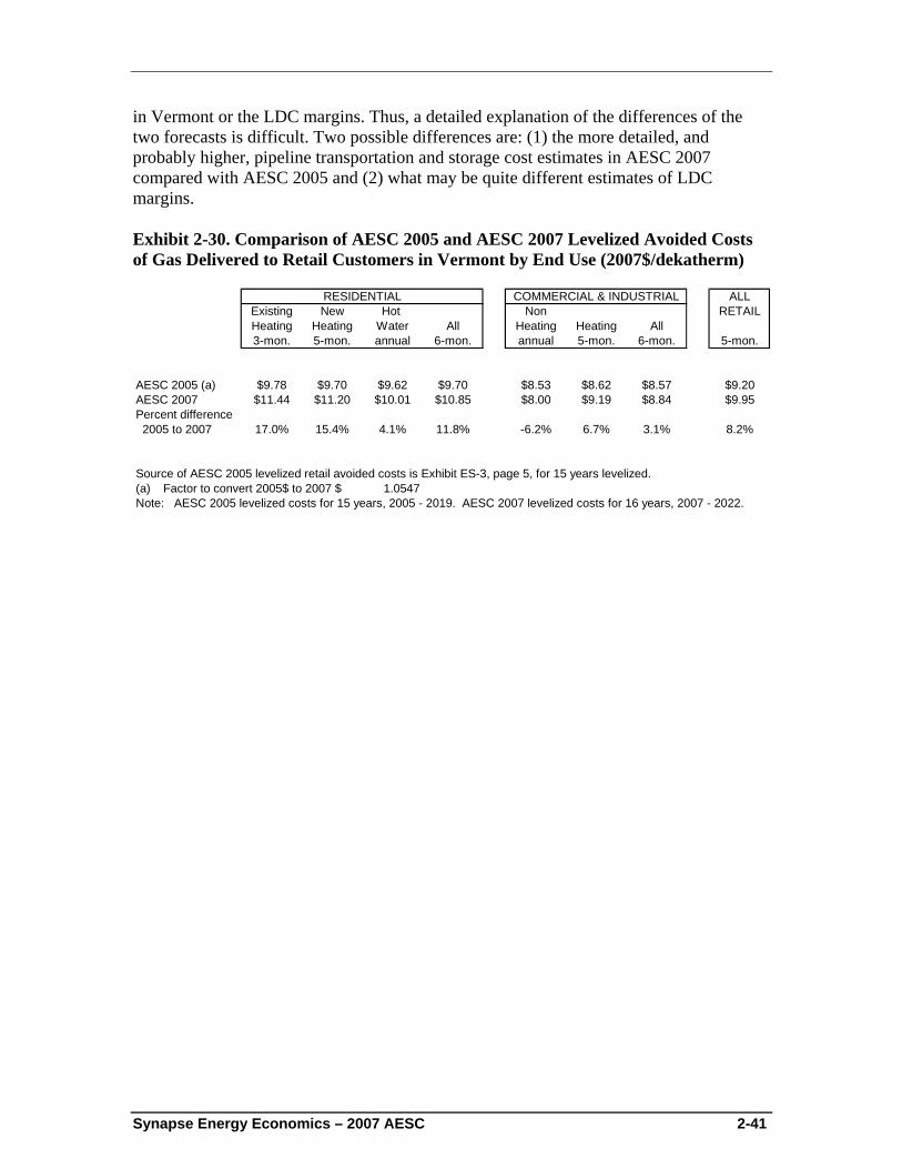
Synapse Energy Economics – 2007 AESC 2-41
in Vermont or the LDC margins. Thus, a detailed explanation of the differences of the two forecasts is difficult. Two possible differences are: (1) the more detailed, and probably higher, pipeline transportation and storage cost estimates in AESC 2007 compared with AESC 2005 and (2) what may be quite different estimates of LDC margins.
Exhibit 2-30. Comparison of AESC 2005 and AESC 2007 Levelized Avoided Costs of Gas Delivered to Retail Customers in Vermont by End Use (2007$/dekatherm)
ALLExisting New Hot Non RETAILHeating Heating Water All Heating Heating All3-mon. 5-mon. annual 6-mon. annual 5-mon. 6-mon. 5-mon.
AESC 2005 (a) $9.78 $9.70 $9.62 $9.70 $8.53 $8.62 $8.57 $9.20AESC 2007 $11.44 $11.20 $10.01 $10.85 $8.00 $9.19 $8.84 $9.95Percent difference 2005 to 2007 17.0% 15.4% 4.1% 11.8% -6.2% 6.7% 3.1% 8.2%
Source of AESC 2005 levelized retail avoided costs is Exhibit ES-3, page 5, for 15 years levelized.(a) Factor to convert 2005$ to 2007 $ 1.0547Note: AESC 2005 levelized costs for 15 years, 2005 - 2019. AESC 2007 levelized costs for 16 years, 2007 - 2022.
RESIDENTIAL COMMERCIAL & INDUSTRIAL
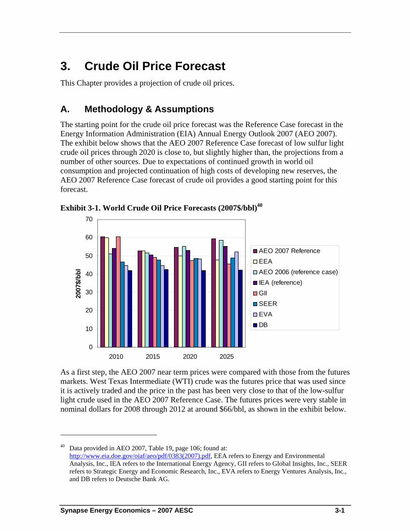
Synapse Energy Economics – 2007 AESC 3-1
3. Crude Oil Price Forecast This Chapter provides a projection of crude oil prices.
A. Methodology & Assumptions The starting point for the crude oil price forecast was the Reference Case forecast in the Energy Information Administration (EIA) Annual Energy Outlook 2007 (AEO 2007). The exhibit below shows that the AEO 2007 Reference Case forecast of low sulfur light crude oil prices through 2020 is close to, but slightly higher than, the projections from a number of other sources. Due to expectations of continued growth in world oil consumption and projected continuation of high costs of developing new reserves, the AEO 2007 Reference Case forecast of crude oil provides a good starting point for this forecast.
Exhibit 3-1. World Crude Oil Price Forecasts (2007$/bbl)40
0
10
20
30
40
50
60
70
2010 2015 2020 2025
2007
$/bb
l
AEO 2007 ReferenceEEAAEO 2006 (reference case)IEA (reference)GIISEEREVADB
As a first step, the AEO 2007 near term prices were compared with those from the futures markets. West Texas Intermediate (WTI) crude was the futures price that was used since it is actively traded and the price in the past has been very close to that of the low-sulfur light crude used in the AEO 2007 Reference Case. The futures prices were very stable in nominal dollars for 2008 through 2012 at around $66/bbl, as shown in the exhibit below.
40 Data provided in AEO 2007, Table 19, page 106; found at:
http://www.eia.doe.gov/oiaf/aeo/pdf/0383(2007).pdf, EEA refers to Energy and Environmental Analysis, Inc., IEA refers to the International Energy Agency, GII refers to Global Insights, Inc., SEER refers to Strategic Energy and Economic Research, Inc., EVA refers to Energy Ventures Analysis, Inc., and DB refers to Deutsche Bank AG.
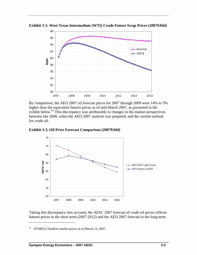
Synapse Energy Economics – 2007 AESC 3-2
Exhibit 3-2. West Texas Intermediate (WTI) Crude Future Swap Prices (2007$/bbl)
50
52
54
56
58
60
62
64
66
68
2007 2008 2009 2010 2011 2012 2013
$/bb
lNominal
2007$
By comparison, the AEO 2007 oil forecast prices for 2007 through 2009 were 14% to 3% higher than the equivalent futures prices as of mid-March 2007, as presented in the exhibit below.41 This discrepancy was attributable to changes in the market perspectives between late 2006, when the AEO 2007 analysis was prepared, and the current outlook for crude oil.
Exhibit 3-3. Oil Price Forecast Comparison (2007$/bbl)
40
45
50
55
60
65
70
75
2007 2008 2009 2010 2011 2012
2007
$ / b
bl
AEO 2007 Light Crude
WTI Futures 3/13/07
Taking this discrepancy into account, the AESC 2007 forecast of crude oil prices reflects futures prices in the short term (2007-2012) and the AEO 2007 forecast in the long-term 41 NYMEX ClearPort market prices as of March 13, 2007.
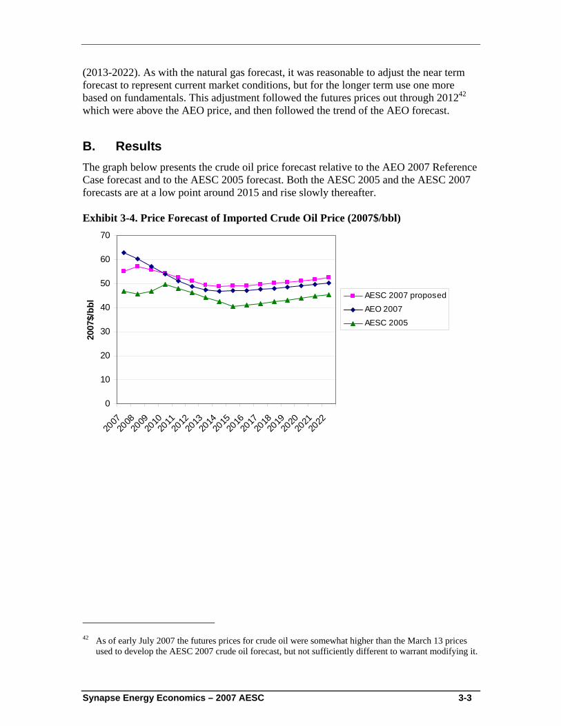
Synapse Energy Economics – 2007 AESC 3-3
(2013-2022). As with the natural gas forecast, it was reasonable to adjust the near term forecast to represent current market conditions, but for the longer term use one more based on fundamentals. This adjustment followed the futures prices out through 201242 which were above the AEO price, and then followed the trend of the AEO forecast.
B. Results The graph below presents the crude oil price forecast relative to the AEO 2007 Reference Case forecast and to the AESC 2005 forecast. Both the AESC 2005 and the AESC 2007 forecasts are at a low point around 2015 and rise slowly thereafter.
Exhibit 3-4. Price Forecast of Imported Crude Oil Price (2007$/bbl)
0
10
20
30
40
50
60
70
2007
2008
2009
2010
2011
2012
2013
2014
2015
2016
2017
2018
2019
2020
2021
2022
2007
$/bb
l AESC 2007 proposed
AEO 2007AESC 2005
42 As of early July 2007 the futures prices for crude oil were somewhat higher than the March 13 prices
used to develop the AESC 2007 crude oil forecast, but not sufficiently different to warrant modifying it.
Synapse Energy Economics – 2007 AESC 4-1
4. Forecasts of Other Fuel Prices This chapter provides a projection of fuel prices for electric generation as well as for retail end-use sector.
A. Methodology & Assumptions The starting point for the forecasts of other types of fuel oil, coal, and fuel wood prices was the Reference Case forecast in the Energy Information Administration (EIA) Annual Energy Outlook 2007 (AEO 2007). The Reference Case forecast of AEO 2007 provides forecasts for prices of residual fuel, distillate fuel, and coal used to generate electricity in New England. This forecast also provides projections of petroleum product prices for the residential, commercial and industrial sectors in New England.
The AESC 2007 forecasts of petroleum product prices were derived by adjusting the AEO petroleum product prices in proportion to the difference between the AEO crude oil and the AESC 2007 crude oil forecasts. This adjustment was made because petroleum product prices strongly reflect underlying crude oil prices. The AEO coal price forecasts were not adjusted.
To identify locational differences we analyzed the actual prices by sector by state from 1970 through 2004, which was the most recent historical data available from the EIA State Energy Data System (SEDS).43 SEDS is the most complete and consistent source of state-level energy prices. This review did not show consistent price differences between states for most products. There were two possible exceptions. One was for distillate fuel in New Hampshire, which for the last ten years has been about 6% below the New England average. The other was for residential prices for LPG which has been about 10% below the New England average for New Hampshire & Vermont, whereas for Rhode Island they have been about 15% above the average.
For commercial and industrial users the differences are much smaller and vary positive and negative from year to year. For years before 1995, the residential price differences between states were negligible and the relative rankings varied from year to year. Thus, the more recent retail locational price differences appear to be related to changes in the markups associated with competitive factors in the residential marketing and distribution systems in the various states. These differentials may or may not persist in the future. For this study, it was assumed that because of fundamentals, the end-use prices for all petroleum products across New England will be roughly the same. Thus, a single New England price by sector for the various oil-based products was recommended.44
The SEDS data for the five years 1999-2003 was also used to analyze the markups between petroleum product prices and crude oil prices. This analysis showed that the 43 http://www.eia.doe.gov/emeu/states/_seds.html 44 The AESC 2005 report had no differences in LPG costs between parts of New England. That report did
have differences in distillate oil prices that are not reflected in our analysis of the historic data.
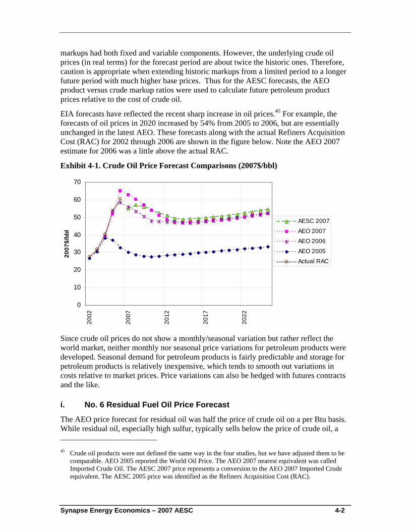
Synapse Energy Economics – 2007 AESC 4-2
markups had both fixed and variable components. However, the underlying crude oil prices (in real terms) for the forecast period are about twice the historic ones. Therefore, caution is appropriate when extending historic markups from a limited period to a longer future period with much higher base prices. Thus for the AESC forecasts, the AEO product versus crude markup ratios were used to calculate future petroleum product prices relative to the cost of crude oil.
EIA forecasts have reflected the recent sharp increase in oil prices.45 For example, the forecasts of oil prices in 2020 increased by 54% from 2005 to 2006, but are essentially unchanged in the latest AEO. These forecasts along with the actual Refiners Acquisition Cost (RAC) for 2002 through 2006 are shown in the figure below. Note the AEO 2007 estimate for 2006 was a little above the actual RAC.
Exhibit 4-1. Crude Oil Price Forecast Comparisons (2007$/bbl)
0
10
20
30
40
50
60
70
2002
2007
2012
2017
2022
2007
$/bb
l
AESC 2007
AEO 2007AEO 2006
AEO 2005Actual RAC
Since crude oil prices do not show a monthly/seasonal variation but rather reflect the world market, neither monthly nor seasonal price variations for petroleum products were developed. Seasonal demand for petroleum products is fairly predictable and storage for petroleum products is relatively inexpensive, which tends to smooth out variations in costs relative to market prices. Price variations can also be hedged with futures contracts and the like.
i. No. 6 Residual Fuel Oil Price Forecast
The AEO price forecast for residual oil was half the price of crude oil on a per Btu basis. While residual oil, especially high sulfur, typically sells below the price of crude oil, a 45 Crude oil products were not defined the same way in the four studies, but we have adjusted them to be
comparable. AEO 2005 reported the World Oil Price. The AEO 2007 nearest equivalent was called Imported Crude Oil. The AESC 2007 price represents a conversion to the AEO 2007 Imported Crude equivalent. The AESC 2005 price was identified as the Refiners Acquisition Cost (RAC).
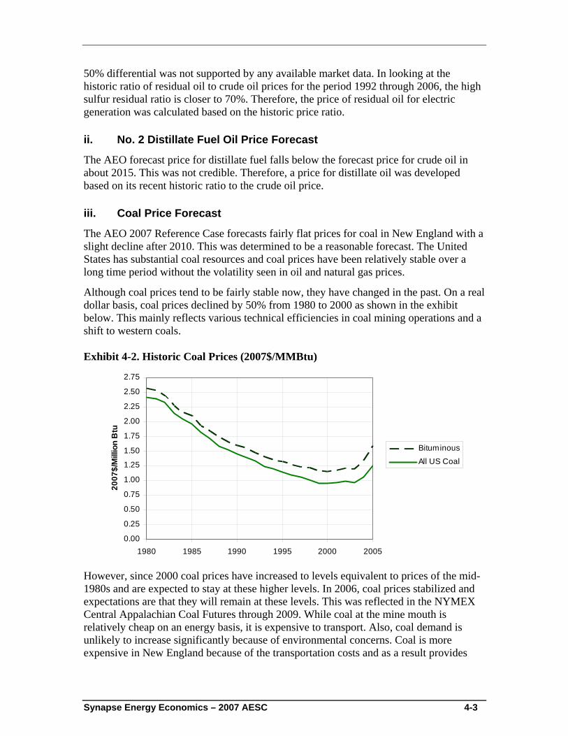
Synapse Energy Economics – 2007 AESC 4-3
50% differential was not supported by any available market data. In looking at the historic ratio of residual oil to crude oil prices for the period 1992 through 2006, the high sulfur residual ratio is closer to 70%. Therefore, the price of residual oil for electric generation was calculated based on the historic price ratio.
ii. No. 2 Distillate Fuel Oil Price Forecast
The AEO forecast price for distillate fuel falls below the forecast price for crude oil in about 2015. This was not credible. Therefore, a price for distillate oil was developed based on its recent historic ratio to the crude oil price.
iii. Coal Price Forecast
The AEO 2007 Reference Case forecasts fairly flat prices for coal in New England with a slight decline after 2010. This was determined to be a reasonable forecast. The United States has substantial coal resources and coal prices have been relatively stable over a long time period without the volatility seen in oil and natural gas prices.
Although coal prices tend to be fairly stable now, they have changed in the past. On a real dollar basis, coal prices declined by 50% from 1980 to 2000 as shown in the exhibit below. This mainly reflects various technical efficiencies in coal mining operations and a shift to western coals.
Exhibit 4-2. Historic Coal Prices (2007$/MMBtu)
0.00
0.25
0.50
0.75
1.00
1.25
1.50
1.75
2.00
2.25
2.50
2.75
1980 1985 1990 1995 2000 2005
2007
$/M
illio
n B
tu
Bituminous
All US Coal
However, since 2000 coal prices have increased to levels equivalent to prices of the mid-1980s and are expected to stay at these higher levels. In 2006, coal prices stabilized and expectations are that they will remain at these levels. This was reflected in the NYMEX Central Appalachian Coal Futures through 2009. While coal at the mine mouth is relatively cheap on an energy basis, it is expensive to transport. Also, coal demand is unlikely to increase significantly because of environmental concerns. Coal is more expensive in New England because of the transportation costs and as a result provides
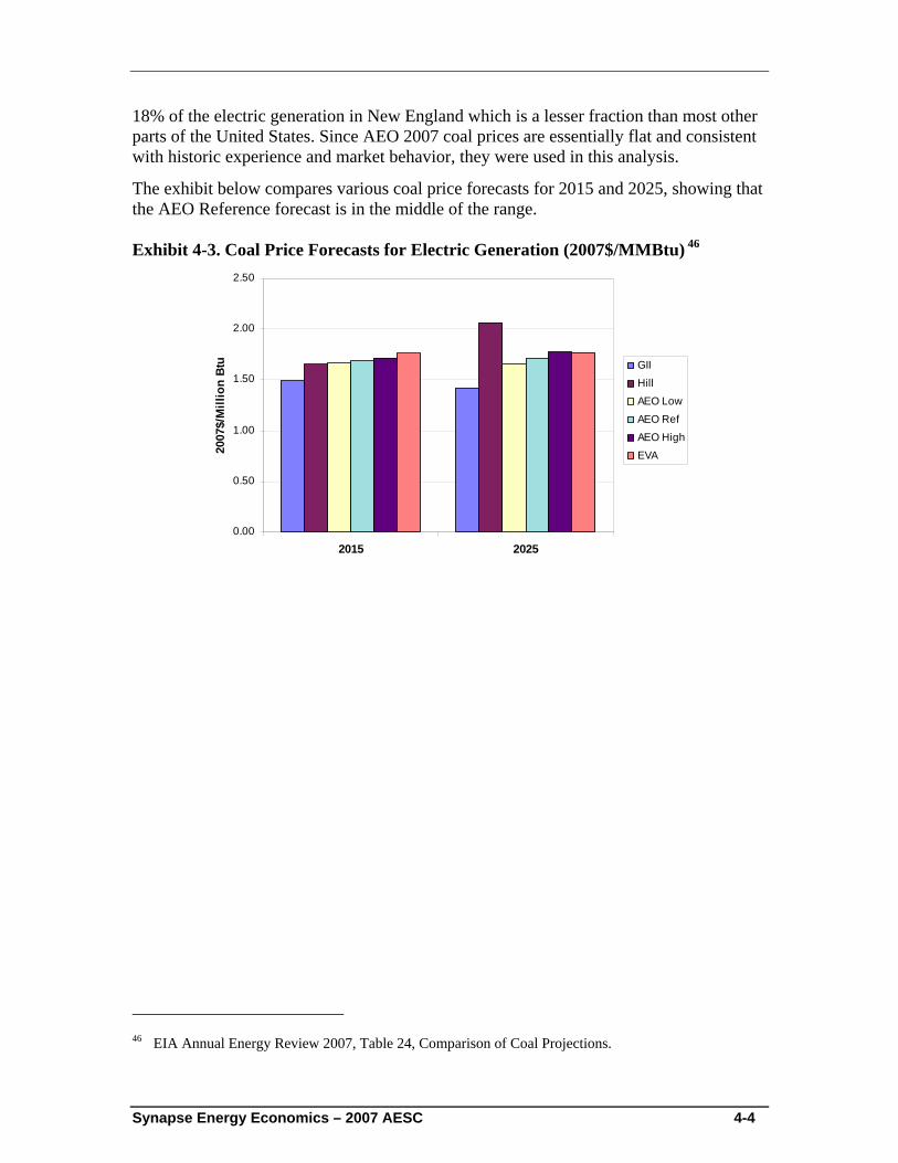
Synapse Energy Economics – 2007 AESC 4-4
18% of the electric generation in New England which is a lesser fraction than most other parts of the United States. Since AEO 2007 coal prices are essentially flat and consistent with historic experience and market behavior, they were used in this analysis.
The exhibit below compares various coal price forecasts for 2015 and 2025, showing that the AEO Reference forecast is in the middle of the range.
Exhibit 4-3. Coal Price Forecasts for Electric Generation (2007$/MMBtu) 46
0.00
0.50
1.00
1.50
2.00
2.50
2015 2025
2007
$/M
illio
n Bt
u GII
Hill
AEO Low
AEO Ref
AEO High
EVA
46 EIA Annual Energy Review 2007, Table 24, Comparison of Coal Projections.
Synapse Energy Economics – 2007 AESC 4-5
iv. Biofuel Price Forecasts
Biofuel blends are a mix of a petroleum product, such as No. 2 distillate oil or diesel, and an oil-like product derived from an agricultural source (e.g., soybeans). They are relatively new to New England and are being sold as heating fuels in competition with No. 2 distillate and as transportation fuels. These products are usually labeled “B”+“NN” where NN is the percent agricultural-derived component. Thus “B20” represents a product with a 20% bio component. The biofuel product of most interest is biodiesel. It is similar to No. 2 distillate fuel oil and used primarily for heating. Currently B20 is being sold as a heating oil product by Mass Energy at about a 9% premium to conventional heating oil on a per gallon basis. However, the biofuel heat content is about 2% greater, so the net premium is about 7%. A review of the relative national prices for biodiesel B20 compared to regular diesel from the DOE Alternative Fuels Data Center47 shows that on a heat rate basis the relative premium over the last year has varied from -1% to +3%. Since biofuels are both premium fuels (from an environmental standpoint) and sub-premium fuels (from a performance standpoint) and compete in a much larger market, an appropriate premium (positive or negative) to apply to their prices relative to the equivalent conventional fuel cannot be determined at this time. There is also the economic argument that the prices will equilibrate in the market. Thus, the prices of biofuels are forecast to be the same on an energy basis as the equivalent competitive fuel.
v. Fuel Wood Price Forecast
Prices for fuel wood can have great variability based on location, time of year, and quality (green or dry). A number of fuel wood dealers in New England were surveyed with the result being a wide range of prices. Additionally, it was very difficult to get any information from the dealers about historical prices or future price expectations.
As a result, historical data was leveraged. The EIA SEDS data provides state fuel wood prices by sector. In reviewing this data, there was a very strong and consistent relationship between distillate oil and fuel wood prices.
The following graph shows the historic relationship between No. 2 Distillate and fuel wood prices in Massachusetts from 1991 through 2003.48 The correlation between the two sets of prices is 99.4%. It is reasonable to conclude that this price relationship will continue into the future. As a result, the forecast for fuel wood prices was based on that for No. 2 Distillate.
47 “Clean Cities Alternative Fuel Price Report” for March 2007, October 2006, and June 2006.
www.eere.energy.gov/afdc/ 48 Massachusetts is the largest user of residential fuel wood in New England. The EIA data also reports
the same wood prices for all the New England states.
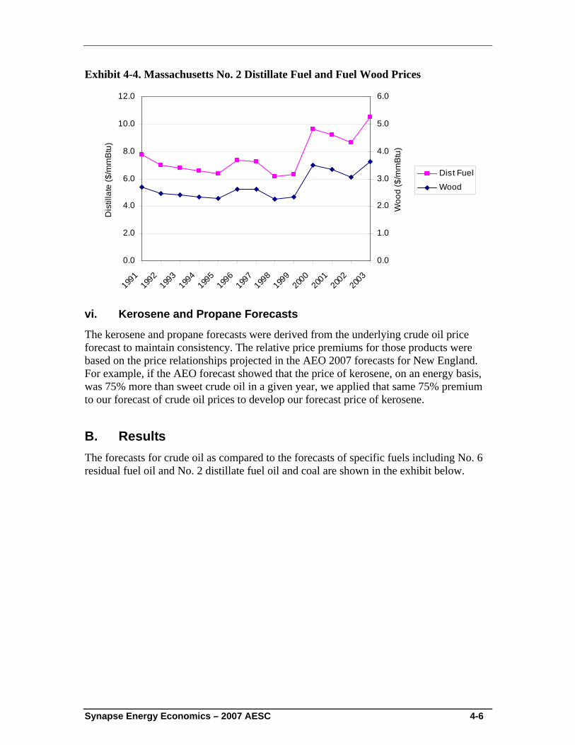
Synapse Energy Economics – 2007 AESC 4-6
Exhibit 4-4. Massachusetts No. 2 Distillate Fuel and Fuel Wood Prices
0.0
2.0
4.0
6.0
8.0
10.0
12.0
1991
1992
1993
1994
1995
1996
1997
1998
1999
2000
2001
2002
2003
Dis
tilla
te ($
/mm
Btu
)
0.0
1.0
2.0
3.0
4.0
5.0
6.0
Woo
d ($
/mm
Btu
)
Dist FuelWood
vi. Kerosene and Propane Forecasts
The kerosene and propane forecasts were derived from the underlying crude oil price forecast to maintain consistency. The relative price premiums for those products were based on the price relationships projected in the AEO 2007 forecasts for New England. For example, if the AEO forecast showed that the price of kerosene, on an energy basis, was 75% more than sweet crude oil in a given year, we applied that same 75% premium to our forecast of crude oil prices to develop our forecast price of kerosene.
B. Results The forecasts for crude oil as compared to the forecasts of specific fuels including No. 6 residual fuel oil and No. 2 distillate fuel oil and coal are shown in the exhibit below.
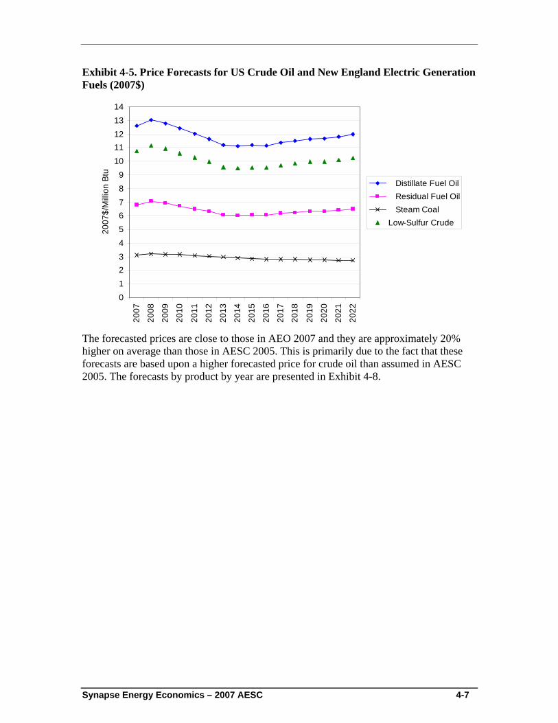
Synapse Energy Economics – 2007 AESC 4-7
Exhibit 4-5. Price Forecasts for US Crude Oil and New England Electric Generation Fuels (2007$)
0123456789
1011121314
2007
2008
2009
2010
2011
2012
2013
2014
2015
2016
2017
2018
2019
2020
2021
2022
2007
$/M
illion
Btu
Distillate Fuel Oil Residual Fuel Oil Steam CoalLow-Sulfur Crude
The forecasted prices are close to those in AEO 2007 and they are approximately 20% higher on average than those in AESC 2005. This is primarily due to the fact that these forecasts are based upon a higher forecasted price for crude oil than assumed in AESC 2005. The forecasts by product by year are presented in Exhibit 4-8.
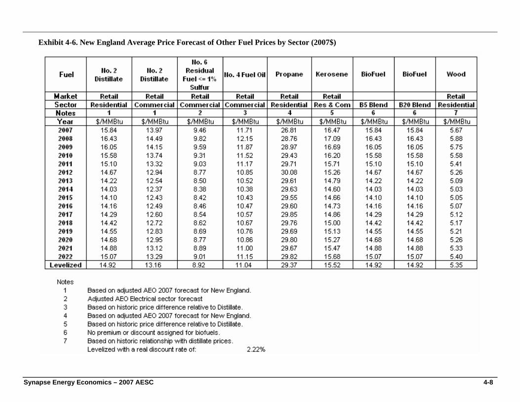
Synapse Energy Economics – 2007 AESC 4-8
Exhibit 4-6. New England Average Price Forecast of Other Fuel Prices by Sector (2007$)
Synapse Energy Economics – 2007 AESC 5-1
5. Electric Energy Price Forecast This chapter provides our projection of electric energy prices and a description of the modeling methodology and assumptions.
A. Overview The ISO New England market is part of the Northeast Power Coordinating Council (NPCC) and includes the states of Connecticut, Maine,49 Massachusetts, New Hampshire, Rhode Island, and Vermont. ISO New England, Inc. is the Regional Transmission Organization (RTO) for the New England power market and coordinates several markets for electric power products including energy, capacity, and operating reserves markets (Regulation Up and Down, spinning reserves, ten-minute non-spinning reserves, and thirty minute non-spinning reserves). This zonal locational marginal price-forecasting model (Market Analytics) simulates the operation of the energy and operating reserves markets, and produces forecasts of prices for each product. The model does not simulate the capacity market and, therefore, it does not require assumptions regarding the capital costs of new generation capacity, and the interconnection costs associated with such capacity. These assumptions were developed as part of the forecast of the prices for products in the capacity market and are discussed in the next section.
Market Analytics took as inputs the monthly regional fuel price forecasts reviewed in the first three sections (including the regional natural gas forecast and regional forecasts for petroleum products, coal and fuel wood). Other inputs as discussed in the Inputs section below were incorporated in order to produce an avoided electric energy cost forecast by state.
B. Zonal Locational Marginal Price-Forecasting Model The following section provides a high-level overview of the Global Energy Decisions (GED)50 EnerPrise Market Analytics data management and production simulation model functionality. The Market Analytics model was used to develop electricity avoided cost forecasts. Market Analytics uses the PROSYM simulation engine to produce optimized unit commitment and dispatch options. The model is a security-constrained chronological dispatch model that produces detailed and accurate results for hourly electricity prices and market operations.
The basic geographic unit in PROSYM is a sub region of a control area, called a “transmission area.” Transmission areas are defined in practice by actual transmission constraints within a control area. That is, power flows from one area to another in a control area are governed by the operational characteristics of the actual transmission
49 Parts of northeastern Maine are not included in ISO New England. 50 Formerly Henwood Energy Services, Inc.
Synapse Energy Economics – 2007 AESC 5-2
lines involved. New England, for example, consists of eleven transmission areas, including Southwest Connecticut as a zone. The service territories of the New England distribution utilities are mapped onto the transmission areas, and hourly load data is entered into PROSYM by distribution utility area. PROSYM can also simulate operation in any number of control areas. Groups of contiguous control areas were modeled in order to capture all regional impacts of the dynamics under scrutiny.
PROSYM uses highly detailed information on generating units. Data on specific units in the Market Analytics database are based on data drawn from various sources including the US Energy Information Administration (EIA), US Environmental Protection Agency (EPA), North American Electric Reliability Corporation (NERC), Federal Energy Regulatory Commission (FERC), and ISO New England databases as well as various trade press announcements and Global Energy’s own insight. Total existing capacity in the Market Analytics database was compared with the 2007 CELT report51 and found to be reasonably consistent.
For larger units, emission rates and operating characteristics are based on unit-specific data reported to EPA and EIA rather than on data based on unit type. Operating costs for each unit are based on plant-level operating costs reported to FERC and assessment of unit type and age. For smaller units (e.g., combustion turbines), most input data are based on unit type. All generating units in PROSYM operate at different heat rates (efficiencies) at different loading levels. This distinction is especially important in the case of combined-cycle units, which often operate in a simple-cycle mode at low loadings. PROSYM determines the fuel a unit burns by placing each generating unit into a “fuel group.” PROSYM does not limit the number of fuel groups used, and creating new fuel groups to simulate a few unusual units is a simple matter. In New England, for example, it is especially important to model the operation of dual-fueled units as accurately as possible.
Based upon hourly loads, PROSYM will determine generating unit commitment and operation by transmission zone based upon economic bid-based dispatch, subject to system operating procedures and constraints. PROSYM operates using hourly load data and simulates unit dispatch in chronological order. In other words, 8,760 distinct load levels are entered for each transmission area for each study year. The model begins on January 1st and dispatches generating units to meet load in each hour of the year. Using this chronological approach, PROSYM takes into account time-sensitive dynamics such as transmission constraints and operating characteristics of specific generating units. For example, one power plant might not be available at a given time due to its minimum down time (i.e., the period it must remain off line once it is taken off). Another unit might not be available to a given transmission area because of transmission constraints created by current operating conditions. These are dynamics that system operators wrestle with daily, and they often cause generating units to be dispatched out of merit order. Few other electric system models simulate dispatch in this kind of detail.
51 CELT is ISO-NE's annual 10-year forecast of capacity, energy, loads and transmission.
Synapse Energy Economics – 2007 AESC 5-3
The model’s fundamental assumption of behavior in competitive energy markets is that generators will bid their marginal cost of producing electric energy into the energy market. The model calculates this marginal cost from the unit’s opportunity cost of fuel52 or the spot price of gas at the location closest to the plant, variable operating and maintenance costs, and opportunity cost of tradable permits for air emissions.
PROSYM does not make capacity expansion decisions internally. Instead, the user specifies capacity additions, which increases transparency and allows the system expansion plans to be specified to reflect non-market considerations. PROSYM also models randomly occurring forced outages of generating units probabilistically rather than as deterministic capacity de-rating, thereby producing more accurate estimates of avoided costs, particular for peak load periods. PROSYM models generating units with a much higher level of detail including inputs for unit specific ramp rates, minimum up/down times, and multiple capacity blocks, all of which are critical for accurately modeling hourly prices. This modeling capability enabled production of locational prices by costing period in a consistent manner at the desired level of detail.
PROSYM simulates the effects of forced (i.e., random) outages probabilistically, using one of several Monte Carlo simulation modes. These simulation modes initiate forced outage events (full or partial) based on unit-specific outage probabilities and a Monte Carlo-type random number draw. Many other models simulate the effect of forced outages by “de-rating” the capacity of all generators within the system. That is, the capacities of all units are reduced at all times to simulate the outage of several units at any given time. While de-rating usually results in a reasonable estimate of the amount of annual generation from baseload plants, the result for intermediate and peaking units can be inaccurate, especially over short periods.
PROSYM calculates emissions of NOx, SO2, CO2, and mercury based on unit-specific emission rates. Emissions of other pollutants (e.g., particulates and air toxics) are calculated from emissions factors applied to fuel groups.
C. Input Assumptions Used to Develop the Electric Energy Price Forecast The avoided electric energy costs were strongly dependent on the quality of the input assumptions that were integrated into Global Energy’s zonal price forecasting model. The input assumptions include: topology, thermal unit characteristics, conventional hydro and pumped storage unit characteristics, renewable unit characteristics, hourly load profiles, forecasted annual peak demand and total energy, transmission system paths and upgrades, Reliability-Must-Run (RMR) Contracts, reserve margin multiplier, additions,
52 A number of generators have the ability to utilize a secondary fuel type. Units that are allowed to burn
gas or fuel oil are allowed to burn oil during the winter months (December, January, and February) and burn natural gas during the rest of the year. Fuel switching only occurs if oil is the less expensive option for these plants.
Synapse Energy Economics – 2007 AESC 5-4
retirements, uprates, outages, environmental regulations, demand response resources, marginal cost bidding, installed capacity, and ancillary services.
i. Electric Market Zone Topology
Market Analytics represents load and generation zones at various levels of aggregation. Assets within the Market Analytics model, including physical or contractual resources such as generators, transmission links, loads and transactions, are mapped to physical locations which are then mapped to Transmission Areas. Multiple Transmission Areas are linked by transmission paths to create Control Areas. For this study, New England is represented by 11 Transmission Areas that are based on the 13 load zones as defined by ISO New England for the 2006 Regional System Plan.53 Neighboring regions that are modeled in this study are New York, Quebec, and the Maritime Provinces.54 Areas outside of New England are represented with a high level of zonal aggregation to minimize model run time. The load and generation zones as they were modeled is presented in Exhibit 5-1.
53 Market Analytics combines western and central Maine/Saco Valley, New Hampshire and southeastern
Maine to form ME-CMP and includes Norwalk/Stamford in CT-SW. 54 The Maritimes zone includes Maine Public Service (MPS) and Eastern Maine Electric Cooperative
(EMEC) which are not part of ISO New England and, therefore, are not included in any of the New England pricing zones used in this study. MPS and EMEC are not modeled as part of the Maine pricing zone and were modeled as part of the New Brunswick transmission area. However, the forecast energy prices for the New Brunswick transmission area were on average within about 1% of the prices for the modeling zones included in the Maine pricing zone and MPS and EMEC constitute a small portion of Maine’s total load (approximately 6-7%). Market prices for standard-offer supply have been similar (considering the timing of procurement) among the three Maine utilities. Therefore, it is appropriate to apply the avoided costs for the Maine pricing zone to the entire state of Maine.
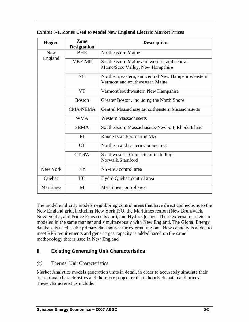
Synapse Energy Economics – 2007 AESC 5-5
Exhibit 5-1. Zones Used to Model New England Electric Market Prices
Region Zone Designation
Description
BHE Northeastern Maine
ME-CMP Southeastern Maine and western and central Maine/Saco Valley, New Hampshire
NH Northern, eastern, and central New Hampshire/eastern Vermont and southwestern Maine
VT Vermont/southwestern New Hampshire
Boston Greater Boston, including the North Shore
CMA/NEMA Central Massachusetts/northeastern Massachusetts
WMA Western Massachusetts
SEMA Southeastern Massachusetts/Newport, Rhode Island
RI Rhode Island/bordering MA
CT Northern and eastern Connecticut
New England
CT-SW Southwestern Connecticut including Norwalk/Stamford
New York NY NY-ISO control area
Quebec HQ Hydro Quebec control area
Maritimes M Maritimes control area
The model explicitly models neighboring control areas that have direct connections to the New England grid, including New York ISO, the Maritimes region (New Brunswick, Nova Scotia, and Prince Edwards Island), and Hydro Quebec. These external markets are modeled in the same manner and simultaneously with New England. The Global Energy database is used as the primary data source for external regions. New capacity is added to meet RPS requirements and generic gas capacity is added based on the same methodology that is used in New England.
ii. Existing Generating Unit Characteristics
(a) Thermal Unit Characteristics
Market Analytics models generation units in detail, in order to accurately simulate their operational characteristics and therefore project realistic hourly dispatch and prices. These characteristics include:
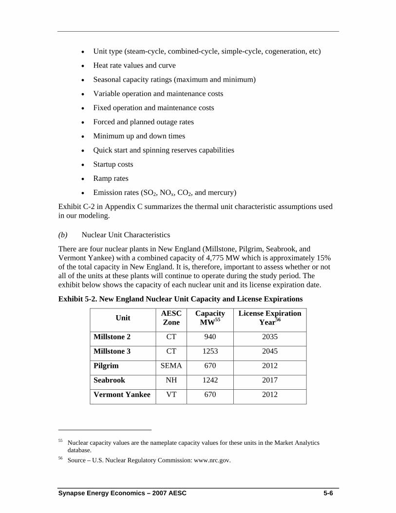
Synapse Energy Economics – 2007 AESC 5-6
• Unit type (steam-cycle, combined-cycle, simple-cycle, cogeneration, etc)
• Heat rate values and curve
• Seasonal capacity ratings (maximum and minimum)
• Variable operation and maintenance costs
• Fixed operation and maintenance costs
• Forced and planned outage rates
• Minimum up and down times
• Quick start and spinning reserves capabilities
• Startup costs
• Ramp rates
• Emission rates (SO2, NOx, CO2, and mercury)
Exhibit C-2 in Appendix C summarizes the thermal unit characteristic assumptions used in our modeling.
(b) Nuclear Unit Characteristics
There are four nuclear plants in New England (Millstone, Pilgrim, Seabrook, and Vermont Yankee) with a combined capacity of 4,775 MW which is approximately 15% of the total capacity in New England. It is, therefore, important to assess whether or not all of the units at these plants will continue to operate during the study period. The exhibit below shows the capacity of each nuclear unit and its license expiration date.
Exhibit 5-2. New England Nuclear Unit Capacity and License Expirations
Unit AESC Zone
Capacity MW55
License Expiration Year56
Millstone 2 CT 940 2035
Millstone 3 CT 1253 2045
Pilgrim SEMA 670 2012
Seabrook NH 1242 2017
Vermont Yankee VT 670 2012
55 Nuclear capacity values are the nameplate capacity values for these units in the Market Analytics
database. 56 Source – U.S. Nuclear Regulatory Commission: www.nrc.gov.
Synapse Energy Economics – 2007 AESC 5-7
License renewals for the Pilgrim and Vermont Yankee plants are currently being reviewed by the Nuclear Regulatory Commission (NRC) and Seabrook will be coming up for renewal during the study period. In the past seven years, the NRC has reviewed license extensions for 27 plants and not one of these applications was denied.57 Based on this track record and the lack of evidence that suggests that license renewal applications for any of these plants will be denied, it was assumed that all of the nuclear plants in New England will continue to operate for the entire study period.
The owners of Millstone have filed an application for a 70 MW uprate on Unit 3 for operation by the end of 2008.58 Based on the fact that the NRC has never denied an uprate application,59 it was assumed that this uprate will be approved and the uprated capacity will be in operation starting in 2009.
The maintenance schedules included in the Market Analytics database are based on information from the NRC website and the trade press for refueling outages as well as ISO New England and the Nuclear Energy Institute. Future outages are estimated by using typical refueling cycle, outage length, and last known outage dates of each plant to project refueling outages.
(c) Conventional Hydro and Pumped Storage Unit Characteristics
The Global Energy database was used as the primary source all hydro unit information. Conventional reservoir and run-of-river hydro resources are considered a “fixed energy” station or contract in the model. Like thermal stations, these stations have a maximum and minimum generating capacity, but they also have a fixed amount of energy available within a specified time (i.e., a week or a month). Hydro stations operate generally on peak in a manner that levels the load shape served by other stations. Hydro stations are scheduled one at a time over the horizon of a week, subject to hourly constraints for minimum and maximum generation, and weekly constraints for ramp rates and total energy. Although the load shape they intend to level is the overall system load, a hydro station can be scheduled against the load of a specified transmission area or control area.
Pumped-storage type resources (exchange contracts) have slightly different modeling requirements, typically involving a series of reservoirs used to release water for energy generation during peak load periods and pump water back uphill during off-peak times when energy demand and price is lower. The water (fuel) of pumped hydro generation is valued at the cost of pumping, allowing for net plant efficiency. Hourly reservoir levels are computed and a look-ahead is employed to prevent drawing the reservoir below the level where pumping space allows refilling to the desired level before the beginning of the next peak period.
57 Source – Nuclear Energy Institute:
http://www.nei.org/documents/U.S._Nuclear_License_Renewal_Filings.pdf 58 Source – ISO New England Generator Interconnection Queue 59 Source – U.S. Nuclear Regulatory Commission: www.nrc.gov.
Synapse Energy Economics – 2007 AESC 5-8
(d) Renewable Unit Characteristics
The Global Energy database includes several existing renewable generators in New England. These include wind, biomass, landfill gas, and municipal solid waste-to-energy facilities. All of these units were modeled as thermal units with seasonal forced outage rates that reflect historic seasonal capacity factor profiles.
iii. Load Forecast
Historical profiles for each utility were developed by Global Energy Decisions based on a set of annual historic load shapes. Hourly load profiles based on historical profiles were calculated for each load serving entity. Loads were then mapped to transmission areas based on location ratios.
Hourly load data for future years were scaled based on forecasted annual peak demand and total energy. Forecasted annual peak demand and total energy were derived from the 2007 CELT report and the 2006 Regional System Plan (RSP), published by ISO New England. The 2007 CELT report was released on April 18, 2007. However, the detailed load forecast data for the ISO’s RSP zones (which the Market Analytics zones are based on) was not released in time to be included in the modeling. Instead, the ISO released the load forecasts for each New England state that it had used to develop the forecast presented in the 2007 CELT.60 As a result, the load forecasts for each zone in the Market Analytics model were derived from the ISO-NE 2007 CELT state-level load forecasts for 2007-2016 as summarized in Exhibits 5-3 and 5-4. For 2017-2022, load in each zone is assumed to grow at the Compound Annual Growth Rate (CAGR) of the 2007-2016 period.61
60 Available on the ISO New England website:
http://www.isonewengland.com/committees/comm_wkgrps/prtcpnts_comm/pac/mtrls/2007/apr52007/revised_%20pac18_preliminary_rsp_load_forecast.xls.
61 In July we were advised that the forecast of peak demand and energy we used to develop our forecast of energy prices was not entirely consistent with the trends currently projected by the ISO for the last five years of the study, 2017 through 2022. The system load factor from 2017 through 2022 under the current ISO New England forecast is somewhat higher than that under the forecast we used, reflecting their assumption that air conditioning penetration will approach a saturation point after 2016. Our review indicates that our projection of energy prices is still reasonable despite the slight differences in system load factor from 2017 to 2022. Had we used a forecast with a system load factor consistent with that currently projected by the ISO, our projected energy prices in peak periods would have been somewhat lower, all else being equal. However, under such a load forecast the projected mix of capacity additions would likely have also been different, with less new, efficient CT and CC capacity added. That change in capacity mix would have resulted in higher projected energy prices. Thus, our review indicates that using a forecast with a somewhat higher system load factor from 2017 to 2022 would not result in materially different energy prices.
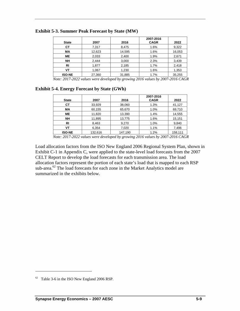
Synapse Energy Economics – 2007 AESC 5-9
Exhibit 5-3. Summer Peak Forecast by State (MW)
State 2007 2016 2007-2016
CAGR 2022 CT 7,317 8,475 1.6% 9,322 MA 12,623 14,595 1.6% 16,053 ME 2,033 2,400 1.9% 2,671 NH 2,444 3,000 2.3% 3,439 RI 1,877 2,185 1.7% 2,418 VT 1,067 1,230 1.6% 1,353
ISO-NE 27,360 31,885 1.7% 35,255 Note: 2017-2022 values were developed by growing 2016 values by 2007-2016 CAGR
Exhibit 5-4. Energy Forecast by State (GWh)
State 2007 2016 2007-2016
CAGR 2022 CT 33,929 38,060 1.3% 41,127 MA 60,155 65,670 1.0% 69,710 ME 11,820 13,390 1.4% 14,555 NH 11,895 13,775 1.6% 15,151 RI 8,463 9,270 1.0% 9,840 VT 6,354 7,020 1.1% 7,496
ISO-NE 132,616 147,190 1.2% 158,111 Note: 2017-2022 values were developed by growing 2016 values by 2007-2016 CAGR
Load allocation factors from the ISO New England 2006 Regional System Plan, shown in Exhibit C-1 in Appendix C, were applied to the state-level load forecasts from the 2007 CELT Report to develop the load forecasts for each transmission area. The load allocation factors represent the portion of each state’s load that is mapped to each RSP sub-area.62 The load forecasts for each zone in the Market Analytics model are summarized in the exhibits below.
62 Table 3-6 in the ISO New England 2006 RSP.
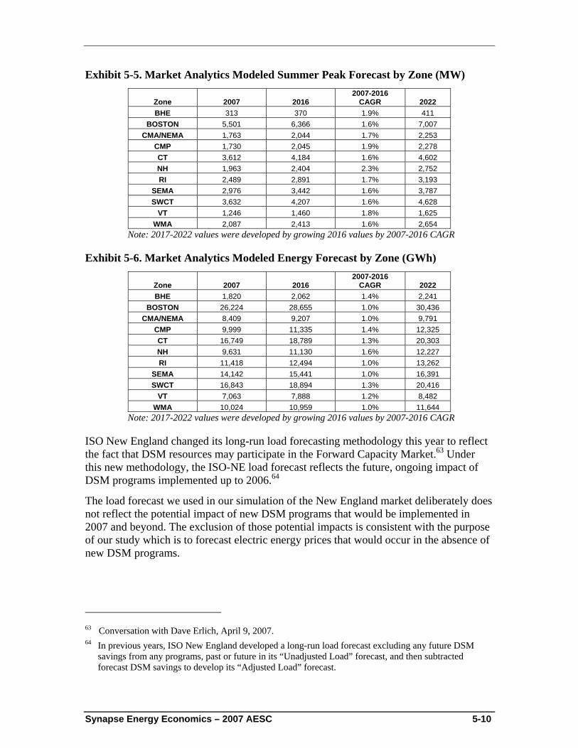
Synapse Energy Economics – 2007 AESC 5-10
Exhibit 5-5. Market Analytics Modeled Summer Peak Forecast by Zone (MW)
Zone 2007 2016 2007-2016
CAGR 2022 BHE 313 370 1.9% 411
BOSTON 5,501 6,366 1.6% 7,007 CMA/NEMA 1,763 2,044 1.7% 2,253
CMP 1,730 2,045 1.9% 2,278 CT 3,612 4,184 1.6% 4,602 NH 1,963 2,404 2.3% 2,752 RI 2,489 2,891 1.7% 3,193
SEMA 2,976 3,442 1.6% 3,787 SWCT 3,632 4,207 1.6% 4,628
VT 1,246 1,460 1.8% 1,625 WMA 2,087 2,413 1.6% 2,654
Note: 2017-2022 values were developed by growing 2016 values by 2007-2016 CAGR
Exhibit 5-6. Market Analytics Modeled Energy Forecast by Zone (GWh)
Zone 2007 2016 2007-2016
CAGR 2022 BHE 1,820 2,062 1.4% 2,241
BOSTON 26,224 28,655 1.0% 30,436 CMA/NEMA 8,409 9,207 1.0% 9,791
CMP 9,999 11,335 1.4% 12,325 CT 16,749 18,789 1.3% 20,303 NH 9,631 11,130 1.6% 12,227 RI 11,418 12,494 1.0% 13,262
SEMA 14,142 15,441 1.0% 16,391 SWCT 16,843 18,894 1.3% 20,416
VT 7,063 7,888 1.2% 8,482 WMA 10,024 10,959 1.0% 11,644
Note: 2017-2022 values were developed by growing 2016 values by 2007-2016 CAGR
ISO New England changed its long-run load forecasting methodology this year to reflect the fact that DSM resources may participate in the Forward Capacity Market.63 Under this new methodology, the ISO-NE load forecast reflects the future, ongoing impact of DSM programs implemented up to 2006.64
The load forecast we used in our simulation of the New England market deliberately does not reflect the potential impact of new DSM programs that would be implemented in 2007 and beyond. The exclusion of those potential impacts is consistent with the purpose of our study which is to forecast electric energy prices that would occur in the absence of new DSM programs.
63 Conversation with Dave Erlich, April 9, 2007. 64 In previous years, ISO New England developed a long-run load forecast excluding any future DSM
savings from any programs, past or future in its “Unadjusted Load” forecast, and then subtracted forecast DSM savings to develop its “Adjusted Load” forecast.
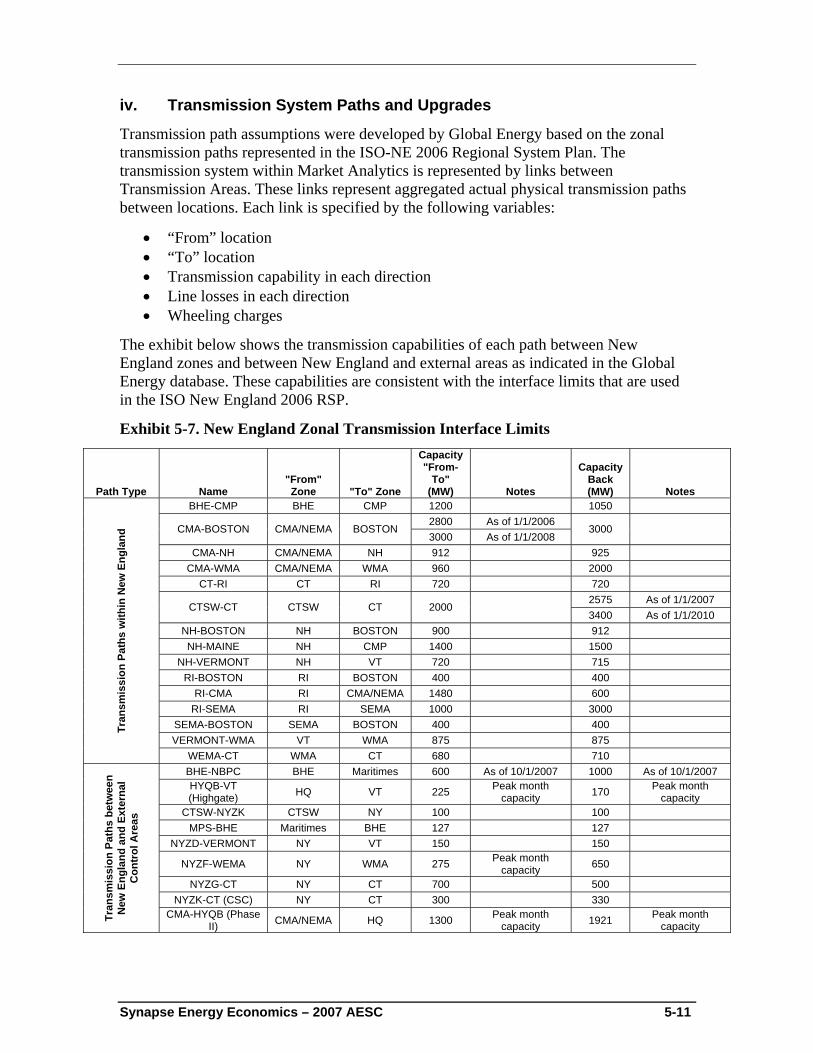
Synapse Energy Economics – 2007 AESC 5-11
iv. Transmission System Paths and Upgrades
Transmission path assumptions were developed by Global Energy based on the zonal transmission paths represented in the ISO-NE 2006 Regional System Plan. The transmission system within Market Analytics is represented by links between Transmission Areas. These links represent aggregated actual physical transmission paths between locations. Each link is specified by the following variables:
• “From” location • “To” location • Transmission capability in each direction • Line losses in each direction • Wheeling charges
The exhibit below shows the transmission capabilities of each path between New England zones and between New England and external areas as indicated in the Global Energy database. These capabilities are consistent with the interface limits that are used in the ISO New England 2006 RSP.
Exhibit 5-7. New England Zonal Transmission Interface Limits
Path Type Name "From" Zone "To" Zone
Capacity "From-
To" (MW) Notes
Capacity Back (MW) Notes
BHE-CMP BHE CMP 1200 1050 2800 As of 1/1/2006
CMA-BOSTON CMA/NEMA BOSTON 3000 As of 1/1/2008
3000
CMA-NH CMA/NEMA NH 912 925 CMA-WMA CMA/NEMA WMA 960 2000
CT-RI CT RI 720 720 2575 As of 1/1/2007
CTSW-CT CTSW CT 2000 3400 As of 1/1/2010
NH-BOSTON NH BOSTON 900 912 NH-MAINE NH CMP 1400 1500
NH-VERMONT NH VT 720 715 RI-BOSTON RI BOSTON 400 400
RI-CMA RI CMA/NEMA 1480 600 RI-SEMA RI SEMA 1000 3000
SEMA-BOSTON SEMA BOSTON 400 400 VERMONT-WMA VT WMA 875 875
Tran
smis
sion
Pat
hs w
ithin
New
Eng
land
WEMA-CT WMA CT 680 710 BHE-NBPC BHE Maritimes 600 As of 10/1/2007 1000 As of 10/1/2007 HYQB-VT (Highgate) HQ VT 225 Peak month
capacity 170 Peak month capacity
CTSW-NYZK CTSW NY 100 100 MPS-BHE Maritimes BHE 127 127
NYZD-VERMONT NY VT 150 150
NYZF-WEMA NY WMA 275 Peak month capacity 650
NYZG-CT NY CT 700 500 NYZK-CT (CSC) NY CT 300 330
Tran
smis
sion
Pat
hs b
etw
een
New
Eng
land
and
Ext
erna
l C
ontr
ol A
reas
CMA-HYQB (Phase II) CMA/NEMA HQ 1300 Peak month
capacity 1921 Peak month capacity
Synapse Energy Economics – 2007 AESC 5-12
The interface limits presented in the exhibit above include the following transmission upgrades from the 2006 RSP:65
• Northeast Reliability Interconnect Project – this comprises a new 345 kV line from New Brunswick to the Orrington Substation in northern Maine and increases the transfer capability from New Brunswick to Maine by 300 MW. This project is scheduled to be online by the end of 2007.
• NSTAR 345 kV Transmission Reliability Project – this project involves construction of a Stoughton 345 kV station and three new underground 345 kV lines, two of which are already completed and the third is scheduled for completion by the end of 2007. This project increases the Boston import capability by approximately 1,000 MW.
• SWCT Reliability Project – this project includes two phases of new 345 kV circuits. The combined effect of these two phases is to increase the import capability into Southwest Connecticut by approximately 1,100 MW by the end of 2009.
Transmission system upgrades beyond what was included in the Global Energy database were considered; however, no additional upgrades needed to be included.
v. Reliability-Must-Run (RMR) Contracts
Unlike the 2005 AESC study, the current study does not consider any costs related to existing reliability contracts (sometimes called “reliability must-run” or RMR contracts) as being avoidable. Exhibit 5-8 lists the plants with reliability agreements that last beyond 2007.66 These remaining reliability contracts are scheduled to expire in June 2010 when the FCM commences operation. Load reductions are unlikely to result in these contracts being avoided prior to 2010. Prior to 2010 we assume that these units will be needed. Based on that assumption, if the revenues these units receive from their market sales were to decline due to load reductions to the point that they were not covering their costs, we expect that ISO-NE would simply initiate new agreements and collect the revenue shortfall from New England customers.
65 The Northwest Vermont Reliability Project is not included in this list because it does not affect the
import capability into Vermont. 66 “Reliability Agreements – Annual Fixed Costs Summary,” ISO-NE, April 19, 2007.
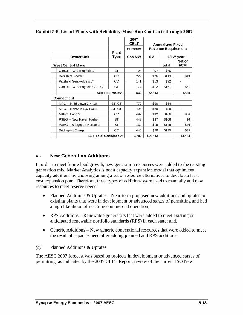
Synapse Energy Economics – 2007 AESC 5-13
Exhibit 5-8. List of Plants with Reliability-Must-Run Contracts through 2007
2007 CELT
Summer Annualized Fixed
Revenue Requirement
Owner/Unit Plant Type Cap MW $M $/kW-year
West Central Mass total Net of FCM
ConEd -- W.Springfield 3 ST 94 $7 $75 - Berkshire Power CC 229 $26 $113 $13 Pittsfield Gen.--Altresco" CC 141 $13 $92 -
ConEd -- W.Springfield GT-1&2 CT 74 $12 $161 $61
Sub-Total WCMA 539 $58 M $8 M
Connecticut NRG -- Middletown 2-4, 10 ST, CT 770 $50 $64 - NRG -- Montville 5,6,10&11 ST, CT 494 $29 $58 - Milford 1 and 2 CC 492 $82 $166 $66 PSEG -- New Haven Harbor ST 448 $47 $106 $6 PSEG -- Bridgeport Harbor 2 ST 130 $19 $146 $46
Bridgeport Energy CC 448 $58 $129 $29
Sub-Total Connecticut 2,782 $284 M $54 M
vi. New Generation Additions
In order to meet future load growth, new generation resources were added to the existing generation mix. Market Analytics is not a capacity expansion model that optimizes capacity additions by choosing among a set of resource alternatives to develop a least cost expansion plan. Therefore, three types of additions were used to manually add new resources to meet reserve needs:
• Planned Additions & Uprates – Near-term proposed new additions and uprates to existing plants that were in development or advanced stages of permitting and had a high likelihood of reaching commercial operation;
• RPS Additions – Renewable generators that were added to meet existing or anticipated renewable portfolio standards (RPS) in each state; and,
• Generic Additions – New generic conventional resources that were added to meet the residual capacity need after adding planned and RPS additions.
(a) Planned Additions & Uprates
The AESC 2007 forecast was based on projects in development or advanced stages of permitting, as indicated by the 2007 CELT Report, review of the current ISO New
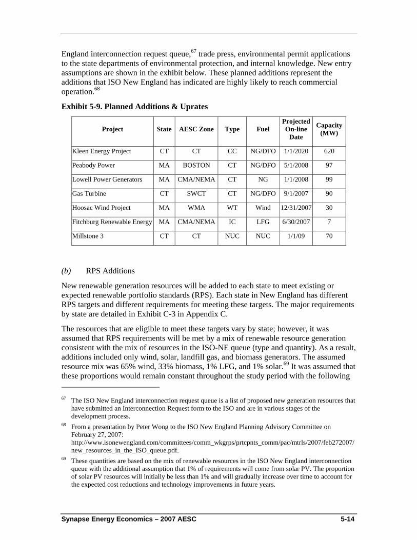
Synapse Energy Economics – 2007 AESC 5-14
England interconnection request queue,67 trade press, environmental permit applications to the state departments of environmental protection, and internal knowledge. New entry assumptions are shown in the exhibit below. These planned additions represent the additions that ISO New England has indicated are highly likely to reach commercial operation.68
Exhibit 5-9. Planned Additions & Uprates
Project State AESC Zone Type Fuel Projected On-line
Date
Capacity (MW)
Kleen Energy Project CT CT CC NG/DFO 1/1/2020 620
Peabody Power MA BOSTON CT NG/DFO 5/1/2008 97
Lowell Power Generators MA CMA/NEMA CT NG 1/1/2008 99
Gas Turbine CT SWCT CT NG/DFO 9/1/2007 90
Hoosac Wind Project MA WMA WT Wind 12/31/2007 30
Fitchburg Renewable Energy MA CMA/NEMA IC LFG 6/30/2007 7
Millstone 3 CT CT NUC NUC 1/1/09 70
(b) RPS Additions
New renewable generation resources will be added to each state to meet existing or expected renewable portfolio standards (RPS). Each state in New England has different RPS targets and different requirements for meeting these targets. The major requirements by state are detailed in Exhibit C-3 in Appendix C.
The resources that are eligible to meet these targets vary by state; however, it was assumed that RPS requirements will be met by a mix of renewable resource generation consistent with the mix of resources in the ISO-NE queue (type and quantity). As a result, additions included only wind, solar, landfill gas, and biomass generators. The assumed resource mix was 65% wind, 33% biomass, 1% LFG, and 1% solar.69 It was assumed that these proportions would remain constant throughout the study period with the following 67 The ISO New England interconnection request queue is a list of proposed new generation resources that
have submitted an Interconnection Request form to the ISO and are in various stages of the development process.
68 From a presentation by Peter Wong to the ISO New England Planning Advisory Committee on February 27, 2007: http://www.isonewengland.com/committees/comm_wkgrps/prtcpnts_comm/pac/mtrls/2007/feb272007/new_resources_in_the_ISO_queue.pdf.
69 These quantities are based on the mix of renewable resources in the ISO New England interconnection queue with the additional assumption that 1% of requirements will come from solar PV. The proportion of solar PV resources will initially be less than 1% and will gradually increase over time to account for the expected cost reductions and technology improvements in future years.
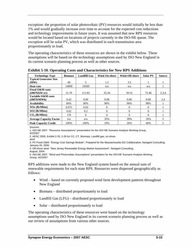
Synapse Energy Economics – 2007 AESC 5-15
exception: the proportion of solar photovoltaic (PV) resources would initially be less than 1% and would gradually increase over time to account for the expected cost reductions and technology improvements in future years. It was assumed that new RPS resources would be located based on locations of projects currently in the ISO-NE queue. The exception will be solar PV, which was distributed in each transmission area proportionately to load.
The operating characteristics of these resources are shown in the exhibit below. These assumptions will be based on the technology assumptions used by ISO New England in its current scenario planning process as well as other sources.
Exhibit 5-10. Operating Costs and Characteristics for New RPS Additions Technology Type Biomass Landfill Gas Wind On-shore Wind Off-shore Solar PV Source
Typical Generator Size (MW) 40 5 1.5 3.5 1 1 Heat rate 14000 10500 n/a n/a n/a 1 Fixed O&M costs (2007$/kW-yr) 51.70 111.83 35.34 50.31 72.46 2,3,4 Variable O&M costs (2007$/MWh) 0.42 0.00 0.00 0.00 0.00 2,4 Availability 60% 90% 90% 90% 98% 1 NOx (lb/Mbtu) 0.075 0.03 0 0 0 1 SO2 (lb/Mbtu) 0.02 0.2 0 0 0 1 CO2 (lb/Mbtu) 170 0 0 0 0 1 Average Capacity Factor n/a n/a 35% 39% 16% 5 Peak Capacity Credit 100% 100% 19% 26% 40% 5 Sources: 1. ISO-NE 2007. "Resource Assumptions" presentation for the ISO-NE Scenario Analysis Working Group, 4/2/2007 2. AESC 2005, Exhibit 2-25, 2-26 for CC, CT, Biomass, Landfill gas, on-shore wind 3. PV Fixed O&M: "Energy Cost Savings Module", Prepared for the Massachusetts DG Collaborative, Navigant Consulting, January 20, 2006. 4. Off-shore wind: "New Jersey Renewable Energy Market Assessment", Navigant Consulting, August, 2004. 5. ISO-NE 2007. "Wind and Photovoltaic Assumptions" presentation for the ISO-NE Scenario Analysis Working Group, 4/2/2007
RPS additions were made to the New England system based on the annual sum of renewable requirements for each state RPS. Resources were dispersed geographically as follows:
• Wind – based on currently proposed wind farm development patterns throughout New England
• Biomass – distributed proportionately to load
• Landfill Gas (LFG) – distributed proportionately to load
• Solar – distributed proportionately to load
The operating characteristics of these resources were based on the technology assumptions used by ISO New England in its current scenario planning process as well as our review of assumptions from various other sources.
Synapse Energy Economics – 2007 AESC 5-16
(c) Generic Additions
In order to reliably serve the forecasted load in the mid- to long-term portion of the forecast period, new generic additions were added to the model. A range of generation technologies was initially considered for this purpose, including gas/oil-fired combined-cycle, gas/oil combustion turbines, conventional coal, integrated gasification combined cycle (IGCC), and nuclear. However, the development queue did not indicate that any coal or nuclear resources would be developed in New England during the forecast period. Although the region is already heavily reliant on gas-fired generation and the ISO has stated a goal of increasing the fuel diversity of the region,70 the costs and risks of investing in new coal or nuclear generators are very high. Additionally, coal and nuclear resources are generally baseload units that do not have a significant impact on marginal costs since they are rarely on the margin. Therefore, generic additions were comprised entirely of gas/oil fired 300 MW combined-cycle and 100 MW combustion turbines. The assumed mix of combined cycle and combustion units was 45%/55%. This was based on the ratio of these types of resources in the ISO New England interconnection queue as of March 30, 2007. No coal or nuclear units were added.
Generic additions were added until a system-wide reserve target of 14.3%71 was met. New resources were dispersed geographically based on a combination of zonal need and historic zonal capacity surplus/deficit patterns. It was anticipated that the Forward Capacity Market would provide incentive to build new generation in the constrained zones of Southwest Connecticut (SWCT) and Boston. However, siting new plants in these zones will likely be difficult. Therefore, it was also anticipated that some new capacity will be added outside of these zones.
Distributed generation technologies (DG) were considered, but not included, as generic additions. The decision to not include DG was based on a review of several studies of the technical and economic potential of DG in New England.72,73,74 Although these studies suggested that DG capacity in Connecticut and Massachusetts could reach levels of a few hundred megawatts by the end of the study period, the uncertainty regarding the economics of these resources made it difficult to predict what level of DG resources will be installed. Also, the likely penetration level for DG resources is not likely to have a significant impact on the overall avoided energy costs.
70 ISO New England 2006 Regional System Plan. 71 Target based on ISO New England recommended Installed Capacity Requirements for the 2007 - 2008
Power Year as presented to the Power Supply Planning Committee on March 15, 2007. 72 Beka Kosanovic, PhD. "How Attractive is DE for Massachusetts Energy Users and Society" presented
at the MTC DG Symposium on January 18, 2007. 73 Andy Brydges with KEMA, "Projections of DG in Massachusetts" presented at the MTC DG
Symposium on January 18, 2007. 74 Institute for Sustainable Energy at Eastern Connecticut State University 2004. “Distributed Generation
Market Potential: 2004 Update / Connecticut and Southwest Connecticut,” available at: http://www.easternct.edu/depts/sustainenergy/publication/Press%20Releases/March%2023,%202004%20-%20DG%20Update.htm
Synapse Energy Economics – 2007 AESC 5-17
vii. Retirements
Global Energy includes assumptions regarding retirement of existing resources. The Global Energy database uses lifetime assumptions for certain technology types to determine retirements. However, it was determined that no units should be assumed to retire given that many units will likely continue to operate for reliability and/or economic reasons.
viii. Environmental Regulations
Market Analytics has the ability to model multiple effluents and apply costs to these emissions. This model included price forecasts for SO2, NOx, CO2, and mercury. The model included the costs associated with each of these emissions when calculating bid prices and making commitment and dispatch decisions. Allowance price forecasts associated with the Ozone Transport Commission (OTC) NOx Budget Program and the Acid Rain Program were included in unit operating costs for this study. Allowance price forecasts were also included to represent future cap and trade emission reduction programs for mercury and CO2.75
(a) SO2 and NOx
There has been a significant reduction in SO2 and NOX emission allowance costs over the last several years. For example, consider the SO2 allowances for 2009: in mid 2005 they were selling for $670/ton, in March 2006 they were relatively unchanged at $700/ton, by September 2006 they were down to $570/ton, and by March 2007 they were down to $430/ton. Similar reductions occurred in the NOx allowance markets. These reductions are influenced by a number of factors including the decline in natural gas prices, but a significant component is that the control costs, especially for NOx, are proving to be less than previously thought.
The establishment of new limits on mercury emissions is leading to the installation of additional scrubbers which also reduce SO2 emissions. Yet looking to 2010 and beyond, new limits on air emissions associated with the Clean Air Interstate Rule (CAIR) are likely to require new controls and push up allowance costs. This is reflected in the forecast of future allowance costs in the EIA’s AEO 2007. However, considering the significant price reductions shown in the allowance markets for years both before and after 2010, the AEO forecast that was constructed in the fall of 2006 now seems too high. Thus we have adjusted the AEO price forecasts for after 2010 to reflect the relative changes in the markets between September 2006 and March 2007.
SO2 allowance prices represent a hybrid between recently reported trading prices for SO2 allowance futures76 and the AEO 2007 SO2 allowance price forecast with the adjustments described above to account for the recent drop in allowance prices. The futures prices were used for the years 2007 through 2010. The allowance prices for the years 2011 to 75 Emissions caps were not modeled explicitly, instead allowance prices are assumed to represent the
appropriate levels to attain any emission caps set by emission control programs. 76 As reported in Argus Air Daily, March 30, 2007.
Synapse Energy Economics – 2007 AESC 5-18
2014 represent an interpolation between the 2010 futures price and the 2015 AEO 2007 forecast price. The AEO 2007 price forecast was used for the years 2015 to 2022.
NOx allowance prices represent a hybrid between recently reported trading prices for NOx allowance futures77 and the AEO 2007 NOx allowance price forecast with the adjustments described above to account for the recent drop in allowance prices. The futures prices were used for the years 2007 through 2009. The allowance prices for the years 2010 and 2011 represent an interpolation between the 2009 futures price and the 2012 AEO 2007 forecast price. The AEO 2007 price forecast was used for the years 2012 to 2022.
(b) Mercury
The Clean Air Mercury Rule (CAMR) established a mercury emission allowance cap and trade program that will begin in 2010. For the allowance price forecast for mercury, we used the price forecast that was developed by Global Energy Decisions for their Fall 2006 Reference Case Forecast.
(c) CO2
The CO2 allowance price forecast is based upon the Regional Gas Greenhouse Initiative (RGGI) in the short-run and expected federal greenhouse gas regulations in the long-run. Allowance prices for each ton of CO2 emitted are based on expected RGGI prices starting in 2009 and continuing until 201278 by which point it is expected that a national cap and trade program will be implemented for greenhouse gases.79
The allowance price forecast for each effluent is shown in the exhibit below.
77 As reported in Argus Air Daily, March 30, 2007. 78 The RGGI forecast is from the IPM modeling results for the “RGGI Package Scenario (Updated
October 11, 2006)” which can be found on the RGGI website at the following link: http://www.rggi.org/docs/packagescenario_10_11_06.xls.
79 The forecast for the federal program is based on a review of several proposed federal bills aimed at reducing greenhouse gas emissions by Synapse Energy Economics. The Synapse CO2 forecast methodology is documented in Synapse’s June 8, 2006 report, “Climate Change and Power: Carbon Dioxide Emissions Costs and Electricity Resource Planning,” which can be found at http://www.synapse-energy.com.
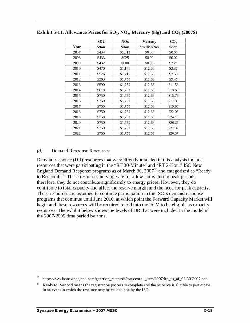
Synapse Energy Economics – 2007 AESC 5-19
Exhibit 5-11. Allowance Prices for SO2, NOx, Mercury (Hg) and CO2 (2007$)
SO2 NOx Mercury CO2 Year $/ton $/ton $million/ton $/ton 2007 $434 $1,013 $0.00 $0.00 2008 $433 $925 $0.00 $0.00 2009 $432 $800 $0.00 $2.21 2010 $470 $1,171 $12.66 $2.37 2011 $526 $1,715 $12.66 $2.53 2012 $563 $1,750 $12.66 $9.46 2013 $590 $1,750 $12.66 $11.56 2014 $610 $1,750 $12.66 $13.66 2015 $750 $1,750 $12.66 $15.76 2016 $750 $1,750 $12.66 $17.86 2017 $750 $1,750 $12.66 $19.96 2018 $750 $1,750 $12.66 $22.06 2019 $750 $1,750 $12.66 $24.16 2020 $750 $1,750 $12.66 $26.27 2021 $750 $1,750 $12.66 $27.32 2022 $750 $1,750 $12.66 $28.37
(d) Demand Response Resources
Demand response (DR) resources that were directly modeled in this analysis include resources that were participating in the “RT 30-Minute” and “RT 2-Hour” ISO New England Demand Response programs as of March 30, 200780 and categorized as “Ready to Respond.”81 These resources only operate for a few hours during peak periods; therefore, they do not contribute significantly to energy prices. However, they do contribute to total capacity and affect the reserve margin and the need for peak capacity. These resources are assumed to continue participation in the ISO’s demand response programs that continue until June 2010, at which point the Forward Capacity Market will begin and these resources will be required to bid into the FCM to be eligible as capacity resources. The exhibit below shows the levels of DR that were included in the model in the 2007-2009 time period by zone.
80 http://www.isonewengland.com/genrtion_resrcs/dr/stats/enroll_sum/2007/lrp_as_of_03-30-2007.ppt. 81 Ready to Respond means the registration process is complete and the resource is eligible to participate
in an event in which the resource may be called upon by the ISO.
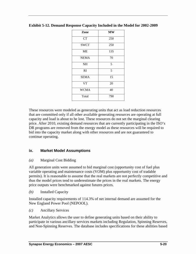
Synapse Energy Economics – 2007 AESC 5-20
Exhibit 5-12. Demand Response Capacity Included in the Model for 2002-2009
Zone MW
CT 250
SWCT 250
ME 135
NEMA 70
NH 5
RI 5
SEMA 15
VT 20
WCMA 40
Total 790
These resources were modeled as generating units that act as load reduction resources that are committed only if all other available generating resources are operating at full capacity and load is about to be lost. These resources do not set the marginal clearing price. After 2010, existing demand resources that are currently participating in the ISO’s DR programs are removed from the energy model as these resources will be required to bid into the capacity market along with other resources and are not guaranteed to continue operating.
ix. Market Model Assumptions
(a) Marginal Cost Bidding
All generation units were assumed to bid marginal cost (opportunity cost of fuel plus variable operating and maintenance costs (VOM) plus opportunity cost of tradable permits). It is reasonable to assume that the real markets are not perfectly competitive and thus the model prices tend to underestimate the prices in the real markets. The energy price outputs were benchmarked against futures prices.
(b) Installed Capacity
Installed capacity requirements of 114.3% of net internal demand are assumed for the New England Power Pool (NEPOOL).
(c) Ancillary Services
Market Analytics allows the user to define generating units based on their ability to participate in various ancillary services markets including Regulation, Spinning Reserves, and Non-Spinning Reserves. The database includes specifications for these abilities based
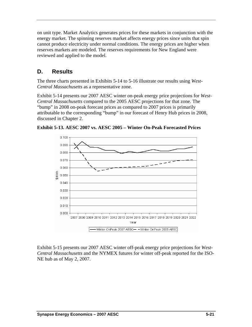
Synapse Energy Economics – 2007 AESC 5-21
on unit type. Market Analytics generates prices for these markets in conjunction with the energy market. The spinning reserves market affects energy prices since units that spin cannot produce electricity under normal conditions. The energy prices are higher when reserves markets are modeled. The reserves requirements for New England were reviewed and applied to the model.
D. Results The three charts presented in Exhibits 5-14 to 5-16 illustrate our results using West-Central Massachusetts as a representative zone.
Exhibit 5-14 presents our 2007 AESC winter on-peak energy price projections for West-Central Massachusetts compared to the 2005 AESC projections for that zone. The “bump” in 2008 on-peak forecast prices as compared to 2007 prices is primarily attributable to the corresponding “bump” in our forecast of Henry Hub prices in 2008, discussed in Chapter 2.
Exhibit 5-13. AESC 2007 vs. AESC 2005 – Winter On-Peak Forecasted Prices
Exhibit 5-15 presents our 2007 AESC winter off-peak energy price projections for West-Central Massachusetts and the NYMEX futures for winter off-peak reported for the ISO-NE hub as of May 2, 2007.
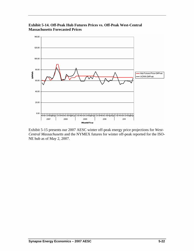
Synapse Energy Economics – 2007 AESC 5-22
Exhibit 5-14. Off-Peak Hub Futures Prices vs. Off-Peak West-Central Massachusetts Forecasted Prices
Exhibit 5-15 presents our 2007 AESC winter off-peak energy price projections for West-Central Massachusetts and the NYMEX futures for winter off-peak reported for the ISO-NE hub as of May 2, 2007.
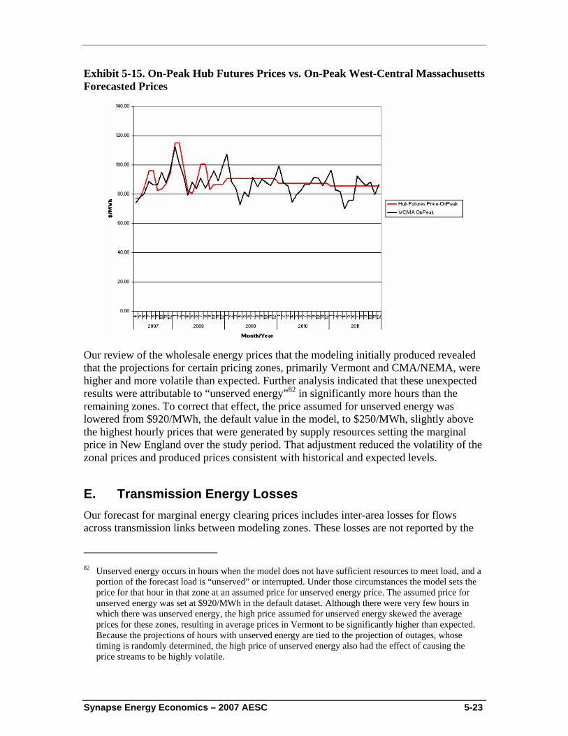
Synapse Energy Economics – 2007 AESC 5-23
Exhibit 5-15. On-Peak Hub Futures Prices vs. On-Peak West-Central Massachusetts Forecasted Prices
Our review of the wholesale energy prices that the modeling initially produced revealed that the projections for certain pricing zones, primarily Vermont and CMA/NEMA, were higher and more volatile than expected. Further analysis indicated that these unexpected results were attributable to “unserved energy”82 in significantly more hours than the remaining zones. To correct that effect, the price assumed for unserved energy was lowered from $920/MWh, the default value in the model, to $250/MWh, slightly above the highest hourly prices that were generated by supply resources setting the marginal price in New England over the study period. That adjustment reduced the volatility of the zonal prices and produced prices consistent with historical and expected levels.
E. Transmission Energy Losses Our forecast for marginal energy clearing prices includes inter-area losses for flows across transmission links between modeling zones. These losses are not reported by the
82 Unserved energy occurs in hours when the model does not have sufficient resources to meet load, and a
portion of the forecast load is “unserved” or interrupted. Under those circumstances the model sets the price for that hour in that zone at an assumed price for unserved energy price. The assumed price for unserved energy was set at $920/MWh in the default dataset. Although there were very few hours in which there was unserved energy, the high price assumed for unserved energy skewed the average prices for these zones, resulting in average prices in Vermont to be significantly higher than expected. Because the projections of hours with unserved energy are tied to the projection of outages, whose timing is randomly determined, the high price of unserved energy also had the effect of causing the price streams to be highly volatile.
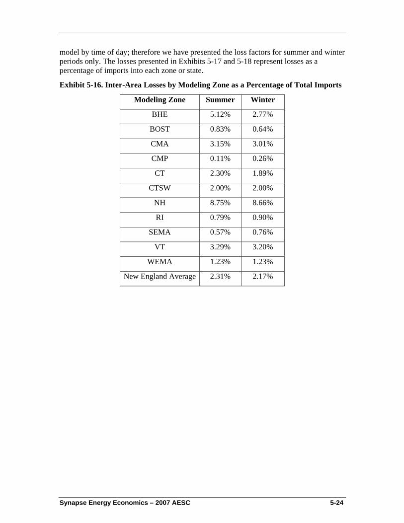
Synapse Energy Economics – 2007 AESC 5-24
model by time of day; therefore we have presented the loss factors for summer and winter periods only. The losses presented in Exhibits 5-17 and 5-18 represent losses as a percentage of imports into each zone or state.
Exhibit 5-16. Inter-Area Losses by Modeling Zone as a Percentage of Total Imports
Modeling Zone Summer Winter
BHE 5.12% 2.77%
BOST 0.83% 0.64%
CMA 3.15% 3.01%
CMP 0.11% 0.26%
CT 2.30% 1.89%
CTSW 2.00% 2.00%
NH 8.75% 8.66%
RI 0.79% 0.90%
SEMA 0.57% 0.76%
VT 3.29% 3.20%
WEMA 1.23% 1.23%
New England Average 2.31% 2.17%
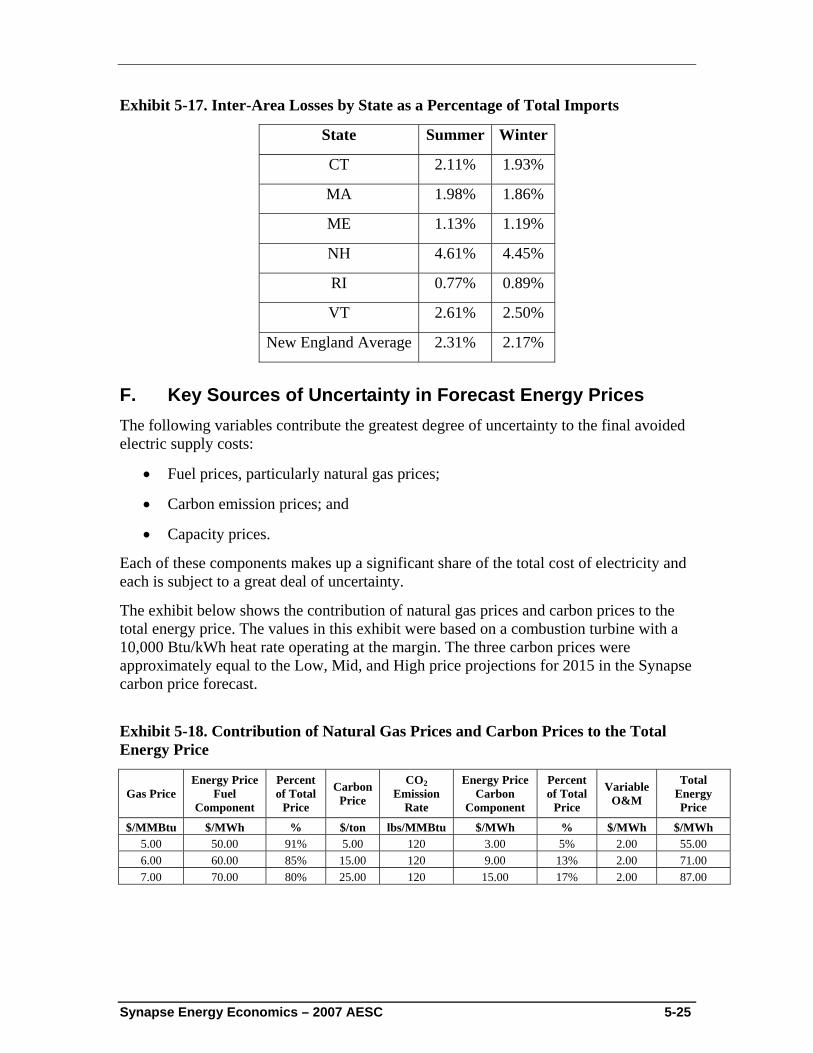
Synapse Energy Economics – 2007 AESC 5-25
Exhibit 5-17. Inter-Area Losses by State as a Percentage of Total Imports
State Summer Winter
CT 2.11% 1.93%
MA 1.98% 1.86%
ME 1.13% 1.19%
NH 4.61% 4.45%
RI 0.77% 0.89%
VT 2.61% 2.50%
New England Average 2.31% 2.17%
F. Key Sources of Uncertainty in Forecast Energy Prices The following variables contribute the greatest degree of uncertainty to the final avoided electric supply costs:
• Fuel prices, particularly natural gas prices;
• Carbon emission prices; and
• Capacity prices.
Each of these components makes up a significant share of the total cost of electricity and each is subject to a great deal of uncertainty.
The exhibit below shows the contribution of natural gas prices and carbon prices to the total energy price. The values in this exhibit were based on a combustion turbine with a 10,000 Btu/kWh heat rate operating at the margin. The three carbon prices were approximately equal to the Low, Mid, and High price projections for 2015 in the Synapse carbon price forecast. Exhibit 5-18. Contribution of Natural Gas Prices and Carbon Prices to the Total Energy Price
Gas Price Energy Price
Fuel Component
Percent of Total
Price
Carbon Price
CO2 Emission
Rate
Energy Price Carbon
Component
Percent of Total
Price
Variable O&M
Total Energy Price
$/MMBtu $/MWh % $/ton lbs/MMBtu $/MWh % $/MWh $/MWh 5.00 50.00 91% 5.00 120 3.00 5% 2.00 55.00 6.00 60.00 85% 15.00 120 9.00 13% 2.00 71.00 7.00 70.00 80% 25.00 120 15.00 17% 2.00 87.00
Synapse Energy Economics – 2007 AESC 5-26
Capacity prices are projected to add an estimated $10-14/MWh to the energy price.83 At a $71 energy price, the capacity prices make up 12-16% of the total electricity price. Carbon prices and capacity prices were based on projections of markets that are not yet operating, and therefore there is a great deal of speculation around these prices.
83 Connecticut Light and Power 2006 reconcilliation filing, March 30, 2007.
Synapse Energy Economics – 2007 AESC 6-1
6. Avoided Electricity Supply Costs This chapter provides a projection of avoided electricity costs and a description of the underlying assumptions.
Our avoided electricity supply costs were developed from projections of:
• Generally accepted components of avoided costs including
electric energy prices from section 5;
avoided costs from the Forward Capacity Market (FCM), adjusted for losses on the ISO-administered pool transmission facilities (PFT); and
avoided cost of compliance with RPS, and
• Additional components including
a retail adder, reflecting the risks and costs related to power procurement;
demand-reduction-induced price effects (DRIPE) for energy and capacity; and
environmental externalities.
These avoided electricity supply costs do not include several components of wholesale power costs that we consider to be largely or entirely unavoidable through DSM. These components include the locational forward reserve market, real-time operating reserves, automatic generation control (also called regulation), uplift, and the reliability contracts with particular generators.
As requested in the scope of work, avoided electricity supply costs are provided for the following geographic areas:
• Maine
• Vermont
• New Hampshire
• Connecticut (Statewide)
• Massachusetts (Statewide)
• Rhode Island
• SEMA (Southeast Massachusetts)
• WCMA (West-Central Massachusetts)
• NEMA (Northeast Massachusetts)
Synapse Energy Economics – 2007 AESC 6-2
• Rest of Massachusetts (Massachusetts excluding NEMA)
• Norwalk/Stamford
• Southwest Connecticut, including Norwalk/Stamford
• Southwest Connecticut, excluding Norwalk/Stamford
• Rest of Connecticut (Connecticut excluding all of Southwest Connecticut)
A. Avoided Cost of Compliance with RPS Our estimate of avoided costs includes the cost of avoiding additional costs under the RPS in the various states that have imposed such standards. In essence, these standards imply that the conventional power-supply mix imposes excessive costs and risks (which may be related to environmental damage, resource depletion, or price volatility), and that the costs of renewables are justified as mitigation. The amount of renewables required is tied to the amount of energy used, so this compliance cost is avoidable, just as the cost of environmental compliance on avoidable energy or new capacity is. Reduction in load due to DSM will reduce the RPS requirements of load serving entities (LSE) and therefore reduce the costs they seek to recover associated with complying with these requirements.
The RPS compliance costs that retail customers avoid through reductions in their energy usage is equal to the price of renewable energy in excess of market prices multiplied by the portion of retail load that a supplier must meet from renewable energy under the RPS. In other words,
Avoided RPS cost = renewable energy price premium * RPS percentage
So, in a year in which the renewable energy price premium was $50/MWh (or 5 cents/kWh) and the RPS percentage was 10%, the avoided RPS cost to a retail customer would be $0.50 cents/kWh.84
It was relatively easy to develop assumptions for RPS percentages by state over the study period, as they are generally specified in legislation or regulations. However, research found relatively few recent public projections of renewable energy price premiums in New England. One measure of that premium is the price at which Renewable Energy Credits (RECs) are trading and are projected to trade in the future. However, to develop an estimate of such a premium one needs to forecast prices in the wholesale energy market over the study period as well as to forecast prices in the market for “new renewables.” The difference between these two projections is an estimate of the prices at which RECs will trade.
Due to the absence of a definitive forecast, two methodologies were considered. The first is drawn from a recent study by researchers at the University of New Hampshire.85 The 84 5 cents/kWh * 10%. 85 Gittell, Ross and Magnusson, Matt; Economic Impact of a New Hampshire Renewable Portfolio
Standard, University of New Hampshire, February 2007.
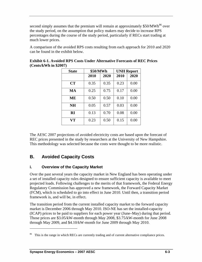
Synapse Energy Economics – 2007 AESC 6-3
second simply assumes that the premium will remain at approximately $50/MWh86 over the study period, on the assumption that policy makers may decide to increase RPS percentages during the course of the study period, particularly if RECs start trading at much lower prices.
A comparison of the avoided RPS costs resulting from each approach for 2010 and 2020 can be found in the exhibit below.
Exhibit 6-1. Avoided RPS Costs Under Alternative Forecasts of REC Prices (Cents/kWh in $2007)
State $50/MWh UNH Report 2010 2020 2010 2020
CT 0.35 0.35 0.23 0.00
MA 0.25 0.75 0.17 0.00
ME 0.50 0.50 0.10 0.00
NH 0.05 0.57 0.03 0.00
RI 0.13 0.70 0.08 0.00
VT 0.23 0.50 0.15 0.00
The AESC 2007 projections of avoided electricity costs are based upon the forecast of REC prices presented in the study by researchers at the University of New Hampshire. This methodology was selected because the costs were thought to be more realistic.
B. Avoided Capacity Costs
i. Overview of the Capacity Market
Over the past several years the capacity market in New England has been operating under a set of installed capacity rules designed to ensure sufficient capacity is available to meet projected loads. Following challenges to the merits of that framework, the Federal Energy Regulatory Commission has approved a new framework, the Forward Capacity Market (FCM), which is scheduled to go into effect in June 2010. Until then, a transition period framework is, and will be, in effect.
The transition period from the current installed capacity market to the forward capacity market is December 2006 through May 2010. ISO-NE has set the installed-capacity (ICAP) prices to be paid to suppliers for each power year (June–May) during that period. Those prices are $3.05/kW-month through May 2008, $3.75/kW-month for June 2008 through May 2009, and $4.10/kW-month for June 2009 through May 2010. 86 This is the range in which RECs are currently trading and of current alternative compliance prices.
Synapse Energy Economics – 2007 AESC 6-4
Under the FCM, ISO-NE will set the price for capacity each year based upon the results of an auction to be conducted three years in advance. However, the auction for the first FCM year, June 2010 through May 2011, will not be held until February 2008. Later in 2008 ISO-NE will conduct an auction for the second FCM year, June 2011 through May 2012. The basic structure for the auctions has been developed, but some important inputs – especially the amount of capacity that can be imported to each zone – have not been released.
The ISO will establish the FCM price from the auction results. For at least the first three FCM years (June 2010 through May 2013), the price for capacity will be constrained between a minimum and a maximum equal to -40% and +40% of a reference price respectively. The reference price for the first FCM year has been set at $90/kW-yr or $7.50/kW-month.
Suppliers will receive revenues equal to the quantity of capacity they provide times the auction price minus penalties for any failure to perform and minus an estimate of the energy profits (called peak energy rent, or PER) that would be earned by a generator with a 22,000 Btu/kWh.87 The PER that the hypothetical peaker would earn in each hour will be multiplied by the ratio of load in that hour to the peak load for the power year.
Load will pay costs equal to the quantity of capacity they are required to hold times the auction price, less credits for any supplier penalties and the PER. The quantity of capacity that a particular load is required to hold in each month is based on the contribution of that load to the ISO annual peak. As a result, the total cost of that capacity to that load, i.e., dollars per kW times required kW of capacity, is essentially fixed for an entire FCM year. The unit cost of capacity for a calendar year, $/kW-year, will be the average of five months at the cost for the power year ending in May of that calendar year and seven months for the power year starting in June.
ii. Transition Period Avoided Capacity Cost Forecast (2006 – May 2010)
Due to the fact that consumers must pay for all qualifying ICAP supply during the transition period, none of these capacity costs are avoidable. Public energy-efficiency programs that qualify for capacity payments under the transition period ICAP system will receive revenues that their program administrators can credit back to their retail customers in various ways.
iii. FCM Avoided Capacity Costs (June 2010 onwards)
According to current projections of peak capacity requirements, existing capacity and anticipated new additions, it is expected that New England will need some quantity of new capacity to come on-line in the summer of 2010 in order to maintain the desired reserve margin. Further additions will be required in subsequent years. In this section we describe our estimate of the annual value of potential new DSM programs in terms of avoiding the costs of those new capacity additions from June 2010 onward.
87 “Forward Capacity Market Payments, Performance and Charges,” ISO-NE, October 11, 2006, p. 9.
Synapse Energy Economics – 2007 AESC 6-5
The AESC 2007 estimate of avoided capacity costs under the FCM is neither designed, nor intended, to be a forecast of the annual price of capacity in the FCM. Instead, this is an estimate of the annual value of potential new DSM programs in terms of avoided capacity costs from June 2010 onward. The forecast was deliberately designed to estimate the cost of capacity in the FCM in the absence of any new DSM programs. This approach is consistent with the methodology that we used to estimate avoided electricity market prices. We understand that capacity prices in the first few years of the FCM will very likely be influenced by the quantity of demand reduction bid by new demand-response and energy-efficiency resources.
Our ability to develop this estimate was complicated by the absence of any empirical evidence or experience with this particular form of capacity auction, e.g., the bidding behavior of existing generators, new supply resources, and new efficiency resources. Thus, this forecast of avoided capacity costs under the FCM prices is inherently more uncertain than a forecast for a more-established market structure.
Given those caveats, our forecast of the unit cost of avoided capacity under the FCM is based on the assumptions listed below. Our approach is also discussed in the context of an illustrative example presented in Exhibit 6-3. Our assumptions are that:
• Most existing generation capacity will bid in as a “price-taker,” at or below the minimum FCM price;
• Some existing generation capacity will effectively88 submit bids somewhat above the minimum FCM price, reflecting their need for incremental capacity revenue to remain viable;
• there will be a substantial need for new capacity to satisfy RPS requirements, even after the bids received from existing generation and conventional new capacity;
• the incremental source of this new capacity will be new peakers;
• The FCM prices will be determined by the price of new peakers;
• The FCM prices will provide developers enough assurance to build enough peakers to meet the ISO-NE regional capability target, but no more; and
• Capacity will be added preferentially in the areas with the lowest reserves and the highest FCM prices, gradually equalizing reserves across the region. Connecticut and NEMA are most likely to have prices higher than average, and Maine is the zone most likely to have FCM prices below average.
The prices paid to generators should approximate the cost of new entry, which is assumed to be the fixed costs of a merchant combustion turbine, net of a conservative estimate of profits from energy sales.89
88 Existing generation owners do not submit regular bids but instead submit “de-list” bids.
Synapse Energy Economics – 2007 AESC 6-6
The three ISO adjustments to the FCM auction price were treated as follows:
(a) Non-Performance Penalties
Since bidders offering new capacity are likely to increase their bids to cover the expected level of outages and non-performance penalties, it was assumed that the price after non-performance penalties would be similar to the cost of new entry.
(b) Peak Energy Rent
The PER offset is likely to be very small.90 It was assumed that bidders will increase their bids to cover that small reduction.
(c) Reserve Margin
Each kW of load on the ISO system will be required to support more than a kW of supply. A reserve margin of 14.3% was assumed, plus an allowance for the demand-response resources that were assumed in the determination of the required reserves.
89 New peakers are also likely to receive some revenues in the forward reserve market (although this
would require foregoing some energy revenues) and the real-time reserve market. Since the ISO will reduce the forward reserve price by the forward capacity price, and since the forward capacity auction will be run long before the forward reserve auction, we assume that developers will not reduce their capacity bids based on potential future reserve payments.
90 Over the period from 2005 to the present, the PER would have been less than $1/kW-year.
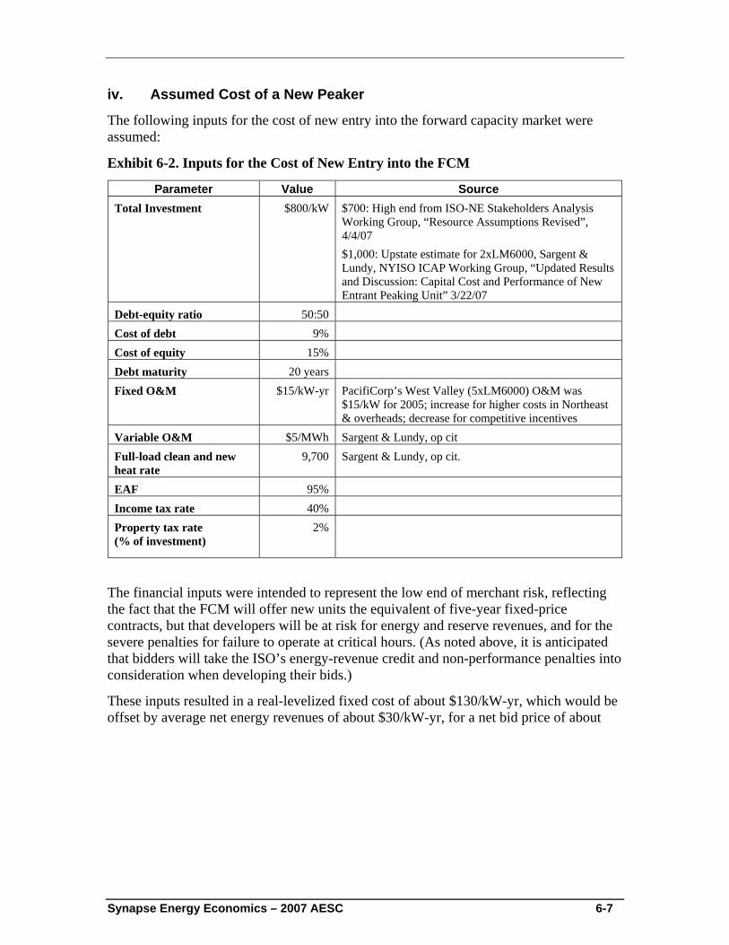
Synapse Energy Economics – 2007 AESC 6-7
iv. Assumed Cost of a New Peaker
The following inputs for the cost of new entry into the forward capacity market were assumed:
Exhibit 6-2. Inputs for the Cost of New Entry into the FCM
Parameter Value Source Total Investment $800/kW $700: High end from ISO-NE Stakeholders Analysis
Working Group, “Resource Assumptions Revised”, 4/4/07 $1,000: Upstate estimate for 2xLM6000, Sargent & Lundy, NYISO ICAP Working Group, “Updated Results and Discussion: Capital Cost and Performance of New Entrant Peaking Unit” 3/22/07
Debt-equity ratio 50:50 Cost of debt 9% Cost of equity 15% Debt maturity 20 years Fixed O&M $15/kW-yr PacifiCorp’s West Valley (5xLM6000) O&M was
$15/kW for 2005; increase for higher costs in Northeast & overheads; decrease for competitive incentives
Variable O&M $5/MWh Sargent & Lundy, op cit Full-load clean and new heat rate
9,700 Sargent & Lundy, op cit.
EAF 95% Income tax rate 40% Property tax rate (% of investment)
2%
The financial inputs were intended to represent the low end of merchant risk, reflecting the fact that the FCM will offer new units the equivalent of five-year fixed-price contracts, but that developers will be at risk for energy and reserve revenues, and for the severe penalties for failure to operate at critical hours. (As noted above, it is anticipated that bidders will take the ISO’s energy-revenue credit and non-performance penalties into consideration when developing their bids.)
These inputs resulted in a real-levelized fixed cost of about $130/kW-yr, which would be offset by average net energy revenues of about $30/kW-yr, for a net bid price of about
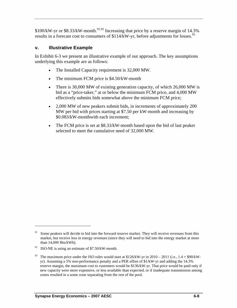
Synapse Energy Economics – 2007 AESC 6-8
$100/kW-yr or $8.33/kW-month.91,92 Increasing that price by a reserve margin of 14.3% results in a forecast cost to consumers of $114/kW-yr, before adjustments for losses.93
v. Illustrative Example
In Exhibit 6-3 we present an illustrative example of our approach. The key assumptions underlying this example are as follows:
• The Installed Capacity requirement is 32,000 MW.
• The minimum FCM price is $4.50/kW-month
• There is 30,000 MW of existing generation capacity, of which 26,000 MW is bid as a “price-taker,” at or below the minimum FCM price, and 4,000 MW effectively submits bids somewhat above the minimum FCM price;
• 2,000 MW of new peakers submit bids, in increments of approximately 200 MW per bid with prices starting at $7.50 per kW-month and increasing by $0.083/kW-monthwith each increment;
• The FCM price is set at $8.33/kW-month based upon the bid of last peaker selected to meet the cumulative need of 32,000 MW.
91 Some peakers will decide to bid into the forward reserve market. They will receive revenues from this
market, but receive less in energy revenues (since they will need to bid into the energy market at more than 14,000 Btu/kWh).
92 ISO-NE is using an estimate of $7.50/kW-month.
93 The maximum price under the ISO rules would start at $126/kW-yr in 2010 – 2011 (i.e., 1.4 × $90/kW-yr). Assuming a 5% non-performance penalty and a PER offset of $1/kW-yr and adding the 14.3% reserve margin, the maximum cost to customers would be $136/kW-yr. That price would be paid only if new capacity were more expensive, or less available than expected, or if inadequate transmission among zones resulted in a some zone separating from the rest of the pool.
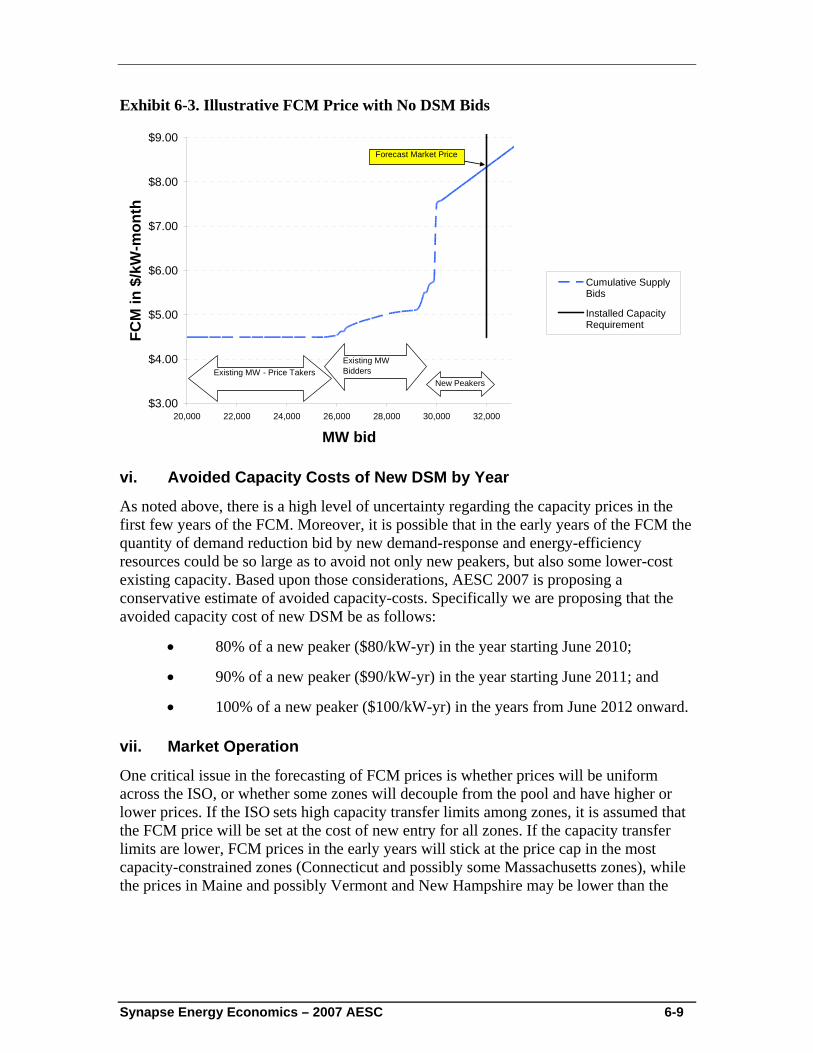
Synapse Energy Economics – 2007 AESC 6-9
Exhibit 6-3. Illustrative FCM Price with No DSM Bids
$3.00
$4.00
$5.00
$6.00
$7.00
$8.00
$9.00
20,000 22,000 24,000 26,000 28,000 30,000 32,000
MW bid
FCM
in $
/kW
-mon
th
Cumulative SupplyBids
Installed CapacityRequirement
Forecast Market Price
Existing MW - Price TakersNew Peakers
Existing MW Bidders
vi. Avoided Capacity Costs of New DSM by Year
As noted above, there is a high level of uncertainty regarding the capacity prices in the first few years of the FCM. Moreover, it is possible that in the early years of the FCM the quantity of demand reduction bid by new demand-response and energy-efficiency resources could be so large as to avoid not only new peakers, but also some lower-cost existing capacity. Based upon those considerations, AESC 2007 is proposing a conservative estimate of avoided capacity-costs. Specifically we are proposing that the avoided capacity cost of new DSM be as follows:
• 80% of a new peaker ($80/kW-yr) in the year starting June 2010;
• 90% of a new peaker ($90/kW-yr) in the year starting June 2011; and
• 100% of a new peaker ($100/kW-yr) in the years from June 2012 onward.
vii. Market Operation
One critical issue in the forecasting of FCM prices is whether prices will be uniform across the ISO, or whether some zones will decouple from the pool and have higher or lower prices. If the ISO sets high capacity transfer limits among zones, it is assumed that the FCM price will be set at the cost of new entry for all zones. If the capacity transfer limits are lower, FCM prices in the early years will stick at the price cap in the most capacity-constrained zones (Connecticut and possibly some Massachusetts zones), while the prices in Maine and possibly Vermont and New Hampshire may be lower than the
Synapse Energy Economics – 2007 AESC 6-10
cost of new entry.94 In the absence of any experience with this market, estimating the lower prices is a matter of judgment. Over time, concentration of new resources in the higher-priced zones would tend to eliminate the FCM price differentials among zones.
The ISO committed to finalize the topology (which would include the local sourcing requirements and transfer limits) for the first forward-capacity auction in December 2006 and post the final assumptions early in January 2007.95 The assumptions used in AESC 2007 are consistent with those posted by the ISO in mid-July 2007. If the capacity transfer limits are the same as the estimates the ISO sponsored in the testimony of David LaPlante in the Locational ICAP Filing,96 there will be no locational zones in the FCM.97
Our forecast of the avoided cost of capacity in the FCM is $100/kW-yr in 2007 dollars, based on the cost of new peakers, from June 2010 through the end of the study period.
viii. Reliability-Must-Run (RMR) Contracts
Our study does not include any avoidable costs for reliability contracts for the reasons outlined herein.
The FCM price projected in this study covers the entire revenue requirement of four of the ten plants described in Exhibit 5-8, so those plants should not require reliability agreements.98 The combined-cycle plants are likely to earn at least $80/kW-yr of profit in the energy markets, so Berkshire, Milford and Bridgeport Energy should be economic without any special treatment. With the market energy prices projected in this project, and some uplift compensation for cycling, New Haven Harbor should receive more than its revenue requirement or at the very least roughly break even. In addition, the cost of keeping this unit on line is likely to be less than the revenue requirements which the ISO agreed to pay them. That leaves only the West Springfield CTs and Bridgeport Harbor 2 at risk. The FCM should be sufficient to encourage some developer to build new capacity in WCMA, if Con Edison bids West Springfield into the forward capacity auction at a price close to the $161/kW-year revenue requirement. Bridgeport Harbor 2 may no longer be needed after the operation of the Southwest Connecticut transmission upgrade and other changes in the system. At worst, the cost of the remaining reliability contract would be under $5 million for Bridgeport Harbor 2 ($46/kW-year × 130 MW). It is not clear what magnitude of load reductions would avoid the need for Bridgeport Harbor 2. 94 The caps are 1.4 × $90/kW-yr, or $126/kW-yr in 2010 – 2011; 1.4 times the average of $90 and the
first-year price ($126) or $151/kW-yr in 2011 – 2012; and 1.4 × (.25 × $90 + .75 × ($126 + $151) ÷ 2) = $177/kW-yr in 2012–2013.
95 “Establishing New England System Topology Assumptions for the Forward Capacity Market,” Transmission Owners Meeting, October 19, 2006, p. 4.
96 FERC Docket No. ER03-563-030, August 31, 2004. 97 This is also the conclusion of “Report on the Electricity Sector Needs of Connecticut, 2007 – 2021,”
London Economics International, on behalf of the Connecticut DPUC, August 25, 2006. 98 As noted above, DSM resources may reduce actual FCM prices in the first few years of the market’s
operation. If those conditions materialize, some of the RMR generators may request new contracts, creating the opportunity for additional DSM to avoid RMR costs. This factor would tend to offset the reduction in avoidable FCM prices and stabilize the value of DSM.
Synapse Energy Economics – 2007 AESC 6-11
ix. Comparison to 2005 AESC Estimates of Capacity Costs
The 2005 AESC study, based on the administrative “demand-curve” method then proposed by ISO-NE for setting locational installed capacity prices, estimated capacity prices that varied by year and zone. The levelized capacity prices for 2006–2020 (in 2005 dollars, excluding reserves) were $48/kW-year for Maine, $71/kW-year–$74/kW-year in various parts of Connecticut, $72/kW-year for Boston, and $68/kW-year in other zones. Even with reserves and inflation, the values from the 2005 study are lower than the current estimates, primarily due to the differences in the anticipated ISO capacity markets.
x. Derivation of FCM Load Reduction Credits
When preparing our analysis of the FCM, we estimated the capacity credits that program administrators programs would receive if they bid DSM programs into the forward capacity auction. Those estimated capacity credits are presented in our Avoided Electricity Costs in Appendix E. These revenues reflect our estimates of the approximate levels at which prices will clear in the FCM. Those levels are:
• $60/kW-yr in the year starting June 2010;
• 80/kW-yr in the year starting June 2011; and
• 100/kW-yr in the years from June 2012 onward.
It is important to note that these capacity credit revenues are not a component of the AESC 2007 avoided electricity costs.99 Instead, we have simply provided this estimate for the convenience of program administrators. For example, regulators may ask program administrators for an estimate of the FCM revenues they expect from the programs they bid into that market.
Our estimation of those credits is based upon our projection of the prices in the FCM and the procedure that ISO-NE will follow to determine credits for load reduction resources from those prices.100 Under that procedure ISO-NE will determine the credit, i.e., $/kW x kW of load reduction, to provide a load reduction resource based upon its actual performance in two key periods, a summer period of June, July, and August, and a winter period of December and January. In the remaining months the ISO will pay a capacity credit to that resource based on its performance in each of those periods, specifically:
• In April, May, September, October, and November, the ISO will pay a credit equal to the resource’s average reduction in June, July, and August; and
99 These revenues are not benefits for New England customers as a whole under the Total Resource Cost
(TRC) cost-benefit test, since customers will be paying the FCM charges, as well as getting the benefits of the FCM revenues offsetting DSM costs.
100 For more detail and the treatment of dispatchable demand-side resources, see “Introduction to Demand Resource Participation in New England’s Forward Capacity Market,” ISO-NE presentation at the Sheraton Springfield Monarch Place Hotel, February 16, 2007.
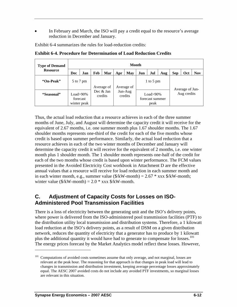
Synapse Energy Economics – 2007 AESC 6-12
• In February and March, the ISO will pay a credit equal to the resource’s average reduction in December and January.
Exhibit 6-4 summarizes the rules for load-reduction credits:
Exhibit 6-4. Procedure for Determination of Load Reduction Credits
Month Type of Demand Resource
Dec Jan Feb Mar Apr May Jun Jul Aug Sep Oct Nov
“On-Peak”
5 to 7 pm
1 to 5 pm
“Seasonal”
Load>90% forecast
winter peak
Average of Dec & Jan
credits
Average of Jun-Aug credits Load>90%
forecast summer peak
Average of Jun-Aug credits
Thus, the actual load reduction that a resource achieves in each of the three summer months of June, July, and August will determine the capacity credit it will receive for the equivalent of 2.67 months, i.e. one summer month plus 1.67 shoulder months. The 1.67 shoulder months represents one-third of the credit for each of the five months whose credit is based upon summer performance. Similarly, the actual load reduction that a resource achieves in each of the two winter months of December and January will determine the capacity credit it will receive for the equivalent of 2 months, i.e. one winter month plus 1 shoulder month. The 1 shoulder month represents one-half of the credit for each of the two months whose credit is based upon winter performance. The FCM values presented in the Avoided Electricity Cost workbook in Attachment D are the effective annual values that a resource will receive for load reduction in each summer month and in each winter month, e.g., summer value ($/kW-month) = 2.67 * xxx $/kW-month; winter value ($/kW-month) = 2.0 * xxx $/kW-month.
C. Adjustment of Capacity Costs for Losses on ISO-Administered Pool Transmission Facilities There is a loss of electricity between the generating unit and the ISO’s delivery points, where power is delivered from the ISO-administered pool transmission facilities (PTF) to the distribution utility local transmission and distribution systems. Therefore, a 1 kilowatt load reduction at the ISO’s delivery points, as a result of DSM on a given distribution network, reduces the quantity of electricity that a generator has to produce by 1 kilowatt plus the additional quantity it would have had to generate to compensate for losses.101 The energy prices forecast by the Market Analytics model reflect these losses. However, 101 Computations of avoided costs sometimes assume that only average, and not marginal, losses are
relevant at the peak hour. The reasoning for that approach is that changes in peak load will lead to changes in transmission and distribution investment, keeping average percentage losses approximately equal. The AESC 2007 avoided costs do not include any avoided PTF investments, so marginal losses are relevant in this situation.
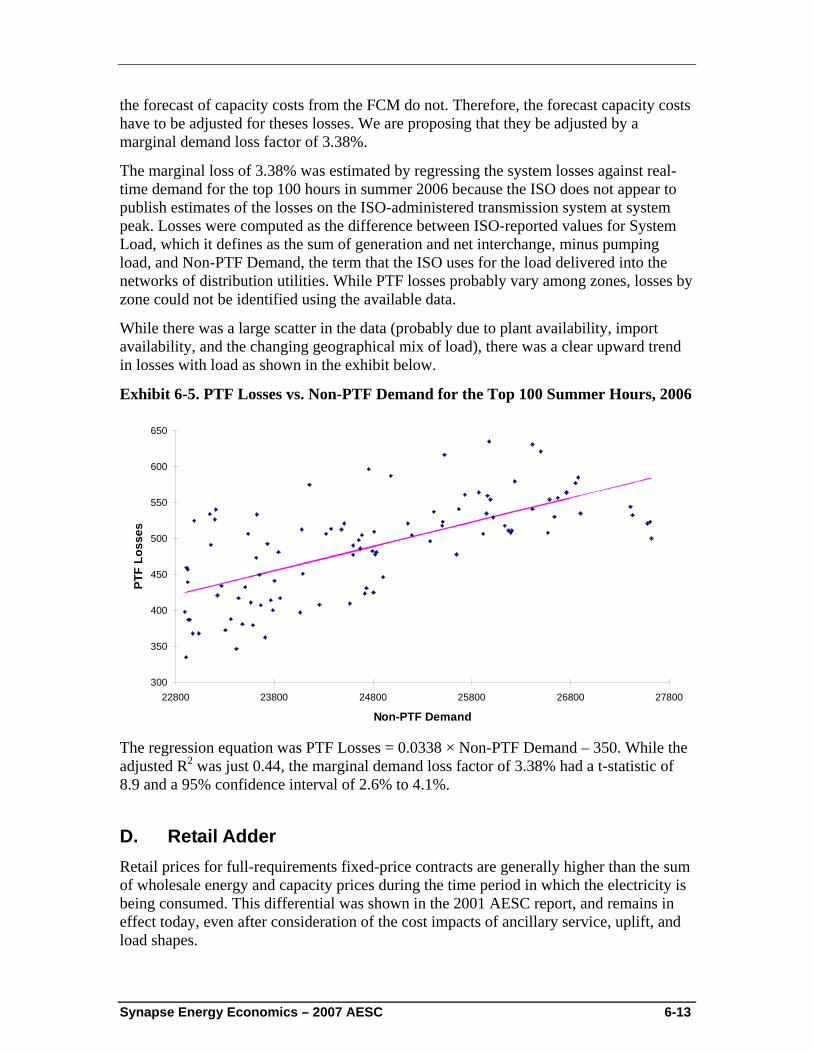
Synapse Energy Economics – 2007 AESC 6-13
the forecast of capacity costs from the FCM do not. Therefore, the forecast capacity costs have to be adjusted for theses losses. We are proposing that they be adjusted by a marginal demand loss factor of 3.38%.
The marginal loss of 3.38% was estimated by regressing the system losses against real-time demand for the top 100 hours in summer 2006 because the ISO does not appear to publish estimates of the losses on the ISO-administered transmission system at system peak. Losses were computed as the difference between ISO-reported values for System Load, which it defines as the sum of generation and net interchange, minus pumping load, and Non-PTF Demand, the term that the ISO uses for the load delivered into the networks of distribution utilities. While PTF losses probably vary among zones, losses by zone could not be identified using the available data.
While there was a large scatter in the data (probably due to plant availability, import availability, and the changing geographical mix of load), there was a clear upward trend in losses with load as shown in the exhibit below.
Exhibit 6-5. PTF Losses vs. Non-PTF Demand for the Top 100 Summer Hours, 2006
300
350
400
450
500
550
600
650
22800 23800 24800 25800 26800 27800
Non-PTF Demand
PTF
Loss
es
The regression equation was PTF Losses = 0.0338 × Non-PTF Demand – 350. While the adjusted R2 was just 0.44, the marginal demand loss factor of 3.38% had a t-statistic of 8.9 and a 95% confidence interval of 2.6% to 4.1%.
D. Retail Adder Retail prices for full-requirements fixed-price contracts are generally higher than the sum of wholesale energy and capacity prices during the time period in which the electricity is being consumed. This differential was shown in the 2001 AESC report, and remains in effect today, even after consideration of the cost impacts of ancillary service, uplift, and load shapes.
Synapse Energy Economics – 2007 AESC 6-14
The primary factor underlying the retail adder appears to be costs suppliers incur to mitigate their risk of under-recovering their costs. These risks arise from the potential for their supply costs to exceed their revenues, i.e., under contracts in which suppliers do not have a “true-up” provision or adjustment to ensure that their revenues equal their costs. The potential for supply costs to exceed revenues arises due to factors such as unexpected variations in weather, economic activity and and/or customer migration. For example, during hot summers and cold winters LSEs may need to procure additional energy at shortage prices while in mild weather they may have excess supply under contract that they need to “dump” into the wholesale market at a loss. The same pattern holds in economic boom and bust cycles. In addition, the suppliers of power for utility standard-service offers run risks related to migration of customer load from utility service to competitive supply (presumably at times of low market prices, leaving the supplier to sell surplus into a weak market at a loss) and from competitive supply to the utility service (at times of high market prices, forcing the supplier to purchase additional power in a high-cost market). No utility sponsor of this project was able to provide public information on the retail adders implicit in the prices bid by their suppliers. Analyses of confidential supplier bids in other projects suggests that a 10% retail adder is realistic.102 This adder was applied to the avoided wholesale energy prices and avoided wholesale capacity prices.103 The details of the risks and costs of serving load are somewhat different in Vermont and for Public Service of New Hampshire, where vertically-integrated utilities procure power from owned resources and a variety of long- and short-term contracts. It is possible that those utilities face risks similar in nature and magnitude to those of the competitive suppliers for new, marginal supplies. However, we were unable to confirm the nature and magnitude of the risks, and associated costs of risk mitigation, that those utilities face.
E. Demand-Reduction-Induced Price Effects (DRIPE) for Energy and Capacity The Demand-Reduction-Induced Price Effect (DRIPE) is the reduction in prices in the wholesale energy and capacity markets resulting from the reduction in need for energy and/or capacity due to efficiency and/or demand response programs. This section describes the AESC 2007 estimates of energy DRIPE and capacity DRIPE. Our estimates indicate that the DRIPE effects are very small when expressed in terms of an impact on market prices, i.e., reductions of a fraction of a percent. Moreover, we project that those effects will dissipate over four to five years as the market reacts to the new, lower level of energy and capacity required. However, the DRIPE impacts are significant when 102 The magnitude of the adder is smaller for near-term procurements than for power procured years in
advance, and is higher for congestion into load pockets (such as Connecticut) than for supply to unconstrained areas. The 10% value is a reasonable estimate for the standard-service procurement schedules in most states.
103 We are unsure how suppliers will structure power supply contracts to capture the risk premium for energy and capacity moving forward. As a result, our recommendation is that the retail adder be applied uniformly to both energy and capacity values.
Synapse Energy Economics – 2007 AESC 6-15
expressed in absolute dollar terms. Very small impacts on market prices, when applied to all energy and capacity being purchased in the market, translate into large absolute dollar amounts.
i. Energy DRIPE
Energy-efficiency measures installed in any one year will have an immediate downward effect on energy prices because the lower load growth will allow lower-cost resources to be at the margin—and set the price—in more hours. This impact is referred to as energy DRIPE. However, those price effects are not likely to persist many years, despite the persistence of energy savings. The lower energy prices will tend to change the mix of generation used to supply the market, which in turn will eventually lead to higher prices erasing the effects of lower loads.
DRIPE in the energy market was estimated based on the following three factors:
• The effect of load reduction on market energy prices, if all energy traded in the spot market and the supply system did not change as a result of DRIPE effects;
• The pace at which supply will adapt to energy-efficiency load reductions; and
• The percentage of power supply to retail customers that is subject to market prices in the current year and each future year.
The final DRIPE was the product of the direct effect from the first factor, times the percent of the effect not yet eliminated by supply adaptation from the second factor, times the percentage of power supply that is subject to market prices from the third factor. The DRIPE value may differ by month (or season) and zone.
(a) Effect of Load Reduction on Market Energy Prices
The determination of DRIPE starts with an analysis of the historical variation in locational energy market prices as a function of variation in zonal and regional loads. To minimize the effect of changes in fuel prices, each month was analyzed separately, over a period of at least the last year. Due to the unusual weather in the winter of 2006–2007, analyses from the preceding winter were included.
The basic form of this historical analysis was a regression of day-ahead hourly zonal price in dollars per MWh against both day-ahead load in the zone and day-ahead load in the rest of the ISO control area (rest of pool, or ROP). If one of the resulting coefficients was implausible or insignificant, the zonal price was regressed on total pool load and the resulting coefficient was used for both the own-zone and ROP load. These analyses were performed separately for on- and off-peak hours, since it was expected (and observed) that the slope of market price as a function of load would be higher on-peak.
These results indicate that each additional MW of load in a zone typically increases price in that zone by from 0.4¢/MWh to 4.5¢/MWh, depending on the zone and month. An additional MW of load in the ROP typically increases prices from 0.3¢/MWh to 2.0¢/MWh. The price effect is consistently higher on-peak than off-peak.
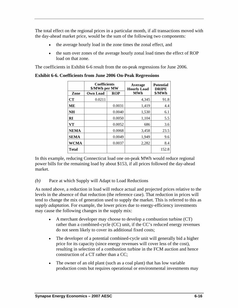
Synapse Energy Economics – 2007 AESC 6-16
The total effect on the regional prices in a particular month, if all transactions moved with the day-ahead market price, would be the sum of the following two components:
• the average hourly load in the zone times the zonal effect, and
• the sum over zones of the average hourly zonal load times the effect of ROP load on that zone.
The coefficients in Exhibit 6-6 result from the on-peak regressions for June 2006.
Exhibit 6-6. Coefficients from June 2006 On-Peak Regressions
Coefficients $/MWh per MW
Zone Own Load ROP
Average Hourly Load
MWh
Potential DRIPE $/MWh
CT 0.0211 4,345 91.8 ME 0.0031 1,419 4.4 NH 0.0040 1,530 6.1 RI 0.0050 1,104 5.5 VT 0.0052 686 3.6 NEMA 0.0068 3,458 23.5 SEMA 0.0049 1,949 9.6 WCMA 0.0037 2,282 8.4 Total 152.8
In this example, reducing Connecticut load one on-peak MWh would reduce regional power bills for the remaining load by about $153, if all prices followed the day-ahead market.
(b) Pace at which Supply will Adapt to Load Reductions
As noted above, a reduction in load will reduce actual and projected prices relative to the levels in the absence of that reduction (the reference case). That reduction in prices will tend to change the mix of generation used to supply the market. This is referred to this as supply adaptation. For example, the lower prices due to energy-efficiency investments may cause the following changes in the supply mix:
• A merchant developer may choose to develop a combustion turbine (CT) rather than a combined-cycle (CC) unit, if the CC’s reduced energy revenues do not seem likely to cover its additional fixed costs;
• The developer of a potential combined-cycle unit will generally bid a higher price for its capacity (since energy revenues will cover less of the cost), resulting in selection of a combustion turbine in the FCM auction and hence construction of a CT rather than a CC;
• The owner of an old plant (such as a coal plant) that has low variable production costs but requires operational or environmental investments may
Synapse Energy Economics – 2007 AESC 6-17
decide to retire or mothball the plant, due to the lower energy revenues from continued operation;104 and/or
• The owner of a baseload or intermediate plant may decide to defer spending that would increase its capacity or reliability, since the incremental revenues would not justify the expenditures.
As the supply mix changes in these and similar ways, energy prices would tend to increase back towards reference case levels. Once this supply adaptation has caused energy prices to recover from the effects of the load reduction, the future decisions by developers, owners and the ISO should be essentially the same as they would have been without the load reduction. Thus, supply adaptation ceases once the price effect has been extinguished.
Supply adaptation will take several years to eliminate all DRIPE, since the supply system cannot immediately respond to the reduction in load. For example, the downward pressure on energy prices due to efficiency measures implemented in one year (e.g., 2009) may not immediately affect expectations of market energy prices. The reductions may only be reflected in decisions to bid FCM capacity in the next year (e.g., 2010) for capacity to be delivered three years later (e.g., 2013).
Estimating the extent of delay in adaptation of the energy market to efficiency-related load reductions is subject to considerable uncertainty. Considering project lead time (including the operation of the FCM market) and past experience with over- and under-building cycles, it is believed that supply adaptation will offset the price effect of DSM over a period of four years after the installation of the measure, with an offset of 0% in years one and two, 35% in year three and 65% in year four.
(c) Share of Retail Power Supply at Current Market Prices
Were all retail power supply provided under cost-of-service pricing or long-term contracts, a short-term reduction in wholesale market prices would have little effect on retail supply prices paid by customers. At the other extreme, if retail customers were being supplied 100% from the spot market and paying spot-market prices, they would experience the benefits of short-term reductions in wholesale market prices fully and immediately. The actual mix of power supply under contract for various periods into the future varies among the states, among the utilities within some states, between municipal utilities and independently owned utilities (IOUs), and between customers on standard utility offer (standard service, default service, last-resort service, etc.) and those served by competitive suppliers. The standard-offer mixes are subject to legislative and/or regulatory change.
The exhibit below summarizes the contracting patterns for power supply by state and type of utility and/or supply arrangement.
104 This is not an entirely hypothetical concern, given the costs of upgrading existing coal (and some oil)
plants to meet tighter limits on air emissions and (for Brayton Point) use of cooling water.
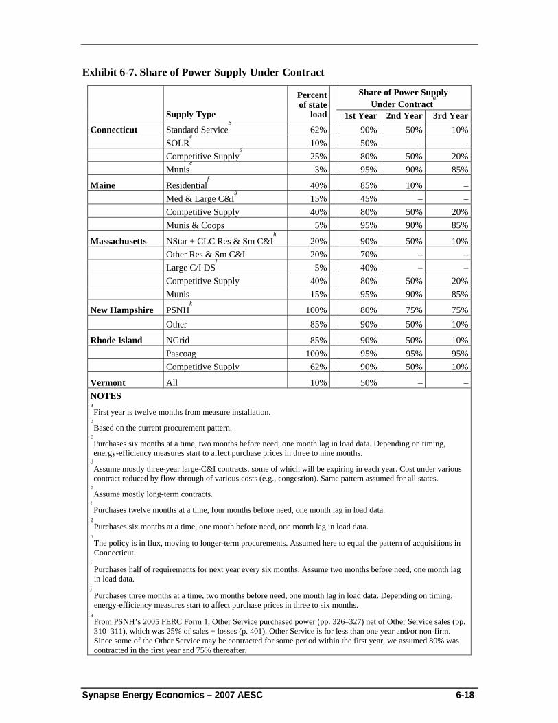
Synapse Energy Economics – 2007 AESC 6-18
Exhibit 6-7. Share of Power Supply Under Contract
Share of Power Supply Under Contract
a
Supply Type
Percent of state
load 1st Year 2nd Year 3rd YearConnecticut Standard Service
b 62% 90% 50% 10%
SOLRc 10% 50% – –
Competitive Supplyd 25% 80% 50% 20%
Munise 3% 95% 90% 85%
Maine Residentialf 40% 85% 10% –
Med & Large C&Ig 15% 45% – –
Competitive Supply 40% 80% 50% 20% Munis & Coops 5% 95% 90% 85%
Massachusetts NStar + CLC Res & Sm C&Ih 20% 90% 50% 10%
Other Res & Sm C&Ii 20% 70% – –
Large C/I DSj 5% 40% – –
Competitive Supply 40% 80% 50% 20% Munis 15% 95% 90% 85%
New Hampshire PSNHk 100% 80% 75% 75%
Other 85% 90% 50% 10%
Rhode Island NGrid 85% 90% 50% 10% Pascoag 100% 95% 95% 95% Competitive Supply 62% 90% 50% 10%
Vermont All 10% 50% – –NOTES a First year is twelve months from measure installation.
b Based on the current procurement pattern.
c Purchases six months at a time, two months before need, one month lag in load data. Depending on timing, energy-efficiency measures start to affect purchase prices in three to nine months.
d Assume mostly three-year large-C&I contracts, some of which will be expiring in each year. Cost under various contract reduced by flow-through of various costs (e.g., congestion). Same pattern assumed for all states.
e Assume mostly long-term contracts.
f Purchases twelve months at a time, four months before need, one month lag in load data.
g Purchases six months at a time, one month before need, one month lag in load data.
h The policy is in flux, moving to longer-term procurements. Assumed here to equal the pattern of acquisitions in Connecticut.
i Purchases half of requirements for next year every six months. Assume two months before need, one month lag in load data.
j Purchases three months at a time, two months before need, one month lag in load data. Depending on timing, energy-efficiency measures start to affect purchase prices in three to six months.
k From PSNH’s 2005 FERC Form 1, Other Service purchased power (pp. 326–327) net of Other Service sales (pp. 310–311), which was 25% of sales + losses (p. 401). Other Service is for less than one year and/or non-firm. Since some of the Other Service may be contracted for some period within the first year, we assumed 80% was contracted in the first year and 75% thereafter.
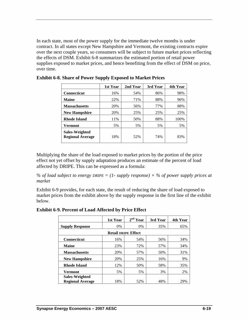
Synapse Energy Economics – 2007 AESC 6-19
In each state, most of the power supply for the immediate twelve months is under contract. In all states except New Hampshire and Vermont, the existing contracts expire over the next couple years, so consumers will be subject to future market prices reflecting the effects of DSM. Exhibit 6-8 summarizes the estimated portion of retail power supplies exposed to market prices, and hence benefiting from the effect of DSM on price, over time.
Exhibit 6-8. Share of Power Supply Exposed to Market Prices
1st Year 2nd Year 3rd Year 4th Year Connecticut 16% 54% 86% 98% Maine 22% 71% 88% 96% Massachusetts 20% 56% 77% 88% New Hampshire 20% 25% 25% 25% Rhode Island 11% 50% 88% 100% Vermont 5% 5% 5% 5% Sales-Weighted Regional Average 18% 52% 74% 83%
Multiplying the share of the load exposed to market prices by the portion of the price effect not yet offset by supply adaptation produces an estimate of the percent of load affected by DRIPE. This can be expressed as a formula:
% of load subject to energy DRIPE = (1- supply response) × % of power supply prices at market
Exhibit 6-9 provides, for each state, the result of reducing the share of load exposed to market prices from the exhibit above by the supply response in the first line of the exhibit below.
Exhibit 6-9. Percent of Load Affected by Price Effect
1st Year 2nd Year 3rd Year 4th Year Supply Response 0% 0% 35% 65%
Retail DRIPE Effect Connecticut 16% 54% 56% 34% Maine 23% 72% 57% 34% Massachusetts 20% 57% 50% 31% New Hampshire 20% 25% 16% 9% Rhode Island 12% 50% 58% 35% Vermont 5% 5% 3% 2% Sales-Weighted Regional Average 18% 52% 48% 29%
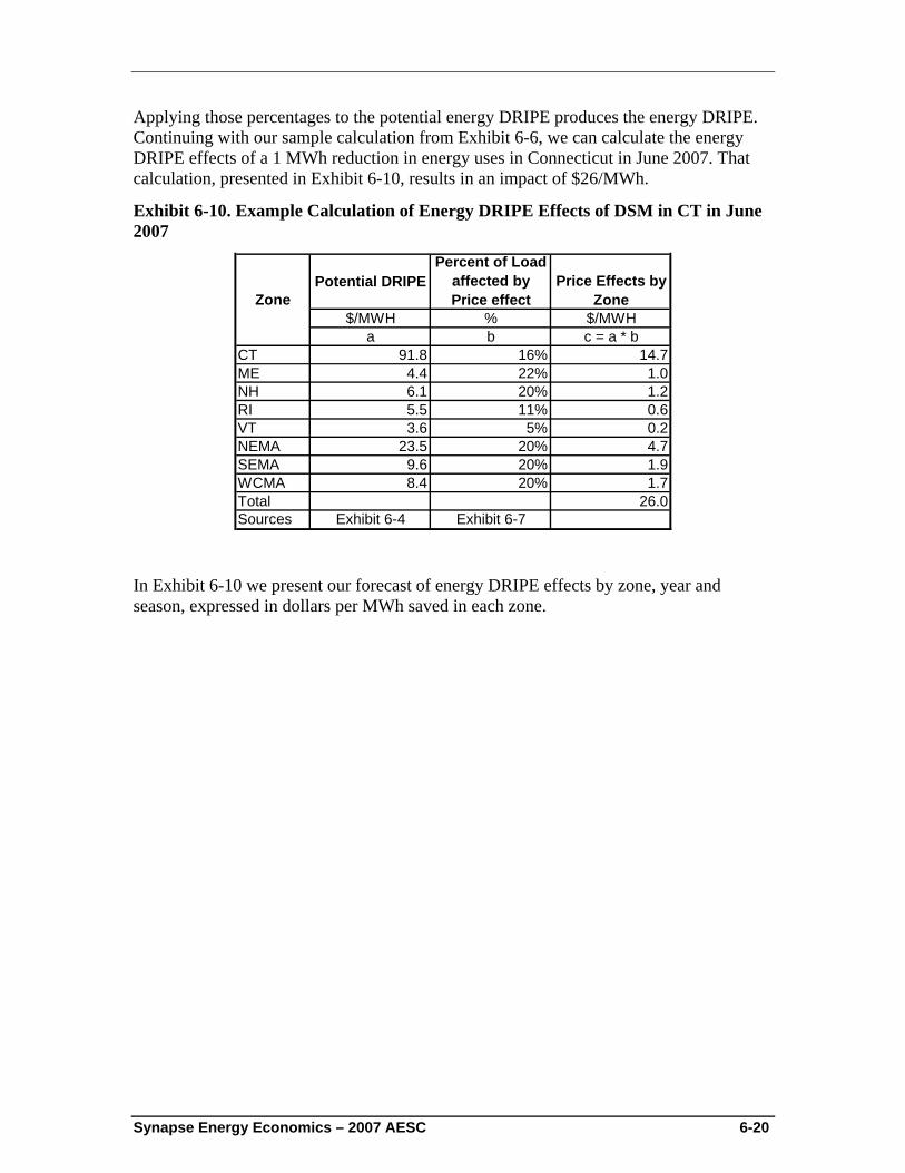
Synapse Energy Economics – 2007 AESC 6-20
Applying those percentages to the potential energy DRIPE produces the energy DRIPE. Continuing with our sample calculation from Exhibit 6-6, we can calculate the energy DRIPE effects of a 1 MWh reduction in energy uses in Connecticut in June 2007. That calculation, presented in Exhibit 6-10, results in an impact of $26/MWh.
Exhibit 6-10. Example Calculation of Energy DRIPE Effects of DSM in CT in June 2007
$/MWH % $/MWHa b c = a * b
CT 91.8 16% 14.7ME 4.4 22% 1.0NH 6.1 20% 1.2RI 5.5 11% 0.6VT 3.6 5% 0.2NEMA 23.5 20% 4.7SEMA 9.6 20% 1.9WCMA 8.4 20% 1.7Total 26.0Sources Exhibit 6-4 Exhibit 6-7
Price Effects by ZoneZone
Potential DRIPEPercent of Load
affected by Price effect
In Exhibit 6-10 we present our forecast of energy DRIPE effects by zone, year and season, expressed in dollars per MWh saved in each zone.
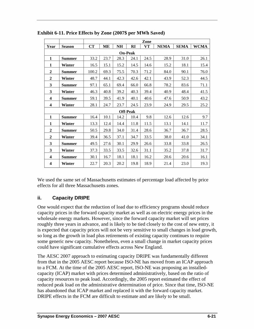
Synapse Energy Economics – 2007 AESC 6-21
Exhibit 6-11. Price Effects by Zone (2007$ per MWh Saved)
Zone Year Season CT ME NH RI VT NEMA SEMA WCMA
On-Peak 1 Summer 33.2 23.7 28.3 24.1 24.5 28.9 31.0 26.1 1 Winter 16.5 15.1 15.2 14.5 14.6 15.2 18.1 15.4 2 Summer 100.2 69.3 75.5 70.3 71.2 84.0 90.1 76.0 2 Winter 48.7 44.1 42.3 42.6 42.1 43.9 52.3 44.5 3 Summer 97.1 65.1 69.4 66.0 66.8 78.2 83.6 71.1 3 Winter 46.3 40.8 39.2 40.3 39.4 40.9 48.4 41.5 4 Summer 59.1 39.5 41.9 40.1 40.6 47.6 50.9 43.2 4 Winter 28.1 24.7 23.7 24.5 23.9 24.9 29.5 25.2
Off-Peak 1 Summer 16.4 10.1 14.2 10.4 9.8 12.6 12.6 9.7 1 Winter 13.3 12.4 14.4 11.8 11.5 13.1 14.1 11.7 2 Summer 50.5 29.8 34.0 31.4 28.6 36.7 36.7 28.5 2 Winter 39.4 36.5 37.1 34.7 33.5 38.0 41.0 34.1 3 Summer 49.5 27.6 30.1 29.9 26.6 33.8 33.8 26.5 3 Winter 37.3 33.5 33.5 32.6 31.1 35.2 37.8 31.7 4 Summer 30.1 16.7 18.1 18.1 16.2 20.6 20.6 16.1 4 Winter 22.7 20.3 20.2 19.8 18.9 21.4 23.0 19.3
We used the same set of Massachusetts estimates of percentage load affected by price effects for all three Massachusetts zones.
ii. Capacity DRIPE
One would expect that the reduction of load due to efficiency programs should reduce capacity prices in the forward capacity market as well as on electric energy prices in the wholesale energy markets. However, since the forward capacity market will set prices roughly three years in advance, and is likely to be tied closely to the cost of new entry, it is expected that capacity prices will not be very sensitive to small changes in load growth, so long as the growth in load plus retirements of existing capacity continues to require some generic new capacity. Nonetheless, even a small change in market capacity prices could have significant cumulative effects across New England.
The AESC 2007 approach to estimating capacity DRIPE was fundamentally different from that in the 2005 AESC report because ISO-NE has moved from an ICAP approach to a FCM. At the time of the 2005 AESC report, ISO-NE was proposing an installed-capacity (ICAP) market with prices determined administratively, based on the ratio of capacity resources to peak load. Accordingly, the 2005 report estimated the effect of reduced peak load on the administrative determination of price. Since that time, ISO-NE has abandoned that ICAP market and replaced it with the forward capacity market. DRIPE effects in the FCM are difficult to estimate and are likely to be small.
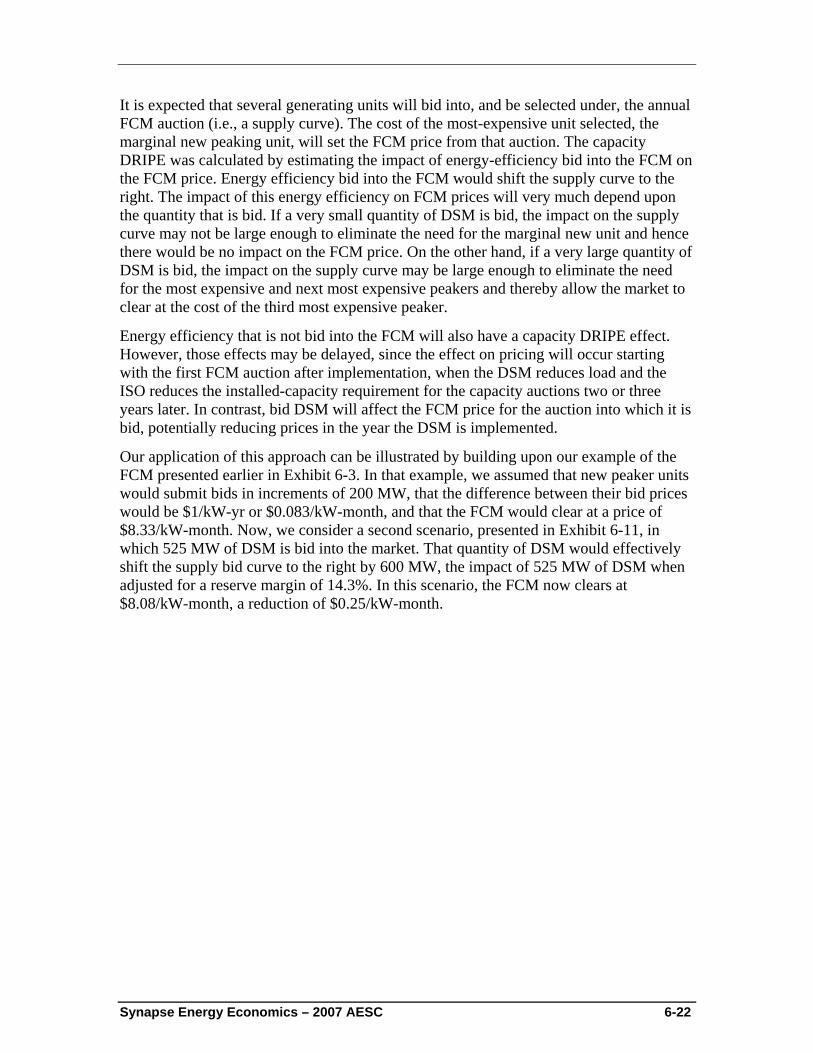
Synapse Energy Economics – 2007 AESC 6-22
It is expected that several generating units will bid into, and be selected under, the annual FCM auction (i.e., a supply curve). The cost of the most-expensive unit selected, the marginal new peaking unit, will set the FCM price from that auction. The capacity DRIPE was calculated by estimating the impact of energy-efficiency bid into the FCM on the FCM price. Energy efficiency bid into the FCM would shift the supply curve to the right. The impact of this energy efficiency on FCM prices will very much depend upon the quantity that is bid. If a very small quantity of DSM is bid, the impact on the supply curve may not be large enough to eliminate the need for the marginal new unit and hence there would be no impact on the FCM price. On the other hand, if a very large quantity of DSM is bid, the impact on the supply curve may be large enough to eliminate the need for the most expensive and next most expensive peakers and thereby allow the market to clear at the cost of the third most expensive peaker.
Energy efficiency that is not bid into the FCM will also have a capacity DRIPE effect. However, those effects may be delayed, since the effect on pricing will occur starting with the first FCM auction after implementation, when the DSM reduces load and the ISO reduces the installed-capacity requirement for the capacity auctions two or three years later. In contrast, bid DSM will affect the FCM price for the auction into which it is bid, potentially reducing prices in the year the DSM is implemented.
Our application of this approach can be illustrated by building upon our example of the FCM presented earlier in Exhibit 6-3. In that example, we assumed that new peaker units would submit bids in increments of 200 MW, that the difference between their bid prices would be $1/kW-yr or $0.083/kW-month, and that the FCM would clear at a price of $8.33/kW-month. Now, we consider a second scenario, presented in Exhibit 6-11, in which 525 MW of DSM is bid into the market. That quantity of DSM would effectively shift the supply bid curve to the right by 600 MW, the impact of 525 MW of DSM when adjusted for a reserve margin of 14.3%. In this scenario, the FCM now clears at $8.08/kW-month, a reduction of $0.25/kW-month.
Synapse Energy Economics – 2007 AESC 6-23
Exhibit 6-12. Illustrative FCM Price with 525 MW of DSM Bids
$3.00
$4.00
$5.00
$6.00
$7.00
$8.00
$9.00
20,000 22,000 24,000 26,000 28,000 30,000 32,000
MW bid
FCM
in $
/kW
-mon
th
Cumulative SupplyBids
Installed CapacityRequirement
Cumulative SupplyBids +525 MW ofDSM
New Lower Forecast Market Price
Existing MW - Price TakersNew Peakers
Existing MW bidders + 525 MW DSM
Bidd
Based upon these assumptions, each MW of DSM bid into the market would reduce the market-clearing price by an average of $0.0057/MW-year.105 Thus, each kW of DSM would reduce the market-clearing price by an average of $0.0000057/kW-year. That seems like a minute effect, but it would reduce the price of some 33,000 MW of pool-wide capacity requirement by 2011, for a total potential DRIPE effect of about $190/kW-year of load reduction.106 We recommend that this estimate be updated by analyzing actual bids once ISO-NE releases the bids received in the FCM auction in 2008.
For the 2008 DSM program year, assuming that the savings are bid into the first FCM auction in February 2008, the capacity DRIPE effect would apply to the power year starting June 2010. Since that effect would only apply to seven months in 2010, and since the analysis that produced the Share of Power Supply Exposed to Market Prices exhibit above suggests that about 65% of ISO load (between the second and third-year results) would be exposed to the market 2½ years into the future, the capacity DRIPE for 2010 might be about $72/kW of load reduction in the 2008 program plan.107 For 2011, capacity DRIPE might rise to $140/kW for a full year of FCM with less supply (about 25%) under contract.108 The impacts of efficiency implemented under the 2009 DSM program year would be similar.
105 $1/kW-yr ÷ 525 MW = $0.0057/kW-yr per MW of load reduction. We divide by 525 MW, because 175
MW of load reduction, when grossed up by a reserve margin of 14.3%, would avoid the need for 600MW or 3 peakers at 200 MW each.
106 33,000,000 kW × $0.000057/kW–yr per kW of load reduction = $190/kW of load reduction. 107 $190/kW × 65% × 7/12 = $72/kW 108 $190/kW-yr × 75% = $140/kW-yr.
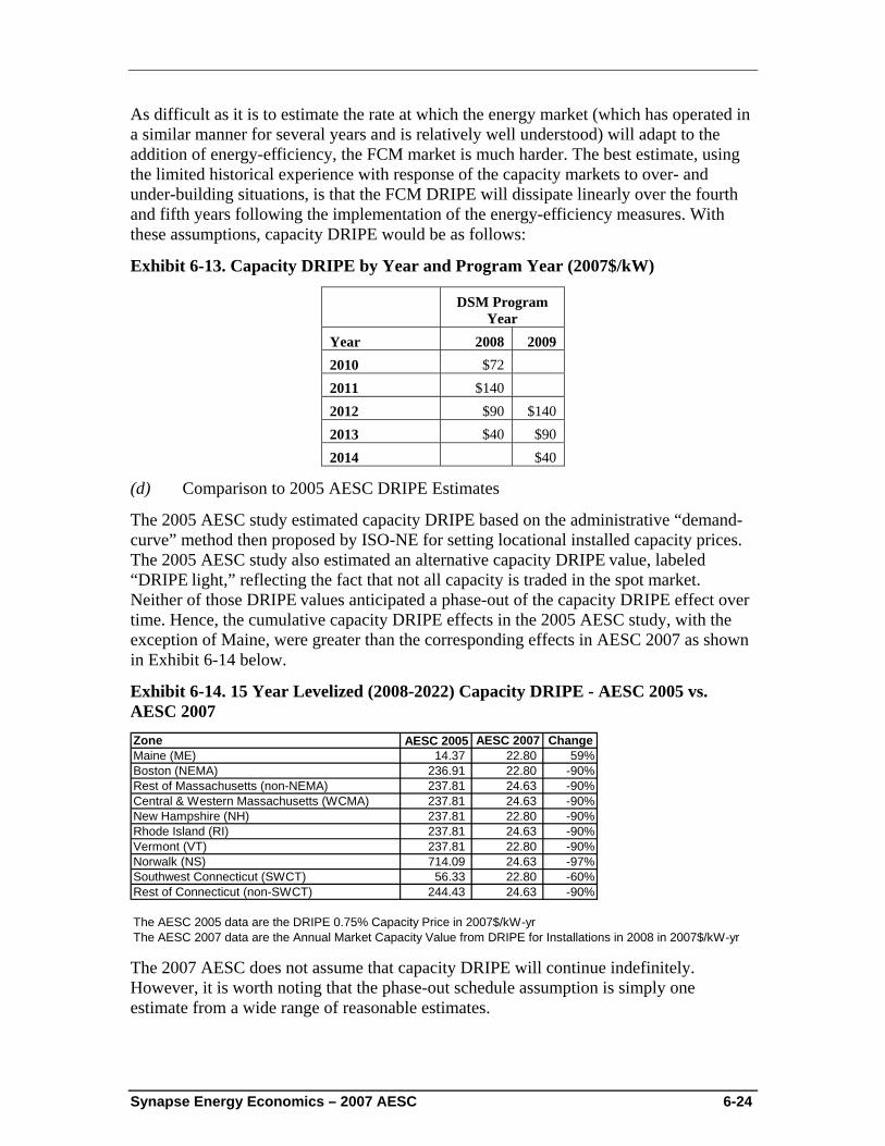
Synapse Energy Economics – 2007 AESC 6-24
As difficult as it is to estimate the rate at which the energy market (which has operated in a similar manner for several years and is relatively well understood) will adapt to the addition of energy-efficiency, the FCM market is much harder. The best estimate, using the limited historical experience with response of the capacity markets to over- and under-building situations, is that the FCM DRIPE will dissipate linearly over the fourth and fifth years following the implementation of the energy-efficiency measures. With these assumptions, capacity DRIPE would be as follows:
Exhibit 6-13. Capacity DRIPE by Year and Program Year (2007$/kW)
DSM Program Year
Year 2008 2009 2010 $72 2011 $140 2012 $90 $140 2013 $40 $90 2014 $40
(d) Comparison to 2005 AESC DRIPE Estimates
The 2005 AESC study estimated capacity DRIPE based on the administrative “demand-curve” method then proposed by ISO-NE for setting locational installed capacity prices. The 2005 AESC study also estimated an alternative capacity DRIPE value, labeled “DRIPE light,” reflecting the fact that not all capacity is traded in the spot market. Neither of those DRIPE values anticipated a phase-out of the capacity DRIPE effect over time. Hence, the cumulative capacity DRIPE effects in the 2005 AESC study, with the exception of Maine, were greater than the corresponding effects in AESC 2007 as shown in Exhibit 6-14 below.
Exhibit 6-14. 15 Year Levelized (2008-2022) Capacity DRIPE - AESC 2005 vs. AESC 2007 Zone AESC 2005 AESC 2007 ChangeMaine (ME) 14.37 22.80 59%Boston (NEMA) 236.91 22.80 -90%Rest of Massachusetts (non-NEMA) 237.81 24.63 -90%Central & Western Massachusetts (WCMA) 237.81 24.63 -90%New Hampshire (NH) 237.81 22.80 -90%Rhode Island (RI) 237.81 24.63 -90%Vermont (VT) 237.81 22.80 -90%Norwalk (NS) 714.09 24.63 -97%Southwest Connecticut (SWCT) 56.33 22.80 -60%Rest of Connecticut (non-SWCT) 244.43 24.63 -90%
The AESC 2005 data are the DRIPE 0.75% Capacity Price in 2007$/kW-yrThe AESC 2007 data are the Annual Market Capacity Value from DRIPE for Installations in 2008 in 2007$/kW-yr The 2007 AESC does not assume that capacity DRIPE will continue indefinitely. However, it is worth noting that the phase-out schedule assumption is simply one estimate from a wide range of reasonable estimates.
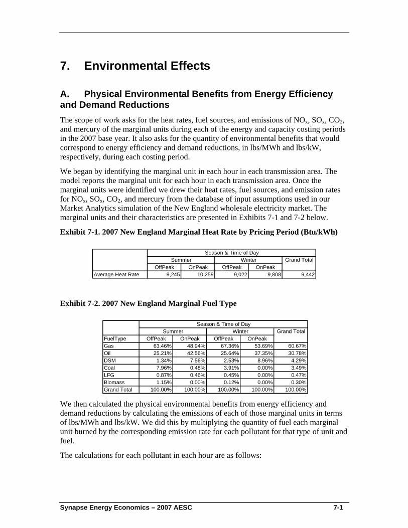
Synapse Energy Economics – 2007 AESC 7-1
7. Environmental Effects
A. Physical Environmental Benefits from Energy Efficiency and Demand Reductions The scope of work asks for the heat rates, fuel sources, and emissions of NOx, SOx, CO2, and mercury of the marginal units during each of the energy and capacity costing periods in the 2007 base year. It also asks for the quantity of environmental benefits that would correspond to energy efficiency and demand reductions, in lbs/MWh and lbs/kW, respectively, during each costing period.
We began by identifying the marginal unit in each hour in each transmission area. The model reports the marginal unit for each hour in each transmission area. Once the marginal units were identified we drew their heat rates, fuel sources, and emission rates for NOx, SOx, CO2, and mercury from the database of input assumptions used in our Market Analytics simulation of the New England wholesale electricity market. The marginal units and their characteristics are presented in Exhibits 7-1 and 7-2 below.
Exhibit 7-1. 2007 New England Marginal Heat Rate by Pricing Period (Btu/kWh)
OffPeak OnPeak OffPeak OnPeakAverage Heat Rate 9,245 10,259 9,022 9,808 9,442
Summer Winter Grand TotalSeason & Time of Day
Exhibit 7-2. 2007 New England Marginal Fuel Type
FuelType OffPeak OnPeak OffPeak OnPeakGas 63.46% 48.94% 67.36% 53.69% 60.67%Oil 25.21% 42.56% 25.64% 37.35% 30.78%DSM 1.34% 7.56% 2.53% 8.96% 4.29%Coal 7.96% 0.48% 3.91% 0.00% 3.49%LFG 0.87% 0.46% 0.45% 0.00% 0.47%Biomass 1.15% 0.00% 0.12% 0.00% 0.30%Grand Total 100.00% 100.00% 100.00% 100.00% 100.00%
Grand TotalWinterSummerSeason & Time of Day
We then calculated the physical environmental benefits from energy efficiency and demand reductions by calculating the emissions of each of those marginal units in terms of lbs/MWh and lbs/kW. We did this by multiplying the quantity of fuel each marginal unit burned by the corresponding emission rate for each pollutant for that type of unit and fuel.
The calculations for each pollutant in each hour are as follows:
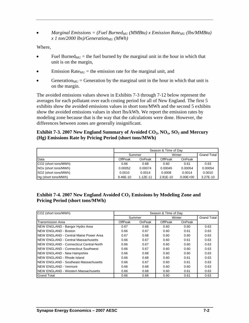
Synapse Energy Economics – 2007 AESC 7-2
• Marginal Emissions = (Fuel BurnedMU (MMBtu) x Emission RateMU (lbs/MMBtu) x 1 ton/2000 lbs)/GenerationMU (MWh)
Where,
• Fuel BurnedMU = the fuel burned by the marginal unit in the hour in which that unit is on the margin,
• Emission RateMU = the emission rate for the marginal unit, and
• GenerationMU = Generation by the marginal unit in the hour in which that unit is on the margin.
The avoided emissions values shown in Exhibits 7-3 through 7-12 below represent the averages for each pollutant over each costing period for all of New England. The first 5 exhibits show the avoided emissions values in short tons/MWh and the second 5 exhibits show the avoided emissions values in short lbs/kWh. We report the emission rates by modeling zone because that is the way that the calculations were done. However, the differences between zones are generally insignificant.
Exhibit 7-3. 2007 New England Summary of Avoided CO2, NOx, SO2 and Mercury (Hg) Emissions Rate by Pricing Period (short tons/MWh)
Grand TotalData OffPeak OnPeak OffPeak OnPeakCO2 (short tons/MWh) 0.66 0.68 0.60 0.61 0.63NOx (short tons/MWh) 0.00052 0.00074 0.00045 0.00054 0.00054SO2 (short tons/MWh) 0.0010 0.0014 0.0008 0.0014 0.0010Hg (short tons/MWh) 9.46E-10 1.12E-11 2.81E-10 0.00E+00 3.27E-10
Summer WinterSeason & Time of Day
Exhibit 7-4. 2007 New England Avoided CO2 Emissions by Modeling Zone and Pricing Period (short tons/MWh)
CO2 (short tons/MWh)Grand Total
Transmission Area OffPeak OnPeak OffPeak OnPeakNEW ENGLAND - Bangor Hydro Area 0.67 0.68 0.60 0.60 0.63NEW ENGLAND - Boston 0.66 0.67 0.60 0.61 0.63NEW ENGLAND - Central Maine Power Area 0.67 0.68 0.60 0.60 0.63NEW ENGLAND - Central Massachusetts 0.66 0.67 0.60 0.61 0.63NEW ENGLAND - Connecticut Central-North 0.66 0.67 0.60 0.60 0.63NEW ENGLAND - Connecticut Southwest 0.66 0.67 0.60 0.60 0.63NEW ENGLAND - New Hampshire 0.66 0.68 0.60 0.60 0.63NEW ENGLAND - Rhode Island 0.66 0.68 0.60 0.61 0.63NEW ENGLAND - Southeast Massachusetts 0.66 0.67 0.60 0.61 0.63NEW ENGLAND - Vermont 0.66 0.68 0.60 0.60 0.63NEW ENGLAND - Western Massachusetts 0.66 0.68 0.60 0.61 0.63Grand Total 0.66 0.68 0.60 0.61 0.63
Summer WinterSeason & Time of Day
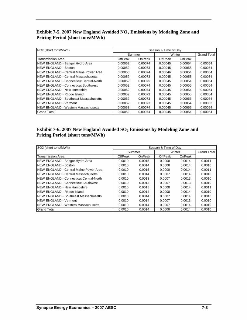
Synapse Energy Economics – 2007 AESC 7-3
Exhibit 7-5. 2007 New England Avoided NOx Emissions by Modeling Zone and Pricing Period (short tons/MWh)
NOx (short tons/MWh)Grand Total
Transmission Area OffPeak OnPeak OffPeak OnPeakNEW ENGLAND - Bangor Hydro Area 0.00053 0.00074 0.00045 0.00054 0.00054NEW ENGLAND - Boston 0.00052 0.00073 0.00045 0.00055 0.00054NEW ENGLAND - Central Maine Power Area 0.00053 0.00074 0.00046 0.00054 0.00054NEW ENGLAND - Central Massachusetts 0.00052 0.00073 0.00045 0.00055 0.00054NEW ENGLAND - Connecticut Central-North 0.00052 0.00075 0.00045 0.00054 0.00054NEW ENGLAND - Connecticut Southwest 0.00052 0.00074 0.00045 0.00055 0.00054NEW ENGLAND - New Hampshire 0.00052 0.00074 0.00045 0.00054 0.00054NEW ENGLAND - Rhode Island 0.00052 0.00073 0.00045 0.00055 0.00054NEW ENGLAND - Southeast Massachusetts 0.00052 0.00073 0.00045 0.00055 0.00054NEW ENGLAND - Vermont 0.00052 0.00073 0.00045 0.00054 0.00053NEW ENGLAND - Western Massachusetts 0.00053 0.00074 0.00045 0.00055 0.00054Grand Total 0.00052 0.00074 0.00045 0.00054 0.00054
Summer WinterSeason & Time of Day
Exhibit 7-6. 2007 New England Avoided SO2 Emissions by Modeling Zone and Pricing Period (short tons/MWh)
SO2 (short tons/MWh)Grand Total
Transmission Area OffPeak OnPeak OffPeak OnPeakNEW ENGLAND - Bangor Hydro Area 0.0010 0.0015 0.0008 0.0014 0.0011NEW ENGLAND - Boston 0.0010 0.0014 0.0008 0.0014 0.0010NEW ENGLAND - Central Maine Power Area 0.0010 0.0015 0.0008 0.0014 0.0011NEW ENGLAND - Central Massachusetts 0.0010 0.0014 0.0007 0.0014 0.0010NEW ENGLAND - Connecticut Central-North 0.0010 0.0013 0.0007 0.0013 0.0010NEW ENGLAND - Connecticut Southwest 0.0010 0.0013 0.0007 0.0013 0.0010NEW ENGLAND - New Hampshire 0.0010 0.0015 0.0008 0.0014 0.0011NEW ENGLAND - Rhode Island 0.0010 0.0014 0.0008 0.0014 0.0010NEW ENGLAND - Southeast Massachusetts 0.0010 0.0014 0.0007 0.0014 0.0010NEW ENGLAND - Vermont 0.0010 0.0014 0.0007 0.0013 0.0010NEW ENGLAND - Western Massachusetts 0.0010 0.0014 0.0007 0.0014 0.0010Grand Total 0.0010 0.0014 0.0008 0.0014 0.0010
Summer WinterSeason & Time of Day
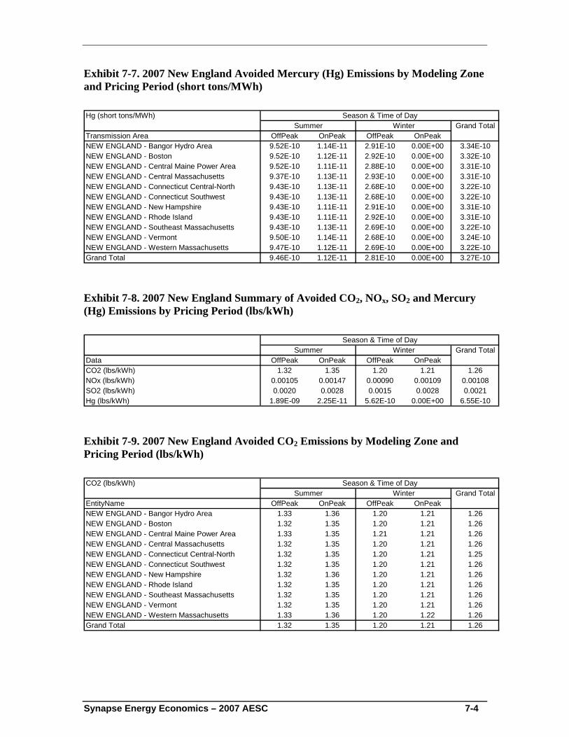
Synapse Energy Economics – 2007 AESC 7-4
Exhibit 7-7. 2007 New England Avoided Mercury (Hg) Emissions by Modeling Zone and Pricing Period (short tons/MWh)
Hg (short tons/MWh)Grand Total
Transmission Area OffPeak OnPeak OffPeak OnPeakNEW ENGLAND - Bangor Hydro Area 9.52E-10 1.14E-11 2.91E-10 0.00E+00 3.34E-10NEW ENGLAND - Boston 9.52E-10 1.12E-11 2.92E-10 0.00E+00 3.32E-10NEW ENGLAND - Central Maine Power Area 9.52E-10 1.11E-11 2.88E-10 0.00E+00 3.31E-10NEW ENGLAND - Central Massachusetts 9.37E-10 1.13E-11 2.93E-10 0.00E+00 3.31E-10NEW ENGLAND - Connecticut Central-North 9.43E-10 1.13E-11 2.68E-10 0.00E+00 3.22E-10NEW ENGLAND - Connecticut Southwest 9.43E-10 1.13E-11 2.68E-10 0.00E+00 3.22E-10NEW ENGLAND - New Hampshire 9.43E-10 1.11E-11 2.91E-10 0.00E+00 3.31E-10NEW ENGLAND - Rhode Island 9.43E-10 1.11E-11 2.92E-10 0.00E+00 3.31E-10NEW ENGLAND - Southeast Massachusetts 9.43E-10 1.13E-11 2.69E-10 0.00E+00 3.22E-10NEW ENGLAND - Vermont 9.50E-10 1.14E-11 2.68E-10 0.00E+00 3.24E-10NEW ENGLAND - Western Massachusetts 9.47E-10 1.12E-11 2.69E-10 0.00E+00 3.22E-10Grand Total 9.46E-10 1.12E-11 2.81E-10 0.00E+00 3.27E-10
Summer WinterSeason & Time of Day
Exhibit 7-8. 2007 New England Summary of Avoided CO2, NOx, SO2 and Mercury (Hg) Emissions by Pricing Period (lbs/kWh)
Grand TotalData OffPeak OnPeak OffPeak OnPeakCO2 (lbs/kWh) 1.32 1.35 1.20 1.21 1.26NOx (lbs/kWh) 0.00105 0.00147 0.00090 0.00109 0.00108SO2 (lbs/kWh) 0.0020 0.0028 0.0015 0.0028 0.0021Hg (lbs/kWh) 1.89E-09 2.25E-11 5.62E-10 0.00E+00 6.55E-10
Season & Time of DaySummer Winter
Exhibit 7-9. 2007 New England Avoided CO2 Emissions by Modeling Zone and Pricing Period (lbs/kWh)
CO2 (lbs/kWh)Grand Total
EntityName OffPeak OnPeak OffPeak OnPeakNEW ENGLAND - Bangor Hydro Area 1.33 1.36 1.20 1.21 1.26NEW ENGLAND - Boston 1.32 1.35 1.20 1.21 1.26NEW ENGLAND - Central Maine Power Area 1.33 1.35 1.21 1.21 1.26NEW ENGLAND - Central Massachusetts 1.32 1.35 1.20 1.21 1.26NEW ENGLAND - Connecticut Central-North 1.32 1.35 1.20 1.21 1.25NEW ENGLAND - Connecticut Southwest 1.32 1.35 1.20 1.21 1.26NEW ENGLAND - New Hampshire 1.32 1.36 1.20 1.21 1.26NEW ENGLAND - Rhode Island 1.32 1.35 1.20 1.21 1.26NEW ENGLAND - Southeast Massachusetts 1.32 1.35 1.20 1.21 1.26NEW ENGLAND - Vermont 1.32 1.35 1.20 1.21 1.26NEW ENGLAND - Western Massachusetts 1.33 1.36 1.20 1.22 1.26Grand Total 1.32 1.35 1.20 1.21 1.26
Season & Time of DaySummer Winter
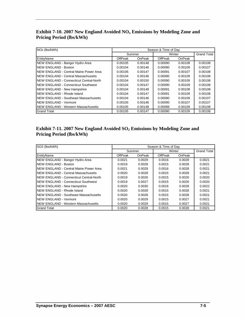
Synapse Energy Economics – 2007 AESC 7-5
Exhibit 7-10. 2007 New England Avoided NOx Emissions by Modeling Zone and Pricing Period (lbs/kWh)
NOx (lbs/kWh)Grand Total
EntityName OffPeak OnPeak OffPeak OnPeakNEW ENGLAND - Bangor Hydro Area 0.00105 0.00148 0.00090 0.00108 0.00108NEW ENGLAND - Boston 0.00104 0.00146 0.00090 0.00109 0.00107NEW ENGLAND - Central Maine Power Area 0.00105 0.00147 0.00091 0.00107 0.00108NEW ENGLAND - Central Massachusetts 0.00104 0.00146 0.00090 0.00109 0.00108NEW ENGLAND - Connecticut Central-North 0.00104 0.00150 0.00090 0.00109 0.00108NEW ENGLAND - Connecticut Southwest 0.00104 0.00147 0.00090 0.00109 0.00108NEW ENGLAND - New Hampshire 0.00104 0.00148 0.00091 0.00108 0.00108NEW ENGLAND - Rhode Island 0.00104 0.00147 0.00091 0.00109 0.00108NEW ENGLAND - Southeast Massachusetts 0.00104 0.00146 0.00090 0.00109 0.00107NEW ENGLAND - Vermont 0.00105 0.00146 0.00090 0.00107 0.00107NEW ENGLAND - Western Massachusetts 0.00105 0.00148 0.00089 0.00109 0.00108Grand Total 0.00105 0.00147 0.00090 0.00109 0.00108
WinterSeason & Time of Day
Summer
Exhibit 7-11. 2007 New England Avoided SO2 Emissions by Modeling Zone and Pricing Period (lbs/kWh)
SO2 (lbs/kWh)Grand Total
EntityName OffPeak OnPeak OffPeak OnPeakNEW ENGLAND - Bangor Hydro Area 0.0021 0.0029 0.0016 0.0028 0.0021NEW ENGLAND - Boston 0.0019 0.0028 0.0015 0.0028 0.0021NEW ENGLAND - Central Maine Power Area 0.0021 0.0029 0.0016 0.0028 0.0021NEW ENGLAND - Central Massachusetts 0.0020 0.0028 0.0015 0.0028 0.0021NEW ENGLAND - Connecticut Central-North 0.0019 0.0026 0.0015 0.0026 0.0020NEW ENGLAND - Connecticut Southwest 0.0019 0.0027 0.0015 0.0026 0.0020NEW ENGLAND - New Hampshire 0.0020 0.0030 0.0016 0.0028 0.0022NEW ENGLAND - Rhode Island 0.0020 0.0028 0.0015 0.0028 0.0021NEW ENGLAND - Southeast Massachusetts 0.0020 0.0028 0.0015 0.0028 0.0021NEW ENGLAND - Vermont 0.0020 0.0029 0.0015 0.0027 0.0021NEW ENGLAND - Western Massachusetts 0.0020 0.0029 0.0015 0.0027 0.0021Grand Total 0.0020 0.0028 0.0015 0.0028 0.0021
Season & Time of DaySummer Winter

Synapse Energy Economics – 2007 AESC 7-6
Exhibit 7-12. 2007 New England Avoided Mercury (Hg) Emissions by Modeling Zone and Pricing Period (lbs/kWh)
Hg (lbs/kWh)Grand Total
EntityName OffPeak OnPeak OffPeak OnPeakNEW ENGLAND - Bangor Hydro Area 1.90E-09 2.27E-11 5.81E-10 0.00E+00 6.68E-10NEW ENGLAND - Boston 1.90E-09 2.24E-11 5.84E-10 0.00E+00 6.65E-10NEW ENGLAND - Central Maine Power Area 1.90E-09 2.23E-11 5.76E-10 0.00E+00 6.62E-10NEW ENGLAND - Central Massachusetts 1.87E-09 2.26E-11 5.87E-10 0.00E+00 6.62E-10NEW ENGLAND - Connecticut Central-North 1.89E-09 2.26E-11 5.36E-10 0.00E+00 6.43E-10NEW ENGLAND - Connecticut Southwest 1.89E-09 2.25E-11 5.36E-10 0.00E+00 6.43E-10NEW ENGLAND - New Hampshire 1.89E-09 2.23E-11 5.83E-10 0.00E+00 6.61E-10NEW ENGLAND - Rhode Island 1.89E-09 2.23E-11 5.84E-10 0.00E+00 6.61E-10NEW ENGLAND - Southeast Massachusetts 1.89E-09 2.25E-11 5.39E-10 0.00E+00 6.44E-10NEW ENGLAND - Vermont 1.90E-09 2.27E-11 5.37E-10 0.00E+00 6.48E-10NEW ENGLAND - Western Massachusetts 1.89E-09 2.24E-11 5.39E-10 0.00E+00 6.44E-10Grand Total 1.89E-09 2.25E-11 5.62E-10 0.00E+00 6.55E-10
Season & Time of DaySummer Winter
B. Monetized Emission Values The concept of “externalities” is drawn from the field of economics. Externalities are impacts from the production of a good or service that are not reflected in price of that good or service, and that are not considered in the decision to provide that good or service.109 Air pollution is a classic externality. Pollutants are released from a facility, imposing health impacts on a population, causing damage to an ecosystem, or both. The costs of those health impacts and/or ecosystem damages are not reflected in the price of the product and are not borne by the owner of the pollutant source, and are thus external to the financial decisions pertaining to the source of the pollutant.
i. History of Environmental Externalities – Policies in New England
During the early 1990s, utilities and utility regulators in many states engaged actively in efforts to quantify environmental externalities, and to incorporate consideration of those externalities into utility planning and decision-making. Several of the New England states had proceedings dealing with externalities. In Massachusetts, a pair of related dockets (DPU 89-239 and 91-131) was particularly noteworthy for their timing, litigiousness, and thoroughness. In other states the materials from, and decisions made in, the Massachusetts dockets served as a model, sometimes adapted to the local circumstances and concerns.
In Vermont, for example, the Public Service Board adopted a policy of applying a 5% percentage adder to the cost of generation and transmission resources to reflect environmental externalities and a 10% reduction to the cost of demand side management resources in evaluating resources (VT PSB Order in Docket 5270). Vermont also held a series of workshops to discuss the development of environmental externality values for
109 In economics, an externality can be positive or negative; in this discussion we are focusing on negative
externalities.

Synapse Energy Economics – 2007 AESC 7-7
Vermont, but that process did not result in a specific set of values. Instead the environmental externality values selected in Massachusetts were adopted for use in Vermont in a series of Company-specific settlement agreements.
The Massachusetts efforts to address environmental externalities will be discussed briefly here, with a focus on carbon dioxide emissions. Docket DPU 89-239 was opened to develop “Rules to Implement Integrated Resource Planning” (IRP) and included consideration of many aspects of IRP including determination and application of environmental externalities values. In its order in that docket, the Department adopted a set of dollar values for air emissions based upon testimony by Bruce Biewald, a witness for the Division of Energy Resources. The CO2 value adopted in that order was $22 per ton of CO2 (in 1989$) and was based upon a “target” approach.110
The Department of Public Utilities (DPU) in Massachusetts subsequently opened Docket DPU 91-131 specifically to examine environmental externalities. In this docket there were 25 parties, with 21 witnesses testifying over 15 hearing days. The DPU heard testimony recommending various approaches for quantifying the CO2 externality value, including Dr. William Nordhaus testifying on behalf of Massachusetts Electric Company recommending a “damage cost approach,” Bruce Biewald testifying on behalf of the Massachusetts Division of Energy Resources, and Paul Chernick testifying on behalf of Boston Gas Company, both recommending a “sustainability target approach.”
Biewald presented a report which outlined the different methods for monetizing externalities, and recommended $23 per ton of CO2 (in 1990 dollars).111
The Department’s Order in Docket DPU 91-131 was noteworthy for its foresight regarding climate change, albeit optimistic about the timing of recognition of climate change into policies and regulation in the United States. The Department, in its November 10, 1992 order, concluded:
The record in this docket indicates that the scientific community believes that continued CO2 emissions will raise global temperatures significantly, with potentially significant damage to many aspects of society. CO2 currently is not regulated in the United States, but efforts are underway in the United States and internationally to develop regulations to reduce emissions of CO2 in the atmosphere. The generation of electricity contributes significantly to the buildup of CO2 in the atmosphere. The electricity generation industry is likely to be substantially affected by efforts to regulate, tax, or otherwise limit emissions of CO2. Clearly, it would be prudent for current and future suppliers of electricity to anticipate that CO2 regulations will be promulgated in the United States and/or internationally in the future, and that such regulations will affect resource options which might be considered in IRM resource solicitations.
110 Exh. DOER-3, Exh. BB-2, p. 26. 111 “Valuation of Environmental Externalities: Sulfur Dioxide and Greenhouse Gases,” by Bruce Biewald,
Stephen Bernow, Kevin Gurney, Michael Lazarus, and Kristin Wulfsberg. Tellus Institute, December 13, 1991.
Synapse Energy Economics – 2007 AESC 7-8
The Department has recognized the large degree of uncertainty associated with estimating (1) the future damages from CO2 emissions and (2) the future costs to control or otherwise regulate CO2 emissions. The parties in this proceeding agree that estimating the net damages associated with expected global warming is fraught with uncertainty. They disagree, however, about how much uncertainty should be attached to estimates of future global warming. They disagree even more on the likely damages from future global warming. Consequently, the Department has been presented with a wide range of estimated external cost values for CO2, from a negative value to many times the current value.112
In this case, the Department will determine whether it has been demonstrated that any proposed damage estimates for CO2 are comprehensive and reliable, or, if not, are more reasonable than the Department’s current value. 113
Based on information in the record, the Department reaffirmed the CO2 value it had adopted in the previous case, $22 per ton (in 1989 dollars).114
One of the important dynamics that can be observed in the evolution of environmental policies is the time lag between (1) the recognition of an environmental or health hazard, (2) the scientific study and documentation of the impacts, (3) the development and implementation of regulations to address the harm, and (4) the adjustment of the regulations to recognize evolving understanding of the impacts and the changing political consensus. The history of acid rain regulation provides a good example of this time lag. Acid rain was recognized as early as the mid-nineteenth century in England; however, it wasn’t until the 1960s that the science and impacts of acid rain were widely studied. In 1980 Congress established a ten year research program, the National Acidic Precipitation Assessment Program to understand and quantify acid rain impacts. The Clean Air Act Amendments of 1990 included provisions for SO2 emission caps to be implemented beginning in 1995 (“phase 1”) for the largest sources, and 2000 (“phase 2”) for other sources. More recently, the Clean Air Interstate Rule, passed by Congress in March 2005, adjusts the SO2 emissions cap downward with an ultimate effect of reducing SO2 emissions about 73% from 2003 levels, in order to address severe interstate pollutant transport issues that were not effectively addressed by prior regulation.
Action to address the depletion of the stratospheric ozone layer was more rapid, demonstrating the international community’s ability to act relatively swiftly when convinced that urgent action is required. In the early 1970s two scientists identified compounds that were depleting the ozone layer; by 1985 scientists had observed and documented an “Antarctic Ozone Hole” during springtime. In 1987 international action resulted in the negotiation of the Montreal Protocol to regulate the use and production of ozone-depleting substances. In terms of climate change and carbon dioxide regulations in the United States, we are currently at the early stages of a similar ongoing and evolving
112 DPU 86-36-G, pp.86-87 113 DPU 86-36-G, pp.73-74 114 DPU 86-36-G, pp.76
Synapse Energy Economics – 2007 AESC 7-9
process. The regulatory history of acid rain and of ozone depletion contributed important foundations for efforts to regulate greenhouse gas emissions (federal government role in addressing pollution, and framework for international negotiations on pollutants, respectively).
ii. Carbon Dioxide will be the Dominant Externality from Electricity Production and Use in New England Over the Study Period
Externalities associated with electricity production and uses include a wide variety of air pollutants, water pollutants, and land use impacts. The principle air pollutants that have externalities include carbon dioxide, sulfur dioxide, nitrogen oxides and ozone, particulates, and mercury.
There have been several fairly comprehensive studies that assess the full range of environmental impacts from electricity generation and use. These include:
• Environmental Costs of Electricity, prepared by the Pace University Center for Environmental and Legal Studies: Ottinger, R, et. al,, for NYSERDA, Oceana Publications, Inc, 1990;
• The New York State Environmental Externalities Cost Study, RCG/Hagler, Bailly, Inc. and Tellus Institute, for the Empire State Electric Energy Research Corporation (ESEERCO), multiple volumes, 1994 and 1995;
• Non-Price Benefits of BECo Demand-Side Management Programs, for the Boston Edison Settlement Board, Tellus No. 93-174A, July 1994; and
• US-EC Fuel Cycle Study, by Oak Ridge National Laboratory and Resources for the Future, for the US Department of Energy and the Commission of the European Communities, multiple volumes, 1992 to 1994.
The list of externalities from energy production and use is quite long, and includes the following:
• Air emissions (including SO2, NOx, particulates, mercury, lead, other toxins, and greenhouse gases) and the associated health and ecological damages;
• Fuel cycle impacts associated with “front end” activities such as mining and transportation, and waste disposal;
• Water use and pollution;
• Land use;
• Aesthetic impacts of power plants and related facilities;
• Radiological exposures related to nuclear power plant fuel supply and operation (routine and accident scenarios); and
• Other non-environmental externalities such as economic impacts (generally focused on employment), energy security, and others.
Synapse Energy Economics – 2007 AESC 7-10
Many of these externalities have been reduced over time, as regulations limiting emission levels have forced suppliers and buyers to consider at least a portion of those costs in their production and use decisions, thereby “internalizing” a portion of those costs. For example, the Clean Air Interstate Rule, passed by Congress in March 2005, adjusts the SO2 emissions cap downward with an ultimate effect of reducing SO2 emissions about 73% from 2003 levels. The Clean Air Act and the Clean Air Interstate Rule require further reductions in emission levels over the study period. As a result, while there remain some “external costs” associated with the residual NOx and SO2 pollution, these externalities are now relatively small. In contrast, regulators are just starting to “internalize” the impacts of carbon dioxide.
It is expected that the “carbon externality” will be the dominant externality associated with marginal electricity generation in New England. This is the case for two main reasons. First, as noted above, regulations to address the greenhouse gas emissions responsible for global climate change are lagging, particularly in the United States. The damages from criteria air pollutants are relatively bounded, and to a great extent “internalized,” as a result of existing regulations. In contrast, global climate change is a problem on an unprecedented scale with far-reaching and potentially catastrophic implications. Second, New England avoided electric energy costs over the study period are likely to be dominated by natural gas-fired generation, which has minimal SO2, mercury, and particulate emissions and relatively low NOx emissions. Hence, spending extensive time reviewing the latest literature on externality values for these emissions would not be a good use of time and budget. Based on knowledge of the electric system, and review of model runs, it is believed that the dominant environmental externality in New England over the study period will be the un-internalized cost of carbon dioxide emissions. RGGI and any federal CO2 regulations will only internalize a portion of the "greenhouse gas externality," particularly in the near term.
The California PUC has directed electric companies to include a value for carbon dioxide in their avoided cost determination and long-term resource procurement. The CA PUC found:
“In terms of specific pollutants, of significant concern to regulators and the public today is the environmental damage caused by carbon dioxide (CO2) emissions—an inescapable byproduct of fossil fuel burning and by far the major contributor to greenhouse gases. Unlike other significant pollutants from power production, CO2 is currently an unpriced externality in the energy market…. CO2 is not consistently regulated at either the Federal or State levels and is not embedded in energy prices….115
For the above reasons, values were developed for the one major emission associated with avoided electricity costs for which the near-term internalized cost most significantly understates the value supported by current science.
115 R.04-04-003, Appendix B, p. 5.
Synapse Energy Economics – 2007 AESC 7-11
iii. General Approaches to Monetizing Environmental Externalities
There are various methods available for monetizing environmental externalities such as air pollution from power plants. These include various “damage costing” approaches that seek to value the damages associated with a particular externality, and various “control cost” approaches that seek to quantify the marginal cost of controlling a particular pollutant (thus internalizing a portion or all of the externality).
The “damage costing” methods generally rely on travel costs, hedonic pricing, and contingent valuation in the absence of market prices. These are forms of “implied” valuation, asking complex and hypothetical survey questions, or extrapolating from observed behavior. For example, data on how much people will spend on travel, subsistence, and equipment, can be used to measure the value of those fish, or more accurately the value of not killing fish via air pollution. Human lives are sometimes valued based upon wage differentials for jobs that expose workers to different risks of mortality. In other words, comparing two jobs, one with higher hourly pay rate and higher risk than the other can serve as a measure of the compensation that someone is “willing to accept” in order to be exposed to the risk.
There are myriad problems with these approaches, two of which will be discussed here. First, the damage costing approaches are, in the case of global climate change, simply subject to too many problematic assumptions. We do not subscribe to the view that a reasonable economic estimate of the “damages” around the world can be developed and used as a figure for the externalities associated with carbon dioxide emissions. In other words, estimating damage is a moving target – it depends upon what concentrations we ultimately reach (or what concentrations we reach and reduce from). This is exacerbated by the fact that we do not fully understand climate change, and cannot project with certainty the levels at which certain impacts will occur. A further complicating factor is that different emissions concentrations create different damages for different regions and different groups of people. Thus, such exercises, while interesting, are fraught with difficulties including: (a) identifying the categories of changes to ecosystems and societies around the planet; (b) estimating magnitudes of impacts; (c) valuing those impacts in economic terms; (d) aggregating those values across countries with different currency exchange rates and different cultures; (e) addressing the non-linear and catastrophic aspects of the climate change damage; and (f) dealing with the paradoxes and conundrums involved in applying financial discount rates to effects stretching over centuries. Second, the fact that the “regulators’ revealed preferences” approach is unavailable, as regulators have not established relevant reference points, complicates the task of determining a carbon externality cost.
The “control cost” methods generally look at the marginal cost of control. That is, the cost of control valuations look at the last (or most expensive) unit of emissions reduction required to comply with regulations. The cost of control approach can be based upon a “regulators’ revealed preference” concept. That is, if “air regulators” are requiring a particular technology with a cost per ton of $X to be installed at power plants, then this can be taken as an indication that the value of those reductions is perceived to be at or above the cost of the controls. The cost of control approach can also be based upon a “sustainability target” concept. With the sustainability target, we start with a level of
Synapse Energy Economics – 2007 AESC 7-12
damage or risk that is considered to be acceptable, and then estimate the marginal cost of achieving that target.
The “sustainability target” approach relies on the assumption that the nations of the world will not tolerate unlimited damages. It also relies partly on an expectation that policy leaders will realize that it is cheaper to reduce emissions now and achieve a sustainability target than it is not to address climate change. It is worth noting that a cost estimate based on a sustainability target will be a bit lower than a damage cost estimate because the “sustainability target” is going to be a calculus of what climate change the planet is already committed to, and what additional change we are willing to live with (again complicated by the fact that different regions will see different impacts, and have different ideas about what is dangerous and what is sustainable). While we do not use a damage cost estimate, it is informative to consider damages to get a sense of the scale of the problem. In October 2006 a major report to Prime Minister Tony Blair stated that “the benefits of strong and early action far outweigh the economic costs of not acting.” Based on its review of results from formal economic models, the Stern Review on the Economics of Climate Change estimated that in the absence of efforts to curb climate change, the overall costs and risks of climate change will be equivalent to losing at least 5% of global GDP each year, now and forever, and could be as much as 20% of GDP or more. In contrast, the Stern Review states that the costs of action – the cost of implementing actions to curb climate change – can be limited around 1% of global GDP each year.116
iv. Estimation of CO2 Environmental Costs
Based upon our review of the merits of those various approaches, we selected an approach that estimates the cost of controlling, or stabilizing, global carbon emissions at a “sustainable level” or sustainability target. To develop that estimate, the most recent science regarding the level of emissions that would be sustainable was reviewed, as well as the literature on costs of controlling emissions at that level.
The conceptual and practical challenges for estimating a carbon externality price include the following:
• The damages are very widely distributed in time (over many decades or even centuries) and space (across the globe);
• The “physical damages” include some impacts that are very difficult to quantify and value, such as flooding large land areas; changes to local climates; species range migration; increased risk of flood and drought; changes in the amount, intensity, frequency, and type of precipitation; changes in the type, frequency, and intensity of extreme weather events (such as hurricanes, heat waves, and heavy precipitation);
116 Stern, Sir Nicholas; Stern Review of the Economics of Climate Change; Cambridge University Press,
2007.
Synapse Energy Economics – 2007 AESC 7-13
• This list of “physical damages” includes some that are extremely difficult, perhaps impossible, to reasonably express in monetary terms;
• The scientific understanding of the climate change process and climate change impacts is evolving rapidly;
• There may well be reasons (not considered here) that the environmental cost value could have a shape that starts lower and increases faster, or vice versa, having to do with periods in which rates of change are most problematic;
• The scale of the impact on the world economies associated with the impacts of climate change and/or associated with the transformations of economies to reduce greenhouse gas emissions are so large that using terms and concepts such as “marginal” can be problematic; and
• The impacts of climate change are non-linear and non-continuous, including “feedback cycles” that can most reasonably be thought of in terms of thresholds beyond which there are “run away damages” such as irreversible melting of the Greenland ice sheet and the West Antarctic ice sheet, and collapse of the Atlantic thermohaline circulation – a global ocean current system that circulates warm surface waters.
Given the daunting challenge of valuing climate damages in economic terms, AESC 2007 takes a practical approach consistent with the concepts of “sustainability” and “avoidance of undue risk.” Specifically, the carbon externality can be valued by looking at the marginal costs associated with controlling total carbon emissions at, or below, the levels that avoid the major climate change risks according to current expectations.
Nonetheless, because the environmental costs of energy production and use are so significant, and because the climate change impacts associated with power plant carbon dioxide emissions are urgently important, it is worthwhile to attempt to estimate the externality price and to put it in dollar terms that can be incorporated into electric system planning.
(a) What is the Correct Level of CO2 Emissions?
In order to determine what is currently deemed a reasonable sustainability target, current science and policy was reviewed. In 1992, over 160 nations (including the United States) agreed to “to achieve stabilization of atmospheric concentrations of greenhouse gases at levels that would prevent dangerous anthropogenic (human-induced) interference with the climate system….” (United Nations Framework Convention on Climate Change or UNFCCC).117 Achieving this commitment requires determining the maximum temperature increase above which impacts are anticipated to be dangerous, the atmospheric emissions concentration that is likely to lead to that temperature increase, and the emissions pathway that is likely to limit atmospheric concentrations and temperature increase to the desired levels.
117 There are currently over 180 signatories.
Synapse Energy Economics – 2007 AESC 7-14
The definition of what level of temperature change constitutes a dangerous climate change will ultimately be established by politicians, as it requires value judgments about what impacts are tolerable regionally and globally.118 We expect that such a definition and decision will be based upon what climate science tells us about expected impacts and mitigation opportunities.
While uncertainty and research continue, a growing number of studies identify a global average temperature increase of 2oC above pre-industrial levels as the temperature above which dangerous climate impacts are likely to occur.119 Temperature increases greater than 2oC above pre-industrial levels are associated with multiple impacts including sea level rise of many meters, drought, increasing hurricane intensity, stress on and possible destruction of unique ecosystems (such as coral reefs, the Arctic, alpine regions), and increasing risk of extreme events.120 The European Union has adopted a long-term policy goal of limiting global average temperature increase to 2oC above pre-industrial levels.121
Because of multiple uncertainties, it is difficult to define with certainty what future emissions pathway is likely to avoid exceeding that temperature increase. We reviewed several sources to determine reasonable assumptions about what level of concentrations are deemed likely to achieve the sustainability target, and what emission reductions are necessary to reach those emissions levels. The Intergovernmental Panel on Climate Change’s most recent Assessment Report indicates that concentrations of 445-490 ppm CO2 equivalent correspond to 2o – 2.4oC increases above pre-industrial levels.122 A comprehensive assessment of the economics of climate change, The Stern Review, proposes a long-term goal to stabilize greenhouse gases at between the equivalent of 450 and 550 ppm CO2.123 Recent research indicates that achieving the 2oC goal likely requires stabilizing atmospheric concentrations of carbon dioxide and other heat-trapping gases near 400 ppm carbon dioxide equivalent.124
118 For multiple discussions of the issues surrounding dangerous climate change, see Schnellnhuber,
Cramer, Nakicenovic, Wigley and Yohe, editors; Avoiding Dangerous Climate Change; Cambridge University Press, 2006. This book contains the research presented at The International Symposium on Stabilisation of Greenhouse Gas Concentrations, Avoiding Dangerous Climate Change, which took place in the U.K. in 2005.
119 Mastrandrea, M. and Schneider, S.; Probabilistic Assessment of “Dangerous” Climate Change and Emissions Scenarios: Stakeholder Metrics and Overshoot Pathways; Chapter 27 in Avoiding Dangerous Climate Change; Cambridge University Press, 2006.
120 Schnellnhuber, 2006. 121 The European Union first adopted this goal in 1996 in “Communication of the Community Strategy on
Climate Change.” Council conclusions. European Council. Brussels, Council of the EU. The EU has since reiterated its long-term commitment in 2004 and 2005 (see, e.g. Council of the European Union, Presidency conclusions, March 22-23.)
122 IPCC AR4, WGIII Summary for Policy Makers, 2007. Table SPM5. 123 Stern, Sir Nicholas; Stern Review of the Economics of Climate Change; Cambridge University Press,
2007. 124 Meinshausen, M.; What Does a 2oC Target Mean for Greenhouse Gases? A Brief Analysis Based on
Multi-Gas Emission Pathways and Several Climate Sensitivity Uncertainty Estimates; Chapter 28 in Avoiding Dangerous Climate Change; Cambridge University Press, 2006.
Synapse Energy Economics – 2007 AESC 7-15
The Intergovernmental Panel on Climate Change (IPCC) indicates that reaching concentrations of 450-490ppm CO2-eq requires reduction in global CO2 emissions in 2050 of 85-50% below 2000 emissions levels. 125 The Stern Review indicates that global emissions would have to be 70% below current levels by 2050 for stabilization at 450ppm CO2-eq.126 To accomplish such stabilization, the United States and other industrialized countries would have to reduce greenhouse gas emissions on the order of 80 – 90% below 1990 levels, and developing countries would have to achieve reductions from their baseline trajectory as soon as possible.127 In the United States, several states have adopted state greenhouse gas reduction targets of 50% or more reduction from a baseline of 1990 levels or then-current levels by 2050 (California, Connecticut, Illinois, Maine, New Hampshire, New Jersey, Oregon, and Vermont). In 2001, the New England states joined with the Eastern Canadian Premiers in also adopting a long-term policy goal of reductions on the order of 75-80% of then-current emission levels.128
The sobering news is that a long term stabilization goal of even 400 ppm might not be sufficient: “while very rapid reductions can greatly reduce the level of risk, it nevertheless remains the case that, even with the strictest measures we model, the risk of exceeding the 2ºC threshold is in the order of 10 to 25 per cent.”129 Similarly, the 2ºC threshold may not be sufficient to avoid severe impacts.130
(b) What is the Cost of Stabilizing CO2 Emissions at this Sustainable Level?
There have been several efforts to estimate the costs of achieving a variety of atmospheric concentration targets. The most comprehensive effort is the work of the Intergovernmental Panel on Climate Change. The IPCC was established by the World Meteorological Organization and UNEP in 1988 to provide scientific, technical and methodological support and analysis on climate change. IPCC has issued three assessment reports on the science of climate change, climate change impacts, and on mitigation and adaptation strategies (1990, 1995, 2001), and is currently issuing its fourth assessment report. In its fourth Assessment Report, the IPCC indicates that reductions on the order of 34 gigatonnes (Gt) would be necessary to achieve an 80% reduction below current. 131 That report estimates that up to 31 Gt in reductions are available for $100/te of
125 IPCC AR4, WGIII Summary for Policy Makers, 2007. Table SPM5. 126 Stern Review, Long Executive Summary, 2007. Page xi. 127 den Elzen, M., Meinshausen, M; Multi-Gas Emission Pathways for Meeting the EU 2oC Climate
Target; Chapter 31 in Avoiding Dangerous Climate Change; Cambridge University Press, 2006. Page 306.
128 New England Governors/Eastern Canadian Premiers, Climate Change Action Plan 2001, August 2001. NEG/ECP reiterated this commitment in June 2007 through Resolution 31-1, which states, in part, that the long term reduction goals should be met by 2050.
129 Bauer and Mastrandrea; High Stakes: Designing emissions pathways to reduce the risk of dangerous climate change; Institute for Public Policy Research, U.K.; November 2006.
130 See recent research by James Hansen, Goddard Space Flight Institute – NASA’s top climate scientist. 131 2000 emissions levels were 43Gt CO2-eq. IPCC AR4, WGIII, Summary for Policy Makers, 2007. Page
11.
Synapse Energy Economics – 2007 AESC 7-16
CO2 or less (Working Group III Summary for Policy Makers). Other studies on the costs of achieving stabilization targets include the following:
• A Vattenfalls study of abatement potential estimates that about 30 Gt reduction would be necessary for stabilization at 450 ppm, and about 27Gt are available for around $50/tCO2 – so cost would go above $50/t;132
• McKinsey & Company have developed an abatement cost curve that indicates that stabilization at 450 ppm would have a marginal abatement cost of about $50/t, stabilization at 400 ppm would have a marginal abatement cost of over $60/tCO2; and
• The Stern Review itself talks primarily about macro-economic costs; however an underlying meta-analysis of modeling literature concludes that “even stringent stabilization targets can be met without materially affecting world GDP growth, at low carbon tax rates or permit prices, at least by 2030 (in $US(2000), less than $15/tCO2 for 550ppmv and $50/tCO2 for 450ppmv for CO2).”133
The IPCC Working Group III Summary for Policy Makers states on page 29 (references omitted): “An effective carbon-price signal could realize significant mitigation potential in all sectors.
• Modeling studies show carbon prices rising to 20 to 80 US$/tCOB2 B-eq by 2030 and 30 to 155 US$/tCOB2 B-eq by 2050 are consistent with stabilization at around 550 ppm COB2 B-eq by 2100. For the same stabilization level, studies since the Third Assessment Report that take into account induced technological change lower these price ranges to 5 to 65 US$/tCOB2 Beq in 2030 and 15 to 130 US$/tCOB2 B-eq in 2050.
• Most top-down, as well as some 2050 bottom-up assessments, suggest that real or implicit carbon prices of 20 to 50 US$/tCOB2 B-eq, sustained or increased over decades, could lead to a power generation sector with low-greenhouse gas emissions by 2050 and make many mitigation options in the end-use sectors economically attractive.”
Based on a review of these different sources, we believe that it is reasonable to anticipate a marginal cost of control of $60/tCO2-eq for achieving a stabilization target that is likely to avoid temperature increases higher than 2oC above pre-industrial levels. Of course, selection of this value requires multiple assumptions.
132 Vattenfalls Global Climate Impact Abatement Map, accessed May 30, 2007. 133 Barker, Terry et. al.; A report prepared for the HM Treasury Stern Review on “The economics of
climate change” The Costs of Greenhouse Gas Mitigation with Induced Technological Change: A Meta-Analysis of Estimates in the Literature; 4 CMR, University of Cambridge. July 2006.
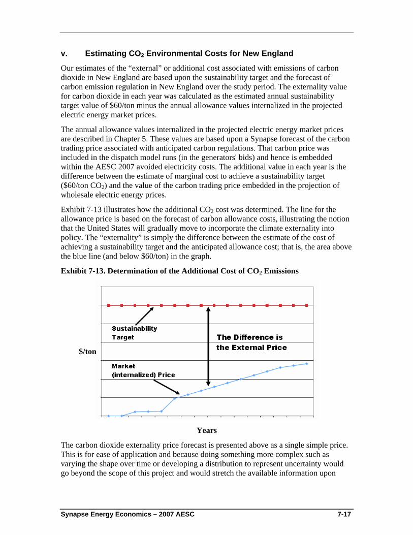
Synapse Energy Economics – 2007 AESC 7-17
v. Estimating CO2 Environmental Costs for New England
Our estimates of the “external” or additional cost associated with emissions of carbon dioxide in New England are based upon the sustainability target and the forecast of carbon emission regulation in New England over the study period. The externality value for carbon dioxide in each year was calculated as the estimated annual sustainability target value of $60/ton minus the annual allowance values internalized in the projected electric energy market prices.
The annual allowance values internalized in the projected electric energy market prices are described in Chapter 5. These values are based upon a Synapse forecast of the carbon trading price associated with anticipated carbon regulations. That carbon price was included in the dispatch model runs (in the generators' bids) and hence is embedded within the AESC 2007 avoided electricity costs. The additional value in each year is the difference between the estimate of marginal cost to achieve a sustainability target ($60/ton CO2) and the value of the carbon trading price embedded in the projection of wholesale electric energy prices.
Exhibit 7-13 illustrates how the additional CO2 cost was determined. The line for the allowance price is based on the forecast of carbon allowance costs, illustrating the notion that the United States will gradually move to incorporate the climate externality into policy. The “externality” is simply the difference between the estimate of the cost of achieving a sustainability target and the anticipated allowance cost; that is, the area above the blue line (and below $60/ton) in the graph.
Exhibit 7-13. Determination of the Additional Cost of CO2 Emissions
Years
The carbon dioxide externality price forecast is presented above as a single simple price. This is for ease of application and because doing something more complex such as varying the shape over time or developing a distribution to represent uncertainty would go beyond the scope of this project and would stretch the available information upon
$/ton
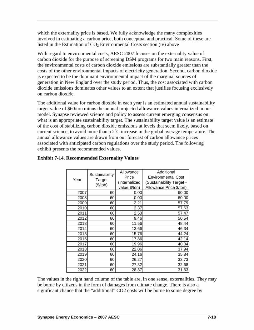
Synapse Energy Economics – 2007 AESC 7-18
which the externality price is based. We fully acknowledge the many complexities involved in estimating a carbon price, both conceptual and practical. Some of these are listed in the Estimation of CO2 Environmental Costs section (iv) above
With regard to environmental costs, AESC 2007 focuses on the externality value of carbon dioxide for the purpose of screening DSM programs for two main reasons. First, the environmental costs of carbon dioxide emissions are substantially greater than the costs of the other environmental impacts of electricity generation. Second, carbon dioxide is expected to be the dominant environmental impact of the marginal sources of generation in New England over the study period. Thus, the cost associated with carbon dioxide emissions dominates other values to an extent that justifies focusing exclusively on carbon dioxide.
The additional value for carbon dioxide in each year is an estimated annual sustainability target value of $60/ton minus the annual projected allowance values internalized in our model. Synapse reviewed science and policy to assess current emerging consensus on what is an appropriate sustainability target. The sustainability target value is an estimate of the cost of stabilizing carbon dioxide emissions at levels that seem likely, based on current science, to avoid more than a 2oC increase in the global average temperature. The annual allowance values are drawn from our forecast of carbon allowance prices associated with anticipated carbon regulations over the study period. The following exhibit presents the recommended values.
Exhibit 7-14. Recommended Externality Values
YearSustainability
Target ($/ton)
Allowance Price
(internalized value $/ton)
Additional Environmental Cost
(Sustainability Target - Allowance Price $/ton)
2007 60 0.00 60.002008 60 0.00 60.002009 60 2.21 57.792010 60 2.37 57.632011 60 2.53 57.472012 60 9.46 50.542013 60 11.56 48.442014 60 13.66 46.342015 60 15.76 44.242016 60 17.86 42.142017 60 19.96 40.042018 60 22.06 37.942019 60 24.16 35.842020 60 26.27 33.732021 60 27.32 32.682022 60 28.37 31.63
The values in the right hand column of the table are, in one sense, externalities. They may be borne by citizens in the form of damages from climate change. There is also a significant chance that the “additional” CO2 costs will be borne to some degree by
Synapse Energy Economics – 2007 AESC 7-19
electricity consumers in the form of compliance costs in electricity rates if emission regulations require greater reductions more rapidly than we have assumed.
vi. Applying CO2 Costs in Evaluations of DSM Programs
The externality values from Exhibit 7-14 are provided in the avoided electricity cost workbooks presented in Appendix E. They are expressed as $/kWh based upon our analysis of the CO2 emissions of the marginal generating units in each year of the study period.
At a minimum program administrators should calculate the costs and benefits of DSM programs without, and then with, these values in order to assess their incremental impact on the cost-effectiveness of programs. However, we recommend the program administrators include these values in their analyses of DSM, unless specifically prohibited from doing so by state or local law or regulation. The next section explains why a DSM program could result in CO2 emission reductions even under a cap and trade regulatory framework.
vii. Impact of DSM on Carbon Emissions Under a Cap and Trade Regulatory Framework
The Regional Greenhouse Gas Initiative is a cap and trade greenhouse gas program for power plants in the northeastern United States. Discussions to develop the program began in 2003, states signed a memorandum of understanding identifying the main elements of the program in December 2005, and in August 2006 they adopted a model rule for implementing the program. Currently nine states have decided to participate: Connecticut, Delaware, Maine, Massachusetts, New Hampshire, New Jersey, New York, Rhode Island, and Vermont. Maryland passed a law in April 2006 requiring participation in RGGI. Pennsylvania, the District of Columbia, the Eastern Canadian Provinces, and New Brunswick are official “observers” in the RGGI process. Individual states are now engaged in regulatory proceedings to adopt regulations consistent with the agreement.
As currently designed, the program will:
• Stabilize CO2 emissions from power plants at current levels for the period 2009-2015, followed by a 10% reduction below current levels by 2019;
• Allocate a minimum of 25% of allowances for consumer benefit and strategic energy purposes. Allowances allocated for consumer benefit will be auctioned and the proceeds of the auction used for consumer benefit and strategic energy purposes; and
• Include certain offset provisions that increase flexibility to moderate price impacts and development of complimentary energy policies to improve energy efficiency, decrease the use of higher polluting electricity generation and maintain economic growth.
Synapse Energy Economics – 2007 AESC 7-20
With carbon dioxide emissions regulated under a cap and trade system, as is assumed in this market price analysis, it is conceivable that a load reduction from a DSM program will not lead to a reduction in the amount of total system carbon dioxide emissions. The annual total system emissions for the affected facilities in the relevant region are, after all, capped. In the analysis that was documented in this report, the relevant cap and trade regulation is the Regional Greenhouse Gas Initiative (RGGI) for the period 2009 to 2012 and the assumed national cap and trade system thereafter. However, there are a number of reasons why a DSM program could result in CO2 emission reductions, specifically:
• Reduction in load that reduces the cost (marginal or total cost) of achieving an emissions cap can result in a tightening of the cap. This is a complex interaction between the energy system and political and economic systems, and is difficult or impossible to model, but the dynamic may reasonably be assumed to exist;
• Specific provisions in RGGI provide for a tightening or loosening of the cap (via adjustments to the offset provisions that are triggered at different price levels). It is unknown at this point whether and to what extent such “automatic” adjustments might be built into the US carbon regulatory system;
• It is also possible that DSM efforts will be accompanied by specific retirements or allocations of allowances that would cause them to have an impact on the overall system level of emissions (effectively tightening the cap); and
• to the extent that the cap and trade system “leaks” because of its geographic boundaries, one would expect the benefits of a carbon emissions reduction resulting from a DSM program to similarly “leak.” That is, a load reduction in New York could cause reductions in generation (and emissions) at power plants in New York, Pennsylvania, and elsewhere. Because New York is in the RGGI cap and trade system, the emissions reductions realized at New York generating units may pop up as a result of increased sales of allowances from NY to other RGGI states. But because Pennsylvania is not in the RGGI system, the emissions reductions at Pennsylvania generating units would be true reductions attributable to the DSM program.
Synapse Energy Economics – AESC 2007 A-1
Appendix A – Common Modeling Assumptions Inflation Rate
Inflation increased since the AESC 2005 study, which used a rate of 2.25%. Inflation was 3.03% in 2005 and 2.90% in 2006 as shown in the exhibit below. In addition, the twenty year average (1987-2006) derived from the chained GDP deflator was 2.47%. As a result, the long-term inflation rate used in this study was 2.50%.
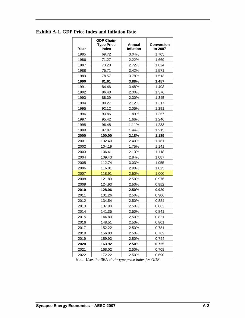
Synapse Energy Economics – AESC 2007 A-2
Exhibit A-1. GDP Price Index and Inflation Rate
Year
GDP Chain-Type Price
Index Annual Inflation
Conversion to 2007
1985 69.72 3.04% 1.705 1986 71.27 2.22% 1.669 1987 73.20 2.72% 1.624 1988 75.71 3.42% 1.571 1989 78.57 3.78% 1.513 1990 81.61 3.88% 1.457 1991 84.46 3.48% 1.408 1992 86.40 2.30% 1.376 1993 88.39 2.30% 1.345 1994 90.27 2.12% 1.317 1995 92.12 2.05% 1.291 1996 93.86 1.89% 1.267 1997 95.42 1.66% 1.246 1998 96.48 1.11% 1.233 1999 97.87 1.44% 1.215 2000 100.00 2.18% 1.189 2001 102.40 2.40% 1.161 2002 104.19 1.75% 1.141 2003 106.41 2.13% 1.118 2004 109.43 2.84% 1.087 2005 112.74 3.03% 1.055 2006 116.01 2.90% 1.025 2007 118.91 2.50% 1.000 2008 121.89 2.50% 0.976 2009 124.93 2.50% 0.952 2010 128.06 2.50% 0.929 2011 131.26 2.50% 0.906 2012 134.54 2.50% 0.884 2013 137.90 2.50% 0.862 2014 141.35 2.50% 0.841 2015 144.89 2.50% 0.821 2016 148.51 2.50% 0.801 2017 152.22 2.50% 0.781 2018 156.03 2.50% 0.762 2019 159.93 2.50% 0.744 2020 163.92 2.50% 0.725 2021 168.02 2.50% 0.708 2022 172.22 2.50% 0.690
Note: Uses the BEA chain-type price index for GDP
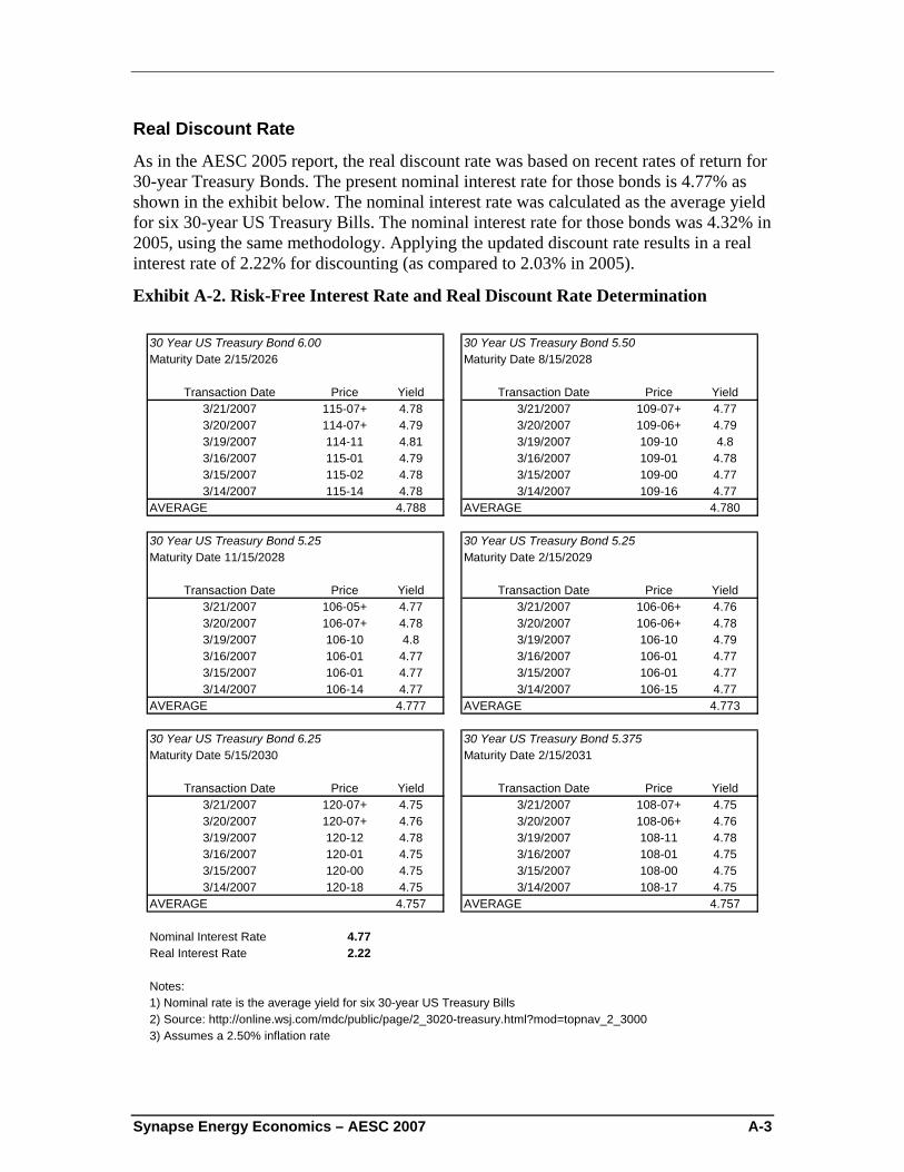
Synapse Energy Economics – AESC 2007 A-3
Real Discount Rate
As in the AESC 2005 report, the real discount rate was based on recent rates of return for 30-year Treasury Bonds. The present nominal interest rate for those bonds is 4.77% as shown in the exhibit below. The nominal interest rate was calculated as the average yield for six 30-year US Treasury Bills. The nominal interest rate for those bonds was 4.32% in 2005, using the same methodology. Applying the updated discount rate results in a real interest rate of 2.22% for discounting (as compared to 2.03% in 2005).
Exhibit A-2. Risk-Free Interest Rate and Real Discount Rate Determination
30 Year US Treasury Bond 6.00 30 Year US Treasury Bond 5.50Maturity Date 2/15/2026 Maturity Date 8/15/2028
Transaction Date Price Yield Transaction Date Price Yield3/21/2007 115-07+ 4.78 3/21/2007 109-07+ 4.773/20/2007 114-07+ 4.79 3/20/2007 109-06+ 4.793/19/2007 114-11 4.81 3/19/2007 109-10 4.83/16/2007 115-01 4.79 3/16/2007 109-01 4.783/15/2007 115-02 4.78 3/15/2007 109-00 4.773/14/2007 115-14 4.78 3/14/2007 109-16 4.77
AVERAGE 4.788 AVERAGE 4.780
30 Year US Treasury Bond 5.25 30 Year US Treasury Bond 5.25Maturity Date 11/15/2028 Maturity Date 2/15/2029
Transaction Date Price Yield Transaction Date Price Yield3/21/2007 106-05+ 4.77 3/21/2007 106-06+ 4.763/20/2007 106-07+ 4.78 3/20/2007 106-06+ 4.783/19/2007 106-10 4.8 3/19/2007 106-10 4.793/16/2007 106-01 4.77 3/16/2007 106-01 4.773/15/2007 106-01 4.77 3/15/2007 106-01 4.773/14/2007 106-14 4.77 3/14/2007 106-15 4.77
AVERAGE 4.777 AVERAGE 4.773
30 Year US Treasury Bond 6.25 30 Year US Treasury Bond 5.375Maturity Date 5/15/2030 Maturity Date 2/15/2031
Transaction Date Price Yield Transaction Date Price Yield3/21/2007 120-07+ 4.75 3/21/2007 108-07+ 4.753/20/2007 120-07+ 4.76 3/20/2007 108-06+ 4.763/19/2007 120-12 4.78 3/19/2007 108-11 4.783/16/2007 120-01 4.75 3/16/2007 108-01 4.753/15/2007 120-00 4.75 3/15/2007 108-00 4.753/14/2007 120-18 4.75 3/14/2007 108-17 4.75
AVERAGE 4.757 AVERAGE 4.757
Nominal Interest Rate 4.77 Real Interest Rate 2.22
Notes:1) Nominal rate is the average yield for six 30-year US Treasury Bills2) Source: http://online.wsj.com/mdc/public/page/2_3020-treasury.html?mod=topnav_2_30003) Assumes a 2.50% inflation rate
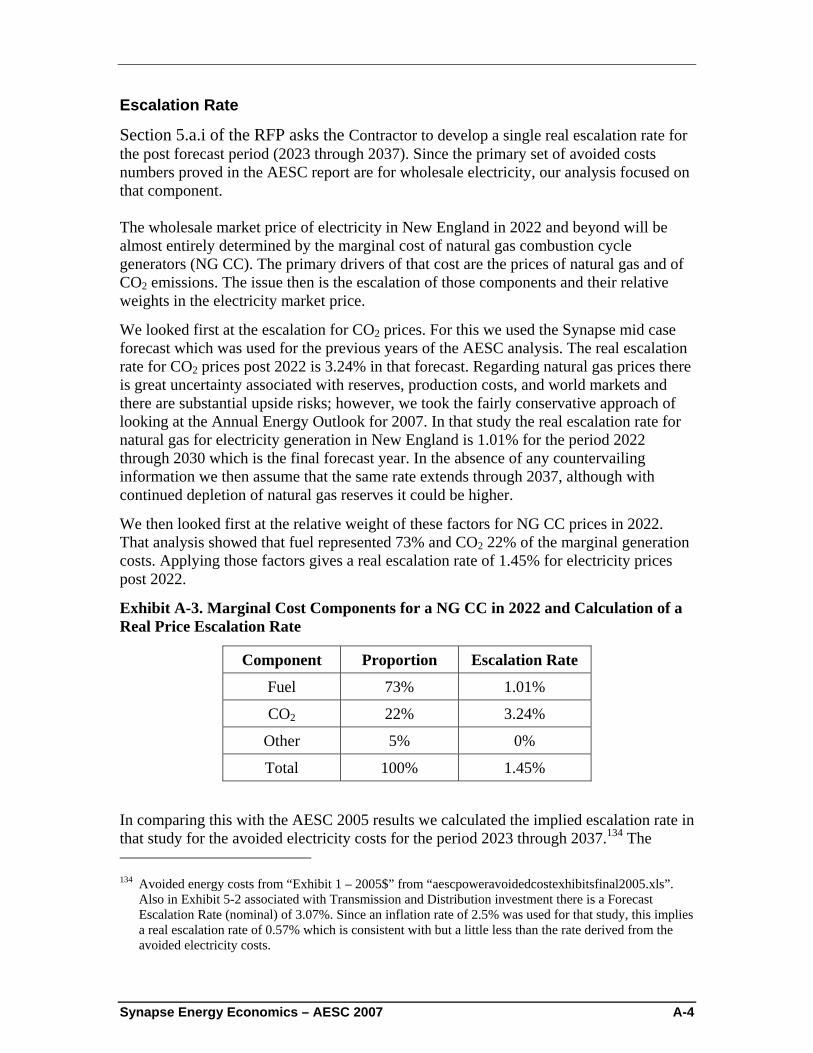
Synapse Energy Economics – AESC 2007 A-4
Escalation Rate
Section 5.a.i of the RFP asks the Contractor to develop a single real escalation rate for the post forecast period (2023 through 2037). Since the primary set of avoided costs numbers proved in the AESC report are for wholesale electricity, our analysis focused on that component. The wholesale market price of electricity in New England in 2022 and beyond will be almost entirely determined by the marginal cost of natural gas combustion cycle generators (NG CC). The primary drivers of that cost are the prices of natural gas and of CO2 emissions. The issue then is the escalation of those components and their relative weights in the electricity market price.
We looked first at the escalation for CO2 prices. For this we used the Synapse mid case forecast which was used for the previous years of the AESC analysis. The real escalation rate for CO2 prices post 2022 is 3.24% in that forecast. Regarding natural gas prices there is great uncertainty associated with reserves, production costs, and world markets and there are substantial upside risks; however, we took the fairly conservative approach of looking at the Annual Energy Outlook for 2007. In that study the real escalation rate for natural gas for electricity generation in New England is 1.01% for the period 2022 through 2030 which is the final forecast year. In the absence of any countervailing information we then assume that the same rate extends through 2037, although with continued depletion of natural gas reserves it could be higher.
We then looked first at the relative weight of these factors for NG CC prices in 2022. That analysis showed that fuel represented 73% and CO2 22% of the marginal generation costs. Applying those factors gives a real escalation rate of 1.45% for electricity prices post 2022.
Exhibit A-3. Marginal Cost Components for a NG CC in 2022 and Calculation of a Real Price Escalation Rate
Component Proportion Escalation Rate
Fuel 73% 1.01%
CO2 22% 3.24%
Other 5% 0%
Total 100% 1.45%
In comparing this with the AESC 2005 results we calculated the implied escalation rate in that study for the avoided electricity costs for the period 2023 through 2037.134 The 134 Avoided energy costs from “Exhibit 1 – 2005$” from “aescpoweravoidedcostexhibitsfinal2005.xls”.
Also in Exhibit 5-2 associated with Transmission and Distribution investment there is a Forecast Escalation Rate (nominal) of 3.07%. Since an inflation rate of 2.5% was used for that study, this implies a real escalation rate of 0.57% which is consistent with but a little less than the rate derived from the avoided electricity costs.
Synapse Energy Economics – AESC 2007 A-5
annual average real escalation rate from this calculation was 0.68%. This is significantly less than the current proposed escalation rate but does not incorporate CO2 costs and reflects a more optimistic view of future energy prices.
Although there are many uncertainties associated with energy prices this far in the future, our recommendation is a real escalation rate of 1.4% for wholesale electricity prices for 2023 through 2037.
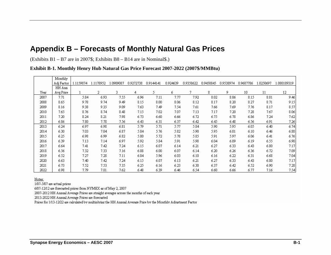
Synapse Energy Economics – AESC 2007 B-1
Appendix B – Forecasts of Monthly Natural Gas Prices (Exhibits B1 – B7 are in 2007$; Exhibits B8 – B14 are in Nominal$.)
Exhibit B-1. Monthly Henry Hub Natural Gas Price Forecast 2007-2022 (2007$/MMBtu)
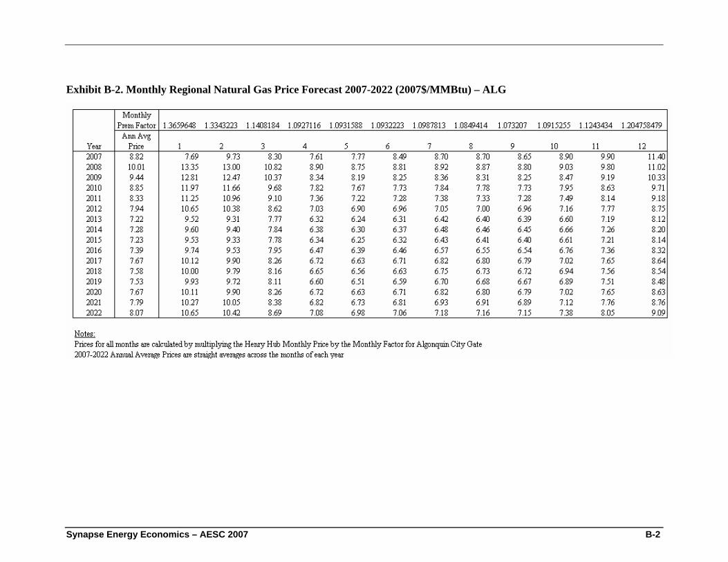
Synapse Energy Economics – AESC 2007 B-2
Exhibit B-2. Monthly Regional Natural Gas Price Forecast 2007-2022 (2007$/MMBtu) – ALG
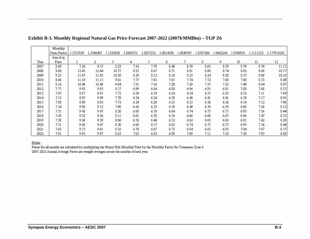
Synapse Energy Economics – AESC 2007 B-3
Exhibit B-3. Monthly Regional Natural Gas Price Forecast 2007-2022 (2007$/MMBtu) – TGP Z6
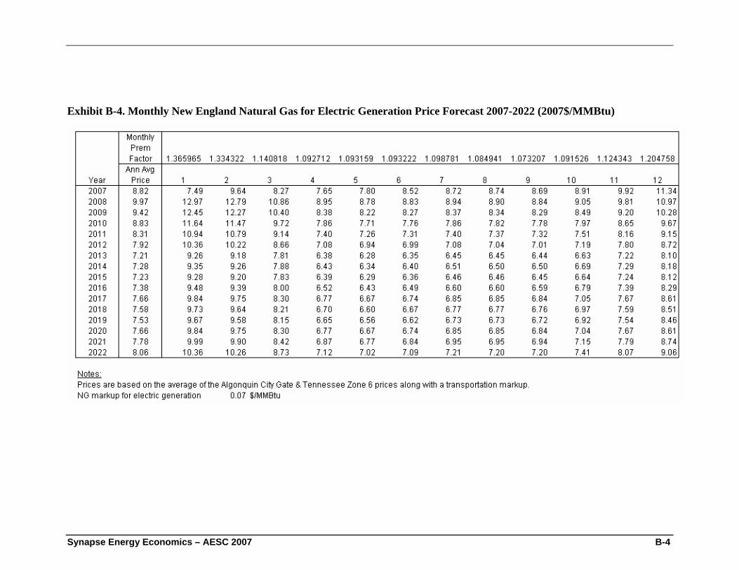
Synapse Energy Economics – AESC 2007 B-4
Exhibit B-4. Monthly New England Natural Gas for Electric Generation Price Forecast 2007-2022 (2007$/MMBtu)
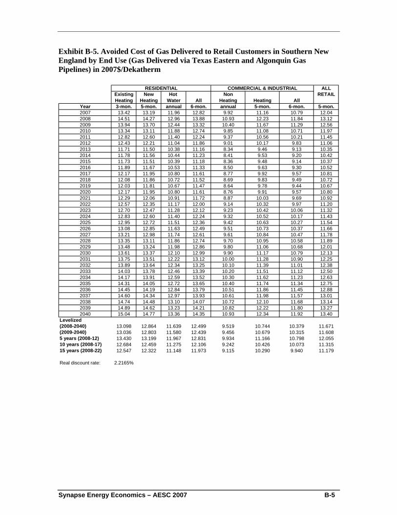
Synapse Energy Economics – AESC 2007 B-5
Exhibit B-5. Avoided Cost of Gas Delivered to Retail Customers in Southern New England by End Use (Gas Delivered via Texas Eastern and Algonquin Gas Pipelines) in 2007$/Dekatherm
ALLExisting New Hot Non RETAILHeating Heating Water All Heating Heating All
Year 3-mon. 5-mon. annual 6-mon. annual 5-mon. 6-mon. 5-mon.2007 13.42 13.19 11.96 12.82 9.92 11.16 10.79 12.042008 14.51 14.27 12.96 13.88 10.93 12.23 11.84 13.122009 13.94 13.70 12.44 13.32 10.40 11.67 11.29 12.562010 13.34 13.11 11.88 12.74 9.85 11.08 10.71 11.972011 12.82 12.60 11.40 12.24 9.37 10.56 10.21 11.452012 12.43 12.21 11.04 11.86 9.01 10.17 9.83 11.062013 11.71 11.50 10.38 11.16 8.34 9.46 9.13 10.352014 11.78 11.56 10.44 11.23 8.41 9.53 9.20 10.422015 11.73 11.51 10.39 11.18 8.36 9.48 9.14 10.372016 11.89 11.67 10.53 11.33 8.50 9.63 9.30 10.522017 12.17 11.95 10.80 11.61 8.77 9.92 9.57 10.812018 12.08 11.86 10.72 11.52 8.69 9.83 9.49 10.722019 12.03 11.81 10.67 11.47 8.64 9.78 9.44 10.672020 12.17 11.95 10.80 11.61 8.76 9.91 9.57 10.802021 12.29 12.06 10.91 11.72 8.87 10.03 9.69 10.922022 12.57 12.35 11.17 12.00 9.14 10.32 9.97 11.202023 12.70 12.47 11.28 12.12 9.23 10.42 10.06 11.322024 12.83 12.60 11.40 12.24 9.32 10.52 10.17 11.432025 12.95 12.72 11.51 12.36 9.42 10.63 10.27 11.542026 13.08 12.85 11.63 12.49 9.51 10.73 10.37 11.662027 13.21 12.98 11.74 12.61 9.61 10.84 10.47 11.782028 13.35 13.11 11.86 12.74 9.70 10.95 10.58 11.892029 13.48 13.24 11.98 12.86 9.80 11.06 10.68 12.012030 13.61 13.37 12.10 12.99 9.90 11.17 10.79 12.132031 13.75 13.51 12.22 13.12 10.00 11.28 10.90 12.252032 13.89 13.64 12.34 13.25 10.10 11.39 11.01 12.382033 14.03 13.78 12.46 13.39 10.20 11.51 11.12 12.502034 14.17 13.91 12.59 13.52 10.30 11.62 11.23 12.632035 14.31 14.05 12.72 13.65 10.40 11.74 11.34 12.752036 14.45 14.19 12.84 13.79 10.51 11.86 11.45 12.882037 14.60 14.34 12.97 13.93 10.61 11.98 11.57 13.012038 14.74 14.48 13.10 14.07 10.72 12.10 11.68 13.142039 14.89 14.62 13.23 14.21 10.82 12.22 11.80 13.272040 15.04 14.77 13.36 14.35 10.93 12.34 11.92 13.40
Levelized(2008-2040) 13.098 12.864 11.639 12.499 9.519 10.744 10.379 11.671(2009-2040) 13.036 12.803 11.580 12.439 9.456 10.679 10.315 11.6085 years (2008-12) 13.430 13.199 11.967 12.831 9.934 11.166 10.798 12.05510 years (2008-17) 12.684 12.459 11.275 12.106 9.242 10.426 10.073 11.31515 years (2008-22) 12.547 12.322 11.148 11.973 9.115 10.290 9.940 11.179
Real discount rate: 2.2165%
COMMERCIAL & INDUSTRIALRESIDENTIAL
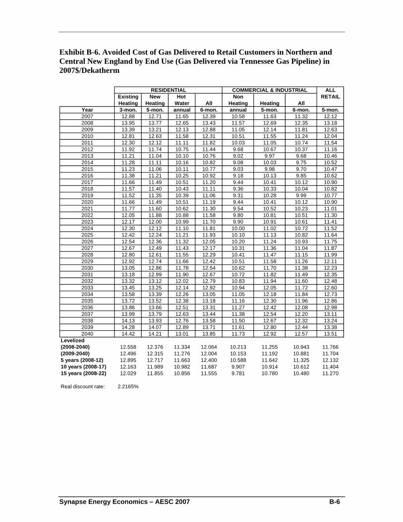
Synapse Energy Economics – AESC 2007 B-6
Exhibit B-6. Avoided Cost of Gas Delivered to Retail Customers in Northern and Central New England by End Use (Gas Delivered via Tennessee Gas Pipeline) in 2007$/Dekatherm
ALLExisting New Hot Non RETAILHeating Heating Water All Heating Heating All
Year 3-mon. 5-mon. annual 6-mon. annual 5-mon. 6-mon. 5-mon.2007 12.88 12.71 11.65 12.39 10.58 11.63 11.32 12.122008 13.95 13.77 12.65 13.43 11.57 12.69 12.35 13.182009 13.39 13.21 12.13 12.88 11.05 12.14 11.81 12.632010 12.81 12.63 11.58 12.31 10.51 11.55 11.24 12.042011 12.30 12.12 11.11 11.82 10.03 11.05 10.74 11.542012 11.92 11.74 10.75 11.44 9.68 10.67 10.37 11.162013 11.21 11.04 10.10 10.76 9.02 9.97 9.68 10.462014 11.28 11.11 10.16 10.82 9.08 10.03 9.75 10.522015 11.23 11.06 10.11 10.77 9.03 9.98 9.70 10.472016 11.38 11.21 10.25 10.92 9.18 10.13 9.85 10.622017 11.66 11.49 10.51 11.20 9.44 10.41 10.12 10.902018 11.57 11.40 10.43 11.11 9.36 10.33 10.04 10.822019 11.52 11.35 10.39 11.06 9.31 10.28 9.99 10.772020 11.66 11.49 10.51 11.19 9.44 10.41 10.12 10.902021 11.77 11.60 10.62 11.30 9.54 10.52 10.23 11.012022 12.05 11.88 10.88 11.58 9.80 10.81 10.51 11.302023 12.17 12.00 10.99 11.70 9.90 10.91 10.61 11.412024 12.30 12.12 11.10 11.81 10.00 11.02 10.72 11.522025 12.42 12.24 11.21 11.93 10.10 11.13 10.82 11.642026 12.54 12.36 11.32 12.05 10.20 11.24 10.93 11.752027 12.67 12.49 11.43 12.17 10.31 11.36 11.04 11.872028 12.80 12.61 11.55 12.29 10.41 11.47 11.15 11.992029 12.92 12.74 11.66 12.42 10.51 11.58 11.26 12.112030 13.05 12.86 11.78 12.54 10.62 11.70 11.38 12.232031 13.18 12.99 11.90 12.67 10.72 11.82 11.49 12.352032 13.32 13.12 12.02 12.79 10.83 11.94 11.60 12.482033 13.45 13.25 12.14 12.92 10.94 12.05 11.72 12.602034 13.58 13.39 12.26 13.05 11.05 12.18 11.84 12.732035 13.72 13.52 12.38 13.18 11.16 12.30 11.96 12.862036 13.86 13.66 12.51 13.31 11.27 12.42 12.08 12.982037 13.99 13.79 12.63 13.44 11.38 12.54 12.20 13.112038 14.13 13.93 12.76 13.58 11.50 12.67 12.32 13.242039 14.28 14.07 12.89 13.71 11.61 12.80 12.44 13.382040 14.42 14.21 13.01 13.85 11.73 12.92 12.57 13.51
Levelized(2008-2040) 12.558 12.376 11.334 12.064 10.213 11.255 10.943 11.766(2009-2040) 12.496 12.315 11.276 12.004 10.153 11.192 10.881 11.7045 years (2008-12) 12.895 12.717 11.663 12.400 10.588 11.642 11.325 12.13210 years (2008-17) 12.163 11.989 10.982 11.687 9.907 10.914 10.612 11.40415 years (2008-22) 12.029 11.855 10.856 11.555 9.781 10.780 10.480 11.270
Real discount rate: 2.2165%
RESIDENTIAL COMMERCIAL & INDUSTRIAL
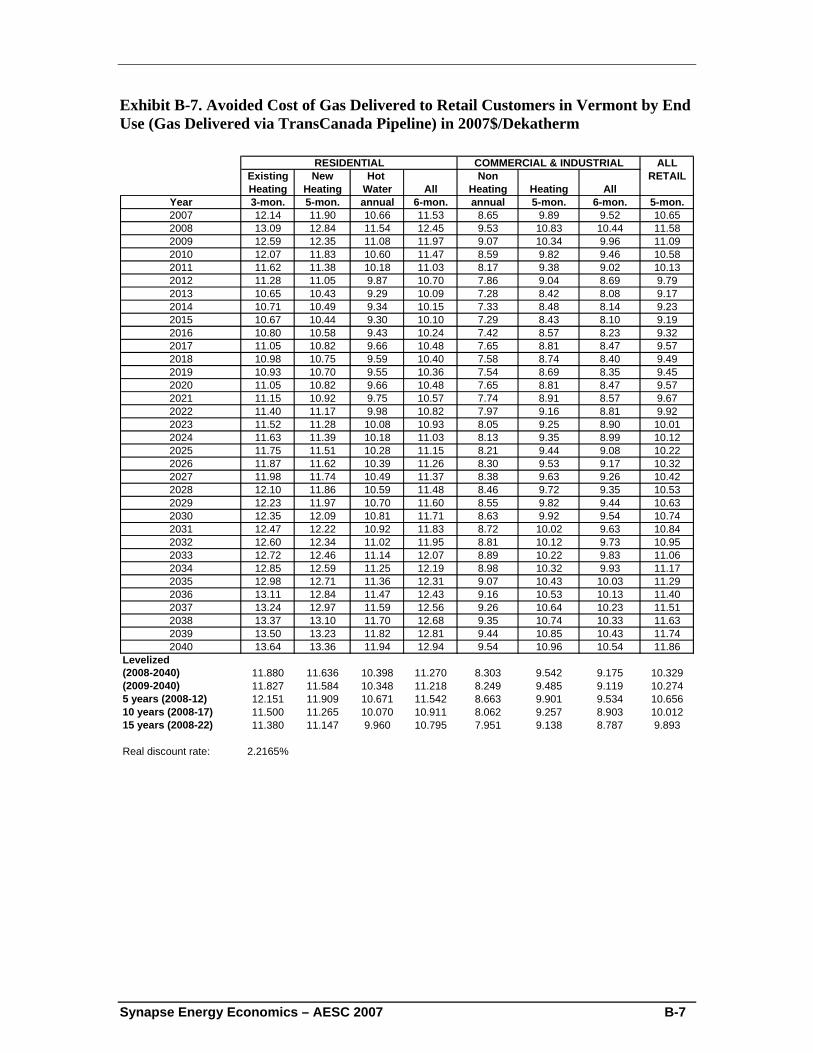
Synapse Energy Economics – AESC 2007 B-7
Exhibit B-7. Avoided Cost of Gas Delivered to Retail Customers in Vermont by End Use (Gas Delivered via TransCanada Pipeline) in 2007$/Dekatherm
ALLExisting New Hot Non RETAILHeating Heating Water All Heating Heating All
Year 3-mon. 5-mon. annual 6-mon. annual 5-mon. 6-mon. 5-mon.2007 12.14 11.90 10.66 11.53 8.65 9.89 9.52 10.652008 13.09 12.84 11.54 12.45 9.53 10.83 10.44 11.582009 12.59 12.35 11.08 11.97 9.07 10.34 9.96 11.092010 12.07 11.83 10.60 11.47 8.59 9.82 9.46 10.582011 11.62 11.38 10.18 11.03 8.17 9.38 9.02 10.132012 11.28 11.05 9.87 10.70 7.86 9.04 8.69 9.792013 10.65 10.43 9.29 10.09 7.28 8.42 8.08 9.172014 10.71 10.49 9.34 10.15 7.33 8.48 8.14 9.232015 10.67 10.44 9.30 10.10 7.29 8.43 8.10 9.192016 10.80 10.58 9.43 10.24 7.42 8.57 8.23 9.322017 11.05 10.82 9.66 10.48 7.65 8.81 8.47 9.572018 10.98 10.75 9.59 10.40 7.58 8.74 8.40 9.492019 10.93 10.70 9.55 10.36 7.54 8.69 8.35 9.452020 11.05 10.82 9.66 10.48 7.65 8.81 8.47 9.572021 11.15 10.92 9.75 10.57 7.74 8.91 8.57 9.672022 11.40 11.17 9.98 10.82 7.97 9.16 8.81 9.922023 11.52 11.28 10.08 10.93 8.05 9.25 8.90 10.012024 11.63 11.39 10.18 11.03 8.13 9.35 8.99 10.122025 11.75 11.51 10.28 11.15 8.21 9.44 9.08 10.222026 11.87 11.62 10.39 11.26 8.30 9.53 9.17 10.322027 11.98 11.74 10.49 11.37 8.38 9.63 9.26 10.422028 12.10 11.86 10.59 11.48 8.46 9.72 9.35 10.532029 12.23 11.97 10.70 11.60 8.55 9.82 9.44 10.632030 12.35 12.09 10.81 11.71 8.63 9.92 9.54 10.742031 12.47 12.22 10.92 11.83 8.72 10.02 9.63 10.842032 12.60 12.34 11.02 11.95 8.81 10.12 9.73 10.952033 12.72 12.46 11.14 12.07 8.89 10.22 9.83 11.062034 12.85 12.59 11.25 12.19 8.98 10.32 9.93 11.172035 12.98 12.71 11.36 12.31 9.07 10.43 10.03 11.292036 13.11 12.84 11.47 12.43 9.16 10.53 10.13 11.402037 13.24 12.97 11.59 12.56 9.26 10.64 10.23 11.512038 13.37 13.10 11.70 12.68 9.35 10.74 10.33 11.632039 13.50 13.23 11.82 12.81 9.44 10.85 10.43 11.742040 13.64 13.36 11.94 12.94 9.54 10.96 10.54 11.86
Levelized(2008-2040) 11.880 11.636 10.398 11.270 8.303 9.542 9.175 10.329(2009-2040) 11.827 11.584 10.348 11.218 8.249 9.485 9.119 10.2745 years (2008-12) 12.151 11.909 10.671 11.542 8.663 9.901 9.534 10.65610 years (2008-17) 11.500 11.265 10.070 10.911 8.062 9.257 8.903 10.01215 years (2008-22) 11.380 11.147 9.960 10.795 7.951 9.138 8.787 9.893
Real discount rate: 2.2165%
RESIDENTIAL COMMERCIAL & INDUSTRIAL
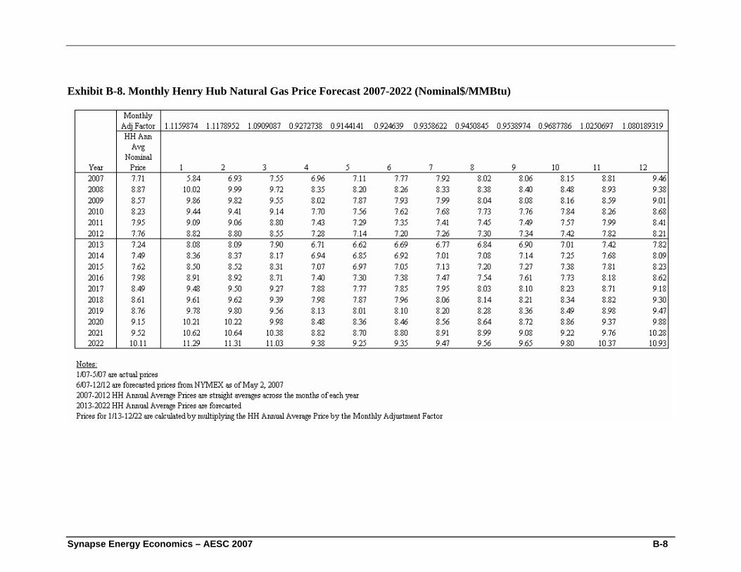
Synapse Energy Economics – AESC 2007 B-8
Exhibit B-8. Monthly Henry Hub Natural Gas Price Forecast 2007-2022 (Nominal$/MMBtu)
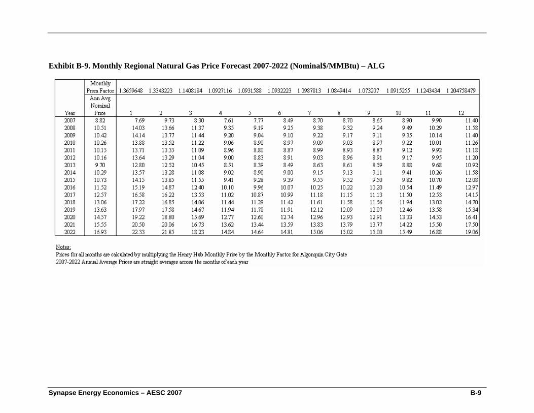
Synapse Energy Economics – AESC 2007 B-9
Exhibit B-9. Monthly Regional Natural Gas Price Forecast 2007-2022 (Nominal$/MMBtu) – ALG
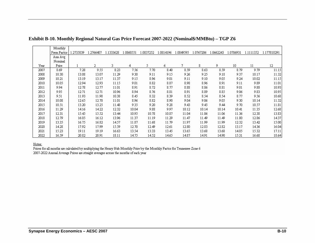
Synapse Energy Economics – AESC 2007 B-10
Exhibit B-10. Monthly Regional Natural Gas Price Forecast 2007-2022 (Nominal$/MMBtu) – TGP Z6
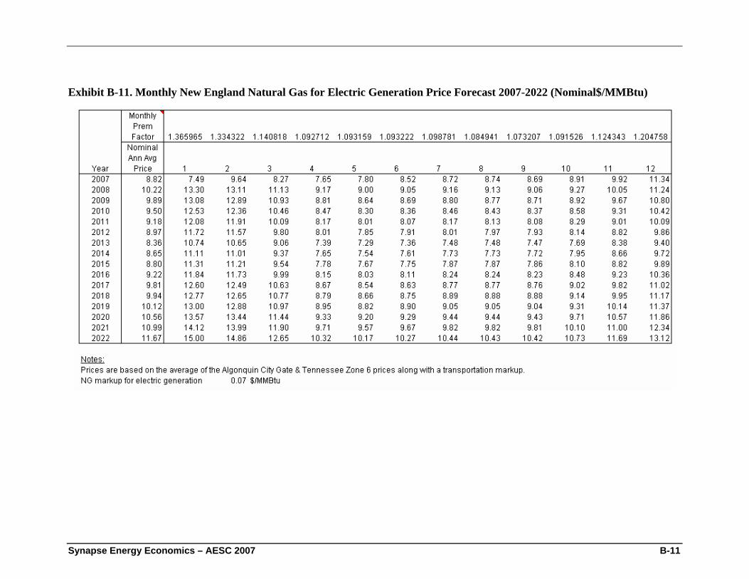
Synapse Energy Economics – AESC 2007 B-11
Exhibit B-11. Monthly New England Natural Gas for Electric Generation Price Forecast 2007-2022 (Nominal$/MMBtu)
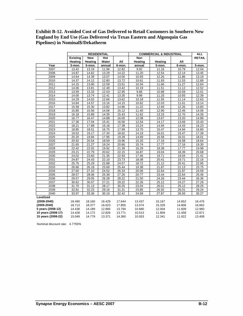
Synapse Energy Economics – AESC 2007 B-12
Exhibit B-12. Avoided Cost of Gas Delivered to Retail Customers in Southern New England by End Use (Gas Delivered via Texas Eastern and Algonquin Gas Pipelines) in Nominal$/Dekatherm
ALLExisting New Hot Non RETAILHeating Heating Water All Heating Heating All
Year 3-mon. 5-mon. annual 6-mon. annual 5-mon. 6-mon. 5-mon.2007 13.42 13.19 11.96 12.82 9.92 11.16 10.79 12.042008 14.87 14.62 13.29 14.22 11.20 12.54 12.14 13.452009 14.64 14.39 13.07 14.00 10.93 12.26 11.86 13.192010 14.37 14.12 12.80 13.72 10.61 11.93 11.53 12.892011 14.15 13.90 12.59 13.51 10.34 11.66 11.27 12.642012 14.06 13.81 12.49 13.42 10.19 11.51 11.12 12.522013 13.59 13.33 12.03 12.95 9.68 10.98 10.59 12.012014 14.00 13.74 12.41 13.35 9.99 11.33 10.93 12.392015 14.29 14.02 12.66 13.62 10.18 11.55 11.14 12.632016 14.84 14.57 13.16 14.15 10.62 12.03 11.61 13.142017 15.58 15.30 13.82 14.86 11.22 12.69 12.26 13.832018 15.85 15.56 14.06 15.12 11.40 12.90 12.45 14.062019 16.18 15.89 14.35 15.43 11.62 13.15 12.70 14.352020 16.77 16.47 14.88 16.00 12.08 13.67 13.20 14.892021 17.36 17.04 15.41 16.56 12.54 14.17 13.69 15.432022 18.21 17.88 16.18 17.38 13.24 14.94 14.43 16.232023 18.85 18.51 16.75 17.99 13.70 15.47 14.94 16.802024 19.52 19.17 17.34 18.62 14.19 16.01 15.47 17.392025 20.20 19.84 17.95 19.28 14.69 16.58 16.01 18.012026 20.92 20.54 18.59 19.96 15.20 17.16 16.58 18.642027 21.65 21.27 19.24 20.66 15.74 17.77 17.16 19.302028 22.42 22.02 19.92 21.39 16.29 18.39 17.77 19.982029 23.21 22.79 20.62 22.15 16.87 19.04 18.39 20.682030 24.02 23.60 21.35 22.93 17.46 19.71 19.04 21.412031 24.87 24.43 22.10 23.73 18.08 20.41 19.71 22.162032 25.75 25.29 22.88 24.57 18.72 21.12 20.41 22.952033 26.66 26.18 23.69 25.44 19.38 21.87 21.13 23.752034 27.60 27.10 24.52 26.33 20.06 22.64 21.87 24.592035 28.57 28.06 25.39 27.26 20.77 23.44 22.64 25.462036 29.57 29.05 26.28 28.22 21.50 24.26 23.44 26.362037 30.62 30.07 27.21 29.22 22.26 25.12 24.27 27.292038 31.70 31.13 28.17 30.25 23.04 26.01 25.12 28.252039 32.81 32.23 29.16 31.31 23.85 26.92 26.01 29.242040 33.97 33.36 30.19 32.42 24.69 27.87 26.93 30.27
Levelized (2008-2040) 18.490 18.160 16.429 17.644 13.437 15.167 14.652 16.476(2009-2040) 18.713 18.377 16.623 17.855 13.574 15.329 14.806 16.6625 years (2008-12) 14.438 14.189 12.865 13.794 10.680 12.004 11.609 12.96010 years (2008-17) 14.428 14.172 12.826 13.771 10.513 11.859 11.458 12.87115 years (2008-22) 15.049 14.779 13.371 14.360 10.933 12.341 11.922 13.408
Nominal discount rate: 4.7755%
COMMERCIAL & INDUSTRIALRESIDENTIAL
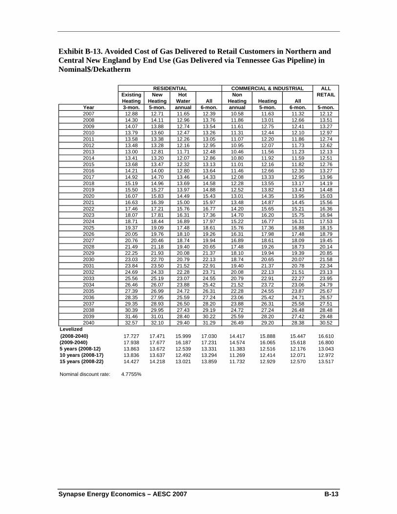
Synapse Energy Economics – AESC 2007 B-13
Exhibit B-13. Avoided Cost of Gas Delivered to Retail Customers in Northern and Central New England by End Use (Gas Delivered via Tennessee Gas Pipeline) in Nominal$/Dekatherm
ALLExisting New Hot Non RETAILHeating Heating Water All Heating Heating All
Year 3-mon. 5-mon. annual 6-mon. annual 5-mon. 6-mon. 5-mon.2007 12.88 12.71 11.65 12.39 10.58 11.63 11.32 12.122008 14.30 14.11 12.96 13.76 11.86 13.01 12.66 13.512009 14.07 13.88 12.74 13.54 11.61 12.75 12.41 13.272010 13.79 13.60 12.47 13.26 11.31 12.44 12.10 12.972011 13.58 13.38 12.26 13.05 11.07 12.20 11.86 12.742012 13.48 13.28 12.16 12.95 10.95 12.07 11.73 12.622013 13.00 12.81 11.71 12.48 10.46 11.56 11.23 12.132014 13.41 13.20 12.07 12.86 10.80 11.92 11.59 12.512015 13.68 13.47 12.32 13.13 11.01 12.16 11.82 12.762016 14.21 14.00 12.80 13.64 11.46 12.66 12.30 13.272017 14.92 14.70 13.46 14.33 12.08 13.33 12.95 13.962018 15.19 14.96 13.69 14.58 12.28 13.55 13.17 14.192019 15.50 15.27 13.97 14.88 12.52 13.82 13.43 14.482020 16.07 15.83 14.49 15.43 13.01 14.35 13.95 15.032021 16.63 16.39 15.00 15.97 13.48 14.87 14.45 15.562022 17.46 17.21 15.76 16.77 14.20 15.65 15.21 16.362023 18.07 17.81 16.31 17.36 14.70 16.20 15.75 16.942024 18.71 18.44 16.89 17.97 15.22 16.77 16.31 17.532025 19.37 19.09 17.48 18.61 15.76 17.36 16.88 18.152026 20.05 19.76 18.10 19.26 16.31 17.98 17.48 18.792027 20.76 20.46 18.74 19.94 16.89 18.61 18.09 19.452028 21.49 21.18 19.40 20.65 17.48 19.26 18.73 20.142029 22.25 21.93 20.08 21.37 18.10 19.94 19.39 20.852030 23.03 22.70 20.79 22.13 18.74 20.65 20.07 21.582031 23.84 23.50 21.52 22.91 19.40 21.37 20.78 22.342032 24.69 24.33 22.28 23.71 20.08 22.13 21.51 23.132033 25.56 25.19 23.07 24.55 20.79 22.91 22.27 23.952034 26.46 26.07 23.88 25.42 21.52 23.72 23.06 24.792035 27.39 26.99 24.72 26.31 22.28 24.55 23.87 25.672036 28.35 27.95 25.59 27.24 23.06 25.42 24.71 26.572037 29.35 28.93 26.50 28.20 23.88 26.31 25.58 27.512038 30.39 29.95 27.43 29.19 24.72 27.24 26.48 28.482039 31.46 31.01 28.40 30.22 25.59 28.20 27.42 29.482040 32.57 32.10 29.40 31.29 26.49 29.20 28.38 30.52
Levelized (2008-2040) 17.727 17.471 15.999 17.030 14.417 15.888 15.447 16.610(2009-2040) 17.938 17.677 16.187 17.231 14.574 16.065 15.618 16.8005 years (2008-12) 13.863 13.672 12.539 13.331 11.383 12.516 12.176 13.04310 years (2008-17) 13.836 13.637 12.492 13.294 11.269 12.414 12.071 12.97215 years (2008-22) 14.427 14.218 13.021 13.859 11.732 12.929 12.570 13.517
Nominal discount rate: 4.7755%
RESIDENTIAL COMMERCIAL & INDUSTRIAL
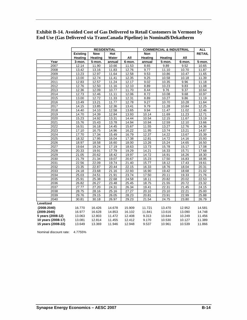
Synapse Energy Economics – AESC 2007 B-14
Exhibit B-14. Avoided Cost of Gas Delivered to Retail Customers in Vermont by End Use (Gas Delivered via TransCanada Pipeline) in Nominal$/Dekatherm
ALLExisting New Hot Non RETAILHeating Heating Water All Heating Heating All
Year 3-mon. 5-mon. annual 6-mon. annual 5-mon. 6-mon. 5-mon.2007 12.14 11.90 10.66 11.53 8.65 9.89 9.52 10.652008 13.42 13.16 11.83 12.76 9.77 11.10 10.70 11.872009 13.23 12.97 11.64 12.58 9.53 10.86 10.47 11.652010 13.00 12.74 11.41 12.35 9.25 10.58 10.18 11.392011 12.83 12.57 11.24 12.17 9.02 10.35 9.96 11.182012 12.76 12.50 11.16 12.10 8.89 10.23 9.83 11.082013 12.36 12.09 10.77 11.70 8.44 9.76 9.37 10.642014 12.73 12.46 11.11 12.06 8.72 10.08 9.68 10.972015 13.00 12.72 11.33 12.31 8.89 10.27 9.86 11.192016 13.49 13.21 11.77 12.78 9.27 10.70 10.28 11.642017 14.15 13.85 12.36 13.41 9.79 11.28 10.84 12.252018 14.40 14.10 12.58 13.65 9.94 11.47 11.02 12.462019 14.70 14.39 12.84 13.93 10.14 11.69 11.23 12.712020 15.23 14.92 13.31 14.44 10.54 12.15 11.67 13.192021 15.76 15.43 13.78 14.94 10.94 12.59 12.10 13.662022 16.51 16.18 14.45 15.67 11.55 13.27 12.76 14.362023 17.10 16.75 14.96 16.22 11.95 13.74 13.21 14.872024 17.70 17.34 15.49 16.79 12.37 14.22 13.67 15.392025 18.32 17.95 16.04 17.38 12.81 14.72 14.16 15.932026 18.97 18.58 16.60 18.00 13.26 15.24 14.65 16.502027 19.64 19.24 17.19 18.63 13.73 15.78 15.17 17.082028 20.33 19.91 17.79 19.29 14.21 16.33 15.71 17.682029 21.05 20.62 18.42 19.97 14.72 16.91 16.26 18.302030 21.79 21.34 19.07 20.67 15.23 17.50 16.83 18.952031 22.56 22.09 19.74 21.40 15.77 18.12 17.43 19.612032 23.35 22.87 20.44 22.15 16.33 18.76 18.04 20.312033 24.18 23.68 21.16 22.93 16.90 19.42 18.68 21.022034 25.03 24.51 21.91 23.74 17.50 20.11 19.33 21.762035 25.91 25.38 22.68 24.58 18.11 20.82 20.02 22.532036 26.82 26.27 23.48 25.45 18.75 21.55 20.72 23.322037 27.77 27.20 24.31 26.34 19.41 22.31 21.45 24.152038 28.75 28.16 25.16 27.27 20.10 23.10 22.21 25.002039 29.76 29.15 26.05 28.23 20.81 23.91 22.99 25.882040 30.81 30.18 26.97 29.23 21.54 24.75 23.80 26.79
Levelized (2008-2040) 16.770 16.426 14.678 15.909 11.721 13.470 12.952 14.581(2009-2040) 16.977 16.628 14.853 16.102 11.841 13.616 13.090 14.7485 years (2008-12) 13.063 12.803 11.472 12.408 9.313 10.644 10.249 11.45610 years (2008-17) 13.081 12.814 11.455 12.412 9.170 10.530 10.127 11.38915 years (2008-22) 13.649 13.369 11.946 12.948 9.537 10.961 10.539 11.866
Nominal discount rate: 4.7755%
RESIDENTIAL COMMERCIAL & INDUSTRIAL
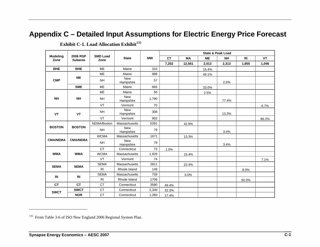
Synapse Energy Economics – AESC 2007 C-1
Appendix C – Detailed Input Assumptions for Electric Energy Price Forecast Exhibit C-1. Load Allocation Exhibit135
State & Peak Load CT MA ME NH RI VT Modeling
Zone 2006 RSP Subarea
SMD Load Zone State MW
7,252 12,561 2,013 2,313 1,855 1,046 BHE BHE ME Maine 310 15.4%
ME Maine 988 49.1% ME
NH New Hampshire 57 2.5% CMP
SME ME Maine 665 33.0% ME Maine 50 2.5%
NH New Hampshire 1,790 77.4% NH NH
VT Vermont 70 6.7%
NH New Hampshire 308 13.3% VT VT
VT Vermont 902 86.2% NEMA/Boston Massachusetts 5391 42.9%
BOSTON BOSTON NH New
Hampshire 79 3.4% WCMA Massachusetts 1671 13.3%
CMA/NEMA CMA/NEMA NH New
Hampshire 79 3.4% CT Connecticut 72 1.0%
WCMA Massachusetts 1,929 15.4% WMA WMA VT Vermont 74 7.1%
SEMA Massachusetts 2811 22.4% SEMA SEMA RI Rhode Island 149 8.0%
SEMA Massachusetts 759 6.0% RI RI RI Rhode Island 1706 92.0%
CT CT CT Connecticut 3580 49.4% SWCT CT Connecticut 2,340 32.3% SWCT NOR CT Connecticut 1,260 17.4%
135 From Table 3-6 of ISO New England 2006 Regional System Plan.
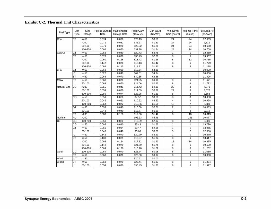
Synapse Energy Economics – AESC 2007 C-2
Exhibit C-2. Thermal Unit Characteristics
Fuel Type Unit Type
Size Range
Forced Outage Rate
Maintenance Outage Rate
Fixed O&M ($/kw-yr)
Var. O&M ($/MWh)
Min. Down Time (hours)
Min. Up Time (hours)
Full Load HR (btu/kwh)
Coal ST <=50 0.074 0.070 $79.13 $3.58 24 24 12,609>200 0.071 0.082 $31.97 $1.81 24 24 9,81150-100 0.071 0.070 $23.82 $1.28 24 24 10,650100-200 0.064 0.070 $39.78 $1.84 24 24 10,700
Gas/Oil GT <=50 0.068 0.040 $29.43 $2.75 1 1 12,459ST <=50 0.073 0.070 $30.43 $2.88 8 6 13,957
>200 0.060 0.125 $18.42 $1.26 8 12 10,73550-100 0.142 0.070 $15.13 $1.42 8 6 11,779100-200 0.065 0.115 $17.21 $1.47 8 8 11,188
LFG GT <=50 0.063 0.030 $19.54 $3.31 10,000IC <=50 0.022 0.040 $61.01 $4.34 10,036ST <=50 0.068 0.070 $30.65 $3.86 11,826
MSW ST <=50 0.068 0.070 $24.25 $0.96 8 6 11,67150-100 0.068 0.070 $24.06 $0.93 8 6 11,772
Natural Gas CC >200 0.055 0.041 $11.42 $2.19 20 8 7,07050-100 0.059 0.080 $14.69 $0.88 22 8 8,070100-200 0.059 0.074 $22.25 $1.69 8 8 8,558
CG <=50 0.059 0.080 $7.57 $0.66 8 8 10,00050-100 0.042 0.051 $10.92 $3.53 4 4 10,928100-200 0.054 0.072 $12.86 $1.58 18 7 8,689
GT <=50 0.053 0.040 $10.08 $2.01 2 1 10,86350-100 0.043 0.040 $12.77 $0.59 3 2 9,919
ST >200 0.063 0.150 $17.00 $1.42 8 10 10,313Nuclear NU >200 $92.63 $4.48 168 10,077Oil CC 100-200 0.059 0.080 $19.39 $2.12 8 8 8,000
CG <=50 0.068 0.040 $5.43 $1.62 1 1 13,726GT <=50 0.065 0.034 $9.47 $2.56 1 1 13,955
50-100 0.043 0.040 $5.66 $0.60 3 2 12,686IC <=50 0.142 0.070 $20.20 $2.21 1 1 10,370ST <=50 0.130 0.071 $13.97 $1.34 8 6 13,417
>200 0.063 0.124 $17.92 $1.43 12 14 10,38550-100 0.142 0.070 $21.80 $1.75 8 6 10,500100-200 0.069 0.120 $18.18 $1.62 8 8 11,202
Other CG 100-200 0.064 0.070 $23.74 $0.95 8 8 11,050ST <=50 0.068 0.070 $23.80 $0.97 8 6 10,000
Wind WT <=50 $20.61 $0.00Wood ST <=50 0.068 0.070 $26.44 $1.33 8 6 11,874
50-100 0.054 0.070 $30.45 $1.70 8 6 11,927
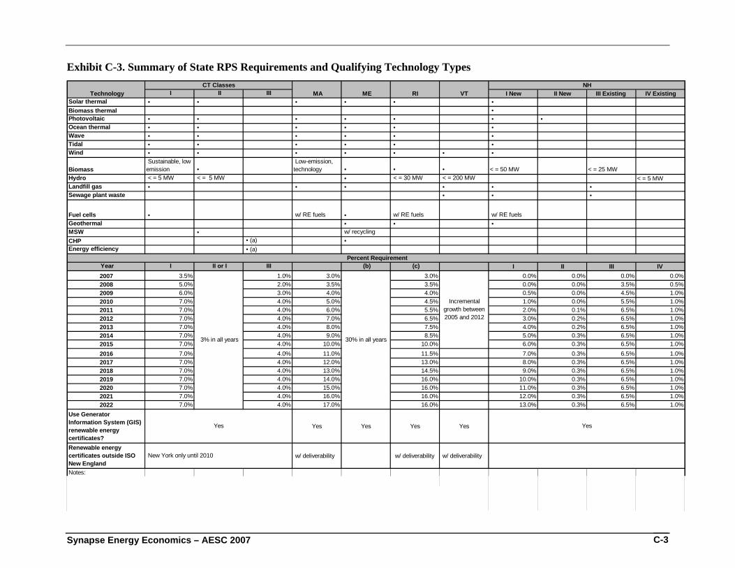
Synapse Energy Economics – AESC 2007 C-3
Exhibit C-3. Summary of State RPS Requirements and Qualifying Technology Types
I II III I New II New III Existing IV ExistingSolar thermal • • • • • • Biomass thermal • Photovoltaic • • • • • • • Ocean thermal • • • • • • Wave • • • • • • Tidal • • • • • • Wind • • • • • • •
Biomass Sustainable, low emission •
Low-emission, technology • • • < = 50 MW < = 25 MW
Hydro < = 5 MW < = 5 MW • < = 30 MW < = 200 MW < = 5 MWLandfill gas • • • • • • Sewage plant waste • • •
Fuel cells • w/ RE fuels • w/ RE fuels w/ RE fuels Geothermal • • • MSW • w/ recycling CHP • (a) • Energy efficiency • (a)
Year I II or I III (b) (c) I II III IV 2007 3.5% 1.0% 3.0% 3.0% 0.0% 0.0% 0.0% 0.0%2008 5.0% 2.0% 3.5% 3.5% 0.0% 0.0% 3.5% 0.5%2009 6.0% 3.0% 4.0% 4.0% 0.5% 0.0% 4.5% 1.0%2010 7.0% 4.0% 5.0% 4.5% 1.0% 0.0% 5.5% 1.0%2011 7.0% 4.0% 6.0% 5.5% 2.0% 0.1% 6.5% 1.0%2012 7.0% 4.0% 7.0% 6.5% 3.0% 0.2% 6.5% 1.0%2013 7.0% 4.0% 8.0% 7.5% 4.0% 0.2% 6.5% 1.0%2014 7.0% 4.0% 9.0% 8.5% 5.0% 0.3% 6.5% 1.0%2015 7.0% 4.0% 10.0% 10.0% 6.0% 0.3% 6.5% 1.0%2016 7.0% 4.0% 11.0% 11.5% 7.0% 0.3% 6.5% 1.0%2017 7.0% 4.0% 12.0% 13.0% 8.0% 0.3% 6.5% 1.0%2018 7.0% 4.0% 13.0% 14.5% 9.0% 0.3% 6.5% 1.0%2019 7.0% 4.0% 14.0% 16.0% 10.0% 0.3% 6.5% 1.0%2020 7.0% 4.0% 15.0% 16.0% 11.0% 0.3% 6.5% 1.0%2021 7.0% 4.0% 16.0% 16.0% 12.0% 0.3% 6.5% 1.0%2022 7.0% 4.0% 17.0% 16.0% 13.0% 0.3% 6.5% 1.0%
Use Generator Information System (GIS) renewable energy certificates?
Yes Yes Yes Yes
Renewable energy certificates outside ISO New England
w/ deliverability w/ deliverability w/ deliverability
Notes:
RI Technology CT Classes
MA ME
New York only until 2010
NH
Percent Requirement
Yes
30% in all years 3% in all years
Incremental growth between 2005 and 2012
Yes
VT
Synapse Energy Economics – AESC 2007 D-1
Appendix D – Usage Guide for Avoided Energy Supply Costs
A. General The avoided electricity supply cost workbook consists of a worksheet for common inputs and individual worksheets with avoided supply costs for the following geographic areas:
• Maine
• Vermont
• New Hampshire
• Connecticut (Statewide)
• Massachusetts (Statewide)
• Rhode Island
• SEMA (Southeast Massachusetts)
• WCMA (West-Central Massachusetts)
• NEMA (Northeast Massachusetts)
• Rest of Massachusetts (Massachusetts excluding NEMA)
• Norwalk/Stamford
• Southwest Connecticut, including Norwalk/Stamford
• Southwest Connecticut, excluding Norwalk/Stamford
• Rest of Connecticut (Connecticut excluding all of Southwest Connecticut)
Notifications
All present values and levelized costs in the exhibits and Avoided Cost workbook were computed using a real discount rate of 2.22%. Present values are discounted to 2007. Inflation rates of 2.9% for 2005–2006 and 2.5% for 2006–2007 were used to compare historical prices to these forecasts.
The avoided energy costs are computed for the aggregate load shape in each zone by costing period, and are applicable to DSM programs reducing load roughly in proportion to existing load. Other resources, such as load management and distributed generation, may have very different load shapes and significantly different avoided energy costs. Baseload resources, such as combined-heat-and-power (CHP) systems, would tend to
Synapse Energy Economics – AESC 2007 D-2
have lower avoided costs per kWh. Peaking resources, such as most non-CHP distributed generation and load management, would tend to have higher avoided costs per kWh.
B. Overview of Avoided Costs Each worksheet for a geographic area contains the following data for estimating the benefits of DSM.
• Avoided Energy Costs: Avoided energy costs are presented by year for four energy costing periods – Winter Peak, Winter Off-Peak, Summer Peak, and Summer Off-Peak. Avoided energy cost in each period is calculated as (relevant avoided wholesale energy cost + cost of compliance with RPS) * (1 + retail adder).
• Annual Market Capacity Value Avoided Cost: The avoided capacity cost is presented for each year stating in 2010. Avoided capacity cost in each year is calculated as (market value of capacity in the FCM assuming no new DSM increased by the required reserve margin) *(1 + retail adder) *(1 + line losses to the ISO delivery points).
• DRIPE: DRIPE energy values are presented by year for the four energy costing periods. DRIPE capacity values are presented for each year starting in 2010. It is recommended that these be included in analyses of DSM, unless specifically excluded by state or local law or regulation. It would be useful in any case to show the cost-benefit results with and without the DRIPE benefits.
• CO2 Environmental Externalities: CO2 externality values are presented by year for the four energy costing periods. It is recommended that these be included in analyses of DSM, unless specifically excluded by state or local law or regulation. It would, however, be useful in any case to show the cost-benefit results with and without the CO2 externalities included.
User-Specified Inputs
Program administrators are responsible for developing and applying losses from the ISO delivery points to the end use for their specific system when applying the avoided energy costs and avoided capacity costs.
Program Administrators have the ability to use different values for certain inputs if appropriate for a particular application. Those inputs are the retail adder, capacity factor, real discount rate, and zonal summer on-peak capacity factor. The default values for these inputs are provided in the “Inputs” worksheet. The avoided cost calculations in the worksheet for each zone use those default values via a link to the Inputs worksheet. If a user wishes to specify a different value for any of those inputs, that user-specified value should be entered directly in the relevant worksheet. This will preserve the default values in the Inputs worksheet.
Synapse Energy Economics – AESC 2007 D-3
Program administrators are responsible for developing and applying estimates of avoided transmission and distribution costs for their specific system. A suggested approach to developing those estimates is discussed below.
C. Guide to Applying the Avoided Costs The benefits of DSM should be estimated from the appropriate avoided-cost exhibit as the sum over the years of:
1. reduction in winter peak energy at the end use × winter peak energy losses from the ISO delivery points to the end use136 × the Winter Peak Energy value for that year;
2. reduction in winter off-peak energy at the end use × winter off-peak energy losses from the ISO delivery points to the end use × the Winter Off-Peak Energy value for that year;
3. reduction in summer peak energy at the end use × summer peak energy losses from the ISO delivery points to the end use × the Summer Peak Energy value for that year;
4. reduction in summer off-peak energy at the end use × summer peak off-energy losses from the ISO delivery points to the end use × the Summer Off-Peak Energy value for that year;
5. reduction in capacity costs estimated either as
a) reduction at the time of summer coincident peak at the end use × summer peak-hour losses from the ISO delivery points to the end use × the Annual Market Capacity Value for that year;
or alternatively,
b) reduction in summer peak energy at the end use × summer peak energy losses from ISO delivery to the end use × the On-Peak Summer Capacity Value for that year;
6. If the avoided costs are to include DRIPE, the avoided costs should be increased as follows:
a) If the savings persist for at least 4 years (6 years for capacity), use the values in the columns applicable to the efficiency program implementation year to calculate the sum of:
136 Each set of losses should be computed by the program administrator for its specific system.
Synapse Energy Economics – AESC 2007 D-4
i. reduction in annual winter peak energy at the end use × winter peak energy losses from ISO delivery to the end use137 × the present value line for DRIPE Winter Peak Energy;138
ii. reduction in annual winter off-peak energy at the end use × winter off-peak energy losses from ISO delivery to the end use × the present value line for DRIPE Winter Off-Peak Energy;
iii. reduction in annual summer peak energy at the end use × summer peak energy losses from ISO delivery to the end use × the present value line for DRIPE Summer Peak Energy;
iv. reduction in annual summer off-peak energy at the end use × summer off-peak energy losses from ISO delivery to the end use × the present value line for DRIPE Summer Off-Peak Energy;
v. reduction at the time of summer coincident peak at the end use × summer peak-hour losses from ISO delivery to the end use × the present value line for DRIPE Annual Market Capacity Value.
b) If savings persist for shorter periods, or if inclusion of present values is inconvenient in the benefit-cost model, DRIPE should be computed in the same manner as the direct avoided costs, as the product of load reductions and the annual DRIPE price
7. If the avoided costs are to include carbon externalities, the avoided costs should be increased as follows:139
a) reduction in winter peak energy at the end use × winter peak energy losses from the ISO delivery points to the end use × the CO2 Externality Winter Peak Energy value for that year,
b) reduction in winter off-peak energy at the end use × winter off-peak energy losses from the ISO delivery points to the end use × the CO2 Externality Winter Off-Peak Energy value for that year,
137 The loss factors relevant throughout this list should be (power at ISO delivery) ÷ (power at the end use),
and will be between 1.00 and 1.20. For some utilities, losses are reported separately as percentage losses (a) from ISO delivery to the distribution substation, and (b) from the substation to the customer; the overall loss factor can be computed as [1 + (a)] × [1 + (b)].
138 The user can change the real discount rate input to match the discount rate used in its benefit-cost model.
139 One could also make an adjustment for losses from the generator to the PTF, but that is likely more precision than is warranted by the externality value itself.
Synapse Energy Economics – AESC 2007 D-5
c) reduction in summer peak energy at the end use × summer peak energy losses from the ISO delivery points to the end use × the CO2 Externality Summer Peak Energy value for that year,
d) reduction in summer off-peak energy at the end use × summer off-peak energy losses from the ISO delivery points to the end use × the CO2 Externality Summer Off-Peak Energy value for that year,
8. If the avoided costs are to include avoided transmission and distribution costs on the program administrator’s system, the avoided costs should be increased as follows:
a) Reduction in the peak demand used in estimating avoided transmission and distribution costs at the end use × capacity losses at those peak hours from ISO delivery to the end use × the utility-specific estimate of avoided T&D costs in $/kW-year.140
D. Guide to Exhibit Structure and Terminology Each of the avoided-cost exhibits has the same structure. Reading from left to right, the structure is as follows:
i. Avoided Costs
(a) Winter Peak Energy Avoided Cost ($/kWh) 141
The 16-hour block 6am – 10pm (the hours ended 700 through 2200), Monday – Friday (except ISO holidays), in the months of January – May and October – December. Avoided energy cost in each period is calculated as (relevant avoided wholesale energy cost + cost of compliance with RPS) * (1 + retail adder).
(b) Winter Off-Peak Energy Avoided Cost ($/kWh)
All other hours – 10pm - 6am (the hours ended 2300 through 600), Monday – Friday, all day on Saturday and Sunday, and ISO holidays – in the months of January – May and October – December. Avoided energy cost in each period is calculated as (relevant avoided wholesale energy cost + cost of compliance with RPS) * (1 + retail adder).
(c) Summer Peak Energy Avoided Cost ($/kWh)
The 16-hour block 6am – 10pm (the hours ended 700 through 2200), Monday – Friday (except ISO holidays), in the months of June – September. Avoided energy cost in each
140 Most demand-response and load-management programs will not avoid transmission and distribution
costs, since they are as likely to shift local loads to new peak hours as to reduce local peaks. 141 ISO holidays are New Year’s Day, Memorial Day, July 4, Labor Day, Thanksgiving, and Christmas.
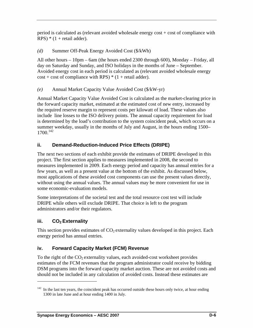
Synapse Energy Economics – AESC 2007 D-6
period is calculated as (relevant avoided wholesale energy cost + cost of compliance with RPS) * (1 + retail adder).
(d) Summer Off-Peak Energy Avoided Cost ($/kWh)
All other hours – 10pm – 6am (the hours ended 2300 through 600), Monday – Friday, all day on Saturday and Sunday, and ISO holidays in the months of June – September. Avoided energy cost in each period is calculated as (relevant avoided wholesale energy cost + cost of compliance with RPS) * (1 + retail adder).
(e) Annual Market Capacity Value Avoided Cost ($/kW-yr)
Annual Market Capacity Value Avoided Cost is calculated as the market-clearing price in the forward capacity market, estimated at the estimated cost of new entry, increased by the required reserve margin to represent costs per kilowatt of load. These values also include line losses to the ISO delivery points. The annual capacity requirement for load is determined by the load’s contribution to the system coincident peak, which occurs on a summer weekday, usually in the months of July and August, in the hours ending 1500–1700.142
ii. Demand-Reduction-Induced Price Effects (DRIPE)
The next two sections of each exhibit provide the estimates of DRIPE developed in this project. The first section applies to measures implemented in 2008, the second to measures implemented in 2009. Each energy period and capacity has annual entries for a few years, as well as a present value at the bottom of the exhibit. As discussed below, most applications of these avoided cost components can use the present values directly, without using the annual values. The annual values may be more convenient for use in some economic-evaluation models.
Some interpretations of the societal test and the total resource cost test will include DRIPE while others will exclude DRIPE. That choice is left to the program administrators and/or their regulators.
iii. CO2 Externality
This section provides estimates of CO2 externality values developed in this project. Each energy period has annual entries.
iv. Forward Capacity Market (FCM) Revenue
To the right of the CO2 externality values, each avoided-cost worksheet provides estimates of the FCM revenues that the program administrator could receive by bidding DSM programs into the forward capacity market auction. These are not avoided costs and should not be included in any calculation of avoided costs. Instead these estimates are 142 In the last ten years, the coincident peak has occurred outside these hours only twice, at hour ending
1300 in late June and at hour ending 1400 in July.
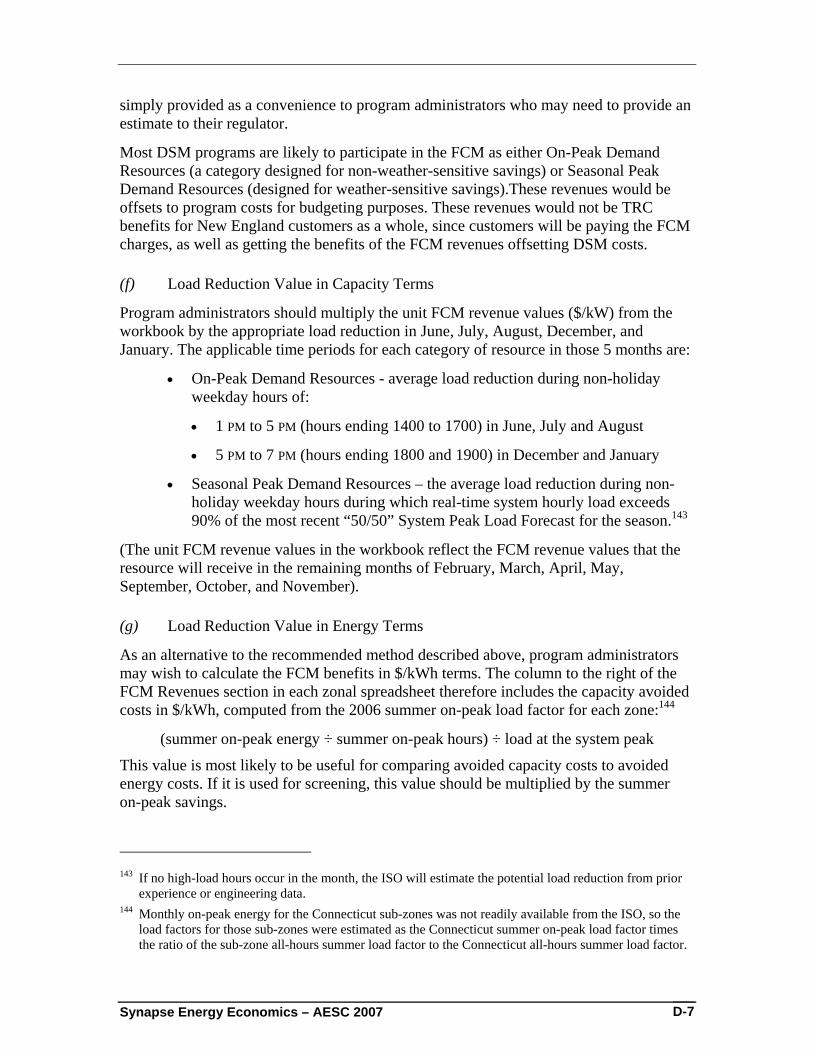
Synapse Energy Economics – AESC 2007 D-7
simply provided as a convenience to program administrators who may need to provide an estimate to their regulator.
Most DSM programs are likely to participate in the FCM as either On-Peak Demand Resources (a category designed for non-weather-sensitive savings) or Seasonal Peak Demand Resources (designed for weather-sensitive savings).These revenues would be offsets to program costs for budgeting purposes. These revenues would not be TRC benefits for New England customers as a whole, since customers will be paying the FCM charges, as well as getting the benefits of the FCM revenues offsetting DSM costs.
(f) Load Reduction Value in Capacity Terms
Program administrators should multiply the unit FCM revenue values ($/kW) from the workbook by the appropriate load reduction in June, July, August, December, and January. The applicable time periods for each category of resource in those 5 months are:
• On-Peak Demand Resources - average load reduction during non-holiday weekday hours of:
• 1 PM to 5 PM (hours ending 1400 to 1700) in June, July and August
• 5 PM to 7 PM (hours ending 1800 and 1900) in December and January
• Seasonal Peak Demand Resources – the average load reduction during non-holiday weekday hours during which real-time system hourly load exceeds 90% of the most recent “50/50” System Peak Load Forecast for the season.143
(The unit FCM revenue values in the workbook reflect the FCM revenue values that the resource will receive in the remaining months of February, March, April, May, September, October, and November).
(g) Load Reduction Value in Energy Terms
As an alternative to the recommended method described above, program administrators may wish to calculate the FCM benefits in $/kWh terms. The column to the right of the FCM Revenues section in each zonal spreadsheet therefore includes the capacity avoided costs in $/kWh, computed from the 2006 summer on-peak load factor for each zone:144
(summer on-peak energy ÷ summer on-peak hours) ÷ load at the system peak
This value is most likely to be useful for comparing avoided capacity costs to avoided energy costs. If it is used for screening, this value should be multiplied by the summer on-peak savings.
143 If no high-load hours occur in the month, the ISO will estimate the potential load reduction from prior
experience or engineering data. 144 Monthly on-peak energy for the Connecticut sub-zones was not readily available from the ISO, so the
load factors for those sub-zones were estimated as the Connecticut summer on-peak load factor times the ratio of the sub-zone all-hours summer load factor to the Connecticut all-hours summer load factor.

Synapse Energy Economics – AESC 2007 D-8
v. Input Values
To the right of the FCM values discussed above, each zonal worksheet contains the wholesale market prices and renewable-energy-credit prices applicable to that zone. These values do not reflect the addition of losses and retail adders. Users should not normally need to use these input values directly, or to modify these values.
E. Levelization Along the bottom of the tables in each zonal worksheet, there are real-levelized costs for each of the direct avoided costs. These values are calculated for various periods, using a 2.2% real discount rate and the 2.5% inflation rate assumed throughout this project. For DRIPE, whose effects are experienced over only a few years, the spreadsheet includes the present value of the energy effect per annual MWh and the capacity effect per kilowatt of load reduction, for the convenience of the program administrators. Inclusion of DRIPE would add roughly one to three years to the avoided-cost benefits.
F. Utility-Specific Costs to be Added/Considered by Program Administrators
i. Losses from the ISO Delivery Point to the End Use
The avoided energy and capacity costs, and the estimates of DRIPE, include energy and capacity losses on the ISO-administered pool transmission facilities (PTF), from the generator to the delivery points at which the PFT system connects to local non-PTF transmission or to distribution substations. The exhibits DO NOT include the following losses:
• over the non-PTF transmission substations and lines to distribution substations;
• in the distribution substations,
• from the distribution substations to the line transformers on the primary feeders and laterals,145
• from the line transformers over the secondary lines and services to the customer meter,146
• from the customer meter to the end use.
145 In some cases, this may involve multiple stages of transformers and distribution, as (for example) power
is transformed from 115kV transmission to 34kV primary distribution and then to 14 kV primary distribution and then to 4 kV primary distribution, to which the line transformer is connected.
146 Some customers receive their power from the utility at primary voltage. Since virtually all electricity is used at secondary voltages, these customers generally have line transformers on the customer side of the meter and secondary distribution within the customer facility.
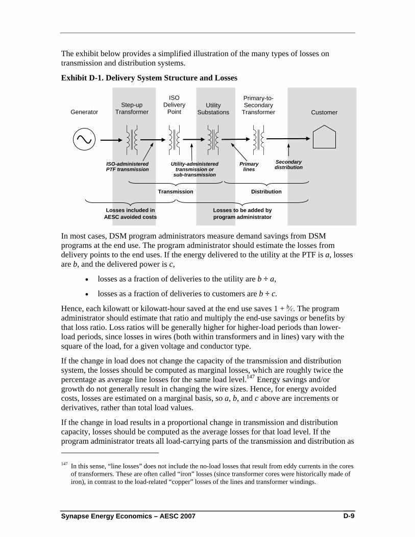
Synapse Energy Economics – AESC 2007 D-9
The exhibit below provides a simplified illustration of the many types of losses on transmission and distribution systems.
Exhibit D-1. Delivery System Structure and Losses
In most cases, DSM program administrators measure demand savings from DSM programs at the end use. The program administrator should estimate the losses from delivery points to the end uses. If the energy delivered to the utility at the PTF is a, losses are b, and the delivered power is c,
• losses as a fraction of deliveries to the utility are b ÷ a,
• losses as a fraction of deliveries to customers are b ÷ c.
Hence, each kilowatt or kilowatt-hour saved at the end use saves 1 + b⁄c. The program administrator should estimate that ratio and multiply the end-use savings or benefits by that loss ratio. Loss ratios will be generally higher for higher-load periods than lower-load periods, since losses in wires (both within transformers and in lines) vary with the square of the load, for a given voltage and conductor type.
If the change in load does not change the capacity of the transmission and distribution system, the losses should be computed as marginal losses, which are roughly twice the percentage as average line losses for the same load level.147 Energy savings and/or growth do not generally result in changing the wire sizes. Hence, for energy avoided costs, losses are estimated on a marginal basis, so a, b, and c above are increments or derivatives, rather than total load values.
If the change in load results in a proportional change in transmission and distribution capacity, losses should be computed as the average losses for that load level. If the program administrator treats all load-carrying parts of the transmission and distribution as 147 In this sense, “line losses” does not include the no-load losses that result from eddy currents in the cores
of transformers. These are often called “iron” losses (since transformer cores were historically made of iron), in contrast to the load-related “copper” losses of the lines and transformer windings.
Generator Step-up
Transformer
ISO Delivery
Point
Primary-to-Secondary
Transformer CustomerUtility
Substations
Utility-administered transmission or
sub-transmission
Primary lines
Secondary distribution
Transmission Distribution
Losses included in AESC avoided costs
Losses to be added by program administrator
ISO-administered PTF transmission
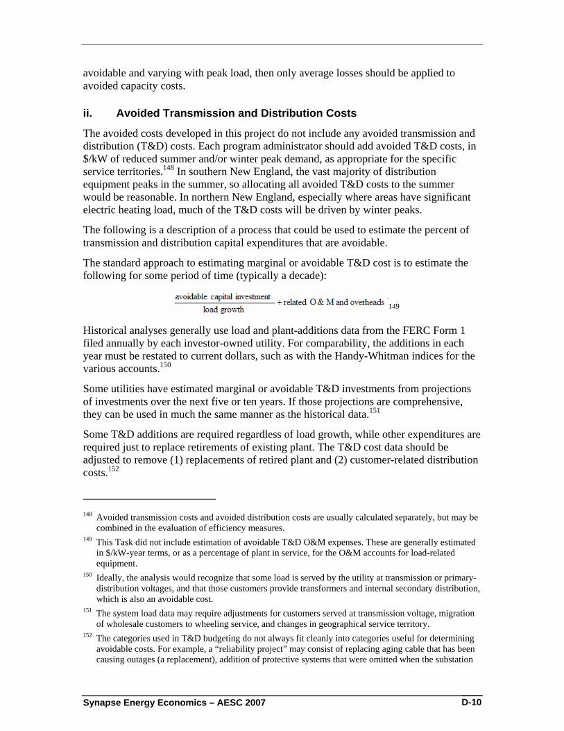
Synapse Energy Economics – AESC 2007 D-10
avoidable and varying with peak load, then only average losses should be applied to avoided capacity costs.
ii. Avoided Transmission and Distribution Costs
The avoided costs developed in this project do not include any avoided transmission and distribution (T&D) costs. Each program administrator should add avoided T&D costs, in $/kW of reduced summer and/or winter peak demand, as appropriate for the specific service territories.148 In southern New England, the vast majority of distribution equipment peaks in the summer, so allocating all avoided T&D costs to the summer would be reasonable. In northern New England, especially where areas have significant electric heating load, much of the T&D costs will be driven by winter peaks.
The following is a description of a process that could be used to estimate the percent of transmission and distribution capital expenditures that are avoidable.
The standard approach to estimating marginal or avoidable T&D cost is to estimate the following for some period of time (typically a decade):
149
Historical analyses generally use load and plant-additions data from the FERC Form 1 filed annually by each investor-owned utility. For comparability, the additions in each year must be restated to current dollars, such as with the Handy-Whitman indices for the various accounts.150
Some utilities have estimated marginal or avoidable T&D investments from projections of investments over the next five or ten years. If those projections are comprehensive, they can be used in much the same manner as the historical data.151
Some T&D additions are required regardless of load growth, while other expenditures are required just to replace retirements of existing plant. The T&D cost data should be adjusted to remove (1) replacements of retired plant and (2) customer-related distribution costs.152
148 Avoided transmission costs and avoided distribution costs are usually calculated separately, but may be
combined in the evaluation of efficiency measures. 149 This Task did not include estimation of avoidable T&D O&M expenses. These are generally estimated
in $/kW-year terms, or as a percentage of plant in service, for the O&M accounts for load-related equipment.
150 Ideally, the analysis would recognize that some load is served by the utility at transmission or primary-distribution voltages, and that those customers provide transformers and internal secondary distribution, which is also an avoidable cost.
151 The system load data may require adjustments for customers served at transmission voltage, migration of wholesale customers to wheeling service, and changes in geographical service territory.
152 The categories used in T&D budgeting do not always fit cleanly into categories useful for determining avoidable costs. For example, a “reliability project” may consist of replacing aging cable that has been causing outages (a replacement), addition of protective systems that were omitted when the substation
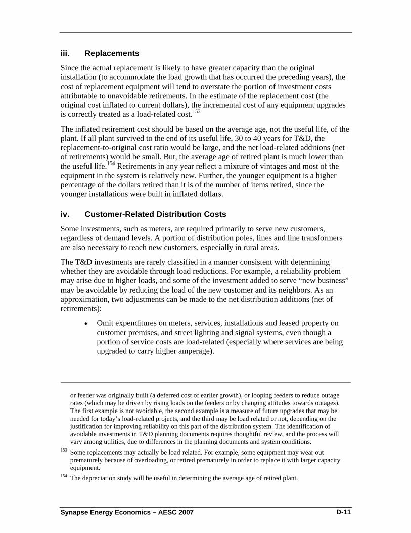
Synapse Energy Economics – AESC 2007 D-11
iii. Replacements
Since the actual replacement is likely to have greater capacity than the original installation (to accommodate the load growth that has occurred the preceding years), the cost of replacement equipment will tend to overstate the portion of investment costs attributable to unavoidable retirements. In the estimate of the replacement cost (the original cost inflated to current dollars), the incremental cost of any equipment upgrades is correctly treated as a load-related cost.153
The inflated retirement cost should be based on the average age, not the useful life, of the plant. If all plant survived to the end of its useful life, 30 to 40 years for T&D, the replacement-to-original cost ratio would be large, and the net load-related additions (net of retirements) would be small. But, the average age of retired plant is much lower than the useful life.154 Retirements in any year reflect a mixture of vintages and most of the equipment in the system is relatively new. Further, the younger equipment is a higher percentage of the dollars retired than it is of the number of items retired, since the younger installations were built in inflated dollars.
iv. Customer-Related Distribution Costs
Some investments, such as meters, are required primarily to serve new customers, regardless of demand levels. A portion of distribution poles, lines and line transformers are also necessary to reach new customers, especially in rural areas.
The T&D investments are rarely classified in a manner consistent with determining whether they are avoidable through load reductions. For example, a reliability problem may arise due to higher loads, and some of the investment added to serve “new business” may be avoidable by reducing the load of the new customer and its neighbors. As an approximation, two adjustments can be made to the net distribution additions (net of retirements):
• Omit expenditures on meters, services, installations and leased property on customer premises, and street lighting and signal systems, even though a portion of service costs are load-related (especially where services are being upgraded to carry higher amperage).
or feeder was originally built (a deferred cost of earlier growth), or looping feeders to reduce outage rates (which may be driven by rising loads on the feeders or by changing attitudes towards outages). The first example is not avoidable, the second example is a measure of future upgrades that may be needed for today’s load-related projects, and the third may be load related or not, depending on the justification for improving reliability on this part of the distribution system. The identification of avoidable investments in T&D planning documents requires thoughtful review, and the process will vary among utilities, due to differences in the planning documents and system conditions.
153 Some replacements may actually be load-related. For example, some equipment may wear out prematurely because of overloading, or retired prematurely in order to replace it with larger capacity equipment.
154 The depreciation study will be useful in determining the average age of retired plant.
Synapse Energy Economics – AESC 2007 D-12
• Reduce expenditures in all distribution accounts except substations by a percentage determined to be customer-related.
The “minimum system” method is frequently used to estimate the portion of plant that is not avoidable. It attempts to estimate the cost of the distribution system as if each unit of equipment were the minimum-sized unit that would ever be used. The demand-related portion of the investment is the increment over the cost of the minimum-sized equipment. To maintain consistency in the computation of avoidable cost per kilowatt, the loads served by that minimum-sized equipment should be removed along with the cost of that equipment.
It is likely that multiplying the cost of the minimum-sized equipment times the number of units overstates the customer-related distribution investment, since demand affects the number of transformers and the feet of conductor and conduit, as well as the size of the transformers and lines.
v. Avoidable Percent of T&D Capital
The percent of T&D capital expenditures that is avoidable would be the value estimated from the adjustment above for replacements and customer-related plant, divided by the gross expenditures. This percentage is not really needed once the adjusted investments have been estimated. An avoidable percentage estimated from one data set (e.g., historical FERC data) should not be applied to a different data set (e.g., current utility forecasts), unless the two data sets can be determined to be equally comprehensive.
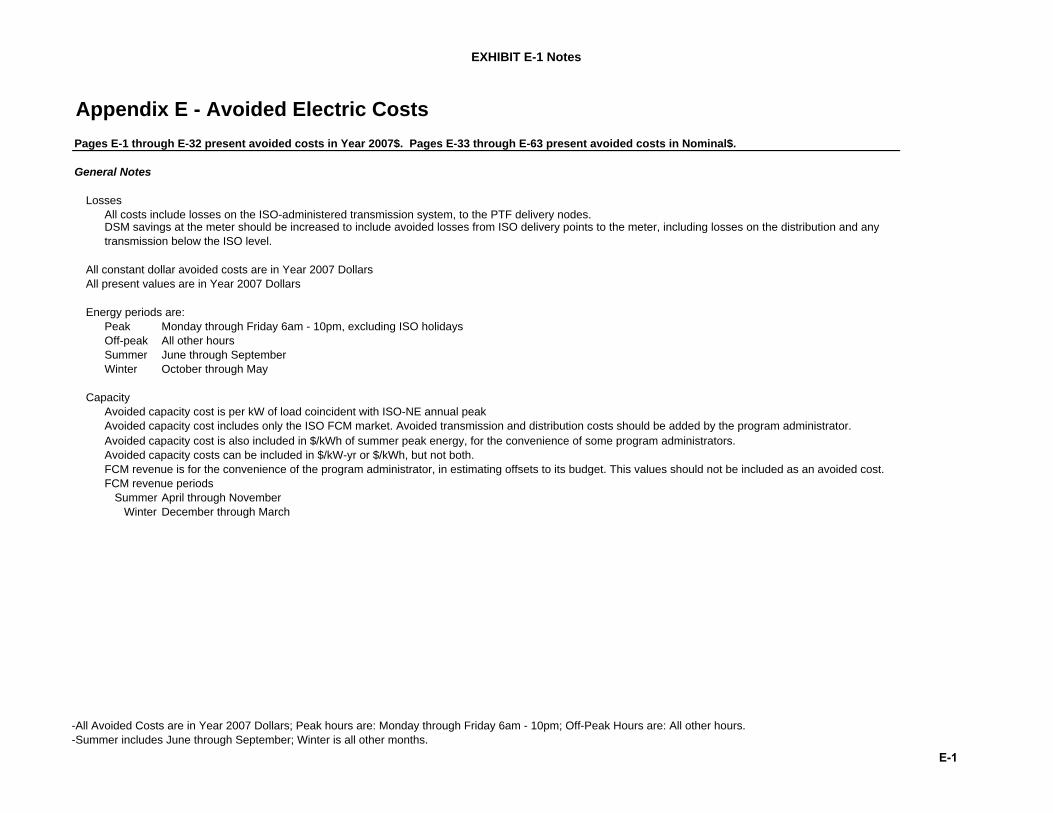
EXHIBIT E-1 Notes
Appendix E - Avoided Electric CostsPages E-1 through E-32 present avoided costs in Year 2007$. Pages E-33 through E-63 present avoided costs in Nominal$.
General Notes
LossesAll costs include losses on the ISO-administered transmission system, to the PTF delivery nodes.
All constant dollar avoided costs are in Year 2007 DollarsAll present values are in Year 2007 Dollars
Energy periods are:Peak Monday through Friday 6am - 10pm, excluding ISO holidaysOff-peak All other hoursSummer June through SeptemberWinter October through May
CapacityAvoided capacity cost is per kW of load coincident with ISO-NE annual peakAvoided capacity cost includes only the ISO FCM market. Avoided transmission and distribution costs should be added by the program administrator.
FCM revenue is for the convenience of the program administrator, in estimating offsets to its budget. This values should not be included as an avoided cost.FCM revenue periods
Summer April through NovemberWinter December through March
Avoided capacity cost is also included in $/kWh of summer peak energy, for the convenience of some program administrators. Avoided capacity costs can be included in $/kW-yr or $/kWh, but not both.
DSM savings at the meter should be increased to include avoided losses from ISO delivery points to the meter, including losses on the distribution and any transmission below the ISO level.
-All Avoided Costs are in Year 2007 Dollars; Peak hours are: Monday through Friday 6am - 10pm; Off-Peak Hours are: All other hours.-Summer includes June through September; Winter is all other months.
E-1
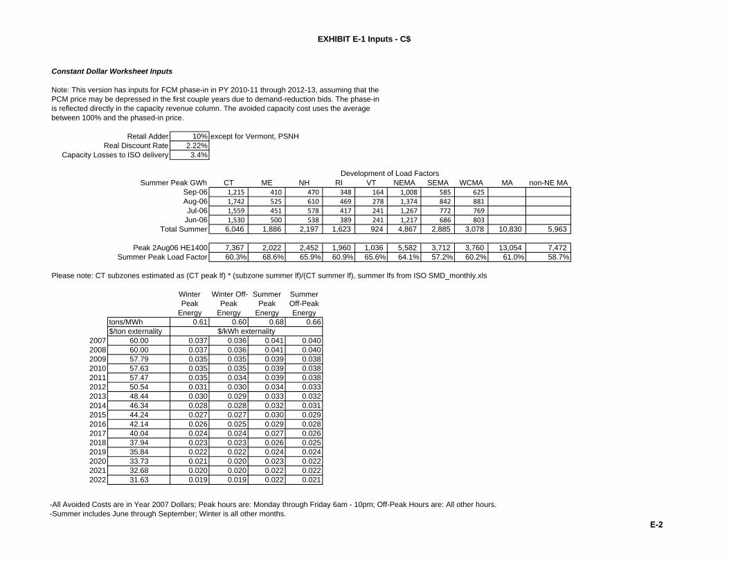
EXHIBIT E-1 Inputs - C$
Constant Dollar Worksheet Inputs
Retail Adder 10% except for Vermont, PSNHReal Discount Rate 2.22%
Capacity Losses to ISO delivery 3.4%
Summer Peak GWh CT ME NH RI VT NEMA SEMA WCMA MA non-NE MASep-06 1,215 410 470 348 164 1,008 585 625 Aug-06 1,742 525 610 469 278 1,374 842 881 Jul-06 1,559 451 578 417 241 1,267 772 769
Jun-06 1,530 500 538 389 241 1,217 686 803 Total Summer 6,046 1,886 2,197 1,623 924 4,867 2,885 3,078 10,830 5,963
Peak 2Aug06 HE1400 7,367 2,022 2,452 1,960 1,036 5,582 3,712 3,760 13,054 7,472 Summer Peak Load Factor 60.3% 68.6% 65.9% 60.9% 65.6% 64.1% 57.2% 60.2% 61.0% 58.7%
Please note: CT subzones estimated as (CT peak lf) * (subzone summer lf)/(CT summer lf), summer lfs from ISO SMD_monthly.xls
Winter Peak
Energy
Winter Off-Peak
Energy
Summer Peak
Energy
Summer Off-Peak Energy
tons/MWh 0.61 0.60 0.68 0.66$/ton externality
2007 60.00 0.037 0.036 0.041 0.0402008 60.00 0.037 0.036 0.041 0.0402009 57.79 0.035 0.035 0.039 0.0382010 57.63 0.035 0.035 0.039 0.0382011 57.47 0.035 0.034 0.039 0.0382012 50.54 0.031 0.030 0.034 0.0332013 48.44 0.030 0.029 0.033 0.0322014 46.34 0.028 0.028 0.032 0.0312015 44.24 0.027 0.027 0.030 0.0292016 42.14 0.026 0.025 0.029 0.0282017 40.04 0.024 0.024 0.027 0.0262018 37.94 0.023 0.023 0.026 0.0252019 35.84 0.022 0.022 0.024 0.0242020 33.73 0.021 0.020 0.023 0.0222021 32.68 0.020 0.020 0.022 0.0222022 31.63 0.019 0.019 0.022 0.021
Note: This version has inputs for FCM phase-in in PY 2010-11 through 2012-13, assuming that the PCM price may be depressed in the first couple years due to demand-reduction bids. The phase-in is reflected directly in the capacity revenue column. The avoided capacity cost uses the average between 100% and the phased-in price.
$/kWh externality
Development of Load Factors
-All Avoided Costs are in Year 2007 Dollars; Peak hours are: Monday through Friday 6am - 10pm; Off-Peak Hours are: All other hours.-Summer includes June through September; Winter is all other months.
E-2

EXHIBIT E-1 CT-C$
AESC Constant Dollar Avoided Cost Results by Screening ZoneNOTE: All Avoided Costs are in Year 2007 Dollars; Peak hours are: Monday through Friday 6am - 10pm; Off-Peak Hours are: All other hours Summer for energy values includes June through September; Winter is all other monthsAll Costs include losses on the ISO-administered Transmission System. DSM savings should include distribution and local transmission losses Retail Adder 10%
Real Discount Rate 2.2%Formatted for input to DSM screening models Capacity Losses: Generation to ISO Delivery 3.4%
Zonal On-Peak Summer Load Factor 60%ELECTRIC AVOIDED COSTS
Winter Peak
Energy
Winter Off-Peak
Energy
Summer Peak
Energy
Summer Off-Peak Energy
Annual Market
Capacity Value
Winter Peak
Energy
Winter Off-Peak
Energy
Summer Peak
Energy
Summer Off-Peak Energy
Annual Market
Capacity Value
Winter Peak
Energy
Winter Off-Peak
Energy
Summer Peak
Energy
Summer Off-Peak Energy
Annual Market
Capacity Value
Units: $/kWh $/kWh $/kWh $/kWh $/kW-yr $/kWh $/kWh $/kWh $/kWh $/kW-yr $/kWh $/kWh $/kWh $/kWh $/kW-yr
Period:2007 0.099 0.073 0.104 0.076 - 2008 0.111 0.083 0.106 0.081 - 0.017 0.013 0.033 0.016 - - - - - - 2009 0.104 0.079 0.107 0.073 - 0.049 0.039 0.100 0.051 - 0.017 0.013 0.033 0.016 - 2010 0.101 0.075 0.104 0.071 60.5 0.046 0.037 0.097 0.050 72 0.049 0.039 0.100 0.051 - 2011 0.097 0.071 0.103 0.069 109.1 0.028 0.023 0.059 0.030 140 0.046 0.037 0.097 0.050 - 2012 0.098 0.072 0.106 0.070 122.1 90 0.028 0.023 0.059 0.030 1402013 0.093 0.066 0.100 0.065 129.6 40 902014 0.094 0.066 0.099 0.066 129.6 402015 0.092 0.066 0.100 0.065 129.62016 0.093 0.068 0.102 0.067 129.62017 0.097 0.070 0.106 0.069 129.62018 0.095 0.070 0.104 0.069 129.62019 0.094 0.068 0.104 0.068 129.62020 0.096 0.071 0.108 0.069 129.62021 0.096 0.071 0.110 0.069 129.62022 0.100 0.072 0.113 0.071 129.62023 0.101 0.073 0.115 0.072 129.62024 0.103 0.074 0.117 0.073 129.62025 0.104 0.075 0.118 0.074 129.62026 0.106 0.076 0.120 0.075 129.62027 0.107 0.077 0.122 0.076 129.62028 0.109 0.078 0.123 0.078 129.62029 0.110 0.079 0.125 0.079 129.62030 0.112 0.080 0.127 0.080 129.62031 0.114 0.082 0.129 0.081 129.62032 0.115 0.083 0.131 0.082 129.62033 0.117 0.084 0.133 0.083 129.62034 0.119 0.085 0.135 0.085 129.62035 0.120 0.086 0.137 0.086 129.62036 0.122 0.088 0.139 0.087 129.62037 0.124 0.089 0.141 0.088 129.62038 0.126 0.090 0.143 0.090 129.62039 0.127 0.091 0.145 0.091 129.62040 0.129 0.093 0.147 0.092 129.6
Levelized(2008-2040) 0.105 0.076 0.116 0.075 114.9 0.006 0.005 0.012 0.006 13.4 0.006 0.004 0.012 0.006 10.3(2009-2040) 0.105 0.076 0.116 0.075 120.0 0.005 0.004 0.011 0.005 14.0 0.006 0.005 0.012 0.006 10.75 years (2008-12) 0.102 0.076 0.105 0.073 56.8 0.028 0.023 0.058 0.030 59.0 0.028 0.022 0.057 0.029 26.810 years (2008-17) 0.098 0.072 0.103 0.070 91.2 0.015 0.012 0.031 0.016 35.1 0.015 0.012 0.030 0.015 26.915 years (2008-22) 0.098 0.071 0.105 0.070 102.6 0.010 0.008 0.022 0.011 24.6 0.010 0.008 0.021 0.011 18.9PV to 2008 0.135 0.109 0.279 0.141 318.3 0.132 0.106 0.273 0.138 243.9PV to 2009 0.135 0.109 0.279 0.141 249.3
Notes: 1) Capacity price converted to $/kWh at zonal on-peak summer load factor.2) Projected environmental costs represent costs that are not yet internalized. Sustainability Target = Allowance Price (internalized value) + Environmental Cost
Connecticut DRIPE for Installations in 2008 DRIPE for Installations in 2009
Wholesale Power Price, Constant Dollars
-All Avoided Costs are in Year 2007 Dollars; Peak hours are: Monday through Friday 6am - 10pm; Off-Peak Hours are: All other hours.-Summer includes June through September; Winter is all other months.
E-3

EXHIBIT E-1 CT-C$
Units:
Period:2007200820092010201120122013201420152016201720182019202020212022202320242025202620272028202920302031203220332034203520362037203820392040
Levelized(2008-2040)(2009-2040)5 years (2008-12)10 years (2008-17)15 years (2008-22)PV to 2008PV to 2009
AESC Constant Dollar Avoided Cost Results by Screening ZoneNOTE: All Avoided Costs are in Year 2007 Dollars; Peak hours are: Monday through Friday 6am - 10pm; Off-Peak Hours are: All other hours Summer for energy values includes June through September; Winter is all other monthsAll Costs include losses on the ISO-administered Transmission System. DSM savings should include distribution and local transmission losses
2010-11 60%Formatted for input to DSM screening models 2011-12 80%
2012-13 100%2013-14 100%
REC Costs
Winter Peak
Energy
Winter Off-Peak
Energy
Summer Peak
Energy
Summer Off-Peak Energy
Summer: June, July,
August
Winter: December,
January
On-Peak Summer Capacity Value1
Winter Peak
Energy
Winter Off-Peak
Energy
Summer Peak
Energy
Summer Off-Peak Energy
Annual Market
Capacity Value
All Energy
$/kWh $/kWh $/kWh $/kWh $/kW-month
$/kW-month $/kWh $/kWh $/kWh $/kWh $/kWh $/kW-yr ¢/kWh $/kW-yr
0.037 0.036 0.041 0.040 0.089 0.064 0.093 0.067 0.1750.037 0.036 0.041 0.040 9.3 7.0 0.098 0.073 0.094 0.071 0.222 40.50.035 0.035 0.039 0.038 10.4 7.8 0.092 0.070 0.095 0.064 0.233 45.20.035 0.035 0.039 0.038 13.5 10.2 0.074 0.090 0.066 0.092 0.062 67 0.233 19.00.035 0.034 0.039 0.038 17.9 13.4 0.133 0.086 0.062 0.091 0.060 114 0.2110.031 0.030 0.034 0.033 23.1 17.4 0.148 0.087 0.064 0.095 0.061 114 0.1890.030 0.029 0.033 0.032 26.2 19.6 0.158 0.083 0.059 0.090 0.058 114 0.1670.028 0.028 0.032 0.031 26.2 19.6 0.158 0.084 0.059 0.089 0.059 114 0.1450.027 0.027 0.030 0.029 26.2 19.6 0.158 0.082 0.059 0.090 0.058 114 0.1230.026 0.025 0.029 0.028 26.2 19.6 0.158 0.084 0.061 0.092 0.060 114 0.0990.024 0.024 0.027 0.026 26.2 19.6 0.158 0.087 0.063 0.095 0.062 114 0.0740.023 0.023 0.026 0.025 26.2 19.6 0.158 0.086 0.063 0.094 0.063 114 0.0490.022 0.022 0.024 0.024 26.2 19.6 0.158 0.085 0.062 0.095 0.061 114 0.0250.021 0.020 0.023 0.022 26.2 19.6 0.158 0.087 0.064 0.098 0.063 114 0.0000.020 0.020 0.022 0.022 26.2 19.6 0.158 0.087 0.064 0.100 0.063 114 0.0000.019 0.019 0.022 0.021 26.2 19.6 0.158 0.091 0.065 0.103 0.065 114 0.0000.019 0.019 0.022 0.021 26.2 19.6 0.158 0.092 0.066 0.104 0.066 1140.019 0.019 0.022 0.021 26.2 19.6 0.158 0.093 0.067 0.106 0.067 1140.019 0.019 0.022 0.021 26.2 19.6 0.158 0.095 0.068 0.107 0.068 1140.019 0.019 0.022 0.021 26.2 19.6 0.158 0.096 0.069 0.109 0.069 1140.019 0.019 0.022 0.021 26.2 19.6 0.158 0.097 0.070 0.111 0.070 1140.019 0.019 0.022 0.021 26.2 19.6 0.158 0.099 0.071 0.112 0.071 1140.019 0.019 0.022 0.021 26.2 19.6 0.158 0.100 0.072 0.114 0.072 1140.019 0.019 0.022 0.021 26.2 19.6 0.158 0.102 0.073 0.115 0.073 1140.019 0.019 0.022 0.021 26.2 19.6 0.158 0.103 0.074 0.117 0.074 1140.019 0.019 0.022 0.021 26.2 19.6 0.158 0.105 0.075 0.119 0.075 1140.019 0.019 0.022 0.021 26.2 19.6 0.158 0.106 0.076 0.121 0.076 1140.019 0.019 0.022 0.021 26.2 19.6 0.158 0.108 0.077 0.122 0.077 1140.019 0.019 0.022 0.021 26.2 19.6 0.158 0.109 0.079 0.124 0.078 1140.019 0.019 0.022 0.021 26.2 19.6 0.158 0.111 0.080 0.126 0.079 1140.019 0.019 0.022 0.021 26.2 19.6 0.158 0.113 0.081 0.128 0.080 1140.019 0.019 0.022 0.021 26.2 19.6 0.158 0.114 0.082 0.130 0.081 1140.019 0.019 0.022 0.021 26.2 19.6 0.158 0.116 0.083 0.131 0.083 1140.019 0.019 0.022 0.021 26.2 19.6 0.158 0.117 0.084 0.133 0.084 114
0.024 0.024 0.027 0.026 23.9 17.9 0.1370.024 0.023 0.026 0.025 24.5 18.4 0.1400.035 0.034 0.039 0.037 14.7 11.0 0.0150.031 0.031 0.035 0.034 20.1 15.1 0.0860.028 0.028 0.031 0.030 21.9 16.4 0.111
Notes: 1) Capacity price converted to $/kWh at zonal on-peak summer load factor.2) Projected environmental costs represent costs that are not yet internalized. Sustainability Target = Allowance Price (internalized value) + Environmental Cost
Wholesale Power Price, Constant Dollars FCM Revenue
(not an avoided cost; do not add to avoided costs) Avoided Costs before Adders
FCM phase-in
Additional CO2 Costs(see note below)
ICAP
-All Avoided Costs are in Year 2007 Dollars; Peak hours are: Monday through Friday 6am - 10pm; Off-Peak Hours are: All other hours.-Summer includes June through September; Winter is all other months.
E-4

EXHIBIT E-1 ME-C$
AESC Constant Dollar Avoided Cost Results by Screening ZoneNOTE: All Avoided Costs are in Year 2007 Dollars; Peak hours are: Monday through Friday 6am - 10pm; Off-Peak Hours are: All other hours Summer for energy values includes June through September; Winter is all other monthsAll Costs include losses on the ISO-administered Transmission System. DSM savings should include distribution and local transmission losses Retail Adder 10%
Real Discount Rate 2.2%Formatted for input to DSM screening models Capacity Losses: Generation to ISO Delivery 3.4%
Zonal On-Peak Summer Load Factor 69%ELECTRIC AVOIDED COSTS
Winter Peak
Energy
Winter Off-Peak
Energy
Summer Peak
Energy
Summer Off-Peak Energy
Annual Market
Capacity Value
Winter Peak
Energy
Winter Off-Peak
Energy
Summer Peak
Energy
Summer Off-Peak Energy
Annual Market
Capacity Value
Winter Peak
Energy
Winter Off-Peak
Energy
Summer Peak
Energy
Summer Off-Peak Energy
Annual Market
Capacity Value
Units: $/kWh $/kWh $/kWh $/kWh $/kW-yr $/kWh $/kWh $/kWh $/kWh $/kW-yr $/kWh $/kWh $/kWh $/kWh $/kW-yr
Period:2007 0.082 0.061 0.082 0.063 0.0002008 0.092 0.070 0.087 0.066 0.000 0.015 0.012 0.024 0.010 - - - - - - 2009 0.089 0.068 0.083 0.063 0.000 0.044 0.037 0.069 0.030 - 0.015 0.012 0.024 0.010 - 2010 0.085 0.063 0.082 0.060 60.5 0.041 0.034 0.065 0.028 72 0.044 0.037 0.069 0.030 - 2011 0.081 0.061 0.081 0.058 109.1 0.025 0.020 0.040 0.017 140 0.041 0.034 0.065 0.028 - 2012 0.083 0.062 0.085 0.060 122.1 90 0.025 0.020 0.040 0.017 1402013 0.079 0.058 0.081 0.057 129.6 40 902014 0.082 0.059 0.083 0.058 125.400 402015 0.081 0.059 0.084 0.057 125.4002016 0.083 0.060 0.087 0.060 125.4002017 0.085 0.062 0.089 0.060 125.4002018 0.082 0.062 0.087 0.060 125.4002019 0.083 0.060 0.091 0.060 125.4002020 0.084 0.061 0.091 0.060 125.4002021 0.085 0.063 0.093 0.061 125.4002022 0.087 0.064 0.097 0.062 125.4002023 0.088 0.065 0.098 0.062 125.4002024 0.090 0.066 0.100 0.063 125.4002025 0.091 0.067 0.101 0.064 125.4002026 0.092 0.068 0.102 0.065 125.4002027 0.094 0.069 0.104 0.066 125.4002028 0.095 0.070 0.105 0.067 125.4002029 0.096 0.071 0.107 0.068 125.4002030 0.098 0.072 0.109 0.069 125.4002031 0.099 0.073 0.110 0.070 125.4002032 0.101 0.074 0.112 0.071 125.4002033 0.102 0.075 0.113 0.072 125.4002034 0.104 0.076 0.115 0.073 125.4002035 0.105 0.077 0.117 0.074 125.4002036 0.107 0.078 0.118 0.075 125.4002037 0.108 0.079 0.120 0.076 125.4002038 0.110 0.080 0.122 0.077 125.4002039 0.111 0.081 0.124 0.079 125.4002040 0.113 0.083 0.125 0.080 125.400
Levelized(2008-2040) 0.091 0.067 0.097 0.065 111.7 0.004 0.003 0.006 0.003 10.4 0.005 0.004 0.008 0.003 10.3(2009-2040) 0.091 0.067 0.098 0.065 116.6 0.003 0.003 0.005 0.002 10.7 0.005 0.004 0.008 0.003 10.75 years (2008-12) 0.086 0.065 0.084 0.061 56.8 0.025 0.021 0.040 0.017 60.4 0.025 0.020 0.039 0.017 26.810 years (2008-17) 0.084 0.063 0.084 0.060 89.6 0.012 0.010 0.020 0.008 34.2 0.013 0.011 0.021 0.009 26.915 years (2008-22) 0.084 0.062 0.086 0.060 100.3 0.008 0.007 0.013 0.006 22.8 0.009 0.008 0.014 0.006 18.9PV to 2008 0.120 0.099 0.191 0.081 318.3 0.118 0.097 0.187 0.080 243.9PV to 2009 0.120 0.099 0.191 0.081 249.3
Notes: 1) Capacity price converted to $/kWh at zonal on-peak summer load factor.2) Projected environmental costs represent costs that are not yet internalized. Sustainability Target = Allowance Price (internalized value) + Environmental Cost
Wholesale Power Price, Constant Dollars
Maine DRIPE for Installations in 2008 DRIPE for Installations in 2009
-All Avoided Costs are in Year 2007 Dollars; Peak hours are: Monday through Friday 6am - 10pm; Off-Peak Hours are: All other hours.-Summer includes June through September; Winter is all other months.
E-5

EXHIBIT E-1 ME-C$
Units:
Period:2007200820092010201120122013201420152016201720182019202020212022202320242025202620272028202920302031203220332034203520362037203820392040
Levelized(2008-2040)(2009-2040)5 years (2008-12)10 years (2008-17)15 years (2008-22)PV to 2008PV to 2009
AESC Constant Dollar Avoided Cost Results by Screening ZoneNOTE: All Avoided Costs are in Year 2007 Dollars; Peak hours are: Monday through Friday 6am - 10pm; Off-Peak Hours are: All other hours Summer for energy values includes June through September; Winter is all other monthsAll Costs include losses on the ISO-administered Transmission System. DSM savings should include distribution and local transmission losses
2010-11 60%Formatted for input to DSM screening models 2011-12 80%
2012-13 100%2013-14 100%
REC Costs
Winter Peak
Energy
Winter Off-Peak
Energy
Summer Peak
Energy
Summer Off-Peak Energy
Summer: June, July,
August
Winter: December,
January
On-Peak Summer Capacity Value1
Winter Peak
Energy
Winter Off-Peak
Energy
Summer Peak
Energy
Summer Off-Peak Energy
Annual Market
Capacity Value
All Energy
$/kWh $/kWh $/kWh $/kWh $/kW-month
$/kW-month $/kWh $/kWh $/kWh $/kWh $/kWh $/kW-yr ¢/kWh $/kW-yr
0.037 0.036 0.041 0.040 0.075 0.056 0.074 0.058 0.0000.037 0.036 0.041 0.040 9.3 7.0 0.083 0.064 0.078 0.060 0.044 40.50.035 0.035 0.039 0.038 10.4 7.8 0.080 0.061 0.075 0.057 0.078 45.20.035 0.035 0.039 0.038 13.5 10.2 0.065 0.076 0.057 0.074 0.053 67 0.100 19.00.035 0.034 0.039 0.038 17.9 13.4 0.117 0.073 0.055 0.072 0.051 114 0.1210.031 0.030 0.034 0.033 23.1 17.4 0.131 0.074 0.055 0.076 0.053 114 0.1350.030 0.029 0.033 0.032 26.2 19.6 0.139 0.070 0.051 0.072 0.050 114 0.1430.028 0.028 0.032 0.031 26.2 19.6 0.134 0.073 0.052 0.074 0.052 114 0.1450.027 0.027 0.030 0.029 26.2 19.6 0.134 0.072 0.052 0.075 0.050 114 0.1410.026 0.025 0.029 0.028 26.2 19.6 0.134 0.074 0.053 0.077 0.053 114 0.1270.024 0.024 0.027 0.026 26.2 19.6 0.134 0.076 0.056 0.080 0.054 114 0.1060.023 0.023 0.026 0.025 26.2 19.6 0.134 0.074 0.055 0.079 0.054 114 0.0710.022 0.022 0.024 0.024 26.2 19.6 0.134 0.075 0.054 0.082 0.054 114 0.0350.021 0.020 0.023 0.022 26.2 19.6 0.134 0.076 0.056 0.082 0.055 114 0.0000.020 0.020 0.022 0.022 26.2 19.6 0.134 0.078 0.057 0.085 0.055 114 0.0000.019 0.019 0.022 0.021 26.2 19.6 0.134 0.079 0.058 0.088 0.056 114 0.0000.019 0.019 0.022 0.021 26.2 19.6 0.134 0.080 0.059 0.089 0.057 1140.019 0.019 0.022 0.021 26.2 19.6 0.134 0.081 0.060 0.090 0.058 1140.019 0.019 0.022 0.021 26.2 19.6 0.134 0.083 0.061 0.092 0.058 1140.019 0.019 0.022 0.021 26.2 19.6 0.134 0.084 0.061 0.093 0.059 1140.019 0.019 0.022 0.021 26.2 19.6 0.134 0.085 0.062 0.094 0.060 1140.019 0.019 0.022 0.021 26.2 19.6 0.134 0.086 0.063 0.096 0.061 1140.019 0.019 0.022 0.021 26.2 19.6 0.134 0.088 0.064 0.097 0.062 1140.019 0.019 0.022 0.021 26.2 19.6 0.134 0.089 0.065 0.099 0.063 1140.019 0.019 0.022 0.021 26.2 19.6 0.134 0.090 0.066 0.100 0.064 1140.019 0.019 0.022 0.021 26.2 19.6 0.134 0.091 0.067 0.102 0.065 1140.019 0.019 0.022 0.021 26.2 19.6 0.134 0.093 0.068 0.103 0.066 1140.019 0.019 0.022 0.021 26.2 19.6 0.134 0.094 0.069 0.104 0.067 1140.019 0.019 0.022 0.021 26.2 19.6 0.134 0.095 0.070 0.106 0.067 1140.019 0.019 0.022 0.021 26.2 19.6 0.134 0.097 0.071 0.108 0.068 1140.019 0.019 0.022 0.021 26.2 19.6 0.134 0.098 0.072 0.109 0.069 1140.019 0.019 0.022 0.021 26.2 19.6 0.134 0.100 0.073 0.111 0.070 1140.019 0.019 0.022 0.021 26.2 19.6 0.134 0.101 0.074 0.112 0.071 1140.019 0.019 0.022 0.021 26.2 19.6 0.134 0.103 0.075 0.114 0.073 114
0.023 0.023 0.026 0.025 24.5 18.4 0.1180.023 0.022 0.025 0.024 24.9 18.7 0.1200.035 0.034 0.039 0.037 14.8 11.1 0.0130.031 0.030 0.034 0.033 20.5 15.4 0.0740.028 0.027 0.031 0.030 22.4 16.8 0.096
Notes: 1) Capacity price converted to $/kWh at zonal on-peak summer load factor.2) Projected environmental costs represent costs that are not yet internalized. Sustainability Target = Allowance Price (internalized value) + Environmental Cost
ICAP
Wholesale Power Price, Constant Dollars
FCM phase-in
FCM Revenue(not an avoided cost;
do not add to avoided costs) Avoided Costs before AddersAdditional CO2 Costs
(see note below)
-All Avoided Costs are in Year 2007 Dollars; Peak hours are: Monday through Friday 6am - 10pm; Off-Peak Hours are: All other hours.-Summer includes June through September; Winter is all other months.
E-6

EXHIBIT E-1 MA-C$
AESC Constant Dollar Avoided Cost Results by Screening ZoneNOTE: All Avoided Costs are in Year 2007 Dollars; Peak hours are: Monday through Friday 6am - 10pm; Off-Peak Hours are: All other hours Summer for energy values includes June through September; Winter is all other monthsAll Costs include losses on the ISO-administered Transmission System. DSM savings should include distribution and local transmission losses Retail Adder 10%
Real Discount Rate 2.2%Formatted for input to DSM screening models Capacity Losses: Generation to ISO Delivery 3.4%
Zonal On-Peak Summer Load Factor 61%ELECTRIC AVOIDED COSTS
Winter Peak
Energy
Winter Off-Peak
Energy
Summer Peak
Energy
Summer Off-Peak Energy
Annual Market
Capacity Value
Winter Peak
Energy
Winter Off-Peak
Energy
Summer Peak
Energy
Summer Off-Peak Energy
Annual Market
Capacity Value
Winter Peak
Energy
Winter Off-Peak
Energy
Summer Peak
Energy
Summer Off-Peak Energy
Annual Market
Capacity Value
Units: $/kWh $/kWh $/kWh $/kWh $/kW-yr $/kWh $/kWh $/kWh $/kWh $/kW-yr $/kWh $/kWh $/kWh $/kWh $/kW-yr
Period:2007 0.094 0.069 0.095 0.072 - 2008 0.105 0.078 0.097 0.074 - 0.016 0.013 0.029 0.012 - - - - - - 2009 0.098 0.075 0.097 0.070 - 0.046 0.037 0.083 0.034 - 0.016 0.013 0.029 0.012 - 2010 0.097 0.072 0.098 0.067 60.5 0.043 0.035 0.078 0.031 72 0.046 0.037 0.083 0.034 - 2011 0.093 0.068 0.097 0.065 109.1 0.026 0.021 0.047 0.019 140 0.043 0.035 0.078 0.031 - 2012 0.094 0.070 0.098 0.068 122.1 90 0.026 0.021 0.047 0.019 1402013 0.089 0.065 0.094 0.064 129.6 40 902014 0.091 0.065 0.094 0.065 129.6 402015 0.090 0.065 0.098 0.065 129.62016 0.092 0.066 0.099 0.068 129.62017 0.094 0.068 0.102 0.067 129.62018 0.092 0.068 0.100 0.068 129.62019 0.092 0.066 0.102 0.067 129.62020 0.093 0.068 0.103 0.067 129.62021 0.094 0.068 0.108 0.068 129.62022 0.097 0.070 0.109 0.069 129.62023 0.098 0.071 0.111 0.070 129.62024 0.100 0.072 0.113 0.071 129.62025 0.101 0.073 0.114 0.072 129.62026 0.103 0.074 0.116 0.073 129.62027 0.104 0.075 0.117 0.074 129.62028 0.106 0.076 0.119 0.075 129.62029 0.107 0.077 0.121 0.077 129.62030 0.109 0.078 0.123 0.078 129.62031 0.110 0.079 0.124 0.079 129.62032 0.112 0.080 0.126 0.080 129.62033 0.114 0.081 0.128 0.081 129.62034 0.115 0.083 0.130 0.082 129.62035 0.117 0.084 0.132 0.083 129.62036 0.119 0.085 0.134 0.085 129.62037 0.120 0.086 0.136 0.086 129.62038 0.122 0.088 0.138 0.087 129.62039 0.124 0.089 0.140 0.088 129.62040 0.126 0.090 0.142 0.090 129.6
Levelized(2008-2040) 0.102 0.074 0.111 0.073 114.9 0.005 0.004 0.010 0.004 13.4 0.005 0.004 0.009 0.004 10.3(2009-2040) 0.102 0.074 0.112 0.073 120.0 0.005 0.004 0.009 0.004 14.0 0.005 0.004 0.010 0.004 10.75 years (2008-12) 0.098 0.073 0.098 0.069 56.8 0.026 0.021 0.048 0.019 59.0 0.026 0.021 0.047 0.019 26.810 years (2008-17) 0.095 0.070 0.098 0.068 91.2 0.014 0.011 0.025 0.010 35.1 0.014 0.011 0.025 0.010 26.915 years (2008-22) 0.094 0.069 0.100 0.068 102.6 0.010 0.008 0.018 0.007 24.6 0.010 0.008 0.017 0.007 18.9PV to 2008 0.127 0.102 0.229 0.093 318.3 0.124 0.100 0.224 0.091 243.9PV to 2009 0.127 0.102 0.229 0.093 249.3
Notes: 1) Capacity price converted to $/kWh at zonal on-peak summer load factor.2) Projected environmental costs represent costs that are not yet internalized. Sustainability Target = Allowance Price (internalized value) + Environmental Cost
Wholesale Power Price, Constant Dollars
All of Massachusetts DRIPE for Installations in 2008 DRIPE for Installations in 2009
-All Avoided Costs are in Year 2007 Dollars; Peak hours are: Monday through Friday 6am - 10pm; Off-Peak Hours are: All other hours.-Summer includes June through September; Winter is all other months.
E-7
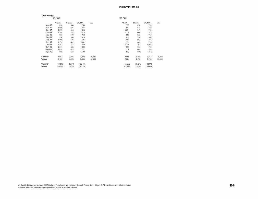
EXHIBIT E-1 MA-C$
Zonal EnergyOn-Peak Off-Peak
NEMA SEMA WCMA MA NEMA SEMA WCMA MAMar-07 890 560 750 777 478 704 Feb-07 1,049 597 635 942 533 679 Jan-07 1,253 620 823 1,074 517 769 Dec-06 1,149 574 718 1,129 609 815 Nov-06 963 579 750 851 532 713 Oct-06 994 598 579 835 514 640 Sep-06 1,008 585 625 951 562 785 Aug-06 1,374 842 881 993 609 789 Jul-06 1,267 772 769 1,235 791 1,005
Jun-06 1,217 686 803 891 524 738 May-06 1,019 623 771 779 469 686 Apr-06 866 527 670 837 518 757
Summer 4,867 2,885 3,078 10,830 4,069 2,485 3,317 9,872 Winter 8,183 4,678 5,695 18,556 7,224 4,170 5,764 17,159
Summer 44.9% 26.6% 28.4% 41.2% 25.2% 33.6%Winter 44.1% 25.2% 30.7% 42.1% 24.3% 33.6%
-All Avoided Costs are in Year 2007 Dollars; Peak hours are: Monday through Friday 6am - 10pm; Off-Peak Hours are: All other hours.-Summer includes June through September; Winter is all other months.
E-8
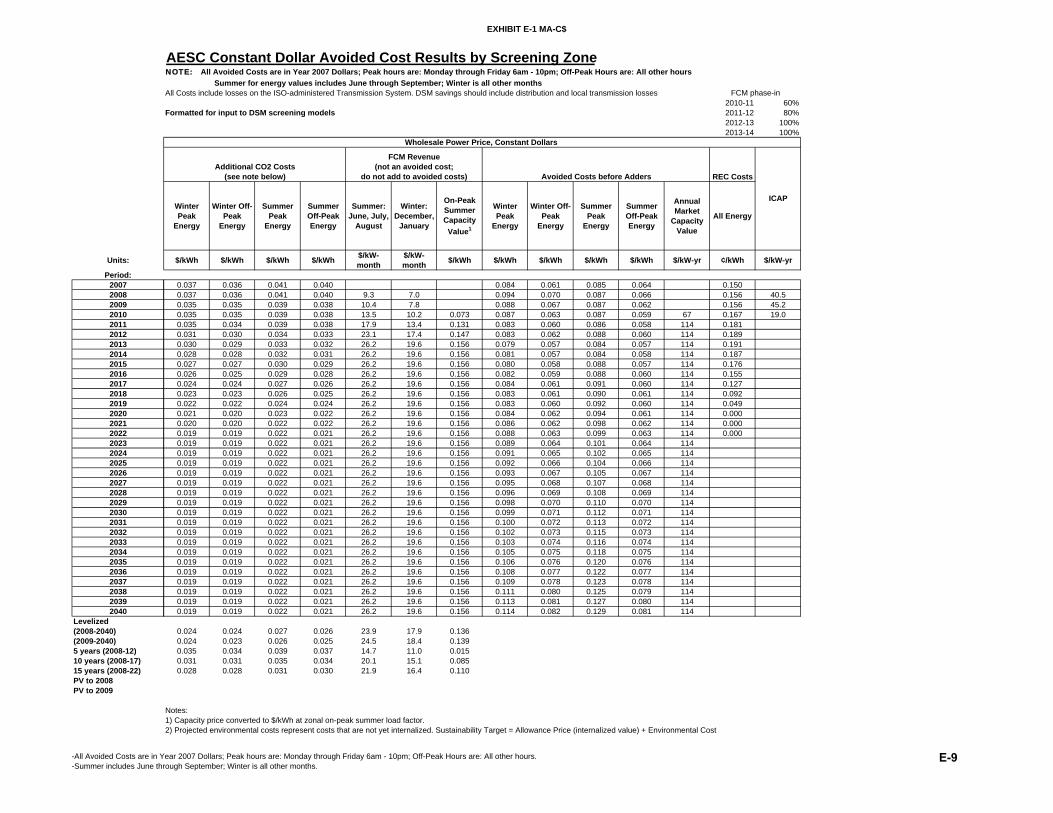
EXHIBIT E-1 MA-C$
Units:
Period:2007200820092010201120122013201420152016201720182019202020212022202320242025202620272028202920302031203220332034203520362037203820392040
Levelized(2008-2040)(2009-2040)5 years (2008-12)10 years (2008-17)15 years (2008-22)PV to 2008PV to 2009
AESC Constant Dollar Avoided Cost Results by Screening ZoneNOTE: All Avoided Costs are in Year 2007 Dollars; Peak hours are: Monday through Friday 6am - 10pm; Off-Peak Hours are: All other hours Summer for energy values includes June through September; Winter is all other monthsAll Costs include losses on the ISO-administered Transmission System. DSM savings should include distribution and local transmission losses
2010-11 60%Formatted for input to DSM screening models 2011-12 80%
2012-13 100%2013-14 100%
REC Costs
Winter Peak
Energy
Winter Off-Peak
Energy
Summer Peak
Energy
Summer Off-Peak Energy
Summer: June, July,
August
Winter: December,
January
On-Peak Summer Capacity Value1
Winter Peak
Energy
Winter Off-Peak
Energy
Summer Peak
Energy
Summer Off-Peak Energy
Annual Market
Capacity Value
All Energy
$/kWh $/kWh $/kWh $/kWh $/kW-month
$/kW-month $/kWh $/kWh $/kWh $/kWh $/kWh $/kW-yr ¢/kWh $/kW-yr
0.037 0.036 0.041 0.040 0.084 0.061 0.085 0.064 0.1500.037 0.036 0.041 0.040 9.3 7.0 0.094 0.070 0.087 0.066 0.156 40.50.035 0.035 0.039 0.038 10.4 7.8 0.088 0.067 0.087 0.062 0.156 45.20.035 0.035 0.039 0.038 13.5 10.2 0.073 0.087 0.063 0.087 0.059 67 0.167 19.00.035 0.034 0.039 0.038 17.9 13.4 0.131 0.083 0.060 0.086 0.058 114 0.1810.031 0.030 0.034 0.033 23.1 17.4 0.147 0.083 0.062 0.088 0.060 114 0.1890.030 0.029 0.033 0.032 26.2 19.6 0.156 0.079 0.057 0.084 0.057 114 0.1910.028 0.028 0.032 0.031 26.2 19.6 0.156 0.081 0.057 0.084 0.058 114 0.1870.027 0.027 0.030 0.029 26.2 19.6 0.156 0.080 0.058 0.088 0.057 114 0.1760.026 0.025 0.029 0.028 26.2 19.6 0.156 0.082 0.059 0.088 0.060 114 0.1550.024 0.024 0.027 0.026 26.2 19.6 0.156 0.084 0.061 0.091 0.060 114 0.1270.023 0.023 0.026 0.025 26.2 19.6 0.156 0.083 0.061 0.090 0.061 114 0.0920.022 0.022 0.024 0.024 26.2 19.6 0.156 0.083 0.060 0.092 0.060 114 0.0490.021 0.020 0.023 0.022 26.2 19.6 0.156 0.084 0.062 0.094 0.061 114 0.0000.020 0.020 0.022 0.022 26.2 19.6 0.156 0.086 0.062 0.098 0.062 114 0.0000.019 0.019 0.022 0.021 26.2 19.6 0.156 0.088 0.063 0.099 0.063 114 0.0000.019 0.019 0.022 0.021 26.2 19.6 0.156 0.089 0.064 0.101 0.064 1140.019 0.019 0.022 0.021 26.2 19.6 0.156 0.091 0.065 0.102 0.065 1140.019 0.019 0.022 0.021 26.2 19.6 0.156 0.092 0.066 0.104 0.066 1140.019 0.019 0.022 0.021 26.2 19.6 0.156 0.093 0.067 0.105 0.067 1140.019 0.019 0.022 0.021 26.2 19.6 0.156 0.095 0.068 0.107 0.068 1140.019 0.019 0.022 0.021 26.2 19.6 0.156 0.096 0.069 0.108 0.069 1140.019 0.019 0.022 0.021 26.2 19.6 0.156 0.098 0.070 0.110 0.070 1140.019 0.019 0.022 0.021 26.2 19.6 0.156 0.099 0.071 0.112 0.071 1140.019 0.019 0.022 0.021 26.2 19.6 0.156 0.100 0.072 0.113 0.072 1140.019 0.019 0.022 0.021 26.2 19.6 0.156 0.102 0.073 0.115 0.073 1140.019 0.019 0.022 0.021 26.2 19.6 0.156 0.103 0.074 0.116 0.074 1140.019 0.019 0.022 0.021 26.2 19.6 0.156 0.105 0.075 0.118 0.075 1140.019 0.019 0.022 0.021 26.2 19.6 0.156 0.106 0.076 0.120 0.076 1140.019 0.019 0.022 0.021 26.2 19.6 0.156 0.108 0.077 0.122 0.077 1140.019 0.019 0.022 0.021 26.2 19.6 0.156 0.109 0.078 0.123 0.078 1140.019 0.019 0.022 0.021 26.2 19.6 0.156 0.111 0.080 0.125 0.079 1140.019 0.019 0.022 0.021 26.2 19.6 0.156 0.113 0.081 0.127 0.080 1140.019 0.019 0.022 0.021 26.2 19.6 0.156 0.114 0.082 0.129 0.081 114
0.024 0.024 0.027 0.026 23.9 17.9 0.1360.024 0.023 0.026 0.025 24.5 18.4 0.1390.035 0.034 0.039 0.037 14.7 11.0 0.0150.031 0.031 0.035 0.034 20.1 15.1 0.0850.028 0.028 0.031 0.030 21.9 16.4 0.110
Notes: 1) Capacity price converted to $/kWh at zonal on-peak summer load factor.2) Projected environmental costs represent costs that are not yet internalized. Sustainability Target = Allowance Price (internalized value) + Environmental Cost
ICAP
Wholesale Power Price, Constant Dollars
FCM phase-in
FCM Revenue(not an avoided cost;
do not add to avoided costs) Avoided Costs before AddersAdditional CO2 Costs
(see note below)
-All Avoided Costs are in Year 2007 Dollars; Peak hours are: Monday through Friday 6am - 10pm; Off-Peak Hours are: All other hours.-Summer includes June through September; Winter is all other months.
E-9

EXHIBIT E-1 NH-C$
AESC Constant Dollar Avoided Cost Results by Screening ZoneNOTE: All Avoided Costs are in Year 2007 Dollars; Peak hours are: Monday through Friday 6am - 10pm; Off-Peak Hours are: All other hours Summer for energy values includes June through September; Winter is all other months non-PSNH (reduce for PSNH)All Costs include losses on the ISO-administered Transmission System. DSM savings should include distribution and local transmission losses Retail Adder 10%
Real Discount Rate 2.2%Formatted for input to DSM screening models Capacity Losses: Generation to ISO Delivery 3.4%
Zonal On-Peak Summer Load Factor 66%ELECTRIC AVOIDED COSTS
Winter Peak
Energy
Winter Off-Peak
Energy
Summer Peak
Energy
Summer Off-Peak Energy
Annual Market
Capacity Value
Winter Peak
Energy
Winter Off-Peak
Energy
Summer Peak
Energy
Summer Off-Peak Energy
Annual Market
Capacity Value
Winter Peak
Energy
Winter Off-Peak
Energy
Summer Peak
Energy
Summer Off-Peak Energy
Annual Market
Capacity Value
Units: $/kWh $/kWh $/kWh $/kWh $/kW-yr $/kWh $/kWh $/kWh $/kWh $/kW-yr $/kWh $/kWh $/kWh $/kWh $/kW-yr
Period:2007 0.089 0.066 0.090 0.0692008 0.099 0.075 0.092 0.070 0.015 0.014 0.028 0.014 - - - - - - 2009 0.093 0.072 0.090 0.067 0.042 0.037 0.076 0.034 - 0.015 0.014 0.028 0.014 - 2010 0.092 0.068 0.090 0.064 60.5 0.039 0.034 0.069 0.030 72 0.042 0.037 0.076 0.034 - 2011 0.088 0.066 0.088 0.062 109.1 0.024 0.020 0.042 0.018 140 0.039 0.034 0.069 0.030 - 2012 0.089 0.067 0.093 0.064 122.1 90 0.024 0.020 0.042 0.018 1402013 0.085 0.062 0.088 0.061 129.6 40 902014 0.088 0.063 0.090 0.062 129.6 402015 0.086 0.063 0.091 0.062 129.62016 0.088 0.064 0.093 0.065 129.62017 0.091 0.067 0.097 0.065 129.62018 0.089 0.066 0.094 0.065 129.62019 0.088 0.064 0.097 0.065 129.62020 0.089 0.066 0.098 0.065 129.62021 0.090 0.067 0.100 0.065 129.62022 0.092 0.068 0.103 0.066 129.62023 0.094 0.069 0.105 0.067 129.62024 0.095 0.070 0.106 0.068 129.62025 0.096 0.071 0.108 0.069 129.62026 0.098 0.072 0.110 0.070 129.62027 0.099 0.073 0.111 0.071 129.62028 0.100 0.074 0.113 0.072 129.62029 0.102 0.075 0.114 0.073 129.62030 0.103 0.076 0.116 0.074 129.62031 0.105 0.077 0.118 0.075 129.62032 0.106 0.078 0.119 0.076 129.62033 0.108 0.080 0.121 0.078 129.62034 0.110 0.081 0.123 0.079 129.62035 0.111 0.082 0.125 0.080 129.62036 0.113 0.083 0.126 0.081 129.62037 0.114 0.084 0.128 0.082 129.62038 0.116 0.086 0.130 0.083 129.62039 0.118 0.087 0.132 0.085 129.62040 0.119 0.088 0.134 0.086 129.6
Levelized(2008-2040) 0.097 0.072 0.104 0.070 120.1 0.004 0.003 0.007 0.003 10.4 0.005 0.004 0.009 0.004 10.3(2009-2040) 0.097 0.071 0.105 0.070 122.7 0.003 0.003 0.006 0.003 10.7 0.005 0.004 0.009 0.004 10.75 years (2008-12) 0.092 0.070 0.090 0.065 59.3 0.024 0.021 0.043 0.019 60.4 0.024 0.021 0.042 0.019 26.810 years (2008-17) 0.090 0.067 0.091 0.064 95.3 0.012 0.011 0.022 0.010 34.2 0.013 0.011 0.022 0.010 26.915 years (2008-22) 0.090 0.067 0.093 0.065 107.3 0.008 0.007 0.014 0.006 22.8 0.009 0.008 0.016 0.007 18.9PV to 2008 0.116 0.102 0.208 0.093 318.3 0.114 0.099 0.203 0.091 243.9PV to 2009 0.116 0.102 0.208 0.093 249.3
Notes: 1) Capacity price converted to $/kWh at zonal on-peak summer load factor.2) Projected environmental costs represent costs that are not yet internalized. Sustainability Target = Allowance Price (internalized value) + Environmental Cost
Wholesale Power Price, Constant Dollars
New Hampshire DRIPE for Installations in 2008 DRIPE for Installations in 2009
-All Avoided Costs are in Year 2007 Dollars; Peak hours are: Monday through Friday 6am - 10pm; Off-Peak Hours are: All other hours.-Summer includes June through September; Winter is all other months.
E-10

EXHIBIT E-1 NH-C$
Units:
Period:2007200820092010201120122013201420152016201720182019202020212022202320242025202620272028202920302031203220332034203520362037203820392040
Levelized(2008-2040)(2009-2040)5 years (2008-12)10 years (2008-17)15 years (2008-22)PV to 2008PV to 2009
AESC Constant Dollar Avoided Cost Results by Screening ZoneNOTE: All Avoided Costs are in Year 2007 Dollars; Peak hours are: Monday through Friday 6am - 10pm; Off-Peak Hours are: All other hours Summer for energy values includes June through September; Winter is all other monthsAll Costs include losses on the ISO-administered Transmission System. DSM savings should include distribution and local transmission losses
2010-11 60%Formatted for input to DSM screening models 2011-12 80%
2012-13 100%2013-14 100%
REC Costs
Winter Peak
Energy
Winter Off-Peak
Energy
Summer Peak
Energy
Summer Off-Peak Energy
Summer: June, July,
August
Winter: December,
January
On-Peak Summer Capacity Value1
Winter Peak
Energy
Winter Off-Peak
Energy
Summer Peak
Energy
Summer Off-Peak Energy
Annual Market
Capacity Value
All Energy
$/kWh $/kWh $/kWh $/kWh $/kW-month
$/kW-month $/kWh $/kWh $/kWh $/kWh $/kWh $/kW-yr ¢/kWh $/kW-yr
0.037 0.036 0.041 0.040 0.081 0.060 0.081 0.063 0.0000.037 0.036 0.041 0.040 9.3 7.0 0.090 0.068 0.084 0.064 0.000 40.50.035 0.035 0.039 0.038 10.4 7.8 0.085 0.066 0.081 0.060 0.019 45.20.035 0.035 0.039 0.038 13.5 10.2 0.067 0.083 0.062 0.081 0.058 67 0.035 19.00.035 0.034 0.039 0.038 17.9 13.4 0.122 0.079 0.059 0.080 0.056 114 0.0630.031 0.030 0.034 0.033 23.1 17.4 0.136 0.080 0.060 0.083 0.057 114 0.0850.030 0.029 0.033 0.032 26.2 19.6 0.144 0.076 0.055 0.079 0.054 114 0.1000.028 0.028 0.032 0.031 26.2 19.6 0.144 0.078 0.056 0.081 0.056 114 0.1100.027 0.027 0.030 0.029 26.2 19.6 0.144 0.077 0.056 0.082 0.055 114 0.1110.026 0.025 0.029 0.028 26.2 19.6 0.144 0.079 0.057 0.084 0.058 114 0.1030.024 0.024 0.027 0.026 26.2 19.6 0.144 0.082 0.060 0.087 0.058 114 0.0880.023 0.023 0.026 0.025 26.2 19.6 0.144 0.080 0.059 0.085 0.059 114 0.0660.022 0.022 0.024 0.024 26.2 19.6 0.144 0.080 0.058 0.088 0.058 114 0.0360.021 0.020 0.023 0.022 26.2 19.6 0.144 0.081 0.060 0.089 0.059 114 0.0000.020 0.020 0.022 0.022 26.2 19.6 0.144 0.082 0.061 0.091 0.059 114 0.0000.019 0.019 0.022 0.021 26.2 19.6 0.144 0.084 0.062 0.094 0.060 114 0.0000.019 0.019 0.022 0.021 26.2 19.6 0.144 0.085 0.063 0.095 0.061 1140.019 0.019 0.022 0.021 26.2 19.6 0.144 0.086 0.064 0.097 0.062 1140.019 0.019 0.022 0.021 26.2 19.6 0.144 0.087 0.065 0.098 0.063 1140.019 0.019 0.022 0.021 26.2 19.6 0.144 0.089 0.065 0.100 0.064 1140.019 0.019 0.022 0.021 26.2 19.6 0.144 0.090 0.066 0.101 0.065 1140.019 0.019 0.022 0.021 26.2 19.6 0.144 0.091 0.067 0.102 0.066 1140.019 0.019 0.022 0.021 26.2 19.6 0.144 0.093 0.068 0.104 0.067 1140.019 0.019 0.022 0.021 26.2 19.6 0.144 0.094 0.069 0.105 0.068 1140.019 0.019 0.022 0.021 26.2 19.6 0.144 0.095 0.070 0.107 0.069 1140.019 0.019 0.022 0.021 26.2 19.6 0.144 0.097 0.071 0.109 0.070 1140.019 0.019 0.022 0.021 26.2 19.6 0.144 0.098 0.072 0.110 0.071 1140.019 0.019 0.022 0.021 26.2 19.6 0.144 0.100 0.073 0.112 0.072 1140.019 0.019 0.022 0.021 26.2 19.6 0.144 0.101 0.074 0.113 0.073 1140.019 0.019 0.022 0.021 26.2 19.6 0.144 0.103 0.076 0.115 0.074 1140.019 0.019 0.022 0.021 26.2 19.6 0.144 0.104 0.077 0.117 0.075 1140.019 0.019 0.022 0.021 26.2 19.6 0.144 0.105 0.078 0.118 0.076 1140.019 0.019 0.022 0.021 26.2 19.6 0.144 0.107 0.079 0.120 0.077 1140.019 0.019 0.022 0.021 26.2 19.6 0.144 0.109 0.080 0.122 0.078 114
0.023 0.023 0.026 0.025 24.5 18.4 0.1260.023 0.022 0.025 0.024 24.9 18.7 0.1280.035 0.034 0.039 0.037 14.8 11.1 0.0140.031 0.030 0.034 0.033 20.5 15.4 0.0780.028 0.027 0.031 0.030 22.4 16.8 0.102
Notes: 1) Capacity price converted to $/kWh at zonal on-peak summer load factor.2) Projected environmental costs represent costs that are not yet internalized. Sustainability Target = Allowance Price (internalized value) + Environmental Cost
ICAP
Wholesale Power Price, Constant Dollars
FCM phase-in
FCM Revenue(not an avoided cost;
do not add to avoided costs) Avoided Costs before AddersAdditional CO2 Costs
(see note below)
-All Avoided Costs are in Year 2007 Dollars; Peak hours are: Monday through Friday 6am - 10pm; Off-Peak Hours are: All other hours.-Summer includes June through September; Winter is all other months.
E-11

EXHIBIT E-1 RI-C$
AESC Constant Dollar Avoided Cost Results by Screening ZoneNOTE: All Avoided Costs are in Year 2007 Dollars; Peak hours are: Monday through Friday 6am - 10pm; Off-Peak Hours are: All other hours Summer for energy values includes June through September; Winter is all other monthsAll Costs include losses on the ISO-administered Transmission System. DSM savings should include distribution and local transmission losses Retail Adder 10%
Real Discount Rate 2.2%Formatted for input to DSM screening models Capacity Losses: Generation to ISO Delivery 3.4%
Zonal On-Peak Summer Load Factor 61%ELECTRIC AVOIDED COSTS
Winter Peak
Energy
Winter Off-Peak
Energy
Summer Peak
Energy
Summer Off-Peak Energy
Annual Market
Capacity Value
Winter Peak
Energy
Winter Off-Peak
Energy
Summer Peak
Energy
Summer Off-Peak Energy
Annual Market
Capacity Value
Winter Peak
Energy
Winter Off-Peak
Energy
Summer Peak
Energy
Summer Off-Peak Energy
Annual Market
Capacity Value
Units: $/kWh $/kWh $/kWh $/kWh $/kW-yr $/kWh $/kWh $/kWh $/kWh $/kW-yr $/kWh $/kWh $/kWh $/kWh $/kW-yr
Period:2007 0.092 0.067 0.093 0.070 - 2008 0.105 0.077 0.096 0.072 - 0.015 0.012 0.024 0.010 - - - - - - 2009 0.096 0.074 0.097 0.067 - 0.043 0.035 0.070 0.031 - 0.015 0.012 0.024 0.010 - 2010 0.096 0.071 0.097 0.065 60.5 0.040 0.033 0.066 0.030 72 0.043 0.035 0.070 0.031 - 2011 0.092 0.067 0.095 0.063 109.1 0.025 0.020 0.040 0.018 140 0.040 0.033 0.066 0.030 - 2012 0.093 0.069 0.095 0.065 122.1 90 0.025 0.020 0.040 0.018 1402013 0.087 0.064 0.092 0.063 129.6 40 902014 0.090 0.064 0.092 0.063 129.6 402015 0.089 0.064 0.096 0.062 129.62016 0.090 0.066 0.098 0.066 129.62017 0.093 0.068 0.101 0.066 129.62018 0.092 0.067 0.098 0.067 129.62019 0.092 0.066 0.101 0.067 129.62020 0.092 0.068 0.102 0.068 129.62021 0.093 0.069 0.106 0.067 129.62022 0.098 0.069 0.108 0.070 129.62023 0.099 0.070 0.109 0.071 129.62024 0.100 0.071 0.111 0.072 129.62025 0.102 0.072 0.113 0.073 129.62026 0.103 0.073 0.114 0.074 129.62027 0.105 0.074 0.116 0.075 129.62028 0.106 0.075 0.118 0.076 129.62029 0.108 0.076 0.119 0.077 129.62030 0.109 0.077 0.121 0.078 129.62031 0.111 0.079 0.123 0.080 129.62032 0.113 0.080 0.125 0.081 129.62033 0.114 0.081 0.126 0.082 129.62034 0.116 0.082 0.128 0.083 129.62035 0.118 0.083 0.130 0.084 129.62036 0.119 0.084 0.132 0.085 129.62037 0.121 0.086 0.134 0.087 129.62038 0.123 0.087 0.136 0.088 129.62039 0.125 0.088 0.138 0.089 129.62040 0.126 0.089 0.140 0.091 129.6
Levelized(2008-2040) 0.101 0.073 0.109 0.072 114.9 0.005 0.004 0.008 0.004 13.4 0.005 0.004 0.008 0.004 10.3(2009-2040) 0.101 0.073 0.110 0.072 120.0 0.005 0.004 0.007 0.003 14.0 0.005 0.004 0.008 0.004 10.75 years (2008-12) 0.096 0.072 0.096 0.067 56.8 0.025 0.020 0.040 0.018 59.0 0.024 0.020 0.040 0.018 26.810 years (2008-17) 0.093 0.068 0.096 0.065 91.2 0.013 0.011 0.021 0.010 35.1 0.013 0.010 0.021 0.009 26.915 years (2008-22) 0.093 0.068 0.098 0.066 102.6 0.009 0.007 0.015 0.007 24.6 0.009 0.007 0.015 0.007 18.9PV to 2008 0.118 0.095 0.194 0.087 318.3 0.115 0.093 0.189 0.085 243.9PV to 2009 0.118 0.095 0.194 0.087 249.3
Notes: 1) Capacity price converted to $/kWh at zonal on-peak summer load factor.2) Projected environmental costs represent costs that are not yet internalized. Sustainability Target = Allowance Price (internalized value) + Environmental Cost
Wholesale Power Price, Constant Dollars
Rhode Island DRIPE for Installations in 2008 DRIPE for Installations in 2009
-All Avoided Costs are in Year 2007 Dollars; Peak hours are: Monday through Friday 6am - 10pm; Off-Peak Hours are: All other hours.-Summer includes June through September; Winter is all other months.
E-12

EXHIBIT E-1 RI-C$
Units:
Period:2007200820092010201120122013201420152016201720182019202020212022202320242025202620272028202920302031203220332034203520362037203820392040
Levelized(2008-2040)(2009-2040)5 years (2008-12)10 years (2008-17)15 years (2008-22)PV to 2008PV to 2009
AESC Constant Dollar Avoided Cost Results by Screening ZoneNOTE: All Avoided Costs are in Year 2007 Dollars; Peak hours are: Monday through Friday 6am - 10pm; Off-Peak Hours are: All other hours Summer for energy values includes June through September; Winter is all other monthsAll Costs include losses on the ISO-administered Transmission System. DSM savings should include distribution and local transmission losses
2010-11 60%Formatted for input to DSM screening models 2011-12 80%
2012-13 100%2013-14 100%
REC Costs
Winter Peak
Energy
Winter Off-Peak
Energy
Summer Peak
Energy
Summer Off-Peak Energy
Summer: June, July,
August
Winter: December,
January
On-Peak Summer Capacity Value1
Winter Peak
Energy
Winter Off-Peak
Energy
Summer Peak
Energy
Summer Off-Peak Energy
Annual Market
Capacity Value
All Energy
$/kWh $/kWh $/kWh $/kWh $/kW-month
$/kW-month $/kWh $/kWh $/kWh $/kWh $/kWh $/kW-yr ¢/kWh $/kW-yr
0.037 0.036 0.041 0.040 0.083 0.061 0.084 0.063 0.0500.037 0.036 0.041 0.040 9.3 7.0 0.095 0.069 0.087 0.065 0.067 40.50.035 0.035 0.039 0.038 10.4 7.8 0.087 0.066 0.088 0.060 0.078 45.20.035 0.035 0.039 0.038 13.5 10.2 0.073 0.086 0.064 0.087 0.058 67 0.083 19.00.035 0.034 0.039 0.038 17.9 13.4 0.132 0.082 0.060 0.085 0.056 114 0.1060.031 0.030 0.034 0.033 23.1 17.4 0.147 0.083 0.061 0.085 0.058 114 0.1220.030 0.029 0.033 0.032 26.2 19.6 0.156 0.078 0.057 0.082 0.056 114 0.1310.028 0.028 0.032 0.031 26.2 19.6 0.156 0.081 0.057 0.083 0.056 114 0.1350.027 0.027 0.030 0.029 26.2 19.6 0.156 0.079 0.057 0.086 0.055 114 0.1410.026 0.025 0.029 0.028 26.2 19.6 0.156 0.081 0.059 0.087 0.058 114 0.1340.024 0.024 0.027 0.026 26.2 19.6 0.156 0.084 0.061 0.090 0.059 114 0.1160.023 0.023 0.026 0.025 26.2 19.6 0.156 0.083 0.060 0.088 0.060 114 0.0880.022 0.022 0.024 0.024 26.2 19.6 0.156 0.083 0.060 0.091 0.060 114 0.0490.021 0.020 0.023 0.022 26.2 19.6 0.156 0.083 0.062 0.093 0.061 114 0.0000.020 0.020 0.022 0.022 26.2 19.6 0.156 0.084 0.063 0.096 0.061 114 0.0000.019 0.019 0.022 0.021 26.2 19.6 0.156 0.089 0.063 0.098 0.064 114 0.0000.019 0.019 0.022 0.021 26.2 19.6 0.156 0.090 0.064 0.099 0.064 1140.019 0.019 0.022 0.021 26.2 19.6 0.156 0.091 0.065 0.101 0.065 1140.019 0.019 0.022 0.021 26.2 19.6 0.156 0.093 0.065 0.102 0.066 1140.019 0.019 0.022 0.021 26.2 19.6 0.156 0.094 0.066 0.104 0.067 1140.019 0.019 0.022 0.021 26.2 19.6 0.156 0.095 0.067 0.105 0.068 1140.019 0.019 0.022 0.021 26.2 19.6 0.156 0.097 0.068 0.107 0.069 1140.019 0.019 0.022 0.021 26.2 19.6 0.156 0.098 0.069 0.108 0.070 1140.019 0.019 0.022 0.021 26.2 19.6 0.156 0.100 0.070 0.110 0.071 1140.019 0.019 0.022 0.021 26.2 19.6 0.156 0.101 0.071 0.112 0.072 1140.019 0.019 0.022 0.021 26.2 19.6 0.156 0.102 0.072 0.113 0.073 1140.019 0.019 0.022 0.021 26.2 19.6 0.156 0.104 0.073 0.115 0.074 1140.019 0.019 0.022 0.021 26.2 19.6 0.156 0.105 0.075 0.117 0.076 1140.019 0.019 0.022 0.021 26.2 19.6 0.156 0.107 0.076 0.118 0.077 1140.019 0.019 0.022 0.021 26.2 19.6 0.156 0.109 0.077 0.120 0.078 1140.019 0.019 0.022 0.021 26.2 19.6 0.156 0.110 0.078 0.122 0.079 1140.019 0.019 0.022 0.021 26.2 19.6 0.156 0.112 0.079 0.123 0.080 1140.019 0.019 0.022 0.021 26.2 19.6 0.156 0.113 0.080 0.125 0.081 1140.019 0.019 0.022 0.021 26.2 19.6 0.156 0.115 0.081 0.127 0.082 114
0.024 0.024 0.027 0.026 23.9 17.9 0.1360.024 0.023 0.026 0.025 24.5 18.4 0.1390.035 0.034 0.039 0.037 14.7 11.0 0.0150.031 0.031 0.035 0.034 20.1 15.1 0.0850.028 0.028 0.031 0.030 21.9 16.4 0.110
Notes: 1) Capacity price converted to $/kWh at zonal on-peak summer load factor.2) Projected environmental costs represent costs that are not yet internalized. Sustainability Target = Allowance Price (internalized value) + Environmental Cost
ICAP
Wholesale Power Price, Constant Dollars
FCM phase-in
FCM Revenue(not an avoided cost;
do not add to avoided costs) Avoided Costs before AddersAdditional CO2 Costs
(see note below)
-All Avoided Costs are in Year 2007 Dollars; Peak hours are: Monday through Friday 6am - 10pm; Off-Peak Hours are: All other hours.-Summer includes June through September; Winter is all other months.
E-13

EXHIBIT E-1 VT-C$
AESC Constant Dollar Avoided Cost Results by Screening ZoneNOTE: All Avoided Costs are in Year 2007 Dollars; Peak hours are: Monday through Friday 6am - 10pm; Off-Peak Hours are: All other hours Summer for energy values includes June through September; Winter is all other months PSB risk adderAll Costs include losses on the ISO-administered Transmission System. DSM savings should include distribution and local transmission losses Retail Adder 11%
Real Discount Rate 2.2%Formatted for input to DSM screening models Capacity Losses: Generation to ISO Delivery 3.4%
Zonal On-Peak Summer Load Factor 66%ELECTRIC AVOIDED COSTS
Winter Peak
Energy
Winter Off-Peak
Energy
Summer Peak
Energy
Summer Off-Peak Energy
Annual Market
Capacity Value
Winter Peak
Energy
Winter Off-Peak
Energy
Summer Peak
Energy
Summer Off-Peak Energy
Annual Market
Capacity Value
Winter Peak
Energy
Winter Off-Peak
Energy
Summer Peak
Energy
Summer Off-Peak Energy
Annual Market
Capacity Value
Units: $/kWh $/kWh $/kWh $/kWh $/kW-yr $/kWh $/kWh $/kWh $/kWh $/kW-yr $/kWh $/kWh $/kWh $/kWh $/kW-yr
Period:2007 0.096 0.071 0.097 0.0732008 0.106 0.080 0.099 0.076 - 0.015 0.012 0.025 0.010 - - - - - - 2009 0.100 0.077 0.100 0.070 - 0.042 0.034 0.071 0.029 - 0.015 0.012 0.025 0.010 - 2010 0.099 0.074 0.099 0.070 61.1 0.039 0.031 0.067 0.027 72 0.042 0.034 0.071 0.029 - 2011 0.094 0.070 0.097 0.066 110.2 0.024 0.019 0.041 0.016 140 0.039 0.031 0.067 0.027 - 2012 0.095 0.070 0.099 0.069 123.3 90 0.024 0.019 0.041 0.016 1402013 0.091 0.066 0.098 0.066 130.9 40 902014 0.093 0.066 0.097 0.066 130.9 402015 0.092 0.066 0.098 0.067 130.92016 0.093 0.068 0.100 0.070 130.92017 0.097 0.070 0.102 0.069 130.92018 0.094 0.068 0.101 0.070 130.92019 0.092 0.066 0.102 0.069 130.92020 0.095 0.069 0.104 0.069 130.92021 0.098 0.069 0.107 0.069 130.92022 0.100 0.071 0.109 0.071 130.92023 0.101 0.072 0.111 0.072 130.92024 0.102 0.073 0.112 0.073 130.92025 0.104 0.074 0.114 0.074 130.92026 0.105 0.075 0.116 0.075 130.92027 0.107 0.076 0.117 0.076 130.92028 0.109 0.077 0.119 0.077 130.92029 0.110 0.078 0.121 0.078 130.92030 0.112 0.079 0.122 0.079 130.92031 0.113 0.080 0.124 0.080 130.92032 0.115 0.081 0.126 0.082 130.92033 0.117 0.083 0.128 0.083 130.92034 0.118 0.084 0.130 0.084 130.92035 0.120 0.085 0.132 0.085 130.92036 0.122 0.086 0.133 0.086 130.92037 0.124 0.088 0.135 0.088 130.92038 0.125 0.089 0.137 0.089 130.92039 0.127 0.090 0.139 0.090 130.92040 0.129 0.091 0.141 0.092 130.9
Levelized(2008-2040) 0.104 0.075 0.111 0.074 116.1 0.004 0.003 0.006 0.002 10.4 0.005 0.004 0.008 0.003 10.3(2009-2040) 0.104 0.075 0.112 0.074 121.2 0.003 0.003 0.006 0.002 10.7 0.005 0.004 0.008 0.003 10.75 years (2008-12) 0.099 0.074 0.099 0.070 57.4 0.024 0.019 0.041 0.016 60.4 0.024 0.019 0.040 0.016 26.810 years (2008-17) 0.096 0.071 0.099 0.069 92.1 0.012 0.010 0.020 0.008 34.2 0.012 0.010 0.021 0.008 26.915 years (2008-22) 0.096 0.070 0.101 0.069 103.7 0.008 0.006 0.014 0.005 22.8 0.009 0.007 0.015 0.006 18.9PV to 2008 0.116 0.092 0.196 0.078 318.3 0.113 0.090 0.192 0.077 243.9PV to 2009 0.116 0.092 0.196 0.078 249.3
Notes: 1) Capacity price converted to $/kWh at zonal on-peak summer load factor.2) Projected environmental costs represent costs that are not yet internalized. Sustainability Target = Allowance Price (internalized value) + Environmental Cost
Wholesale Power Price, Constant Dollars
Vermont DRIPE for Installations in 2008 DRIPE for Installations in 2009
-All Avoided Costs are in Year 2007 Dollars; Peak hours are: Monday through Friday 6am - 10pm; Off-Peak Hours are: All other hours.-Summer includes June through September; Winter is all other months.
E-14

EXHIBIT E-1 VT-C$
Units:
Period:2007200820092010201120122013201420152016201720182019202020212022202320242025202620272028202920302031203220332034203520362037203820392040
Levelized(2008-2040)(2009-2040)5 years (2008-12)10 years (2008-17)15 years (2008-22)PV to 2008PV to 2009
AESC Constant Dollar Avoided Cost Results by Screening ZoneNOTE: All Avoided Costs are in Year 2007 Dollars; Peak hours are: Monday through Friday 6am - 10pm; Off-Peak Hours are: All other hours Summer for energy values includes June through September; Winter is all other monthsAll Costs include losses on the ISO-administered Transmission System. DSM savings should include distribution and local transmission losses
2010-11 60%Formatted for input to DSM screening models 2011-12 80%
2012-13 100%2013-14 100%
REC Costs
Winter Peak
Energy
Winter Off-Peak
Energy
Summer Peak
Energy
Summer Off-Peak Energy
Summer: June, July,
August
Winter: December,
January
On-Peak Summer Capacity Value1
Winter Peak
Energy
Winter Off-Peak
Energy
Summer Peak
Energy
Summer Off-Peak Energy
Annual Market
Capacity Value
All Energy
$/kWh $/kWh $/kWh $/kWh $/kW-month
$/kW-month $/kWh $/kWh $/kWh $/kWh $/kWh $/kW-yr ¢/kWh $/kW-yr
0.037 0.036 0.041 0.040 0.086 0.063 0.087 0.065 0.0620.037 0.036 0.041 0.040 9.3 7.0 0.094 0.071 0.088 0.067 0.111 40.50.035 0.035 0.039 0.038 10.4 7.8 0.088 0.068 0.089 0.062 0.140 45.20.035 0.035 0.039 0.038 13.5 10.2 0.068 0.088 0.065 0.087 0.061 67 0.152 19.00.035 0.034 0.039 0.038 17.9 13.4 0.123 0.083 0.061 0.086 0.058 114 0.1590.031 0.030 0.034 0.033 23.1 17.4 0.138 0.084 0.062 0.087 0.060 114 0.1720.030 0.029 0.033 0.032 26.2 19.6 0.147 0.080 0.057 0.086 0.058 114 0.1800.028 0.028 0.032 0.031 26.2 19.6 0.147 0.082 0.058 0.086 0.058 114 0.1760.027 0.027 0.030 0.029 26.2 19.6 0.147 0.081 0.058 0.087 0.058 114 0.1760.026 0.025 0.029 0.028 26.2 19.6 0.147 0.082 0.060 0.089 0.061 114 0.1410.024 0.024 0.027 0.026 26.2 19.6 0.147 0.086 0.062 0.091 0.061 114 0.1060.023 0.023 0.026 0.025 26.2 19.6 0.147 0.084 0.061 0.090 0.062 114 0.0710.022 0.022 0.024 0.024 26.2 19.6 0.147 0.083 0.059 0.091 0.062 114 0.0350.021 0.020 0.023 0.022 26.2 19.6 0.147 0.085 0.062 0.094 0.062 114 0.0000.020 0.020 0.022 0.022 26.2 19.6 0.147 0.088 0.062 0.097 0.062 114 0.0000.019 0.019 0.022 0.021 26.2 19.6 0.147 0.090 0.063 0.098 0.064 114 0.0000.019 0.019 0.022 0.021 26.2 19.6 0.147 0.091 0.064 0.100 0.064 1140.019 0.019 0.022 0.021 26.2 19.6 0.147 0.092 0.065 0.101 0.065 1140.019 0.019 0.022 0.021 26.2 19.6 0.147 0.094 0.066 0.103 0.066 1140.019 0.019 0.022 0.021 26.2 19.6 0.147 0.095 0.067 0.104 0.067 1140.019 0.019 0.022 0.021 26.2 19.6 0.147 0.096 0.068 0.105 0.068 1140.019 0.019 0.022 0.021 26.2 19.6 0.147 0.098 0.069 0.107 0.069 1140.019 0.019 0.022 0.021 26.2 19.6 0.147 0.099 0.070 0.109 0.070 1140.019 0.019 0.022 0.021 26.2 19.6 0.147 0.101 0.071 0.110 0.071 1140.019 0.019 0.022 0.021 26.2 19.6 0.147 0.102 0.072 0.112 0.072 1140.019 0.019 0.022 0.021 26.2 19.6 0.147 0.104 0.073 0.113 0.073 1140.019 0.019 0.022 0.021 26.2 19.6 0.147 0.105 0.074 0.115 0.074 1140.019 0.019 0.022 0.021 26.2 19.6 0.147 0.107 0.075 0.117 0.076 1140.019 0.019 0.022 0.021 26.2 19.6 0.147 0.108 0.077 0.118 0.077 1140.019 0.019 0.022 0.021 26.2 19.6 0.147 0.110 0.078 0.120 0.078 1140.019 0.019 0.022 0.021 26.2 19.6 0.147 0.111 0.079 0.122 0.079 1140.019 0.019 0.022 0.021 26.2 19.6 0.147 0.113 0.080 0.124 0.080 1140.019 0.019 0.022 0.021 26.2 19.6 0.147 0.114 0.081 0.125 0.081 1140.019 0.019 0.022 0.021 26.2 19.6 0.147 0.116 0.082 0.127 0.082 114
0.023 0.023 0.026 0.025 24.5 18.4 0.1280.023 0.022 0.025 0.024 24.9 18.7 0.1300.035 0.034 0.039 0.037 14.8 11.1 0.0140.031 0.030 0.034 0.033 20.5 15.4 0.0790.028 0.027 0.031 0.030 22.4 16.8 0.103
Notes: 1) Capacity price converted to $/kWh at zonal on-peak summer load factor.2) Projected environmental costs represent costs that are not yet internalized. Sustainability Target = Allowance Price (internalized value) + Environmental Cost
ICAP
Wholesale Power Price, Constant Dollars
FCM phase-in
FCM Revenue(not an avoided cost;
do not add to avoided costs) Avoided Costs before AddersAdditional CO2 Costs
(see note below)
-All Avoided Costs are in Year 2007 Dollars; Peak hours are: Monday through Friday 6am - 10pm; Off-Peak Hours are: All other hours.-Summer includes June through September; Winter is all other months.
E-15
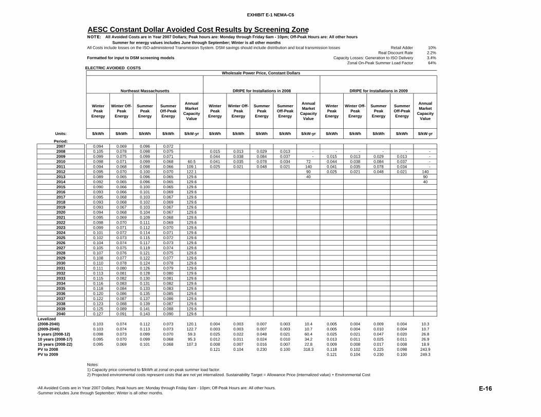
EXHIBIT E-1 NEMA-C$
AESC Constant Dollar Avoided Cost Results by Screening ZoneNOTE: All Avoided Costs are in Year 2007 Dollars; Peak hours are: Monday through Friday 6am - 10pm; Off-Peak Hours are: All other hours Summer for energy values includes June through September; Winter is all other monthsAll Costs include losses on the ISO-administered Transmission System. DSM savings should include distribution and local transmission losses Retail Adder 10%
Real Discount Rate 2.2%Formatted for input to DSM screening models Capacity Losses: Generation to ISO Delivery 3.4%
Zonal On-Peak Summer Load Factor 64%ELECTRIC AVOIDED COSTS
Winter Peak
Energy
Winter Off-Peak
Energy
Summer Peak
Energy
Summer Off-Peak Energy
Annual Market
Capacity Value
Winter Peak
Energy
Winter Off-Peak
Energy
Summer Peak
Energy
Summer Off-Peak Energy
Annual Market
Capacity Value
Winter Peak
Energy
Winter Off-Peak
Energy
Summer Peak
Energy
Summer Off-Peak Energy
Annual Market
Capacity Value
Units: $/kWh $/kWh $/kWh $/kWh $/kW-yr $/kWh $/kWh $/kWh $/kWh $/kW-yr $/kWh $/kWh $/kWh $/kWh $/kW-yr
Period:2007 0.094 0.069 0.096 0.0722008 0.105 0.078 0.098 0.075 0.015 0.013 0.029 0.013 - - - - - - 2009 0.099 0.075 0.099 0.071 0.044 0.038 0.084 0.037 - 0.015 0.013 0.029 0.013 - 2010 0.098 0.071 0.099 0.068 60.5 0.041 0.035 0.078 0.034 72 0.044 0.038 0.084 0.037 - 2011 0.094 0.068 0.098 0.066 109.1 0.025 0.021 0.048 0.021 140 0.041 0.035 0.078 0.034 - 2012 0.095 0.070 0.100 0.070 122.1 90 0.025 0.021 0.048 0.021 1402013 0.089 0.065 0.096 0.065 129.6 40 902014 0.092 0.065 0.096 0.065 129.6 402015 0.090 0.066 0.100 0.065 129.62016 0.093 0.066 0.101 0.069 129.62017 0.095 0.068 0.103 0.067 129.62018 0.093 0.068 0.102 0.069 129.62019 0.093 0.067 0.103 0.067 129.62020 0.094 0.068 0.104 0.067 129.62021 0.095 0.069 0.109 0.068 129.62022 0.098 0.070 0.111 0.069 129.62023 0.099 0.071 0.112 0.070 129.62024 0.101 0.072 0.114 0.071 129.62025 0.102 0.073 0.115 0.072 129.62026 0.104 0.074 0.117 0.073 129.62027 0.105 0.075 0.119 0.074 129.62028 0.107 0.076 0.121 0.075 129.62029 0.108 0.077 0.122 0.077 129.62030 0.110 0.078 0.124 0.078 129.62031 0.111 0.080 0.126 0.079 129.62032 0.113 0.081 0.128 0.080 129.62033 0.115 0.082 0.130 0.081 129.62034 0.116 0.083 0.131 0.082 129.62035 0.118 0.084 0.133 0.083 129.62036 0.120 0.086 0.135 0.085 129.62037 0.122 0.087 0.137 0.086 129.62038 0.123 0.088 0.139 0.087 129.62039 0.125 0.089 0.141 0.088 129.62040 0.127 0.091 0.143 0.090 129.6
Levelized(2008-2040) 0.103 0.074 0.112 0.073 120.1 0.004 0.003 0.007 0.003 10.4 0.005 0.004 0.009 0.004 10.3(2009-2040) 0.103 0.074 0.113 0.073 122.7 0.003 0.003 0.007 0.003 10.7 0.005 0.004 0.010 0.004 10.75 years (2008-12) 0.098 0.073 0.099 0.070 59.3 0.025 0.022 0.048 0.021 60.4 0.025 0.021 0.047 0.020 26.810 years (2008-17) 0.095 0.070 0.099 0.068 95.3 0.012 0.011 0.024 0.010 34.2 0.013 0.011 0.025 0.011 26.915 years (2008-22) 0.095 0.069 0.101 0.068 107.3 0.008 0.007 0.016 0.007 22.8 0.009 0.008 0.017 0.008 18.9PV to 2008 0.121 0.104 0.230 0.100 318.3 0.118 0.102 0.225 0.098 243.9PV to 2009 0.121 0.104 0.230 0.100 249.3
Notes: 1) Capacity price converted to $/kWh at zonal on-peak summer load factor.2) Projected environmental costs represent costs that are not yet internalized. Sustainability Target = Allowance Price (internalized value) + Environmental Cost
Wholesale Power Price, Constant Dollars
Northeast Massachusetts DRIPE for Installations in 2008 DRIPE for Installations in 2009
-All Avoided Costs are in Year 2007 Dollars; Peak hours are: Monday through Friday 6am - 10pm; Off-Peak Hours are: All other hours.-Summer includes June through September; Winter is all other months.
E-16
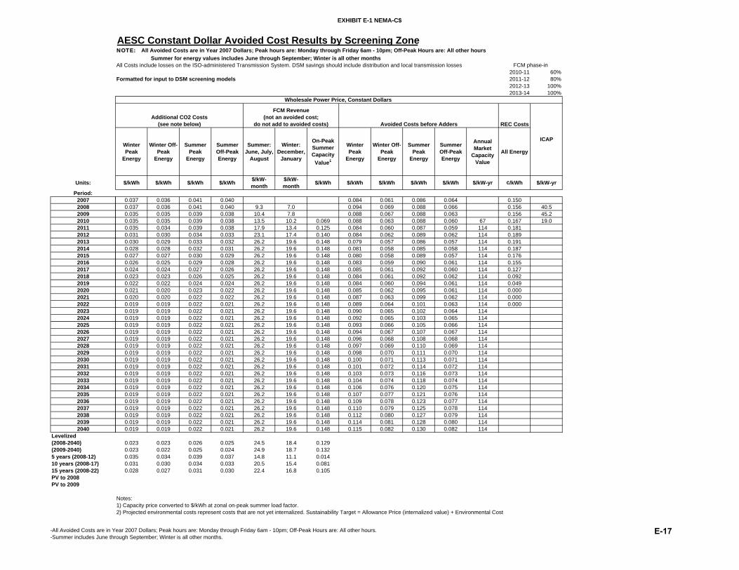
EXHIBIT E-1 NEMA-C$
Units:
Period:2007200820092010201120122013201420152016201720182019202020212022202320242025202620272028202920302031203220332034203520362037203820392040
Levelized(2008-2040)(2009-2040)5 years (2008-12)10 years (2008-17)15 years (2008-22)PV to 2008PV to 2009
AESC Constant Dollar Avoided Cost Results by Screening ZoneNOTE: All Avoided Costs are in Year 2007 Dollars; Peak hours are: Monday through Friday 6am - 10pm; Off-Peak Hours are: All other hours Summer for energy values includes June through September; Winter is all other monthsAll Costs include losses on the ISO-administered Transmission System. DSM savings should include distribution and local transmission losses
2010-11 60%Formatted for input to DSM screening models 2011-12 80%
2012-13 100%2013-14 100%
REC Costs
Winter Peak
Energy
Winter Off-Peak
Energy
Summer Peak
Energy
Summer Off-Peak Energy
Summer: June, July,
August
Winter: December,
January
On-Peak Summer Capacity Value1
Winter Peak
Energy
Winter Off-Peak
Energy
Summer Peak
Energy
Summer Off-Peak Energy
Annual Market
Capacity Value
All Energy
$/kWh $/kWh $/kWh $/kWh $/kW-month
$/kW-month $/kWh $/kWh $/kWh $/kWh $/kWh $/kW-yr ¢/kWh $/kW-yr
0.037 0.036 0.041 0.040 0.084 0.061 0.086 0.064 0.1500.037 0.036 0.041 0.040 9.3 7.0 0.094 0.069 0.088 0.066 0.156 40.50.035 0.035 0.039 0.038 10.4 7.8 0.088 0.067 0.088 0.063 0.156 45.20.035 0.035 0.039 0.038 13.5 10.2 0.069 0.088 0.063 0.088 0.060 67 0.167 19.00.035 0.034 0.039 0.038 17.9 13.4 0.125 0.084 0.060 0.087 0.059 114 0.1810.031 0.030 0.034 0.033 23.1 17.4 0.140 0.084 0.062 0.089 0.062 114 0.1890.030 0.029 0.033 0.032 26.2 19.6 0.148 0.079 0.057 0.086 0.057 114 0.1910.028 0.028 0.032 0.031 26.2 19.6 0.148 0.081 0.058 0.085 0.058 114 0.1870.027 0.027 0.030 0.029 26.2 19.6 0.148 0.080 0.058 0.089 0.057 114 0.1760.026 0.025 0.029 0.028 26.2 19.6 0.148 0.083 0.059 0.090 0.061 114 0.1550.024 0.024 0.027 0.026 26.2 19.6 0.148 0.085 0.061 0.092 0.060 114 0.1270.023 0.023 0.026 0.025 26.2 19.6 0.148 0.084 0.061 0.092 0.062 114 0.0920.022 0.022 0.024 0.024 26.2 19.6 0.148 0.084 0.060 0.094 0.061 114 0.0490.021 0.020 0.023 0.022 26.2 19.6 0.148 0.085 0.062 0.095 0.061 114 0.0000.020 0.020 0.022 0.022 26.2 19.6 0.148 0.087 0.063 0.099 0.062 114 0.0000.019 0.019 0.022 0.021 26.2 19.6 0.148 0.089 0.064 0.101 0.063 114 0.0000.019 0.019 0.022 0.021 26.2 19.6 0.148 0.090 0.065 0.102 0.064 1140.019 0.019 0.022 0.021 26.2 19.6 0.148 0.092 0.065 0.103 0.065 1140.019 0.019 0.022 0.021 26.2 19.6 0.148 0.093 0.066 0.105 0.066 1140.019 0.019 0.022 0.021 26.2 19.6 0.148 0.094 0.067 0.107 0.067 1140.019 0.019 0.022 0.021 26.2 19.6 0.148 0.096 0.068 0.108 0.068 1140.019 0.019 0.022 0.021 26.2 19.6 0.148 0.097 0.069 0.110 0.069 1140.019 0.019 0.022 0.021 26.2 19.6 0.148 0.098 0.070 0.111 0.070 1140.019 0.019 0.022 0.021 26.2 19.6 0.148 0.100 0.071 0.113 0.071 1140.019 0.019 0.022 0.021 26.2 19.6 0.148 0.101 0.072 0.114 0.072 1140.019 0.019 0.022 0.021 26.2 19.6 0.148 0.103 0.073 0.116 0.073 1140.019 0.019 0.022 0.021 26.2 19.6 0.148 0.104 0.074 0.118 0.074 1140.019 0.019 0.022 0.021 26.2 19.6 0.148 0.106 0.076 0.120 0.075 1140.019 0.019 0.022 0.021 26.2 19.6 0.148 0.107 0.077 0.121 0.076 1140.019 0.019 0.022 0.021 26.2 19.6 0.148 0.109 0.078 0.123 0.077 1140.019 0.019 0.022 0.021 26.2 19.6 0.148 0.110 0.079 0.125 0.078 1140.019 0.019 0.022 0.021 26.2 19.6 0.148 0.112 0.080 0.127 0.079 1140.019 0.019 0.022 0.021 26.2 19.6 0.148 0.114 0.081 0.128 0.080 1140.019 0.019 0.022 0.021 26.2 19.6 0.148 0.115 0.082 0.130 0.082 114
0.023 0.023 0.026 0.025 24.5 18.4 0.1290.023 0.022 0.025 0.024 24.9 18.7 0.1320.035 0.034 0.039 0.037 14.8 11.1 0.0140.031 0.030 0.034 0.033 20.5 15.4 0.0810.028 0.027 0.031 0.030 22.4 16.8 0.105
Notes: 1) Capacity price converted to $/kWh at zonal on-peak summer load factor.2) Projected environmental costs represent costs that are not yet internalized. Sustainability Target = Allowance Price (internalized value) + Environmental Cost
ICAP
Wholesale Power Price, Constant Dollars
FCM phase-in
FCM Revenue(not an avoided cost;
do not add to avoided costs) Avoided Costs before AddersAdditional CO2 Costs
(see note below)
-All Avoided Costs are in Year 2007 Dollars; Peak hours are: Monday through Friday 6am - 10pm; Off-Peak Hours are: All other hours.-Summer includes June through September; Winter is all other months.
E-17
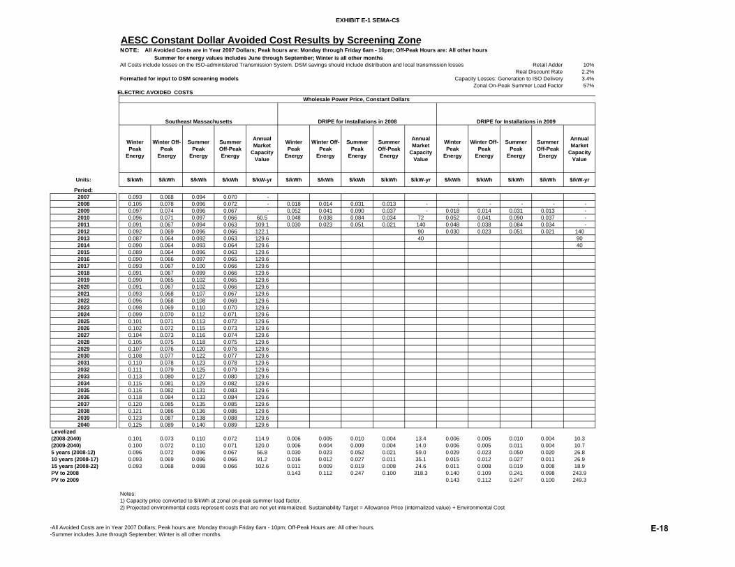
EXHIBIT E-1 SEMA-C$
AESC Constant Dollar Avoided Cost Results by Screening ZoneNOTE: All Avoided Costs are in Year 2007 Dollars; Peak hours are: Monday through Friday 6am - 10pm; Off-Peak Hours are: All other hours Summer for energy values includes June through September; Winter is all other monthsAll Costs include losses on the ISO-administered Transmission System. DSM savings should include distribution and local transmission losses Retail Adder 10%
Real Discount Rate 2.2%Formatted for input to DSM screening models Capacity Losses: Generation to ISO Delivery 3.4%
Zonal On-Peak Summer Load Factor 57%ELECTRIC AVOIDED COSTS
Winter Peak
Energy
Winter Off-Peak
Energy
Summer Peak
Energy
Summer Off-Peak Energy
Annual Market
Capacity Value
Winter Peak
Energy
Winter Off-Peak
Energy
Summer Peak
Energy
Summer Off-Peak Energy
Annual Market
Capacity Value
Winter Peak
Energy
Winter Off-Peak
Energy
Summer Peak
Energy
Summer Off-Peak Energy
Annual Market
Capacity Value
Units: $/kWh $/kWh $/kWh $/kWh $/kW-yr $/kWh $/kWh $/kWh $/kWh $/kW-yr $/kWh $/kWh $/kWh $/kWh $/kW-yr
Period:2007 0.093 0.068 0.094 0.070 - 2008 0.105 0.078 0.096 0.072 - 0.018 0.014 0.031 0.013 - - - - - - 2009 0.097 0.074 0.096 0.067 - 0.052 0.041 0.090 0.037 - 0.018 0.014 0.031 0.013 - 2010 0.096 0.071 0.097 0.066 60.5 0.048 0.038 0.084 0.034 72 0.052 0.041 0.090 0.037 - 2011 0.091 0.067 0.094 0.063 109.1 0.030 0.023 0.051 0.021 140 0.048 0.038 0.084 0.034 - 2012 0.092 0.069 0.096 0.066 122.1 90 0.030 0.023 0.051 0.021 1402013 0.087 0.064 0.092 0.063 129.6 40 902014 0.090 0.064 0.093 0.064 129.6 402015 0.089 0.064 0.096 0.063 129.62016 0.090 0.066 0.097 0.065 129.62017 0.093 0.067 0.100 0.066 129.62018 0.091 0.067 0.099 0.066 129.62019 0.090 0.065 0.102 0.065 129.62020 0.091 0.067 0.102 0.066 129.62021 0.093 0.068 0.107 0.067 129.62022 0.096 0.068 0.108 0.069 129.62023 0.098 0.069 0.110 0.070 129.62024 0.099 0.070 0.112 0.071 129.62025 0.101 0.071 0.113 0.072 129.62026 0.102 0.072 0.115 0.073 129.62027 0.104 0.073 0.116 0.074 129.62028 0.105 0.075 0.118 0.075 129.62029 0.107 0.076 0.120 0.076 129.62030 0.108 0.077 0.122 0.077 129.62031 0.110 0.078 0.123 0.078 129.62032 0.111 0.079 0.125 0.079 129.62033 0.113 0.080 0.127 0.080 129.62034 0.115 0.081 0.129 0.082 129.62035 0.116 0.082 0.131 0.083 129.62036 0.118 0.084 0.133 0.084 129.62037 0.120 0.085 0.135 0.085 129.62038 0.121 0.086 0.136 0.086 129.62039 0.123 0.087 0.138 0.088 129.62040 0.125 0.089 0.140 0.089 129.6
Levelized(2008-2040) 0.101 0.073 0.110 0.072 114.9 0.006 0.005 0.010 0.004 13.4 0.006 0.005 0.010 0.004 10.3(2009-2040) 0.100 0.072 0.110 0.071 120.0 0.006 0.004 0.009 0.004 14.0 0.006 0.005 0.011 0.004 10.75 years (2008-12) 0.096 0.072 0.096 0.067 56.8 0.030 0.023 0.052 0.021 59.0 0.029 0.023 0.050 0.020 26.810 years (2008-17) 0.093 0.069 0.096 0.066 91.2 0.016 0.012 0.027 0.011 35.1 0.015 0.012 0.027 0.011 26.915 years (2008-22) 0.093 0.068 0.098 0.066 102.6 0.011 0.009 0.019 0.008 24.6 0.011 0.008 0.019 0.008 18.9PV to 2008 0.143 0.112 0.247 0.100 318.3 0.140 0.109 0.241 0.098 243.9PV to 2009 0.143 0.112 0.247 0.100 249.3
Notes: 1) Capacity price converted to $/kWh at zonal on-peak summer load factor.2) Projected environmental costs represent costs that are not yet internalized. Sustainability Target = Allowance Price (internalized value) + Environmental Cost
Wholesale Power Price, Constant Dollars
Southeast Massachusetts DRIPE for Installations in 2008 DRIPE for Installations in 2009
-All Avoided Costs are in Year 2007 Dollars; Peak hours are: Monday through Friday 6am - 10pm; Off-Peak Hours are: All other hours.-Summer includes June through September; Winter is all other months.
E-18
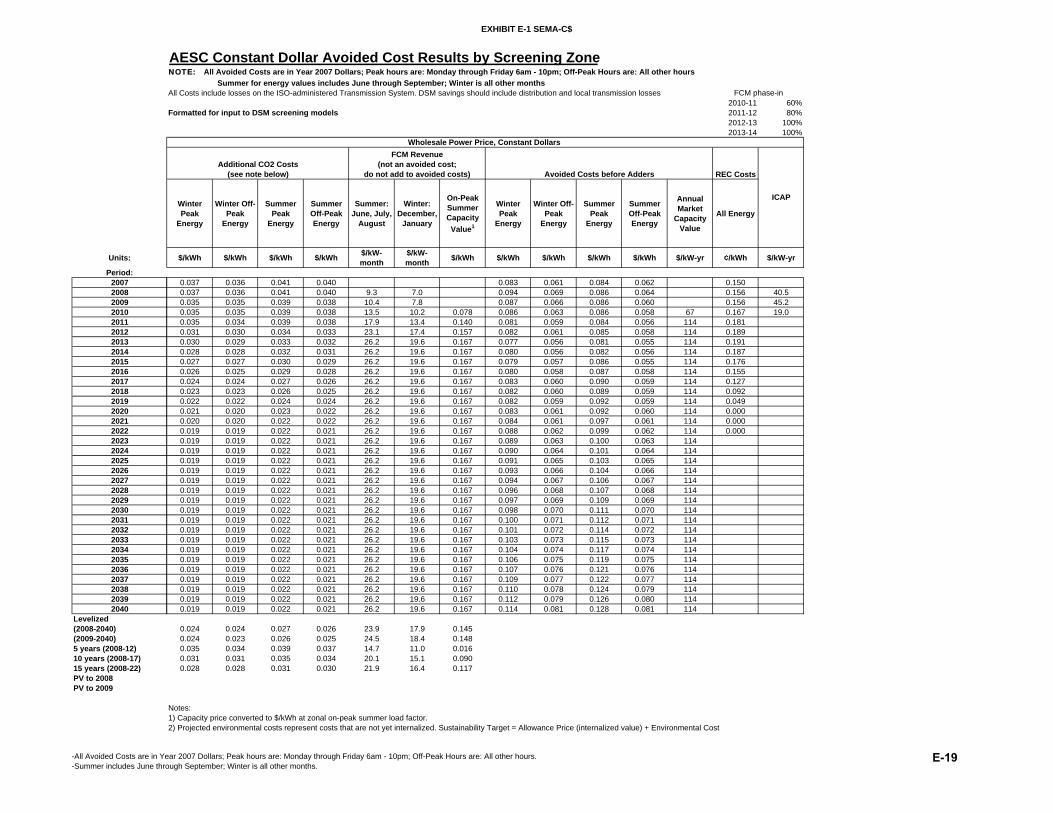
EXHIBIT E-1 SEMA-C$
Units:
Period:2007200820092010201120122013201420152016201720182019202020212022202320242025202620272028202920302031203220332034203520362037203820392040
Levelized(2008-2040)(2009-2040)5 years (2008-12)10 years (2008-17)15 years (2008-22)PV to 2008PV to 2009
AESC Constant Dollar Avoided Cost Results by Screening ZoneNOTE: All Avoided Costs are in Year 2007 Dollars; Peak hours are: Monday through Friday 6am - 10pm; Off-Peak Hours are: All other hours Summer for energy values includes June through September; Winter is all other monthsAll Costs include losses on the ISO-administered Transmission System. DSM savings should include distribution and local transmission losses
2010-11 60%Formatted for input to DSM screening models 2011-12 80%
2012-13 100%2013-14 100%
REC Costs
Winter Peak
Energy
Winter Off-Peak
Energy
Summer Peak
Energy
Summer Off-Peak Energy
Summer: June, July,
August
Winter: December,
January
On-Peak Summer Capacity Value1
Winter Peak
Energy
Winter Off-Peak
Energy
Summer Peak
Energy
Summer Off-Peak Energy
Annual Market
Capacity Value
All Energy
$/kWh $/kWh $/kWh $/kWh $/kW-month
$/kW-month $/kWh $/kWh $/kWh $/kWh $/kWh $/kW-yr ¢/kWh $/kW-yr
0.037 0.036 0.041 0.040 0.083 0.061 0.084 0.062 0.1500.037 0.036 0.041 0.040 9.3 7.0 0.094 0.069 0.086 0.064 0.156 40.50.035 0.035 0.039 0.038 10.4 7.8 0.087 0.066 0.086 0.060 0.156 45.20.035 0.035 0.039 0.038 13.5 10.2 0.078 0.086 0.063 0.086 0.058 67 0.167 19.00.035 0.034 0.039 0.038 17.9 13.4 0.140 0.081 0.059 0.084 0.056 114 0.1810.031 0.030 0.034 0.033 23.1 17.4 0.157 0.082 0.061 0.085 0.058 114 0.1890.030 0.029 0.033 0.032 26.2 19.6 0.167 0.077 0.056 0.081 0.055 114 0.1910.028 0.028 0.032 0.031 26.2 19.6 0.167 0.080 0.056 0.082 0.056 114 0.1870.027 0.027 0.030 0.029 26.2 19.6 0.167 0.079 0.057 0.086 0.055 114 0.1760.026 0.025 0.029 0.028 26.2 19.6 0.167 0.080 0.058 0.087 0.058 114 0.1550.024 0.024 0.027 0.026 26.2 19.6 0.167 0.083 0.060 0.090 0.059 114 0.1270.023 0.023 0.026 0.025 26.2 19.6 0.167 0.082 0.060 0.089 0.059 114 0.0920.022 0.022 0.024 0.024 26.2 19.6 0.167 0.082 0.059 0.092 0.059 114 0.0490.021 0.020 0.023 0.022 26.2 19.6 0.167 0.083 0.061 0.092 0.060 114 0.0000.020 0.020 0.022 0.022 26.2 19.6 0.167 0.084 0.061 0.097 0.061 114 0.0000.019 0.019 0.022 0.021 26.2 19.6 0.167 0.088 0.062 0.099 0.062 114 0.0000.019 0.019 0.022 0.021 26.2 19.6 0.167 0.089 0.063 0.100 0.063 1140.019 0.019 0.022 0.021 26.2 19.6 0.167 0.090 0.064 0.101 0.064 1140.019 0.019 0.022 0.021 26.2 19.6 0.167 0.091 0.065 0.103 0.065 1140.019 0.019 0.022 0.021 26.2 19.6 0.167 0.093 0.066 0.104 0.066 1140.019 0.019 0.022 0.021 26.2 19.6 0.167 0.094 0.067 0.106 0.067 1140.019 0.019 0.022 0.021 26.2 19.6 0.167 0.096 0.068 0.107 0.068 1140.019 0.019 0.022 0.021 26.2 19.6 0.167 0.097 0.069 0.109 0.069 1140.019 0.019 0.022 0.021 26.2 19.6 0.167 0.098 0.070 0.111 0.070 1140.019 0.019 0.022 0.021 26.2 19.6 0.167 0.100 0.071 0.112 0.071 1140.019 0.019 0.022 0.021 26.2 19.6 0.167 0.101 0.072 0.114 0.072 1140.019 0.019 0.022 0.021 26.2 19.6 0.167 0.103 0.073 0.115 0.073 1140.019 0.019 0.022 0.021 26.2 19.6 0.167 0.104 0.074 0.117 0.074 1140.019 0.019 0.022 0.021 26.2 19.6 0.167 0.106 0.075 0.119 0.075 1140.019 0.019 0.022 0.021 26.2 19.6 0.167 0.107 0.076 0.121 0.076 1140.019 0.019 0.022 0.021 26.2 19.6 0.167 0.109 0.077 0.122 0.077 1140.019 0.019 0.022 0.021 26.2 19.6 0.167 0.110 0.078 0.124 0.079 1140.019 0.019 0.022 0.021 26.2 19.6 0.167 0.112 0.079 0.126 0.080 1140.019 0.019 0.022 0.021 26.2 19.6 0.167 0.114 0.081 0.128 0.081 114
0.024 0.024 0.027 0.026 23.9 17.9 0.1450.024 0.023 0.026 0.025 24.5 18.4 0.1480.035 0.034 0.039 0.037 14.7 11.0 0.0160.031 0.031 0.035 0.034 20.1 15.1 0.0900.028 0.028 0.031 0.030 21.9 16.4 0.117
Notes: 1) Capacity price converted to $/kWh at zonal on-peak summer load factor.2) Projected environmental costs represent costs that are not yet internalized. Sustainability Target = Allowance Price (internalized value) + Environmental Cost
ICAP
Wholesale Power Price, Constant Dollars
FCM phase-in
FCM Revenue(not an avoided cost;
do not add to avoided costs) Avoided Costs before AddersAdditional CO2 Costs
(see note below)
-All Avoided Costs are in Year 2007 Dollars; Peak hours are: Monday through Friday 6am - 10pm; Off-Peak Hours are: All other hours.-Summer includes June through September; Winter is all other months.
E-19

EXHIBIT E-1 WCMA-C$
AESC Constant Dollar Avoided Cost Results by Screening ZoneNOTE: All Avoided Costs are in Year 2007 Dollars; Peak hours are: Monday through Friday 6am - 10pm; Off-Peak Hours are: All other hours Summer for energy values includes June through September; Winter is all other monthsAll Costs include losses on the ISO-administered Transmission System. DSM savings should include distribution and local transmission losses Retail Adder 10%
Real Discount Rate 2.2%Formatted for input to DSM screening models Capacity Losses: Generation to ISO Delivery 3.4%
Zonal On-Peak Summer Load Factor 60%ELECTRIC AVOIDED COSTS
Winter Peak
Energy
Winter Off-Peak
Energy
Summer Peak
Energy
Summer Off-Peak Energy
Annual Market
Capacity Value
Winter Peak
Energy
Winter Off-Peak
Energy
Summer Peak
Energy
Summer Off-Peak Energy
Annual Market
Capacity Value
Winter Peak
Energy
Winter Off-Peak
Energy
Summer Peak
Energy
Summer Off-Peak Energy
Annual Market
Capacity Value
Units: $/kWh $/kWh $/kWh $/kWh $/kW-yr $/kWh $/kWh $/kWh $/kWh $/kW-yr $/kWh $/kWh $/kWh $/kWh $/kW-yr
Period:2007 0.095 0.070 0.096 0.073 - 2008 0.106 0.080 0.098 0.076 - 0.015 0.012 0.026 0.010 - - - - - - 2009 0.098 0.076 0.097 0.072 - 0.045 0.034 0.076 0.029 - 0.015 0.012 0.026 0.010 - 2010 0.097 0.073 0.097 0.068 60.5 0.042 0.032 0.071 0.027 72 0.045 0.034 0.076 0.029 - 2011 0.093 0.070 0.096 0.066 109.1 0.025 0.019 0.043 0.016 140 0.042 0.032 0.071 0.027 - 2012 0.093 0.071 0.098 0.069 122.1 90 0.025 0.019 0.043 0.016 1402013 0.089 0.066 0.094 0.065 129.6 40 902014 0.092 0.066 0.094 0.066 129.6 402015 0.090 0.066 0.098 0.066 129.62016 0.092 0.067 0.098 0.069 129.62017 0.094 0.069 0.101 0.069 129.62018 0.091 0.068 0.099 0.068 129.62019 0.091 0.066 0.101 0.067 129.62020 0.093 0.069 0.103 0.068 129.62021 0.093 0.069 0.106 0.068 129.62022 0.096 0.070 0.108 0.070 129.62023 0.098 0.071 0.110 0.071 129.62024 0.099 0.072 0.112 0.072 129.62025 0.101 0.073 0.113 0.073 129.62026 0.102 0.074 0.115 0.074 129.62027 0.103 0.075 0.116 0.075 129.62028 0.105 0.076 0.118 0.076 129.62029 0.106 0.078 0.120 0.077 129.62030 0.108 0.079 0.122 0.078 129.62031 0.110 0.080 0.123 0.079 129.62032 0.111 0.081 0.125 0.081 129.62033 0.113 0.082 0.127 0.082 129.62034 0.114 0.083 0.129 0.083 129.62035 0.116 0.085 0.131 0.084 129.62036 0.118 0.086 0.133 0.085 129.62037 0.119 0.087 0.134 0.087 129.62038 0.121 0.088 0.136 0.088 129.62039 0.123 0.090 0.138 0.089 129.62040 0.125 0.091 0.140 0.090 129.6
Levelized(2008-2040) 0.101 0.074 0.110 0.074 114.9 0.005 0.004 0.009 0.003 13.4 0.005 0.004 0.009 0.003 10.3(2009-2040) 0.101 0.074 0.111 0.073 120.0 0.005 0.004 0.008 0.003 14.0 0.005 0.004 0.009 0.003 10.75 years (2008-12) 0.098 0.074 0.097 0.070 56.8 0.026 0.020 0.044 0.016 59.0 0.025 0.019 0.043 0.016 26.810 years (2008-17) 0.095 0.071 0.097 0.069 91.2 0.013 0.010 0.023 0.009 35.1 0.013 0.010 0.023 0.008 26.915 years (2008-22) 0.094 0.070 0.099 0.069 102.6 0.009 0.007 0.016 0.006 24.6 0.009 0.007 0.016 0.006 18.9PV to 2008 0.122 0.093 0.209 0.078 318.3 0.120 0.091 0.204 0.076 243.9PV to 2009 0.122 0.093 0.209 0.078 249.3
Notes: 1) Capacity price converted to $/kWh at zonal on-peak summer load factor.2) Projected environmental costs represent costs that are not yet internalized. Sustainability Target = Allowance Price (internalized value) + Environmental Cost
Wholesale Power Price, Constant Dollars
West-Central Massachusetts DRIPE for Installations in 2008 DRIPE for Installations in 2009
-All Avoided Costs are in Year 2007 Dollars; Peak hours are: Monday through Friday 6am - 10pm; Off-Peak Hours are: All other hours.-Summer includes June through September; Winter is all other months.
E-20

EXHIBIT E-1 WCMA-C$
Units:
Period:2007200820092010201120122013201420152016201720182019202020212022202320242025202620272028202920302031203220332034203520362037203820392040
Levelized(2008-2040)(2009-2040)5 years (2008-12)10 years (2008-17)15 years (2008-22)PV to 2008PV to 2009
AESC Constant Dollar Avoided Cost Results by Screening ZoneNOTE: All Avoided Costs are in Year 2007 Dollars; Peak hours are: Monday through Friday 6am - 10pm; Off-Peak Hours are: All other hours Summer for energy values includes June through September; Winter is all other monthsAll Costs include losses on the ISO-administered Transmission System. DSM savings should include distribution and local transmission losses
2010-11 60%Formatted for input to DSM screening models 2011-12 80%
2012-13 100%2013-14 100%
REC Costs
Winter Peak
Energy
Winter Off-Peak
Energy
Summer Peak
Energy
Summer Off-Peak Energy
Summer: June, July,
August
Winter: December,
January
On-Peak Summer Capacity Value1
Winter Peak
Energy
Winter Off-Peak
Energy
Summer Peak
Energy
Summer Off-Peak Energy
Annual Market
Capacity Value
All Energy
$/kWh $/kWh $/kWh $/kWh $/kW-month
$/kW-month $/kWh $/kWh $/kWh $/kWh $/kWh $/kW-yr ¢/kWh $/kW-yr
0.037 0.036 0.041 0.040 0.085 0.062 0.086 0.065 0.1500.037 0.036 0.041 0.040 9.3 7.0 0.095 0.071 0.087 0.067 0.156 40.50.035 0.035 0.039 0.038 10.4 7.8 0.087 0.068 0.086 0.064 0.156 45.20.035 0.035 0.039 0.038 13.5 10.2 0.074 0.087 0.064 0.087 0.060 67 0.167 19.00.035 0.034 0.039 0.038 17.9 13.4 0.133 0.083 0.062 0.086 0.058 114 0.1810.031 0.030 0.034 0.033 23.1 17.4 0.149 0.083 0.063 0.087 0.061 114 0.1890.030 0.029 0.033 0.032 26.2 19.6 0.158 0.079 0.058 0.083 0.057 114 0.1910.028 0.028 0.032 0.031 26.2 19.6 0.158 0.082 0.058 0.084 0.059 114 0.1870.027 0.027 0.030 0.029 26.2 19.6 0.158 0.080 0.058 0.087 0.058 114 0.1760.026 0.025 0.029 0.028 26.2 19.6 0.158 0.082 0.060 0.087 0.061 114 0.1550.024 0.024 0.027 0.026 26.2 19.6 0.158 0.084 0.062 0.091 0.061 114 0.1270.023 0.023 0.026 0.025 26.2 19.6 0.158 0.082 0.061 0.089 0.061 114 0.0920.022 0.022 0.024 0.024 26.2 19.6 0.158 0.082 0.060 0.091 0.060 114 0.0490.021 0.020 0.023 0.022 26.2 19.6 0.158 0.085 0.062 0.093 0.062 114 0.0000.020 0.020 0.022 0.022 26.2 19.6 0.158 0.085 0.062 0.097 0.062 114 0.0000.019 0.019 0.022 0.021 26.2 19.6 0.158 0.088 0.064 0.098 0.063 114 0.0000.019 0.019 0.022 0.021 26.2 19.6 0.158 0.089 0.065 0.100 0.064 1140.019 0.019 0.022 0.021 26.2 19.6 0.158 0.090 0.066 0.101 0.065 1140.019 0.019 0.022 0.021 26.2 19.6 0.158 0.091 0.067 0.103 0.066 1140.019 0.019 0.022 0.021 26.2 19.6 0.158 0.093 0.067 0.104 0.067 1140.019 0.019 0.022 0.021 26.2 19.6 0.158 0.094 0.068 0.106 0.068 1140.019 0.019 0.022 0.021 26.2 19.6 0.158 0.095 0.069 0.107 0.069 1140.019 0.019 0.022 0.021 26.2 19.6 0.158 0.097 0.070 0.109 0.070 1140.019 0.019 0.022 0.021 26.2 19.6 0.158 0.098 0.071 0.111 0.071 1140.019 0.019 0.022 0.021 26.2 19.6 0.158 0.100 0.073 0.112 0.072 1140.019 0.019 0.022 0.021 26.2 19.6 0.158 0.101 0.074 0.114 0.073 1140.019 0.019 0.022 0.021 26.2 19.6 0.158 0.103 0.075 0.115 0.074 1140.019 0.019 0.022 0.021 26.2 19.6 0.158 0.104 0.076 0.117 0.075 1140.019 0.019 0.022 0.021 26.2 19.6 0.158 0.106 0.077 0.119 0.076 1140.019 0.019 0.022 0.021 26.2 19.6 0.158 0.107 0.078 0.120 0.078 1140.019 0.019 0.022 0.021 26.2 19.6 0.158 0.109 0.079 0.122 0.079 1140.019 0.019 0.022 0.021 26.2 19.6 0.158 0.110 0.080 0.124 0.080 1140.019 0.019 0.022 0.021 26.2 19.6 0.158 0.112 0.081 0.126 0.081 1140.019 0.019 0.022 0.021 26.2 19.6 0.158 0.113 0.083 0.128 0.082 114
0.024 0.024 0.027 0.026 23.9 17.9 0.1380.024 0.023 0.026 0.025 24.5 18.4 0.1400.035 0.034 0.039 0.037 14.7 11.0 0.0150.031 0.031 0.035 0.034 20.1 15.1 0.0860.028 0.028 0.031 0.030 21.9 16.4 0.111
Notes: 1) Capacity price converted to $/kWh at zonal on-peak summer load factor.2) Projected environmental costs represent costs that are not yet internalized. Sustainability Target = Allowance Price (internalized value) + Environmental Cost
ICAP
Wholesale Power Price, Constant Dollars
FCM phase-in
FCM Revenue(not an avoided cost;
do not add to avoided costs) Avoided Costs before AddersAdditional CO2 Costs
(see note below)
-All Avoided Costs are in Year 2007 Dollars; Peak hours are: Monday through Friday 6am - 10pm; Off-Peak Hours are: All other hours.-Summer includes June through September; Winter is all other months.
E-21
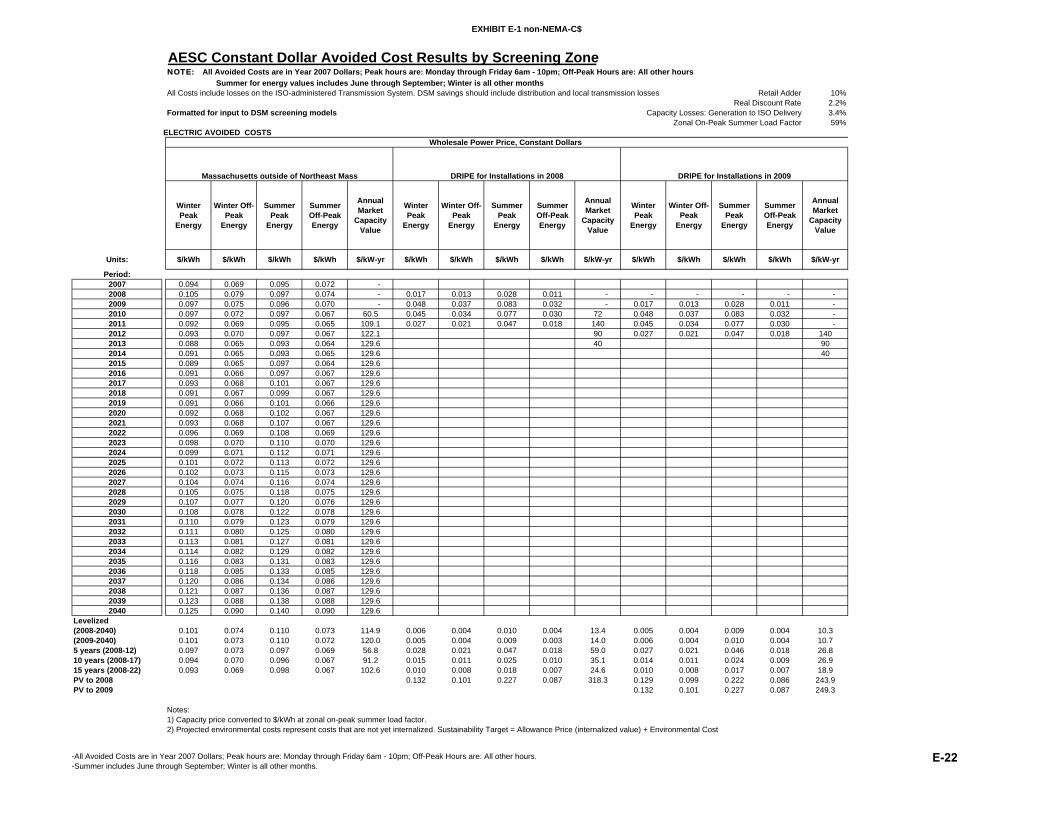
EXHIBIT E-1 non-NEMA-C$
AESC Constant Dollar Avoided Cost Results by Screening ZoneNOTE: All Avoided Costs are in Year 2007 Dollars; Peak hours are: Monday through Friday 6am - 10pm; Off-Peak Hours are: All other hours Summer for energy values includes June through September; Winter is all other monthsAll Costs include losses on the ISO-administered Transmission System. DSM savings should include distribution and local transmission losses Retail Adder 10%
Real Discount Rate 2.2%Formatted for input to DSM screening models Capacity Losses: Generation to ISO Delivery 3.4%
Zonal On-Peak Summer Load Factor 59%ELECTRIC AVOIDED COSTS
Winter Peak
Energy
Winter Off-Peak
Energy
Summer Peak
Energy
Summer Off-Peak Energy
Annual Market
Capacity Value
Winter Peak
Energy
Winter Off-Peak
Energy
Summer Peak
Energy
Summer Off-Peak Energy
Annual Market
Capacity Value
Winter Peak
Energy
Winter Off-Peak
Energy
Summer Peak
Energy
Summer Off-Peak Energy
Annual Market
Capacity Value
Units: $/kWh $/kWh $/kWh $/kWh $/kW-yr $/kWh $/kWh $/kWh $/kWh $/kW-yr $/kWh $/kWh $/kWh $/kWh $/kW-yr
Period:2007 0.094 0.069 0.095 0.072 - 2008 0.105 0.079 0.097 0.074 - 0.017 0.013 0.028 0.011 - - - - - - 2009 0.097 0.075 0.096 0.070 - 0.048 0.037 0.083 0.032 - 0.017 0.013 0.028 0.011 - 2010 0.097 0.072 0.097 0.067 60.5 0.045 0.034 0.077 0.030 72 0.048 0.037 0.083 0.032 - 2011 0.092 0.069 0.095 0.065 109.1 0.027 0.021 0.047 0.018 140 0.045 0.034 0.077 0.030 - 2012 0.093 0.070 0.097 0.067 122.1 90 0.027 0.021 0.047 0.018 1402013 0.088 0.065 0.093 0.064 129.6 40 902014 0.091 0.065 0.093 0.065 129.6 402015 0.089 0.065 0.097 0.064 129.62016 0.091 0.066 0.097 0.067 129.62017 0.093 0.068 0.101 0.067 129.62018 0.091 0.067 0.099 0.067 129.62019 0.091 0.066 0.101 0.066 129.62020 0.092 0.068 0.102 0.067 129.62021 0.093 0.068 0.107 0.067 129.62022 0.096 0.069 0.108 0.069 129.62023 0.098 0.070 0.110 0.070 129.62024 0.099 0.071 0.112 0.071 129.62025 0.101 0.072 0.113 0.072 129.62026 0.102 0.073 0.115 0.073 129.62027 0.104 0.074 0.116 0.074 129.62028 0.105 0.075 0.118 0.075 129.62029 0.107 0.077 0.120 0.076 129.62030 0.108 0.078 0.122 0.078 129.62031 0.110 0.079 0.123 0.079 129.62032 0.111 0.080 0.125 0.080 129.62033 0.113 0.081 0.127 0.081 129.62034 0.114 0.082 0.129 0.082 129.62035 0.116 0.083 0.131 0.083 129.62036 0.118 0.085 0.133 0.085 129.62037 0.120 0.086 0.134 0.086 129.62038 0.121 0.087 0.136 0.087 129.62039 0.123 0.088 0.138 0.088 129.62040 0.125 0.090 0.140 0.090 129.6
Levelized(2008-2040) 0.101 0.074 0.110 0.073 114.9 0.006 0.004 0.010 0.004 13.4 0.005 0.004 0.009 0.004 10.3(2009-2040) 0.101 0.073 0.110 0.072 120.0 0.005 0.004 0.009 0.003 14.0 0.006 0.004 0.010 0.004 10.75 years (2008-12) 0.097 0.073 0.097 0.069 56.8 0.028 0.021 0.047 0.018 59.0 0.027 0.021 0.046 0.018 26.810 years (2008-17) 0.094 0.070 0.096 0.067 91.2 0.015 0.011 0.025 0.010 35.1 0.014 0.011 0.024 0.009 26.915 years (2008-22) 0.093 0.069 0.098 0.067 102.6 0.010 0.008 0.018 0.007 24.6 0.010 0.008 0.017 0.007 18.9PV to 2008 0.132 0.101 0.227 0.087 318.3 0.129 0.099 0.222 0.086 243.9PV to 2009 0.132 0.101 0.227 0.087 249.3
Notes: 1) Capacity price converted to $/kWh at zonal on-peak summer load factor.2) Projected environmental costs represent costs that are not yet internalized. Sustainability Target = Allowance Price (internalized value) + Environmental Cost
Wholesale Power Price, Constant Dollars
Massachusetts outside of Northeast Mass DRIPE for Installations in 2008 DRIPE for Installations in 2009
-All Avoided Costs are in Year 2007 Dollars; Peak hours are: Monday through Friday 6am - 10pm; Off-Peak Hours are: All other hours.-Summer includes June through September; Winter is all other months.
E-22
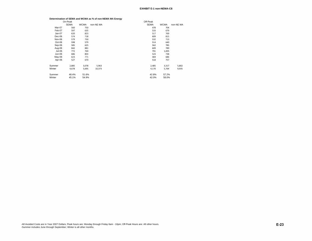
EXHIBIT E-1 non-NEMA-C$
Determination of SEMA and WCMA as % of non-NEMA MA EnergyOn-Peak Off-Peak
SEMA WCMA non-NE MA SEMA WCMA non-NE MAMar-07 560 750 478 704 Feb-07 597 635 533 679 Jan-07 620 823 517 769 Dec-06 574 718 609 815 Nov-06 579 750 532 713 Oct-06 598 579 514 640 Sep-06 585 625 562 785 Aug-06 842 881 609 789 Jul-06 772 769 791 1,005
Jun-06 686 803 524 738 May-06 623 771 469 686 Apr-06 527 670 518 757
Summer 2,885 3,078 5,963 2,485 3,317 5,802 Winter 4,678 5,695 10,373 4,170 5,764 9,935
Summer 48.4% 51.6% 42.8% 57.2%Winter 45.1% 54.9% 42.0% 58.0%
-All Avoided Costs are in Year 2007 Dollars; Peak hours are: Monday through Friday 6am - 10pm; Off-Peak Hours are: All other hours.-Summer includes June through September; Winter is all other months.
E-23
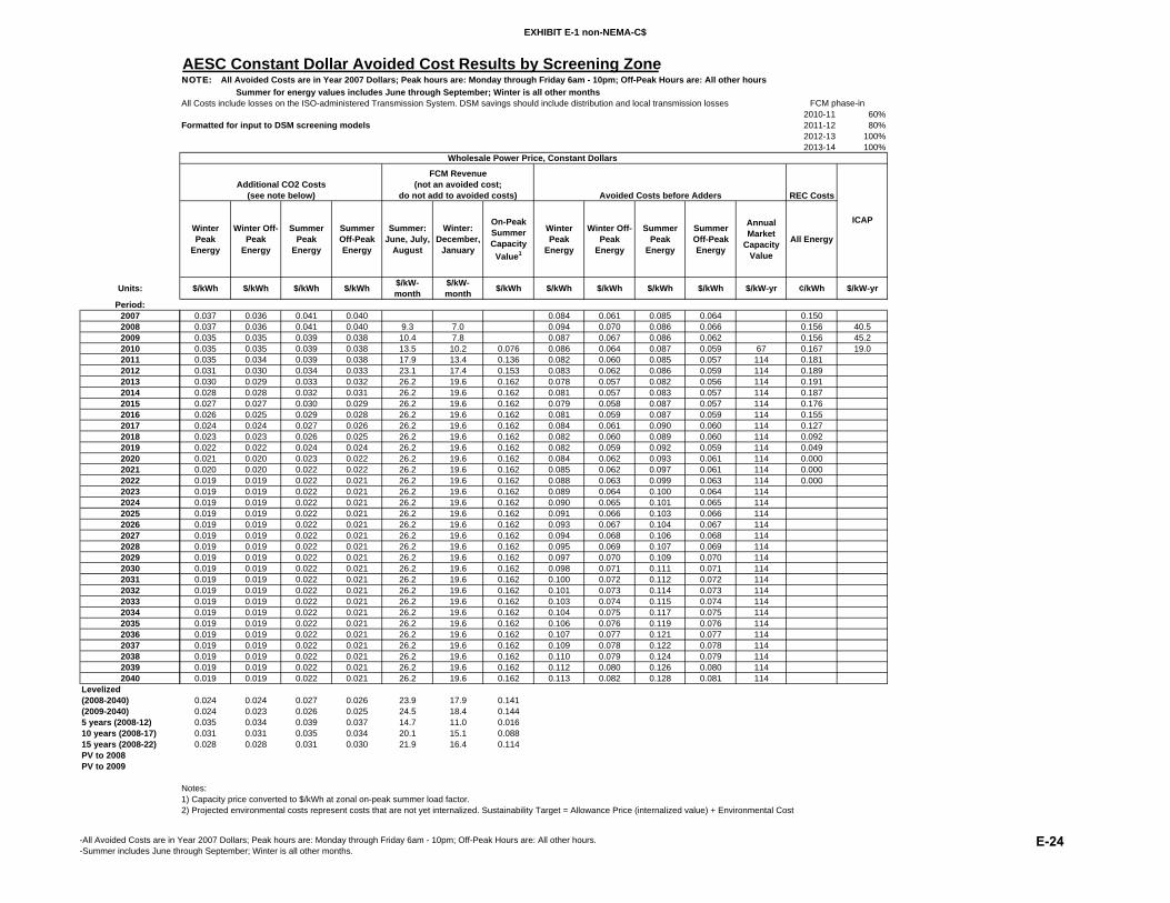
EXHIBIT E-1 non-NEMA-C$
Units:
Period:2007200820092010201120122013201420152016201720182019202020212022202320242025202620272028202920302031203220332034203520362037203820392040
Levelized(2008-2040)(2009-2040)5 years (2008-12)10 years (2008-17)15 years (2008-22)PV to 2008PV to 2009
AESC Constant Dollar Avoided Cost Results by Screening ZoneNOTE: All Avoided Costs are in Year 2007 Dollars; Peak hours are: Monday through Friday 6am - 10pm; Off-Peak Hours are: All other hours Summer for energy values includes June through September; Winter is all other monthsAll Costs include losses on the ISO-administered Transmission System. DSM savings should include distribution and local transmission losses
2010-11 60%Formatted for input to DSM screening models 2011-12 80%
2012-13 100%2013-14 100%
REC Costs
Winter Peak
Energy
Winter Off-Peak
Energy
Summer Peak
Energy
Summer Off-Peak Energy
Summer: June, July,
August
Winter: December,
January
On-Peak Summer Capacity Value1
Winter Peak
Energy
Winter Off-Peak
Energy
Summer Peak
Energy
Summer Off-Peak Energy
Annual Market
Capacity Value
All Energy
$/kWh $/kWh $/kWh $/kWh $/kW-month
$/kW-month $/kWh $/kWh $/kWh $/kWh $/kWh $/kW-yr ¢/kWh $/kW-yr
0.037 0.036 0.041 0.040 0.084 0.061 0.085 0.064 0.1500.037 0.036 0.041 0.040 9.3 7.0 0.094 0.070 0.086 0.066 0.156 40.50.035 0.035 0.039 0.038 10.4 7.8 0.087 0.067 0.086 0.062 0.156 45.20.035 0.035 0.039 0.038 13.5 10.2 0.076 0.086 0.064 0.087 0.059 67 0.167 19.00.035 0.034 0.039 0.038 17.9 13.4 0.136 0.082 0.060 0.085 0.057 114 0.1810.031 0.030 0.034 0.033 23.1 17.4 0.153 0.083 0.062 0.086 0.059 114 0.1890.030 0.029 0.033 0.032 26.2 19.6 0.162 0.078 0.057 0.082 0.056 114 0.1910.028 0.028 0.032 0.031 26.2 19.6 0.162 0.081 0.057 0.083 0.057 114 0.1870.027 0.027 0.030 0.029 26.2 19.6 0.162 0.079 0.058 0.087 0.057 114 0.1760.026 0.025 0.029 0.028 26.2 19.6 0.162 0.081 0.059 0.087 0.059 114 0.1550.024 0.024 0.027 0.026 26.2 19.6 0.162 0.084 0.061 0.090 0.060 114 0.1270.023 0.023 0.026 0.025 26.2 19.6 0.162 0.082 0.060 0.089 0.060 114 0.0920.022 0.022 0.024 0.024 26.2 19.6 0.162 0.082 0.059 0.092 0.059 114 0.0490.021 0.020 0.023 0.022 26.2 19.6 0.162 0.084 0.062 0.093 0.061 114 0.0000.020 0.020 0.022 0.022 26.2 19.6 0.162 0.085 0.062 0.097 0.061 114 0.0000.019 0.019 0.022 0.021 26.2 19.6 0.162 0.088 0.063 0.099 0.063 114 0.0000.019 0.019 0.022 0.021 26.2 19.6 0.162 0.089 0.064 0.100 0.064 1140.019 0.019 0.022 0.021 26.2 19.6 0.162 0.090 0.065 0.101 0.065 1140.019 0.019 0.022 0.021 26.2 19.6 0.162 0.091 0.066 0.103 0.066 1140.019 0.019 0.022 0.021 26.2 19.6 0.162 0.093 0.067 0.104 0.067 1140.019 0.019 0.022 0.021 26.2 19.6 0.162 0.094 0.068 0.106 0.068 1140.019 0.019 0.022 0.021 26.2 19.6 0.162 0.095 0.069 0.107 0.069 1140.019 0.019 0.022 0.021 26.2 19.6 0.162 0.097 0.070 0.109 0.070 1140.019 0.019 0.022 0.021 26.2 19.6 0.162 0.098 0.071 0.111 0.071 1140.019 0.019 0.022 0.021 26.2 19.6 0.162 0.100 0.072 0.112 0.072 1140.019 0.019 0.022 0.021 26.2 19.6 0.162 0.101 0.073 0.114 0.073 1140.019 0.019 0.022 0.021 26.2 19.6 0.162 0.103 0.074 0.115 0.074 1140.019 0.019 0.022 0.021 26.2 19.6 0.162 0.104 0.075 0.117 0.075 1140.019 0.019 0.022 0.021 26.2 19.6 0.162 0.106 0.076 0.119 0.076 1140.019 0.019 0.022 0.021 26.2 19.6 0.162 0.107 0.077 0.121 0.077 1140.019 0.019 0.022 0.021 26.2 19.6 0.162 0.109 0.078 0.122 0.078 1140.019 0.019 0.022 0.021 26.2 19.6 0.162 0.110 0.079 0.124 0.079 1140.019 0.019 0.022 0.021 26.2 19.6 0.162 0.112 0.080 0.126 0.080 1140.019 0.019 0.022 0.021 26.2 19.6 0.162 0.113 0.082 0.128 0.081 114
0.024 0.024 0.027 0.026 23.9 17.9 0.1410.024 0.023 0.026 0.025 24.5 18.4 0.1440.035 0.034 0.039 0.037 14.7 11.0 0.0160.031 0.031 0.035 0.034 20.1 15.1 0.0880.028 0.028 0.031 0.030 21.9 16.4 0.114
Notes: 1) Capacity price converted to $/kWh at zonal on-peak summer load factor.2) Projected environmental costs represent costs that are not yet internalized. Sustainability Target = Allowance Price (internalized value) + Environmental Cost
ICAP
Wholesale Power Price, Constant Dollars
FCM phase-in
FCM Revenue(not an avoided cost;
do not add to avoided costs) Avoided Costs before AddersAdditional CO2 Costs
(see note below)
-All Avoided Costs are in Year 2007 Dollars; Peak hours are: Monday through Friday 6am - 10pm; Off-Peak Hours are: All other hours.-Summer includes June through September; Winter is all other months.
E-24

EXHIBIT E-1 SWCT-C$
AESC Constant Dollar Avoided Cost Results by Screening ZoneNOTE: All Avoided Costs are in Year 2007 Dollars; Peak hours are: Monday through Friday 6am - 10pm; Off-Peak Hours are: All other hours Summer for energy values includes June through September; Winter is all other monthsAll Costs include losses on the ISO-administered Transmission System. DSM savings should include distribution and local transmission losses Retail Adder 10%
Real Discount Rate 2.2%Formatted for input to DSM screening models Capacity Losses: Generation to ISO Delivery 3.4%
Zonal On-Peak Summer Load Factor 60%ELECTRIC AVOIDED COSTS
Winter Peak
Energy
Winter Off-Peak
Energy
Summer Peak
Energy
Summer Off-Peak Energy
Annual Market
Capacity Value
Winter Peak
Energy
Winter Off-Peak
Energy
Summer Peak
Energy
Summer Off-Peak Energy
Annual Market
Capacity Value
Winter Peak
Energy
Winter Off-Peak
Energy
Summer Peak
Energy
Summer Off-Peak Energy
Annual Market
Capacity Value
Units: $/kWh $/kWh $/kWh $/kWh $/kW-yr $/kWh $/kWh $/kWh $/kWh $/kW-yr $/kWh $/kWh $/kWh $/kWh $/kW-yr
Period:2007 0.100 0.073 0.105 0.0762008 0.112 0.083 0.107 0.081 0.017 0.013 0.033 0.016 - - - - - - 2009 0.105 0.080 0.108 0.074 0.049 0.039 0.100 0.051 - 0.017 0.013 0.033 0.016 - 2010 0.102 0.076 0.105 0.072 60.5 0.046 0.037 0.097 0.050 72 0.049 0.039 0.100 0.051 - 2011 0.097 0.071 0.104 0.069 109.1 0.028 0.023 0.059 0.030 140 0.046 0.037 0.097 0.050 - 2012 0.098 0.073 0.108 0.070 122.1 90 0.028 0.023 0.059 0.030 1402013 0.094 0.067 0.101 0.066 129.6 40 902014 0.095 0.067 0.100 0.067 129.6 402015 0.093 0.067 0.100 0.066 129.62016 0.094 0.068 0.103 0.067 129.62017 0.098 0.070 0.107 0.070 129.62018 0.096 0.071 0.105 0.070 129.62019 0.095 0.069 0.105 0.069 129.62020 0.097 0.071 0.109 0.070 129.62021 0.097 0.072 0.111 0.070 129.62022 0.100 0.072 0.114 0.072 129.62023 0.102 0.073 0.116 0.073 129.62024 0.103 0.074 0.118 0.074 129.62025 0.105 0.075 0.119 0.075 129.62026 0.106 0.076 0.121 0.076 129.62027 0.108 0.077 0.123 0.077 129.62028 0.110 0.079 0.125 0.078 129.62029 0.111 0.080 0.127 0.079 129.62030 0.113 0.081 0.128 0.081 129.62031 0.114 0.082 0.130 0.082 129.62032 0.116 0.083 0.132 0.083 129.62033 0.118 0.084 0.134 0.084 129.62034 0.119 0.086 0.136 0.085 129.62035 0.121 0.087 0.138 0.087 129.62036 0.123 0.088 0.140 0.088 129.62037 0.125 0.089 0.142 0.089 129.62038 0.126 0.091 0.144 0.090 129.62039 0.128 0.092 0.146 0.092 129.62040 0.130 0.093 0.148 0.093 129.6
Levelized(2008-2040) 0.106 0.077 0.117 0.076 120.1 0.004 0.003 0.009 0.004 10.4 0.006 0.004 0.012 0.006 10.3(2009-2040) 0.105 0.076 0.117 0.075 122.7 0.004 0.003 0.008 0.004 10.7 0.006 0.005 0.012 0.006 10.75 years (2008-12) 0.103 0.077 0.106 0.073 59.3 0.028 0.023 0.058 0.029 60.4 0.028 0.022 0.057 0.029 26.810 years (2008-17) 0.099 0.073 0.104 0.070 95.3 0.014 0.011 0.029 0.015 34.2 0.015 0.012 0.030 0.015 26.915 years (2008-22) 0.098 0.072 0.106 0.070 107.3 0.009 0.008 0.019 0.010 22.8 0.010 0.008 0.021 0.011 18.9PV to 2008 0.135 0.109 0.279 0.141 318.3 0.132 0.106 0.273 0.138 243.9PV to 2009 0.135 0.109 0.279 0.141 249.3
Notes: 1) Capacity price converted to $/kWh at zonal on-peak summer load factor.2) Projected environmental costs represent costs that are not yet internalized. Sustainability Target = Allowance Price (internalized value) + Environmental Cost
Wholesale Power Price, Constant Dollars
Southwest Connecticut DRIPE for Installations in 2008 DRIPE for Installations in 2009
-All Avoided Costs are in Year 2007 Dollars; Peak hours are: Monday through Friday 6am - 10pm; Off-Peak Hours are: All other hours.-Summer includes June through September; Winter is all other months.
E-25

EXHIBIT E-1 SWCT-C$
Units:
Period:2007200820092010201120122013201420152016201720182019202020212022202320242025202620272028202920302031203220332034203520362037203820392040
Levelized(2008-2040)(2009-2040)5 years (2008-12)10 years (2008-17)15 years (2008-22)PV to 2008PV to 2009
AESC Constant Dollar Avoided Cost Results by Screening ZoneNOTE: All Avoided Costs are in Year 2007 Dollars; Peak hours are: Monday through Friday 6am - 10pm; Off-Peak Hours are: All other hours Summer for energy values includes June through September; Winter is all other monthsAll Costs include losses on the ISO-administered Transmission System. DSM savings should include distribution and local transmission losses
2010-11 60%Formatted for input to DSM screening models 2011-12 80%
2012-13 100%2013-14 100%
REC Costs
Winter Peak
Energy
Winter Off-Peak
Energy
Summer Peak
Energy
Summer Off-Peak Energy
Summer: June, July,
August
Winter: December,
January
On-Peak Summer Capacity Value1
Winter Peak
Energy
Winter Off-Peak
Energy
Summer Peak
Energy
Summer Off-Peak Energy
Annual Market
Capacity Value
All Energy
$/kWh $/kWh $/kWh $/kWh $/kW-month
$/kW-month $/kWh $/kWh $/kWh $/kWh $/kWh $/kW-yr ¢/kWh $/kW-yr
0.037 0.036 0.041 0.040 0.089 0.065 0.094 0.068 0.1750.037 0.036 0.041 0.040 9.3 7.0 0.099 0.073 0.095 0.071 0.222 40.50.035 0.035 0.039 0.038 10.4 7.8 0.093 0.070 0.096 0.065 0.233 45.20.035 0.035 0.039 0.038 13.5 10.2 0.074 0.090 0.067 0.093 0.063 67 0.233 19.00.035 0.034 0.039 0.038 17.9 13.4 0.133 0.087 0.063 0.092 0.061 114 0.2110.031 0.030 0.034 0.033 23.1 17.4 0.148 0.087 0.064 0.096 0.062 114 0.1890.030 0.029 0.033 0.032 26.2 19.6 0.158 0.083 0.059 0.090 0.059 114 0.1670.028 0.028 0.032 0.031 26.2 19.6 0.158 0.085 0.059 0.090 0.059 114 0.1450.027 0.027 0.030 0.029 26.2 19.6 0.158 0.083 0.060 0.090 0.058 114 0.1230.026 0.025 0.029 0.028 26.2 19.6 0.158 0.085 0.061 0.093 0.060 114 0.0990.024 0.024 0.027 0.026 26.2 19.6 0.158 0.088 0.063 0.097 0.063 114 0.0740.023 0.023 0.026 0.025 26.2 19.6 0.158 0.087 0.064 0.095 0.063 114 0.0490.022 0.022 0.024 0.024 26.2 19.6 0.158 0.086 0.062 0.095 0.062 114 0.0250.021 0.020 0.023 0.022 26.2 19.6 0.158 0.088 0.065 0.099 0.063 114 0.0000.020 0.020 0.022 0.022 26.2 19.6 0.158 0.088 0.065 0.101 0.063 114 0.0000.019 0.019 0.022 0.021 26.2 19.6 0.158 0.091 0.065 0.104 0.065 114 0.0000.019 0.019 0.022 0.021 26.2 19.6 0.158 0.093 0.066 0.106 0.066 1140.019 0.019 0.022 0.021 26.2 19.6 0.158 0.094 0.067 0.107 0.067 1140.019 0.019 0.022 0.021 26.2 19.6 0.158 0.095 0.068 0.109 0.068 1140.019 0.019 0.022 0.021 26.2 19.6 0.158 0.097 0.069 0.110 0.069 1140.019 0.019 0.022 0.021 26.2 19.6 0.158 0.098 0.070 0.112 0.070 1140.019 0.019 0.022 0.021 26.2 19.6 0.158 0.100 0.071 0.113 0.071 1140.019 0.019 0.022 0.021 26.2 19.6 0.158 0.101 0.072 0.115 0.072 1140.019 0.019 0.022 0.021 26.2 19.6 0.158 0.102 0.073 0.117 0.073 1140.019 0.019 0.022 0.021 26.2 19.6 0.158 0.104 0.075 0.118 0.074 1140.019 0.019 0.022 0.021 26.2 19.6 0.158 0.105 0.076 0.120 0.075 1140.019 0.019 0.022 0.021 26.2 19.6 0.158 0.107 0.077 0.122 0.076 1140.019 0.019 0.022 0.021 26.2 19.6 0.158 0.109 0.078 0.124 0.078 1140.019 0.019 0.022 0.021 26.2 19.6 0.158 0.110 0.079 0.125 0.079 1140.019 0.019 0.022 0.021 26.2 19.6 0.158 0.112 0.080 0.127 0.080 1140.019 0.019 0.022 0.021 26.2 19.6 0.158 0.113 0.081 0.129 0.081 1140.019 0.019 0.022 0.021 26.2 19.6 0.158 0.115 0.082 0.131 0.082 1140.019 0.019 0.022 0.021 26.2 19.6 0.158 0.117 0.084 0.133 0.083 1140.019 0.019 0.022 0.021 26.2 19.6 0.158 0.118 0.085 0.135 0.085 114
0.023 0.023 0.026 0.025 24.5 18.4 0.1370.023 0.022 0.025 0.024 24.9 18.7 0.1400.035 0.034 0.039 0.037 14.8 11.1 0.0150.031 0.030 0.034 0.033 20.5 15.4 0.0860.028 0.027 0.031 0.030 22.4 16.8 0.111
Notes: 1) Capacity price converted to $/kWh at zonal on-peak summer load factor.2) Projected environmental costs represent costs that are not yet internalized. Sustainability Target = Allowance Price (internalized value) + Environmental Cost
ICAP
Wholesale Power Price, Constant Dollars
FCM phase-in
FCM Revenue(not an avoided cost;
do not add to avoided costs) Avoided Costs before AddersAdditional CO2 Costs
(see note below)
-All Avoided Costs are in Year 2007 Dollars; Peak hours are: Monday through Friday 6am - 10pm; Off-Peak Hours are: All other hours.-Summer includes June through September; Winter is all other months.
E-26

EXHIBIT E-1 NS-C$
AESC Constant Dollar Avoided Cost Results by Screening ZoneNOTE: All Avoided Costs are in Year 2007 Dollars; Peak hours are: Monday through Friday 6am - 10pm; Off-Peak Hours are: All other hours Summer for energy values includes June through September; Winter is all other monthsAll Costs include losses on the ISO-administered Transmission System. DSM savings should include distribution and local transmission losses Retail Adder 10%
Real Discount Rate 2.2%Formatted for input to DSM screening models Capacity Losses: Generation to ISO Delivery 3.4%
Zonal On-Peak Summer Load Factor 59%ELECTRIC AVOIDED COSTS
Winter Peak
Energy
Winter Off-Peak
Energy
Summer Peak
Energy
Summer Off-Peak Energy
Annual Market
Capacity Value
Winter Peak
Energy
Winter Off-Peak
Energy
Summer Peak
Energy
Summer Off-Peak Energy
Annual Market
Capacity Value
Winter Peak
Energy
Winter Off-Peak
Energy
Summer Peak
Energy
Summer Off-Peak Energy
Annual Market
Capacity Value
Units: $/kWh $/kWh $/kWh $/kWh $/kW-yr $/kWh $/kWh $/kWh $/kWh $/kW-yr $/kWh $/kWh $/kWh $/kWh $/kW-yr
Period:2007 0.104 0.075 0.116 0.078 - 2008 0.116 0.085 0.118 0.082 - 0.017 0.013 0.033 0.016 - - - - - - 2009 0.109 0.082 0.118 0.076 - 0.049 0.039 0.100 0.051 - 0.017 0.013 0.033 0.016 - 2010 0.102 0.076 0.110 0.072 60.5 0.046 0.037 0.097 0.050 72 0.049 0.039 0.100 0.051 - 2011 0.097 0.071 0.109 0.069 109.1 0.028 0.023 0.059 0.030 140 0.046 0.037 0.097 0.050 - 2012 0.098 0.073 0.113 0.070 122.1 90 0.028 0.023 0.059 0.030 1402013 0.094 0.067 0.106 0.066 129.6 40 902014 0.095 0.067 0.105 0.067 129.6 402015 0.093 0.067 0.105 0.066 129.62016 0.094 0.068 0.108 0.067 129.62017 0.098 0.070 0.112 0.070 129.62018 0.096 0.071 0.110 0.070 129.62019 0.095 0.069 0.111 0.069 129.62020 0.097 0.071 0.115 0.070 129.62021 0.097 0.072 0.116 0.070 129.62022 0.100 0.072 0.120 0.072 129.62023 0.102 0.073 0.122 0.073 129.62024 0.103 0.074 0.124 0.074 129.62025 0.105 0.075 0.125 0.075 129.62026 0.106 0.076 0.127 0.076 129.62027 0.108 0.077 0.129 0.077 129.62028 0.110 0.079 0.131 0.078 129.62029 0.111 0.080 0.133 0.079 129.62030 0.113 0.081 0.135 0.081 129.62031 0.114 0.082 0.137 0.082 129.62032 0.116 0.083 0.139 0.083 129.62033 0.118 0.084 0.141 0.084 129.62034 0.119 0.086 0.143 0.085 129.62035 0.121 0.087 0.145 0.087 129.62036 0.123 0.088 0.147 0.088 129.62037 0.125 0.089 0.149 0.089 129.62038 0.126 0.091 0.151 0.090 129.62039 0.128 0.092 0.153 0.092 129.62040 0.130 0.093 0.156 0.093 129.6
Levelized(2008-2040) 0.106 0.077 0.123 0.076 114.9 0.006 0.005 0.012 0.006 13.4 0.006 0.004 0.012 0.006 10.3(2009-2040) 0.106 0.076 0.123 0.075 120.0 0.005 0.004 0.011 0.005 14.0 0.006 0.005 0.012 0.006 10.75 years (2008-12) 0.105 0.077 0.114 0.074 56.8 0.028 0.023 0.058 0.030 59.0 0.028 0.022 0.057 0.029 26.810 years (2008-17) 0.100 0.073 0.111 0.071 91.2 0.015 0.012 0.031 0.016 35.1 0.015 0.012 0.030 0.015 26.915 years (2008-22) 0.099 0.072 0.112 0.071 102.6 0.010 0.008 0.022 0.011 24.6 0.010 0.008 0.021 0.011 18.9PV to 2008 0.135 0.109 0.279 0.141 318.3 0.132 0.106 0.273 0.138 243.9PV to 2009 0.135 0.109 0.279 0.141 249.3
Notes: 1) Capacity price converted to $/kWh at zonal on-peak summer load factor.2) Projected environmental costs represent costs that are not yet internalized. Sustainability Target = Allowance Price (internalized value) + Environmental Cost
Wholesale Power Price, Constant Dollars
Norwalk-Stamford DRIPE for Installations in 2008 DRIPE for Installations in 2009
-All Avoided Costs are in Year 2007 Dollars; Peak hours are: Monday through Friday 6am - 10pm; Off-Peak Hours are: All other hours.-Summer includes June through September; Winter is all other months.
E-27

EXHIBIT E-1 NS-C$
Units:
Period:2007200820092010201120122013201420152016201720182019202020212022202320242025202620272028202920302031203220332034203520362037203820392040
Levelized(2008-2040)(2009-2040)5 years (2008-12)10 years (2008-17)15 years (2008-22)PV to 2008PV to 2009
AESC Constant Dollar Avoided Cost Results by Screening ZoneNOTE: All Avoided Costs are in Year 2007 Dollars; Peak hours are: Monday through Friday 6am - 10pm; Off-Peak Hours are: All other hours Summer for energy values includes June through September; Winter is all other monthsAll Costs include losses on the ISO-administered Transmission System. DSM savings should include distribution and local transmission losses
2010-11 60%Formatted for input to DSM screening models 2011-12 80%
2012-13 100%2013-14 100%
REC Costs
Winter Peak
Energy
Winter Off-Peak
Energy
Summer Peak
Energy
Summer Off-Peak Energy
Summer: June, July,
August
Winter: December,
January
On-Peak Summer Capacity Value1
Winter Peak
Energy
Winter Off-Peak
Energy
Summer Peak
Energy
Summer Off-Peak Energy
Annual Market
Capacity Value
All Energy
$/kWh $/kWh $/kWh $/kWh $/kW-month
$/kW-month $/kWh $/kWh $/kWh $/kWh $/kWh $/kW-yr ¢/kWh $/kW-yr
0.037 0.036 0.041 0.040 0.093 0.066 0.104 0.069 0.1750.037 0.036 0.041 0.040 9.3 7.0 0.103 0.075 0.105 0.073 0.222 40.50.035 0.035 0.039 0.038 10.4 7.8 0.096 0.072 0.105 0.067 0.233 45.20.035 0.035 0.039 0.038 13.5 10.2 0.075 0.090 0.067 0.097 0.063 67 0.233 19.00.035 0.034 0.039 0.038 17.9 13.4 0.135 0.087 0.063 0.097 0.061 114 0.2110.031 0.030 0.034 0.033 23.1 17.4 0.152 0.087 0.064 0.101 0.062 114 0.1890.030 0.029 0.033 0.032 26.2 19.6 0.161 0.083 0.059 0.095 0.059 114 0.1670.028 0.028 0.032 0.031 26.2 19.6 0.161 0.085 0.059 0.094 0.059 114 0.1450.027 0.027 0.030 0.029 26.2 19.6 0.161 0.083 0.060 0.095 0.058 114 0.1230.026 0.025 0.029 0.028 26.2 19.6 0.161 0.085 0.061 0.097 0.060 114 0.0990.024 0.024 0.027 0.026 26.2 19.6 0.161 0.088 0.063 0.101 0.063 114 0.0740.023 0.023 0.026 0.025 26.2 19.6 0.161 0.087 0.064 0.099 0.063 114 0.0490.022 0.022 0.024 0.024 26.2 19.6 0.161 0.086 0.062 0.100 0.062 114 0.0250.021 0.020 0.023 0.022 26.2 19.6 0.161 0.088 0.065 0.104 0.063 114 0.0000.020 0.020 0.022 0.022 26.2 19.6 0.161 0.088 0.065 0.106 0.063 114 0.0000.019 0.019 0.022 0.021 26.2 19.6 0.161 0.091 0.065 0.109 0.065 114 0.0000.019 0.019 0.022 0.021 26.2 19.6 0.161 0.093 0.066 0.111 0.066 1140.019 0.019 0.022 0.021 26.2 19.6 0.161 0.094 0.067 0.112 0.067 1140.019 0.019 0.022 0.021 26.2 19.6 0.161 0.095 0.068 0.114 0.068 1140.019 0.019 0.022 0.021 26.2 19.6 0.161 0.097 0.069 0.116 0.069 1140.019 0.019 0.022 0.021 26.2 19.6 0.161 0.098 0.070 0.117 0.070 1140.019 0.019 0.022 0.021 26.2 19.6 0.161 0.100 0.071 0.119 0.071 1140.019 0.019 0.022 0.021 26.2 19.6 0.161 0.101 0.072 0.121 0.072 1140.019 0.019 0.022 0.021 26.2 19.6 0.161 0.102 0.073 0.123 0.073 1140.019 0.019 0.022 0.021 26.2 19.6 0.161 0.104 0.075 0.124 0.074 1140.019 0.019 0.022 0.021 26.2 19.6 0.161 0.105 0.076 0.126 0.075 1140.019 0.019 0.022 0.021 26.2 19.6 0.161 0.107 0.077 0.128 0.076 1140.019 0.019 0.022 0.021 26.2 19.6 0.161 0.109 0.078 0.130 0.078 1140.019 0.019 0.022 0.021 26.2 19.6 0.161 0.110 0.079 0.132 0.079 1140.019 0.019 0.022 0.021 26.2 19.6 0.161 0.112 0.080 0.134 0.080 1140.019 0.019 0.022 0.021 26.2 19.6 0.161 0.113 0.081 0.136 0.081 1140.019 0.019 0.022 0.021 26.2 19.6 0.161 0.115 0.082 0.137 0.082 1140.019 0.019 0.022 0.021 26.2 19.6 0.161 0.117 0.084 0.139 0.083 1140.019 0.019 0.022 0.021 26.2 19.6 0.161 0.118 0.085 0.142 0.085 114
0.024 0.024 0.027 0.026 23.9 17.9 0.1400.024 0.023 0.026 0.025 24.5 18.4 0.1430.035 0.034 0.039 0.037 14.7 11.0 0.0160.031 0.031 0.035 0.034 20.1 15.1 0.0870.028 0.028 0.031 0.030 21.9 16.4 0.113
Notes: 1) Capacity price converted to $/kWh at zonal on-peak summer load factor.2) Projected environmental costs represent costs that are not yet internalized. Sustainability Target = Allowance Price (internalized value) + Environmental Cost
Wholesale Power Price, Constant Dollars FCM Revenue
(not an avoided cost; do not add to avoided costs)
FCM phase-in
Avoided Costs before AddersAdditional CO2 Costs
(see note below)
ICAP
-All Avoided Costs are in Year 2007 Dollars; Peak hours are: Monday through Friday 6am - 10pm; Off-Peak Hours are: All other hours.-Summer includes June through September; Winter is all other months.
E-28

EXHIBIT E-1 SW-NS-C$
AESC Constant Dollar Avoided Cost Results by Screening ZoneNOTE: All Avoided Costs are in Year 2007 Dollars; Peak hours are: Monday through Friday 6am - 10pm; Off-Peak Hours are: All other hours Summer for energy values includes June through September; Winter is all other monthsAll Costs include losses on the ISO-administered Transmission System. DSM savings should include distribution and local transmission losses Retail Adder 10%
Real Discount Rate 2.2%Formatted for input to DSM screening models Capacity Losses: Generation to ISO Delivery 3.4%
Zonal On-Peak Summer Load Factor 61%ELECTRIC AVOIDED COSTS
Winter Peak
Energy
Winter Off-Peak
Energy
Summer Peak
Energy
Summer Off-Peak Energy
Annual Market
Capacity Value
Winter Peak
Energy
Winter Off-Peak
Energy
Summer Peak
Energy
Summer Off-Peak Energy
Annual Market
Capacity Value
Winter Peak
Energy
Winter Off-Peak
Energy
Summer Peak
Energy
Summer Off-Peak Energy
Annual Market
Capacity Value
Units: $/kWh $/kWh $/kWh $/kWh $/kW-yr $/kWh $/kWh $/kWh $/kWh $/kW-yr $/kWh $/kWh $/kWh $/kWh $/kW-yr
Period:2007 0.098 0.073 0.100 0.076 - 2008 0.109 0.082 0.102 0.080 - 0.017 0.013 0.033 0.016 - - - - - - 2009 0.102 0.079 0.102 0.074 - 0.049 0.039 0.100 0.051 - 0.017 0.013 0.033 0.016 - 2010 0.102 0.076 0.102 0.072 60.5 0.046 0.037 0.097 0.050 72 0.049 0.039 0.100 0.051 - 2011 0.097 0.071 0.101 0.069 109.1 0.028 0.023 0.059 0.030 140 0.046 0.037 0.097 0.050 - 2012 0.098 0.073 0.105 0.070 122.1 90 0.028 0.023 0.059 0.030 1402013 0.094 0.067 0.098 0.066 129.6 40 902014 0.095 0.067 0.098 0.067 129.6 402015 0.093 0.067 0.098 0.066 129.62016 0.094 0.068 0.100 0.067 129.62017 0.098 0.070 0.104 0.070 129.62018 0.096 0.071 0.102 0.070 129.62019 0.095 0.069 0.102 0.069 129.62020 0.097 0.071 0.106 0.070 129.62021 0.097 0.072 0.108 0.070 129.62022 0.100 0.072 0.111 0.072 129.62023 0.102 0.073 0.113 0.073 129.62024 0.103 0.074 0.115 0.074 129.62025 0.105 0.075 0.116 0.075 129.62026 0.106 0.076 0.118 0.076 129.62027 0.108 0.077 0.120 0.077 129.62028 0.110 0.079 0.121 0.078 129.62029 0.111 0.080 0.123 0.079 129.62030 0.113 0.081 0.125 0.081 129.62031 0.114 0.082 0.127 0.082 129.62032 0.116 0.083 0.129 0.083 129.62033 0.118 0.084 0.130 0.084 129.62034 0.119 0.086 0.132 0.085 129.62035 0.121 0.087 0.134 0.087 129.62036 0.123 0.088 0.136 0.088 129.62037 0.125 0.089 0.138 0.089 129.62038 0.126 0.091 0.140 0.090 129.62039 0.128 0.092 0.142 0.092 129.62040 0.130 0.093 0.144 0.093 129.6
Levelized(2008-2040) 0.106 0.077 0.114 0.076 114.9 0.006 0.005 0.012 0.006 13.4 0.006 0.004 0.012 0.006 10.3(2009-2040) 0.105 0.076 0.114 0.075 120.0 0.005 0.004 0.011 0.005 14.0 0.006 0.005 0.012 0.006 10.75 years (2008-12) 0.102 0.076 0.102 0.073 56.8 0.028 0.023 0.058 0.030 59.0 0.028 0.022 0.057 0.029 26.810 years (2008-17) 0.099 0.072 0.101 0.070 91.2 0.015 0.012 0.031 0.016 35.1 0.015 0.012 0.030 0.015 26.915 years (2008-22) 0.098 0.072 0.102 0.070 102.6 0.010 0.008 0.022 0.011 24.6 0.010 0.008 0.021 0.011 18.9PV to 2008 0.135 0.109 0.279 0.141 318.3 0.132 0.106 0.273 0.138 243.9PV to 2009 0.135 0.109 0.279 0.141 249.3
Notes: 1) Capacity price converted to $/kWh at zonal on-peak summer load factor.2) Projected environmental costs represent costs that are not yet internalized. Sustainability Target = Allowance Price (internalized value) + Environmental Cost
Wholesale Power Price, Constant Dollars
Southwest Connecticut except Norwalk-Stamford DRIPE for Installations in 2008 DRIPE for Installations in 2009
-All Avoided Costs are in Year 2007 Dollars; Peak hours are: Monday through Friday 6am - 10pm; Off-Peak Hours are: All other hours.-Summer includes June through September; Winter is all other months.
E-29

EXHIBIT E-1 SW-NS-C$
Units:
Period:2007200820092010201120122013201420152016201720182019202020212022202320242025202620272028202920302031203220332034203520362037203820392040
Levelized(2008-2040)(2009-2040)5 years (2008-12)10 years (2008-17)15 years (2008-22)PV to 2008PV to 2009
AESC Constant Dollar Avoided Cost Results by Screening ZoneNOTE: All Avoided Costs are in Year 2007 Dollars; Peak hours are: Monday through Friday 6am - 10pm; Off-Peak Hours are: All other hours Summer for energy values includes June through September; Winter is all other monthsAll Costs include losses on the ISO-administered Transmission System. DSM savings should include distribution and local transmission losses
2010-11 60%Formatted for input to DSM screening models 2011-12 80%
2012-13 100%2013-14 100%
REC Costs
Winter Peak
Energy
Winter Off-Peak
Energy
Summer Peak
Energy
Summer Off-Peak Energy
Summer: June, July,
August
Winter: December,
January
On-Peak Summer Capacity Value1
Winter Peak
Energy
Winter Off-Peak
Energy
Summer Peak
Energy
Summer Off-Peak Energy
Annual Market
Capacity Value
All Energy
$/kWh $/kWh $/kWh $/kWh $/kW-month
$/kW-month $/kWh $/kWh $/kWh $/kWh $/kWh $/kW-yr ¢/kWh $/kW-yr
0.037 0.036 0.041 0.040 0.088 0.064 0.089 0.067 0.1750.037 0.036 0.041 0.040 9.3 7.0 0.097 0.073 0.090 0.071 0.222 40.50.035 0.035 0.039 0.038 10.4 7.8 0.091 0.070 0.090 0.065 0.233 45.20.035 0.035 0.039 0.038 13.5 10.2 0.073 0.090 0.067 0.090 0.063 67 0.233 19.00.035 0.034 0.039 0.038 17.9 13.4 0.131 0.087 0.063 0.090 0.061 114 0.2110.031 0.030 0.034 0.033 23.1 17.4 0.147 0.087 0.064 0.093 0.062 114 0.1890.030 0.029 0.033 0.032 26.2 19.6 0.156 0.083 0.059 0.088 0.059 114 0.1670.028 0.028 0.032 0.031 26.2 19.6 0.156 0.085 0.059 0.087 0.059 114 0.1450.027 0.027 0.030 0.029 26.2 19.6 0.156 0.083 0.060 0.088 0.058 114 0.1230.026 0.025 0.029 0.028 26.2 19.6 0.156 0.085 0.061 0.090 0.060 114 0.0990.024 0.024 0.027 0.026 26.2 19.6 0.156 0.088 0.063 0.094 0.063 114 0.0740.023 0.023 0.026 0.025 26.2 19.6 0.156 0.087 0.064 0.092 0.063 114 0.0490.022 0.022 0.024 0.024 26.2 19.6 0.156 0.086 0.062 0.093 0.062 114 0.0250.021 0.020 0.023 0.022 26.2 19.6 0.156 0.088 0.065 0.097 0.063 114 0.0000.020 0.020 0.022 0.022 26.2 19.6 0.156 0.088 0.065 0.098 0.063 114 0.0000.019 0.019 0.022 0.021 26.2 19.6 0.156 0.091 0.065 0.101 0.065 114 0.0000.019 0.019 0.022 0.021 26.2 19.6 0.156 0.093 0.066 0.103 0.066 1140.019 0.019 0.022 0.021 26.2 19.6 0.156 0.094 0.067 0.104 0.067 1140.019 0.019 0.022 0.021 26.2 19.6 0.156 0.095 0.068 0.106 0.068 1140.019 0.019 0.022 0.021 26.2 19.6 0.156 0.097 0.069 0.107 0.069 1140.019 0.019 0.022 0.021 26.2 19.6 0.156 0.098 0.070 0.109 0.070 1140.019 0.019 0.022 0.021 26.2 19.6 0.156 0.100 0.071 0.110 0.071 1140.019 0.019 0.022 0.021 26.2 19.6 0.156 0.101 0.072 0.112 0.072 1140.019 0.019 0.022 0.021 26.2 19.6 0.156 0.102 0.073 0.114 0.073 1140.019 0.019 0.022 0.021 26.2 19.6 0.156 0.104 0.075 0.115 0.074 1140.019 0.019 0.022 0.021 26.2 19.6 0.156 0.105 0.076 0.117 0.075 1140.019 0.019 0.022 0.021 26.2 19.6 0.156 0.107 0.077 0.119 0.076 1140.019 0.019 0.022 0.021 26.2 19.6 0.156 0.109 0.078 0.120 0.078 1140.019 0.019 0.022 0.021 26.2 19.6 0.156 0.110 0.079 0.122 0.079 1140.019 0.019 0.022 0.021 26.2 19.6 0.156 0.112 0.080 0.124 0.080 1140.019 0.019 0.022 0.021 26.2 19.6 0.156 0.113 0.081 0.126 0.081 1140.019 0.019 0.022 0.021 26.2 19.6 0.156 0.115 0.082 0.127 0.082 1140.019 0.019 0.022 0.021 26.2 19.6 0.156 0.117 0.084 0.129 0.083 1140.019 0.019 0.022 0.021 26.2 19.6 0.156 0.118 0.085 0.131 0.085 114
0.024 0.024 0.027 0.026 23.9 17.9 0.1360.024 0.023 0.026 0.025 24.5 18.4 0.1390.035 0.034 0.039 0.037 14.7 11.0 0.0150.031 0.031 0.035 0.034 20.1 15.1 0.0850.028 0.028 0.031 0.030 21.9 16.4 0.110
Notes: 1) Capacity price converted to $/kWh at zonal on-peak summer load factor.2) Projected environmental costs represent costs that are not yet internalized. Sustainability Target = Allowance Price (internalized value) + Environmental Cost
Wholesale Power Price, Constant Dollars
FCM Revenue(not an avoided cost;
do not add to avoided costs)
FCM phase-in
Avoided Costs before AddersAdditional CO2 Costs
(see note below)
ICAP
-All Avoided Costs are in Year 2007 Dollars; Peak hours are: Monday through Friday 6am - 10pm; Off-Peak Hours are: All other hours.-Summer includes June through September; Winter is all other months.
E-30

EXHIBIT E-1 non-SWCT-C$
AESC Constant Dollar Avoided Cost Results by Screening ZoneNOTE: All Avoided Costs are in Year 2007 Dollars; Peak hours are: Monday through Friday 6am - 10pm; Off-Peak Hours are: All other hours Summer for energy values includes June through September; Winter is all other monthsAll Costs include losses on the ISO-administered Transmission System. DSM savings should include distribution and local transmission losses Retail Adder 10%
Real Discount Rate 2.2%Formatted for input to DSM screening models Capacity Losses: Generation to ISO Delivery 3.4%
Zonal On-Peak Summer Load Factor 60%ELECTRIC AVOIDED COSTS
Winter Peak
Energy
Winter Off-Peak
Energy
Summer Peak
Energy
Summer Off-Peak Energy
Annual Market
Capacity Value
Winter Peak
Energy
Winter Off-Peak
Energy
Summer Peak
Energy
Summer Off-Peak Energy
Annual Market
Capacity Value
Winter Peak
Energy
Winter Off-Peak
Energy
Summer Peak
Energy
Summer Off-Peak Energy
Annual Market
Capacity Value
Units: $/kWh $/kWh $/kWh $/kWh $/kW-yr $/kWh $/kWh $/kWh $/kWh $/kW-yr $/kWh $/kWh $/kWh $/kWh $/kW-yr
Period:2007 0.099 0.072 0.104 0.075 - 2008 0.110 0.082 0.105 0.080 - 0.017 0.013 0.033 0.016 - - - - - - 2009 0.103 0.079 0.106 0.073 - 0.049 0.039 0.100 0.051 - 0.017 0.013 0.033 0.016 - 2010 0.100 0.075 0.103 0.071 60.5 0.046 0.037 0.097 0.050 72 0.049 0.039 0.100 0.051 - 2011 0.096 0.070 0.102 0.068 109.1 0.028 0.023 0.059 0.030 140 0.046 0.037 0.097 0.050 - 2012 0.097 0.072 0.105 0.069 122.1 90 0.028 0.023 0.059 0.030 1402013 0.092 0.066 0.100 0.065 129.6 40 902014 0.094 0.066 0.099 0.066 129.6 402015 0.091 0.066 0.100 0.065 129.62016 0.092 0.067 0.101 0.066 129.62017 0.096 0.069 0.105 0.068 129.62018 0.094 0.069 0.103 0.069 129.62019 0.093 0.068 0.104 0.067 129.62020 0.095 0.070 0.107 0.069 129.62021 0.096 0.070 0.108 0.069 129.62022 0.099 0.071 0.112 0.071 129.62023 0.101 0.072 0.114 0.072 129.62024 0.102 0.073 0.115 0.073 129.62025 0.103 0.074 0.117 0.074 129.62026 0.105 0.075 0.119 0.075 129.62027 0.106 0.077 0.121 0.076 129.62028 0.108 0.078 0.122 0.077 129.62029 0.110 0.079 0.124 0.078 129.62030 0.111 0.080 0.126 0.079 129.62031 0.113 0.081 0.128 0.080 129.62032 0.114 0.082 0.130 0.082 129.62033 0.116 0.083 0.131 0.083 129.62034 0.118 0.085 0.133 0.084 129.62035 0.119 0.086 0.135 0.085 129.62036 0.121 0.087 0.137 0.086 129.62037 0.123 0.088 0.139 0.088 129.62038 0.125 0.090 0.141 0.089 129.62039 0.127 0.091 0.143 0.090 129.62040 0.128 0.092 0.145 0.091 129.6
Levelized(2008-2040) 0.104 0.076 0.115 0.074 114.9 0.006 0.005 0.012 0.006 13.4 0.006 0.004 0.012 0.006 10.3(2009-2040) 0.104 0.075 0.115 0.074 120.0 0.005 0.004 0.011 0.005 14.0 0.006 0.005 0.012 0.006 10.75 years (2008-12) 0.101 0.076 0.104 0.072 56.8 0.028 0.023 0.058 0.030 59.0 0.028 0.022 0.057 0.029 26.810 years (2008-17) 0.097 0.071 0.102 0.069 91.2 0.015 0.012 0.031 0.016 35.1 0.015 0.012 0.030 0.015 26.915 years (2008-22) 0.097 0.071 0.104 0.069 102.6 0.010 0.008 0.022 0.011 24.6 0.010 0.008 0.021 0.011 18.9PV to 2008 0.135 0.109 0.279 0.141 318.3 0.132 0.106 0.273 0.138 243.9PV to 2009 0.135 0.109 0.279 0.141 249.3
Notes: 1) Capacity price converted to $/kWh at zonal on-peak summer load factor.2) Projected environmental costs represent costs that are not yet internalized. Sustainability Target = Allowance Price (internalized value) + Environmental Cost
Wholesale Power Price, Constant Dollars
Connecticut except Southwest Connecticut DRIPE for Installations in 2008 DRIPE for Installations in 2009
-All Avoided Costs are in Year 2007 Dollars; Peak hours are: Monday through Friday 6am - 10pm; Off-Peak Hours are: All other hours.-Summer includes June through September; Winter is all other months.
E-31

EXHIBIT E-1 non-SWCT-C$
Units:
Period:2007200820092010201120122013201420152016201720182019202020212022202320242025202620272028202920302031203220332034203520362037203820392040
Levelized(2008-2040)(2009-2040)5 years (2008-12)10 years (2008-17)15 years (2008-22)PV to 2008PV to 2009
AESC Constant Dollar Avoided Cost Results by Screening ZoneNOTE: All Avoided Costs are in Year 2007 Dollars; Peak hours are: Monday through Friday 6am - 10pm; Off-Peak Hours are: All other hours Summer for energy values includes June through September; Winter is all other monthsAll Costs include losses on the ISO-administered Transmission System. DSM savings should include distribution and local transmission losses
2010-11 60%Formatted for input to DSM screening models 2011-12 80%
2012-13 100%2013-14 100%
REC Costs
Winter Peak
Energy
Winter Off-Peak
Energy
Summer Peak
Energy
Summer Off-Peak Energy
Summer: June, July,
August
Winter: December,
January
On-Peak Summer Capacity Value1
Winter Peak
Energy
Winter Off-Peak
Energy
Summer Peak
Energy
Summer Off-Peak Energy
Annual Market
Capacity Value
All Energy
$/kWh $/kWh $/kWh $/kWh $/kW-month
$/kW-month $/kWh $/kWh $/kWh $/kWh $/kWh $/kW-yr ¢/kWh $/kW-yr
0.037 0.036 0.041 0.040 0.088 0.064 0.092 0.066 0.1750.037 0.036 0.041 0.040 9.3 7.0 0.098 0.072 0.093 0.071 0.222 40.50.035 0.035 0.039 0.038 10.4 7.8 0.091 0.069 0.094 0.064 0.233 45.20.035 0.035 0.039 0.038 13.5 10.2 0.074 0.089 0.065 0.091 0.062 67 0.233 19.00.035 0.034 0.039 0.038 17.9 13.4 0.133 0.085 0.062 0.090 0.060 114 0.2110.031 0.030 0.034 0.033 23.1 17.4 0.148 0.086 0.063 0.094 0.060 114 0.1890.030 0.029 0.033 0.032 26.2 19.6 0.158 0.082 0.058 0.089 0.057 114 0.1670.028 0.028 0.032 0.031 26.2 19.6 0.158 0.084 0.059 0.088 0.058 114 0.1450.027 0.027 0.030 0.029 26.2 19.6 0.158 0.082 0.059 0.089 0.057 114 0.1230.026 0.025 0.029 0.028 26.2 19.6 0.158 0.083 0.060 0.091 0.059 114 0.0990.024 0.024 0.027 0.026 26.2 19.6 0.158 0.086 0.062 0.094 0.062 114 0.0740.023 0.023 0.026 0.025 26.2 19.6 0.158 0.085 0.062 0.093 0.062 114 0.0490.022 0.022 0.024 0.024 26.2 19.6 0.158 0.084 0.061 0.094 0.061 114 0.0250.021 0.020 0.023 0.022 26.2 19.6 0.158 0.086 0.064 0.098 0.062 1140.020 0.020 0.022 0.022 26.2 19.6 0.158 0.087 0.064 0.098 0.062 1140.019 0.019 0.022 0.021 26.2 19.6 0.158 0.090 0.065 0.102 0.064 1140.019 0.019 0.022 0.021 26.2 19.6 0.158 0.091 0.066 0.103 0.065 1140.019 0.019 0.022 0.021 26.2 19.6 0.158 0.093 0.067 0.105 0.066 1140.019 0.019 0.022 0.021 26.2 19.6 0.158 0.094 0.068 0.106 0.067 1140.019 0.019 0.022 0.021 26.2 19.6 0.158 0.095 0.069 0.108 0.068 1140.019 0.019 0.022 0.021 26.2 19.6 0.158 0.097 0.070 0.110 0.069 1140.019 0.019 0.022 0.021 26.2 19.6 0.158 0.098 0.071 0.111 0.070 1140.019 0.019 0.022 0.021 26.2 19.6 0.158 0.100 0.072 0.113 0.071 1140.019 0.019 0.022 0.021 26.2 19.6 0.158 0.101 0.073 0.114 0.072 1140.019 0.019 0.022 0.021 26.2 19.6 0.158 0.103 0.074 0.116 0.073 1140.019 0.019 0.022 0.021 26.2 19.6 0.158 0.104 0.075 0.118 0.074 1140.019 0.019 0.022 0.021 26.2 19.6 0.158 0.106 0.076 0.119 0.075 1140.019 0.019 0.022 0.021 26.2 19.6 0.158 0.107 0.077 0.121 0.076 1140.019 0.019 0.022 0.021 26.2 19.6 0.158 0.109 0.078 0.123 0.077 1140.019 0.019 0.022 0.021 26.2 19.6 0.158 0.110 0.079 0.125 0.078 1140.019 0.019 0.022 0.021 26.2 19.6 0.158 0.112 0.080 0.127 0.080 1140.019 0.019 0.022 0.021 26.2 19.6 0.158 0.113 0.082 0.128 0.081 1140.019 0.019 0.022 0.021 26.2 19.6 0.158 0.115 0.083 0.130 0.082 1140.019 0.019 0.022 0.021 26.2 19.6 0.158 0.117 0.084 0.132 0.083 114
0.024 0.024 0.027 0.026 23.9 17.9 0.1370.024 0.023 0.026 0.025 24.5 18.4 0.1400.035 0.034 0.039 0.037 14.7 11.0 0.0150.031 0.031 0.035 0.034 20.1 15.1 0.0860.028 0.028 0.031 0.030 21.9 16.4 0.111
Notes: 1) Capacity price converted to $/kWh at zonal on-peak summer load factor.2) Projected environmental costs represent costs that are not yet internalized. Sustainability Target = Allowance Price (internalized value) + Environmental Cost
Additional CO2 Costs(see note below)
Wholesale Power Price, Constant Dollars
FCM phase-in
Avoided Costs before Adders
FCM Revenue(not an avoided cost;
do not add to avoided costs)
ICAP
-All Avoided Costs are in Year 2007 Dollars; Peak hours are: Monday through Friday 6am - 10pm; Off-Peak Hours are: All other hours.-Summer includes June through September; Winter is all other months.
E-32
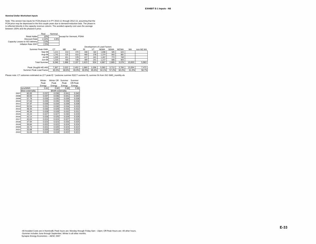
EXHIBIT E-1 Inputs - N$
Nominal Dollar Worksheet Inputs
Real NominalRetail Adder 10% except for Vermont, PSNH
Discount Rate 2.22% 4.8%Capacity Losses to ISO delivery 3.4%
Inflation Rate 2007 2.5%
Summer Peak GWh CT ME NH RI VT NEMA SEMA WCMA MA non-NE MASep-06 1,215 410 470 348 164 1,008 585 625 Aug-06 1,742 525 610 469 278 1,374 842 881 Jul-06 1,559 451 578 417 241 1,267 772 769
Jun-06 1,530 500 538 389 241 1,217 686 803 Total Summer 6,046 1,886 2,197 1,623 924 4,867 2,885 3,078 10,830 5,963
Peak 2Aug06 HE1400 7,367 2,022 2,452 1,960 1,036 5,582 3,712 3,760 13,054 7,472 Summer Peak Load Factor 60.3% 68.6% 65.9% 60.9% 65.6% 64.1% 57.2% 60.2% 61.0% 58.7%
Please note: CT subzones estimated as (CT peak lf) * (subzone summer lf)/(CT summer lf), summer lfs from ISO SMD_monthly.xls
Winter Peak
Energy
Winter Off-Peak
Energy
Summer Peak
Energy
Summer Off-Peak Energy
tons/MWh 0.61 0.60 0.68 0.66$/ton externality
2007 60.00 0.037 0.036 0.041 0.0402008 60.00 0.037 0.036 0.041 0.0402009 57.79 0.035 0.035 0.039 0.0382010 57.63 0.035 0.035 0.039 0.0382011 57.47 0.035 0.034 0.039 0.0382012 50.54 0.031 0.030 0.034 0.0332013 48.44 0.030 0.029 0.033 0.0322014 46.34 0.028 0.028 0.032 0.0312015 44.24 0.027 0.027 0.030 0.0292016 42.14 0.026 0.025 0.029 0.0282017 40.04 0.024 0.024 0.027 0.0262018 37.94 0.023 0.023 0.026 0.0252019 35.84 0.022 0.022 0.024 0.0242020 33.73 0.021 0.020 0.023 0.0222021 32.68 0.020 0.020 0.022 0.0222022 31.63 0.019 0.019 0.022 0.021
Note: This version has inputs for FCM phase-in in PY 2010-11 through 2012-13, assuming that the PCM price may be depressed in the first couple years due to demand-reduction bids. The phase-in is reflected directly in the capacity revenue column. The avoided capacity cost uses the average between 100% and the phased-in price.
$/kWh externality
Development of Load Factors
-All Avoided Costs are in Nominal$; Peak hours are: Monday through Friday 6am - 10pm; Off-Peak Hours are: All other hours.-Summer includes June through September; Winter is all other months.Synapse Energy Economics – AESC 2007
E-33
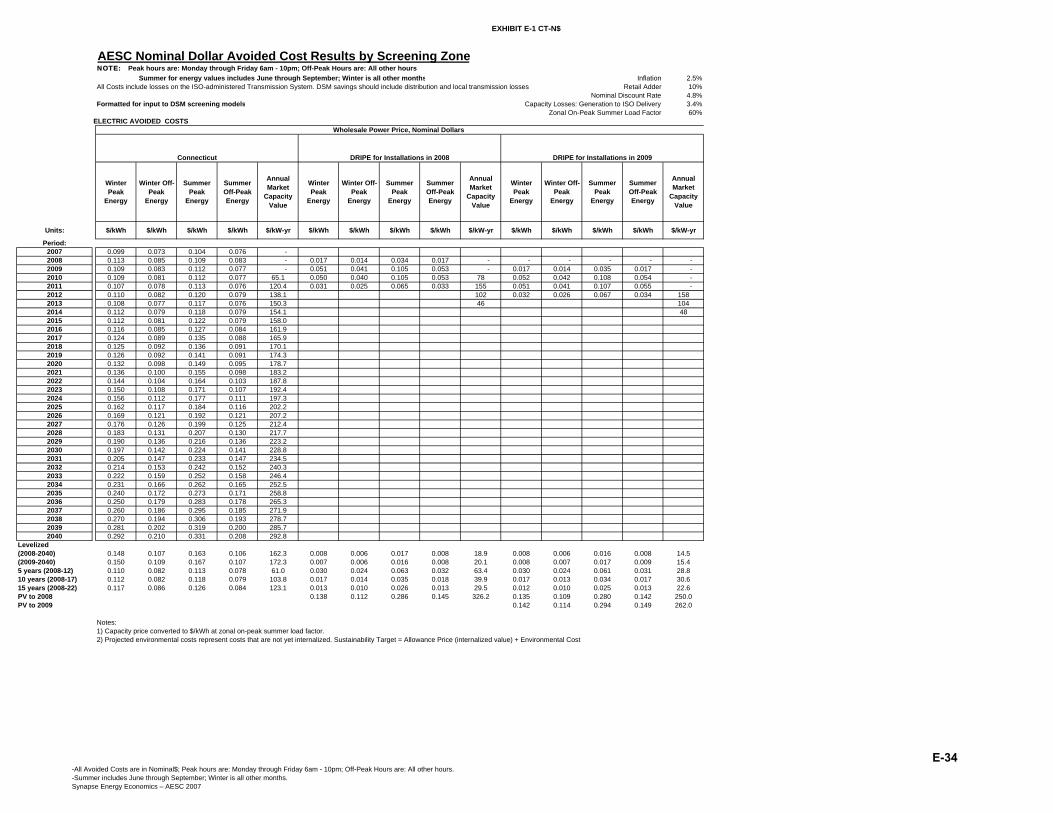
EXHIBIT E-1 CT-N$
AESC Nominal Dollar Avoided Cost Results by Screening ZoneNOTE: Peak hours are: Monday through Friday 6am - 10pm; Off-Peak Hours are: All other hours Summer for energy values includes June through September; Winter is all other months Inflation 2.5%All Costs include losses on the ISO-administered Transmission System. DSM savings should include distribution and local transmission losses Retail Adder 10%
Nominal Discount Rate 4.8%Formatted for input to DSM screening models Capacity Losses: Generation to ISO Delivery 3.4%
Zonal On-Peak Summer Load Factor 60%ELECTRIC AVOIDED COSTS
Winter Peak
Energy
Winter Off-Peak
Energy
Summer Peak
Energy
Summer Off-Peak Energy
Annual Market
Capacity Value
Winter Peak
Energy
Winter Off-Peak
Energy
Summer Peak
Energy
Summer Off-Peak Energy
Annual Market
Capacity Value
Winter Peak
Energy
Winter Off-Peak
Energy
Summer Peak
Energy
Summer Off-Peak Energy
Annual Market
Capacity Value
Units: $/kWh $/kWh $/kWh $/kWh $/kW-yr $/kWh $/kWh $/kWh $/kWh $/kW-yr $/kWh $/kWh $/kWh $/kWh $/kW-yr
Period:2007 0.099 0.073 0.104 0.076 - 2008 0.113 0.085 0.109 0.083 - 0.017 0.014 0.034 0.017 - - - - - - 2009 0.109 0.083 0.112 0.077 - 0.051 0.041 0.105 0.053 - 0.017 0.014 0.035 0.017 - 2010 0.109 0.081 0.112 0.077 65.1 0.050 0.040 0.105 0.053 78 0.052 0.042 0.108 0.054 - 2011 0.107 0.078 0.113 0.076 120.4 0.031 0.025 0.065 0.033 155 0.051 0.041 0.107 0.055 - 2012 0.110 0.082 0.120 0.079 138.1 102 0.032 0.026 0.067 0.034 1582013 0.108 0.077 0.117 0.076 150.3 46 1042014 0.112 0.079 0.118 0.079 154.1 482015 0.112 0.081 0.122 0.079 158.02016 0.116 0.085 0.127 0.084 161.92017 0.124 0.089 0.135 0.088 165.92018 0.125 0.092 0.136 0.091 170.12019 0.126 0.092 0.141 0.091 174.32020 0.132 0.098 0.149 0.095 178.72021 0.136 0.100 0.155 0.098 183.22022 0.144 0.104 0.164 0.103 187.82023 0.150 0.108 0.171 0.107 192.42024 0.156 0.112 0.177 0.111 197.32025 0.162 0.117 0.184 0.116 202.22026 0.169 0.121 0.192 0.121 207.22027 0.176 0.126 0.199 0.125 212.42028 0.183 0.131 0.207 0.130 217.72029 0.190 0.136 0.216 0.136 223.22030 0.197 0.142 0.224 0.141 228.82031 0.205 0.147 0.233 0.147 234.52032 0.214 0.153 0.242 0.152 240.32033 0.222 0.159 0.252 0.158 246.42034 0.231 0.166 0.262 0.165 252.52035 0.240 0.172 0.273 0.171 258.82036 0.250 0.179 0.283 0.178 265.32037 0.260 0.186 0.295 0.185 271.92038 0.270 0.194 0.306 0.193 278.72039 0.281 0.202 0.319 0.200 285.72040 0.292 0.210 0.331 0.208 292.8
Levelized(2008-2040) 0.148 0.107 0.163 0.106 162.3 0.008 0.006 0.017 0.008 18.9 0.008 0.006 0.016 0.008 14.5(2009-2040) 0.150 0.109 0.167 0.107 172.3 0.007 0.006 0.016 0.008 20.1 0.008 0.007 0.017 0.009 15.45 years (2008-12) 0.110 0.082 0.113 0.078 61.0 0.030 0.024 0.063 0.032 63.4 0.030 0.024 0.061 0.031 28.810 years (2008-17) 0.112 0.082 0.118 0.079 103.8 0.017 0.014 0.035 0.018 39.9 0.017 0.013 0.034 0.017 30.615 years (2008-22) 0.117 0.086 0.126 0.084 123.1 0.013 0.010 0.026 0.013 29.5 0.012 0.010 0.025 0.013 22.6PV to 2008 0.138 0.112 0.286 0.145 326.2 0.135 0.109 0.280 0.142 250.0PV to 2009 0.142 0.114 0.294 0.149 262.0
Notes: 1) Capacity price converted to $/kWh at zonal on-peak summer load factor.2) Projected environmental costs represent costs that are not yet internalized. Sustainability Target = Allowance Price (internalized value) + Environmental Cost
Wholesale Power Price, Nominal Dollars
Connecticut DRIPE for Installations in 2008 DRIPE for Installations in 2009
-All Avoided Costs are in Nominal$; Peak hours are: Monday through Friday 6am - 10pm; Off-Peak Hours are: All other hours.-Summer includes June through September; Winter is all other months.Synapse Energy Economics – AESC 2007
E-34
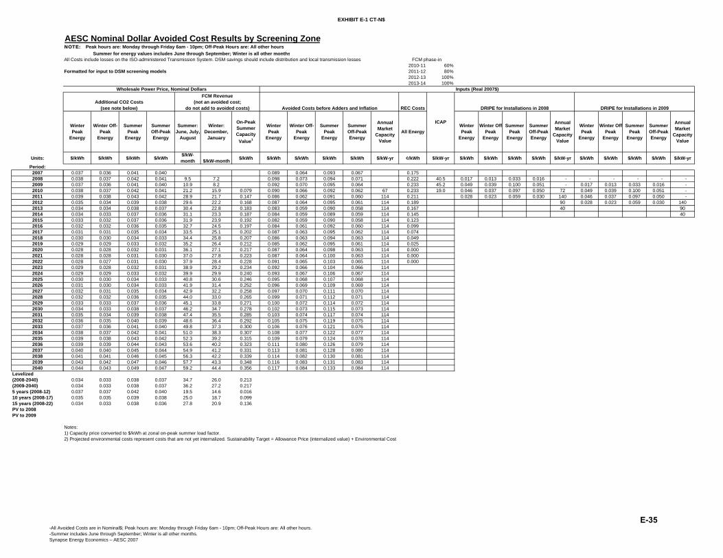
EXHIBIT E-1 CT-N$
Units:
Period:2007200820092010201120122013201420152016201720182019202020212022202320242025202620272028202920302031203220332034203520362037203820392040
Levelized(2008-2040)(2009-2040)5 years (2008-12)10 years (2008-17)15 years (2008-22)PV to 2008PV to 2009
AESC Nominal Dollar Avoided Cost Results by Screening ZoneNOTE: Peak hours are: Monday through Friday 6am - 10pm; Off-Peak Hours are: All other hours Summer for energy values includes June through September; Winter is all other monthsAll Costs include losses on the ISO-administered Transmission System. DSM savings should include distribution and local transmission losses
2010-11 60%Formatted for input to DSM screening models 2011-12 80%
2012-13 100%2013-14 100%
REC Costs
Winter Peak
Energy
Winter Off-Peak
Energy
Summer Peak
Energy
Summer Off-Peak Energy
Summer: June, July,
August
Winter: December,
January
On-Peak Summer Capacity
Value1
Winter Peak
Energy
Winter Off-Peak
Energy
Summer Peak
Energy
Summer Off-Peak Energy
Annual Market
Capacity Value
All EnergyWinter Peak
Energy
Winter OffPeak
Energy
Summer Peak
Energy
Summer Off-Peak Energy
Annual Market
Capacity Value
Winter Peak
Energy
Winter OffPeak
Energy
Summer Peak
Energy
Summer Off-Peak Energy
Annual Market
Capacity Value
$/kWh $/kWh $/kWh $/kWh$/kW-month $/kW-month $/kWh $/kWh $/kWh $/kWh $/kWh $/kW-yr ¢/kWh $/kW-yr $/kWh $/kWh $/kWh $/kWh $/kW-yr $/kWh $/kWh $/kWh $/kWh $/kW-yr
0.037 0.036 0.041 0.040 0.089 0.064 0.093 0.067 0.1750.038 0.037 0.042 0.041 9.5 7.2 0.098 0.073 0.094 0.071 0.222 40.5 0.017 0.013 0.033 0.016 - - - - - - 0.037 0.036 0.041 0.040 10.9 8.2 0.092 0.070 0.095 0.064 0.233 45.2 0.049 0.039 0.100 0.051 - 0.017 0.013 0.033 0.016 - 0.038 0.037 0.042 0.041 21.2 15.9 0.079 0.090 0.066 0.092 0.062 67 0.233 19.0 0.046 0.037 0.097 0.050 72 0.049 0.039 0.100 0.051 - 0.039 0.038 0.043 0.042 28.9 21.7 0.147 0.086 0.062 0.091 0.060 114 0.211 0.028 0.023 0.059 0.030 140 0.046 0.037 0.097 0.050 - 0.035 0.034 0.039 0.038 29.6 22.2 0.168 0.087 0.064 0.095 0.061 114 0.189 90 0.028 0.023 0.059 0.030 1400.034 0.034 0.038 0.037 30.4 22.8 0.183 0.083 0.059 0.090 0.058 114 0.167 40 900.034 0.033 0.037 0.036 31.1 23.3 0.187 0.084 0.059 0.089 0.059 114 0.145 400.033 0.032 0.037 0.036 31.9 23.9 0.192 0.082 0.059 0.090 0.058 114 0.1230.032 0.032 0.036 0.035 32.7 24.5 0.197 0.084 0.061 0.092 0.060 114 0.0990.031 0.031 0.035 0.034 33.5 25.1 0.202 0.087 0.063 0.095 0.062 114 0.0740.030 0.030 0.034 0.033 34.4 25.8 0.207 0.086 0.063 0.094 0.063 114 0.0490.029 0.029 0.033 0.032 35.2 26.4 0.212 0.085 0.062 0.095 0.061 114 0.0250.028 0.028 0.032 0.031 36.1 27.1 0.217 0.087 0.064 0.098 0.063 114 0.0000.028 0.028 0.031 0.030 37.0 27.8 0.223 0.087 0.064 0.100 0.063 114 0.0000.028 0.027 0.031 0.030 37.9 28.4 0.228 0.091 0.065 0.103 0.065 114 0.0000.029 0.028 0.032 0.031 38.9 29.2 0.234 0.092 0.066 0.104 0.066 1140.029 0.029 0.033 0.032 39.9 29.9 0.240 0.093 0.067 0.106 0.067 1140.030 0.030 0.034 0.033 40.8 30.6 0.246 0.095 0.068 0.107 0.068 1140.031 0.030 0.034 0.033 41.9 31.4 0.252 0.096 0.069 0.109 0.069 1140.032 0.031 0.035 0.034 42.9 32.2 0.258 0.097 0.070 0.111 0.070 1140.032 0.032 0.036 0.035 44.0 33.0 0.265 0.099 0.071 0.112 0.071 1140.033 0.033 0.037 0.036 45.1 33.8 0.271 0.100 0.072 0.114 0.072 1140.034 0.033 0.038 0.037 46.2 34.7 0.278 0.102 0.073 0.115 0.073 1140.035 0.034 0.039 0.038 47.4 35.5 0.285 0.103 0.074 0.117 0.074 1140.036 0.035 0.040 0.039 48.6 36.4 0.292 0.105 0.075 0.119 0.075 1140.037 0.036 0.041 0.040 49.8 37.3 0.300 0.106 0.076 0.121 0.076 1140.038 0.037 0.042 0.041 51.0 38.3 0.307 0.108 0.077 0.122 0.077 1140.039 0.038 0.043 0.042 52.3 39.2 0.315 0.109 0.079 0.124 0.078 1140.039 0.039 0.044 0.043 53.6 40.2 0.323 0.111 0.080 0.126 0.079 1140.040 0.040 0.045 0.044 54.9 41.2 0.331 0.113 0.081 0.128 0.080 1140.041 0.041 0.046 0.045 56.3 42.2 0.339 0.114 0.082 0.130 0.081 1140.043 0.042 0.047 0.046 57.7 43.3 0.348 0.116 0.083 0.131 0.083 1140.044 0.043 0.049 0.047 59.2 44.4 0.356 0.117 0.084 0.133 0.084 114
0.034 0.033 0.038 0.037 34.7 26.0 0.2130.034 0.033 0.038 0.037 36.2 27.2 0.2170.037 0.037 0.042 0.040 19.5 14.6 0.0160.035 0.035 0.039 0.038 25.0 18.7 0.0990.034 0.033 0.038 0.036 27.8 20.9 0.136
Notes: 1) Capacity price converted to $/kWh at zonal on-peak summer load factor.2) Projected environmental costs represent costs that are not yet internalized. Sustainability Target = Allowance Price (internalized value) + Environmental Cost
Wholesale Power Price, Nominal Dollars
Avoided Costs before Adders and Inflation
FCM phase-in
Additional CO2 Costs(see note below)
ICAP
Inputs (Real 2007$)
DRIPE for Installations in 2008 DRIPE for Installations in 2009
FCM Revenue(not an avoided cost;
do not add to avoided costs)
-All Avoided Costs are in Nominal$; Peak hours are: Monday through Friday 6am - 10pm; Off-Peak Hours are: All other hours.-Summer includes June through September; Winter is all other months.Synapse Energy Economics – AESC 2007
E-35
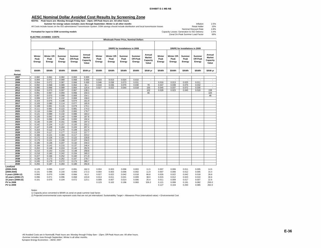
EXHIBIT E-1 ME-N$
AESC Nominal Dollar Avoided Cost Results by Screening ZoneNOTE: Peak hours are: Monday through Friday 6am - 10pm; Off-Peak Hours are: All other hours Summer for energy values includes June through September; Winter is all other months Inflation 2.5%All Costs include losses on the ISO-administered Transmission System. DSM savings should include distribution and local transmission losses Retail Adder 10%
Nominal Discount Rate 4.8%Formatted for input to DSM screening models Capacity Losses: Generation to ISO Delivery 3.4%
Zonal On-Peak Summer Load Factor 69%ELECTRIC AVOIDED COSTS
Winter Peak
Energy
Winter Off-Peak
Energy
Summer Peak
Energy
Summer Off-Peak Energy
Annual Market
Capacity Value
Winter Peak
Energy
Winter Off-Peak
Energy
Summer Peak
Energy
Summer Off-Peak Energy
Annual Market
Capacity Value
Winter Peak
Energy
Winter Off-Peak
Energy
Summer Peak
Energy
Summer Off-Peak Energy
Annual Market
Capacity Value
Units: $/kWh $/kWh $/kWh $/kWh $/kW-yr $/kWh $/kWh $/kWh $/kWh $/kW-yr $/kWh $/kWh $/kWh $/kWh $/kW-yr
Period:2007 0.082 0.061 0.082 0.063 0.0002008 0.094 0.072 0.089 0.068 0.000 0.015 0.013 0.024 0.010 - - - - - - 2009 0.094 0.072 0.087 0.066 0.000 0.046 0.038 0.073 0.031 - 0.016 0.013 0.025 0.011 - 2010 0.092 0.068 0.089 0.064 65.1 0.044 0.036 0.070 0.030 78 0.047 0.039 0.075 0.032 - 2011 0.090 0.068 0.089 0.064 120.4 0.027 0.022 0.044 0.018 155 0.045 0.037 0.072 0.030 - 2012 0.094 0.070 0.097 0.067 138.1 102 0.028 0.023 0.045 0.019 1582013 0.091 0.067 0.094 0.066 150.3 46 1042014 0.097 0.070 0.099 0.069 154.1 482015 0.099 0.072 0.102 0.069 158.02016 0.104 0.075 0.108 0.074 161.92017 0.109 0.080 0.114 0.077 165.92018 0.108 0.081 0.115 0.079 170.12019 0.111 0.081 0.122 0.081 174.32020 0.116 0.084 0.125 0.083 178.72021 0.121 0.089 0.132 0.086 183.22022 0.126 0.092 0.140 0.089 187.82023 0.131 0.096 0.146 0.093 192.42024 0.136 0.100 0.151 0.096 197.32025 0.142 0.104 0.157 0.100 202.22026 0.147 0.108 0.164 0.104 207.22027 0.153 0.112 0.170 0.108 212.42028 0.159 0.117 0.177 0.113 217.72029 0.166 0.121 0.184 0.117 223.22030 0.172 0.126 0.191 0.122 228.82031 0.179 0.131 0.199 0.127 234.52032 0.186 0.136 0.207 0.132 240.32033 0.194 0.142 0.215 0.137 246.42034 0.202 0.148 0.224 0.142 252.52035 0.210 0.153 0.233 0.148 258.82036 0.218 0.160 0.242 0.154 265.32037 0.227 0.166 0.252 0.160 271.92038 0.236 0.173 0.262 0.167 278.72039 0.245 0.179 0.272 0.173 285.72040 0.255 0.187 0.283 0.180 292.8
Levelized(2008-2040) 0.129 0.095 0.137 0.091 162.3 0.004 0.003 0.006 0.003 11.5 0.007 0.006 0.011 0.005 14.5(2009-2040) 0.131 0.096 0.140 0.093 172.3 0.004 0.003 0.006 0.002 11.9 0.007 0.006 0.012 0.005 15.45 years (2008-12) 0.093 0.070 0.090 0.066 61.0 0.027 0.022 0.042 0.018 66.8 0.026 0.022 0.042 0.018 28.810 years (2008-17) 0.096 0.071 0.096 0.068 103.8 0.013 0.011 0.021 0.009 38.0 0.015 0.012 0.023 0.010 30.615 years (2008-22) 0.101 0.075 0.104 0.072 123.1 0.009 0.007 0.014 0.006 25.4 0.011 0.009 0.017 0.007 22.6PV to 2008 0.123 0.102 0.196 0.083 326.2 0.121 0.099 0.191 0.082 250.0PV to 2009 0.127 0.104 0.200 0.085 262.0
Notes: 1) Capacity price converted to $/kWh at zonal on-peak summer load factor.2) Projected environmental costs represent costs that are not yet internalized. Sustainability Target = Allowance Price (internalized value) + Environmental Cost
Maine DRIPE for Installations in 2008 DRIPE for Installations in 2009
Wholesale Power Price, Nominal Dollars
-All Avoided Costs are in Nominal$; Peak hours are: Monday through Friday 6am - 10pm; Off-Peak Hours are: All other hours.-Summer includes June through September; Winter is all other months.Synapse Energy Economics – AESC 2007
E-36

EXHIBIT E-1 ME-N$
Units:
Period:2007200820092010201120122013201420152016201720182019202020212022202320242025202620272028202920302031203220332034203520362037203820392040
Levelized(2008-2040)(2009-2040)5 years (2008-12)10 years (2008-17)15 years (2008-22)PV to 2008PV to 2009
AESC Nominal Dollar Avoided Cost Results by Screening ZoneNOTE: Peak hours are: Monday through Friday 6am - 10pm; Off-Peak Hours are: All other hours Summer for energy values includes June through September; Winter is all other monthsAll Costs include losses on the ISO-administered Transmission System. DSM savings should include distribution and local transmission losses
2010-11 60%Formatted for input to DSM screening models 2011-12 80%
2012-13 100%2013-14 100%
REC Costs
Winter Peak
Energy
Winter Off-Peak
Energy
Summer Peak
Energy
Summer Off-Peak Energy
Summer: June, July,
August
Winter: December,
January
On-Peak Summer Capacity
Value1
Winter Peak
Energy
Winter Off-Peak
Energy
Summer Peak
Energy
Summer Off-Peak Energy
Annual Market
Capacity Value
All EnergyWinter Peak
Energy
Winter OffPeak
Energy
Summer Peak
Energy
Summer Off-Peak Energy
Annual Market
Capacity Value
Winter Peak
Energy
Winter OffPeak
Energy
Summer Peak
Energy
Summer Off-Peak Energy
Annual Market
Capacity Value
$/kWh $/kWh $/kWh $/kWh$/kW-month $/kW-month $/kWh $/kWh $/kWh $/kWh $/kWh $/kW-yr ¢/kWh $/kW-yr $/kWh $/kWh $/kWh $/kWh $/kW-yr $/kWh $/kWh $/kWh $/kWh $/kW-yr
0.037 0.036 0.041 0.040 0.075 0.056 0.074 0.058 0.0000.038 0.037 0.042 0.041 9.5 7.2 0.083 0.064 0.078 0.060 0.044 40.5 0.015 0.012 0.024 0.010 - - - - - - 0.037 0.036 0.041 0.040 10.9 8.2 0.080 0.061 0.075 0.057 0.078 45.2 0.044 0.037 0.069 0.030 - 0.015 0.012 0.024 0.010 - 0.038 0.037 0.042 0.041 21.2 15.9 0.070 0.076 0.057 0.074 0.053 67 0.100 19.0 0.041 0.034 0.065 0.028 72 0.044 0.037 0.069 0.030 - 0.039 0.038 0.043 0.042 28.9 21.7 0.129 0.073 0.055 0.072 0.051 114 0.121 0.025 0.020 0.040 0.017 140 0.041 0.034 0.065 0.028 - 0.035 0.034 0.039 0.038 29.6 22.2 0.148 0.074 0.055 0.076 0.053 114 0.135 90 0.025 0.020 0.040 0.017 1400.034 0.034 0.038 0.037 30.4 22.8 0.161 0.070 0.051 0.072 0.050 114 0.143 40 900.034 0.033 0.037 0.036 31.1 23.3 0.165 0.073 0.052 0.074 0.052 114 0.145 400.033 0.032 0.037 0.036 31.9 23.9 0.169 0.072 0.052 0.075 0.050 114 0.1410.032 0.032 0.036 0.035 32.7 24.5 0.173 0.074 0.053 0.077 0.053 114 0.1270.031 0.031 0.035 0.034 33.5 25.1 0.178 0.076 0.056 0.080 0.054 114 0.1060.030 0.030 0.034 0.033 34.4 25.8 0.182 0.074 0.055 0.079 0.054 114 0.0710.029 0.029 0.033 0.032 35.2 26.4 0.187 0.075 0.054 0.082 0.054 114 0.0350.028 0.028 0.032 0.031 36.1 27.1 0.191 0.076 0.056 0.082 0.055 114 0.0000.028 0.028 0.031 0.030 37.0 27.8 0.196 0.078 0.057 0.085 0.055 114 0.0000.028 0.027 0.031 0.030 37.9 28.4 0.201 0.079 0.058 0.088 0.056 114 0.0000.029 0.028 0.032 0.031 38.9 29.2 0.206 0.080 0.059 0.089 0.057 1140.029 0.029 0.033 0.032 39.9 29.9 0.211 0.081 0.060 0.090 0.058 1140.030 0.030 0.034 0.033 40.8 30.6 0.216 0.083 0.061 0.092 0.058 1140.031 0.030 0.034 0.033 41.9 31.4 0.222 0.084 0.061 0.093 0.059 1140.032 0.031 0.035 0.034 42.9 32.2 0.227 0.085 0.062 0.094 0.060 1140.032 0.032 0.036 0.035 44.0 33.0 0.233 0.086 0.063 0.096 0.061 1140.033 0.033 0.037 0.036 45.1 33.8 0.239 0.088 0.064 0.097 0.062 1140.034 0.033 0.038 0.037 46.2 34.7 0.245 0.089 0.065 0.099 0.063 1140.035 0.034 0.039 0.038 47.4 35.5 0.251 0.090 0.066 0.100 0.064 1140.036 0.035 0.040 0.039 48.6 36.4 0.257 0.091 0.067 0.102 0.065 1140.037 0.036 0.041 0.040 49.8 37.3 0.264 0.093 0.068 0.103 0.066 1140.038 0.037 0.042 0.041 51.0 38.3 0.270 0.094 0.069 0.104 0.067 1140.039 0.038 0.043 0.042 52.3 39.2 0.277 0.095 0.070 0.106 0.067 1140.039 0.039 0.044 0.043 53.6 40.2 0.284 0.097 0.071 0.108 0.068 1140.040 0.040 0.045 0.044 54.9 41.2 0.291 0.098 0.072 0.109 0.069 1140.041 0.041 0.046 0.045 56.3 42.2 0.298 0.100 0.073 0.111 0.070 1140.043 0.042 0.047 0.046 57.7 43.3 0.306 0.101 0.074 0.112 0.071 1140.044 0.043 0.049 0.047 59.2 44.4 0.313 0.103 0.075 0.114 0.073 114
0.034 0.034 0.038 0.037 39.7 29.8 0.1880.034 0.034 0.038 0.037 40.7 30.5 0.1910.037 0.037 0.041 0.040 20.0 15.0 0.0150.035 0.034 0.039 0.038 26.0 19.5 0.0870.033 0.032 0.037 0.036 29.4 22.0 0.120
Notes: 1) Capacity price converted to $/kWh at zonal on-peak summer load factor.2) Projected environmental costs represent costs that are not yet internalized. Sustainability Target = Allowance Price (internalized value) + Environmental Cost
DRIPE for Installations in 2008 DRIPE for Installations in 2009
FCM Revenue(not an avoided cost;
do not add to avoided costs)
Wholesale Power Price, Nominal Dollars
FCM phase-in
Avoided Costs before Adders and InflationAdditional CO2 Costs
(see note below)
Inputs (Real 2007$)
ICAP
-All Avoided Costs are in Nominal$; Peak hours are: Monday through Friday 6am - 10pm; Off-Peak Hours are: All other hours.-Summer includes June through September; Winter is all other months.Synapse Energy Economics – AESC 2007
E-37

EXHIBIT E-1 MA-N$
AESC Nominal Dollar Avoided Cost Results by Screening ZoneNOTE: Peak hours are: Monday through Friday 6am - 10pm; Off-Peak Hours are: All other hours Summer for energy values includes June through September; Winter is all other months Inflation 2.5%All Costs include losses on the ISO-administered Transmission System. DSM savings should include distribution and local transmission losses Retail Adder 10%
Nominal Discount Rate 4.8%Formatted for input to DSM screening models Capacity Losses: Generation to ISO Delivery 3.4%
Zonal On-Peak Summer Load Factor 61%ELECTRIC AVOIDED COSTS
Winter Peak
Energy
Winter Off-Peak
Energy
Summer Peak
Energy
Summer Off-Peak Energy
Annual Market
Capacity Value
Winter Peak
Energy
Winter Off-Peak
Energy
Summer Peak
Energy
Summer Off-Peak Energy
Annual Market
Capacity Value
Winter Peak
Energy
Winter Off-Peak
Energy
Summer Peak
Energy
Summer Off-Peak Energy
Annual Market
Capacity Value
Units: $/kWh $/kWh $/kWh $/kWh $/kW-yr $/kWh $/kWh $/kWh $/kWh $/kW-yr $/kWh $/kWh $/kWh $/kWh $/kW-yr
Period:2007 0.094 0.069 0.095 0.072 - 2008 0.108 0.080 0.100 0.076 - 0.016 0.013 0.029 0.012 - - - - - - 2009 0.103 0.079 0.102 0.074 - 0.049 0.039 0.088 0.036 - 0.017 0.014 0.030 0.012 - 2010 0.105 0.077 0.106 0.072 65.1 0.046 0.037 0.084 0.034 78 0.050 0.040 0.090 0.037 - 2011 0.103 0.076 0.107 0.072 120.4 0.029 0.023 0.052 0.021 155 0.047 0.038 0.086 0.035 - 2012 0.106 0.079 0.111 0.077 138.1 102 0.030 0.024 0.053 0.022 1582013 0.103 0.075 0.109 0.075 150.3 46 1042014 0.108 0.077 0.112 0.078 154.1 482015 0.109 0.080 0.120 0.079 158.02016 0.115 0.083 0.124 0.085 161.92017 0.121 0.087 0.130 0.086 165.92018 0.121 0.089 0.132 0.089 170.12019 0.123 0.089 0.138 0.089 174.32020 0.128 0.094 0.142 0.092 178.72021 0.133 0.097 0.152 0.096 183.22022 0.141 0.101 0.158 0.100 187.82023 0.146 0.105 0.165 0.104 192.42024 0.152 0.109 0.171 0.108 197.32025 0.158 0.113 0.178 0.113 202.22026 0.164 0.118 0.185 0.117 207.22027 0.171 0.122 0.193 0.122 212.42028 0.178 0.127 0.200 0.127 217.72029 0.185 0.132 0.208 0.132 223.22030 0.192 0.138 0.216 0.137 228.82031 0.200 0.143 0.225 0.142 234.52032 0.208 0.149 0.234 0.148 240.32033 0.216 0.155 0.243 0.154 246.42034 0.225 0.161 0.253 0.160 252.52035 0.234 0.167 0.263 0.167 258.82036 0.243 0.174 0.274 0.173 265.32037 0.253 0.181 0.285 0.180 271.92038 0.263 0.188 0.296 0.187 278.72039 0.273 0.196 0.308 0.195 285.72040 0.284 0.204 0.320 0.203 292.8
Levelized(2008-2040) 0.144 0.104 0.157 0.103 162.3 0.008 0.006 0.014 0.006 18.9 0.007 0.006 0.013 0.005 14.5(2009-2040) 0.146 0.106 0.160 0.104 172.3 0.007 0.006 0.013 0.005 20.1 0.008 0.006 0.014 0.006 15.45 years (2008-12) 0.105 0.078 0.105 0.074 61.0 0.028 0.023 0.051 0.021 63.4 0.028 0.022 0.050 0.020 28.810 years (2008-17) 0.108 0.079 0.111 0.077 103.8 0.016 0.013 0.029 0.012 39.9 0.016 0.013 0.028 0.011 30.615 years (2008-22) 0.113 0.083 0.119 0.081 123.1 0.012 0.010 0.021 0.009 29.5 0.012 0.009 0.021 0.008 22.6PV to 2008 0.130 0.105 0.234 0.095 326.2 0.127 0.103 0.229 0.093 250.0PV to 2009 0.133 0.108 0.240 0.097 262.0
Notes: 1) Capacity price converted to $/kWh at zonal on-peak summer load factor.2) Projected environmental costs represent costs that are not yet internalized. Sustainability Target = Allowance Price (internalized value) + Environmental Cost
All of Massachusetts DRIPE for Installations in 2008 DRIPE for Installations in 2009
Wholesale Power Price, Nominal Dollars
-All Avoided Costs are in Nominal$; Peak hours are: Monday through Friday 6am - 10pm; Off-Peak Hours are: All other hours.-Summer includes June through September; Winter is all other months.Synapse Energy Economics – AESC 2007
E-38
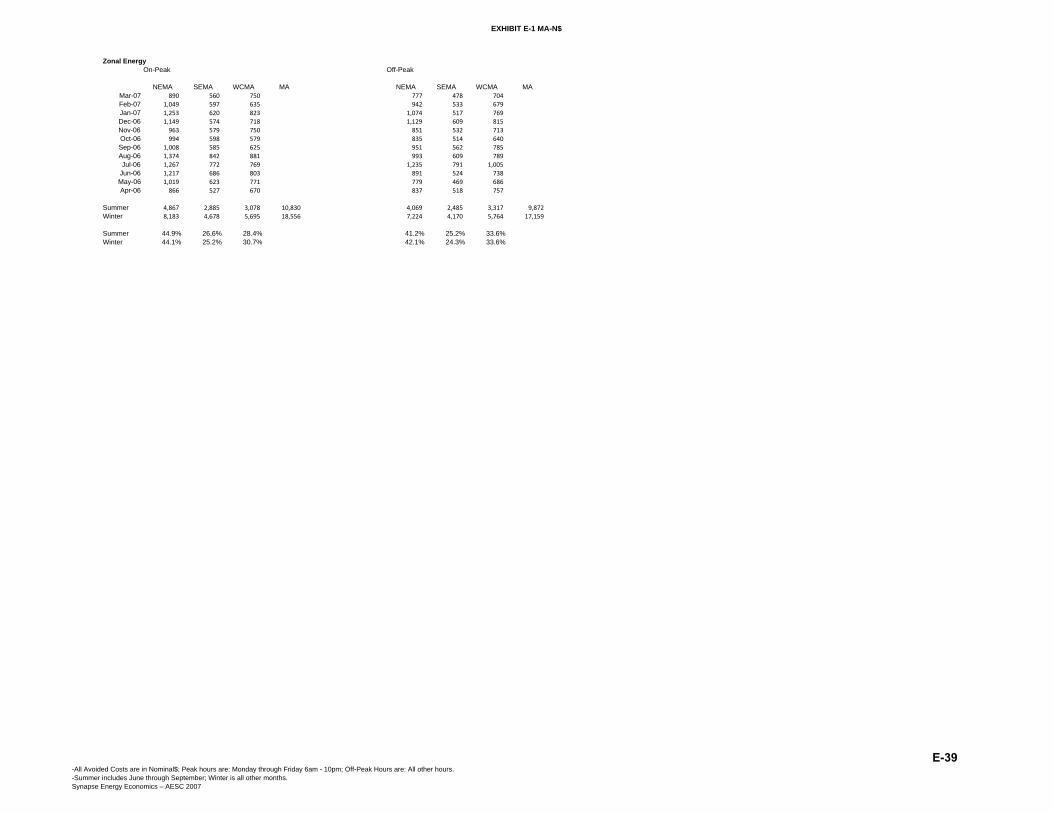
EXHIBIT E-1 MA-N$
Zonal EnergyOn-Peak Off-Peak
NEMA SEMA WCMA MA NEMA SEMA WCMA MAMar-07 890 560 750 777 478 704 Feb-07 1,049 597 635 942 533 679 Jan-07 1,253 620 823 1,074 517 769 Dec-06 1,149 574 718 1,129 609 815 Nov-06 963 579 750 851 532 713 Oct-06 994 598 579 835 514 640 Sep-06 1,008 585 625 951 562 785 Aug-06 1,374 842 881 993 609 789 Jul-06 1,267 772 769 1,235 791 1,005
Jun-06 1,217 686 803 891 524 738 May-06 1,019 623 771 779 469 686 Apr-06 866 527 670 837 518 757
Summer 4,867 2,885 3,078 10,830 4,069 2,485 3,317 9,872 Winter 8,183 4,678 5,695 18,556 7,224 4,170 5,764 17,159
Summer 44.9% 26.6% 28.4% 41.2% 25.2% 33.6%Winter 44.1% 25.2% 30.7% 42.1% 24.3% 33.6%
-All Avoided Costs are in Nominal$; Peak hours are: Monday through Friday 6am - 10pm; Off-Peak Hours are: All other hours.-Summer includes June through September; Winter is all other months.Synapse Energy Economics – AESC 2007
E-39
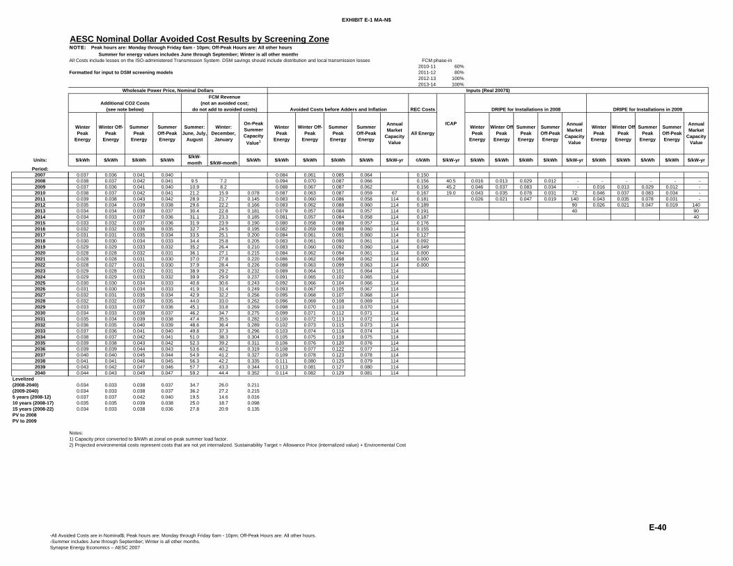
EXHIBIT E-1 MA-N$
Units:
Period:2007200820092010201120122013201420152016201720182019202020212022202320242025202620272028202920302031203220332034203520362037203820392040
Levelized(2008-2040)(2009-2040)5 years (2008-12)10 years (2008-17)15 years (2008-22)PV to 2008PV to 2009
AESC Nominal Dollar Avoided Cost Results by Screening ZoneNOTE: Peak hours are: Monday through Friday 6am - 10pm; Off-Peak Hours are: All other hours Summer for energy values includes June through September; Winter is all other monthsAll Costs include losses on the ISO-administered Transmission System. DSM savings should include distribution and local transmission losses
2010-11 60%Formatted for input to DSM screening models 2011-12 80%
2012-13 100%2013-14 100%
REC Costs
Winter Peak
Energy
Winter Off-Peak
Energy
Summer Peak
Energy
Summer Off-Peak Energy
Summer: June, July,
August
Winter: December,
January
On-Peak Summer Capacity
Value1
Winter Peak
Energy
Winter Off-Peak
Energy
Summer Peak
Energy
Summer Off-Peak Energy
Annual Market
Capacity Value
All EnergyWinter Peak
Energy
Winter OffPeak
Energy
Summer Peak
Energy
Summer Off-Peak Energy
Annual Market
Capacity Value
Winter Peak
Energy
Winter OffPeak
Energy
Summer Peak
Energy
Summer Off-Peak Energy
Annual Market
Capacity Value
$/kWh $/kWh $/kWh $/kWh$/kW-month $/kW-month $/kWh $/kWh $/kWh $/kWh $/kWh $/kW-yr ¢/kWh $/kW-yr $/kWh $/kWh $/kWh $/kWh $/kW-yr $/kWh $/kWh $/kWh $/kWh $/kW-yr
0.037 0.036 0.041 0.040 0.084 0.061 0.085 0.064 0.1500.038 0.037 0.042 0.041 9.5 7.2 0.094 0.070 0.087 0.066 0.156 40.5 0.016 0.013 0.029 0.012 - - - - - - 0.037 0.036 0.041 0.040 10.9 8.2 0.088 0.067 0.087 0.062 0.156 45.2 0.046 0.037 0.083 0.034 - 0.016 0.013 0.029 0.012 - 0.038 0.037 0.042 0.041 21.2 15.9 0.078 0.087 0.063 0.087 0.059 67 0.167 19.0 0.043 0.035 0.078 0.031 72 0.046 0.037 0.083 0.034 - 0.039 0.038 0.043 0.042 28.9 21.7 0.145 0.083 0.060 0.086 0.058 114 0.181 0.026 0.021 0.047 0.019 140 0.043 0.035 0.078 0.031 - 0.035 0.034 0.039 0.038 29.6 22.2 0.166 0.083 0.062 0.088 0.060 114 0.189 90 0.026 0.021 0.047 0.019 1400.034 0.034 0.038 0.037 30.4 22.8 0.181 0.079 0.057 0.084 0.057 114 0.191 40 900.034 0.033 0.037 0.036 31.1 23.3 0.185 0.081 0.057 0.084 0.058 114 0.187 400.033 0.032 0.037 0.036 31.9 23.9 0.190 0.080 0.058 0.088 0.057 114 0.1760.032 0.032 0.036 0.035 32.7 24.5 0.195 0.082 0.059 0.088 0.060 114 0.1550.031 0.031 0.035 0.034 33.5 25.1 0.200 0.084 0.061 0.091 0.060 114 0.1270.030 0.030 0.034 0.033 34.4 25.8 0.205 0.083 0.061 0.090 0.061 114 0.0920.029 0.029 0.033 0.032 35.2 26.4 0.210 0.083 0.060 0.092 0.060 114 0.0490.028 0.028 0.032 0.031 36.1 27.1 0.215 0.084 0.062 0.094 0.061 114 0.0000.028 0.028 0.031 0.030 37.0 27.8 0.220 0.086 0.062 0.098 0.062 114 0.0000.028 0.027 0.031 0.030 37.9 28.4 0.226 0.088 0.063 0.099 0.063 114 0.0000.029 0.028 0.032 0.031 38.9 29.2 0.232 0.089 0.064 0.101 0.064 1140.029 0.029 0.033 0.032 39.9 29.9 0.237 0.091 0.065 0.102 0.065 1140.030 0.030 0.034 0.033 40.8 30.6 0.243 0.092 0.066 0.104 0.066 1140.031 0.030 0.034 0.033 41.9 31.4 0.249 0.093 0.067 0.105 0.067 1140.032 0.031 0.035 0.034 42.9 32.2 0.256 0.095 0.068 0.107 0.068 1140.032 0.032 0.036 0.035 44.0 33.0 0.262 0.096 0.069 0.108 0.069 1140.033 0.033 0.037 0.036 45.1 33.8 0.269 0.098 0.070 0.110 0.070 1140.034 0.033 0.038 0.037 46.2 34.7 0.275 0.099 0.071 0.112 0.071 1140.035 0.034 0.039 0.038 47.4 35.5 0.282 0.100 0.072 0.113 0.072 1140.036 0.035 0.040 0.039 48.6 36.4 0.289 0.102 0.073 0.115 0.073 1140.037 0.036 0.041 0.040 49.8 37.3 0.296 0.103 0.074 0.116 0.074 1140.038 0.037 0.042 0.041 51.0 38.3 0.304 0.105 0.075 0.118 0.075 1140.039 0.038 0.043 0.042 52.3 39.2 0.311 0.106 0.076 0.120 0.076 1140.039 0.039 0.044 0.043 53.6 40.2 0.319 0.108 0.077 0.122 0.077 1140.040 0.040 0.045 0.044 54.9 41.2 0.327 0.109 0.078 0.123 0.078 1140.041 0.041 0.046 0.045 56.3 42.2 0.335 0.111 0.080 0.125 0.079 1140.043 0.042 0.047 0.046 57.7 43.3 0.344 0.113 0.081 0.127 0.080 1140.044 0.043 0.049 0.047 59.2 44.4 0.352 0.114 0.082 0.129 0.081 114
0.034 0.033 0.038 0.037 34.7 26.0 0.2110.034 0.033 0.038 0.037 36.2 27.2 0.2150.037 0.037 0.042 0.040 19.5 14.6 0.0160.035 0.035 0.039 0.038 25.0 18.7 0.0980.034 0.033 0.038 0.036 27.8 20.9 0.135
Notes: 1) Capacity price converted to $/kWh at zonal on-peak summer load factor.2) Projected environmental costs represent costs that are not yet internalized. Sustainability Target = Allowance Price (internalized value) + Environmental Cost
DRIPE for Installations in 2008 DRIPE for Installations in 2009
ICAP
Inputs (Real 2007$)Wholesale Power Price, Nominal Dollars
FCM phase-in
Avoided Costs before Adders and InflationAdditional CO2 Costs
(see note below)
FCM Revenue(not an avoided cost;
do not add to avoided costs)
-All Avoided Costs are in Nominal$; Peak hours are: Monday through Friday 6am - 10pm; Off-Peak Hours are: All other hours.-Summer includes June through September; Winter is all other months.Synapse Energy Economics – AESC 2007
E-40

EXHIBIT E-1 NH-N$
AESC Nominal Dollar Avoided Cost Results by Screening ZoneNOTE: Peak hours are: Monday through Friday 6am - 10pm; Off-Peak Hours are: All other hours Summer for energy values includes June through September; Winter is all other months Inflation 2.5%All Costs include losses on the ISO-administered Transmission System. DSM savings should include distribution and local transmission losses Retail Adder 10%
Nominal Discount Rate 4.8%Formatted for input to DSM screening models Capacity Losses: Generation to ISO Delivery 3.4%
Zonal On-Peak Summer Load Factor 66%ELECTRIC AVOIDED COSTS
Winter Peak
Energy
Winter Off-Peak
Energy
Summer Peak
Energy
Summer Off-Peak Energy
Annual Market
Capacity Value
Winter Peak
Energy
Winter Off-Peak
Energy
Summer Peak
Energy
Summer Off-Peak Energy
Annual Market
Capacity Value
Winter Peak
Energy
Winter Off-Peak
Energy
Summer Peak
Energy
Summer Off-Peak Energy
Annual Market
Capacity Value
Units: $/kWh $/kWh $/kWh $/kWh $/kW-yr $/kWh $/kWh $/kWh $/kWh $/kW-yr $/kWh $/kWh $/kWh $/kWh $/kW-yr
Period:2007 0.089 0.066 0.090 0.0692008 0.102 0.077 0.094 0.072 0.016 0.015 0.029 0.015 - - - - - - 2009 0.098 0.076 0.094 0.070 0.044 0.039 0.079 0.036 - 0.016 0.015 0.030 0.015 - 2010 0.099 0.073 0.097 0.069 65.1 0.042 0.036 0.075 0.032 78 0.046 0.040 0.081 0.037 - 2011 0.097 0.073 0.097 0.068 120.4 0.026 0.022 0.046 0.020 155 0.043 0.037 0.077 0.033 - 2012 0.101 0.076 0.105 0.073 138.1 102 0.027 0.023 0.047 0.020 1582013 0.099 0.072 0.103 0.071 150.3 46 1042014 0.104 0.075 0.107 0.074 154.1 482015 0.105 0.077 0.111 0.075 158.02016 0.110 0.080 0.117 0.081 161.92017 0.116 0.085 0.124 0.083 165.92018 0.116 0.087 0.123 0.086 170.12019 0.119 0.087 0.130 0.087 174.32020 0.123 0.091 0.135 0.090 178.72021 0.128 0.094 0.142 0.092 183.22022 0.133 0.098 0.150 0.096 187.82023 0.139 0.102 0.156 0.100 192.42024 0.144 0.106 0.162 0.104 197.32025 0.150 0.111 0.168 0.108 202.22026 0.156 0.115 0.175 0.112 207.22027 0.162 0.120 0.182 0.117 212.42028 0.169 0.124 0.189 0.121 217.72029 0.176 0.129 0.197 0.126 223.22030 0.183 0.135 0.205 0.131 228.82031 0.190 0.140 0.213 0.136 234.52032 0.197 0.145 0.221 0.142 240.32033 0.205 0.151 0.230 0.147 246.42034 0.213 0.157 0.239 0.153 252.52035 0.222 0.164 0.249 0.159 258.82036 0.231 0.170 0.259 0.166 265.32037 0.240 0.177 0.269 0.172 271.92038 0.250 0.184 0.280 0.179 278.72039 0.259 0.191 0.291 0.186 285.72040 0.270 0.199 0.303 0.194 292.8
Levelized(2008-2040) 0.137 0.101 0.147 0.098 178.1 0.004 0.003 0.007 0.003 11.5 0.007 0.006 0.012 0.005 14.5(2009-2040) 0.139 0.103 0.151 0.100 180.5 0.004 0.003 0.006 0.003 11.9 0.007 0.006 0.013 0.006 15.45 years (2008-12) 0.099 0.075 0.097 0.070 67.0 0.026 0.022 0.046 0.021 66.8 0.026 0.022 0.046 0.020 28.810 years (2008-17) 0.102 0.076 0.104 0.073 113.9 0.013 0.011 0.023 0.010 38.0 0.014 0.012 0.025 0.011 30.615 years (2008-22) 0.108 0.080 0.112 0.077 135.2 0.009 0.007 0.015 0.007 25.4 0.011 0.009 0.019 0.008 22.6PV to 2008 0.119 0.104 0.213 0.096 326.2 0.117 0.102 0.208 0.093 250.0PV to 2009 0.122 0.107 0.218 0.098 262.0
Notes: 1) Capacity price converted to $/kWh at zonal on-peak summer load factor.2) Projected environmental costs represent costs that are not yet internalized. Sustainability Target = Allowance Price (internalized value) + Environmental Cost
New Hampshire DRIPE for Installations in 2008 DRIPE for Installations in 2009
Wholesale Power Price, Nominal Dollars
-All Avoided Costs are in Nominal$; Peak hours are: Monday through Friday 6am - 10pm; Off-Peak Hours are: All other hours.-Summer includes June through September; Winter is all other months.Synapse Energy Economics – AESC 2007
E-41

EXHIBIT E-1 NH-N$
Units:
Period:2007200820092010201120122013201420152016201720182019202020212022202320242025202620272028202920302031203220332034203520362037203820392040
Levelized(2008-2040)(2009-2040)5 years (2008-12)10 years (2008-17)15 years (2008-22)PV to 2008PV to 2009
AESC Nominal Dollar Avoided Cost Results by Screening ZoneNOTE: Peak hours are: Monday through Friday 6am - 10pm; Off-Peak Hours are: All other hours Summer for energy values includes June through September; Winter is all other monthsAll Costs include losses on the ISO-administered Transmission System. DSM savings should include distribution and local transmission losses
2010-11 60%Formatted for input to DSM screening models 2011-12 80%
2012-13 100%2013-14 100%
REC Costs
Winter Peak
Energy
Winter Off-Peak
Energy
Summer Peak
Energy
Summer Off-Peak Energy
Summer: June, July,
August
Winter: December,
January
On-Peak Summer Capacity
Value1
Winter Peak
Energy
Winter Off-Peak
Energy
Summer Peak
Energy
Summer Off-Peak Energy
Annual Market
Capacity Value
All EnergyWinter Peak
Energy
Winter OffPeak
Energy
Summer Peak
Energy
Summer Off-Peak Energy
Annual Market
Capacity Value
Winter Peak
Energy
Winter OffPeak
Energy
Summer Peak
Energy
Summer Off-Peak Energy
Annual Market
Capacity Value
$/kWh $/kWh $/kWh $/kWh$/kW-month $/kW-month $/kWh $/kWh $/kWh $/kWh $/kWh $/kW-yr ¢/kWh $/kW-yr $/kWh $/kWh $/kWh $/kWh $/kW-yr $/kWh $/kWh $/kWh $/kWh $/kW-yr
0.037 0.036 0.041 0.040 0.081 0.060 0.081 0.063 0.0000.038 0.037 0.042 0.041 9.5 7.2 0.090 0.068 0.084 0.064 0.000 40.5 0.015 0.014 0.028 0.014 - - - - - - 0.037 0.036 0.041 0.040 10.9 8.2 0.085 0.066 0.081 0.060 0.019 45.2 0.042 0.037 0.076 0.034 - 0.015 0.014 0.028 0.014 - 0.038 0.037 0.042 0.041 21.2 15.9 0.073 0.083 0.062 0.081 0.058 67 0.035 19.0 0.039 0.034 0.069 0.030 72 0.042 0.037 0.076 0.034 - 0.039 0.038 0.043 0.042 28.9 21.7 0.134 0.079 0.059 0.080 0.056 114 0.063 0.024 0.020 0.042 0.018 140 0.039 0.034 0.069 0.030 - 0.035 0.034 0.039 0.038 29.6 22.2 0.154 0.080 0.060 0.083 0.057 114 0.085 90 0.024 0.020 0.042 0.018 1400.034 0.034 0.038 0.037 30.4 22.8 0.168 0.076 0.055 0.079 0.054 114 0.100 40 900.034 0.033 0.037 0.036 31.1 23.3 0.172 0.078 0.056 0.081 0.056 114 0.110 400.033 0.032 0.037 0.036 31.9 23.9 0.176 0.077 0.056 0.082 0.055 114 0.1110.032 0.032 0.036 0.035 32.7 24.5 0.180 0.079 0.057 0.084 0.058 114 0.1030.031 0.031 0.035 0.034 33.5 25.1 0.185 0.082 0.060 0.087 0.058 114 0.0880.030 0.030 0.034 0.033 34.4 25.8 0.190 0.080 0.059 0.085 0.059 114 0.0660.029 0.029 0.033 0.032 35.2 26.4 0.194 0.080 0.058 0.088 0.058 114 0.0360.028 0.028 0.032 0.031 36.1 27.1 0.199 0.081 0.060 0.089 0.059 114 0.0000.028 0.028 0.031 0.030 37.0 27.8 0.204 0.082 0.061 0.091 0.059 114 0.0000.028 0.027 0.031 0.030 37.9 28.4 0.209 0.084 0.062 0.094 0.060 114 0.0000.029 0.028 0.032 0.031 38.9 29.2 0.214 0.085 0.063 0.095 0.061 1140.029 0.029 0.033 0.032 39.9 29.9 0.220 0.086 0.064 0.097 0.062 1140.030 0.030 0.034 0.033 40.8 30.6 0.225 0.087 0.065 0.098 0.063 1140.031 0.030 0.034 0.033 41.9 31.4 0.231 0.089 0.065 0.100 0.064 1140.032 0.031 0.035 0.034 42.9 32.2 0.237 0.090 0.066 0.101 0.065 1140.032 0.032 0.036 0.035 44.0 33.0 0.243 0.091 0.067 0.102 0.066 1140.033 0.033 0.037 0.036 45.1 33.8 0.249 0.093 0.068 0.104 0.067 1140.034 0.033 0.038 0.037 46.2 34.7 0.255 0.094 0.069 0.105 0.068 1140.035 0.034 0.039 0.038 47.4 35.5 0.261 0.095 0.070 0.107 0.069 1140.036 0.035 0.040 0.039 48.6 36.4 0.268 0.097 0.071 0.109 0.070 1140.037 0.036 0.041 0.040 49.8 37.3 0.275 0.098 0.072 0.110 0.071 1140.038 0.037 0.042 0.041 51.0 38.3 0.281 0.100 0.073 0.112 0.072 1140.039 0.038 0.043 0.042 52.3 39.2 0.288 0.101 0.074 0.113 0.073 1140.039 0.039 0.044 0.043 53.6 40.2 0.296 0.103 0.076 0.115 0.074 1140.040 0.040 0.045 0.044 54.9 41.2 0.303 0.104 0.077 0.117 0.075 1140.041 0.041 0.046 0.045 56.3 42.2 0.311 0.105 0.078 0.118 0.076 1140.043 0.042 0.047 0.046 57.7 43.3 0.318 0.107 0.079 0.120 0.077 1140.044 0.043 0.049 0.047 59.2 44.4 0.326 0.109 0.080 0.122 0.078 114
0.034 0.034 0.038 0.037 39.7 29.8 0.1950.034 0.034 0.038 0.037 40.7 30.5 0.1990.037 0.037 0.041 0.040 20.0 15.0 0.0150.035 0.034 0.039 0.038 26.0 19.5 0.0900.033 0.032 0.037 0.036 29.4 22.0 0.125
Notes: 1) Capacity price converted to $/kWh at zonal on-peak summer load factor.2) Projected environmental costs represent costs that are not yet internalized. Sustainability Target = Allowance Price (internalized value) + Environmental Cost
DRIPE for Installations in 2008 DRIPE for Installations in 2009
Inputs (Real 2007$)
ICAP
FCM phase-in
Avoided Costs before Adders and inflationAdditional CO2 Costs
(see note below)
FCM Revenue(not an avoided cost;
do not add to avoided costs)
Wholesale Power Price, Nominal Dollars
-All Avoided Costs are in Nominal$; Peak hours are: Monday through Friday 6am - 10pm; Off-Peak Hours are: All other hours.-Summer includes June through September; Winter is all other months.Synapse Energy Economics – AESC 2007
E-42

EXHIBIT E-1 RI-N$
AESC Nominal Dollar Avoided Cost Results by Screening ZoneNOTE: Peak hours are: Monday through Friday 6am - 10pm; Off-Peak Hours are: All other hours Summer for energy values includes June through September; Winter is all other months Inflation 2.5%All Costs include losses on the ISO-administered Transmission System. DSM savings should include distribution and local transmission losses Retail Adder 10%
Nominal Discount Rate 4.8%Formatted for input to DSM screening models Capacity Losses: Generation to ISO Delivery 3.4%
Zonal On-Peak Summer Load Factor 61%ELECTRIC AVOIDED COSTS
Winter Peak
Energy
Winter Off-Peak
Energy
Summer Peak
Energy
Summer Off-Peak Energy
Annual Market
Capacity Value
Winter Peak
Energy
Winter Off-Peak
Energy
Summer Peak
Energy
Summer Off-Peak Energy
Annual Market
Capacity Value
Winter Peak
Energy
Winter Off-Peak
Energy
Summer Peak
Energy
Summer Off-Peak Energy
Annual Market
Capacity Value
Units: $/kWh $/kWh $/kWh $/kWh $/kW-yr $/kWh $/kWh $/kWh $/kWh $/kW-yr $/kWh $/kWh $/kWh $/kWh $/kW-yr
Period:2007 0.092 0.067 0.093 0.070 - 2008 0.108 0.079 0.098 0.074 - 0.015 0.012 0.025 0.011 - - - - - - 2009 0.101 0.077 0.102 0.071 - 0.045 0.036 0.074 0.033 - 0.015 0.012 0.025 0.011 - 2010 0.103 0.076 0.104 0.070 65.1 0.043 0.035 0.071 0.032 78 0.046 0.037 0.076 0.034 - 2011 0.101 0.074 0.105 0.069 120.4 0.027 0.022 0.044 0.020 155 0.044 0.036 0.073 0.033 - 2012 0.105 0.078 0.108 0.074 138.1 102 0.028 0.022 0.045 0.020 1582013 0.101 0.074 0.106 0.073 150.3 46 1042014 0.107 0.076 0.110 0.075 154.1 482015 0.108 0.078 0.117 0.076 158.02016 0.113 0.082 0.122 0.082 161.92017 0.120 0.087 0.129 0.085 165.92018 0.120 0.089 0.129 0.088 170.12019 0.123 0.089 0.136 0.089 174.32020 0.126 0.093 0.141 0.093 178.72021 0.131 0.098 0.149 0.095 183.22022 0.141 0.100 0.156 0.101 187.82023 0.147 0.104 0.162 0.105 192.42024 0.153 0.108 0.169 0.109 197.32025 0.159 0.112 0.176 0.114 202.22026 0.165 0.117 0.183 0.118 207.22027 0.172 0.121 0.190 0.123 212.42028 0.179 0.126 0.197 0.128 217.72029 0.186 0.131 0.205 0.133 223.22030 0.193 0.137 0.214 0.138 228.82031 0.201 0.142 0.222 0.144 234.52032 0.209 0.148 0.231 0.150 240.32033 0.217 0.154 0.240 0.156 246.42034 0.226 0.160 0.250 0.162 252.52035 0.235 0.166 0.260 0.168 258.82036 0.244 0.173 0.270 0.175 265.32037 0.254 0.180 0.281 0.182 271.92038 0.264 0.187 0.292 0.189 278.72039 0.275 0.194 0.304 0.197 285.72040 0.286 0.202 0.316 0.205 292.8
Levelized(2008-2040) 0.143 0.103 0.154 0.102 162.3 0.007 0.006 0.012 0.005 18.9 0.007 0.006 0.011 0.005 14.5(2009-2040) 0.145 0.105 0.158 0.104 172.3 0.007 0.005 0.011 0.005 20.1 0.007 0.006 0.012 0.005 15.45 years (2008-12) 0.104 0.077 0.103 0.071 61.0 0.026 0.021 0.043 0.019 63.4 0.026 0.021 0.043 0.019 28.810 years (2008-17) 0.106 0.078 0.109 0.074 103.8 0.015 0.012 0.024 0.011 39.9 0.014 0.012 0.024 0.011 30.615 years (2008-22) 0.112 0.082 0.118 0.079 123.1 0.011 0.009 0.018 0.008 29.5 0.011 0.009 0.018 0.008 22.6PV to 2008 0.121 0.098 0.198 0.089 326.2 0.118 0.096 0.194 0.087 250.0PV to 2009 0.124 0.100 0.203 0.091 262.0
Notes: 1) Capacity price converted to $/kWh at zonal on-peak summer load factor.2) Projected environmental costs represent costs that are not yet internalized. Sustainability Target = Allowance Price (internalized value) + Environmental Cost
Rhode Island DRIPE for Installations in 2008 DRIPE for Installations in 2009
Wholesale Power Price, Nominal Dollars
-All Avoided Costs are in Nominal$; Peak hours are: Monday through Friday 6am - 10pm; Off-Peak Hours are: All other hours.-Summer includes June through September; Winter is all other months.Synapse Energy Economics – AESC 2007
E-43

EXHIBIT E-1 RI-N$
Units:
Period:2007200820092010201120122013201420152016201720182019202020212022202320242025202620272028202920302031203220332034203520362037203820392040
Levelized(2008-2040)(2009-2040)5 years (2008-12)10 years (2008-17)15 years (2008-22)PV to 2008PV to 2009
AESC Nominal Dollar Avoided Cost Results by Screening ZoneNOTE: Peak hours are: Monday through Friday 6am - 10pm; Off-Peak Hours are: All other hours Summer for energy values includes June through September; Winter is all other monthsAll Costs include losses on the ISO-administered Transmission System. DSM savings should include distribution and local transmission losses
2010-11 60%Formatted for input to DSM screening models 2011-12 80%
2012-13 100%2013-14 100%
REC Costs
Winter Peak
Energy
Winter Off-Peak
Energy
Summer Peak
Energy
Summer Off-Peak Energy
Summer: June, July,
August
Winter: December,
January
On-Peak Summer Capacity
Value1
Winter Peak
Energy
Winter Off-Peak
Energy
Summer Peak
Energy
Summer Off-Peak Energy
Annual Market
Capacity Value
All EnergyWinter Peak
Energy
Winter OffPeak
Energy
Summer Peak
Energy
Summer Off-Peak Energy
Annual Market
Capacity Value
Winter Peak
Energy
Winter OffPeak
Energy
Summer Peak
Energy
Summer Off-Peak Energy
Annual Market
Capacity Value
$/kWh $/kWh $/kWh $/kWh$/kW-month $/kW-month $/kWh $/kWh $/kWh $/kWh $/kWh $/kW-yr ¢/kWh $/kW-yr $/kWh $/kWh $/kWh $/kWh $/kW-yr $/kWh $/kWh $/kWh $/kWh $/kW-yr
0.037 0.036 0.041 0.040 0.083 0.061 0.084 0.063 0.0500.038 0.037 0.042 0.041 9.5 7.2 0.095 0.069 0.087 0.065 0.067 40.5 0.015 0.012 0.024 0.010 - - - - - - 0.037 0.036 0.041 0.040 10.9 8.2 0.087 0.066 0.088 0.060 0.078 45.2 0.043 0.035 0.070 0.031 - 0.015 0.012 0.024 0.010 - 0.038 0.037 0.042 0.041 21.2 15.9 0.079 0.086 0.064 0.087 0.058 67 0.083 19.0 0.040 0.033 0.066 0.030 72 0.043 0.035 0.070 0.031 - 0.039 0.038 0.043 0.042 28.9 21.7 0.145 0.082 0.060 0.085 0.056 114 0.106 0.025 0.020 0.040 0.018 140 0.040 0.033 0.066 0.030 - 0.035 0.034 0.039 0.038 29.6 22.2 0.167 0.083 0.061 0.085 0.058 114 0.122 90 0.025 0.020 0.040 0.018 1400.034 0.034 0.038 0.037 30.4 22.8 0.181 0.078 0.057 0.082 0.056 114 0.131 40 900.034 0.033 0.037 0.036 31.1 23.3 0.186 0.081 0.057 0.083 0.056 114 0.135 400.033 0.032 0.037 0.036 31.9 23.9 0.190 0.079 0.057 0.086 0.055 114 0.1410.032 0.032 0.036 0.035 32.7 24.5 0.195 0.081 0.059 0.087 0.058 114 0.1340.031 0.031 0.035 0.034 33.5 25.1 0.200 0.084 0.061 0.090 0.059 114 0.1160.030 0.030 0.034 0.033 34.4 25.8 0.205 0.083 0.060 0.088 0.060 114 0.0880.029 0.029 0.033 0.032 35.2 26.4 0.210 0.083 0.060 0.091 0.060 114 0.0490.028 0.028 0.032 0.031 36.1 27.1 0.216 0.083 0.062 0.093 0.061 114 0.0000.028 0.028 0.031 0.030 37.0 27.8 0.221 0.084 0.063 0.096 0.061 114 0.0000.028 0.027 0.031 0.030 37.9 28.4 0.226 0.089 0.063 0.098 0.064 114 0.0000.029 0.028 0.032 0.031 38.9 29.2 0.232 0.090 0.064 0.099 0.064 1140.029 0.029 0.033 0.032 39.9 29.9 0.238 0.091 0.065 0.101 0.065 1140.030 0.030 0.034 0.033 40.8 30.6 0.244 0.093 0.065 0.102 0.066 1140.031 0.030 0.034 0.033 41.9 31.4 0.250 0.094 0.066 0.104 0.067 1140.032 0.031 0.035 0.034 42.9 32.2 0.256 0.095 0.067 0.105 0.068 1140.032 0.032 0.036 0.035 44.0 33.0 0.263 0.097 0.068 0.107 0.069 1140.033 0.033 0.037 0.036 45.1 33.8 0.269 0.098 0.069 0.108 0.070 1140.034 0.033 0.038 0.037 46.2 34.7 0.276 0.100 0.070 0.110 0.071 1140.035 0.034 0.039 0.038 47.4 35.5 0.283 0.101 0.071 0.112 0.072 1140.036 0.035 0.040 0.039 48.6 36.4 0.290 0.102 0.072 0.113 0.073 1140.037 0.036 0.041 0.040 49.8 37.3 0.297 0.104 0.073 0.115 0.074 1140.038 0.037 0.042 0.041 51.0 38.3 0.305 0.105 0.075 0.117 0.076 1140.039 0.038 0.043 0.042 52.3 39.2 0.312 0.107 0.076 0.118 0.077 1140.039 0.039 0.044 0.043 53.6 40.2 0.320 0.109 0.077 0.120 0.078 1140.040 0.040 0.045 0.044 54.9 41.2 0.328 0.110 0.078 0.122 0.079 1140.041 0.041 0.046 0.045 56.3 42.2 0.336 0.112 0.079 0.123 0.080 1140.043 0.042 0.047 0.046 57.7 43.3 0.345 0.113 0.080 0.125 0.081 1140.044 0.043 0.049 0.047 59.2 44.4 0.353 0.115 0.081 0.127 0.082 114
0.034 0.033 0.038 0.037 34.7 26.0 0.2110.034 0.033 0.038 0.037 36.2 27.2 0.2150.037 0.037 0.042 0.040 19.5 14.6 0.0160.035 0.035 0.039 0.038 25.0 18.7 0.0980.034 0.033 0.038 0.036 27.8 20.9 0.135
Notes: 1) Capacity price converted to $/kWh at zonal on-peak summer load factor.2) Projected environmental costs represent costs that are not yet internalized. Sustainability Target = Allowance Price (internalized value) + Environmental Cost
DRIPE for Installations in 2008 DRIPE for Installations in 2009
Inputs (Real 2007$)
ICAP
Wholesale Power Price, Nominal Dollars
FCM phase-in
Avoided Costs before Adders and inflationAdditional CO2 Costs
(see note below)
FCM Revenue(not an avoided cost;
do not add to avoided costs)
-All Avoided Costs are in Nominal$; Peak hours are: Monday through Friday 6am - 10pm; Off-Peak Hours are: All other hours.-Summer includes June through September; Winter is all other months.Synapse Energy Economics – AESC 2007
E-44

EXHIBIT E-1 VT-N$
AESC Nominal Dollar Avoided Cost Results by Screening ZoneNOTE: Peak hours are: Monday through Friday 6am - 10pm; Off-Peak Hours are: All other hours Summer for energy values includes June through September; Winter is all other months Inflation 2.5%All Costs include losses on the ISO-administered Transmission System. DSM savings should include distribution and local transmission losses Retail Adder 11%
Nominal Discount Rate 4.8%Formatted for input to DSM screening models Capacity Losses: Generation to ISO Delivery 3.4%
Zonal On-Peak Summer Load Factor 66%ELECTRIC AVOIDED COSTS
Winter Peak
Energy
Winter Off-Peak
Energy
Summer Peak
Energy
Summer Off-Peak Energy
Annual Market
Capacity Value
Winter Peak
Energy
Winter Off-Peak
Energy
Summer Peak
Energy
Summer Off-Peak Energy
Annual Market
Capacity Value
Winter Peak
Energy
Winter Off-Peak
Energy
Summer Peak
Energy
Summer Off-Peak Energy
Annual Market
Capacity Value
Units: $/kWh $/kWh $/kWh $/kWh $/kW-yr $/kWh $/kWh $/kWh $/kWh $/kW-yr $/kWh $/kWh $/kWh $/kWh $/kW-yr
Period:2007 0.096 0.071 0.097 0.0732008 0.109 0.082 0.101 0.078 0.015 0.012 0.025 0.010 - - - - - - 2009 0.105 0.081 0.105 0.074 0.044 0.035 0.075 0.030 - 0.015 0.012 0.026 0.010 - 2010 0.107 0.080 0.106 0.075 65.8 0.042 0.033 0.072 0.029 78 0.045 0.036 0.077 0.031 - 2011 0.103 0.077 0.107 0.073 121.7 0.026 0.021 0.045 0.018 155 0.043 0.034 0.074 0.029 - 2012 0.107 0.080 0.112 0.078 139.5 102 0.027 0.021 0.046 0.018 1582013 0.106 0.076 0.113 0.077 151.9 46 1042014 0.111 0.079 0.116 0.079 155.7 482015 0.112 0.080 0.120 0.081 159.52016 0.116 0.085 0.125 0.087 163.52017 0.124 0.090 0.131 0.088 167.62018 0.123 0.090 0.132 0.092 171.82019 0.124 0.089 0.137 0.093 176.12020 0.131 0.095 0.144 0.096 180.52021 0.138 0.098 0.152 0.097 185.02022 0.144 0.102 0.158 0.102 189.72023 0.150 0.106 0.164 0.106 194.42024 0.156 0.110 0.171 0.111 199.32025 0.162 0.115 0.178 0.115 204.22026 0.169 0.119 0.185 0.120 209.32027 0.175 0.124 0.192 0.124 214.62028 0.182 0.129 0.200 0.129 219.92029 0.190 0.134 0.208 0.134 225.42030 0.197 0.140 0.216 0.140 231.12031 0.205 0.145 0.225 0.145 236.82032 0.213 0.151 0.234 0.151 242.82033 0.222 0.157 0.243 0.157 248.82034 0.231 0.163 0.253 0.164 255.12035 0.240 0.170 0.263 0.170 261.42036 0.249 0.177 0.273 0.177 268.02037 0.259 0.184 0.284 0.184 274.72038 0.270 0.191 0.295 0.191 281.52039 0.280 0.199 0.307 0.199 288.62040 0.291 0.207 0.319 0.207 295.8
Levelized(2008-2040) 0.147 0.106 0.157 0.105 179.9 0.004 0.003 0.007 0.003 11.5 0.007 0.005 0.011 0.005 14.5(2009-2040) 0.149 0.107 0.161 0.107 182.3 0.004 0.003 0.006 0.002 11.9 0.007 0.006 0.012 0.005 15.45 years (2008-12) 0.106 0.080 0.106 0.075 67.7 0.026 0.020 0.043 0.017 66.8 0.025 0.020 0.043 0.017 28.810 years (2008-17) 0.109 0.081 0.112 0.078 115.1 0.013 0.010 0.022 0.009 38.0 0.014 0.011 0.024 0.010 30.615 years (2008-22) 0.115 0.084 0.121 0.083 136.5 0.009 0.007 0.014 0.006 25.4 0.011 0.008 0.018 0.007 22.6PV to 2008 0.119 0.094 0.201 0.080 326.2 0.116 0.092 0.197 0.079 250.0PV to 2009 0.122 0.096 0.206 0.082 262.0
Notes: 1) Capacity price converted to $/kWh at zonal on-peak summer load factor.2) Projected environmental costs represent costs that are not yet internalized. Sustainability Target = Allowance Price (internalized value) + Environmental Cost
Vermont DRIPE for Installations in 2008 DRIPE for Installations in 2009
Wholesale Power Price, Nominal Dollars
-All Avoided Costs are in Nominal$; Peak hours are: Monday through Friday 6am - 10pm; Off-Peak Hours are: All other hours.-Summer includes June through September; Winter is all other months.Synapse Energy Economics – AESC 2007
E-45

EXHIBIT E-1 VT-N$
Units:
Period:2007200820092010201120122013201420152016201720182019202020212022202320242025202620272028202920302031203220332034203520362037203820392040
Levelized(2008-2040)(2009-2040)5 years (2008-12)10 years (2008-17)15 years (2008-22)PV to 2008PV to 2009
AESC Nominal Dollar Avoided Cost Results by Screening ZoneNOTE: Peak hours are: Monday through Friday 6am - 10pm; Off-Peak Hours are: All other hours Summer for energy values includes June through September; Winter is all other monthsAll Costs include losses on the ISO-administered Transmission System. DSM savings should include distribution and local transmission losses
2010-11 60%Formatted for input to DSM screening models 2011-12 80%
2012-13 100%2013-14 100%
REC Costs
Winter Peak
Energy
Winter Off-Peak
Energy
Summer Peak
Energy
Summer Off-Peak Energy
Summer: June, July,
August
Winter: December,
January
On-Peak Summer Capacity
Value1
Winter Peak
Energy
Winter Off-Peak
Energy
Summer Peak
Energy
Summer Off-Peak Energy
Annual Market
Capacity Value
All EnergyWinter Peak
Energy
Winter OffPeak
Energy
Summer Peak
Energy
Summer Off-Peak Energy
Annual Market
Capacity Value
Winter Peak
Energy
Winter OffPeak
Energy
Summer Peak
Energy
Summer Off-Peak Energy
Annual Market
Capacity Value
$/kWh $/kWh $/kWh $/kWh$/kW-month $/kW-month $/kWh $/kWh $/kWh $/kWh $/kWh $/kW-yr ¢/kWh $/kW-yr $/kWh $/kWh $/kWh $/kWh $/kW-yr $/kWh $/kWh $/kWh $/kWh $/kW-yr
0.037 0.036 0.041 0.040 0.086 0.063 0.087 0.065 0.0620.038 0.037 0.042 0.041 9.5 7.2 0.094 0.071 0.088 0.067 0.111 40.5 0.015 0.012 0.025 0.010 - - - - - - 0.037 0.036 0.041 0.040 10.9 8.2 0.088 0.068 0.089 0.062 0.140 45.2 0.042 0.034 0.071 0.029 - 0.015 0.012 0.025 0.010 - 0.038 0.037 0.042 0.041 21.2 15.9 0.074 0.088 0.065 0.087 0.061 67 0.152 19.0 0.039 0.031 0.067 0.027 72 0.042 0.034 0.071 0.029 - 0.039 0.038 0.043 0.042 28.9 21.7 0.136 0.083 0.061 0.086 0.058 114 0.159 0.024 0.019 0.041 0.016 140 0.039 0.031 0.067 0.027 - 0.035 0.034 0.039 0.038 29.6 22.2 0.156 0.084 0.062 0.087 0.060 114 0.172 90 0.024 0.019 0.041 0.016 1400.034 0.034 0.038 0.037 30.4 22.8 0.170 0.080 0.057 0.086 0.058 114 0.180 40 900.034 0.033 0.037 0.036 31.1 23.3 0.174 0.082 0.058 0.086 0.058 114 0.176 400.033 0.032 0.037 0.036 31.9 23.9 0.179 0.081 0.058 0.087 0.058 114 0.1760.032 0.032 0.036 0.035 32.7 24.5 0.183 0.082 0.060 0.089 0.061 114 0.1410.031 0.031 0.035 0.034 33.5 25.1 0.188 0.086 0.062 0.091 0.061 114 0.1060.030 0.030 0.034 0.033 34.4 25.8 0.192 0.084 0.061 0.090 0.062 114 0.0710.029 0.029 0.033 0.032 35.2 26.4 0.197 0.083 0.059 0.091 0.062 114 0.0350.028 0.028 0.032 0.031 36.1 27.1 0.202 0.085 0.062 0.094 0.062 114 0.0000.028 0.028 0.031 0.030 37.0 27.8 0.207 0.088 0.062 0.097 0.062 114 0.0000.028 0.027 0.031 0.030 37.9 28.4 0.212 0.090 0.063 0.098 0.064 114 0.0000.029 0.028 0.032 0.031 38.9 29.2 0.217 0.091 0.064 0.100 0.064 1140.029 0.029 0.033 0.032 39.9 29.9 0.223 0.092 0.065 0.101 0.065 1140.030 0.030 0.034 0.033 40.8 30.6 0.229 0.094 0.066 0.103 0.066 1140.031 0.030 0.034 0.033 41.9 31.4 0.234 0.095 0.067 0.104 0.067 1140.032 0.031 0.035 0.034 42.9 32.2 0.240 0.096 0.068 0.105 0.068 1140.032 0.032 0.036 0.035 44.0 33.0 0.246 0.098 0.069 0.107 0.069 1140.033 0.033 0.037 0.036 45.1 33.8 0.252 0.099 0.070 0.109 0.070 1140.034 0.033 0.038 0.037 46.2 34.7 0.259 0.101 0.071 0.110 0.071 1140.035 0.034 0.039 0.038 47.4 35.5 0.265 0.102 0.072 0.112 0.072 1140.036 0.035 0.040 0.039 48.6 36.4 0.272 0.104 0.073 0.113 0.073 1140.037 0.036 0.041 0.040 49.8 37.3 0.278 0.105 0.074 0.115 0.074 1140.038 0.037 0.042 0.041 51.0 38.3 0.285 0.107 0.075 0.117 0.076 1140.039 0.038 0.043 0.042 52.3 39.2 0.293 0.108 0.077 0.118 0.077 1140.039 0.039 0.044 0.043 53.6 40.2 0.300 0.110 0.078 0.120 0.078 1140.040 0.040 0.045 0.044 54.9 41.2 0.307 0.111 0.079 0.122 0.079 1140.041 0.041 0.046 0.045 56.3 42.2 0.315 0.113 0.080 0.124 0.080 1140.043 0.042 0.047 0.046 57.7 43.3 0.323 0.114 0.081 0.125 0.081 1140.044 0.043 0.049 0.047 59.2 44.4 0.331 0.116 0.082 0.127 0.082 114
0.034 0.034 0.038 0.037 39.7 29.8 0.1980.034 0.034 0.038 0.037 40.7 30.5 0.2020.037 0.037 0.041 0.040 20.0 15.0 0.0150.035 0.034 0.039 0.038 26.0 19.5 0.0920.033 0.032 0.037 0.036 29.4 22.0 0.127
Notes: 1) Capacity price converted to $/kWh at zonal on-peak summer load factor.2) Projected environmental costs represent costs that are not yet internalized. Sustainability Target = Allowance Price (internalized value) + Environmental Cost
DRIPE for Installations in 2008 DRIPE for Installations in 2009
Inputs (Real 2007$)
ICAP
Wholesale Power Price, Nominal Dollars
FCM phase-in
Avoided Costs before Adders and inflationAdditional CO2 Costs
(see note below)
FCM Revenue(not an avoided cost;
do not add to avoided costs)
-All Avoided Costs are in Nominal$; Peak hours are: Monday through Friday 6am - 10pm; Off-Peak Hours are: All other hours.-Summer includes June through September; Winter is all other months.Synapse Energy Economics – AESC 2007
E-46
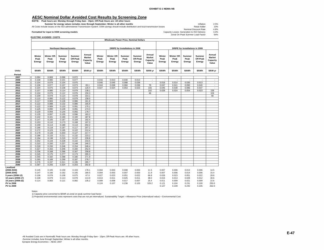
EXHIBIT E-1 NEMA-N$
AESC Nominal Dollar Avoided Cost Results by Screening ZoneNOTE: Peak hours are: Monday through Friday 6am - 10pm; Off-Peak Hours are: All other hours Summer for energy values includes June through September; Winter is all other months Inflation 2.5%All Costs include losses on the ISO-administered Transmission System. DSM savings should include distribution and local transmission losses Retail Adder 10%
Nominal Discount Rate 4.8%Formatted for input to DSM screening models Capacity Losses: Generation to ISO Delivery 3.4%
Zonal On-Peak Summer Load Factor 64%ELECTRIC AVOIDED COSTS
Winter Peak
Energy
Winter Off-Peak
Energy
Summer Peak
Energy
Summer Off-Peak Energy
Annual Market
Capacity Value
Winter Peak
Energy
Winter Off-Peak
Energy
Summer Peak
Energy
Summer Off-Peak Energy
Annual Market
Capacity Value
Winter Peak
Energy
Winter Off-Peak
Energy
Summer Peak
Energy
Summer Off-Peak Energy
Annual Market
Capacity Value
Units: $/kWh $/kWh $/kWh $/kWh $/kW-yr $/kWh $/kWh $/kWh $/kWh $/kW-yr $/kWh $/kWh $/kWh $/kWh $/kW-yr
Period:2007 0.094 0.069 0.096 0.0722008 0.108 0.080 0.101 0.077 0.016 0.013 0.030 0.013 - - - - - - 2009 0.104 0.079 0.104 0.075 0.046 0.040 0.088 0.039 - 0.016 0.014 0.030 0.013 - 2010 0.106 0.077 0.107 0.073 65.1 0.044 0.038 0.084 0.036 78 0.047 0.041 0.090 0.040 - 2011 0.104 0.075 0.108 0.073 120.4 0.027 0.024 0.053 0.023 155 0.045 0.039 0.086 0.037 - 2012 0.107 0.080 0.114 0.079 138.1 102 0.028 0.024 0.054 0.023 1582013 0.104 0.076 0.112 0.076 150.3 46 1042014 0.109 0.078 0.114 0.078 154.1 482015 0.110 0.080 0.122 0.079 158.02016 0.117 0.083 0.126 0.086 161.92017 0.122 0.088 0.132 0.086 165.92018 0.122 0.089 0.133 0.091 170.12019 0.125 0.090 0.139 0.091 174.32020 0.130 0.094 0.144 0.092 178.72021 0.135 0.097 0.155 0.096 183.22022 0.142 0.101 0.160 0.100 187.82023 0.147 0.105 0.167 0.104 192.42024 0.153 0.110 0.173 0.108 197.32025 0.159 0.114 0.180 0.113 202.22026 0.166 0.118 0.187 0.117 207.22027 0.172 0.123 0.195 0.122 212.42028 0.179 0.128 0.203 0.127 217.72029 0.186 0.133 0.211 0.132 223.22030 0.194 0.138 0.219 0.137 228.82031 0.202 0.144 0.228 0.142 234.52032 0.210 0.150 0.237 0.148 240.32033 0.218 0.156 0.246 0.154 246.42034 0.227 0.162 0.256 0.160 252.52035 0.236 0.168 0.266 0.167 258.82036 0.245 0.175 0.277 0.173 265.32037 0.255 0.182 0.288 0.180 271.92038 0.265 0.189 0.299 0.187 278.72039 0.276 0.197 0.311 0.195 285.72040 0.287 0.205 0.324 0.203 292.8
Levelized(2008-2040) 0.145 0.105 0.159 0.103 178.1 0.004 0.003 0.008 0.003 11.5 0.007 0.006 0.013 0.006 14.5(2009-2040) 0.147 0.106 0.162 0.105 180.5 0.004 0.003 0.007 0.003 11.9 0.007 0.006 0.014 0.006 15.45 years (2008-12) 0.106 0.078 0.106 0.075 67.0 0.027 0.023 0.051 0.022 66.8 0.026 0.023 0.051 0.022 28.810 years (2008-17) 0.108 0.079 0.113 0.078 113.9 0.013 0.011 0.025 0.011 38.0 0.015 0.013 0.028 0.012 30.615 years (2008-22) 0.114 0.083 0.121 0.082 135.2 0.009 0.008 0.017 0.007 25.4 0.011 0.009 0.021 0.009 22.6PV to 2008 0.124 0.107 0.236 0.103 326.2 0.121 0.104 0.231 0.100 250.0PV to 2009 0.127 0.109 0.242 0.105 262.0
Notes: 1) Capacity price converted to $/kWh at zonal on-peak summer load factor.2) Projected environmental costs represent costs that are not yet internalized. Sustainability Target = Allowance Price (internalized value) + Environmental Cost
Northeast Massachusetts DRIPE for Installations in 2008 DRIPE for Installations in 2009
Wholesale Power Price, Nominal Dollars
-All Avoided Costs are in Nominal$; Peak hours are: Monday through Friday 6am - 10pm; Off-Peak Hours are: All other hours.-Summer includes June through September; Winter is all other months.Synapse Energy Economics – AESC 2007
E-47

EXHIBIT E-1 NEMA-N$
Units:
Period:2007200820092010201120122013201420152016201720182019202020212022202320242025202620272028202920302031203220332034203520362037203820392040
Levelized(2008-2040)(2009-2040)5 years (2008-12)10 years (2008-17)15 years (2008-22)PV to 2008PV to 2009
AESC Nominal Dollar Avoided Cost Results by Screening ZoneNOTE: Peak hours are: Monday through Friday 6am - 10pm; Off-Peak Hours are: All other hours Summer for energy values includes June through September; Winter is all other monthsAll Costs include losses on the ISO-administered Transmission System. DSM savings should include distribution and local transmission losses
2010-11 60%Formatted for input to DSM screening models 2011-12 80%
2012-13 100%2013-14 100%
REC Costs
Winter Peak
Energy
Winter Off-Peak
Energy
Summer Peak
Energy
Summer Off-Peak Energy
Summer: June, July,
August
Winter: December,
January
On-Peak Summer Capacity
Value1
Winter Peak
Energy
Winter Off-Peak
Energy
Summer Peak
Energy
Summer Off-Peak Energy
Annual Market
Capacity Value
All EnergyWinter Peak
Energy
Winter OffPeak
Energy
Summer Peak
Energy
Summer Off-Peak Energy
Annual Market
Capacity Value
Winter Peak
Energy
Winter OffPeak
Energy
Summer Peak
Energy
Summer Off-Peak Energy
Annual Market
Capacity Value
$/kWh $/kWh $/kWh $/kWh$/kW-month $/kW-month $/kWh $/kWh $/kWh $/kWh $/kWh $/kW-yr ¢/kWh $/kW-yr $/kWh $/kWh $/kWh $/kWh $/kW-yr $/kWh $/kWh $/kWh $/kWh $/kW-yr
0.037 0.036 0.041 0.040 0.084 0.061 0.086 0.064 0.1500.038 0.037 0.042 0.041 9.5 7.2 0.094 0.069 0.088 0.066 0.156 40.5 0.015 0.013 0.029 0.013 - - - - - - 0.037 0.036 0.041 0.040 10.9 8.2 0.088 0.067 0.088 0.063 0.156 45.2 0.044 0.038 0.084 0.037 - 0.015 0.013 0.029 0.013 - 0.038 0.037 0.042 0.041 21.2 15.9 0.075 0.088 0.063 0.088 0.060 67 0.167 19.0 0.041 0.035 0.078 0.034 72 0.044 0.038 0.084 0.037 - 0.039 0.038 0.043 0.042 28.9 21.7 0.138 0.084 0.060 0.087 0.059 114 0.181 0.025 0.021 0.048 0.021 140 0.041 0.035 0.078 0.034 - 0.035 0.034 0.039 0.038 29.6 22.2 0.158 0.084 0.062 0.089 0.062 114 0.189 90 0.025 0.021 0.048 0.021 1400.034 0.034 0.038 0.037 30.4 22.8 0.172 0.079 0.057 0.086 0.057 114 0.191 40 900.034 0.033 0.037 0.036 31.1 23.3 0.176 0.081 0.058 0.085 0.058 114 0.187 400.033 0.032 0.037 0.036 31.9 23.9 0.181 0.080 0.058 0.089 0.057 114 0.1760.032 0.032 0.036 0.035 32.7 24.5 0.185 0.083 0.059 0.090 0.061 114 0.1550.031 0.031 0.035 0.034 33.5 25.1 0.190 0.085 0.061 0.092 0.060 114 0.1270.030 0.030 0.034 0.033 34.4 25.8 0.195 0.084 0.061 0.092 0.062 114 0.0920.029 0.029 0.033 0.032 35.2 26.4 0.200 0.084 0.060 0.094 0.061 114 0.0490.028 0.028 0.032 0.031 36.1 27.1 0.205 0.085 0.062 0.095 0.061 114 0.0000.028 0.028 0.031 0.030 37.0 27.8 0.210 0.087 0.063 0.099 0.062 114 0.0000.028 0.027 0.031 0.030 37.9 28.4 0.215 0.089 0.064 0.101 0.063 114 0.0000.029 0.028 0.032 0.031 38.9 29.2 0.220 0.090 0.065 0.102 0.064 1140.029 0.029 0.033 0.032 39.9 29.9 0.226 0.092 0.065 0.103 0.065 1140.030 0.030 0.034 0.033 40.8 30.6 0.232 0.093 0.066 0.105 0.066 1140.031 0.030 0.034 0.033 41.9 31.4 0.237 0.094 0.067 0.107 0.067 1140.032 0.031 0.035 0.034 42.9 32.2 0.243 0.096 0.068 0.108 0.068 1140.032 0.032 0.036 0.035 44.0 33.0 0.249 0.097 0.069 0.110 0.069 1140.033 0.033 0.037 0.036 45.1 33.8 0.256 0.098 0.070 0.111 0.070 1140.034 0.033 0.038 0.037 46.2 34.7 0.262 0.100 0.071 0.113 0.071 1140.035 0.034 0.039 0.038 47.4 35.5 0.268 0.101 0.072 0.114 0.072 1140.036 0.035 0.040 0.039 48.6 36.4 0.275 0.103 0.073 0.116 0.073 1140.037 0.036 0.041 0.040 49.8 37.3 0.282 0.104 0.074 0.118 0.074 1140.038 0.037 0.042 0.041 51.0 38.3 0.289 0.106 0.076 0.120 0.075 1140.039 0.038 0.043 0.042 52.3 39.2 0.296 0.107 0.077 0.121 0.076 1140.039 0.039 0.044 0.043 53.6 40.2 0.304 0.109 0.078 0.123 0.077 1140.040 0.040 0.045 0.044 54.9 41.2 0.311 0.110 0.079 0.125 0.078 1140.041 0.041 0.046 0.045 56.3 42.2 0.319 0.112 0.080 0.127 0.079 1140.043 0.042 0.047 0.046 57.7 43.3 0.327 0.114 0.081 0.128 0.080 1140.044 0.043 0.049 0.047 59.2 44.4 0.335 0.115 0.082 0.130 0.082 114
0.034 0.034 0.038 0.037 39.7 29.8 0.2010.034 0.034 0.038 0.037 40.7 30.5 0.2050.037 0.037 0.041 0.040 20.0 15.0 0.0160.035 0.034 0.039 0.038 26.0 19.5 0.0930.033 0.032 0.037 0.036 29.4 22.0 0.128
Notes: 1) Capacity price converted to $/kWh at zonal on-peak summer load factor.2) Projected environmental costs represent costs that are not yet internalized. Sustainability Target = Allowance Price (internalized value) + Environmental Cost
DRIPE for Installations in 2008 DRIPE for Installations in 2009
Inputs (Real 2007$)
ICAP
Wholesale Power Price, Nominal Dollars
FCM phase-in
Avoided Costs before Adders and inflationAdditional CO2 Costs
(see note below)
FCM Revenue(not an avoided cost;
do not add to avoided costs)
-All Avoided Costs are in Nominal$; Peak hours are: Monday through Friday 6am - 10pm; Off-Peak Hours are: All other hours.-Summer includes June through September; Winter is all other months.Synapse Energy Economics – AESC 2007
E-48

EXHIBIT E-1 SEMA-N$
AESC Nominal Dollar Avoided Cost Results by Screening ZoneNOTE: Peak hours are: Monday through Friday 6am - 10pm; Off-Peak Hours are: All other hours Summer for energy values includes June through September; Winter is all other months Inflation 2.5%All Costs include losses on the ISO-administered Transmission System. DSM savings should include distribution and local transmission losses Retail Adder 10%
Nominal Discount Rate 4.8%Formatted for input to DSM screening models Capacity Losses: Generation to ISO Delivery 3.4%
Zonal On-Peak Summer Load Factor 57%ELECTRIC AVOIDED COSTS
Winter Peak
Energy
Winter Off-Peak
Energy
Summer Peak
Energy
Summer Off-Peak Energy
Annual Market
Capacity Value
Winter Peak
Energy
Winter Off-Peak
Energy
Summer Peak
Energy
Summer Off-Peak Energy
Annual Market
Capacity Value
Winter Peak
Energy
Winter Off-Peak
Energy
Summer Peak
Energy
Summer Off-Peak Energy
Annual Market
Capacity Value
Units: $/kWh $/kWh $/kWh $/kWh $/kW-yr $/kWh $/kWh $/kWh $/kWh $/kW-yr $/kWh $/kWh $/kWh $/kWh $/kW-yr
Period:2007 0.093 0.068 0.094 0.070 - 2008 0.107 0.079 0.098 0.074 - 0.019 0.014 0.032 0.013 - - - - - - 2009 0.102 0.078 0.101 0.071 - 0.055 0.043 0.095 0.039 - 0.019 0.015 0.033 0.013 - 2010 0.103 0.076 0.104 0.071 65.1 0.052 0.041 0.090 0.036 78 0.056 0.044 0.097 0.040 - 2011 0.101 0.074 0.104 0.070 120.4 0.033 0.025 0.056 0.023 155 0.053 0.042 0.092 0.037 - 2012 0.104 0.078 0.109 0.075 138.1 102 0.033 0.026 0.058 0.023 1582013 0.101 0.074 0.106 0.073 150.3 46 1042014 0.107 0.076 0.110 0.076 154.1 482015 0.108 0.078 0.118 0.076 158.02016 0.112 0.082 0.121 0.081 161.92017 0.119 0.086 0.128 0.085 165.92018 0.120 0.087 0.130 0.087 170.12019 0.122 0.088 0.137 0.088 174.32020 0.125 0.093 0.140 0.091 178.72021 0.131 0.095 0.151 0.094 183.22022 0.140 0.099 0.157 0.099 187.82023 0.145 0.103 0.163 0.103 192.42024 0.151 0.107 0.170 0.107 197.32025 0.157 0.111 0.176 0.112 202.22026 0.163 0.116 0.184 0.116 207.22027 0.170 0.120 0.191 0.121 212.42028 0.177 0.125 0.198 0.126 217.72029 0.184 0.130 0.206 0.131 223.22030 0.191 0.135 0.215 0.136 228.82031 0.198 0.141 0.223 0.141 234.52032 0.206 0.146 0.232 0.147 240.32033 0.215 0.152 0.241 0.153 246.42034 0.223 0.158 0.251 0.159 252.52035 0.232 0.165 0.261 0.165 258.82036 0.241 0.171 0.271 0.172 265.32037 0.251 0.178 0.282 0.179 271.92038 0.261 0.185 0.293 0.186 278.72039 0.271 0.192 0.305 0.193 285.72040 0.282 0.200 0.317 0.201 292.8
Levelized(2008-2040) 0.142 0.102 0.155 0.101 162.3 0.009 0.007 0.015 0.006 18.9 0.008 0.007 0.014 0.006 14.5(2009-2040) 0.144 0.104 0.158 0.103 172.3 0.008 0.006 0.014 0.006 20.1 0.009 0.007 0.015 0.006 15.45 years (2008-12) 0.104 0.077 0.103 0.072 61.0 0.032 0.025 0.055 0.022 63.4 0.031 0.025 0.054 0.022 28.810 years (2008-17) 0.106 0.078 0.109 0.075 103.8 0.018 0.014 0.031 0.013 39.9 0.018 0.014 0.030 0.012 30.615 years (2008-22) 0.111 0.082 0.118 0.079 123.1 0.013 0.010 0.023 0.009 29.5 0.013 0.010 0.022 0.009 22.6PV to 2008 0.147 0.115 0.253 0.103 326.2 0.144 0.112 0.247 0.100 250.0PV to 2009 0.150 0.118 0.259 0.105 262.0
Notes: 1) Capacity price converted to $/kWh at zonal on-peak summer load factor.2) Projected environmental costs represent costs that are not yet internalized. Sustainability Target = Allowance Price (internalized value) + Environmental Cost
Southeast Massachusetts DRIPE for Installations in 2008 DRIPE for Installations in 2009
Wholesale Power Price, Nominal Dollars
-All Avoided Costs are in Nominal$; Peak hours are: Monday through Friday 6am - 10pm; Off-Peak Hours are: All other hours.-Summer includes June through September; Winter is all other months.Synapse Energy Economics – AESC 2007
E-49
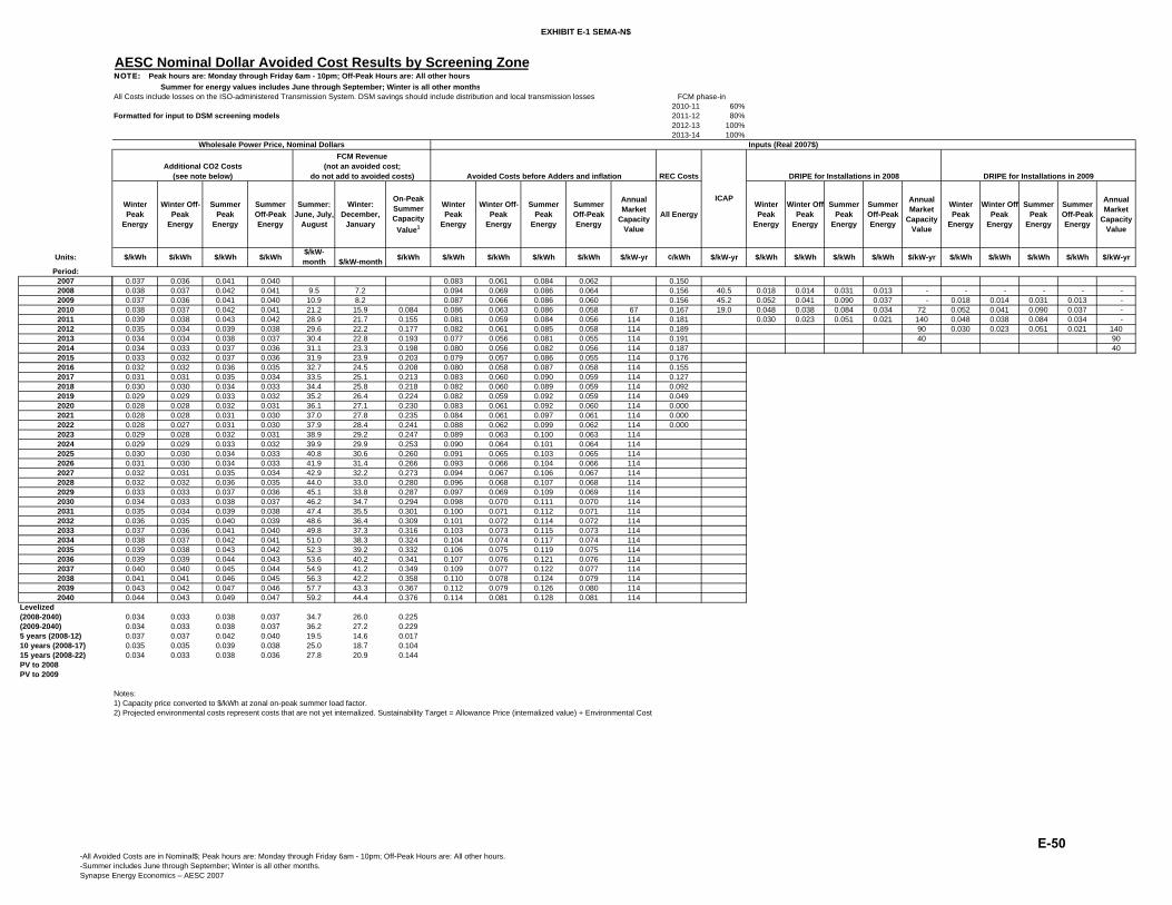
EXHIBIT E-1 SEMA-N$
Units:
Period:2007200820092010201120122013201420152016201720182019202020212022202320242025202620272028202920302031203220332034203520362037203820392040
Levelized(2008-2040)(2009-2040)5 years (2008-12)10 years (2008-17)15 years (2008-22)PV to 2008PV to 2009
AESC Nominal Dollar Avoided Cost Results by Screening ZoneNOTE: Peak hours are: Monday through Friday 6am - 10pm; Off-Peak Hours are: All other hours Summer for energy values includes June through September; Winter is all other monthsAll Costs include losses on the ISO-administered Transmission System. DSM savings should include distribution and local transmission losses
2010-11 60%Formatted for input to DSM screening models 2011-12 80%
2012-13 100%2013-14 100%
REC Costs
Winter Peak
Energy
Winter Off-Peak
Energy
Summer Peak
Energy
Summer Off-Peak Energy
Summer: June, July,
August
Winter: December,
January
On-Peak Summer Capacity
Value1
Winter Peak
Energy
Winter Off-Peak
Energy
Summer Peak
Energy
Summer Off-Peak Energy
Annual Market
Capacity Value
All EnergyWinter Peak
Energy
Winter OffPeak
Energy
Summer Peak
Energy
Summer Off-Peak Energy
Annual Market
Capacity Value
Winter Peak
Energy
Winter OffPeak
Energy
Summer Peak
Energy
Summer Off-Peak Energy
Annual Market
Capacity Value
$/kWh $/kWh $/kWh $/kWh$/kW-month $/kW-month $/kWh $/kWh $/kWh $/kWh $/kWh $/kW-yr ¢/kWh $/kW-yr $/kWh $/kWh $/kWh $/kWh $/kW-yr $/kWh $/kWh $/kWh $/kWh $/kW-yr
0.037 0.036 0.041 0.040 0.083 0.061 0.084 0.062 0.1500.038 0.037 0.042 0.041 9.5 7.2 0.094 0.069 0.086 0.064 0.156 40.5 0.018 0.014 0.031 0.013 - - - - - - 0.037 0.036 0.041 0.040 10.9 8.2 0.087 0.066 0.086 0.060 0.156 45.2 0.052 0.041 0.090 0.037 - 0.018 0.014 0.031 0.013 - 0.038 0.037 0.042 0.041 21.2 15.9 0.084 0.086 0.063 0.086 0.058 67 0.167 19.0 0.048 0.038 0.084 0.034 72 0.052 0.041 0.090 0.037 - 0.039 0.038 0.043 0.042 28.9 21.7 0.155 0.081 0.059 0.084 0.056 114 0.181 0.030 0.023 0.051 0.021 140 0.048 0.038 0.084 0.034 - 0.035 0.034 0.039 0.038 29.6 22.2 0.177 0.082 0.061 0.085 0.058 114 0.189 90 0.030 0.023 0.051 0.021 1400.034 0.034 0.038 0.037 30.4 22.8 0.193 0.077 0.056 0.081 0.055 114 0.191 40 900.034 0.033 0.037 0.036 31.1 23.3 0.198 0.080 0.056 0.082 0.056 114 0.187 400.033 0.032 0.037 0.036 31.9 23.9 0.203 0.079 0.057 0.086 0.055 114 0.1760.032 0.032 0.036 0.035 32.7 24.5 0.208 0.080 0.058 0.087 0.058 114 0.1550.031 0.031 0.035 0.034 33.5 25.1 0.213 0.083 0.060 0.090 0.059 114 0.1270.030 0.030 0.034 0.033 34.4 25.8 0.218 0.082 0.060 0.089 0.059 114 0.0920.029 0.029 0.033 0.032 35.2 26.4 0.224 0.082 0.059 0.092 0.059 114 0.0490.028 0.028 0.032 0.031 36.1 27.1 0.230 0.083 0.061 0.092 0.060 114 0.0000.028 0.028 0.031 0.030 37.0 27.8 0.235 0.084 0.061 0.097 0.061 114 0.0000.028 0.027 0.031 0.030 37.9 28.4 0.241 0.088 0.062 0.099 0.062 114 0.0000.029 0.028 0.032 0.031 38.9 29.2 0.247 0.089 0.063 0.100 0.063 1140.029 0.029 0.033 0.032 39.9 29.9 0.253 0.090 0.064 0.101 0.064 1140.030 0.030 0.034 0.033 40.8 30.6 0.260 0.091 0.065 0.103 0.065 1140.031 0.030 0.034 0.033 41.9 31.4 0.266 0.093 0.066 0.104 0.066 1140.032 0.031 0.035 0.034 42.9 32.2 0.273 0.094 0.067 0.106 0.067 1140.032 0.032 0.036 0.035 44.0 33.0 0.280 0.096 0.068 0.107 0.068 1140.033 0.033 0.037 0.036 45.1 33.8 0.287 0.097 0.069 0.109 0.069 1140.034 0.033 0.038 0.037 46.2 34.7 0.294 0.098 0.070 0.111 0.070 1140.035 0.034 0.039 0.038 47.4 35.5 0.301 0.100 0.071 0.112 0.071 1140.036 0.035 0.040 0.039 48.6 36.4 0.309 0.101 0.072 0.114 0.072 1140.037 0.036 0.041 0.040 49.8 37.3 0.316 0.103 0.073 0.115 0.073 1140.038 0.037 0.042 0.041 51.0 38.3 0.324 0.104 0.074 0.117 0.074 1140.039 0.038 0.043 0.042 52.3 39.2 0.332 0.106 0.075 0.119 0.075 1140.039 0.039 0.044 0.043 53.6 40.2 0.341 0.107 0.076 0.121 0.076 1140.040 0.040 0.045 0.044 54.9 41.2 0.349 0.109 0.077 0.122 0.077 1140.041 0.041 0.046 0.045 56.3 42.2 0.358 0.110 0.078 0.124 0.079 1140.043 0.042 0.047 0.046 57.7 43.3 0.367 0.112 0.079 0.126 0.080 1140.044 0.043 0.049 0.047 59.2 44.4 0.376 0.114 0.081 0.128 0.081 114
0.034 0.033 0.038 0.037 34.7 26.0 0.2250.034 0.033 0.038 0.037 36.2 27.2 0.2290.037 0.037 0.042 0.040 19.5 14.6 0.0170.035 0.035 0.039 0.038 25.0 18.7 0.1040.034 0.033 0.038 0.036 27.8 20.9 0.144
Notes: 1) Capacity price converted to $/kWh at zonal on-peak summer load factor.2) Projected environmental costs represent costs that are not yet internalized. Sustainability Target = Allowance Price (internalized value) + Environmental Cost
DRIPE for Installations in 2008 DRIPE for Installations in 2009
Inputs (Real 2007$)
ICAP
Wholesale Power Price, Nominal Dollars
FCM phase-in
Avoided Costs before Adders and inflationAdditional CO2 Costs
(see note below)
FCM Revenue(not an avoided cost;
do not add to avoided costs)
-All Avoided Costs are in Nominal$; Peak hours are: Monday through Friday 6am - 10pm; Off-Peak Hours are: All other hours.-Summer includes June through September; Winter is all other months.Synapse Energy Economics – AESC 2007
E-50

EXHIBIT E-1 WCMA-N$
AESC Nominal Dollar Avoided Cost Results by Screening ZoneNOTE: Peak hours are: Monday through Friday 6am - 10pm; Off-Peak Hours are: All other hours Summer for energy values includes June through September; Winter is all other months Inflation 2.5%All Costs include losses on the ISO-administered Transmission System. DSM savings should include distribution and local transmission losses Retail Adder 10%
Nominal Discount Rate 4.8%Formatted for input to DSM screening models Capacity Losses: Generation to ISO Delivery 3.4%
Zonal On-Peak Summer Load Factor 60%ELECTRIC AVOIDED COSTS
Winter Peak
Energy
Winter Off-Peak
Energy
Summer Peak
Energy
Summer Off-Peak Energy
Annual Market
Capacity Value
Winter Peak
Energy
Winter Off-Peak
Energy
Summer Peak
Energy
Summer Off-Peak Energy
Annual Market
Capacity Value
Winter Peak
Energy
Winter Off-Peak
Energy
Summer Peak
Energy
Summer Off-Peak Energy
Annual Market
Capacity Value
Units: $/kWh $/kWh $/kWh $/kWh $/kW-yr $/kWh $/kWh $/kWh $/kWh $/kW-yr $/kWh $/kWh $/kWh $/kWh $/kW-yr
Period:2007 0.095 0.070 0.096 0.073 - 2008 0.108 0.082 0.100 0.078 - 0.016 0.012 0.027 0.010 - - - - - - 2009 0.103 0.080 0.102 0.076 - 0.047 0.036 0.080 0.030 - 0.016 0.012 0.027 0.010 - 2010 0.105 0.078 0.105 0.073 65.1 0.045 0.034 0.077 0.029 78 0.048 0.037 0.082 0.031 - 2011 0.103 0.077 0.106 0.073 120.4 0.028 0.021 0.048 0.018 155 0.046 0.035 0.078 0.029 - 2012 0.106 0.080 0.110 0.078 138.1 102 0.029 0.022 0.049 0.018 1582013 0.103 0.076 0.109 0.075 150.3 46 1042014 0.109 0.078 0.112 0.079 154.1 482015 0.109 0.081 0.119 0.081 158.02016 0.115 0.084 0.122 0.086 161.92017 0.120 0.088 0.130 0.088 165.92018 0.120 0.089 0.130 0.090 170.12019 0.122 0.089 0.136 0.089 174.32020 0.129 0.095 0.142 0.094 178.72021 0.132 0.097 0.150 0.097 183.22022 0.139 0.102 0.157 0.101 187.82023 0.145 0.106 0.163 0.105 192.42024 0.151 0.110 0.170 0.109 197.32025 0.157 0.114 0.176 0.114 202.22026 0.163 0.119 0.183 0.118 207.22027 0.170 0.123 0.191 0.123 212.42028 0.176 0.128 0.198 0.128 217.72029 0.183 0.133 0.206 0.133 223.22030 0.191 0.139 0.215 0.138 228.82031 0.198 0.144 0.223 0.144 234.52032 0.206 0.150 0.232 0.149 240.32033 0.214 0.156 0.241 0.155 246.42034 0.223 0.162 0.251 0.161 252.52035 0.232 0.169 0.261 0.168 258.82036 0.241 0.175 0.271 0.175 265.32037 0.251 0.182 0.282 0.181 271.92038 0.261 0.190 0.293 0.189 278.72039 0.271 0.197 0.305 0.196 285.72040 0.282 0.205 0.317 0.204 292.8
Levelized(2008-2040) 0.143 0.105 0.155 0.104 162.3 0.007 0.006 0.012 0.005 18.9 0.007 0.005 0.012 0.005 14.5(2009-2040) 0.145 0.107 0.159 0.105 172.3 0.007 0.005 0.012 0.004 20.1 0.008 0.006 0.013 0.005 15.45 years (2008-12) 0.105 0.080 0.104 0.075 61.0 0.027 0.021 0.047 0.018 63.4 0.027 0.021 0.046 0.017 28.810 years (2008-17) 0.108 0.080 0.110 0.078 103.8 0.015 0.012 0.026 0.010 39.9 0.015 0.011 0.026 0.010 30.615 years (2008-22) 0.113 0.084 0.119 0.082 123.1 0.011 0.009 0.019 0.007 29.5 0.011 0.008 0.019 0.007 22.6PV to 2008 0.125 0.096 0.214 0.080 326.2 0.123 0.094 0.210 0.078 250.0PV to 2009 0.128 0.098 0.220 0.082 262.0
Notes: 1) Capacity price converted to $/kWh at zonal on-peak summer load factor.2) Projected environmental costs represent costs that are not yet internalized. Sustainability Target = Allowance Price (internalized value) + Environmental Cost
West-Central Massachusetts DRIPE for Installations in 2008 DRIPE for Installations in 2009
Wholesale Power Price, Nominal Dollars
-All Avoided Costs are in Nominal$; Peak hours are: Monday through Friday 6am - 10pm; Off-Peak Hours are: All other hours.-Summer includes June through September; Winter is all other months.Synapse Energy Economics – AESC 2007
E-51

EXHIBIT E-1 WCMA-N$
Units:
Period:2007200820092010201120122013201420152016201720182019202020212022202320242025202620272028202920302031203220332034203520362037203820392040
Levelized(2008-2040)(2009-2040)5 years (2008-12)10 years (2008-17)15 years (2008-22)PV to 2008PV to 2009
AESC Nominal Dollar Avoided Cost Results by Screening ZoneNOTE: Peak hours are: Monday through Friday 6am - 10pm; Off-Peak Hours are: All other hours Summer for energy values includes June through September; Winter is all other monthsAll Costs include losses on the ISO-administered Transmission System. DSM savings should include distribution and local transmission losses
2010-11 60%Formatted for input to DSM screening models 2011-12 80%
2012-13 100%2013-14 100%
REC Costs
Winter Peak
Energy
Winter Off-Peak
Energy
Summer Peak
Energy
Summer Off-Peak Energy
Summer: June, July,
August
Winter: December,
January
On-Peak Summer Capacity
Value1
Winter Peak
Energy
Winter Off-Peak
Energy
Summer Peak
Energy
Summer Off-Peak Energy
Annual Market
Capacity Value
All EnergyWinter Peak
Energy
Winter OffPeak
Energy
Summer Peak
Energy
Summer Off-Peak Energy
Annual Market
Capacity Value
Winter Peak
Energy
Winter OffPeak
Energy
Summer Peak
Energy
Summer Off-Peak Energy
Annual Market
Capacity Value
$/kWh $/kWh $/kWh $/kWh$/kW-month $/kW-month $/kWh $/kWh $/kWh $/kWh $/kWh $/kW-yr ¢/kWh $/kW-yr $/kWh $/kWh $/kWh $/kWh $/kW-yr $/kWh $/kWh $/kWh $/kWh $/kW-yr
0.037 0.036 0.041 0.040 0.085 0.062 0.086 0.065 0.1500.038 0.037 0.042 0.041 9.5 7.2 0.095 0.071 0.087 0.067 0.156 40.5 0.015 0.012 0.026 0.010 - - - - - - 0.037 0.036 0.041 0.040 10.9 8.2 0.087 0.068 0.086 0.064 0.156 45.2 0.045 0.034 0.076 0.029 - 0.015 0.012 0.026 0.010 - 0.038 0.037 0.042 0.041 21.2 15.9 0.079 0.087 0.064 0.087 0.060 67 0.167 19.0 0.042 0.032 0.071 0.027 72 0.045 0.034 0.076 0.029 - 0.039 0.038 0.043 0.042 28.9 21.7 0.147 0.083 0.062 0.086 0.058 114 0.181 0.025 0.019 0.043 0.016 140 0.042 0.032 0.071 0.027 - 0.035 0.034 0.039 0.038 29.6 22.2 0.168 0.083 0.063 0.087 0.061 114 0.189 90 0.025 0.019 0.043 0.016 1400.034 0.034 0.038 0.037 30.4 22.8 0.183 0.079 0.058 0.083 0.057 114 0.191 40 900.034 0.033 0.037 0.036 31.1 23.3 0.188 0.082 0.058 0.084 0.059 114 0.187 400.033 0.032 0.037 0.036 31.9 23.9 0.193 0.080 0.058 0.087 0.058 114 0.1760.032 0.032 0.036 0.035 32.7 24.5 0.197 0.082 0.060 0.087 0.061 114 0.1550.031 0.031 0.035 0.034 33.5 25.1 0.202 0.084 0.062 0.091 0.061 114 0.1270.030 0.030 0.034 0.033 34.4 25.8 0.207 0.082 0.061 0.089 0.061 114 0.0920.029 0.029 0.033 0.032 35.2 26.4 0.213 0.082 0.060 0.091 0.060 114 0.0490.028 0.028 0.032 0.031 36.1 27.1 0.218 0.085 0.062 0.093 0.062 114 0.0000.028 0.028 0.031 0.030 37.0 27.8 0.223 0.085 0.062 0.097 0.062 114 0.0000.028 0.027 0.031 0.030 37.9 28.4 0.229 0.088 0.064 0.098 0.063 114 0.0000.029 0.028 0.032 0.031 38.9 29.2 0.235 0.089 0.065 0.100 0.064 1140.029 0.029 0.033 0.032 39.9 29.9 0.241 0.090 0.066 0.101 0.065 1140.030 0.030 0.034 0.033 40.8 30.6 0.247 0.091 0.067 0.103 0.066 1140.031 0.030 0.034 0.033 41.9 31.4 0.253 0.093 0.067 0.104 0.067 1140.032 0.031 0.035 0.034 42.9 32.2 0.259 0.094 0.068 0.106 0.068 1140.032 0.032 0.036 0.035 44.0 33.0 0.266 0.095 0.069 0.107 0.069 1140.033 0.033 0.037 0.036 45.1 33.8 0.272 0.097 0.070 0.109 0.070 1140.034 0.033 0.038 0.037 46.2 34.7 0.279 0.098 0.071 0.111 0.071 1140.035 0.034 0.039 0.038 47.4 35.5 0.286 0.100 0.073 0.112 0.072 1140.036 0.035 0.040 0.039 48.6 36.4 0.293 0.101 0.074 0.114 0.073 1140.037 0.036 0.041 0.040 49.8 37.3 0.300 0.103 0.075 0.115 0.074 1140.038 0.037 0.042 0.041 51.0 38.3 0.308 0.104 0.076 0.117 0.075 1140.039 0.038 0.043 0.042 52.3 39.2 0.316 0.106 0.077 0.119 0.076 1140.039 0.039 0.044 0.043 53.6 40.2 0.324 0.107 0.078 0.120 0.078 1140.040 0.040 0.045 0.044 54.9 41.2 0.332 0.109 0.079 0.122 0.079 1140.041 0.041 0.046 0.045 56.3 42.2 0.340 0.110 0.080 0.124 0.080 1140.043 0.042 0.047 0.046 57.7 43.3 0.348 0.112 0.081 0.126 0.081 1140.044 0.043 0.049 0.047 59.2 44.4 0.357 0.113 0.083 0.128 0.082 114
0.034 0.033 0.038 0.037 34.7 26.0 0.2140.034 0.033 0.038 0.037 36.2 27.2 0.2180.037 0.037 0.042 0.040 19.5 14.6 0.0170.035 0.035 0.039 0.038 25.0 18.7 0.0990.034 0.033 0.038 0.036 27.8 20.9 0.137
Notes: 1) Capacity price converted to $/kWh at zonal on-peak summer load factor.2) Projected environmental costs represent costs that are not yet internalized. Sustainability Target = Allowance Price (internalized value) + Environmental Cost
DRIPE for Installations in 2008 DRIPE for Installations in 2009
Inputs (Real 2007$)
ICAP
Wholesale Power Price, Nominal Dollars
FCM phase-in
Avoided Costs before Adders and inflationAdditional CO2 Costs
(see note below)
FCM Revenue(not an avoided cost;
do not add to avoided costs)
-All Avoided Costs are in Nominal$; Peak hours are: Monday through Friday 6am - 10pm; Off-Peak Hours are: All other hours.-Summer includes June through September; Winter is all other months.Synapse Energy Economics – AESC 2007
E-52
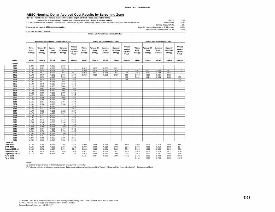
EXHIBIT E-1 non-NEMA-N$
AESC Nominal Dollar Avoided Cost Results by Screening ZoneNOTE: Peak hours are: Monday through Friday 6am - 10pm; Off-Peak Hours are: All other hours Summer for energy values includes June through September; Winter is all other months Inflation 2.5%All Costs include losses on the ISO-administered Transmission System. DSM savings should include distribution and local transmission losses Retail Adder 10%
Nominal Discount Rate 4.8%Formatted for input to DSM screening models Capacity Losses: Generation to ISO Delivery 3.4%
Zonal On-Peak Summer Load Factor 59%ELECTRIC AVOIDED COSTS
Winter Peak
Energy
Winter Off-Peak
Energy
Summer Peak
Energy
Summer Off-Peak Energy
Annual Market
Capacity Value
Winter Peak
Energy
Winter Off-Peak
Energy
Summer Peak
Energy
Summer Off-Peak Energy
Annual Market
Capacity Value
Winter Peak
Energy
Winter Off-Peak
Energy
Summer Peak
Energy
Summer Off-Peak Energy
Annual Market
Capacity Value
Units: $/kWh $/kWh $/kWh $/kWh $/kW-yr $/kWh $/kWh $/kWh $/kWh $/kW-yr $/kWh $/kWh $/kWh $/kWh $/kW-yr
Period:2007 0.094 0.069 0.095 0.072 - 2008 0.108 0.081 0.099 0.076 - 0.017 0.013 0.029 0.011 - - - - - - 2009 0.102 0.079 0.101 0.073 - 0.050 0.039 0.087 0.034 - 0.017 0.013 0.030 0.011 - 2010 0.104 0.077 0.105 0.072 65.1 0.048 0.037 0.083 0.032 78 0.052 0.040 0.089 0.034 - 2011 0.102 0.076 0.105 0.071 120.4 0.030 0.023 0.052 0.020 155 0.049 0.038 0.085 0.033 - 2012 0.105 0.079 0.110 0.076 138.1 102 0.031 0.024 0.053 0.020 1582013 0.102 0.075 0.107 0.074 150.3 46 1042014 0.108 0.077 0.111 0.078 154.1 482015 0.109 0.079 0.118 0.079 158.02016 0.113 0.083 0.122 0.084 161.92017 0.120 0.087 0.129 0.086 165.92018 0.120 0.088 0.130 0.088 170.12019 0.122 0.088 0.136 0.089 174.32020 0.127 0.094 0.141 0.092 178.72021 0.132 0.096 0.151 0.095 183.22022 0.140 0.100 0.157 0.100 187.82023 0.145 0.104 0.163 0.104 192.42024 0.151 0.108 0.170 0.108 197.32025 0.157 0.113 0.176 0.113 202.22026 0.163 0.117 0.183 0.117 207.22027 0.170 0.122 0.191 0.122 212.42028 0.176 0.127 0.198 0.127 217.72029 0.183 0.132 0.206 0.132 223.22030 0.191 0.137 0.215 0.137 228.82031 0.198 0.143 0.223 0.142 234.52032 0.206 0.148 0.232 0.148 240.32033 0.214 0.154 0.241 0.154 246.42034 0.223 0.160 0.251 0.160 252.52035 0.232 0.167 0.261 0.167 258.82036 0.241 0.173 0.271 0.173 265.32037 0.251 0.180 0.282 0.180 271.92038 0.261 0.187 0.293 0.187 278.72039 0.271 0.195 0.305 0.195 285.72040 0.282 0.203 0.317 0.202 292.8
Levelized(2008-2040) 0.142 0.104 0.155 0.102 162.3 0.008 0.006 0.014 0.005 18.9 0.008 0.006 0.013 0.005 14.5(2009-2040) 0.145 0.105 0.159 0.104 172.3 0.007 0.006 0.013 0.005 20.1 0.008 0.006 0.014 0.005 15.45 years (2008-12) 0.104 0.078 0.104 0.074 61.0 0.030 0.023 0.051 0.020 63.4 0.029 0.022 0.050 0.019 28.810 years (2008-17) 0.107 0.079 0.110 0.076 103.8 0.017 0.013 0.028 0.011 39.9 0.016 0.012 0.028 0.011 30.615 years (2008-22) 0.112 0.083 0.118 0.081 123.1 0.012 0.009 0.021 0.008 29.5 0.012 0.009 0.021 0.008 22.6PV to 2008 0.135 0.104 0.233 0.090 326.2 0.132 0.101 0.228 0.088 250.0PV to 2009 0.138 0.106 0.239 0.092 262.0
Notes: 1) Capacity price converted to $/kWh at zonal on-peak summer load factor.2) Projected environmental costs represent costs that are not yet internalized. Sustainability Target = Allowance Price (internalized value) + Environmental Cost
Massachusetts outside of Northeast Mass DRIPE for Installations in 2008 DRIPE for Installations in 2009
Wholesale Power Price, Nominal Dollars
-All Avoided Costs are in Nominal$; Peak hours are: Monday through Friday 6am - 10pm; Off-Peak Hours are: All other hours.-Summer includes June through September; Winter is all other months.Synapse Energy Economics – AESC 2007
E-53
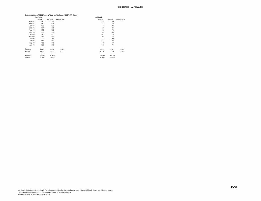
EXHIBIT E-1 non-NEMA-N$
Determination of SEMA and WCMA as % of non-NEMA MA EnergyOn-Peak Off-Peak
SEMA WCMA non-NE MA SEMA WCMA non-NE MAMar-07 560 750 478 704 Feb-07 597 635 533 679 Jan-07 620 823 517 769 Dec-06 574 718 609 815 Nov-06 579 750 532 713 Oct-06 598 579 514 640 Sep-06 585 625 562 785 Aug-06 842 881 609 789 Jul-06 772 769 791 1,005
Jun-06 686 803 524 738 May-06 623 771 469 686 Apr-06 527 670 518 757
Summer 2,885 3,078 5,963 2,485 3,317 5,802 Winter 4,678 5,695 10,373 4,170 5,764 9,935
Summer 48.4% 51.6% 42.8% 57.2%Winter 45.1% 54.9% 42.0% 58.0%
-All Avoided Costs are in Nominal$; Peak hours are: Monday through Friday 6am - 10pm; Off-Peak Hours are: All other hours.-Summer includes June through September; Winter is all other months.Synapse Energy Economics – AESC 2007
E-54
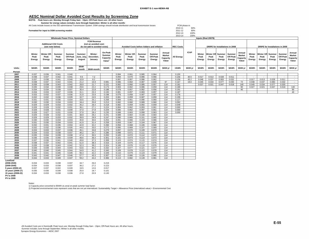
EXHIBIT E-1 non-NEMA-N$
Units:
Period:2007200820092010201120122013201420152016201720182019202020212022202320242025202620272028202920302031203220332034203520362037203820392040
Levelized(2008-2040)(2009-2040)5 years (2008-12)10 years (2008-17)15 years (2008-22)PV to 2008PV to 2009
AESC Nominal Dollar Avoided Cost Results by Screening ZoneNOTE: Peak hours are: Monday through Friday 6am - 10pm; Off-Peak Hours are: All other hours Summer for energy values includes June through September; Winter is all other monthsAll Costs include losses on the ISO-administered Transmission System. DSM savings should include distribution and local transmission losses
2010-11 60%Formatted for input to DSM screening models 2011-12 80%
2012-13 100%2013-14 100%
REC Costs
Winter Peak
Energy
Winter Off-Peak
Energy
Summer Peak
Energy
Summer Off-Peak Energy
Summer: June, July,
August
Winter: December,
January
On-Peak Summer Capacity
Value1
Winter Peak
Energy
Winter Off-Peak
Energy
Summer Peak
Energy
Summer Off-Peak Energy
Annual Market
Capacity Value
All EnergyWinter Peak
Energy
Winter OffPeak
Energy
Summer Peak
Energy
Summer Off-Peak Energy
Annual Market
Capacity Value
Winter Peak
Energy
Winter OffPeak
Energy
Summer Peak
Energy
Summer Off-Peak Energy
Annual Market
Capacity Value
$/kWh $/kWh $/kWh $/kWh$/kW-month $/kW-month $/kWh $/kWh $/kWh $/kWh $/kWh $/kW-yr ¢/kWh $/kW-yr $/kWh $/kWh $/kWh $/kWh $/kW-yr $/kWh $/kWh $/kWh $/kWh $/kW-yr
0.037 0.036 0.041 0.040 0.084 0.061 0.085 0.064 0.1500.038 0.037 0.042 0.041 9.5 7.2 0.094 0.070 0.086 0.066 0.156 40.5 0.017 0.013 0.028 0.011 - - - - - - 0.037 0.036 0.041 0.040 10.9 8.2 0.087 0.067 0.086 0.062 0.156 45.2 0.048 0.037 0.083 0.032 - 0.017 0.013 0.028 0.011 - 0.038 0.037 0.042 0.041 21.2 15.9 0.081 0.086 0.064 0.087 0.059 67 0.167 19.0 0.045 0.034 0.077 0.030 72 0.048 0.037 0.083 0.032 - 0.039 0.038 0.043 0.042 28.9 21.7 0.151 0.082 0.060 0.085 0.057 114 0.181 0.027 0.021 0.047 0.018 140 0.045 0.034 0.077 0.030 - 0.035 0.034 0.039 0.038 29.6 22.2 0.173 0.083 0.062 0.086 0.059 114 0.189 90 0.027 0.021 0.047 0.018 1400.034 0.034 0.038 0.037 30.4 22.8 0.188 0.078 0.057 0.082 0.056 114 0.191 40 900.034 0.033 0.037 0.036 31.1 23.3 0.193 0.081 0.057 0.083 0.057 114 0.187 400.033 0.032 0.037 0.036 31.9 23.9 0.198 0.079 0.058 0.087 0.057 114 0.1760.032 0.032 0.036 0.035 32.7 24.5 0.203 0.081 0.059 0.087 0.059 114 0.1550.031 0.031 0.035 0.034 33.5 25.1 0.208 0.084 0.061 0.090 0.060 114 0.1270.030 0.030 0.034 0.033 34.4 25.8 0.213 0.082 0.060 0.089 0.060 114 0.0920.029 0.029 0.033 0.032 35.2 26.4 0.218 0.082 0.059 0.092 0.059 114 0.0490.028 0.028 0.032 0.031 36.1 27.1 0.224 0.084 0.062 0.093 0.061 114 0.0000.028 0.028 0.031 0.030 37.0 27.8 0.229 0.085 0.062 0.097 0.061 114 0.0000.028 0.027 0.031 0.030 37.9 28.4 0.235 0.088 0.063 0.099 0.063 114 0.0000.029 0.028 0.032 0.031 38.9 29.2 0.241 0.089 0.064 0.100 0.064 1140.029 0.029 0.033 0.032 39.9 29.9 0.247 0.090 0.065 0.101 0.065 1140.030 0.030 0.034 0.033 40.8 30.6 0.253 0.091 0.066 0.103 0.066 1140.031 0.030 0.034 0.033 41.9 31.4 0.259 0.093 0.067 0.104 0.067 1140.032 0.031 0.035 0.034 42.9 32.2 0.266 0.094 0.068 0.106 0.068 1140.032 0.032 0.036 0.035 44.0 33.0 0.272 0.095 0.069 0.107 0.069 1140.033 0.033 0.037 0.036 45.1 33.8 0.279 0.097 0.070 0.109 0.070 1140.034 0.033 0.038 0.037 46.2 34.7 0.286 0.098 0.071 0.111 0.071 1140.035 0.034 0.039 0.038 47.4 35.5 0.293 0.100 0.072 0.112 0.072 1140.036 0.035 0.040 0.039 48.6 36.4 0.301 0.101 0.073 0.114 0.073 1140.037 0.036 0.041 0.040 49.8 37.3 0.308 0.103 0.074 0.115 0.074 1140.038 0.037 0.042 0.041 51.0 38.3 0.316 0.104 0.075 0.117 0.075 1140.039 0.038 0.043 0.042 52.3 39.2 0.324 0.106 0.076 0.119 0.076 1140.039 0.039 0.044 0.043 53.6 40.2 0.332 0.107 0.077 0.121 0.077 1140.040 0.040 0.045 0.044 54.9 41.2 0.340 0.109 0.078 0.122 0.078 1140.041 0.041 0.046 0.045 56.3 42.2 0.349 0.110 0.079 0.124 0.079 1140.043 0.042 0.047 0.046 57.7 43.3 0.357 0.112 0.080 0.126 0.080 1140.044 0.043 0.049 0.047 59.2 44.4 0.366 0.113 0.082 0.128 0.081 114
0.034 0.033 0.038 0.037 34.7 26.0 0.2190.034 0.033 0.038 0.037 36.2 27.2 0.2230.037 0.037 0.042 0.040 19.5 14.6 0.0170.035 0.035 0.039 0.038 25.0 18.7 0.1010.034 0.033 0.038 0.036 27.8 20.9 0.140
Notes: 1) Capacity price converted to $/kWh at zonal on-peak summer load factor.2) Projected environmental costs represent costs that are not yet internalized. Sustainability Target = Allowance Price (internalized value) + Environmental Cost
DRIPE for Installations in 2008 DRIPE for Installations in 2009
Inputs (Real 2007$)
ICAP
Wholesale Power Price, Nominal Dollars
FCM phase-in
Avoided Costs before Adders and inflationAdditional CO2 Costs
(see note below)
FCM Revenue(not an avoided cost;
do not add to avoided costs)
-All Avoided Costs are in Nominal$; Peak hours are: Monday through Friday 6am - 10pm; Off-Peak Hours are: All other hours.-Summer includes June through September; Winter is all other months.Synapse Energy Economics – AESC 2007
E-55

EXHIBIT E-1 SWCT-N$
AESC Nominal Dollar Avoided Cost Results by Screening ZoneNOTE: Peak hours are: Monday through Friday 6am - 10pm; Off-Peak Hours are: All other hours Summer for energy values includes June through September; Winter is all other months Inflation 2.5%All Costs include losses on the ISO-administered Transmission System. DSM savings should include distribution and local transmission losses Retail Adder 10%
Nominal Discount Rate 4.8%Formatted for input to DSM screening models Capacity Losses: Generation to ISO Delivery 3.4%
Zonal On-Peak Summer Load Factor 60%ELECTRIC AVOIDED COSTS
Winter Peak
Energy
Winter Off-Peak
Energy
Summer Peak
Energy
Summer Off-Peak Energy
Annual Market
Capacity Value
Winter Peak
Energy
Winter Off-Peak
Energy
Summer Peak
Energy
Summer Off-Peak Energy
Annual Market
Capacity Value
Winter Peak
Energy
Winter Off-Peak
Energy
Summer Peak
Energy
Summer Off-Peak Energy
Annual Market
Capacity Value
Units: $/kWh $/kWh $/kWh $/kWh $/kW-yr $/kWh $/kWh $/kWh $/kWh $/kW-yr $/kWh $/kWh $/kWh $/kWh $/kW-yr
Period:2007 0.100 0.073 0.105 0.0762008 0.114 0.085 0.110 0.083 0.017 0.014 0.034 0.017 - - - - - - 2009 0.110 0.084 0.113 0.078 0.051 0.041 0.105 0.053 - 0.017 0.014 0.035 0.017 - 2010 0.110 0.082 0.113 0.077 65.1 0.050 0.040 0.105 0.053 78 0.052 0.042 0.108 0.054 - 2011 0.108 0.079 0.115 0.077 120.4 0.031 0.025 0.065 0.033 155 0.051 0.041 0.107 0.055 - 2012 0.111 0.082 0.122 0.080 138.1 102 0.032 0.026 0.067 0.034 1582013 0.109 0.078 0.117 0.077 150.3 46 1042014 0.113 0.079 0.119 0.079 154.1 482015 0.113 0.082 0.122 0.080 158.02016 0.117 0.086 0.128 0.084 161.92017 0.125 0.090 0.137 0.089 165.92018 0.126 0.093 0.137 0.092 170.12019 0.127 0.092 0.142 0.092 174.32020 0.134 0.099 0.150 0.096 178.72021 0.137 0.101 0.157 0.099 183.22022 0.146 0.104 0.166 0.104 187.82023 0.151 0.108 0.172 0.108 192.42024 0.157 0.113 0.179 0.112 197.32025 0.164 0.117 0.186 0.117 202.22026 0.170 0.122 0.194 0.122 207.22027 0.177 0.127 0.201 0.126 212.42028 0.184 0.132 0.209 0.131 217.72029 0.191 0.137 0.218 0.137 223.22030 0.199 0.143 0.227 0.142 228.82031 0.207 0.148 0.236 0.148 234.52032 0.215 0.154 0.245 0.154 240.32033 0.224 0.160 0.255 0.160 246.42034 0.233 0.167 0.265 0.166 252.52035 0.242 0.173 0.275 0.173 258.82036 0.251 0.180 0.286 0.180 265.32037 0.262 0.187 0.298 0.187 271.92038 0.272 0.195 0.310 0.194 278.72039 0.283 0.203 0.322 0.202 285.72040 0.294 0.211 0.335 0.210 292.8
Levelized(2008-2040) 0.149 0.108 0.165 0.107 178.1 0.005 0.004 0.009 0.005 11.5 0.008 0.006 0.016 0.008 14.5(2009-2040) 0.151 0.110 0.168 0.108 180.5 0.004 0.003 0.009 0.004 11.9 0.008 0.007 0.017 0.009 15.45 years (2008-12) 0.111 0.083 0.114 0.079 67.0 0.030 0.024 0.062 0.031 66.8 0.030 0.024 0.061 0.031 28.810 years (2008-17) 0.113 0.083 0.119 0.080 113.9 0.015 0.012 0.031 0.016 38.0 0.017 0.013 0.034 0.017 30.615 years (2008-22) 0.118 0.086 0.127 0.084 135.2 0.010 0.008 0.021 0.010 25.4 0.012 0.010 0.025 0.013 22.6PV to 2008 0.138 0.112 0.286 0.145 326.2 0.135 0.109 0.280 0.142 250.0PV to 2009 0.142 0.114 0.294 0.149 262.0
Notes: 1) Capacity price converted to $/kWh at zonal on-peak summer load factor.2) Projected environmental costs represent costs that are not yet internalized. Sustainability Target = Allowance Price (internalized value) + Environmental Cost
Southwest Connecticut DRIPE for Installations in 2008 DRIPE for Installations in 2009
Wholesale Power Price, Nominal Dollars
-All Avoided Costs are in Nominal$; Peak hours are: Monday through Friday 6am - 10pm; Off-Peak Hours are: All other hours.-Summer includes June through September; Winter is all other months.Synapse Energy Economics – AESC 2007
E-56

EXHIBIT E-1 SWCT-N$
Units:
Period:2007200820092010201120122013201420152016201720182019202020212022202320242025202620272028202920302031203220332034203520362037203820392040
Levelized(2008-2040)(2009-2040)5 years (2008-12)10 years (2008-17)15 years (2008-22)PV to 2008PV to 2009
AESC Nominal Dollar Avoided Cost Results by Screening ZoneNOTE: Peak hours are: Monday through Friday 6am - 10pm; Off-Peak Hours are: All other hours Summer for energy values includes June through September; Winter is all other monthsAll Costs include losses on the ISO-administered Transmission System. DSM savings should include distribution and local transmission losses
2010-11 60%Formatted for input to DSM screening models 2011-12 80%
2012-13 100%2013-14 100%
REC Costs
Winter Peak
Energy
Winter Off-Peak
Energy
Summer Peak
Energy
Summer Off-Peak Energy
Summer: June, July,
August
Winter: December,
January
On-Peak Summer Capacity
Value1
Winter Peak
Energy
Winter Off-Peak
Energy
Summer Peak
Energy
Summer Off-Peak Energy
Annual Market
Capacity Value
All EnergyWinter Peak
Energy
Winter OffPeak
Energy
Summer Peak
Energy
Summer Off-Peak Energy
Annual Market
Capacity Value
Winter Peak
Energy
Winter OffPeak
Energy
Summer Peak
Energy
Summer Off-Peak Energy
Annual Market
Capacity Value
$/kWh $/kWh $/kWh $/kWh$/kW-month $/kW-month $/kWh $/kWh $/kWh $/kWh $/kWh $/kW-yr ¢/kWh $/kW-yr $/kWh $/kWh $/kWh $/kWh $/kW-yr $/kWh $/kWh $/kWh $/kWh $/kW-yr
0.037 0.036 0.041 0.040 0.089 0.065 0.094 0.068 0.1750.038 0.037 0.042 0.041 9.5 7.2 0.099 0.073 0.095 0.071 0.222 40.5 0.017 0.013 0.033 0.016 - - - - - - 0.037 0.036 0.041 0.040 10.9 8.2 0.093 0.070 0.096 0.065 0.233 45.2 0.049 0.039 0.100 0.051 - 0.017 0.013 0.033 0.016 - 0.038 0.037 0.042 0.041 21.2 15.9 0.079 0.090 0.067 0.093 0.063 67 0.233 19.0 0.046 0.037 0.097 0.050 72 0.049 0.039 0.100 0.051 - 0.039 0.038 0.043 0.042 28.9 21.7 0.147 0.087 0.063 0.092 0.061 114 0.211 0.028 0.023 0.059 0.030 140 0.046 0.037 0.097 0.050 - 0.035 0.034 0.039 0.038 29.6 22.2 0.168 0.087 0.064 0.096 0.062 114 0.189 90 0.028 0.023 0.059 0.030 1400.034 0.034 0.038 0.037 30.4 22.8 0.183 0.083 0.059 0.090 0.059 114 0.167 40 900.034 0.033 0.037 0.036 31.1 23.3 0.187 0.085 0.059 0.090 0.059 114 0.145 400.033 0.032 0.037 0.036 31.9 23.9 0.192 0.083 0.060 0.090 0.058 114 0.1230.032 0.032 0.036 0.035 32.7 24.5 0.197 0.085 0.061 0.093 0.060 114 0.0990.031 0.031 0.035 0.034 33.5 25.1 0.202 0.088 0.063 0.097 0.063 114 0.0740.030 0.030 0.034 0.033 34.4 25.8 0.207 0.087 0.064 0.095 0.063 114 0.0490.029 0.029 0.033 0.032 35.2 26.4 0.212 0.086 0.062 0.095 0.062 114 0.0250.028 0.028 0.032 0.031 36.1 27.1 0.217 0.088 0.065 0.099 0.063 114 0.0000.028 0.028 0.031 0.030 37.0 27.8 0.223 0.088 0.065 0.101 0.063 114 0.0000.028 0.027 0.031 0.030 37.9 28.4 0.228 0.091 0.065 0.104 0.065 114 0.0000.029 0.028 0.032 0.031 38.9 29.2 0.234 0.093 0.066 0.106 0.066 1140.029 0.029 0.033 0.032 39.9 29.9 0.240 0.094 0.067 0.107 0.067 1140.030 0.030 0.034 0.033 40.8 30.6 0.246 0.095 0.068 0.109 0.068 1140.031 0.030 0.034 0.033 41.9 31.4 0.252 0.097 0.069 0.110 0.069 1140.032 0.031 0.035 0.034 42.9 32.2 0.258 0.098 0.070 0.112 0.070 1140.032 0.032 0.036 0.035 44.0 33.0 0.265 0.100 0.071 0.113 0.071 1140.033 0.033 0.037 0.036 45.1 33.8 0.271 0.101 0.072 0.115 0.072 1140.034 0.033 0.038 0.037 46.2 34.7 0.278 0.102 0.073 0.117 0.073 1140.035 0.034 0.039 0.038 47.4 35.5 0.285 0.104 0.075 0.118 0.074 1140.036 0.035 0.040 0.039 48.6 36.4 0.292 0.105 0.076 0.120 0.075 1140.037 0.036 0.041 0.040 49.8 37.3 0.300 0.107 0.077 0.122 0.076 1140.038 0.037 0.042 0.041 51.0 38.3 0.307 0.109 0.078 0.124 0.078 1140.039 0.038 0.043 0.042 52.3 39.2 0.315 0.110 0.079 0.125 0.079 1140.039 0.039 0.044 0.043 53.6 40.2 0.323 0.112 0.080 0.127 0.080 1140.040 0.040 0.045 0.044 54.9 41.2 0.331 0.113 0.081 0.129 0.081 1140.041 0.041 0.046 0.045 56.3 42.2 0.339 0.115 0.082 0.131 0.082 1140.043 0.042 0.047 0.046 57.7 43.3 0.348 0.117 0.084 0.133 0.083 1140.044 0.043 0.049 0.047 59.2 44.4 0.356 0.118 0.085 0.135 0.085 114
0.034 0.034 0.038 0.037 39.7 29.8 0.2130.034 0.034 0.038 0.037 40.7 30.5 0.2170.037 0.037 0.041 0.040 20.0 15.0 0.0160.035 0.034 0.039 0.038 26.0 19.5 0.0990.033 0.032 0.037 0.036 29.4 22.0 0.136
Notes: 1) Capacity price converted to $/kWh at zonal on-peak summer load factor.2) Projected environmental costs represent costs that are not yet internalized. Sustainability Target = Allowance Price (internalized value) + Environmental Cost
DRIPE for Installations in 2008 DRIPE for Installations in 2009
Inputs (Real 2007$)
ICAP
Wholesale Power Price, Nominal Dollars
FCM phase-in
Avoided Costs before Adders and inflationAdditional CO2 Costs
(see note below)
FCM Revenue(not an avoided cost;
do not add to avoided costs)
-All Avoided Costs are in Nominal$; Peak hours are: Monday through Friday 6am - 10pm; Off-Peak Hours are: All other hours.-Summer includes June through September; Winter is all other months.Synapse Energy Economics – AESC 2007
E-57
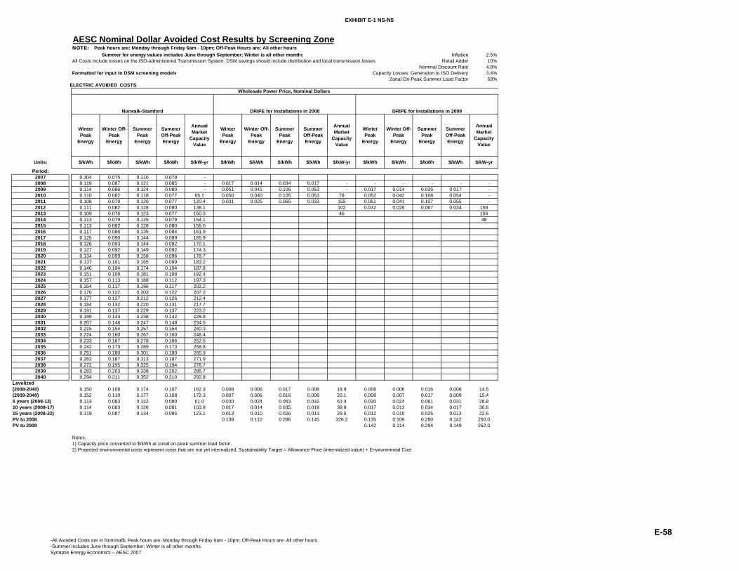
EXHIBIT E-1 NS-N$
AESC Nominal Dollar Avoided Cost Results by Screening ZoneNOTE: Peak hours are: Monday through Friday 6am - 10pm; Off-Peak Hours are: All other hours Summer for energy values includes June through September; Winter is all other months Inflation 2.5%All Costs include losses on the ISO-administered Transmission System. DSM savings should include distribution and local transmission losses Retail Adder 10%
Nominal Discount Rate 4.8%Formatted for input to DSM screening models Capacity Losses: Generation to ISO Delivery 3.4%
Zonal On-Peak Summer Load Factor 59%ELECTRIC AVOIDED COSTS
Winter Peak
Energy
Winter Off-Peak
Energy
Summer Peak
Energy
Summer Off-Peak Energy
Annual Market
Capacity Value
Winter Peak
Energy
Winter Off-Peak
Energy
Summer Peak
Energy
Summer Off-Peak Energy
Annual Market
Capacity Value
Winter Peak
Energy
Winter Off-Peak
Energy
Summer Peak
Energy
Summer Off-Peak Energy
Annual Market
Capacity Value
Units: $/kWh $/kWh $/kWh $/kWh $/kW-yr $/kWh $/kWh $/kWh $/kWh $/kW-yr $/kWh $/kWh $/kWh $/kWh $/kW-yr
Period:2007 0.104 0.075 0.116 0.078 - 2008 0.119 0.087 0.121 0.085 - 0.017 0.014 0.034 0.017 - - - - - - 2009 0.114 0.086 0.124 0.080 - 0.051 0.041 0.105 0.053 - 0.017 0.014 0.035 0.017 - 2010 0.110 0.082 0.118 0.077 65.1 0.050 0.040 0.105 0.053 78 0.052 0.042 0.108 0.054 - 2011 0.108 0.079 0.120 0.077 120.4 0.031 0.025 0.065 0.033 155 0.051 0.041 0.107 0.055 - 2012 0.111 0.082 0.128 0.080 138.1 102 0.032 0.026 0.067 0.034 1582013 0.109 0.078 0.123 0.077 150.3 46 1042014 0.113 0.079 0.125 0.079 154.1 482015 0.113 0.082 0.128 0.080 158.02016 0.117 0.086 0.135 0.084 161.92017 0.125 0.090 0.144 0.089 165.92018 0.126 0.093 0.144 0.092 170.12019 0.127 0.092 0.149 0.092 174.32020 0.134 0.099 0.158 0.096 178.72021 0.137 0.101 0.165 0.099 183.22022 0.146 0.104 0.174 0.104 187.82023 0.151 0.108 0.181 0.108 192.42024 0.157 0.113 0.188 0.112 197.32025 0.164 0.117 0.196 0.117 202.22026 0.170 0.122 0.203 0.122 207.22027 0.177 0.127 0.212 0.126 212.42028 0.184 0.132 0.220 0.131 217.72029 0.191 0.137 0.229 0.137 223.22030 0.199 0.143 0.238 0.142 228.82031 0.207 0.148 0.247 0.148 234.52032 0.215 0.154 0.257 0.154 240.32033 0.224 0.160 0.267 0.160 246.42034 0.233 0.167 0.278 0.166 252.52035 0.242 0.173 0.289 0.173 258.82036 0.251 0.180 0.301 0.180 265.32037 0.262 0.187 0.313 0.187 271.92038 0.272 0.195 0.325 0.194 278.72039 0.283 0.203 0.338 0.202 285.72040 0.294 0.211 0.352 0.210 292.8
Levelized(2008-2040) 0.150 0.108 0.174 0.107 162.3 0.008 0.006 0.017 0.008 18.9 0.008 0.006 0.016 0.008 14.5(2009-2040) 0.152 0.110 0.177 0.108 172.3 0.007 0.006 0.016 0.008 20.1 0.008 0.007 0.017 0.009 15.45 years (2008-12) 0.113 0.083 0.122 0.080 61.0 0.030 0.024 0.063 0.032 63.4 0.030 0.024 0.061 0.031 28.810 years (2008-17) 0.114 0.083 0.126 0.081 103.8 0.017 0.014 0.035 0.018 39.9 0.017 0.013 0.034 0.017 30.615 years (2008-22) 0.119 0.087 0.134 0.085 123.1 0.013 0.010 0.026 0.013 29.5 0.012 0.010 0.025 0.013 22.6PV to 2008 0.138 0.112 0.286 0.145 326.2 0.135 0.109 0.280 0.142 250.0PV to 2009 0.142 0.114 0.294 0.149 262.0
Notes: 1) Capacity price converted to $/kWh at zonal on-peak summer load factor.2) Projected environmental costs represent costs that are not yet internalized. Sustainability Target = Allowance Price (internalized value) + Environmental Cost
Norwalk-Stamford DRIPE for Installations in 2008 DRIPE for Installations in 2009
Wholesale Power Price, Nominal Dollars
-All Avoided Costs are in Nominal$; Peak hours are: Monday through Friday 6am - 10pm; Off-Peak Hours are: All other hours.-Summer includes June through September; Winter is all other months.Synapse Energy Economics – AESC 2007
E-58

EXHIBIT E-1 NS-N$
Units:
Period:2007200820092010201120122013201420152016201720182019202020212022202320242025202620272028202920302031203220332034203520362037203820392040
Levelized(2008-2040)(2009-2040)5 years (2008-12)10 years (2008-17)15 years (2008-22)PV to 2008PV to 2009
AESC Nominal Dollar Avoided Cost Results by Screening ZoneNOTE: Peak hours are: Monday through Friday 6am - 10pm; Off-Peak Hours are: All other hours Summer for energy values includes June through September; Winter is all other monthsAll Costs include losses on the ISO-administered Transmission System. DSM savings should include distribution and local transmission losses
2010-11 60%Formatted for input to DSM screening models 2011-12 80%
2012-13 100%2013-14 100%
REC Costs
Winter Peak
Energy
Winter Off-Peak
Energy
Summer Peak
Energy
Summer Off-Peak Energy
Summer: June, July,
August
Winter: December,
January
On-Peak Summer Capacity
Value1
Winter Peak
Energy
Winter Off-Peak
Energy
Summer Peak
Energy
Summer Off-Peak Energy
Annual Market
Capacity Value
All EnergyWinter Peak
Energy
Winter OffPeak
Energy
Summer Peak
Energy
Summer Off-Peak Energy
Annual Market
Capacity Value
Winter Peak
Energy
Winter OffPeak
Energy
Summer Peak
Energy
Summer Off-Peak Energy
Annual Market
Capacity Value
$/kWh $/kWh $/kWh $/kWh$/kW-month $/kW-month $/kWh $/kWh $/kWh $/kWh $/kWh $/kW-yr ¢/kWh $/kW-yr $/kWh $/kWh $/kWh $/kWh $/kW-yr $/kWh $/kWh $/kWh $/kWh $/kW-yr
0.037 0.036 0.041 0.040 0.093 0.066 0.104 0.069 0.1750.038 0.037 0.042 0.041 9.5 7.2 0.103 0.075 0.105 0.073 0.222 40.5 0.017 0.013 0.033 0.016 - - - - - - 0.037 0.036 0.041 0.040 10.9 8.2 0.096 0.072 0.105 0.067 0.233 45.2 0.049 0.039 0.100 0.051 - 0.017 0.013 0.033 0.016 - 0.038 0.037 0.042 0.041 21.2 15.9 0.081 0.090 0.067 0.097 0.063 67 0.233 19.0 0.046 0.037 0.097 0.050 72 0.049 0.039 0.100 0.051 - 0.039 0.038 0.043 0.042 28.9 21.7 0.149 0.087 0.063 0.097 0.061 114 0.211 0.028 0.023 0.059 0.030 140 0.046 0.037 0.097 0.050 - 0.035 0.034 0.039 0.038 29.6 22.2 0.171 0.087 0.064 0.101 0.062 114 0.189 90 0.028 0.023 0.059 0.030 1400.034 0.034 0.038 0.037 30.4 22.8 0.187 0.083 0.059 0.095 0.059 114 0.167 40 900.034 0.033 0.037 0.036 31.1 23.3 0.191 0.085 0.059 0.094 0.059 114 0.145 400.033 0.032 0.037 0.036 31.9 23.9 0.196 0.083 0.060 0.095 0.058 114 0.1230.032 0.032 0.036 0.035 32.7 24.5 0.201 0.085 0.061 0.097 0.060 114 0.0990.031 0.031 0.035 0.034 33.5 25.1 0.206 0.088 0.063 0.101 0.063 114 0.0740.030 0.030 0.034 0.033 34.4 25.8 0.211 0.087 0.064 0.099 0.063 114 0.0490.029 0.029 0.033 0.032 35.2 26.4 0.216 0.086 0.062 0.100 0.062 114 0.0250.028 0.028 0.032 0.031 36.1 27.1 0.222 0.088 0.065 0.104 0.063 114 0.0000.028 0.028 0.031 0.030 37.0 27.8 0.227 0.088 0.065 0.106 0.063 114 0.0000.028 0.027 0.031 0.030 37.9 28.4 0.233 0.091 0.065 0.109 0.065 114 0.0000.029 0.028 0.032 0.031 38.9 29.2 0.239 0.093 0.066 0.111 0.066 1140.029 0.029 0.033 0.032 39.9 29.9 0.245 0.094 0.067 0.112 0.067 1140.030 0.030 0.034 0.033 40.8 30.6 0.251 0.095 0.068 0.114 0.068 1140.031 0.030 0.034 0.033 41.9 31.4 0.257 0.097 0.069 0.116 0.069 1140.032 0.031 0.035 0.034 42.9 32.2 0.264 0.098 0.070 0.117 0.070 1140.032 0.032 0.036 0.035 44.0 33.0 0.270 0.100 0.071 0.119 0.071 1140.033 0.033 0.037 0.036 45.1 33.8 0.277 0.101 0.072 0.121 0.072 1140.034 0.033 0.038 0.037 46.2 34.7 0.284 0.102 0.073 0.123 0.073 1140.035 0.034 0.039 0.038 47.4 35.5 0.291 0.104 0.075 0.124 0.074 1140.036 0.035 0.040 0.039 48.6 36.4 0.298 0.105 0.076 0.126 0.075 1140.037 0.036 0.041 0.040 49.8 37.3 0.306 0.107 0.077 0.128 0.076 1140.038 0.037 0.042 0.041 51.0 38.3 0.313 0.109 0.078 0.130 0.078 1140.039 0.038 0.043 0.042 52.3 39.2 0.321 0.110 0.079 0.132 0.079 1140.039 0.039 0.044 0.043 53.6 40.2 0.329 0.112 0.080 0.134 0.080 1140.040 0.040 0.045 0.044 54.9 41.2 0.338 0.113 0.081 0.136 0.081 1140.041 0.041 0.046 0.045 56.3 42.2 0.346 0.115 0.082 0.137 0.082 1140.043 0.042 0.047 0.046 57.7 43.3 0.355 0.117 0.084 0.139 0.083 1140.044 0.043 0.049 0.047 59.2 44.4 0.363 0.118 0.085 0.142 0.085 114
0.034 0.033 0.038 0.037 34.7 26.0 0.2180.034 0.033 0.038 0.037 36.2 27.2 0.2220.037 0.037 0.042 0.040 19.5 14.6 0.0170.035 0.035 0.039 0.038 25.0 18.7 0.1010.034 0.033 0.038 0.036 27.8 20.9 0.139
Notes: 1) Capacity price converted to $/kWh at zonal on-peak summer load factor.2) Projected environmental costs represent costs that are not yet internalized. Sustainability Target = Allowance Price (internalized value) + Environmental Cost
DRIPE for Installations in 2008 DRIPE for Installations in 2009
Inputs (Real 2007$)
ICAP
Wholesale Power Price, Nominal Dollars
FCM phase-in
Avoided Costs before Adders and inflationAdditional CO2 Costs
(see note below)
FCM Revenue(not an avoided cost;
do not add to avoided costs)
-All Avoided Costs are in Nominal$; Peak hours are: Monday through Friday 6am - 10pm; Off-Peak Hours are: All other hours.-Summer includes June through September; Winter is all other months.Synapse Energy Economics – AESC 2007
E-59

EXHIBIT E-1 SW-NS-N$
AESC Nominal Dollar Avoided Cost Results by Screening ZoneNOTE: Peak hours are: Monday through Friday 6am - 10pm; Off-Peak Hours are: All other hours Summer for energy values includes June through September; Winter is all other months Inflation 2.5%All Costs include losses on the ISO-administered Transmission System. DSM savings should include distribution and local transmission losses Retail Adder 10%
Nominal Discount Rate 4.8%Formatted for input to DSM screening models Capacity Losses: Generation to ISO Delivery 3.4%
Zonal On-Peak Summer Load Factor 61%ELECTRIC AVOIDED COSTS
Winter Peak
Energy
Winter Off-Peak
Energy
Summer Peak
Energy
Summer Off-Peak Energy
Annual Market
Capacity Value
Winter Peak
Energy
Winter Off-Peak
Energy
Summer Peak
Energy
Summer Off-Peak Energy
Annual Market
Capacity Value
Winter Peak
Energy
Winter Off-Peak
Energy
Summer Peak
Energy
Summer Off-Peak Energy
Annual Market
Capacity Value
Units: $/kWh $/kWh $/kWh $/kWh $/kW-yr $/kWh $/kWh $/kWh $/kWh $/kW-yr $/kWh $/kWh $/kWh $/kWh $/kW-yr
Period:2007 0.098 0.073 0.100 0.076 - 2008 0.112 0.084 0.104 0.082 - 0.017 0.014 0.034 0.017 - - - - - - 2009 0.108 0.083 0.107 0.077 - 0.051 0.041 0.105 0.053 - 0.017 0.014 0.035 0.017 - 2010 0.110 0.082 0.110 0.077 65.1 0.050 0.040 0.105 0.053 78 0.052 0.042 0.108 0.054 - 2011 0.108 0.079 0.112 0.077 120.4 0.031 0.025 0.065 0.033 155 0.051 0.041 0.107 0.055 - 2012 0.111 0.082 0.119 0.080 138.1 102 0.032 0.026 0.067 0.034 1582013 0.109 0.078 0.114 0.077 150.3 46 1042014 0.113 0.079 0.116 0.079 154.1 482015 0.113 0.082 0.119 0.080 158.02016 0.117 0.086 0.125 0.084 161.92017 0.125 0.090 0.133 0.089 165.92018 0.126 0.093 0.134 0.092 170.12019 0.127 0.092 0.138 0.092 174.32020 0.134 0.099 0.146 0.096 178.72021 0.137 0.101 0.153 0.099 183.22022 0.146 0.104 0.161 0.104 187.82023 0.151 0.108 0.168 0.108 192.42024 0.157 0.113 0.174 0.112 197.32025 0.164 0.117 0.181 0.117 202.22026 0.170 0.122 0.189 0.122 207.22027 0.177 0.127 0.196 0.126 212.42028 0.184 0.132 0.204 0.131 217.72029 0.191 0.137 0.212 0.137 223.22030 0.199 0.143 0.220 0.142 228.82031 0.207 0.148 0.229 0.148 234.52032 0.215 0.154 0.238 0.154 240.32033 0.224 0.160 0.248 0.160 246.42034 0.233 0.167 0.258 0.166 252.52035 0.242 0.173 0.268 0.173 258.82036 0.251 0.180 0.279 0.180 265.32037 0.262 0.187 0.290 0.187 271.92038 0.272 0.195 0.301 0.194 278.72039 0.283 0.203 0.313 0.202 285.72040 0.294 0.211 0.326 0.210 292.8
Levelized(2008-2040) 0.149 0.108 0.160 0.107 162.3 0.008 0.006 0.017 0.008 18.9 0.008 0.006 0.016 0.008 14.5(2009-2040) 0.151 0.110 0.164 0.108 172.3 0.007 0.006 0.016 0.008 20.1 0.008 0.007 0.017 0.009 15.45 years (2008-12) 0.110 0.082 0.110 0.079 61.0 0.030 0.024 0.063 0.032 63.4 0.030 0.024 0.061 0.031 28.810 years (2008-17) 0.112 0.082 0.115 0.080 103.8 0.017 0.014 0.035 0.018 39.9 0.017 0.013 0.034 0.017 30.615 years (2008-22) 0.118 0.086 0.123 0.084 123.1 0.013 0.010 0.026 0.013 29.5 0.012 0.010 0.025 0.013 22.6PV to 2008 0.138 0.112 0.286 0.145 326.2 0.135 0.109 0.280 0.142 250.0PV to 2009 0.142 0.114 0.294 0.149 262.0
Notes: 1) Capacity price converted to $/kWh at zonal on-peak summer load factor.2) Projected environmental costs represent costs that are not yet internalized. Sustainability Target = Allowance Price (internalized value) + Environmental Cost
Southwest Connecticut except Norwalk-Stamford DRIPE for Installations in 2008 DRIPE for Installations in 2009
Wholesale Power Price, Nominal Dollars
-All Avoided Costs are in Nominal$; Peak hours are: Monday through Friday 6am - 10pm; Off-Peak Hours are: All other hours.-Summer includes June through September; Winter is all other months.Synapse Energy Economics – AESC 2007
E-60

EXHIBIT E-1 SW-NS-N$
Units:
Period:2007200820092010201120122013201420152016201720182019202020212022202320242025202620272028202920302031203220332034203520362037203820392040
Levelized(2008-2040)(2009-2040)5 years (2008-12)10 years (2008-17)15 years (2008-22)PV to 2008PV to 2009
AESC Nominal Dollar Avoided Cost Results by Screening ZoneNOTE: Peak hours are: Monday through Friday 6am - 10pm; Off-Peak Hours are: All other hours Summer for energy values includes June through September; Winter is all other monthsAll Costs include losses on the ISO-administered Transmission System. DSM savings should include distribution and local transmission losses
2010-11 60%Formatted for input to DSM screening models 2011-12 80%
2012-13 100%2013-14 100%
REC Costs
Winter Peak
Energy
Winter Off-Peak
Energy
Summer Peak
Energy
Summer Off-Peak Energy
Summer: June, July,
August
Winter: December,
January
On-Peak Summer Capacity
Value1
Winter Peak
Energy
Winter Off-Peak
Energy
Summer Peak
Energy
Summer Off-Peak Energy
Annual Market
Capacity Value
All EnergyWinter Peak
Energy
Winter OffPeak
Energy
Summer Peak
Energy
Summer Off-Peak Energy
Annual Market
Capacity Value
Winter Peak
Energy
Winter OffPeak
Energy
Summer Peak
Energy
Summer Off-Peak Energy
Annual Market
Capacity Value
$/kWh $/kWh $/kWh $/kWh$/kW-month $/kW-month $/kWh $/kWh $/kWh $/kWh $/kWh $/kW-yr ¢/kWh $/kW-yr $/kWh $/kWh $/kWh $/kWh $/kW-yr $/kWh $/kWh $/kWh $/kWh $/kW-yr
0.037 0.036 0.041 0.040 0.088 0.064 0.089 0.067 0.1750.038 0.037 0.042 0.041 9.5 7.2 0.097 0.073 0.090 0.071 0.222 40.5 0.017 0.013 0.033 0.016 - - - - - - 0.037 0.036 0.041 0.040 10.9 8.2 0.091 0.070 0.090 0.065 0.233 45.2 0.049 0.039 0.100 0.051 - 0.017 0.013 0.033 0.016 - 0.038 0.037 0.042 0.041 21.2 15.9 0.078 0.090 0.067 0.090 0.063 67 0.233 19.0 0.046 0.037 0.097 0.050 72 0.049 0.039 0.100 0.051 - 0.039 0.038 0.043 0.042 28.9 21.7 0.145 0.087 0.063 0.090 0.061 114 0.211 0.028 0.023 0.059 0.030 140 0.046 0.037 0.097 0.050 - 0.035 0.034 0.039 0.038 29.6 22.2 0.166 0.087 0.064 0.093 0.062 114 0.189 90 0.028 0.023 0.059 0.030 1400.034 0.034 0.038 0.037 30.4 22.8 0.181 0.083 0.059 0.088 0.059 114 0.167 40 900.034 0.033 0.037 0.036 31.1 23.3 0.186 0.085 0.059 0.087 0.059 114 0.145 400.033 0.032 0.037 0.036 31.9 23.9 0.190 0.083 0.060 0.088 0.058 114 0.1230.032 0.032 0.036 0.035 32.7 24.5 0.195 0.085 0.061 0.090 0.060 114 0.0990.031 0.031 0.035 0.034 33.5 25.1 0.200 0.088 0.063 0.094 0.063 114 0.0740.030 0.030 0.034 0.033 34.4 25.8 0.205 0.087 0.064 0.092 0.063 114 0.0490.029 0.029 0.033 0.032 35.2 26.4 0.210 0.086 0.062 0.093 0.062 114 0.0250.028 0.028 0.032 0.031 36.1 27.1 0.215 0.088 0.065 0.097 0.063 114 0.0000.028 0.028 0.031 0.030 37.0 27.8 0.221 0.088 0.065 0.098 0.063 114 0.0000.028 0.027 0.031 0.030 37.9 28.4 0.226 0.091 0.065 0.101 0.065 114 0.0000.029 0.028 0.032 0.031 38.9 29.2 0.232 0.093 0.066 0.103 0.066 1140.029 0.029 0.033 0.032 39.9 29.9 0.238 0.094 0.067 0.104 0.067 1140.030 0.030 0.034 0.033 40.8 30.6 0.244 0.095 0.068 0.106 0.068 1140.031 0.030 0.034 0.033 41.9 31.4 0.250 0.097 0.069 0.107 0.069 1140.032 0.031 0.035 0.034 42.9 32.2 0.256 0.098 0.070 0.109 0.070 1140.032 0.032 0.036 0.035 44.0 33.0 0.262 0.100 0.071 0.110 0.071 1140.033 0.033 0.037 0.036 45.1 33.8 0.269 0.101 0.072 0.112 0.072 1140.034 0.033 0.038 0.037 46.2 34.7 0.276 0.102 0.073 0.114 0.073 1140.035 0.034 0.039 0.038 47.4 35.5 0.282 0.104 0.075 0.115 0.074 1140.036 0.035 0.040 0.039 48.6 36.4 0.289 0.105 0.076 0.117 0.075 1140.037 0.036 0.041 0.040 49.8 37.3 0.297 0.107 0.077 0.119 0.076 1140.038 0.037 0.042 0.041 51.0 38.3 0.304 0.109 0.078 0.120 0.078 1140.039 0.038 0.043 0.042 52.3 39.2 0.312 0.110 0.079 0.122 0.079 1140.039 0.039 0.044 0.043 53.6 40.2 0.320 0.112 0.080 0.124 0.080 1140.040 0.040 0.045 0.044 54.9 41.2 0.327 0.113 0.081 0.126 0.081 1140.041 0.041 0.046 0.045 56.3 42.2 0.336 0.115 0.082 0.127 0.082 1140.043 0.042 0.047 0.046 57.7 43.3 0.344 0.117 0.084 0.129 0.083 1140.044 0.043 0.049 0.047 59.2 44.4 0.353 0.118 0.085 0.131 0.085 114
0.034 0.033 0.038 0.037 34.7 26.0 0.2110.034 0.033 0.038 0.037 36.2 27.2 0.2150.037 0.037 0.042 0.040 19.5 14.6 0.0160.035 0.035 0.039 0.038 25.0 18.7 0.0980.034 0.033 0.038 0.036 27.8 20.9 0.135
Notes: 1) Capacity price converted to $/kWh at zonal on-peak summer load factor.2) Projected environmental costs represent costs that are not yet internalized. Sustainability Target = Allowance Price (internalized value) + Environmental Cost
DRIPE for Installations in 2008 DRIPE for Installations in 2009
Inputs (Real 2007$)
ICAP
Wholesale Power Price, Nominal Dollars
FCM phase-in
Avoided Costs before Adders and inflationAdditional CO2 Costs
(see note below)
FCM Revenue(not an avoided cost;
do not add to avoided costs)
-All Avoided Costs are in Nominal$; Peak hours are: Monday through Friday 6am - 10pm; Off-Peak Hours are: All other hours.-Summer includes June through September; Winter is all other months.Synapse Energy Economics – AESC 2007
E-61

EXHIBIT E-1 non-SWCT-N$
AESC Nominal Dollar Avoided Cost Results by Screening ZoneNOTE: Peak hours are: Monday through Friday 6am - 10pm; Off-Peak Hours are: All other hours Summer for energy values includes June through September; Winter is all other months Inflation 2.5%All Costs include losses on the ISO-administered Transmission System. DSM savings should include distribution and local transmission losses Retail Adder 10%
Nominal Discount Rate 4.8%Formatted for input to DSM screening models Capacity Losses: Generation to ISO Delivery 3.4%
Zonal On-Peak Summer Load Factor 60%ELECTRIC AVOIDED COSTS
Winter Peak
Energy
Winter Off-Peak
Energy
Summer Peak
Energy
Summer Off-Peak Energy
Annual Market
Capacity Value
Winter Peak
Energy
Winter Off-Peak
Energy
Summer Peak
Energy
Summer Off-Peak Energy
Annual Market
Capacity Value
Winter Peak
Energy
Winter Off-Peak
Energy
Summer Peak
Energy
Summer Off-Peak Energy
Annual Market
Capacity Value
Units: $/kWh $/kWh $/kWh $/kWh $/kW-yr $/kWh $/kWh $/kWh $/kWh $/kW-yr $/kWh $/kWh $/kWh $/kWh $/kW-yr
Period:2007 0.099 0.072 0.104 0.075 - 2008 0.113 0.084 0.108 0.082 - 0.017 0.014 0.034 0.017 - - - - - - 2009 0.108 0.083 0.111 0.076 - 0.051 0.041 0.105 0.053 - 0.017 0.014 0.035 0.017 - 2010 0.108 0.080 0.111 0.076 65.1 0.050 0.040 0.105 0.053 78 0.052 0.042 0.108 0.054 - 2011 0.106 0.078 0.112 0.075 120.4 0.031 0.025 0.065 0.033 155 0.051 0.041 0.107 0.055 - 2012 0.110 0.081 0.119 0.078 138.1 102 0.032 0.026 0.067 0.034 1582013 0.107 0.076 0.116 0.075 150.3 46 1042014 0.111 0.078 0.117 0.078 154.1 482015 0.111 0.080 0.121 0.079 158.02016 0.115 0.084 0.126 0.083 161.92017 0.123 0.089 0.134 0.088 165.92018 0.124 0.091 0.135 0.090 170.12019 0.125 0.091 0.140 0.090 174.32020 0.131 0.097 0.148 0.094 178.72021 0.135 0.099 0.153 0.097 183.22022 0.144 0.103 0.162 0.102 187.82023 0.149 0.107 0.169 0.106 192.42024 0.155 0.112 0.176 0.111 197.32025 0.161 0.116 0.183 0.115 202.22026 0.168 0.121 0.190 0.120 207.22027 0.174 0.125 0.197 0.124 212.42028 0.181 0.130 0.205 0.129 217.72029 0.189 0.136 0.214 0.134 223.22030 0.196 0.141 0.222 0.140 228.82031 0.204 0.147 0.231 0.145 234.52032 0.212 0.153 0.240 0.151 240.32033 0.221 0.159 0.250 0.157 246.42034 0.229 0.165 0.260 0.163 252.52035 0.239 0.172 0.270 0.170 258.82036 0.248 0.178 0.281 0.177 265.32037 0.258 0.186 0.292 0.184 271.92038 0.268 0.193 0.304 0.191 278.72039 0.279 0.201 0.316 0.199 285.72040 0.290 0.209 0.328 0.207 292.8
Levelized(2008-2040) 0.147 0.107 0.162 0.105 162.3 0.008 0.006 0.017 0.008 18.9 0.008 0.006 0.016 0.008 14.5(2009-2040) 0.149 0.108 0.165 0.106 172.3 0.007 0.006 0.016 0.008 20.1 0.008 0.007 0.017 0.009 15.45 years (2008-12) 0.109 0.081 0.112 0.078 61.0 0.030 0.024 0.063 0.032 63.4 0.030 0.024 0.061 0.031 28.810 years (2008-17) 0.111 0.081 0.117 0.079 103.8 0.017 0.014 0.035 0.018 39.9 0.017 0.013 0.034 0.017 30.615 years (2008-22) 0.116 0.085 0.124 0.083 123.1 0.013 0.010 0.026 0.013 29.5 0.012 0.010 0.025 0.013 22.6PV to 2008 0.138 0.112 0.286 0.145 326.2 0.135 0.109 0.280 0.142 250.0PV to 2009 0.142 0.114 0.294 0.149 262.0
Notes: 1) Capacity price converted to $/kWh at zonal on-peak summer load factor.2) Projected environmental costs represent costs that are not yet internalized. Sustainability Target = Allowance Price (internalized value) + Environmental Cost
Connecticut except Southwest Connecticut DRIPE for Installations in 2008 DRIPE for Installations in 2009
Wholesale Power Price, Nominal Dollars
-All Avoided Costs are in Nominal$; Peak hours are: Monday through Friday 6am - 10pm; Off-Peak Hours are: All other hours.-Summer includes June through September; Winter is all other months.Synapse Energy Economics – AESC 2007
E-62
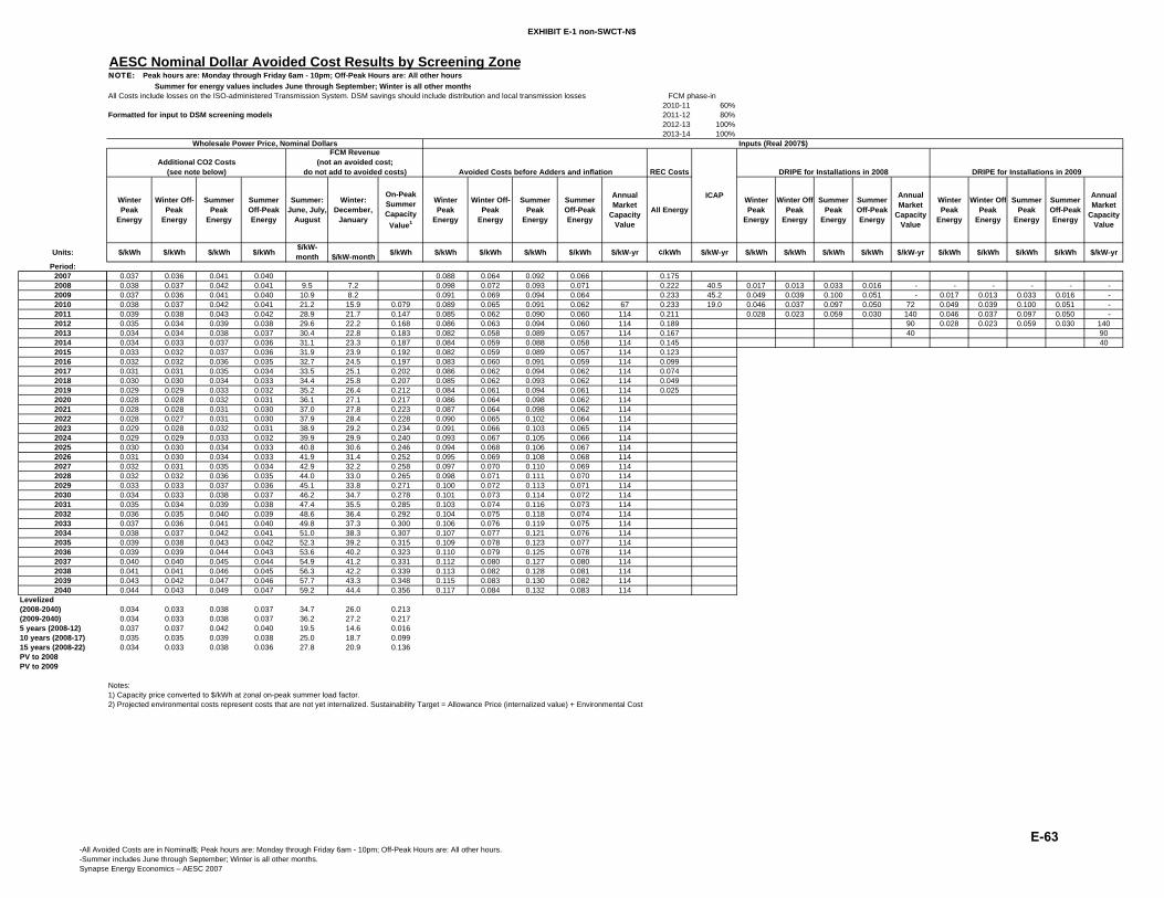
EXHIBIT E-1 non-SWCT-N$
Units:
Period:2007200820092010201120122013201420152016201720182019202020212022202320242025202620272028202920302031203220332034203520362037203820392040
Levelized(2008-2040)(2009-2040)5 years (2008-12)10 years (2008-17)15 years (2008-22)PV to 2008PV to 2009
AESC Nominal Dollar Avoided Cost Results by Screening ZoneNOTE: Peak hours are: Monday through Friday 6am - 10pm; Off-Peak Hours are: All other hours Summer for energy values includes June through September; Winter is all other monthsAll Costs include losses on the ISO-administered Transmission System. DSM savings should include distribution and local transmission losses
2010-11 60%Formatted for input to DSM screening models 2011-12 80%
2012-13 100%2013-14 100%
REC Costs
Winter Peak
Energy
Winter Off-Peak
Energy
Summer Peak
Energy
Summer Off-Peak Energy
Summer: June, July,
August
Winter: December,
January
On-Peak Summer Capacity
Value1
Winter Peak
Energy
Winter Off-Peak
Energy
Summer Peak
Energy
Summer Off-Peak Energy
Annual Market
Capacity Value
All EnergyWinter Peak
Energy
Winter OffPeak
Energy
Summer Peak
Energy
Summer Off-Peak Energy
Annual Market
Capacity Value
Winter Peak
Energy
Winter OffPeak
Energy
Summer Peak
Energy
Summer Off-Peak Energy
Annual Market
Capacity Value
$/kWh $/kWh $/kWh $/kWh$/kW-month $/kW-month $/kWh $/kWh $/kWh $/kWh $/kWh $/kW-yr ¢/kWh $/kW-yr $/kWh $/kWh $/kWh $/kWh $/kW-yr $/kWh $/kWh $/kWh $/kWh $/kW-yr
0.037 0.036 0.041 0.040 0.088 0.064 0.092 0.066 0.1750.038 0.037 0.042 0.041 9.5 7.2 0.098 0.072 0.093 0.071 0.222 40.5 0.017 0.013 0.033 0.016 - - - - - - 0.037 0.036 0.041 0.040 10.9 8.2 0.091 0.069 0.094 0.064 0.233 45.2 0.049 0.039 0.100 0.051 - 0.017 0.013 0.033 0.016 - 0.038 0.037 0.042 0.041 21.2 15.9 0.079 0.089 0.065 0.091 0.062 67 0.233 19.0 0.046 0.037 0.097 0.050 72 0.049 0.039 0.100 0.051 - 0.039 0.038 0.043 0.042 28.9 21.7 0.147 0.085 0.062 0.090 0.060 114 0.211 0.028 0.023 0.059 0.030 140 0.046 0.037 0.097 0.050 - 0.035 0.034 0.039 0.038 29.6 22.2 0.168 0.086 0.063 0.094 0.060 114 0.189 90 0.028 0.023 0.059 0.030 1400.034 0.034 0.038 0.037 30.4 22.8 0.183 0.082 0.058 0.089 0.057 114 0.167 40 900.034 0.033 0.037 0.036 31.1 23.3 0.187 0.084 0.059 0.088 0.058 114 0.145 400.033 0.032 0.037 0.036 31.9 23.9 0.192 0.082 0.059 0.089 0.057 114 0.1230.032 0.032 0.036 0.035 32.7 24.5 0.197 0.083 0.060 0.091 0.059 114 0.0990.031 0.031 0.035 0.034 33.5 25.1 0.202 0.086 0.062 0.094 0.062 114 0.0740.030 0.030 0.034 0.033 34.4 25.8 0.207 0.085 0.062 0.093 0.062 114 0.0490.029 0.029 0.033 0.032 35.2 26.4 0.212 0.084 0.061 0.094 0.061 114 0.0250.028 0.028 0.032 0.031 36.1 27.1 0.217 0.086 0.064 0.098 0.062 1140.028 0.028 0.031 0.030 37.0 27.8 0.223 0.087 0.064 0.098 0.062 1140.028 0.027 0.031 0.030 37.9 28.4 0.228 0.090 0.065 0.102 0.064 1140.029 0.028 0.032 0.031 38.9 29.2 0.234 0.091 0.066 0.103 0.065 1140.029 0.029 0.033 0.032 39.9 29.9 0.240 0.093 0.067 0.105 0.066 1140.030 0.030 0.034 0.033 40.8 30.6 0.246 0.094 0.068 0.106 0.067 1140.031 0.030 0.034 0.033 41.9 31.4 0.252 0.095 0.069 0.108 0.068 1140.032 0.031 0.035 0.034 42.9 32.2 0.258 0.097 0.070 0.110 0.069 1140.032 0.032 0.036 0.035 44.0 33.0 0.265 0.098 0.071 0.111 0.070 1140.033 0.033 0.037 0.036 45.1 33.8 0.271 0.100 0.072 0.113 0.071 1140.034 0.033 0.038 0.037 46.2 34.7 0.278 0.101 0.073 0.114 0.072 1140.035 0.034 0.039 0.038 47.4 35.5 0.285 0.103 0.074 0.116 0.073 1140.036 0.035 0.040 0.039 48.6 36.4 0.292 0.104 0.075 0.118 0.074 1140.037 0.036 0.041 0.040 49.8 37.3 0.300 0.106 0.076 0.119 0.075 1140.038 0.037 0.042 0.041 51.0 38.3 0.307 0.107 0.077 0.121 0.076 1140.039 0.038 0.043 0.042 52.3 39.2 0.315 0.109 0.078 0.123 0.077 1140.039 0.039 0.044 0.043 53.6 40.2 0.323 0.110 0.079 0.125 0.078 1140.040 0.040 0.045 0.044 54.9 41.2 0.331 0.112 0.080 0.127 0.080 1140.041 0.041 0.046 0.045 56.3 42.2 0.339 0.113 0.082 0.128 0.081 1140.043 0.042 0.047 0.046 57.7 43.3 0.348 0.115 0.083 0.130 0.082 1140.044 0.043 0.049 0.047 59.2 44.4 0.356 0.117 0.084 0.132 0.083 114
0.034 0.033 0.038 0.037 34.7 26.0 0.2130.034 0.033 0.038 0.037 36.2 27.2 0.2170.037 0.037 0.042 0.040 19.5 14.6 0.0160.035 0.035 0.039 0.038 25.0 18.7 0.0990.034 0.033 0.038 0.036 27.8 20.9 0.136
Notes: 1) Capacity price converted to $/kWh at zonal on-peak summer load factor.2) Projected environmental costs represent costs that are not yet internalized. Sustainability Target = Allowance Price (internalized value) + Environmental Cost
DRIPE for Installations in 2008 DRIPE for Installations in 2009
Inputs (Real 2007$)
ICAP
Wholesale Power Price, Nominal Dollars
FCM phase-in
Avoided Costs before Adders and inflationAdditional CO2 Costs
(see note below)
FCM Revenue(not an avoided cost;
do not add to avoided costs)
-All Avoided Costs are in Nominal$; Peak hours are: Monday through Friday 6am - 10pm; Off-Peak Hours are: All other hours.-Summer includes June through September; Winter is all other months.Synapse Energy Economics – AESC 2007
E-63