Autonomous Hexapod Walker Robot “Szabad(ka)”uni-obuda.hu/journal/Burkus_Odry_13.pdf“Szabad(ka)” Ervin Burkus, Peter Odry ... The robot’s weight is 1.5 kg. ... The robot’s

Acta Polytechnica Hungarica Vol. 5, No. 1, 2008

– 69 –

Autonomous Hexapod Walker Robot “Szabad(ka)”

Ervin Burkus, Peter Odry Polytechnical Engineering College “VTS” Subotica Marka Oreskovica 16, 24000 Subotica, Serbia [email protected], [email protected]

Abstract: “Szabad(ka)” is a hexapod walker constructed at the Polytechnical Engineering College “VTS” Subotica to test and help implementing algorithms, designed by the Hungarian science institute called ”KFKI”, and our college. These algorithms are connected to combined force and position control, and their primary goal is to achieve robust, adaptable walking in rough and unknown environment, and to calculate the prospective and best route. The article describes the problems which appeared during the process of realization. Starting from the imperfections of the designed construction we describe the justification of the implementation of ANFIS in the further development of the robot.

1 Introduction Walking machines are desirable because they can navigate terrain features that are similar in size to the size of the robot, whereas wheeled and tracked vehicles are only suitable for obstacles smaller than half the diameter of the wheel. Furthermore, if given an ability to find locally horizontal footholds in regionally steep terrain, they can climb extreme angles. Applications potentially include reaching territories which are unreachable or dangerous for humans, exploration, mining, military, rescue, and industrial environments, on earth and beyond.

For walking machines, mostly two legged (biped), four legged (quadruped), and six legged (hexapod) constructions are used. The hexapod is the most stable of the named machines. This is why an autonomous hexapod robot was built with 18 DOFs (degree of freedom) [1].

Before having started building with Szabad(ka) robot, a simplier hexapod robot was built. This robot was the starting point and the source of experience for the designing of Szabad(ka). This hexapod was assembled with -from vitroplast sheets and simple screws. For driving two RC servo motors per feet (2 DOF) were used. The dimensions of the final robot are as follows: 300 mm x 180 mm x 120 mm.

E. Burkus et al. Autonomous Hexapod Walker Robot „Szabad(ka)”

– 70 –

The robot’s weight is 1.5 kg. On the body of the robot there was a single microcontroller and was in contact with the base computer through a radio module as used in modeling. With this robot we controlled the movement of the feet, it was not integrated into the controlling cycle in the feet’s movement algorithm.

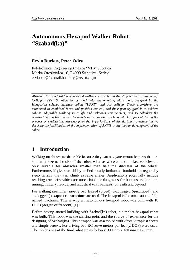
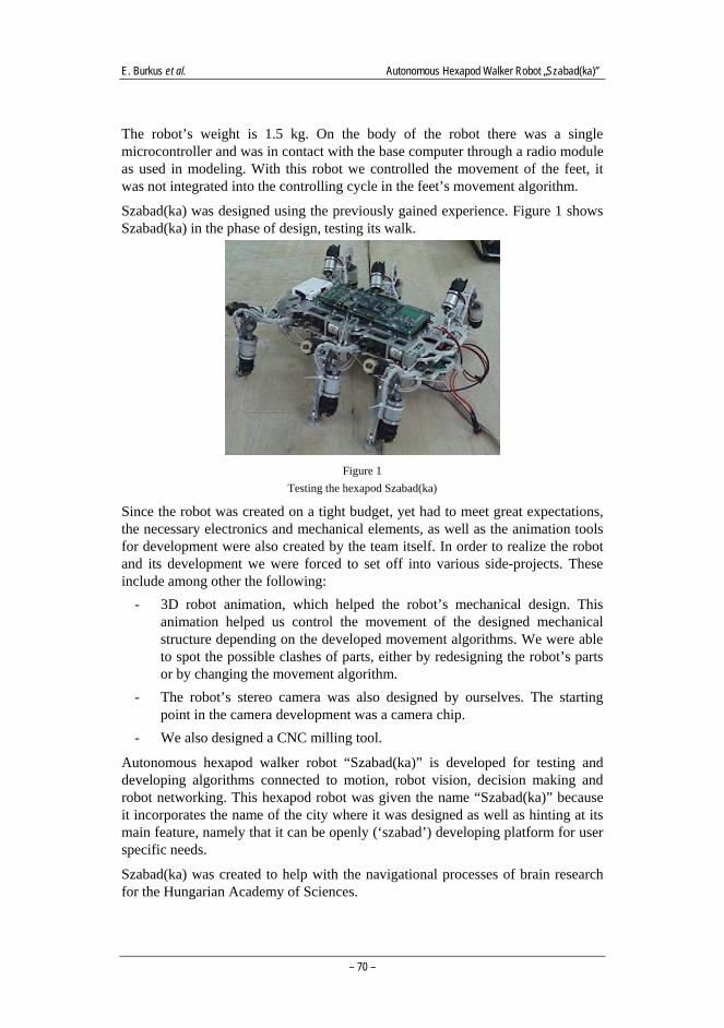
Szabad(ka) was designed using the previously gained experience. Figure 1 shows Szabad(ka) in the phase of design, testing its walk.

Figure 1

Testing the hexapod Szabad(ka)

Since the robot was created on a tight budget, yet had to meet great expectations, the necessary electronics and mechanical elements, as well as the animation tools for development were also created by the team itself. In order to realize the robot and its development we were forced to set off into various side-projects. These include among other the following:

- 3D robot animation, which helped the robot’s mechanical design. This animation helped us control the movement of the designed mechanical structure depending on the developed movement algorithms. We were able to spot the possible clashes of parts, either by redesigning the robot’s parts or by changing the movement algorithm.

- The robot’s stereo camera was also designed by ourselves. The starting point in the camera development was a camera chip.

- We also designed a CNC milling tool.

Autonomous hexapod walker robot “Szabad(ka)” is developed for testing and developing algorithms connected to motion, robot vision, decision making and robot networking. This hexapod robot was given the name “Szabad(ka)” because it incorporates the name of the city where it was designed as well as hinting at its main feature, namely that it can be openly (‘szabad’) developing platform for user specific needs.

Szabad(ka) was created to help with the navigational processes of brain research for the Hungarian Academy of Sciences.


– 71 –

2 Construction of Robot The robot is a complex system both considering its mechanical structure as well as its electronic developments and processor structure.

The robot has MATLAB development platform. It contains one TMS320C6455 DSP (1 GHz frequency) and 10 MSP430F6412 processors, an access point and fully-built it contains 2 cameras, 2 ultra sound radars, several accelerometers, gyroscopes and other sensors for navigation and motion control.

The robot can be used for testing and developing algorithms connected to motion control, visioning, decision making, and networking. In the robot’s 10 microcontrollers, there are various algorithms for sensor processing and basic motion control. Higher level software can be written on personal computers, (in C++ or in MATLAB) and following that it can be implemented into the robots DSP processor which has really high processing abilities. Its software platform (with the already written algorithms) is designed in a modular way, which makes it possible for the developers and researchers to develop codes in their own fields of interest without having to be familiar with other software parts of the robot.

The DSP and the 10 MSP processors are connected into network through SPI and I2C protocols. The DSP processor is on a DSP Starter Kit (DSK) made by a third party company, and the 5 PCB-s (2 MSP controllers on each) are designed at the college. From these 5 boards, 3 are for controlling the legs, and the other two are for processing signals from 2 gyroscopes, 2 accelerometers, 2 radars, several IR collusion detectors. Also every leg has an accelerometer and a force sensor in its foot. The communication with the computer is realized wirelessly with an integrated high speed access point. A Video Interface is implemented for connecting 2 digital, high resolution cameras. This is used for stereo visioning.

The robot’s body is made from more than 150 aluminium and steel parts. All of them were designed in AutoCAD. The parts were manufactured with CNC milling machines.

2.1 Mechanical The robot weighs about 10 kg and it is 300 mm high if it stands. All the parts of the legs and the body are made mostly from aluminum. This material is strong and light enough for our needs.

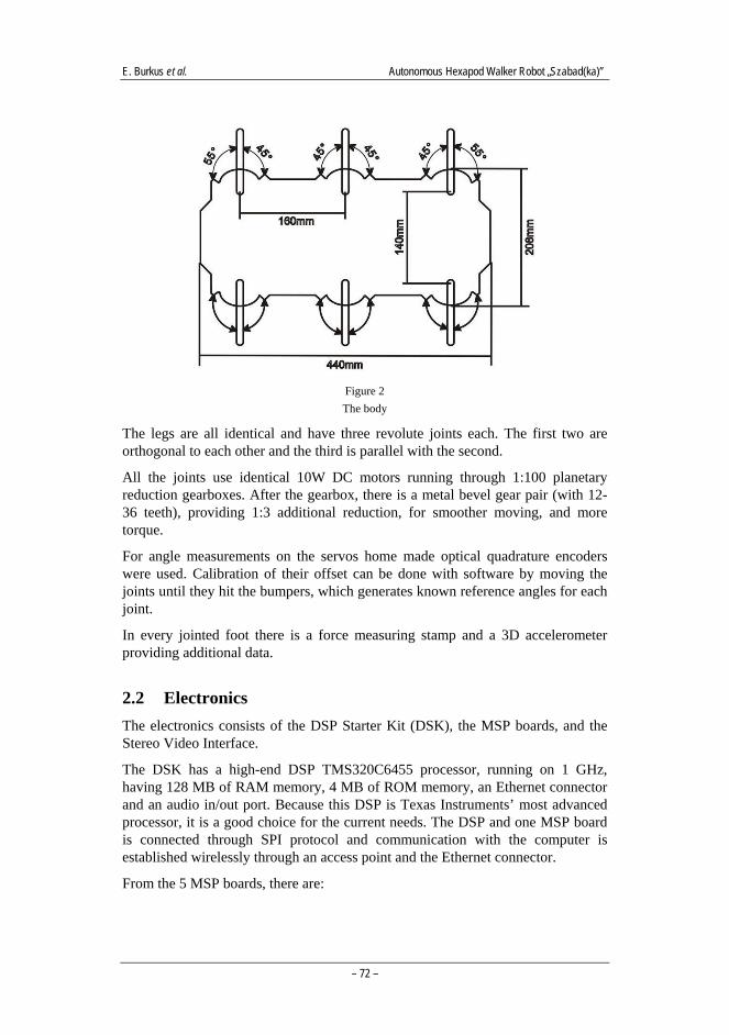
Figure 2 shows the body and the locations of the six identical legs with the approximate movements available about the α axis of each leg before they hit the bumpers on the chassis.

The leg attachments all lie in the same plane, with all the α axes parallel. Besides holding the legs, the function of the chassis is to hold the electronics and the accumulator, too.


– 72 –

Figure 2 The body

The legs are all identical and have three revolute joints each. The first two are orthogonal to each other and the third is parallel with the second.

All the joints use identical 10W DC motors running through 1:100 planetary reduction gearboxes. After the gearbox, there is a metal bevel gear pair (with 12-36 teeth), providing 1:3 additional reduction, for smoother moving, and more torque.

For angle measurements on the servos home made optical quadrature encoders were used. Calibration of their offset can be done with software by moving the joints until they hit the bumpers, which generates known reference angles for each joint.

In every jointed foot there is a force measuring stamp and a 3D accelerometer providing additional data.

2.2 Electronics The electronics consists of the DSP Starter Kit (DSK), the MSP boards, and the Stereo Video Interface.

The DSK has a high-end DSP TMS320C6455 processor, running on 1 GHz, having 128 MB of RAM memory, 4 MB of ROM memory, an Ethernet connector and an audio in/out port. Because this DSP is Texas Instruments’ most advanced processor, it is a good choice for the current needs. The DSP and one MSP board is connected through SPI protocol and communication with the computer is established wirelessly through an access point and the Ethernet connector.

From the 5 MSP boards, there are:


– 73 –

- 1 Sensors board

- 1 Communications – Motion Algorithm board, and

- 3 Inverse Kinematics boards.

The Communications – Motion Algorithm board, contains 2 MSP processors. One of them is the one, which is connected to the DSP processor. Its main tasks are to transceivers the commands between the DSP and the other MSP-s, and to generate the walking coordinates in dependence of time. The other MSP’s job is to process the rear gyroscopes, the rear accelerometers, and some infra red collision signals.

The task of the 3 Inverse Kinematics boards is to receive the coordinates from the Communications – Motion Algorithm board and to generate the desired angles of 3 joints for a leg. Logically, every IK board has 2 MSP-s, one for each leg. This board’s other task is to process the data received from the force sensors and the accelerometers placed in the feet.

The Sensors board’s first MSP controls the 2 ultra sound radars (it moves RC servo motors, and processes data), and the second MSP's job is to process the front gyroscopes, the front accelerometers, and some infra red collision signals.

The Stereo Video Interface connects 2 digital, high resolution cameras with the DSP-s EMIF (External Memory Interface). This board contains a FIFO memory. This is needed because the camera is sending its video data continuously and slowly, but the DSP can read data only rapidly, and in smaller parts. Because of the current special needs, the Digital Camera boards are also home made, using OV7640 video IC-s.

2.3 Software The robot’s software is physically divided into 3 parts. These are: the software running on the PC, the DSP software, and the MSP software.

For the PC, currently there is some controlling software written in JAVA, and a MATLAB platform. Both of them are capable for moving the robot in various directions, with various speeds, and with other options. The JAVA software is also prepared for receiving video data and other information from the robot. Further, it can set some behaviour.

About the DSP software: currently its only task is to transmit data between the PC and the Communication MSP but it will be used for image processing and decision making as soon the Stereo Video Interface will be finished. Some contour recognition and other algorithms are already written for it, and ready to use. The DSP software is written in C++ with Code Composer Studio.

The tasks of the software on the 5 MSP boards (on the 10 MSP controllers) were already described under the electronics section, thus 6 MSP-s are for Inverse


– 74 –

Kinematics, 2 MSP-s are processing one gyroscope, one accelerometer, and some IR sensors (per each controller), 1 MSP is for controlling, and processing 2 US radars, and 1 MSP is for communications, and for motion algorithms.

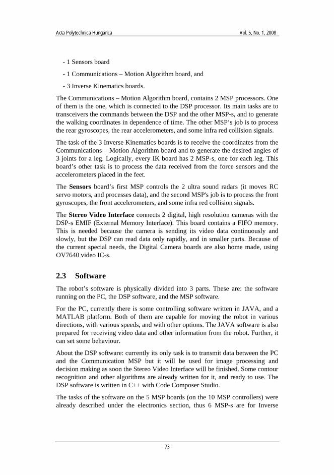
2.4 Animation In order for our calculation results to be visualized more easily, without a implementing or using the robot, we created an animation ‘subsystem’.

Figure 3

MATLAB simulation for one leg

A 3D Studio Max robot model, which is able to create an animation, based on data from imported using Matlab generated databases containing movement data. This procedure produced good results, but its drawback is that it needs an outside program (outside of Matlab), therefore the animation is not real-time.

So as to fix this problem we started to develop an ‘animation system’ within Simulink environment. With this we are currently able to visualize an animation within a Matlab environment, and are currently working on making it real-time. Figure 3 shows a detail of the robot’s MATLAB Simulink animation.

3 Robot Geometry Calculations The following section will present several explanatory drawings which illustrate the geometrical calculations.

The first mechanical drawing (Figure 4) shows how many degrees the joints can turn compared to their starting point. Figures 5 and 6 will help to define the maximum tilt angles of the joints. Fig. 6 shows the basic state assumed at the DK (direct kinematics) and IK (inverse kinematics) calculations. The ‘difference angles’ used in calculations is shown in Figure 7.


– 75 –

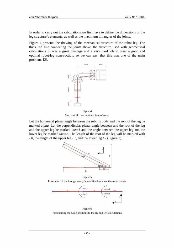
In order to carry out the calculations we first have to define the dimensions of the leg structure’s elements, as well as the maximum tilt angles of the joints.

Figure 4 presents the drawing of the mechanical structure of the robot leg. The thick red line connecting the joints shows the structure used with geometrical calculations. It was a great challege and a very hard job to creat a good and optimal robot-leg construction, so we can say, that this was one of the main problems [2].

Figure 4

Mechanical construction a foot of robot

Let the horizontal planar angle between the robot’s body and the root of the leg be marked alpha. Let the perpendicular planar angle between and the root of the leg and the upper leg be marked theta1 and the angle between the upper leg and the lower leg be marked theta2. The length of the root of the leg will be marked with L0, the length of the upper leg L1, and the lower leg L2 (Figure 7).

Figure 5

Illustration of the foot geometry`s modification when the robot moves

Figure 6

Presentating the basic positions to the IK and DK calculations


– 76 –

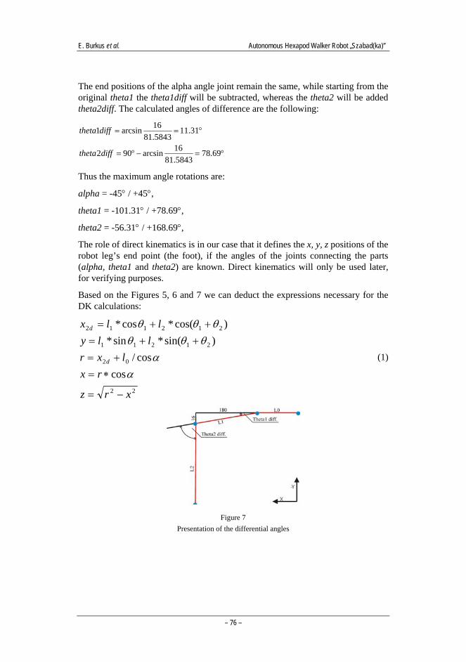
The end positions of the alpha angle joint remain the same, while starting from the original theta1 the theta1diff will be subtracted, whereas the theta2 will be added theta2diff. The calculated angles of difference are the following:

°=−°=

°==

69.785843.8116arcsin902

31.115843.8116arcsin1

difftheta

difftheta

Thus the maximum angle rotations are:

alpha = -45° / +45°,

theta1 = -101.31° / +78.69°,

theta2 = -56.31° / +168.69°,

The role of direct kinematics is in our case that it defines the x, y, z positions of the robot leg’s end point (the foot), if the angles of the joints connecting the parts (alpha, theta1 and theta2) are known. Direct kinematics will only be used later, for verifying purposes.

Based on the Figures 5, 6 and 7 we can deduct the expressions necessary for the DK calculations:

22

02

21211

212112

coscos/

)sin(*sin*)cos(*cos*

xrz

rxlxr

llyllx

d

d

−=

∗=+=

++=++=

αα

θθθθθθ

(1)

Figure 7

Presentation of the differential angles


– 77 –

4 Calculation of the Course of the Robot’s Foot We were looking for the numerically simplest solutions during the initial phase of development. The aim of this minimization was for the robot to be able to walk on a given course. The aim in this phase was not to include complex controlling conditions, which implement the signals of the sensors of the several accelerometers, gyroscopes, etc.

The calculations for the movement of the flat base of the foot can be put into three groups:

- first the course of the base of the foot in general is described using spline. A certain value will be given to the variable in this expression for the course, depending on how many points the wished course is to be converged to.

- the second calculation the coordinates thus received will help us calculate the necessary angle shift, i.e. we carry out the IK calculation.

- the third calculation refers to the operation of the motors helping the foot’s movement using PID controller.

4.1 Calculation of the Leg’s Trajectory In a general case for the description of the current position of the robot foot the Hermite cubic spline calculation method is used for given points P1, P4 and tangent vectors R1, R4. Look at x component:

( ) xxxx dtctbtatx +++= 23 (2)

So want to solve for ax, bx, cx and dx using the four continuity conditions, i.e. for two curve segments there is C0 and C1 continuity. So we have: x(0) = P1x, x(1) = P4x , x'(0) = R1x, x'(1) = R4x, end form of eqution is for x:

)()2()32()132()( 234

231

234

231 ttRtttRttPttPtx xxxx −++−++−++−= (3)

with similar expressions for y, z coordinats.

The use of spline calculation method for the description of foot movement is a great advantage if the ground is not even or there are obstacles on the ground. But in the realization of initial movement this is not the goal, but only to realize the simplest walk algorithm.

The number of operations is shown in Table 1 broken down according to the type of operations.

In the initial phase of robot development the aim was to use the simplest possible algorithms in the realization. In this simple case the 3D foot movement can be broken down to two functional parts:


– 78 –

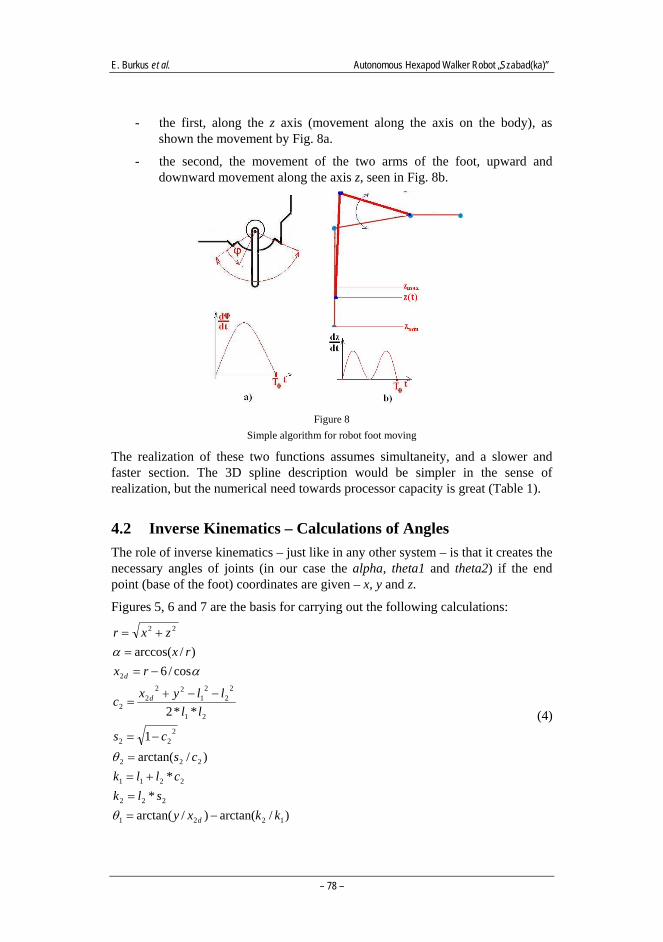
- the first, along the z axis (movement along the axis on the body), as shown the movement by Fig. 8a.

- the second, the movement of the two arms of the foot, upward and downward movement along the axis z, seen in Fig. 8b.

Figure 8

Simple algorithm for robot foot moving

The realization of these two functions assumes simultaneity, and a slower and faster section. The 3D spline description would be simpler in the sense of realization, but the numerical need towards processor capacity is great (Table 1).

4.2 Inverse Kinematics – Calculations of Angles The role of inverse kinematics – just like in any other system – is that it creates the necessary angles of joints (in our case the alpha, theta1 and theta2) if the end point (base of the foot) coordinates are given – x, y and z.

Figures 5, 6 and 7 are the basis for carrying out the following calculations:

)/arctan()/arctan(*

*)/arctan(

1

**2

cos/6)/arccos(

1221

222

2211

222

222

21

22

21

222

2

2

22

kkxyslk

cllkcs

cs

llllyxc

rxrx

zxr

d

d

d

−==

+==

−=

−−+=

−==

+=

θ

θ

αα

(4)


– 79 –

4.3 Numerical Calculations with Microcontrollers The 6 inverse kinematics calculations necessary for the movement of the feet (one for each foot) are carried out by a microcontroller.

The section will discuss the numerical needs of the kinematics calculations for moving the 3 DOF robot legs using a 8 MHz clock signal 16-bit inner architecture microcontroller from the MSP430F16xx family. This microcontroller family is of fix point arithmetic structure and has a 16-bit parallel multiplier.

The MSP1612 was used because it has a 16-bit parallel multiplier and a low consumption, as well as the highest number of operations (performance) index among microcontrollers.

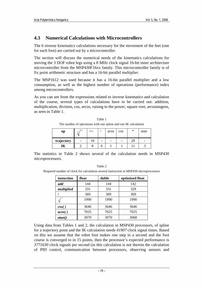
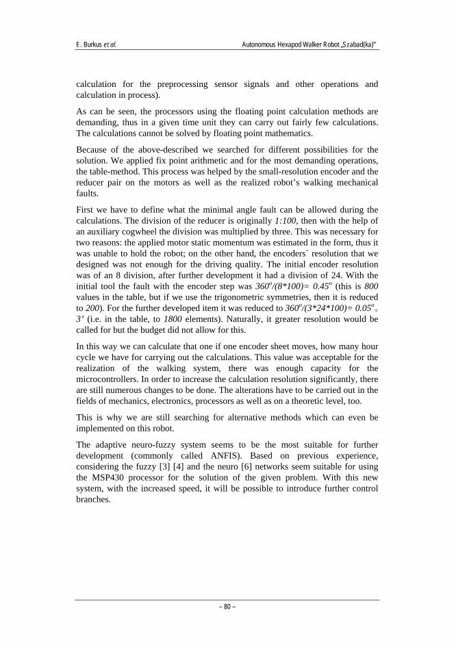
As you can see from the expressions related to inverse kinematics and calculation of the course, several types of calculations have to be carried out: addition, multiplication, division, cos, arcos, raising to the power, square root, arcustangens, as seen in Table 1.

Table 1 The number of operations with one spline and one IK calculation

op 2 +/- / acos cos * atan

trajectory - 10 - - - 29 - IK 2 8 6 1 1 11 3

The statistics in Table 2 shows several of the calculation needs in MSP430 microprocessors.

Table 2 Required number of clock for calculation several instruction in MSP430 microprocessors

instuction float duble optimised float add 144 144 142 multiplied 331 331 329 / 369 369 369 2 1990 1990 1990

cos( ) 3646 3646 3646 acos( ) 7025 7025 7025 atan() 3070 3070 3068

Using data from Tables 1 and 2, the calculation in MSP430 processors, of spline for a trajectory point and the IK calculation needs 41907 clock signal times. Based on this we assume that the robot foot makes one step in a second and the foot course is converged to in 15 points, then the processor’s expected performance is 3771630 clock signals per second (in this calculation is not therein the calculation of PID control, communication between processors, observing sensors and


– 80 –

calculation for the preprocessing sensor signals and other operations and calculation in process).

As can be seen, the processors using the floating point calculation methods are demanding, thus in a given time unit they can carry out fairly few calculations. The calculations cannot be solved by floating point mathematics.

Because of the above-described we searched for different possibilities for the solution. We applied fix point arithmetic and for the most demanding operations, the table-method. This process was helped by the small-resolution encoder and the reducer pair on the motors as well as the realized robot’s walking mechanical faults.

First we have to define what the minimal angle fault can be allowed during the calculations. The division of the reducer is originally 1:100, then with the help of an auxiliary cogwheel the division was multiplied by three. This was necessary for two reasons: the applied motor static momentum was estimated in the form, thus it was unable to hold the robot; on the other hand, the encoders` resolution that we designed was not enough for the driving quality. The initial encoder resolution was of an 8 division, after further development it had a division of 24. With the initial tool the fault with the encoder step was 360o/(8*100)= 0.45o (this is 800 values in the table, but if we use the trigonometric symmetries, then it is reduced to 200). For the further developed item it was reduced to 360o/(3*24*100)= 0.05o

= 3’ (i.e. in the table, to 1800 elements). Naturally, it greater resolution would be called for but the budget did not allow for this.

In this way we can calculate that one if one encoder sheet moves, how many hour cycle we have for carrying out the calculations. This value was acceptable for the realization of the walking system, there was enough capacity for the microcontrollers. In order to increase the calculation resolution significantly, there are still numerous changes to be done. The alterations have to be carried out in the fields of mechanics, electronics, processors as well as on a theoretic level, too.

This is why we are still searching for alternative methods which can even be implemented on this robot.

The adaptive neuro-fuzzy system seems to be the most suitable for further development (commonly called ANFIS). Based on previous experience, considering the fuzzy [3] [4] and the neuro [6] networks seem suitable for using the MSP430 processor for the solution of the given problem. With this new system, with the increased speed, it will be possible to introduce further control branches.


– 81 –

5 ANFIS ANFIS method is a hybrid neuro-fuzzy technique that brings learning capabilities of neural networks to fuzzy inference systems [5]. The learning algorithm in adaptive neural technique tunes the membership functions of a Sugeno-type Fuzzy Inference System using the training input-output data. In our case, the input data is coordinate dataset and output data angles dataset. The learning-training algorithm ANFIS map the co-ordinates to the angles.

With the help of Fuzzy logic we create a Fuzzy interference system which is able to conclude the inverse kinematics; if the task’s forward kinematics is known.

Since the forward kinematics of the three-degrees-freedom robot foot is known, the base foot’s x, y and z coordinates can be defined for the entire domain of the three joints’ angles. The coordinates and their respective angles are stored for the training of our ANFIS network.

During the process of training the ANFIS systems learns how to pair up the coordinates (x,y,z) with the angles (alpha, theta1, theta2). The trained ANFIS network is thus capable of interference the joint angles based on the required position of the base foot.

The next section will turn to the presentation of MATLAB implementation. In the future course of research the robot will be implemented in a multiprocessor environment.

5.1 Creation of Input Data The x, y and z coordinates are defined for alpha, theta1 and theta2 in all structurally possible combinations with the given resolution, using forward kinematics (1). The results are stored in three columns:

data1 (x, y, z, alpha),

data2 (x, y, z, theta1),

data3 (x, y, z, theta2).

5.2 Building the ANFIS Network For the ANFIS system solution we have to create 3 ANFIS networks.

For the ANFIS network to be able to predict the necessary angles, first it has to be trained with the suitable input and output data. The first ANFIS network will be trained for x, y, z input data and alpha output data. The previously created data1 matrix contains the necessary x,y,z – alpha data set.


– 82 –

Similarly, the second ANFIS network will be trained for the x,y,z-theta1 data set stored in the data2 matrix, whereas the third ANFIS network will be trained for the x,y,z-theta2 stored in the data3 matrix. In the current situation we can train the ANFIS network with MATLAB anfis function. If the function is requested with a simple syntax, it automatically creates a Sugeno-type FIS, and trains it with the given data.

anfis1 = anfis(data1, 6, 150, [0,0,0,0]); % train first ANFIS network

anfis2 = anfis(data2, 6, 150, [0,0,0,0]); % train second ANFIS network

anfis3 = anfis(data3, 6, 150, [0,0,0,0]); % train third ANFIS network

The first parameter of ANFIS is the training data, the second the number of membership functions, the third is the number of epochs. In order to reach the right exactness, the number of membership functions and the epochs can be defined after several attempts.

After the training anfis1, anfis2, and anfis3 represent the three trained ANFIS networks. After the training is finished, the 3 ANFIS networks have to be able to approximately define the output angles based on the x, y and z input functions. One of the advantages of the fuzzy approach is tat the ANFIS network is able to define even such angles that do not match with, only bear similarity with the angles used in training. With the help of the network we can define the angles of those points which are found between two points, found in the practice table.

5.3 Control of the ANFIS Network After the training of the network another important task is to verify our network, to find out how precisely our ANFIS network is able to converge to the results of inverse kinematics. Since in our case we know the inverse kinematics deductions, there is no obstacle to doing this.

We have to generate a 3D matrix which contains the coordinates x, y and z with the given resolution for points of the chosen work space. After this we define the angles alpha, theta1 and theta2 for the given points using inverse kinematics (4):

THREE blocks: data1, data2, data3

In the following step with the help of the trained network we define their angles using the same coordinates. In the end the gained results are compared and we can see how close the FIS outputs are to the results of our inverse kinematics.

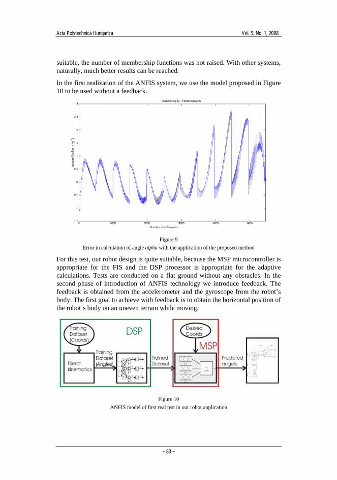
Figure 9 shows the error in the calculation of angle α with the application of the proposed method for 3 fuzzy membership functions, the accumulated error already with 3 membership functions within the error limit of the robot mechanics. By the increase of membership functions we could receive better results, but since the key factor in our system is the decrease of calculation time, and the preciseness is


– 83 –

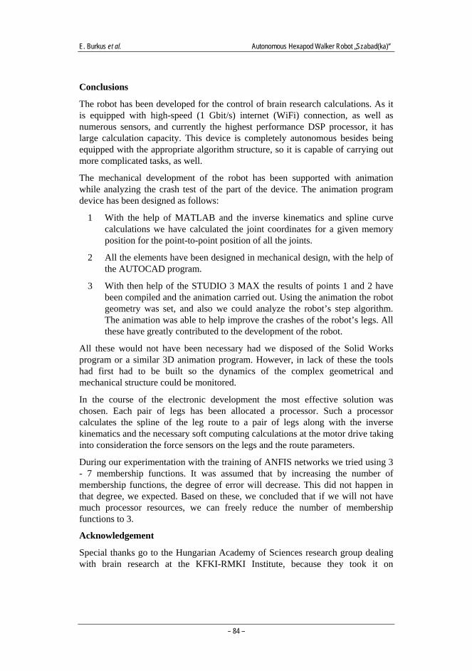
suitable, the number of membership functions was not raised. With other systems, naturally, much better results can be reached. In the first realization of the ANFIS system, we use the model proposed in Figure 10 to be used without a feedback.

Figure 9

Error in calculation of angle alpha with the application of the proposed method

For this test, our robot design is quite suitable, because the MSP microcontroller is appropriate for the FIS and the DSP processor is appropriate for the adaptive calculations. Tests are conducted on a flat ground without any obstacles. In the second phase of introduction of ANFIS technology we introduce feedback. The feedback is obtained from the accelerometer and the gyroscope from the robot’s body. The first goal to achieve with feedback is to obtain the horizontal position of the robot’s body on an uneven terrain while moving.

Figure 10

ANFIS model of first real test in our robot application


– 84 –

Conclusions

The robot has been developed for the control of brain research calculations. As it is equipped with high-speed (1 Gbit/s) internet (WiFi) connection, as well as numerous sensors, and currently the highest performance DSP processor, it has large calculation capacity. This device is completely autonomous besides being equipped with the appropriate algorithm structure, so it is capable of carrying out more complicated tasks, as well.

The mechanical development of the robot has been supported with animation while analyzing the crash test of the part of the device. The animation program device has been designed as follows:

1 With the help of MATLAB and the inverse kinematics and spline curve calculations we have calculated the joint coordinates for a given memory position for the point-to-point position of all the joints.

2 All the elements have been designed in mechanical design, with the help of the AUTOCAD program.

3 With then help of the STUDIO 3 MAX the results of points 1 and 2 have been compiled and the animation carried out. Using the animation the robot geometry was set, and also we could analyze the robot’s step algorithm. The animation was able to help improve the crashes of the robot’s legs. All these have greatly contributed to the development of the robot.

All these would not have been necessary had we disposed of the Solid Works program or a similar 3D animation program. However, in lack of these the tools had first had to be built so the dynamics of the complex geometrical and mechanical structure could be monitored.

In the course of the electronic development the most effective solution was chosen. Each pair of legs has been allocated a processor. Such a processor calculates the spline of the leg route to a pair of legs along with the inverse kinematics and the necessary soft computing calculations at the motor drive taking into consideration the force sensors on the legs and the route parameters.

During our experimentation with the training of ANFIS networks we tried using 3 - 7 membership functions. It was assumed that by increasing the number of membership functions, the degree of error will decrease. This did not happen in that degree, we expected. Based on these, we concluded that if we will not have much processor resources, we can freely reduce the number of membership functions to 3.

Acknowledgement

Special thanks go to the Hungarian Academy of Sciences research group dealing with brain research at the KFKI-RMKI Institute, because they took it on


– 85 –

themselves to finance this robot and continually monitor our activities around the development of the robot.

We are also grateful to the College of Dunaújváros for having agreed to carry out the robot’s etch work using CNC. The development of the robot has furthermore been supported by Zsolt Takács from Subotica and the Gordos family from Ada with their work and advice.

Thanks for Tibor Szakáll helps in calculating the necessary processor aqusition times for trigonometric and algebric calculations.

We have to say thank you for Péter Dukán, Mihály Klosák and Árpád Miklós who have helped us in the final operation of the robot project.

References

[1] M. R. Fielding, R. Dunlop, C. J. Damaren: Hamlet: Force/Position controlled Hexapod Walker – Design and Systems, Proc. IEEE Int. Conf. of Controll Appl., Mexico, 2001, pp. 984-989

[2] P. Gonzales de Santos, E. Garcia, J. Estremera: Improving Walking-Robot Performances by Optimizing Leg Distribution, Auton. Robot, Vol. 23, 2007, pp. 247-258

[3] Odry Péter et. al.: ‘Fuzzy Logic Motor Control with MSP430x14x’, Application Report, Texas Instruments, (SLAA 235), February 2005

[4] Péter Odry, Szabolcs Divéki, Nándor Búrány, László Gyantár: ‘Fuzzy Control of Brush Motor - Problems of Computing’, Plenary section, invited paper, SISY 2004, Subotica, pp. 37-46, ISBN 963 7154 32 9

[5] Jyh-Shing Roger Jang: ANFIS: Adaptive-Network-based Fuzzy Inference System, IEEE Trans. on Systems, Man and Cibernetics, Vol. 23, No. 3, May/June 1993, pp. 665-685

[6] Péter Odry, Gábor Kávai: ‘Neural Motor Control’, SISY 2005, Subotica, pp. 15-21, ISBN 963 7154 418

Documents

Autonomous Hexapod Walker Robot “Szabad(ka)”uni-obuda.hu/journal/Burkus_Odry_13.pdf“Szabad(ka)” Ervin Burkus, Peter Odry ... The robot’s weight is 1.5 kg. ... The robot’s