Automated Refinement Checking of Concurrent

Systems

Sudipta Kundu Sorin Lerner Rajesh Gupta

University of California, San Diego

La Jolla, CA 92093-0404

Email: {skundu, lerner, rgupta}@cs.ucsd.edu

August 2007

Abstract

Stepwise refinement is at the core of many approaches to synthesisand optimization of hardware and software systems. For instance, it canbe used to build a synthesis approach for digital circuits from high levelspecifications. It can also be used for post-synthesis modification such asin Engineering Change Orders (ECOs). Therefore, checking if a system,modeled as a set of concurrent processes, is a refinement of another is oftremendous value. In this paper, we focus on concurrent systems modeledas Communicating Sequential Processes (CSP) and show their refinementscan be validated using insights from translation validation, automatedtheorem proving and relational approaches to reasoning about programs.The novelty of our approach is that it handles infinite state spaces in afully automated manner. We have implemented our refinement checkingtechnique and have applied it to a variety of refinements. We present thedetails of our algorithm and experimental results. As an example, we wereable to automatically check an infinite state space buffer refinement thatcannot be checked by current state of the art tools such as FDR. We werealso able to check the data part of an industrial case study on the EP2system.

1 Introduction

Growing complexity of systems and their implementation into Silicon encour-ages designers to look for ways to model designs at higher levels of abstrac-tion and then incrementally build portions of these designs – automatically ormanually – while ensuring system-level functional correctness [6]. For instance,researchers have advocated the use of SystemC models and their stepwise refine-ment into interacting hardware and software components [24]. At the heart of

1

such proposals is a model of the system consisting of concurrent pieces of func-tionality, oftentimes expressed as sequential program-like behavior, along withsynchronous or asynchronous interactions [23, 37]. Communicating SequentialProcesses [18] (CSP) is a calculus for describing such concurrent systems as a setof processes that communicate synchronously over explicitly named channels.

Refinement checking of CSP programs consists of checking that, once a re-finement has been performed, the resulting refined design, expressed as a CSPprogram, is indeed a correct refinement of the original high-level design, alsoexpressed as a CSP program. Broadly speaking, refinements are useful becausethey provide guarantees about the two programs that are in the refinement re-lation. Many notions of refinement exist, for example trace refinement, failuresrefinement, or failures/divergence refinement [35]. Each kind of refinement pro-vides its own guarantees. For example, trace refinement preserves safety proper-ties, failures refinement also preserves liveness properties and deadlock freedom,and failures/divergence refinement also preserves livelock freedom [35].

Refinement checking of CSP programs has many applications. As one ex-ample, Allen and Garlen have shown how CSP programs can be used as typesto describe the interfaces of software components [3]. The refinement relationbecomes a sub-typing relation, and refinement checking can then be used to de-termine if two components, whose interfaces are specified using CSP programs,are compatible.

Another important application of refinement checking appears in the contextof refinement-based software or hardware design [38]. The engineer starts with ahigh-level description of the design, usually called a specification, which is thencontinually refined into more and more concrete implementations. Checkingcorrectness of these refinement steps has many benefits, including finding bugsin the refinements, while at the same time guaranteeing that properties checkedat higher-levels in the design are preserved through the refinement process,without having to recheck them at lower levels. For example, if one checks thata given specification satisfies a safety property, and that an implementation is acorrect trace refinement of the specification, then the implementation will alsosatisfy the safety property.

Refinement checking of CSP programs is an area that has been widely ex-plored. However, as we will explain in further detail throughout the rest of thepaper, previous work on CSP refinement falls into two broad categories. First,there has been research on techniques that require human assistance. Thiswork ranges from completely manual proof techniques, such as Josephs’s workon relational approaches to CSP refinement checking [20], to semi-automatedtechniques where humans must provide hints to guide a theorem prover in check-ing refinements [13, 39, 19, 27, 28, 29]. Second, there has been work on fullyautomated techniques to CSP refinement checking [2, 10], the state of the artbeing embodied in the FDR tool [2]. These techniques essentially perform an ex-haustive state space exploration, which places onerous restrictions on the kindsof infinite state spaces they can handle. In particular, they can only handleone kind of infinite state space, namely those arising from data-independentprograms. Such programs must treat the data they process as black boxes, and

2

the only operation they can do on data is to copy it. Although there has beenwork on making the finite state spaces that automated techniques can handlelarger and larger [7, 11, 33, 36], there has been little work on automaticallyhandling refinement checking of two concurrent programs whose state spacesare truly infinite. This is a serious limitation when attempting to raise the levelof abstraction of system models to move beyond the bit-oriented data structuresused in RTL specifications.

In this paper we present a new trace refinement checking algorithm for CSPprograms. Our algorithm uses a simulation relation approach to proving refine-ment. In particular, we automatically establish a simulation relation that stateswhat points in the specification program are related to what points in the im-plementation program. This simulation relation guarantees that for each tracein the implementation, a related and equivalent trace exists in the specification.Although there has been work on using simulation relations for automaticallychecking concurrent systems in a fully automated way, their use has been focusedon specific low-level hardware refinements [25, 26].

Our algorithm consists of two components. The first component is given asimulation relation, and checks that this relation satisfies the properties requiredfor it to be a correct refinement simulation relation. The second componentautomatically infers a simulation relation just from the specification and theimplementation programs. Once the simulation relation is inferred, it can thenbe checked for correctness using the checking algorithm.

Unlike previous approaches, our approach can automatically check the re-finement of infinite state space CSP programs that are not data-independent.This means that we can handle CSP programs that manipulate, inspect, andbranch on data ranging over truly infinite domains, for example the set of allintegers or all reals. In order to achieve this additional checking power, our al-gorithm draws insights and techniques from various areas, including translationvalidation [34, 30], theorem proving [12], and relational approaches to reason-ing about programs [20, 22]. As a result, the contribution of our paper can beseen in different lights. One way to characterize our contribution is that wehave automated a previously known, but completely manual technique, namelyJosephs’s relational approach to proving CSP refinements [20]. Another way tocharacterize our contribution is that we have incorporated an automated theo-rem proving component to FDR’s search technique [2] in order to handle infinitestate spaces that are not data-independent. Yet another way to characterize ourcontribution is that we have generalized translation validation [34, 30], an au-tomated technique for checking that two sequential programs are equivalent, toaccount for concurrency and for trace containment checking.

To evaluate our approach, we used the Simplify theorem prover [12] to im-plement our CSP refinement checking algorithms in a validating system calledARCCoS (Automated Refinement Checker for Concurrent Systems). We thenused our implementation to check the correctness of a variety of refinements,including parts of an industrial case study of the EP2 system [1].

The remainder of the paper is organized as follows. Section 2 presents anoverview of our approach, and shows how our algorithm works on a simple

3

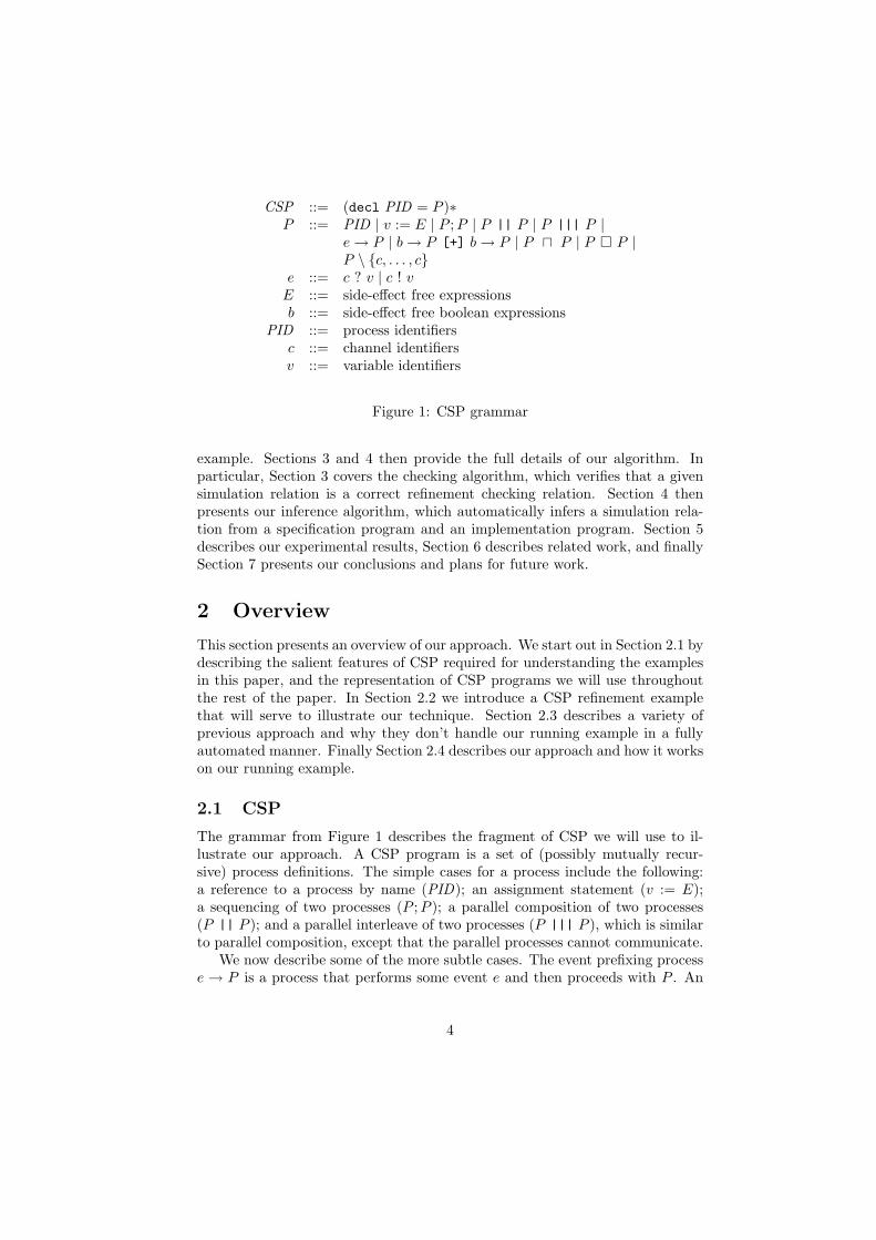
CSP ::= (decl PID = P )∗P ::= PID | v := E | P ;P | P || P | P ||| P |

e→ P | b→ P [+] b→ P | P ⊓ P | P � P |P \ {c, . . . , c}

e ::= c ? v | c ! vE ::= side-effect free expressionsb ::= side-effect free boolean expressions

PID ::= process identifiersc ::= channel identifiersv ::= variable identifiers

Figure 1: CSP grammar

example. Sections 3 and 4 then provide the full details of our algorithm. Inparticular, Section 3 covers the checking algorithm, which verifies that a givensimulation relation is a correct refinement checking relation. Section 4 thenpresents our inference algorithm, which automatically infers a simulation rela-tion from a specification program and an implementation program. Section 5describes our experimental results, Section 6 describes related work, and finallySection 7 presents our conclusions and plans for future work.

2 Overview

This section presents an overview of our approach. We start out in Section 2.1 bydescribing the salient features of CSP required for understanding the examplesin this paper, and the representation of CSP programs we will use throughoutthe rest of the paper. In Section 2.2 we introduce a CSP refinement examplethat will serve to illustrate our technique. Section 2.3 describes a variety ofprevious approach and why they don’t handle our running example in a fullyautomated manner. Finally Section 2.4 describes our approach and how it workson our running example.

2.1 CSP

The grammar from Figure 1 describes the fragment of CSP we will use to il-lustrate our approach. A CSP program is a set of (possibly mutually recur-sive) process definitions. The simple cases for a process include the following:a reference to a process by name (PID); an assignment statement (v := E);a sequencing of two processes (P ;P ); a parallel composition of two processes(P || P ); and a parallel interleave of two processes (P ||| P ), which is similarto parallel composition, except that the parallel processes cannot communicate.

We now describe some of the more subtle cases. The event prefixing processe → P is a process that performs some event e and then proceeds with P . An

4

event e can either be reading a value from a channel c into a variable v (c?v),or writing a variable v to a channel c (c!v). Reads and writes are synchronous.

The case statement b1 → P1 [+] b2 → P2 executes P1 or P2 based on whichof the two boolean conditions b1 or b2 is true. If both are true, the choice is madenon-deterministically. If neither is true, the statement can’t make progress.

The non-deterministic choice process P1 ⊓ P2 executes either P1 or P2 non-deterministically.

The external choice process P1�P2 executes either P1 or P2 depending onwhat events the surrounding environment is willing to engage in. For example(c1?v → P1)�(c2?v → P2) will execute the left or right side of the � operatordepending on what channel (c1 or c2) first has a value. If both channels havea value, then the choice is made non-deterministically. The external choiceoperator resembles the select system call in Unix and Linux systems.

The channel hiding process P \ {c1, . . . , cn} acts like P but hides all theevents that occur on channels c1, . . . , cn. Channels that are not hidden areexternally visible, and these are the channels that we preserve the behavior ofwhen checking refinement.

Parallel processes in our version of CSP (and Hoare’s original version too)can only communicate through messages on channels. Although there are noexplicit shared variables, these can easily be simulated using a process thatstores the value of the shared variable, and that services reads and writes to thevariable using messages.

As an example, here is a simple CSP program:

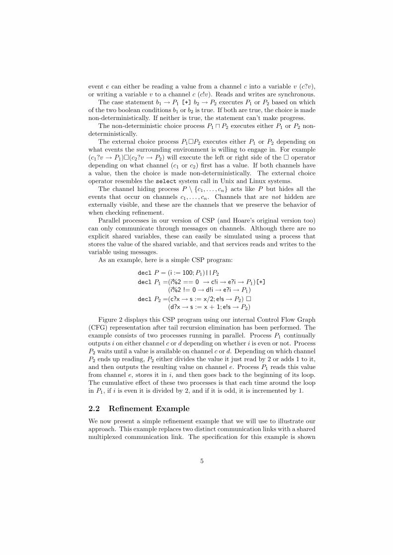
decl P = (i := 100;P1)||P2

decl P1 =(i%2 == 0 → c!i → e?i → P1)[+](i%2 != 0 → d!i → e?i → P1)

decl P2 =(c?x → s := x/2; e!s → P2) �

(d?x → s := x + 1; e!s → P2)

Figure 2 displays this CSP program using our internal Control Flow Graph(CFG) representation after tail recursion elimination has been performed. Theexample consists of two processes running in parallel. Process P1 continuallyoutputs i on either channel c or d depending on whether i is even or not. ProcessP2 waits until a value is available on channel c or d. Depending on which channelP2 ends up reading, P2 either divides the value it just read by 2 or adds 1 to it,and then outputs the resulting value on channel e. Process P1 reads this valuefrom channel e, stores it in i, and then goes back to the beginning of its loop.The cumulative effect of these two processes is that each time around the loopin P1, if i is even it is divided by 2, and if it is odd, it is incremented by 1.

2.2 Refinement Example

We now present a simple refinement example that we will use to illustrate ourapproach. This example replaces two distinct communication links with a sharedmultiplexed communication link. The specification for this example is shown

5

i := 100

[+]

i%2==0 i%2!=0

d ! ic ! i

e ? i

| |

c ? x d ? x

s:=x+1s:=x/2

e ! s

P1 P2

e ? i e ! s

Figure 2: Example CFG representation of a CSP program

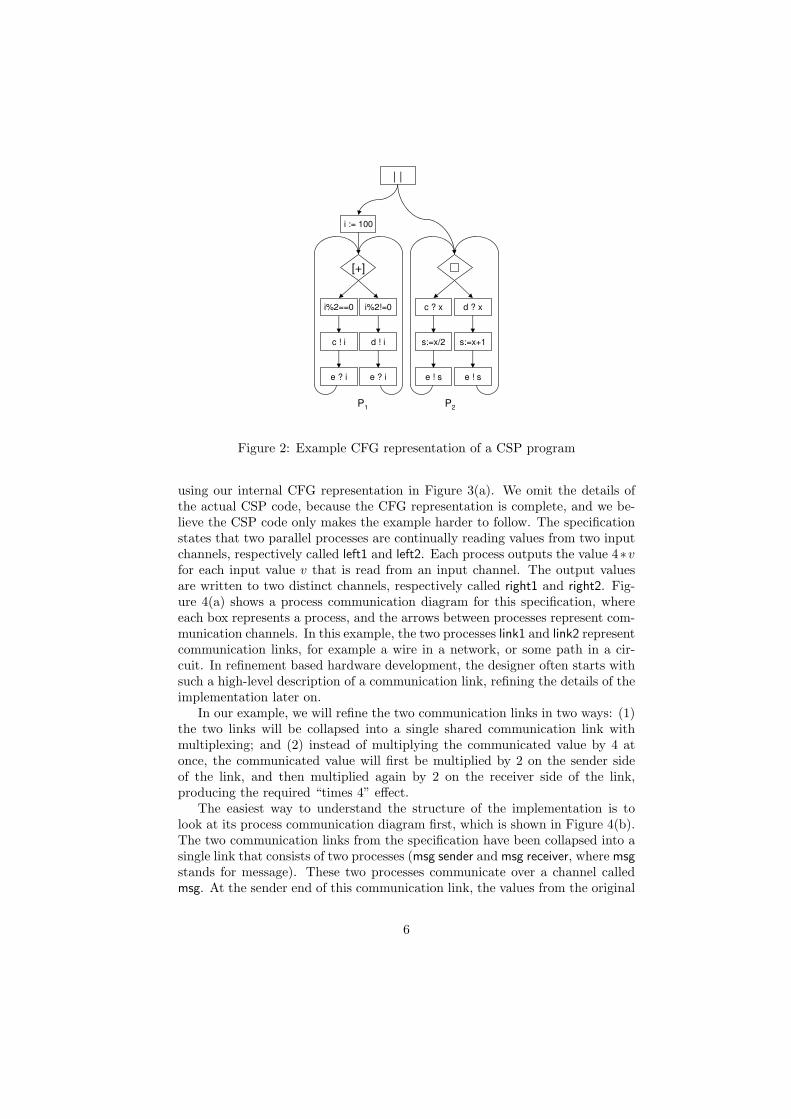
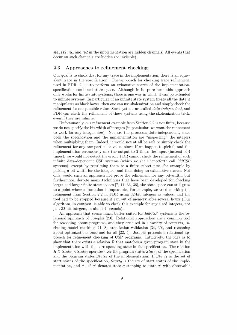
using our internal CFG representation in Figure 3(a). We omit the details ofthe actual CSP code, because the CFG representation is complete, and we be-lieve the CSP code only makes the example harder to follow. The specificationstates that two parallel processes are continually reading values from two inputchannels, respectively called left1 and left2. Each process outputs the value 4∗vfor each input value v that is read from an input channel. The output valuesare written to two distinct channels, respectively called right1 and right2. Fig-ure 4(a) shows a process communication diagram for this specification, whereeach box represents a process, and the arrows between processes represent com-munication channels. In this example, the two processes link1 and link2 representcommunication links, for example a wire in a network, or some path in a cir-cuit. In refinement based hardware development, the designer often starts withsuch a high-level description of a communication link, refining the details of theimplementation later on.

In our example, we will refine the two communication links in two ways: (1)the two links will be collapsed into a single shared communication link withmultiplexing; and (2) instead of multiplying the communicated value by 4 atonce, the communicated value will first be multiplied by 2 on the sender sideof the link, and then multiplied again by 2 on the receiver side of the link,producing the required “times 4” effect.

The easiest way to understand the structure of the implementation is tolook at its process communication diagram first, which is shown in Figure 4(b).The two communication links from the specification have been collapsed into asingle link that consists of two processes (msg sender and msg receiver, where msgstands for message). These two processes communicate over a channel calledmsg. At the sender end of this communication link, the values from the original

6

sm2?y

z := y*2

sm1?x

z:=x*2

msg!1 msg!2

msg!zmsg!z

j==2

ra2!1

j==1

ra1!1

[+]

ack?j

| | |

sa2?_

ack!2

sa1?_

ack!1

i==2

rm2!p

i==1

rm1!p

[+]

msg?i

p:=q*2

| | |

msg?q

| | |

sm2!b

ra2?_

left1?a

sm1!a

ra1?_

left2?b

| | |

right2!r

sa2!1

rm1?s

right1!s

sa1!1

rm2?r

| |

leftlink1

leftlink2

msgsender

ackreceiver

msgreceiver

acksender

rightlink1

rightlink2

| |

z:=b*4

right2!z

left1?a

w:=a*4

right1!w

left2?b

link1 link2

(b) Implementation(a) Specification

Figure 3: CFGs for the specification and implementation of our running example

leftlink1

left1

leftlink2

left2

msgsender

ackreceiver

msgreceiver

acksender

rightlink1

right1

rightlink2

right2

msg

ack

sm1

sm2

ra2

ra1

rm1

sa1

sa2

rm2

shared communicationlink for messages

shared communicationlink for acks

link1left1 right1

link2left2 right2

communication link 2

communication link 1

(b) Implementation(a) Specification

Figure 4: Process communication diagram for the specification and implemen-tation of our running example

Name Line type Condition

A

B

Spec.a == Impl.a

Spec.w == Impl.s

Figure 5: Sample entries from the simulation relation

7

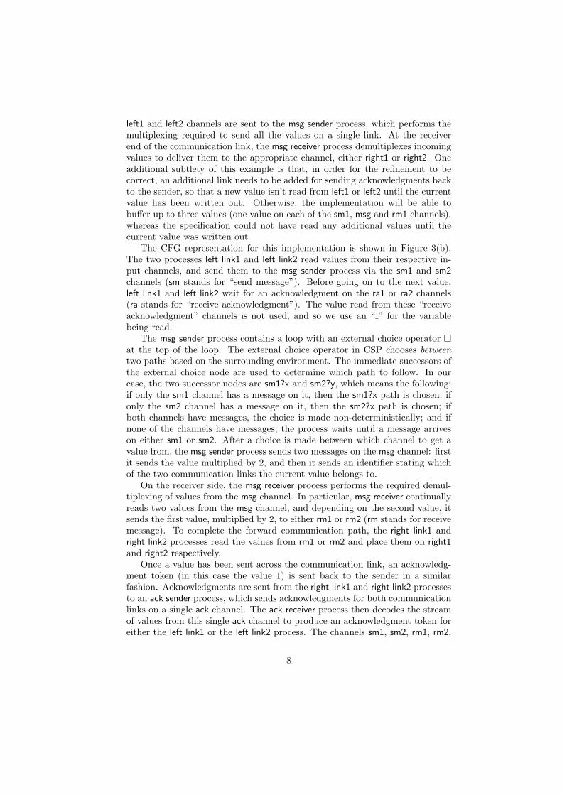
left1 and left2 channels are sent to the msg sender process, which performs themultiplexing required to send all the values on a single link. At the receiverend of the communication link, the msg receiver process demultiplexes incomingvalues to deliver them to the appropriate channel, either right1 or right2. Oneadditional subtlety of this example is that, in order for the refinement to becorrect, an additional link needs to be added for sending acknowledgments backto the sender, so that a new value isn’t read from left1 or left2 until the currentvalue has been written out. Otherwise, the implementation will be able tobuffer up to three values (one value on each of the sm1, msg and rm1 channels),whereas the specification could not have read any additional values until thecurrent value was written out.

The CFG representation for this implementation is shown in Figure 3(b).The two processes left link1 and left link2 read values from their respective in-put channels, and send them to the msg sender process via the sm1 and sm2channels (sm stands for “send message”). Before going on to the next value,left link1 and left link2 wait for an acknowledgment on the ra1 or ra2 channels(ra stands for “receive acknowledgment”). The value read from these “receiveacknowledgment” channels is not used, and so we use an “ ” for the variablebeing read.

The msg sender process contains a loop with an external choice operator �

at the top of the loop. The external choice operator in CSP chooses betweentwo paths based on the surrounding environment. The immediate successors ofthe external choice node are used to determine which path to follow. In ourcase, the two successor nodes are sm1?x and sm2?y, which means the following:if only the sm1 channel has a message on it, then the sm1?x path is chosen; ifonly the sm2 channel has a message on it, then the sm2?x path is chosen; ifboth channels have messages, the choice is made non-deterministically; and ifnone of the channels have messages, the process waits until a message arriveson either sm1 or sm2. After a choice is made between which channel to get avalue from, the msg sender process sends two messages on the msg channel: firstit sends the value multiplied by 2, and then it sends an identifier stating whichof the two communication links the current value belongs to.

On the receiver side, the msg receiver process performs the required demul-tiplexing of values from the msg channel. In particular, msg receiver continuallyreads two values from the msg channel, and depending on the second value, itsends the first value, multiplied by 2, to either rm1 or rm2 (rm stands for receivemessage). To complete the forward communication path, the right link1 andright link2 processes read the values from rm1 or rm2 and place them on right1and right2 respectively.

Once a value has been sent across the communication link, an acknowledg-ment token (in this case the value 1) is sent back to the sender in a similarfashion. Acknowledgments are sent from the right link1 and right link2 processesto an ack sender process, which sends acknowledgments for both communicationlinks on a single ack channel. The ack receiver process then decodes the streamof values from this single ack channel to produce an acknowledgment token foreither the left link1 or the left link2 process. The channels sm1, sm2, rm1, rm2,

8

sa1, sa2, ra1 and ra2 in the implementation are hidden channels. All events thatoccur on such channels are hidden (or invisible).

2.3 Approaches to refinement checking

Our goal is to check that for any trace in the implementation, there is an equiv-alent trace in the specification. One approach for checking trace refinement,used in FDR [2], is to perform an exhaustive search of the implementation-specification combined state space. Although in its pure form this approachonly works for finite state systems, there is one way in which it can be extendedto infinite systems. In particular, if an infinite state system treats all the data itmanipulates as black boxes, then one can use skolemization and simply check therefinement for one possible value. Such systems are called data-independent, andFDR can check the refinement of these systems using the skolemization trick,even if they are infinite.

Unfortunately, our refinement example from Section 2.2 is not finite, becausewe do not specify the bit-width of integers (in particular, we want the refinementto work for any integer size). Nor are the processes data-independent, sinceboth the specification and the implementation are “inspecting” the integerswhen multiplying them. Indeed, it would not at all be safe to simply check therefinement for any one particular value, since, if we happen to pick 0, and theimplementation erroneously sets the output to 2 times the input (instead of 4times), we would not detect the error. FDR cannot check the refinement of suchinfinite data-dependent CSP systems (which we shall henceforth call IddCSPsystems), except by restricting them to a finite subset first, for example bypicking a bit-width for the integers, and then doing an exhaustive search. Notonly would such an approach not prove the refinement for any bit-width, butfurthermore, despite many techniques that have been developed for checkinglarger and larger finite state spaces [7, 11, 33, 36], the state space can still growto a point where automation is impossible. For example, we tried checking therefinement from Section 2.2 in FDR using 32-bit integers as values, and thetool had to be stopped because it ran out of memory after several hours (Ouralgorithm, in contrast, is able to check this example for any sized integers, notjust 32-bit integers, in about 4 seconds).

An approach that seems much better suited for IddCSP systems is the re-lational approach of Josephs [20]. Relational approaches are a common toolfor reasoning about programs, and they are used in a variety of contexts, in-cluding model checking [21, 8], translation validation [34, 30], and reasoningabout optimizations once and for all [22, 5]. Josephs presents a relational ap-proach for refinement checking of CSP programs. Intuitively, the idea is toshow that there exists a relation R that matches a given program state in theimplementation with the corresponding state in the specification. The relationR ⊆ S tate1×S tate2 operates over the program states S tate1 of the specificationand the program states S tate2 of the implementation. If S tart1 is the set ofstart states of the specification, S tart2 is the set of start states of the imple-mentation, and σ →e σ′ denotes state σ stepping to state σ′ with observable

9

events e, then the following conditions summarize Josephs requirements for acorrect refinement:

∀σ2 ∈ S tart2 . ∃σ1 ∈ S tart1 . R(σ1, σ2)∀σ1 ∈ S tate1, σ2 ∈ S tate2, σ

′2∈ S tate2 .

σ2 →e σ′2∧R(σ1, σ2) ⇒

∃σ′1∈ S tate1 . σ1 →e σ′

1∧R(σ′

1, σ′

2)

These conditions respectively state that (1) for each starting state in the im-plementation, there must be a related state in the specification; and (2) if thespecification and the implementation are in a pair of related states, and theimplementation can proceed to produce observable events e, then the specifica-tion must also be able to proceed, producing the same events e, and the tworesulting states must be related. The above conditions are the base case andthe inductive case of a proof by induction showing that the implementation isa trace refinement of the specification.

Although Josephs’s approach can handle IddCSP systems, automating hisapproach turns out to be difficult for two reasons. First, the patterns of quan-tifiers that appear in the above conditions confuse the heuristics of state of theart theorem provers such as Simplify [12], and as a result, it seems unlikely thata theorem prover could prove the above conditions directly, without any hu-man assistance. Second, to use Josephs’s relational approach, one has to comeup with a candidate relation to begin with, something that Josephs does notaddress in his work.

More generally, there has been little work on checking trace refinement (andother refinements too) of two truly infinite CSP systems in a completely auto-matic way. Various tools have been developed for reasoning about such CSPsystems [13, 39, 19], using a variety of theorem provers [31, 32]. But all thesetools are interactive in nature, and they require some sort of human assistance,usually in the form of a proof script that states which theorem proving tacticsshould be applied to perform the proof.

Although not directly in the context of CSP, there has been work on check-ing refinement of concurrent systems, for example in the context of the MAGICtool [9]. However, our approach is different from MAGIC’s counter-exampledriven approach, and it is also considerably simpler. We show that our seem-ingly simple approach, which was inspired by Necula’s work on translation val-idation [30], in fact works well in practice.

2.4 Our approach

Our technique for refinement checking builds on Josephs’s relational approachby overcoming the difficulties of automation with a simple division-of-labor ap-proach. In particular, we handle infinite state spaces by splitting the state spaceinto two parts: the control flow state, which is finite, and the dataflow state,which may be infinite. The exploration of the control flow state is done usinga specialized algorithm that traverses our internal CFG representation of CSPprograms. Along paths discovered by the control flow exploration, the dataflow

10

state is explored using an automated theorem prover. Although this way ofsplitting the state space has previously been used in reasoning about a givensequential program [15, 17, 4, 14], a given concurrent program [9], or a pair ofsequential programs [34, 30], its use in reasoning about the refinement of twoinfinite state space concurrent programs is novel.

Our approach consists of two parts, which theoretically are independent,but for practical reasons, we have made one part subsume the other. The firstpart is a checking algorithm that, given a relation, determines whether or not itsatisfies the properties required for it to be a valid refinement-checking relation.The second part is an inference algorithm that infers a relation given two CSPprograms, one of which is a specification, and one of which is an implementation.To check that one CSP program is a refinement of another, one therefore runs theinference algorithm to infer a relation, and then one uses the checking algorithmto verify that the resulting relation is indeed a refinement-checking relation.However, because the inference algorithm does a similar kind of exploration asthe checking algorithm, this leads to a lot of duplicate work. To address thisissue, we have made the inference algorithm also perform checking, with onlya small amount of additional work. This avoids having the checking algorithmduplicate the exploration work done by the inference algorithm. The checkingalgorithm is nonetheless useful by itself, in case our inference algorithm is notcapable of finding an appropriate relation, and a human wants to provide therelation by hand.

2.4.1 Simulation Relation

The goal of the simulation relation in our approach is to guarantee that the spec-ification and the implementation interact in the same way with any surroundingenvironment that they would be placed in.

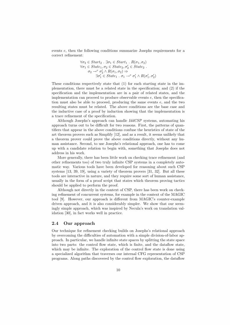
The simulation relation in our algorithm consists of a set of entries of theform (p1, p2, φ), where p1 and p2 are program points in the specification andimplementation respectively, and φ is a boolean formula over variables of thespecification and implementation. The pair (p1, p2) captures how the controlstate of the specification is related to the control state of the implementation,whereas φ captures how the data is related. As an example, Figure 3 pictoriallyshows two simulation relation entries. We use lines to represent the controlcomponent of entries in the simulation relation by connecting all the nodes inthe CFG that belong to the entry being represented (the actual program pointthat belongs to the entry is the program point right before the node). The datacomponent of these two entries are given in Figure 5.

The first entry in Figure 3, shown with a dashed line and labeled A inFigure 5, shows the specification just as it finishes reading a value from theleft1 channel. The corresponding control state of the implementation has theleft link1 process in the same state, just as it finishes reading from the left1channel. The msg sender process in the implementation at this point has alreadychosen the sm1?x branch of its external choice � operator, since the left link1process is about to execute a write to the sm1 channel. All other processes in

11

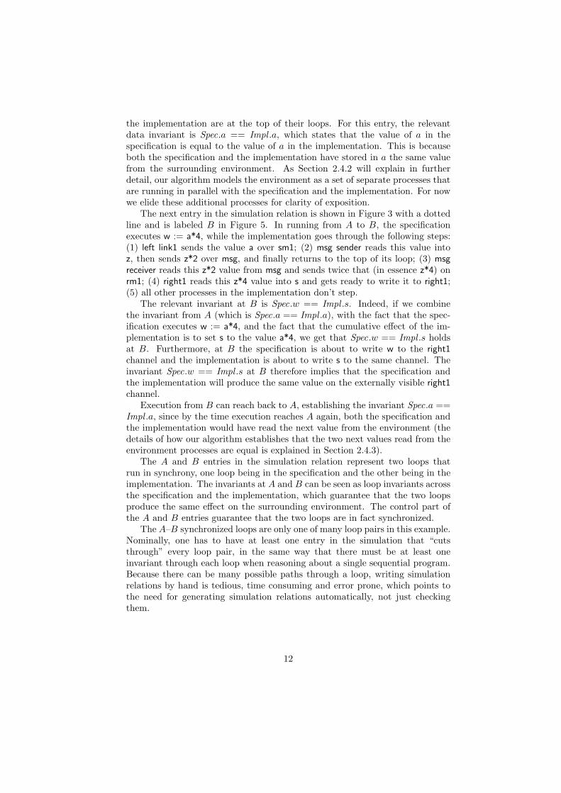
the implementation are at the top of their loops. For this entry, the relevantdata invariant is Spec.a == Impl .a, which states that the value of a in thespecification is equal to the value of a in the implementation. This is becauseboth the specification and the implementation have stored in a the same valuefrom the surrounding environment. As Section 2.4.2 will explain in furtherdetail, our algorithm models the environment as a set of separate processes thatare running in parallel with the specification and the implementation. For nowwe elide these additional processes for clarity of exposition.

The next entry in the simulation relation is shown in Figure 3 with a dottedline and is labeled B in Figure 5. In running from A to B, the specificationexecutes w := a*4, while the implementation goes through the following steps:(1) left link1 sends the value a over sm1; (2) msg sender reads this value intoz, then sends z*2 over msg, and finally returns to the top of its loop; (3) msgreceiver reads this z*2 value from msg and sends twice that (in essence z*4) onrm1; (4) right1 reads this z*4 value into s and gets ready to write it to right1;(5) all other processes in the implementation don’t step.

The relevant invariant at B is Spec.w == Impl .s. Indeed, if we combinethe invariant from A (which is Spec.a == Impl .a), with the fact that the spec-ification executes w := a*4, and the fact that the cumulative effect of the im-plementation is to set s to the value a*4, we get that Spec.w == Impl .s holdsat B. Furthermore, at B the specification is about to write w to the right1channel and the implementation is about to write s to the same channel. Theinvariant Spec.w == Impl .s at B therefore implies that the specification andthe implementation will produce the same value on the externally visible right1channel.

Execution from B can reach back to A, establishing the invariant Spec.a ==Impl .a, since by the time execution reaches A again, both the specification andthe implementation would have read the next value from the environment (thedetails of how our algorithm establishes that the two next values read from theenvironment processes are equal is explained in Section 2.4.3).

The A and B entries in the simulation relation represent two loops thatrun in synchrony, one loop being in the specification and the other being in theimplementation. The invariants at A and B can be seen as loop invariants acrossthe specification and the implementation, which guarantee that the two loopsproduce the same effect on the surrounding environment. The control part ofthe A and B entries guarantee that the two loops are in fact synchronized.

The A–B synchronized loops are only one of many loop pairs in this example.Nominally, one has to have at least one entry in the simulation that “cutsthrough” every loop pair, in the same way that there must be at least oneinvariant through each loop when reasoning about a single sequential program.Because there can be many possible paths through a loop, writing simulationrelations by hand is tedious, time consuming and error prone, which points tothe need for generating simulation relations automatically, not just checkingthem.

12

2.4.2 Checking Algorithm

Given a simulation relation, our checking algorithm checks each entry in therelation individually. For each entry (p1, p2, φ), it finds all other entries thatare reachable from (p1, p2), without going through any intermediary entries.For each such entry (p′

1, p′

2, ψ), we check using a theorem prover that if (1) φ

holds at p1 and p2, (2) the specification executes from p1 to p′1

and (3) theimplementation executes from p2 to p′

2, then ψ will hold at p′

1and p′

2.

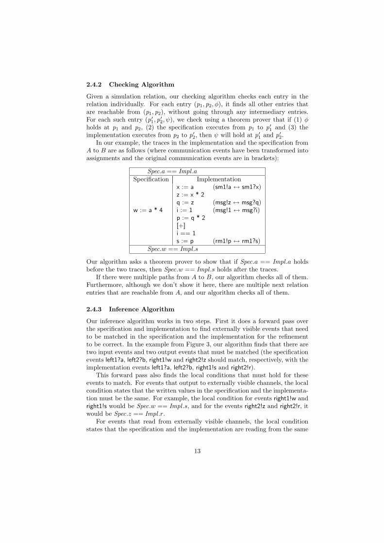
In our example, the traces in the implementation and the specification fromA to B are as follows (where communication events have been transformed intoassignments and the original communication events are in brackets):

Spec.a == Impl .aSpecification Implementation

x := a (sm1!a ↔ sm1?x)z := x * 2q := z (msg!z ↔ msg?q)

w := a * 4 i := 1 (msg!1 ↔ msg?i)p := q * 2[+]i == 1s := p (rm1!p ↔ rm1?s)

Spec.w == Impl .s

Our algorithm asks a theorem prover to show that if Spec.a == Impl .a holdsbefore the two traces, then Spec.w == Impl .s holds after the traces.

If there were multiple paths from A to B, our algorithm checks all of them.Furthermore, although we don’t show it here, there are multiple next relationentries that are reachable from A, and our algorithm checks all of them.

2.4.3 Inference Algorithm

Our inference algorithm works in two steps. First it does a forward pass overthe specification and implementation to find externally visible events that needto be matched in the specification and the implementation for the refinementto be correct. In the example from Figure 3, our algorithm finds that there aretwo input events and two output events that must be matched (the specificationevents left1?a, left2?b, right1!w and right2!z should match, respectively, with theimplementation events left1?a, left2?b, right1!s and right2!r).

This forward pass also finds the local conditions that must hold for theseevents to match. For events that output to externally visible channels, the localcondition states that the written values in the specification and the implementa-tion must be the same. For example, the local condition for events right1!w andright1!s would be Spec.w == Impl .s, and for the events right2!z and right2!r, itwould be Spec.z == Impl .r.

For events that read from externally visible channels, the local conditionstates that the specification and the implementation are reading from the same

13

point in the conceptual stream of input values. To achieve this, we use anautomatically generated environment process that models each externally vis-ible input channel c as an unbounded array values of input values, with anindex variable i stating which value in the array should be read next. Thisenvironment process runs an infinite loop that continually outputs values[i]to c and increments i. Assuming that i and j are the index variables fromthe environment processes that model an externally visible channel c in thespecification and the implementation, respectively, then the local conditionfor matching events c?a (in the specification) and c?b (in the implementa-tion) would then be Spec.i == Impl .j. The equality between the index vari-ables implies that the values being read are the same, and since this fact isalways true, we directly add it to the generated local condition, producingSpec.i == Impl .j ∧ Spec.a == Impl .b.

Once the first pass of our algorithm has found all matching events, and hasseeded all matching events with local conditions, the second pass or our algo-rithm propagates these local conditions backward through the specification andimplementation in parallel, using weakest preconditions. The final conditionscomputed by this weakest-precondition propagation make up the simulation re-lation. Because of loops, we must iterate to a fixed point, and although ingeneral this procedure may not terminate, in practice it can quickly find therequired simulation relation.

We use weakest preconditions to infer the simulation relation rather thanstrongest postconditions because the weakest precondition approach is moregoal directed: we start with the seed conditions we want to hold, and then onlycompute the conditions required to establish these seeds. In contrast, doingstrongest postconditions in the forward direction would compute everythingthat is derivable at a given program point, which would cause our algorithmto often compute facts that are not relevant, and as a result diverge. To seethe difference, consider for example a specification and an implementation thatboth have loops incrementing a variable i and outputting each value of i onan externally visible channel. The strongest post-condition approach on thisexample would basically be tantamount to running the program, and would notterminate. On the other hand, the weakest precondition approach, if seededwith Spec.i == Impl .i (since those are the values sent on the externally visiblechannel) would appropriately find out that the invariant is Spec.i == Impl .i.Our work in fact confirms Necula’s finding in his translation validation work [30]that a weakest precondition approach to inferring simulation relations works wellin practice.

3 Checking Algorithm

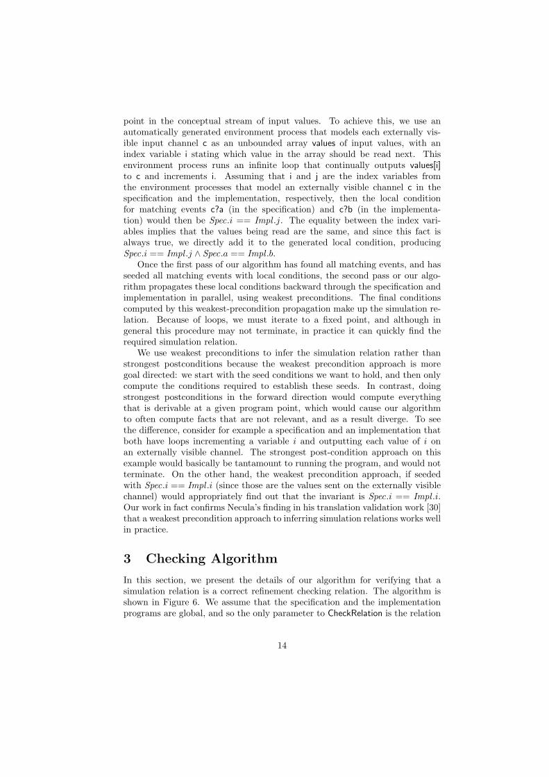
In this section, we present the details of our algorithm for verifying that asimulation relation is a correct refinement checking relation. The algorithm isshown in Figure 6. We assume that the specification and the implementationprograms are global, and so the only parameter to CheckRelation is the relation

14

1. procedure CheckRelation(R : VerificationRelation)2. for each (p1, p2, φ) ∈ R do

3. if ¬Explore([p1], [p2], φ,R) then

4. Error(“Trace in Impl not found in Spec”)5. let (Seeds , ) := ComputeSeeds()6. CheckImplication(R,Seeds)

7. function Explore(t1 : Trace, t2 : Trace, φ : Formula,8. R : VerificationRelation) : Boolean9. for each p2 such that t2 → p2 do

10. let found := false11. for each p1 such that t1 → p1 do

12. if ¬IsInfeasible(t1 :: p1, t2 :: p2, φ) then

13. if ∃i > 0 . t1[i] = p1 ∧ t2[i] = p2 then

14. Warning(“Loop with no relation entry”)15. elseif ∃ψ . (p1, p2, ψ) ∈ R then

16. found := true17. PreImpliesPost(φ, t1 :: p1, t2 :: p2, ψ)18. else

19. if Explore(t1 :: p1, t2 :: p2, φ,R) then

20. found := true21. if ¬found then

22. return false23. return true

24. procedure PreImpliesPost(φ : Formula, t1 : Trace,25. t2 : Trace, ψ : Formula)26. let ψ′ := wp(t1,wp(t2, ψ))27. if ATP(φ⇒ ψ′) 6= Valid then

28. Error(“Cannot verify relation entry”)

Figure 6: Algorithm for checking a simulation relation

15

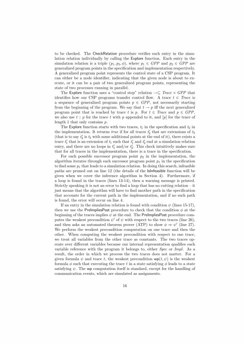
to be checked. The CheckRelation procedure verifies each entry in the simu-lation relation individually by calling the Explore function. Each entry in thesimulation relation is a triple (p1, p2, φ), where p1 ∈ GPP and p2 ∈ GPP aregeneralized program points in the specification and implementation respectively.A generalized program point represents the control state of a CSP program. Itcan either be a node identifier, indicating that the given node is about to ex-ecute, or it can be a pair of two generalized program points, representing thestate of two processes running in parallel.

The Explore function uses a “control step” relation →⊆ Trace × GPP thatidentifies how our CSP programs transfer control flow. A trace t ∈ Trace isa sequence of generalized program points p ∈ GPP , not necessarily startingfrom the beginning of the program. We say that t → p iff the next generalizedprogram point that is reached by trace t is p. For t ∈ Trace and p ∈ GPP ,we also use t :: p for the trace t with p appended to it, and [p] for the trace oflength 1 that only contains p.

The Explore function starts with two traces, t1 in the specification and t2 inthe implementation. It returns true if for all traces t ′

2that are extensions of t2

(that is to say t ′2

is t2 with some additional points at the end of it), there exists atrace t ′

1that is an extension of t1 such that t ′

1and t ′

2end at a simulation relation

entry, and there are no loops in t ′1

and/or t ′2. This check intuitively makes sure

that for all traces in the implementation, there is a trace in the specification.For each possible successor program point p2 in the implementation, the

algorithm iterates through each successor program point p1 in the specificationto find some p1 that leads to a simulation relation. In doing this search, infeasiblepaths are pruned out on line 12 (the details of the IsInfeasible function will begiven when we cover the inference algorithm in Section 4). Furthermore, ifa loop is found in the traces (lines 13-14), then a warning message is printed.Strictly speaking it is not an error to find a loop that has no cutting relation – itjust means that the algorithm will have to find another path in the specificationthat accounts for the current path in the implementation, and if no such pathis found, the error will occur on line 4.

If an entry in the simulation relation is found with condition ψ (lines 15-17),then we use the PreImpliesPost procedure to check that the condition φ at thebeginning of the traces implies ψ at the end. The PreImpliesPost procedure com-putes the weakest precondition ψ′ of ψ with respect to the two traces (line 26),and then asks an automated theorem prover (ATP) to show φ ⇒ ψ′ (line 27).We perform the weakest precondition computation on one trace and then theother. When computing the weakest precondition with respect to one trace,we treat all variables from the other trace as constants. The two traces op-erate over different variables because our internal representation qualifies eachvariable reference with the program it belongs to, either Spec or Impl . As aresult, the order in which we process the two traces does not matter. For agiven formula ψ and trace t , the weakest precondition wp(t , ψ) is the weakestformula φ such that executing the trace t in a state satisfying φ leads to a statesatisfying ψ. The wp computation itself is standard, except for the handling ofcommunication events, which are simulated as assignments.

16

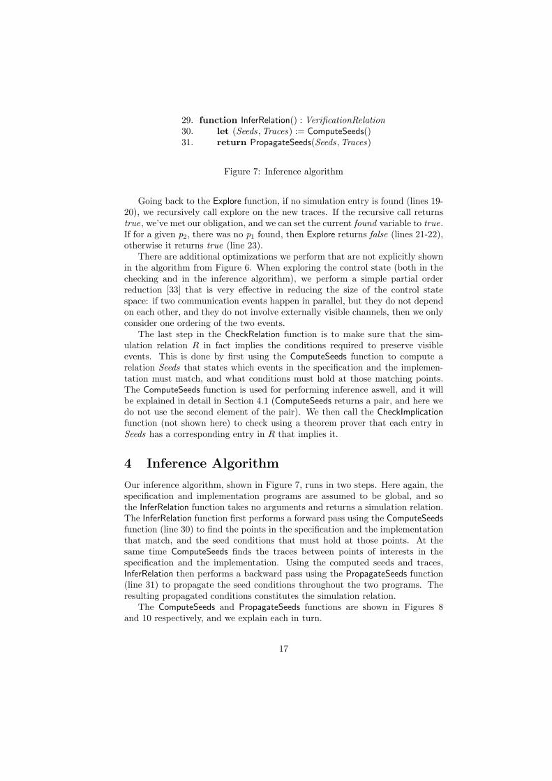
29. function InferRelation() : VerificationRelation30. let (Seeds ,Traces) := ComputeSeeds()31. return PropagateSeeds(Seeds ,Traces)

Figure 7: Inference algorithm

Going back to the Explore function, if no simulation entry is found (lines 19-20), we recursively call explore on the new traces. If the recursive call returnstrue, we’ve met our obligation, and we can set the current found variable to true.If for a given p2, there was no p1 found, then Explore returns false (lines 21-22),otherwise it returns true (line 23).

There are additional optimizations we perform that are not explicitly shownin the algorithm from Figure 6. When exploring the control state (both in thechecking and in the inference algorithm), we perform a simple partial orderreduction [33] that is very effective in reducing the size of the control statespace: if two communication events happen in parallel, but they do not dependon each other, and they do not involve externally visible channels, then we onlyconsider one ordering of the two events.

The last step in the CheckRelation function is to make sure that the sim-ulation relation R in fact implies the conditions required to preserve visibleevents. This is done by first using the ComputeSeeds function to compute arelation Seeds that states which events in the specification and the implemen-tation must match, and what conditions must hold at those matching points.The ComputeSeeds function is used for performing inference aswell, and it willbe explained in detail in Section 4.1 (ComputeSeeds returns a pair, and here wedo not use the second element of the pair). We then call the CheckImplicationfunction (not shown here) to check using a theorem prover that each entry inSeeds has a corresponding entry in R that implies it.

4 Inference Algorithm

Our inference algorithm, shown in Figure 7, runs in two steps. Here again, thespecification and implementation programs are assumed to be global, and sothe InferRelation function takes no arguments and returns a simulation relation.The InferRelation function first performs a forward pass using the ComputeSeedsfunction (line 30) to find the points in the specification and the implementationthat match, and the seed conditions that must hold at those points. At thesame time ComputeSeeds finds the traces between points of interests in thespecification and the implementation. Using the computed seeds and traces,InferRelation then performs a backward pass using the PropagateSeeds function(line 31) to propagate the seed conditions throughout the two programs. Theresulting propagated conditions constitutes the simulation relation.

The ComputeSeeds and PropagateSeeds functions are shown in Figures 8and 10 respectively, and we explain each in turn.

17

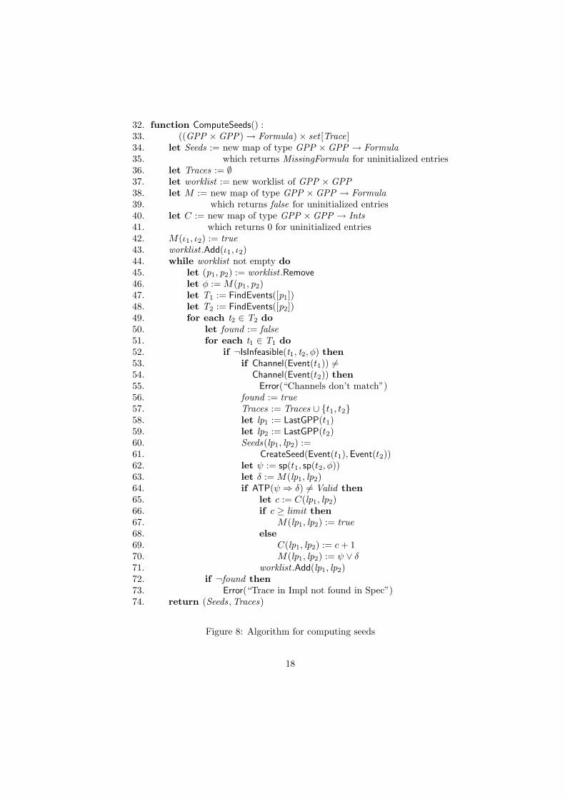
32. function ComputeSeeds() :33. ((GPP × GPP) → Formula) × set [Trace]34. let Seeds := new map of type GPP × GPP → Formula35. which returns MissingFormula for uninitialized entries36. let Traces := ∅37. let worklist := new worklist of GPP × GPP38. let M := new map of type GPP × GPP → Formula39. which returns false for uninitialized entries40. let C := new map of type GPP × GPP → Ints41. which returns 0 for uninitialized entries42. M(ι1, ι2) := true43. worklist .Add(ι1, ι2)44. while worklist not empty do

45. let (p1, p2) := worklist .Remove46. let φ := M(p1, p2)47. let T1 := FindEvents([p1])48. let T2 := FindEvents([p2])49. for each t2 ∈ T2 do

50. let found := false51. for each t1 ∈ T1 do

52. if ¬IsInfeasible(t1, t2, φ) then

53. if Channel(Event(t1)) 6=54. Channel(Event(t2)) then

55. Error(“Channels don’t match”)56. found := true57. Traces := Traces ∪ {t1, t2}58. let lp1 := LastGPP(t1)59. let lp2 := LastGPP(t2)60. Seeds(lp1, lp2) :=61. CreateSeed(Event(t1),Event(t2))62. let ψ := sp(t1, sp(t2, φ))63. let δ := M(lp1, lp2)64. if ATP(ψ ⇒ δ) 6= Valid then

65. let c := C(lp1, lp2)66. if c ≥ limit then

67. M(lp1, lp2) := true68. else

69. C(lp1, lp2) := c+ 170. M(lp1, lp2) := ψ ∨ δ71. worklist .Add(lp1, lp2)72. if ¬found then

73. Error(“Trace in Impl not found in Spec”)74. return (Seeds ,Traces)

Figure 8: Algorithm for computing seeds

18

75. function IsInfeasible(t1 : Trace, t2 : Trace,76. φ : Formula) : Boolean77. let ψ1 := sp(t1, φ)78. let ψ2 := sp(t2, φ)79. return ATP(¬(ψ1 ∧ ψ2)) = Valid

80. function FindEvents(t : Trace) : set [Trace]81. if VisibleEventOccurs(t) then

82. return {t}83. else

84. return⋃

t′∈{t::p|t→p}

FindEvents(t′)

Figure 9: Auxiliary functions

4.1 Computing Seeds

The ComputeSeeds function performs a forward pass over the specification andimplementation programs in synchrony to find externally visible events thatmust match. The algorithm maintains the following information:

• A map Seeds (lines 34-35) from generalized program point pairs (one programpoint in the specification and one in the implementation) to formulas. Thismap keeps track of discovered seeds.

• A set Traces (line 36) of discovered traces.

• A worklist (line 37) of generalized program point pairs.

• A map M (lines 38-39) from generalized program point pairs to a booleanformula approximating the set of the states that can appear at those programpoints. These formulas will be computed using strongest postconditions fromthe beginning of the specification and implementation programs, and will beused to find branch correlations between the implementation and the specifi-cation. The value returned by M for uninitialized entries is false, the mostoptimistic information.

• A map C (lines 40-41) from generalized program point pairs to an integerdescribing how many times each pair has been analyzed. Because propagat-ing strongest postconditions through loops may lead to an infinite chain offormulas at the loop entry, each weaker than the previous, we analyze eachprogram point pair at most limit times, where limit is a global parameter toour algorithm. After the limit is reached for a program point pair, its entryin M is set to true, the most conservative information, which guarantees thatit will never be analyzed again.

The ComputeSeeds algorithm starts by setting the value of M at the initialprogram points of the specification (ι1) and the implementation (ι2) to true,and adds (ι1, ι2) to the worklist. While the worklist is not empty, a generalized

19

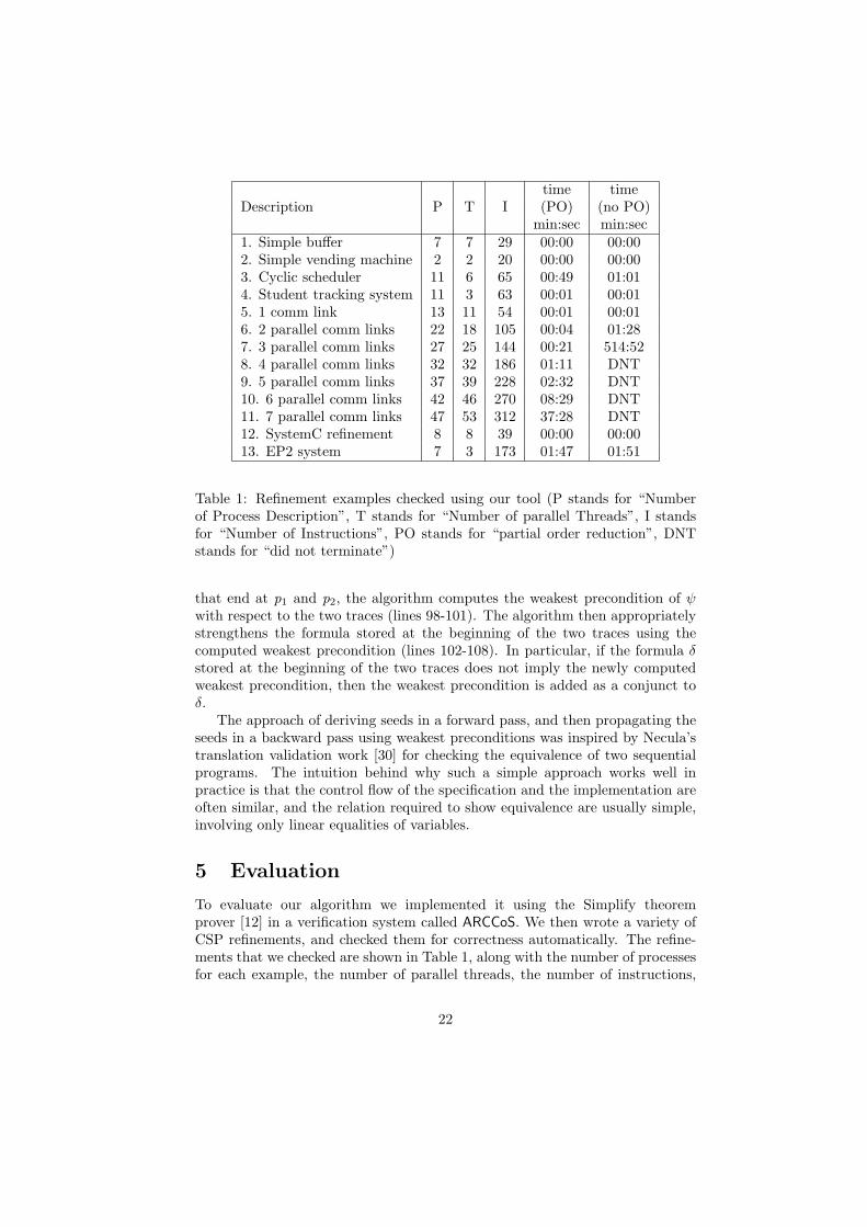
program pair (p1, p2) is removed from the worklist. Using an auxiliary functionFindEvents (see Figure 9), we find the set of all traces T1 that start at p1 andend at a communication event that is externally visible, and similarly for T2 (Acommunication event is externally visible if it occurs on a channel that is nothidden). For each t1 ∈ T1, and t2 ∈ T2, we check whether or not it is in factfeasible for the specification to follow t1 and the implementation to follow t2.The trace combination is infeasible if the strongest postconditions ψ1 and ψ2

of the two traces are inconsistent, which can be checked by asking a theoremprover to show ¬(ψ1 ∧ ψ2). This takes care of pruning within a single CSPprogram, but also across the specification and implementation.

Once we’ve identified that the two traces t1 and t2 may be a feasible combi-nation, we check that the events occurring at the end of these two traces are onthe same channel (lines 53-55). If they are not, then we have found an externallyvisible event that occurs in the implementation but not in the specification, andwe flag this as an error. If the events at the end of t1 and t2 occur on thesame channel, then we augment the Traces set with t1 and t2, and then weset the seed condition for the end points of the traces. The seed condition iscomputed by the CreateSeed function, not shown here. This function takes twocommunication events that involve an externally visible channel ext. Assumingthe two events are (ext!a ↔ ext?b) and (ext!c ↔ ext?d), the CreateSeed func-tion first checks if the communication involves reading from an automaticallygenerated environment process, in other words if the ext!a and ext!c instruc-tions belong to some environment processes. If so, then the generated seed isSpec.i == Impl .j ∧ Spec.b == Impl .d, where i and j are the index variables forthe automatically generated environment processes in the specification and im-plementation respectively (see Section 2.4.3 for a description of index variablesfor environment processes). If the communication does not involve reading froman environment process, then the seed is Spec.a == Impl .c.

The rest of the loop computes the strongest postcondition of the two traces t1and t2, and appropriately weakens the formula that approximates the run timestate at the end of the two traces. The first step is to compute the strongestpostcondition with respect to the trace t2 and then with respect to the trace t1using the sp function (line 62). For a given formula φ and trace t , the strongestpostcondition sp(t , φ) is the strongest formula ψ such that the if the statementsin the trace t are executed in sequence starting in a program state satisfying φ,then ψ will hold in the resulting program state. The sp computation itself isstandard, except for the handling of communication events, which are simulatedas assignments. Here again, the order in which we process the two traces doesnot matter.

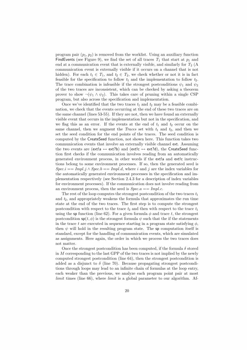
Once the strongest postcondition has been computed, if the formula δ storedinM corresponding to the last GPP of the two traces is not implied by the newlycomputed strongest postcondition (line 64), then the strongest postcondition isadded as a disjunct to δ (line 70). Because propagating strongest postcondi-tions through loops may lead to an infinite chain of formulas at the loop entry,each weaker than the previous, we analyze each program point pair at mostlimit times (line 66), where limit is a global parameter to our algorithm. Af-

20

85. function PropagateSeeds(86. Seeds : (GPP × GPP) → Formula,87. Traces : set [Trace]) : VerificationRelation88. let M := new map of type GPP × GPP → Formula89. which returns true for uninitialized entries90. let worklist := new worklist of GPP × GPP91. for each (p1, p2) such that Seeds(p1, p2) 6=92. MissingFormula do

93. M(p1, p2) := Seeds(p1, p2)94. worklist .Add(p1, p2)95. while worklist not empty do

96. let (p1, p2) := worklist .Remove97. let ψ := M(p1, p2)98. let T1 := set of traces in Traces that end at p1

99. let T2 := set of traces in Traces that end at p2

100. for each t1 ∈ T1, t2 ∈ T2 do

101. let φ := wp(t1,wp(t2, ψ))102. let fp1 := FirstGPP(t1)103. let fp2 := FirstGPP(t2)104. let δ := M(fp1, fp2)105. if ATP(δ ⇒ φ) 6= Valid then

106. if (fp1, fp2) = (ι1, ι2) then

107. Error(“Start Condition not strong enough”)108. M(fp1, fp2) := δ ∧ φ109. worklist .Add(fp1, fp2)110. return M

Figure 10: Algorithm for propagating seeds

ter the limit is reached for a program point pair, its entry in M is set to true(line 67), the most conservative information, which guarantees that it will neverbe analyzed again.

4.2 Propagating Seeds

The PropagateSeeds algorithm propagates the previously computed seed condi-tions backward through the specification and implementation programs. Thealgorithm maintains a map M from generalized program points to the currentlycomputed formulas. When a fixed point is reached, the map M is the simulationrelation that is returned.

The algorithm starts by initializing M with the seeds, and adding the seededprogram points to a worklist (lines 91-94). While the worklist is not empty, thealgorithm removes a generalized program point pair (p1, p2) from the list, andreads into ψ the currently computed formula for that pair. For all traces t1 andt2 that were found in the previous forward pass (the ComputeSeeds pass), and

21

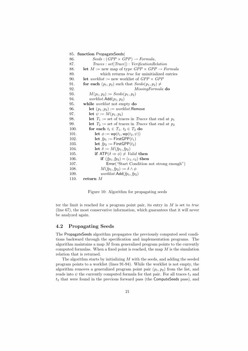
time timeDescription P T I (PO) (no PO)

min:sec min:sec1. Simple buffer 7 7 29 00:00 00:002. Simple vending machine 2 2 20 00:00 00:003. Cyclic scheduler 11 6 65 00:49 01:014. Student tracking system 11 3 63 00:01 00:015. 1 comm link 13 11 54 00:01 00:016. 2 parallel comm links 22 18 105 00:04 01:287. 3 parallel comm links 27 25 144 00:21 514:528. 4 parallel comm links 32 32 186 01:11 DNT9. 5 parallel comm links 37 39 228 02:32 DNT10. 6 parallel comm links 42 46 270 08:29 DNT11. 7 parallel comm links 47 53 312 37:28 DNT12. SystemC refinement 8 8 39 00:00 00:0013. EP2 system 7 3 173 01:47 01:51

Table 1: Refinement examples checked using our tool (P stands for “Numberof Process Description”, T stands for “Number of parallel Threads”, I standsfor “Number of Instructions”, PO stands for “partial order reduction”, DNTstands for “did not terminate”)

that end at p1 and p2, the algorithm computes the weakest precondition of ψwith respect to the two traces (lines 98-101). The algorithm then appropriatelystrengthens the formula stored at the beginning of the two traces using thecomputed weakest precondition (lines 102-108). In particular, if the formula δstored at the beginning of the two traces does not imply the newly computedweakest precondition, then the weakest precondition is added as a conjunct toδ.

The approach of deriving seeds in a forward pass, and then propagating theseeds in a backward pass using weakest preconditions was inspired by Necula’stranslation validation work [30] for checking the equivalence of two sequentialprograms. The intuition behind why such a simple approach works well inpractice is that the control flow of the specification and the implementation areoften similar, and the relation required to show equivalence are usually simple,involving only linear equalities of variables.

5 Evaluation

To evaluate our algorithm we implemented it using the Simplify theoremprover [12] in a verification system called ARCCoS. We then wrote a variety ofCSP refinements, and checked them for correctness automatically. The refine-ments that we checked are shown in Table 1, along with the number of processesfor each example, the number of parallel threads, the number of instructions,

22

the time required to check each example using partial order reduction (PO),and the time required without partial order reduction (no PO). The first 11refinements were inspired from examples that come with the FDR tool [2]. The6th example in this list, named “2 parallel comm links” is the example presentedin Section 2.2. We also implemented generalizations of these 11 FDR examplesto make them data-dependent and operate over infinite domains. We were ableto check these generalized refinements that FDR would not be able to check.

The 12th refinement in the list is a hardware refinement example takenfrom a SystemC book [16]. This example models the refinement of an abstractFIFO communication channel to an implementation that uses a standard FIFOhardware channel, along with logic to make the hardware channel correctlyimplement the abstract communication channel.

In the 13th refinement from Table 1, we checked part of the EP2 system [1],which is a new industrial standard for electronic payments. We followed theimplementation of the data part of the EP2 system found in a recent TACAS 05paper on CSP-Prover [19]. The EP2 system states how various components,including service centers, credit card holders, and terminals, interact.

In all of the above examples, since trace subset refinement preserves safetyproperties, we can conclude that the implementation has all the safety propertiesof the specification.

We also have a large test suite of incorrect refinements that we run our toolon, to make sure that our tool indeed detects these as incorrect refinements.

Aside from providing refinement guarantees, our tool was also useful in find-ing subtle bugs in our original implementation of some refinements. For exam-ple, in the refinement presented in Section 2.2, we originally did not implementan acknowledgment link, which made the refinement incorrect. In this samerefinement, we also mistakenly used parallel composition || instead of externalchoice � in msg sender. Our tool found these mistakes, and we were able torectify them.

6 Related Work

As mentioned in the introduction, there has been a long line of work on reason-ing about refinement of CSP programs. Our relational checking algorithm wasinspired by Josephs’s approach [20] for proving refinements. However, Josephsproved refinements by hand, whereas our tool is fully automated. Our searchingalgorithm through the control state of the program is similar to FDR’s searchingtechnique [2], which exhaustively explores the state space. However, as men-tioned previously, our tool can handle infinite state spaces that do not triviallyreduce using skolemization to finite state spaces.

Various interactive theorem provers have been extended with the ability toreason about CSP programs. As one example, Dutertre and Schneider [13] rea-soned about communication protocols expressed as CSP programs using thePVS theorem prover [31]. As another example, Tej and Wolff [39] have usedthe Isabelle theorem prover [32] to encode the semantics of CSP programs. Is-

23

abelle has also been used by Isobe and Roggenbach to develop a tool calledCSP-Prover [19] for proving properties of CSP programs. All these uses ofinteractive theorem provers follow a common high-level approach: the seman-tics of CSP is usually encoded using the native logic of the interactive theoremprover, and then a set of tactics are defined for reasoning about this semantics.Users of the system can then write proof scripts that use these tactics, along withbuilt-in tactics from the theorem prover, to prove properties about particularCSP programs. Our approach does not have the same level of formal underpin-nings as these interactive theorem proving approaches. However, our approachis fully automated, whereas these interactive theorem proving approaches allrequire some amount of human intervention.

Our inference algorithm was inspired by Necula’s translation validationwork [30], and bears similarities with Necula’s algorithm for inferring simula-tion relations that prove equivalence of sequential programs. Necula’s algorithmcollects a set of constraints in a forward scan of the two programs, and thensolves these constraints using a specialized solver and expression simplifier. Un-like Necula’s approach, our algorithm is expressed in terms of calls to a generaltheorem prover, rather than using specialized solvers and simplifiers. Our algo-rithm is also more modular, in the sense that the theorem proving part of thealgorithm has been modularized into a component with a very simple interface(it takes a formula and returns Valid or Invalid).

7 Conclusion and future work

We have presented an automated algorithm for checking trace refinement ofconcurrent systems modeled as CSP programs. The proposed refinement check-ing algorithm is implemented in a validation system called ARCCoS and wedemonstrated its effectiveness through a variety of examples.

We have expanded the class of CSP programs that FDR can handle withvariables that include unbounded integers. FDR cannot handle these programssince it requires variables to have fixed bit widths. Even though some of ourexamples were taken from FDR’s test suite, these examples were changed byconverting the data type of the variables to unbounded integers. Once we dothat, these programs cannot be handled by FDR. In this sense, our contributionis to incorporate an automated theorem proving capability to FDR’s searchtechnique in order to handle infinite state spaces that are data-dependent.

Our work solves the critical problem of handling more sophisticated data-types than finite bit-width enumeration types associated with typical RTL codeand thus enables stepwise refinement of system designs expressed using high-level languages. Our ongoing effort is on building a validation system thatautomatically checks SystemC refinements through translation validation fortheir use in synthesis environments.

24

References

[1] EP2. www.eftpos2000.ch.

[2] Failures-divergence refinement: FDR2 user manual. Formal Systems (Eu-rope) Ltd., Oxford, England, June 2005.

[3] R. Allen and D. Garlan. A formal basis for architectural connection. ACMTransactions on Software Engineering and Methodology, 6(3):213–249, July1997.

[4] T. Ball, R. Majumdar, T. Millstein, and S. K. Rajamani. Automatic pred-icate abstraction of C programs. In Proceedings PLDI 2001, June 2001.

[5] Nick Benton. Simple relational correctness proofs for static analyses andprogram transformations. In POPL 2004, January 2004.

[6] A. Benveniste, L. Carloni, P. Caspi, and A. Sangiovanni-Vincentelli. Het-erogeneous reactive systems modeling and correct-by-construction deploy-ment, 2003.

[7] J. R. Burch, E. M. Clarke, K. L. McMillan, D. L. Dill, and L. J. Hwang.Symbolic model checking: 1020 states and beyond. In Proceedings of LICS1990, 1990.

[8] Doran Bustan and Orna Grumberg. Simulation based minimization. InDavid A. McAllester, editor, CADE 2000, volume 1831 of LNCS, pages255–270. Springer Verlag, 2000.

[9] S. Chaki, E. Clarke, J. Ouaknine, N. Sharygina, and N. Sinha. Concurrentsoftware verification with states, events and deadlocks. Formal Aspects ofComputing Journal, 17(4):461–483, December 2005.

[10] E. M. Clarke and David E. Long Orna Grumberg. Verification tools forfinite-state concurrent systems. In A Decade of Concurrency, Reflectionsand Perspectives, volume 803 of LNCS. Springer Verlag, 1994.

[11] C.N. Ip and D.L. Dill. Better verification through symmetry. In D. Agnew,L. Claesen, and R. Camposano, editors, Computer Hardware DescriptionLanguages and their Applications, pages 87–100, Ottawa, Canada, 1993.Elsevier Science Publishers B.V., Amsterdam, Netherland.

[12] D. Detlefs, G. Nelson, and J. B. Saxe. Simplify: A theorem prover forprogram checking. Journal of the Association for Computing Machinery,52(3):365–473, May 2005.

[13] B. Dutertre and S. Schneider. Using a PVS embedding of CSP to ver-ify authentication protocols. In TPHOL 97, Lecture Notes in ArtificialIntelligence. Springer-Verlag, 1997.

25

[14] C. Flanagan, K. R. M. Leino, M. Lillibridge, G. Nelson, J. B. Saxe, andR. Stata. Extended static checking for Java. In PLDI 2002, June 2002.

[15] Susanne Graf and Hassen Saidi. Construction of abstract state graphs ofinfinite systems with PVS. In CAV 97, June 1997.

[16] T. Grotker. System Design with SystemC. Kluwer Academic Publishers,2002.

[17] Thomas A. Henzinger, Ranjit Jhala, Rupak Majumdar, and Gregoire Sutre.Lazy abstraction. In POPL 2002, January 2002.

[18] C. A. R. Hoare. Communicating Sequential Processes. Prentice Hall Inter-national, 1985.

[19] Yoshinao Isobe and Markus Roggenbach. A generic theorem prover of CSPrefinement. In TACAS ’05, volume 1503 of Lecture Notes in ComputerScience (LNCS), pages 103–123. Springer-Verlag, April 2005.

[20] Mark B. Josephs. A state-based approach to communicating processes.Distributed Computing, 3(1):9–18, March 1988.

[21] Moshe Y. Vardi Kathi Fisler. Bisimulation and model checking. In Proceed-ings of the 10th Conference on Correct Hardware Design and VerificationMethods, Bad Herrenalb Germany CA, September 1999.

[22] David Lacey, Neil D. Jones, Eric Van Wyk, and Carl Christian Frederiksen.Proving correctness of compiler optimizations by temporal logic. In POPL2002, January 2002.

[23] Edward A. Lee and Alberto L. Sangiovanni-Vincentelli. A framework forcomparing models of computation. IEEE Trans. on CAD of IntegratedCircuits and Systems, 17(12):1217–1229, 1998.

[24] Stan Liao, Steve Tjiang, and Rajesh Gupta. An efficient implementationof reactivity for modeling hardware in the scenic design environment. InDAC ’97: Proceedings of the 34th annual conference on Design automation,pages 70–75, New York, NY, USA, 1997. ACM Press.

[25] Panagiotis Manolios, Kedar S. Namjoshi, and Robert Summers. Linkingtheorem proving and model-checking with well-founded bisimulation. InCAV ’99: Proceedings of the 11th International Conference on ComputerAided Verification, pages 369–379, London, UK, 1999. Springer-Verlag.

[26] Panagiotis Manolios and Sudarshan K. Srinivasan. Automatic verificationof safety and liveness for xscale-like processor models using web refinements.In DATE ’04: Proceedings of the conference on Design, automation andtest in Europe, page 10168, Washington, DC, USA, 2004. IEEE ComputerSociety.

26

[27] K. L. McMillan. A compositional rule for hardware design. In CAV 97,1997.

[28] K. L. McMillan. Verification of an implementation of tomasulos algorithmby compositional model checking. In CAV 98, 1998.

[29] K. L. McMillan. A methodology for hardware verification using composi-tional model checking. Sci. Comput. Program., 37(1-3):279–309, 2000.

[30] George C. Necula. Translation validation for an optimizing compiler. InPLDI 2000, June 2000.

[31] S. Owre, J.M. Rushby, and N. Shankar. PVS: A prototype verificationsystem. In CADE 92. Springer-Verlag, 1992.

[32] L. C. Paulson. Isabelle: A generic theorem prover, volume 828 of LecureNotes in Computer Science. Springer Verlag, 1994.

[33] D. Peled. Ten years of partial order reduction. In CAV 98, June 1998.

[34] A. Pnueli, M. Siegel, and E. Singerman. Translation validation. In TACAS’98, volume 1384 of Lecture Notes in Computer Science, pages 151–166,1998.

[35] A. Roscoe. The Theory and Practice of Concurrency. Prentice Hall, 1998.

[36] A. W. Roscoe, P. H. B. Gardiner, M. H. Goldsmith, J. R. Hulance, D. M.Jackson, and J. B. Scattergood. Hierarchical compression for model-checking CSP or how to check 1020 dining philosophers for deadlock. InTACAS ’95, 1995.

[37] Ingo Sander and Axel Jantsch. System modeling and transformationaldesign refinement in forsyde [formal system design]. IEEE Trans. on CADof Integrated Circuits and Systems, 23(1):17–32, 2004.

[38] J. P. Talpin, P. L. Guernic, S. K. Shukla, F. Doucet, and R. Gupta. Formalrefinement checking in a system-level design methodology. FundamentaInformaticae, 62(2):243–273, 2004.

[39] H. Tej and B.Wolff. A corrected failure-divergence model for CSP in Is-abelle/HOL. In FME 97, 1997.

27