Spacetime Meshing with Adaptive Refinement and Coarsening∗

Reza Abedi† Shuo-Heng Chung‡ Jeff Erickson‡§ Yong Fan† Michael Garland‡

Damrong Guoy¶ Robert Haber† John M. Sullivan‖ Shripad Thite‡ Yuan Zhou‡

Center for Process Simulation and Design

University of Illinois at Urbana-Champaign

rabedi,schung6,jeffe,yongfan,garland,guoy,r-haber,jms,thite,yuanzhou@uiuc.edu

ABSTRACT

We propose a new algorithm for constructing finite-elementmeshes suitable for spacetime discontinuous Galerkin solu-tions of linear hyperbolic PDEs. Given a triangular meshof some planar domain Ω and a target time value T , ourmethod constructs a tetrahedral mesh of the spacetime do-main Ω × [0, T ] in constant running time per tetrahedronin IR3 using an advancing front method. Elements are addedto the evolving mesh in small patches by moving a vertex ofthe front forward in time. Spacetime discontinuous Galerkinmethods allow the numerical solution within each patch tobe computed as soon as the patch is created. Our algo-rithm employs new mechanisms for adaptively coarseningand refining the front in response to a posteriori error esti-mates returned by the numerical code. A change in the frontinduces a corresponding refinement or coarsening of futureelements in the spacetime mesh. Our algorithm adapts theduration of each element to the local quality, feature size,and degree of refinement of the underlying space mesh. Wedirectly exploit the ability of discontinuous Galerkin meth-ods to accommodate discontinuities in the solution fieldsacross element boundaries.

∗See http://www.cs.uiuc.edu/∼jeffe/pubs/refine.html for themost recent version of this paper. Work on this paper was par-tially supported by NSF ITR grant DMR-0121695.†Department of Theoretical and Applied Mechanics, Universityof Illinois at Urbana-Champaign, Urbana, IL 61801 (UIUC).‡Department of Computer Science, UIUC.§Also partially supported by NSF CAREER award CCR-0093348and NSF ITR grant CCR-0219594.¶Center for Simulation of Advanced Rockets (CSAR), Compu-tational Science and Engineering Program, UIUC. The CSARresearch program is supported by the US Department of Energythrough the University of California under subcontract B523819.‖Department of Mathematics, UIUC, and Department of Math-ematics, Technische Universitat Berlin. Also partially supportedby NSF grant DMS-00-71520.

Permission to make digital or hard copies of all or part of this work forpersonal or classroom use is granted without fee provided that copies arenot made or distributed for profit or commercial advantage and that copiesbear this notice and the full citation on the first page. To copy otherwise, torepublish, to post on servers or to redistribute to lists, requires prior specificpermission and/or a fee.SCG’04, June 8–11, 2004, Brooklyn, New York, USA.Copyright 2004 ACM 1-58113-885-7/04/0006 ...$5.00.

Categories and Subject Descriptors: I.3.5 [ComputerGraphics]: Computational geometry and object modeling—Geometric algorithms, languages, and systems; F.2.2 [Anal-ysis of Algorithms and Problem Complexity]: Nonnumeri-cal algorithms and problems—Geometric problems and com-

putations; G.1.8 [Numerical Analysis]: Partial differentialequations—Hyperbolic equations; finite element methods

Keywords: mesh generation, unstructured meshes, tetra-hedral meshes, spacetime discontinuous Galerkin, advancingfront, adaptivity

General Terms: Algorithms, Performance

1. INTRODUCTION

Scientists and engineers use conservation laws and hyper-bolic partial differential equations to model transient, wave-like behavior in bodies or spatial control volumes. Exampleapplications are numerous, ranging from the Euler equationsfor compressible gas dynamics, to the Schrodinger equationfor time-dependent density functional theory in quantummechanics, to the equations of elastodynamics in seismicanalysis. Closed-form solutions are typically unavailable forthese problems, so analysts usually resort to numerical ap-proximations. However, the continuum solutions can exhibitstrongly nonlinear behavior as well as shocks and other dis-continuities that make this class of numerical problems par-ticularly challenging.

Finite element methods are a good option for solving theseproblems, especially when the geometry of the analysis do-main is complicated. In the standard semi-discrete approach,a finite element mesh discretizes space to generate a systemof ordinary differential equations in time that is then solvedby a time-marching integration scheme. Most methods en-force a uniform time step size over the entire spatial domain.This approach can be very costly for strongly graded grids,because the allowable time step size is limited by the globalminimum element diameter. However, physical causalityonly implies a local limit on the step size, so algorithms thatuse a nonuniform time step size can substantially improvecomputational efficiency.

Dynamic adaptive refinement and coarsening is essentialfor capturing solution features that move with traveling in-terfaces and shock fronts. Each discrete remeshing opera-tion requires a projection of the solution fields from the oldgrid onto the newly adapted mesh. These projections canbe costly and inconvenient to compute, and they introduce

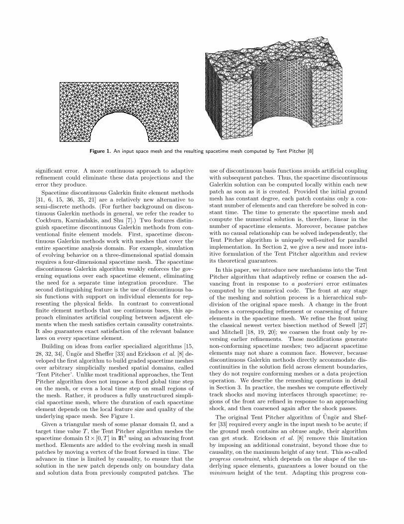
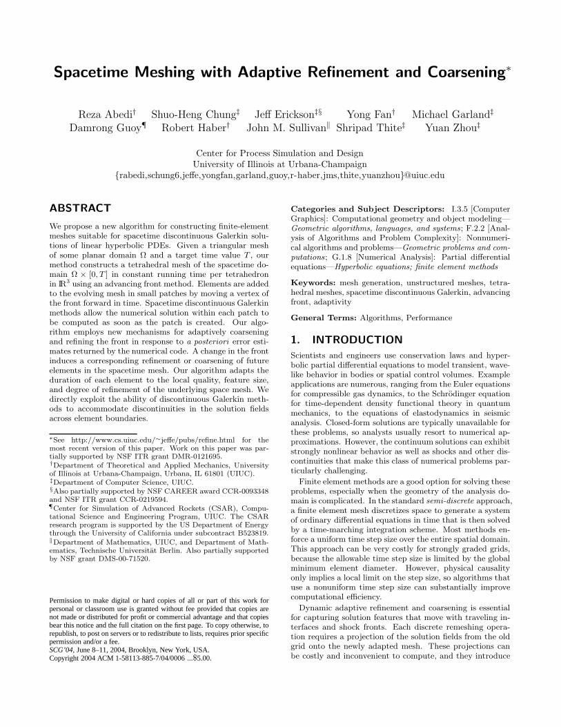
Figure 1. An input space mesh and the resulting spacetime mesh computed by Tent Pitcher [8]

significant error. A more continuous approach to adaptiverefinement could eliminate these data projections and theerror they produce.

Spacetime discontinuous Galerkin finite element methods[31, 6, 15, 36, 35, 21] are a relatively new alternative tosemi-discrete methods. (For further background on discon-tinuous Galerkin methods in general, we refer the reader toCockburn, Karniadakis, and Shu [7].) Two features distin-guish spacetime discontinuous Galerkin methods from con-ventional finite element models. First, spacetime discon-tinuous Galerkin methods work with meshes that cover theentire spacetime analysis domain. For example, simulationof evolving behavior on a three-dimensional spatial domainrequires a four-dimensional spacetime mesh. The spacetimediscontinuous Galerkin algorithm weakly enforces the gov-erning equations over each spacetime element, eliminatingthe need for a separate time integration procedure. Thesecond distinguishing feature is the use of discontinuous ba-sis functions with support on individual elements for rep-resenting the physical fields. In contrast to conventionalfinite element methods that use continuous bases, this ap-proach eliminates artificial coupling between adjacent ele-ments when the mesh satisfies certain causality constraints.It also guarantees exact satisfaction of the relevant balancelaws on every spacetime element.

Building on ideas from earlier specialized algorithms [15,

28, 32, 34], Ungor and Sheffer [33] and Erickson et al. [8] de-veloped the first algorithm to build graded spacetime meshesover arbitrary simplicially meshed spatial domains, called‘Tent Pitcher’. Unlike most traditional approaches, the TentPitcher algorithm does not impose a fixed global time stepon the mesh, or even a local time step on small regions ofthe mesh. Rather, it produces a fully unstructured simpli-cial spacetime mesh, where the duration of each spacetimeelement depends on the local feature size and quality of theunderlying space mesh. See Figure 1.

Given a triangular mesh of some planar domain Ω, and atarget time value T , the Tent Pitcher algorithm meshes thespacetime domain Ω× [0, T ] in IR3 using an advancing frontmethod. Elements are added to the evolving mesh in smallpatches by moving a vertex of the front forward in time. Theadvance in time is limited by causality, to ensure that thesolution in the new patch depends only on boundary dataand solution data from previously computed patches. The

use of discontinuous basis functions avoids artificial couplingwith subsequent patches. Thus, the spacetime discontinuousGalerkin solution can be computed locally within each newpatch as soon as it is created. Provided the initial groundmesh has constant degree, each patch contains only a con-stant number of elements and can therefore be solved in con-stant time. The time to generate the spacetime mesh andcompute the numerical solution is, therefore, linear in thenumber of spacetime elements. Moreover, because patcheswith no causal relationship can be solved independently, theTent Pitcher algorithm is uniquely well-suited for parallelimplementation. In Section 2, we give a new and more intu-itive formulation of the Tent Pitcher algorithm and reviewits theoretical guarantees.

In this paper, we introduce new mechanisms into the TentPitcher algorithm that adaptively refine or coarsen the ad-vancing front in response to a posteriori error estimatescomputed by the numerical code. The front at any stageof the meshing and solution process is a hierarchical sub-division of the original space mesh. A change in the frontinduces a corresponding refinement or coarsening of futureelements in the spacetime mesh. We refine the front usingthe classical newest vertex bisection method of Sewell [27]and Mitchell [18, 19, 20]; we coarsen the front only by re-versing earlier refinements. These modifications generatenon-conforming spacetime meshes; two adjacent spacetimeelements may not share a common face. However, becausediscontinuous Galerkin methods directly accommodate dis-continuities in the solution field across element boundaries,they do not require conforming meshes or a data projectionoperation. We describe the remeshing operations in detailin Section 3. In practice, the meshes we compute effectivelytrack shocks and moving interfaces through spacetime; re-gions of the front are refined in response to an approachingshock, and then coarsened again after the shock passes.

The original Tent Pitcher algorithm of Ungor and Shef-fer [33] required every angle in the input mesh to be acute; ifthe ground mesh contains an obtuse angle, their algorithmcan get stuck. Erickson et al. [8] remove this limitationby imposing an additional constraint, beyond those due tocausality, on the maximum height of any tent. This so-calledprogress constraint, which depends on the shape of the un-derlying space elements, guarantees a lower bound on theminimum height of the tent. Adapting this progress con-

straint to support the changing geometry of the front is themain technical contribution of this paper; see Section 4.

In Section 5 we describe a 2D×time linear elastodynam-ics simulation computed with the help of our meshing al-gorithm. Finally, we conclude the paper by describing ourongoing work and open problems in spacetime meshing.

2. SPACETIME MESHING

The formulation of our spacetime meshing problem relies onthe notions of domain of influence and domain of depen-dence for hyperbolic boundary value problems. We say thata point p in spacetime depends on another point q if thevalues of the salient physical fields (e.g., temperature, ve-locity, pressure, stress, momentum) at p depend on the fieldvalues at q; that is, if changing the conditions at q can affectthe conditions at p. The domain of influence of p is the setof points that depend on p; symmetrically, the domain of

dependence is the set of points that p depends on.

If the governing equations of the underlying problem arelinear and the material properties are homogeneous andisotropic, the domains of influence and dependence are cir-cular cones with a common apex p. This double cone canbe described by a scalar wave speed c(p) ∈ IR, which speci-fies how quickly the radius of the cones grows as a functionof time. In this paper, we consider only linear problems,where the wave speed is uniform and isotropic over the en-tire spacetime domain. In this case, we can choose an ap-propriate time scale, independent of the spatial scale, sothat c(p) = 1 everywhere. For more general problems, thewave speed can vary with direction and as a function of in-homogeneous physical parameters, and might even dependnonlinearly on the solution.

We say that one spacetime element 4 depends on anotherspacetime element 4′ if any point p ∈ 4 depends on anypoint q ∈ 4′. The solution can be computed in each elementone at a time, following any linear extension of the depen-dency partial order. Alternatively, the solutions within anyanti-chain of elements can be computed in parallel.

Although discontinuous Galerkin methods impose no a

priori restrictions on the primitive shapes of individual el-ements, it is convenient to work with simplicial elements.We say that a facet F of a tetrahedral element is causal if itseparates the cone of influence from the cone of dependenceat every point on F (Figure 2), or equivalently, if ‖∇F‖ ≤ 1.If a facet is causal, physical information flows in only onedirection across that facet. To construct an efficient tetra-hedral mesh, we group elements into patches, each with aconstant number of elements. The Tent Pitcher algorithmensures that the boundary facets between patches are causal

by construction; we refer to this requirement as the causality

constraint (called the cone constraint in Erickson et al. [8]).

In general, the internal facets between elements within asingle patch are not causal. Since information can flow inboth directions across these facets, the physical response inadjacent elements is coupled, and all of the elements withina patch must therefore be solved simultaneously. However,if we assume polynomial basis functions of bounded degree,the resulting linear system still has bounded size and cantherefore be solved in constant time. Thus, the total time tocompute the numerical solution is still linear in the numberof elements.

tim

e

Figure 2. The causality constraint: The facet separates the cone ofinfluence (above) from the cone of dependence (below).

Richter [22] observed that undesirable numerical dissipa-tion increases in certain discontinuous Galerkin methods asthe slopes of boundary facets decrease below the local wavespeed. Thus, our goal is to construct an efficient mesh com-prised of patches, each containing a small number of sim-plices, such that the boundary facets of each patch are asclose as possible to the cone constraint without violating it.

2.1 Advancing-Front Spacetime Meshing

Given a triangulated planar domain Ω and a target timevalue T , Tent Pitcher constructs a tetrahedral mesh of thespacetime domain Ω × [0, T ]. The algorithm is designed asan advancing front procedure, which alternately constructsa new patch of elements and invokes a spacetime discontinu-ous Galerkin finite-element method to compute the solutionwithin that patch.

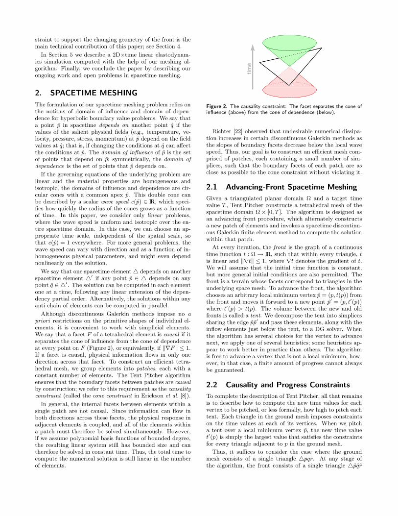
At every iteration, the front is the graph of a continuoustime function t : Ω → IR, such that within every triangle, tis linear and ‖∇t‖ ≤ 1, where ∇t denotes the gradient of t.We will assume that the initial time function is constant,but more general initial conditions are also permitted. Thefront is a terrain whose facets correspond to triangles in theunderlying space mesh. To advance the front, the algorithmchooses an arbitrary local minimum vertex p = (p, t(p)) fromthe front and moves it forward to a new point p′ = (p, t′(p))where t′(p) > t(p). The volume between the new and oldfronts is called a tent. We decompose the tent into simplicessharing the edge pp′ and pass these elements, along with theinflow elements just below the tent, to a DG solver. Whenthe algorithm has several choices for the vertex to advancenext, we apply one of several heuristics; some heuristics ap-pear to work better in practice than others. The algorithmis free to advance a vertex that is not a local minimum; how-ever, in that case, a finite amount of progress cannot alwaysbe guaranteed.

2.2 Causality and Progress Constraints

To complete the description of Tent Pitcher, all that remainsis to describe how to compute the new time values for eachvertex to be pitched, or less formally, how high to pitch eachtent. Each triangle in the ground mesh imposes constraintson the time values at each of its vertices. When we pitcha tent over a local minimum vertex p, the new time valuet′(p) is simply the largest value that satisfies the constraintsfor every triangle adjacent to p in the ground mesh.

Thus, it suffices to consider the case where the groundmesh consists of a single triangle 4pqr. At any stage ofthe algorithm, the front consists of a single triangle 4pqr

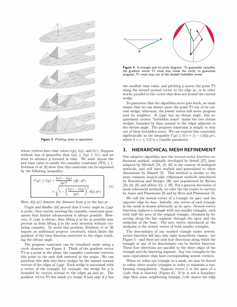
Figure 3. Pitching tents in spacetime.

whose vertices have time values t(p), t(q), and t(r). Supposewithout loss of generality that t(p) ≤ t(q) ≤ t(r) and wewant to advance p forward in time. We must choose thenew time value to satisfy the causality constraint ‖∇t‖ ≤ 1.Erickson et al. [8] show that this constraint can be expressedby the following inequality:

t′(p) ≤ t(q) +t(r) − t(q)

|qr|2( ~qp · ~qr)

+

s

1 −

„

t(r) − t(q)

|qr|

«2

d(p, qr)

(1)

Here, d(p, qr) denotes the distance from p to the line qr.

Ungor and Sheffer [33] proved that if every angle in 4pqris acute, then exactly meeting the causality constraint guar-antees that further advancement is always possible. How-ever, if ∠pqr is obtuse, then lifting p as far as possible mayprevent us from lifting q in the next iteration without vio-lating causality. To avoid this problem, Erickson et al. [8]impose an additional progress constraint, which limits thegradient of the time function restricted to the edges touch-ing the obtuse angle.

The progress constraint can be visualized easily using acircle diagram; see Figure 4. Think of the gradient vector∇t as a point in the plane; the causality constraint restrictsthis point to the unit disk centered at the origin. We canpartition this disk into three wedges by the inward normalvectors of the edges of 4pqr. Each wedge is associated witha vertex of the triangle; for example, the wedge for p isbounded by vectors normal to the edges pq and pr. Thegradient vector ∇t lies inside p’s wedge if and only if p has

p

qr

Figure 4. A triangle and its circle diagram. To guarantee causality,the gradient vector ∇t must stay inside the circle; to guaranteeprogress, ∇t must stay out of the shaded forbidden zones.

the smallest time value, and pitching p moves the point ∇talong the inward normal vector to the edge qr, or in otherwords, parallel to the vector that does not bound the currentwedge.

To guarantee that the algorithm never gets stuck, we mustensure that we can always move the point ∇t out of its cur-rent wedge; otherwise, the lowest vertex will never progresspast its neighbor. If 4pqr has an obtuse angle, this re-quirement creates “forbidden zones” inside the two obtusewedges, bounded by lines normal to the edges adjacent tothe obtuse angle. The progress constraint is simply to stayout of these forbidden zones. We can express this constraintalgebraically as the inequality t′(p) ≤ t(r) + (1 − ε)d(p, qr),where 0 < ε ≤ 1/2 is a tunable parameter.

3. HIERARCHICAL MESH REFINEMENT

Our adaptive algorithm uses the newest-vertex bisection re-finement method, originally developed by Sewell [27], lateradapted by Mitchell [18, 19, 20] in the context of multigridmethods, and still later studied and generalized to threedimensions by Bansch [3]. This method is similar to themore common longest-edge refinement methods introducedby Rosenberg and Stenger [26] and popularized by Rivara[23, 24, 25] and others [12, 1, 29]. For a general discussion ofmesh refinement methods, we refer the the reader to surveysby Jones and Plassmann [9] and by Bern and Plassmann [4].

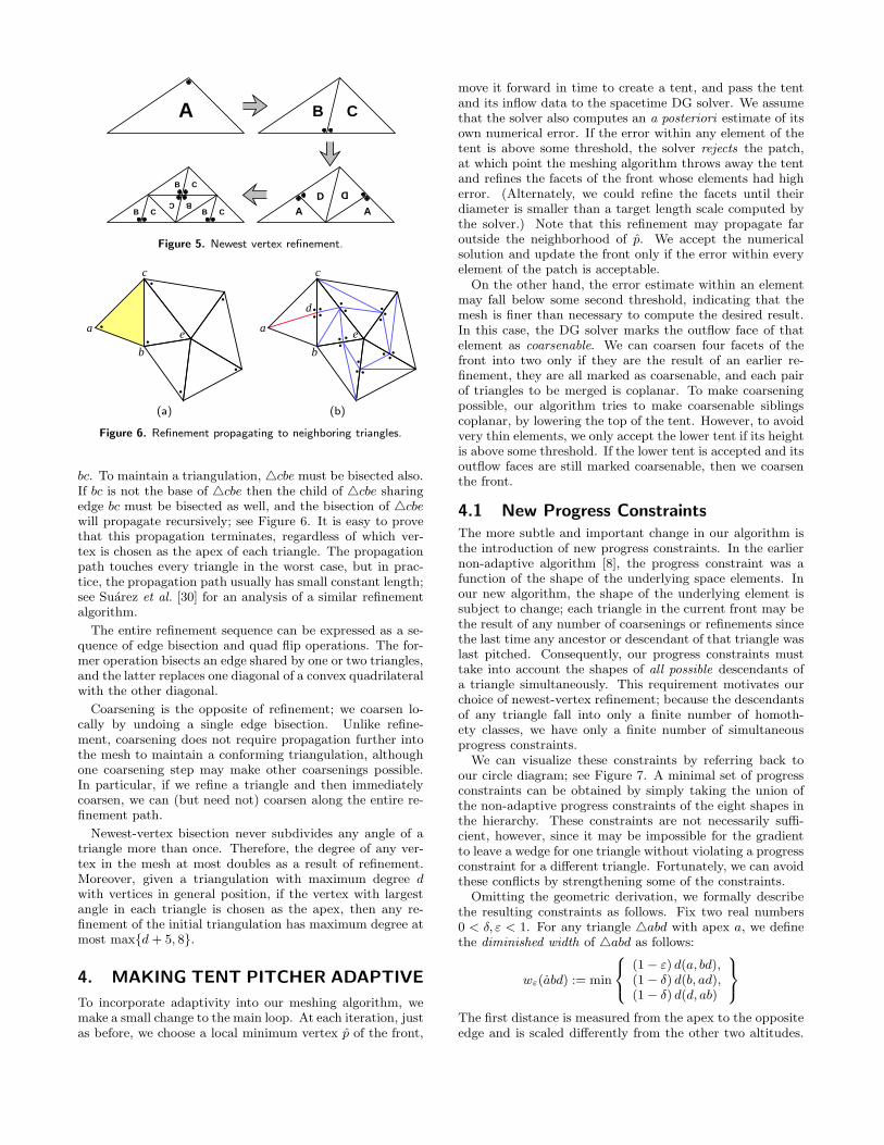
We call the newest vertex of a triangle its apex and theopposite edge its base. Initially, one vertex of each trianglein the mesh is chosen arbitrarily as its apex. Newest-vertexbisection replaces a triangle with two smaller triangles, eachwith half the area of the original triangle, obtained by bi-secting along the line segment through the apex and themidpoint of the base. The new vertex introduced at themidpoint is the newest vertex of both smaller triangles.

The descendants of any marked triangle under newest-vertex bisection fall into only eight homothetic classes—seeFigure 5—and there are only four directions along which thetriangle or any of its descendants can be further bisected.These four directions are parallel to the three edges of thetriangle and the bisecting segment. Any two triangles in thesame equivalence class have corresponding newest vertices.

When we refine one triangle in a mesh, we may be forcedto refine other nearby triangles in order to maintain a con-forming triangulation. Suppose vertex a is the apex of a4abc that is bisected (Figure 6). If bc is not a boundaryedge then some neighboring triangle 4cbe shares the edge

A B C

A AD

D

B C B C

B C

BC

Figure 5. Newest vertex refinement.

a

b

c

e

d

a

b

c

e

(a) (b)

Figure 6. Refinement propagating to neighboring triangles.

bc. To maintain a triangulation, 4cbe must be bisected also.If bc is not the base of 4cbe then the child of 4cbe sharingedge bc must be bisected as well, and the bisection of 4cbewill propagate recursively; see Figure 6. It is easy to provethat this propagation terminates, regardless of which ver-tex is chosen as the apex of each triangle. The propagationpath touches every triangle in the worst case, but in prac-tice, the propagation path usually has small constant length;see Suarez et al. [30] for an analysis of a similar refinementalgorithm.

The entire refinement sequence can be expressed as a se-quence of edge bisection and quad flip operations. The for-mer operation bisects an edge shared by one or two triangles,and the latter replaces one diagonal of a convex quadrilateralwith the other diagonal.

Coarsening is the opposite of refinement; we coarsen lo-cally by undoing a single edge bisection. Unlike refine-ment, coarsening does not require propagation further intothe mesh to maintain a conforming triangulation, althoughone coarsening step may make other coarsenings possible.In particular, if we refine a triangle and then immediatelycoarsen, we can (but need not) coarsen along the entire re-finement path.

Newest-vertex bisection never subdivides any angle of atriangle more than once. Therefore, the degree of any ver-tex in the mesh at most doubles as a result of refinement.Moreover, given a triangulation with maximum degree dwith vertices in general position, if the vertex with largestangle in each triangle is chosen as the apex, then any re-finement of the initial triangulation has maximum degree atmost maxd + 5, 8.

4. MAKING TENT PITCHER ADAPTIVE

To incorporate adaptivity into our meshing algorithm, wemake a small change to the main loop. At each iteration, justas before, we choose a local minimum vertex p of the front,

move it forward in time to create a tent, and pass the tentand its inflow data to the spacetime DG solver. We assumethat the solver also computes an a posteriori estimate of itsown numerical error. If the error within any element of thetent is above some threshold, the solver rejects the patch,at which point the meshing algorithm throws away the tentand refines the facets of the front whose elements had higherror. (Alternately, we could refine the facets until theirdiameter is smaller than a target length scale computed bythe solver.) Note that this refinement may propagate faroutside the neighborhood of p. We accept the numericalsolution and update the front only if the error within everyelement of the patch is acceptable.

On the other hand, the error estimate within an elementmay fall below some second threshold, indicating that themesh is finer than necessary to compute the desired result.In this case, the DG solver marks the outflow face of thatelement as coarsenable. We can coarsen four facets of thefront into two only if they are the result of an earlier re-finement, they are all marked as coarsenable, and each pairof triangles to be merged is coplanar. To make coarseningpossible, our algorithm tries to make coarsenable siblingscoplanar, by lowering the top of the tent. However, to avoidvery thin elements, we only accept the lower tent if its heightis above some threshold. If the lower tent is accepted and itsoutflow faces are still marked coarsenable, then we coarsenthe front.

4.1 New Progress Constraints

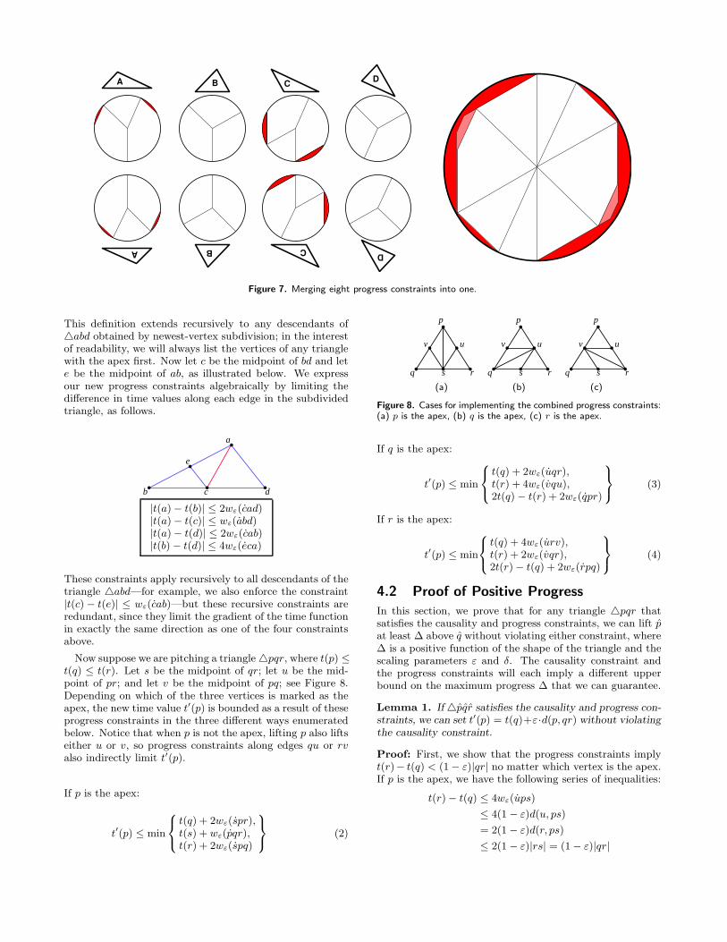
The more subtle and important change in our algorithm isthe introduction of new progress constraints. In the earliernon-adaptive algorithm [8], the progress constraint was afunction of the shape of the underlying space elements. Inour new algorithm, the shape of the underlying element issubject to change; each triangle in the current front may bethe result of any number of coarsenings or refinements sincethe last time any ancestor or descendant of that triangle waslast pitched. Consequently, our progress constraints musttake into account the shapes of all possible descendants ofa triangle simultaneously. This requirement motivates ourchoice of newest-vertex refinement; because the descendantsof any triangle fall into only a finite number of homoth-ety classes, we have only a finite number of simultaneousprogress constraints.

We can visualize these constraints by referring back toour circle diagram; see Figure 7. A minimal set of progressconstraints can be obtained by simply taking the union ofthe non-adaptive progress constraints of the eight shapes inthe hierarchy. These constraints are not necessarily suffi-cient, however, since it may be impossible for the gradientto leave a wedge for one triangle without violating a progressconstraint for a different triangle. Fortunately, we can avoidthese conflicts by strengthening some of the constraints.

Omitting the geometric derivation, we formally describethe resulting constraints as follows. Fix two real numbers0 < δ, ε < 1. For any triangle 4abd with apex a, we definethe diminished width of 4abd as follows:

wε(abd) := min

8

<

:

(1 − ε) d(a, bd),(1 − δ) d(b, ad),(1 − δ) d(d, ab)

9

=

;

The first distance is measured from the apex to the oppositeedge and is scaled differently from the other two altitudes.

B

B

D

D

A

A

C

C

Figure 7. Merging eight progress constraints into one.

This definition extends recursively to any descendants of4abd obtained by newest-vertex subdivision; in the interestof readability, we will always list the vertices of any trianglewith the apex first. Now let c be the midpoint of bd and lete be the midpoint of ab, as illustrated below. We expressour new progress constraints algebraically by limiting thedifference in time values along each edge in the subdividedtriangle, as follows.

a

b c d

e

|t(a) − t(b)| ≤ 2wε(cad)|t(a) − t(c)| ≤ wε(abd)|t(a) − t(d)| ≤ 2wε(cab)|t(b) − t(d)| ≤ 4wε(eca)

These constraints apply recursively to all descendants of thetriangle 4abd—for example, we also enforce the constraint|t(c) − t(e)| ≤ wε(cab)—but these recursive constraints areredundant, since they limit the gradient of the time functionin exactly the same direction as one of the four constraintsabove.

Now suppose we are pitching a triangle 4pqr, where t(p) ≤t(q) ≤ t(r). Let s be the midpoint of qr; let u be the mid-point of pr; and let v be the midpoint of pq; see Figure 8.Depending on which of the three vertices is marked as theapex, the new time value t′(p) is bounded as a result of theseprogress constraints in the three different ways enumeratedbelow. Notice that when p is not the apex, lifting p also liftseither u or v, so progress constraints along edges qu or rvalso indirectly limit t′(p).

If p is the apex:

t′(p) ≤ min

8

<

:

t(q) + 2wε(spr),t(s) + wε(pqr),t(r) + 2wε(spq)

9

=

;

(2)

q

u

p

r

v

s q

u

p

r

v

s q

u

p

r

v

s

(a) (b) (c)

Figure 8. Cases for implementing the combined progress constraints:(a) p is the apex, (b) q is the apex, (c) r is the apex.

If q is the apex:

t′(p) ≤ min

8

<

:

t(q) + 2wε(uqr),t(r) + 4wε(vqu),2t(q) − t(r) + 2wε(qpr)

9

=

;

(3)

If r is the apex:

t′(p) ≤ min

8

<

:

t(q) + 4wε(urv),t(r) + 2wε(vqr),2t(r) − t(q) + 2wε(rpq)

9

=

;

(4)

4.2 Proof of Positive Progress

In this section, we prove that for any triangle 4pqr thatsatisfies the causality and progress constraints, we can lift pat least ∆ above q without violating either constraint, where∆ is a positive function of the shape of the triangle and thescaling parameters ε and δ. The causality constraint andthe progress constraints will each imply a different upperbound on the maximum progress ∆ that we can guarantee.

Lemma 1. If 4pqr satisfies the causality and progress con-

straints, we can set t′(p) = t(q)+ε·d(p, qr) without violating

the causality constraint.

Proof: First, we show that the progress constraints implyt(r)− t(q) < (1 − ε)|qr| no matter which vertex is the apex.If p is the apex, we have the following series of inequalities:

t(r) − t(q) ≤ 4wε(ups)

≤ 4(1 − ε)d(u, ps)

= 2(1 − ε)d(r, ps)

≤ 2(1 − ε)|rs| = (1 − ε)|qr|

Here, the first inequality is the actual progress constraint,the second follows from the definition of diminished width,and the rest follow from the geometry of the recursivelybisected triangle. Similarly, if q is the apex, we have

t(r) − t(q) ≤ 2wε(upq)

≤ 2(1 − ε)d(u, pq)

= (1 − ε)d(r, pq) ≤ (1 − ε)|qr|,

and if r is the apex, we have

t(r) − t(q) ≤ 2wε(vpr)

≤ 2(1 − ε)d(v, pr)

= (1 − ε)d(q, pr) ≤ (1 − ε)|qr|.

Solving for ε gives us the inequality

ε ≤ 1 −t(r) − t(q)

|qr|≤

s

1 −

„

t(r) − t(q)

|qr|

«2

,

which implies that

t′(p) = t(q) + ε · d(p, qr)

≤ t(q) +

s

1 −

„

t(r) − t(q)

|qr|

«2

d(p, qr)

≤ t(q) +t(r) − t(q)

|qr|2( ~qp · ~qr)

+

s

1 −

„

t(r) − t(q)

|qr|

«2

d(p, qr).

This is exactly the expression of the causality constraint inequation (1).

Lemma 2. If 0 < ε < δ < (1 + ε)/2 < 1 and 4pqrsatisfies the causality and progress constraints, we can set

t′(p) = t(q) + ∆ without violating any progress constraint,

where ∆ > 0 is a function of the triangle 4pqr and the

parameters ε and δ.

Proof: As in the previous proof, we have three cases toconsider. In each case, we will derive positive upper boundson the possible value of ∆; setting ∆ to the minimum ofthese upper bounds will satisfy the conditions of the lemma.

First, suppose p is marked. Since t(r) ≥ t(s) ≥ t(q), therelevant progress constraint (2) is satisfied if

∆ ≤ min2wε(spr), wε(pqr), 2wε(spq).

Similarly, suppose r is marked. Since t(r) ≥ t(q), we have2t(r) − 2t(q) ≥ 0, which implies that the relevant progressconstraint (4) is satisfied if

∆ ≤ min4wε(urv), 2wε(vqr), 2wε(rpq).

Finally, suppose q is marked. By the inductive hypothesis,edge qr already satisfies its individual progress constraintt(r) ≤ t(q) + 2wε(upq), which implies that t(q) − t(r) ≥−2wε(upq). Since t(r) ≥ t(q), the relevant progress con-straint (3) is satisfied if

∆ ≤ min2wε(uqr), 4wε(vqu), 2wε(qpr) − 2wε(upq).

The last term in this expression is the only one that is notobviously positive. To prove that X = wε(qpr) − wε(upq)

is in fact bounded away from zero, we expand the definitionof diminished width. We have X = minA, B, C, where

A = (1 − ε)d(q, pr) − min

8

<

:

(1 − ε)d(u, pq),(1 − δ)d(p, qu),(1 − δ)d(q, pu)

9

=

;

≥ (1 − ε)d(q, pr) − (1 − δ)d(q, pu)

= (δ − ε)d(q, pr),

B = (1 − δ)d(r, pq) − min

8

<

:

(1 − ε)d(u, pq),(1 − δ)d(p, qu),(1 − δ)d(q, pu)

9

=

;

≥ (1 − δ)d(r, pq) − (1 − ε)d(u, pq)

= (1 − 2δ + ε)d(u, pq),

C = (1 − δ)d(p, qr) − min

8

<

:

(1 − ε)d(u, pq),(1 − δ)d(p, qu),(1 − δ)d(q, pu)

9

=

;

≥ (1 − δ)`

d(p, qr) − min d(p, qu), d(q, pu)´

.

Since by assumption ε < δ < (1 + ε)/2, we clearly haveA > 0 and B > 0. We prove that C > 0 as follows:

d(p, qr) =2Area(4pqr)

|qr|

=2Area(4pqu)

|uv|

>2Area(4pqu)

max |qu|, |pu|

= min d(p, qu), d(q, pu) .

The key observation is that the bisector segment uv mustbe shorter than at least one of the two edges pu and qu.

Theorem 3. Given a triangular mesh Ω in the plane and a

target time value T , our algorithm builds a finite tetrahedral

mesh of the spacetime domain Ω×[0, T ], in constant running

time per element, provided each triangle is refined only a

finite number of times.

5. EXPERIMENTAL RESULTS

We have implemented our adaptive spacetime meshing al-gorithm in 1D×time and 2D×time. We present here an ex-ample to demonstrate its application to a scientific problemof practical complexity: the phenomenon of crack-tip wavescattering within an elastic solid subjected to shock loading.

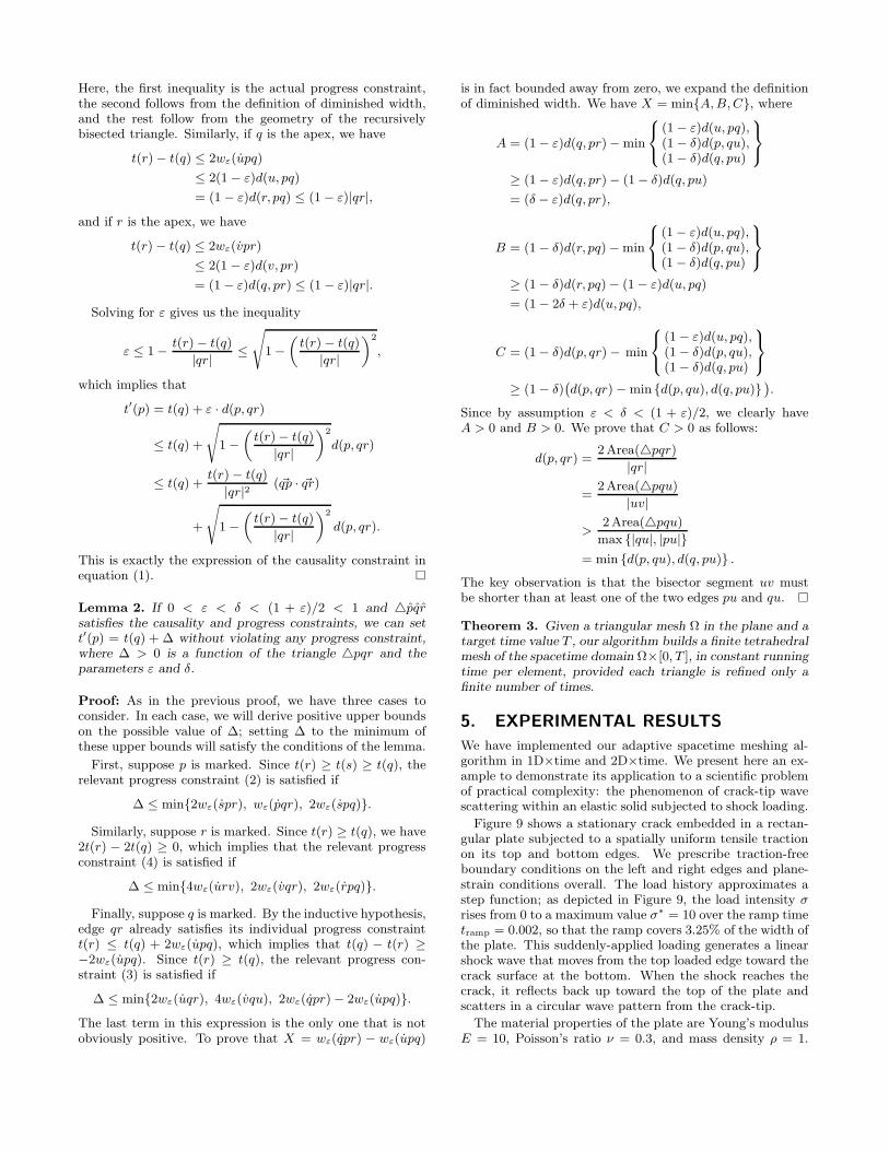
Figure 9 shows a stationary crack embedded in a rectan-gular plate subjected to a spatially uniform tensile tractionon its top and bottom edges. We prescribe traction-freeboundary conditions on the left and right edges and plane-strain conditions overall. The load history approximates astep function; as depicted in Figure 9, the load intensity σrises from 0 to a maximum value σ∗ = 10 over the ramp timetramp = 0.002, so that the ramp covers 3.25% of the width ofthe plate. This suddenly-applied loading generates a linearshock wave that moves from the top loaded edge toward thecrack surface at the bottom. When the shock reaches thecrack, it reflects back up toward the top of the plate andscatters in a circular wave pattern from the crack-tip.

The material properties of the plate are Young’s modulusE = 10, Poisson’s ratio ν = 0.3, and mass density ρ = 1.

σ

σ time

σLoad

tramp

(a) (b)

Figure 9. Crack geometry and loading for the crack-tip wave scat-tering problem.

Since the domain and initial conditions are symmetric, weexplicitly model only the upper right quadrant of the do-main, specifying symmetric boundary conditions at the leftand bottom edges. The initial space mesh contains only 16triangles; we depend on the adaptive meshing algorithm togenerate all of the necessary refinement. We use a com-plete quadratic polynomial basis (1 x y t xy yt tx x2 y2 t2)to represent the displacement field within each tetrahedralspacetime element.

A dissipation-based error indicator drives the adaptivemeshing scheme. The energy dissipated by each patch iscompared to the total energy flux into the patch; zero dissi-pation indicates exact energy balance. We set a normalizeddissipation target, dissipation/energy influx = 1.0 × 10−7.Elements with dissipation more than 20% above the targetare rejected and marked for mandatory refinement. Ele-ments with dissipation more than 20% below the target areaccepted and marked as eligible for coarsening. We alsospecify a minimum dissipation of 6.0 × 10−10 and a mini-mum element size of 5.0 × 10−5, below either of which nofurther refinement is allowed.

The final spacetime mesh contains 17, 052, 587 tetrahe-dra, clustered into 2, 964, 477 patches. During the solutionprocess, 3, 679, 040 patches containing 21, 956, 046 tetrahe-dra were computed and solved; approximately 20% of thesepatches were rejected, causing the front to be refined. Theratio of the largest to smallest element diameters in thespacetime mesh is 1024, reflecting 20 levels of refinement.The normalized dissipation for the entire spacetime analysisdomain is 0.079%.

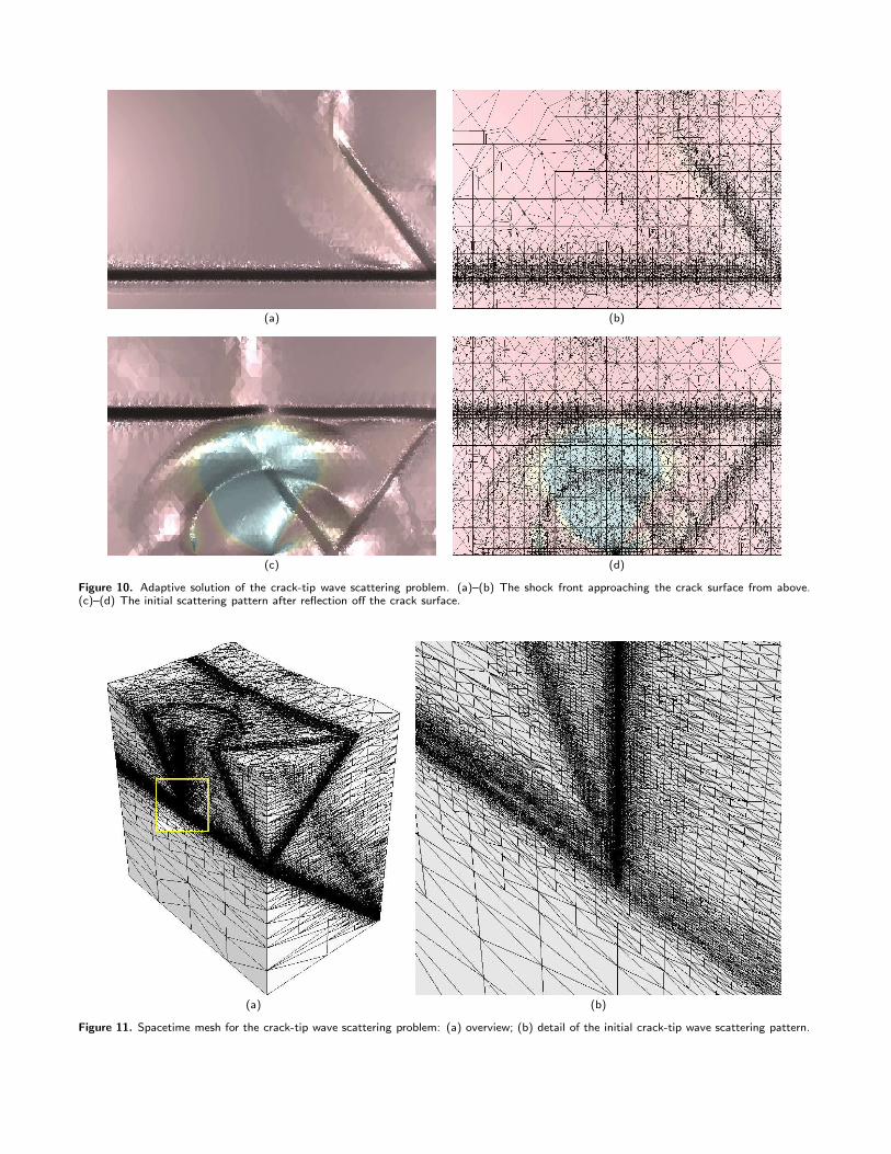
Figure 10 shows two pairs of visualizations of the com-puted solution within the upper right quadrant of the plate.Each image illustrates the intersection of the spacetime dataset with a constant-time plane. The images on the leftdisplay two axes of the solution data, by mapping strain-energy-density to a color field on a logarithmic scale, andmapping the magnitude of the velocity field to a height field.The images on the right show the intersection of the unstruc-tured tetrahedral spacetime mesh with the constant-timeplane, together with the strain-energy-density color field.

The first pair of images in Figure 10 show the shock frontas it approaches the crack surface for the first time. Thepattern of mesh refinement accurately tracks the fine detailsof the traveling waves, including the primary shock frontas well as dilitation and shear waves generated along thetraction-free top edge.

The second pair of images show the initial crack-tip wavescattering pattern some time after the shock first arrives atthe crack. The circular scattering pattern is reflected in themesh refinement; the outer annulus of less intense refinementindicates the extent of the faster dilitational wave compo-nent, while the circle of more intense refinement indicatesthe slower shear wave. A singular strain-energy-density fieldis visible at the crack tip, a stationary feature that generatesa persistent region of intense mesh refinement.

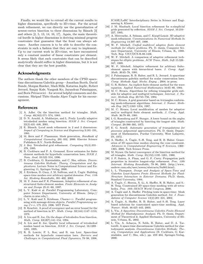
Figure 11 shows two views of the entire spacetime meshat roughly the same time depicted in the second row of Fig-ures 10. The vertical axis is time, and the pattern of re-finement on the vertical faces follows closely the spacetimetrajectories of the shocks; see Figure 11(a). The cone-shapedregion of intense mesh refinement in Figure 11(b) covers thedomain of influence of the initial crack-tip scattering event.The asymmetry of the cone is consistent with the form ofthe singular crack-tip field, which vanishes in the plane ofthe crack ahead (to to the right) of the tip.

As expected, our experimental results show a significantimprovement in the quality of the solution as a result ofadaptivity, especially near discontinuities in the solution orits derivative. Also, we were able to achieve a better solutionwithout using a fine mesh everywhere, which would haveresulted in a massive increase in computation time.

6. CURRENT AND FUTURE WORK

We implemented a sequential version of our adaptive TentPitcher algorithm for one- and two-dimensional spatial do-mains which we used to solve linear PDEs with constantwavespeed and nonlinear problems where the maximum wave-speed is bounded. We also prototyped a parallel versionfor 1D×time that leverages the mutual independence of anytwo patches over the same front. Since the patches can besolved independently of each other, we were able to solvethem simultaneously on different processors. We used theCHARM++ parallel language and runtime system [11] de-veloped by the Parallel Programming Group at the Univer-sity of Illinois [10] to manage interprocessor communication,load balancing, and the automatic dispatch and schedulingof patches to be solved. In our preliminary experiments, weobserved a parallel speedup of about 20. We observed thatthe speedup was limited mainly by the mesh generation,which was not running in parallel.

We are also investigating spacetime discontinuous Galerkinmethods for nonlinear conservation laws. In such problems,the wavespeed is not constant throughout the spacetime do-main. Instead, the wavespeed is one of the physical pa-rameters governed by the underlying PDE, and can there-fore change in unpredictable ways. We have extended TentPitcher to adapt the number and duration of spacetime el-ements to changing wavespeeds, for problems defined overone- and two-dimensional spatial domains. As in the cur-rent paper, the major theoretical bottleneck lies in develop-ing appropriate progress constraints. We have implementedour algorithm for nonlinear problems in 1D×time, and weare currently implementing the algorithm in 2D×time. Weexpect to publish these results in a subsequent paper.

We are also working on combining the mesh refinementwith adaptivity to local wavespeeds. We plan to implementthis combined, completely adaptive algorithm in parallel.

(a) (b)

(c) (d)

Figure 10. Adaptive solution of the crack-tip wave scattering problem. (a)–(b) The shock front approaching the crack surface from above.(c)–(d) The initial scattering pattern after reflection off the crack surface.

(a) (b)

Figure 11. Spacetime mesh for the crack-tip wave scattering problem: (a) overview; (b) detail of the initial crack-tip wave scattering pattern.

Finally, we would like to extend all the current results tohigher dimensions, specifically to 3D×time. For the actualmesh refinement, we can directly use the generalization ofnewest-vertex bisection to three dimensions by Bansch [3]and others [2, 5, 13, 14, 16, 17]. Again, the main theoreti-cal hurdle in higher dimensions is deriving minimal progressconstraints that guarantee that the front can always ad-vance. Another concern is to be able to describe the con-straints in such a fashion that they are easy to implement.Up to our current work in 2D×time, we have encounteredonly a constant number of linear constraints per element.It seems likely that such constraints that can be describedanalytically should suffice in higher dimensions, but it is notclear that they are the best possible.

Acknowledgments

The authors thank the other members of the CPSD space-time discontinuous Galerkin group—Jonathan Booth, DavidBunde, Morgan Hawker, Mark Hills, Katarina Jegdic, RobertJerrard, Sanjay Kale, Yangsuk Ko, Jayandran Palaniappan,and Boris Petracovici—for several helpful comments and dis-cussions. Shripad Thite thanks Alper Ungor for his encour-agement.

References[1] A. Adler. On the bisection method for triangles. Math.

Comp. 40(162):571–574, 1983.[2] D. N. Arnold, A. Mukherjee, and L. Pouly. Locally adaptive

tetrahedral meshes using bisection. SIAM J. Sci. Comput.22(2):431–448, 2001.

[3] E. Bansch. Local mesh refinement in 2 and 3 dimensions.Impact of Computing in Science and Engineering 3:181–191,1991.

[4] M. Bern and P. Plassmann. Mesh generation. Handbook ofComputational Geometry, 291–332, 2000. Elsevier SciencePublishers B.V. North-Holland.

[5] J. Bey. Tetrahedral grid refinement. Computing 55(4):355–378, 1995.

[6] B. Cockburn and P. A. Gremaud. Error estimates for finiteelement methods for hyperbolic conservation laws. SIAM J.Num. Anal. 33:522–554, 1996.

[7] B. Cockburn, G. Karniadakis, and C. Shu, editors. Discon-tinuous Galerkin Methods: Theory, Computation and Ap-plications. Lecture Notes in Computational Science and En-gineering 11, Springer-Verlag, 2000.

[8] J. Erickson, D. Guoy, J. M. Sullivan, and A. Ungor. Buildingspace-time meshes over arbitrary spatial domains. Proc. 11thInt. Meshing Roundtable, 391–402, 2002.

[9] M. T. Jones and P. E. Plassmann. Adaptive refinement of un-structured finite-element meshes. Finite Elements in Analy-sis and Design 25:41–60, 1997.

[10] L. V. Kale et al. Parallel Programming Laboratory, Com-puter Science Department, University of Illinois. 〈http://charm.cs.uiuc.edu/〉.

[11] L. V. Kale and S. Krishnan. Charm++: Parallel program-ming with message-driven objects. Parallel Programming us-ing C++, 175–213, 1996. MIT Press.

[12] B. Kearfott. A proof of covergence and an error bound for themethod of bisection in R

n. Math. Comp. 32(144):1147–1153,1978.

[13] A. Liu and B. Joe. On the shape of tetrahedra from bisection.Math. Comp. 63(207):141–154, 1994.

[14] A. Liu and B. Joe. Quality local refinement of tetrahedralmeshes based on bisection. SIAM J. Sci. Comput. 16:1269–1291, 1995.

[15] R. B. Lowrie, P. L. Roe, and B. van Leer. Space-timemethods for hyperbolic conservation laws. Barriers andChallenges in Computational Fluid Dynamics, 79–98, 1998.

ICASE/LaRC Interdisciplinary Series in Science and Engi-neering 6, Kluwer.

[16] J. M. Maubach. Local bisection refinement for n-simplicialgrids generated by reflection. SIAM J. Sci. Comput. 16:210–227, 1995.

[17] A. Merrouche, A. Selman, and C. Knopf-Lenoir. 3D adaptivemesh refinement. Communications In Numerical Methods InEngineering 14:397–407, 1998.

[18] W. F. Mitchell. Unified multilevel adaptive finite elementmethods for elliptic problems. Ph. D. thesis, Computer Sci-ence Department, University of Illinois, Urbana, IL, 1988.Tech. Rep. UIUCDCS-R-88-1436.

[19] W. F. Mitchell. A comparison of adaptive refinement tech-niques for elliptic problems. ACM Trans. Math. Soft 15:326–347, 1989.

[20] W. F. Mitchell. Adaptive refinement for arbitrary finite-element spaces with hierarchical bases. J. Comp. Appl.Math. 36:65–78, 1991.

[21] J. Palaniappan, R. B. Haber, and R. L. Jerrard. A spacetimediscontinuous galerkin method for scalar conservation laws.Comp. Methods Appl. Mechs. Engng. , 2004. in press.

[22] G. R. Richter. An explicit finite element method for the waveequation. Applied Numerical Mathematics 16:65–80, 1994.

[23] M. C. Rivara. Algorithms for refining triangular grids suit-able for adaptive and multigrid techniques. Internat. J. Nu-mer. Methods Eng. 20:745–756, 1984.

[24] M. C. Rivara. A grid generator based on 4-triangles conform-ing mesh-refinement algorithms. Internat. J. Numer. Meth-ods Eng. 24(7):1343–1354, 1987.

[25] M. C. Rivara. Local modification of meshes for adaptiveand/or multigrid finite element methods. J. Comp. Appl.Math. 36:79–89, 1991.

[26] I. G. Rosenberg and F. Stenger. A lower bound on the anglesof triangles constructed by bisecting the longest side. Math.Comput. 29:390–395, 1975.

[27] E. G. Sewell. Automatic generation of triangulations forpiecewise polynomial approximation. Ph. D. thesis, Depart-ment of Mathematics, Purdue University, West Lafayette,IN, 1972.

[28] A. Sheffer, A. Ungor, S.-H. Teng, and R. B. Haber. Gener-ation of 2D space-time meshes obeying the cone constraint.Advances in Computational Engineering & Sciences, 1360–1365, 2000. Tech Science Press.

[29] M. Stynes. On faster convergence of the bisection method forall triangles. Math. Comp. 35(152):1195–1201, 1980.

[30] J. P. Suarez, A. Plaza, and G. F. Carey. Propagation pathproperties in iterative longest-edge refinement. Proc. 12thInternat. Meshing Roundtable, 79–90, 2003. 〈http://www.andrew.cmu.edu/user/sowen/abstracts/Su983.html〉.

[31] L. L. Thompson. Design and Analysis of Space-Time andGalerkin Least-Squares Finite Element Methods for Fluid-Structure Interaction in Exterior Domains. Ph.D. thesis,Stanford University, 1994.

[32] A. Ungor, C. Heeren, X. Li, A. Sheffer, R. B. Haber, and S.-H. Teng. Constrained 2D space-time meshing with all tetra-hedra. Proc. 16th IMACS World Congress, 2000.

[33] A. Ungor and A. Sheffer. Pitching tents in space-time: Meshgeneration for discontinuous Galerkin method. Int. J. Foun-dations of Computer Science 13(2):201–221, 2002.

[34] A. Ungor, A. Sheffer, R. B. Haber, and S.-H. Teng. Layerbased solutions for constrained space-time meshing. Appl.Numer. Math. 46:425–443, 2003.

[35] L. Yin. A Spacetime Discontinuous Galerkin Finite-ElementMethod for Elastodynamic Analysis. Ph. D. thesis, Depart-ment of Theoretical & Applied Mechanics, University of Illi-nois, Urbana, IL, 2002.

[36] L. Yin, A. Acharya, N. Sobh, R. Haber, and D. A. Tor-torelli. A space-time discontinuous Galerkin method for elas-todynamic analysis. Discontinuous Galerkin Methods: The-ory, Computation and Applications (B. Cockburn, G. Kar-niadakis, and C. Shu, eds.), pp. 459–464. Springer-Verlag,2000.