18th World IMACS / MODSIM Congress, Cairns, Australia 13-17 July 2009 http://mssanz.org.au/modsim09

River bathymetry from conventional LiDAR using water surface returns

Smart, G.M.1, J. Bind 1 and M.J. Duncan1

1 National Inst. of Water & Atmospheric Research, Box 8602, Christchurch, New Zealand. Email: g.smart@niwa.co.nz

Abstract: LiDAR–based DEMs are almost essential when it comes to high resolution floodplain modelling. Conventional LiDAR does not penetrate water bodies and additional bathymetric measurements are necessary to complete any parts of a DEM which were under water at the time of the LiDAR sortie. Bathymetric data collection is time-consuming, expensive and it requires careful processing to correctly interpolate between sounded points or cross-sections and to seamlessly integrate bathymetric data into a LiDAR-based DEM. Consequently, accuracy of underwater portions of a DEM is usually inferior to that of dry areas. When areas that are underwater at LiDAR collection time represent only a small portion of a flood domain, modelers often estimate a representative depth for these areas.

By using LiDAR returns from the surface of flowing water, we investigate calculations to predict the level of the underlying river bed using a hydraulic model. To do this, there must be sufficient LiDAR returns from the water surface, the river flow must be known at the time of the LiDAR data collection and information on the roughness of the river bed is required. An assumed bed topography is used with the hydraulic model to predict the water surface elevation. The error between predicted water surface elevation and LiDAR-measured water surface elevation is then used iteratively to adjust the assumed bed position until the correct water surface elevation is calculated.

The technique was applied to a 1024 by 512 meter reach of the gravel-bed Waiau River on the Canterbury Plains on the eastern side of the South Island of New Zealand. The river flow was 17.96 m3/s during the LiDAR data collection and about an 80 m width of the channel fairway was underwater. Comprehensive bathymetry measurements made with an echo sounder and RTK GPS were used to evaluate the model-predicted bed levels.

The iterative hydraulic model technique predicted the bed level with high accuracy in locations where the Froude number was > 0.3. For these conditions 41% of the predicted bed levels lay within ± 10 cm and 85% of the predicted levels lay within ± 30 cm of the GPS-measured bed level.

The Froude number influence may reflect the fact that the technique can not work if there is no water movement. The technique should not be applied to ponds, lakes or very slow flowing water.

Further tests are required to cover a wider range of river conditions.

Keywords: LiDAR, inverse hydraulic modelling, bathymetry, inundation, water-surface returns.

2521

Smart et Bind., River bathymetry from conventional LiDAR using water surface returns

1. INTRODUCTION

Two-dimensional (depth averaged) hydraulic models are becoming commonplace for river flood inundation modelling. With such models, overland flow paths, local water depths, velocities, bed scour, bank erosion, sediment transport, and hazard indices can be calculated. These models solve the Shallow-Water Equations (SWE, e.g. Abbott, 1979) for each node of a grid or mesh covering a river’s channels and floodplains. Each node must be assigned a topographic elevation and roughness. This requires high resolution terrain information.

Airborne LiDAR can provide topographic information with a high degree of automation, a high point density (more than one point per m2) and elevation accuracy of better than ±15 cm. Unfortunately, conventional red-laser LiDAR does not penetrate water bodies and bathymetric measurements are necessary to complete any parts of a DEM (Digital Elevation Model) which were under water at the time of the LiDAR data collection. For water up to around 1 meter deep the bathymetric data can be collected by wading with a GPS. For deeper water it is necessary to use a boat with an on-board GPS and depth sounder. In some situations, particularly turbulent or fast flowing rivers, it is not possible to use either method and modelers must estimate the channel depth with other techniques. Where underwater locations (at LiDAR collection time) represent a small portion of a flood’s domain, modelers may chose to adopt a constant, representative depth for these areas. In all such cases the data requires careful processing to interpolate between sounded points, cross-sections or estimates and to seamlessly integrate the bathymetric data into the LiDAR-based DEM.

In many cases the missing underwater DEM locations will have LiDAR returns from the water’s surface. These are useful if a representative depth can be estimated or calculated for a water body. A constant “cross-section average” water depth can be estimated using the channel flow, slope and roughness and a flow resistance equation such as the Manning Equation (e.g. Henderson, 1966). The average depth is subtracted from the local water surface elevation to give the local bed elevation. In essence this is an inverse application of hydraulic modeling to predict the position of the bed, in comparison with the usual application where the position of the bed is used to predict the location of the water surface.

The sensitivity of cross-sectional geometry parameters to inverse hydraulic modelling was investigated with a simple 1-dimensional model by Roux and Dartus (2008) who carried out ten thousand Monte Carlo simulation runs for a trapezoidal channel with sloping flood berms. They concluded that, for their sub-critical flow conditions, the water level at the downstream boundary was the most important parameter and the influence of other factors such as the flow resistance coefficient or bed slope were very small in comparison. Flow criticality is indicated by the Froude number Fr which compares inertial and gravitational forces. Flow is sub-critical when Fr < 1.0 and when this occurs, the flow at a given location is influenced by conditions downstream of that location.

2. MODEL FOR CALCULATING BED LEVEL FROM KNOWN WATER SURFACE LEVEL

An alternative to an analytical approach to investigate unique inverse solution of the shallow water equations, is to calculate the local level of a river bed by iteration. An assumed bed topography can be used in a conventional SWE solving hydraulic model to predict the water surface elevation. The error between predicted water surface elevation and known water surface elevation would then (repeatedly) be used to adjust the assumed bed level until the correct water surface elevation was calculated. To achieve such an iterative solution, information on the roughness of the river bed is required, there must be sufficient LiDAR returns from the water surface to represent changes in the water surface level, the river flow must be known at the time of the LiDAR data collection and the iteration technique must converge.

3. ITERATION CONVERGENCE TECHNIQUE

An algorithm is required to correct errors in the bed elevation y, given a known error in the water surface elevation, w. According to the Manning Eq. velocity in a steady, depth-averaged flow can be calculated as:

v = C(w-y) 2/3 (1)

where C = (S1/2/n), S is the energy gradient and n the Manning roughness coefficient (Henderson, 1966).

Re-arranging (1) gives:

y = w ± (v/C)3/2 (2)

Substituting the equation of continuity v = q/(w-y), where q is discharge per unit width, in (2) gives:

y = w ± (q/C)3/5 (3)

2522

Smart et Bind., River bathymetry from conventional LiDAR using water surface returns

While channel slope and roughness depend on elevation on a catchment scale, for local hydraulics, the factor C is assumed independent of y or w. As the discharge is constant along a channel section, an approximate assumption can also be made that the discharge per unit width q is independent of bed elevation or water surface elevation.

On this basis, differentiating (3) gives dy/dw = 1 i.e. Δy = Δw (4)

Thus, as an initial approximation, a small error in the water surface Δw is caused by an equivalent error in the bed level Δy.

4. TEST APPLICATION

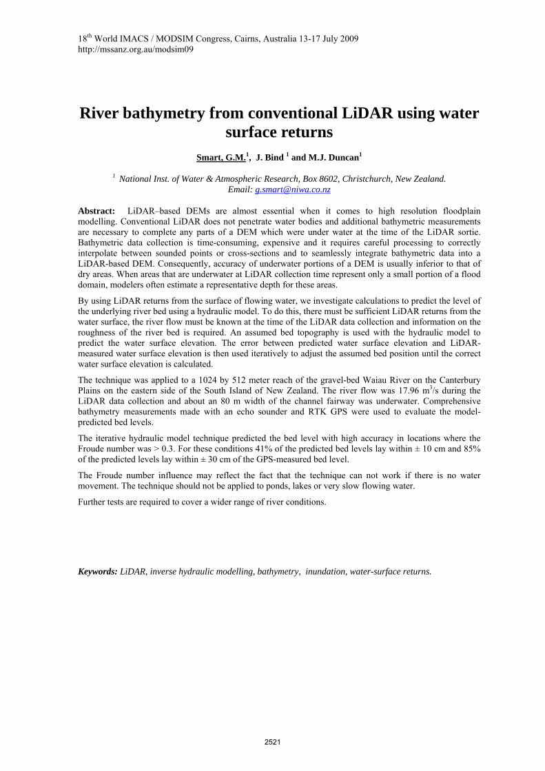
A 1024 by 512 meter reach of the gravel bed Waiau River on the Canterbury Plains on the eastern side of the South Island of New Zealand was used to evaluate the proposed iterative technique. The site was selected because comprehensive LiDAR data, RTK GPS ground survey information and bed material analyses were available. The average slope of the river channel was 0.4%. The channel had a flow of 17.96 m3/s during the LiDAR data collection and about 80 m width of the fairway was underwater. An aerial photo of the site is shown in Figure 1.

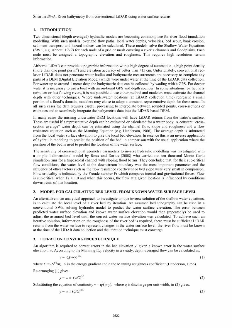
Geospatial information used for the model evaluation is shown in Figure 2. These are LiDAR returns from the water surface (shown in white) and bathymetry measurements made with RTK GPS (red, green and blue). The average spacing of the GPS soundings was 0.12 spot heights per m2 and the LiDAR water surface hits were spaced at 1.42 hits per m2 on average.

5. COMPUTATION GRIDS FROM GEOSPATIAL INFORMATION

5.1. Water surface LiDAR DEM

The irregularly spaced LiDAR water surface hits were converted to a TIN and this was linearly interpolated to give a DEM representing water surface elevations at grid nodes on a 1024 x 512 grid of one meter squares.

5.2. River bed DEM from GPS survey points and LiDAR

The irregularly spaced GPS point measurements were converted to a TIN and linearly interpolated to give a DEM representing GPS-measured river bed elevations at grid nodes (the centre of grid squares) on the same 1024 x 512 grid. When bathymetric measurements are available this is a standard method for creating an underwater DEM for use in a hydraulic model.

5.3. River bed DEM from LIDAR water hits

The position of the river channel bed was approximated by assuming a fixed river channel depth of 0.4 m below the position of the water surface LiDAR DEM. The 0.4 m depth was estimated from on-site observations at the time of the LiDAR measurements. Such a DEM has very steep underwater banks but may be suitable for flood modelling purposes where much of the flow passes over the more accurately mapped floodplains.

Figure 2. Model domain with locations for GPS bed levels (red, green and blue) and LiDAR surface returns (white). The black arrow and outline show the area covered by perspective views in Figure 5.

Figure 1. Site location for testing the iterative bed model. Area shown is approx. 1 km x 0.7 km. River flow is from left to right.

2523

Smart et Bind., River bathymetry from conventional LiDAR using water surface returns

6. APPLICATION OF THE ITERATIVE MODEL

The level of the river channel bed was initially approximated by assuming a fixed channel depth of 0.4 m below the water surface LiDAR DEM as described above. A depth-averaged 2 dimensional hydraulic model Hydro2de (Beffa and Connell, 2001) was used to predict the water surface elevation for an inflow of 17.96 m3/s (the flow at the time of the LiDAR sortie), channel roughness Zo = 0.01 m and the uniform depth downstream conditions for a channel slope of 0.4%. The model predicted water surface elevations that were, on average, 9 cm too low with a standard deviation in the Δw errors of 15 cm. In places Δw errors were large, especially where there was little water movement. To reduce propagation of these errors a correction was applied based on model-calculated bed shear stress σb. If σb was greater than 2 N/m2 (an arbitrary threshold indicating motion) the bed elevation was corrected by 90% of the water surface prediction error. If σb was less than 2 N/m2 the correction coefficient was reduced from 90% to zero as the local σb reduced from 2 N/m2 to 0. A further constraint was applied to ensure that the correction could not result in a water depth that was less than 5 cm (because if the channel became dry there would be no water level).

The model bed elevation grid nodes were corrected according to these rules and the hydraulic model was re-run to calculate new water surface elevations. The predicted water surface elevations were now, on average, 18 cm too high with an error standard deviation of 8.3 cm. The process was repeated until the 5th iteration by which time the water surface elevations were 1.9 cm too high with an error standard deviation of 5.3 cm. These errors were used to correct the bed level as before and the resulting topography is discussed below. Considering that airborne LiDAR measured levels can have an error standard deviation of 15 cm, the errors in predicted water levels were considered to be very satisfactory.

7. VERIFICATION OF THE RESULTS

7.1. Comparison of LiDAR/GPS based DEM with GPS measurements

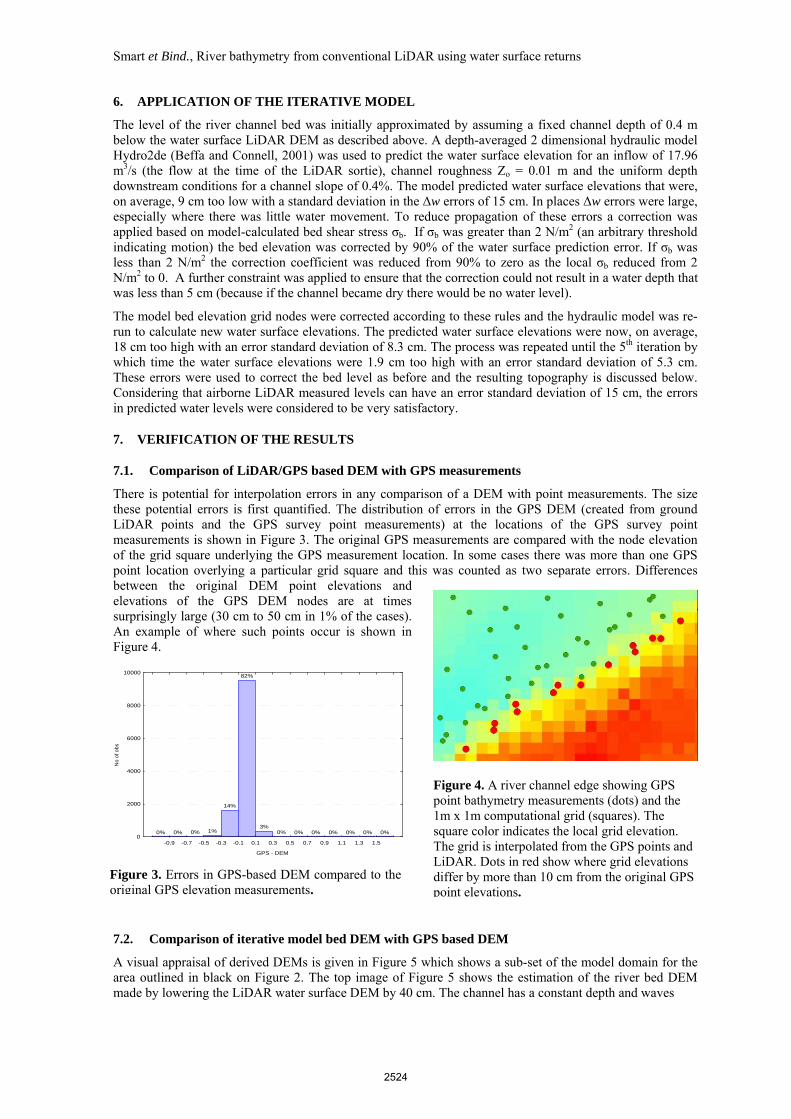
There is potential for interpolation errors in any comparison of a DEM with point measurements. The size these potential errors is first quantified. The distribution of errors in the GPS DEM (created from ground LiDAR points and the GPS survey point measurements) at the locations of the GPS survey point measurements is shown in Figure 3. The original GPS measurements are compared with the node elevation of the grid square underlying the GPS measurement location. In some cases there was more than one GPS point location overlying a particular grid square and this was counted as two separate errors. Differences between the original DEM point elevations and elevations of the GPS DEM nodes are at times surprisingly large (30 cm to 50 cm in 1% of the cases). An example of where such points occur is shown in Figure 4.

7.2. Comparison of iterative model bed DEM with GPS based DEM

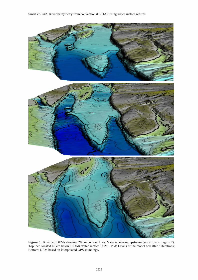
A visual appraisal of derived DEMs is given in Figure 5 which shows a sub-set of the model domain for the area outlined in black on Figure 2. The top image of Figure 5 shows the estimation of the river bed DEM made by lowering the LiDAR water surface DEM by 40 cm. The channel has a constant depth and waves

Figure 4. A river channel edge showing GPS point bathymetry measurements (dots) and the 1m x 1m computational grid (squares). The square color indicates the local grid elevation. The grid is interpolated from the GPS points and LiDAR. Dots in red show where grid elevations differ by more than 10 cm from the original GPS point elevations.

0% 0% 0% 1%

14%

82%

3%0% 0% 0% 0% 0% 0% 0%

-0.9 -0.7 -0.5 -0.3 -0.1 0.1 0.3 0.5 0.7 0.9 1.1 1.3 1.5

GPS - DEM

0

2000

4000

6000

8000

10000

No

of o

bs

Figure 3. Errors in GPS-based DEM compared to the original GPS elevation measurements.

2524

Smart et Bind., River bathymetry from conventional LiDAR using water surface returns

Figure 5. Riverbed DEMs showing 20 cm contour lines. View is looking upstream (see arrow in Figure 2). Top: bed located 40 cm below LiDAR water surface DEM; Mid: Levels of the model bed after 6 iterations; Bottom: DEM based on interpolated GPS soundings.

2525

Smart et Bind., River bathymetry from conventional LiDAR using water surface returns

transferred from the water surface are evident in the bed upstream of the underwater “island” in the centre of the image. This constant depth DEM was used as the starting point for model iterations. The middle image of Figure 5 shows levels following 6 iterations of the proposed model bed. Surface waves have gone and riffles and pools are now apparent in the bed morphology. The “island” has become more of a pointed bar and the bed displays the complexity expected in an unconstrained gravel bed river. The bottom image of Figure 5 shows the bed DEM interpolated from GPS point measurements. This should give the most accurate representation of the river bed. The image shows the “island” as a pointed bar but there is less detail than results from the iterative model. The GPS tracks shown on Figure 2 indicate that (especially in the centre of the area) there are some gaps in the measured bed data and levels in these gaps have smoothed topography that depends on the interpolation.

7.3. Analysis of errors

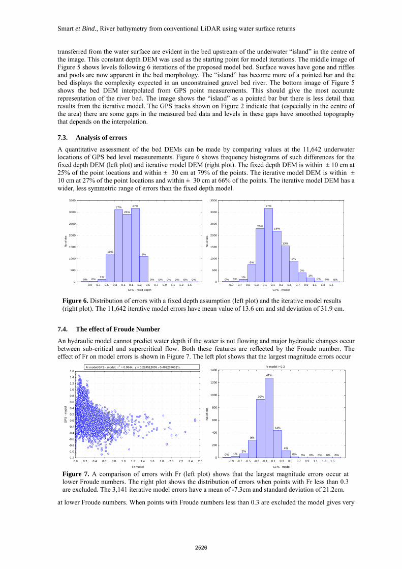
A quantitative assessment of the bed DEMs can be made by comparing values at the 11,642 underwater locations of GPS bed level measurements. Figure 6 shows frequency histograms of such differences for the fixed depth DEM (left plot) and iterative model DEM (right plot). The fixed depth DEM is within ± 10 cm at 25% of the point locations and within ± 30 cm at 79% of the points. The iterative model DEM is within ± 10 cm at 27% of the point locations and within ± 30 cm at 66% of the points. The iterative model DEM has a wider, less symmetric range of errors than the fixed depth model.

7.4. The effect of Froude Number

An hydraulic model cannot predict water depth if the water is not flowing and major hydraulic changes occur between sub-critical and supercritical flow. Both these features are reflected by the Froude number. The effect of Fr on model errors is shown in Figure 7. The left plot shows that the largest magnitude errors occur

at lower Froude numbers. When points with Froude numbers less than 0.3 are excluded the model gives very

0% 0%1%

10%

27%

25%

27%

9%

0% 0% 0% 0% 0% 0%

-0.9 -0.7 -0.5 -0.3 -0.1 0.1 0.3 0.5 0.7 0.9 1.1 1.3 1.5

GPS - fixed depth

0

500

1000

1500

2000

2500

3000

3500

No

of o

bs

0% 0%1%

6%

20%

27%

19%

13%

8%

3%

1%0% 0% 0%

-0.9 -0.7 -0.5 -0.3 -0.1 0.1 0.3 0.5 0.7 0.9 1.1 1.3 1.5

GPS - model

0

500

1000

1500

2000

2500

3000

3500

No

of o

bs

Figure 6. Distribution of errors with a fixed depth assumption (left plot) and the iterative model results (right plot). The 11,642 iterative model errors have mean value of 13.6 cm and std deviation of 31.9 cm.

Scatterplot (Sheet1 in Channel data.stw 13v*11624c)

0.0 0.2 0.4 0.6 0.8 1.0 1.2 1.4 1.6 1.8 2.0 2.2 2.4 2.6

Fr model

-1.2

-1.0

-0.8

-0.6

-0.4

-0.2

0.0

0.2

0.4

0.6

0.8

1.0

1.2

1.4

1.6

GPS

- m

odel

Fr model:GPS - model: r 2 = 0.0844; y = 0.224512655 - 0.493237652*x Fr model > 0.3

0% 1%2%

9%

30%

41%

14%

4%

0% 0% 0% 0% 0% 0%

-0.9 -0.7 -0.5 -0.3 -0.1 0.1 0.3 0.5 0.7 0.9 1.1 1.3 1.5

GPS - model

0

200

400

600

800

1000

1200

1400

No

of o

bs

Figure 7. A comparison of errors with Fr (left plot) shows that the largest magnitude errors occur at lower Froude numbers. The right plot shows the distribution of errors when points with Fr less than 0.3 are excluded. The 3,141 iterative model errors have a mean of -7.3cm and standard deviation of 21.2cm.

2526

Smart et Bind., River bathymetry from conventional LiDAR using water surface returns

good results. The error distribution (Figure 7, right plot) now shows that 41% of the predicted bed levels lie within ± 10cm of the GPS-measured bed level and 85% of the predicted levels lie within ± 30cm of the GPS-measured bed. The error distribution is Gaussian (Shapiro-Wilk W = 0.98186, p = 0.0000, mean -7.3 cm, std deviation 21.2cm). Considering that LiDAR measurements of dry topography can have an error std. deviation of 15 cm, for Fr > 0.3 the model predictions of underwater bed positions are surprisingly accurate.

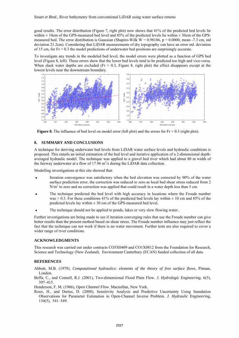
To investigate any trends in the modeled bed level, the model errors were plotted as a function of GPS bed level (Figure 8, left). These errors show that the lower bed levels tend to be predicted too high and vice-versa. When slack water depths are excluded (Fr > 0.3, Figure 8, right plot) the effect disappears except at the lowest levels near the downstream boundary.

8. SUMMARY AND CONCLUSIONS

A technique for deriving underwater bed levels from LiDAR water surface levels and hydraulic conditions is proposed. This entails an initial estimation of the bed level and iterative application of a 2-dimensional depth-averaged hydraulic model. The technique was applied to a gravel bed river which had about 80 m width of the fairway underwater at a flow of 17.96 m3/s during the LiDAR data collection.

Modelling investigations at this site showed that:

● Iteration convergence was satisfactory when the bed elevation was corrected by 90% of the water surface prediction error, the correction was reduced to zero as local bed shear stress reduced from 2 N/m2 to zero and no correction was applied that could result in a water depth less than 5 cm.

● The technique predicted the bed level with high accuracy in locations where the Froude number was > 0.3. For these conditions 41% of the predicted bed levels lay within ± 10 cm and 85% of the predicted levels lay within ± 30 cm of the GPS-measured bed level.

● The technique should not be applied to ponds, lakes or very slow flowing water..

Further investigations are being made to see if iteration converging rules that use the Froude number can give better results than the present method based on shear stress. The Froude number influence may just reflect the fact that the technique can not work if there is no water movement. Further tests are also required to cover a wider range of river conditions.

ACKNOWLEDGMENTS

This research was carried out under contracts CO5X0409 and CO1X0812 from the Foundation for Research, Science and Technology (New Zealand). Environment Canterbury (ECAN) funded collection of all data.

REFERENCES

Abbott, M.B. (1979), Computational hydraulics: elements of the theory of free surface flows, Pitman, London.

Beffa, C., and Connell, R.J. (2001), Two-dimensional Flood Plain Flow. J. Hydrologic Engineering, 6(5), 397–415.

Henderson, F. M. (1966), Open Channel Flow. Macmillan, New York. Roux, H., and Dartus, D. (2008), Sensitivity Analysis and Predictive Uncertainty Using Inundation

Observations for Parameter Estimation in Open-Channel Inverse Problem. J. Hydraulic Engineering, 134(5), 541–549.

196 197 198 199 200 201 202 203

GPS Bed Level [m]

-1.2

-1.0

-0.8

-0.6

-0.4

-0.2

0.0

0.2

0.4

0.6

0.8

1.0

1.2

1.4

1.6

GP

S -

mod

el

196 197 198 199 200 201 202 203

GPS Bed Level [m]

-1.2

-1.0

-0.8

-0.6

-0.4

-0.2

0.0

0.2

0.4

0.6

0.8

GP

S -

mod

el

Figure 8. The influence of bed level on model error (left plot) and the errors for Fr > 0.3 (right plot).

2527