arX

iv:1

703.

0003

0v1

[as

tro-

ph.I

M]

28

Feb

2017

Draft version March 2, 2017Preprint typeset using LATEX style emulateapj v. 12/16/11

IMAGE SUBTRACTION REDUCTION OF OPEN CLUSTERS M35 & NGC 2158 IN THE K2 CAMPAIGN-0SUPER-STAMP

M. Soares-Furtado1,†, J. D. Hartman1, G. A. Bakos1,*,**, C. X. Huang2, K. Penev1, W. Bhatti1

Draft version March 2, 2017

ABSTRACT

Observations were made of the open clusters M35 and NGC 2158 during the initial K2 campaign(C0). Reducing these data to high-precision photometric time-series is challenging due to the widepoint spread function (PSF) and the blending of stellar light in such dense regions. We developedan image-subtraction-based K2 reduction pipeline that is applicable to both crowded and sparsestellar fields. We applied our pipeline to the data-rich C0 K2 super-stamp, containing the two openclusters, as well as to the neighboring postage stamps. In this paper, we present our image subtractionreduction pipeline and demonstrate that this technique achieves ultra-high photometric precision forsources in the C0 super-stamp. We extract the raw light curves of 3960 stars taken from the UCAC4and EPIC catalogs and de-trend them for systematic effects. We compare our photometric results withthe prior reductions published in the literature. For detrended, TFA-corrected sources in the 12–12.25Kp magnitude range, we achieve a best 6.5 hour window running rms of 35 ppm, falling to 100ppmfor fainter stars in the 14–14.25 Kp magnitude range. For stars with Kp > 14, our detrended and 6.5hour binned light curves achieve the highest photometric precision. Moreover, all our TFA-correctedsources have higher precision on all timescales investigated. This work represents the first publishedimage subtraction analysis of a K2 super-stamp. This method will be particularly useful for analyzingthe Galactic bulge observations carried out during K2 campaign 9. The raw light curves and the finalresults of our detrending processes are publicly available at http://k2.hatsurveys.org/archive/.

Subject headings: open clusters and associations: individual (M35), (NGC 2158) — stars: variables:general — methods: data analysis – techniques: image processing, photometric-surveys -astrometry / K2

1. INTRODUCTION

Since its launch in April of 2008, the Kepler SpaceTelescope has systematically detected an unprecedentednumber of exoplanet candidates from the photometricsignatures that these sources impart as they transit theirhost stars (e.g. Mullally et al. (2015)). Undoubtedly, theKepler mission has played a pivotal role in the field ofexoplanetary science, contributing the largest catalog ofexoplanet candidates to date: 2/3rd of the current exo-planetary census data (Morton et al. 2016).The Kepler photometer is a single-purpose instrument

with a 0.95-m aperture Schmidt telescope design anda wide, ∼100-square-degree field of view (FOV). A de-tailed description of the Kepler mission can be foundin Borucki et al. (2010) and Koch et al. (2010). Duringthe primary phase of the Kepler mission, the spacecraftpointed toward a single patch of sky, simultaneously ob-serving more than 100,000 stars.In 2013, after four years of service, it was necessary to

revise the direction of the mission after the failure of thesecond gyroscopic reaction wheel, a requisite to main-tain telescope pointing stability. This event ushered inthe second phase of the mission, the K2 Ecliptic Survey

1 Department of Astrophysical Sciences, Princeton University,Princeton, NJ 08544, USA; email: msoares@astro.princeton.edu

† National Science Foundation Graduate Research Fellow∗ Alfred P. Sloan Research Fellow∗∗ Packard Fellow2 Astrophysics Department, Dunlap Institute for Astronomy

and Astrophysics, University of Toronto, Toronto,ON M5S 3H4,Canada

(K2 ), designed to exploit the solar radiation and firingof thrusters as a means of maintaining pointing preci-sion (Howell et al. 2014). K2 operations started in Juneof 2014. Remarkably, aside from the failure of the tworeaction wheels, the Kepler spacecraft exhibits little per-formance degradation and fuel budget estimates suggesta duration of 2–3 years for this second phase.K2 observes a series of target fields, known as cam-

paigns, along the plane of the ecliptic, for a span of∼75 days each. Through the numerous pointings scan-ning a multitude of Galactic coordinates, the K2 missionprovides a novel opportunity to probe transiting plan-ets among diverse stellar populations. Each individualcampaign targets ∼10,000–20,000 stars to be observedat 29-min cadence, as well as an additional ∼100 tar-gets that are observed at 1-min cadence. Observationsare also made for a number of open and globular clus-ters, including M35, NGC 2158, M4, M80, M45, NGC1647, the Hyades, M44, M67, and NGC 6717. The dataare made publicly available in a series of data releases.To date, Campaigns 0–8 have been publicly released andare available on NASA’s Barbara A. Mikulski Archive forSpace Telescopes (MAST).Our campaign of interest, C0, is the first target field,

observed during March-May 2014, and pointed towardthe dense Galactic anti-center. Approximately 22,000targets were observed in C0. Additionally, the open clus-ters M35 (NGC 2168) and NGC 2158 were observed dur-ing this campaign in what is known as a super-stamp —a contiguous aggregate of 154 separate postage stamps(50 × 50 pixels each) placed over the densest region of

2 Soares-Furtado et al.

these neighboring clusters. The open cluster M35 is ata distance of 762 ± 145 pc and has an estimated age of150Myr (McNamara et al. 2011). It is relatively sparsecompared to NGC 2158, which is at 3600 ± 400pc, and2Gyr old (Carraro et al. 2002). NGC 2158 is very dense,and was once believed to be a globular cluster.Open clusters offer an invaluable opportunity to probe

stellar and planetary astrophysics given the availabil-ity of cluster parameter constraints (e.g. age, metallic-ity, Galactic position and motion), as well as param-eters for stellar members (e.g. stellar mass and evolu-tionary state). Moreover, the age of M35 makes it anideal environment to study planetary evolution, as plan-ets are known to undergo rapid evolutionary changesduring the first few hundred million years after theirformation (Adams & Laughlin 2006). To date, onlya handful of candidate exoplanets have been found inopen clusters, primarily through radial velocity mea-surements (e.g. Sato et al. (2007); Lovis & Mayor (2007);Quinn et al. (2012); Libralato et al. (2016b)). Using theKepler satellite, Meibom et al. (2013) unveiled the firsttransiting exoplanet detection in an open cluster. Morerecently, data from the K2 mission has continued to re-veal transiting exoplanets in open cluster environments(Libralato et al. 2016b; Mann et al. 2016b,a). There re-mains much to be learned regarding this intriguing classof objects, such as whether exoplanets are a ubiquitouspresence in dense open cluster environments.In crowded open cluster fields, however, heavy blend-

ing of light from neighboring stars is unavoidable. Thisproblem is only amplified by the large pixel size, widePSF, and the lower pointing stability of the K2 mis-sion. As a result, simple aperture photometry is not anoptimal means of obtaining high-precision stellar pho-tometry. Our work aims to fully exploit the data-richK2 super-stamps using an image subtraction reductiontechnique, also known as “differential image analysis,”outlined by Alard & Lupton (1998). We fully automatethis procedure into a reduction pipeline and apply it tosources in the C0 super-stamp.There have been numerous investigations focusing on

the same data set in the past. Vanderburg (2014) derivedphotometry for C0 data using an efficient detrendingcorrection technique outlined in Vanderburg & Johnson(2014). This work focused solely on proposedKepler tar-get postage stamps, omitting cluster members and neigh-boring stars located on the C0 super-stamp. The firstvariability search on C0 target postage stamps was per-formed by Armstrong et al. (2015), also excluding theC0 super-stamp. This culminated in the identification of8395 variable sources.The first photometric results for C0 cluster mem-

bers were obtained by (Libralato et al. (2016a), hereafterL16), curtailing the averse effects of light blending byemploying a well-established PSF neighbor-subtractionmethod, known to be an effective tool for extracting high-quality time series data in dense fields, and then perform-ing aperture photometry (Montalto et al. 2007). Theyemploy the high-angular-resolutionAsiago Input Catalog(AIC), assembled from observations by the ground-basedAsiago Schmidt Telescope. This catalog lists 75,935objects in the region containing M35 and NGC 2158(Nardiello et al. 2015). While the AIC extends to faintmagnitudes of Kp ≃ 24, the rms scatter (defined as the

3.5 σ-clipped 68.27th-percentile of the distribution aboutthe median value of the light curve magnitude) for suchdim stars is on the order of 50 times greater than that ofsources in the 10–11 magnitude range. Moreover, as ourprimary aim is to search for planetary transits in denseK2 fields, we focus our sources for which reasonable pho-tometry can be retrieved (rms < 0.02).The PSF neighbor-subtraction method requires high

accuracy in the PSF modeling, otherwise the techniquewill produce false residuals and systematic errors — aconcern that our image subtraction technique circum-vents. The work of L16 resulted in a catalog of 2,133variable stars found within the C0 super-stamp.Our work provides the first image subtraction re-

duction of the C0 super-stamp, effectively removingsources with no detectable variability from the clus-ter field, therefore reducing blending, to produce high-precision differential photometry. While applying theimage subtraction reduction technique to K2 super-stamps is novel, the method itself is not a new concept.Alard & Lupton (1998) outlined this procedure nearlytwo decades ago, releasing the ISIS package and thenfurther optimizing this process by incorporating a space-varying convolution kernel (Alard 2000). We make useof the image subtraction implementation of the HATNetproject (Bakos et al. 2010) as described by Pal (2012).The crowding from variable sources and the photon-

noise residuals of non-variable sources on the image-subtracted frames is much smaller than crowding presenton the original unsubtracted frames. This is because thevast majority of photometric sources tend to be eithernot detectably variable or they are only variable overlong timescales. The image subtraction technique there-fore offers the major advantage of far less blending in theresulting photometry. Furthermore, rather than model-ing each of the images for a given cadence, we modelthe changes between images, which include variations inpointing, flux scaling, background, and the convolutionkernel relating PSFs. These variations tend to be sim-pler to accurately model and are generally well fit bysimple functions. The PSF, background, star positions,and relative fluxes are determined only once for a singlephotometric reference frame, which, in our case, is themedian valued co-added frame taken from the entiretyof our selected data set. Moreover, systematic errorsthat arise produce an increase in the overall amplitudeof a light curve (a scaling error), rather than contribut-ing to light curve noise. In contrast, proper modelingof the non-subtracted frames requires accurate modelingof the PSF, positions, background, and relative fluxes,which is far more challenging, particularly for an opencluster region where blending is profuse. One additionaladvantage of the image subtraction is that the source ofthe variation is often uniquely identified from the excess(or missing) residual flux at a given location, even understrong crowding.In this paper, we reduce data from the K2 C0 super-

stamps and neighboring target pixel files to producehigh-precision photometry for sources down to Kp ∼ 16,employing techniques developed from the HAT ground-based transit surveys (Bakos et al. 2010) and buildingupon the work of Huang et al. (2015). We publicly re-lease the raw and detrended high-precision light curves.We briefly review K2 observations and describe C0 data

K2 C0 Image Subtraction Reduced Light Curves 3

extraction in Section 2. The data reduction method isreviewed in Section 3, including astrometry, image sub-traction, and photometry. Our detrending techniques arediscussed in Section 4. Finally, in Section 5, we compareour C0 photometry and light curves with those obtainedfrom prior studies (specifically that of L16), and demon-strate that we have generated the most precise photo-metric analysis of sources in C0 super-stamp. This isfollowed by a summary of our current efforts to conducta variability search of our time series data.

2. OBSERVATIONS

2.1. K2 Data Acquisition

A thorough review of the Kepler instrument is given inThe Kepler Instrument Handbook (2009). Here we sum-marize the principal features of K2 data acquisition.The K2 photometer is comprised of a 21-module array

covering 5-square-degrees on the sky, providing ∼100-square-degree FOV. Each module contains two separate2200 × 1024 pixel CCDs for a total of ∼95 million pix-els across the array. Two of the 21 modules were notoperable when these observations were made and, morerecently, a third module has also failed. Each modulecontains 4 output channels, designated by channel num-bers 1–84. To prevent saturation, CCDs are read outevery six seconds and the data are integrated for either along 29-minute cadence or a 1-minute short cadence. Toimprove the photometric precision, images are de-focusedto produce 10 arc-second wide PSFs.In the K2 phase the spacecraft is pointed toward the

ecliptic in order to minimize the impact of solar radia-tion pressure. The still functioning two reaction wheelsrespond to the pressure exerted by solar radiation, pro-viding a close to constant pointing alignment in the yand z axes, while the thrusters are fired to correct fordrift along the x-axis every ∼ 6 hours.The coordinates of target sources in the K2 mission are

provided by the Ecliptic Plane Input Catalog (EPIC).The number of target objects is limited by the onboardstorage, compression, and downlink capabilities, as wellas the duration of the campaign. Observations of eachtarget source, also known as a Kepler Object of Interestor KOI, are downloaded once per month as a 25×25 pixelpostage stamp centered on the target, comprising 10% ofthe entire Kepler field — although some postage stampscan be as large as 50-pixels across. super-stamps areassigned a custom aperture number to serve as an iden-tifier. Also obtained are two Full Frame Images (FFI) atthe start and end of each campaign.

2.2. K2 C0 Data Extraction

Our region of interest is the C0 super-stamp contain-ing the open clusters M35 and NGC 2158, comprised of385,000 individual pixels. These data are found on a sin-gle module output channel — channel 81. We make use ofthe long, 29-min cadence observations. Our data were ob-tained as target pixel files (TPFs) from NASA’s BarbaraA. Mikulski Archive for Space Telescopes (MAST). TPFsare the time series pixel data for a particular stamp, cen-tered on a target object. Unfortunately, the first half ofthe C0 observations were conducted in coarse pointingmode, resulting in large positional variations by up to∼20 pixels (25 mas pixel−1). Therefore, we solely analyze

the second half of the data set, which has a baseline of∼31 days (1840 cadences), where fine pointing mode wasemployed and the positional variations are significantlydiminished. In contrast, the light curves generated byL16 employ the full data set.

3. DATA REDUCTION

The data reduction process employed for our imagesubtraction pipeline is based on the procedures describedby Huang et al. (2015). Here we give a brief outline, andthen discuss the process in more detail:

1. For each cadence, we employ header informationfrom the TPFs to generate a sparse frame im-age, which contains all sources observed on the K2super-stamp and adjacent stamps.

2. We perform source extraction on the stars presentin the K2 super-stamp and adjacent TPFs andfind an absolute astrometric transformation be-tween the UCAC4 catalog (RA and Dec) and theextracted (x, y) positions of the sources in theframe.

3. An astrometric reference frame is selected. We usea sharp sparse frame image with median directionalpointing.

4. We then spatially transform all sparse frame im-ages to a common astrometric reference coordinateframe. This is accomplished by finding a transfor-mation between the pixel coordinates of source cen-troids in a particular sparse frame image and theselected astrometric reference frame. This is a cru-cial step, minimizing the effect of spacecraft driftand allowing for more accurate modeling of the mo-tion of the instrument in our detrending analysis.

5. We generate a master photometric reference frame,which is a stacked median average of all availableC0 frames, after transforming to a common astro-metric frame and matching their backgrounds andPSFs.

6. Each sparse frame cadence file is matched to andthen subtracted from the photometric referenceframe, leaving behind subtracted images showingonly the variability in the field.

7. We perform photometry on the catalog projectedsources (using the absolute astrometry above).

8. We then assemble light curves for all of the sources.

9. We apply a high-pass filter to our data (us-ing 1-day binning) and perform a parameter de-correlation procedure, analogous to that outlinedby Vanderburg & Johnson (2014), to remove theremaining small, time-correlated noise from ourlight curves.

10. We then apply the Trend Filtering Algorithm.(Kovacs et al. 2005), as implemented in vartools(Hartman & Bakos 2016) to further remove sys-tematic artifacts from the data.

4 Soares-Furtado et al.

3.1. Source Catalog Preparation

Our astrometry procedure is dependent upon an inde-pendent knowledge of the true positions of the observedcelestial sources. For this, we employ the fourth editionof the United States Naval Observatory CCD AstrographCatalog (UCAC4) (Zacharias et al. 2013). This catalogis based upon observations with a much higher spatialresolution than the K2 observations and, as such, pro-vides more accurate positions and photometric measure-ments than what can be deduced from the data alone.UCAC4 covers a stellar brightness range of 8th-16thmagnitude in a single bandpass between V and R. Posi-tional errors are on the order of 15–20 mas for stars in therange 10th-14th magnitude. Measurements are based onthe International Celestial Reference System (ICRS) ata mean epoch of 2000. In addition to positional coordi-nates, the UCAC4 lists measurements of proper motionfor ∼92% of cataloged stars with errors on the order of1–10 mas yr−1. In the work performed by Huang et al.(2015), first-order corrections were applied to the coordi-nates of catalog objects based upon the proper motionsto account for positional changes.These catalogs are imperative to determining accurate

brightness measurements for sources, as they have highspatial resolution, and are therefore less impacted byblending. The UCAC4 is supplemented by photomet-ric data from the Two Micron All Sky Survey (2MASS)(Skrutskie et al. 2006) for ∼92% of cataloged stars (J,H and K bands), as well from the AAVSO PhotometricAll-Sky Survey (APASS) for ∼ 45% of objects (BVgribands).The Kepler magnitude (Kp), a measure of the source

intensity as observed through the wide Kepler bandpass,is computed for all sources using pre-existing photomet-ric data. Following the hierarchical conversion methodoutlined in Brown et al. (2011), we employ gri band pho-tometry whenever possible. For sources without thesemeasurements, however, we employ BV band magni-tudes from the Tycho-2 catalog (Høg et al. 2000). Fora subset of sources, we use B and V magnitude measure-ments to estimate Kepler magnitudes.In addition to the K2 target sources, our astromet-

ric analysis provides positions and photometry for manyother stars falling on the super-stamp and adjacent tar-get pixel files. In total, 120 of our final light curves areK2 target sources, while the remaining 3840 light curvesare for objects that are not targeted K2 sources.

3.2. Image Preparation and Astrometry

3.2.1. Sparse Frame Image Construction

We make use of the publicly available K2 C0 TPFs,generating a sparse frame image of the entire channel foreach cadence by stitching together the individual targetpixel stamps. This is a useful alternative to working witha multitude of separate target pixel stamps. We use theavailable fits header information to determine the properplacement of target pixel stamps and compare our resultswith the FFI for that same field.Each sparse frame image is comprised of a field of

1132 × 1070 square pixels, and unobserved regions inthe sparse frame image are masked. A Python script au-tomates the translation and stitching procedure, recon-structing a total of 1,392 high-quality sparse frame im-

ages in fine-pointing mode, with each image correspond-ing to an individual cadence. These frames are cross-checked with the FFI to ensure proper reconstruction.Figure 1 shows one example of a sparse frame image.

3.2.2. Relative Astrometry

The next step is a translation of each of the cadenceframes into a common reference coordinate system. Theastrometric reference file is a sparse frame image thatsets the coordinate reference frame. The astrometric ref-erence file is selected for its sharp stellar profiles, as com-pared to the other files, and a pointing position that isclose to the median pointing over the duration of theobservations.We perform source extraction on the astrometric refer-

ence frame. We use the tool fistar, available in the as-tronomical image and data processing open-source soft-ware package FITSH, to detect and extract sources fromthe images. The fistar tool designates source candi-date pixel groups, modeled in our case by an asymmetricGaussian profile in order to derive precise centroid coor-dinates and shape parameters. We then extract the PSFfor the image, based on the modeled sources. The out-put file is a list of detected and extracted sources (e.g.positions, S/N, Flux).We then employ the FITSH tool grmatch to match de-

tected sources from each of the sparse frame images tothat of the astrometric reference frame. Matching is per-formed using a 2-dimensional point matching algorithm,determining an appropriate geometrical transformationto transform the points from each sparse frame cadenceimage to the astrometric reference frame, finding as manypairs as possible (Pal & Bakos 2006).The output file contains the relevant geometrical trans-

formation and statistics regarding the quality of thetransformation. We employ an adapted version of theFITSH tool fitrans to perform the appropriate geomet-ric transformations on each of the sparse frame cadencefiles. We use linear interpolation between the pixels in-volving exact flux conservation by integrating on the im-age surface.The relative astrometry step is vital as it (a) generates

accurate centroids for sources and (b) mitigates negativeeffects introduced by the spacecraft roll, which allows formore accurate modeling of the instrument motion in ourdetrending procedure. The original Kepler mission wasknown for its excellent pointing stability, while K2 obser-vations are plagued by significant pixel drift, with a typi-cal star shifting along a ∼2-pixel long arc in our C0 dataset. Variations in the pixel sensitivity produce fluctua-tions in the measured flux as a function of centroid posi-tion. Not surprisingly, the resulting PSF is distorted andblending is recurrently inevitable, particularly in densestellar regions. Determining an accurate PSF shape isa crucial step in obtaining high-precision photometry incrowded fields like C0.

3.3. Image Subtraction

For Kepler and K2, aperture photometry is the pri-mary method employed to derive light curves. Certainregions, however, are crowded, partly due to Kepler’slarge, undersampled pixels (∼4 arcsec/pixel). Moreover,the PSF extends across several pixels. Here aperture

K2 C0 Image Subtraction Reduced Light Curves 5

photometry can perform sub-optimally. Subtracting outthe flux from non-varying sources is a means of teasingout the photometric variable sources in crowded regionsL16 used the high-resolution AIC (Asiago Input Catalog)to identify neighbors for sources in the C0 super-stampfield, subtracting out the contributions from these con-taminants.Our method, however, instead relies on the creation of

a stacked frame, coined the photo-reference frame, com-prised of all 2419 K2 C0 frames. We explored multiplemethods to generate the optimal photo-reference frameby varying the number of frames in the stack, employingquality cuts on frames included in the stack, and tryingdifferent averaging techniques. After comparing the re-sulting light curve quality and rms scatter of these routes,we conclude that the optimal photo-reference frame isgenerated by astrometrically matching our sparse frameimages with fitrans, convolving the set of frames tomatch their corresponding PSFs and backgrounds, andthen combining them to take the mean flux. We usethe ficonv tool from the FITSH package to match andconvolve the frames. We note that matching the back-grounds is particularly important due to the considerablechanges in the zodiacal background light over the cam-paign.After generating the photo-reference frame, we then

use ficonv to match the background and PSF of eachstitched frame cadence image to that of the photo-reference image before subtracting the two frames fromone another. In order to properly do this we optimizethe selected convolution kernel parameters, settling on adiscrete image subtraction kernel over a Gaussian kernel.With the frames appropriately convolved, we subtract

photo-reference frame from each of the convolved indi-vidual cadences, leaving behind a sparser stellar field ofvarying sources (and residuals left after constant stars),as shown in Figure 1.In addition to reducing blending in crowded regions,

image subtraction affords the ability to uniquely identifysources from the excess (or missing) residual flux at agiven location, even in dense stellar fields.

3.3.1. Image Subtraction Kernel

We parameterize the transformation that matches anobserved image to the photo-reference image using amodel of the form:

I ′ij =

l=OB−m∑

l=0

m=OB∑

m=0

blmiljm

+

l=OI−m∑

l=0

m=OI∑

m=0

K00lmiljm × Iij

+

l=OK−m∑

l=0

m=OK∑

m=0

i′,j′=k∑

i′,j′=−k,i′j′ 6=00

Ki′j′lmiljm

× (Ii+i′,j+j′ − Iij)/2,

where Iij represents the image undergoing analysis, I ′ijis the corresponding transformed image. The free pa-rameters blm signify changes in the background, K00lm

signify changes in the flux scaling, and Ki′j′lm, withi′j′ 6= 00, represent the discrete convolution kernel mod-

eling changes in the shape of the PSF. We use polyno-mials in the spatial coordinates (i, j) to represent spatialvariations in each of these transformations. The orderof the polynomial is given by OB , OI and OK for thebackground, flux scaling, and PSF shape changes, re-spectively. The free parameters are linearly optimized tominimize the sum ∑

ij

(I ′ij −Rij)2,

where R represents the photo-reference image. We ex-plored a variety of values for the half-size of the discreteconvolution kernel (k), and the spatial polynomial or-ders OB, OI and OK . We settled on the optimal valueof k = 2. We also found that assuming no spatial varia-tion in the parameters (OB = OI = OK = 0) generallyprovided the best results.The optimal kernel parameters for each source are

listed in the final column in Table 2 in the format“b0i0d20” (the numbers here represent example discretekernel values that produces high-quality results). Thenumber following ‘b’ represents the optimal value of OB

for that source. The value following ‘i’ sets OI . The twonumbers following ‘d’ represent k and OK , respectively.For all sources we find that the light curve scatter isminimized when adopting OI = OK = 0 and k = 2. Theoptimal value for the order of the constant offset back-ground kernel OB, however, varies on a source-by-sourcebasis, ranging between 0–4.

3.4. Photometry

There are two steps in performing photometry usingsubtracted images: 1. measuring the total fluxes of eachof the sources on the photo-reference image, and 2. mea-suring the differential fluxes of each of the sources oneach of the subtracted images. The total flux of a givensource on a given image is then the sum of the referenceflux of the source and the differential flux of the sourcefor the image in question.Determining the reference fluxes in this case is com-

plicated due to the low spatial resolution of K2 and thesignificant blending of sources in the field of these clus-ters. We therefore make use of the UCAC4 determinedK2 magnitudes, which are based on higher spatial reso-lution images, to set the relative fluxes of all sources inthe field. To determine the zero-point flux level for thephoto-reference image, we perform aperture photometryon the image using the fiphot tool in the FITSH pack-age, and then determine the median ratio of the aperturephotometry flux to the UCAC4 determined flux for un-blended sources. Note that we are assuming in this pro-cess that none of the sources have varied in brightnessbetween the UCAC4 and the photo-reference image, anyviolation of this assumption will lead to an error in theamplitude of variations in our image subtraction lightcurve, but will not distort the signal or add noise to it.Differential fluxes are also computed using fiphot. We

perform aperture photometry on the subtracted imagesat the fixed locations of the UCAC4 sources transformedto the image coordinates based on our astrometric solu-tions determined in Section 3.2. In order to ensure thatthe differential photometry is measured on a consistentsystem, fiphot makes use of the kernel parameters de-termined by ficonv to account for any changes in the

6 Soares-Furtado et al.

K2 Campaign 0 --Channel 81

Fig. 1.— K2 Campaign 0 super-stamp containing open clusters M35 and NGC 2158. The figure is generated by stitching stamps withina given channel (channel 81 in this case) into a composite image. The empty regions represent null pixels, as the information from thesepixels are not downloaded by the spacecraft. The left panel displays the raw composite frame before our image subtraction reductionpipeline is applied. The right panel is an example of a single subtracted frame for an arbitrary cadence. Variable sources remain in thesubtracted frame as well as bright stars that are still visible due to saturation or Poisson noise.

PSF shape or flux scale between the photo-reference andthe subtracted image. We employ 9 apertures to mea-sure the residual (differential) flux, ranging in size from2.5 pixels to 5.0 pixels. The suggested optimal aperturefor each source is then determined on a source-by-sourcebasis, selecting the aperture with the lowest rms for eachlight curve.

4. LIGHT CURVE DETRENDING

While the image subtraction procedure should in prin-ciple correct for systematic variations in the images, leav-ing clean light curves free of instrumental variations, wefound that, in practice, systematic variations remain, andpost-processing is needed to remove these variations. Asdescribed in Section 2.1, the low frequency roll of thesatellite causes sources to drift across the FOV. Thrustersare fired on timescales of ∼ 6 hours to correct for thiseffect. This drift results in decreased photometric pre-cision, as the star dithers between pixels changes in thepixel sensitivity must be taken into account. Fortunatelythis drift occurs largely along a single axis in a well de-fined motion, which greatly simplifies the necessary cor-rections.

There are several methods that have been employedto correct for systematic effects in K2 data. These in-clude a Gaussian process detrending approach outlinedby Aigrain et al. (2015) as well as a method discussed inForeman-Mackey et al. (2015), which performs simulta-neous fit for systematics. We follow a procedure similarto the self flat-fielding detrending method outlined byVanderburg & Johnson (2014), coined ‘K2SFF’, whichcorrects for drift systematics by decorrelating photomet-ric light curves with the spacecraft motion.The first step of our automated detrending procedure

is a culling process whereby we remove all low-qualitycadences. In the future, we plan to apply weights toeach cadence rather than simply omitting a file from thedata set. Our detrending method differs from that ofVanderburg & Johnson (2014) in that we do not relyon thruster flags labels as an indicator of file quality.Instead, we calculate the cadence-by-cadence drift be-tween source centroids, clipping cadences where the driftexceeds 3.5 σ. This method has an 82% overlap withthruster flagged cadences.From this point, a median high-pass filter is applied

to the culled data with binning windows of ∼ 1 day.

K2 C0 Image Subtraction Reduced Light Curves 7

Principal component analysis is then performed on the2-dimensional scatter traced out by the source centroidsas they drift with the spacecraft roll. This scatter isprimarily 1-dimensional, and we therefore solely utilizethe predominant basis vector. Corrections to account forchanges in pixel response as a function of arclength offset(calculated as per Vanderburg & Johnson 2014) are ap-plied. To apply the correction, we break up the predom-inant basis vector into 20 equally sized arclength offsetbins, determining the median flux for each arclength bin.We then fit a B-spline function to the binned arclengthoffset vs. median flux curve.The results of our detrending procedure can be seen

in the light curves shown in Figure 2. This figure isdiscussed in greater detail in Section 5.

4.1. Trend Filtering Algorithm

In addition to the detrending process outlined above,we also include an optional post-processing step withthe application of the Trend Filtering Algorithm (TFA),which is explained in detail in Kovacs et al. (2005). Weemploy 141 TFA template stars, which are randomly cho-sen detrended light curve files containing more than 99%of all cadences.The TFA technique, when applied in non-

reconstructive mode as we do here, may not workwell for long-period and/or high S/N variables. Insteadof filtering out purely instrumental systematic variationsor uncorrelated noise, the TFA will suppress and distortreal variability from the source. For these high S/Nand long period variables the non-TFA detrended lightcurves are optimal. The TFA does optimize our resultsfor low S/N variables — where the signal is lower thanthe effect produced by instrumental systematics, as inthis case the instrumental noise will be suppressed andthe signal is more easily identified. If the magnitudevariation is dominated by white noise, the TFA hasnegligible impact on the resulting light curve.

5. RESULTS AND DISCUSSION

In this paper we have presented our image subtrac-tion technique to generate high-precision, detrended lightcurves for stars in the open clusters M35 and NGC 2158,observed in the Campaign 0 K2 field.As L16 has already addressed a direct comparison be-

tween the neighbor-subtracted light curves and thosegenerated in Vanderburg (2014), and since Vanderburg(2014) ignores the crowded super-stamp, we compare ourresults only with L16 to determine the robustness of themethod.Figure 2 compares our light curves to those of L16

for three representative variable sources identified by theL16 variable search. In general, the image subtractionlight curves are comparable to those generated by L16using neighbor subtraction, although in selected casesour precision is superior.In addition to comparing individual sources, the top

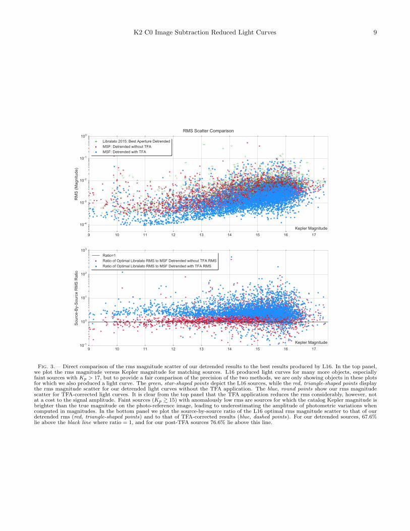
panel of Figure 3 shows the light curve rms scatter (at ca-dence) vs. Kepler magnitude for our pre-TFA detrendedlight curves, our post-TFA light curves, and the bestaperture light curves from L16, to provide the readerwith a sense of how these methods compare. The bot-tom panel shows the source-by-source ratio of the rmsscatter of the L16 derived light curves our light curves

as a function of magnitude. For our detrended sources,67.6% lie above the black Ratio = 1 line, and for ourpost-TFA sources 76.6% lie above this line, indicating areduction in the light curve rms, which does not come ata cost to the signal amplitude.In the top panel of Figure 4 we show the same results

after binning the light curves by 6.5 hr, and in the thirdpanel we show the results when computing the 6.5 hrrunning-window rms as defined by Vanderburg (2014)(this is computed to allow a more direct comparisonto prior results, and is calculated by dividing the long-cadence light curves into bins of 13 consecutive cadences,computing the rms in each bin and dividing by

√13, and

then taking the median value over all bins). The sec-ond and fourth panels of Figure 4 display the source-by-source ratios (L16 to our data set) of the 6.5 hr binnedrms and 6.5 hr running window rms (using only qualityflagged data), respectively. We determine the ratios forboth our detrended results and the TFA-corrected re-sults.We find that our pre-TFA detrended light curves are

comparable to those of L16 (with a small improvementfor fainter stars with Kp > 14mag), while the post-TFA light curves have substantially less scatter on alltimescales investigated. Part of this is due to the filteringby TFA of real stellar variability which is very commonamong the stars in these observations, however some ofthis is also due to the power of TFA at removing instru-mental systematics. Figure 5 shows the median autocor-relation function of the light curves of bright sources with11 < KP < 12. We find that while power at the 6 hr rollfrequency is substantially reduced in the detrended lightcurve autocorrelation function, compared to what is seenfor the raw light curves, there still remains a clear sig-nature of these systematics even in the detrended lightcurves. This signal is completely removed in the TFAlight curves, and the data are essentially uncorrelated intime.For stars with Kp > 14 our detrended and 6.5 hour

binned light curves achieve the highest precision to datefor the C0 super-stamp. Post-processing of these lightcurves is still needed to remove systematics and searchfor small transiting planets. This work represents thefirst published image subtraction analysis of a K2 super-stamp. This method will provide a valuable means ofanalysis of the Galactic Bulge observations carried outduring K2 campaign 9.We make the subtracted images, raw light curves,

and detrended light curves generated from the K2 C0super-stamp publicly available at the HAT data server:http://k2.hatsurveys.org/archive/. The light curvefiles contain the following information: time of observa-tion, cadence number, subtracted and detrended fluxesand associated errors for several apertures, raw relativefluxes and associated errors, centroid positions, and theaccompanying PSF kernel parameters for our best re-sulting light curve. The format of the light curve files isgiven in Tables 1 and 2, for the detrended results (con-taining the data for the raw light curves therein) and thedetrended with TFA light curves, respectively. Missingfrom Table 2 (in order to save space and omit redun-dancy) are the columns listing the raw and detrended rmsvalues associated with all 9 possible apertures. We also

8 Soares-Furtado et al.

1940 1945 1950 1955 1960 1965 1970Time (BJD-2454833)−0.03

−0.02

−0.01

0.00

0.01

0.02

0.03

0.04

Del

ta M

agni

tude

Libralato LC #023010

Libralato 2015: Detrended 3-pixel Aperture PhotometryMSF: Raw LCMSF: Detrended without TFA

1940 1945 1950 1955 1960 1965 1970Time (BJD-2454833)

−0.10

−0.05

0.00

0.05

0.10

Del

ta M

agni

tude

Libralato LC #005633

1940 1945 1950 1955 1960 1965 1970Time (BJD-2454833)

−0.10

−0.05

0.00

0.05

0.10

Del

ta M

agni

tude

Libralato LC #028459

Fig. 2.— Direct comparison of our photometric results with known variable sources presented in L16. The green, star-shaped pointsillustrate the best aperture detrended results produced by L16 (these happen to be the detrended three-pixel aperture photometric results),while the purple, round points show our raw, image-subtracted, best aperture results for the same source. The red, triangle-shaped pointsdisplay our detrended, best aperture photometric results without application of the TFA procedure. In both the top and middle panels,our results are comparable to that of L16, while in the bottom panel both our raw and detrended light curve show far less scatter.

K2 C0 Image Subtraction Reduced Light Curves 9

9 10 11 12 13 14 15 16 17

Kepler Magnitude10-4

10-3

10-2

10-1

100

RM

S (M

agni

tude

)

RMS Scatter Comparison

Libralato 2015: Best Aperture DetrendedMSF: Detrended without TFAMSF: Detrended with TFA

9 10 11 12 13 14 15 16 17

Kepler Magnitude10-1

100

101

102

103

Sou

rce-

By-

Sou

rce

RM

S R

atio

Ratio=1Ratio of Optimal Libralato RMS to MSF Detrended without TFA RMSRatio of Optimal Libralato RMS to MSF Detrended with TFA RMS

Fig. 3.— Direct comparison of the rms magnitude scatter of our detrended results to the best results produced by L16. In the top panel,we plot the rms magnitude versus Kepler magnitude for matching sources. L16 produced light curves for many more objects, especiallyfaint sources with Kp > 17, but to provide a fair comparison of the precision of the two methods, we are only showing objects in these plotsfor which we also produced a light curve. The green, star-shaped points depict the L16 sources, while the red, triangle-shaped points displaythe rms magnitude scatter for our detrended light curves without the TFA application. The blue, round points show our rms magnitudescatter for TFA-corrected light curves. It is clear from the top panel that the TFA application reduces the rms considerably, however, notat a cost to the signal amplitude. Faint sources (Kp & 15) with anomalously low rms are sources for which the catalog Kepler magnitude isbrighter than the true magnitude on the photo-reference image, leading to underestimating the amplitude of photometric variations whencomputed in magnitudes. In the bottom panel we plot the source-by-source ratio of the L16 optimal rms magnitude scatter to that of ourdetrended rms (red, triangle-shaped points) and to that of TFA-corrected results (blue, dashed points). For our detrended sources, 67.6%lie above the black line where ratio = 1, and for our post-TFA sources 76.6% lie above this line.

10 Soares-Furtado et al.

9 10 11 12 13 14 15 16 17Kepler Magnitude10-5

10-4

10-3

10-2

10-1

100

RMS (M

agnitude

)RMS 6.5-Hour Binned Scatter Comparison

Libralato: Best Aperture RMS of the 6.5-hour binned detrended light curveMSF: RMS of the 6.5 hour binned detrended without TFA light curveMSF: RMS of the 6.5 hour binned detrended with TFA light curve

9 10 11 12 13 14 15 16 17Kepler Magnitude10-1

100

101

102

103

Sou

rce-By-Sou

rce RMS Ratio

Ratio=1Ratio of Optimal Libralato RMS to MSF Detrended with TFA RMSRatio of Optimal Libralato RMS to MSF Detrended without TFA RMS

9 10 11 12 13 14 15 16 17Kepler Magnitude10-5

10-4

10-3

10-2

10-1

100

RMS (M

agnitude

)

RMS 6.5-Hour Running Window Scatter Comparison

Libralato: Best Aperture RMS of the 6.5-hour running window detrended light curveMSF: RMS of the 6.5 hour running window detrended light curveMSF: RMS of the 6.5 hour running window detrended and TFA applied light curve

9 10 11 12 13 14 15 16 17Kepler Magnitude10-1

100

101

102

103

Sou

rce-By-Sou

rce RMS Ratio

Ratio=1Ratio of Optimal Libralato RMS to MSF Detrended with TFA RMSRatio of Optimal Libralato RMS to MSF Detrended without TFA RMS

Fig. 4.— Direct comparison of the 6.5 hour binned rms magnitude scatter of our detrended and TFA-corrected results to the best L16results in the top panel. The green, star-shaped points depict the 6.5 hour binned rms of the magnitude for all the L16 sources. The red,triangle-shaped points display our 6.5 binned rms magnitude scatter for detrended results without TFA, while the blue, circle-shaped pointsillustrate the magnitude scatter for results that are TFA-corrected. For a fair comparison, we do not show all L16 sources, and insteaddisplay only source matches between both data sets. The second panel from the top shows the source-by-source ratio of the L16 rms to ourresults for both the detrended results (red, triangle-shaped points) and the TFA-corrected results (blue, round points). The solid black linedisplays where ratio = 1. The third panel illustrates a comparison of the 6.5 hour running window rms magnitude scatter of our detrendedand TFA-corrected results to that of L16. Once again, green, star-shaped points depict L16 sources, red, triangle-shaped points representour detrended sources without TFA, and blue, circle-shaped points depict our TFA-corrected sources. In the bottom panel, we plot thesource-by-source ratio of the L16 6.5 hour running window rms to our results for both the detrended results (red, triangle-shaped points)and the TFA-corrected results (blue, round points). The solid black line displays where ratio = 1. It is worth repeating that the reducedscatter in our light curves does not come at a cost of the signal amplitude.

K2 C0 Image Subtraction Reduced Light Curves 11

-1

0

1

2

3

4

5

6

0 0.2 0.4 0.6 0.8 1

Aut

ocor

rela

tion

Time Lag [days]

Median Light-Curve Autocorrelation 11 < Kp < 12

MSF: Raw Light CurvesMSF: Detrended Light Curves

MSF: TFA Light Curves

Fig. 5.— Median discrete autocorrelation function for sourceswith 11 < Kp < 12, shown separately for our raw light curves,detrended light curves, and TFA-corrected light curves. The auto-correlation is computed relative to the formal photometric uncer-tainties. Values above unity indicate a co-variance exceeding theformal expected variance at zero lag. The raw light curves showclear periodicity at the 6 hr (0.25 day) spacecraft roll period. Thisperiodicity is suppressed in the detrended light curves, but is stillevident. The TFA light curves are effectively uncorrelated in time,and show no evidence for the 6 hr instrumental periodicity.

submit our results to the Barbara A. Mikulski Archivefor Space Telescopes (MAST) to share them with thescientific community.It is our hope that there will be continued improve-

ments of the detrending methods and photometric anal-ysis so that the C0 super-stamp may be exploited to itsfullest potential, including searching the data for vari-able sources, which will be the subject of future work.In is paper we have taken the first step of demonstratingthat the image subtraction method is capable of produc-ing light curves from K2 super-stamps with a precisionthat is comparable to that of the best method demon-strated to date. We note that L16 have independentlydetrended light curves and conducted a variable searchon M35 and NGC 2158 cluster members resulting in alist of 2133 variables. For the clusters studied here wedo not expect a significantly different yield of variablesfrom our reduction as the light curves we have generatedare of comparable precision to those of L16.We are currently working on extending this pipeline to

other crowded regions in the K2 field, particularly Cam-paign 9, which points toward the dense Galactic Center.We also aim to apply the pipeline to searching for vari-ables in globular clusters. It is likely that image subtrac-tion will perform significantly better than the neighbor-subtraction method of L16 for these particularly crowdedregions. K2 observations have been made for a numberof open and globular clusters, including M4, M80, M45,NGC 1647, the Hyades, M44, M67, and NGC 6717. Weaim to fully exploit these data-rich fields using our imagesubtraction reduction pipeline in pursuit of new intrinsicvariables and transiting planets.

Acknowledgments— MSF gratefully acknowledges thegenerous support from the National Science Foundation.The data in this paper were collected by the Ke-

pler mission, which is funded by the NASA Science

Mission directorate. The data were downloaded fromthe Barbara A. Mikulski Archive for Space Telescopes(MAST), a NASA-funded project providing astronomicaldata archives and stationed at Space Telescope ScienceInstitute (STScI). STScI is operated by the Associationof Universities for Research in Astronomy, Inc.

12

Soares-F

urta

doet

al.

TABLE 1Detrended + TFA Light Curve Format

Cadence Time Detrended Best Ap Detrended Error Best Ap Raw Best Ap x-coord y-coord TFA Detrended Best ApDays: BJD-2454833 Mag Normalized Mag Mag Image Coords Image Coords Mag Normalized

2200 1940.47759875 -0.00301 0.00813 13.96333 356.073 467.058 -0.00042201 1940.49803044 -0.00332 0.00813 13.96244 356.053 467.046 0.000252202 1940.51846192 -0.00279 0.00814 13.96163 356.017 467.038 0.000452203 1940.53889351 -0.00135 0.00814 13.96259 356.02 467.017 0.002272204 1940.5593252 0.00109 0.00813 13.96381 356.003 466.994 0.00182205 1940.57975669 -0.00941 0.00811 13.95302 355.987 466.985 -0.008642206 1940.60018828 0.00453 0.00815 13.96619 355.954 466.941 0.001542209 1940.66148304 0.0018 0.00817 13.9583 356.476 467.345 -0.00152210 1940.68191473 0.00349 0.00819 13.96045 356.454 467.354 -0.000512211 1940.70234632 0.00448 0.00821 13.96247 356.45 467.32 0.00134

K2C0Im

ageSubtra

ctionReduced

LightCurves

13

TABLE 2Detrended Without TFA Light Curve Format

Time Cadence Detrended Best Ap Error Best Ap Raw Best Ap x-coord y-coord Arclength Param Optimal PSF KernelDays: BJD-2454833 Mag Normalized Mag Mag Image Coords Image Coords Image Coords b-i-d–

1940.4776 2200 -0.00301 0.00813 13.96333 356.073 467.058 0.6232 b0i0d201940.498 2201 -0.00332 0.00813 13.96244 356.053 467.046 0.6458 –1940.5185 2202 -0.00279 0.00814 13.96163 356.017 467.038 0.6793 –1940.5389 2203 -0.00135 0.00814 13.96259 356.02 467.017 0.6899 –1940.5593 2204 0.00109 0.00813 13.96381 356.003 466.994 0.7174 –1940.5798 2205 -0.00941 0.00811 13.95302 355.987 466.985 0.7355 –1940.6002 2206 0.00453 0.00815 13.96619 355.954 466.941 0.7885 –1940.6615 2209 0.0018 0.00817 13.9583 356.476 467.345 0.1287 –1940.6819 2210 0.00349 0.00819 13.96045 356.454 467.354 0.1405 –1940.7023 2211 0.00448 0.00821 13.96247 356.45 467.32 0.1638 –

14 Soares-Furtado et al.

REFERENCES

Adams, F. C., & Laughlin, G. 2006, ApJ, 649, 1004Aigrain, S., Hodgkin, S. T., Irwin, M. J., Lewis, J. R., & Roberts,

S. J. 2015, MNRAS, 447, 2880Alard, C. 2000, A&AS, 144, 363Alard, C., & Lupton, R. H. 1998, ApJ, 503, 325Armstrong, D. J., Kirk, J., Lam, K. W. F., et al. 2015, A&A, 579,

A19Bakos, G. A., Torres, G., Pal, A., et al. 2010, ApJ, 710, 1724Borucki, W. J., Koch, D., Basri, G., et al. 2010, Science, 327, 977Brown, T. M., Latham, D. W., Everett, M. E., & Esquerdo, G. A.

2011, AJ, 142, 112Carraro, G., Girardi, L., & Marigo, P. 2002, MNRAS, 332, 705Foreman-Mackey, D., Montet, B. T., Hogg, D. W., et al. 2015,

ApJ, 806, 215

Hartman, J. D., & Bakos, G. A. 2016, Astronomy andComputing, 17, 1

Høg, E., Fabricius, C., Makarov, V. V., et al. 2000, A&A, 355, L27Howell, S. B., Sobeck, C., Haas, M., et al. 2014, PASP, 126, 398Huang, C. X., Penev, K., Hartman, J. D., et al. 2015, MNRAS,

454, 4159Koch, D. G., Borucki, W. J., Basri, G., et al. 2010, ApJ, 713, L79Kovacs, G., Bakos, G., & Noyes, R. W. 2005, MNRAS, 356, 557Libralato, M., Bedin, L. R., Nardiello, D., & Piotto, G. 2016a,

MNRAS, 456, 1137Libralato, M., Nardiello, D., Bedin, L. R., et al. 2016b, MNRASLovis, C., & Mayor, M. 2007, A&A, 472, 657

Mann, A. W., Gaidos, E., Vanderburg, A., et al. 2016a, ArXive-prints, 1609.00726

Mann, A. W., Gaidos, E., Mace, G. N., et al. 2016b, ApJ, 818, 46McNamara, B. J., Harrison, T. E., McArthur, B. E., & Benedict,

G. F. 2011, AJ, 142, 53Meibom, S., Torres, G., Fressin, F., et al. 2013, Nature, 499, 55Montalto, M., Piotto, G., Desidera, S., et al. 2007, A&A, 470,

1137Morton, T. D., Bryson, S. T., Coughlin, J. L., et al. 2016, ApJ,

822, 86Mullally, F., Coughlin, J. L., Thompson, S. E., et al. 2015, ApJS,

217, 31Nardiello, D., Bedin, L. R., Nascimbeni, V., et al. 2015, MNRAS,

447, 3536Pal, A. 2012, MNRAS, 421, 1825

Pal, A., & Bakos, G. A. 2006, PASP, 118, 1474Quinn, S. N., White, R. J., Latham, D. W., et al. 2012, ApJ, 756,

L33Sato, B., Izumiura, H., Toyota, E., et al. 2007, ApJ, 661, 527Skrutskie, M. F., Cutri, R. M., Stiening, R., et al. 2006, AJ, 131,

1163van Cleve, J. E., & Caldwell, D. 2009, Kepler Instrument

Handbook, Tech. Rep. KSCI-19033-001Vanderburg, A. 2014, ArXiv e-prints, 1412.1827Vanderburg, A., & Johnson, J. A. 2014, PASP, 126, 948Zacharias, N., Finch, C. T., Girard, T. M., et al. 2013, AJ, 145, 44