arX

iv:1

510.

0196

4v1

[as

tro-

ph.E

P] 7

Oct

201

5to appear in ApJPreprint typeset using LATEX style emulateapj v. 08/22/09

INFLUENCE OF STELLAR MULTIPLICITY ON PLANET FORMATION. IV. ADAPTIVE OPTICSIMAGING OF KEPLER STARS WITH MULTIPLE TRANSITING PLANET CANDIDATES

Ji Wang1, Debra A. Fischer1, Ji-Wei Xie2, David R. Ciardi3,(Received; Accepted)

to appear in ApJ

ABSTRACT

The Kepler mission provides a wealth of multiple transiting planet systems (MTPS). Theformation and evolution of multi-planet systems are likely to be influenced by companionstars given the abundance of multi stellar systems. We study the influence of stellar compan-ions by measuring the stellar multiplicity rate of MTPS. We select 138 bright (KP < 13.5)Kepler MTPS and search for stellar companions with AO imaging data and archival radialvelocity (RV) data. We obtain new AO images for 73 MTPS. Other MTPS in the samplehave archival AO imaging data from the Kepler Community Follow-up Observation Program(CFOP). From these imaging data, we detect 42 stellar companions around 35 host stars.For stellar separation 1 AU < a < 100 AU, the stellar multiplicity rate is 5.2 ± 5.0% forMTPS, which is 2.8σ lower than 21.1±2.8% for the control sample, i.e., the field stars in thesolar neighborhood. We identify two origins for the deficit of stellar companions within 100AU to MTPS: (1) a suppressive planet formation, and (2) the disruption of orbital copla-narity due to stellar companions. To distinguish between the two origins, we compare thestellar multiplicity rates of MTPS and single transiting planet systems (STPS). However,current data are not sufficient for this purpose. For 100 AU < a < 2000 AU, the stellarmultiplicity rates are comparable for MTPS (8.0±4.0%), STPS (6.4±5.8%), and the controlsample (12.5± 2.8%).Subject headings:

1. INTRODUCTION

As exoplanet surveys reach higher sensitivityand longer time baseline, more exoplanets are be-ing discovered. Many of these exoplanets arein multi-planet systems. As of September 2015,the radial velocity (RV) technique and the transitmethod have detected 152 and 857 planets in multi-planet systems (http://exoplanets.org, Han et al.2014). From these systems, we can study their or-bital spacing (e.g., Wright et al. 2011; Burke et al.2014), mutual inclination (e.g., Lissauer et al. 2011;Tremaine & Dong 2012), and eccentricity distribu-tion (e.g., Juric & Tremaine 2008; Kane et al. 2012;Xie 2015). These studies can be used to testtheories of planet formation and dynamical evolu-tion (Winn & Fabrycky 2015).While only ∼20% of Kepler planet host stars are

multiple transiting planet systems (MTPS), the to-tal number of planets in MTPS accounts for almosthalf of the Kepler planet candidates. Latham et al.(2011) compared Kepler MTPS to single transit-ing planet systems (STPS). They found a lackof gas giant planets in MTPS, which indicatesthat the existence of a gas giant planet may dis-rupt the orbital inclinations or suppress the forma-

Electronic address: ji.wang@yale.edu1 Department of Astronomy, Yale University, New Haven,

CT 06511 USA2 Department of Astronomy & Key Laboratory of Modern

Astronomy and Astrophysics in Ministry of Education, Nan-jing University, 210093, China

3 NASA Exoplanet Science Institute, Caltech, MS 100-22,770 South Wilson Avenue, Pasadena, CA 91125, USA

tion of multiple planets. Furthermore, other stud-ies implied that the distributions of orbital spac-ings (Xie et al. 2014), eccentricities (Xie 2015) andobliquities (Morton & Winn 2014) are different forSTPS and MTPS. In this paper, we investigate onepossibility that causes the different orbital architec-ture between STPS and MTPS, namely, the influ-ence of dynamically-bound companion stars.By comparing stellar multiplicity rate for 138

MTPS against stars in the solar neighbor-hood (Raghavan et al. 2010; Duquennoy & Mayor1991), Wang et al. (2014b) found evidence of sup-pressive planet formation in multiple stellar systemswith stellar separations smaller than 20 AU. Be-yond 20 AU, the stellar multiplicity rate was dif-ficult to measure without high resolution and deepimaging data that provide sensitivity to stellar com-panions at these separations. Therefore, at sep-arations wider than 20 AU, the influence of stel-lar companions on multi-planet formation was notwell understood. In this paper, we gather adap-tive optics (AO) images for the same MTPS samplein Wang et al. (2014b). Since AO images for 65MTPS are already available from the Kepler Com-munity Follow-up Observation Program4 (CFOP),we obtain new AO images for the remaining 73MTPS at Keck observatory and Palomar observa-tory. The archival and newly obtained AO imagesreveal dozens of new stellar companions to planethost stars and put valuable constraints on multi-planet formation in multiple stellar systems.

4 https://cfop.ipac.caltech.edu

2 Wang

The paper is organized as follows. We describethe sample selection and AO data acquisition in §2,followed by data analyses in §3. We report the stel-lar multiplicity rate for MTPS in §4. Discussion andsummary are given in §5.

2. SAMPLE DESCRIPTION AND AO DATAACQUISITION

2.1. Sample Description

The sample of MTPS remains the same as thatin Wang et al. (2014b). From the NASA Exo-planet Archive5, we select Kepler Objects of Interest(KOIs) that satisfy the following criteria: (1), dispo-sition of either Candidate or Confirmed; (2), with atleast two planet candidates; (3), Kepler magnitude(KP ) brighter than 13.5. The above selection cri-teria resulted in 138 MTPS in Wang et al. (2014b).With the updated Exoplanet Archive, the selectioncriteria resulted in 208 MTPS. In this paper, we fo-cus on the 138 MTPS to be consistent with previouswork. Their stellar and orbital parameters can befound in Table 2 and Table 3 in Wang et al. (2014b).Most MTPS in our sample are true plane-

tary systems based on a statistical analysis byLissauer et al. (2012). Subsequent papers on KeplerMTPS validated 851 planet candidates in 340 sys-tems (Rowe et al. 2014; Lissauer et al. 2014), 66MTPS in our sample are included in those vali-dated systems. Furthermore, 25 additional MTPSin our sample are confirmed planetary systems andthe remaining 47 MTPS have disposition of planetcandidate according to the latest NASA ExoplanetArchive. Therefore, the false positive rate for theMTPS sample studied in this paper should be ex-tremely low.

2.2. AO Data Acquisition

2.2.1. Archival AO Data For Follow-up Observations

We checked the continually updated CFOP. Toavoid repeated AO observations, we only observedKOIs that did not received AO follow-up observa-tions. Some of the KOIs without AO data mayhave speckle imaging (e.g., Horch et al. 2012, 2014)or lucky imaging data (e.g., Lillo-Box et al. 2012,2014), but we re-observed these KOIs at Palomarand Keck Observatory because near infrared AO im-ages provide deeper sensitivity and/or higher spa-tial resolution. For the same reason, we re-observedKOIs that have been observed by the Robo-AOproject (Law et al. 2014). For those KOIs whoseAO data from Palomar, MMT, or Keck telescopewere available through CFOP, we used the archivalAO data. In total, AO data for 65 KOIs were ob-tained from CFOP and AO data for 73 KOIs wereobtained by new observations at Palomar and Keckobservatory.

2.2.2. AO Imaging with PHARO at Palomar

We observed 68 KOIs in the sample withthe PHARO instrument (Brandl et al. 1997;Hayward et al. 2001) at the Palomar 200-inch

5 http://exoplanetarchive.ipac.caltech.edu

telescope (San Diego County, California, UnitedStates). The observations were made between UTJuly 13rd and 17th in 2014 with seeing varyingbetween 1.0′′ and 2.5′′. PHARO is behind thePalomar-3000 AO system, which provides a on-skyStrehl of 86% in K band (Burruss et al. 2014). Thepixel scale of PHARO is 25 mas pixel−1. With amosaic 1K ×1K detector, the field of view (FOV) is25′′×25′′. We normally obtained the first image inK band with a 5-point dither pattern, which had athrow of 2.5′′. AO images in K band provide highersensitivity to bound companions with late spectraltype than J and H band images. Furthermore,the AO correction in K band is better and offers abetter characterized point spread function (PSF).This is because image quality improves towardslonger wavelength for a given wavefront sensingand correcting error (Davies & Kasper 2012). Abetter image with a more stable PSF facilitatescompanion detection and characterization. Expo-sure time was set such that the peak flux of theKOI is at least 10,000 ADU for each frame, which iswithin the linear range of the detector. If a stellarcompanion was detected, we observed the KOI inJ and H bands right after the K band observation.The color information is useful for estimating thestellar properties of the stellar companion anddetermining whether the companion is physicallybound (see §3.2). Nearly simultaneous J , H , andK band observations help to minimize the influenceof any time variability of the target.

2.2.3. AO Imaging with NIRC2 at Keck II

We observed 5 KOIs in the sample with theNIRC2 instrument (Wizinowich et al. 2000) at theKeck II telescope (Mauna Kea, Hawaii, UnitedStates). The observations were made on UT July18th and August 18th in 2014 with excellent/goodseeing between 0.3′′ to 0.8′′. NIRC2 is a near in-frared imager designed for the Keck AO system.We selected the narrow camera mode, which hasa pixel scale of 10 mas pixel−1. The FOV is thus10′′×10′′ for a mosaic 1K ×1K detector. We startedthe observation in K band for each KOI for thesame reason stated in §2.2.2 and followed by J andH band observations if any stellar companions werefound. The exposure time setting is the same asthe PHARO observation: we ensured that the peakflux is at least 10,000 ADU for each frame. Weused a 3-point dither pattern with a throw of 2.5′′.We avoided the lower left quadrant in the ditherpattern because it has a much higher instrumentalnoise than the other 3 quadrants on the detector.

3. DATA ANALYSES

3.1. Contrast Curve and Detections

The raw data were processed using standard tech-niques to replace bad pixels, subtract dark, flat-field, subtract sky background, align and co-addframes. We constructed a bad pixel map usingdark frames. Pixels with dark current that deviatedmore than 5-σ from their surrounding pixels wererecorded as bad pixels. Their values were replaced

3

with the median flux of surrounding pixels. Darkframes were obtained with the exact same settingas the science frames, e.g., exposure time, co-adds,and read-out mode. After dark subtraction, eachscience frame was corrected for flat fielding. Thedithered science frames provided an estimate of thesky background which was subtracted off from thescience frames. The dark-subtracted, flat-fielded,sky-removed science frames were then co-added, re-sulting in a single frame for subsequent analyses.We calculated 5σ detection limit as follows. We

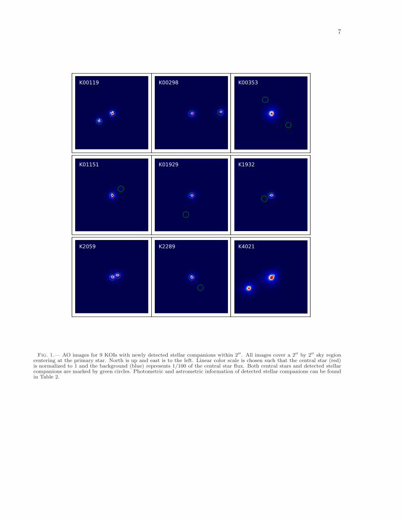
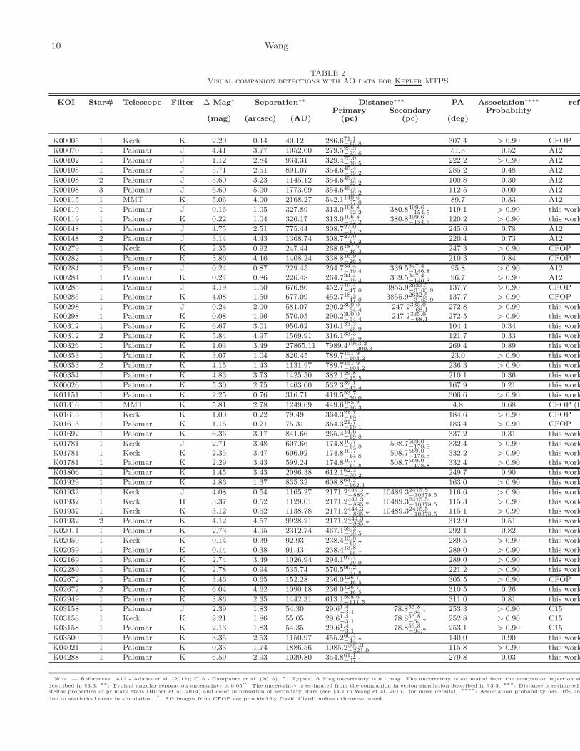
defined a series of concentric annuli centering onthe star. For the concentric annuli, we calculatedthe median and the standard deviation of flux forpixels within these annuli. We used the value of fivetimes the standard deviation above the median asthe 5σ detection limit. The detection limits at dif-ferent angular separations are reported in Table 1.We developed an automatic program to detect stel-lar companions whose differential magnitudes arebrighter than the 5-σ detection limit. The pro-gram recorded the differential magnitude, position,position angle, detection significance of each detec-tion. All detections were then visually checked toremove confusions such as speckles, background ex-tended sources, and cosmic ray hits. In total, 42stellar companions were detected within 5′′ around35 KOIs. Their properties are summarized in Table2. Fig. 1 shows 9 KOIs with newly detected stellarcompanions within 2′′.

3.2. Physical Association

For stellar companions detected by imaging tech-niques, we need to check whether they are opti-cal doubles/multiples, which will systematically in-crease the stellar multiplicity rate. To test physi-cal association, Ngo et al. (2015) obtained multiple-epoch AO images and measured common propermotion. In our case, Kepler stars are generally fur-ther away and common proper motion is more dif-ficult to measure. Given only one epoch of observa-tion, we can use color information of detected stellarcompanions and assess the probability of their phys-ical association to primary stars (Lillo-Box et al.2014; Wang et al. 2014a, 2015). The color infor-mation provides an estimate of the stellar proper-ties, which can then be used to estimate distance forconsistency check between the primary and the sec-ondary stars. Any inconsistent distance would bean indication that the primary and the secondarystars are optical doubles. For stellar companionswith only single-band observations, color informa-tion is not available. We can assess the probabilitywith a galactic stellar population simulation. Thismethod is described in detail in Wang et al. (2015)and the physical association probabilities of eachdetected stellar companions are given in Table 2.

3.3. Combining AO Observations with OtherTechniques

Following the method described in Wang et al.(2015), we conduct simulations to estimate thesearch completeness for the AO observations. In

these simulations, we use the AO contrast curve asa threshold for detection. In practice, however, notall stars above the AO contrast curve are detectedby our pipeline, so we run another simulation totest the goodness of using the contrast curve asa threshold. The simulation is identical to otherstudies (Gilliland et al. 2015; Lillo-Box et al. 2014;Ngo et al. 2015) that artificially inject companionstars with the same PSF at random separations,differential magnitudes and position angles. The re-sults are shown in Fig. 2 for two examples, one for aPalomar AO image and the other one for Keck. Forthe Palomar AO image, 94.7% of injected compan-ion stars above the contrast curve are successfullyrecovered by our detection pipeline and 88.2% ofinjections below the contrast curve are missed. Forthe Keck image, 90.7% of injections are recoveredabove the contrast curve and 88.4% are missed be-low the contrast curve. The simulation shows thatusing the contrast curve as a detection threshold isa reasonable assumption. The resulting AO searchcompletenesses are within a few percent for the caseof using AO contrast curve as a hard limit for de-tection and for the case using the artificial PSF in-jection result (Gilliland et al. 2015; Lillo-Box et al.2014; Ngo et al. 2015). The comparable results aredue to a relatively smooth distribution of massesand separations of stellar companions, which trans-lates to a smooth distribution on the ∆Mag - an-gular separation plane as shown in Fig. 2. Thehard-edge effect of using the AO contrast curve isaveraged out and becomes comparable with a morerealistic artificial PSF injection simulation.Since AO imaging technique is not sensitive to

stellar companions within or close to the diffrac-tion limit of a telescope, we use other techniquesto constrain the presence of stellar companions,i.e., the RV technique and the dynamical analy-sis (Wang et al. 2014b). There are 22 KOIs in oursample with at least 3 epochs of RV observation.Following the description of Wang et al. (2014a), weuse the Keplerian Fitting Made Easy (KFME) pack-age (Giguere et al. 2012) to analyze the RV data.Among 22 KOIs with RV data, only KOI-5 exhibitsa RV trend. The stellar companion that can poten-tially induce the trend is constrained to be beyond7 AU (Wang et al. 2014a). More recent RV datasuggest that, in addition to two transiting planetcandidates, two more distant components exist inKOI-5 system (Howard Isaacson, private commu-nication). One is a sub-stellar companion with aperiod of ∼2700 days and the other one is the AO-imaged stellar companion. Therefore, we considerthe closest stellar companion to KOI-5 has a pro-jected separation of 40.12 AU (Table 2).Besides RV and AO observations, we can use dy-

namical analysis to put additional constraints onpotential stellar companions. This dynamical anal-ysis makes use of the co-planarity of MTPS discov-ered by the Kepler mission (Lissauer et al. 2011).A stellar companion with high mutual inclinationto the planetary orbits would have perturbed theorbits and significantly reduced the co-planarity ofplanetary orbits, and hence the probability of multi-

4 Wang

planet transits (see §2.6 in Wang et al. 2014b).Therefore, the fact that we have observed multipletransiting planet helps to exclude the possibility ofa highly-inclined stellar companion. The dynamicalanalysis is complementary to the RV technique be-cause it is sensitive to stellar companions with largemutual inclinations to the planetary orbits. For sys-tems with no stellar companions detected by the AOand/or RV method, an isolation probability can becalculated based on the search completeness of AOand RV observations and the constraints from thedynamical analysis (Wang et al. 2015). The isola-tion probability is a measure of how likely a staris isolated from other stellar companions within acertain distance. The isolation probabilities within2000 AU for KOIs with non-detections of stellarcompanions are given in Table 1.

4. STELLAR MULTIPLICITY RATE FOR MTPS

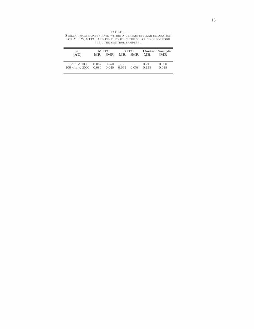
Following the same method describedin Wang et al. (2015), we calculate the stellarmultiplicity rate for MTPS as a function of a,i.e., companion semi-major axis. We find that for1 AU < a < 2000 AU, the stellar multiplicity ratefor MTPS is 13.3 ± 5.7%, which is significantly(3.2σ) lower than 33.6 ± 2.8% for the controlsample, i.e., the field stars in the solar neigh-borhood (Raghavan et al. 2010). We choose anupper limit of 2000 AU for comparison becausethe separation roughly corresponds to the smallestfield of view of co-added AO images, which havethe best sensitivity for stellar companion search.We further divide the semi-major axis of a stellarcompanion into two ranges, 1 AU < a < 100 AUand 100 AU < a < 2000 AU. We choose 100 AUbecause of two reasons. First, the separation isroughly the effective range of the perturbation ofcoplanarity by a companion star (see discussion of§5.2). Second, 100 AU is roughly the borderlineof RV and AO sensitivity (Wang et al. 2014b,a).Beyond 100 AU, the AO sensitivity is much higherthan that for the RV technique. The stellar multi-plicity rates for MTPS are 5.2±5.0% and 8.0±4.0%for 1 AU < a < 100 AU and 100 AU < a < 2000AU, respectively. In comparison, the stellar mul-tiplicity rates are 21.1 ± 2.8% and 12.5 ± 2.8% forthe control sample in these two stellar separationranges. The stellar multiplicity rate of MTPS for1 AU < a < 100 AU is lower (2.8σ) than thatfor the control sample. For 100 AU < a < 2000AU, the stellar multiplicity rates are comparablebetween MTPS and the control sample. Fig. 3illustrates the comparison of the stellar multiplicityrates in these two separation ranges.

5. DISCUSSION AND SUMMARY

5.1. Interpretation of the Stellar Multiplicity ofMTPS

The stellar multiplicity rate for MTPS (5.2 ±5.0%) is 2.8σ lower than that for stars in the so-lar neighborhood (21.1 ± 2.8%) for 1 AU < a <

100 AU. The difference may result from two possi-ble origins that are not mutually exclusive. First,

MTPS occur less frequently in multiple stellar sys-tems. Suppressive planet formation in multiplestellar systems has been noted in previous obser-vational works on both RV and transiting planetsamples (e.g., Eggenberger et al. 2011; Roell et al.2012; Wang et al. 2014b) and recently a theo-retical work (Touma & Sridhar 2015). However,other works suggest that the influence of a stellarcompanion may not be significant (Gilliland et al.2015; Horch et al. 2014) or may be facilitative de-pending on the stellar separation and planetarymass (Wang et al. 2015; Ngo et al. 2015).If suppressive planet formation does not play a

role, there may be another origin for the low stel-lar multiplicity rate: MTPS are less likely to beobserved in multiple stellar systems (Wang et al.2014b). Coplanarity of MTPS can be affected by anadditional stellar component. Thus the likelihood ofobserving multiple transiting planets is reduced.If suppressive planet formation plays a major role,

then our measurements of stellar multiplicity ratesindicate that within 100 AU, MTPS occur less fre-quently due to the influence of stellar companions.For 100 AU < a < 2000 AU, since the stellar mul-tiplicity rates are comparable (0.9σ difference) be-tween MTPS (8.0 ± 4.0%) and the control sample(12.5±2.8%), we conclude that the influence of stel-lar companions, if any, is too small to be observed.

5.2. Comparison to STPS

If coplanarity is responsible for the observed lowstellar multiplicity rate for MTPS, then we shouldexpect a difference of stellar multiplicity rate be-tween MTPS and STPS. Note that the influence ofstellar companions on coplanarity depends on stel-lar separations. If stellar separations are beyond∼100 AU, their influence on coplanarity is negli-gible (Wang et al. 2014b,a). Therefore, any differ-ence of stellar multiplicity rate beyond 100 AU ismore likely to be due to the origin of planet for-mation rather than the companions’ influence oncoplanarity.In 5.1, we show that beyond 100 AU the

stellar multiplicity rates are comparable betweenMTPS and the control sample. Here, we compareMTPS to STPS. Since these two populations likelyhave different dynamical history (Xie et al. 2014;Morton & Winn 2014), the comparison allows usto study whether the difference is related to stel-lar multiplicity.From CFOP, we select 89 Kepler STPS. The se-

lection criteria are the same as described in §2 withtwo exceptions: 1, the number of transiting planetis equal to one; 2, they must have AO images. Thestellar properties of these STPS are given in Ta-ble 3. The sample of these STPS is a subsampleof Kepler stars with high-resolution imaging obser-vations from CFOP (Ciardi 2015). Out of these89 Kepler stars, only 6 have RV observations. Sincethe RV technique is sensitive to close-in stellar com-panions, obtaining the statistics for stellar compan-ions within 100 AU is difficult. Therefore, we fo-cus on 100 AU < a < 2000 AU. The AO detec-tions are listed in Table 4. Following the same

5

method in Wang et al. (2015), we find that the stel-lar multiplicity rate is 6.4 ± 5.8% for STPS for100 AU < a < 2000 AU,. The value is consistentwith that for MTPS, i.e., 8.0± 4.0%. Therefore, wefind no evidence that stellar companions between100 and 2000 AU are responsible for the differenceof orbital configuration between MTPS and STPS.However, the difference may be caused by stellarcompanions within 100 AU, for which we do nothave adequate observational constraints.

5.3. Comparison to Previous Result

The same sample of 138 MTPS were studiedin Wang et al. (2014b). They found evidence of sup-pressive planet formation in tight binary stellar sys-tems with a < 20 AU. This finding is consistent withthe finding in this paper that the stellar multiplic-ity rate for MTPS is lower than the control samplewithin 100 AU at 2.8σ level. However, we cannotrule out another possibility that may cause the lowstellar multiplicity, i.e., the influence of stellar com-panions on coplanarity of planetary orbits.Combining newly obtained AO imaging data with

archival RV data, we improve the statistics of stellarcompanions of planet host stars at large semi-majoraxes. For example, in Wang et al. (2014b), stel-lar multiplicity rate can only be constrained within∼100 AU because of a lack of AO imaging data. Inthis work, we extend the constraints to 2000 AU.Even within 100 AU, the stellar companion statis-tics is improved by the AO imaging data. This isbecause the AO imaging technique complements theRV technique at semi-major axes at which the dy-namical signals are difficult to detect. The combi-nation of AO and RV data enables the detection ofa deficit of stellar companions to MTPS within 100AU.Wang et al. (2014a) combined RV and AO data

for 56 Kepler planet host stars. The stellar multi-plicity rate for a < 2000 AU was 43.2±5.7%, whichis a factor of three higher than what we reportedin this paper, i.e., 13.3 ± 5.7%. The discrepancyis due to two reasons. First, we exclude opticaldoubles whereas Wang et al. (2014a) included bothoptical doubles and physically associated compan-ions. A physical separation of 2000 AU roughly cor-responds to 3′′-6′′ angular separation (for the typ-ical distances to these Kepler stars), at which thephysical association probability is ∼50%. There-fore, roughly half of visual companions are expectedto be optical doubles around 2000 AU. Second, weconsidered statistics of stellar companions to planethost stars when calculating the incompleteness ofcompanion search (Wang et al. 2015). In compar-ison, Wang et al. (2014a) considered statistics ofstellar companions for stars in the solar neighbor-hood. The companion search incompleteness wasoverestimated in Wang et al. (2014a) because thestellar multiplicity rate for planet host stars is gen-erally lower than that for stars in the solar neighbor-hood especially for small semi-major axes. There-fore, the correction factor due to search incomplete-ness is smaller, resulting a lower stellar multiplicityrate.

5.4. Summary and Conclusion

We study the influence of stellar companions onMTPS using a sample of 138 Kepler MTPS. Wesearch for stellar companions to these planet hoststars with AO images and archival RV data. Intotal, we detected 42 stellar companions within 5′′

around 35 multi-planet host stars. The propertiesof detected stellar companions are summarized inTable 2. We also provide detection limits for allstars in our sample in Table 1.We compare the stellar multiplicity rate between

MTPS and a control sample, i.e., stars in the solarneighborhood. For semi-major axes 1 AU < a <

2000 AU the stellar multiplicity rate is 13.3± 5.7%for MTPS, which is 3.2σ lower than 33.6 ± 2.8%for the control sample, i.e., the field stars in thesolar neighborhood (Raghavan et al. 2010). Thedeficit of stellar companions to MTPS can be aresult of two origins, a suppressive planet forma-tion and the disruption of coplanarity due to stel-lar companions. Since the latter may only be ef-fective within 100 AU, we divide the semi-majoraxes into two ranges, 1 AU < a < 100 AU and100 AU < a < 2000 AU. The stellar multiplicityrate of MTPS for 1 AU < a < 100 AU is lower(2.8σ) than that for the control sample. The stellarmultiplicity rates are comparable between MTPSand the control sample for 100 AU < a < 2000 AU.We also compare the stellar multiplicity rates

for MTPS and STPS. No quantitative difference isfound between MTPS and STPS for 100 AU < a <

2000 AU. For 1 AU < a < 100 AU, our data are in-sufficient for comparative study between MTPS andSTPS because of a lack of RV data for STPS. Basedon these results, we cannot distinguish the two ori-gins that could be responsible for the low stellarmultiplicity rate for MTPS for 1 AU < a < 100AU. Future AO and RV follow-up observations fora larger sample are needed for such a comparativestudy between MTPS and STPS.Acknowledgements The authors thank the anony-mous referee for constructive comments and sug-gestions that greatly improve the paper. We wouldlike to thank the telescope operators and support-ing astronomers at the Palomar Observatory andthe Keck Observatory. Some of the data presentedherein were obtained at the W.M. Keck Observa-tory, which is operated as a scientific partnershipamong the California Institute of Technology, theUniversity of California and the National Aeronau-tics and Space Administration. The Observatorywas made possible by the generous financial sup-port of the W.M. Keck Foundation. The researchis made possible by the data from the Kepler Com-munity Follow-up Observing Program (CFOP). Theauthors acknowledge all the CFOP users who up-loaded the AO and RV data used in the paper.This research has made use of the NASA ExoplanetArchive, which is operated by the California Insti-tute of Technology, under contract with the Na-tional Aeronautics and Space Administration un-der the Exoplanet Exploration Program. J.W.X.acknowledges support from the National Natural

6 Wang

Science Foundation of China (Grant No. 11333002and 11403012), the Key Development Program ofBasic Research of China (973 program, Grant No.2013CB834900) and the Foundation for the Au-

thor of National Excellent Doctoral Dissertation(FANEDD) of PR China. J.W. acknowledges thetravel fund from the Key Laboratory of Modern As-tronomy and Astrophysics (Nanjing University).

REFERENCES

Adams, E. R., Ciardi, D. R., Dupree, A. K., Gautier, III,T. N., Kulesa, C., & McCarthy, D. 2012, AJ, 144, 42

Brandl, B., Hayward, T. L., Houck, J. R., Gull, G. E.,Pirger, B., & Schoenwald, J. 1997, in Society ofPhoto-Optical Instrumentation Engineers (SPIE)Conference Series, Vol. 3126, Adaptive Optics andApplications, ed. R. K. Tyson & R. Q. Fugate, 515

Burke, C. J., et al. 2014, ApJS, 210, 19Burruss, R. S., et al. 2014, in Presented at the Society of

Photo-Optical Instrumentation Engineers (SPIE)Conference, Vol. 9148, Society of Photo-OpticalInstrumentation Engineers (SPIE) Conference Series

Campante, T. L., et al. 2015, ApJ, 799, 170Ciardi, D. 2015, In Prep.Davies, R., & Kasper, M. 2012, ARA&A, 50, 305Duquennoy, A., & Mayor, M. 1991, A&A, 248, 485Eggenberger, A., Udry, S., Chauvin, G., Forveille, T.,

Beuzit, J.-L., Lagrange, A.-M., & Mayor, M. 2011, inIAU Symposium, Vol. 276, IAU Symposium, ed.A. Sozzetti, M. G. Lattanzi, & A. P. Boss, 409–410

Giguere, M. J., et al. 2012, ApJ, 744, 4Gilliland, R. L., Cartier, K. M. S., Adams, E. R., Ciardi,

D. R., Kalas, P., & Wright, J. T. 2015, AJ, 149, 24Han, E., Wang, S. X., Wright, J. T., Feng, Y. K., Zhao, M.,

Fakhouri, O., Brown, J. I., & Hancock, C. 2014, PASP,126, 827

Hayward, T. L., Brandl, B., Pirger, B., Blacken, C., Gull,G. E., Schoenwald, J., & Houck, J. R. 2001, PASP, 113,105

Horch, E. P., Howell, S. B., Everett, M. E., & Ciardi, D. R.2012, AJ, 144, 165

—. 2014, ApJ, 795, 60Huber, D., et al. 2014, ApJS, 211, 2Juric, M., & Tremaine, S. 2008, ApJ, 686, 603Kane, S. R., Ciardi, D. R., Gelino, D. M., & von Braun, K.

2012, MNRAS, 425, 757

Latham, D. W., et al. 2011, ApJ, 732, L24Law, N. M., et al. 2014, ApJ, 791, 35Lillo-Box, J., Barrado, D., & Bouy, H. 2012, A&A, 546, A10—. 2014, A&A, 566, A103Lissauer, J. J., et al. 2011, ApJS, 197, 8—. 2012, ApJ, 750, 112—. 2014, ApJ, 784, 44Morton, T. D., & Winn, J. N. 2014, ApJ, 796, 47Ngo, H., et al. 2015, ApJ, 800, 138Raghavan, D., et al. 2010, ApJS, 190, 1Roell, T., Neuhauser, R., Seifahrt, A., & Mugrauer, M.

2012, A&A, 542, A92Rowe, J. F., et al. 2014, ApJ, 784, 45Touma, J. R., & Sridhar, S. 2015, Nature, 524, 439Tremaine, S., & Dong, S. 2012, AJ, 143, 94Wang, J., Fischer, D. A., Horch, E. P., & Xie, J.-W. 2015,

ApJ, 806, 248Wang, J., Fischer, D. A., Xie, J.-W., & Ciardi, D. R. 2014a,

ApJ, 791, 111Wang, J., Xie, J.-W., Barclay, T., & Fischer, D. A. 2014b,

ApJ, 783, 4Winn, J. N., & Fabrycky, D. C. 2015, ARA&A, 53, 409Wizinowich, P. L., Acton, D. S., Lai, O., Gathright, J.,

Lupton, W., & Stomski, P. J. 2000, in Society ofPhoto-Optical Instrumentation Engineers (SPIE)Conference Series, Vol. 4007, Society of Photo-OpticalInstrumentation Engineers (SPIE) Conference Series, ed.P. L. Wizinowich, 2–13

Wright, J. T., et al. 2011, PASP, 123, 412Xie, J.-W. 2015, In Prep.Xie, J.-W., Wu, Y., & Lithwick, Y. 2014, ApJ, 789, 165

7

K00119 K00298 K00353

K01151 K01929 K1932

K2059 K2289 K4021

Fig. 1.— AO images for 9 KOIs with newly detected stellar companions within 2′′. All images cover a 2′′ by 2′′ sky regioncentering at the primary star. North is up and east is to the left. Linear color scale is chosen such that the central star (red)is normalized to 1 and the background (blue) represents 1/100 of the central star flux. Both central stars and detected stellarcompanions are marked by green circles. Photometric and astrometric information of detected stellar companions can be foundin Table 2.

8 Wang

1 2 3 4 5

Sep [arcsec]

0

2

4

6

8

10

∆M

ag

K03864 Palomar

0.5 1.0 1.5 2.0

Sep [arcsec]

0

2

4

6

8

10

K01241 Keck

Fig. 2.— Simulation for AO search completeness in comparison with contrast curve. Left panel shows an example for aPalomar AO image and right panel for a Keck AO image. Blue dots are artificial PSF injections at random separations,differential magnitudes and position angles that are successfully recovered by our detection pipeline. Red dots are injectionsthat are missed. AO contrast curves (§3.1) are plotted as black solid lines which generally trace the border line between blueand red dots.

Fig. 3.— Stellar multiplicity rate for multiple transiting planet systems (MTPS, green), single transiting planet systems(STPS, red), and the field stars in the solar neighborhood, i.e., the control sample in blue. The stellar multiplicity rates fordifferent samples are given in Table 5.

9

TABLE 1AO Sensitivity

Kepler Observation Limiting Delta Magnitude∗∗

KIC KOI Kmag i J H K Comp. Iso. Instrument Flt 0.1 0.2 0.5 1.0 2.0 4.0[mag] [mag] [mag] [mag] [mag] < 5′′ Prob.∗ [′′] [′′] [′′] [′′] [′′] [′′]

8554498 00005 11.665 11.485 10.542 10.257 10.213 yes · · · NIRC2 K 2.0 4.0 6.4 7.4 7.5 7.58554498 00005 11.665 11.485 10.542 10.257 10.213 yes · · · PHARO J 0.1 1.3 2.7 4.8 6.7 7.66521045 00041 11.197 11.030 10.081 9.804 9.768 no 0.96 ARIES K 0.1 1.2 3.4 5.9 7.2 7.56521045 00041 11.197 11.030 10.081 9.804 9.768 no 0.96 NIRC2 K 3.2 4.6 5.3 5.4 5.4 5.46521045 00041 11.197 11.030 10.081 9.804 9.768 no 0.96 PHARO J 0.4 3.6 4.5 6.6 7.6 7.76850504 00070 12.498 12.284 11.252 10.910 10.871 yes · · · PHARO J 0.4 3.0 4.5 6.4 7.3 7.411904151 00072 10.961 10.778 9.889 9.563 9.496 no 0.99 ARIES K 0.8 2.3 5.1 7.0 7.6 7.611904151 00072 10.961 10.778 9.889 9.563 9.496 no 0.99 PHARO J 0.5 3.3 4.3 6.5 7.9 8.110187017 00082 11.492 11.150 9.984 9.446 9.351 no 0.92 ARIES K 0.5 1.9 4.7 7.0 7.8 7.910187017 00082 11.492 11.150 9.984 9.446 9.351 no 0.92 NIRC2 K 2.6 4.5 5.4 5.6 5.6 5.65866724 00085 11.018 10.882 10.066 9.852 9.806 no 0.88 ARIES K 0.9 2.4 5.1 7.1 7.6 7.76462863 00094 12.205 12.057 11.218 10.957 10.926 no 0.75 ARIES K 0.1 0.9 4.2 6.8 7.4 7.38456679 00102 12.566 12.384 11.398 11.124 11.055 yes · · · NIRC2 K 2.2 4.3 6.3 7.2 7.3 7.38456679 00102 12.566 12.384 11.398 11.124 11.055 yes · · · PHARO J 0.7 2.2 4.0 5.8 6.9 7.44914423 00108 12.287 12.132 11.193 10.941 10.873 yes · · · NIRC2 K 2.5 4.0 5.7 6.1 6.2 6.24914423 00108 12.287 12.132 11.193 10.941 10.873 yes · · · PHARO J 0.8 3.2 4.4 6.5 7.6 7.76678383 00111 12.596 12.442 11.558 11.251 11.209 no 0.89 PHARO J 0.6 2.9 4.2 6.1 7.1 7.310984090 00112 12.772 12.602 11.698 11.402 11.367 no 0.84 PHARO J 0.5 2.4 3.9 6.1 8.0 8.510984090 00112 12.772 12.602 11.698 11.402 11.367 no 0.84 PHARO K 0.0 1.8 4.8 5.4 6.9 7.19579641 00115 12.791 12.654 11.811 11.555 11.503 yes · · · ARIES K 0.2 1.8 4.9 6.6 6.8 6.88395660 00116 12.882 12.706 11.752 11.494 11.431 no 0.91 ARIES K 0.4 1.9 4.9 7.0 7.3 7.28395660 00116 12.882 12.706 11.752 11.494 11.431 no 0.91 NIRC2 K 2.9 4.5 6.2 6.5 6.6 6.610875245 00117 12.487 12.309 11.392 11.114 11.060 no 0.74 PHARO J 0.1 0.7 2.1 3.7 5.9 7.910875245 00117 12.487 12.309 11.392 11.114 11.060 no 0.74 PHARO K 0.4 1.5 3.6 5.0 6.8 7.29471974 00119 12.654 12.452 11.430 11.065 10.983 yes · · · PHARO J 0.0 0.6 1.8 3.3 4.5 7.39471974 00119 12.654 12.452 11.430 11.065 10.983 yes · · · PHARO K 0.0 0.7 2.7 4.3 5.5 6.55094751 00123 12.365 12.206 11.314 11.046 11.001 no 0.86 NIRC2 K 2.4 4.3 6.0 6.5 6.5 6.55094751 00123 12.365 12.206 11.314 11.046 11.001 no 0.86 PHARO J 0.0 1.2 3.3 5.3 7.0 7.65735762 00148 13.040 12.761 11.702 11.292 11.221 yes · · · NIRC2 K 2.3 4.2 5.7 6.3 6.3 6.35735762 00148 13.040 12.761 11.702 11.292 11.221 yes · · · PHARO J 0.2 2.8 4.0 6.1 7.4 7.612252424 00153 13.461 13.097 11.886 11.360 11.255 no 0.93 ARIES K 0.0 1.0 4.1 6.4 6.7 6.712252424 00153 13.461 13.097 11.886 11.360 11.255 no 0.93 NIRC2 K 2.0 4.2 4.9 4.9 4.9 4.912252424 00153 13.461 13.097 11.886 11.360 11.255 no 0.93 PHARO J 0.1 0.9 2.2 3.9 6.1 7.612252424 00153 13.461 13.097 11.886 11.360 11.255 no 0.93 PHARO K 0.5 1.7 3.7 5.0 6.6 6.811512246 00168 13.438 13.244 12.353 12.047 11.998 no 0.69 PHARO K 0.4 1.4 3.3 4.8 5.5 5.64349452 00244 10.734 9.764 9.532 9.493 no 0.91 NIRC2 K 2.8 4.4 5.3 5.4 5.4 5.44349452 00244 10.734 9.764 9.532 9.493 no 0.91 PHARO J 0.6 2.7 3.9 5.8 7.9 8.54349452 00244 10.734 9.764 9.532 9.493 no 0.91 PHARO K 0.8 2.7 5.0 5.6 7.7 8.18478994 00245 9.705 8.356 8.000 7.942 no 0.95 ARIES K 0.5 1.8 4.8 7.3 8.2 8.48478994 00245 9.705 8.356 8.000 7.942 no 0.95 NIRC2 K 2.4 4.1 6.1 6.7 6.9 6.98478994 00245 9.705 8.356 8.000 7.942 no 0.95 PHARO K 1.0 2.3 5.0 6.7 8.6 9.911295426 00246 9.997 9.820 8.975 8.662 8.588 no 0.97 ARIES K 0.6 2.0 4.4 6.8 7.7 7.811295426 00246 9.997 9.820 8.975 8.662 8.588 no 0.97 NIRC2 K 2.9 4.4 6.0 6.3 6.4 6.48292840 00260 10.500 9.616 9.407 9.344 no 0.92 ARIES K 0.1 1.5 3.7 6.2 7.7 8.211807274 00262 10.421 10.313 9.518 9.250 9.197 no 0.89 ARIES K 0.7 2.5 4.8 6.8 7.3 7.56528464 00270 11.411 10.088 9.770 9.701 no 0.80 ARIES K 0.2 1.7 4.0 6.1 7.0 7.19451706 00271 11.485 11.358 10.536 10.300 10.234 no 0.90 ARIES K 0.7 2.3 4.6 6.8 7.2 7.49451706 00271 11.485 11.358 10.536 10.300 10.234 no 0.90 NIRC2 K 2.7 4.5 6.6 7.4 7.5 7.59451706 00271 11.485 11.358 10.536 10.300 10.234 no 0.90 PHARO J 0.7 2.4 4.5 5.5 7.5 7.89451706 00271 11.485 11.358 10.536 10.300 10.234 no 0.90 PHARO K 0.0 0.9 2.4 4.1 5.4 5.88077137 00274 11.390 11.258 10.373 10.094 10.109 no 0.88 ARIES K 0.7 2.4 5.2 7.1 7.6 7.710586004 00275 11.696 10.600 10.325 10.252 no 0.86 PHARO J 1.2 2.7 5.2 5.9 7.5 7.710586004 00275 11.696 10.600 10.325 10.252 no 0.86 PHARO K 0.5 2.5 3.7 5.9 8.0 8.712314973 00279 11.684 11.563 10.708 10.472 10.429 yes · · · NIRC2 K 2.1 4.3 5.5 5.6 5.7 5.75088536 00282 11.529 10.810 10.529 10.490 yes · · · NIRC2 K 2.4 4.3 6.6 7.4 7.5 7.55088536 00282 11.529 10.810 10.529 10.490 yes · · · PHARO K 0.5 1.5 3.6 5.7 7.3 7.65695396 00283 11.525 11.334 10.418 10.127 10.079 no 0.95 NIRC2 K 2.5 3.9 5.2 5.5 5.5 5.55695396 00283 11.525 11.334 10.418 10.127 10.079 no 0.95 PHARO J 0.0 0.5 1.7 3.1 5.2 7.45695396 00283 11.525 11.334 10.418 10.127 10.079 no 0.95 PHARO K 0.8 2.2 4.1 5.8 7.3 7.76021275 00284 11.818 11.666 10.797 10.516 10.424 yes · · · PHARO J 0.0 0.2 1.7 3.2 4.6 5.86021275 00284 11.818 11.666 10.797 10.516 10.424 yes · · · PHARO K 0.0 0.4 1.6 3.7 5.1 7.96196457 00285 11.565 10.747 10.470 10.403 yes · · · PHARO J 0.0 0.7 2.1 3.9 5.9 7.06196457 00285 11.565 10.747 10.470 10.403 yes · · · PHARO K 0.4 1.9 3.9 5.6 7.1 7.510386922 00289 12.747 12.540 11.534 11.220 11.187 no 0.92 NIRC2 K 2.5 4.5 6.5 7.2 7.3 7.310386922 00289 12.747 12.540 11.534 11.220 11.187 no 0.92 PHARO K 0.2 1.0 3.1 5.0 6.2 6.510933561 00291 12.848 12.642 11.680 11.399 11.320 no 0.69 PHARO K 0.3 1.0 3.0 4.5 5.0 5.111547513 00295 12.324 12.155 11.260 10.984 10.951 no 0.77 PHARO K 0.9 1.8 3.6 5.7 6.7 6.912785320 00298 12.713 12.355 11.295 10.946 10.885 yes · · · PHARO J 0.0 0.5 1.9 3.3 5.0 5.812785320 00298 12.713 12.355 11.295 10.946 10.885 yes · · · PHARO K 0.5 1.2 3.1 4.5 4.9 5.83642289 00301 12.730 12.586 11.722 11.508 11.456 no 0.72 PHARO K 0.0 0.9 3.0 4.7 5.3 5.46029239 00304 12.549 12.377 11.472 11.192 11.109 no 0.83 PHARO K 0.7 1.7 4.2 5.6 6.5 6.76289257 00307 12.797 12.650 11.806 11.552 11.488 no 0.73 PHARO K 0.0 0.9 3.1 4.7 5.2 5.37050989 00312 12.459 10.804 10.573 10.519 yes · · · NIRC2 K 1.4 3.3 5.4 6.0 6.1 6.07050989 00312 12.459 10.804 10.573 10.519 yes · · · PHARO K 0.2 1.3 3.2 5.5 7.1 7.77419318 00313 12.990 12.736 11.650 11.229 11.165 no 0.81 PHARO J 0.4 1.3 2.8 4.8 7.1 8.17419318 00313 12.990 12.736 11.650 11.229 11.165 no 0.81 PHARO K 0.5 1.8 3.7 5.3 6.9 7.17603200 00314 12.925 12.457 10.293 9.680 9.506 no 0.91 PHARO K 0.3 1.1 3.0 4.9 6.3 6.68008067 00316 12.701 12.494 11.530 11.222 11.167 no 0.82 PHARO J 0.0 0.5 1.6 3.2 5.4 6.98008067 00316 12.701 12.494 11.530 11.222 11.167 no 0.82 PHARO K 0.3 1.4 3.2 4.9 6.1 6.48753657 00321 12.520 12.312 11.340 11.035 10.970 no 0.92 NIRC2 K 2.8 4.3 6.1 6.7 6.8 6.89880467 00326 12.960 12.960 14.774 13.236 13.085 yes · · · PHARO K 0.1 1.0 3.9 4.6 4.9 4.99881662 00327 12.996 12.858 11.989 11.759 11.709 no 0.91 PHARO K 0.1 0.9 2.7 4.2 4.6 4.710290666 00332 13.046 12.847 11.910 11.569 11.475 no 0.76 PHARO K 0.2 0.8 2.5 4.2 5.4 5.610552611 00338 13.448 13.116 11.955 11.485 11.393 no 0.68 PHARO K 0.5 1.5 3.6 5.3 6.3 6.310878263 00341 13.338 13.106 12.087 11.750 11.698 no 0.71 ARIES K 0.0 0.5 2.4 4.9 6.0 6.110982872 00343 13.203 13.013 12.092 11.801 11.762 no 0.73 PHARO K 0.3 1.1 2.7 4.5 5.4 5.511566064 00353 13.374 13.251 12.455 12.263 12.228 yes · · · PHARO K 0.1 0.9 2.4 3.6 4.6 4.811568987 00354 13.235 13.057 12.063 11.775 11.708 yes · · · PHARO K 0.2 0.9 2.6 4.4 5.4 5.57175184 00369 11.992 11.868 11.050 10.830 10.792 no 0.76 PHARO K 0.2 1.0 3.0 4.9 5.8 6.112068975 00623 11.811 11.685 10.814 10.577 10.535 no 0.85 NIRC2 K 2.0 4.1 6.0 6.4 6.5 6.54478168 00626 13.490 13.339 12.514 12.195 12.205 yes · · · PHARO K 0.8 1.8 4.5 5.5 5.8 6.04563268 00627 13.307 13.119 12.203 11.938 11.905 no 0.69 PHARO K 0.0 0.3 2.1 4.1 5.9 7.05966154 00655 13.004 12.872 12.037 11.784 11.737 no 0.75 PHARO K 0.0 1.0 2.4 4.3 5.1 5.26685609 00665 13.182 13.005 12.100 11.841 11.805 no 0.71 PHARO K 0.3 1.3 2.9 4.5 5.4 5.57509886 00678 13.283 12.997 11.927 11.488 11.447 no 0.75 PHARO K 0.1 1.0 2.8 4.5 5.5 5.77515212 00679 13.178 13.038 11.931 11.699 11.620 no 0.74 PHARO K 0.4 1.3 3.0 4.7 5.7 5.99590976 00710 13.294 13.128 12.319 12.176 12.103 no 0.68 PHARO K 0.0 1.0 2.6 4.2 5.0 5.19873254 00717 13.387 13.182 12.194 11.868 11.793 no 0.72 PHARO K 0.2 1.3 3.2 4.7 5.6 5.89950612 00719 13.177 12.899 11.206 10.672 10.550 no 0.94 NIRC2 K 2.7 4.5 6.6 7.8 8.0 8.011013201 00972 9.275 9.392 8.816 8.765 8.736 no 0.86 PHARO K 1.3 2.5 5.1 6.8 8.8 9.31871056 01001 13.038 12.851 11.918 11.692 11.591 yes · · · PHARO K 0.2 1.0 2.7 4.4 5.4 5.68280511 01151 13.404 13.198 12.198 11.819 11.745 yes · · · PHARO K 0.3 1.3 3.1 4.6 5.7 5.810350571 01175 13.290 13.075 12.061 11.704 11.617 no 0.67 PHARO K 0.0 0.8 2.4 4.1 5.2 5.43939150 01215 13.420 13.226 12.288 12.003 11.966 no 0.68 PHARO K 0.5 1.4 3.5 5.1 5.7 5.86448890 01241 12.440 12.090 10.813 10.330 10.227 no 0.81 NIRC2 K 2.1 3.6 5.4 6.0 6.1 6.06448890 01241 12.440 12.090 10.813 10.330 10.227 no 0.81 PHARO K 0.1 0.9 2.8 5.0 6.8 7.510794087 01316 11.926 11.694 10.894 10.606 10.562 yes · · · ARIES K 0.4 1.6 3.5 5.8 7.9 8.210794087 01316 11.926 11.694 10.894 10.606 10.562 yes · · · NIRC2 K 2.4 4.4 6.9 7.6 7.7 7.711336883 01445 12.320 12.209 11.406 11.171 11.151 no 0.86 PHARO K 0.2 1.0 2.8 4.9 6.4 6.97869917 01525 12.082 12.009 11.250 11.065 11.039 no 0.71 PHARO K 0.4 1.1 3.0 4.9 6.5 7.14741126 01534 13.470 13.325 12.539 12.270 12.241 no 0.69 PHARO K 0.4 1.1 3.0 4.5 5.1 5.26268648 01613 11.049 10.588 10.316 10.282 yes · · · NIRC2 K 2.4 4.5 6.3 7.6 7.7 7.76268648 01613 11.049 10.588 10.316 10.282 yes · · · PHARO K 0.0 0.4 4.4 5.9 7.0 7.36975129 01628 12.949 12.775 11.902 11.664 11.596 no 0.83 PHARO K 0.2 1.0 2.9 4.5 4.9 5.06616218 01692 12.557 12.313 11.242 10.850 10.778 yes · · · PHARO K 0.2 1.0 4.1 5.3 6.4 6.89909735 01779 13.297 13.077 12.148 11.832 11.766 no 0.80 NIRC2 K 1.8 4.1 5.2 5.5 5.5 5.49909735 01779 13.297 13.077 12.148 11.832 11.766 no 0.80 PHARO K 0.1 1.0 2.7 4.5 5.5 5.611551692 01781 12.231 11.884 10.641 10.161 10.062 yes · · · NIRC2 J 1.7 2.6 4.2 5.5 5.8 5.611551692 01781 12.231 11.884 10.641 10.161 10.062 yes · · · NIRC2 K 1.5 3.3 5.1 5.8 5.9 5.811551692 01781 12.231 11.884 10.641 10.161 10.062 yes · · · PHARO K 0.1 1.1 3.0 5.2 6.8 7.39529744 01806 13.474 13.337 12.546 12.283 12.307 yes · · · PHARO K 0.3 1.2 3.1 4.5 5.0 4.98240797 01809 12.706 12.474 11.621 11.300 11.249 no 0.73 PHARO K 0.2 1.0 3.1 5.3 6.1 6.22989404 01824 12.722 12.567 11.689 11.423 11.354 no 0.73 PHARO K 0.3 1.3 3.3 5.0 5.9 6.010130039 01909 12.776 12.612 11.710 11.448 11.409 no 0.73 PHARO K 0.3 1.2 3.2 4.8 5.6 5.710136549 01929 12.727 12.530 11.537 11.257 11.183 yes · · · PHARO K 0.3 1.1 3.2 4.9 5.7 5.85511081 01930 12.119 11.957 11.098 10.841 10.756 no 0.85 NIRC2 K 2.6 4.6 6.7 7.3 7.4 7.45202905 01932 12.345 12.366 11.725 11.629 11.583 yes · · · NIRC2 H 1.4 2.8 4.4 5.1 5.3 5.35202905 01932 12.345 12.366 11.725 11.629 11.583 yes · · · NIRC2 J 1.3 2.4 3.9 5.0 5.3 5.25202905 01932 12.345 12.366 11.725 11.629 11.583 yes · · · NIRC2 K 1.5 3.8 4.9 5.4 5.4 5.35202905 01932 12.345 12.366 11.725 11.629 11.583 yes · · · PHARO K 0.2 1.1 3.1 5.3 6.6 6.89892816 01955 13.147 13.025 12.220 11.999 11.957 no 0.76 PHARO K 0.3 1.1 3.0 4.6 5.3 5.412154526 02004 13.351 13.150 12.174 11.872 11.803 no 0.78 PHARO K 0.4 1.2 2.8 4.5 5.5 5.75384079 02011 12.556 12.419 11.708 11.454 11.377 yes · · · PHARO K 0.1 0.9 2.7 4.8 6.2 6.59489524 02029 12.957 12.694 11.610 11.178 11.132 no 0.91 NIRC2 K 2.2 4.4 6.4 7.3 7.3 7.32307415 02053 12.992 12.839 12.000 11.745 11.704 no 0.71 PHARO K 0.1 0.8 2.5 4.2 4.7 4.712301181 02059 12.906 12.558 11.305 10.791 10.664 yes · · · NIRC2 K 2.4 4.0 5.6 7.4 7.8 7.812301181 02059 12.906 12.558 11.305 10.791 10.664 yes · · · PHARO K 0.0 0.0 1.7 3.6 4.8 4.96021193 02148 13.353 13.112 12.111 11.755 11.697 no 0.68 PHARO K 0.5 1.5 3.6 5.2 6.0 6.29006186 02169 12.404 12.172 11.137 10.735 10.662 yes · · · PHARO K 0.2 1.1 2.9 5.0 6.8 7.111774991 02173 12.879 12.522 11.243 10.752 10.674 no 0.94 NIRC2 K 2.8 4.6 6.6 7.3 7.5 7.49022166 02175 12.848 12.626 11.600 11.229 11.175 no 0.85 NIRC2 K 2.9 4.6 6.5 7.1 7.2 7.23867615 02289 13.358 13.193 12.341 12.092 12.005 yes · · · PHARO K 0.3 1.3 3.1 4.6 5.6 5.78013439 02352 10.421 9.721 9.547 9.504 no 0.92 NIRC2 K 2.5 4.6 6.8 7.5 7.5 7.58013439 02352 10.421 9.721 9.547 9.504 no 0.92 PHARO K 1.1 2.7 5.0 6.8 7.8 8.112306058 02541 13.007 12.717 11.564 11.072 10.970 no 0.66 PHARO K 0.2 0.9 2.7 4.6 5.8 6.18883329 02595 13.223 13.107 12.325 12.087 11.995 no 0.68 PHARO K 0.2 1.0 2.6 4.4 5.5 5.711253827 02672 11.921 11.703 10.672 10.356 10.285 yes · · · PHARO K 0.2 1.4 4.0 5.9 6.8 6.88022489 02674 13.349 13.159 12.169 11.859 11.825 no 0.81 PHARO K 0.5 1.5 3.1 4.8 5.6 5.77202957 02687 10.158 9.973 9.052 8.761 8.693 no 0.88 PHARO K 0.9 2.9 5.6 7.5 8.8 8.911071200 02696 12.998 12.901 12.188 12.032 11.950 no 0.66 PHARO K 0.0 0.7 2.2 4.0 4.7 4.812206313 02714 13.312 13.160 12.277 12.065 11.987 no 0.71 PHARO K 0.3 1.3 3.1 4.7 5.4 5.56026737 02949 13.313 13.135 12.222 11.973 11.903 yes · · · PHARO K 0.5 1.6 3.4 5.2 5.8 5.96278762 03158 8.717 7.244 6.772 6.703 yes · · · NIRC2 K 2.7 4.6 5.8 6.1 6.1 6.16278762 03158 8.717 7.244 6.772 6.703 yes · · · PHARO J 0.0 1.6 3.5 5.3 7.1 8.96278762 03158 8.717 7.244 6.772 6.703 yes · · · PHARO K 1.5 3.4 5.8 7.4 8.9 9.79002538 03196 11.525 11.405 10.547 10.335 10.276 no 0.90 NIRC2 K 2.6 4.4 6.6 7.5 7.6 7.69002538 03196 11.525 11.405 10.547 10.335 10.276 no 0.90 PHARO K 0.3 1.3 3.9 5.5 6.6 7.08644365 03384 13.204 13.008 12.022 11.757 11.724 no 0.72 PHARO K 0.4 1.4 3.1 4.8 5.7 5.83561464 03398 13.489 13.361 12.556 12.311 12.289 no 0.80 PHARO K 0.9 2.4 4.9 5.5 5.9 5.911754430 03403 13.102 12.921 12.012 11.694 11.638 no 0.79 PHARO K 0.2 1.1 2.9 4.7 5.6 5.79117416 03425 13.266 12.957 11.897 11.610 11.514 no 0.84 NIRC2 K 2.3 4.3 6.4 7.2 7.3 7.36058816 03500 13.214 13.038 12.161 11.870 11.826 yes · · · PHARO K 0.3 1.1 2.9 4.4 5.2 5.42581316 03681 11.690 10.953 10.728 10.688 no 0.92 NIRC2 K 2.2 4.6 5.8 5.9 5.9 5.94164922 03864 12.914 12.604 11.489 11.013 10.915 no 0.77 PHARO K 0.1 1.0 2.9 4.7 5.5 5.611967788 04021 13.166 12.513 11.797 11.538 11.487 yes · · · PHARO K 0.0 0.4 1.8 2.9 4.0 4.47100673 04032 12.639 12.432 11.421 11.034 10.989 no 0.77 PHARO K 0.0 0.6 1.9 4.1 6.0 6.45688683 04097 13.435 12.965 11.614 10.958 10.841 no 0.85 PHARO K 0.3 1.4 3.3 5.1 6.2 6.58890924 04269 13.263 12.943 11.718 11.249 11.136 no 0.79 PHARO K 0.0 0.9 2.5 4.4 5.7 6.04548011 04288 12.400 12.246 11.331 11.106 11.025 yes · · · PHARO K 0.3 1.1 3.0 5.3 6.7 7.1

Note. — ∗: Isolation probability is the probability of a KOI being isolated within 2000 AU (i.e., has no stellar companion within 2000 AU) given the AO and/or RV data and/ordynamical analysis (see §3.3). For stars with detected nearby stellar companions, the physical association probability can be found in Table 2. ∗∗: Limiting Delta Magnitudesare 5-σ limit.

10 Wang

TABLE 2Visual companion detections with AO data for Kepler MTPS.

KOI Star# Telescope Filter ∆ Mag∗ Separation∗∗ Distance∗∗∗ PA Association∗∗∗∗ ref.†

Primary Secondary Probability(mag) (arcsec) (AU) (pc) (pc) (deg)

K00005 1 Keck K 2.20 0.14 40.12 286.671.1−15.8307.4 > 0.90 CFOP

K00070 1 Palomar J 4.41 3.77 1052.60 279.525.3−23.651.8 0.52 A12

K00102 1 Palomar J 1.12 2.84 934.31 329.475.0−30.5222.2 > 0.90 A12

K00108 1 Palomar J 5.71 2.51 891.07 354.645.4−39.2285.2 0.48 A12

K00108 2 Palomar J 5.60 3.23 1145.12 354.645.4−39.2100.8 0.30 A12

K00108 3 Palomar J 6.60 5.00 1773.09 354.645.4−39.2112.5 0.00 A12

K00115 1 MMT K 5.06 4.00 2168.27 542.1140.6−97.089.7 0.33 A12

K00119 1 Palomar J 0.16 1.05 327.89 313.0106.8−62.2380.8499.6−154.5

119.1 > 0.90 this workK00119 1 Palomar K 0.22 1.04 326.17 313.0106.8−62.2

380.8499.6−154.5120.2 > 0.90 this work

K00148 1 Palomar J 4.75 2.51 775.44 308.727.0−17.2245.6 0.78 A12

K00148 2 Palomar J 3.14 4.43 1368.74 308.727.0−17.2220.4 0.73 A12

K00279 1 Keck K 2.35 0.92 247.44 268.6187.6−46.3247.3 > 0.90 CFOP

K00282 1 Palomar K 3.86 4.16 1408.24 338.816.9−26.5210.3 0.84 CFOP

K00284 1 Palomar J 0.24 0.87 229.45 264.734.4−39.4339.5347.4−146.8

95.8 > 0.90 A12K00284 1 Palomar K 0.24 0.86 226.48 264.734.4−39.4

339.5347.4−146.896.7 > 0.90 A12

K00285 1 Palomar J 4.19 1.50 676.86 452.718.4−47.03855.92632.5−3163.9

137.7 > 0.90 CFOPK00285 1 Palomar K 4.08 1.50 677.09 452.718.4−47.0

3855.92632.5−3163.9137.7 > 0.90 CFOP

K00298 1 Palomar J 0.24 2.00 581.07 290.2300.0−54.4247.2335.0−68.1

272.8 > 0.90 this workK00298 1 Palomar K 0.08 1.96 570.05 290.2300.0−54.4

247.2335.0−68.1272.5 > 0.90 this work

K00312 1 Palomar K 6.67 3.01 950.62 316.133.3−25.9104.4 0.34 this work

K00312 2 Palomar K 5.84 4.97 1569.91 316.133.3−25.9121.7 0.33 this work

K00326 1 Palomar K 1.03 3.49 27865.11 7989.41953.2−1200.3269.4 0.89 this work

K00353 1 Palomar K 3.07 1.04 820.45 789.7151.9−103.223.0 > 0.90 this work

K00353 2 Palomar K 4.15 1.43 1131.97 789.7151.9−103.2236.3 > 0.90 this work

K00354 1 Palomar K 4.83 3.73 1425.50 382.129.8−25.5210.1 0.36 this work

K00626 1 Palomar K 5.30 2.75 1463.00 532.339.1−43.4167.9 0.21 this work

K01151 1 Palomar K 2.25 0.76 316.71 419.553.7−50.0306.6 > 0.90 this work

K01316 1 MMT K 5.81 2.78 1249.69 449.6185.2−96.34.8 0.68 CFOP (Dupree)

K01613 1 Keck K 1.00 0.22 79.49 364.321.7−19.1184.6 > 0.90 CFOP

K01613 1 Palomar K 1.16 0.21 75.31 364.321.7−19.1183.4 > 0.90 CFOP

K01692 1 Palomar K 6.36 3.17 841.66 265.414.6−19.8337.2 0.31 this work

K01781 1 Keck J 2.71 3.48 607.66 174.810.7−14.8508.7569.0−178.8

332.4 > 0.90 this workK01781 1 Keck K 2.35 3.47 606.92 174.810.7−14.8

508.7569.0−178.8332.2 > 0.90 this work

K01781 1 Palomar K 2.29 3.43 599.24 174.810.7−14.8508.7569.0−178.8

332.4 > 0.90 this work

K01806 1 Palomar K 1.45 3.43 2096.38 612.162.3−70.2249.7 0.90 this work

K01929 1 Palomar K 4.86 1.37 835.32 608.864.2−162.1163.0 > 0.90 this work

K01932 1 Keck J 4.08 0.54 1165.27 2171.2444.3−885.710489.32415.5−10378.5

116.6 > 0.90 this workK01932 1 Keck H 3.37 0.52 1129.01 2171.2444.3−885.7

10489.32415.5−10378.5115.3 > 0.90 this work

K01932 1 Keck K 3.12 0.52 1138.78 2171.2444.3−885.710489.32415.5−10378.5

115.1 > 0.90 this work

K01932 2 Palomar K 4.12 4.57 9928.21 2171.2444.3−885.7312.9 0.51 this work

K02011 1 Palomar K 2.73 4.95 2312.74 467.159.2−68.5292.1 0.82 this work

K02059 1 Keck K 0.14 0.39 92.93 238.413.8−15.7289.5 > 0.90 this work

K02059 1 Palomar K 0.14 0.38 91.43 238.413.8−15.7289.0 > 0.90 this work

K02169 1 Palomar K 2.74 3.49 1026.94 294.197.4−29.0289.0 > 0.90 this work

K02289 1 Palomar K 2.78 0.94 535.74 570.599.2−67.8221.2 > 0.90 this work

K02672 1 Palomar K 3.46 0.65 152.28 236.0126.7−46.5305.5 > 0.90 CFOP

K02672 2 Palomar K 6.04 4.62 1090.18 236.0126.7−46.5310.5 0.26 this work

K02949 1 Palomar K 3.86 2.35 1442.31 613.1598.6−111.5311.0 0.81 this work

K03158 1 Palomar J 2.39 1.83 54.30 29.61.4−3.178.853.8−64.7

253.3 > 0.90 C15K03158 1 Keck K 2.21 1.86 55.05 29.61.4−3.1

78.853.8−64.7252.8 > 0.90 C15

K03158 1 Palomar K 2.13 1.83 54.35 29.61.4−3.178.853.8−64.7

253.1 > 0.90 C15

K03500 1 Palomar K 3.35 2.53 1150.97 455.260.4−44.7140.0 0.90 this work

K04021 1 Palomar K 0.33 1.74 1886.56 1085.2303.3−221.0115.8 > 0.90 this work

K04288 1 Palomar K 6.59 2.93 1039.80 354.861.1−37.1279.8 0.03 this work

Note. — References: A12 - Adams et al. (2012); C15 - Campante et al. (2015). ∗: Typical ∆ Mag uncertainty is 0.1 mag. The uncertainty is estimated from the companion injection simulation

described in §3.3. ∗∗: Typical angular separation uncertainty is 0.05′′. The uncertainty is estimated from the companion injection simulation described in §3.3. ∗∗∗: Distance is estimated based onstellar properties of primary stars (Huber et al. 2014) and color information of secondary stars (see §4.1 in Wang et al. 2015, for more details). ∗∗∗∗: Association probability has 10% uncertainty

due to statistical error in simulation. †: AO images from CFOP are provided by David Ciardi unless otherwise noted.

11

TABLE 3Stellar Parameters For STPS

KOI KIC α δ Kp Teff log g [Fe/H](h:m:s) (d:m:s) (mag) (K) (cgs) (dex)

00042 8866102 18:52:36.17 45:08:23.4 9.36 6325 4.26 0.0100069 3544595 19:25:40.39 38:40:20.49 9.93 5669 4.47 -0.1800084 2571238 19:21:40.99 37:51:06.48 11.90 5543 4.57 -0.1400087 10593626 19:16:52.2 47:53:04.06 11.66 5642 4.44 -0.2700092 7941200 18:53:29.96 43:47:17.59 11.67 5952 4.49 -0.0400103 2444412 19:26:44 37:45:05.73 12.59 5653 4.55 -0.0600118 3531558 19:09:27.07 38:38:58.56 12.38 5747 4.18 0.0300122 8349582 18:57:55.79 44:23:52.95 12.35 5699 4.17 0.3000180 9573539 18:57:34.63 46:14:56.69 13.02 5691 4.54 -0.0600257 5514383 18:58:32.45 40:43:11.39 10.87 6184 4.36 0.1200261 5383248 19:48:16.71 40:31:30.47 10.30 5763 4.53 0.0400265 12024120 19:48:04.52 50:24:32.33 11.99 6036 4.32 0.0800268 3425851 19:02:54.91 38:30:25.1 10.56 6343 4.26 -0.0400269 7670943 19:09:22.98 43:22:42.21 10.93 6463 4.24 0.0900273 3102384 19:09:54.84 38:13:43.82 11.46 5739 4.40 0.3500276 11133306 19:18:39.46 48:42:22.36 11.85 5982 4.32 -0.0200280 4141376 19:06:45.47 39:12:42.88 11.07 6134 4.42 -0.2400281 4143755 19:10:37.2 39:14:39.44 11.95 5622 4.09 -0.4000292 11075737 19:09:18.39 48:40:24.35 12.87 5802 4.42 -0.2000299 2692377 19:02:38.8 37:57:52.2 12.90 5580 4.54 0.1800303 5966322 19:34:42.08 41:17:43.3 12.19 5598 4.32 -0.1200306 6071903 19:57:16.69 41:23:04.7 12.63 5377 4.58 0.1000344 11015108 18:53:21.67 48:32:56.55 13.40 5957 4.35 -0.0400364 7296438 19:43:29.36 42:52:52.14 10.09 5749 4.17 -0.2000374 8686097 19:22:30.06 44:52:26.25 12.21 5839 4.20 -0.2200974 9414417 19:43:12.64 45:59:17.08 9.58 6253 4.00 -0.1300975 3632418 19:09:26.84 38:42:50.46 8.22 6131 4.03 -0.1501162 10528068 19:15:28.37 47:45:33.95 12.78 6126 4.28 -0.2801311 10713616 18:54:07.91 48:05:39.34 13.50 6190 4.18 -0.1001442 11600889 19:04:08.72 49:36:52.24 12.52 5626 4.40 0.3401537 9872292 18:45:50.82 46:47:23.62 11.74 6260 4.05 0.1001612 10963065 18:59:08.69 48:25:23.62 8.77 6104 4.29 -0.2001615 4278221 19:41:17.4 39:22:35.37 11.52 5977 4.47 0.2101618 7215603 19:44:11.37 42:44:34.84 11.60 6173 4.19 0.1701619 4276716 19:39:57.66 39:20:46.96 11.76 4827 4.60 -0.3401808 7761918 19:38:58.4 43:27:40.35 12.49 6277 4.35 -0.0601883 11758544 19:16:56.01 49:56:20.15 11.89 6287 4.34 0.0201890 7449136 19:32:19.08 43:04:25.36 11.70 6099 4.13 0.0401925 9955598 19:34:43.01 46:51:09.94 9.44 5460 4.50 0.0801962 5513648 18:56:56.15 40:47:40.34 10.77 5904 4.13 -0.0701964 7887791 19:22:48.89 43:36:25.95 10.69 5547 4.39 -0.0602032 2985767 19:22:06.42 38:08:34.72 12.26 5568 4.50 -0.0402087 6922710 18:46:14.75 42:27:01.8 11.86 5930 4.40 0.0702110 11460462 19:37:52.45 49:19:51.67 12.19 6452 4.37 0.2102215 7050060 19:45:01.22 42:31:48.79 13.00 5974 4.22 -0.2402260 11811193 19:20:56.6 50:01:48.32 12.17 6444 4.39 0.0202295 4049901 19:18:10.83 39:09:51.94 11.67 5451 4.45 -0.2202324 7746958 19:18:42.69 43:27:29.28 11.67 5780 4.44 0.0002462 5042210 19:55:58.01 40:08:32.72 11.82 6006 4.27 0.0402593 8212002 18:47:20.48 44:09:21.3 11.71 6141 4.07 0.2802632 11337566 18:57:41.45 49:06:22.39 11.39 6461 4.17 0.1802706 9697131 19:00:18.64 46:25:10.56 10.27 6491 4.02 -0.2002712 11098013 19:50:59.35 48:41:39.51 11.12 6450 4.26 0.3202720 8176564 19:41:45.52 44:02:20.98 10.34 6109 4.14 -0.2002754 10905911 18:54:59 48:22:24.36 12.30 5738 4.11 -0.0802790 5652893 19:58:38.31 40:50:37.86 13.38 5153 4.55 -0.1802792 11127479 19:05:21.2 48:44:38.76 11.13 5998 4.22 -0.2002904 3969687 19:41:30.57 39:02:52.91 12.68 6046 4.48 0.3602948 6356692 19:17:34.74 41:46:56.46 11.93 5675 4.03 0.0002968 8873090 19:06:19.23 45:09:49.76 11.91 6387 4.28 -0.1403008 9070666 18:50:47.99 45:25:32.77 12.00 6295 4.28 -0.1403122 12416661 19:42:09.21 51:12:10.66 12.09 6350 4.15 0.2403165 9579208 19:10:33.02 46:12:15.88 10.34 6422 4.02 -0.2003168 4450844 19:09:15.56 39:32:17.45 10.46 5968 4.09 -0.2003179 6153407 19:57:12.67 41:26:27.66 10.88 6237 4.03 0.0003190 5985713 19:53:04.36 41:15:05.99 11.46 6280 4.35 -0.2203225 3109550 19:18:41.22 38:17:52.34 12.21 5511 4.13 0.0603234 10057494 18:53:44.58 47:04:00.7 12.28 6379 4.36 0.0003245 8073705 18:40:59.87 43:54:54.21 12.40 6086 4.37 -0.1603248 10917433 19:21:51.62 48:19:56.1 12.42 5680 4.32 0.0003880 4147444 19:15:28.17 39:15:53.86 10.76 6438 4.33 -0.2603946 8636434 19:43:54.13 44:42:48.42 13.21 6363 4.44 -0.2604160 7610663 19:31:08.31 43:12:57.53 13.42 5755 4.40 -0.1404329 12456063 19:16:02.83 51:22:33.67 12.02 6338 4.45 0.1404407 8396660 20:04:37.57 44:22:46.32 11.18 6331 4.09 0.2004409 5308537 19:58:08.35 40:28:40 12.52 5826 4.28 0.1404582 7905106 19:45:20.85 43:36:00.32 11.76 5984 4.05 -0.2004878 11804437 19:04:54.75 50:00:48.89 12.29 6031 4.37 -0.2205068 4484179 19:45:41.45 39:34:45.81 13.09 6440 4.36 -0.7605087 4770798 19:50:02.2 39:53:16.87 12.52 5696 4.22 0.0405236 6067545 19:53:35.52 41:18:53.61 13.09 6241 4.45 -0.1405254 6266866 18:58:21.99 41:38:21.38 10.93 5807 4.11 0.0605556 8656535 20:06:01.57 44:42:42.63 13.41 5594 4.39 0.0005665 9394953 19:09:25.15 45:56:55.18 11.48 6018 4.04 -0.2005806 10552263 19:51:28.81 47:46:15.93 12.36 5914 4.45 -0.1205833 10850327 19:06:21.89 48:13:12.96 13.01 6277 4.43 -0.4605938 11860294 19:18:36.83 50:07:40.84 12.81 6273 4.34 -0.0805949 12009917 19:18:44.52 50:24:33.22 13.29 6201 4.35 -0.2006108 4139254 19:03:27.05 39:12:19.01 12.12 5551 4.39 -0.2206202 9389245 18:56:33.87 45:56:40.71 11.54 6021 4.13 -0.5406246 11856178 19:08:39.61 50:06:47.64 11.77 6122 4.49 -0.18

12 Wang

TABLE 4Visual companion detections with AO data for Kepler STPS.

KOI Star# Telescope Filter ∆ Mag∗ Separation∗∗ Distance∗∗∗ PA Association∗∗∗∗ ref.†

Primary Secondary Probability(mag) (arcsec) (AU) (pc) (pc) (deg)

K00118 1 Palomar J 3.94 1.24 583.76 470.318.8−24.41152.1878.0−605.8

214.3 > 0.90 CFOPK00118 1 Palomar K 3.65 1.23 578.94 470.318.8−24.4

1152.1878.0−605.8214.6 > 0.90 CFOP

K00268 1 MMT J 3.03 1.57 372.64 238.132.6−7.1305.4116.2−274.7

179.7 > 0.90 CFOPK00268 1 MMT K 2.52 1.65 392.07 238.132.6−7.1

305.4116.2−274.7174.8 > 0.90 CFOP

K00268 1 Palomar K 2.47 1.75 415.62 238.132.6−7.1305.4116.2−274.7

267.3 > 0.90 CFOP

K00268 2 MMT J 4.37 2.34 556.29 238.132.6−7.1305.4116.2−274.7

128.1 > 0.90 CFOP (Dupree)K00268 2 MMT K 3.87 2.33 554.58 238.132.6−7.1

305.4116.2−274.7132.0 > 0.90 CFOP (Dupree)

K00268 2 Palomar K 3.72 2.49 593.65 238.132.6−7.1305.4116.2−274.7

309.9 > 0.90 CFOP

K00273 1 MMT J 4.75 0.51 122.11 239.011.5−12.025619.315172.9−14890.6

152.4 > 0.90 CFOP (Dupree)K00273 1 MMT K 5.31 0.55 131.77 239.011.5−12.0

25619.315172.9−14890.6152.4 > 0.90 CFOP (Dupree)

K00306 1 Palomar J 2.27 2.08 473.60 228.29.2−8.6400.2189.0−348.9

245.4 > 0.90 CFOPK00306 1 Palomar K 1.95 2.08 475.48 228.29.2−8.6

400.2189.0−348.9245.3 > 0.90 CFOP

K00344 1 Palomar K 3.53 4.13 2465.18 597.5290.0−126.2178.8 0.76 this work

K00344 2 Palomar K 5.30 3.57 2132.69 597.5290.0−126.2210.5 0.39 this work

K00374 1 Palomar J 6.03 1.76 643.62 366.6124.0−28.120614.04747.0−12594.6

88.3 0.69 CFOPK00374 1 Palomar K 6.32 1.85 676.52 366.6124.0−28.1

20614.04747.0−12594.687.4 0.67 CFOP

K01311 1 Palomar K 4.20 0.44 284.23 648.2483.8−111.1175.9 > 0.90 this work

K01537 1 MMT K 0.13 0.09 45.56 522.528.3−56.164.5 > 0.90 CFOP (Dupree)

K01615 1 Palomar K 6.60 2.98 610.53 205.113.5−11.7357.8 0.18 CFOP

K01619 1 Keck K 2.00 2.09 265.00 126.84.3−10.9226.7 > 0.90 CFOP

K01808 1 Palomar K 3.30 4.69 1991.97 424.4177.3−70.8162.9 0.66 this work

K01890 1 Keck K 2.02 0.41 181.54 443.013.5−45.5145.4 > 0.90 CFOP

K01964 1 Palomar J 2.09 0.40 51.28 129.214.4−13.0186.2127.1−152.8

0.4 > 0.90 CFOPK01964 1 Palomar K 1.83 0.40 51.28 129.214.4−13.0

186.2127.1−152.80.9 > 0.90 CFOP

K02032 1 Palomar K 0.40 1.10 311.71 283.819.2−27.0311.4 > 0.90 CFOP

K02324 1 Palomar K 0.48 4.73 7271.72 1537.11574.8−258.9353.4 0.73 CFOP

K02706 1 Palomar K 5.37 1.66 455.08 273.727.1−21.3165.8 > 0.90 CFOP

K02754 1 Palomar K 1.55 0.79 231.80 294.9296.7−35.4260.4 > 0.90 CFOP

K02790 1 Keck K 0.48 0.26 88.75 341.516.7−28.8134.6 > 0.90 CFOP

K02904 1 Palomar K 2.16 0.69 264.31 383.233.8−27.2226.4 > 0.90 CFOP

K03168 1 Palomar J 3.78 0.80 192.09 239.48.0−22.9379.0132.3−334.5

332.6 > 0.90 CFOPK03168 1 Keck K 3.37 0.81 193.33 239.48.0−22.9

379.0132.3−334.5332.3 > 0.90 CFOP

K03168 1 Palomar K 3.33 0.81 192.81 239.48.0−22.9379.0132.3−334.5

332.2 > 0.90 CFOP

K03190 1 Palomar K 3.96 2.38 954.33 401.756.7−57.8188.4 0.90 CFOP

K03245 1 Palomar K 1.84 1.54 590.39 384.054.1−27.1185.1 > 0.90 CFOP

K03248 1 Palomar K 4.76 3.98 1332.34 334.753.4−37.3242.5 0.48 CFOP

K04329 1 Keck K 2.89 1.84 625.41 340.026.0−33.3118.6 > 0.90 CFOP

K04407 1 Palomar K 1.99 2.46 616.94 251.0193.0−37.6299.9 > 0.90 CFOP

K04407 2 Palomar K 4.91 2.65 665.76 251.0193.0−37.6311.2 0.84 CFOP

K05236 1 Palomar K 6.01 1.93 966.01 500.541.3−41.8281.9 0.44 CFOP

K05556 1 Palomar K 2.70 3.33 1300.46 391.154.3−48.8162.7 > 0.90 CFOP

K05556 2 Palomar K 3.97 3.15 1233.77 391.154.3−48.8248.6 0.83 CFOP

K05665 1 Palomar K 2.27 2.08 847.21 407.212.6−54.694.1 > 0.90 CFOP

K05949 1 Palomar K 3.06 0.69 415.34 600.974.7−86.5255.3 > 0.90 CFOP

Note. — ∗: Typical ∆ Mag uncertainty is 0.1 mag. The uncertainty is estimated from the companion injection simulation described in §3.3. ∗∗: Typical angular separation uncertainty is0.05′′. The uncertainty is estimated from the companion injection simulation described in §3.3. ∗∗∗: Distance is estimated based on stellar properties of primary stars (Huber et al. 2014) and

color information of secondary stars (see §4.1 in Wang et al. 2015, for more details). ∗∗∗∗: Association probability has 10% uncertainty due to statistical error in simulation. †: AO images fromCFOP are provided by David Ciardi unless otherwise noted.

13

TABLE 5Stellar multiplicity rate within a certain stellar separationfor MTPS, STPS, and field stars in the solar neighborhood

(i.e., the control sample) .

a MTPS STPS Control Sample[AU] MR δMR MR δMR MR δMR

1 < a < 100 0.052 0.050 · · · · · · 0.211 0.028100 < a < 2000 0.080 0.040 0.064 0.058 0.125 0.028