arX

iv:a

stro

-ph/

0509

195v

1 7

Sep

200

5Draft version June 26, 2018Preprint typeset using LATEX style emulateapj v. 6/22/04

GEMINI SPECTROSCOPY OF SUPERNOVAE FROM SNLS: IMPROVING HIGH REDSHIFT SN SELECTIONAND CLASSIFICATION

D. A. Howell1, M. Sullivan1, K. Perrett1, T. J. Bronder2, I. M. Hook2, P. Astier3, E. Aubourg4,5, D. Balam6,S. Basa7, R. G. Carlberg1, S. Fabbro8, D. Fouchez9, J. Guy3, H. Lafoux5, J. D. Neill6, R. Pain3,

N. Palanque-Delabrouille5, C. J. Pritchet6, N. Regnault3, J. Rich5, R. Taillet3, R. Knop10, R. G. McMahon11,S. Perlmutter12, N. A. Walton11

Draft version June 26, 2018

ABSTRACT

We present new techiques for improving the efficiency of supernova (SN) classification at highredshift using 64 candidates observed at Gemini North and South during the first year of the SupernovaLegacy Survey (SNLS). The SNLS is an ongoing five year project with the goal of measuring theequation of state of Dark Energy by discovering and following over 700 high-redshift SNe Ia usingdata from the Canada-France-Hawaii Telescope Legacy Survey. We achieve an improvement in theSN Ia spectroscopic confirmation rate: at Gemini 71% of candidates are now confirmed as SNe Ia,compared to 54% using the methods of previous surveys. This is despite the comparatively highredshift of this sample, where the median SN Ia redshift is z = 0.81 (0.155 ≤ z ≤ 1.01). Theseimprovements were realized because we use the unprecedented color coverage and lightcurve samplingof the SNLS to predict whether a candidate is an SN Ia and estimate its redshift, before obtaining aspectrum, using a new technique called the “SN photo-z.” In addition, we have improved techniquesfor galaxy subtraction and SN template χ2 fitting, allowing us to identify candidates even when theyare only 15% as bright as the host galaxy. The largest impediment to SN identification is found tobe host galaxy contamination of the spectrum – when the SN was at least as bright as the underlyinghost galaxy the target was identified more than 90% of the time. However, even SNe on bright hostgalaxies can be easily identified in good seeing conditions. When the image quality was better than0.55′′, the candidate was identified 88% of the time. Over the five-year course of the survey, using theselection techniques presented here we will be able to add ∼ 170 more confirmed SNe Ia than wouldbe possible using previous methods.Subject headings: cosmology: observations — methods: data analysis — supernovae: general —

techniques: spectroscopic — surveys

1. INTRODUCTION

Type Ia supernovae (SNe Ia) have been used as stan-dardized candles to discover the acceleration of the uni-verse (Riess et al. 1998; Perlmutter et al. 1999). Pro-grams are now underway to characterize the Dark Energydriving this expansion by measuring its average equationof state, 〈w〉 = p/ρ. ESSENCE aims to discover and

1 Department of Astronomy and Astrophysics, University ofToronto, 60 St. George Street, Toronto, ON M5S 3H8, Canada

2 University of Oxford Astrophysics, Denys Wilkinson Building,Keble Road, Oxford OX1 3RH, UK

3 LPNHE, CNRS-IN2P3 and University of Paris VI & VII, 75005Paris, France

4 APC, 11 Place Marcelin Berthelot, 75231 Paris Cedex 05,France

5 DSM/DAPNIA, CEA/Saclay, 91191 Gif-sur-Yvette Cedex,France

6 Department of Physics and Astronomy, University of Victoria,PO Box 3055, Victoria, BC V8W 3P6, Canada

7 LAM, BP8, Traverse du Siphon, 13376 Marseille Cedex 12,France

8 CENTRA - Centro Multidisciplinar de Astrofısica, IST,Avenida Rovisco Pais, 1049 Lisbon, Portugal

9 CPPM, CNRS-Luminy, Case 907, 13288 Marseille Cedex 9,France

10 Department of Physics and Astronomy, Vanderbilt University,VU Station B 351807, Nashville, TN 37235-1807 USA

11 Institute of Astronomy, University of Cambridge, MadingleyRoad, Cambridge CB3 0HA, UK

12 University of California, Berkeley and Lawrence Berkeley Na-tional Laboratory, Mail Stop 50-232, Lawrence Berkeley NationalLaboratory, 1 Cyclotron Road, Berkeley CA 94720 USA

follow-up ≈ 200 SNe Ia for this purpose (Matheson et al.2005), while the goal of the SNLS (Supernova LegacySurvey) is to obtain 700 well observed SNe Ia in the red-shift range 0.2 to 0.9 (Pritchet et al. 2004; Sullivan et al.2004).The SNLS uses the Canada-France-Hawaii Telescope

Legacy Survey (CFHTLS) imaging data for SN dis-coveries and lightcurves. Over the course of a year,four fields are imaged every four days (2–3 days restframe) during dark and gray time, in four filters (g′r′i′z′).Since the same fields are continuously imaged, this is a“rolling search,” where new SN candidates are discoveredthroughout the month as lightcurves are being built.The SNLS uses the Very Large Telescope (VLT), Keck

and Gemini telescopes to determine SNe types and red-shifts. The VLT has the shortest setup time, so it han-dles the bulk of the lower redshift (z < 0.8) candidates,as well as some higher redshift targets. Gemini-N andGemini-S generally observe the faintest, highest redshifttargets (z > 0.6), where the nod-and-shuffle mode pro-vides a reduction of sky line residuals in the red part ofthe spectrum. Finally, Keck provides essential observa-tions when the northernmost field cannot be observed bythe VLT.Here we present the methods and spectroscopy from

the Gemini telescopes for the first year of operation of theSNLS. Separate science analyses on certain spectroscopicfeatures, as well as observations from other telescopes,

2 Howell

will be presented in upcoming papers.A note on our candidate names: the classical Interna-

tional Astronomical Union (IAU) naming convention forsupernovae does not work well for projects of the scaleof the SNLS, where there are more candidates than con-firmed SNe. Under the traditional naming system, thecandidates from high-redshift searches have an internal(unofficial) name that they were given at the time of dis-covery, then if they are suspected SNe they are given onetype of official IAU name, and if they are confirmed SNethey are given a second type of official IAU name. Toavoid these problems, we use a unified naming schemefor all SNLS discoveries, regardless of whether they areconfirmed to be SNe. An example name is SNLS-04D3aa— the first two digits are the year of discovery, the sec-ond two are the field name (D1, D2, D3, D4), and thefinal two are identifying letters. We start with “aa” forthe first candidate discovered in a field in a given year.The second is “ab,” then “ac” and so on, until the 27thcandidate, which is named “ba.”

2. CANDIDATE SELECTION: SN PHOTO-Z

Historically, only ∼ 45− 60% of high-redshift SN can-didates observed spectroscopically in the range 0.2 < z <1.0 are confirmed as Type Ia SNe (Lidman et al. 2005;Matheson et al. 2005). The rest of the candidates are ei-ther identified or unidentified core collapse SNe or AGN,or are SNe Ia which have such high host contaminationor low signal-to-noise (S/N) that they cannot be iden-tified. The exact percentage confirmed depends on thedesign of the search and the redshift range studied (seesection 6.1 for a detailed discussion).Lidman et al. (2005) also found that the SN Ia con-

firmation rate was higher for classical searches than itwas for “rolling” searches. A classical high-z SN searchtechnique (Perlmutter et al. 1995) is optimized for thediscovery of SNe Ia. It involves taking a reference imageafter new moon to be subtracted from a discovery im-age taken ∼3 weeks later (2 weeks restframe at z=0.5).Since the rise time of SNe Ia is about 18 days, this guar-antees that the SNe discovered will be either rising ornear maximum light. Cuts are made to retain only can-didates that have increased in brightness by an amountconsistent with the rapid rise of an SN Ia.In “rolling searches,” such as the SNLS and ESSENCE,

the field is continuously imaged every few days in severalfilters. SNe are discovered very early, so there is no built-in bias toward the discovery of SNe Ia (except that SNeIa are usually brighter than core collapse SNe at a givenredshift).Rolling searches are typically limited not by the num-

ber of candidates discovered, but by the amount of spec-toscopic confirmation time available, so techniques mustbe developed to increase the percentage of targets con-firmed as SNe Ia by spectroscopy. In principle, thisshould be easier in a rolling search than in a classicalsearch. In the SNLS, SNe are almost almost always dis-covered well before maximum light, so multicolor infor-mation on the rising part of the lightcurve is availablebefore the candidates are observed spectroscopically.Here we demonstrate the use of a technique to pri-

oritize candidate spectroscopy. After each photometricdata point is taken, a candidate’s lightcurve is fit un-der the assumption that it is an SN Ia. The lightcurve

shape, phase, and redshift of the candidate are allowedto vary in the fit, while the Milky Way reddening is fixedto the values of Schlegel et al. (1998). Host reddeningcan be solved for or held fixed, depending on the numberof data points fit. We do not use a fit until it has detec-tions in at least two epochs in at least two filters, as wellas at least one prior epoch of nondetections. In practice,most candidates have detections on several epochs in atleast three filters, and dozens of nondetections. Signifi-cantly deviant objects are lowered in priority (for exam-ple, Type II SNe and AGN are often too blue at earlytimes (see Sullivan et al. 2005; Riess et al. 2004)), whilerising candidates that are consistent with being an SN Iaare given top priority for spectroscopic observation.Because the inferred color of the object depends on

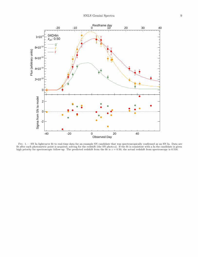
the redshift, one product of the fitting process is an es-timated redshift. We call this a “supernova photometricredshift,” or “SN photo-z,” since the redshift is estimatedfrom prior assumptions about the intrinsic brightness ofSNe Ia (0.2 mag of dispersion is allowed for in the as-sumed SN Ia properties). The SN photo-z is indepen-dent from galaxy photometric redshifts, and is useful fordeterming the telescope and instrument setup necessaryto observe key SN Ia spectroscopic features. Note thatgalaxy photometric redshifts were not used in assigningthe follow-up priority for the targets considered in thispaper.Figures 1 and 2 show examples of SN photo-z fits to

objects that were eventually confirmed to be Type Iaand Type II SNe, respectively. While we show the entirelightcurve fit here for clarity, it is apparent even beforemaximum light that the candidate in Figure 1 is likelyto be an SN Ia, while the candidate in Figure 2 is tooblue at early times to be an SN Ia. The candidates areusually spectroscopically observed near maximum light,so most SN photo-z fits are done using only the risingpart of the lightcurve.Since we observe many of our highest redshift (and

therefore spectroscopically expensive) targets at Gemini,we often apply the most strict selection critera on whatto observe there. Therefore the data from this telescopemake an excellent testbed for our selection method. How-ever, at other telescopes we observe a broader range ofcandidates to ensure that we are not missing unusual SNeIa.It is also important to note that the SN photo-z is

only used to prioritize follow-up observations – for allscientific studies we use the measured spectroscopic red-shift. The SN photo-z will be described in more detailin Sullivan et al. (2005), and the results of its implemen-tation on our SN Ia confirmation rate are given in Sec-tion 6.1.

3. OBSERVATIONAL TECHNIQUES

The observational setup and conditions for each candi-date are given in Table 1. In this section we discuss theobservational modes used in greater detail.

3.1. Instrument Setup

All supernovae were observed with the GeminiMulti Object Spectrographs (GMOS) (Hook et al. 2004).Longslit spectra of the SN candidates were taken with theGMOS R400 grating (400 lines per mm), using the 0.75′′

slit, giving a resolution of 6.9 A. The detector binning

SNLS Gemini Spectra 3

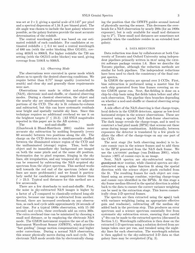
was set at 2× 2, giving a spatial scale of 0.145′′ per pixeland a spectral dispersion of 1.34 A per binned pixel. Theslit angle was chosen to include the host galaxy whereverpossible, as the galaxy features provide the most accuratedetermination of the redshift.The central wavelength used was based on our esti-

mated redshift of each candidate. For candidates at es-timated redshifts z ≤ 0.4 we used a central wavelengthof 680 nm (with the order blocking filter GG455), cov-ering 4650A to 8900A. For higher redshifts the 720 nmsetting (with the OG515 order blocker) was used, givingcoverage from 5100A to 9300A.

3.2. Observing Mode

The observations were executed in queue mode whichallows us to specify the desired observing conditions. Werequire better than 0.75′′ image quality (corrected tozenith) and clear sky and generally those requirementswere met.Observations were made in either nod-and-shuffle

(N&S), electronic nod-and-shuffle, or classical observingmodes. During a classical observation, the object andthe nearby sky are simultaneously imaged on adjacentportions of the CCD. The sky is fit column-by-columnand subtracted, but this can leave systematic residualsnear bright and spatially variable sky lines. Since thistechnique requires no additional overhead we use it onthe brightest targets (i′ ≤ 23.3). (All SNLS magnitudesreported in this paper are in the AB system.)The nod-and-shuffle mode

(Glazebrook & Bland-Hawthorn 2001) enables moreaccurate sky subtraction by nodding frequently (every60 seconds) between two positions along the slit. Thecharge on the CCD detectors is simultaneously shuffledbetween the illuminated science region of the CCD andthe unilluminated (storage) region. Thus, both theobject and its immediate sky background are imagedon both the same pixels and at the same slit position.Systematics due to pixel response, fringing in the skylines, slit irregularities, and any temporal sky variationscan be removed by subtracting the N&S acquired skyspectrum from the object spectrum. This method workswell towards the red end of the spectrum (where skylines are more problematic) and we found it particu-larly useful for candidates at magnitudes fainter thani′ > 23.3. Typical nod distances for this method are afew arcseconds.There are a few drawbacks to nod-and-shuffle. First,

the noise in sky-subtracted N&S images is higher bya factor of

√2 compared to classically-reduced long-slit

spectra, because one image is subtracted from another.Second, there are increased overheads on any observa-tion, as each nod cycle adds approximately 24 seconds ofnod time. For a typical 1800s observation, with 15 (60second) nod cycles, these overheads add an extra 360s.The extra overhead time can be minimized by choosing asmall nod distance, or by employing the electronic N&Smode. The GMOS instrument requires the use of an On-Instrument Wavefront Sensor (OIWFS), which provides“fast guiding” (image motion compensation) and higherorder corrections. During a normal N&S observation,this sensor physically moves during each nod cycle. Theelectronic N&S mode avoids this by electronically chang-

ing the position that the OIWFS guides around insteadof physically moving the sensor. This decreases the over-heads for a N&S observation by nearly 200s (for an 1800sexposure), but is only available for small nod distances(up to 2′′). These small nod distances are sometimes notpossible when the candidate resides in an extended hostgalaxy.

4. DATA REDUCTION

Data reduction was done by collaborators at both Uni-versity of Toronto and Oxford University using indepen-dent pipelines primarily written in iraf using the gem-ini software package version 1.6. Here we describe theToronto pipeline, although the reduction methods aresimilar for both pipelines. The independent reductionshave been used to check the consistency of the final out-put spectra.In GMOS the spectra are spread over 3 CCDs. First,

bias subtraction is performed using a master bias foreach chip generated from bias frames covering an en-tire GMOS queue run. Next, flat-fielding is done on achip-by-chip basis using flat-fields taken before and aftereach observation. The pipeline then branches dependingon whether a nod-and-shuffle or classical observing setupwas used.A side effect of the N&S observing is that charge-traps,

local defects in the GMOS detectors, appear as low-levelhorizontal stripes in the science observations. These areremoved using a special N&S dark-frame observation.The dark image reveals the charge-traps, and is used toconstruct a bad pixel mask (BPM) that screens out theseareas during image combination. Additionally, betweenexposures the detector is translated by a few pixels todilute the effect of the charge-traps on any one part ofthe CCD.The next stage (for both observing modes) is to lo-

cate cosmic rays in the science frames and to add themto the BPM generated from the N&S dark frame. Weuse the lacosmic package (van Dokkum 2001), whichlocates >99% of cosmic-rays in an image.Next, N&S spectra are sky-subtracted using the

gnsskysub iraf routine, while classical spectra are sky-subtracted using a spline function fit along the spatialdirection with the science object pixels excluded fromthe fit. The resulting frames for each object are com-bined using an average combine, rejecting charge-trapsand cosmic rays identified in the BPMs. At this stage asky frame median-filtered in the spatial direction is addedback to the data to ensure the correct variance weightingcan be used in the extraction stage. This leaves cosmet-ically clean 2-D spectral frames.The spectra are then extracted using the apall task

with variance weighting (using an appropriate effectivegain and readnoise), subtracting off the median skyadded back in the previous step. This produces an errorspectrum and a science spectrum essentially free fromsystematic sky subtraction errors, ensuring that carefulχ2 fits can be made to the extracted spectra (discussed inSection 5.1). Wavelength calibration is then done on theextracted 1-D spectrum using a solution derived from arclamps taken once per run, and tweaked using the night-sky lines for each observation. The wavelength solutionis then applied to the sky-subtracted 2-D data so thatgalaxy lines may be overplotted (Fig. 3).

4 Howell

The final steps are flux calibration on the extracted 1-Dspectrum, combined with a telluric correction (based onstandard star spectra), and atmospheric extinction cor-rection derived from the effective airmass of observationand the Mauna Kea extinction curve of Krisciunas et al.(1987). The spectra from the 3 chips are then combinedinto one spectrum, and an error spectrum is simultane-ously created. The chip gaps are effectively weighted tozero so that they have no influence on the χ2 fitting.

5. SN CLASSIFICATION

When possible, the slit was placed through both theSN and the center of the host galaxy. In these casesthe redshift was determined from lines in the host galaxyspectrum. Even if the host and the object are completelyblended, it is still possible to identify the host galaxy linesas they are narrower than SN features. Sky-subtracted,wavelength calibrated, combined two-dimensional spec-tra were created for each candidate and the positionsof common galaxy spectral features were overplotted, asshown in Figure 3. The lines used to identify the redshiftof each host galaxy are identified in the last column ofTable 2. In some cases the host galaxy was too faint andthe redshift was determined from the SN spectrum.Type Ia SNe can be identified by a lack of hydrogen in

their spectra, combined with broad (several thousand kms−1) P-Cyngi lines of elements such as Si II, S II, Ca II,Mg II, blends of Fe-peak lines, and sometimes Ti II, O I,or Fe III. See Filippenko (1997) for a review of SN clas-sification, and Hook et al. (2005), Lidman et al. (2005),Matheson et al. (2005), and Coil et al. (2000) for partic-ular issues and techniques associated with classificationof high-redshift SNe.

5.1. χ2fitting

High-redshift SN spectra are often blended with theirhost galaxies, so determining the SN type can be a chal-lenge (at high redshift the galaxies have a smaller an-gular size, so a greater fraction of the host light is cov-ered by the SN point-spread function). Some studiesdo not attempt to separate SN and host galaxy light,but use a cross-correlation technique to identify SNe(Matheson et al. 2005). Other authors attempt to sep-arate SN and host galaxy light using point source de-convolution (Blondin et al. 2005). Here we use a χ2 fit-ting technique to separate SN from host galaxy lightand determine the SN type. It was first developedby Howell & Wang (2002) and subsequently used byLidman et al. (2005) and Hook et al. (2005).Each SN spectrum was fit using a χ2 matching program

which compares the observed spectrum to a library oftemplate SNe of all types covering a range of epochs.The redshift, amount of host galaxy contamination, andreddening are varied to find the best fit. At a givenredshift, the code computes:

χ2 =∑ [O(λ) − aT (λ; z)10cAλ − bG(λ; z)]2

σ(λ)2,

where O is the observed spectrum, T is the SN templatespectrum, G is the host galaxy template spectrum, Aλ isthe redding law, σ is the error on the spectrum, and a,b, and c are constants that are varied to find the best fitin host galaxy, template SN, and reddening space. If the

redshift was not fixed, this equation is then reevaluatedover a range of redshifts to find the minimum χ2 in red-shift space. We use the reddening law of Cardelli et al.(1989) and RV = 3.1.If the host galaxy spectrum free of SN light could be

extracted, then it was used as the galaxy spectrum sub-tracted in the fitting process. If no galaxy contaminationwas evident, then no host was subtracted in the fit. Forother cases, template galaxies from Kinney et al. (1996)and Fioc & Rocca-Volmerange (1997) were subtracted.In cases where the Hubble type could be estimated fromimaging, the galaxy spectral energy distribution, or nar-row galaxy lines, the galaxy type was restricted in thefitting procedure. The SN template library includes 184SN Ia spectra, 75 SN Ib/c spectra, and 47 SN II spec-tra. The spectra were chosen to have good S/N, to spanthe widest possible range of epochs, to have the widestpossible wavelength coverage, and to represent all knownSN subtypes.The χ2 fitting program produces a list of the best

matching SN templates, host galaxy templates, redshifts,and reddening. As in SN detection, it is not yet possi-ble to fully automate this process – a human must stillinspect the results and make the ultimate determinationof the SN type. The type of the SN is estimated andplaced into one of six categories reflecting the type anduncertainty in the classification (Section 5.2; Fig. 4).The spectroscopic epoch is determined from the weightedmean of the best 5 epochs (weighted by the χ2 of eachfit). The average of several epochs was chosen to di-lute the effect of outliers, and to help smooth out thediversity in SN Ia spectra. The exact number of epochsaveraged has little effect on the result, since the averageis weighted by the χ2 of each fit — the best few fits willbe the dominant contributors to the average. We findχ2 = 1 for an error of σ = 2.5 days on the spectroscopicdate determination.”

5.2. SN Ia confidence index

Two factors make it harder to classify SNe at highredshift as compared to their counterparts at low red-shift: they generally have lower signal-to-noise spectraand there is a greater degree of contamination from thehost galaxy. While many classifications are obvious, oth-ers have a degree of uncertainty associated with them.To quantify this, after examination of its spectrum wegive each SN a SN Ia confidence index:

5 Certain Ia: The spectrum shows distinctive fea-tures of an SN Ia such as Si II or S II. Often Si II6150A and S II 5400A are redshifted out of the ob-served spectral range, so Si II 4000A is used as thekey indictor for SNe Ia. However, at some phases,or for some SN Ia subtypes (e. g. SN 1991T), Si II4000A would not be expected. In these cases thecandidate can be classified as a category 5 if thespectrum is an exact match to the overall spectralenergy distribution (SED) of an SN Ia (at the phaseindicated by the lightcurve) and no other type ofSN matches.

4 Highly probable Ia: The spectrum is a matchto a Ia, but lacks an unambiguous detection of oneof the features that is unique to SNe Ia (Si II or

SNLS Gemini Spectra 5

S II). Other SN types do not match the spectrumwell. These candidates usually have another pieceof confirming evidence, such as a lightcurve consis-tent with a SN Ia at the measured redshift, or theyare found in an E or S0 galaxy.

3 Probable Ia: The spectrum matches an SN Iabetter than any other SN type, but another SNtype (usually SNe Ic) is not ruled out from the spec-trum alone. This is either because the spectrumhas low S/N or because other SNe look similar atthe same phase. These candidates have a lightcurveconsistent with an SN Ia at the measured redshift,and the spectrum has a phase consistent with thelightcurve. These SNe are denoted as Ia*, followingthe notation of Lidman et al. (2005).

2 Unknown: The type cannot be determined fromthe spectrum. Often the spectrum has low signal-to-noise, or there is too much host galaxy contam-ination to make a reliable determination.

1 Probably not a Ia: The spectrum has featuresmarginally inconsistent with an SN Ia, but the typecannot be unambiguously determined.

0 Not a Ia: The spectral features are inconsistentwith a SN Ia. In this case the spectrum can usuallybe identified as an SN II, SN Ib/c, or an AGN(though note that there are no clear cases of AGNfrom Gemini spectra — these were screened out inadvance).

The primary means of classification ibfinpstws the SNspectrum, although we use all information available tosupplement this including the lightcurves, colors, andthe agreement between lightcurve phase and the spec-troscopic phase determined from the fitting process. Forexample, if the type cannot be determined from the spec-trum it would normally be classified as index 2. But ifthe lightcurves are also inconsistent with the lightcurve ofan SN Ia, then it would be moved into index 1 or 0. Thehost galaxy spectrum is never used on its own to classifya candidate, but if the host is clearly an elliptical galaxy,then this information may be used in conjunction withthe candidate spectrum and the lightcurve to solidify thestatus of a candidate as a probable SN Ia. We empha-size that the lightcurve alone is never used to classify anSN Ia – for a candidate to have a classification of SN Iaor SN Ia* it must have a spectrum matching with theexpected spectral energy distribution of an SN Ia at thephase determined from the lightcurve.One representative spectrum from each category is

shown in Figure 4. All spectra discussed in this paperare available in the online version of this article.

6. RESULTS

The SNLS officially started in June 2003 (there was apresurvey ramp-up to full operations), and we began us-ing Gemini-N and S to observe SN candidates in August2003 (semester 2003B). We usually obtain the Geminidata within a day or two of the observations and produce“real-time” reductions. After the full calibration data isreleased at the end of a run the data are rereduced. Herewe report on the final spectroscopic reductions through

November 2004. All of the spectra used in this study areavailable in the online version of the paper.Table 2 lists properties derived from the observations of

each candidate, such as type, redshift, and epoch relativeto maximum light. Table 3 shows the distribution ofSN types with respect to host galaxy type. While it isnot always possible to extract the host galaxy separatelyand examine its SED, galaxy lines are apparent becausethey are narrower than SN features. Therefore we groupgalaxies into absorption-line galaxies and emission-linegalaxies (if a galaxy has any emission lines it is consideredan emission-line galaxy). Just as at low redshift, in oursample core-collapse SNe are never seen in absorption-line (early type) galaxies.Figure 5 is a histogram of the number of candidates of

each different type with redshift. For clarity we groupindex 0 and 1 SNe together as “Not Ia” and index 4 and5 SNe together as “Ia.” SNe with weaker classifications(index 3) are plotted separately as “Ia*.” Candidatesthat could not be identified (index 2), but whose red-shifts could be determined, are also shown. It is appar-ent that we targeted the highest redshift observations atGemini — the median redshift of SNe Ia/Ia* is 0.81. Asthe redshift increases the fraction of less secure identifi-cations rises, because for faint SNe it is hard to achievea high signal-to-noise ratio in a reasonable integrationtime. Furthermore, at the higher redshifts one must relymore on the rest-frame UV light to classify the SNe, andtemplate UV observations of all SN types are scarce.Core collapse SNe cluster at lower redshifts on the his-

togram because they are usually intrinsically fainter. Forexample, a candidate with a peak magnitude of i′ = 24could be an SN Ia at z = 0.9 or could be a Type II SNat a lower redshift.

6.1. SN photo-z results

The technique of the SN photo-z is introduced inSection 2 and described in much greater detail inSullivan et al. (2005). Here we report the result of its ap-plication on our SN Ia confirmation rate. The SNLS im-plemented the SN photo-z and improved real-time pho-tometry in March 2004, although in two cases after this(04D1dr and 04D4ft), candidates had to be observedspectroscopically before a photo-z could be obtained.When no photo-z information was available before se-lecting candidates for spectroscopy, 14/26 (54%) of thecandidates were confirmed as SNe Ia — close to pre-viosly published rates. However, when we did have an SNphoto-z to guide the decision making, the Ia confirma-tion rate jumped to 27/38 (71%). There will be alwaysbe some unidentified candidates for which it is difficultto estimate a type from spectroscopy — these may stillbe SNe Ia, but are too buried in a host, or have a spec-trum with too low S/N, to be identified. However, wherethe photo-z excels is in its power to reject candidatesthat are not SNe Ia. With no prior photo-z information,7/26 (27%) of candidates with Gemini spectroscopy werefound to be certainly not or probably not SNe Ia. Afterimplementation of the technique, only 3/38 (8%) of theobservations were certainly not or probably not SNe Ia.Another benefit of the SN photo-z is that it provides

a prediction of the time of maximum light for an SN Ia,allowing observations to be scheduled to within a fewdays of this date for maximum efficiency and minimal

6 Howell

host galaxy contamination. Figure 6 shows the distribu-tion of the SNe Ia observed by Gemini with respect tomaximum light. Ninety percent of SNe Ia were observedwithin 0.5 mag of maximum light, and over half of theSNe Ia were observed within 0.1 mag of maximum light.It is clear that the flexibility provided by queue observ-ing plays a large role in optimizing the efficiency of thespectroscopic classification of targets in the SNLS. Notethat it is not always possible to schedule observationsat maximum light because we require dark time to ob-serve such faint targets, and GMOS is not always on thetelescope and available in queue mode.

6.2. Optimal time for spectroscopy

Figure 6 also shows that the least solid classifications(index 3), labeled Ia*, were usually observed after max-imum light. SNe before maximum were almost alwaysclassified with more certainty. This is partially becauseafter maximum light, especially around +7 to +10 daysafter max, it is often difficult to distinguish between SNeIa and SNe Ic. By this time certain distinguishing SN Iafeatures, such as Si II 4000A, may no longer be apparent,and the SN Ia line velocities have decreased to the rangemore typical of those found in SNe Ic.The more uncertain classifications (SNe Ia*) often oc-

cur near maximum light, because the most difficult SNe(those at the highest redshift or with the most hostgalaxy contamination) can only be observed near max-imum light. Before or after maximum light they are sofaint that they would not be placed in the spectroscopicobserving queue.An added benefit to obtaining early spectroscopy is

that SNe Ia show the greatest diversity at early times(Li et al. 2001), when the spectroscopy is probing theouter layers of supernova. Figure 6 shows that one com-promise would be to target observations at about oneweek before maximum light. At −7d, a typical Ia is onlyabout 0.25 fainter than at peak, near enough to peakbrightness to make the observations feasible. At the sametime it would provide an opportunity to observe SNe Iawhen they show the greatest diversity and also are themost distinct from SNe Ic.This window of opportunity is very narrow, however.

At −10d a typical SN Ia is 0.75 mag fainter than at peakin the restframe B-band — still too faint compared to itshost galaxy, and by −4d SN Ia spectra have lost some oftheir diversity.

6.3. Identification in the presence of host contamination

Figure 7 shows the i′ magnitude at the time of spec-troscopy versus the percentage increase in i′ brightnessin a 6 pixel (1.12′′) diameter at the time of spectroscopy.The percentage increase is measured relative to the ref-erence image, where there is no supernova light. The i′

magnitude and percentage increase were measured fromCFHT images, interpolated to the time of spectroscopy.Typically candidates were sent to Gemini only if theywere in the magnitude range 23 < i′ < 24.5. (There aresome exceptions, especially in the D3 field, which cannotbe seen by the VLT.)It is apparent from Figure 7 that when the SN signal is

greater than that of the host galaxy, candidate identifi-cation is relatively easy — when the percentage increase

is greater than 100% the candidates were not identifiedonly 7% (2/30) of the time.Clearly, image quality (IQ) plays a role in whether or

not SNe can be successfully identified in the presenceof significant host galaxy light, as shown in Figure 8.We plot the image quality at the time of spectroscopy(determined from the Gemini acquisition image) againstthe percent increase (determined from CFHT images asdescribed above). If the IQ was better than 0.55′′, can-didates were identified 88% of the time. In good seeingthe SN light is more concentrated and can be extractedin a narrow aperture, even in the presence of host con-tamination.

6.4. Success of χ2 fitting

The χ2 matching of the SN spectrum against a hostand SN spectral template library produces more identifi-cations, more robust identifications, and greater coverageof parameter space than traditional methods (unaidedexpert matching by eye). This method works optimallywith spectra that are free from systematic deviations,and whose errors are well characterized. It works excep-tionally well with GMOS nod and shuffle data, wheresystematic effects associated with sky subtraction are al-most completely removed. Correcting the spectra for tel-luric features also helps, as does a carefully generatederror spectrum.While both the spectra in this paper and in

Lidman et al. (2005) were classified by the same per-son (DAH), here the χ2 matching software is up-graded with more template supernova and galaxy spec-tra. Lidman et al. (2005) were not able to identify anycandidates with a percentage increase below 25%, butin this work we have successfully identified several can-didates with percent increases between 15%–25%. It isunclear if this is due to software improvements, observ-ing conditions, differences in the spectrographs used, ora better selection of candidates.Figure 9 also shows that the spectroscopic epoch de-

termined by the fitting program matches well with theepoch determined from the lightcurve. Unlike the spec-tral feature age technique (Riess et al. 1997), it is impor-tant to note that this program is not specifically tunedto determine the epoch of an SN Ia, and it makes no as-sumptions that the input spectrum is a Ia (it is possiblefor it to determine the epoch of an SN Ib/c for exam-ple, although this has not been extensively tested). Wefind the remarkable result that our spectroscopic fittingtechnique can determine the epoch to within 2.5 days,despite the low S/N and significant host contaminationin this data set.

7. DISCUSSION

Before comparing these confirmation rates to previouswork, a few caveats are necessary. First, not all spec-troscopic follow-up programs have as their goal the con-firmation of candidates as SNe Ia. One may wish todetermine the types of all transients to have a better de-termination of SN rates. Or in some cases the goal maybe to spectroscopically identify SNe II, as they also havecosmological utility. While we have pursued these goalsat other telescopes, the role of Gemini has been largelyto confirm SNe Ia. Second, different programs may havedifferent criteria for what is called an SN Ia/Ia*. For

SNLS Gemini Spectra 7

example, we have lightcurve infomation available at thetime of classification, which was not always the case inprevious studies. Still, our criteria are as close as pos-sible to the criteria used in other published works. Weadopt similar criteria to that of Matheson et al. (2005),and we are using the the same human classifier (DAH)and classification program (albeit slightly upgraded) asLidman et al. (2005).Despite these caveats, it is important to have some

comparison to previous work. A comparison toLidman et al. (2005) is problematic because of the in-homogeneous nature of the sample and techniques pre-sented there. They present results from six separatesearches, some classical, and some rolling, some targetingz ∼ 0.5, and some targeting z > 1.The most appropriate comparison to this work is to

consider all searches in Lidman et al. that targeted z < 1.In this case the SN Ia/Ia* confirmation rate was 62%(median SN Ia z = 0.51). A similar SN Ia confirmationrate is found if the Lidman et al. search 4 (the rollingsearch) is excluded, but SNe followed by the SCP at alltelescopes for z < 1 are included.Since rolling searches find all SNe above some mag-

nitude cutoff, the percentage of SNe Ia in the sample islower than in a classical search. In their first two years ofoperation, ESSENCE (Matheson et al. 2005), had a 43%SN Ia/Ia? confirmation rate with a median redshift of0.43 [though in the third year the SN Ia/Ia? confirmationrate rose to ∼60% (Matheson, private communication)].Again, a direct comparison to the results presented heremay not be appropriate if the two searches have differentgoals or different criteria for counting SNe Ia, but doesmake the point that if the goal is to maximize the yieldof SNe Ia, a method like the SN photo-z is helpful.Despite the difficulties in comparing this study to pre-

vious ones as noted above, we can draw some broad con-clusions from the results. First, to make the most effi-cient use of 8–10m time it is helpful to have as much in-formation as possible before sending a target to the tele-scope. In a rolling search, more information is availableat follow-up time than in a classical search, so new tech-niques are called for. Here we have demonstrated thatby fitting the available data before spectroscopy we canimprove the SN Ia/Ia* confirmation rate over our rateswhen the technique was not applied. Our SN Ia/Ia* con-firmation rate (71%) is also an increase over comparablepreviously published rates (43%-62%), despite being at amuch higher median redshift (z=0.81 vs. z=0.4-0.5). Bymaking it possible to separate likely SNe Ia from likelycore collapse SNe before a large amount of telescope timeis invested in spectroscopy, the techniques demonstratedhere improve the success rate of all follow-up programs,no matter their goal.Over the five-year lifetime of the SNLS, the these tech-

niques will result in ∼ 170 more confirmed SNe Ia. Weaim to spectroscopically observe ∼ 1000 SN candidatesduring the survey. In the absence of the photo-z thiswould result in ∼ 540 SNe Ia, but with the photo-z wecould achieve 710 SNe Ia. This is equivalent to addinganother year to the survey.

8. CONCLUSIONS

We have demonstrated several techniques for improv-ing the yield of spectroscopically identified SNe Ia at high

redshift (0.3 ≤ z ≤ 1.0). The SN photo-z is shown toeffectively screen out non-Ia candidates before they areobserved spectroscopically. When no photometric red-shifts were available, 35% of candidates turned out to beprobably or certainly not SNe Ia after spectroscopy (CI0 or 1). With photo-z information, the non-Ia “contami-nation” rate dropped to 8%. Using the photo-z we showthat we can schedule SN observations to within a fewtenths of a magnitude of maximum light, and that theoptimal phase for SN Ia identifcation and diversity is −7days. After spectroscopy, we show that by χ2 fitting oftemplate SNe we can effectively subtract host light anddetermine the type of an SN when the SN is only 15% asbright as the host in some cases. For targets where theSN is at least as bright as the underlying host, or whenthe image quality is exceptional (better than 0.55′′), thecandidate is identified more than 90% of the time. Usingχ2 fitting we can also obtain an independent measure-ment of the spectroscopic epoch that agrees well withthe phase determined from the lightcurve.These techniques have been developed using the first

year’s observations of the highest redshift candidates ofthe SNLS at Gemini North and South. Of the candidatesobserved at Gemini, 41/64 are certain or probable SNeIa. This is roughly one-third of the spectroscopic follow-up program of the SNLS. The techniques outlined herewill add ∼ 170 more confirmed SNe Ia over the five-yearproject to discover, confirm, and follow ∼ 700 SNe Ia tomeasure the equation of state of Dark Energy.

The SNLS collaboration gratefully acknowledges theassistance of Pierre Martin and the CFHT Queued Ser-vice Observations team. Jean-Charles Cuillandre andKanoa Withington were also indispensable in makingpossible real-time data reduction at CFHT. We alsothank Gemini queue observers and support staff, espe-cially Inger Jørgensen, Kathy Roth, Percy Gomez, andMarcel Bergmann, for both taking the data presentedin this paper and making observations available quickly.Canadian collaboration members acknowledge supportfrom NSERC and CIAR; French collaboration membersfrom CNRS/IN2P3, CNRS/INSU and CEA; PortugueseCollaboration members acknowledge support from FCT-Fundacao para a Ciencia e Tecnologia.SNLS relies on observations with MegaCam, a joint

project of CFHT and CEA/DAPNIA, at the Canada-France-Hawaii Telescope (CFHT) which is operated bythe National Research Council (NRC) of Canada, theInstitut National des Science de l’Univers of the CentreNational de la Recherche Scientifique (CNRS) of France,and the University of Hawaii. This work is based in parton data products produced at the Canadian AstronomyData Centre as part of the Canada-France-Hawaii Tele-scope Legacy Survey, a collaborative project of the Na-tional Research Council of Canada and the French Centrenational de la recherche scientifique.This work is also based on observations obtained at

the Gemini Observatory, which is operated by the Asso-ciation of Universities for Research in Astronomy, Inc.,under a cooperative agreement with the NSF on behalfof the Gemini partnership: the National Science Founda-tion (United States), the Particle Physics and AstronomyResearch Council (United Kingdom), the National Re-

8 Howell

search Council (Canada), CONICYT (Chile), the Aus-tralian Research Council (Australia), CNPq (Brazil) andCONICET (Argentina). This research used observa-

tions from Gemini program numbers: GN-2004B-Q-16,GS-2004B-Q-31, GN-2004A-Q-19, GS-2004A-Q-11, GN-2003B-Q-9, and GS-2003B-Q-8.

REFERENCES

Blondin, S., Walsh, J. R., Leibundgut, B., & Sainton, G. 2005,A&A, 431, 757

Cardelli, J. A., Clayton, G. C., & Mathis, J. S. 1989, ApJ, 345, 245Coil, A. L., Matheson, T., Filippenko, A. V., Leonard, D. C.,

Tonry, J., Riess, A. G., Challis, P., Clocchiatti, A., Garnavich,P. M., Hogan, C. J., Jha, S., Kirshner, R. P., Leibundgut, B.,Phillips, M. M., Schmidt, B. P., Schommer, R. A., Smith, R. C.,Soderberg, A. M., Spyromilio, J., Stubbs, C., Suntzeff, N. B., &Woudt, P. 2000, ApJ, 544, L111

Filippenko, A. V. 1997, ARA&A, 35, 309Fioc, M., & Rocca-Volmerange, B. 1997, A&A, 326, 950Glazebrook, K., & Bland-Hawthorn, J. 2001, PASP, 113, 197Hook, I., et al. 2005, AJ, submittedHook, I. M., Jørgensen, I., Allington-Smith, J. R., Davies, R. L.,

Metcalfe, N., Murowinski, R. G., & Crampton, D. 2004, PASP,116, 425

Howell, D. A., & Wang, L. 2002, Bulletin of the AmericanAstronomical Society, 34, 1256

Kinney, A. L., Calzetti, D., Bohlin, R. C., McQuade, K., Storchi-Bergmann, T., & Schmitt, H. R. 1996, ApJ, 467, 38

Krisciunas, K., Sinton, W., Tholen, K., Tokunaga, A., Golisch, W.,Griep, D., Kaminski, C., Impey, C., & Christian, C. 1987, PASP,99, 887+

Li, W., Filippenko, A. V., Treffers, R. R., Riess, A. G., Hu, J., &Qiu, Y. 2001, ApJ, 546, 734

Lidman, C., Howell, D. A., Folatelli, G., Garavini, G., Nobili, S.,Aldering, G., Amanullah, R., Antilogus, P., Astier, P., Blanc,G., Burns, M. S., Conley, A., Deustua, S. E., Doi, M., Ellis, R.,Fabbro, S., Fadeyev, V., Gibbons, R., Goldhaber, G., Goobar, A.,Groom, D. E., Hook, I., Kashikawa, N., Kim, A. G., Knop, R. A.,Lee, B. C., Mendez, J., Morokuma, T., Motohara, K., Nugent,P. E., Pain, R., Perlmutter, S., Prasad, V., Quimby, R., Raux,J., Regnault, N., Ruiz-Lapuente, P., Sainton, G., Schaefer, B. E.,Schahmaneche, K., Smith, E., Spadafora, A. L., Stanishev, V.,Walton, N. A., Wang, L., Wood-Vasey, W. M., & Yasuda (TheSupernova Cosmology Project), N. 2005, A&A, 430, 843

Matheson, T., Blondin, S., Foley, R. J., Chornock, R., Filippenko,A. V., Leibundgut, B., Smith, R. C., Sollerman, J., Spyromilio,J., Kirshner, R. P., Clocchiatti, A., Aguilera, C., Barris, B.,Becker, A. C., Challis, P., Covarrubias, R., Garnavich, P., Hicken,M., Jha, S., Krisciunas, K., Li, W., Miceli, A., Miknaitis, G.,Prieto, J. L., Rest, A., Riess, A. G., Salvo, M. E., Schmidt, B. P.,Stubbs, C. W., Suntzeff, N. B., & Tonry, J. L. 2005, AJ, 129,2352

Perlmutter, S., Aldering, G., Goldhaber, G., Knop, R. A., Nugent,P., Castro, P. G., Deustua, S., Fabbro, S., Goobar, A., Groom,D. E., Hook, I. M., Kim, A. G., Kim, M. Y., Lee, J. C., Nunes,N. J., Pain, R., Pennypacker, C. R., Quimby, R., Lidman,C., Ellis, R. S., Irwin, M., McMahon, R. G., Ruiz-Lapuente,P., Walton, N., Schaefer, B., Boyle, B. J., Filippenko, A. V.,Matheson, T., Fruchter, A. S., Panagia, N., Newberg, H. J. M.,Couch, W. J., & The Supernova Cosmology Project. 1999, ApJ,517, 565

Perlmutter, S., Pennypacker, C. R., Goldhaber, G., Goobar, A.,Muller, R. A., Newberg, H. J. M., Desai, J., Kim, A. G., Kim,M. Y., Small, I. A., Boyle, B. J., Crawford, C. S., McMahon,R. G., Bunclark, P. S., Carter, D., Irwin, M. J., Terlevich, R. J.,Ellis, R. S., Glazebrook, K., Couch, W. J., Mould, J. R., Small,T. A., & Abraham, R. G. 1995, ApJ, 440, L41

Pritchet, C. J., et al. 2004, ArXiv Astrophysics e-printsRiess, A. G., Filippenko, A. V., Challis, P., Clocchiatti, A., Diercks,

A., Garnavich, P. M., Gilliland, R. L., Hogan, C. J., Jha, S.,Kirshner, R. P., Leibundgut, B., Phillips, M. M., Reiss, D.,Schmidt, B. P., Schommer, R. A., Smith, R. C., Spyromilio, J.,Stubbs, C., Suntzeff, N. B., & Tonry, J. 1998, AJ, 116, 1009

Riess, A. G., Filippenko, A. V., Leonard, D. C., Schmidt, B. P.,Suntzeff, N., Phillips, M. M., Schommer, R., Clocchiatti, A.,Kirshner, R. P., Garnavich, P., Challis, P., Leibundgut, B.,Spyromilio, J., & Smith, R. C. 1997, AJ, 114, 722

Riess, A. G., Strolger, L., Tonry, J., Tsvetanov, Z., Casertano,S., Ferguson, H. C., Mobasher, B., Challis, P., Panagia, N.,Filippenko, A. V., Li, W., Chornock, R., Kirshner, R. P.,Leibundgut, B., Dickinson, M., Koekemoer, A., Grogin, N. A.,& Giavalisco, M. 2004, ApJ, 600, L163

Schlegel, D. J., Finkbeiner, D. P., & Davis, M. 1998, ApJ, 500, 525Sullivan, M., et al. 2004, ArXiv Astrophysics e-prints—. 2005, AJ, submittedvan Dokkum, P. G. 2001, PASP, 113, 1420

SNLS Gemini Spectra 9

-40 -20 0 20 40Observed Day

-2

0

2

Sig

ma

from

SN

Ia m

odel

0

2•10-10

4•10-10

6•10-10

8•10-10

1•10-9

Flu

x (a

rbitr

ary

units

)-20 -10 0 10 20 30 40

Restframe day

04D4inzph: 0.50

g’r’i’

Fig. 1.— SN Ia lightcurve fit to real-time data for an example SN candidate that was spectroscopically confirmed as an SN Ia. Data arefit after each photometric point is acquired, solving for the redshift (the SN photo-z). If the fit is consistent with a Ia the candidate is givenhigh priority for spectroscopic follow-up. The predicted redshift from the fit is z = 0.50, the actual redshift from spectroscopy is 0.516.

10 Howell

-20 0 20 40 60Observed Day

-5

0

5

10

Sig

ma

from

SN

Ia m

odel

0

2•10-10

4•10-10

6•10-10F

lux

(arb

itrar

y un

its)

-20 -10 0 10 20 30 40Restframe day

04D1mezph: 0.57

g’r’i’

Fig. 2.— A SN Ia lightcurve fit to an SN candidate that was eventually spectroscopically identified as a Type II-P. Because the dataare not a good fit to an SN Ia lightcurve, such candidates are lowered in priority for spectroscopic follow-up. Even at early times it isapparent that the candidate is not an SN Ia because it is too blue. The formal prediction for the SN photo-z (under the assumption thatthe candidate is an SN Ia) is 0.56. The spectroscopic redshift is z = 0.256 — much lower because SNe II are ∼ 1.5 mag fainter than SNeIa at a given redshift.

[SII][SII][NII]H-alpha

Fig. 3.— Section of a two-dimensional nod and shuffle sky-subtracted spectrum. The wavelength solution is applied to the 2D spectrumand the positions of common galaxy lines are overplotted. Wavelength increases to the right; the spatial direction is vertical. The supernovais blended with the host galaxy, but the galaxy emission lines are apparent as the dark diagonal lines. The galaxy lines are slanted due tothe rotation of the galaxy. Note the excellent sky subtraction – the subtracted sky lines are the vertical bands of increased poisson noise,but lack systematic residuals.

SNLS Gemini Spectra 11

5000 6000 7000 8000 9000Observed Wavelength [Å]

−0.5

0.0

0.5

1.0

1.5

2.0F

λ (n

orm

aliz

ed)

3500 4000 4500 5000 5500 6000Rest Wavelength [Å] at z=0.496

SN 1998bu −403D1ax

6000 7000 8000 9000Observed Wavelength [Å]

−2

−1

0

1

2

3

Fλ

(nor

mal

ized

)

3500 4000 4500 5000 5500Rest Wavelength [Å] at z=0.670

SN 1989B +504D4ic

6000 7000 8000 9000Observed Wavelength [Å]

−2

−1

0

1

2

3

4

Fλ

(nor

mal

ized

)

3000 3500 4000 4500Rest Wavelength [Å] at z=0.930

SN 1981B max04D1ow

5000 6000 7000 8000Observed Wavelength [Å]

0.0

0.5

1.0

1.5

2.0

Fλ

(nor

mal

ized

)

4000 4500 5000 5500 6000Rest Wavelength [Å] at z=0.380

SN 1999bn +22Sc galaxy04D1jf04D1jf original data

5000 6000 7000 8000 9000Observed Wavelength [Å]

−2

−1

0

1

2

3

Fλ

(nor

mal

ized

)

4000 4500 5000 5500 6000 6500Rest Wavelength [Å] at z=0.364

SN 1994I max03D1cj

5000 6000 7000 8000 9000Observed Wavelength [Å]

−1.0

−0.5

0.0

0.5

1.0

1.5

2.0

Fλ

(nor

mal

ized

)

4500 5000 5500 6000 6500 7000Rest Wavelength [Å] at z=0.217

SN 1993W +2104D3ae

Fig. 4.— Spectra of SNLS candidates observed by Gemini. One spectrum from each SN Ia confidence index is shown as an example. Allother spectra are available online. When there is only minor galaxy subtraction, only the subtracted spectrum (rebinned to 5A)is shown.In cases where the galaxy subtraction is important, the original (unbinned) spectrum, the galaxy subtracted spectrum and the smoothedhost galaxy that was subtracted are shown. Top-left: 5 (Certain Ia), the Si 4000A feature is obvious; top-right: 4 (Highly probable Ia), allfeatures match, but at this phase the Si 4000A feature is not a definitive detection; middle-left: 3 (Probable Ia) an SN Ia is the best fit,but the lower S/N at high redshift leaves some room for doubt; middle-right: 2 (Unidentified), significant host contamination, combinedwith the fact that many SN types look similar at a late phase means that this SN type is uncertain, despite the match to an SN Ia shown;bottom-left: 1 (Probably not a Ia) An SN Ic is a good fit to the spectrum, but the redshift is uncertain and the S/N is too low to makea definitive classification; bottom-right: 0 (Certainly not a Ia), in this case a Type II. For Index 5, 4, 3, 1, and 0 the gray line (light blueonline) shows the data after host galaxy subtraction (if necessary), rebinned to 5A. For Index 2, the top gray line (dark green) shows theoriginal data, overplotted with the best-fit host galaxy template (bold lighter green). The lower gray line (light blue) shows the data afterhost subtraction and rebinning — the SN type could not be identified.

12 Howell

0

5

10

15

Num

ber

per

bin

0.0 0.1 0.2 0.3 0.4 0.5 0.6 0.7 0.8 0.9 1.0 1.1 1.2Spectroscopic redshift

IaIa*UnidentifiedNot Ia

Fig. 5.— Histogram of the redshifts of candidates observed by Gemini, where the highest redshift candidates were usually observed.Note that SN Ia classifications are less certain (Ia*) at higher redshifts where the S/N is lower and scarce restframe UV observations mustbe used to classify the SN. Non-Ia candidates were typically at a lower redshift than that predicted for an SN Ia using the SN photo-z,since core collapse SNe are generally fainter than SNe Ia. The median redshift of SNe Ia/Ia* is 0.81.

SNLS Gemini Spectra 13

0

1

2

3

4

5

6

7

8

9

10

Num

ber

per

bin

50% w/in 0.1mag of peak

90% w/in 0.5mag of peak

-15 -10 -5 0 5 10 15 20 25Restframe time of spectoscopy relative to B max (days)

2.24 0.74 0.12 0.00 0.16 0.54 1.05 1.67 2.22Magnitude relative to max for s=1

IaIa*

Fig. 6.— Histogram of rest frame epoch relative to restframe B-band maximum light for Type Ia/Ia* SNe. Since we can predict thetime of maximum light before a candidate is sent for spectroscopy, we can plan the observations so that the contrast between the SN andthe host galaxy is at a maximum. More than 50% of SNe were observed within 0.1 mag of maximum light, and 90% of SNe were observedwithin 0.5 mag of maximum. It is easier to classify SNe Ia with certainty if spectra are taken just before maximum light.

14 Howell

10 100 1000 10000Percentage Increase

21

22

23

24

25

i(AB

) M

agni

tude

More easily identified

Significant host

Faint

Usually sent to other telescopes

Ia/Ia*UnidentifiedNot Ia

Fig. 7.— i′ Magnitude at time of spectroscopy versus percentage increase. Typically candidates were only sent to Gemini if 23 < i′ < 24.5.When the candidate is brighter than the host (greater than 100% increase) it is identified 93% of the time.

SNLS Gemini Spectra 15

10 100 1000 10000Percentage Increase

0.4

0.6

0.8

1.0

1.2

1.4

Imag

e Q

ualit

y (a

rcse

c)SN brighter than hostIQ less important

Easy to ID

IaIa*UnidentifiedNot Ia

Fig. 8.— Image quality (IQ) at the time of spectroscopy versus percentage increase at the time of spectroscopy. If the SN was brighterthan the host (% increase > 100), IQ plays a less significant role in determining whether a candidate is identified. However, candidatescan still be identified in the presence of significant host contamination if the seeing is exceptional. If the IQ was less than 0.55′′ candidateswere identified 88% of the time (only SNe with both a percentage increase and IQ measurement are plotted in the figure).

16 Howell

-15 -10 -5 0 5 10 15LC Epoch (days)

-15

-10

-5

0

5

10

15

Spe

ctro

scop

ic E

poch

(da

ys)

Fig. 9.— Rest frame epoch of spectroscopy relative to rest B-band maximum light as determined by fits to the lightcurve and fits to thespectra. The line shows where SNe should lie if the lightcurve epoch is equal to the spectroscopic epoch – it is not a fit to the data. Thelightcurve epoch is from fits to the final reductions of the lightcurve data where possible, but in some cases it is from fits to preliminary(real-time) data. The open circle is a spectroscopically peculiar (SN 2001ay-like) SN for which there are few templates in the spectroscopicmatching library. The inset shows the difference between the spectroscopic epoch and the lightcurve epoch as a function of lightcurveepoch, with the same units as the larger graph. Note that from -4d to +4d, SN Ia spectra are similar, so an automatic determination ofa date from fits to the spectrum can be difficult. There is also a tendency to overpredict the spectroscopic phase at early times. This isprobably due to the scarcity of early SN Ia spectra.

SNLS Gemini Spectra 17

TABLE 1SNLS SN Candidates Observed with Gemini

SN RA (2000) Dec (2000) UT Date Exp.a Modeb λcc IQd Mage %If

03D1as 02:24:24.520 -04:21:40.19 2003-09-27 6000 N+S 720 0.41 23.96 147503D1ax 02:24:23.320 -04:43:14.41 2003-09-29 2400 C 720 0.61 23.16 6503D1bk 02:26:27.410 -04:32:11.99 2003-09-28 4800 N+S 720 0.47 23.95 8303D1cj 02:26:25.081 -04:12:39.89 2003-10-26 5400 N+S 720 0.57 24.11 7603D1cm 02:24:55.288 -04:23:03.68 2003-10-27 5400 N+S 720 0.72 23.77 97003D1co 02:26:16.238 -04:56:05.76 2003-11-01 7200 N+S 720 0.84 23.64 18803D1ew 02:24:14.088 -04:39:56.98 2003-12-21 7200 N+S 720 0.71 23.76 166103D1fp 02:26:03.073 -04:08:02.02 2003-12-26 7200 N+S 720 0.55 23.86 3003D1fq 02:26:55.683 -04:18:08.10 2003-12-24 5400 N+S 720 0.48 23.59 4103D4cj 22:16:06.660 -17:42:16.72 2003-08-26 2700 C 680 0.83 21.85 1000003D4ck 22:15:08.910 -17:56:02.17 2003-08-27 2400 C 680 0.46 22.78 190503D4cn 22:16:34.600 -17:16:13.55 2003-08-27 4800 C 720 0.46 23.81 4903D4cy 22:13:40.460 -17:40:53.90 2003-09-26 5400 N+S 720 0.59 24.19 14903D4cz 22:16:41.870 -17:55:34.54 2003-09-27 3600 C 720 0.41 24.41 1503D4fd 22:16:14.471 -17:23:44.37 2003-10-24 3600 N+S 720 0.67 23.61 32103D4fe 22:16:08.844 -17:55:19.21 2003-10-24 3600 N+S 720 0.48 23.58 6603D4gl 22:14:44.177 -17:31:44.47 2003-10-29 3600 N+S 720 0.63 23.43 12104D1de 02:26:35.925 -04:25:21.65 2004-08-17 7200 N+S 720 0.51 23.63 5604D1dr 02:27:23.905 -04:51:27.43 2004-08-14 5400 N+S 720 0.57 24.28 7204D1hd 02:26:08.850 -04:06:35.22 2004-09-13 2400 C 680 0.85 22.16 125404D1ho 02:24:44.856 -04:39:15.55 2004-09-16 3600 C 720 0.59 23.13 2404D1hy 02:24:08.678 -04:49:52.22 2004-09-11 5400 N+S 720 0.73 23.53 99604D1jf 02:25:18.914 -04:49:09.05 2004-10-13 2400 C 680 0.92 22.94 1904D1ln 02:25:53.482 -04:27:03.75 2004-10-17 2400 C 680 0.62 22.80 2904D1ow 02:26:42.708 -04:18:22.55 2004-11-08 5400 N+S 720 0.69 23.87 420104D2aag 10:02:02.100 +02:40:51.76 2004-01-23 7320 N+S 720 0.58 24.19 · · ·

04D2adg 10:00:08.093 +02:39:01.40 2004-01-22 7320 N+S 720 0.54 24.17 · · ·

04D2aeg 10:01:52.414 +02:13:21.11 2004-01-21 5490 N+S 720 0.75 23.64 · · ·

04D3aa 14:16:49.935 +52:45:31.12 2004-01-30 5400 N+S 720 1.02 24.05 1204D3ae 14:22:21.569 +52:21:39.21 2004-01-25 2400 C 680 0.94 23.10 19604D3ax 14:22:39.072 +52:51:52.57 2004-01-28 5400 N+S 720 1.30 24.95 24604D3bf 14:17:45.096 +52:28:04.31 2004-02-17 2700 C 680 · · · 23.16 · · ·

04D3dd 14:17:48.431 +52:28:14.72 2004-04-25 5400 N+S 720 0.59 24.06 37504D3de 14:22:13.503 +52:17:09.71 2004-04-27 7200 N+S 720 0.57 24.01 65104D3fj 14:19:50.703 +52:41:31.84 2004-04-28 7200 N+S 720 0.72 24.19 10804D3fq 14:16:57.906 +52:22:46.53 2004-04-26 5400 N+S 720 0.97 23.04 41204D3gu 14:22:07.359 +52:38:54.60 2004-05-22 4800 C 720 1.03 22.60 604D3gx 14:20:13.678 +52:16:58.60 2004-05-21 7200 N+S 720 0.40 24.38 243904D3hn 14:22:06.878 +52:13:43.46 2004-05-22 4800 C 720 0.47 22.94 1404D3kr 14:16:35.937 +52:28:44.20 2004-06-16 2400 C 680 0.82 21.60 15604D3lp 14:19:50.927 +52:30:11.85 2004-05-27 5400 N+S 720 0.52 24.45 7804D3lu 14:21:08.009 +52:58:29.74 2004-06-23 3600 N+S 720 0.84 23.49 1704D3mk 14:19:25.830 +53:09:49.56 2004-06-19 4320 N+S 720 1.25 23.27 8604D3ml 14:16:39.107 +53:05:35.66 2004-06-20 3600 N+S 720 0.41 23.90 225204D3nc 14:16:18.224 +52:16:26.09 2004-07-13 2400 C 720 0.66 23.39 14904D3nh 14:22:26.729 +52:20:00.92 2004-06-23 1800 C 680 0.80 21.66 19904D3nq 14:20:19.193 +53:09:15.90 2004-07-14 1500 C 680 0.61 21.03 1000004D3nr 14:22:38.526 +52:38:55.89 2004-07-15 7200 N+S 720 0.69 24.40 230004D3ny 14:18:56.332 +52:11:15.06 2004-07-10 5400 N+S 720 0.79 23.23 20304D3oe 14:19:39.381 +52:33:14.21 2004-07-11 3600 N+S 720 0.62 23.21 2804D3og 14:20:39.748 +53:01:15.02 2004-07-19 2700 C 720 1.10 21.81 15104D3pd 14:22:33.506 +52:13:47.77 2004-07-18 3600 N+S 720 0.83 23.34 7204D4dm 22:15:25.470 -17:14:42.71 2004-07-18 3600 N+S 720 0.96 23.55 12304D4ec 22:16:29.286 -18:11:04.13 2004-07-19 3600 N+S 720 0.70 23.08 3704D4ft 22:14:31.097 -17:40:19.74 2004-08-12 3600 C 720 0.67 23.21 7804D4gg 22:16:09.268 -17:17:39.98 2004-08-16 3600 C 720 0.81 23.03 3004D4hu 22:15:36.193 -17:50:19.81 2004-09-18 5400 N+S 720 0.52 23.45 8404D4hx 22:13:40.587 -17:23:03.35 2004-09-16 5400 N+S 720 0.73 24.15 2504D4ic 22:14:21.841 -17:56:36.43 2004-09-12 5160 N+S 720 0.69 23.34 23104D4ih 22:17:17.041 -17:40:38.74 2004-10-07 5400 N+S 720 0.52 23.95 4104D4ii 22:15:55.645 -17:39:27.09 2004-09-15 7200 N+S 720 0.45 23.86 5704D4im 22:15:00.885 -17:23:45.84 2004-10-10 7200 N+S 720 0.44 23.23 1804D4jy 22:13:51.605 -17:24:18.13 2004-10-14 8881 N+S 720 0.77 24.08 177904D4kn 22:15:04.324 -17:19:45.05 2004-10-19 5400 N+S 720 0.60 23.74 97

Note. — SNe observed using Gemini GMOS during semesters 2003B, 2004A, and 2004B. Observa-tions from Gemini-N except where noted. Observational setup: R400 Grating, 0.75′′slit, binning 2×2.One observation is not listed in this table, SNLS 04D3bf, because it was observed at Gemini-S afterthe SN had faded to get the host redshift.aExposure time in seconds.bObserving mode: nod and shuffle or classical.cCentral wavelength of observing setup in nm.dImage Quality in arcseconds.ei′(AB) magnitude at time of spectroscopy.fPercent increase in a 1.12′′ diameter aperture at position of candidate at time of spectroscopy

compared to the flux at the same position in the reference image.gObserved at Gemini-S.

18 Howell

TABLE 2Derived properties for SNLS SN Candidates Observed with Gemini.

SN z ± Type CIa τLCb

± τspecc z from

03D1as 0.872 0.001 SN: 2 · · · · · · · · · O II:03D1ax 0.496 0.001 SN Ia 5 -3.0 0.1 -3.3 H&K03D1bk 0.8650 0.0005 SN Ia 5 -6.3 0.1 -2.1 H&K, Hβ, Hγ03D1cj 0.364 0.001 SN Ib/c: 1 · · · · · · · · · Hα, O III

03D1cm 0.87 0.02 SN Ia 4 -5.0 0.3 2.4 SN03D1co 0.68 0.01 SN Ia 5 -4.8 0.3 -1.2 SN03D1ew 0.868 0.001 SN Ia 5 0.9 0.4 -0.2 O II

03D1fp 0.270 0.001 SN IIb 0 · · · · · · · · · Hα, Hβ, N II, O II, S II

03D1fq 0.80 0.02 SN Ia 4 -1.6 0.3 2.2 SN03D4cj 0.27 0.01 SN Ia 5 -9.7 0.1 -6.9 SN03D4ck 0.189 0.001 SN IIn 0 · · · · · · · · · SN03D4cn 0.818 0.001 SN Ia 4 -0.5 0.6 2.8 O II, O III, Hβ03D4cy 0.9271 0.0005 SN Ia 4 5.3 0.3 7.7 O II

03D4cz 0.695 0.001 SN Ia 4 9.4 0.1 8.7 H&K, G-band03D4fd 0.791 0.003 SN Ia 5 -1.6 0.3 -1.5 O II

03D4fe ? · · · SN: 1 · · · · · · · · · · · ·

03D4gl 0.56 0.01 SN Ia 4 -9.0 0.2 -6.0 SN04D1de 0.7677 0.0002 SN Ia* 3 -6.8 0.1 -4.5 O II, O III, Hβ, poss H&K04D1dr 0.6414 0.0003 SN: 2 · · · · · · · · · O II, O III, Hβ, Hγ04D1hd 0.3685 0.0005 SN Ia 5 -4.8 0.1 -4.0 O III, weak O II

04D1ho 0.7012 0.0004 SN 2 · · · · · · · · · O II, O III, H&K, Hβ, Hγ04D1hy 0.85 0.02 SN Ia 5 -3.5 0.3 -3.2 SN04D1jf 0.3800 0.0002 SN: 2 · · · · · · · · · O II, O III, Hβ04D1ln 0.2072 0.0002 SN II-P 0 · · · · · · · · · Hα, N II, S II

04D1ow 0.93 0.02 SN Ia 4 2.6 0.2 -0.8 SN04D2aag ? · · · SN: 2 · · · · · · · · · · · ·

04D2adg 0.6802 0.0002 SN: 2 · · · · · · · · · O II, O III, Hβ04D2aeg 0.843 0.001 SN Ia 4 0.0 0.1 -1.5 H&K04D3aa 0.2045 0.0002 SN II 0 · · · · · · · · · Hα, Hβ, O III, S II

04D3ae 0.217 0.001 SN II 0 · · · · · · · · · Hα, O III

04D3ax 0.3558 0.0002 SN II: 1 · · · · · · · · · Hα, Hβ, O III

04D3bf 0.1560 0.0005 SN Ia 5 · · · · · · 15.1 O II, O III, S II, Hα, Hβ04D3dd 1.01 0.02 SN Ia 4 2.9 0.3 -1.4 SN04D3de ? · · · SN II-P 0 · · · · · · · · · · · ·

04D3fj ? · · · SN: 1 · · · · · · · · · · · ·

04D3fq 0.73 0.01 SN Ia 4 0.8 0.3 3.6 SN04D3gu 0.748 0.001 SN: 2 · · · · · · · · · H&K, Balmer, weak O II

04D3gx 0.91 0.02 SN Ia* 3 10.8 0.2 8.3 SN04D3hn 0.5516 0.0003 SN Ia 5 7.2 0.1 4.9 H&K, Balmer04D3kr 0.3373 0.0002 SN Ia 5 4.4 0.1 1.7 O II, O III, Hβ04D3lp 0.983 0.001 SN Ia* 3 1.0 0.2 -1.2 O II

04D3lu 0.8218 0.0002 SN Ia 4 5.5 0.1 5.6 H&K04D3mk 0.813 0.001 SN Ia 5 -2.4 0.1 1.2 O II, H&K04D3ml 0.95 0.02 SN Ia 4 -1.8 0.3 1.1 SN04D3nc 0.817 0.001 SN Ia* 3 7.2 0.2 · · · poss O II

04D3nh 0.3402 0.0002 SN Ia 5 3.5 0.1 3.7 Hα, Hβ, O II, poss H&K04D3nq 0.22 0.01 SN Ia 5 8.1 0.1 8.8 SN04D3nr 0.96 0.02 SN Ia* 3 8.1 0.3 3.9 SN04D3ny 0.81 0.02 SN Ia 5 1.6 0.2 2.5 SN04D3oe 0.756 0.001 SN Ia 4 1.4 0.1 1.8 H&K04D3og 0.352 0.001 SN 2 · · · · · · · · · Hα, Hβ, O II, N II, S II

04D3pd 0.760 0.001 SN: 2 · · · · · · · · · Hβ, O II, O III

04D4dm 0.811 0.001 SN Ia 4 2.7 0.2 -0.7 O II, O III

04D4ec 0.593 0.001 SN: 2 · · · · · · · · · O II, O III, Hβ, Hγ04D4ft 0.2666 0.0002 SN 2 · · · · · · · · · O III, Hα, Hβ04D4gg 0.4238 0.0004 SN Ia 5 -9.7 0.1 -10.0 O II, O III, Hα, Hβ, Hγ04D4hu 0.7027 0.0003 SN Ia 5 5.2 0.5 5.0 O II, O III, Hβ

04D4hx 0.545 0.005 SN: 2 · · · · · · · · · 4000A break, poss H&K04D4ic 0.68 0.02 SN Ia 4 2.5 0.3 4.8 SN04D4ih 0.934 0.001 SN Ia* 3 8.7 0.2 5.6 O II, H&K, some Balmer04D4ii 0.866 0.001 SN Ia 5 -4.6 0.2 -3.5 O II

04D4im 0.7510 0.0005 SN Ia 4 0.7 0.2 0.2 H&K, Hδ04D4jy 0.93 0.02 SN Ia* 3 2.0 0.4 0.0 SN04D4kn 0.9095 0.0005 SN: 2 · · · · · · · · · O II, H&K, Balmer

Note. — Derived properties for SNe listed in Table 1. A colon denotes uncertainty.aSN Ia confidence index: (5) Certain Ia; (4) Highly probable Ia; (3) Probable Ia; (2) Unidentified;

(1) Probably not a Ia; (0) Certainly not a Ia.bEpoch determined from lightcurve: Rest frame epoch at which spectroscopy was taken relativeto rest frame B-band maximum light.cEpoch determined from spectroscopic fit. The uncertainty on this value is 2.5 days.

SNLS Gemini Spectra 19

TABLE 3Ia Confidence Index and

Host Type.

CIa Abs.b Emis.c Noned

5 2 11 54 5 3 83 0 4 32 1 11 11 0 2 20 0 4 2

Note. — Note that probableand certain core collapse SNe (in-dex 0 and 1) do not occur in ab-sorption line galaxies.aIa confidence index: (5) Cer-

tain Ia; (4) Highly probable Ia;(3) Probable Ia; (2) Unidentified;(1) Probably not a Ia; (0) Cer-tainly not a Ia.bHosts have only absorptionlines.cHosts have emission features.dCandidates with no host fea-tures, either because there was noapparent host or because the slitcould not be placed through thegalaxy.