arX

iv:0

711.

4104

v1 [

astr

o-ph

] 2

6 N

ov 2

007

Draft version October 26, 2018Preprint typeset using LATEX style emulateapj v. 08/22/09

TESTS OF THE RADIAL TREMAINE-WEINBERG METHOD

Sharon E. Meidt and Richard J. RandDepartment of Physics and Astronomy,

University of New Mexico, 800 Yale Blvd Northeast, Albuquerque, NM 87131

Michael R. MerrifieldUniversity of Nottingham, School of Physics & Astronomy, University Park, Nottingham, NG7 2RD

Victor P. DebattistaCentre For Astrophysics, University of Central Lancashire, Preston, UK PR1 2HE

and

Juntai ShenMcDonald Observatory, The University of Texas at Austin, 1 University Station, C1402, Austin, TX 78712

Draft version October 26, 2018

ABSTRACT

At the intersection of galactic dynamics, evolution and global structure, issues such as the rela-tion between bars and spirals and the persistence of spiral patterns can be addressed through thecharacterization of the angular speeds of the patterns and their possible radial variation. The RadialTremaine-Weinberg (TWR) Method, a generalized version of the Tremaine-Weinberg method for ob-servationally determining a single, constant pattern speed, allows the pattern speed to vary arbitrarilywith radius. Here, we perform tests of the TWR method with regularization on several simulatedgalaxy data sets. The regularization is employed as a means of smoothing intrinsically noisy solutions,as well as for testing model solutions of different radial dependence (e.g. constant, linear or quadratic).We test these facilities in studies of individual simulations, and demonstrate successful measurementof both bar and spiral pattern speeds in a single disk, secondary bar pattern speeds, and spiral winding(in the first application of a TW calculation to a spiral simulation). We also explore the major sourcesof error in the calculation and find uncertainty in the major axis position angle most dominant. Inall cases, the method is able to extract pattern speed solutions where discernible patterns exist towithin 20% of the known values, suggesting that the TWR method should be a valuable tool in thearea of galactic dynamics. For utility, we also discuss the caveats in, and compile a prescription for,applications to real galaxies.Subject headings: galaxies: spiral – galaxies: kinematics and dynamics – galaxies: structure – methods:

numerical

1. INTRODUCTION

One of the prime unresolved issues in the dynam-ics and evolution of galaxy disks remains the originand evolution of large-scale bar and spiral structure.Though the persistence of grand-design spirals has beentied observationally to the presence of bars or compan-ions (Kormendy & Norman 1979), virtually nothing isknown about the actual lifetimes of spiral patterns. Ad-ditionally, despite indications that the relation betweenbar and spiral pattern speeds (which Sellwood & Sparke(1988) first argued may not be equal) may be im-portant for understanding the role of bars in angularmomentum transfer during secular disk evolution (e.g.Debattista & Sellwood 1998 and Debattista & Sellwood2000), there are as yet unanswered questions about theconnections between multiple patterns in different radialzones. While mode-coupling between patterns, whichallows efficient outward angular momentum transfer indisks (Sygnet et al. 1999; Masset & Tagger 1997) seemsa most promising link, in 2D N-body simulations with adissipative gas component Rautiainen & Salo (1999) findevidence for spiral structure in the absence of a bar, bar-

spiral mode coupling, spiral-spiral mode coupling, andmultiple pattern speeds without mode coupling.Clearly, to address questions about the persistence of

spiral patterns and the relation between bars and spiralsrequires not only determination of the pattern speed buthow it varies with radius; only with accurate measure-ment of bar and spiral or inner and outer spirals patternspeeds in the same galaxy can we confirm whether spiralstructure is steady or winding, whether bars and spiralpattern speeds are equal or are unrelated, whether mode-coupling exists, and the domain and number of patternsthat can be sustained in a disk.Because they are not directly accessible through ob-

servation, pattern speeds are often determined with in-direct means such as the identification of predicted be-havior at resonance radii (e.g. Elmegreen et al. 1989;Elmegreen et al. 1996) or kinematic and morphologicalcomparisons of simulated and observed structure (e.g.Rautiainen et al. 2005; Garcia-Burillo et al. 1993). It isalso clearly desirable to employ methods for estimatingpattern speeds which do not rely on theoretical mod-els or simulation. Many other pattern speed determina-tions have therefore centered on the use of the model-

2

independent method of Tremaine & Weinberg (1984;hereafter TW) which presents a rigorous derivation forthe pattern speed Ωp based on the requirement of conti-nuity using observationally accessible quantities. The de-termination of Ωp involves surface density-weighted posi-tion and velocity line integrals parallel to the galaxy ma-jor axis under several essential assumptions. Specifically,the method requires that the disk of the galaxy is flat(unwarped) and contains a single, well-defined rigidly-rotating pattern; that the surface density of a kinematictracer of a disk component, which must obey continuity,becomes negligibly small at some radius and all azimuthswithin the map boundary (thereby critically yielding con-verged integrals); and that the relation between the emis-sion from this component and its surface density is lin-ear, or if not, suspected deviations from linearity can bemodeled.In that information from all sampled radii is associated

with a single, constant pattern speed, the TW calcu-lation poses a challenge for extracting multiple distinctor radially varying pattern speeds. Non-axisymmetricstructures beyond a dominant pattern such as a bar inthe disk of a galaxy will interfere with the measure-ment of Ωp of the bar; when a non-axisymmetric diskcan be decomposed into two components with differentpattern speeds, then the TW estimate is a luminosity-and asymmetry-weighted average of the two patterns(Debattista, Gerhard & Sevenster 2002). The TW esti-mate for the secondary pattern speed in the inner diskof NGC 6946 observed in Hα, for example, is estimatedto be limited to an uncertainty of as much as 50% giventhe primary pattern’s contribution to the TW integrals(Fathi et al. 2007).Such issues notwithstanding, there have been several

recent adaptations of the TW method to positive ef-fect. Applications of the TW method to SB0 galaxiesusing stellar light as a tracer extend the limits of inte-gration in the TW calculation to just past the end ofthe bar in order to minimize contributions to the TW in-tegrals from non-axisymmetric (and several magnitudesdimmer) features beyond the bar; in such cases, inte-grating past the structure of interest is found to be suffi-cient for achieving converged integrals. The bar patternspeeds in NGC 7079 (Debattista & Williams 2004) andNGC 1023 (Debattista et al. 2002), for example, haveboth been successfully measured in this way.When there exist more than one pattern in distinct

radial zones, however, arguments about the convergenceof the TW integrals are less straight-forward. To mea-sure the secondary bar pattern speed in NGC 2950,Corsini et al. (2003) and Maciejewski (2006) explore de-coupling the inner secondary and outer primary bar pat-tern speeds by associating each component with uniquesurface brightness contributions in the TW calculation.The TW integrals are modified by the presence of theinner pattern based on an assumption about how andwhere the two patterns decouple (to first order). Thisanalysis has confirmed the existence of, if not measured,a unique secondary bar pattern speed possibly indicatingcounter-rotation with respect to the primary bar.At their best–improving the accuracy of pattern speed

estimates to about 20% (Gerssen & Debattista 2007)–these kinds of adaptations of the TW method for mea-surement of single or multiple patterns still require as-

sumptions about bar extent based on morphological orkinematic signatures. To separate the observed surfacebrightness in NGC 2950 into secondary and primary barscomponents, Maciejewski (2006) must assume that thepatterns indeed decouple at the inner-bar end, or thatthe outer pattern is axially symmetric at least withinthe inner’s extent. There, the transition between thetwo is inferred from the location of a plateau in the TWsurface brightness-weighted position integral as the lim-its of integration are extended from zero. Perhaps morecritically, as investigated in § 4.2, the direct associationof bar length measured in this manner (or perhaps oth-ers) with pattern extent may introduce error into TWcalculations.Furthermore, adaptations of the TW method based on

this type of identification are likely to be inapplicable forspiral pattern estimation. In spiral galaxies, not only canidentifying transitions between patterns be less clear, butnon-axisymmetric motions are significantly smaller (e.g.Roberts & Stewart 1987) than in bars (at least those typ-ically analyzed with the TW method). Indeed, the TWmethod has yet to be tested on a simulated spiral.A recent modification to the TW calculation (Merri-

field, Rand & Meidt 2006; hereafter MRM) in which Ωp

is allowed radial variation promises to be an invaluableresource for tests of long-lived density wave theories andfor understanding the connection, if any, between barand spiral pattern speeds. Like the TW method, theso-called radial TW (TWR) method uses measurementsof observables to extract radially varying pattern speeds.As first applied using the BIMA Survey of Nearby Galax-ies CO observations of the grand-design Sb galaxy NGC1068 (MRM), the TWRmethod returned a spiral patternspeed solution that declines with radius, allowing a wind-ing time for the pattern to be estimated (e.g. MRM).As described in MRM, the nature of the discretized

calculation presents numerical solutions that are highlysusceptible to fluctuations as a result of compoundednoise in the data. In this paper (§ 2.2), we develop theTWR method with regularization as a means of smooth-ing intrinsically noisy solutions as well as testing modelsolutions of different radial dependence (described in §2.3). These and other commendations notwithstanding,with regularization one may risk introducing an unreal-istic prejudice to TWR solutions. In § 3.1, we address ameans of identifying when this is likely to occur, and in §3.2 describe a scheme for minimizing such regularization-induced bias.Using evidence that arises from these considerations,

as well as other a priori information, theoretically andobservationally motivated models for Ωp(r) can be devel-oped which constrain the number and extent of patternspresent in a disk. Once solutions for these models are cal-culated, the goodness of each must be assessed in orderto identify the best-fit solution. In § 3.3, we outline thecriteria with which the models are judged and describeour concept of error evaluation in the final solutions.Beginning in § 4.1, we analyze three simulated galax-

ies with known pattern speeds (a barred spiral, a slowlywinding spiral, and a double barred spiral, marking thefirst application of the TW method to simulated spiralpatterns) in order to develop a general stratagem for ap-plication to real galaxies. As applied to these simula-tions, we find that the TWR method is able to extract

3

multiple pattern speeds with accuracies on the order of(and, as we will see in some cases, better than) the tra-ditional TW method. With the barred spiral simulationin § 4.2 we show that TWR bar pattern speed measure-ment presents an improvement over traditional TW barestimates, particularly when there is evidence of a sig-nificant contribution from the spiral pattern to the TWintegrals. We find that the regularized TWR methodcan recover information from both patterns effectivelyby identifying and treating the bar-to-spiral transitionradius (which the TW values themselves may not indi-cate) as a free parameter in the calculation. In § 4.2.1,we analyze the results of the method in detail, particu-larly with regard to morphological limitations. We com-pare our TWR results with TW estimates in § 4.2.2 andexamine the influence of systematic errors due to the as-sumed disk position angle and inclination (shown to becrucial for TW estimates in Debattista (2003)) on bothin § 4.2.3. We also explore the reliability of a fixed pa-rameterization for the bar-to-spiral transition radius. (§4.2.4).In the last third of the paper, we investigate the

prospects for extracting spiral pattern speed solutionsthat are winding in nature (§ 4.3), marking the firstapplication of the TW method to a spiral simulation,and in § 4.4 we address the use of the TWR method forthe purposes of parameterizing an independently rotat-ing nuclear bar in a double barred simulation. There,the techniques we employ for decoupling and extractingmeasurements of the pattern speeds of both the primaryand secondary bar components may present an interest-ing corollary to recent attempts with the TW methodto measure secondary bar pattern speeds in the presenceof a strong primary bar pattern. We note here that theTWR method is a generalized version of the procedureused on NGC 2950 (see Corsini et al. 2003; Maciejewski2006); separating the surface brightness into two com-ponents can be thought of as the coarsest version of thediscretization that is the back-bone of numerical TWRsolutions.Based on our experience with these simulations, we

conclude with comments on the applicability of themethod to observations of real galaxies in § 5.1 wherewe also outline a general prescription for using the TWRcalculation with regularization.

2. THE TWR METHOD WITH REGULARIZATION

2.1. The Radial Tremaine-Weinberg Method

By proceeding under the aforementioned assumptionsof Tremaine & Weinberg (1984), but allowing that Ωp

may possess spatial variation in the radial directionwhereby the surface density of the chosen tracer can bewritten Σ(x, y, t) = Σ(r, φ − Ωp(r)t), with appropriatemathematical generalizations, the derivation and mea-surement of the pattern speed Ωp(r) can be made fromobservable intensities and kinematics of a chosen tracer.Following the derivation given in MRM, integrating the

continuity equation obeyed by the tracer (with the re-placement ∂Σ/∂t = −Ωp(r)∂Σ/∂φ)

− Ωp(r)∂Σ

∂φ+

∂Σvx∂x

+∂Σvy∂y

= 0 (1)

over x and y (thereby eliminating the unobservable vx

and the spatial derivative ∂/∂y), and changing fromCartesian to polar coordinates yields∫

∞

r=y

∫ π−arcsin(y/r)

φ=arcsin(y/r)

Ωp(r)∂Σ

∂φrdrdφ +

∫

∞

−∞

Σvydx = 0.

(2)A final integration with respect to φ results in a Volterraintegral equation of the first kind for Ωp(r):∫

∞

r=y

[Σ(x′, y)− Σ(−x′, y)]rΩp(r)dr =

∫

∞

−∞

Σvydx

(3)

where x′(r, y) =√

r2 − y2.Note that with constant Ωp in equation (3), we arrive

at the regular TW result

Ωp

∫

∞

−∞

Σxdx =

∫

∞

−∞

Σvydx, (4)

which, with normalization by∫

Σdx (e.g.Merrifield & Kuijken 1995), leads to

Ωp =< v >

< x >(5)

where <v>=∫

Σvydx/∫

Σdx and <x>=∫

Σxdx/∫

Σdx.For a galaxy projected onto the sky plane with inclina-

tion α (so to distinguish from index i), both the kernelon the left and the integral on the right of equation (3)are observationally determined quantities with x = xobs,y = yobs/ cosα, and vy = vobs/ sinα, where xobs and yobsare the coordinates in the plane of the sky along the ma-jor and minor axes, respectively, and vobs is the observedline-of-sight velocity. Solutions can be extracted numeri-cally by replacing the integral on the left with a discretequadrature for different values of y = yi and r = rj (seeFigure 1) whereby equation (3) is converted to

Σrj>yiK(yi, rj)Ωp(rj) = b(yi) (6)

or to a matrix equation of the form:

KijΩj = bi (7)

with K an upper triangular N ×N square matrix. Notethat numerical quadratures on either side of the galaxy (y<0 or or y >0) occur independently, providing two mea-sures of Ωp(r). Furthermore, as governed by the infor-mation available, the slices which delimit the quadratureon a single side need not be uniformly spaced. In thiscase, solutions inherit a variable bin width ∆r. Also, thecalculation allows for no azimuthal dependence for thepattern speed, which we assume throughout.The size of K depends on the desired coarseness or

fineness of the quadrature; the separation between slicesat positions yi (limited by either the resolution or thesampling of the data) translates into a radial bin width(modulo cosα) via equation (7). The quadrature, per-haps more critically, depends on the limits of integra-tion in equation (3). These limits ±Xmax should bechosen based on where the integrals have converged.While in the case of a single bar pattern integrating pastthe structure of interest is often suitable, as shown inZimmer, Rand & McGraw (2004) (Figures 9-11), in thepresence of strong, extended asymmetry TW values arehighly dependent on the extent of integration along each

4

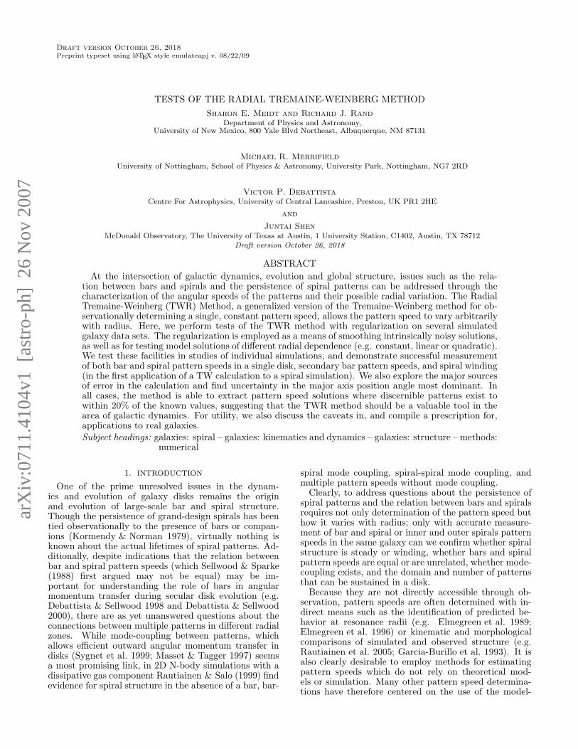
Fig. 1.— Illustration of a y>0 quadrature for a galaxy viewedfrom the negative z side with a tilt around the y axis by α=45.The horizontal lines, or slices, at positions yi are spaced at∆y=1.54, or ∆yobs=1.09, and represent integration between the

limits ±q

R2

0+ y2i where R0=10.8 is the maximum radial extent

of the quadrature. Each slice is carved into elements of width ∆rwhereby all the elements with the same shade of grey represent asingle radial bin rj .

slice i. In cases where multiple patterns exist in a singledisk, then, it is equally favorable (and hopefully suffi-cient) to extend all integrals to the edge of the surfacebrightness distribution.Meeting the requirement of integral convergence in this

manner as applied to the TWR calculation determinesthe location of the last radial bin jmax associated withelements Kijmax

along each slice. For a given radial binwidth, with the requirement that jmax equals N we arepresented with the size ofK as well as the outermost sliceposition, since jmax must also equal imax. One shouldcheck to see that KNN , the last entry in K associatedwith the outermost slice, is associated with a fully con-verged

∫

Σxdx (which achieves convergence at least bythe map boundary).Since K is an upper triangular matrix, the Ωj can be

solved for via simple back-substitution. In this way, solu-tions are generated from the outermost to the innermostradius (from light gray to black in Figure 1) according to

Ωk =bi −

∑Nj>k KijΩj

Kkk(8)

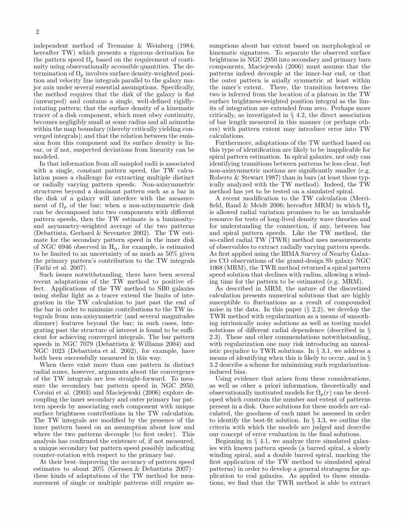
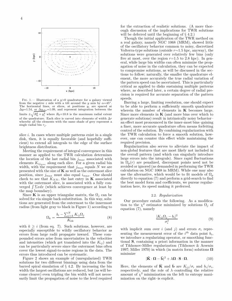
with k ≥ i (from eq. 7). Such solutions, however, areespecially susceptible to wildly oscillatory behavior aserrors from large radii propagate inward. These com-pounded errors arise from uncertainties in the velocitiesand intensities (which get translated into the Kij) andcan be particularly severe since the outermost bins oftencover the lowest signal-to-noise regions in the data. Theerrors thus introduced can be systematic.Figure 2 shows an example of (unregularized) TWR

solutions for two different binnings using data from thebarred spiral simulation of § 4.2. By increasing the binwidth the largest oscillations are reduced, but (as will be-come clearer) even tripling the bin width will not neces-sarily limit the propagation of noise to the level required

for the extraction of realistic solutions. (A more thor-ough discussion of the implications for TWR solutionswill be deferred until the beginning of § 4.2.)Though the initial application of the TWR method on

a real galaxy, namely NGC 1068 (MRM), showed littleof the oscillatory behavior common to noisy, discretizedVolterra-type solutions (outside r∼1.5 kpc, anyway), thesolutions were generated over relatively few bins (onlyfive at most, over the region r=1.5 to 2.8 kpc). In gen-eral, while large bin widths can often minimize the prop-agation of noise in the calculation, they can be expectedto compromise solutions, as will be discussed in the sec-tions to follow; naturally, the smaller the quadrature el-ement, the more accurately the true radial variation ofthe pattern speed can be ascertained. This is particularlycritical as applied to disks sustaining multiple patternswhere, as described later, a certain degree of radial pre-cision is required for accurate separation of the patternspeeds.Barring a large, limiting resolution, one should expect

to be able to perform a sufficiently smooth quadraturewherein the number of elements in K becomes large.Since more elements in K (and more bins over which togenerate solutions) result in intrinsically noisy behavior–an effect most pronounced in the inner-most bins–gaininga finer, more accurate quadrature often means forfeitingcontrol of the solution. By combining regularization withthe TWR calculation to force a smooth solution, how-ever, one can counter this effect while maintaining therequired precision.Regularization also serves to alleviate the impact of

non-global features that are most likely not included inthe overall pattern (and which can singularly introducelarge errors into the integrals). Since rapid fluctuationsin Ωp(r) are penalized, discrepant points need not beavoided or ignored (as demanded in performing the TWRcalculation on NGC 1068 in MRM). While one may alsouse the alternative, which would be to fit models of Ωp

directly to equation (7) and perform a grid-search to findthe best model form and coefficients, we pursue regular-ization here, its speed making it preferred.

2.2. Regularization

Our procedure entails the following. As a modifica-tion to the χ2 estimator minimized by solutions Ωj ofequation (7), namely

|KijΩj − bi|2

σ2i

(9)

with implicit sum over i (and j) and errors σi repre-senting the measurement error of the ith data point bi,we introduce a regularizing operator, or smoothing func-tional S, containing a priori information in the mannerof Tikhonov-Miller regularization (Tikhonov & Arsenin1997; Miller 1970) in which (in matrix form) solutions Ωminimize

|K ·Ω− b|2 + λΩ · S ·Ω. (10)

Here, the elements of K and b are Kij/σi and bi/σi,respectively, and the role of λ–controlling the relativeamount of χ2 minimization on the left to entropy maxi-mization on the right–is explicit.

5

Fig. 2.— Plots of (unregularized) TWR solutions for two different binnings of data from the barred spiral simulation in § 4.2 withSA=-45 (see § 4.1 for orientation convention). The left (right) panel shows the solution generated using ∆r=0.3 (0.9) bins.

Reduced to a linear set of normal equations, this mini-mization returns smoothed solutions according to a mod-ified version of equation (7):

(KT · K+ λS) ·Ω = KT · b (11)

Note that the regularizing functional, not necessarily up-per triangular, introduces an anticipatory quality to solu-tions Ωj whereby all bins at the same radius are coupled.Furthermore, solving for components Ωj no longer onlyinvolves a procedure like back-substitution, but requiresrather an L-U decomposition (for instance) as well.

2.3. The Smoothing Operator

The real power in applying regularization to TWR cal-culations is in the freedom to choose how the smooth-ness of solutions is achieved. For the purposes of distin-guishing between different possible radial dependencesfor Ω(r), we choose S to reflect a priori assumptionsbased on simple expectations from theory and observa-tion. Model solutions, then, each incorporating its ownS, represent smoothed, testable realizations of the pat-tern speed. These we restrict to simple forms in orderto minimize the additional amount of information to beextracted from the data relative to the traditional TWmethod.For polynomial solutions, we consider only constant,

linear and quadratic radial dependence. The elements ofthe smoothing S are associated with the minimization ofthe nth derivative of Ω(r) for each polynomial solutionof order n. For instance, for linear solutions this entailsminimizing

Ω · S ·Ω =

N−2∑

n=1

| − Ωn + 2Ωn+1 − Ωn+2|2 (12)

whereupon

S =

1 −2 1 0 0 0 0 . . . 0−2 5 −4 1 0 0 0 . . . 01 −4 6 −4 1 0 0 . . . 0...

. . ....

0 . . . 0 1 −4 6 −4 1 00 . . . 0 0 1 −4 6 −4 10 . . . 0 0 0 1 −4 5 −20 . . . 0 0 0 0 1 −2 1

. (13)

One may also choose a form for S that identifies twoor more distinct regions of independent radial behaviorby invoking a step-function model. For the case of abarred spiral with a constant bar and quadratic spiral,for instance, this corresponds to minimizing

Ω·S·Ω =

t−1∑

n=1

|Ωn +Ωn+1|2 for n<t

N−3∑

n=t

| − Ωn + 3Ωn+1 − 3Ωn+2 +Ωn+3|2 for n≥t.

(14)The elements of S with n < t reflect the a priori assump-tion that the bar pattern speed is constant, while thosefor n > t associate a quadratically varying pattern speedwith the spiral. The index t, a free parameter, locatesthe radial bin where the transition between the two pat-terns occurs. Obviously, the number of available binsconstrains the order of the polynomial in a given radialzone.Once we have chosen S, we initially choose λ to reflect

comparable amounts of χ2 minimization and regulariza-

tion by letting λ = λ0 = Tr

KT· K

/T r S. Since

we are in the business of generating solutions based onparticular models, λ is modified to arrive at the regu-larization required to return solutions of a given type.This modification generally consists of an increase in λover λ0. Consider how the regularizing parameter λ reg-ulates the degree of smoothness of the solution to theweight placed on the data: with λ=0, equation (10) cor-responds to χ2 minimization (and becomes an unbiasedestimator with the smallest variance), however yieldinghighly oscillatory solutions, while λ→∞ corresponds toa maximally smooth estimator with non-vanishing vari-ance.Fitting data sets with different spatial coverage will

change the effect of λ on the solution (e.g. larger binsrequire less regularization). The most appropriate choicefor λ (and S) should be made on a galaxy-by-galaxybasis, according to the quality of information to be ex-tracted from observations.

3. OTHER CONSIDERATIONS

6

3.1. Regularization-induced Bias

By imposing assumptions about the smoothness of thepattern speed, regularization inevitably introduces com-plications for extracting realistic solutions. To under-stand how these arise, consider the solution for a barredspiral galaxy. The nature of the calculation (from out toin) has implications for the accuracy of the bar estimates,in particular. Not only do the Ωj for bins covering thebar rely on the greatest number of matrix elements (anderrors therein), but the bar estimate depends critically onthe solution for the spiral and all outer bins via equation(8). Consequently, merely requiring the pattern speed inthe outer bins to be constant with regularization out tothe edge of the surface density (for instance)–effectivelyremoving fluctuations that might better fit the data–willhave consequences for the bar solutions. So while theregularization is particularly fast and effective for testsfor the radial behavior of patterns, it can also hinder therealization of accurate solutions.For the simulations studied here, the risk of

regularization-induced bias is inherited from the adoptedquadrature. Recall our requirement that all slices coverthe full extent of the ‘emission’–so as to insure all inte-grals be fully converged–and relatedly, that the last ma-trix element governs the outermost slice position. In thebarred spiral simulation of § 4.2, for example, such anextensive quadrature presents us with outermost slicesthat pass through a region where there is simply no dis-cernible pattern (as indicated by the surface brightnessdistribution and its Fourier decomposition; see next sec-tion). While these slices themselves do not provide directestimates of the patterns of interest, the correspondingbin values are necessary for calculating the bar and spiralsolutions. Moreover, the quality of these solutions willbe intimately related to the treatment of the outermostbins. We therefore find that identifying, and reducingthe influence of, the compromised zone by not enforcingregularization on these bins to be essential for accuratepattern speed measurement.

3.2. Fourier Diagnostics

With the above concerns in mind, we have tested andused the following scheme. Given slices that pass throughan outer region which either contains little informationfrom a strong pattern, is suspected of sustaining multi-ple patterns, or displays only faint emission, we choosein such a case to let the values in the outermost binsbe calculated without regularization with the restriction,only, that they minimize the χ2. Once a particular bin–at rc, the cut radius–has been reached, regularization isimposed with all remaining inward bins generated ac-cordingly.In our procedure this corresponds to using an S in-

dexed by the cut bin c that is lowest-block zero. Andthe ‘cut’ radius identifies the location in the disk wherethe outermost discernible pattern ends. Note that thisis in contrast to altogether ignoring the outer portion ofthe disk. We prefer this procedure for two reasons: 1) asqualified later in § 4.2.2, when each integral is truncatedwithin the disk, the quadrature is at greater risk of ig-noring information critical for characterizing the patternsuniformly throughout the disk and 2) like the transitionradius rt, we can easily incorporate rc as a free, though

restricted, parameter in our models.In practice, extracting the bar and spiral pattern

speeds for the simulated barred spiral in § 4.2 involvesgenerating a group of solutions with various bar-to-spiral pattern transition radii for a given ‘cut’ location.Throughout the analysis, we choose the cut radius toreflect a priori knowledge of the outermost measurablepattern’s termination radius estimated from the surfacebrightness and its Fourier decomposition. When referredto, the power in each Fourier component, or mode m, isgiven by the norm of the complex Fourier amplitude

Ii =

N∑

n=1

eimθn (15)

where θn is the angular coordinate of each of the N par-ticles at each measured radius.For the barred spiral in § 4.2, for example, we com-

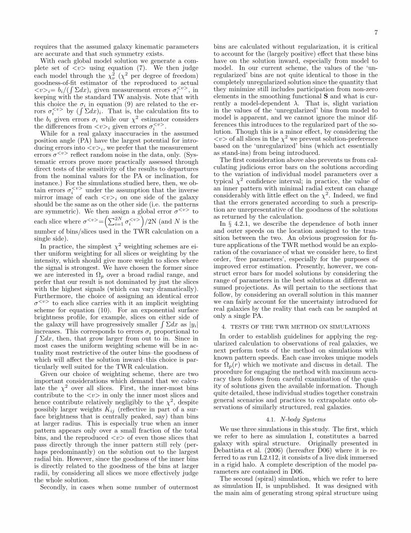
bine evidence from the surface density–where beyond thebar there is enhanced spiral surface density from only alimited radial zone–with the Fourier spectrum to iden-tify a region in the disk outside the spiral which is sus-ceptible to regularization-induced bias. Specifically, theFourier power spectrum (Figure 4) shows that at r∼5.0the second clean hump in m=2 power decreases to almostzero, marking the end of the spiral. Past this radius,the (strong) m=2 component (between r∼6.0-8.0) is notassociated with visible spiral structure (see Figure 3).Reckoning this outer zone to be incompatible with a sim-ple pattern speed model, then, we consider only the in-ward bar and primary spiral pattern speeds to be measur-able with regularization. Figure 19 of Debattista et al.(2006) for this simulation (Figure 5 in this paper) con-firms this; not only does the spiral pattern terminateat rc∼5.0, but beyond this radius the pattern speed ismulti-valued (this, of course, would be indiscernible in areal galaxy). In this case, imposing form with regular-ization on bins of suspect quality and behavior outsidethe spiral will likely impair the solution of interest. Wetherefore restrict the cut bin for the barred spiral simula-tion to 4.5<rc<6.0, representative of where the primaryspiral pattern terminates in the disk. As mentioned in§ 4.2, this step is substantiated by our finding that acut radius of rc=4.8 is one of several χ2 minima given arange of possible cut radii. And furthermore, solutionsgenerated in this manner are judged to overall provide aconsiderably better fit to the data than solutions whereregularization is imposed out to the edge of the surfacebrightness (according to the scheme described in the nextsection).

3.3. Weighting Schemes and Goodness-of-Fit

Given the data, we simultaneously generate model so-lutions with different radial dependences for direct com-parison for each side (y>0 or y<0) independently. Wethen average the two like-model solutions together toconstruct a global solution. (In those instances whenmodel solutions include a cut bin, the averaging occursover the regularized part of the solutions only, in orderto maintain the ‘unbiased’ quality of the unregularizedpart of the solutions for each side of the galaxy.) Notethat while the assumption that the patterns are indeedglobal is not overly inspired for the simulated galaxiesstudied here, putting this into practice on a real galaxy

7

requires that the assumed galaxy kinematic parametersare accurate and that such symmetry exists.With each global model solution we generate a com-

plete set of <v> using equation (7). We then judgeeach model through the χ2

ν (χ2 per degree of freedom)goodness-of-fit estimator of the reproduced to actual<v>i= bi/(

∫

Σdx)i given measurement errors σ<v>i , in

keeping with the standard TW analysis. Note that withthis choice the σi in equation (9) are related to the er-rors σ<v>

i by (∫

Σdx)i. That is, the calculation fits tothe bi given errors σi while our χ2 estimator considersthe differences from <v>i given errors σ<v>

i .While for a real galaxy inaccuracies in the assumed

position angle (PA) have the largest potential for intro-ducing errors into <v>i, we prefer that the measurementerrors σ<v> reflect random noise in the data, only. (Sys-tematic errors prove more practically assessed throughdirect tests of the sensitivity of the results to departuresfrom the nominal values for the PA or inclination, forinstance.) For the simulations studied here, then, we ob-tain errors σ<v>

i under the assumption that the inversemirror image of each <v>i on one side of the galaxyshould be the same as on the other side (i.e. the patternsare symmetric). We then assign a global error σ<v> to

each slice where σ<v>=(

∑2Ni=1 σ

<v>i

)

/2N (and N is the

number of bins/slices used in the TWR calculation on asingle side).In practice, the simplest χ2 weighting schemes are ei-

ther uniform weighting for all slices or weighting by theintensity, which should give more weight to slices wherethe signal is strongest. We have chosen the former sincewe are interested in Ωp over a broad radial range, andprefer that our result is not dominated by just the sliceswith the highest signals (which can vary dramatically).Furthermore, the choice of assigning an identical errorσ<v> to each slice carries with it an implicit weightingscheme for equation (10). For an exponential surfacebrightness profile, for example, slices on either side ofthe galaxy will have progressively smaller

∫

Σdx as |yi|increases. This corresponds to errors σi proportional to∫

Σdx, then, that grow larger from out to in. Since inmost cases the uniform weighting scheme will be in ac-tuality most restrictive of the outer bins–the goodness ofwhich will affect the solution inward–this choice is par-ticularly well suited for the TWR calculation.Given our choice of weighting scheme, there are two

important considerations which demand that we calcu-late the χ2 over all slices. First, the inner-most binscontribute to the <v> in only the inner most slices andhence contribute relatively negligibly to the χ2, despitepossibly larger weights Kij (reflective in part of a sur-face brightness that is centrally peaked, say) than binsat larger radius. This is especially true when an innerpattern appears only over a small fraction of the totalbins, and the reproduced <v> of even those slices thatpass directly through the inner pattern still rely (per-haps predominantly) on the solution out to the largestradial bin. However, since the goodness of the inner binsis directly related to the goodness of the bins at largerradii, by considering all slices we more effectively judgethe whole solution.Secondly, in cases when some number of outermost

bins are calculated without regularization, it is criticalto account for the (largely positive) effect that these binshave on the solution inward, especially from model tomodel. In our current scheme, the values of the ‘un-regularized’ bins are not quite identical to those in thecompletely unregularized solution since the quantity thatthey minimize still includes participation from non-zeroelements in the smoothing functional S and what is cur-rently a model-dependent λ. That is, slight variationin the values of the ‘unregularized’ bins from model tomodel is apparent, and we cannot ignore the minor dif-ferences this introduces to the regularized part of the so-lution. Though this is a minor effect, by considering the<v> of all slices in the χ2 we prevent solution-preferencebased on the ‘unregularized’ bins (which act essentiallyas stand-ins) from being introduced.The first consideration above also prevents us from cal-

culating judicious error bars on the solutions accordingto the variation of individual model parameters over atypical χ2 confidence interval; in practice, the value ofan inner pattern with minimal radial extent can changeconsiderably with little effect on the χ2. Indeed, we findthat the errors generated according to such a prescrip-tion are unrepresentative of the goodness of the solutionsas returned by the calculation.In § 4.2.1, we describe the dependence of both inner

and outer speeds on the location assigned to the tran-sition between the two. An obvious progression for fu-ture applications of the TWR method would be an explo-ration of the covariance of what we consider here, to firstorder, ‘free parameters’, especially for the purposes ofimproved error estimation. Presently, however, we con-struct error bars for model solutions by considering therange of parameters in the best solutions at different as-sumed projections. As will pertain to the sections thatfollow, by considering an overall solution in this mannerwe can fairly account for the uncertainty introduced forreal galaxies by the reality that each can be sampled atonly a single PA.

4. TESTS OF THE TWR METHOD ON SIMULATIONS

In order to establish guidelines for applying the reg-ularized calculation to observations of real galaxies, wenext perform tests of the method on simulations withknown pattern speeds. Each case invokes unique modelsfor Ωp(r) which we motivate and discuss in detail. Theprocedure for engaging the method with maximum accu-racy then follows from careful examination of the qual-ity of solutions given the available information. Thoughquite detailed, these individual studies together constraingeneral scenarios and practices to extrapolate onto ob-servations of similarly structured, real galaxies.

4.1. N-body Systems

We use three simulations in this study. The first, whichwe refer to here as simulation I, constitutes a barredgalaxy with spiral structure. Originally presented inDebattista et al. (2006) (hereafter D06) where it is re-ferred to as run L2.t12, it consists of a live disk immersedin a rigid halo. A complete description of the model pa-rameters are contained in D06.The second (spiral) simulation, which we refer to here

as simulation II, is unpublished. It was designed withthe main aim of generating strong spiral structure using

8

the groove mode mechanism of Sellwood & Lin (1989)and Sellwood & Kahn (1991) in which dynamical insta-bility develops from a ’groove’, or narrow feature, in thephase-space density at a particular angular momentum.A trailing spiral wave is generated, and at the LindbladResonances of the wave, further grooves develop suchthat the instability is recurrent. Like simulation I, itconsists of a rigid halo and live disk, but also includes alive bulge component. The bulge constitutes 25% of thebaryonic mass and is sufficiently concentrated that a baris very slow in forming. The disk has Toomre-Q = 1.2; inorder that a strong spiral was seeded, ∼ 6% of disk parti-cles in a narrow angular momentum range were removedleaving 4×106-169480 particles including the bulge. Theresult, as can be seen in Figure 11, is the formation of astrong but transient spiral.The last simulation in this paper, simulation III, is

a double-barred galaxy generated using the method ofDebattista & Shen (2007). This high-resolution simula-tion consists of live disk and bulge components in a rigidhalo potential. The model has ∼ 4.8 million equal massparticles, with ∼ 4 million in the disk and ∼ 0.8 millionin the bulge such that the bulge has mass Mb = 0.2Md,where Md is the disk mass. The initial Toomre-Q ofthe disk is ≃ 2. The formation of the secondary bar isinduced by making the bulge rotate (to mimic a pseu-dobulge). More details of the simulation can be found inShen & Debattista (2007) where it is referred to as runD.As in D06, all lengths and velocities are here presented

in natural units. We analyze a snapshot of each simula-tion at a single time step with the disk in the xy plane.By rotating the system about the z axis we assign a line-of-sight direction to establish the kinematical major axis.Another rotation about the x axis gives the system aninclination α (chosen throughout at α=45, unless other-wise specified). The snapshot is then projected onto thesky-plane where xobs=x and yobs=y cosα. For a givenslice spacing, the slices along which the calculations oc-cur are aligned perpendicular to the line-of-sight direc-tion (parallel to the kinematical major axis). The orien-tation of these slices, which is identical to the disk PA ina real observation, is designated uniquely the slice angle(SA) in the studies that follow.

4.2. Simulation I: Barred Spiral Galaxy

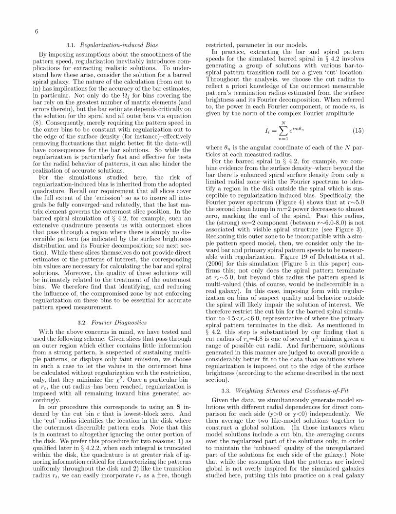
The bar and spiral structure in this simulation, firstpresented in D06, is featured out to r∼5.0, clear in thesurface density (Figure 3) and its Fourier decomposition(Figure 4). Beyond r∼5.0, the Fourier decompositionindicates the possible presence of a third pattern. Withstep-models for Ωp(r), then, we might reasonably extractpattern speeds for three distinct structures. However, them=2 mode between 5.0<r<8.0 is not associated with astrong surface density enhancement. And as remarkedupon in § 3.2, Figure 19 in D06 reproduced here in Figure5 shows that the pattern in this radial zone is maintainedby multiple distinct pattern speeds. (Note that a realgalaxy would not be disposed to the analysis providedwith this type of plot. It is available for this simulation,only, and we include it here for the sake of compari-son). In a clear account of regularization-induced bias,test solutions based on a three-pattern speed model haveconsiderably larger χ2 than those parameterizing a bar

Fig. 3.— Face-on display of the barred spiral simulation’s surfacebrightness distribution projected with a -30 rotation about the zaxis. For reference, the alignment of the TWR quadrature for aframe at this orientation is designated SA=+60.

Fig. 4.— Fourier power spectrum of the barred spiral simulation’ssurface brightness distribution shown in Figure 3. Modes up tom = 4 are plotted as a function of radius with lines for m = 1 indot, m = 2 in solid, m = 3 in dash-dot-dot, and m = 4 in dash.

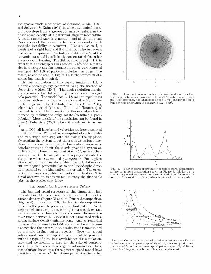
Fig. 5.— Contours of the barred spiral simulation’s m=2 Fouriermode showing a bar pattern speed Ωb=0.29, a bar-to-spiral transi-tion of rt∼2.5, and a dominant spiral pattern speed Ωs=0.18 outto r∼4.5-5.5 beyond which multiple spiral modes exist.

9

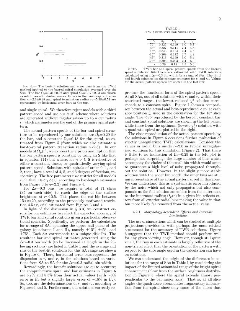
Fig. 6.— The best-fit solution and error bars from the TWRmethod applied to the barred spiral simulation averaged over sixSAs. The bar Ωb=0.31±0.02 and spiral Ωs=0.17±0.03 are shownas solid lines with dashed errors. Errors in the bar-to-spiral transi-tion rt=2.6±0.28 and spiral termination radius rc=5.38±0.54 arerepresented by horizontal error bars at the top.

and single spiral. We therefore reject models with a thirdpattern speed and use our ‘cut’ scheme where solutionsare generated without regularization up to a cut radiusrc which parameterizes the end of the primary spiral pat-tern.The actual pattern speeds of the bar and spiral struc-

ture to be reproduced by our solutions are Ωb=0.29 forthe bar, and a constant Ωs=0.18 for the spiral, as es-timated from Figure 5 (from which we also estimate abar-to-spiral pattern transition radius r∼2.5). In ourmodels of Ωp(r), we express the a priori assumption thatthe bar pattern speed is constant by using an S like thatin equation (14) but where, for n > t, S is reflective ofeither a constant, linear, or quadratically varying spiralpattern speed. Solutions with spirals of order 0, 1, and2, then, have a total of 4, 5, and 6 degrees of freedom, re-spectively. The free parameter t we restrict for all modelssuch that 1.8<rt<3.0, according to bar-length estimatesfrom Figure 3 (aB∼2.2) and Figure 4.For ∆r=0.3 bins, we require a total of 71 slices

(35 on each side) to reach the edge of the surfacebrightness at r∼10.5. This places the cut bin between15<c<20, according to the previously motivated restric-tion 4.5<rc<6.0 estimated from Figures 3 and 4.In light of the discussion in § 3.3, we construct er-

rors for our estimates to reflect the expected accuracy ofTWR bar and spiral solutions given a particular observa-tional scenario. Specifically, we perform the calculationfor a range of SAs spanning the upper half-plane of thegalaxy (quadrants I and II), namely ±15, ±45, and±75. Each SA corresponds to a unique disk PA. Theresultant bar and spiral estimates generated using the∆r=0.3 bin width (to be discussed at length in the fol-lowing sections) are listed in Table 1 and the average andrms of the best-fit solutions for this SA range are shownin Figure 6. There, horizontal error bars represent thedispersion in rt and rc in the solutions based on varia-tions from SA to SA for the ∆r=0.3 radial bin width.Rewardingly, the best-fit solutions are quite accurate;

the comprehensive spiral and bar estimates in Figure 6are 6.7% and 8.3% from their actual values (with ∼8%error in Ωb but a slightly larger error of ∼18% in Ωs).So, too, are the determinations of rt and rc, according toFigures 4 and 5. Furthermore, our solutions correctly re-

TABLE 1TWR estimates for Simulation I.

SA Ωb Ωs rt rc75 0.325 0.149 3.0 5.745 0.327 0.111 2.4 4.815 0.343 0.184 2.4 4.5-15 0.269 0.172 2.7 4.8-45 0.313 0.199 3.0 5.4-75 0.303 0.203 2.4 6.0

- 0.29 0.18 2.5 5.0

Note. — TWR bar and spiral pattern speeds from the barredspiral simulation listed here are estimated with TWR solutionscalculated using a ∆r=0.3 bin width for a range of SAs. The thirdand fourth columns list the connate estimates for rt and rc. Valuesfor the actual pattern speeds are shown in the last row.

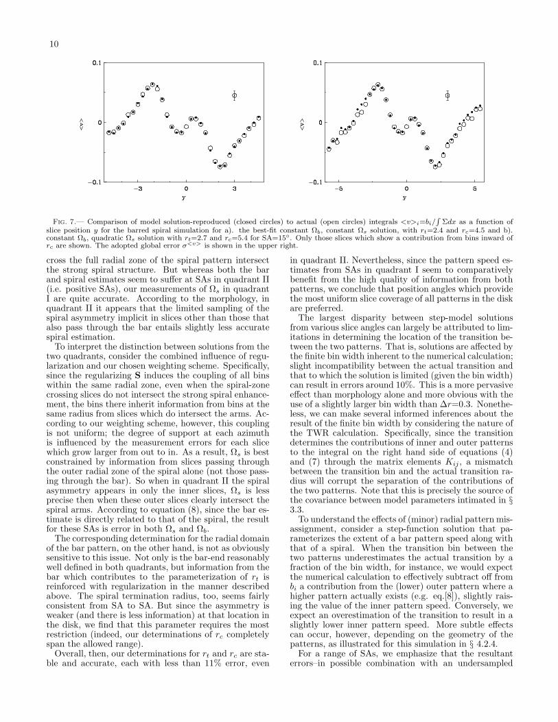
produce the functional form of the spiral pattern speed.At all SAs, out of all solutions with rt and rc within theirrestricted ranges, the lowest reduced χ2 solution corre-sponds to a constant spiral. Figure 7 shows a compari-son between the actual and best-reproduced<v> at eachslice position yi used in the calculation for the 15 sliceangle. The <v> reproduced by the best-fit constant barand constant spiral solutions are shown in the left panel,while those from the optimum (lowest-χ2

ν) solution witha quadratic spiral are plotted in the right.The close reproduction of the actual pattern speeds by

the solutions in Figure 6 occasions further evaluation ofstrictly unregularized TWR calculations. Consider thevalues in radial bins inside r∼2.0 in typical unregular-ized solutions for this simulation (Figure 2). That thereis little to no indication of Ωb=0.29 in the left plot isperhaps not surprising: the large number of bins whichaccompany the choice of the small bin width would seemto guarantee a high level of noise propagated through-out the solution. However, in the slightly more stablesolution with the wider bin width, the inner bins are stillunrepresentative of the actual pattern speed in this zone.We can understand this as a systematic error introducedby the noise which not only propagates but also com-pounds as the full solution assembles from the outermostto the innermost radius; Ωp(r) in a given bin reflects er-rors from all exterior radial bins making the value in thatbin more likely far removed from the actual value.

4.2.1. Morphology-dependent Effects and IntrinsicLimitations

The use of simulations which can be studied at multipleprojections provides us with perhaps the most criticalassessment for the accuracy of TWR solutions. Figure6 suggests that the TWR method should perform wellfor any given viewing angle. However, though still quitesmall, the rms in each estimate is largely reflective of thenon-trivial effect that the orientation of the pattern withrespect to the slice angle used in the calculation can haveon solutions.We can understand the origin of the differences in so-

lutions for the range of SAs in Table 1 by considering theimpact of the limited azimuthal range of the bright spiralenhancement (clear from the surface brightness distribu-tion in Figure 3 where the spiral extends almost per-pendicular to the bar major axis). That is, at all sliceangles the quadrature accumulates fragmentary informa-tion from the spiral since only some of the slices that

10

Fig. 7.— Comparison of model solution-reproduced (closed circles) to actual (open circles) integrals <v>i=bi/R

Σdx as a function ofslice position y for the barred spiral simulation for a). the best-fit constant Ωb, constant Ωs solution, with rt=2.4 and rc=4.5 and b).constant Ωb, quadratic Ωs solution with rt=2.7 and rc=5.4 for SA=15. Only those slices which show a contribution from bins inward ofrc are shown. The adopted global error σ<v> is shown in the upper right.

cross the full radial zone of the spiral pattern intersectthe strong spiral structure. But whereas both the barand spiral estimates seem to suffer at SAs in quadrant II(i.e. positive SAs), our measurements of Ωs in quadrantI are quite accurate. According to the morphology, inquadrant II it appears that the limited sampling of thespiral asymmetry implicit in slices other than those thatalso pass through the bar entails slightly less accuratespiral estimation.To interpret the distinction between solutions from the

two quadrants, consider the combined influence of regu-larization and our chosen weighting scheme. Specifically,since the regularizing S induces the coupling of all binswithin the same radial zone, even when the spiral-zonecrossing slices do not intersect the strong spiral enhance-ment, the bins there inherit information from bins at thesame radius from slices which do intersect the arms. Ac-cording to our weighting scheme, however, this couplingis not uniform; the degree of support at each azimuthis influenced by the measurement errors for each slicewhich grow larger from out to in. As a result, Ωs is bestconstrained by information from slices passing throughthe outer radial zone of the spiral alone (not those pass-ing through the bar). So when in quadrant II the spiralasymmetry appears in only the inner slices, Ωs is lessprecise then when these outer slices clearly intersect thespiral arms. According to equation (8), since the bar es-timate is directly related to that of the spiral, the resultfor these SAs is error in both Ωs and Ωb.The corresponding determination for the radial domain

of the bar pattern, on the other hand, is not as obviouslysensitive to this issue. Not only is the bar-end reasonablywell defined in both quadrants, but information from thebar which contributes to the parameterization of rt isreinforced with regularization in the manner describedabove. The spiral termination radius, too, seems fairlyconsistent from SA to SA. But since the asymmetry isweaker (and there is less information) at that location inthe disk, we find that this parameter requires the mostrestriction (indeed, our determinations of rc completelyspan the allowed range).Overall, then, our determinations for rt and rc are sta-

ble and accurate, each with less than 11% error, even

in quadrant II. Nevertheless, since the pattern speed es-timates from SAs in quadrant I seem to comparativelybenefit from the high quality of information from bothpatterns, we conclude that position angles which providethe most uniform slice coverage of all patterns in the diskare preferred.The largest disparity between step-model solutions

from various slice angles can largely be attributed to lim-itations in determining the location of the transition be-tween the two patterns. That is, solutions are affected bythe finite bin width inherent to the numerical calculation;slight incompatibility between the actual transition andthat to which the solution is limited (given the bin width)can result in errors around 10%. This is a more pervasiveeffect than morphology alone and more obvious with theuse of a slightly larger bin width than ∆r=0.3. Nonethe-less, we can make several informed inferences about theresult of the finite bin width by considering the nature ofthe TWR calculation. Specifically, since the transitiondetermines the contributions of inner and outer patternsto the integral on the right hand side of equations (4)and (7) through the matrix elements Kij , a mismatchbetween the transition bin and the actual transition ra-dius will corrupt the separation of the contributions ofthe two patterns. Note that this is precisely the source ofthe covariance between model parameters intimated in §3.3.To understand the effects of (minor) radial pattern mis-

assignment, consider a step-function solution that pa-rameterizes the extent of a bar pattern speed along withthat of a spiral. When the transition bin between thetwo patterns underestimates the actual transition by afraction of the bin width, for instance, we would expectthe numerical calculation to effectively subtract off frombi a contribution from the (lower) outer pattern where ahigher pattern actually exists (e.g. eq.[8]), slightly rais-ing the value of the inner pattern speed. Conversely, weexpect an overestimation of the transition to result in aslightly lower inner pattern speed. More subtle effectscan occur, however, depending on the geometry of thepatterns, as illustrated for this simulation in § 4.2.4.For a range of SAs, we emphasize that the resultant

errors–in possible combination with an undersampled

11

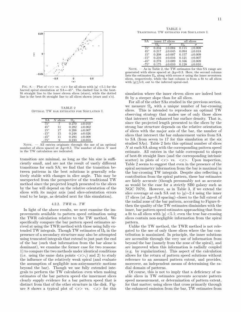
Fig. 8.— Plot of <v> vs. <x> for all slices with |y| <5.1 for thebarred spiral simulation at SA=-45. The dashed line is the best-fit straight line to the inner eleven slices (stars), while the dottedline is the best-fit straight line to all slices shown (stars and x’s).

TABLE 2Optimal TW bar estimates for Simulation I.

SA N slices Ωp σ75 7 0.270 ±0.01045 11 0.282 ±0.06215 17 0.208 ±0.007-15 15 0.248 ±0.026-45 11 0.294 ±0.008-75 9 0.233 ±0.053

Note. — All entries originate through the use of an optimalnumber of slices spaced at ∆y=0.3. The number of slices N usedin the TW calculation are indicated.

transition–are minimal, as long as the bin size is suffi-ciently small, and are not the result of vastly differenttransitions for each SA; we find that the transition be-tween patterns in the best solutions is generally rela-tively stable with changes in slice angle. This may beunexpected from the perspective of the traditional TWmethod since the projected length presented to the slicesby the bar will depend on the relative orientation of theslices with its major axis (and slice-orientation errorstend to be large, as detailed next for this simulation).

4.2.2. TWR vs. TW

In light of the above results, we next examine the im-provements available to pattern speed estimation usingthe TWR calculation relative to the TW method. Wespecifically compare the bar pattern speed estimates ar-rived at using the TWRmethod with those using fully ex-tended TW integrals. Though TW estimates of Ωb in thepresence of a secondary structure may also be attemptedusing truncated integrals that extend to just past the endof the bar (such that information from the bar alone isdominant), we examine the former case for two reasons:1) to compare the two methods under identical conditions(i.e. using the same data points <v>i) and 2) to studythe influence of the relatively weak spiral (and evaluatethe assumption of negligible non-axisymmetric motionsbeyond the bar). Though we use fully extended inte-grals to perform the TW calculation–even when makingestimates of the bar pattern speed–the innermost slicesclearly supply evidence for a bar pattern speed that isdistinct from that of the other structure in the disk. Fig-ure 8 shows a typical plot of <v> vs. <x> for this

TABLE 3Traditional TW estimates for Simulation I.

SA inner 17 slices all slicesΩp σ Ωp σ

75 0.234 ±0.004 0.115 ±0.00845 0.217 ±0.045 0.094 ±0.01815 0.208 ±0.007 0.157 ±0.009-15 0.216 ±0.016 0.121 ±0.007-45 0.278 ±0.009 0.166 ±0.009-75 0.175 ±0.010 0.128 ±0.010

Note. — As in Table 2, the TW estimates for this SA range aregenerated with slices spaced at ∆y=0.3. Here, the second columnlists the estimates Ωp along with errors σ using the inner seventeenslices, respectively, while the last column is from a fit to all sliceswith |y|≤5.0, out to the inferred spiral-end.

simulation where the inner eleven slices are indeed bestfit by a steeper slope than for all slices.For all of the other SAs studied in the previous section,

we measure Ωp with a unique number of bar-crossingslices. This is intended to reproduce an optimal TWobserving strategy that makes use of only those slicesthat intersect the enhanced bar surface density. That is,since the projected length presented to the slices by thestrong bar structure depends on the relative orientationof slices with the major axis of the bar, the number ofslices that intersect the bar enhancement varies from SAto SA (from seven to 17 for this simulation at the sixstudied SAs). Table 2 lists this optimal number of slicesN at each SA along with the corresponding pattern speedestimate. All entries in the table correspond to slopesof best-fit straight lines (and the corresponding intrinsicscatter) in plots of <v> vs. <x>. Upon inspection,Table 2 seems to suggest that even in the presence of thespiral asymmetry information from the bar is maximal inthe bar-crossing TW integrals. Despite also reflecting acontribution from the spiral pattern, these bar estimatesare fairly accurate (though presumably not as accurateas would be the case for a strictly SB0 galaxy such asNGC 7079). However, as in Table 3, if we extend theslice coverage at each SA out to |y|∼2.4 using the inner17 slices (at ∆y=0.3 spacing)–closer to the full extent ofthe radial zone of the bar pattern, according to Figure 6–then the quality of the TW estimates diminishes with theinner, bar pattern speed estimates approaching that froma fit to all slices with |y| <5.1; even the true bar-crossingslices contain non-negligible information from the spiralpattern.Unlike the TW method, the TWR method is not rele-

gated to the use of only those slices where the bar con-tribution is maximized. In principle, the inner solutionsare accessible through the very use of information frombeyond the bar (namely from the zone of the spiral), andare improved when this information is radially coupled(e.g. by regularization). This aspect of the calculationallows for the return of pattern speed solutions withoutreference to an assumed pattern extent, and provides,moreover, an independent means of determining the ra-dial domain of patterns.Of course, this is not to imply that a deficiency of us-

able slices in TW estimates prevents accurate patternspeed measurement, or determination of pattern extent,for that matter; using slices that cross primarily throughthe enhanced emission from the bar, TW estimates from

12

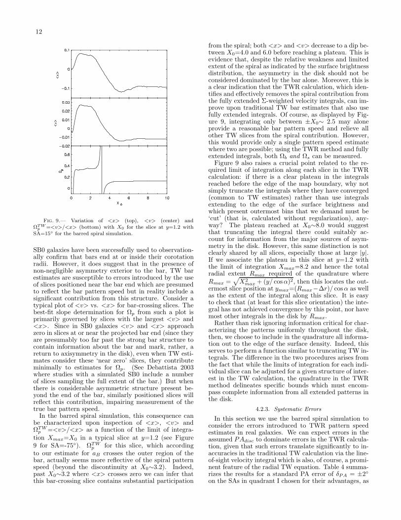
Fig. 9.— Variation of <x> (top), <v> (center) andΩTW

p =<v>/<x> (bottom) with X0 for the slice at y=1.2 withSA=15 for the barred spiral simulation.

SB0 galaxies have been successfully used to observation-ally confirm that bars end at or inside their corotationradii. However, it does suggest that in the presence ofnon-negligible asymmetry exterior to the bar, TW barestimates are susceptible to errors introduced by the useof slices positioned near the bar end which are presumedto reflect the bar pattern speed but in reality include asignificant contribution from this structure. Consider atypical plot of <v> vs. <x> for bar-crossing slices. Thebest-fit slope determination for Ωp from such a plot isprimarily governed by slices with the largest <v> and<x>. Since in SB0 galaxies <v> and <x> approachzero in slices at or near the projected bar end (since theyare presumably too far past the strong bar structure tocontain information about the bar and mark, rather, areturn to axisymmetry in the disk), even when TW esti-mates consider these ‘near zero’ slices, they contributeminimally to estimates for Ωp. (See Debattista 2003where studies with a simulated SB0 include a numberof slices sampling the full extent of the bar.) But whenthere is considerable asymmetric structure present be-yond the end of the bar, similarly positioned slices willreflect this contribution, impairing measurement of thetrue bar pattern speed.In the barred spiral simulation, this consequence can

be characterized upon inspection of <x>, <v> andΩTW

p =<v>/<x> as a function of the limit of integra-tion Xmax=X0 in a typical slice at y=1.2 (see Figure9 for SA=-75). ΩTW

p for this slice, which accordingto our estimate for aB crosses the outer region of thebar, actually seems more reflective of the spiral patternspeed (beyond the discontinuity at X0∼3.2). Indeed,past X0∼3.2 where <x> crosses zero we can infer thatthis bar-crossing slice contains substantial participation

from the spiral; both <x> and <v> decrease to a dip be-tween X0=4.0 and 6.0 before reaching a plateau. This isevidence that, despite the relative weakness and limitedextent of the spiral as indicated by the surface brightnessdistribution, the asymmetry in the disk should not beconsidered dominated by the bar alone. Moreover, this isa clear indication that the TWR calculation, which iden-tifies and effectively removes the spiral contribution fromthe fully extended Σ-weighted velocity integrals, can im-prove upon traditional TW bar estimates that also usefully extended integrals. Of course, as displayed by Fig-ure 9, integrating only between ±X0∼ 2.5 may aloneprovide a reasonable bar pattern speed and relieve allother TW slices from the spiral contribution. However,this would provide only a single pattern speed estimatewhere two are possible; using the TWR method and fullyextended integrals, both Ωb and Ωs can be measured.Figure 9 also raises a crucial point related to the re-

quired limit of integration along each slice in the TWRcalculation: if there is a clear plateau in the integralsreached before the edge of the map boundary, why notsimply truncate the integrals where they have converged(common to TW estimates) rather than use integralsextending to the edge of the surface brightness andwhich present outermost bins that we demand must be‘cut’ (that is, calculated without regularization), any-way? The plateau reached at X0∼8.0 would suggestthat truncating the integral there could suitably ac-count for information from the major sources of asym-metry in the disk. However, this same distinction is notclearly shared by all slices, especially those at large |y|.If we associate the plateau in this slice at y=1.2 withthe limit of integration Xmax=8.2 and hence the totalradial extent Rmax required of the quadrature whereRmax =

√

X2max + (y/ cosα)2, then this locates the out-

ermost slice position at ymax=(Rmax−∆r)/ cosα as wellas the extent of the integral along this slice. It is easyto check that (at least for this slice orientation) the inte-gral has not achieved convergence by this point, nor havemost other integrals in the disk by Rmax.Rather than risk ignoring information critical for char-

acterizing the patterns uniformly throughout the disk,then, we choose to include in the quadrature all informa-tion out to the edge of the surface density. Indeed, thisserves to perform a function similar to truncating TW in-tegrals. The difference in the two procedures arises fromthe fact that while the limits of integration for each indi-vidual slice can be adjusted for a given structure of inter-est in the TW calculation, the quadrature in the TWRmethod delineates specific bounds which must encom-pass complete information from all extended patterns inthe disk.

4.2.3. Systematic Errors

In this section we use the barred spiral simulation toconsider the errors introduced to TWR pattern speedestimates in real galaxies. We can expect errors in theassumed PAdisc to dominate errors in the TWR calcula-tion, given that such errors translate significantly to in-accuracies in the traditional TW calculation via the line-of-sight velocity integral which is also, of course, a promi-nent feature of the radial TW equation. Table 4 summa-rizes the results for a standard PA error of δPA = ±2

on the SAs in quadrant I chosen for their advantages, as

13

TABLE 4PA errors in TW and TWR estimates for Simulation I.

δPA = +2 δPA = −2

Ωb Ωs Ωb Ωs

TW* 0.179 0.162 0.354 0.115±0.055 ±0.058 ±0.04 ±0.02

TWR 0.214 0.211 0.380 0.158±0.031 ±0.045 ±0.042 ±0.023

Note. — Entries correspond to average bar and spiral estimatesfrom SAs in quadrant I (-15,-45, and -75) with PA errors δPA =+2 and −2. Estimates from both the traditional TW (*barestimates using the nominal number of slices for each SA listedin Table 2 and TWR methods are listed).

evidenced by the discussion in § 4.2.1. The average andrms for bar and spiral estimates from both the TWR andthe traditional TW methods are listed. (The TW ‘bar’estimates are obtained by fitting to the inner, nominalnumber of slices listed in Table 2, while all slices with|y|<5.1 are considered in the ‘spiral’ estimates.)Even this small δPA introduces considerable errors (rel-

ative to the known pattern speeds) to both types of barestimates. These errors in Ωb can be many times largerthan the formal rms. But whereas the errors are com-parable in the TWR and TW bar estimates, the errorsin the spiral estimates tend to be smaller with TWRthan TW. Rewardingly, with this error not only are theTWR spiral solutions still definitively constant and ac-curate to ∼15%, but the radial domain of both patternspeeds are still well-determined. The transition betweenthe bar and spiral rt and the termination radius of thestrong spiral pattern rc are effectively unchanged fromthe δPA = 0 case; for both δPA = +2 and δPA = −2

we find rt=2.8±0.37and rc=5.4±0.46.Besides the effects on PAdisc measurement as studied

by Debattista (2003), galaxy inclination and ellipticityplay perhaps more prominent roles as sources of errorin TWR solutions relative to traditional TW estimates.Presumably, large inclination errors will prevent the as-sociation of information into accurate radial bins, giventhat r = yobs/ cosα. We expect this effect to be minimalat moderate inclinations since dr ∝ dα sinα, and mostsignificant at small inclinations where one would gener-ally find that the difficulty in inferring in-plane morphol-ogy and kinematics makes the the TW method imprac-tical in any case. At a moderate, 45 inclination we findthat the barred spiral solutions for ± 3 inclination errordiffer from the actual pattern speeds by only the changein sinα introduced by the line-of-sight velocity.

4.2.4. Transition Mis-identification

We have shown that the regularized TWR method canbe used to parameterize the number and radial domainof multiple pattern speeds in a single disk. Formally, thecontribution of each to the line-of-sight velocity integralis established through the designation of a transition be-tween patterns. In our scheme this transition is a freeparameter, but the method, of course, could plausiblyassimilate other transition-identification methods to sim-ilar effect, much like that in the Maciejewski (2006) adap-tation of the TW method. Specifically, in Maciejewski

(2006) a plateau in the integrals∫ X0

−X0Σxdx with varia-

tion in X0 is associated with the transition from an inner

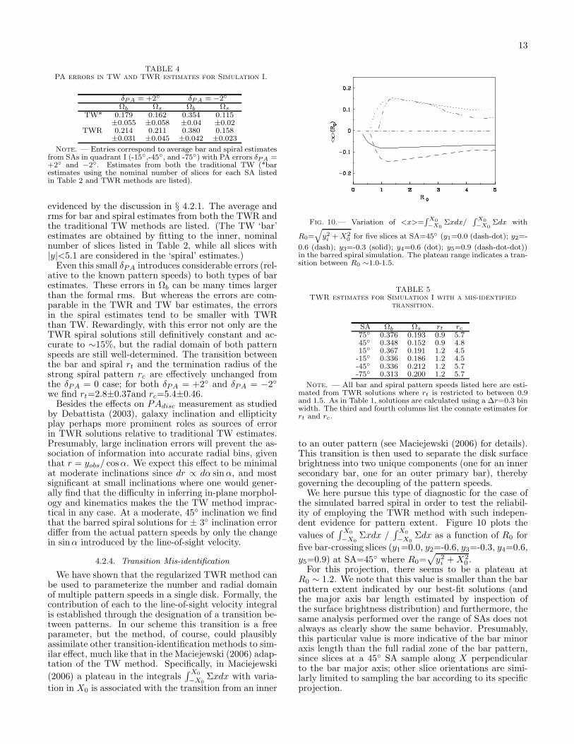
Fig. 10.— Variation of <x>=R X0

−X0Σxdx/

R X0

−X0Σdx with

R0=q

y2i +X2

0for five slices at SA=45 (y1=0.0 (dash-dot); y2=-

0.6 (dash); y3=-0.3 (solid); y4=0.6 (dot); y5=0.9 (dash-dot-dot))in the barred spiral simulation. The plateau range indicates a tran-sition between R0 ∼1.0-1.5.

TABLE 5TWR estimates for Simulation I with a mis-identified

transition.

SA Ωb Ωs rt rc75 0.376 0.193 0.9 5.745 0.348 0.152 0.9 4.815 0.367 0.191 1.2 4.5-15 0.336 0.186 1.2 4.5-45 0.336 0.212 1.2 5.7-75 0.313 0.200 1.2 5.7

Note. — All bar and spiral pattern speeds listed here are esti-mated from TWR solutions where rt is restricted to between 0.9and 1.5. As in Table 1, solutions are calculated using a ∆r=0.3 binwidth. The third and fourth columns list the connate estimates forrt and rc.

to an outer pattern (see Maciejewski (2006) for details).This transition is then used to separate the disk surfacebrightness into two unique components (one for an innersecondary bar, one for an outer primary bar), therebygoverning the decoupling of the pattern speeds.We here pursue this type of diagnostic for the case of

the simulated barred spiral in order to test the reliabil-ity of employing the TWR method with such indepen-dent evidence for pattern extent. Figure 10 plots the

values of∫X0

−X0Σxdx /

∫X0

−X0Σdx as a function of R0 for

five bar-crossing slices (y1=0.0, y2=-0.6, y3=-0.3, y4=0.6,

y5=0.9) at SA=45 where R0=√

y2i +X20 .

For this projection, there seems to be a plateau atR0 ∼ 1.2. We note that this value is smaller than the barpattern extent indicated by our best-fit solutions (andthe major axis bar length estimated by inspection ofthe surface brightness distribution) and furthermore, thesame analysis performed over the range of SAs does notalways as clearly show the same behavior. Presumably,this particular value is more indicative of the bar minoraxis length than the full radial zone of the bar pattern,since slices at a 45 SA sample along X perpendicularto the bar major axis; other slice orientations are simi-larly limited to sampling the bar according to its specificprojection.

14

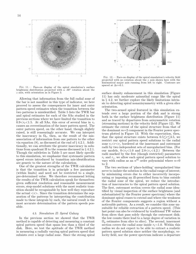
Fig. 11.— Face-on display of the spiral simulation’s surfacebrightness distribution projected with a -30 rotation about thez axis, with orientation as in Figure 3.

Allowing that information from the full radial zone ofthe bar is not manifest in this type of indicator, we hereproceed to assess the consequences for inner and outerpattern speed estimates when the transition between thetwo patterns is misidentified. Table 5 lists the TWR barand spiral estimates for each of the SAs studied in theprevious sections where we have limited the transition to0.9<rt<1.5. At all SAs, this error of several bins in rtcauses an overestimation of the inner pattern speed. Theouter pattern speed, on the other hand, though slightlyraised, is still reassuringly accurate. We can interpretthe inaccuracy in Ωb, then, as the result of the mis-association of information from one pattern to the othervia equation (8), as discussed at the end of § 4.2.1. Addi-tionally, we can attribute the greater inaccuracy in solu-tions from quadrant II to the reasons discussed in § 4.2.1.Though the subtleties in Table 5 are most likely specificto this simulation, we emphasize that systematic patternspeed errors introduced by transition mis-identificationare generic to the nature of the calculation.One of the greatest strengths of the TWR calculation

is that the transition is in principle a free parameter(within limits) and need not be restricted to a single,pre-determined value. We therefore recommend lettingthe results of the TWR calculation speak for themselves:given sufficient resolution and reasonable measurementerrors, step-model solutions with the most realistic tran-sition should be recognizable by how well they reproducethe actual <v>. Since the transition determines the sep-aration of the patterns by interpreting the contributionmade to these integrals by each, the natural result is themost accurate determination of the pattern speeds pos-sible.

4.3. Simulation II: Spiral Galaxy

In the previous section we showed that the TWRmethod is capable of detecting and measuring a constantspiral pattern speed that spans less than a third of thedisk. Here, we test the aptitude of the TWR methodin measuring a radially varying spiral pattern speed thatsubsists over a large radial zone. Since the strong spiral

Fig. 12.— Face-on display of the spiral simulation’s velocity fieldprojected with no rotation about the z axis shown here with thekinematical major axis running from left to right. Contours arespaced at ∆v=0.1.

surface density enhancement in this simulation (Figure11) has only moderate azimuthal range like the spiralin § 4.2, we further explore the likely limitations intrin-sic to detecting spiral nonaxisymmetry with a given sliceorientation.The two-armed spiral featured in this simulation ex-

tends over a large portion of the disk and is strongboth in the surface brightness distribution (Figure 11)and as traced by departures from axisymmetric rotation(streaming motions) in the velocity field (Figure 12). Weestimate the extent of the spiral structure from that ofthe dominantm=2 component in the Fourier power spec-trum plotted in Figure 13. With the expectation, then,that the spiral structure exists between 0.5.r.3.5, werestrict our spiral pattern speed solutions to the radialzone rt<r<rc bordered at the innermost and outermostradii by two independent sets of unregularized bins. (Forour models, 0<rt<1.0 and 2.8<rc<4.2.) Between theradii marked by the free (though restricted) parametersrt and rc, we allow each spiral pattern speed solution tovary with radius as an nth order polynomial where n=0to 2.The two sections of ‘place-holding’ unregularized bins

serve to isolate the solution in the radial range of interest;by minimizing errors due to either incorrectly incorpo-rating or imposing an ill-prescribed form to bins outsidethe radial zone of the spiral, we reduce the introduc-tion of inaccuracies to the spiral pattern speed solution.The first, outermost section covers the radial zone iden-tified by visual inspection of the surface brightness (andsubstantiated by the Fourier power spectrum) where thedominant spiral ceases to extend and where the weaknessof the Fourier components suggests a region without anoticeable pattern. As a result, we consider this zone un-suitable for reliable extraction of a pattern speed. (Thislast point can also be evidenced by traditional TW valuesfrom slices that pass solely through the outermost disk;the low counts there lead to a large degree of variation inΩp estimates from slice to slice). The second, innermostsection covers the radial zone inside rt∼1.0. Within thisradius we do not expect to be able to extract a realisticpattern speed solution since neither the morphology, ve-locity field, nor the power spectrum indicate a departure

15

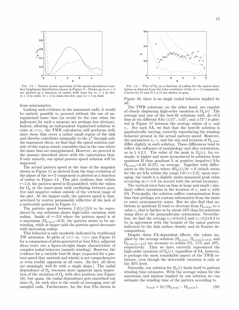
Fig. 13.— Fourier power spectrum of the spiral simulation’s sur-face brightness distribution shown in Figure 11. Modes up tom = 4are plotted as a function of radius with lines for m = 1 in dot,m = 2 in solid, m = 3 in dash-dot-dot, and m = 4 in dash.

from axisymmetry.Lacking such evidence in the innermost radii, it would

be entirely possible to proceed without the use of un-regularized inner bins (as would be the case when theindicators for such a measure are perhaps less obvious).Indeed, allowing an independent regularized solution toexist at r<rt, the TWR calculation still performs well;since these bins cover a rather small region of the diskand thereby contribute minimally to the χ2 through onlythe innermost slices, we find that the spiral solution out-side of this region closely resembles that in the case wherethe inner bins are unregularized. However, we proceed inthe manner described above with the expectation that,if only minorly, our spiral pattern speed solution will beimproved.The actual pattern speed at the time of the snapshot

shown in Figure 11 as derived from the time evolution ofthe phase of the m=2 component is plotted as a functionof radius in Figure 14. This plot confirms that withinr∼1.0, the pattern speed is ill-quantified, with the valuesfor Ωp at the inner-most radii oscillating between posi-tive and negative values outside of the vertical range ofthe plot. At the largest radii, the pattern speed is char-acterized by scatter presumably reflective of the lack ofa noticeable pattern in Figure 11.The pattern speed between 1.0.r.3.0 to be repro-

duced by our solutions shows high-order variation withradius. Inside of r∼2.0 where the pattern speed is ata maximum (Ωp,max∼0.3), the pattern seems to be un-winding, while at larger radii the pattern speed decreaseswith increasing radius.This behavior is only modestly indicated by traditional

TW estimates. In plots of <v> vs. <x> (see Figure 15for a comparison of plots generated at four SAs), adjacentslices trace out a figure-of-eight shape characteristic ofcomplex radial behavior (namely winding). However, theevidence for a variable best-fit slope (expected for a pat-tern speed that unwinds and winds) is not comprehensiveor even readily apparent in all cases. (In fact, all slicesare seemingly well fit with a single slope.) The radialdependence of Ωp becomes more apparent upon inspec-tion of the variation of Ωp with slice position (see Figure16), but again, the radial dependence gets smoothed outsince Ωp for each slice is the result of averaging over allsampled radii. Furthermore, for the four SAs shown in

Fig. 14.— Plot of Ωp as a function of radius for the spiral simu-lation as derived from the time evolution of the m = 2 component.Curves for Ω and Ω± κ/2 are shown in gray.

Figure 16, there is no single radial behavior implied byall.The TWR solutions, on the other hand, are capable

of clearly displaying high-order variation in Ωp(r). Theaverage and rms of the best-fit solutions with ∆r=0.2bins at six different SAs (±15, ±45, and ±75) is plot-ted in Figure 17 between the average values of rt andrc. For each SA, we find that the best-fit solution isquadratically varying, correctly reproducing the windingbehavior present in the actual pattern speed. However,the parameters rt, rc and the size and location of Ωp,max

differ slightly in each solution. These differences tend toreflect the influence of morphology and slice orientation,as in § 4.2.1. The value of the peak in Ωp(r), for ex-ample, is higher and more pronounced in solutions fromquadrant II than quadrant I; at positive (negative) SAsΩp,max∼0.34 (0.27), on average. Together with differ-ences in the location where dΩp(r)/dr = 0 (which variesfor the six SAs within the range 1.6<r<2.2), upon aver-aging, the result is a slightly under-measured peak valueoccurring at r∼1.8 (in accord with the actual location).The vertical error bars on bins at large and small r sim-

ilarly reflect variations in the location of rc and rt withSA. Principally, the solution suffers contamination frombins that perhaps yet contain information from the inneror outer axisymmetric zones. But we also find that so-lutions in quadrant II tend to decrease from Ωp,max to avalue rc that is further in by about 10% than for solutionsusing slices at the perpendicular orientation. Neverthe-less, we find the average rt=0.8±0.2 and rc=3.2±0.3 tobe in agreement with the bounds of the spiral patternindicated by the disk surface density and its Fourier de-composition.Despite these PA-dependent effects, the values im-

plied by the average solution (Ωp,max, Ωp,min|r=0.8, andΩp,min|r=3.2) are accurate to within 5%, 11% and 10%,respectively. That we have correctly reproduced thehigh-order variation of Ωp(r), regardless of SA, however,is perhaps the most remarkable aspect of the TWR so-lutions, even though the detectable variation is only atthe 30% level.Naturally, our solution for Ωp(r) lends itself to pattern

winding time estimates. With the average values for themaximum and minima implied by our solution we canestimate the winding time of the pattern according to

τwind = 2π/(Ωp,max − Ωp,min). (16)

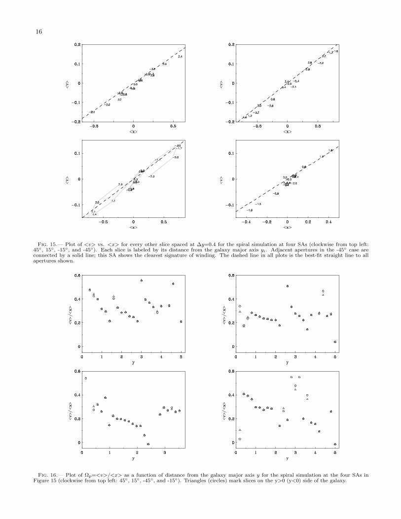
16

Fig. 15.— Plot of <v> vs. <x> for every other slice spaced at ∆y=0.4 for the spiral simulation at four SAs (clockwise from top left:45, 15, -15, and -45). Each slice is labeled by its distance from the galaxy major axis yi. Adjacent apertures in the -45 case areconnected by a solid line; this SA shows the clearest signature of winding. The dashed line in all plots is the best-fit straight line to allapertures shown.

Fig. 16.— Plot of Ωp=<v>/<x> as a function of distance from the galaxy major axis y for the spiral simulation at the four SAs inFigure 15 (clockwise from top left: 45, 15, -45, and -15). Triangles (circles) mark slices on the y>0 (y<0) side of the galaxy.

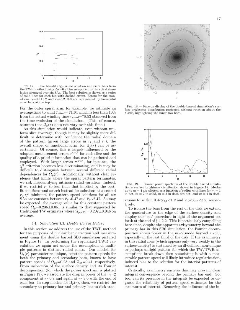
17

Fig. 17.— The best-fit regularized solution and error bars fromthe TWR method using ∆r=0.2 bins as applied to the spiral simu-lation averaged over six SAs. The best solution is shown as a seriesof solid lines for each bin with dashed errors. Errors for the tran-sitions rt=0.8±0.2 and rc=3.2±0.3 are represented by horizontalerror bars at the top.

For the outer spiral arm, for example, we estimate anaverage time to wind τwind= 71.64 which is less than 10%from the actual winding time τwind=78.53 observed fromthe time evolution of the simulation. (This, of course,assumes that Ωp(r) does not vary over this time.)As this simulation would indicate, even without uni-

form slice coverage, though it may be slightly more dif-ficult to determine with confidence the radial domainof the pattern (given large errors in rt and rc), theoverall shape, or functional form, for Ωp(r) can be as-certained. Of course, this is largely influenced by theadopted measurement errors σ<v> for each slice and thequality of a priori information that can be gathered andemployed. With larger errors σ<v>, for instance, theχ2 criterion becomes less discriminating, and it may bedifficult to distinguish between several different radialdependences for Ωp(r). Additionally, without clear ev-idence that limits where the spiral pattern terminates,we risk misidentifying intrinsic radial variation. Indeed,if we restrict rc to less than that implied by the best-fit solutions–and search instead for solutions at a secondrc-χ

2 minimum–the pattern speed solutions for all sixSAs are constant between rt∼0.47 and rc∼2.47. As maybe expected, the average value for this constant patternspeed Ωp=0.236±0.051 is similar to that suggested bytraditional TW estimates where Ωp,TW=0.207±0.046 onaverage.

4.4. Simulation III: Double Barred Galaxy

In this section we address the use of the TWR methodfor the purposes of nuclear bar detection and measure-ment using the double barred SB0 simulation picturedin Figure 18. In performing the regularized TWR cal-culation we again act under the assumption of multi-ple patterns in distinct radial zones. Our models forΩp(r) parameterize unique, constant pattern speeds forboth the primary and secondary bars, known to havepattern speeds of Ωpb=0.23 and Ωsb=0.41, respectively.From inspection of the surface density and its Fourierdecomposition (for which the power spectrum is plottedin Figure 19), we associate the drop in power of the m=2component at r∼0.8 and again at r∼3.0 with the end ofeach bar. In step-models for Ωp(r), then, we restrict thesecondary-to-primary bar and primary bar-to-disk tran-

Fig. 18.— Face-on display of the double barred simulation’s sur-face brightness distribution projected without rotation about thez axis, highlighting the inner two bars.

Fig. 19.— Fourier power spectrum of the double barred simula-tion’s surface brightness distribution shown in Figure 18. Modesup to m = 4 are plotted as a function of radius with lines for m = 1in dot, m = 2 in solid, m = 3 in dash-dot-dot, and m = 4 in dash.

sitions to within 0.4<rt,1<1.2 and 2.5<rt,2<3.2, respec-tively.To isolate the bars from the rest of the disk we extend

the quadrature to the edge of the surface density andemploy our ‘cut’ procedure in light of the argument setforth at the end of § 4.2.2. This is particularly compellinghere since, despite the apparent axisymmetry beyond theprimary bar in this SB0 simulation, the Fourier decom-position shows power in the m=2 mode beyond r∼3.0,especially in the last third of the disk. If the asymmetryin this radial zone (which appears only very weakly in thesurface density) is sustained by an ill-defined, non-uniqueor perhaps unrigid pattern–for which the TW/TWR as-sumptions break-down–then associating it with a mea-surable pattern speed will likely introduce regularization-induced bias to the solution for the interior patterns ofinterest.Critically, asymmetry such as this may prevent clear

integral convergence beyond the primary bar end. So,too, can its presence in the integrals be expected to de-grade the reliability of pattern speed estimates for thestructures of interest. Removing the influence of the in-

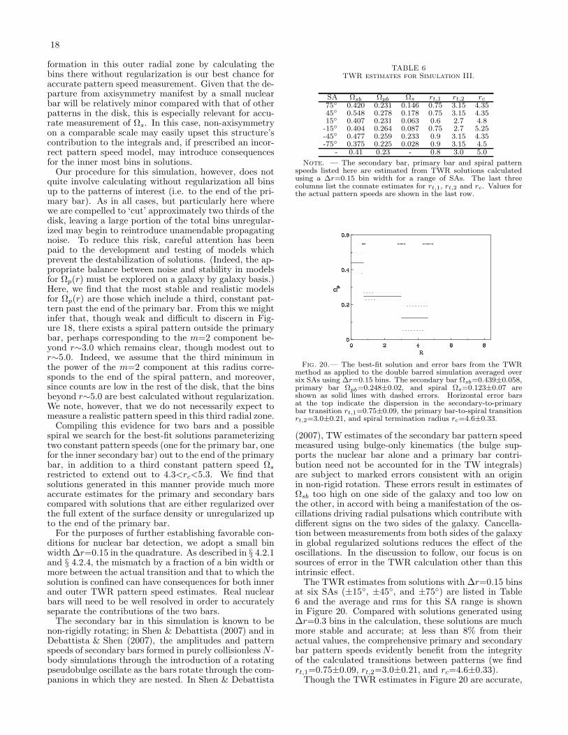
18

formation in this outer radial zone by calculating thebins there without regularization is our best chance foraccurate pattern speed measurement. Given that the de-parture from axisymmetry manifest by a small nuclearbar will be relatively minor compared with that of otherpatterns in the disk, this is especially relevant for accu-rate measurement of Ωs. In this case, non-axisymmetryon a comparable scale may easily upset this structure’scontribution to the integrals and, if prescribed an incor-rect pattern speed model, may introduce consequencesfor the inner most bins in solutions.Our procedure for this simulation, however, does not

quite involve calculating without regularization all binsup to the patterns of interest (i.e. to the end of the pri-mary bar). As in all cases, but particularly here wherewe are compelled to ‘cut’ approximately two thirds of thedisk, leaving a large portion of the total bins unregular-ized may begin to reintroduce unamendable propagatingnoise. To reduce this risk, careful attention has beenpaid to the development and testing of models whichprevent the destabilization of solutions. (Indeed, the ap-propriate balance between noise and stability in modelsfor Ωp(r) must be explored on a galaxy by galaxy basis.)Here, we find that the most stable and realistic modelsfor Ωp(r) are those which include a third, constant pat-tern past the end of the primary bar. From this we mightinfer that, though weak and difficult to discern in Fig-ure 18, there exists a spiral pattern outside the primarybar, perhaps corresponding to the m=2 component be-yond r∼3.0 which remains clear, though modest out tor∼5.0. Indeed, we assume that the third minimum inthe power of the m=2 component at this radius corre-sponds to the end of the spiral pattern, and moreover,since counts are low in the rest of the disk, that the binsbeyond r∼5.0 are best calculated without regularization.We note, however, that we do not necessarily expect tomeasure a realistic pattern speed in this third radial zone.Compiling this evidence for two bars and a possible

spiral we search for the best-fit solutions parameterizingtwo constant pattern speeds (one for the primary bar, onefor the inner secondary bar) out to the end of the primarybar, in addition to a third constant pattern speed Ωs

restricted to extend out to 4.3<rc<5.3. We find thatsolutions generated in this manner provide much moreaccurate estimates for the primary and secondary barscompared with solutions that are either regularized overthe full extent of the surface density or unregularized upto the end of the primary bar.For the purposes of further establishing favorable con-

ditions for nuclear bar detection, we adopt a small binwidth ∆r=0.15 in the quadrature. As described in § 4.2.1and § 4.2.4, the mismatch by a fraction of a bin width ormore between the actual transition and that to which thesolution is confined can have consequences for both innerand outer TWR pattern speed estimates. Real nuclearbars will need to be well resolved in order to accuratelyseparate the contributions of the two bars.The secondary bar in this simulation is known to be

non-rigidly rotating; in Shen & Debattista (2007) and inDebattista & Shen (2007), the amplitudes and patternspeeds of secondary bars formed in purely collisionlessN -body simulations through the introduction of a rotatingpseudobulge oscillate as the bars rotate through the com-panions in which they are nested. In Shen & Debattista

TABLE 6TWR estimates for Simulation III.

SA Ωsb Ωpb Ωs rt,1 rt,2 rc75 0.420 0.231 0.146 0.75 3.15 4.3545 0.548 0.278 0.178 0.75 3.15 4.3515 0.407 0.231 0.063 0.6 2.7 4.8-15 0.404 0.264 0.087 0.75 2.7 5.25-45 0.477 0.259 0.233 0.9 3.15 4.35-75 0.375 0.225 0.028 0.9 3.15 4.5

- 0.41 0.23 - 0.8 3.0 5.0

Note. — The secondary bar, primary bar and spiral patternspeeds listed here are estimated from TWR solutions calculatedusing a ∆r=0.15 bin width for a range of SAs. The last threecolumns list the connate estimates for rt,1, rt,2 and rc. Values forthe actual pattern speeds are shown in the last row.

Fig. 20.— The best-fit solution and error bars from the TWRmethod as applied to the double barred simulation averaged oversix SAs using ∆r=0.15 bins. The secondary bar Ωsb=0.439±0.058,primary bar Ωpb=0.248±0.02, and spiral Ωs=0.123±0.07 areshown as solid lines with dashed errors. Horizontal error barsat the top indicate the dispersion in the secondary-to-primarybar transition rt,1=0.75±0.09, the primary bar-to-spiral transitionrt,2=3.0±0.21, and spiral termination radius rc=4.6±0.33.

(2007), TW estimates of the secondary bar pattern speedmeasured using bulge-only kinematics (the bulge sup-ports the nuclear bar alone and a primary bar contri-bution need not be accounted for in the TW integrals)are subject to marked errors consistent with an originin non-rigid rotation. These errors result in estimates ofΩsb too high on one side of the galaxy and too low onthe other, in accord with being a manifestation of the os-cillations driving radial pulsations which contribute withdifferent signs on the two sides of the galaxy. Cancella-tion between measurements from both sides of the galaxyin global regularized solutions reduces the effect of theoscillations. In the discussion to follow, our focus is onsources of error in the TWR calculation other than thisintrinsic effect.The TWR estimates from solutions with ∆r=0.15 bins

at six SAs (±15, ±45, and ±75) are listed in Table6 and the average and rms for this SA range is shownin Figure 20. Compared with solutions generated using∆r=0.3 bins in the calculation, these solutions are muchmore stable and accurate; at less than 8% from theiractual values, the comprehensive primary and secondarybar pattern speeds evidently benefit from the integrityof the calculated transitions between patterns (we findrt,1=0.75±0.09, rt,2=3.0±0.21, and rc=4.6±0.33).Though the TWR estimates in Figure 20 are accurate,

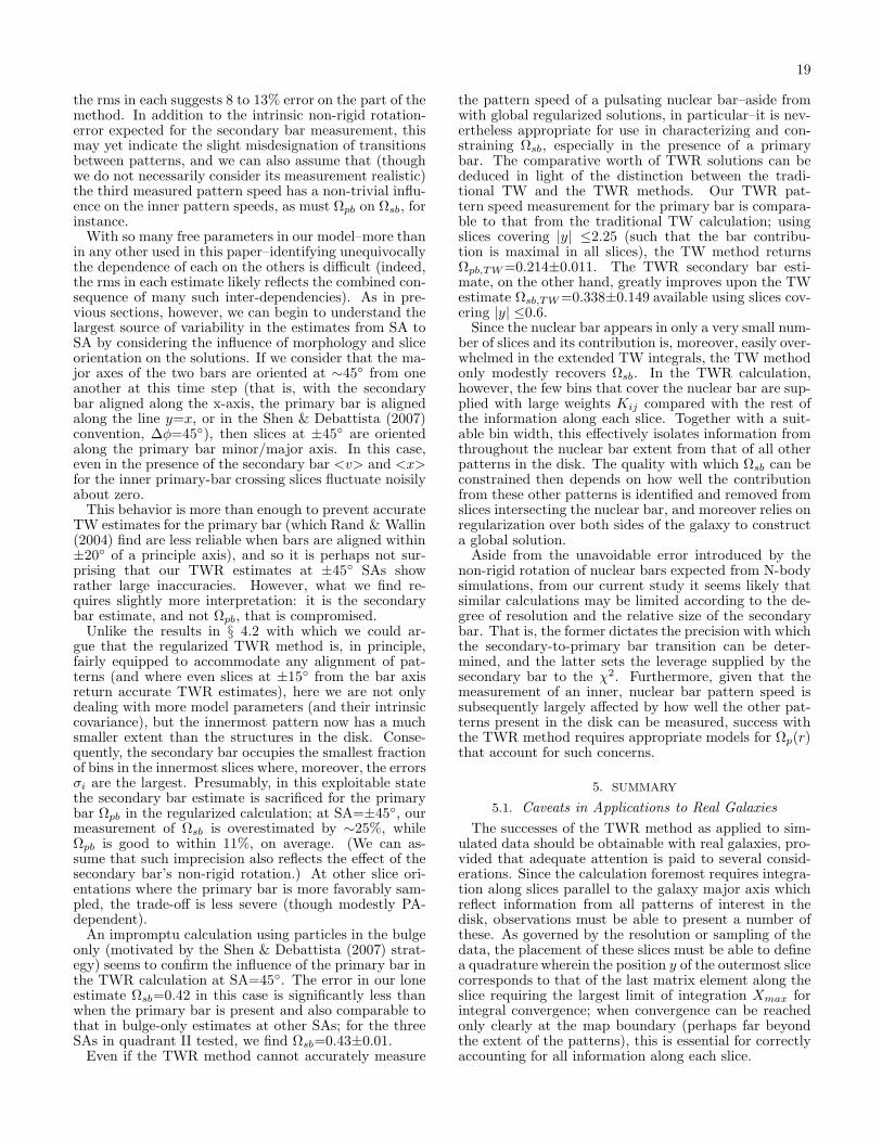
19

the rms in each suggests 8 to 13% error on the part of themethod. In addition to the intrinsic non-rigid rotation-error expected for the secondary bar measurement, thismay yet indicate the slight misdesignation of transitionsbetween patterns, and we can also assume that (thoughwe do not necessarily consider its measurement realistic)the third measured pattern speed has a non-trivial influ-ence on the inner pattern speeds, as must Ωpb on Ωsb, forinstance.With so many free parameters in our model–more than

in any other used in this paper–identifying unequivocallythe dependence of each on the others is difficult (indeed,the rms in each estimate likely reflects the combined con-sequence of many such inter-dependencies). As in pre-vious sections, however, we can begin to understand thelargest source of variability in the estimates from SA toSA by considering the influence of morphology and sliceorientation on the solutions. If we consider that the ma-jor axes of the two bars are oriented at ∼45 from oneanother at this time step (that is, with the secondarybar aligned along the x-axis, the primary bar is alignedalong the line y=x, or in the Shen & Debattista (2007)convention, ∆φ=45), then slices at ±45 are orientedalong the primary bar minor/major axis. In this case,even in the presence of the secondary bar <v> and <x>for the inner primary-bar crossing slices fluctuate noisilyabout zero.This behavior is more than enough to prevent accurate

TW estimates for the primary bar (which Rand & Wallin(2004) find are less reliable when bars are aligned within±20 of a principle axis), and so it is perhaps not sur-prising that our TWR estimates at ±45 SAs showrather large inaccuracies. However, what we find re-quires slightly more interpretation: it is the secondarybar estimate, and not Ωpb, that is compromised.Unlike the results in § 4.2 with which we could ar-

gue that the regularized TWR method is, in principle,fairly equipped to accommodate any alignment of pat-terns (and where even slices at ±15 from the bar axisreturn accurate TWR estimates), here we are not onlydealing with more model parameters (and their intrinsiccovariance), but the innermost pattern now has a muchsmaller extent than the structures in the disk. Conse-quently, the secondary bar occupies the smallest fractionof bins in the innermost slices where, moreover, the errorsσi are the largest. Presumably, in this exploitable statethe secondary bar estimate is sacrificed for the primarybar Ωpb in the regularized calculation; at SA=±45, ourmeasurement of Ωsb is overestimated by ∼25%, whileΩpb is good to within 11%, on average. (We can as-sume that such imprecision also reflects the effect of thesecondary bar’s non-rigid rotation.) At other slice ori-entations where the primary bar is more favorably sam-pled, the trade-off is less severe (though modestly PA-dependent).An impromptu calculation using particles in the bulge

only (motivated by the Shen & Debattista (2007) strat-egy) seems to confirm the influence of the primary bar inthe TWR calculation at SA=45. The error in our loneestimate Ωsb=0.42 in this case is significantly less thanwhen the primary bar is present and also comparable tothat in bulge-only estimates at other SAs; for the threeSAs in quadrant II tested, we find Ωsb=0.43±0.01.Even if the TWR method cannot accurately measure

the pattern speed of a pulsating nuclear bar–aside fromwith global regularized solutions, in particular–it is nev-ertheless appropriate for use in characterizing and con-straining Ωsb, especially in the presence of a primarybar. The comparative worth of TWR solutions can bededuced in light of the distinction between the tradi-tional TW and the TWR methods. Our TWR pat-tern speed measurement for the primary bar is compara-ble to that from the traditional TW calculation; usingslices covering |y| ≤2.25 (such that the bar contribu-tion is maximal in all slices), the TW method returnsΩpb,TW=0.214±0.011. The TWR secondary bar esti-mate, on the other hand, greatly improves upon the TWestimate Ωsb,TW=0.338±0.149 available using slices cov-ering |y| ≤0.6.Since the nuclear bar appears in only a very small num-

ber of slices and its contribution is, moreover, easily over-whelmed in the extended TW integrals, the TW methodonly modestly recovers Ωsb. In the TWR calculation,however, the few bins that cover the nuclear bar are sup-plied with large weights Kij compared with the rest ofthe information along each slice. Together with a suit-able bin width, this effectively isolates information fromthroughout the nuclear bar extent from that of all otherpatterns in the disk. The quality with which Ωsb can beconstrained then depends on how well the contributionfrom these other patterns is identified and removed fromslices intersecting the nuclear bar, and moreover relies onregularization over both sides of the galaxy to constructa global solution.Aside from the unavoidable error introduced by the

non-rigid rotation of nuclear bars expected from N-bodysimulations, from our current study it seems likely thatsimilar calculations may be limited according to the de-gree of resolution and the relative size of the secondarybar. That is, the former dictates the precision with whichthe secondary-to-primary bar transition can be deter-mined, and the latter sets the leverage supplied by thesecondary bar to the χ2. Furthermore, given that themeasurement of an inner, nuclear bar pattern speed issubsequently largely affected by how well the other pat-terns present in the disk can be measured, success withthe TWR method requires appropriate models for Ωp(r)that account for such concerns.

5. SUMMARY

5.1. Caveats in Applications to Real Galaxies

The successes of the TWR method as applied to sim-ulated data should be obtainable with real galaxies, pro-vided that adequate attention is paid to several consid-erations. Since the calculation foremost requires integra-tion along slices parallel to the galaxy major axis whichreflect information from all patterns of interest in thedisk, observations must be able to present a number ofthese. As governed by the resolution or sampling of thedata, the placement of these slices must be able to definea quadrature wherein the position y of the outermost slicecorresponds to that of the last matrix element along theslice requiring the largest limit of integration Xmax forintegral convergence; when convergence can be reachedonly clearly at the map boundary (perhaps far beyondthe extent of the patterns), this is essential for correctlyaccounting for all information along each slice.

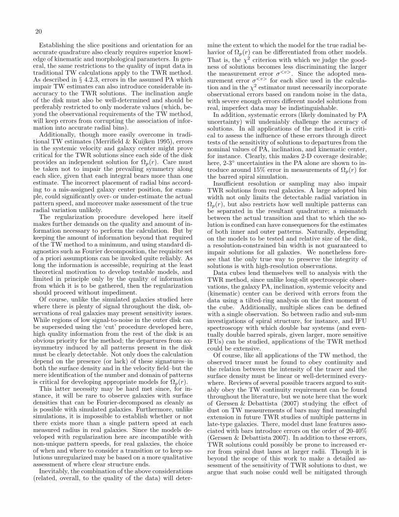
20

Establishing the slice positions and orientation for anaccurate quadrature also clearly requires superior knowl-edge of kinematic and morphological parameters. In gen-eral, the same restrictions to the quality of input data intraditional TW calculations apply to the TWR method.As described in § 4.2.3, errors in the assumed PA whichimpair TW estimates can also introduce considerable in-accuracy to the TWR solutions. The inclination angleof the disk must also be well-determined and should bepreferably restricted to only moderate values (which, be-yond the observational requirements of the TW method,will keep errors from corrupting the association of infor-mation into accurate radial bins).Additionally, though more easily overcome in tradi-

tional TW estimates (Merrifield & Kuijken 1995), errorsin the systemic velocity and galaxy center might provecritical for the TWR solutions since each side of the diskprovides an independent solution for Ωp(r). Care mustbe taken not to impair the prevailing symmetry alongeach slice, given that each integral bears more than oneestimate. The incorrect placement of radial bins accord-ing to a mis-assigned galaxy center position, for exam-ple, could significantly over- or under-estimate the actualpattern speed, and moreover make assessment of the trueradial variation unlikely.The regularization procedure developed here itself

makes further demands on the quality and amount of in-formation necessary to perform the calculation. But bykeeping the amount of information beyond that requiredof the TW method to a minimum, and using standard di-agnostics such as Fourier decomposition, the requisite setof a priori assumptions can be invoked quite reliably. Aslong the information is accessible, requiring at the leasttheoretical motivation to develop testable models, andlimited in principle only by the quality of informationfrom which it is to be gathered, then the regularizationshould proceed without impediment.Of course, unlike the simulated galaxies studied here

where there is plenty of signal throughout the disk, ob-servations of real galaxies may present sensitivity issues.While regions of low signal-to-noise in the outer disk canbe superseded using the ‘cut’ procedure developed here,high quality information from the rest of the disk is anobvious priority for the method; the departures from ax-isymmetry induced by all patterns present in the diskmust be clearly detectable. Not only does the calculationdepend on the presence (or lack) of these signatures–inboth the surface density and in the velocity field–but themere identification of the number and domain of patternsis critical for developing appropriate models for Ωp(r).This latter necessity may be hard met since, for in-

stance, it will be rare to observe galaxies with surfacedensities that can be Fourier-decomposed as cleanly asis possible with simulated galaxies. Furthermore, unlikesimulations, it is impossible to establish whether or notthere exists more than a single pattern speed at eachmeasured radius in real galaxies. Since the models de-veloped with regularization here are incompatible withnon-unique pattern speeds, for real galaxies, the choiceof when and where to consider a transition or to keep so-lutions unregularized may be based on a more qualitativeassessment of where clear structure ends.Inevitably, the combination of the above considerations

(related, overall, to the quality of the data) will deter-

mine the extent to which the model for the true radial be-havior of Ωp(r) can be differentiated from other models.That is, the χ2 criterion with which we judge the good-ness of solutions becomes less discriminating the largerthe measurement error σ<v>. Since the adopted mea-surement error σ<v> for each slice used in the calcula-tion and in the χ2 estimator must necessarily incorporateobservational errors based on random noise in the data,with severe enough errors different model solutions fromreal, imperfect data may be indistinguishable.In addition, systematic errors (likely dominated by PA

uncertainty) will undeniably challenge the accuracy ofsolutions. In all applications of the method it is criti-cal to assess the influence of these errors through directtests of the sensitivity of solutions to departures from thenominal values of PA, inclination, and kinematic center,for instance. Clearly, this makes 2-D coverage desirable;here, 2-3 uncertainties in the PA alone are shown to in-troduce around 15% error in measurements of Ωp(r) forthe barred spiral simulation.Insufficient resolution or sampling may also impair

TWR solutions from real galaxies. A large adopted binwidth not only limits the detectable radial variation inΩp(r), but also restricts how well multiple patterns canbe separated in the resultant quadrature; a mismatchbetween the actual transition and that to which the so-lution is confined can have consequences for the estimatesof both inner and outer patterns. Naturally, dependingon the models to be tested and relative size of the disk,a resolution-constrained bin width is not guaranteed toimpair solutions for all galaxies. We nonetheless fore-see that the only true way to preserve the integrity ofsolutions is with high-resolution observations.Data cubes lend themselves well to analysis with the

TWR method, since unlike long-slit spectroscopic obser-vations, the galaxy PA, inclination, systemic velocity and(kinematic) center can be derived with errors from thedata using a tilted-ring analysis on the first moment ofthe cube. Additionally, multiple slices can be definedwith a single observation. So between radio and sub-mminvestigations of spiral structure, for instance, and IFUspectroscopy with which double bar systems (and even-tually double barred spirals, given larger, more sensitiveIFUs) can be studied, applications of the TWR methodcould be extensive.Of course, like all applications of the TW method, the

observed tracer must be found to obey continuity andthe relation between the intensity of the tracer and thesurface density must be linear or well-determined every-where. Reviews of several possible tracers argued to suit-ably obey the TW continuity requirement can be foundthroughout the literature, but we note here that the workof Gerssen & Debattista (2007) studying the effect ofdust on TW measurements of bars may find meaningfulextension in future TWR studies of multiple patterns inlate-type galaxies. There, model dust lane features asso-ciated with bars introduce errors on the order of 20-40%(Gerssen & Debattista 2007). In addition to these errors,TWR solutions could possibly be prone to increased er-ror from spiral dust lanes at larger radii. Though it isbeyond the scope of this work to make a detailed as-sessment of the sensitivity of TWR solutions to dust, weargue that such noise could well be mitigated through

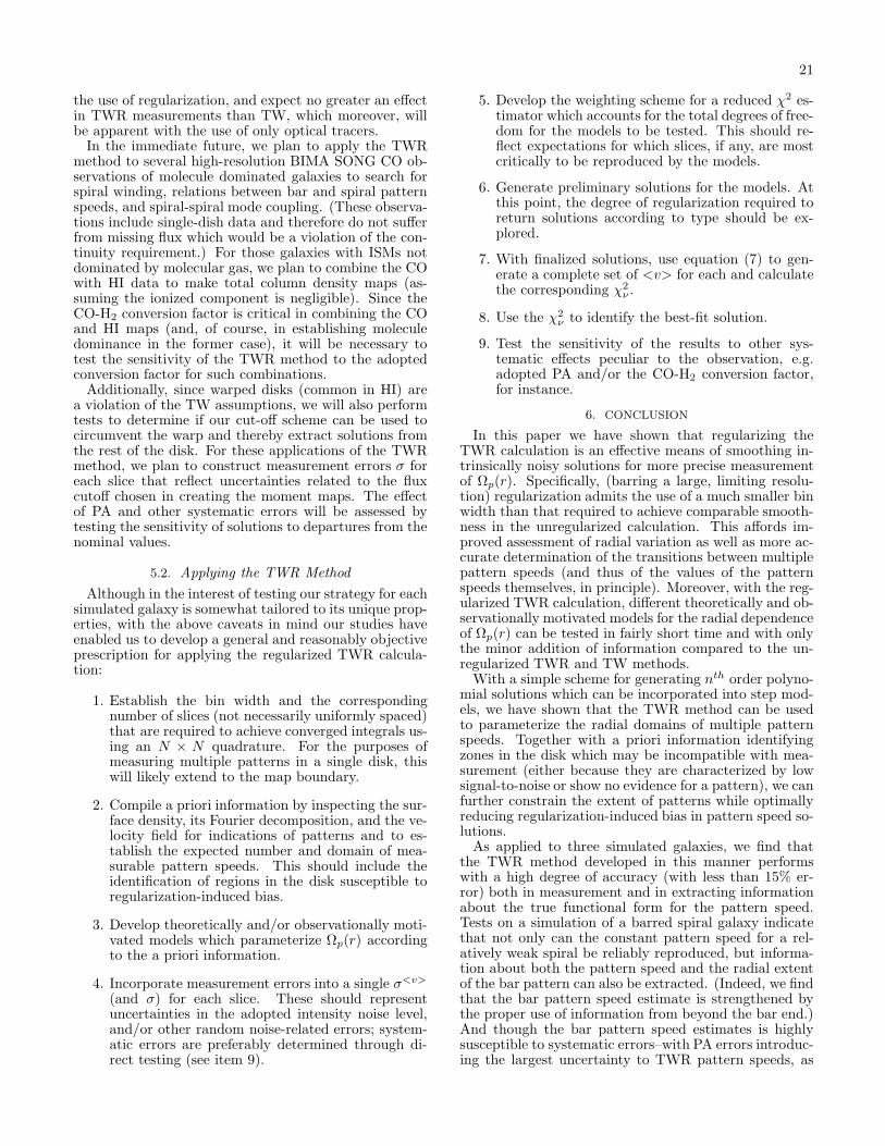
21

the use of regularization, and expect no greater an effectin TWR measurements than TW, which moreover, willbe apparent with the use of only optical tracers.In the immediate future, we plan to apply the TWR

method to several high-resolution BIMA SONG CO ob-servations of molecule dominated galaxies to search forspiral winding, relations between bar and spiral patternspeeds, and spiral-spiral mode coupling. (These observa-tions include single-dish data and therefore do not sufferfrom missing flux which would be a violation of the con-tinuity requirement.) For those galaxies with ISMs notdominated by molecular gas, we plan to combine the COwith HI data to make total column density maps (as-suming the ionized component is negligible). Since theCO-H2 conversion factor is critical in combining the COand HI maps (and, of course, in establishing moleculedominance in the former case), it will be necessary totest the sensitivity of the TWR method to the adoptedconversion factor for such combinations.Additionally, since warped disks (common in HI) are

a violation of the TW assumptions, we will also performtests to determine if our cut-off scheme can be used tocircumvent the warp and thereby extract solutions fromthe rest of the disk. For these applications of the TWRmethod, we plan to construct measurement errors σ foreach slice that reflect uncertainties related to the fluxcutoff chosen in creating the moment maps. The effectof PA and other systematic errors will be assessed bytesting the sensitivity of solutions to departures from thenominal values.

5.2. Applying the TWR Method

Although in the interest of testing our strategy for eachsimulated galaxy is somewhat tailored to its unique prop-erties, with the above caveats in mind our studies haveenabled us to develop a general and reasonably objectiveprescription for applying the regularized TWR calcula-tion:

1. Establish the bin width and the correspondingnumber of slices (not necessarily uniformly spaced)that are required to achieve converged integrals us-ing an N × N quadrature. For the purposes ofmeasuring multiple patterns in a single disk, thiswill likely extend to the map boundary.

2. Compile a priori information by inspecting the sur-face density, its Fourier decomposition, and the ve-locity field for indications of patterns and to es-tablish the expected number and domain of mea-surable pattern speeds. This should include theidentification of regions in the disk susceptible toregularization-induced bias.

3. Develop theoretically and/or observationally moti-vated models which parameterize Ωp(r) accordingto the a priori information.

4. Incorporate measurement errors into a single σ<v>

(and σ) for each slice. These should representuncertainties in the adopted intensity noise level,and/or other random noise-related errors; system-atic errors are preferably determined through di-rect testing (see item 9).

5. Develop the weighting scheme for a reduced χ2 es-timator which accounts for the total degrees of free-dom for the models to be tested. This should re-flect expectations for which slices, if any, are mostcritically to be reproduced by the models.

6. Generate preliminary solutions for the models. Atthis point, the degree of regularization required toreturn solutions according to type should be ex-plored.

7. With finalized solutions, use equation (7) to gen-erate a complete set of <v> for each and calculatethe corresponding χ2

ν .

8. Use the χ2ν to identify the best-fit solution.

9. Test the sensitivity of the results to other sys-tematic effects peculiar to the observation, e.g.adopted PA and/or the CO-H2 conversion factor,for instance.

6. CONCLUSION

In this paper we have shown that regularizing theTWR calculation is an effective means of smoothing in-trinsically noisy solutions for more precise measurementof Ωp(r). Specifically, (barring a large, limiting resolu-tion) regularization admits the use of a much smaller binwidth than that required to achieve comparable smooth-ness in the unregularized calculation. This affords im-proved assessment of radial variation as well as more ac-curate determination of the transitions between multiplepattern speeds (and thus of the values of the patternspeeds themselves, in principle). Moreover, with the reg-ularized TWR calculation, different theoretically and ob-servationally motivated models for the radial dependenceof Ωp(r) can be tested in fairly short time and with onlythe minor addition of information compared to the un-regularized TWR and TW methods.With a simple scheme for generating nth order polyno-

mial solutions which can be incorporated into step mod-els, we have shown that the TWR method can be usedto parameterize the radial domains of multiple patternspeeds. Together with a priori information identifyingzones in the disk which may be incompatible with mea-surement (either because they are characterized by lowsignal-to-noise or show no evidence for a pattern), we canfurther constrain the extent of patterns while optimallyreducing regularization-induced bias in pattern speed so-lutions.As applied to three simulated galaxies, we find that

the TWR method developed in this manner performswith a high degree of accuracy (with less than 15% er-ror) both in measurement and in extracting informationabout the true functional form for the pattern speed.Tests on a simulation of a barred spiral galaxy indicatethat not only can the constant pattern speed for a rel-atively weak spiral be reliably reproduced, but informa-tion about both the pattern speed and the radial extentof the bar pattern can also be extracted. (Indeed, we findthat the bar pattern speed estimate is strengthened bythe proper use of information from beyond the bar end.)And though the bar pattern speed estimates is highlysusceptible to systematic errors–with PA errors introduc-ing the largest uncertainty to TWR pattern speeds, as

22

with TW estimates–we find that the identification of thetransition between the two is relatively stable.The TWR method can also be effectively employed

to measure patterns that are winding in nature. In asimulation of a two-armed spiral, the best-fit TWR solu-tions from several slice orientations correctly reproducethe high-order radial variation of the pattern speed, de-spite modest indication that not all orientations supplythe same authority (this, of course, would seem to dependon the morphology of this spiral, in particular). Indeed,though the TWR method can, in principle, handle any(presumably random) alignment of patterns, in all of thesimulations studied, slice orientations which provide themost uniform coverage of the patterns are preferred. Thisis of particular importance for nuclear bar pattern speedmeasurement, as found in tests of the method on a dou-ble barred simulation. Since the innermost bins whichprovide the foremost leverage on the nuclear bar are alsothe most susceptible to errors from throughout the disk,confident measurement requires all other patterns to bewell constrained.In principle, comparable accuracy should be achievable

on real galaxies. However, these tests do not constrainhow well the TWR method can perform under severe ob-servational limitations which may commonly arise. Notonly can determinations of the PA, inclination, and dy-namical center be subject to considerable errors givenlow-quality data, but identifying constraints on the pat-terns present in the disk to be incorporated into modelsfor Ωp(r) could prove challenging. Additionally, thoughregularization can reduce the impact of noise on solu-

tions, large measurement errors for each slice could makediscriminating between several possible models for Ωp(r)difficult. And most critically, since the nature of the nu-merical calculation relies on a relatively small bin widthto achieve its greatest accuracy, without high resolution,some observations may not afford practical solutions.Nevertheless, if restricted to high resolution obser-

vations with adequate sensitivity, and given radiallystable kinematic parameters, TWR solutions can beused to study the connection between multiple patternsand the nature of spiral winding. So, too, can weexpect progressively more satisfactory applications ofthe method; though the number of galaxies to whichthe method can be successfully applied is limited bythe current generation of instruments, in the future,larger IFUs, ALMA, and eventually, SKA should yieldmuch higher quality data with larger areal coverage andhigher angular resolution. This prospect in itself shouldwarrant future studies with the TWR method.

This research was supported in part by NASA throughthe American Astronomical Society’s Small ResearchGrant Program. S. E. M. acknowledges support froma NASA-funded New Mexico Space Grant ConsortiumGraduate Research Fellowship. V. P. D. is supported byan RCUK Fellowship at the University of Central Lan-cashire. J. S. acknowledges support from a Harlan J.Smith fellowship. This material is based on work par-tially supported by the National Science Foundation un-der grant AST 03-06958 to R. J. R.

REFERENCES

Corsini, E. M., Debattista, V. P., Aguerri, J. A. L. 2003, ApJ,599, L29

Debattista, V. P. & Sellwood, J. A. 1998, ApJ, 493, L5Debattista, V. P. & Sellwood, J. A. 2000, ApJ, 543, 704Debattista, V. P. & Shen, J. 2007, ApJ, 654, 127Debattista, V. P., Corsini, E. M. & Aguerri, J. A. L. 2002,

MNRAS, 332, 65Debattista, V. P., Gerhard, O., Sevenster, M. N. 2002, MNRAS,

334, 355Debattista, V. P. 2003, MNRAS, 342, 1194Debattista, V. P. & Williams, T. B. 2004, ApJ, 605, 714Debattista, V. P., Mayer, L., Carollo, C. M., Moore, B., Wadsley,

J. & Quinn, T. 2006, ApJ, 645, 209Elmegreen, B. G., Elmegreen, D. M., Seiden, P. E. 1989, ApJ,

343, 602Elmegreen, B. G., Elmegreen, D. M., Chromey, F. R.,

Hasselbacher, D. A. & Bissell, B. A. 1996, AJ, 111, 2233Fathi, K., Toonen, S., Falcon-Barroso, J., Beckman, J. E.,

Hernandez, O., Daigle, O., Carignan, C. & de Zeeuw, T. 2007,ApJL, 667, 137

Garcia-Burillo, S., Combes, F., Gerin, M. 1993, A&A, 274, 148Gerssen, J. & Debattista, V. P. 2007, MNRAS, 378, 189Kormendy, J. & Norman, C. A. 1979, ApJ, 233, 539

Maciejewski, W. 2006, MNRAS, 371, 451Masset, F. & Tagger, M. 1997, A&A, 318, 747Merrifield, M. R. & Kuijken, K. 1995, MNRAS, 274, 933Merrifield, M. R., Rand, R. J., & Meidt, S. E. 2006, MNRAS,

366, 17Miller, K. 1970, SIAM Journal on Mathematical Analysis, Vol 1,

52Rand, R. J. & Wallin, J. F. 2004, ApJ, 614, 142Rautiainen, P. & Salo, H. 1999, A&A, 348, 737Rautiainen, P. & Salo, H. 2005, ApJL, 631, 129Roberts, W. & Stewart, G. 1987, ApJ, 314, 10Sellwood, J. A. & Kahn, F. D. 1991, MNRAS, 250, 278Sellwood, J. A. & Lin, D. N. C. 1989, MNRAS, 240, 991Sellwood, J. A. & Sparke, L. S. 1988, MNRAS, 231, 25

Shen, J. & Debattista, V. P. 2007, in preparationSygnet, J. F., Tagger, M., Athanassoula, E. & Pellat, R. 1988,

MNRAS, 232, 733Tikhonov, A. N. & Arsenin, V. Y. 1997, Solutions of Ill-posed

Problems (New York: Wiley)Tremaine, S. & Weinberg, M. D. 1984, ApJ 282, L5Zimmer, P., Rand, R. J. & McGraw, J. T. 2004, ApJ, 607, 285