Asymptotical Computations for

a Model of Flow in Saturated Porous Media

P. Amodio a, C.J. Budd b, O. Koch c,∗, G. Settanni d,E. Weinmuller c

aDipartimento di Matematica, Universita di Barivia E. Orabona 4, 70125 Bari, Italy

bMathematical Sciences, University of BathBath BA2 7AY, United Kingdom

cInstitute for Analysis and Scientific Computing (E101),Vienna University of Technology,

Wiedner Hauptstrasse 8–10, A-1040 Wien, AustriadDipartimento di Matematica e Fisica ‘E. De Giorgi’, Universita del Salento,

via per Arnesano, 73047 Monteroni di Lecce, Lecce, Italy

Abstract

We discuss an initial value problem for an implicit second order ordinary differentialequation which arises in models of flow in saturated porous media such as concrete.Depending on the initial condition, the solution features a sharp interface withderivatives which become numerically unbounded. By using an integrator based onfinite difference methods and equipped with adaptive step size selection, it is possibleto compute the solution on highly irregular meshes. In this way it is possible to verifyand predict asymptotical theory near the interface with remarkable accuracy.

Key words: Flow in concrete; Interface problem; Adaptive mesh selection;Asymptotic theory.1991 MSC: 65L05; 65L12; 34E99.

∗ Corresponding author.Email addresses: pierluigi.amodio@uniba.it (P. Amodio),

mascjb@bath.ac.uk (C.J. Budd), othmar@othmar-koch.org (O. Koch),giuseppina.settanni@unisalento.it (G. Settanni),e.weinmueller@tuwien.ac.at (E. Weinmuller).

Preprint submitted to Elsevier 19 December 2013

1 Introduction and Problem Statement

A model for the time dependent flow of water through a variably saturatedporous medium with exponential diffusivity, such as soil, rock or concrete isgiven by

∂u

∂t=

∂

∂x

(

D(u)∂u

∂x

)

, x ∈ [0,∞), t > 0, (1)

u(0, t) = ui, u(∞, t) = uo, uo < ui, u(x, 0) = u0(x), (2)

where u(x, t) is the saturation and is the fraction by volume of the pore spaceoccupied by the liquid a distance x into the porous medium, and

D(u) = D0eβu, β large.

In this problem the bulk of the liquid resides in the interval x ∈ [0, x∗(t)] wherethe moving interface x∗(t) is called the wetting front, and u≪ 1 if x > x∗. Thesolution changes very rapidly close to the wetting front, making (1)–(2) a chal-lenging problem both in analysis and in computation. The physical derivationof this equation is given in [8,12,15]. The numerical treatment of this prob-lem was first discussed in [20]. A detailed discussion of numerical methods forflow in porous media is given for instance in [11]. Similarity solutions of theproblem have been studied extensively in earlier work and [13] gives a compre-hensive overview of analytical results for various types of nonlinear diffusionequations. In [13], the similarity solution for exponential diffusivity (3)–(5)below is derived. In [18], an iterative approach to solving this problem is de-veloped. The paper [6] gives an asymptotic series expansion for the similaritysolution under certain simplifying assumptions. Further asymptotic analysis ofthe similarity solution is developed in [16,17]. However, there has been a lackboth of sharp asymptotic results and of convincing numerical calculations.

In the present paper we adopt a sophisticated numerical approach to investi-gate the asymptotical behavior of such self-similar solutions of the equation(1)–(2). These are stable attractors and take the form

u(x, t) = ψ(y), y = x/t1/2, 0 < y <∞.

If we setθ(y) = eβ(ψ(y)−ui)

it then follows that θ(y) satisfies the boundary value problem

θ(y)θyy(y) = −yθy(y), y > 0, (3)

θ(0) = 1, θ(∞) = θ∞ ≡ eβ(uo−ui). (4)

2

It is convenient, for both the analysis and computation of this system toconsider instead the initial value problem

θy(0) = −γ < 0, θ(0) = 1. (5)

and to determine the value of γ corresponding to θ∞. The purpose of thispaper is to make a numerical study of the solutions of (3)–(5) in the limitof large γ which corresponds to a problem with large diffusion with β ≫ 1when u is not small. The motivation for this investigation is to study a seriesof refined asymptotic estimates developed in [9] which significantly improvethe earlier estimates. A second motivation is that the extreme nature of theproblem and the existence of true asymptotical results give an important testand validation of the numerical method described in this paper.

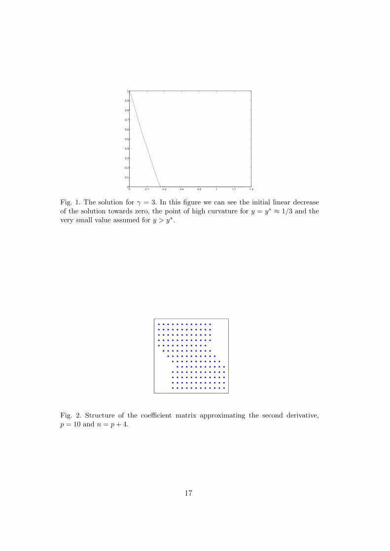
A plot of the solution θ(y) of (3)–(5) for γ = 3 is given in Figure 1. In thisplot we can see that for smaller values of y the solution θ(y) decreases almostlinearly, coming close to zero at the point y ≈ 1/γ. As θ approaches zero itfollows from (3)–(5) that θyy increases. Indeed, we can see from the figure thatthe solution has high positive curvature close to this point. For larger valuesof y the solution asymptotes to a constant value so that

θ(y) → θ∞ as y → ∞.

Of interest are both θ∞ and the point y∗ (a rescaling of the wetting front x∗)at which θyy takes its maximum value, so that

θyyy(y∗) = 0. (6)

In analogy to the time-dependent problem we will refer to the latter as thewetting front. Indeed, if y < y∗ then θ = O(1) and if y > y∗ then θ = O(e−γ

2).

An asymptotic study of this problem for large values of γ is given in [9], theresults of which are summarised in Section 1. One purpose of this paper isto use an accurate high order numerical method to examine the asymptoticpredictions of the latter paper and to accurately determine both the locationof the wetting front and the value of θ∞.

This problem poses a significant numerical challenge. Whilst the error terms inthe asymptotic expansions (say of y∗) decay polynomially in γ as γ increases,it is shown in [9] that the curvature and final value are exponential in γ, thatis

θyy(y∗) ∼ eγ

2

and θ∞ ∼ e−γ2

.

Hence, for even moderately large values of γ we see that the solution featuresa near-singularity in its higher derivatives, and moreover the solution is almostidentically equal to 0 for larger values of y. Indeed in the calculations reportedin this paper we have values of θyy ∼ 10138 and θ∞ ∼ 10−141. Conventionalinitial value solvers such as the Gear solvers in the MATLAB routine ode15s

3

are unable to deal with the form of these singularities for values of γ at whichthe asymptotic results are expected to become sharp (for example values ofγ > 10). For the larger values of γ required to study the asymptotic resultsa different numerical approach is required, and it is the difficulties describedabove that put this problem in the focus of the higher order methods that wewill discuss in this paper. The numerical challenge is thus to find discretizationschemes and adaptive mesh selection methods which are robust with respectto the dramatic variation in the stepsizes (up to 140 orders of magnitude in ourcomputations reported below) which may be expected due to the predictedsolution behavior as the curvature of θ rapidly increases. Earlier attempts inthis direction have not been fully satisfactory, as the problem could only besolved for values of γ remote from the asymptotical regime [9].

Accordingly, in this paper we propose the construction of a variable step sizenumerical scheme directly for the second order problem (3)–(5) without re-sorting to a transformation to first order form. The idea of discretizing eachderivative of the second order continuous problem by means of finite differenceschemes has been largely considered in the past, in particular in the numericalsolution of partial differential equations using schemes of low order (and withsmall stencils). In [4] and later in [1,3,5] it was proposed to apply high orderfinite difference schemes for the solution of boundary value problems for or-dinary differential equations by considering different formulae with the sameorder in the initial and final points of the grid, following the idea inherited byboundary value methods (BVM) [7]. One major advantage of this approach isassociated with the fact that the vector of unknowns contains only the solutionof the problem. This choice, on the one hand, reduces the computational costof the algorithm with respect to the standard approaches which transform thesecond order equation into a first order one containing both the solution andits first derivative as unknowns. On the other hand, it simplifies the stepsizevariation and allows the solution of fully implicit problems without any changein the approach. Moreover, in [14] it was demonstrated that a solution in thesecond order formulation may yield an advantage with respect to the condi-tioning of the linear systems of equations associated with the discretizationscheme. Also, it is clear that in this approach, only the smoothness of the so-lution, but not of its derivative, affects the step-size selection process, see [10].Finally, in the original formulation there is complete freedom in the choice ofthe schemes approximating each derivative which could not only depend onwhether an initial or boundary value problem is solved, but also on the prob-lem data and the discretization points. In [2] the same idea is applied to IVPsfor ODEs. Two approaches are proposed to take care of the first derivativein the initial point: we can choose to approximate this initial condition bymeans of an appropriate formula or to define difference schemes which makeuse of the analytical first derivative in the first point. As a general belief, thesecond approach seems to be preferable but, for the problem (3)–(4) the firststrategy is used, since the solution’s derivative may be quite different from

4

the solution itself (and hence affect the stepsize variation). The computationswhich enable to provide the mentioned results are only possible due to thishighly flexible, adaptive finite difference method which is able to cope withextremely unsmooth step-size sequences. The numerical method is sufficientlygood to not only confirm the asymptotical calculations in [9] but to also give aclear indication of the structure of further terms, which are currently beyondthe reach of theoretical analysis.

The layout of the remainder of this paper is as follows. The numerical methodis described in Section 2. Asymptotical solution properties are studied in Sec-tion 3. In Section 3.1, we briefly describe the asymptotic theory for (3)–(5)given in [9] and compare the results with our numerical simulations for val-ues of γ ≤ 18, for which θyy(y

∗) ≈ 10138 and θ∞ ≈ 10−141. In Section 3.2 adetailed analysis of the solution behaviour is given in the so-called mid-rangeof the independent variable in which y ≈ y∗ and θyy(y) has very high values.We compare directly the asymptotical and numerical profiles. In Section 4 weshow the form of the solution θ(y) and give plots of the solution and of itsderivatives to illustrate the nature of the numerical difficulties and resultingerrors described above. Finally in Section 5 we draw some conclusions fromthis work.

2 The Numerical Method

Here we describe the finite difference schemes underlying the computationspresented in this manuscript. The coefficients in these multistep methods areconstructed via Taylor expansion such as to yield high-order approximations.The particular strength is the robustness with respect to large variations inthe step-sizes close to the point of high curvature, which result from an adap-tive procedure based on local error estimates computed by mesh halving. Themethods are applied to second-order initial value problems in their originalformulation, and use different formulae for the appearing derivatives. The dif-ference formulae are defined for equidistant grids and used on small subinter-vals of the time domain. Stepsize variation is performed after each subintervalas in the general block–BVM framework [7].

For the sake of clarity we consider the numerical solution of a general secondorder initial value problem

f(y, θ, θy, θyy) = 0,

θ(y0) = θ0, θy(y0) = θy,0.(7)

We first specify an initial stepsize h0 and a grid of equispaced points Y =[y0, y1, . . . , yn], yi = y0 + ih0. Denote the corresponding numerical approxima-

5

tion by

Θ = [θ0, θ1, . . . , θn].

Following the idea in [2,4,5], we discretize separately the derivatives in (7) bymeans of suitable high order finite difference schemes

θy(yi) ≃1

h

r∑

j=−s

a(s)s+jθi+j =: θy,i, (8a)

θyy(yi) ≃1

h2

r∑

j=−s

c(s)s+jθi+j =: θyy,i, (8b)

where a(s)s+j, c

(s)s+j are the coefficients of the methods which are fixed in order to

reach the maximally possible order of accuracy. The integers s and r representthe number of left and right values required to approximate θy(yi) and θyy(yi),and are strictly related to the order and the stability of the formula. For thisproblem we choose, when possible, r = s obtaining formulae (called ECDFin [5]) of even order p = 2s for both the first and the second derivative. Forexample, we have for

Order 4

h2 θyy(yi) ≈ − 112θi−2 +

43θi−1 −

52θi +

43θi+1 −

112θi+2,

h θy(yi) ≈112θi−2 −

23θi−1 +

23θi+1 −

112θi+2,

Order 6

h2 θyy(yi) ≈190θi−3 −

320θi−2 +

32θi−1 −

4918θi +

32θi+1 −

320θi+2 +

190θi+3,

h θy(yi) ≈ − 160θi−3 +

320θi−2 −

34θi−1 +

34θi+1 −

320θi+2 +

160θi+3.

We observe that the coefficients are symmetric and skew-symmetric for the sec-ond and first derivatives, respectively. We have successfully used these schemesup to the order 10.

We compute the unknowns in Θ by solving the nonlinear system

f(yi, θi, θy,i, θyy,i) = 0, i = 1, . . . , n− 1, (9)

together with the initial conditions. Since the above symmetric formulae oforder p > 2 cannot be used to approximate θy(yi) and θyy(yi), i = 1, . . . , p/2−1and i = n− p/2 + 1, . . . , n− 1, schemes of the form (8) with different stencils(but the same order) must be provided at the beginning and the end of thegrid. We call them initial and final formulae (see [7]). Examples of the initial

6

schemes are

Order 4

h2 θyy(y1) ≈5

6θ0 −

5

4θ1 −

1

3θ2 +

7

6θ3 −

1

2θ4 +

1

12θ5,

h θy(y1) ≈ −1

4θ0 −

5

6θ1 +

3

2θ2 −

1

2θ3 +

1

12θ4.

Order 6

h2 θyy(y1) ≈7

10θ0 −

7

18θ1 −

27

10θ2 +

19

4θ3 −

67

18θ4 +

9

5θ5 −

1

2θ6 +

11

180θ7,

h2 θyy(y2) ≈ −11

180θ0 +

107

90θ1 −

21

10θ2 +

13

18θ3 +

17

36θ4 −

3

10θ5 +

4

45θ6 −

1

90θ7,

h θy(y1) ≈ −1

6θ0 −

77

60θ1 +

5

2θ2 −

5

3θ3 +

5

6θ4 −

1

4θ5 +

1

30θ6,

h θy(y2) ≈1

30θ0 −

2

5θ1 −

7

12θ2 +

4

3θ3 −

1

2θ4 +

2

15θ5 −

1

60θ6.

The final schemes used to approximate θy(yn), θyy(yn) and, for the order 6,θy(yn−1), θyy(yn−1), are not reported. Anyway, the coefficients of these meth-ods correspond to the initial ones given above, but in reversed order and withthe opposite sign in case of the first derivative. Note that for the second deriva-tive, the order of the initial methods is p = r + s− 1 (we need one additionalvalue to obtain the required order).

The number of grid points n ≥ p computed by solving (9) is linked to stabilityand computational cost. Larger n means better stability properties but highercomputational cost [2,7]. For this problem we have fixed n = p + 4. Thestructure of the coefficient matrix associated with the second derivative forp = 10 is shown in Figure 2. In this example, the main scheme is appliedfive times and combined with four initial and final schemes. The size of theresulting matrix is (n − 1) × (n + 1), but the first column can be neglectedbecause the starting value θ0 is known. To complete the discretization, θy(y0)is approximated by a suitable starting scheme obtained by choosing s = 0 in(8). Examples of these latter formulae are:

Order 4:

hθy(y0) ≈ −2512θ0 + 4θ1 − 3θ2 +

43θ3 −

14θ4,

Order 6:

hθy(y0) ≈ −4920θ0 + 6θ1 −

152θ2 +

203θ3 −

154θ4 +

65θ5 −

16θ6.

7

Once the solution in yi = y0 + ih0, i = 1, . . . , n, has been approximated, thestepsize is changed according to an estimate of the local relative error basedon the mesh halving strategy and the algorithm is iterated on a subsequentsubinterval. The code uses a classical time stepping strategy [19] with safetyfactor 0.7

hnew =

(

0.7 tol

error

)1

(p+1)

hold.

In order to obtain the numerical approximations, for all the even orders from4 to 10 we have used initial stepsize h0 = 1e− 3 and relative error tolerancetol = 1e − 12 for both the solution and the Newton iteration. Moreover, westress that the numerical solution is reliable having the computed stepsize thesame order of magnitude of the solution and of its derivative.

Since however the second last values θ(yn−1) and θy(yn−1) are better approxi-mated than θ(yn) and θy(yn), we discard the last value in Θ, use formula (8)with i = n− 1, r = 1 to compute θy,n−1, and continue the algorithm with theinitial conditions [θn−1, θy,n−1].

3 Asymptotic Solution Properties

3.1 Asymptotics for Large γ

In this section we outline the main asymptotic predictions for the solutions of(3)–(5) which are presented in [9] and will show how these are supported bythe numerical calculations. In [9] a matched asymptotic expansion method isused to find an asymptotic form of both the wetting front y∗ defined in (6)as the point of maximal curvature and the final value of log(θ∞), expressingboth as formal asymptotic series expanded in powers of 1/γ with γ ≫ 1. Theasymptotic series are found by matching descriptions of the solution in aninner range with y < y∗ ≈ 1/γ, a mid-range with y ≈ y∗ and an outer rangewith y ≫ y∗. It is in the mid-range where the most delicate behaviour occurs,with exponentially large (in γ) values for θyy making the asymptotic theorychallenging in this case. We will describe the precise form of the solution inthe mid-range in Section 3.2.

In [9] it is proposed that as γ → ∞ the value of θ(1/γ) is given asymptoticallyby the expression

θ

(

1

γ

)

=1

2γ2−

log(γ)

γ4+

b

γ4, (10)

8

where

b = b∗ +O

(

1

γ2

)

with b∗ =11

12−

1

2log(2) ≈ 0.57009307.... (11)

Similarly, the final value θ∞ satisfies the asymptotic relation

log(θ∞) = −γ2 −1

2+α

γ2, (12)

where it is conjectured that α takes the form

α = α∗ +O

(

1

γ2

)

, (13)

with α∗ an unknown constant. Furthermore, the location of the wetting fronty∗ is given asymptotically by the expression

y∗ =1

γ+

1

2γ3+β

γ5, (14)

where

β = β∗ +O

(

1

γ2

)

, with β∗ =11

12. (15)

At the wetting front we have

θ(y∗) ≈ eθ∞ and θyy(y∗) ≈

eγ2−1/2

γ2=: θyy. (16)

Using the finite difference schemes described in the previous section, we studythese asymptotic results by solving the initial value problem (3)–(5) for γ =2, 3, . . . 18. For γ > 18 the solution for large y where θ ≈ θ∞ = 10−141 ∼ e−γ

2

is too small to be computed accurately and for γ > 26 it is smaller than thesmallest positive double precision machine number. Note that although γ = 18poses a serious challenge for the numerical method, the predicted asymptoticerror of order 1/γ2 is not unreasonably small. We considered methods of or-ders p = 4, 6, 8, and 10 to understand how the order of the numerical methodinfluences the accuracy of the approximate solutions. For the purpose of illus-tration, we will generally give the results for p = 4 and p = 8. As a generalremark, we observe that the discretization errors are larger than the round-offerrors of the floating point operations. Moreover, we propagate the solutionusing variable stepsizes, and for a fixed tolerance, methods of higher orderallow for larger stepsizes but they do not necessarily achieve better precision.This is most probably due to the fact that higher derivatives of the solution θare extremely unsmooth. The solution has been computed on finite intervals[0, y∞], with the interval endpoint y∞ = 10, 20, 30, 40, 50, to see how stronglythe value of θ(y∞) depends on the length of the interval of integration. It turns

9

out that, especially for large values of γ, the influence of the interval length isnegligible. Therefore, from now on, we use the interval [0, 10] and θ∞ ≈ θ(10)for all calculations.

In Table 1 we present the results of the numerical computations of the variousterms in the expressions above. All data are given for computations withγ = 10 and γ = 18, respectively. Since the reference values are asymptoticallycorrect for large values of γ, we expect to observe higher accuracy for largerγ. In rows 1 and 2 of Table 1, we specify the values of θ∞ and y∗, where y∗

is defined to be the point where the numerically computed value of θyy takesits maximal value in the interval [0, y∞] = [0, 10]. In row 3 we first reportthe relative error in approximating − log(θ∞) by γ2 + 1

2and then in row 4

we compute an approximation for α as defined in (12). The values in row 3confirm that the value of θ∞ has been computed accurately (the relative erroris always smaller than γ−4) and the computed value for α in expression (12)is α ≈ −0.08.

Motivated by the relation (14) we define

s∗ = γ3y∗ − γ2 =1

2+O

(

1

γ2

)

. (17)

In row 5 of Table 1 we specify the relative error |s∗ − 0.5|/0.5 and in row 6we use (14) to approximate the value of β. Again the relative error is smallerthan γ−2 while the value of β is close to 0.95.

Rows 7 and 8 contain the numerical approximations of θ(y∗) and θyy(y∗),

showing the very rapid increase in the value of the latter with γ. In rows 9and 10 we specify the relative errors

|θ(y∗)− eθ∞|

eθ∞, and

∣

∣

∣θyy(y∗)− θyy

∣

∣

∣

θyy, (18)

where θ(y∗) and θyy(y∗) denote our numerically obtained values. Finally, rows

11 and 12 contain the numerical value of b as given in (10) and the relativeerror. In all of these expressions the relative error decreases as γ increases,demonstrating that to leading order both the numerical and asymptotic cal-culations are correct.

Given the relatively modest values of γ used in the computations, and thecorresponding large asymptotic errors, it is necessary to post-process the nu-merical results to determine the finer structure of the solution and to verifythe accuracy of the methods used. This post-processing allows us to makesome further conjectures about the asymptotic solution. Taking the asymp-totic expressions for α, β and b in expressions (10), (12), and (14) in the preciseform

10

α = α∗ +A

γ2, (19)

β = β∗ +B

γ2, (20)

b = b∗ +C

γ2, (21)

we substitute the results from Table 1 for γ = 10 and γ = 18 to find thecorresponding values of α∗, β∗, b∗, A, B, C. This calculation gives

α∗ ≈ −0.0834 ≈ −1.0004/12, with A ≈ −0.089,

β∗ ≈ 0.9163 ≈ 10.9954/12, with B ≈ 2.96,

b∗ ≈ 0.5620 with C ≈ 4.81.

These results are close to the asymptotical results given in (15), (11) for whichβ∗ = 11/12 ≈ 0.9166666, and b∗ ≈ 0.57009, while the result for α∗ stronglyimplies the new result that

α∗ = −1

12. (22)

We conclude from this numerical calculation that there is strong evidence forthe correctness of the asymptotic expressions in [9] and that the wetting fronty∗ is located at the point

y∗ ≈1

γ+

1

2γ3+

11

12γ5+

2.96

γ7.

Moreover,

log(θ∞) ≈ −γ2 −1

2−

1

12γ2−

0.089

γ4.

3.2 Mid–range Calculation — Asymptotics and Numerical Results

Next, we consider the asymptotical solution properties in the regime wherey lies in the mid-range close to y∗ ≈ 1/γ. In this very delicate region wherethe solution changes rapidly, we compare the asymptotic form of the functionwith the numerical profiles. It is convenient to rescale both the dependent andindependent variables in this region according to (17), such that

y =1

γ+

s

γ3and v(s) = γ4θ(y),

with |s| varying between 1 and γ2.

We first discuss the case of negative s.

11

Table 1Asymptotic results.

γ = 10

Order 4 8

θ∞ 2.254440321030590e−44 2.254439903035485e−44

y∗ 1.005094588206025e−01 1.005094588173695e−01

| log(θ∞) + γ2 + 0.5|

γ2 + 0.58.381534862525284e−06 8.383379735339227e−06

α −8.423442536837911e−02 −8.425296634015922e−02

|s∗ − 0.5|/0.5 1.891764120503581e−02 1.891763473901165e−02

β 9.458820602506902e−01 9.458817369495821e−01

θ(y∗) 6.126853837541197e−44 6.179228381160976e−44

θyy(y∗) 1.648468426869335e+41 1.648412414631253e+41

|θ(y∗)− eθ∞|

eθ∞2.203452148159067e−04 8.326316736789704e−03

|θyy(y∗)− θyy|/θyy 1.106641417450169e−02 1.103205980544998e−02

b 5.138760976981811e−01 5.138757975462900e−01

|b− b|/b 9.861017615723677e−02 9.861070265352932e−02

γ = 18

Order 4 8

θ∞ 1.178498689884995e−141 1.178497239286140e−141

y∗ 5.564177918914028e−02 5.564177918834908e−02

| log(θ∞) + γ2 + 0.5|

γ2 + 0.57.913110850624213e−07 7.951042681243711e−07

α −8.319686486129285e−02 −8.359567254206013e−02

|s∗ − 0.5|/0.5 5.712462132123619e−03 5.712452903708254e−03

β 9.254188654173835e−01 9.254173704034648e−01

θ(y∗) 3.198906899145607e−141 3.211721064871286e−141

θyy(y∗) 9.664468728333972e+137 9.664458760222388e+137

|θ(y∗)− eθ∞|

eθ∞1.431149209001307e−03 2.570147096053791e−03

|θyy(y∗)− θyy|/θyy 3.363040886020695e−03 3.362005998844594e−03

b 5.471501619326116e−01 5.471487116780027e−01

|b− b|/b 4.024415556753806e−02 4.024669945847258e−02

12

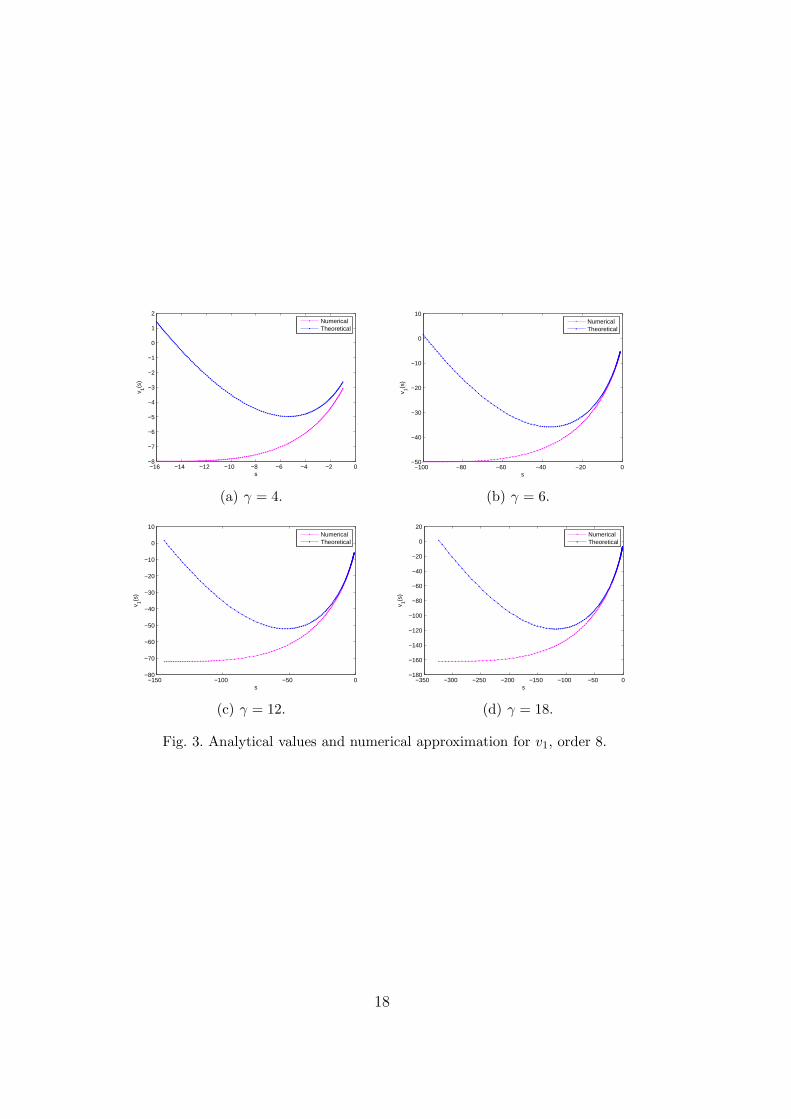
Case 1: Let −γ2 ≪ s≪ −1. In [9] an asymptotic series for the function v(s)is developed in the form

v(s) = γ2v0(s) + v1(s) +O

(

1

γ2

)

. (23)

A careful application of the method of matched asymptotic expansions thenimplies that

v0(s) =1

2− s (24)

and

v1(s) = 2 log(γ)s− log(γ) + b−(

s−1

2

)

log(

1

2− s

)

+log(2)

2, (25)

where b =11

12−

1

2log(2).

In Figures 3 and 4, we plot the values of v1(s) and their numerical approx-imations together with the relative errors (logarithmic scale), respectively.Computations were realized with the method of order 8. We can see the de-sired behaviour in the asymptotical regime −γ2 ≪ s < 0. Note furthermorethat as expected the approximation improves as γ increases.

We next consider the mid-range with positive values of s. It is in this rangethat we see the rapid transition from polynomial to exponential decay.

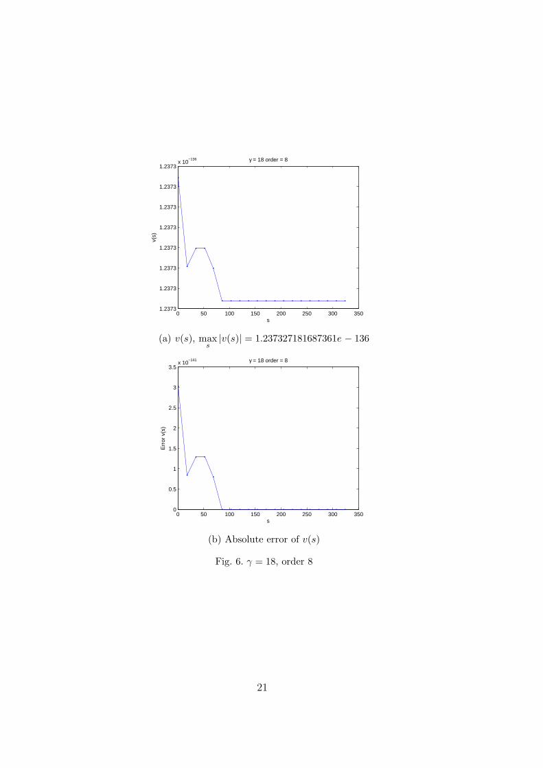
Case 2: Let 1 ≪ s≪ γ2. The asymptotic form of v(s) is given by [9],

v(s) = v∞(

1 + e−γee−(s−s∗)/v∞)

, (26)

where s∗ = 12+ O(1/γ2) and γe ≈ 0.577215665 is the Euler–Mascheroni con-

stant. For a large value of γ the value of v∞ is very small, and therefore, v(s)in (26) is constant and coincides with v∞ ≡ θ∞/γ

4.

Figures 5 and 6 show the graphs of v(s) and their absolute errors obtainedbased on (26), computed by the method of order 8 for γ = 10 and γ = 18,respectively. Note that in spite of the small solution values, the numericalresults are still meaningful with an accuracy of about five digits. However, thevery small value of the solution makes all comparisons difficult.

4 Accuracy of the Numerical Method

Finally, we demonstrate the numerical challenges and the resulting numericalerrors encountered in the course of the computations which led to the results

13

on the asymptotical solution behavior discussed in the previous sections. Forlarger values of γ, the solution features an interface with very large values ofthe second derivative. This can only be resolved with an adaptive step selectionprocedure which allows for extreme step-size variations without jeopardizingthe stability of the computations.

In Figure 7, we show the graphs in a logarithmic scale of the numerical solutionand its first and second derivatives for the value γ = 18 computed by thenumerical method of order 8. The rapid change in θ and its derivatives closeto the wetting front is very clear from these figures. It was found that theapproximation of the first and the second derivative becomes unreliable inthe area where the solution becomes constant. In fact, since derivatives arecomputed by means of linear combinations of the solution values (using finitedifference formulae (8)), it is really unlikely that they can be lower (in absolutevalue) than θ∞EPS, where EPS is the machine precision, and in this case mustbe treated as 0.

Secondly, in Figure 8 we plot the variation of the stepsizes for the methodsof orders 4, 6, 8, and 10. The used tolerance is 1e−12 and the initial stepsize is 1e−3. We note that the orders 6 and 8 require the smallest number ofmeshpoints, since the size of each block is p+ 4. 1 We observe the very smallstepsizes used in these methods close to the point of high curvature. Note thatthe same minimal stepsize is defined for all orders, and this stepsize is reachedwith fewer but larger steps if the order of the method is higher.

5 Conclusions

We have discussed the numerical solution of a second-order ODE problemwhich arises as a model of flow through porous media. The solution of thisproblem features an interface with very large values of the higher derivatives.An adaptive finite difference method is employed to approximate the solutionnumerically and verify predictions derived by asymptotic theory.

The numerical investigation is successful. The solution algorithm can cope witha large variation in the stepsizes and thus can serve to accurately approximatethe location of the interface and asymptotic characteristics of the solution.

In particular for the case where the interface is very sharp (blow-up of thesecond derivative), the simulations give very stable results which closely matchthe theoretical results, both in confirming certain of the asymptotic predictions

1 Clearly, the number of meshpoints is equal to p + 4 times the number of blocks(see Section 2).

14

for the location of the interface and the asymptotic value at infinity derived in[9] and also in giving strong evidence for further asymptotic results which arebeyond the existing theory. This lends validity to both the numerical methodand the asymptotic calculation.

Thus the asymptotic results and the numerical procedures are both verified,parameters not given by the a priori analysis are determined and new predic-tions about the solution structure are indicated.

Acknowledgment

We thank EU FP7 Marie Curie ITN FIRST for partly supporting this work.Moreover we would like to thank the referee for helpful and detailed commentson the presentation of the material in this manuscript, which have been a greathelp in improving the paper.

References

[1] P. Amodio and G. Settanni. Variable step/order generalized upwind methodsfor the numerical solution of second order singular perturbation problems.JNAIAM J. Numer. Anal. Indust. Appl. Math., 4:65–76, 2009.

[2] P. Amodio and G. Settanni. High order finite difference schemes for the solutionof second order initial value problems. JNAIAM J. Numer. Anal. Indust. Appl.Math., 5:3–16, 2010.

[3] P. Amodio and G. Settanni, A finite differences MATLAB code for thenumerical solution of second order singular perturbation problems. J. Comput.Appl. Math. 236:3869–3879, 2012.

[4] P. Amodio and I. Sgura. High-order finite difference schemes for the solutionof second-order BVPs. J. Comput. Appl. Math., 176:59–76, 2005.

[5] P. Amodio and I. Sgura. High order generalized upwind schemes and numericalsolution of singular perturbation problems. BIT, 47:241–257, 2007.

[6] D.K. Babu. Infiltration analysis and perturbation methods. 1. Absorption withexponential diffusivity. Water Resour. Res., 12:89–93, 1976.

[7] L. Brugnano and D. Trigiante. Solving Differential Problems by MultistepInitial and Boundary Value Methods. Gordon and Breach Science Publishers,Amsterdam, 1998.

[8] W. Brutsaert. Universal constants for scaling the exponential soil waterdiffusivity. Water Resour. Res., 15(2):481–483, 1979.

15

[9] C.J. Budd and J. Stockie. Asymptotic behaviour of wetting fronts in porousmedia with exponential moisture diffusivity. Submitted, 2013.

[10] J. Cash, G. Kitzhofer, O. Koch, G. Moore, and E.B. Weinmuller. Numericalsolution of singular two-point BVPs. JNAIAM J. Numer. Anal. Indust. Appl.Math., 4:129–149, 2009.

[11] Z. Chen, G. Huan, and Y. Ma. Computational Methods for Multiphase Flowsin Porous Media. SIAM, Philadelphia, PA, 2006.

[12] B. E. Clothier and I. White. Measurement of sorptivity and soil water diffusivityin the field. Soil Sci. Soc. Amer. J., 45:241–245, 1981.

[13] J. Crank. The Mathematics of Diffusion. Oxford University Press, Oxford,U.K., 1975.

[14] G. Kitzhofer, O. Koch, P. Lima, and E.B. Weinmuller. Efficient numericalsolution of the density profile equation in hydrodynamics. J. Sci. Comput.,32:411–424, 2007.

[15] C. Leech, D. Lockington, and P. Dux. Unsaturated diffusivity functions forconcrete derived from NMR images. Mater. Constr., 34:413–418, 2003.

[16] J.-Y. Parlange. A note on a three-parameter soil–water diffusivity function —Application to the horizontal infiltration of water. Soil Sci. Soc. Amer. J.,37:318–319, 1973.

[17] M.B. Parlange, S.N. Prasad, J.-Y. Parlange, and M.J.M. Romkens. Extensionof the Heaslet–Alksne technique to arbitrary soil water diffusivities. WaterResour. Res., 28:2793–2797, 1992.

[18] J.D. Parslow, D. Lockington, and J.-Y. Parlange. A new perturbation expansionfor horizontal infiltration and sorptivity estimates. Transp. Porous Media,3:133–144, 1988.

[19] W.H. Press, B.P. Flannery, S.A. Teukolsky, and W.T. Vetterling. NumericalRecipes in C — The Art of Scientific Computing. Cambridge University Press,Cambridge, U.K., 1988.

[20] M. Rose. Numerical methods for flows through porous media I. Math. Comp.,40(162):435–467, 1983.

16

0 0.2 0.4 0.6 0.8 1 1.2 1.40

0.1

0.2

0.3

0.4

0.5

0.6

0.7

0.8

0.9

1

Fig. 1. The solution for γ = 3. In this figure we can see the initial linear decreaseof the solution towards zero, the point of high curvature for y = y∗ ≈ 1/3 and thevery small value assumed for y > y∗.

Fig. 2. Structure of the coefficient matrix approximating the second derivative,p = 10 and n = p+ 4.

17

−16 −14 −12 −10 −8 −6 −4 −2 0−8

−7

−6

−5

−4

−3

−2

−1

0

1

2

s

v 1(s)

NumericalTheoretical

(a) γ = 4.

−100 −80 −60 −40 −20 0−50

−40

−30

−20

−10

0

10

s

v 1(s)

NumericalTheoretical

(b) γ = 6.

−150 −100 −50 0−80

−70

−60

−50

−40

−30

−20

−10

0

10

s

v 1(s)

NumericalTheoretical

(c) γ = 12.

−350 −300 −250 −200 −150 −100 −50 0−180

−160

−140

−120

−100

−80

−60

−40

−20

0

20

s

v 1(s)

NumericalTheoretical

(d) γ = 18.

Fig. 3. Analytical values and numerical approximation for v1, order 8.

18

−16 −14 −12 −10 −8 −6 −4 −2 010

−1

100

101

102

103

s

Err

or

(a) γ = 4.

−100 −80 −60 −40 −20 010

−2

10−1

100

101

102

103

s

Err

or

(b) γ = 10.

−150 −100 −50 010

−2

10−1

100

101

102

103

s

Err

or

(c) γ = 12.

−350 −300 −250 −200 −150 −100 −50 010

−3

10−2

10−1

100

101

102

103

s

Err

or

(d) γ = 18.

Fig. 4. Relative error of v1, order 8.

19

0 20 40 60 80 1002.2545

2.2545

2.2545

2.2545

2.2545

2.2545x 10

−40 γ = 10 order = 8

s

v(s)

(a) v(s), maxs

|v(s)| = 2.254510924061732e − 040

0 20 40 60 80 1000

0.5

1

1.5

2x 10

−45 γ = 10 order = 8

s

Err

or v

(s)

(b) Absolute error of v(s)

Fig. 5. γ = 10, order 8

20

0 50 100 150 200 250 300 3501.2373

1.2373

1.2373

1.2373

1.2373

1.2373

1.2373

1.2373x 10

−136 γ = 18 order = 8

s

v(s)

(a) v(s), maxs

|v(s)| = 1.237327181687361e − 136

0 50 100 150 200 250 300 3500

0.5

1

1.5

2

2.5

3

3.5x 10

−141 γ = 18 order = 8

s

Err

or v

(s)

(b) Absolute error of v(s)

Fig. 6. γ = 18, order 8

21

10−4

10−3

10−2

10−1

100

101

10−150

10−100

10−50

100

y

θ(y)

(a) Numerical solution.

10−4

10−3

10−2

10−1

100

101

10−200

10−150

10−100

10−50

100

1050

y

θ’(y

)

(b) Numerical approximation of minus the first derivative.

10−4

10−3

10−2

10−1

100

101

10−200

10−100

100

10100

10200

y

θ’’(y

)

(c) Numerical approximation of the second derivative.

Fig. 7. Solution and its derivatives for γ = 18. Missing points correspond to negativevalues of −θy(y) and θyy(y)

22

0 1000 2000 3000 4000 5000 6000 7000 800010

−150

10−100

10−50

100

Number of blocks

Ste

p si

ze

(a) order = 4.

0 500 1000 1500 2000 250010

−150

10−100

10−50

100

Number of blocks

Ste

p si

ze

(b) order = 6.

0 200 400 600 800 1000 1200 1400 160010

−150

10−100

10−50

100

Number of blocks

Ste

p si

ze

(c) order = 8.

0 200 400 600 800 1000 1200 1400 1600 180010

−150

10−100

10−50

100

Number of blocks

Ste

p si

ze

(d) order = 10.

Fig. 8. Step size variation for each block, γ = 18.

23