UNCLASSIFIED

Asymptotic Distribution of Rewards Accumulated by

Alternating Renewal Processes

Patrick Chisan Hew

Joint and Operations Analysis Division

Defence Science and Technology Group

DST-Group�TN�1631

ABSTRACT

This technical note considers processes that alternate randomly between `working' and `broken'over an interval of time. Suppose that the process is rewarded whenever it is `working', at arate that can vary during the time interval but is known completely. We prove that if the timeinterval is long then the accumulated reward is approximately normally distributed and theapproximation becomes perfect as the interval becomes in�nitely long. Moreover we calculatethe means and variances of those normal distributions. Formally, consider an alternatingrenewal process on the states `working' vs `broken'. Suppose that during any interval [0, τ ],the process is rewarded at rate g(t/τ) if it is working at time t. Let Qτ be the reward that isaccumulated during [0, τ ]. We calculate µQτ and σ2Qτ such that (Qτ − µQτ )/σQτ converges indistribution to a standard normal distribution as τ →∞.

RELEASE LIMITATION

Approved for Public Release

UNCLASSIFIED

UNCLASSIFIED

Produced by

Joint and Operations Analysis Division506 Lorimer St,Fishermans Bend, Victoria 3207, Australia

Telephone: 1300 333 362

c© Commonwealth of Australia 2017October 2017

APPROVED FOR PUBLIC RELEASE

UNCLASSIFIED

AR-016-866

UNCLASSIFIED

Asymptotic Distribution of Rewards Accumulated by

Alternating Renewal Processes

Executive Summary

This technical note documents some research into processes that alternate randomly between`working' and `broken' over an interval of time. It supposes that the process is rewardedwhenever it is `working', at a rate that can vary during the time interval but is known com-pletely. We study the reward that is accumulated over that time interval. For example,consider a solar panel that can earn money if it is exposed to the sun, at a rate of 5 dollarsper hour before noon and 10 dollars per hour after noon. What is the amount of money thatit will earn over a given 24 hour period?

The key �nding is that if the time interval is long then the accumulated reward is approximatelynormally distributed, and the approximation becomes perfect as the interval becomes in�nitelylong. The research also calculates the means and variances of those normal distributions. Thevalues are obtained from the rates at which the process is rewarded when working (the dollarsper hour in the example given above), and statistics about the times to failure and times torepair (the durations to go from working to broken and from broken to working).

This technical note is the expanded version of an article that was prepared for the journalStatistics & Probability Letters [Hew 2017]. It provides the details of the proofs that wereabridged for the journal article. The research was motivated by studies of a number of militaryoperations. When collapsed to their essentials, the operations could be modelled in terms ofa sensor that alternates randomly between working and broken, and is looking for a targetthat reluctantly gives away glimpses at random times. Consider in particular the probabilityof seeing the k-th glimpse. Intuitively, at any time, the glimpse provides some probability ofbeing detected if the sensor is working at that time. The probability of seeing the glimpse isthe accumulation of those probabilities over the time interval. Hence by using the resultsin this article, we know that the probability of seeing the k-th glimpse is approximatelynormally distributed, and we can use that knowledge to make predictions about operationalperformance. Full details will be reported separately.

UNCLASSIFIED

UNCLASSIFIED

This page is intentionally blank

UNCLASSIFIED

UNCLASSIFIED

Contents

1 INTRODUCTION. . . . . . . . . . . . . . . . . . . . . . . . . . . . . . . . . . . . . . . . . . . . . . . . . . . . . . . . . . . . . . . . . . . . . . . . . . . . 1

2 PRELIMINARIES . . . . . . . . . . . . . . . . . . . . . . . . . . . . . . . . . . . . . . . . . . . . . . . . . . . . . . . . . . . . . . . . . . . . . . . . . . . 2

3 PROOF OF MAIN RESULT . . . . . . . . . . . . . . . . . . . . . . . . . . . . . . . . . . . . . . . . . . . . . . . . . . . . . . . . . . . . . . 43.1 Proof of Proposition 1 . . . . . . . . . . . . . . . . . . . . . . . . . . . . . . . . . . . . . . . . . . . . . . . . . . . . . . . . . . . . . . . . . 63.2 Proof of Proposition 2 . . . . . . . . . . . . . . . . . . . . . . . . . . . . . . . . . . . . . . . . . . . . . . . . . . . . . . . . . . . . . . . . . 63.3 Proof of Proposition 3 . . . . . . . . . . . . . . . . . . . . . . . . . . . . . . . . . . . . . . . . . . . . . . . . . . . . . . . . . . . . . . . . . 73.4 Proof of Proposition 4 . . . . . . . . . . . . . . . . . . . . . . . . . . . . . . . . . . . . . . . . . . . . . . . . . . . . . . . . . . . . . . . . . 10

4 REMARKS . . . . . . . . . . . . . . . . . . . . . . . . . . . . . . . . . . . . . . . . . . . . . . . . . . . . . . . . . . . . . . . . . . . . . . . . . . . . . . . . . . . . 11

5 ACKNOWLEDGEMENTS . . . . . . . . . . . . . . . . . . . . . . . . . . . . . . . . . . . . . . . . . . . . . . . . . . . . . . . . . . . . . . . . . 13

6 REFERENCES . . . . . . . . . . . . . . . . . . . . . . . . . . . . . . . . . . . . . . . . . . . . . . . . . . . . . . . . . . . . . . . . . . . . . . . . . . . . . . . . 13

APPENDIX A: THE VARIANCE OF ASYMPTOTICALLY NORMAL SUMS

OF STRICTLY STATIONARY PROCESSES UNDER WEIGHTING. . . . . . . . . . 15A.1 Proofs . . . . . . . . . . . . . . . . . . . . . . . . . . . . . . . . . . . . . . . . . . . . . . . . . . . . . . . . . . . . . . . . . . . . . . . . . . . . . . . . . . . . . 15A.2 Remarks . . . . . . . . . . . . . . . . . . . . . . . . . . . . . . . . . . . . . . . . . . . . . . . . . . . . . . . . . . . . . . . . . . . . . . . . . . . . . . . . . . 18

UNCLASSIFIED

UNCLASSIFIED

This page is intentionally blank

UNCLASSIFIED

UNCLASSIFIED

DST-Group�TN�1631

1. Introduction

Consider a stochastic process Xt that at any given time t is either `working' or `broken',and where the process has the renewal property � a so-called alternating renewal process. Indetail, the process consists of a sequence of durationsW1, B1, W2, B2, . . . where each durationworking Wk is followed by a duration broken Bk and the process renews at the start of eachworking duration. We suppose that over an interval of time [0, τ ], the process is rewarded atrate g(t/τ) if it is working at time t where g is a real-valued function on the interval [0, 1].Let Qτ =

∫ τ0 g(t/τ)Xt dt be the accumulated reward, namely the reward that is accumulated

by the process Xt over the time interval [0, τ ] under the reward rate function g.

This technical note establishes that if the time interval [0, τ ] is long then the accumulatedreward Qτ is approximately normally distributed, and the approximation becomes perfectas the interval becomes in�nitely long. Moreover we calculate the means and variances ofthose normal distributions. Formally, let P{·} denote `probability of', E(·) denote `expectedvalue of', N (µ, σ2) be the normal distribution with mean µ and variance σ2, and ⇒ denoteconvergence in distribution. We prove the following:

Theorem. Let Xt be an alternating renewal process on {0, 1} with 0 = `broken', 1= `working',formed from durations working {Wk} alternated with durations broken {Bk}. Recall (see textbelow) that there exist functions z1(t) and z0(t) such that

P{Xt = 1|Xs = 1} = p+ (1− p) · z1(t− s)P{Xt = 0|Xs = 0} = 1− p+ p · z0(t− s)

where p = βα+β given β = E(Wk), α = E(Bk). Given g : [0, 1] → R, put Qτ =

∫ τ0 g(t/τ)Xt dt

(reward the process at rate g(t/τ) if it is working at time t), and set

µQτ = gµUτ µUτ = pτ

σ2Qτ = γσ2Uτ σ2Uτ = 2p(1− p)τζ

where g =∫ 10 g(x) dx, γ =

∫ 10 (g(x))2 dx, ζ =

∫∞0 z(t) dt, and z(t) = (1− p) · z1(t) + p · z0(t).

Suppose that all of the following conditions are satis�ed:

• E(W 2k ) + E(B2

k) > 0, E(W 3k ) <∞,E(B3

k) <∞, for all k.

• 0 < ζ < ∞, and there exists z(t) continuous and nonincreasing such that |z(t)| ≤ z(t)for all t su�ciently large and

∫∞0 z(t) dt <∞.

• −∞ < g <∞, 0 < γ <∞, and |∫ 10 g(x)g′(x) dx| <∞.

Then (Qτ − µQτ )/σQτ ⇒ N (0, 1) as τ →∞.

Remark. If F (x) = g−1(x) is a well-de�ned cumulative distribution function, and µR and σ2Rare the mean and variance of the distribution de�ned by F , then g = µR and γ = σ2R+µ2R (seeAppendix for proof).

UNCLASSIFIED

1

DST-Group�TN�1631

UNCLASSIFIED

The �nding appears to be novel in studies of alternating renewal processes, in two respects:First, the process accumulates a reward at rate g. Second, the value obtained for σ2Uτ is new.Indeed, we see that σ2Uτ is fully determined by p and ζ, where ζ comes from the processforgetting its initial conditions.

Note that Wk, Bk > 0 for all k by de�nition of alternating renewal processes. The existenceof z1 and z0 is also assured, as it is well-known [Trivedi 2002] that Xt becomes stationaryfrom any starting condition. While it may be di�cult to explicitly obtain z1 and z0, we canharness a classic result by Takács [1959, Example 1]: If σ2α = E(B2

k), σ2β = E(W 2k ) then

Uτ ⇒ N (µUτ , σ2Uτ

) as τ →∞, where

µUτ =β

α+ βτ

σ2Uτ =α2σ2α + β2σ2β

(α+ β)3τ

(While Takács took E(B2k),E(W 2

k ) <∞, this article needs E(B3k),E(W 3

k ) <∞).

The research in this article was motivated by studies of a number of military operations.When collapsed to their essentials, the operations could be modelled in terms of a sensorthat alternates stochastically between working and broken, and is looking for a target thatreluctantly gives away glimpses at random times. We consider in particular the probability ofseeing the k-th glimpse. Construct g from the probability density function for the waiting timeto the k-th glimpse; intuitively, during in�nitesimal interval [t, t+δt] the glimpse provides someprobability of being detected if the sensor is working at that time. The probability of seeingthe glimpse is the accumulation of those probabilities over the time interval [0, τ ], namelyQτ . Hence by using the results in this article, we know that the probability of seeing thek-th glimpse is approximately normally distributed, and we can use that knowledge to makepredictions about operational performance.

The question, therefore, was about an alternating renewal process that is rewarded at somedeterministic rate whenever it is working. There were no apparent results in the literature.The process studied here is not a renewal-reward process as usually de�ned. Indeed in arenewal-reward process, we have durations that are punctuated by rewards. An example isa machine that at random times, credits or debits a random amount of money from a bankaccount. In the process studied in this article, when the process is working it accumulatesa reward at a rate that is deterministic over [0, τ ]. An example is a solar panel that sellselectricity into a power grid, earning money at a rate that can change deterministically duringthe day, but where the panel is blocked during random intervals.

2. Preliminaries

This section covers the results that we will need to form our proofs. We will invoke Peligrad'scentral limit theorem for linear processes under strong mixing. Let σ(·) denote the σ-�eldgenerated by a collection of random variables.

2UNCLASSIFIED

UNCLASSIFIED

DST-Group�TN�1631

De�nition. Let A, B be two σ-algebras of events and de�ne

α(A,B) = sup |P{AB} − P{A}P{B}| A ∈ A,B ∈ B

A sequence of random variables Z1, Z2, . . . is α-mixing ( strong mixing) if αd → 0 where

αd = supkα(σ(Z1, . . . , Zk), σ(Zk+d, Zk+d+1, . . . ))

Lemma 1 (Peligrad's central limit theorem for linear processes under strong mixing). Let{ank : 1 ≤ k ≤ n} be a triangular array of real numbers such that supn

∑nk=1 a

2nk < ∞ and

max1≤k≤n|ank| → 0 as n→∞. Let {Zk} be a centred stochastic sequence such that {Z2+δk } is

a uniformly integrable family for some δ > 0, infk Var(Zk) > 0, and Var(∑n

k=1 ankZk) = 1. If{Zk} is α-mixing and

∑d d

2/δαd <∞ then∑n

k=1 ankZk ⇒ N (0, 1) as n→∞.

Proof. See Peligrad & Utev [1997, Theorem 2.2, case (c)] . While the full theorem providesconditions for φ-mixing, ρ-mixing, and α-mixing, we will only call on α-mixing.

We will need the following result on the α-mixing of regenerative processes.

Lemma 2. Let Z0, Z1, Z2, . . . be a stationary regenerative process with regeneration times0 = T0, T1, T2, . . .. For any k, de�ne τk = Tk+1 − Tk. If the process is aperiodic, positiverecurrent, and E(τK1 ) <∞ then the process is strong mixing and αd = o(d1−K).

Proof. See Glynn's study of regenerative processes [Glynn 1982]. Theorem 6.3 shows thatany aperiodic, positive recurrent, regenerative process {Zk} is strong mixing. There existsan `associated process' {Z ′k} that is stationary. Proposition 6.10 obtains the strong mixingcoe�cient αd for {Z ′k}. Proposition 4.7 con�rms that if {Zk} is stationary then {Zk} and{Z ′k} have the same distribution.

We will use the following result on the variance of linear processes.

De�nition. For any sequence of random variables Z1, Z2, . . ., de�ne

b2{Zk}k = E(Z2

1 ) + 2∞∑k=1

E(Z1Z1+k)

(b for [Billingsley 2008, Theorem 27.4], the original source of this expression.)

Lemma 3. Suppose that Z1, Z2, . . . are real-valued and strictly stationary, E(Zk) = 0 for allk, g : [0, 1]→ R and Sn =

∑nk=1 g( kn)Zk.

1. If∑∞

k=1 E(Z1Z1+k) is absolutely convergent, |∫ 10 g(x)g′(x) dx| <∞, and 0 <

∫ 10 (g(x))2 dx <

∞, then Var(Sn)/(nγn)→ b2{Zk}k as n→∞, where γn = 1

n

∑nk=1

(g( kn)

)2.

2. If in addition b{Zk}k > 0 and Sn/√

Var(Sn)⇒ N (0, 1) as n→∞ then Sn/(b{Zk}k√nγn)

⇒ N (0, 1) as n→∞.

Proof. See Appendix.

UNCLASSIFIED

3

DST-Group�TN�1631

UNCLASSIFIED

3. Proof of Main Result

Our core intuition is as follows: Construct

Qn,δt =(g( 1n)Xt1 + g( 2

n)Xt2 + · · ·+ g(1)Xtn

)· δt

for tk ∈ [0, τ ] at spacings of δt. Then Qn,δt is an approximation to Qτ that becomes perfectas n → ∞. But Qn,δt is also the sum of random variables, so we can invoke a central limittheorem. Thus the distribution of Qτ can be approximated by a normal distribution, and theapproximation becomes perfect as τ →∞.

Ultimately, we seek to formalize our intuition as appropriate statements about convergence indistribution. On any interval [0, τ ] declare

Vτ = Qτ − gpτ

For any δt > 0 de�ne

tk = (k − 1) · δtYk = Xtk − p

for k = 1, 2, . . . . For any positive integer n put

Qn,δt =(g( 1n)Xt1 + g( 2

n)Xt2 + · · ·+ g(1)Xtn

)· δt (restated)

Vn,δt =(g( 1n)Y1 + g( 2

n)Y2 + · · ·+ g(1)Yn)· δt

σ2n,δt = (n · δt) · p (1− p) ·

(δt+ 2

∞∑k=1

z(tk) δt

)

γn =1

n

n∑k=1

(g( kn)

)2Without loss of generality, we assume that the process is strictly stationary at time zero.For there exists s such that z1(s) and z0(s) are arbitrarily close to zero, so we may shift ouranalysis from [0, τ ] to [s, s+ τ ]. Shifting τ to s+τ will not matter, as we will be taking τ →∞.Consequently Yk is strictly stationary for all k. Moreover for all t

P{Xt = 1} = p

P{Xt = 0} = 1− p

so E(Yk) = 0 for all k. Declare the following cumulative distribution functions

Gτ (v) = P{Vτ ≤ v}Gn,δt(v) = P{Vn,δt ≤ v}

H(·;µ, σ2

)for N (µ, σ2)

Let R denote the real numbers and Z≥0 denote the non-negative integers.

We will prove the following propositions.

4UNCLASSIFIED

UNCLASSIFIED

DST-Group�TN�1631

Gn,δt(v)(3)−−−−→

n→∞H(v; 0, γnσ

2n,δt

)(1)

yδt→0 (2)

yδt→0

Gτ (v)(4)−−−−→τ→∞

H(v; 0, σ2Qτ

)Figure 1: We prove that this diagram is commutative, via Propositions 1 through 4 as labelled.

Proposition 1. If −∞ < g < ∞, then for any v ∈ R, ψ > 0, and ε1 > 0 there exists

δt1 > 0 such that if δt < δt1, m =⌊ψδt

⌋, n = m + m′ for any m′ ∈ Z≥0, and τ = n · δt then

|Gn,δt(v)−Gτ (v)| < ε1.

Proposition 2. If 0 < p < 1, 0 < ζ < ∞, and 0 < γ < ∞, then for any v ∈ R, ψ > 0, and

ε2 > 0 there exists δt2 > 0 such that if δt < δt2, m =⌊ψδt

⌋, n = m+m′ for any m′ ∈ Z≥0 and

τ = n · δt then 0 < σ2n,δt <∞ and∣∣∣H(v; 0, γnσ

2n,δt

)−H

(v; 0, σ2Qτ

)∣∣∣ < ε2.

Proposition 3. If E(W 2k ) + E(B2

k) > 0, E(W 3k ) < ∞,E(B3

k) < ∞ for all k, 0 < ζ < ∞,there exists z(t) continuous and nonincreasing such that |z(t)| ≤ z(t) for all t su�cientlylarge and

∫∞0 z(t) dt < ∞, and 0 < γ < ∞ and |

∫ 10 g(x)g′(x) dx| < ∞, then for any v ∈ R,

δt > 0, and ε3 > 0 there exists N3 > 0 such that if n > N3 and 0 < σ2n,δt < ∞ then∣∣∣Gn,δt3(v)−H(v; 0, γnσ

2n,δt3

)∣∣∣ < ε3.

We will then be equipped to prove the theorem, namely:

Proposition 4. If the conditions of the theorem are met then for all v and ε > 0 there exists

τ ′ > 0 such that if τ > τ ′ then∣∣∣Gτ (v)−H

(v; 0, σ2Qτ

)∣∣∣ < ε.

In e�ect, we show that the diagram at Figure 1 is commutative. That is, we control the

discrepancy ε =∣∣∣Gτ (v)−H

(v; 0, σ2Qτ

)∣∣∣ by decomposing it into

ε1 = |Gτ (v)−Gn,δt(v)|ε2 =

∣∣H(v; 0, γnσ2n,δt

)−H

(v; 0, σ2Qτ

)∣∣ε3 =

∣∣Gn,δt(v)−H(v; 0, γnσ

2n,δt

)∣∣We choose δt to satisfy ε1 and ε2. We then choose n large enough to satisfy ε3 knowing thatwe can do so without compromising ε1 or ε2.

UNCLASSIFIED

5

DST-Group�TN�1631

UNCLASSIFIED

3.1. Proof of Proposition 1

Proof. Consider the functions xt : [0,∞)→ {0, 1} (where 0 = `broken', 1 = `working'). Put

λ(xt; s) =

∫ s

0g(t/s)xt dt− gps

µ(xt; s, δt) =

bs/δtc∑k=0

g(tk/s)xtkδt− gps where tk = k · δt

as = infxtλ(xt; s)

bs = supxtλ(xt; s)

Put

χ(v; s, δt) = {xt : λ(xt; s) = v but µ(xt; s, δt) 6= v or λ(xt; s) 6= v but µ(xt; s, δt) = v}ξ(v; δt) = sup

κ∈[1,∞)P{Xt ∈ χ(κv;κψ, δt)}

(Intuitively : De�ne Xt as being stretched by factor κ if the sojourns in each state are eachmultiplied by κ. If Xt yields reward v over [0, ψ] then stretching it by κ will yield κv over[0, κψ]. Hence ξ(v; δt) is the supremum probability of getting a realization of Xt where theactual reward is v but the approximated value is di�erent, where the supremum is taken overall possible stretchings of the time window [0, ψ].)

For all v ∈ [aψ, bψ], 0 ≤ ξ(v; δt) ≤ 1 for all δt (from being a supremum over probabilities), andξ(v; δt) → 0 as δt → 0 (pointwise convergence). By the bounded convergence theorem, thereexists δt1 such that if δt < δt1 then∫

[aψ ,bψ ]ξ(v; δt) dv < ε1

Hence if δt < δt1 then

|Gm+m′,δt(v′)−Gτ (v′)| =

∫ ψτv′

aψ

P{Xt ∈ χ( τψv; τ, δt)} dv

≤∫ bψ

aψ

ξ(v; δt) dv

< ε1

3.2. Proof of Proposition 2

We prove in three steps:

1. If 0 < p < 1 and 0 < ζ <∞ then for any v ∈ R, ψ > 0, and ε2 > 0 there exists δt2 > 0such that if δt < δt2, n ∈ Z≥0 and τ = n · δt then 0 < σ2n,δt <∞.

6UNCLASSIFIED

UNCLASSIFIED

DST-Group�TN�1631

Proof. We have

ζ =

∫ ∞0

z(t) dt = limδt→0

∞∑k=1

z(tk) δt

by de�nition, so there exists δt2 > 0 such that the series∑∞

k=1 z(tk) δt is convergent forall δt < δt2. Moreover ζ > 0 so we can re�ne δt2 so that

∑∞k=1 z(tk) δt > 0 whenever

δt < δt2. Likewise γ > 0 so we can again re�ne δt2 so that γn > 0 whenever δt < δt2.Hence 0 < σ2n,δt <∞ whenever δt < δt2.

2. For any v ∈ R, ψ > 0, and ε2 > 0 there exists δt2 > 0 such that if δt < δt2 and m =⌊ψδt

⌋then

∣∣∣H(v; 0, γmσ2m,δt

)−H

(v; 0, γmσ

2Uψ

)∣∣∣ < ε2.

Proof. H(·; ·, σ2

)is continuous for all σ2 > 0, so it is su�cient to show that σ2m,δt → σ2Uψ

as δt → 0. But this is evident given the equation for ζ at step 1, and m · δt → ψ asδt→ 0.

3. If τ = (m+m′) · δt then∣∣∣H(v; 0, γm+m′σ2m+m′,δt

)−H

(v; 0, σ2Qτ

)∣∣∣ < ε2.

Proof. As for Proposition 1.

3.3. Proof of Proposition 3

We start with the following lemma.

Lemma 4. (i)∑∞

k=1 E(Y1Y1+k) is absolutely convergent if and only if∑∞

k=1|z(tk)| is (abso-lutely) convergent. (ii) b2

{Yk}kn = σ2n,δt for all n.

Proof. We have

E(Y 21 ) = (δt)2 · E((Xt1 − p)

2)

= (δt)2 ·(

(1− p)2 · p+ (−p)2 · (1− p))

= (δt)2 p (1− p)E(Y1Y1+k) = (δt)2 (1− p) (1− p) p · (p+ (1− p) · z1(tk)) +

(δt)2 (1− p) (−p) p · (1− p− (1− p) · z1(tk)) +

(δt)2 (−p) (1− p) (1− p) · (p− p · z0(tk)) +

(δt)2 (−p) (−p) (1− p) · (1− p+ p · z0(tk))= (δt)2 p (1− p)

((1− p) p− p (1− p)−p (1− p) + p (1− p)

)+

(δt)2 p (1− p)((1− p+ p) (1− p) · z1(tk)+(1− p+ p) p · z0(tk)

)UNCLASSIFIED

7

DST-Group�TN�1631

UNCLASSIFIED

= (δt)2 p (1− p) ((1− p) · z1(tk) + p · z0(tk))= (δt)2 p (1− p) · z(tk)

so∑∞

k=1|E(Y1Y1+k)| = (δt)2 p (1− p)∑∞

k=1|z(tk)| and thus each series is absolutely convergentif and only if the other one is. Moreover

b2{Yk}k = δt · p (1− p) ·

(δt+ 2

∞∑k=1

z(tk)δt

)b2{Yk}kn =σ2n,δt

We are now equipped to prove the proposition. For any k and n, put

a′nk = g( kn) · δt

ank =a′nk√

Var(∑n

k=1 a′nkYk)

Then Vn,δt =∑n

k=1 a′nkYk by construction. In steps 1 through 11, we verify that {Yk} satis�es

the conditions of Peligrad's central limit theorem. Then step 12 obtains Proposition 3.

1. Y1, Y2, . . . is strictly stationary, E(Yk) = 0.

Proof. By construction.

2.∑∞

k=1|z(tk)| is absolutely convergent.

Proof. There exists a continuous, nonincreasing function z(t) such that |z(t)| ≤ z(t) forall t su�ciently large and

∫∞0 z(t) dt <∞. So

∑∞k=1|z(tk)| <∞ and hence

∑∞k=1|z(tk)| <

∞.

3. The conditions for Lemma 3 are satis�ed with 0 < b2{Zk}k <∞.

Proof. {Yk} is strictly stationary and centred (step 1), and∑∞

k=1 E(Y1Y1+k) is absolutely

convergent (step 2 and Lemma 4). Now |∫ 10 g(x)g′(x) dx| < ∞, 0 <

∫ 10 (g(x))2 dx < ∞,

and 0 < σ2n,δt <∞ by assumption. Hence 0 < b2{Zk}k <∞ by Lemma 4.

4. supn∑n

k=1 a2nk <∞.

Proof. By Lemma 3 (via step 3), we have∑n

k=1 a′nkYk = Sn · δt so

n∑k=1

a2nk =

∑nk=1(g( kn) · δt)2

Var(Sn · δt)=

nγnVar(Sn)

→ 1

b2{Zk}k

as n→∞, and 0 < 1/b2{Zk}k <∞ (again by step 3).

8UNCLASSIFIED

UNCLASSIFIED

DST-Group�TN�1631

5. max1≤k≤n|ank| → 0 as n→∞.

Proof. By the assumptions on g, there exists x ∈ [0, 1] such that g( kn)2 ≤ g(x)2 for all1 ≤ k ≤ n. Now in terms of Lemma 3, for any n and 1 ≤ k ≤ n

a2nk ≤(g(x) · δt)2

Var(Sn · δt)=

1

n· g(x)2

γn· nγn

Var(Sn)

Now by Lemma 3 (via step 3), the right hand side → 0 as n→∞.

6. E(Y 2+δk ) <∞ and > 0 for any δ ≥ 0.

Proof. We have

E(|Yk|2+δ) = (δt)2+δ · E(|Xtk − p|2+δ)

= (δt)2+δ ·(|1− p|2+δ · p+ |−p|2+δ · (1− p)

)<∞ and > 0

7. If δ = 4 then {|Yk|2+δ} is a uniformly integrable family.

Proof. By step 6, choosing δ = 4 for de�niteness.

8. infk Var(Yk) > 0.

Proof. By step 6.

9. Var(∑n

k=1 ankYk) = 1.

Proof. Immediate by construction of ank.

10. {Yk} is strong mixing with αd = o(d−2).

Proof. We apply Lemma 2: {Yk} is strictly stationary (step 1) and regenerative (from be-ing a renewal process). Now E(W 2

k )+E(B2k) > 0 so {Yk} is aperiodic, and E(Wk),E(Bk) <

∞ so {Yk} is positive recurrent. Finally E(W 3k ),E(B3

k) <∞ so αd = o(d−2).

11.∑

d d2/δαd <∞ when δ = 4.

Proof. Immediate from αd = o(d−2) (step 10).

UNCLASSIFIED

9

DST-Group�TN�1631

UNCLASSIFIED

12. For any v ∈ R, δt > 0, and ε3 > 0 there exists N3 > 0 such that if n > N3 and

0 < σ2n,δt <∞ then∣∣∣Gn,δt(v)−H

(v; 0, γnσ

2n,δt

)∣∣∣ < ε3.

Proof. By steps 1 through 11 and Lemma 1,

Vn,δt√Var(Vn,δt)

=

n∑k=1

ankYk ⇒ N (0, 1)

as n→∞. Then by Lemma 3 (via step 3) Vn,δt/(σn,δt√γn)⇒ N (0, 1) as n→∞. That

is, for any v ∈ R and ε3 > 0 there exists N3 > 0 such that if n > N3 then∣∣∣∣P { Vn,δtσn,δt√γn≤ v

σn,δt√γn

}−H

(v

σn,δt√γn

; 0, 1

)∣∣∣∣ < ε3

But this is true if and only if ∣∣Gn,δt(v)−H(v; 0, γnσ

2n,δt

)∣∣ < ε3

3.4. Proof of Proposition 4

Proof. H is continuous on R, so we are proving the proposition for any v ∈ R. Chooseε1, ε2, ε3 > 0 such that ε1 + ε2 + ε3 = ε. Choose ψ > 0 arbitrary and observe:

By Proposition 1: There exists δt1 > 0 such that if δt < δt1, m =⌊ψδt

⌋, n = m+m′ for

any m′ ∈ Z≥0, and τ = n · δt, then

|Gn,δt(v)−Gτ (v)| < ε1 (1)

Now 0 < p < 1 from Wk, Bk > 0 for all k. We have 0 < ζ < ∞ from the assumptions aboutz(t). Hence:

By Proposition 2: There exists δt2 > 0 such that if δt < δt2, n = m + m′ for anym′ ∈ Z≥0, and τ = n · δt, then 0 < σ2n,δt <∞ and∣∣H(v; 0, γnσ

2n,δt

)−H

(v; 0, σ2Qτ

)∣∣ < ε2 (2)

Put δt′ = min {δt1, δt2}. Then 0 < σ2n,δt′ <∞ for all n ≥ m (by Proposition 2). Furthermorez(t) satis�es the conditions for Proposition 3 so

By Proposition 3: There exists N3 > 0 such that if n > N3 then∣∣Gn,δt′(v)−H(v; 0, γnσ

2n,δt′

)∣∣ < ε3 (3)

10UNCLASSIFIED

UNCLASSIFIED

DST-Group�TN�1631

Set τ ′ = max {N3,m} · δt′. Now suppose that τ > τ ′. Set n =⌈τδt′

⌉and note that n > N3 and

n = m+m′ for some m′ ∈ Z≥0. Then∣∣Gτ (v)−H(v; 0, σ2Qτ

)∣∣ ≤ ∣∣Gτ (v)−Gn,δt′(v)∣∣+∣∣Gn,δt′(v)−H

(v; 0, γnσ

2n,δt′

)∣∣+∣∣H(v; 0, σ2Qτ)−H

(v; 0, γnσ

2n,δt′

)∣∣<ε1 + ε3 + ε2

as required.

4. Remarks

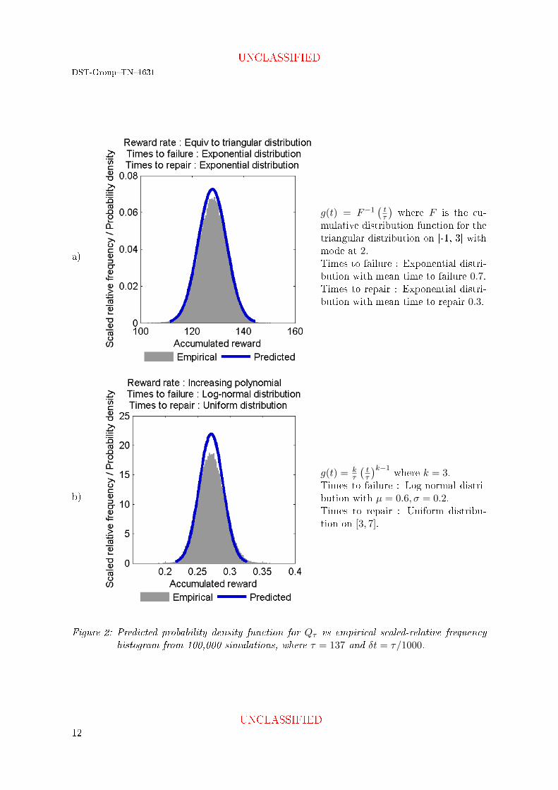
Figures 2 shows examples from experiments. In each case, the predicted distribution appearsto be a good approximation to the empirical distribution.

The author conjectures that the condition E(B3k), E(W 3

k ) < ∞ could be weakened to E(B2k),

E(W 2k ) <∞. This would match the assumption made by Takács [1959]. The condition E(B3

k),E(W 3

k ) < ∞ is used only to enforce α-mixing at the rate required by Peligrad's central limittheorem. Her theorem also holds under φ-mixing, and Glynn [1982, Theorem 6.3] states asu�cient condition for a regenerative process to be φ-mixing, but the present author wasunable to prove that E(B2

k), E(W 2k ) <∞ would satisfy Glynn's condition.

UNCLASSIFIED

11

DST-Group�TN�1631

UNCLASSIFIED

a)

g(t) = F−1(tτ

)where F is the cu-

mulative distribution function for thetriangular distribution on [-1, 3] withmode at 2.Times to failure : Exponential distri-bution with mean time to failure 0.7.Times to repair : Exponential distri-bution with mean time to repair 0.3.

b)

g(t) = kτ

(tτ

)k−1where k = 3.

Times to failure : Log-normal distri-bution with µ = 0.6, σ = 0.2.Times to repair : Uniform distribu-tion on [3, 7].

Figure 2: Predicted probability density function for Qτ vs empirical scaled-relative frequencyhistogram from 100,000 simulations, where τ = 137 and δt = τ/1000.

12UNCLASSIFIED

UNCLASSIFIED

DST-Group�TN�1631

5. Acknowledgements

The author thanks Maria Athanassenas, Jez Gray, Josef Zuk, and the anonymous referees fortheir constructive feedback.

6. References

Billingsley, P. (2008) Probability and measure, John Wiley & Sons, New York.

Durrett, R. (2005) Probability : Theory and Examples, 3rd edition edn, Thomson Brooks/Cole,Belmont, CA.

Glynn, P. W. (1982) Some New Results in Regenerative Process Theory, Technical Report 60,Department of Operations Research, Stanford University. URL � http://oai.dtic.mil/oai/oai?verb=getRecord&metadataPrefix=html&identifier=ADA119153.

Hew, P. C. (2017) Asymptotic distribution of rewards accumulated by alternating renewalprocesses, Statistics & Probability Letters 129, 355 � 359. URL � http://www.sciencedirect.com/science/article/pii/S0167715217302316.

Hoe�ding, W. & Robbins, H. (1948) The central limit theorem for dependent random variables,Duke Math. J. 15(3), 773�780. URL � http://dx.doi.org/10.1215/S0012-7094-48-01568-3.

Hoe�ding, W. & Robbins, H. (1985) The Central Limit Theorem for Dependent RandomVariables, Springer New York, New York, NY, pp. 349�356. URL � http://dx.doi.org/10.1007/978-1-4612-5110-1_30.

Ibragimov, I. A. (1975) A note on the central limit theorems for dependent random variables,Theory of Probability & Its Applications 20(1), 135�141.

Peligrad, M. & Utev, S. (1997) Central limit theorem for linear processes, The Annals ofProbability 25(1), 443�456. URL � http://dx.doi.org/10.1214/aop/1024404295.

Takács, L. (1959) On a sojourn time problem in the theory of stochastic processes, Trans.Amer. Math. Soc. 93(3), 531�540.

Trivedi, K. S. (2002) Probability and Statistics with Reliability, Queuing, and Computer ScienceApplications, second edn, John Wiley & Sons, New York.

UNCLASSIFIED

13

DST-Group�TN�1631

UNCLASSIFIED

This page is intentionally blank

14UNCLASSIFIED

UNCLASSIFIED

DST-Group�TN�1631

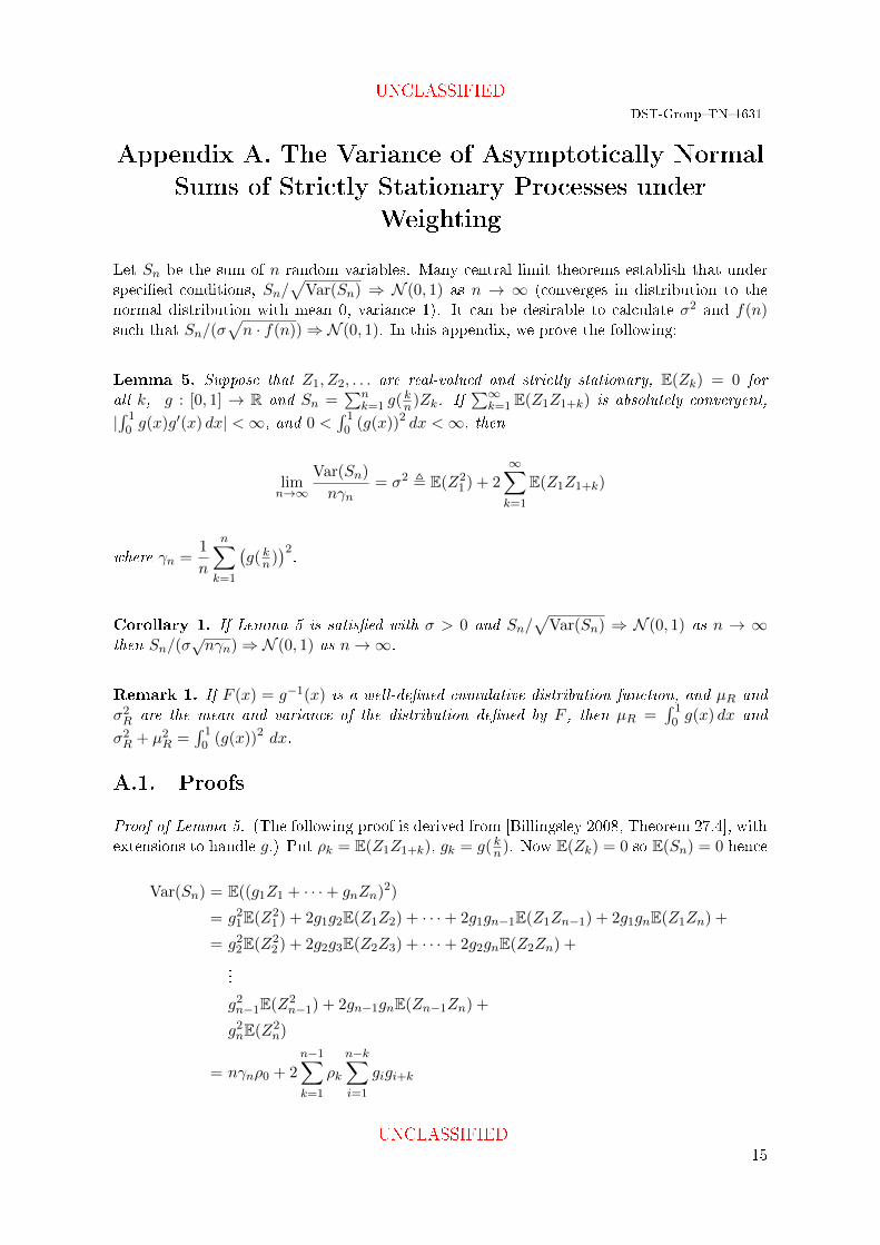
Appendix A. The Variance of Asymptotically Normal

Sums of Strictly Stationary Processes under

Weighting

Let Sn be the sum of n random variables. Many central limit theorems establish that underspeci�ed conditions, Sn/

√Var(Sn) ⇒ N (0, 1) as n → ∞ (converges in distribution to the

normal distribution with mean 0, variance 1). It can be desirable to calculate σ2 and f(n)such that Sn/(σ

√n · f(n))⇒ N (0, 1). In this appendix, we prove the following:

Lemma 5. Suppose that Z1, Z2, . . . are real-valued and strictly stationary, E(Zk) = 0 forall k, g : [0, 1] → R and Sn =

∑nk=1 g( kn)Zk. If

∑∞k=1 E(Z1Z1+k) is absolutely convergent,

|∫ 10 g(x)g′(x) dx| <∞, and 0 <

∫ 10 (g(x))2 dx <∞, then

limn→∞

Var(Sn)

nγn= σ2 , E(Z2

1 ) + 2

∞∑k=1

E(Z1Z1+k)

where γn =1

n

n∑k=1

(g( kn)

)2.

Corollary 1. If Lemma 5 is satis�ed with σ > 0 and Sn/√

Var(Sn) ⇒ N (0, 1) as n → ∞then Sn/(σ

√nγn)⇒ N (0, 1) as n→∞.

Remark 1. If F (x) = g−1(x) is a well-de�ned cumulative distribution function, and µR andσ2R are the mean and variance of the distribution de�ned by F , then µR =

∫ 10 g(x) dx and

σ2R + µ2R =∫ 10 (g(x))2 dx.

A.1. Proofs

Proof of Lemma 5. (The following proof is derived from [Billingsley 2008, Theorem 27.4], withextensions to handle g.) Put ρk = E(Z1Z1+k), gk = g( kn). Now E(Zk) = 0 so E(Sn) = 0 hence

Var(Sn) = E((g1Z1 + · · ·+ gnZn)2)

= g21E(Z21 ) + 2g1g2E(Z1Z2) + · · ·+ 2g1gn−1E(Z1Zn−1) + 2g1gnE(Z1Zn) +

= g22E(Z22 ) + 2g2g3E(Z2Z3) + · · ·+ 2g2gnE(Z2Zn) +

...

g2n−1E(Z2n−1) + 2gn−1gnE(Zn−1Zn) +

g2nE(Z2n)

= nγnρ0 + 2

n−1∑k=1

ρk

n−k∑i=1

gigi+k

UNCLASSIFIED

15

DST-Group�TN�1631

UNCLASSIFIED

as Z1, Z2, . . . is strictly stationary. Then

Var(Sn)

nγn= ρ0 + 2

n−1∑k=1

ρk1

nγn

n−k∑i=1

gigi+k

∣∣∣∣Var(Sn)

nγn− σ2

∣∣∣∣ = 2

∣∣∣∣∣∞∑k=n

ρk +

n−1∑k=1

(1− 1

nγn

n−k∑i=1

gigi+k

)ρk

∣∣∣∣∣= 2

∣∣∣∣∣∞∑k=n

ρk +n−1∑k=1

∑ni=1 g

2i −

∑n−ki=1 gigi+k

nγnρk

∣∣∣∣∣= 2

∣∣∣∣∣∞∑k=n

ρk +n−1∑k=1

∑ni=n−k+1 g

2i −

∑n−ki=1 (gigi+k − g2i )

nγnρk

∣∣∣∣∣= 2

∣∣∣∣∣∞∑k=n

ρk +

n−1∑k=1

αk + βkγn

k

nρk

∣∣∣∣∣where αk = − 1

n

∑n−ki=1 gi

gi+k−gik/n , βk = 1

k

∑ni=n−k+1 g

2i . Construct α(s) =

∫ s0 g(x)g′(x) dx and

β(s) =∫ 1s (g(x))2 dx, then α( kn) ≈ αk and β( kn) ≈ βk for any k < n. So if α∗ = sups∈[0,1]|α(s)|

and β∗ = sups∈[0,1]|β(s)| then∣∣∣∣Var(Sn)

nγn− σ2

∣∣∣∣ ≤ 2∞∑k=n

|ρk|+α∗ + β∗ + ε

nγn

n−1∑k=1

k|ρk|

for some small error term ε where ε→ 0 as n→∞. Moreover

n−1∑k=1

k|ρk| =

|ρ1| + |ρ2| + |ρ3| + · · ·+ |ρn−1| +|ρ2| + |ρ3| + · · ·+ |ρn−1| +

|ρ3| + · · ·+ |ρn−1| +...+ |ρn−1|

=n−1∑i=1

n−1∑k=i

|ρk|

≤n−1∑i=1

∞∑k=i

|ρk|

so ∣∣∣∣Var(Sn)

nγn− σ2

∣∣∣∣ ≤ 2

∞∑k=n

|ρk|+α∗ + β∗ + ε

nγn

n−1∑i=1

∞∑k=i

|ρk|

To complete the proof, we show that right-hand side converges to zero as n → ∞. In threesteps:

1.∑∞

k=1 ρk is absolutely convergent, so∑∞

k=n|ρk| → 0 as n→∞.

2. We have α∗, β∗ < ∞, 0 < limn→∞ γn < ∞ by the assumptions about g. Speci�cally: ifa function is integrable on [0, 1] then for any s it is integrable on the subintervals [0, s]and [s, 1]. Thus α(s) and β(s) are continuous on [0, 1], hence they are bounded on [0, 1].

16UNCLASSIFIED

UNCLASSIFIED

DST-Group�TN�1631

3. Put ζi =∑∞

k=i|ρk| and ωn−1 = 1n−1

∑n−1i=1 ζi. Now {ζi}i is decreasing so ωn → 0 as

n→∞. Hence1

n

n−1∑i=1

∞∑k=i

|ρk| =1

n

n−1∑i=1

ζi =n− 1

nωn−1 → 0

as n→∞.

Proof of Corollary 1. We have

Snσ√nγn

=Sn√

Var(Sn)·√

Var(Sn)

σ√nγn

So if Sn/√

Var(Sn)⇒ N (0, 1) and Lemma 5 is satis�ed with σ > 0, then the right hand sideconverges in distribution to N (0, 1) by Slutsky's theorem.

Proof of Remark 1.

1. µR =∫ g(1)g(0) x dF (x) by de�nition. Now

∫x dF (x) = xF (x)−

∫F (x) dx and∫

F (x) dx =

∫g−1(x) dx

=

∫tg′(t) dt via x = g(t)

=

[tg−1(t)−

∫g−1(t) dt

]= xF (x)−

∫g(x) dx

which yields

xF (x)−∫F (x) dx =

∫g(x) dx

Hence µR =∫ 10 g(x) dx.

2. σ2R + µ2R =∫ g(1)g(0) x

2 dF (x) by de�nition. Now∫x2 dF (x) = x2F (x)− 2

∫xF (x) dx and∫

xF (x)dx =

∫xg−1(x) dx

=

∫g(t)tg′(t) dt via x = g(t)

=

[g(t)tg(t)−

∫g(t)

(g(t) + tg′(t)

)dt

]=

[(g(t))2 t−

∫(g(t))2 dt−

∫g(t)tg′(t) dt

]

UNCLASSIFIED

17

DST-Group�TN�1631

UNCLASSIFIED

so

2

∫g(t)tg′(t) dt =

[(g(t))2 t−

∫(g(t))2 dt

]2

∫xF (x)dx = x2g−1(x)−

∫(g(x))2 dx

= x2F (x)−∫

(g(x))2 dx

which yields

x2F (x)− 2

∫xF (x) dx =

∫(g(x))2 dx

Hence σ2R + µ2R =∫ 10 (g(x))2 dx.

A.2. Remarks

If g(x) = 1 for all x then Lemma 5 reduces to the result obtained by Billingsley [2008,Theorem 27.4] and Durrett [2004, Theorem 7.8]. Billingsley and Durrett made additionalassumptions that lead to σ2 being well-de�ned and correct and asymptotic normality of Sn.The present author has extracted the assumptions and logic for σ2 so that it stands on itsown, in a form that can be used with other central limit theorems, and extended Billingsley'sproof to handle g.

If in addition to being identically distributed, the variables Z1, Z2, . . . are independent, thenσ2 = E(Z2

1 ) as per the classical Lindeberg�Lévy central limit theorem. If they arem-dependentthen σ2 = E(Z2

1 ) + 2∑m

k=1 E(Z1Z1+k), matching the calculations in the central limit theoremfor m-dependent sequences by Hoe�ding & Robbins [Theorem 2, 1948], [1985]. The authorconjectures that the calculations of variance made by Hoe�ding & Robbins and Ibraginov[1975, Theorem 2.2] could be extracted in the same way as was done here.

18UNCLASSIFIED

UNCLASSIFIED

DEFENCE SCIENCE AND TECHNOLOGY GROUP

DOCUMENT CONTROL DATA

1. DLM/CAVEAT (OF DOCUMENT)

2. TITLE

Asymptotic Distribution of Rewards Accumulated by AlternatingRenewal Processes

3. SECURITY CLASSIFICATION (FOR UNCLASSIFIED LIMITED

RELEASE USE (L) NEXT TO DOCUMENT CLASSIFICATION)

Document (U)Title (U)Abstract (U)

4. AUTHORS

Patrick Chisan Hew

5. CORPORATE AUTHOR

Defence Science and Technology Group506 Lorimer St,Fishermans Bend, Victoria 3207, Australia

6a. DST GROUP NUMBER

DST-Group�TN�1631

6b. AR NUMBER

016-866

6c. TYPE OF REPORT

Technical Note

7. DOCUMENT DATE

October 2017

8. OBJECTIVE ID

qAV22220

9. TASK NUMBER

NAV 17/525

10. TASK SPONSOR

Director General SEA1000

11. MSTC 12. STC

13. DOWNGRADING/DELIMITING INSTRUCTIONS

http://dspace.dsto.defence.gov.au/dspace/

14. RELEASE AUTHORITY

Chief, Joint and Operations Analysis Division

15. SECONDARY RELEASE STATEMENT OF THIS DOCUMENT

Approved for Public Release

OVERSEASENQUIRIESOUTSIDESTATEDLIMITATIONSSHOULDBEREFERREDTHROUGHDOCUMENTEXCHANGE,POBOX1500,EDINBURGH,SA5111

16. DELIBERATE ANNOUNCEMENT

No Limitations

17. CITATION IN OTHER DOCUMENTS

No Limitations

18. RESEARCH LIBRARY THESAURUS

probability theory: asymptotically normal, stochastic processes: alternating renewal process, reward

19. ABSTRACT

This technical note considers processes that alternate randomly between `working' and `broken' over an interval of time. Suppose thatthe process is rewarded whenever it is `working', at a rate that can vary during the time interval but is known completely. We prove thatif the time interval is long then the accumulated reward is approximately normally distributed and the approximation becomes perfectas the interval becomes in�nitely long. Moreover we calculate the means and variances of those normal distributions. Formally, consideran alternating renewal process on the states `working' vs `broken'. Suppose that during any interval [0, τ ], the process is rewarded atrate g(t/τ) if it is working at time t. Let Qτ be the reward that is accumulated during [0, τ ]. We calculate µQτ and σ2

Qτsuch that

(Qτ − µQτ )/σQτ converges in distribution to a standard normal distribution as τ →∞.

UNCLASSIFIED