1

Asymmetric growth effect of capital flows: Evidence and quantitative theory

Yoke-Kee Enga Chin-Yoong Wonga,b,

aDepartment of Economics, Universiti Tunku Abdul Rahman, Malaysia bStockholm China Economic Research Institute, Stockholm School of Economics

Abstract

Empirical evidence of the causal relationship between capital flows and economic growth

over the decades is largely indecisive. While the promised benefits to countries that open for capital

inflows have not been realized, sudden and massive capital outflows often visibly wreak havoc on the

economy. By using the recently developed asymmetric Granger causality test, we find overwhelming

evidence across nine selected Asian countries in support of asymmetric effect of capital flow on

economic growth in the sense that cumulative capital inflows are growth irrelevant, whereas cumulative

capital outflows are growth destructive. Based on a small open-economy model expanded with

heterogeneous investment goods and endogenous nonlinear credit constraint, we provide an economic

intuition for the asymmetry that survives different level of financial developments. In particular, arbitrage

condition between heterogeneous investment goods sets a boundary over which massive and

persistent capital inflows would leave no impact on long-run growth. Whereas endogenous nonlinear

credit constraint triggers debt deflation process, making large and persistent capital outflows growth

destructive.

Keywords: Capital flows; Economic growth; Asymmetric Granger causality test; Investment composition; Nonlinear credit constraint

Correspondence author. Faculty of Business and Finance, Universiti Tunku Abdul Rahman, Jalan Universiti, Bandar Barat,

31900 Kampar, Perak, Malaysia. Tel.: +6054688888 ext. 4337; fax: +6054667407. Email address: engyk@utar.edu.my (Eng

Y.-K.); wongcy@utar.edu.my (Wong C.-Y). This paper is revised when the second author is hosted by SCERI as Visiting

Research Fellow. He is grateful to SCERI for conducive research environment and Lars-Erik Thunholms Stiftelse for

Vetenskaplig Forskning for generous stipend. This research is part of a project financially funded by Fundamental Research

Grant Scheme (FRGS) from the Ministry of Education, Malaysia (FRGS/2/2013/SS07/UTAR/02/1).

2

1. Introduction

Prior to the onset of the Asian financial meltdown in 1997/98, East and Southeast Asian

emerging economies that liberalized capital accounts in the early 1990s were the darlings of

international investors. The fast and stable economic expansion during that time was often claimed to

be the outcome of capital account liberalization. As the crisis unfolded and capital flows suddenly

reversed from net inflow to outflow in 1997, one economy after another fell sharply into deep recession.

With the benefit of hindsight, we now learn that while it remains empirically dubious to attribute the

miraculous economic growth to massive capital inflows in the early 1990s, it is beyond controversy to

associate the Asian economic recession with the drastic capital outflows.

In fact, the evidence of asymmetric relationships between capital flows and economic growth

extends beyond Asia. From the one perspective, after decades of effort spent searching for answers to

the question of whether capital account liberalization spurs growth, the evidence in support of this

premise is weak. Although some have found a positive effect conditional on the existence of good

institutions, legitimate doubts are often cast on the robustness and context-sensitivity of such a

conditional effect (see, for instance, Jeanne et al., 2012; Kose et al., 2009a; Kose et al., 2009a; Gamra,

2009). Prasad et al. (2007) and Gourinchas and Jeanne (2006) have even found that the fastest

growing countries did so without much foreign capital.

On the other hand, a sudden stop in capital flows has been the recurring theme of financial

and economic crises. A massive capital flow reversal depreciates the exchange rate and plunges asset

prices, which, in turn, devalues the worth of collateral for borrowing, thus instigating an adverse

balance-sheet effect on domestic agents indebted in foreign currency. The resulting contraction in

aggregate demand amplifies the damaging deleveraging process (Jeanne et al., 2012). The common

thread that links currency crash and financial and economic crises is foreign currency debt (see, for

instance, Bordo et al., 2010; Bordo and Meissner, 2006). In other words, in the absence of foreign

currency debt, a slump in the currency driven by capital flows reversal is not likely to trigger the

3

balance-sheet effect and poses no immediate threat to the economy. This finding is evidenced by the

resilience of emerging economies to weather the storm of capital flow reversals during the recent global

financial crisis, despite the fact that disruption in cross-border capital flows seriously affected the

advanced economies (Tille, 2012).

Motivated by these observations, the first goal of this paper is to formally investigate whether

there is an asymmetric causal relationship between capital flow and economic growth. While our paper

naturally fits into the larger literature on the growth effect of capital inflow, we hope it is useful in this

enterprise by addressing different questions. We rethread the old song of “whether net capital flow

precedes growth” with a new chorus: Does net capital flow asymmetrically precede growth? Are net

capital inflows irrelevant to growth while net capital outflows being detrimental to growth? We address

this question in Section 2 by using the asymmetric Granger causality testing procedures recently

developed by Hatemi-J’s (2012). We for the first time find overwhelming evidence, as elaborated in

Section 3, across nine selected Asian countries in support of such asymmetry, in that cumulative capital

inflows are found to be growth irrelevant whereas cumulative capital outflows are found to be growth

destructive. The results also decisively reject the possibility of reverse causality from growth to capital

flows.

Having quantified the asymmetry, our second goal is to find out why: What causes the

asymmetry? Drawn on a quantitative model developed in Section 4, the underlying mechanisms are

heterogeneous investment goods, inspired by Aghion et al. (2010), and endogenous nonlinear credit

constraint in the spirit of vast literature on sudden stops and Fisherian deflation (Calvo et al., 2006;

Bianchi, 2011; Mendoza, 2010; Korinek and Mendoza, 2014). Of different types of investments, we

assume that only long-term investment contributes to long-run growth. Arbitrage condition between

short-term and long-term investments, effectuated by the law of diminishing marginal return, embeds an

upper bound, over which even persistently massive portfolio capital inflows would not incentivize long-

term investments and hence would have no effects on long-run growth.

4

By assuming that long-term investment requires financing, which can be sourced either from

the regulated domestic financial intermediaries or the competitive foreign creditors, optimal long-term

investment decision is influenced by the conventional opportunity cost and credit constraint as well.

Because the latter is endogenous to the entrepreneur’s creditworthiness in nonlinear fashion, a binding

credit constraint due to large and persistent portfolio capital outflows or a sudden stop (massive capital

flows reversal) can trigger debt deflation process. Deteriorating creditworthiness reinforces cutback in

the cheaper foreign financing, making only the more expensive domestic credits available for long-term

investment.

Nevertheless, debt-deflation process is not explosive, as the resultant increasing marginal

return on long-term capital stock would make long-term investment profitable even when it is financed

by the more expensive domestic credits. Gradually restored long-term investment revives long-run

growth over time. In Section 5, we further show that our mechanism of asymmetry survives different

levels of financial development.

2. Does capital flow precede growth? An asymmetric Granger causality approach

Consider a p-th order bivariate system of invertible stationary processes for output 𝑌𝑡 and net

capital flow 𝒞ℱ𝑡, as in the following autoregressive representation:

[𝑌𝑡𝒞ℱ𝑡

] = 𝕒0 + ∑ [𝛼11,𝑖 𝛼12,𝑖𝛼21,𝑖 𝛼22,𝑖

] [𝑌𝑡−𝑖𝒞ℱ𝑡−𝑖

]𝑝𝑖=1 + [

휀𝑌,𝑡휀𝒞ℱ,𝑡

] (1)

where 𝕒0 is a vector of deterministic terms, 𝛼𝑗𝑘,𝑖 for 𝑗, 𝑘 = 1,2 are finite polynomials, 휀𝑌,𝑡(=

∑ 휀𝑌,𝑡+𝑖𝑝𝑖=0 ) and 휀𝒞ℱ,𝑡(= ∑ 휀𝒞ℱ,𝑡+𝑖

𝑝𝑖=0 ) are taken to be two uncorrelated white-noise series where

𝐸[휀𝒞ℱ,𝑡휀𝒞ℱ,𝑠] = 𝐸[휀𝑌,𝑡휀𝑌,𝑠] = 0. Then, for 𝛼12,𝑖 = 0, where 𝑖 = 1,2, … , 𝑝, we contend that capital

flow is not Granger-causal for output growth as none of its lags appears in the 𝑌𝑡 equation. In other

5

words, capital flow is Granger-causal for output growth if at least one of the 𝛼12,𝑖 is not zero. This is the

standard Granger causality test principle.

That said, the shortcomings of the standard Granger causality test are obvious. For example,

the test has nothing to say about whether it is the capital inflow or outflow that Granger causes growth,

it sheds no light on whether capital flow (either in or out) Granger causes positive or negative economic

growth, and hence, it does not allow an asymmetric Granger causal relationship. To address this

shortcoming, we make use of the asymmetric Granger causality test recently developed by Hatemi-J

(2012). Hatemi-J (2012) extends the idea originated in Granger and Yoon (2002) of decomposing the

stochastic disturbance terms into positive and negative shocks. With respect to our context, it means

that we can now explicitly decompose the causal impact of positive changes in capital flows (which

indicate net inflows) from the negative changes (which indicate net outflows).

The intuition is simple. Assume that capital flow and economic growth follow a random walk in

such a way that

𝒞ℱ𝑡 = 𝒞ℱ𝑡−1 + 휀𝒞ℱ,𝑡 = 𝒞ℱ10 + ∑ 휀𝒞ℱ𝑖𝑡𝑖=1 (2)

𝑌𝑡 = 𝑌𝑡−1 + 휀Y,𝑡 = 𝑌20 +∑ 휀𝑌𝑖𝑡𝑖=1 (3)

where 𝑡 = 1,2, … , 𝑇 denotes discrete-time periods, the constants 𝒞ℱ10 and 𝑌20 indicate the initial

values for capital flow and economic growth, respectively, and 휀𝒞ℱ𝑖 and 휀𝑌𝑖 are white-noise

disturbance terms. We decompose the disturbance terms into positive and negative shocks

휀𝒞ℱ𝑖 = 휀𝒞ℱ𝑖+ + 휀𝒞ℱ𝑖

− (4)

휀𝑌𝑖 = 휀𝑌𝑖+ + 휀𝑌𝑖

− (5)

where 휀𝒞ℱ𝑖+ = max(휀𝒞ℱ𝑖, 0) , 휀𝒞ℱ𝑖

− = min(휀𝒞ℱ𝑖, 0) , 휀𝑌𝑖+ = max(휀𝒴𝑖, 0) , and 휀𝑌𝑖

− = min(휀𝒴𝑖 , 0) .

Eqs. (2) and (3) can then be rewritten as

𝒞ℱ𝑡 = 𝒞ℱ𝑡−1 + 휀𝒞ℱ,𝑡 = 𝒞ℱ10 + ∑ 휀𝒞ℱ𝑖+𝑡

𝑖=1 + ∑ 휀𝒞ℱ𝑖−𝑡

𝑖=1 (6)

𝑌𝑡 = 𝑌𝑡−1 + 휀𝑌,𝑡 = 𝑌20 + ∑ 휀𝑌𝑖+𝑡

𝑖=1 + ∑ 휀𝑌𝑖−𝑡

𝑖=1 (7)

6

The cumulative positive and negative shocks, respectively, constitute capital inflows (economic growth)

and capital outflows (economic downturn) in such a way that

𝒞ℱ𝑡+ = ∑ 휀𝒞ℱ𝑖

+𝑡𝑖=1 (8)

𝒞ℱ𝑡− = ∑ 휀𝒞ℱ𝑖

−𝑡𝑖=1 (9)

𝑌𝑡+ = ∑ 휀𝑌𝑖

+𝑡𝑖=1 (10)

𝑌𝑡− = ∑ 휀𝑌𝑖

−𝑡𝑖=1 (11)

This implies that each shock has a long-lasting effect on the underlying variable. With these variables,

we can test for asymmetric causality using the standard vector autoregressive model of order p, VAR(p).

Suppose we are interested to test the causal relationship between capital inflows and economic growth.

Eq. (1) now reads

𝕪𝑡+ = 𝕒0 + A1𝕪𝑡−1

+ +⋯+ A𝑝𝕪𝑡−𝑝+ + 𝕦𝑡

+ (12)

where 𝕪𝑡+ = [𝑌𝑡

+ 𝒞ℱ𝑡+]′ and 𝕦𝑡

+ is a 2 x 1 vector of the cumulative sum of positive error terms. The

null hypothesis that capital inflow is not Granger-causal for economic growth can be tested depending

on whether row 𝑗, column 𝑘 elements in A𝑟, where 𝑗 = 1, 𝑘 = 2, equal zero for 𝑟 = 1,… , 𝑝. By the

same token, we can test whether capital outflow Granger-cause economic downturn by examining

𝕪𝑡− = 𝕒0 + A1𝕪𝑡−1

− +⋯+ A𝑝𝕪𝑡−𝑝− + 𝕦𝑡

− (13)

In this paper, we test four combinations for each direction of causality.

The optimal lag order (p) is selected based on the information criteria suggested by Hatemi-J

(2003), which proves to be robust for the ARCH effect and performs well when the VAR model is used.

HJC = ln(|Ω̂𝑗|) + 𝑗 (𝑛2 ln𝑇+2𝑛2 ln(ln𝑇)

2𝑇) (14)

where 𝑗 = 0, … , 𝑝, |Ω̂𝑗| is the determinant of the estimated variance-covariance matrix of the error

terms in the VAR (𝑗) model, 𝑛 is the number of equations the VAR model has, and 𝑇 is the number of

observations. As suggested in Hatemi-J (2012) and following Toda and Yamamoto (1995), additional

unrestricted lag is added to the VAR model to accommodate the effect of one unit root. Given the short

time span of data, we apply the bootstrapping simulation technique as detailed in Hatemi-J (2008). This

7

technique helps to achieve better size and power properties compared to the test that is based on

asymptotical distribution. It also makes causality test foolproof to outliers in capital flows due to sudden

stop episodes during 1997/98 and 2008/09. The bootstrapped critical values are generated at three

different levels of significance based on ten thousand repetitions of the simulation. Interested readers

can refer to Hatemi-J (2012) for technical details.

3. Empirical findings

3.1 The data

We collect annual time-series data that spans over 32 years, 1980 to 2011, for nominal gross

domestic products (GDP), current account, and capital account for nine Asian countries, including

China, India, Indonesia, Japan, Republic of Korea, Malaysia, the Philippines, Singapore and Thailand.

The data are sourced from International Financial Statistics and Balance of Payments Statistics issued

by the International Monetary Fund. Divided by population, the resultant per capita nominal GDP is then

adjusted for purchasing power parity (PPP) in terms of the U.S. dollar and takes the form of a natural

logarithm. In short, we call PPP-adjusted per capita GDP the per capita real GDP.

Current account and capital account as a share of GDP are used as two different proxies for

net capital flows. While the former encompasses both official and private capital flows, the latter reflects

pure private capital flows. Last, we turn the value of the current account balance to the opposite sign so

that current account surplus (deficit) can be easily interpreted as capital outflow (inflow). The time plots

of the current account as a share of GDP (-CA/GDP) and the capital account as a share of GDP

(KA/GDP), along with real GDP growth rate, are as shown in Figure 1, and the time plots of the real

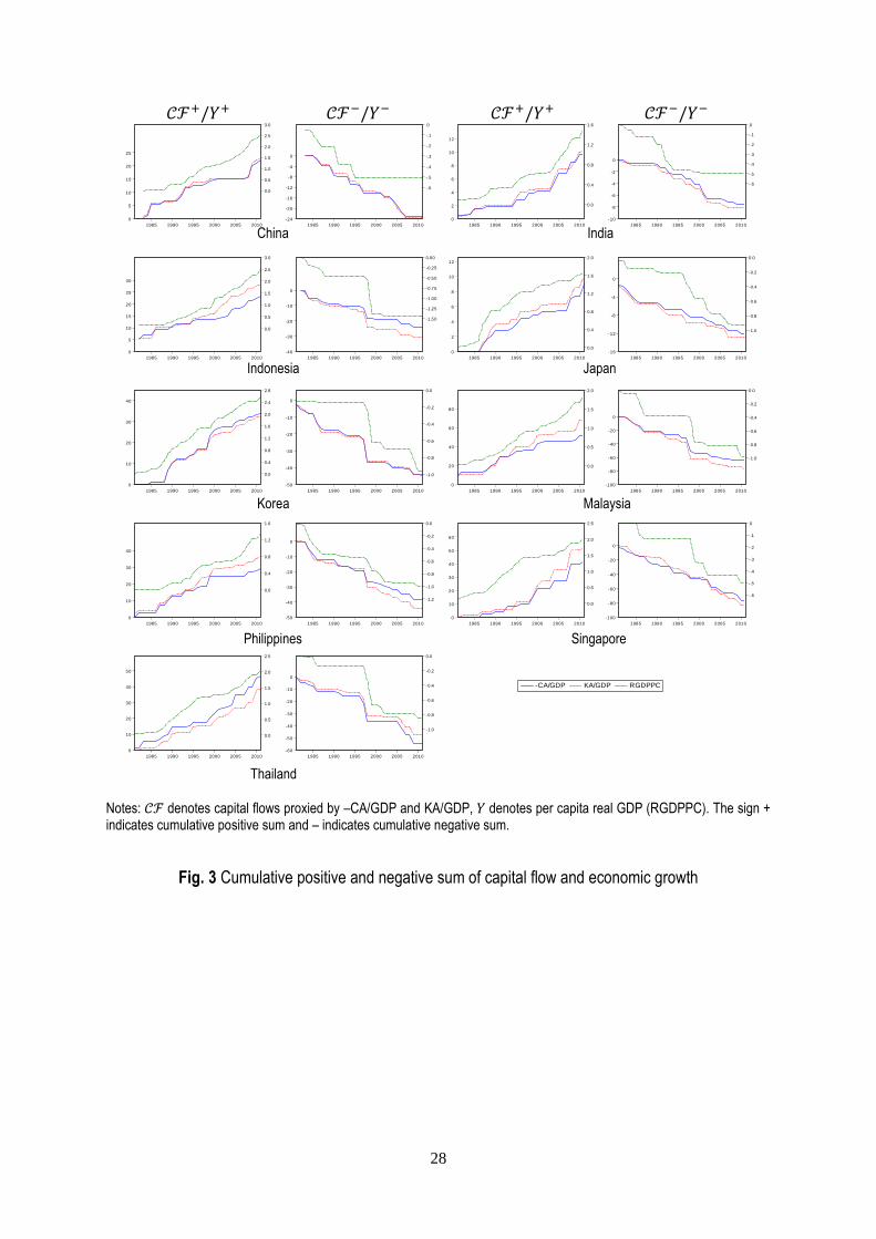
GDP per capita in logarithm value are shown in Figure 2. Figure 3 describes the cumulative positive

and negative sums of per capita real GDP and capital flows represented by -CA/GDP and KA/GDP,

respectively. Causality that runs from capital flow (in and out) to the economy (growth and downturn),

and vice versa, for each country are formally tested. As each direction of causality involves four

8

hypotheses with two different proxies for capital flow, there are a total of 144 causality tests to be

conducted.

[INSERT FIGURES 1, 2, and 3 HERE]

Before proceeding to formal testing, it is worthwhile to eyeball the asymmetric relationship

between capital flows and real economic growth over time in Figure 1. At first glance, there are many

instances in which capital outflows are associated with falling economic growth, particularly during the

Asian currency and financial crises. However, a case such as Thailand, where capital inflows are

clearly associated with rising economic growth, is the exception rather than the norm. More puzzling is

the observation that capital outflows occur along with rising economic growth. China’s economic

expansion after year 2000, for instance, has witnessed continuous capital outflows as did Malaysia, the

Philippines, and Singapore after the year 2002.

3.2 Pre-testing

Preceding asymmetric causality testing, we need to determine whether unit roots are present in

the time series. To do so, we use the Dickey-Fuller generalized least squares (DF-GLS) test. This test

dominates the ordinary DF test in terms of small sample size and power (Elliott et al., 1996). Though

not shown (but available upon request), the series are all difference-stationary. However, the causality

test between integrated series remains to be implemented within the VAR-in-level framework without

pre-testing for co-integration. Gospodinov et al. (2013) have recently shown that VAR-in-level

specification is robust to the potential uncertainty about exact integration and co-integration properties

of the data. This is supported by the seminal Toda and Yamamoto (1995) that co-integration does not

matter with respect to causality testing when additional lags of each variable based on the maximum

order of integration are added to the model.

3.3 Results

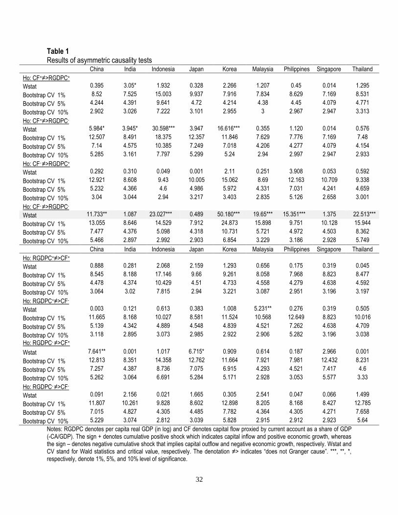
Table 1 reports the results of the asymmetric causality test when –CA/GDP is used as a proxy

for capital flows. The findings are overwhelmingly in favor of the asymmetric relationship between

9

capital flow and economic growth in that cumulative capital inflows (𝒞ℱ𝑡+) do not Granger-cause

economic growth (𝒴𝑡+) , whereas cumulative capital outflows (𝒞ℱ𝑡

−) Granger-cause economic

downturn (𝒴𝑡−) with strong statistical significance. Meanwhile, with very few exceptions, other null

hypotheses for different combinations of cumulative capital flows and economic growth cannot be

rejected at any widely accepted level of significance. Table 1 also convincingly demonstrates that

economic growth performance does not Granger-cause capital flow. All these findings are robust to

different proxies for capital flows. Table 2 shows the results of the asymmetric causality test when

KA/GDP, which considers only private capital flows, is used in the tests. The finding that capital outflow

is growth-crashing remains true and that capital inflow is growth-irrelevant also holds.

[INSERT TABLES 1 and 2 HERE]

4. Modeling the asymmetry

What causes the asymmetry? In this section, we lay out a small open-economy model to

account for the asymmetric effect of capital flows on economic growth. The key property is the

combination of heterogeneous investment goods and endogenous nonlinear credit constraint. The latter

is drawn on a large literature on sudden stop (see Korinek and Mendoza, 2014 for an overview of a

class of models that explain stylized facts of sudden stop) However, what differentiates ours from

sudden stop literature is the mechanism of growth-destructive sudden stop.

Instead of resorting to asset price amplification to initiate debt-deflation process, we bring in

Aghion et al.’s (2010) insight on short-term versus long-term investments. By short term we mean the

corresponding capital stock has lower gross marginal return and contributes only to short-term growth.

In contrast, long-term capital stock has higher gross marginal return but needs financing, and

contributes to long-term growth. We shall see later how such a simple device not only enables us to

trigger a debt-deflation process, but also to account for the asymmetric effects of capital flows on long-

run economic growth.

4.1 Long-run growth equation

10

Following Aghion and Howitt (2008, p.331), we define long-term economic growth as first

difference in productivity trend due to accumulation of long-term capital stock

Δ𝑇𝑡 ≡ ln𝑇𝑡 − ln𝑇𝑡−1 = ℱ (𝑍𝑡

𝑍𝑡−1− 1) (15)

where 𝑇𝑡 denotes productivity trend, 𝑍𝑡 is long-term capital stock, and ℱ is the fraction of

entrepreneurs who can access to credit market. A financial market is well developed and unrestricted

when credit is accessible for all entrepreneurs, facilitating entrepreneurial undertaking in long-term

investment that leads to long-run growth. For that we have ℱ = 1. In other words, an underdeveloped

financial market, in which ℱ approximates zero, holds back incentive for long-term investment, limiting

long-run growth.

We can also interpret ℱ in terms of financial market’s ability to monitor borrowers’ behavior ex

post borrowing. Better monitoring, which indicates more advanced financial system, minimizes moral

hazard incidence, ensuring a higher proportion of credit-financed long-term investment acquisition that

leads to greater long-run growth. The parameter ℱ is thus one of the two indicators for domestic

financial development in this paper.

4.2 Household as entrepreneur and debtor with endogenous credit constraint

Our model economy is populated by a unit mass of households. In each period, they work for

wage income 𝑊𝑡, they consume 𝐶𝑡, they accumulate wealth in the form of domestic 𝐵𝑡 and foreign

bonds 𝐵𝑡∗, and they invest in short-term 𝐼𝐾,𝑡 and long-term investment goods 𝐼𝑍,𝑡. Each investment, be

it physical or financial, contributes to the stock accumulation that earns them a return. Flow budget

constraint and stock constraints for a household take the form

𝐵𝑡−(1+𝑟𝑡−1)𝐵𝑡−1

𝑃𝑡+ 𝐶𝑡 + 𝐼𝐾,𝑡 + 𝐼𝑍,𝑡 +𝕂ℎ𝑓,𝑡 +Φ𝐾,𝑡𝐾𝑡−1 +Φ𝑍,𝑡𝑍𝑡−1 +Φ𝕂,𝑡𝑆𝑡

𝐵𝑡−1∗

𝑃𝑡+

(1 + 𝑟𝐿,𝑡)𝐿𝑡−1

𝑃𝑡+ (1 + 𝑟𝐿,𝑡

∗ ) (𝑆𝑡

𝑃𝑡) 𝐿𝑡−1

∗ = 𝑟𝐾,𝑡𝐾𝑡−1 + 𝑟𝑍,𝑡𝑍𝑡−1 +𝑊𝑡𝑁𝑡 (16)

11

𝐾𝑡 = (1 − 𝛿𝐾)𝐾𝑡−1 + exp(휁𝐾,𝑡) 𝐼𝐾,𝑡 (17)

𝑍𝑡 = (1 − 𝛿𝑧)𝑍𝑡−1 + exp(휁𝑍,𝑡) 𝐼𝑍,𝑡 (18)

𝑆𝑡𝐵𝑡∗

𝑃𝑡= (1 + 𝑟𝑡−1

∗ )𝑆𝑡𝐵𝑡−1

∗

𝑃𝑡+ exp(휁𝕂,𝑡)𝕂ℎ𝑓,𝑡 (19)

where 𝑆𝑡 refers to domestic value of a foreign currency, and 𝑒𝑡(= 𝑆𝑡𝑃𝑡∗ 𝑃𝑡⁄ ) is real exchange rate.

Eqs. (16) and (17) are the law of motion of short-term and long-term capital stock, respectively, with 𝛿𝑖

indicates deprecation rate. 휁𝐾,𝑡 and 휁𝑍,𝑡 are first-order autoregressive investment-specific technology

shock hitting short-term and long-term investment. Eq. (19) simply puts forward a point that difference

between the end of current and last year’s stocks of foreign bonds constitutes a capital outflow from

home to foreign countries 𝕂ℎ𝑓,𝑡 , net of the reinvestment of interest earnings. 휁𝕂,𝑡 is first-order

autoregressive capital outflow shocks by domestic residents. Besides, every capital and portfolio

adjustment involves adjustment cost, which takes quadratic form. In particular, we model the

adjustment cost

Φ𝐾,𝑡 =1

2Φ𝐾 (

𝐼𝐾,𝑡

𝐾𝑡−1− 𝛿)

2

; Φ𝑍,𝑡 =1

2Φ𝑍 (

𝐼𝑍,𝑡

𝑍𝑡−1− 𝛿)

2

; Φ𝕂,𝑡 =1

2Φ𝕂 (

𝑃𝑡𝕂ℎ𝑓,𝑡

𝑆𝑡𝐵𝑡−1∗ − 𝛿𝕂) (20)

where Φ𝑖 is a scale parameter.

Last but not least, note that there are two types of loans to be serviced by a household in every

period’s flow budget constraint (16). She has to service principal and interest for real domestic loans

𝐿𝑡−1 𝑃𝑡⁄ , and as well real foreign loans in domestic currency 𝑆𝑡𝐿𝑡−1∗ 𝑃𝑡⁄ . High price level reduces real

burden, while depreciated currency at date 𝑡 amplifies burden incurred at one period earlier. The

borrowing is made due to the financing requirement for long-term physical investment. She has to

secure loans one period earlier before an investment undertaking either from domestic source that

costs an interest rate of 𝑟𝐿,𝑡 or foreign source of funds at a rate of 𝑟𝐿,𝑡∗ . We assume that foreign

intermediaries are competitive with unregulated interest rate, and hence are able to offer a lending rate

12

that adjusts along its cost of funds, 𝑟𝐿,𝑡∗ = 𝑟𝑡

∗. On the other hand, domestic financial intermediaries

suffer from financial repression that takes the form of controlled interest rate. For the sake of simplicity,

we assume a constant (regulated) interest margin by 𝑐 to give 𝑟𝐿,𝑡 = 𝑟𝑡 + 𝑐 . This is the second

characteristic of imperfect domestic financial market, which accommodates for the fact that allowing for

foreign borrowing at cheaper cost relaxes borrowing constraint, leading to higher investment and higher

average growth (Ranciere et al., 2006).

Let 𝜌𝑡 be the fraction of long-term investment financed by the cheaper foreign loans, whereas

the remaining 1 − 𝜌𝑡 indicates the fraction financed by the more expensive domestic credits. Credit-in-

advanced constraints for long-term investment can be presented as

𝜌𝑡𝐼𝑍,𝑡 = 𝑆𝑡−1𝐿𝑡−1∗ 𝑃𝑡−1⁄ (21)

(1 − 𝜌𝑡)𝐼𝑍,𝑡 = 𝐿𝑡−1 𝑃𝑡−1⁄ (22)

Whether the entrepreneur can finance long-term investment entirely by foreign loans depends on her

creditworthiness. We let her creditworthiness depends on the value of profit that can be generated from

the investment, 𝜛Π𝑡, where 𝜛 is a scale parameter. Therefore the entrepreneur will undertake long-

term investment with cheaper foreign finance whenever profit generated is at least as large as total

foreign debt obligation in local currency, 𝜛Π𝑡 ≥ 𝑒𝑡(1 + 𝑟𝐿,𝑡∗ )𝐿𝑡

∗ . Thus, probability of obtaining foreign

loans, which can be comprehended as endogenous creditworthiness, is equal to

𝜌𝑡 = exp(−𝑒𝑡(1 + 𝑟𝐿,𝑡∗ )𝐿𝑡

∗ 𝜛Π𝑡⁄ ) (Endogenous creditworthiness) (23)

For strong profit performance such that 𝜛Π𝑡 > 𝑒𝑡(1 + 𝑟𝐿,𝑡∗ )𝐿𝑡

∗ , 𝜌𝑡 = exp(−0) ≈ 1. Otherwise, the

entrepreneur has to opt for domestic loans that are more expensive but less stringent on

creditworthiness requirement in securing loans, as 𝜌𝑡 < 1,.

13

Household optimally chooses the sequences of 𝐶𝑡, 𝑁𝑡, 𝐵𝑡, 𝕂ℎ𝑓,𝑡, 𝐵𝑡∗, 𝐼𝐾,𝑡, 𝐾𝑡, 𝐼𝑍,𝑡, 𝑍𝑡, 𝐿𝑡

∗ , 𝐿𝑡 to

maximize the following utility function

𝑢 = 𝔼𝑡 [∑𝛽𝑡 exp(휁𝐻,𝑡) (𝐶𝑡1−𝜎

1 − 𝜎−𝑁𝑡1+𝜒

1 + 𝜒)

∞

𝑡=0

]

subject to flow constraint (16), stock constraints (17) to (19), and credit-in-advance constrains (21) to

(22). 𝜎 is the risk aversion parameter, 𝜒 is wage elasticity of labor supply, and 𝛽 is subject discount

factor. 휁𝐻,𝑡 is first-order autoregressive preference shock. Consumption bundles 𝐶𝑡 consist of locally

produced 𝐶ℎ,𝑡 and imported consumer goods 𝐶𝑓ℎ,𝑡 in CES fashion at market price of 𝑃ℎ,𝑡 and 𝑆𝑡𝑃𝑓ℎ,𝑡∗ .

The latter indicates a complete exchange rate pass-through into import price as export goods are

invoiced at producer currency. We assume that price is set as a markup over real marginal cost,

𝑃ℎ,𝑡 = 𝜇Θ𝑡. Optimal demand for local and imported consumer goods takes the following form

𝐶ℎ,𝑡 = 𝛾(𝑃ℎ,𝑡 𝑃𝑡⁄ )−𝜑𝐶𝑡 (24)

𝐶𝑓ℎ,𝑡 = (1 − 𝛾)(𝑆𝑡𝑃𝑓ℎ,𝑡∗ 𝑃𝑡⁄ )

−𝜑𝐶𝑡 (25)

where 𝑃𝑡 is utility-based consumer price index

𝑃𝑡 = (𝛾𝑃ℎ,𝑡1−𝜑 + (1 − 𝛾)(𝑆𝑡𝑃𝑓ℎ,𝑡

∗ )1−𝜑

)1 (1−𝜑)⁄

(26)

By denoting 𝜆𝑡, Ω𝐾,𝑡, Ω𝑍,𝑡, Λ𝑡, 𝜚𝑡′ , 𝜚𝑡 , respectively, as Langragian multiplier for Eqs. (16) to

(19), and (21) and (22), the first-order conditions are

𝛽𝑡 exp(휁𝐻,𝑡) 𝐶𝑡−𝜎 = 𝜆𝑡 (27)

𝐶𝑡𝜎𝑁𝑡

𝜒 = 𝑊𝑡 (28)

𝜆𝑡+1(1 + 𝑟𝑡)𝑃𝑡 = 𝜆𝑡𝑃𝑡+1 (29)

14

𝕂ℎ𝑓,𝑡 = 𝑆𝑡𝐵𝑡−1∗

𝑃𝑡(1

Φ𝕂(𝑞𝕂,𝑡 exp(휁𝕂,𝑡) − 1) + 𝛿𝕂) (30)

𝑞𝕂,𝑡 = 𝔼𝑡 (𝑆𝑡+1

𝑆𝑡) (

1

1+𝑟𝑡) (𝑞𝕂,𝑡+1(1 + 𝑟𝑡

∗) + 𝑝𝑎𝑐𝑡+1) (31)

𝐼𝐾,𝑡 = 𝐾𝑡−1 (1

Φ𝐾(𝑞𝐾,𝑡 exp(휁𝐾,𝑡) − 1) + 𝛿𝐾) (32)

𝑞𝐾,𝑡 = 𝔼𝑡 (𝑃𝑡+1

𝑃𝑡) (

1

1+𝑟𝑡) (𝑞𝐾,𝑡+1(1 − 𝛿𝐾) + 𝑟𝐾,𝑡+1 + 𝑘𝑎𝑐𝑡+1) (33)

𝐼𝑍,𝑡 = 𝑍𝑡−1(1

Φ𝑍(𝑞𝑍,𝑡 exp(휁𝑍,𝑡) − 1⏟

𝑜𝑝𝑝𝑜𝑟𝑡𝑢𝑛𝑖𝑡𝑦 𝑐𝑜𝑠𝑡

−𝜌𝑡 (𝜚𝑡′

𝜆𝑡) − (1 − 𝜌𝑡) (

𝜚𝑡

𝜆𝑡)

⏟ 𝑙𝑖𝑞𝑢𝑖𝑑𝑖𝑡𝑦 𝑐𝑜𝑛𝑠𝑡𝑟𝑎𝑖𝑛𝑡

) + 𝛿𝑍) (34)

𝑞𝑍,𝑡 = 𝔼𝑡 (𝑃𝑡+1

𝑃𝑡) (

1

1+𝑟𝑡) (𝑞𝑍,𝑡+1(1 − 𝛿𝑍) + 𝑟𝑍,𝑡+1 + 𝑧𝑎𝑐𝑡+1) (35)

𝜚𝑡′

𝜆𝑡= 𝔼𝑡 (

1+𝑟𝐿,𝑡∗

1+𝑟𝑡) (

𝑆𝑡+1

𝑆𝑡) (36)

𝜚𝑡

𝜆𝑡= 𝔼𝑡 (

1+𝑟𝐿,𝑡

1+𝑟𝑡) (37)

where

𝑝𝑎𝑐𝑡+1 =1

2Φ𝕂 (

𝑃𝑡+1𝕂ℎ𝑓,𝑡+1

𝑆𝑡+1𝐵𝑡∗ − 𝛿𝕂) (

𝑃𝑡+1𝕂ℎ𝑓,𝑡+1

𝑆𝑡+1𝐵𝑡∗ + 𝛿𝕂)

𝑘𝑎𝑐𝑡+1 =1

2Φ𝑘 (

𝐼𝐾,𝑡+1𝐾𝑡

− 𝛿𝐾) (𝐼𝐾,𝑡+1𝐾𝑡

+ 𝛿𝐾)

𝑧𝑎𝑐𝑡+1 =1

2Φ𝑍 (

𝐼𝑍,𝑡+1𝑍𝑡

− 𝛿𝑍) (𝐼𝑍,𝑡+1𝑍𝑡

+ 𝛿𝑍)

Eq. (27) is marginal utility of consumption. Together with Eq. (29), we have the typical Euler

consumption equation. Eq. (28) is marginal rate of substitution between consumption and leisure. Eq.

(30) is capital outflow dynamics by domestic residents that is driven by an exogenous shock and

15

“Tobin’s q” in capital flows, as derived in Eq. (31). Three state factors drive capital outflows: interest rate

differentials, expected depreciation, and expected value of purchasing foreign bonds. By the same

token, we can easily derived the corresponding capital inflow dynamics by foreign residents

𝕂𝑓ℎ,𝑡 =𝐵𝑡−1

𝑆𝑡𝑃𝑡∗ (

1

Φ𝕂∗ (𝑞𝕂

∗ exp(휁𝕂,𝑡∗ ) − 1) + 𝛿𝕂

∗ ) (38)

𝑞𝕂,𝑡∗ = 𝔼𝑡 (

𝑆𝑡

𝑆𝑡+1) (

1

1+𝑟𝑡∗) (𝑞𝕂,𝑡+1

∗ (1 + 𝑟𝑡) + 𝑝𝑎𝑐𝑡+1∗ ) (39)

Eqs. (33) and (35) are Tobin’s q in short-term and long-term investment, respectively, driven by

differentials between real marginal return on capital and expected real return on bonds.

Eqs. (32) and (34) are the respective corresponding short-term and long-term investment

dynamics. What makes long-term investment dynamics different from the short-term one is that the

latter is driven only the opportunity cost of investment, as captured by Tobin’s q, while the former is

determined by both opportunity cost of investment and liquidity constraints. According to Eq. (36), lower

foreign borrowing rate and expected appreciation ease foreign liquidity constraint, promoting greater

long-term investment. Meanwhile, domestic liquidity constraint is influenced by domestic financial

repression. Greater is interest margin control, as represented by higher 𝑐, tighter domestic liquidity

constraint would be.

4.3 Household as producer

There are two production sectors in the model economy: consumption goods and investment

goods sectors. Households purchase and transform final goods from consumption goods sector into

investment goods. In the spirit of Aghion et al. (2010), transformation technology involves labor effort in

linear function. In particular, let the technology of producing long-term investment goods be 𝐼𝑍,𝑡 =

𝜃𝑍𝑁𝑍,𝑡, whereas the technology of producing short-term investment goods be 𝐼𝐾,𝑡 = 𝜃𝐾𝑁𝐾,𝑡. 𝜃𝑖 is the

corresponding labor productivity, where 𝑁𝑍,𝑡 + 𝑁𝐾,𝑡 = 𝑁𝑡 . Different from Aghion et al. (2010), we

16

assume 𝜃𝑍 > 𝜃𝐾 . Because households can allocate work hours unrestrictedly across sectors, real

wage compensation for laborer efforts in both short-term and long-term capital goods sectors is

identical at 𝑊𝑡.

Households optimally allocate effective labors for short-term and long-term capital goods

production to minimize cost of production, 𝑊𝑡(𝑁𝐾,𝑡 + 𝑁𝑍,𝑡). By assuming a unit markup, first order

conditions give us optimal price of short-term and long-term investment goods that correspond to

effective wage, respectively.

𝑃𝐾,𝑡 = 𝑊𝑡 𝜃𝐾⁄ ; 𝑃𝑍,𝑡 = 𝑊𝑡 𝜃𝑍⁄ (40)

Both short-term and long-term investment goods are then purchased at market prices to contribute to

the accumulation of capital stock at the end of current period, which would be used as inputs for

consumption goods production in next period.

Against this background, problem facing households in consumption goods sector can be

formulated

Π𝑡 = exp(휁𝑇𝐹𝑃,𝑡)𝐾𝑡−1𝛼 𝑍𝑡−1

1−𝛼 − 𝑃𝐾,𝑡−1𝐼𝐾,𝑡−1 − 𝑃𝑍,𝑡−1𝐼𝑍,𝑡−1 = exp(휁𝑇𝐹𝑃,𝑡)𝐾𝑡−1𝛼 𝑍𝑡−1

1−𝛼 −

𝑃𝐾,𝑡−1(𝐾𝑡−1 − (1 − 𝛿𝐾)𝐾𝑡−2) − 𝑃𝑍,𝑡−1(𝑍𝑡−1 − (1 − 𝛿𝐾)𝑍𝑡−2) (41)

Second equality takes Eqs. (17) and (18) into account. Following Aghion and Howitt (2008, p. 329),

aggregate total factor productivity shock takes the form

휁𝑇𝐹𝑃,𝑡 = ln𝑇𝑡 + 휁𝑎,𝑡 (Aggregate TFP ) (42)

It has two components: trend productivity endogenous to long-term productivity growth and exogenous

productivity shock 휁𝑎,𝑡 that follows first-order autoregressive process. Optimally choosing 𝐾𝑡 and 𝑍𝑡

gives us the following marginal profitability of short-term and long-term capital

𝜕Π𝑡+1

𝜕𝐾𝑡= 𝛼 exp(휁𝑇𝐹𝑃,𝑡+1)𝐾𝑡

𝛼−1𝑍𝑡1−𝛼 − 𝑃𝐾,𝑡 = 0 (43)

𝜕Π𝑡+1

𝜕𝑍𝑡= (1 − 𝛼) exp(휁𝑇𝐹𝑃,𝑡+1)𝐾𝑡

𝛼−1𝑍𝑡1−𝛼 − 𝑃𝐾,𝑡 = 0 (44)

17

Inserting Eqs. (43) and (44) into production function of consumption goods gives us real marginal cost

Θ𝑡 = exp(휁𝑇𝐹𝑃,𝑡+1)−1(𝑃𝐾,𝑡

𝛼)𝛼

(𝑃𝑍,𝑡

1−𝛼)1−𝛼

(45)

In equilibrium, marginal profitability of short-term and long-term capital is equalized. Together with Eq.

(40), it means

𝛼𝑌𝑡 𝐾𝑡−1⁄ −𝑊𝑡 𝜃𝐾⁄ = (1 − 𝛼)𝑌𝑡 𝑍𝑡−1⁄ −𝑊𝑡 𝜃𝑍⁄ (Arbitrage condition) (46)

4.4 A discussion on the mechanism

In general, capital inflows ease liquidity constraints, promoting long-run growth, whereas capital

outflows or sudden stop in capital inflows desiccate liquidity, holding back long-run growth. But it is not

a symmetric dimension. Arbitrage condition in equilibrium (46) acts as an upper bound that limits

favorable long-run growth effect of capital inflows. The intuition for arbitrage condition is straightforward.

Given the real wage 𝑊𝑡, long-term capital stock is larger than short-term capital stock in equilibrium.

However, one would not continuously accumulate long-term capital stock due to the law of diminishing

marginal return. The entrepreneurs would accumulate more short-term capital when marginal revenue

of long-term capital falls short than that of short-term capital. As a result, further capital inflows, though

easing liquidity constraint, have no impact on long-run growth. In other words, the boundary of long-run

growth effect of capital inflows is the opportunity cost effect that dominates investment decision when

liquidity constraint is non-binding.

We can also see how favorable long-run growth effect of capital inflows is bounded in steady

state from Eqs. (31) to (34). In steady states, where 𝑥𝑡 = 𝑥𝑡−1 = �̅�, from Eqs. (17) and (18) we know

that 𝐼�̅� = 𝛿𝐾�̅� and 𝐼�̅� = 𝛿𝑍�̅�. This is compatible with short-term investment decisions in Eqs. (32)

only when �̅�𝐾 = 1. We also assume a strong entrepreneur’s creditworthiness in steady state in that

�̅� = 1. Along with 𝐼�̅� and �̅�𝐿∗ = �̅� = 𝛽−1 − 1, we get �̅�𝑍 = 2. All these give us

�̅� = �̅�𝐾 − 𝛿𝐾; �̅� =1

2�̅�𝑍 − 𝛿𝑍 (47)

18

The intuition is also identical to that of arbitrage condition. In steady state, marginal return on long-term

capital is greater than marginal return on short-term capital, allowing the size of long-term capital to be

larger in steady state. However, the accumulation of long-term capital in steady state is also bounded

by the law of diminishing marginal return when liquidity constraint is non-binding, making capital inflows

irrelevant to long-run growth in steady state.

4.5 Debt flow dynamics

Through a framework identical to the derivation of portfolio capital flows, marginal willingness to extend

loans to home entrepreneurs, or “Tobin’s q” in international lending, debt inflow dynamics, and

evolution of total foreign debt from foreign resident’s point of view can be derived as

𝑞𝔻,𝑡 = (𝑞𝔻,𝑡+1𝜌𝑡(1 + 𝑟𝐿,𝑡∗ ) + 𝑑𝑎𝑐𝑡+1) (1 + 𝑟𝑡

∗)⁄ (48)

𝔻𝑓ℎ,𝑡 =𝐿𝑡∗

𝑃𝑡∗ (

1

Φ𝔻(𝑞𝔻,𝑡 exp(𝜎𝔻휁𝔻,𝑡) − 1) + 𝛿𝔻) (49)

𝐿𝑡∗ = 𝜌𝑡(1 + 𝑟𝐿,𝑡

∗ )𝐿𝑡−1∗ + exp(휁𝔻,𝑡) 𝑃𝑡

∗𝔻𝑓ℎ,𝑡 (50)

where 𝑑𝑎𝑐𝑡+1 =1

2Φ𝔻 (

𝔻𝑡+1

𝐿𝑡∗ 𝑃𝑡+1

∗⁄− 𝛿𝔻) (

𝔻𝑡+1

𝐿𝑡∗ 𝑃𝑡+1

∗⁄+ 𝛿𝔻) is debt flow adjustment cost, and 𝜎𝔻 is a

constant . Foreign decision to lend depends on differentials between “effective lending rate” 𝜌𝑡(1 +

𝑟𝐿,𝑡∗ ) and foreign interest rate. Holding others constant, a rising foreign interest rate reduces foreign

residents’ incentive to lend internationally, causing a “debt flow reversal”. Such a reversal is also

possible when home entrepreneurs’ creditworthiness deteriorates (a falling 𝜌𝑡 ), reducing effective

return on foreign lending.

4.6 Short-run growth, balance of payments, and monetary policy

Market for consumptions goods is clear when the output is consumed locally, exported 𝐶ℎ𝑓,𝑡,

and reinvested. From here we can write aggregate demand function as

19

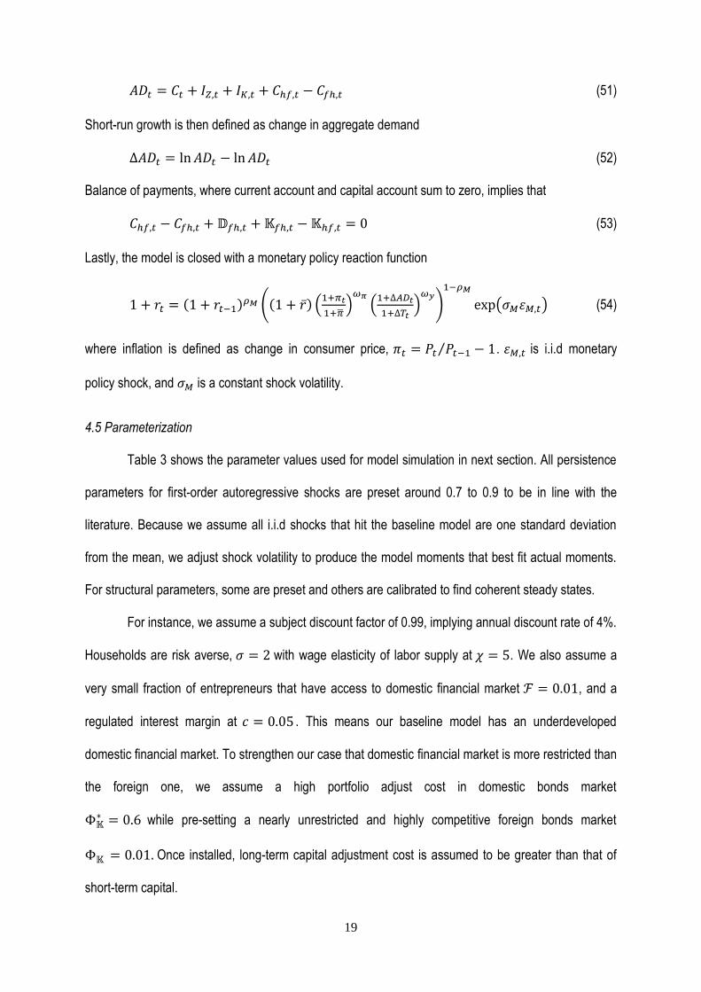
𝐴𝐷𝑡 = 𝐶𝑡 + 𝐼𝑍,𝑡 + 𝐼𝐾,𝑡 + 𝐶ℎ𝑓,𝑡 − 𝐶𝑓ℎ,𝑡 (51)

Short-run growth is then defined as change in aggregate demand

Δ𝐴𝐷𝑡 = ln𝐴𝐷𝑡 − ln𝐴𝐷𝑡 (52)

Balance of payments, where current account and capital account sum to zero, implies that

𝐶ℎ𝑓,𝑡 − 𝐶𝑓ℎ,𝑡 +𝔻𝑓ℎ,𝑡 +𝕂𝑓ℎ,𝑡 −𝕂ℎ𝑓,𝑡 = 0 (53)

Lastly, the model is closed with a monetary policy reaction function

1 + 𝑟𝑡 = (1 + 𝑟𝑡−1)𝜌𝑀 ((1 + �̅�) (

1+𝜋𝑡

1+�̅�)𝜔𝜋(1+∆𝐴𝐷𝑡

1+∆𝑇𝑡)𝜔𝑦)

1−𝜌𝑀

exp(𝜎𝑀휀𝑀,𝑡) (54)

where inflation is defined as change in consumer price, 𝜋𝑡 = 𝑃𝑡 𝑃𝑡−1⁄ − 1. 휀𝑀,𝑡 is i.i.d monetary

policy shock, and 𝜎𝑀 is a constant shock volatility.

4.5 Parameterization

Table 3 shows the parameter values used for model simulation in next section. All persistence

parameters for first-order autoregressive shocks are preset around 0.7 to 0.9 to be in line with the

literature. Because we assume all i.i.d shocks that hit the baseline model are one standard deviation

from the mean, we adjust shock volatility to produce the model moments that best fit actual moments.

For structural parameters, some are preset and others are calibrated to find coherent steady states.

For instance, we assume a subject discount factor of 0.99, implying annual discount rate of 4%.

Households are risk averse, 𝜎 = 2 with wage elasticity of labor supply at 𝜒 = 5. We also assume a

very small fraction of entrepreneurs that have access to domestic financial market ℱ = 0.01, and a

regulated interest margin at 𝑐 = 0.05 . This means our baseline model has an underdeveloped

domestic financial market. To strengthen our case that domestic financial market is more restricted than

the foreign one, we assume a high portfolio adjust cost in domestic bonds market

Φ𝕂∗ = 0.6 while pre-setting a nearly unrestricted and highly competitive foreign bonds market

Φ𝕂 = 0.01. Once installed, long-term capital adjustment cost is assumed to be greater than that of

short-term capital.

20

Lastly, the parameter values for short-term capital share 𝛼, and labor productivity in capital

goods sectors are calibrated to attain arbitrage condition (46) in steady state, depreciation rates for

short-term and long-term capital to meet equivalence of net marginal return in Eq. (47), and share of

capital outflows in total foreign bonds held to clear the balance of payments (53).

[INSERT TABLE 3 HERE]

Table 4 reports simulated moments compared with actual moments for Korea, Malaysia,

Thailand, and the Philippines on average. The statistics on actual moments are adopted from Aguiar

and Gopinath (2007). Overall, given a simple production structure and trade linkage in the model, while

it is reasonable to observe some anomalies, the model reasonably produces volatility, autocorrelation,

and cross-correlation that replicate at best and partially account for at worst the actual moments. For

instance, simulated short-run growth volatility at 1.771 approximates the actual one at 1.865. So does

the ratio between consumption volatility and aggregate demand volatility. The simulated ratio is 1.209,

slightly higher than actual ratio of 1.16. Besides, cyclical movements of simulated aggregate demand

has autocorrelation coefficient of 0.715 that is close to the actual coefficient of 0.848. Simulated cross-

correlation coefficients for consumption and investment, respectively, and aggregate demand also

substantially account for the actual cross-correlation coefficients.

[INSERT TABLE 4 HERE]

5. Asymmetric growth effect: The composition of investment and credit constraints

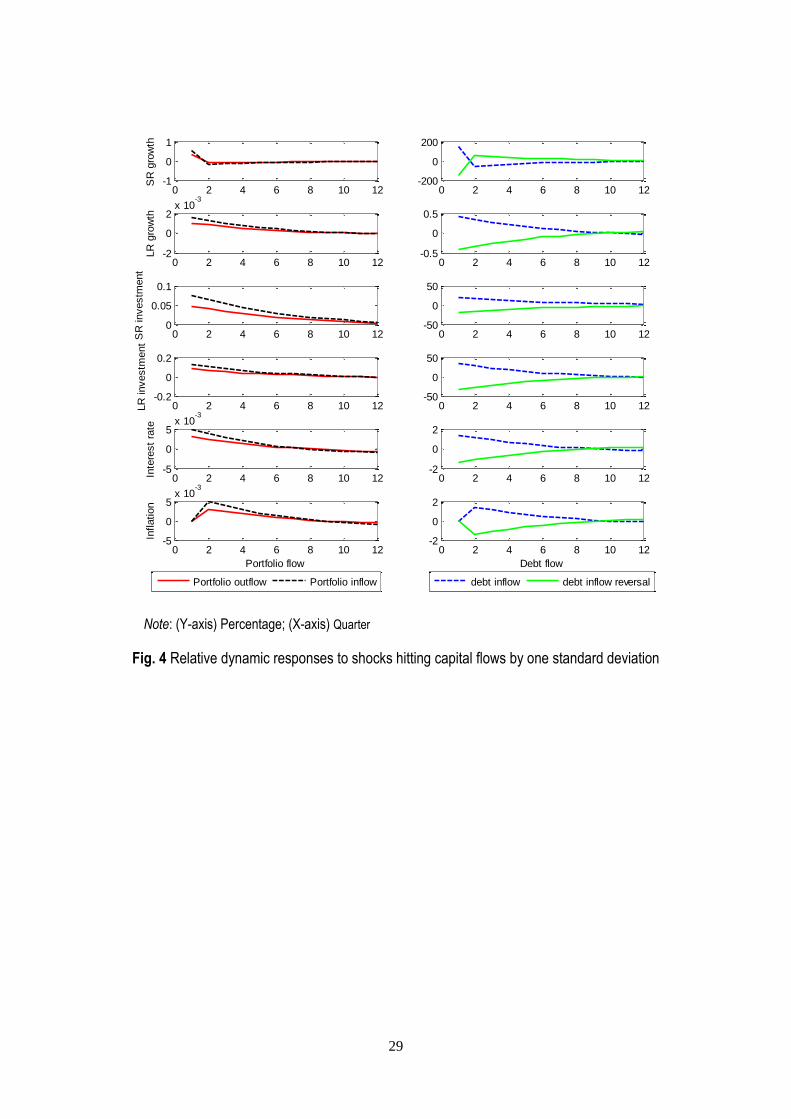
In this section, we would observe how the quantitative model economy responds to shocks

hitting portfolio capital inflows and outflows, debt inflows, and debt inflows reversal. Figure 4 illustrates

dynamic responses of short-run and long-run growth, short-term and long-term investment, interest rate,

and consumer price inflation rates relative to one standard deviation shock that hit those capital flows.

Relative impulse responses facilitate our understanding on how the economy may react differently in

magnitude and direction in responding to shocks to different types of capital flows.

21

[INSERT FIGURE 4 HERE]

Overall, there is no asymmetric long-run growth effect of capital flows when shocks hitting

capital flows are small. We observe trivial responses of long-run growth toward portfolio capital flows. In

addition, inflation, interest rate, and short-term investment also barely respond to portfolio capital flows,

both in and out. Interestingly, a stronger response of long-term investment doesn’t translate into greater

long-run growth rates. Responses of the economy are much stronger when facing debt flow shocks. In

particular, debt inflows raise long-run growth whereas debt inflows reversal takes a toll on the long-run

growth. However, responses are symmetric.

By thinking through our model, it is not unreasonable to obtain relative dynamic responses as

depicted in Figure 4. Without hitting arbitrage condition, asymmetry would not kick in following capital

inflows. On the flipside, without crashing the entrepreneur’s creditworthiness that causes liquidity

constraint to bind, long-run growth would not collapse as a consequence of capital outflows. In this

respect, small shock to portfolio capital flows would leave no mark on long-run growth.

At the same time, symmetric growth effect of debt flows can be interpreted jointly through the

lens of endogenous long-run trend, aggregate total factor productivity equation, arbitrage condition, and

endogenous probability of securing foreign loans. A positive shock to debt inflows expands the amount

of loans available for long-term capital accumulation, lifting long-run trend and hence aggregate TFP.

As a result, frontier of arbitrage condition is raised, which allows positive long-run growth of debt inflows

to take effect. Law of diminishing return, however, ensures that growth effects die off over time. In

contrast, debt inflow reversal cut backs cheaper foreign loans available for long-term investment,

resulting in immediate fall in long-run growth. However, reduction in long-term capital stock implies a

greater marginal return that makes long-term investment remains profitable even when it is financed by

more expensive domestic loans. As a result, long-run growth recovers over time.

5.1 Implication of large and persistence shocks hitting capital flows

22

Against this conjecture, it is possible to observe the emergence of asymmetry in growth effects

when shocks hitting portfolio capital flows are large and persistent. But large and persistent debt inflow

reversals are likely to only amplify responses of the economy without instigating asymmetry. We

conduct another exercise by hitting the model economy with shocks of four standard deviations over

zero mean. The large debt inflow reversal by four standard deviations is especially interesting as it fits

the key defining characteristics of a sudden stop: a sharp, sudden reversal in international capital flows

(Calvo et al. 2006, 2008). That means large shock to portfolio capital outflows is not a sudden stop

incidence because no reversal of flow takes place. We make the shock persistent by setting a near

unit-root autocorrelation coefficient for capital flows shock, 𝜌𝕂 = 𝜌𝕂∗ = 𝜌𝔻 = 0.99.

[INSERT FIGURE 5 HERE]

Figure 5 depicts relative impulse responses of the economy to large and persistent shocks

hitting capital flows. It is apparent that asymmetry in growth comes on-stream for portfolio capital flows.

While both short-run and long-run growth barely responds to large and persistent capital inflows shocks,

long-run growth drops by nearly 0.1% and short-run growth falls by about 30%. Meanwhile, falls in

growth, investment, interest rate, and inflation below trend are amplified when there is large and

persistent debt inflows reversal. Nevertheless, as inferred earlier, there is no mark of asymmetry.

5.2 Role of imperfect financial market

Is there a role for imperfect domestic financial market in instigating asymmetric growth effect of

capital flows? Would the dynamic responses be different if domestic financial market is equally

competitive and advanced as foreign financial market without financial repression? We undertake the

last exercise by setting ℱ = 1 and 𝑐 = 0, respectively. The former implies that all credit-financed

long-term investment would contribute to long-run growth perhaps due to unrestricted access to credit

market for the entrepreneurs, or because of more advanced monitoring device from the financial

intermediaries that ensures all borrowers are incentivized to carry the productive plan as proposed. The

23

latter implies an equally competitive domestic financial market, as now lending rates are equalized

across countries, 𝑟𝐿,𝑡∗ = 𝑟𝐿,𝑡.

[INSERT FIGURE 6 HERE]

Figure 6 illustrate relative dynamic responses under baseline case, “ℱ = 1” case, and “𝑐 = 0”

case when the economy is hit by large and persistent capital flow shocks. Three interesting

observations stand out. First, financial market development in the sense that domestic entrepreneurs

have greater access to credit market and that moral hazard incidence can be minimized due to more

advanced monitoring device is critical to make the economy responsive to capital flows. As evidenced

in Figure 6, portfolio capital inflows can be favorable to long-run growth with meaningful magnitude,

although it doesn’t contribute to productive investments. Growth effect of debt inflows is also amplified.

This finding in a way corroborates existing literature that found benign growth effects of capital inflows

conditional to the existence of strong and good institutions (see, for instance, Alfraso et al., 2007;

Bekaert et al., 2005; Friedrich et al., 2013; Kyaw and MacDonald, 2009; Masten et al., 2008). However,

it should be noted that while greater access to credit market implies greater chances for the

entrepreneurs, the ugly flipside holds true as it also implies more severe shakeup to the economy in the

face of greater collapse in credit-financed investments when capital flows retreat. In other words,

deeper and liberalized financial market is not a foolproof guarantee for the economy to escape financial

fragility stirred by the wreak-havocking sudden stops (Ranciere et al., 2006).

Second, the asymmetry survives. Although greater financial depth strengthens the favorable

effects of capital inflows on growth, so does the unfavorable growth effect of capital outflows. Lastly,

eliminating domestic interest rate control when the entrepreneurs already have access to cheaper

foreign credits has no impact on how the economy responds to capital flow shocks. It looks like a

“pseudo” Pareto improvement in the sense that it harms no one but it benefits no one as well.

24

6. Conclusion

When financial liberalization with unrestricted capital flows was promoted as the recipe for

economic development in developing countries in the 1990s, the promise was largely grounded on

untested theoretical good will. With the benefit of hindsight, it is now determined that the output gain to

capital inflows is largely elusive. However, we are constantly reminded by the lessons from the Asian

financial crisis of 1997/98, as well as the global financial crisis of 2008, that abrupt capital outflows can

easily wreak havoc on the economy.

This paper contributes to the literature with respect to empirical evidence and the underlying

mechanism. By using an asymmetric Granger causality test on a sample of Asian countries, this paper

for the first time finds statistically significant empirical evidence showing that while capital inflows hardly

Granger-cause economic growth, capital outflows Granger-cause economic downturn. To explain this

finding, we construct a small open-economy model that incorporates different compositions of

investment and endogenous nonlinear credit constraint. Of different types of investments, only long-

term investment contributes to long-run growth. Arbitrage condition between short-term and long-term

investments hence sets an upper bound, over which further capital inflows would not incentivize long-

term investments and hence are decoupled from long-run growth.

Because long-term investment need financing that is endogenous to the entrepreneur’s

creditworthiness, nonlinear credit constraint triggers debt-deflation process once capital outflows

deteriorate the entrepreneur’s creditworthiness, which, in turn, reinforcing cutbacks in foreign financing.

Nevertheless, debt-deflation process is not explosive in the model, as the resultant increasing marginal

return would make long-term investment profitable even when it is financed by the more expensive

domestic credits. Our mechanism of asymmetry survives different level of financial development.

References Alfaro, L., Kalemli-Ozcan, S., Volosovych, V., 2007. Capital flows in a globalized world: The role of

policies and institutions. In Sebastian, E. (ed.) Capital Controls and Capital Flows in Emerging

25

Economies: Policies, Practices, and Consequences. National Bureau of Economics Research, University of Chicago Press.

Aghion, P., Angeletos, G.-M., Banerjee, A., Manova, K., 2010. Volatility and growth: Credit constraints and the composition of investment. Journal of Monetary Economics 57, 246-265.

Aghion, P., Howitt, P.W., 2008. The Economics of Growth. MIT Press. Bekaert, G., Harvey, C.R., Lundblad, C., 2005. Does financial liberalization spur growth? Journal of

Financial Economics 77, 3-55. Bordo, M.D., Meissner, C.M., 2006. The role of foreign currency debt in financial crises: 1880-1913

versus 1972-1997. Journal of Banking & Finance 30, 3299-3329. Bordo, M.D., Meissner, C.M., Stuckler, D., 2010. Foreign currency debt, financial crises and economic

growth: A long-run view. Journal of International Money and Finance 29, 642-665. Calvo, G.A., Izquierdo, A., Loo-Kung R., 2006. Relative price volatility under Sudden Stops: the

relevance of balance sheet effects. Journal of International Economics 69, 231-254. Calvo, G.A., Izquierdo, A., Mejia L-F., 2008. Systemic Sudden Stops: the relevance of balance-sheet

effects and financial integration. NBER Working Paper No. 14026. Eichengreen, B., Leblang, D., 2003. Capital account liberalization and growth: Was Mr. Mahathir right?

International Journal of Finance and Economics 8, 205-224. Elliott, G., Rothenberg, T.J., Stock, J.H., 1996. Efficient tests for an autoregressive unit root.

Econometrica 64(4), 813-836. Friedrich, C., Schnabel, I., Zettelmeyer, J., 2012. Financial integration and growth: Why is emerging

Europe different? Journal of International Economics, doi:10.1016/j.jinteco.2012.07.003. Gamra, S.B., 2009. Does financial liberalization matter for emerging East Asian economies growth?

Some new evidence. International Review of Economics and Finance 18, 392-403. Granger, C.W.J., Yoon, G., 2002. Hidden cointegration. Royal Economic Society Annual Conference

2002, Royal Economic Sociey. Gourinchas, P., Jeanne, O., 2006. The elusive gains from international financial integration. Review of

Economic Studies 73(3), 715-741. Gospodinov, N., Herrera, A.M., Pesavento, E., 2013. Unit roots, cointegration and pre-testing in VAR

models. Mimeo, Concordia University. Hatemi-J, A., 2003. A new method to choose optimal lag order in stable and unstable VAR models.

Applied Economics Letter 10(3), 135-137. Hatemi-J, A., 2008. Forecasting properties of a new method to choose optimal lag order in stable and

unstable VAR models. Applied Economics Letter 15(4), 239-243. Hatemi-J, A., 2012. Asymmetric causality tests with an application. Empirical Economics 43(1), 447-456. Jeanne, O., Subramanian, A., Williamson, J., 2012. Who Needs to Open the Capital Account? Peterson

Institute for International Economics. Klein, M.W., Olivei, G.P., 2008. Capital account liberalization, financial depth, and economic growth.

Journal of International Money and Finance 27, 861-875. Korinek, A., Mendoza, E., 2014. From sudden stops to Fisher deflation: Quantitative theory and policy.

Annual Review of Economics 6, 299-332. Kose, M.A., Prasad, E.S., Wei, S.-J., Rogoff, K., 2009a. Financial globalization: A reappraisal. IMF Staff

Papers 56(1), 8-62. Kose, M.A., Prasad, E.S., Terrones, M.E., 2009b. Does openness to international financial flows raise

productivity growth? Journal of International Money and Finance 28, 554-580. Kyaw, K.S, MacDonald, R., 2009. Capital flows and growth in developing countries: A dynamic panel

data analysis. Oxford Development Studies 37(2), 101-122. Masten, A.B., Coricelli, F., Masten, I., 2008. Non-linear growth effects of financial development: Does

financial integration matter? Journal of International Money and Finance 27, 295-313. Prasad, E.S., Rajan, R.G., Subraminian, A., 2007. Foreign capital and economic growth. Brooking

Papers on Economic Activity 1, 153-230.

26

Ranciere, R., Tornell, A., Westermann, F., 2006. Decomposing the effects of financial liberalization: Crises vs. growth. Journal of Banking & Finance 30, 3331-3348.

Tille, C., 2012. Sailing through this storm? Capital flows in Asia during the crisis. Pacific Economic Review 17(3), 467-488.

Toda, H.Y., Yamamoto, T., 1995. Statistical inference in vector autoregressions with possibly integrated processes. Journal of Econometrics 66, 225-250.

Notes: -CA/GDP: current account as a share of GDP; KA/GDP: capital account as a share of GDP; DRGDPPC: Per capita real GDP growth rate. Declining –CA/GDP and KA/GDP indicates capital outflows, and vice versa.

Fig. 1 Asymmetric relationship between capital flows and economic growth

-12

-10

-8

-6

-4

-2

0

2

4

-30

-20

-10

0

10

20

30

40

50

1980 1985 1990 1995 2000 2005 2010

-CA/GDP KA/GDP DRGDPPC

-3

-2

-1

0

1

2

3

4

5

6

-20

-15

-10

-5

0

5

10

15

20

25

1980 1985 1990 1995 2000 2005 2010

-12

-8

-4

0

4

8

12

16

-100

-80

-60

-40

-20

0

20

40

1980 1985 1990 1995 2000 2005 2010

-6

-5

-4

-3

-2

-1

0

1

2

-30

-20

-10

0

10

20

30

40

50

1980 1985 1990 1995 2000 2005 2010

-16

-12

-8

-4

0

4

8

12

-40

-30

-20

-10

0

10

20

30

1980 1985 1990 1995 2000 2005 2010

-20

-16

-12

-8

-4

0

4

8

12

16

-50

-40

-30

-20

-10

0

10

20

30

40

1980 1985 1990 1995 2000 2005 2010

-12

-8

-4

0

4

8

12

16

20

-20

-15

-10

-5

0

5

10

15

20

1980 1985 1990 1995 2000 2005 2010

-40

-30

-20

-10

0

10

20

30

40

-20

-15

-10

-5

0

5

10

15

20

1980 1985 1990 1995 2000 2005 2010

-15

-10

-5

0

5

10

15

-40

-30

-20

-10

0

10

20

1980 1985 1990 1995 2000 2005 2010

Philippines Singapore Thailand

Malays iaKoreaJapan

India IndonesiaChina

27

Fig. 2 Time plots of per capita real gross domestic product for selected Asian countries

6.0

6.5

7.0

7.5

8.0

8.5

1980 1985 1990 1995 2000 2005 2010

5.8

6.0

6.2

6.4

6.6

6.8

7.0

7.2

1980 1985 1990 1995 2000 2005 2010

6.0

6.4

6.8

7.2

7.6

8.0

1980 1985 1990 1995 2000 2005 2010

9.6

10.0

10.4

10.8

11.2

1980 1985 1990 1995 2000 2005 2010

8.0

8.5

9.0

9.5

10.0

1980 1985 1990 1995 2000 2005 2010

7.8

8.0

8.2

8.4

8.6

8.8

9.0

1980 1985 1990 1995 2000 2005 2010

6.6

6.8

7.0

7.2

7.4

7.6

1980 1985 1990 1995 2000 2005 2010

8.8

9.2

9.6

10.0

10.4

10.8

1980 1985 1990 1995 2000 2005 2010

6.8

7.2

7.6

8.0

8.4

1980 1985 1990 1995 2000 2005 2010

China India Indonesia

Japan Korea Malay sia

Philippines Singapore Thailand

28

0

5

10

15

20

25

0.0

0.5

1.0

1.5

2.0

2.5

3.0

1985 1990 1995 2000 2005 2010

-24

-20

-16

-12

-8

-4

0

-.6

-.5

-.4

-.3

-.2

-.1

.0

1985 1990 1995 2000 2005 2010

0

2

4

6

8

10

12

0.0

0.4

0.8

1.2

1.6

1985 1990 1995 2000 2005 2010

-10

-8

-6

-4

-2

0

-.6

-.5

-.4

-.3

-.2

-.1

.0

1985 1990 1995 2000 2005 2010

0

5

10

15

20

25

30

0.0

0.5

1.0

1.5

2.0

2.5

3.0

1985 1990 1995 2000 2005 2010

-40

-30

-20

-10

0

-1.50

-1.25

-1.00

-0.75

-0.50

-0.25

0.00

1985 1990 1995 2000 2005 2010

0

2

4

6

8

10

12

0.0

0.4

0.8

1.2

1.6

2.0

1985 1990 1995 2000 2005 2010

-16

-12

-8

-4

0

-1.0

-0.8

-0.6

-0.4

-0.2

0.0

1985 1990 1995 2000 2005 2010

0

10

20

30

40

0.0

0.4

0.8

1.2

1.6

2.0

2.4

2.8

1985 1990 1995 2000 2005 2010

-50

-40

-30

-20

-10

0

-1.0

-0.8

-0.6

-0.4

-0.2

0.0

1985 1990 1995 2000 2005 2010

0

20

40

60

80

0.0

0.5

1.0

1.5

2.0

1985 1990 1995 2000 2005 2010

-100

-80

-60

-40

-20

0

-1.0

-0.8

-0.6

-0.4

-0.2

0.0

1985 1990 1995 2000 2005 2010

0

10

20

30

40

0.0

0.4

0.8

1.2

1.6

1985 1990 1995 2000 2005 2010

-50

-40

-30

-20

-10

0

-1.2

-1.0

-0.8

-0.6

-0.4

-0.2

0.0

1985 1990 1995 2000 2005 2010

0

10

20

30

40

50

60

0.0

0.5

1.0

1.5

2.0

2.5

1985 1990 1995 2000 2005 2010

-100

-80

-60

-40

-20

0

-.6

-.5

-.4

-.3

-.2

-.1

.0

1985 1990 1995 2000 2005 2010

0

10

20

30

40

50

0.0

0.5

1.0

1.5

2.0

2.5

1985 1990 1995 2000 2005 2010

-60

-50

-40

-30

-20

-10

0

-1.0

-0.8

-0.6

-0.4

-0.2

0.0

1985 1990 1995 2000 2005 2010

-CA/GDP KA/GDP RGDPPC

𝒞ℱ+/𝑌+ 𝒞ℱ−/𝑌− 𝒞ℱ+/𝑌+ 𝒞ℱ−/𝑌−

China India

Indonesia Japan

Korea Malaysia

Philippines Singapore

Thailand

Notes: 𝒞ℱ denotes capital flows proxied by –CA/GDP and KA/GDP, 𝑌 denotes per capita real GDP (RGDPPC). The sign + indicates cumulative positive sum and – indicates cumulative negative sum.

Fig. 3 Cumulative positive and negative sum of capital flow and economic growth

29

Note: (Y-axis) Percentage; (X-axis) Quarter

Fig. 4 Relative dynamic responses to shocks hitting capital flows by one standard deviation

0 2 4 6 8 10 12-1

0

1S

R g

row

th

0 2 4 6 8 10 12-2

0

2x 10

-3

LR

gro

wth

0 2 4 6 8 10 120

0.05

0.1

SR

investm

ent

0 2 4 6 8 10 12-0.2

0

0.2

LR

investm

ent

0 2 4 6 8 10 12-5

0

5x 10

-3

Inte

rest

rate

0 2 4 6 8 10 12-5

0

5x 10

-3

Inflation

Portfolio flow

0 2 4 6 8 10 12-200

0

200

0 2 4 6 8 10 12-0.5

0

0.5

0 2 4 6 8 10 12-50

0

50

0 2 4 6 8 10 12-50

0

50

0 2 4 6 8 10 12-2

0

2

0 2 4 6 8 10 12-2

0

2

Debt flow

Portfolio outflow Portfolio inflow debt inflow debt inflow reversal

30

Note: (Y-axis) Percentage; (X-axis) Quarter

Fig. 5 Relative dynamic responses to near unit root shocks hitting capital flows by four s.d.

0 2 4 6 8 10 12-50

0

50

SR

gro

wth

0 2 4 6 8 10 12-0.1

0

0.1

LR

gro

wth

0 2 4 6 8 10 12-5

0

5

SR

investm

ent

0 2 4 6 8 10 12-10

0

10

LR

investm

ent

0 2 4 6 8 10 12-0.5

0

0.5

Inte

rest

rate

0 2 4 6 8 10 12-0.5

0

0.5

Inflation

Portfolio flow

Portfolio outflow Portfolio inflow

0 2 4 6 8 10 12-500

0

500

0 2 4 6 8 10 12-1

0

1

0 2 4 6 8 10 12-50

0

50

0 2 4 6 8 10 12-50

0

50

0 2 4 6 8 10 12-5

0

5

0 2 4 6 8 10 12-5

0

5

Debt flow

debt inflow debt inflow reversal

31

Note: (Y-axis) Percentage; (X-axis) Quarter. Baseline refers to those in Fig. 5, f=1 implies unrestricted assess of entrepreneurs to domestic credit market, and spread=0 means unregulated domestic lending rate

Fig. 6 Implication of imperfect credit market

0 5 10 15-100

0

100

SR

gro

wth

0 5 10 15-2

0

2

0 5 10 15-1000

0

1000

0 5 10 15-10

-5

0

LR

gro

wth

0 5 10 150

0.2

0.4

0 5 10 150

50

100

0 5 10 15-4

-2

0

SR

Investm

ent

0 5 10 150

0.1

0.2

0 5 10 1510

20

30

0 5 10 15-10

-5

0

LR

Investm

ent

0 5 10 150

0.1

0.2

0 5 10 150

50

100

0 5 10 15

-0.4

-0.2

0

Inte

rest

rate

0 5 10 150

0.01

0.02

0 5 10 150

5

0 5 10 15-0.5

0

0.5

Inflation

Capital outflow

0 5 10 15-0.02

0

0.02

Capital inflow

0 5 10 15-5

0

5

Debt inflow

0 5 10 15-1000

0

1000

0 5 10 15-100

-50

0

0 5 10 15-30

-20

-10

0 5 10 15-100

-50

0

0 5 10 15

-4

-2

0

0 5 10 15-5

0

5

Debt inflow reversal

baseline f=1 spread=0

32

Table 1 Results of asymmetric causality tests

China India Indonesia Japan Korea Malaysia Philippines Singapore Thailand

Ho: CF+≠>RGDPC+

Wstat 0.395 3.05* 1.932 0.328 2.266 1.207 0.45 0.014 1.295

Bootstrap CV 1% 8.52 7.525 15.003 9.937 7.916 7.834 8.629 7.169 8.531

Bootstrap CV 5% 4.244 4.391 9.641 4.72 4.214 4.38 4.45 4.079 4.771

Bootstrap CV 10% 2.902 3.026 7.222 3.101 2.955 3 2.967 2.947 3.313

Ho: CF+≠>RGDPC-

Wstat 5.984* 3.945* 30.598*** 3.947 16.616*** 0.355 1.120 0.014 0.576

Bootstrap CV 1% 12.507 8.491 18.375 12.357 11.846 7.629 7.776 7.169 7.48

Bootstrap CV 5% 7.14 4.575 10.385 7.249 7.018 4.206 4.277 4.079 4.154

Bootstrap CV 10% 5.285 3.161 7.797 5.299 5.24 2.94 2.997 2.947 2.933

Ho: CF- ≠>RGDPC+

Wstat 0.292 0.310 0.049 0.001 2.11 0.251 3.908 0.053 0.592

Bootstrap CV 1% 12.921 8.608 9.43 10.005 15.062 8.69 12.163 10.709 9.338

Bootstrap CV 5% 5.232 4.366 4.6 4.986 5.972 4.331 7.031 4.241 4.659

Bootstrap CV 10% 3.04 3.044 2.94 3.217 3.403 2.835 5.126 2.658 3.001

Ho: CF- ≠>RGDPC-

Wstat 11.733** 1.087 23.027*** 0.489 50.180*** 19.65*** 15.351*** 1.375 22.513***

Bootstrap CV 1% 13.055 8.646 14.529 7.912 24.873 15.898 9.751 10.128 15.944

Bootstrap CV 5% 7.477 4.376 5.098 4.318 10.731 5.721 4.972 4.503 8.362

Bootstrap CV 10% 5.466 2.897 2.992 2.903 6.854 3.229 3.186 2.928 5.749

China India Indonesia Japan Korea Malaysia Philippines Singapore Thailand

Ho: RGDPC+≠>CF+

Wstat 0.888 0.281 2.068 2.159 1.293 0.656 0.175 0.319 0.045

Bootstrap CV 1% 8.545 8.188 17.146 9.66 9.261 8.058 7.968 8.823 8.477

Bootstrap CV 5% 4.478 4.374 10.429 4.51 4.733 4.558 4.279 4.638 4.592

Bootstrap CV 10% 3.064 3.02 7.815 2.94 3.221 3.087 2.951 3.196 3.197

Ho: RGDPC+≠>CF-

Wstat 0.003 0.121 0.613 0.383 1.008 5.231** 0.276 0.319 0.505

Bootstrap CV 1% 11.665 8.168 10.027 8.581 11.524 10.568 12.649 8.823 10.016

Bootstrap CV 5% 5.139 4.342 4.889 4.548 4.839 4.521 7.262 4.638 4.709

Bootstrap CV 10% 3.118 2.895 3.073 2.985 2.922 2.906 5.282 3.196 3.038

Ho: RGDPC- ≠>CF+

Wstat 7.641** 0.001 1.017 6.715* 0.909 0.614 0.187 2.966 0.001

Bootstrap CV 1% 12.813 8.351 14.358 12.762 11.664 7.921 7.981 12.432 8.231

Bootstrap CV 5% 7.257 4.387 8.736 7.075 6.915 4.293 4.521 7.417 4.6

Bootstrap CV 10% 5.262 3.064 6.691 5.284 5.171 2.928 3.053 5.577 3.33

Ho: RGDPC- ≠>CF-

Wstat 0.091 2.156 0.021 1.665 0.305 2.541 0.047 0.066 1.499

Bootstrap CV 1% 11.807 10.261 9.828 8.602 12.898 8.205 8.168 8.427 12.785

Bootstrap CV 5% 7.015 4.827 4.305 4.485 7.782 4.364 4.305 4.271 7.658

Bootstrap CV 10% 5.229 3.074 2.812 3.039 5.828 2.915 2.912 2.923 5.64

Notes: RGDPC denotes per capita real GDP (in log) and CF denotes capital flow proxied by current account as a share of GDP (-CA/GDP). The sign + denotes cumulative positive shock which indicates capital inflow and positive economic growth, whereas the sign – denotes negative cumulative shock that implies capital outflow and negative economic growth, respectively. Wstat and CV stand for Wald statistics and critical value, respectively. The denotation ≠> indicates “does not Granger cause”. ***, **, *, respectively, denote 1%, 5%, and 10% level of significance.

33

Table 2 Further results of asymmetric causality test

China India Indonesia Japan Korea Malaysia Philippines Singapore Thailand

Ho: CF+≠>RGDPC+

Wstat 0.303 4.082* 0.101 0.362 3.172* 3.358* 0.087 2.825 4.769

Bootstrap CV 1% 8.547 8.634 8.42 8.267 7.845 7.648 8.395 16.028 13.577

Bootstrap CV 5% 4.265 4.332 4.36 4.62 4.224 4.242 4.47 10.023 7.849

Bootstrap CV 10% 2.88 3.01 2.986 3.13 2.894 2.94 3.078 7.591 5.852

Ho: CF+≠>RGDPC-

Wstat 0.591 0.635 17.322** 2.160 21.103*** 0.861 1.135 2.825 0.378

Bootstrap CV 1% 8.465 8.585 17.957 14.567 12.034 7.549 7.705 16.028 7.11

Bootstrap CV 5% 4.554 4.602 10.099 7.768 6.999 4.055 4.119 10.023 4.106

Bootstrap CV 10% 3.11 3.081 7.575 5.406 5.293 2.849 2.936 7.591 2.898

Ho: CF- ≠>RGDPC+

Wstat 0.224 1.082 0.000 0.604 2.038 0.441 11.021** 0.048 0.198

Bootstrap CV 1% 13.555 8.908 12.478 9.896 13.67 9.518 11.472 11.184 12.634

Bootstrap CV 5% 5.379 4.591 4.638 4.749 6.03 4.42 6.768 4.214 4.759

Bootstrap CV 10% 3.062 3.066 2.926 3.159 3.547 2.856 5.044 2.675 2.821

Ho: CF- ≠>RGDPC-

Wstat 9.531*** 1.847 59.601*** 0.047 38.262*** 29.147*** 27.108*** 1.315 25.076***

Bootstrap CV 1% 8.411 8.074 23.463 9.207 22.671 18.006 10.511 9.328 15.66

Bootstrap CV 5% 4.265 4.226 8.625 4.521 9.688 6.734 4.946 4.624 8.063

Bootstrap CV 10% 2.929 2.862 5.559 2.961 6.068 3.696 3.08 3.02 5.7

China India Indonesia Japan Korea Malaysia Philippines Singapore Thailand

Ho: RGDPC+≠>CF+

Wstat 2.011 3.322* 6.603** 1.377 3.141* 1.035 0.634 5.139 0.768

Bootstrap CV 1% 8.868 8.199 9.402 8.928 8.808 8.138 8.394 18.086 12.956

Bootstrap CV 5% 4.567 4.147 4.536 4.572 4.623 4.436 4.539 10.893 7.594

Bootstrap CV 10% 3.078 2.825 3.014 3.084 3.13 3.135 3.187 8.29 5.626

Ho: RGDPC+≠>CF-

Wstat 0.009 0.031 0.126 0.99 0.343 3.549* 0.220 5.139 0.129

Bootstrap CV 1% 13.212 8.253 10.865 8.779 10.935 10.16 11.567 18.086 11.087

Bootstrap CV 5% 5.37 4.35 4.706 4.474 4.663 4.42 7.035 10.893 4.854

Bootstrap CV 10% 3.037 2.927 2.945 3.045 2.897 2.827 5.081 8.29 2.966

Ho: RGDPC- ≠>CF+

Wstat 1.594 0.457 1.254 2.544 1.030 0.312 0.463 0.107 0.132

Bootstrap CV 1% 8.113 8.68 13.515 13.737 11.766 7.894 7.785 8.853 7.999

Bootstrap CV 5% 4.418 4.548 8.301 7.437 6.934 4.321 4.311 4.668 4.596

Bootstrap CV 10% 3.03 3.146 6.326 5.186 5.177 3.024 2.976 3.152 3.265

Ho: RGDPC- ≠>CF-

Wstat 0.072 0.062 2.081 0.329 0.301 1.226 0.038 0.005 1.447

Bootstrap CV 1% 8.73 9.471 13.701 8.847 12.979 7.772 7.886 8.204 12.876

Bootstrap CV 5% 4.456 4.587 7.967 4.386 7.612 4.123 4.375 4.336 7.716

Bootstrap CV 10% 3.006 3.022 5.864 2.92 5.743 2.822 2.905 2.969 5.644

Notes: Capital account as a share of GDP is used as proxy for capital flow (CF). RGDPC denotes per capita real GDP (in log). The sign + denotes cumulative positive shock which indicates capital inflow and positive economic growth, whereas the sign – denotes negative cumulative shock that implies capital outflow and negative economic growth, respectively. Wstat and CV stand for Wald statistics and critical value, respectively. The denotation ≠> indicates “does not Granger cause”. ***, **, *, respectively, denote 1%, 5%, and 10% level of significance.

34

Table 3 Parameterization

Parameters Shocks

Pre-set Calibrated Pre-set

𝛽 0.99 𝛼 0.4885 Shock persistence

𝜎 2 𝛿𝕂 0.202 𝜌𝑎 0.85

𝜒 5 𝛿𝐾 0.04 𝜌𝐻 0.7

𝑐 0.05 𝛿𝑍 0.015 𝜌𝐾 0.9

ℱ 0.01 𝜃𝐾 0.7762 𝜌𝑍 0.9

𝜛 150 𝜃𝑍 1.228 𝜌𝕂 0.9

𝛿𝕂∗ 0.1 𝜌𝕂

∗ 0.9

𝛿𝔻 0.1 𝜌𝔻∗ 0.9

Φ𝕂 0.01 Volatility

Φ𝕂∗ 0.6 𝜎𝑎 0.0001

Φ𝔻 0.01 𝜎𝐻 0.005

Φ𝐾 0.1 𝜎𝐾 0.01

Φ𝑍 0.3 𝜎𝑍 0.2

𝛾 0.7 𝜎𝕂 0.2

𝜑 1.5 𝜎𝕂∗ 0.2

𝜌𝑀 0.7 𝜎𝔻∗ 0.2

𝜔𝜋 1.5 𝜎𝑀 0.0001

𝜔𝑦 0.03125 𝜎𝑀∗ 0.00001

Table 4 A comparison between actual and simulated moments

Data

Model Simulation

𝜎(𝐴𝐷) 3.24 1.971

𝜎(Δ𝐴𝐷) 1.865 1.771

𝜌(𝐴𝐷) 0.848 0.715

𝜌(Δ𝐴𝐷) 0.33 -0.054

𝜎(𝐶)/𝜎(𝐴𝐷) 1.16 1.209

𝜎(𝐼)/𝜎(𝐴𝐷) 3.868 0.219

𝜌(𝐶, 𝐴𝐷) 0.78 0.382

𝜌(𝐼, 𝐴𝐷) 0.828 0.505 Notes: Data is computed based on business cycles statistics for South Korea, Malaysia, the Philippines, and Thailand reported in Aguiar and Gopinath (2007). Simulated series are de-trended using HP filter at 𝜆 = 1600.