Asset price and wealth dynamics in a financial market with heterogeneous agents

ARTICLE IN PRESS

Journal of Economic Dynamics & Control 30 (2006) 1755–1786

0165-1889/$ -

doi:10.1016/j

�CorrespoD. Anghera

E-mail ad

gardini@eco

www.elsevier.com/locate/jedc

Asset price and wealth dynamics in a financialmarket with heterogeneous agents

Carl Chiarellaa, Roberto Diecib,�, Laura Gardinic

aSchool of Finance and Economics, University of Technology Sydney P.O. Box 123 Broadway NSW 2007,

AustraliabDipartimento di Matematica per le Scienze Economiche e Sociali, University of Bologna,

I-40126 Bologna, ItalycIstituto di Scienze Economiche, University of Urbino, I-61029 Urbino, Italy

Received 30 September 2004; accepted 4 October 2005

Available online 8 May 2006

Abstract

This paper considers a discrete-time model of a financial market with one risky asset and

one risk-free asset, where the asset price and wealth dynamics are determined by the

interaction of two groups of agents, fundamentalists and chartists. In each period each group

allocates its wealth between the risky asset and the safe asset according to myopic expected

utility maximization, but the two groups have heterogeneous beliefs about the price change

over the next period: the chartists are trend extrapolators, while the fundamentalists expect

that the price will return to the fundamental. We assume that investors’ optimal demand for

the risky asset depends on wealth, as a result of CRRA utility. A market maker is assumed to

adjust the market price at the end of each trading period, based on excess demand and on

changes of the underlying reference price. The model results in a nonlinear discrete-time

dynamical system, with growing price and wealth processes, but it is reduced to a stationary

system in terms of asset returns and wealth shares of the two groups. It is shown that the long-

run market dynamics are highly dependent on the parameters which characterize agents’

behaviour as well as on the initial condition. Moreover, for wide ranges of the parameters a

(locally) stable fundamental steady state coexists with a stable ‘non-fundamental’ steady state,

or with a stable closed orbit, where only chartists survive in the long run: such cases require the

see front matter r 2006 Elsevier B.V. All rights reserved.

.jedc.2005.10.011

nding author. Universita degli Studi di Bologna, Facolta di Economia del Polo di Rimini, Via

22, I-47900 Rimini, Italy. Tel.: +39 541 434140.

dresses: [email protected] (C. Chiarella), [email protected] (R. Dieci),

n.uniurb.it (L. Gardini).

www.elsevier.com/locate/jedc

dx.doi.org/10.1016/j.jedc.2005.10.011

mailto:[email protected]

mailto:[email protected]

ARTICLE IN PRESS

C. Chiarella et al. / Journal of Economic Dynamics & Control 30 (2006) 1755–17861756

numerical and graphical investigation of the basins of attraction. Other dynamic scenarios

include periodic orbits and more complex attractors, where in general both types of agents

survive in the long run, with time-varying wealth fractions.

r 2006 Elsevier B.V. All rights reserved.

JEL classification: C61; D84; G12

Keywords: Heterogeneous agents; Financial market dynamics; Wealth dynamics; Coexisting attractors

1. Introduction

In recent years, several models of asset price dynamics based on the interaction ofheterogeneous agents have been proposed (Day and Huang, 1990; Kirman, 1991;Brock and LeBaron, 1996; Brock and Hommes, 1998; Lux, 1998; Gaunersdorfer,2000; Chiarella and He, 2001a, 2003; Farmer and Joshi, 2002; Chen and Yeh, 2002;Hommes et al., 2005, to quote only a few). This heterogeneous agent literature canbe classified as either theoretically or computationally oriented in general, and hasbeen extensively discussed in two recent surveys by Hommes (2006) and LeBaron(2006). In particular, Hommes’ survey discusses the state of the art of analyticallytractable heterogeneous agent models,1 whereas LeBaron’s survey discussesextensively related work on computational heterogeneous agent-based models infinance. The common setup of several heterogeneous agent models in finance ischaracterized by a stylized market with one risky asset and one riskless asset, and themain focus is on the effect of heterogeneous beliefs and trading rules on the dynamicsof the price of the risky security. Most models however, some of which allow the sizeof the different groups of agents to vary according to the relative profitability of theadopted trading rules, are of necessity rather difficult to treat analytically. Chiarellaet al. (2002) have developed a two-dimensional discrete time model of asset pricedynamics that contains the essential elements of the heterogeneous agents paradigmwhilst still remaining mathematically tractable. In that paper, a financial market witha risky asset and an alternative asset has been assumed, consisting of two types oftraders, fundamentalists and chartists, and of a market maker, who adjusts the pricein each period depending on excess demand. In Chiarella et al. (2002), as well as inmost studies on the interaction of heterogeneous agents, the evolution of agents’wealth and its effect on price dynamics is left in the background; indeed, in thosepapers the underlying assumptions about agents’ portfolio allocation follow theframework of Brock and Hommes (1998), where optimal demand for the risky assetis independent on agents’ wealth, as a result of the assumption of constant absoluterisk aversion (CARA) utility functions.

In general these assumptions are unrealistic:2 a more realistic framework, whereinvestors’ optimal decisions depend on their wealth, has been proposed and analyzed

1Some of which are closely related to the one considered in the present paper.2See e.g. Levy et al. (2000) and Campbell and Viceira (2002), for a discussion of this point.

ARTICLE IN PRESS

C. Chiarella et al. / Journal of Economic Dynamics & Control 30 (2006) 1755–1786 1757

through numerical simulation by Levy et al. (1994, 1995). This framework isconsistent with the assumption of constant relative risk aversion (CRRA) utilityfunctions. More recently, Chiarella and He (2001b, 2002) have proved analyticallythe existence of multiple steady states in financial market models with heterogeneousagents and CRRA utility: in these papers, the main focus is on the existence andstability of multiple equilibria as a function of the trend traders’ extrapolation rate.

The present paper aims to contribute to the development and analysis of suchmodels, by analyzing the dynamics of asset price and agents’ wealth within afundamentalists/chartists framework similar to the one developed in Chiarella et al.(2002). In addition, we allow for a growing dividend process and a trend in thefundamental price of the risky asset. As a consequence, the model that we developresults in price and wealth being determined simultaneously over time, as in realmarkets, which gives rise to interdependent growing wealth and price processes.3 Inorder to obtain analytical results about the dynamics of the growing system, and todiscuss the role played by the key parameters and by the initial conditions, the non-stationary model is reformulated in terms of returns and wealth shares and reducedto a stationary system. Though in the framework of the present paper agents are notallowed to switch among different groups according to the relative profitability ofthe adopted trading rules, the time-varying wealth shares modify the impact of thetwo groups on the market demand, thus determining endogenously time-varyingweights of fundamentalists and chartists. As a consequence, differently from thefundamentalists–chartists CARA framework developed in Chiarella et al. (2002), weare now able to characterize the equilibria and the other kinds of asymptoticbehaviour in terms of long-run evolution of the wealth proportions.

The structure of the paper is as follows. Section 2 presents the general frameworkof the model. In particular, Section 2.1 derives the asset demand of a generic agent,as a function of his/her beliefs about the risky return, in a framework consistent withCRRA utility. Section 2.2 derives a benchmark notion of fundamental solution,which plays a role in fundamentalist expectations formation. Section 2.3 describesthe schemes used by fundamentalists and chartists to form and revise theirexpectations, and thus provides a specification of the demand function of eachgroup. Section 2.4 describes how demands are aggregated by a market maker, whosets the price depending on excess demand. Section 3 presents the resulting nonlineardynamical system for the dynamic evolution of fundamental value and price, agents’expected returns, and wealth of the two groups. In Section 3.1 this is reduced to astationary map in terms of actual and expected capital gain of the risky asset,fundamental to price ratio, and wealth shares of the two groups. The steady statesare determined and their properties are discussed in Section 3.2. Numericalexploration of the global behaviour and discussion of the main dynamic scenarios,as well as stochastic simulations are contained in Section 4. Section 5 concludes.Mathematical details are provided in the Appendices.

3Related papers that investigate non-stationary heterogeneous agents models with growing dividends

given by a geometric random walk, are Brock and Hommes (1997b) and Hommes (2002).

ARTICLE IN PRESS


2. The model

We consider a discrete-time model of a financial market with one risky asset andone riskless asset, two types of interacting agents, fundamentalists and chartists

(denoted by j 2 ff ; cg), and a market maker. The starting point is Chiarella et al.(2002), whose antecedents are Chiarella (1992), Beja and Goldman (1980), andZeeman (1974).

Each group has CRRA utility of wealth function. We denote, at time t, by OðjÞt thewealth of group j and by Z

ðjÞt the fraction of wealth that agent-type j invests in the

risky asset. We also denote by Pt and P�t the market price and the fundamental priceof the risky asset, respectively, by r ðr40Þ the (constant) risk-free rate, by Dt the(random) dividend, while Dt=Pt�1 is the dividend yield in period t. The fundamental‘reference’ price P�t , which will be defined in Section 2.2, is assumed to be known tothe fundamentalists and to the market maker.

As we shall see in the next section, the fraction ZðjÞt is independent of the wealth

level under our assumptions, and therefore the demand OðjÞt ZðjÞt for the risky asset is

proportional to the wealth level OðjÞt . The number of agents within each group isassumed fixed. Given that traders of the same group are assumed to have the samebeliefs, risk aversion and trading strategies, the proportion of wealth invested in therisky asset at each point in time will be the same for all the agents of the same group.This implies that the distribution of wealth among the agents of the same type has noinfluence on the dynamics, but only total wealth for each group matters. As aconsequence, we can normalize to one the number of agents of each group, and useindifferently the terms agent j or agent-type j (or group j). Wealth of agent-type j

evolves according to

OðjÞtþ1 ¼ OðjÞt þ OðjÞt ZðjÞt

Ptþ1 þDtþ1 � Pt

Pt

� �þ OðjÞt ð1� Z

ðjÞt Þr

¼ OðjÞt 1þ rþ ZðjÞt

Ptþ1 þDtþ1 � ð1þ rÞPt

Pt

� �� , ð1Þ

where ðPtþ1 þDtþ1 � ð1þ rÞPtÞ=Pt represents the excess return in period tþ 1.

2.1. Asset demand

Each agent is assumed to have a CRRA (power) utility of wealth function of thetype

uðjÞðOÞ ¼

1

1� lðjÞðO1�lðjÞ � 1Þ ðlðjÞa1Þ;

lnðOÞ ðlðjÞ ¼ 1Þ;

8><>:

where O40 and the parameter lðjÞ40 represents the relative risk aversion coefficient.

Denote by EðjÞt , Var

ðjÞt the ‘beliefs’ of agent-type j about expectation and variance.

Each agent seeks the investment fraction ZðjÞt maximizing the expected utility of

ARTICLE IN PRESS


wealth at time tþ 1, that is maxZðjÞtEðjÞt ½uðjÞðOðjÞtþ1Þ�. As is well known, an analytical

exact solution to this problem can be obtained only under very particularassumptions.4 Chiarella and He (2001b) derive the following approximate optimalsolution (which we adopt in the present paper):

ZðjÞt ¼

EðjÞt ½ðPtþ1 þDtþ1 � PtÞ=Pt � r�

lðjÞVarðjÞt ½ðPtþ1 þDtþ1 � PtÞ=Pt � r�

¼EðjÞt ½rtþ1 þ dtþ1 � r�

lðjÞVarðjÞt ½rtþ1 þ dtþ1 � r�

,

where rtþ1 � ðPtþ1 � PtÞ=Pt and dtþ1 � Dtþ1=Pt denote the capital gain and the

dividend yield, respectively. Therefore, ZðjÞt is proportional to agent j’s ‘risk-adjusted’

expected excess return.

2.2. Fundamental price

Following the framework of Brock and Hommes (1998), Appendix A derivesendogenously a reference notion of ‘fundamental solution’, as a long-run marketclearing price path which would be obtained under homogeneous beliefs aboutexpected excess return. Furthermore, this price is assumed to satisfy a long-runstability condition, namely the ‘no-bubbles’ condition.

Here we focus on the particular case of zero net supply of shares,5 where thefundamental price can be derived from the ‘no-arbitrage’ equation

Et½Ptþ1 þDtþ1� ¼ ð1þ rÞPt. (2)

As it is well known, the unique solution to the expectational equation (2) whichsatisfies the no-bubbles transversality condition, limk!þ1 Et½Ptþk�=ð1þ rÞk ¼ 0, isgiven by

Pt ¼ P�t �X1k¼1

Et½Dtþk�

ð1þ rÞk. (3)

In particular, in the case of an i.i.d. dividend process fDtg with Et½Dtþk� ¼ D, k ¼

1; 2; . . . ; the fundamental solution (3) is constant, given by P�t ¼ P� ¼ D=r, while inthe case of a dividend process described by6

Et½Dtþk� ¼ ð1þ fÞkDt; k ¼ 1; 2; . . . , (4)

with 0pfor, the fundamental solution is given by

P�t ¼ ð1þ fÞDt=ðr� fÞ. (5)

We will use the latter specification of the dividend process: as one can easily checkthis implies that the fundamental evolves over time according to7

Et½P�tþ1� ¼ ð1þ fÞP�t (6)

4See e.g. Campbell and Viceira (2002).5In doing so we follow Brock and Hommes (1998) and Chiarella and He (2001a). Appendix A discusses

the general case of positive net supply.6This case is known in the finance literature as ‘Gordon growth model’.7Which reduces to Et½P

�tþ1� ¼ P�t in the particular case f ¼ 0.

ARTICLE IN PRESS


and that along the fundamental path the expected dividend yield and the capital gainare given, respectively, by

Et½dtþ1� � Et

Dtþ1

P�t

� �¼ r� f; Et½rtþ1� � Et

P�tþ1 � P�tP�t

� �¼ f.

In the next section, we introduce heterogeneity into the model, by taking the viewthat agents form heterogeneous, time-varying beliefs about the first and secondmoment of returns, though they are assumed to share the same beliefs aboutexpected dividends (according to (4)).

2.3. Heterogeneous beliefs

The two groups differ in the way they form and update their beliefs about the pricechange over the next period. We introduce heterogeneous beliefs both about theexpectation and the variance of the excess return.

The fundamentalists believe that the price will return to the (known) fundamentalin the future, so that their expected price change is given by

Eðf Þt ½Ptþ1 � Pt� ¼ E

ðf Þt ½P

�tþ1 � P�t � þ ZðP�t � PtÞ

¼ fP�t þ ZðP�t � PtÞ.

The fundamentalist rule is based on the expected change in the underlyingfundamental and includes a correction term, proportional to the difference betweenfundamental and current price, which depends on their beliefs about the speed ofmean reversion (captured by the parameter Z, 0oZo1). We also assume thatfundamentalist conditional variance is constant over time, Var

ðf Þt ½rtþ1 þ dtþ1� ¼ s2f .

The fundamentalist investment fraction in the risky asset thus becomes

Zðf Þt ¼

1

Pt

ZðP�t � PtÞ þ fP�t þ ð1þ fÞDt � rPt

lðf Þs2f. (7)

The chartists do not rely on the knowledge of the fundamental price. Instead, theybehave as trend followers and try to extrapolate into the future the movements ofpast prices. Therefore, the chartists’ conditional expected price change evolves overtime according to a weighted average (with geometrically declining weights) of pastcapital gains, which results in the adaptive rule

mðcÞt � E

ðcÞt ½rtþ1� ¼ E

ðcÞt

Ptþ1 � Pt

Pt

� �

¼ ð1� cÞmðcÞt�1 þ c

Pt � Pt�1

Pt�1

� �¼ ð1� cÞm

ðcÞt�1 þ crt,

where the parameter c; 0oco1, represents the weight given to the most recent pricechange.

We introduce a risk-adjustment mechanism into the demand function of thechartists, by assuming that they have time-varying beliefs about the variance of theexcess return. Precisely, we assume that their beliefs about the second moment are

ARTICLE IN PRESS


state dependent, in the sense that chartists expect that market risk increases when theexpected excess return moves away (above or below) from ‘normal’ levels, e.g. duringphases of booms and crashes. Put differently, in our model the chartists behave asspeculators who try to exploit the current price trends. However, they perceive therisk that a market characterized, for instance, by very high expected returns mightcollapse. This leads to our assumption of state-dependent beliefs about risk.A simple way to model this idea (similar to Chiarella et al., 2002), is to assume thatat each time step the estimated variance s2c;t � Var

ðcÞt ½rtþ1 þ dtþ1 � r� depends posi-

tively on the magnitude of the expected excess return, i.e. s2c;t ¼ vðxtÞ, xt �

EðcÞt ½rtþ1 þ dtþ1 � r�, with v0ðxÞ40 (v0ðxÞo0) for x40 (xo0), and where vð0Þ40

represents a minimum level of variance corresponding to the ‘normal’ case of zeroexpected excess return. Note that under this simplifying assumption the chartistinvestment fraction in the risky asset turns out to depend only on the expected excessreturn, i.e. Z

ðcÞt ¼ ZðcÞðxtÞ ¼ xt=ðl

ðcÞvðxtÞÞ. In spite of this risk-adjustment mechan-ism, we assume however that chartists are more sensitive to the chance of higherreturns than to the related risk, and that variations of vðxÞ are not large enough as tocompromise the monotonic shape of the function ZðcÞðxÞ: namely, we assume that thefunction vðxÞ is ‘inelastic’, jv0ðxÞjovðxÞ=jxj.8 In particular, we adopt a functionZðcÞðxÞ with an increasing and bounded S-shaped graph, whose slope levels off as themagnitude jxtj of the expected excess return increases. We use the following two-parameter specification

ZðcÞt ¼

gytanhfyxtg ¼

gytanhfy½mðcÞt þ ð1þ fÞDt=Pt � r�g, (8)

where g, y40, which provides a sufficiently flexible formulation. Indeed theparameter g ¼ 1=ðlðcÞvð0ÞÞ,9 which is inversely related to chartists’ risk aversion,represents the slope of the chartist investment fraction ZðcÞðxÞ computed for x ¼ 0(see Fig. 1a), that we will call strength of chartist demand; moreover, for a given g,the parameter y governs the position of the floor and the ceiling for the fraction ofwealth invested in the risky asset (see Fig. 1b). Fig. 1c represents the ‘implied’variance function vðxÞ corresponding to the case with y ¼ 50 and vð0Þ ¼ 0:0025.

8Note that xv0ðxÞovðxÞ is equivalent to dZðcÞ=dx40. Moreover, our assumptions about vðxÞ imply also

dZðcÞ=dxo ZðcÞðxÞ=x. Note also that the assumed qualitative properties do not prevent vðxÞ from being

convex, as is the case of the function used in our model. Of course, other convex functions – for instance

the simple quadratic function vðxÞ ¼ vð0Þ þ ax2, a40 – may lead to non-monotonic demand functions. We

are grateful to one of the referees for having raised the question of the connection between the qualitative

behaviour of vðxÞ and that of ZðcÞðxÞ.9Our choice of a hyperbolic tangent to represent the S-shaped chartist investment in the risky asset

implies an estimated variance given by vðxÞ ¼ vð0Þyx= tanhfyxg, where vð0Þ � limx!0 vðxÞ, whose graph is

represented in Fig. 1c. In this case the function vðxÞ is strictly convex and approaches asymptotically the

straight lines of equation f ðxÞ ¼ �vð0Þyx as x!1. Of course other specifications are possible, for

example an unbounded S-shaped function could also be consistent with our assumptions about the

variance vðxÞ. Analytical and numerical study of the model with alternative specifications show that what

really matters in order to get the key dynamic features of the model are the assumed qualitative properties

of vðxÞ and ZðcÞðxÞ.

ARTICLE IN PRESS

Fig. 1. The assumed sigmoid shape of the chartist investment fraction in the risky asset ZðcÞðxÞ ¼

ðg=yÞ tanhfyxg, as a function of the expected excess return, for different values of the parameter g ¼1=ðlðcÞvð0ÞÞ (a) and y (b). An example of the ‘implied’ variance vðxÞ is represented in (c).


We note that because of Eq. (5) we obtain ð1þ fÞDt ¼ ðr� fÞP�t , so that thedemand functions (7) and (8) can be rewritten, respectively, as

Zðf Þt ¼ðZþ rÞðP�t � PtÞ=Pt

lðf Þs2f; Z

ðcÞt ¼

gytanhfy½mðcÞt þ ðr� fÞP�t =Pt � r�g.

2.4. Price setting rule

Price adjustments are operated by a market maker, who is assumed to know thefundamental reference price.10 The market maker clears the market at the end ofperiod t by taking an off-setting long or short position and announces the nextperiod price as a function of agents’ excess demand and expected changes in thereference price. In the general case, the assumed price setting rule of the marketmaker will be given by

Ptþ1 � Pt ¼ EðmÞt ½P

�tþ1 � P�t � þ PtHtðN

Dt �NS

t Þ, (9)

where EðmÞt ½P

�tþ1 � P�t � ¼ E

ðf Þt ½P

�tþ1 � P�t � ¼ fP�t is the market maker’s expected

change in the underlying fundamental, NDt ¼ ðO

ðf Þt Z

ðf Þt þ OðcÞt Z

ðcÞt Þ=Pt is the total

10The use of the market maker mechanism to clear the market in fundamentalist–chartist models goes

back at least to Beja and Goldman (1980) and Day and Huang (1990).

ARTICLE IN PRESS


agents’ demand at time t (number of shares), NSt denotes the supply of shares at time

t, and it is assumed in general that Htð�Þ is a strictly increasing function, withHtð0Þ ¼ 0. In Eq. (9) the term PtHtðN

Dt �NS

t Þ represents the price change due toexcess demand, while E

ðmÞt ½P

�tþ1 � P�t � captures the price adjustment due to news

about the underlying fundamental price. The price setting rule (9) is a very stylizedone, which however can be justified in the light of recent theoretical and empiricalwork on financial market microstructure (see e.g. the survey in Madhavan, 2000): forinstance, Madhavan and Smidt (1993) develop a market maker model of a financialmarket with informed and uninformed traders, where the specialist seeks tomaximize his/her final wealth by choosing both the price quote and the trade. It isfound that under the optimal specialist’s policy, the change in the price quote hasthree components: (i) a term depending on order imbalances, (ii) a term whichcaptures market maker’s revision of beliefs about the underlying asset value and (iii) aterm depending on the desired change in inventories. In our stylized framework, inorder to keep the model simple and to focus on the behaviour of heterogeneoustraders, we only consider the impact of excess demand and changes in the underlyingasset value; the role of inventories is left in the background, though of course thisrepresents an important aspect of the market maker decision problem in real markets.

Notice that total agents’ demand NDt (number of shares) can be rewritten as

NDt ¼ ZtOt=Pt, where Ot ¼ Oðf Þt þ OðcÞt is the total wealth and Zt � ðO

ðf Þt Z

ðf Þt þ

OðcÞt ZðcÞt Þ=Ot is the fraction of total wealth invested in the risky asset at time t.

Denoting by Qt � NSt Pt=Ot the value of the supply of shares as a fraction of total

agents’ wealth, we also obtain NSt ¼ QtOt=Pt, so that ND

t �NSt ¼ ðZt �QtÞOt=Pt.

We model the market maker rule as independent of the level of growing prices andwealth (so that it is not affected by the level of Ot=Pt) i.e. we assume

HtðNDt �NS

t Þ ¼ HðZt �QtÞ,

where H is strictly increasing with Hð0Þ ¼ 0. We will adopt the linear specificationHðZt �QtÞ ¼ bðZt �QtÞ, b40. In particular, in the case of zero net supply we getHðZt �QtÞ ¼ HðZtÞ ¼ bZt.

3. The dynamical system

Under the assumed stochastic processes of the dividends and fundamental price,the dynamics of the model will be given in general by a ‘noisy’ nonlinear dynamicalsystem. In this paper, we focus on the dynamics of the ‘deterministic skeleton’ of themodel, i.e. we assume that dividends evolve in a deterministic way according to theircommonly shared expected value (Section 4.1). Some numerical simulations of astochastic version of the model are contained in Section 4.2. The deterministicdynamics can be summarized as

Ptþ1 ¼ Pt þ fP�t þ PtbZt, (10)

mðcÞtþ1 ¼ ð1� cÞm

ðcÞt þ c½ðPtþ1 � PtÞ=Pt�, (11)

ARTICLE IN PRESS


P�tþ1 ¼ ð1þ fÞP�t , (12)

OðjÞtþ1 ¼ OðjÞt 1þ rþ ZðjÞt


Pt

� �� ; j 2 ff ; cg, (13)

where

Ot ¼ Oðf Þt þ OðcÞt ; Zt ¼ ðOðf Þt Z


ðcÞt Þ=Ot,

Zðf Þt ¼ðZþ rÞðP�t � PtÞ=Pt

lðf Þs2f; Z

ðcÞt ¼

gytanhfy½mðcÞt þ ðr� fÞP�t =Pt � r�g.

Although the system results in general in growing price11 and wealth processes, it ispossible to obtain a stationary12 system in terms of capital gain rtþ1 � ðPtþ1 � PtÞ=Pt,fundamental/price ratio yt � P�t =Pt, and wealth shares of fundamentalists andchartists w

ðjÞt � OðjÞt =Ot, j 2 ff ; cg, with w

ðcÞt ¼ ð1� w

ðf Þt Þ.

Moreover, we denote by

gðjÞtþ1 ¼ rþ Z

ðjÞt


Pt

� �; j 2 ff ; cg,

the growth rate of wealth of agent-type j, and by

gtþ1 ¼ rþ Zt


Pt

� �¼ w

ðf Þt gðf Þtþ1 þ ð1� w

ðf Þt Þg

ðcÞtþ1

the rate of growth of total wealth. Notice also that (in the deterministic skeleton of themodel) the actual excess return on the risky asset in period tþ 1 can be rewritten as


Pt

¼Ptþ1 � Pt

Pt

þðr� fÞP�t

Pt

� r

¼ rtþ1 þ ðr� fÞyt � r.

In particular, a dynamic equation for the wealth shares can be obtained by rewritingthe wealth recurrence equations (1) for j 2 ff ; cg as

wðjÞtþ1Otþ1 ¼ w

ðjÞt Otð1þ g

ðjÞtþ1Þ. (14)

By summing up Eq. (14) for j 2 ff ; cg, and recalling that wðf Þtþ1 þ w

ðcÞtþ1 ¼ 1 we obtain

Otþ1 ¼ Ot½wðf Þt ð1þ g

ðf Þtþ1Þ þ w

ðcÞt ð1þ g

ðcÞtþ1Þ� ¼ Otð1þ gtþ1Þ,

and finally Eq. (14) becomes for j ¼ f

wðf Þtþ1 ¼ w

ðf Þt ð1þ g

ðf Þtþ1Þ

Ot

Otþ1¼

wðf Þt ð1þ g

ðf Þtþ1Þ

ð1þ gtþ1Þ.

11Note however that the underlying deterministic model, in the particular case f ¼ 0, reduces to the case

of constant fundamental.12The term stationary here is used in the sense that we reduce the growing system to a form which admits

steady state solutions.

ARTICLE IN PRESS


3.1. The map

The changes of variables performed in the previous section allow us to rewrite theoriginal dynamical model in terms of the state variables rt, yt, m

ðcÞt , w

ðf Þt . The time

evolution of the stationary system is given by the iteration of the following nonlinearmap T : ðr; y;mðcÞ;wðf ÞÞ7�!ðr0; y0;mðcÞ0;wðf Þ0Þ, where the symbol 0 denotes the unit timeadvancement operator:

T :

r0 ¼ fyþ bZ;

y0 ¼ yð1þ fÞ=ð1þ r0Þ;

mðcÞ0 ¼ ð1� cÞmðcÞ þ cr0;

wðf Þ0 ¼ wðf Þ½1þ rþ Zðf Þðr0 þ ðr� fÞy� rÞ�=½1þ rþ Zðr0 þ ðr� fÞy� rÞ�;

8>>>><>>>>:

(15)

where

Zðf Þ ¼ðZþ rÞðy� 1Þ

lðf Þs2f; ZðcÞ ¼

gytanh½yðmðcÞ þ ðr� fÞy� rÞ�,

Z ¼ wðf ÞZðf Þ þ ð1� wðf ÞÞZðcÞ.

Although in (15) we have four dynamic variables, the map T could in fact beimmediately rewritten as a three-dimensional map, given that r0 is a function of y,mðcÞ and wðf Þ. However, we keep the higher dimensional form (15), in order toconsider explicitly the behaviour of the dynamic variable r (capital gain).

3.2. Steady states

We now discuss the existence and stability of the steady states of the map T. Asproven in Appendix B, the map (15) has two types of steady states, that we denote byfundamental steady states and by non-fundamental steady states, respectively. Themap also presents other important trapping13 subsets of the phase space.

Fundamental steady states: Fundamental steady states are characterized by

y ¼ 1,

r ¼ mðcÞ ¼ f,

wðf Þ ¼ wðf Þ; wðf Þ 2 ½0; 1�,

i.e. by the price being at the fundamental (Pt ¼ P�t , for any t) and growing at thefundamental rate f, and by zero excess demand, Z ¼ 0. The long-run wealthdistribution ðwðf Þ; 1� wðf ÞÞ at a fundamental steady state may be given, in general, byany wðf Þ 2 ½0; 1�. This means that a continuum of steady states exists:14 numericalsimulations of the dynamical system in Section 4.1 show that the steady state wealth

13A subset X of the phase space is trapping if it is mapped into itself, i.e. TðX Þ � X .14They are located in a one-dimensional subset (a straight line) of the phase space.

ARTICLE IN PRESS


distribution which is reached by the system in the long run depends on the initialcondition.

Non-fundamental steady states: For particular ranges of the parameters othersteady states exist, coexisting with the fundamental ones. They are characterized by

y ¼ 0,

wðf Þ ¼ 0,

r ¼ mðcÞ ¼ r,

where r solves

r=b ¼ ðg=yÞ tanh½yðr� rÞ�. (16)

It can be shown (see Appendix B) that the non-fundamental growth rates r whichcome out as positive solutions of (16) are higher than the risk free rate r (and thushigher than the fundamental growth rate f). Non-fundamental steady states are thuscharacterized by the price growing faster than the fundamental, r ¼ mðcÞ ¼ r4r4f,the fundamental/price ratio converging to 0, y ¼ 0, i.e. limt!1Pt=P�t ¼ þ1, themarket dominated by chartists, wðf Þ ¼ 0, and a permanent positive excess demandZ ¼ ZðcÞ ¼ ðg=yÞ tanh½yðr� rÞ�40. Numerical simulations show that, for wideranges of the parameters, a locally attracting non-fundamental steady state exists.Of course, the existence of such attracting non-fundamental equilibrium, where theprice increasingly deviates from the fundamental and the fundamentalist wealthbecomes negligible, represents a situation which cannot be sustained in the long run:this is a sort of ‘deterministic bubble’ which lasts forever. This dynamic outcome isdue, first of all, to the deterministic nature of the model being considered here, whichrepresents the ‘skeleton’ of a stochastic dynamic model. Once noise is added to thesystem, the behaviour of price and wealth becomes more realistic and often phases ofbooms alternate with phases of crashes in an unpredictable way, with a complexevolution of prices and wealth shares (see Section 4.2). Second, the present model is apartial equilibrium model, where the permanent excess demand of over-optimisticchartists causes the asset price to grow faster than its fundamental, even in the caseof zero outside supply and zero ‘fundamental’ risk premium: the reason is that theexcess demand is assumed to be always satisfied by the market maker within thepresent model, without any constraint from the side of inventories. A further reasonmay be that in our simple framework agents’ consumption, and its effect on wealthdynamics, is not taken intoaccount.15 Nevertheless, the existence and stability ofsuch equilibria provides the important information that bubbles may start to developfor particular initial conditions and under particular sets of parameters.

Trapping sets: Further important trapping subsets of the phase space representthe cases where only fundamentalists (wðf Þ ¼ 1) or only chartists (wðf Þ ¼ 0) populatethe market.

15This is indeed an important issue, as recently stressed in a different framework by Hens and Schenk-

Hoppe (2006), who argue that the way consumption is modelled – or not modelled at all – affects the long-

run evolution of the wealth shares of agents with heterogeneous trading strategies.

ARTICLE IN PRESS


In the case wðf Þ ¼ 1 (the market dominated by the fundamentalists) the evolutionof the model is determined by the following map:

T ðf Þ :r0 ¼ fyþ bZðf Þ;


(

where the dynamic equation for mðcÞ has been neglected given that it has no influenceon the dynamics of r and y. One can prove very easily (see Appendix B) that in thiscase the fundamental steady state is the only equilibrium characterized by non-negative growth rate of the price. Moreover, the model in this case can be rewrittenas a one-dimensional system, and the fundamental steady state is locally stable forsufficiently low expected speed of mean reversion ðZÞ, high risk aversion ðlðf ÞÞ, lowspeed of market reaction ðbÞ.

In the case wðf Þ ¼ 0 (the market dominated by the chartists) the dynamics aredriven by the map16

T ðcÞ :

r0 ¼ fyþ bZðcÞ;


mðcÞ0 ¼ ð1� cÞmðcÞ þ cr0:

8><>:

In this particular case it can be proven that (see again Appendix B):

�

1

1

sta

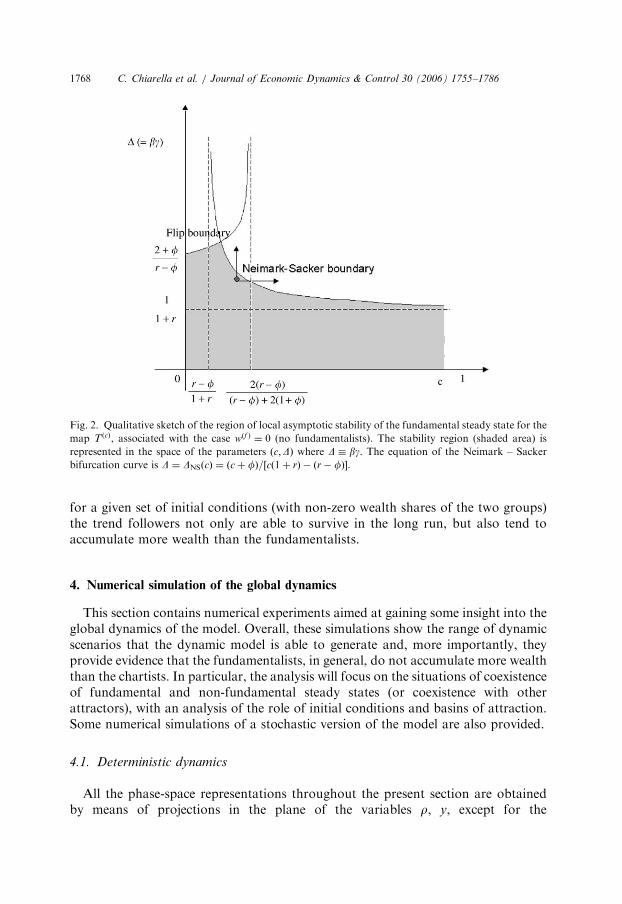
the ‘fundamental’ equilibrium y ¼ 1, r ¼ mðcÞ ¼ f, is locally asymptotically stablefor low values of c (strength of extrapolation), b (price reaction) and g (i.e. forhigh chartists’ risk aversion), as can be seen from the stability domain representedin Fig. 2;
� for higher values of c, b and g the fundamental steady state is no longer attracting.
As shown in Fig. 2, when D � bg or c are varied so that the bifurcation curve ofequation D ¼ DNSðcÞ ¼ ðcþ fÞ=½cð1þ rÞ � ðr� fÞ� is crossed from inside thestability region, then the steady state becomes unstable via a Neimark – Sackerbifurcation,17 which is followed by the appearance of a stable closed curve. Forparameter selections far from the Neimark – Sacker boundary, the systemconverges to an attracting limit cycle (with long-run fluctuations of the pricearound the fundamental) or to a non-fundamental equilibrium (with permanentand increasing deviation of the price away from the fundamental).

Numerical simulations show that the attractors of the map T ðcÞ (limit cycle, non-fundamental steady state) are in general attractors also for the map T, i.e. they canbe reached starting with w

ðf Þ0 40 as well. This fact has two implications. From the

mathematical point of view, this enhances the importance of the analysis of theparticular case w

ðf Þ0 ¼ 0, which proves very useful in understanding the dynamics of

the system in the general case. From the evolutionary point of view, this means that

6Which could be rewritten as a two-dimensional map.7We have numerical evidence of the supercritical nature of the Neimark – Sacker bifurcation, with a

ble limit cycle issuing from the bifurcated steady state.

ARTICLE IN PRESS

Fig. 2. Qualitative sketch of the region of local asymptotic stability of the fundamental steady state for the

map T ðcÞ, associated with the case wðf Þ ¼ 0 (no fundamentalists). The stability region (shaded area) is

represented in the space of the parameters ðc;DÞ where D � bg. The equation of the Neimark – Sacker

bifurcation curve is D ¼ DNSðcÞ ¼ ðcþ fÞ=½cð1þ rÞ � ðr� fÞ�.


for a given set of initial conditions (with non-zero wealth shares of the two groups)the trend followers not only are able to survive in the long run, but also tend toaccumulate more wealth than the fundamentalists.

4. Numerical simulation of the global dynamics

This section contains numerical experiments aimed at gaining some insight into theglobal dynamics of the model. Overall, these simulations show the range of dynamicscenarios that the dynamic model is able to generate and, more importantly, theyprovide evidence that the fundamentalists, in general, do not accumulate more wealththan the chartists. In particular, the analysis will focus on the situations of coexistenceof fundamental and non-fundamental steady states (or coexistence with otherattractors), with an analysis of the role of initial conditions and basins of attraction.Some numerical simulations of a stochastic version of the model are also provided.

4.1. Deterministic dynamics

All the phase-space representations throughout the present section are obtainedby means of projections in the plane of the variables r, y, except for the

ARTICLE IN PRESS


basins of attraction in Fig. 5 (where the initial conditions are taken in the planewðf Þ; y).

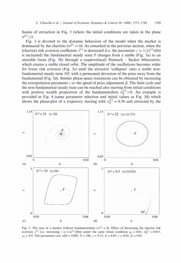
Fig. 3 is devoted to the dynamic behaviour of the model when the market isdominated by the chartists (wðf Þ ¼ 0). As remarked in the previous section, when the(chartist) risk aversion coefficient lðcÞ is decreased (i.e. the parameter g ¼ 1=ðlðcÞvð0ÞÞis increased) the fundamental steady state F changes from a stable (Fig. 3a) to anunstable focus (Fig. 3b) through a (supercritical) Neimark – Sacker bifurcation,which creates a stable closed orbit. The amplitude of the oscillations becomes widerfor lower risk aversion (Fig. 3c) until the attractor ‘collapses’ onto a stable non-fundamental steady state NF, with a permanent deviation of the price away from thefundamental (Fig. 3d). Similar phase-space transitions can be obtained by increasingthe extrapolation parameter c or the speed of price adjustment b. The limit cycle andthe non-fundamental steady state can be reached also starting from initial conditionswith positive wealth proportion of the fundamentalists w

ðf Þ0 40. An example is

provided in Fig. 4 (same parameter selection and initial values as Fig. 3d) whichshows the phase-plot of a trajectory starting with w

ðf Þ0 ¼ 0:56 and attracted by the

Fig. 3. The case of a market without fundamentalists ðwðf Þ ¼ 0Þ. Effect of decreasing the chartist risk

aversion lðcÞ (i.e. increasing g � 1=ðlðcÞvð0ÞÞ) under the same initial condition r0 ¼ 0:01, mðcÞ0 ¼ 0:015,

y0 ¼ 0:9. The parameters are: vð0Þ ¼ 0:002, y ¼ 100, c ¼ 0:25, b ¼ 0:05, r ¼ 0:02, f ¼ 0:01.

ARTICLE IN PRESS

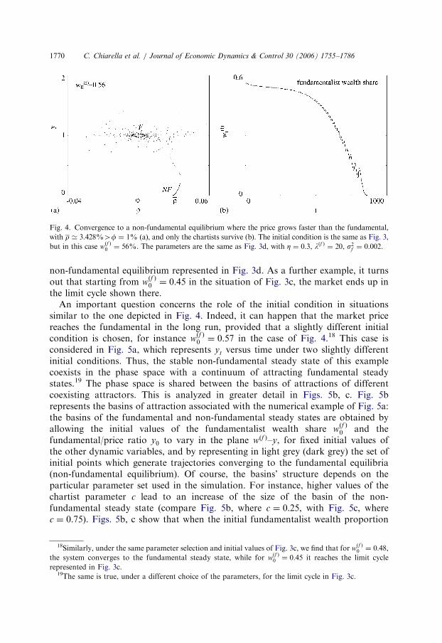
Fig. 4. Convergence to a non-fundamental equilibrium where the price grows faster than the fundamental,

with r ’ 3:428%4f ¼ 1% (a), and only the chartists survive (b). The initial condition is the same as Fig. 3,

but in this case wðf Þ0 ¼ 56%. The parameters are the same as Fig. 3d, with Z ¼ 0:3, lðf Þ ¼ 20, s2f ¼ 0:002.


non-fundamental equilibrium represented in Fig. 3d. As a further example, it turnsout that starting from w

ðf Þ0 ¼ 0:45 in the situation of Fig. 3c, the market ends up in

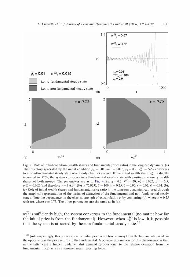
the limit cycle shown there.An important question concerns the role of the initial condition in situations

similar to the one depicted in Fig. 4. Indeed, it can happen that the market pricereaches the fundamental in the long run, provided that a slightly different initialcondition is chosen, for instance w

ðf Þ0 ¼ 0:57 in the case of Fig. 4.18 This case is

considered in Fig. 5a, which represents yt versus time under two slightly differentinitial conditions. Thus, the stable non-fundamental steady state of this examplecoexists in the phase space with a continuum of attracting fundamental steadystates.19 The phase space is shared between the basins of attractions of differentcoexisting attractors. This is analyzed in greater detail in Figs. 5b, c. Fig. 5brepresents the basins of attraction associated with the numerical example of Fig. 5a:the basins of the fundamental and non-fundamental steady states are obtained byallowing the initial values of the fundamentalist wealth share w

ðf Þ0 and the

fundamental/price ratio y0 to vary in the plane wðf Þ–y, for fixed initial values ofthe other dynamic variables, and by representing in light grey (dark grey) the set ofinitial points which generate trajectories converging to the fundamental equilibria(non-fundamental equilibrium). Of course, the basins’ structure depends on theparticular parameter set used in the simulation. For instance, higher values of thechartist parameter c lead to an increase of the size of the basin of the non-fundamental steady state (compare Fig. 5b, where c ¼ 0:25, with Fig. 5c, wherec ¼ 0:75). Figs. 5b, c show that when the initial fundamentalist wealth proportion

18Similarly, under the same parameter selection and initial values of Fig. 3c, we find that for wðf Þ0 ¼ 0:48,

the system converges to the fundamental steady state, while for wðf Þ0 ¼ 0:45 it reaches the limit cycle

represented in Fig. 3c.19The same is true, under a different choice of the parameters, for the limit cycle in Fig. 3c.

ARTICLE IN PRESS

Fig. 5. Role of initial condition (wealth shares and fundamental/price ratio) in the long-run dynamics. (a)

The trajectory generated by the initial condition r0 ¼ 0:01, mðcÞ0 ¼ 0:015, y0 ¼ 0:9, w

ðf Þ0 ¼ 56% converges

to a non-fundamental steady state where only chartists survive. If the initial wealth share wðf Þ0 is slightly

increased to 57%, the system converges to a fundamental steady state with positive stationary wealth

shares of both groups. The parameters are as in Fig. 4, i.e. Z ¼ 0:3, lðf Þ ¼ 20, s2f ¼ 0:002, lðcÞ ¼ 6:5,vð0Þ ¼ 0:002 (and therefore g ¼ 1=ðlðcÞvð0ÞÞ ’ 76:923), y ¼ 100, c ¼ 0:25, b ¼ 0:05, r ¼ 0:02, f ¼ 0:01. (b),(c) Role of initial wealth shares and fundamental/price ratio in the long-run dynamics, captured through

the graphical representation of the basins of attraction of the fundamental and non-fundamental steady

states. Note the dependence on the chartist strength of extrapolation c, by comparing (b), where c ¼ 0:25with (c), where c ¼ 0:75. The other parameters are the same as in (a).


wðf Þ0 is sufficiently high, the system converges to the fundamental (no matter how far

the initial price is from the fundamental). However, when wðf Þ0 is low, it is possible

that the system is attracted by the non-fundamental steady state.20

20Quite surprisingly, this occurs when the initial price is not too far away from the fundamental, while in

the opposite case the price returns to the fundamental. A possible explanation for this phenomenon is that

in the latter case a higher fundamentalist demand (proportional to the relative deviation from the

fundamental price) acts as a stronger mean reverting force.

ARTICLE IN PRESS

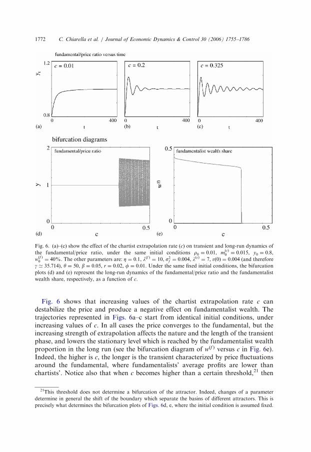
Fig. 6. (a)–(c) show the effect of the chartist extrapolation rate (c) on transient and long-run dynamics of

the fundamental/price ratio, under the same initial conditions r0 ¼ 0:01, mðcÞ0 ¼ 0:015, y0 ¼ 0:8,

wðf Þ0 ¼ 40%. The other parameters are: Z ¼ 0:1, lðf Þ ¼ 10, s2f ¼ 0:004, lðcÞ ¼ 7, vð0Þ ¼ 0:004 (and therefore

g ’ 35:714), y ¼ 50, b ¼ 0:05, r ¼ 0:02, f ¼ 0:01. Under the same fixed initial conditions, the bifurcation

plots (d) and (e) represent the long-run dynamics of the fundamental/price ratio and the fundamentalist

wealth share, respectively, as a function of c.


Fig. 6 shows that increasing values of the chartist extrapolation rate c candestabilize the price and produce a negative effect on fundamentalist wealth. Thetrajectories represented in Figs. 6a–c start from identical initial conditions, underincreasing values of c. In all cases the price converges to the fundamental, but theincreasing strength of extrapolation affects the nature and the length of the transientphase, and lowers the stationary level which is reached by the fundamentalist wealthproportion in the long run (see the bifurcation diagram of wðf Þ versus c in Fig. 6e).Indeed, the higher is c, the longer is the transient characterized by price fluctuationsaround the fundamental, where fundamentalists’ average profits are lower thanchartists’. Notice also that when c becomes higher than a certain threshold,21 then

21This threshold does not determine a bifurcation of the attractor. Indeed, changes of a parameter

determine in general the shift of the boundary which separate the basins of different attractors. This is

precisely what determines the bifurcation plots of Figs. 6d, e, where the initial condition is assumed fixed.

ARTICLE IN PRESS


the system is completely destabilized and no longer converges to the fundamentalprice but ends up in a limit cycle, with zero long-run fundamentalist wealth share andthe market dominated by chartists (see the bifurcation diagrams of y and wðf Þ versusc in Fig. 6d and e, respectively).

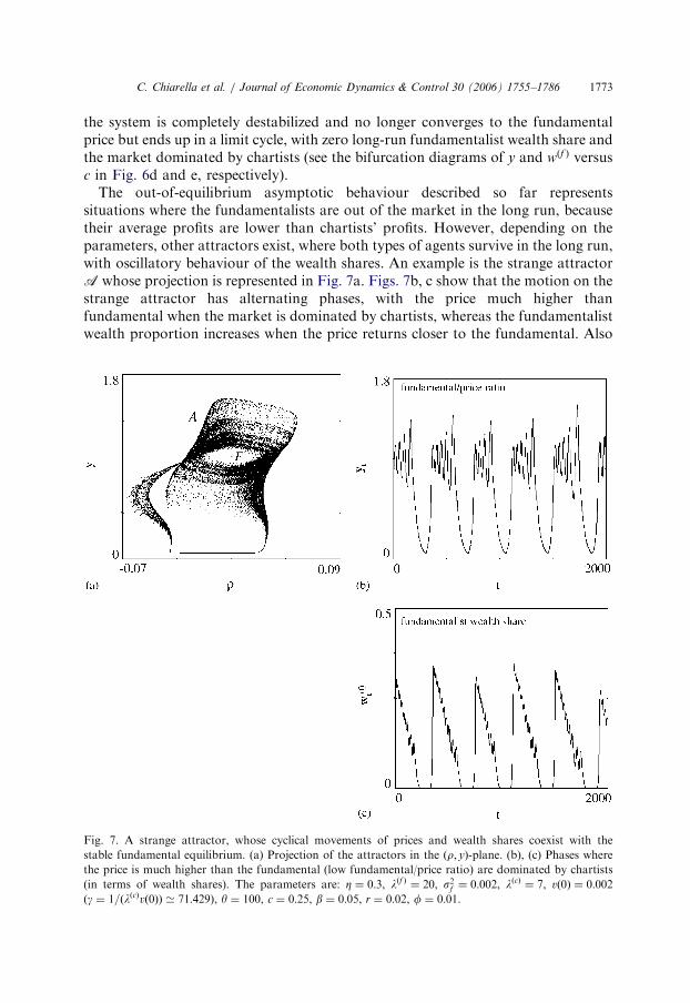
The out-of-equilibrium asymptotic behaviour described so far representssituations where the fundamentalists are out of the market in the long run, becausetheir average profits are lower than chartists’ profits. However, depending on theparameters, other attractors exist, where both types of agents survive in the long run,with oscillatory behaviour of the wealth shares. An example is the strange attractorA whose projection is represented in Fig. 7a. Figs. 7b, c show that the motion on thestrange attractor has alternating phases, with the price much higher thanfundamental when the market is dominated by chartists, whereas the fundamentalistwealth proportion increases when the price returns closer to the fundamental. Also

Fig. 7. A strange attractor, whose cyclical movements of prices and wealth shares coexist with the

stable fundamental equilibrium. (a) Projection of the attractors in the ðr; yÞ-plane. (b), (c) Phases wherethe price is much higher than the fundamental (low fundamental/price ratio) are dominated by chartists

(in terms of wealth shares). The parameters are: Z ¼ 0:3, lðf Þ ¼ 20, s2f ¼ 0:002, lðcÞ ¼ 7, vð0Þ ¼ 0:002ðg ¼ 1=ðlðcÞvð0ÞÞ ’ 71:429Þ, y ¼ 100, c ¼ 0:25, b ¼ 0:05, r ¼ 0:02, f ¼ 0:01.

ARTICLE IN PRESS


in this case the attractor coexists with attracting fundamental steady states, as onecan check by trying different initial conditions, and the role played by the initialwealth share w

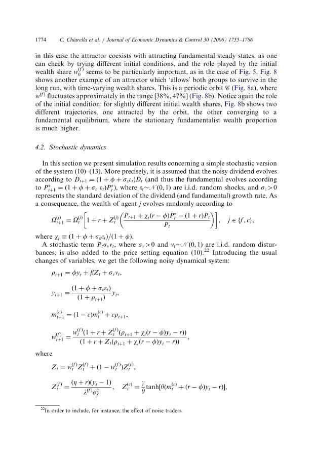
ðf Þ0 seems to be particularly important, as in the case of Fig. 5. Fig. 8

shows another example of an attractor which ‘allows’ both groups to survive in thelong run, with time-varying wealth shares. This is a periodic orbit C (Fig. 8a), wherewðf Þ fluctuates approximately in the range ½38%; 47%� (Fig. 8b). Notice again the roleof the initial condition: for slightly different initial wealth shares, Fig. 8b shows twodifferent trajectories, one attracted by the orbit, the other converging to afundamental equilibrium, where the stationary fundamentalist wealth proportionis much higher.

4.2. Stochastic dynamics

In this section we present simulation results concerning a simple stochastic versionof the system (10)–(13). More precisely, it is assumed that the noisy dividend evolvesaccording to Dtþ1 ¼ ð1þ fþ s��tÞDt (and thus the fundamental evolves accordingto P�tþ1 ¼ ð1þ fþ s� �tÞP

�t ), where �tNð0; 1Þ are i.i.d. random shocks, and s�40

represents the standard deviation of the dividend (and fundamental) growth rate. Asa consequence, the wealth of agent j evolves randomly according to


Ptþ1 þ wtðr� fÞP�t � ð1þ rÞPt

Pt

� �� ; j 2 ff ; cg,

where wt � ð1þ fþ s��tÞ=ð1þ fÞ.A stochastic term Ptsnnt, where sn40 and ntNð0; 1Þ are i.i.d. random distur-

bances, is also added to the price setting equation (10).22 Introducing the usualchanges of variables, we get the following noisy dynamical system:

rtþ1 ¼ fyt þ bZt þ snnt,

ytþ1 ¼ð1þ fþ s��tÞð1þ rtþ1Þ

yt,


ðcÞt þ crtþ1,

wðf Þtþ1 ¼

wðf Þt ð1þ rþ Z

ðf Þt ðrtþ1 þ wtðr� fÞyt � rÞÞ

ð1þ rþ Ztðrtþ1 þ wtðr� fÞyt � rÞÞ,

where

Zt ¼ wðf Þt Z

ðf Þt þ ð1� w

ðf Þt ÞZ

ðcÞt ,

Zðf Þt ¼ðZþ rÞðyt � 1Þ

lðf Þs2f; Z

ðcÞt ¼

gytanh½yðmðcÞt þ ðr� fÞyt � rÞ�,

22In order to include, for instance, the effect of noise traders.

ARTICLE IN PRESS

Fig. 8. An attracting periodic orbit coexists with the stable fundamental equilibrium. (a) Projection of the

two attractors in the ðr; yÞ-plane. (b) The trajectory generated by the initial conditions r0 ¼ mðcÞ0 ¼ 0:01,

y0 ¼ 0:85, wðf Þ0 ¼ 40% converges to the fundamental steady state after a very long transient. If the initial

wealth share wðf Þ0 is decreased to 38%, the system converges to the periodic orbit, with long-run

fluctuations in wealth shares. Here the parameter set is characterized by strong fundamentalist reaction

ðZ ¼ 0:8Þ and strong chartist extrapolation (c ¼ 0:8). The other parameters are: lðf Þ ¼ 10, s2f ¼ 0:004,lðcÞ ¼ 2:5, vð0Þ ¼ 0:004 ðg ¼ 100Þ, y ¼ 50, b ¼ 0:1, r ¼ 0:02, f ¼ 0:01.


and where �t and nt are i.i.d. processes, �tNð0; 1Þ, ntNð0; 1Þ, s�, sn40, andwt ¼ ð1þ fþ s��tÞ=ð1þ fÞ.

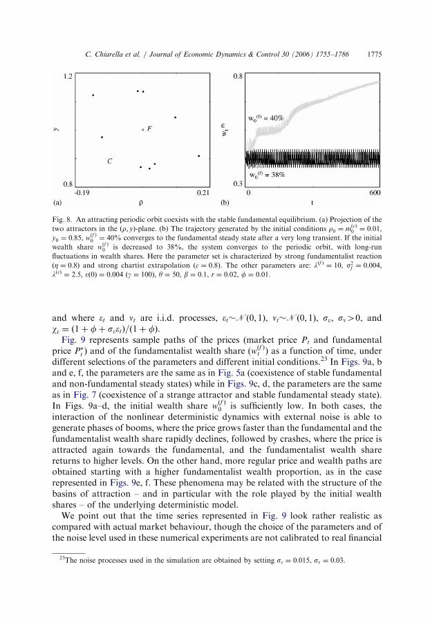
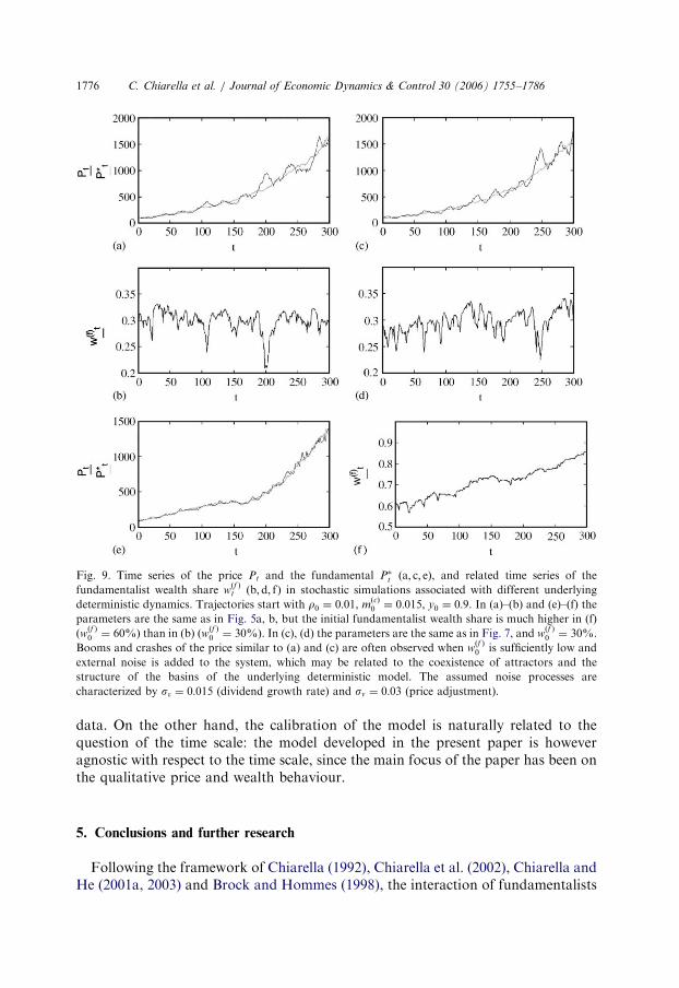
Fig. 9 represents sample paths of the prices (market price Pt and fundamentalprice P�t ) and of the fundamentalist wealth share (w

ðf Þt ) as a function of time, under

different selections of the parameters and different initial conditions.23 In Figs. 9a, band e, f, the parameters are the same as in Fig. 5a (coexistence of stable fundamentaland non-fundamental steady states) while in Figs. 9c, d, the parameters are the sameas in Fig. 7 (coexistence of a strange attractor and stable fundamental steady state).In Figs. 9a–d, the initial wealth share w

ðf Þ0 is sufficiently low. In both cases, the

interaction of the nonlinear deterministic dynamics with external noise is able togenerate phases of booms, where the price grows faster than the fundamental and thefundamentalist wealth share rapidly declines, followed by crashes, where the price isattracted again towards the fundamental, and the fundamentalist wealth sharereturns to higher levels. On the other hand, more regular price and wealth paths areobtained starting with a higher fundamentalist wealth proportion, as in the caserepresented in Figs. 9e, f. These phenomena may be related with the structure of thebasins of attraction – and in particular with the role played by the initial wealthshares – of the underlying deterministic model.

We point out that the time series represented in Fig. 9 look rather realistic ascompared with actual market behaviour, though the choice of the parameters and ofthe noise level used in these numerical experiments are not calibrated to real financial

23The noise processes used in the simulation are obtained by setting s� ¼ 0:015, sn ¼ 0:03.

ARTICLE IN PRESS

Fig. 9. Time series of the price Pt and the fundamental P�t ða; c; eÞ, and related time series of the

fundamentalist wealth share wðf Þt ðb; d; fÞ in stochastic simulations associated with different underlying

deterministic dynamics. Trajectories start with r0 ¼ 0:01, mðcÞ0 ¼ 0:015, y0 ¼ 0:9. In (a)–(b) and (e)–(f) the

parameters are the same as in Fig. 5a, b, but the initial fundamentalist wealth share is much higher in (f)

ðwðf Þ0 ¼ 60%Þ than in (b) ðw

ðf Þ0 ¼ 30%Þ. In (c), (d) the parameters are the same as in Fig. 7, and w

ðf Þ0 ¼ 30%.

Booms and crashes of the price similar to (a) and (c) are often observed when wðf Þ0 is sufficiently low and

external noise is added to the system, which may be related to the coexistence of attractors and the

structure of the basins of the underlying deterministic model. The assumed noise processes are

characterized by s� ¼ 0:015 (dividend growth rate) and sn ¼ 0:03 (price adjustment).


data. On the other hand, the calibration of the model is naturally related to thequestion of the time scale: the model developed in the present paper is howeveragnostic with respect to the time scale, since the main focus of the paper has been onthe qualitative price and wealth behaviour.

5. Conclusions and further research

Following the framework of Chiarella (1992), Chiarella et al. (2002), Chiarella andHe (2001a, 2003) and Brock and Hommes (1998), the interaction of fundamentalists

ARTICLE IN PRESS


and chartists has been incorporated in a market maker model of asset price andwealth dynamics. The resulting dynamical system for asset price and wealth turnsout to be non-stationary, and a stationary system is developed by expressing the lawsof motion in terms of capital gain, fundamental/price ratio and wealth proportionsof the two types of agents. It is found that the presence of fundamentalists andchartists leads the stationary model to have two kinds of steady states, which oftencoexist in the phase space, with different long-run stationary returns and wealthdistributions: fundamental steady states, where the price is at the fundamental level,and non-fundamental steady states, where price grows faster than fundamental, whilethe fundamentalist wealth proportion becomes negligible in the long run.

The chartists’ extrapolation parameter c, together with the chartists’ risk aversionlðcÞ (inversely related to the slope g of their demand function) and the marketreaction coefficient b, play an important role in the local asymptotic stability of thefundamental steady states, and for sufficiently high values of c, b, g the price andreturn dynamics become unstable due to a Neimark – Sacker bifurcation.

The main impression gained from the numerical simulation of the global dynamics(Section 4) is that the model is able to generate a wide range of different dynamicscenarios, with a strong dependence on small changes of the parameters and of theinitial conditions: limit cycles, periodic orbits, strange attractors, cases of coexistence ofmultiple steady states, or coexistence of a steady state with a cyclical attractor. Inparticular, in the case of coexistence of fundamental and non-fundamental steady states,the initial wealth distribution plays a crucial role in determining the long-run evolution.

Another important feature of this model is that it considers explicitly theinterdependence between the price dynamics and the evolution of the wealthdistribution among agent types: it is found that in general fundamentalists’ averageprofits are lower than chartists’ profits (and thus the fundamentalist wealthproportion tends to vanish) when the system moves on a limit cycle or is at a non-fundamental steady state; on the other hand both types of agents survive in the longrun when the market is at a fundamental equilibrium, or when it fluctuates onperiodic orbits or strange attractors. Anyway, in general the fundamentalists do notaccumulate more wealth than the chartists.

We have also considered a stochastic version of the model, simulations of whichhave shown how the coexistence of fundamental and non-fundamental equilibria, aswell as the existence of cyclical attractors, can provide a basis for the onset of boomsand crashes when random disturbances are added to the deterministic model. Wehave also observed that, because of this switching back and forth between thefundamental and non-fundamental equilibria, both groups seem to continue tosurvive with positive wealth shares. Thus, at least in the simple framework of thispaper we can see that supposed ‘irrational’ traders (our chartists) can indeed survivein the long run. Debate on this point in the economics and finance literature goesback at least to Friedman (1953) and Fama (1965).

Our analysis in this paper is based on a simplified model, and some extensions areneeded in order to develop a more realistic one. First, the analysis here has focusedmainly on a deterministic dynamic model which can be interpreted as thedeterministic skeleton of a stochastic model with a noisy dividend process: our

ARTICLE IN PRESS


analysis of a stochastic version of the model could still be regarded as verypreliminary, it would be interesting to analyze in greater detail the interaction of anoisy dividend process with the underlying deterministic scenarios. Second, althoughthe dynamic modelling of the wealth proportions ‘keeps track’ of realized profits ofthe two types of agents and determines endogenously time-varying ‘weights’ offundamentalists and chartists, this model is one with fixed agents’ proportions, in thesense that agents do not switch amongst different strategies on the basis on theirrealized profits or wealth (according to the adaptive belief system introduced byBrock and Hommes, 1997a, 1998). The introduction of ‘switching’ mechanisms andtime-varying proportions (similar to Chiarella and He, 2002) would be an importantextension of this model. Third, the introduction of a more flexible and realistic pricesetting rule, where the market maker inventory position is also taken into account, islikely to lead to more realistic dynamics of returns and wealth fractions.

Acknowledgements

This work has been performed with the financial support of MIUR, Italy, withinthe scope of the national research project ‘‘Nonlinear Models in Economics andFinance: Complex Dynamics, Disequilibrium, Strategic Interaction’’. Chiarellaacknowledges support from ARC Discovery Grant DP 0450526: ‘‘A New Paradigmof Financial Market Behaviour’’. Earlier versions of this paper were presented at the11th Annual Symposium of the Society for Nonlinear Dynamics and Econometrics,Firenze, 13–15 March 2003, and at the 8th Viennese Workshop on Optimal Control,Dynamic Games and Nonlinear Dynamics, Vienna, 14–16 May 2003: we are gratefulto the participants, in particular to Cars Hommes, for stimulating discussions. Wealso would like to thank the organizers and participants of the conference CEF 2004,Amsterdam, and three anonymous referees, whose helpful comments and sugges-tions on an earlier draft have led to major improvements. The usual caveat applies.

Appendix A. The dynamic model under positive supply of shares

In this appendix, we show how the model can be extended to the case of positivenet supply of shares. Similarly to Brock and Hommes (1998), we first derive abenchmark notion of ‘fundamental solution’, which refers to the long-run marketclearing price path that would be obtained if agents were homogeneous with regardto their expectation of the excess return. Furthermore, this price is assumed to satisfythe ‘no-bubbles’ condition.

Denote by NDt ¼ ðO

ðf Þt Z


ðcÞt Þ=Pt the demand (number of shares) and by

NSt the supply of shares at t. The market clearing condition at time t, ND

t ¼ NSt , can

be rewritten as

Xj2ff ;cg

OðjÞt

EðjÞt ½Ptþ1 þDtþ1 � ð1þ rÞPt�

lðjÞVarðjÞt ½rtþ1 þ dtþ1 � r�

¼ NSt P2

t . (17)

ARTICLE IN PRESS


Let us assume that agents have constant (not necessarily homogeneous) beliefs about

the variance of the (excess) return, i.e. s2j;t � VarðjÞt ½rtþ1 þ dtþ1 � r� ¼ s2j , j 2 ff ; cg.

Denote by Ot ¼P

j OðjÞt the total wealth and by w

ðjÞt ¼ OðjÞt =Ot the wealth proportion

of group j, with wðcÞt ¼ 1� w

ðf Þt . If all agents were homogeneous with regard to their

expectation of the excess return, then Eq. (17) could be rewritten as

Et½Ptþ1 þDtþ1� ¼ ð1þ rþQtxtÞPt, (18)

where Qt � NSt Pt=Ot is the value of the supply of shares over total agents’ wealth,

while the quantity

xt ¼X

j

wðjÞt

1

lðjÞs2j

!�1¼ w

ðf Þt

1

lðf Þs2fþ ð1� w

ðf Þt Þ

1

lðcÞs2c

" #�1

is a time-varying weighted harmonic mean of the quantities lðjÞs2j , j 2 ff ; cg, that can

be interpreted as an ‘average’ risk perception. Thus, the quantity pt � Qtxt inEq. (18) would represent the risk premium required by the community of traders tohold the risky asset, under the assumed homogeneous beliefs, and r�t � rþQtxt

would be the required expected return, as perceived at time t. Eq. (18) is anexpectational dynamic equation in the price, in which the required risk premium attime t, as one would expect, is a function of average risk attitudes and beliefs about

risk. In the case of zero net supply ðNSt ¼ 0Þ, Eq. (18) reduces to the ‘no-arbitrage’

equation (2), which has been discussed in Section 2.2. Here, we sketch the structureof the model in the case of positive supply, assuming that agents are homogeneouswith regard to risk aversion and beliefs about the variance. Moreover, we make thesimplifying assumption that in a financial market with growing wealth and priceprocesses, the value of the supply is a constant fraction Q of total wealth,

Qt � NSt Pt=Ot ¼ Q, 8t. A more general case, with heterogeneous risk beliefs and

attitudes, sketched in Chiarella et al. (2004), is left to future research.Let us derive the reference notion of fundamental solution. Denote by l and by s2

the common risk aversion and belief about the variance of the excess return,respectively. Then the (constant) required risk premium pt ¼ p and the requiredexpected return r�t ¼ r� turn out to be p ¼ Qls2, r� ¼ rþ p ¼ rþQls2, and themarket clearing condition (17) yields Et½Ptþ1 þDtþ1� ¼ ð1þ r�ÞPt. Assuminghomogeneous beliefs about expected dividends and a dividend process whichevolves according to Et½Dtþk� ¼ ð1þ fÞkDt, k ¼ 1; 2; . . . ; fX0, the unique funda-mental solution P�t is given by

P�t ¼ð1þ fÞDt

ðr� � fÞ¼ð1þ fÞDt

ðrþQls2 � fÞ, (19)

where P�t evolves over time according to Et½P�tþ1� ¼ ð1þ fÞP�t . The expected

dividend yield and capital gain along the fundamental solution are given byEt½dtþ1� ¼ r� � f, Et½rtþ1� ¼ f, while the expected return is r� ¼ rþQls2 ¼Et½rtþ1� þ Et½dtþ1�.

ARTICLE IN PRESS


Next, by introducing heterogeneous and time-varying beliefs, and followingsimilar steps as in the case of zero supply, we obtain the dynamical system

Ptþ1 ¼ Pt þ fP�t þ PtbðZt �QÞ,


ðcÞt þ c½ðPtþ1 � PtÞ=Pt�,

P�tþ1 ¼ ð1þ fÞP�t ,



Pt

� �� ; j 2 ff ; cg,

where

Ot ¼ Oðf Þt þ OðcÞt ; Zt ¼ ðOðf Þt Z


ðcÞt Þ=Ot,

Zðf Þt ¼

ZðP�t � PtÞ þ fP�t þ ð1þ fÞDt � rPt

Ptls2; Z

ðcÞt ¼

mðcÞt þ ð1þ fÞDt=Pt � r

ls2c;t

and the chartist variance belief s2c;t is assumed in general to be state dependent, withstationary level s2c;t ¼ s2ð¼ s2f Þ at the ‘fundamental solution’. Notice that from (19)we get ð1þ fÞDt ¼ ðr

� � fÞP�t , so that agents’ demand functions can be rewritten as(recall also that ðr� � rÞ ¼ Qls2)

Zðf Þt ¼ðZþ rÞðP�t � PtÞ=Pt þ ðr

� � rÞP�t =Pt

ls2¼ðZþ rÞðP�t � PtÞ=Pt

ls2þQ

P�tPt

,

ZðcÞt ¼

mðcÞt þ ðr

� � fÞP�t =Pt � r

ls2c;t¼

mðcÞt þ ðr� fÞP�t =Pt � r

ls2c;tþ

Qs2

s2c;t

P�tPt

.

A stationary system can be obtained through the same changes of variables used inthe simplified zero-supply case, and similar results about the steady states hold.Notice that at the fundamental steady states (where yt ¼ P�t =Pt ¼ 1, m

ðcÞt ¼ f, and

where s2c;t ¼ s2f ¼ s2 under our assumptions) the total agents’ demand is exactlyequal to the supply, Z

ðcÞ¼ Z

ðf Þ¼ Z ¼ Q ¼ ðr� � rÞ=ls2.

Appendix B. Analysis of the steady states

In this appendix, we derive the steady states of the model, and discuss the stabilityproperties of the fundamental steady state.

B.1. Derivation of the steady states

First of all, notice that the subsets of the phase space of equation wðf Þ ¼ 0 (denoteit by X c) and wðf Þ ¼ 1 (denote it by X f ) are trapping, in the sense that TðX cÞ � X c

ARTICLE IN PRESS


and TðX f Þ � X f , where T is the map (15); these trapping subsets represent the caseswhere only chartists or only fundamentalists survive in the market, respectively.

The steady states of the system are the fixed points ðr; y;mðcÞ;wðf ÞÞ of the map T,obtained by setting ðr0; y0;mðcÞ0;wðf Þ0Þ ¼ ðr; y;mðcÞ;wðf ÞÞ ¼ ðr; y;mðcÞ;wðf ÞÞ in (15).Thus, the steady states must satisfy the following set of conditions:

r ¼ fyþ bZ, (20)

y ¼ yð1þ fÞ=ð1þ rÞ, (21)

mðcÞ ¼ ð1� cÞmðcÞ þ cr, (22)

wðf Þ ¼ wðf Þ1þ rþ Zðf Þðrþ ðr� fÞy� rÞ

1þ rþ Zðrþ ðr� fÞy� rÞ, (23)

where Z ¼ wðf ÞZðf Þ þ ð1� wðf ÞÞZðcÞ, and

Zðf Þ ¼ðZþ rÞðy� 1Þ

lðf Þs2f; ZðcÞ ¼

gytanh½yðmðcÞ þ ðr� fÞy� rÞ�.

Notice first that (22) implies mðcÞ ¼ r. In the following, we consider three separatecases, wðf Þ ¼ 0, wðf Þ ¼ 1, and 0owðf Þo1.

(i) We first consider the case wðf Þ ¼ 0, i.e. we look for the fixed points of therestriction of the map T to the subset X c. Therefore, we neglect Eq. (23) and we setZ ¼ Z

ðcÞin (20). Assume first y40. Then (21) implies r ¼ fð¼ mðcÞÞ, and (20)

becomes

fðy� 1Þ þ bgytanh½yðr� fÞðy� 1Þ� ¼ 0. (24)

Since ðr� fÞ is positive, it follows that the terms fðy� 1Þ and ðbg=yÞ tanh½yðr�fÞðy� 1Þ� are both positive for y41, both negative for yo1, and therefore condition(24) yields y ¼ 1. We denote by ‘fundamental’ steady state the one characterized byy ¼ 1, r ¼ mðcÞ ¼ f.

Now assume y ¼ 0. In this case (20) becomes

rb¼

gytanh½yðr� rÞ�. (25)

Since g1ðrÞ � r=b is a straight line through the origin with positive slope 1=b, andg2ðrÞ � ðg=yÞ tanh½yðr� rÞ� is a strictly increasing S-shaped function, taking valuesin ð�g=y; g=yÞ and vanishing for r ¼ r, it follows that a negative solution of (25)always exists, while (25) admits one or two further positive solutions provided that gor b are sufficiently high (i.e. for low chartist risk aversion or strong price reaction).Moreover, if a positive solution r exists, it necessarily follows that r4r, andtherefore r4f. We denote by ‘non-fundamental’ steady states the ones character-ized by y ¼ 0, r ¼ mðcÞ4f, where r is a positive solution of (25).

(ii) Let us now consider the case wðf Þ ¼ 1, i.e. look for the fixed points of therestriction of the map T to the subset X f . Following similar steps as in the previous

ARTICLE IN PRESS


case, one easily finds that two steady states exist, a fundamental steady state withy ¼ 1, r ¼ f, and a further steady state y ¼ 0, r ¼ �bðZþ rÞ=ðlðf Þs2f Þo0.

(iii) We now consider the case 0owðf Þo1, i.e. we look for fixed pointscharacterized by strictly positive stationary wealth shares of fundamentalists andchartists. Assume first y40. Then (21) implies r ¼ mðcÞ ¼ f, and (20) becomes

fþ bwðf ÞZþ r

lðf Þs2f

!ðy� 1Þ þ bð1� wðf ÞÞ

gytanh½yðr� fÞðy� 1Þ� ¼ 0, (26)

which yields y ¼ 1. Therefore, Zðf Þ ¼ ZðcÞ ¼ Z ¼ 0 and (23) is identically satisfied forany wðf Þ, 0owðf Þo1. Thus, a continuum of fundamental steady states exist.

Assume now y ¼ 0. One can show that in general no fixed points of (15) exist withy ¼ 0, 0owðf Þo1. In fact from (23) such a fixed point would imply

Zðf Þðr� rÞ ¼ ZðcÞðr� rÞ, (27)

where Zðf Þ ¼ �ðZþ rÞ=ðlðf Þs2f Þ, ZðcÞ ¼ ðg=yÞ tanh½yðr� rÞ�. On the other hand, (20)would become

rb¼ wðf ÞZðf Þ þ ð1� wðf ÞÞZðcÞ. (28)

Eq. (28) implies rar (otherwise the left-hand side and the right-hand side of (28)would have opposite sign) and therefore (27) implies Zðf Þ ¼ ZðcÞ, i.e.

�Zþ r

lðf Þs2f¼

gytanh½yðr� rÞ�, (29)

while (28) becomes

rb¼ ZðcÞ ¼

gytanh½yðr� rÞ�,

which has been discussed in the previous case (i) and which in general will not becompatible with (29).

To summarize, if we restrict our analysis to the steady states which arecharacterized by rX0,24 we can identify two types of steady states:

(a)

24

outs

para

‘Fundamental’ steady states, characterized by y ¼ 1, r ¼ mðcÞ ¼ f, any

wðf Þ 2 ½0; 1�, and Zðf Þ¼ Z

ðcÞ¼ Z ¼ 0, i.e. by the price being at the fundamental

and growing at the fundamental rate, any long-run wealth distribution, and zeroexcess demand. As already remarked, these represent a continuum of steadystates.

(b)
‘Non-fundamental’ steady states, characterized by y ¼ 0, wðf Þ ¼ 0, r ¼ mðcÞ4r4f, where r solves r=b ¼ ðg=yÞ tanh½yðr� rÞ�, and Z ¼ Z
ðcÞ¼ ðg=yÞ tanh½yðr�

Though the existence of steady states with ro0 has been proven analytically, they are in general

ide the economically meaningful range of values of r (i.e. r4� 1) for reasonable values of the

meters, and numerical evidence confirms that they are not attracting.

ARTICLE IN PRESS


rÞ�4 0, i.e. by the price growing faster than the fundamental, the fundamental/price ratio approaching zero, market dominated by chartists, and permanentpositive excess demand.

B.2. Local stability conditions of the fundamental steady states

In order to gain some insights about the conditions of local asymptotic stability ofthe ‘fundamental steady states’, and their dependence on the key parameters of themodel, we restrict our analysis to the particular cases where only fundamentalists oronly chartists populate the market, i.e. the cases in which the dynamical system isrestricted to the subspace X f (wðf Þ ¼ 1) or X c (wðf Þ ¼ 0), respectively. The analysis ofthe local stability at the continuum of steady states with 0owðf Þo1 would becomemuch more difficult to work out, given the higher dimension of the dynamical systemin this case and the dependence of the Jacobian on the stationary wealth level wðf Þ.On the other hand, the analysis of the extreme cases is quite illuminating about therole played by the key parameters in stabilizing or destabilizing the steady state, andnumerical simulations confirm that the sensitivity to the parameters in the generalcase is similar to what emerges from the particular cases wðf Þ ¼ 1 and wðf Þ ¼ 0.

(a) The map T ðf Þ : ðr; yÞ7�!ðr0; y0Þ which drives the dynamical system restricted toX f is

T ðf Þ :r0 ¼ fyþ bZðf Þ;


(

where Zðf Þ ¼ ðZþ rÞðy� 1Þ=ðlðf Þs2f Þ and the dynamic equation for mðcÞ has beenneglected given that it has no influence on the dynamics of r and y. The map T ðf Þ canindeed be reduced to the one-dimensional map with equation y0 ¼ F ðyÞ, where

F ðyÞ ¼ yð1þ fÞ 1þ fyþ bðZþ rÞðy� 1Þ

lðf Þs2f

" #�1.

Given that y ¼ 1 at the fundamental steady state, one easily finds

dF ðyÞ

dy

��y¼1

¼1� bðZþ rÞ=ðlðf Þs2f Þ

ð1þ fÞo1.

Thus, the local asymptotic stability condition �1odF ðyÞ=dyjy¼1o1 reduces tobðZþ rÞ=ðlðf Þs2f Þo2þ f. Moreover, for bðZþ rÞ=ðlðf Þs2f Þ ¼ 2þ f the stable steadystate becomes unstable through a Flip-bifurcation.

(b) The map T ðcÞ : ðr; y;mðcÞÞ7�!ðr0; y0;mðcÞ0Þ which governs the dynamical systemrestricted to X c is

T ðcÞ :

r0 ¼ fyþ bZðcÞ;


mðcÞ0 ¼ ð1� cÞmðcÞ þ cr0;

8><>:

ARTICLE IN PRESS


where ZðcÞ ¼ ðg=yÞ tanh½yðmðcÞ þ ðr� fÞy� rÞ�. This map could in fact be immedi-ately reduced to a two-dimensional map, since r0 is a function of y, mðcÞ, but one caneasily handle the three-dimensional specification as well. The Jacobian matrix of T ðcÞ,evaluated at the fundamental steady state F (where r ¼ mðcÞ ¼ f, y ¼ 1) is given by

DT ðcÞðF Þ ¼

0 fþ bgðr� fÞ bg

0 ½1� bgðr� fÞ�=ð1þ fÞ �bg=ð1þ fÞ

0 c½fþ bgðr� fÞ� ð1� cÞ þ cbg

264

375,

which implies that one eigenvalue is 0 (and thus smaller than one in modulus), whilethe remaining two eigenvalues are the ones of the lower-right two-dimensional blockof DT ðcÞðF Þ (denote it by A). Let

TrðAÞ ¼ 1�fþ bgðr� fÞ

1þ fþ ð1� cÞ þ cbg,

DetðAÞ ¼ ð1� cÞ 1�fþ bgðr� fÞ

1þ f

� �þ cbg

be the trace and the determinant of A, respectively. The characteristic polynomial ofA is given by PðzÞ ¼ z2 � TrðAÞzþDetðAÞ. A well known necessary and sufficientcondition (see e.g. Gumowski and Mira, 1980; Medio and Lines, 2001) for botheigenvalues of A to be smaller than one in modulus, which implies a locally attractingsteady state, is

Pð1Þ ¼ 1� TrðAÞ þDetðAÞ40;

Pð�1Þ ¼ 1þ TrðAÞ þDetðAÞ40;

Pð0Þ ¼ DetðAÞo1:

8><>: (30)

In terms of the parameters of the model (r, f, c, and the aggregate parameter bg) theset of inequalities (30) can be rewritten as

c½fþ bgðr� fÞ�40, (31)

bg½ð2� cÞðr� fÞ � 2cð1þ fÞ�oð2� cÞð2þ fÞ, (32)

bg½cð1þ rÞ � ðr� fÞ�oðcþ fÞ. (33)

Condition (31) is always true under our assumptions about the parameters ðr4fÞ.Since 0oco1, the right-hand side of (32) is positive, and this implies that (32) is

satisfied when ½ð2� cÞðr� fÞ � 2cð1þ fÞ�p0, i.e. cX2ðr� fÞ=½ðr� fÞ þ 2ð1þ fÞ�,while in the opposite case, co2ðr� fÞ=½ðr� fÞ þ 2ð1þ fÞ�, condition (32) is satisfiedonly for

bgoð2� cÞð2þ fÞ

2ðr� fÞ � c½ðr� fÞ þ 2ð1þ fÞ�.

Finally, the right-hand side of (33) is positive, and this implies that (33) is satisfiedwhen cpðr� fÞ=ð1þ rÞ, while in the opposite case c4ðr� fÞ=ð1þ rÞ condition (33)

ARTICLE IN PRESS


is satisfied only for

bgoðcþ fÞ

cð1þ rÞ � ðr� fÞ.

Taking r, f as given, the region of local asymptotic stability and the bifurcationcurves can be represented in the space of the parameters ðc;DÞ, where D � bg,25 asqualitatively shown in Fig. 2 (shaded area). In particular, when D or c are varied sothat the bifurcation curve of equation D ¼ DNSðcÞ ¼ ðcþ fÞ=½cð1þ rÞ � ðr� fÞ� iscrossed from inside the stability region (as shown in Fig. 2), then a supercritical26

Neimark – Sacker bifurcation occurs, which is followed by the appearance of a stable

limit cycle.The stability region of Fig. 2 shows that for D low enough ðDp1=ð1þ rÞÞ the

fundamental steady state F is stable for any value of the chartist extrapolationparameter c, 0oco1, while in general a Neimark – Sacker bifurcation will occurwhen D41=ð1þ rÞ and c is increased above a certain threshold.27

References

Beja, A., Goldman, M.B., 1980. On the dynamic behavior of prices in disequilibrium. Journal of Finance

35, 235–248.

Brock, W., Hommes, C.H., 1997a. A rational route to randomness. Econometrica 65 (5), 1059–1095.

Brock, W., Hommes, C.H., 1997b. Models of complexity in economics and finance. In: Heij, C.,

Schumacher, J.M., Hanzon, B., Praagman, C. (Eds.), System Dynamics in Economic and Financial

Models. Wiley, New York, pp. 3–41.

Brock, W., Hommes, C.H., 1998. Heterogeneous beliefs and routes to chaos in a simple asset pricing

model. Journal of Economic Dynamics and Control 22, 1235–1274.

Brock, W., LeBaron, B., 1996. A structural model for stock return volatility and trading volume. Review

of Economics and Statistics 78, 94–110.

Campbell, J.Y., Viceira, L.M., 2002. Strategic Asset Allocation: Portfolio Choice for Long-term Investors.

In: , Clarendon Lectures in Economics. Oxford University Press, Oxford.

Chen, S.-H., Yeh, C.-H., 2002. On the emergent properties of artificial stock markets: the efficient market

hypothesis and the rational expectations hypothesis. Journal of Economic Behavior and Organization

49, 217–239.

Chiarella, C., 1992. The dynamics of speculative behaviour. Annals of Operations Research 37, 101–123.

Chiarella, C., He, X., 2001a. Heterogeneous beliefs, risk and learning in a simple asset pricing model.

Computational Economics 19 (1), 95–132.

Chiarella, C., He, X., 2001b. Asset price and wealth dynamics under heterogeneous expectations.

Quantitative Finance 1 (5), 509–526.

Chiarella, C., He, X., 2002. An adaptive model on asset pricing and wealth dynamics with heterogeneous

trading strategies. Working Paper no. 84, School of Finance and Economics, UTS.

25The aggregate parameter D � bg is the partial derivative of r0 with respect to mðcÞ (evaluated at the

steady state F) and can be interpreted as the sensitivity of tomorrow’s return with respect to today’s

chartist expected return.26We have numerical evidence of the supercritical nature of the Neimark – Sacker bifurcation.27The branch of the Flip boundary qualitatively represented in Fig. 2 is of no practical interest in this

case, because it is related to very low values of c ð0oco2ðr� fÞ=½ðr� fÞ þ 2ð1þ fÞ� ’ 0:009852 in our

numerical examples).

ARTICLE IN PRESS


Chiarella, C., He, X., 2003. Heterogeneous beliefs, risk and learning in a simple asset pricing model with a

market maker. Macroeconomic Dynamics 7 (4), 503–536.

Chiarella, C., Dieci, R., Gardini, L., 2002. Speculative behaviour and complex asset price dynamics: a

global analysis. Journal of Economic Behavior and Organization 49, 173–197.

Chiarella, C., Dieci, R., Gardini, L., 2004. Asset price and wealth dynamics in a financial market with

heterogeneous agents. Research Paper no. 134, Quantitative Finance Research Centre, School of

Finance and Economics, University of Technology Sydney.

Day, R.H., Huang, W., 1990. Bulls, bears and market sheep. Journal of Economic Behavior and

Organization 14, 299–329.

Fama, E.F., 1965. The behavior of stock-market prices. Journal of Business 38, 34–105.

Farmer, J., Joshi, S., 2002. The price dynamics of common trading strategies. Journal of Economic

Behavior and Organization 49, 149–171.

Friedman, M., 1953. The case for flexible exchange rates. In: Essays in Positive Economics. University of

Chicago Press, Chicago.

Gaunersdorfer, A., 2000. Endogenous fluctuations in a simple asset pricing model with heterogeneous

agents. Journal of Economic Dynamics and Control 24, 799–831.

Gumowski, I., Mira, C., 1980. Dynamique Chaotique. Cepadues, Toulouse.

Hens, T., Schenk-Hoppe, K.R., 2006. Markets do not select for a liquidity preference as behavior towards

risk. Journal of Economic Dynamics and Control 30, 279–292.

Hommes, C.H., 2002. Modeling the stylized facts in finance through simple nonlinear adaptive systems.

Proceedings of the National Academy of Sciences 99 (3), 7221–7228.

Hommes, C.H., 2006. Heterogeneous agent models in economics and finance. In: Judd, K.L., Tesfatsion,

L. (Eds.), Handbook of Computational Economics, Volume 2: Agent-Based Computational

Economics, Handbooks in Economics 13, North-Holland, Amsterdam.

Hommes, C.H., Huang, H., Wang, D., 2005. A robust rational route to randomness in a simple asset

pricing model. Journal of Economic Dynamics and Control 29, 1043–1072.

Kirman, A., 1991. Epidemics of opinion and speculative bubbles in financial markets. In: Taylor, M. (Ed.),

Money and Financial Markets. Macmillan, London.

LeBaron, B., 2006. Agent-based computational finance. In: Judd, K.L., Tesfatsion, L. (Eds.), Handbook

of Computational Economics, Volume 2: Agent-Based Computational Economics, Handbooks in

Economics 13, North-Holland, Amsterdam.

Levy, M., Levy, H., Solomon, S., 1994. A microscopic model of the stock market. Economic Letters 45,

103–111.

Levy, M., Levy, H., Solomon, S., 1995. Microscopic simulation of the stock market: the effect of

microscopic diversity. Journal de Physique I France 5, 1087–1107.

Levy, M., Levy, H., Solomon, S., 2000. Microscopic Simulation of Financial Markets: From Investor

Behavior to Market Phenomena. Academic Press, New York.

Lux, T., 1998. The socio-economic dynamics of speculative markets: interacting agents, chaos and the fat

tails of return distributions. Journal of Economic Behavior and Organization 33, 143–165.

Madhavan, A., 2000. Market microstructure: a survey. Journal of Financial Markets 3, 205–258.

Madhavan, A., Smidt, S., 1993. An analysis of changes in specialist inventories and quotations. Journal of

Finance 48 (5), 1595–1628.

Medio, A., Lines, M., 2001. Nonlinear Dynamics. Cambridge University Press, Cambridge, UK.

Zeeman, E.C., 1974. On the unstable behaviour of stock exchanges. Journal of Mathematical Economics

1, 39–49.

Documents

Asset price and wealth dynamics in a financial market with heterogeneous agents