Quantitative Macroeconomic Models with

Heterogeneous Agents

Per Krusell∗

Princeton University

Anthony A. Smith, Jr.∗

Yale University

March 2006

∗We would like to thank Torsten Persson for valuable comments, Rafael Lopes de Melo for

research assistance, and the National Science Foundation for financial support.

1 Introduction

The present paper reviews recent research aimed at constructing a theoretical model of

the macroeconomy with five key elements: (i) it is based on rational decision making by

consumers and firms using standard microeconomic theory beginning with assumptions on

preferences and technology; (ii) it is dynamic, so that savings and investment decisions

are determined by intertemporal decisions; (iii) it has stochastic aggregate shocks which

lead to macroeconomic upswings and downswings; (iv) it considers general equilibrium,

so that factor prices and interest rates are endogenous; and (v) it has a heterogeneous

population structure where consumers differ in wealth and face idiosyncratic income shocks

against which they cannot fully insure. As argued by Lucas (1976), the four first elements

seem necessary in any model that aims to evaluate the effects and desirability of economic

policy, and they are by now standard and rather broadly accepted as very important if not

indispensable. What is new in the present work is the fifth element: heterogeneity.

The incorporation of a cross-section of consumers, with an accompanying nontrivial de-

termination of the wealth distribution and of individual wealth transitions, is important

for at least two reasons. First, it constitutes a robustness check on representative-agent

macroeconomic models. Wealth is very unevenly distributed in actual economies. Moreover,

a wide range of applied microeconomic studies suggests that, because of the incompleteness

of insurance markets, wealth aggregation—equal propensities to save, hedge against risk,

and work—fails.1 Indeed, an important goal of the work discussed here is to establish a

solid connection with the applied microeconomic literature studying consumption and labor

supply decisions. So, put differently, the first reason to worry about inequality is that it may

influence the macroeconomy.

Second, there is widespread interest in the determination of inequality per se, and in the

possibility that macroeconomic forces influence inequality. Specifically, business cycles may

affect the rich and the poor differently, and macroeconomic policy may also have impor-

1For surveys, see Attanasio (2005), Blundell and Stoker (2003), and Browning, Hansen, and Heckman(2005).

1

tant distributional implications. If so, they ought to be taken into account in the welfare

evaluation of policy.

The purpose of the present paper is not, however, to answer the two questions above:

we will not provide a detailed assessment of the extent to which inequality influences the

macroeconomy, and neither will we explore in any generality how inequality is determined.

We will, instead, focus on the methodological aspect of these questions. The task of solv-

ing macroeconomic models with nontrivial heterogeneity appears daunting. In short, the

determination of the equilibrium dynamics of the cross-section of wealth requires both solv-

ing dynamic optimization problems with large-dimensional state variables and finding fixed

points in large-dimensional function spaces. Because of the so-called “curse of dimensional-

ity”, computer speed alone cannot suffice as a remedy to the problem of high dimensionality.

Recent progress, however, now permits such analysis to take place. Thus, we will review in

detail how and why the new methods work. In so doing, we will also provide some illustrative

results touching on the two motivating questions.

The illustrations we use allow the reader to obtain insights into how to make this kind of

theory operational. They also constitute examples of two important points. First, for some

issues, the incorporation of inequality does not seem essential. The aggregate behavior of

a model where the only friction—indeed the only reason why exact aggregation would not

apply—is the absence of insurance markets for idiosyncratic risk is almost identical to that of

a representative-agent model. Thus, for purely aggregate issues where this model is deemed

appropriate, one could simply analyze a representative-agent economy: the representative-

agent model is robust.

Second, for other issues and other setups, the representative-agent model is not robust.

Though we do not claim generality, we suspect that the addition of other frictions is key

here. As an illustration we add a certain form of credit-market constraints to the setup

with missing insurance markets. We show here that for asset pricing—in particular, the

determination of the risk-free interest rate—it can make a big difference whether one uses a

representative-agent model or not.

The key insight to solving the model with consumer heterogeneity using numerical meth-

ods is “approximate aggregation” in wealth. Exact aggregation in wealth means that all

2

aggregates, such as prices and aggregate capital, depend only on average capital (or, more

generally, wealth) in the economy. Thus, under aggregation, propensities to undertake dif-

ferent activities (such as saving, portfolio allocations, and working) are equalized among

consumers of all wealth levels, so that redistribution of capital among agents does not in-

fluence totals. Approximate aggregation means that aggregates almost do not depend on

anything but average capital. The implication of approximate aggregation therefore is that

individual decision makers make very small mistakes by ignoring how higher-than-first mo-

ments of the wealth distribution influence future prices.

If, in contrast, aggregation fails, such moments by definition do influence savings, portfolio

decisions, and so on, thus affecting not only the future distribution of wealth, but also average

resources available in the future, and hence also future prices relevant to the agent’s current

decisions. Thus, approximate aggregation allows one to solve the problems of forward-

looking agents with a very small set of state variables—aggregate capital only—and attain

nonetheless a very high degree of accuracy. This is the key insight. The specific numerical

procedure we outline here is the natural one, given this insight, but it does not constitute

the only method that could be used to exploit this insight.

The computational algorithm has two key features. First, it is based on bounded ratio-

nality in the sense that we endow agents with boundedly rational perceptions of how the

aggregate state evolves: they think that no other moments than the first moment of the

wealth distribution matters. Second, we use solution by simulation, which works as follows:

(i) given the boundedly rational perceptions, we solve the individuals’ problems using stan-

dard dynamic-programming methods; (ii) we draw individual and aggregate shocks over time

for a large population of individuals; (iii) we evaluate the decision rules for an initial wealth

distribution and the simulated shocks and, using a method for clearing markets in every

time period along the simulation, we generate a time series for all aggregates; and finally

(iv) we compare the perceptions about the aggregates to those in the actual simulations, and

these perceptions are then updated. We think that this approach—bounded rationality and

solution by simulation—can be a productive also for other applications, and we therefore

devote space to a careful description of it.2

2We note that it has been employed in a variety of other contexts, e.g., Cooley, Marimon, and Quadrini(2004), Cooley and Quadrini (2006), Khan and Thomas (2003, 2005), and Zhang (2005).

3

The present paper consists of two parts. In the first part we outline and show how to

solve the “big model”—the infinite-horizon, stochastic general-equilibrium model with id-

iosyncratic risk and incomplete insurance. For ease of exposition, we focus in this part on

idiosyncratic employment risk. We point out that the baseline model without heterogeneity

in anything but wealth and employment status generates much less wealth inequality than

that seen in the data. Based on this insight, we discuss what kinds of (richer) model frame-

works might generate more wealth dispersion. Moreover, we argue that it is important to

analyze this issue further, because the evaluation of policy aimed at improving the allocation

of risk likely critically depends on what determines the wealth dispersion.

The second part of the paper contains a two-period version of the big model. The two-

period model is useful because it is a convenient laboratory for illustrating, and testing the

robustness of, approximate aggregation. In particular, in the two-period model, one can

solve for an equilibrium with arbitrary precision: because the wealth distribution in the first

period is exogenous we can vary it to trace out how aggregates move.

In contrast, in the infinite-horizon model the wealth distribution evolves in a funda-

mentally endogenous manner, and equilibria are constructed in a guess-and-verify manner:

assuming that individuals perceive only one moment of the wealth distribution to matter,

one proceeds to find a(n almost) fixed point. In this model, it is not clear if this is the

only (approximate) equilibrium or, perhaps more fundamentally, whether the approximate

equilibrium is actually close to an exact equilibrium.

In the two-period model, we can examine such doubts. We find, for the two-period model,

that the equilibrium with approximate aggregation, constructed as for the corresponding

infinite-horizon economy, is indeed very close to the exact (and unique) equilibrium. To our

knowledge, this kind of two-period model has not been analyzed before, and we think it is

a very valuable tool to use for “pilot studies” of more complex economies. We also use the

two-period model to illustrate how aggregate policy can have differing effects on the welfare

of different kinds of consumers. Finally, we look at a version of the 2-period model where

there is another friction—entrepreneurs have to fund their investment projects out of own

funds or borrowed money and cannot sell equity—and demonstrate that the determination of

the risk-free rate is quite different in this model than in its representative-agent counterpart.

4

The organization of the paper may look a little backward. It starts with two sections on

the big model: Section 2 discusses the representative-agent model and Section 3 discusses

the model with partially insurable idiosyncratic risk. Section 4 then discusses the two-period

model. A reverse order—thus starting with the simple setup and adding complication later—

might for some purposes be appropriate, and indeed it is possible to read the paper in such

an order. We begin with the big model for two reasons. First, we find it useful to state the

goal of the work at the outset, which is to analyze the infinite-horizon problem with all its

features. In doing this, we also motivate the work in the sense of explaining the problem that

needs to be overcome—the dynamic determination of a large-dimensional object. Second, the

specific computational method we use in the infinite-horizon model—one based on boundedly

rational perceptions—can be applied in the two-period model. Though the two-period model

does not require this method—it can be solved exactly—using the method in this context

illustrates how our infinite-horizon method works, while at the same time showing that it

works well also in the two-period model. What is less unusual is that our concluding section,

Section 5, comes last.

2 The representative-agent economy

We describe our main framework in this section and in Section 3. It is, in essence, a typical

“real business-cycle” model—aggregate fluctuations have their origin in technology shockd

and there is no money—with consumer heterogeneity and incomplete insurance against id-

iosyncratic unemployment risk.3 In this section we lay out the representative-agent model—

in which consumers can insure fully against idiosyncratic risk—and then in Section 3 we lay

out the heterogeneous-agent model in which consumers cannot.

The representative-agent economy, our baseline setup, has preferences given by

E

[

∞∑

t=0

βtu(ct, 1 − nt)

]

,

where consumption, ct, has to be non-negative and labor, nt, has to be in [0, 1]. The resource

constraint is

ct + kt+1 = F (zt, kt, nt) + (1 − δ)kt + a,

3The reliance on a real model and on technology shocks is mainly chosen for convenience. We suspectthat the key findings are robust to the exact mechanism driving business cycles, though such a robustnesscheck has not been performed.

5

where kt also has to be non-negative. Standard assumptions on primitives, which we will

adopt here, are that β and δ are in [0, 1], that u is strictly concave, increasing in each

argument, and twice continuously differentiable, and that F is strictly increasing in all

arguments, homogenous of degree in one and concave in the second two arguments, and

twice continuously differentiable. Assumptions are also needed on the stochastic process for

zt, but we defer description of this process until later. The nonnegative constant a is a form

of endowment, perhaps interpreted as an exogenous amount of home production.

2.1 Sequential competitive equilibrium

A decentralized equilibrium for this economy can be described as follows. Consumers solve

max{ct,kt+1,nt,bt+1}∞t=0

E

[

∞∑

t=0

βtu(ct, 1 − nt)

]

s.t.

ct + qtbt+1 + kt+1 = bt + (1 + rt − δ)kt + wtnt + a ∀t;

here, we use bt to be the units of riskless bonds held, qt the time-t price of a bond that pays

one unit at time t+1 in all states of nature, and rt and wt the rental rates of capital and labor,

respectively. The consumer takes prices as given when solving this problem. We suppress

the dependence of all variables—prices as well as choice variables—on the uncertainty: in

effect, we are dealing with stochastic processes. Finally, the maximization problem above

presumes another condition, namely a constraint that prevents running Ponzi schemes.

Similarly, firms maximize profits at each date and state, implying that rt = Fk(zt, kt, nt)

and wt = Fn(zt, kt, nt). A sequential competitive equilibrium is a set of stochastic sequences

for all quantities and prices such that (i) the quantities solve the consumer problem; (ii)

quantities and prices satisfy the firm’s first-order conditions stated above; (iii) the resource

constraint is satisfied; and (iv) the bond market clears, i.e., bt equals zero for all t (it is

assumed that b0 = 0).

Note that this economy can be interpreted as one with a continuum of agents with

identical preferences and identical initial wealth where, in equilibrium, since each consumer’s

maximization problem has a unique solution, all consumers choose the same savings, portfolio

allocation, and hours worked.

6

2.2 Recursive competitive equilibrium

To solve dynamic equilibrium models numerically, it is useful to use recursive methods; in

our economy with idiosyncratic risk, these methods are especially helpful if not indispens-

able. Using recursive language involves, first and foremost, expressing behavior and prices as

a function of individual and aggregate state variables. The aggregate state variable here is

(k, z), where by k we now mean aggregate (mean, or total) capital: this is what is predeter-

mined in any given period, and relevant, because it is what determines prices and therefore

any behavior.

A recursive competitive equilibrium for the representative-agent model is defined as func-

tions V , hk, hn, hb, Hk, Hn, R, W , and Q such that

1. V (ω, k, z) solves

V (ω, k, z) = maxk′,n,b′

u(ω + a + nW (k, z) − k′ − Q(k, z)b′)+

E[V (b′ + k′(1 − δ + R(Hk(k, z), z′)), Hk(k, z), z′)|z]

for all (ω, k, z).

2. (hk(ω, k, z), hn(ω, k, z), hb(ω, k, z)) attains the maximum, for all (ω, k, z), in the above

maximization problem.

3. The input pricing functions satisfy, for all (k, z),

R(k, z) = Fk(z, k, Hn(k, z)) and W (k, z) = Fn(z, k, Hn(k, z)).

4. Consistency: for all (k, z),

Hk(k, z) = hk(k(1 − δ + R(k, z)), k, z),

Hn(k, z) = hn(k(1 − δ + R(k, z)), k, z),

and

0 = hb(k(1 − δ + R(k, z)), k, z).

Thus, we use ω to denote individual asset wealth in the beginning of any period, a variable

which in equilibrium must equal k(1− δ + R(k, z)), since bonds are in zero net supply. The

7

consistency conditions simply require that, at the equilibrium value for ω, the individual

behaves as the aggregate behaves, with h representing the individual and H the aggregate.

Notice that (k, z) in the consumer’s problem are not directly influencing the consumer;

if consumers knew current prices and perceived a distribution for future prices, (k, z) would

be superfluous. However, (k, z) determines current prices directly, and by determining the

representative agent’s behavior, it determines the distribution of future prices as well.

Our market structure assumes that there are two assets: capital and bonds. If the

domain for z′ has only two values given any current z, then two assets suffice for completing

markets. What if the domain for uncertainty is larger? A complete-markets structure would

then require more assets, and it is often convenient to introduce, in addition to capital and

bonds, “Arrow securities” or “contingent claims”, which pay 1 unit of consumption in one

of the states next period and 0 otherwise. But it is not necessary to introduce these assets

in a representative-agent economy. Because consumers are identical in this model, each

consumer’s holdings of each of the added contingent claims have to be zero in equilibrium,

just as holdings of bonds have to be zero. Thus, the market structure does not matter in a

representative-agent economy, and for this reason we do not need to include the additional

assets in the equilibrium definition. For the same reason, bonds do not have to be included

either. We include bonds here because doing so offers a convenient parallel with the model

in the next section, where bonds are present and play a nontrivial role.

2.3 Aggregation

Suppose now that we were to permit differences in individual wealth. It is well known

that, if u is in a certain class (e.g., if it equals α log c + (1 − α) log(1 − n)), then there is

aggregation in wealth, presuming that the market structure is complete (for the purpose of

this discussion, suppose that capital and bonds complete the asset markets).4 Aggregation

in wealth means, in terms of the recursive equilibrium definition, that hk(ω, k, z) is linear in

ω (and similarly for hn and hb), i.e., that it can be written hk(ω, k, z) = µ(k, z) + λ(k, z)ω.

The key point is that µ and λ are functions that depend only on k and z, so that the

function hk is linear in individual wealth, i.e., consumers with different wealth levels have

4Here, we have to we presume interior solutions for leisure. For a description of the class of preferencesthat delivers aggregation, see Altug and Labadie (1994).

8

equal marginal propensities to save out of individual wealth. In this case, with heterogeneity

in the distribution of ωs across people, total capital savings and total hours worked do not

depend on anything but the mean of the distribution of ωs, i.e., on k(1 − δ)R(k, z)).

In the economy with idiosyncratic, imperfectly insurable risk decision rules will not be

linear in individual wealth. However, as we shall see, decision rules will be almost linear in

wealth.

2.4 Computation

How is a recursive competitive equilibrium of the representative-agent economy computed

numerically? There are two ways to proceed. One is to solve the planning problem for al-

locations directly, since the equilibrium is Pareto optimal in the absence of frictions. Given

the allocations one would then simply construct R and W using the marginal-product ex-

pressions. For Q, one would just use the first-order condition for bonds from the equilibrium

definition, evaluated using the allocation obtained in the previous step.

The other approach is to only use conditions from the equilibrium definition. If one is

interested in aggregate allocations and prices only (and not in value functions and individual

decision rules), one can also compute the equilibrium easily, without the need to find either

value functions or individual decision rules. This is achieved by first deriving first-order

conditions using the consumer’s dynamic-programming problem and using the envelope con-

dition to eliminate the value-function derivative from these first-order conditions. In those

first-order conditions—one for savings and one for leisure—one then replaces all individual

choice variables with the equilibrium functions, and one replaces the pricing functions R

and W with their marginal-product versions. Thus, one arrives at two functional first-order

conditions: the two equations have to hold for all k and z. The unknowns in the two func-

tional equations are the two functions Hk(k, z) and Hn(k, z). Since the equilibrium, again,

is Pareto optimal, these functional first-order conditions are identical to those implied by

the planning problem. However, the approach of solving the functional first-order conditions

of the representative agent for the equilibrium decision rules works also in the case where

there are taxes or other reasons why the equilibrium is not optimal (e.g., in the presence of

monopolistic competition), in which case the equilibrium cannot be found just by solving a

9

planning problem.

Aa variety of numerical methods can be employed for solving the dynamic-programming

problem, either in its value-function version or its first-order-condition version. We will not

discuss these methods here, since there is an ample literature on this topic.

3 The economy with idiosyncratic unemployment risk

In this section, we incorporate imperfectly insurable unemployment risk into the baseline

model described in Section 2.

3.1 Preliminaries: a steady state without aggregate shocks

We first study the model without aggregate shocks. The classic references here are Bew-

ley (undated) and Aiyagari (1994); Huggett (1997) studies steady states and transitional

dynamics.5

Suppose that ǫ ∈ {ǫℓ, ǫh} denotes the employment status of a particular consumer, with ǫh

and ǫℓ denoting the number of “employed” and “unemployed” labor input units, respectively

(we will mostly assume (ǫℓ, ǫh) = (0, 1)). ǫ is random and statistically independent across

consumers.6 Let the transitions between employment states for an individual be governed

by a two-state Markov chain whose probability transition matrix has typical element πǫ|ǫ.

We assume that ǫ satisfies a law of large numbers: at any point in time, the total fraction

of consumers with ǫ = 1 is known with certainty.

Suppose moreover that there are no other assets in the economy than those mentioned

above, i.e., bonds and capital. Finally, suppose that there are constraints on the agents

ability to borrow, such as separate lower bounds on capital and bonds or a lower bound on

net next-period asset wealth.7 Then the consumer’s budget constraint in period t can be

5For further characterization and comparative statics, see Miao (2002).6A common alternative assumption is that ǫ is individual-specific productivity, which can take on many

more values than two: there is wage risk. We adopt our simpler setup here simply for ease of exposition.7The assumption of exogenously incomplete asset markets of this sort, along with restrictions on borrow-

ing, is made in order to mimic real-world arrangements. Clearly, it would be preferable to make assumptionson a more primitive level so that the market structure would (i) be derived endogenously and (ii) maintainthe key realistic features. Fully satisfactory such setups do not, to our knowledge, yet exist, but Allen (1985)and Cole and Kocherlakota (2001) are promising attempts. For an “in-between” approach, where someinstitutional features are given exogenously but others derived, see Chatterjee et al (2002).

10

written as

ct + qtbt+1 + kt+1 = bt + rtkt + ǫtwtnt + a,

with bt+1 ≥ b and kt+1 ≥ k.8

These individual-level assumptions are the key assumptions on which the model with

idiosyncratic risk rests. The equilibrium is otherwise defined as in the previous sections,

apart from the special attention that needs to be paid to exactly how the distribution of

wealth evolves over time.

To this end, let Γ denote the current measure over wealth and employment status. We

need to define a joint measure, since these two variables will be related in equilibrium:

employment outcomes will influence wealth. So Γ(B, ǫ) reports how many consumers have

ω ∈ B and this value for ǫ, for any interval B and ǫ.

The idea now is that, though for any initial distribution Γ0 there will be a nontrivial

transition path for the distribution of wealth, one can imagine a stationary equilibrium,

or steady state, where Γ has settled down to a time-invariant function. In such a case,

individuals continue to experience shocks over time, but for every interval B and value for ǫ,

Γ(B, ǫ) is constant: people move around within the distribution, but the number of employed

with less than a given amount of wealth is the same in every period. In a steady state, total

assets are constant, so that the interest rate and the wage rate are constant. In a steady

state, moreover, and indeed also during any transition, the return on capital must equal the

return on the riskless bond, so the two assets are identical from the consumer’s perspective,

and we can ignore bonds. So the consumer solves

V (ω, ǫ) = maxk′≥k,n∈[0,1]

u(ω + a + nǫw − k′, 1 − n) + βE[V (k′(1 − δ + r), ǫ′)|ǫ]

for all (ω, ǫ). This leads to decision rules hk(ω, ǫ) and hn(ω, ǫ).

Thus, as in Aiyagari (1994) and Huggett (1993), we can define a stationary equilibrium

by prices r and w, decision rules hk and hn, and a stationary distribution Γ such that

1. hk(ω, ǫ) and hn(ω, ǫ) attain the maximum in the consumer’s problem for all (ω, ǫ).

8The constraint could also be imposed in other ways, such as in terms of a lower bound on total savings.What is key is that one insures that the agent can pay back—while maintaining non-negative consumption—no matter what shocks are realized. The loosest possible borrowing constraint, thus, is that which just ensuressolvency; see Aiyagari (1994) for a detailed discussion.

11

2. r = Fk(k, n) and w = F2(k, n), where k ≡ (∑

ǫ

∫

ω ωΓ(dω, ǫ))/(1 − δ + r) and n ≡∫

ω hn(ω, 1)Γ(dω, 1).

3. Γ(B, ǫ) =∑

ǫ πǫ|ǫ

∫

ω:hk(ω,ǫ)∈B Γ(dω, ǫ).

The last condition is new: given the decision rule for saving, it is a fixed-point problem

determining the function Γ. The condition counts up, on the right-hand side and over

wealth and employment statuses, all the consumers who save so that their next-period-wealth

belongs to the interval B, which is a deterministic event, and multiply by the probability

of ending up in state ǫ, thus using the law of large numbers to obtain the actual size of the

group of agents ending up with this value for ǫ, and wealth in B.

It is straightforward to compute a stationary distribution. Given that F has constant

returns, one can guess on r, which implies a value for the capital-labor ratio and therefore

for w, and then the consumer’s problem can be solved using standard dynamic-programming

techniques: in this dynamic-programming problem there is one endogenous state variable,

ω, and one exogenous variable, ǫ, with two states. The obtained decision rules can then

be used to find the implied fixed point for Γ. The fixed point can be computed either by

iterating on the fixed-point condition giving a starting value for Γ, or by simulating a single

individual’s decisions over time. For the latter procedure, one simulates a very long time

series for the shock ǫ and then, given an initial condition for wealth ω, using the decision rule

hk to generate a simulated time series for wealth. Using ergodicity (the state (ω, ǫ) follows

a stationary process now), it must be the case that the average value for ω in the long time

series equals the average value in the stationary cross-section: i.e., it equals k(1 − δ + r).

Similarly, the average number of hours worked in the time series equals n. Given these

aggregates, one can check condition 2 of the stationary equilibrium: one can check whether

the implied interest rate is equal to the initially conjectured interest rate. If it is, a stationary

equilibrium is obtained; if it is not, r can be adjusted and the procedure can be repeated,

until the initial guess is close enough to the implied value.9

9A specific algorithm for a similar problem was described in Huggett (1993)) and, for something closerto the present model, in Aiyagari (1994).

12

3.2 Assumptions on z and ǫ

We now introduce an aggregate shock, z, which is assumed to take on one of two values,

zg (good times) or z = zb (bad times), with typical transition probability πz′|z, i.e., with a

first-order Markov structure given by (with slight abuse of notation)

(

πg|g πg|b

πb|g πb|b

)

.

As in the model without aggregate shocks, the individual employment shock, ǫ, is identically

distributed across consumers but is serially correlated. Moreover, it satisfies a law of large

numbers: conditional on knowing the aggregate shock, the total fraction of consumers with

ǫ = 1 is known with certainty. More precisely, if z = zg, then the number of unemployed

always equals ug, and if z = zb, a fraction ub of the consumers are unemployed, with ug < ub.

That is, individual and aggregate shocks are correlated, but controlling for z, individual

shocks are independently distributed.

We implement these assumptions in the easiest possible way: we employ a Markov struc-

ture on (z, ǫ):

Π′ =

πg1|g1 πg1|b1 πg1|g0 πg1|b0

πb1|g1 πb1|b1 πb1|g0 πb1|b0

πg0|g1 πg0|b1 πg0|g0 πg0|b0

πb0|g1 πb0|b1 πb0|g0 πb0|b0

.

For example, this means that the probability that an unemployed consumer will be employed

tomorrow will depend not just on his own status but on the current aggregate state as well:

it is πg1|j0 + πb1|j0, where j is the current aggregate state.

3.3 Recursive competitive equilibrium

In the presence of aggregate shocks, the measure Γ evolves over time stochastically: given

a Γ0 we can, in principle, compute all agents’ asset accumulation decisions, and therefore

determine how much wealth each consumer starts with tomorrow. Does this mean that Γ1

is known? No, because we know only the marginal wealth distribution tomorrow: we know

how many of those employed in period 0 will be in different wealth groups, but we do not

know how many of those consumers will be employed: this depends on the total number of

employed tomorrow, which in turn depends on the realization of the random variable z1.

13

The difficulty in the model with aggregate shocks is precisely to determine the stochastic

evolution of Γ. To analyze this model, we need to employ recursive methods. Thus, we need

to specify the aggregate and individual state variables. The aggregate state variable, unlike

in the representative-agent economy, now contains more than just the total capital stock

and the current value for the productivity shock: since different consumers have different

amounts of wealth and their propensities to save are not equal, the distribution of a given

amount of total capital will influence total savings. Thus, the distribution of wealth is a

state variable. That is, the relevant aggregate state is (Γ, z).

The individual state, relevant in the individual’s maximization problem, is then

(ω, ǫ; Γ, z); ω and ǫ are directly budget-relevant, and Γ and z are relevant for determin-

ing prices. Here, thus, for the individual to know k′, it is not sufficient to know k: it is

necessary to know Γ. As in the representative-agent economy, the individual predicts k′

with a law of motion, but here the consumer needs to predict the entire Γ′ too in order

to predict k in periods beyond the next one. We let H denote the equilibrium transition

function for Γ:

Γ′ = H(Γ, z, z′).

The transition function contains z′ because Γ also describes how many agents are unemployed

(for each set of wealth levels), and it is not possible to know that for tomorrow until z′, and

thus u′, is known.

A recursive competitive equilibrium for the model with idiosyncratic shocks is now defined

as functions V , hk, hn, hb, H , Hn, R, W , and Q such that

1. V (ω, ǫ, Γ, z) solves

V (ω, ǫ, Γ, z) = maxk′,n,b′

u(ω + a + nǫW (Γ, z) − k′ − Q(Γ, z)b′)+

E[V (b′ + k′(1 − δ + R(H(Γ, z, z′), z′)), ǫ′, H(Γ, z, z′), z′)|z]

for all (ω, ǫ, Γ, z).

2. (hk(ω, ǫ, Γ, z), hn(ω, ǫ, Γ, z), hb(ω, ǫ, Γ, z)) attains the maximum, for all (ω, ǫ, Γ, z), in

the above maximization problem.

14

3. The input pricing functions satisfy, for all (Γ, z),

R(Γ, z) = Fk(z, k, n) and W (Γ, z) = Fn(z, k, n),

where now k = (∑

ǫ

∫

ωΓ(dω))/(1− δ + R(Γ, z)) and n = Hn(Γ, z).

4. Consistency: for all (Γ, z) and (when applicable) (B, ǫ) and z′,

H(Γ, z, z′)(B, ǫ) =∑

ǫ

πz′,ǫ|z,ǫ

∫

ω:hk(ω,ǫ,Γ,z)(1−δ+R(H(Γ,z,z′),z′))+hb(ω,ǫ,Γ,z)∈BΓ(dω, ǫ).

Hn(Γ, z) =∫

ωhn(ω, 1, Γ, z)Γ(dω, 1).

and

0 =∑

ǫ

∫

ωhb(ω, ǫ, Γ, z)Γ(dω, ǫ).

Though the notation is more intense, this definition is a straightforward generalization

of the equilibrium definition in the representative-agent case.

The main difficulty in finding an equilibrium for this economy is readily noted by in-

specting the consumer’s dynamic optimization problem: the state variable contains Γ, a

variable of, in principle, infinite dimension (it is a function!). This is not only more difficult

to handle than having the one-dimensional state variable k: for a general solution to this

problem, this state variable is simply too large, no matter how fast one’s computer. Thus,

to the extent that there really is nontrivial dependence of consumer decisions on the entire

function Γ, there is little hope for finding accurate solutions even to the consumer’s problem.

Furthermore, the consistency conditions need to met for every (Γ, z): a very large set of

equations. In sum, how could one ever hope to numerically compute this equilibrium?

The answer lies not in computational methods, but in properties of the economy just

described. It turns out that the dependence of consumer decisions on Γ is almost degenerate

when this economy is calibrated: consumers’ decisions depend on Γ only in a very, very

limited way. One indication of this fact could be obtained from studying the steady state,

because by solving for a steady state (i.e., an equilibrium without aggregate uncertainty, as

outlined above) for a calibrated economy, one can inspect the obtained decision rules. They

are almost linear in individual wealth. Thus, redistribution of capital among consumers,

subject to a given total, almost would not change aggregate savings or aggregate hours

15

worked. So at least if in an economy with aggregate shocks the fluctuations in Γ—subject

to a given total—are not too large, it would seem plausible that the finding from the steady-

state economy would carry over. That is, one would (almost) need to know no more than k

in order to know aggregate decisions.

We will now explore this line of thinking in detail. In particular, we will employ a

computational algorithm that makes heavy use of the idea that only the first moment of Γ

matters for aggregates.10

3.4 Algorithm I: trivial price determination within the period

In order to describe the algorithm and the basic finding that there is approximation aggrega-

tion in this economy, it is convenient to focus on a special case of the model where (i) leisure

is not valued and (ii) bonds are not traded. In this case, price determination is significantly

easier: as for (i), wages and interest rates are given immediately from knowing k, since hours

worked are exogenous, and as for (ii), there is no bond-price determination. The resulting

model has the feature that current prices are pinned down from knowing just the aggregate

capital stock and the aggregate productivity shock. This would not be true for wages and

rental rates if hours were endogenous, since then the distribution of wealth would influence

total hours: in the absence of aggregation consumers with different amounts of wealth have

different marginal propensities to work.11 Similarly, the bond price would depend on the

distribution of wealth to the extent that marginal propensities to take on risk differ across

people. The fact that the level of savings does not change any current prices in this version

of the model also reflects the perfect substitutability between consumption and investment;

if inputs were costly to move across these two activities, or if production technologies were

different for these two goods (either of which would mean less than perfect substitutability),

then the relative price of investment would be endogenous and depend on the total amount

of saving: it would depend on the demand for investment.

10As we describe in more detail below, should the approach based on first moments fail to producesufficiently accurate results, one could keep track of additional information about the distribution Γ, such assecond-order moments, in the hope of increasing accuracy. The computational algorithms that we describein Sections 3.4 and 3.5 generalize easily to setups in which consumers keep track of more features of thedistribution. For a survey and a discussion of different algorithms, see Rıos-Rull (2001).

11In a version of the model where there are no wealth effects in labor supply, propensities to work out ofmore wealth would also be equalized (at zero) among agents.

16

The algorithm we use specifies individual perceptions of how Γ evolves that are boundedly

rational : individuals perceive a very simple law of motion for it (even though in actuality

the law of motion is very complex). Then optimal individual behavior implied by these

perceptions is derived. Based on the obtained decision rules and an initial wealth distribution

Γ0, aggregate and individual shocks are then drawn and the resulting behavior is simulated

for an economy with a large number of agents. This means that in period zero, shocks

are drawn for the aggregate and for many agents, savings levels across the population are

computed and, based on draws of shocks in the next period, the distribution Γ1 is obtained.

Based on the value for k1 implied by Γ1 and the new shocks, new savings decisions are

computed across the population, date-2 shocks are drawn, and Γ2 is obtained. Thus, a

very long sequence for Γt is simulated, and it can be used for assessing the accuracy of

individuals’ perceptions. Finally, perceptions are updated, and the process is repeated until

the perceptions are good enough in a sense to be made precise, at which point the algorithm

has reached its end. The finding, as we will see, is that if kt+1 is believed to depend only on kt

(aside from its dependence on the aggregate shocks), this belief is almost exactly confirmed

in the simulation.

We call this kind of algorithm solution by simulation since Γ is updated from period to

period using simulation of a large number of agents, rather than using integration according

to the equilibrium definition of how the updating of Γ occurs.12 An advantage with simulation

is that no functional form for Γ needs to be known, or approximated. In addition, when there

is nontrivial determination of within-period prices there are other advantages from solution

by simulation. Simulation has been used in other contexts (see, e.g., Den Haan and Marcet

(1990) on parameterized expectations) but then in a context of solving a decision problem;

here, simulation is not used for solving the decision problems, but rather for solving for the

equilibrium, since the key unknown is the equilibrium law of motion.13

An example serves to illustrate the workings of the algorithm. Suppose that perceptions

12Den Haan (1997) develops a related method that does not involve simulation.13In a very similar context to that here, Obiols-Homs (2003) uses parameterized expectations for solving

the consumer’s problem and solution by simulation in order to determine the law of motion for aggregatecapital.

17

are given by

z = zg : k′ = a0g + a1gkz = zb : k′ = a0b + a1bk.

(1)

Then the agent solves the following problem:

V (ω, ǫ, k, z) = maxk′≥ku(ω+F2(k, uz, z)ǫ+a−k′)+βE[V (k′(1−δ+F1(k′, uz′, z

′)), ǫ′, k′, z′)|z, ǫ]

subject to

k′ = a0g + a1gk if z = zg

k′ = a0b + a1bk if z = zb

This implies an optimal decision rule k′ = hk(ω, ǫ, k, z), and this rule is then used to simulate

the economy with a sample of N agents (with N large). Then the “stationary region” of

the simulated data is used to estimate—using least-squares regression—the parameters of

the linear law of motion for k. Using these estimates, the law of motion is updated, and

the procedure is repeated until a fixed point in these parameters is found. Thus, the chief

computational task is to find the fixed point (a⋆0, a

⋆1, b

⋆0, b

⋆1): individual perceptions have

to be consistent with the aggregate economy’s simulated evolution, where these parameters

represent the best goodness-of-fit to the simulated data. At this stage, the maximal goodness-

of-fit represents a measure of how close approximate aggregation is to exact. Krusell and

Smith (1998) discuss different goodness-of-fit measures, but the simplest one is R2. Thus, if

the R2 is very close to 1, we say that we have approximate aggregation.14

Using a calibration of the model which is standard in the macroeconomic literature—

based on the parameterizations u(c) = c1−γ−11−γ

and F (z, k, n) = zkαn1−α—and using a log-

linear law of motion for aggregate capital, one obtains R2 measures in each of the two

equations (i.e., for good times as well as for bad times) of around 0.999998. Thus, the

fit is not perfect, but close to perfect. As for the “not perfect” part, one can show that

a significantly (in a statistical sense) better fit can be obtained using higher moments of

Γ in explaining the simulated series of aggregate capital stocks, but the improved fit has

negligible impact on the role of k in predicting k′, and the improvements in price forecasts

are negligible as well.

14It is conceivable that a poor goodness of fit is obtained not due to a lack of approximate aggregation butbecause the mapping from k (and shocks) to k′ is nonlinear. Then, one could parameterize such a nonlinearrelationship and another goodness-of-fit could be used. This has not turned out to be a problem in anyexisting applications, however.

18

The algorithm leaves open whether the finding of approximate aggregation is a case of

a “self-fulfilling prophecy”: given that agents believe in a certain simplified law of motion,

this simplified law of motion is (almost) confirmed. Does the model with boundedly rational

agents have multiple equilibria? There are several ways of addressing this question.

First, the present algorithm naturally lends itself to a generalization which is to in-

clude more moments in agents’ perceptions. The question then is whether including more

moments alters the computed equilibrium in a quantitatively significant way. Such an

algorithm proceeds, first, by postulating that agents only think future prices depend on

a finite set of current moments of Γ (in addition to the dependence on the aggregate

shocks): m ≡ (m1, m2, . . . , mM), where this dependence is expressed using a function HM :

m′ = HM(m, z, z′). Second, one derives the aggregate behavior implied by these perceptions

and assesses the extent to which the agents’ perceptions differ from how the economy be-

haves. Thus, one (i) selects M ; (ii) guesses on HM in the form of some given parameterized

functional form, and guesses on parameter values; (iii) solves the consumer’s problem given

HM and obtains the implied decision rules fM ; (iv) uses these decision rules to simulate the

behavior of an economy with many agents; and (v) evaluates the fit and updates until the

best possible fit within this class. If the fit is satisfactory, stop. If it is not satisfactory,

increase M , or, as a less ambitious step, try a different functional form for HM . For the cal-

ibrated economies studied, the addition of more moments does not alter the initial, simpler

law of motion based on one moment in any economically significant way.

Second, one can try to isolate and investigate those properties of decision rules and

movements in Γ—and their determinants—that seem to underlie approximate aggregation.

This analysis points to important economic mechanisms about which we elaborate below.

But one relevant observation has already been made: decision rules are almost linear in

the steady-state equilibrium of this kind of economy (when reasonably calibrated), and this

near-linearity thus makes it difficult for higher moments to influence aggregates. Steady-state

equilibria can be solved with arbitrary accuracy, and they therefore offer reliable information

about the shapes of decision rules when the aggregate shocks are not too large.

Third, and this is a route we will explore below, one can obtain important insights from

studying a two-period model with otherwise the same assumptions on preference, technology,

19

and market structure. In particular, in a two-period model the initial wealth distribution is

exogenous and can therefore be altered in order to examine the effects of its higher moments

on aggregates. Because the two-period model can be solved to any degree of accuracy, one

can directly verify whether approximate aggregation, to the extent that it holds, is due to a

self-fulfilling prophecy.

3.5 Algorithm II: nontrivial price determination within the period

Consider now the model with nontrivial determination of prices within the period, because

the bond is reintroduced and because leisure is valued. A straightforward extension of

the algorithm above would postulate, alongside the law of motion for k, a pricing function

for bonds, Q, and a function for aggregate hours worked, Hn, both with k as argument

(and no higher moments of Γ), and these functions would then be used in the consumer’s

dynamic programming problem to derive behavioral rules for savings, hours worked, and

bond demand. These rules could then, as in the previous algorithm, be simulated. However,

in this simulation, how would market clearing for hours worked and for bonds be guaranteed

at every point in time? Unless the functions are the exactly the right ones—and we know that

lack of perfect aggregation implies that these functions need to include Γ as an argument,

and not just its first moment—market clearing will never hold exactly. Moreover, in the

case of bonds, it turns out, as described in more detail in Krusell and Smith (1997), that an

algorithm that does not pay attention explicitly to market clearing yields larger and larger

deviations from zero excess demand as the simulation goes on, no matter how Q is chosen

Here, one could accept deviations from market clearing—if they are not large—but a more

attractive alternative is to insist on market clearing at each point along a simulation so that

the only deviation from full satisfaction of the equilibrium conditions is in the perceptions

that agents have about future prices. Thus, as before, we will insist on boundedly rational

perceptions as a way of computing equilibria while demanding that all markets clear and

that consumers act rationally conditionally on the assumed perceptions.

Implementation of these principles follows a two-stage procedure. Consumers view future

prices as being given by the aggregate laws Q and Hn (and, of course, Hk, as before, so

that w and r can be computed), but they observe directly all current prices while making

20

decisions. That is, current prices are parameters in a consumer’s problem, and decision rules

for current savings, bonds, and hours worked therefore depend explicitly on these prices.

In the simulation, then, these prices can be varied to ensure market clearing at all points

in time, and the simulated price outcomes can then be compared to those implied by the

perceived price functions.

Thus, we derive the decision rules as follows. Extending the example from the previous

section, we first specify Hk as in equation (1), but with more compact notation:

k′ = Hk(k, z) = a0z + a1zk

but then add similar perceptions for Q and Hn:

q = Q(k, z) = b0z + b1z kn = Hn(k, z) = c0z + c1zk.

Then the agent solves the following problem:

V (ω, ǫ, k, z) = maxk′≥k,n∈[0,1],b′≥b u(ω + F2(k, Hn(k, z), z)nǫ + a − k′ − Q(k, z)b′, 1 − n)+

βE[V (k′(1 − δ + F1(Hk(k, z), Hn(Hk(k, z), z′), z′)), ǫ′, Hk(k, z), z′)|z, ǫ].

Thus, in this problem, k′, q, and n are all given as their representative functions of aggregate

capital and the aggregate shock.

Equipped with the key output of this problem—the value function—we can then specify

the problem of an agent at any point in time in a simulation:

maxk′≥k,n∈[0,1],b′≥b u(ω + F2(k, n, z)nǫ + a − k′ − qb′, 1 − n)+

βE[V (k′(1 − δ + F1(Hk(k, z), Hn(Hk(k, z), z′), z′)), ǫ′, Hk(k, z), z′)|z, ǫ],

where current q and n are now treated as parameters —note that they appear in the current

payoffs—but their future values are given by the functions Q and Hn, respectively, as is

k′, which is also replaced by Hk in the agent’s assessment of the future. This maximization

problem gives rise to decision rules hk(ω, ǫ, k, z; q, n), hn(ω, ǫ, k, z; q, n), and hb(ω, ǫ, k, z; q, n),

and it is these rules that are used in the simulations, because they now have an explicit

dependence on current q and n, the latter pinning down w and r. Thus, all markets can be

made clear at every point in the simulation.

21

In summary, there are two differences compared to the simpler case in Section 3.4. First,

decision rules require a two-state derivation. Second, once these rules are obtained, the

simulation requires an additional step at each point in time, which is to vary (q, n) so as to

clear markets for bonds and labor. Notice, therefore, that the use of the simulation offers

a way of clearing markets at each date here. Thus, solution by simulation offers a way of

dealing with an otherwise nontrivial task.

3.6 Origins of approximate aggregation

Why is there approximate aggregation? Inspection of the decision rules, both in the case of

the steady-state equilibrium and in the case of aggregate uncertainty, reveal near linearity in

individual wealth. More precisely, for all agents but the very poorest, marginal propensities

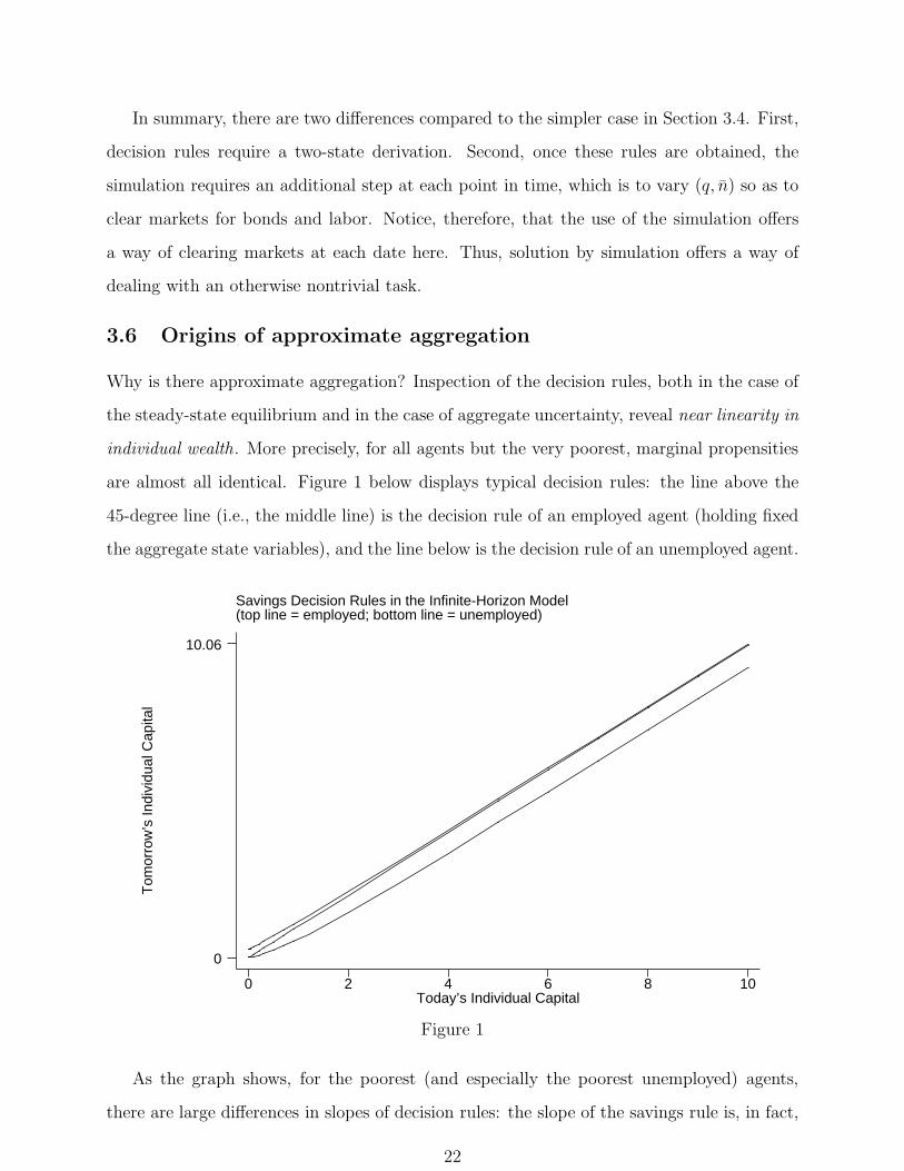
are almost all identical. Figure 1 below displays typical decision rules: the line above the

45-degree line (i.e., the middle line) is the decision rule of an employed agent (holding fixed

the aggregate state variables), and the line below is the decision rule of an unemployed agent.

Savings Decision Rules in the Infinite-Horizon Model(top line = employed; bottom line = unemployed)

Tom

orro

w’s

Indi

vidu

al C

apita

l

Today’s Individual Capital0 2 4 6 8 10

0

10.06

Figure 1

As the graph shows, for the poorest (and especially the poorest unemployed) agents,

there are large differences in slopes of decision rules: the slope of the savings rule is, in fact,

22

zero for those who are borrowing-constrained, but there is also a small region of values for

ω where slopes are positive but noticeably lower than for richer agents.

For several reasons, however, these differences in marginal propensities play only a very

minor role. First, the region where there are different marginal propensities to save is very

small. Second, the distribution of wealth is very thin in the tails and so it contains few

consumers in the region where marginal propensities are different. Third, the consumers in

left tail have, by definition, very little wealth and simply do not matter in the determination

of aggregate savings: those with the bulk of savings have wealth, and therefore (almost) have

the same marginal savings propensity. Fourth and finally, for deviations from aggregation to

be important, one needs large redistributions involving this subsegment of population, and

Γ does not seem to vary enough to make such effects quantitatively visible. In conclusion,

a number of conditions need to be satisfied to cause significant deviations from aggregation,

and none of these conditions are present in an important way.

What causes these features? In the case of the steady-state equilibrium, this near linearity

is clearly not due to boundedly rational perceptions (and it will be found to be present in

the two-period model below as well, where an equilibrium is also computed with controlled

accuracy), and the addition of price uncertainty does not change the finding. In fact, the

finding of linearity is remarkably robust to changes in the utility function: very large amounts

of risk aversion are needed to cause precautionary savings motives to make savers differ

significantly in marginal propensities. The finding seems related to other observations: the

equity premium puzzle (see Mehra and Prescott (1985)) and the low estimates for the welfare

costs of business cycles (see Lucas (1987)) both suggest that the utility functions that seem

consistent with micro data do not give large costs of bearing moderate risks.

In addition, though the presence of incomplete insurance opportunities makes agents de

facto more sensitive to shocks, precautionary savings are allowed here and they seem to be

effective in providing (partial) insurance against shocks. When an agent is allowed to save,

for given fluctuations in ǫ (labor income), the wealthier an agent is in terms of initial asset

wealth, the less important are these fluctuations to the agent. As a result, the marginal

propensity to consume ends up being determined by permanent-income considerations: for

every additional dollar of asset income, the agent consumes only the interest component and

23

keeps the principal intact, thus making the savings propensity independent of wealth for

high enough wealth levels.15 It simply turns out, then, that very little wealth is needed for

this (approximate) constancy to start to hold.

It is also possible to understand why there are few agents in the region with the very lowest

asset levels: agents do suffer from a lack of assets, because marginal utility of consumption

is very high there. Thus, with a long enough time horizon, agents save ex ante so as to avoid

ending up in this region. Preferences with higher risk aversion make being in this region

even more costly, and the distribution of wealth thus moves to the right endogenously. In

models with short enough life spans for consumers and no bequests, it is easier to find

equilibria with more agents in the left tail of the distribution; see, e.g., Gourinchas (2000)

and Storesletten, Telmer, and Yaron (2004a). However, in these cases it is still the case

that the small amounts of wealth held by these agents still make their different marginal

propensities not matter much for aggregate savings and other aggregates.

The approximate aggregation result has surprising generality for all the above reasons.

For studies that investigate the limits of approximate aggregation, see, for example, Young

(2004a), and for a discussion of a set of circumstances in which approximate aggregation

may fail in the context of overlapping-generations economies, Krueger and Kubler (2004).

The preliminary findings suggest that models that violate approximate aggregation need

parameterizations that are quite different than those in standard macroeconomic calibrations.

3.7 A sample of positive results

For illustration, we will review some properties of the basic model described above. The

purpose here is thus not to discuss the ultimate value of specific models, but rather to make

some remarks about quantitative work in this area and about what approximate aggregation

does and does not imply.

Aggregates The time series for aggregates generated by the model can be compared to

those generated by the corresponding representative-agent model. Here, a striking finding

is the robustness of the representative-agent setting: the aggregate time series are almost

identical in the two models. This fact follows rather directly from approximate aggregation:

15See Bewley (1977).

24

one can construct a representative agent—with the same preferences as those of all agents

and the same kind of budget constraint, though with labor income being the mean labor

income of all agents—and endow this agent with the aggregate (mean) capital stock, and

this agent will then save (almost exactly) as in the aggregate economy with heterogeneity.

However, as we will discuss in the context of a few examples, further extensions of the

model give different time series properties than the basic representative-agent model of Sec-

tion 2, even when approximate aggregation holds. In particular, in the extended models one

cannot identify a(n approximate) representative agent with the representative agent of the

model in Section 2.

1. Heterogeneity in discount rates The easiest way to illustrate this is perhaps the exten-

sion in Krusell and Smith (1998), where consumers are assumed to have stochastic discount

factors, and where the movements in these discount factors, like employment risk, are not

directly insurable. Thus, at any point in time there is a nontrivial distribution of discount

factors in the population. This model displays approximate aggregation, for much the same

reasons as discussed above, even though there is heterogeneity in attitudes toward saving

in the population. The added heterogeneity generates larger differences in the marginal

propensities to consume in the population, but now there is in addition an offsetting mech-

anism: more patient agents accumulate more wealth, and therefore aggregate savings are

more concentrated. Since savings com (almost) entirely from this this group, the deviations

from perfect aggregation are again extremely small. Thus, interest rates are largely pinned

down by the marginal rates of substitution of the rich, patient agents.

At the same time, however, poor and impatient agents do command a large fraction of

total income, since they work and therefore receive labor income, and this implies that aggre-

gate consumption is influenced more by the poor than are aggregate savings. In particular,

the poor look more like hand-to-mouth consumers, since their discount rates tend to be sig-

nificantly higher than the interest rate: unlike the rich, who display permanent-income-like

behavior, poor agents who receive positive income shocks consume most of the added income.

Thus, aggregate consumption and aggregate income comove more strongly than in the model

of Section 2: we tend to see more of a traditional “consumption function” here. Since there

is approximate aggregation, though, should there not be a representative-agent counterpart

25

of this setup? Perhaps, but the question then is what the preferences of such an agent would

look like.16 Instead, it seems more appropriate to think of a two-agent “shortcut” of this

model: a model with rich savers and poor workers, who do not save at all.

2. Individual vs. aggregate labor supply In an effort to make the above macroeconomic

model consistent with the estimates of labor supply in the applied labor literature, Hansen

(1985) and Rogerson (1988) assume that labor supply is indivisible: consumers can choose

either to work or not to work, so that labor supply is highly inelastic on the individual

level. Using a lottery mechanism with complete consumption insurance, they showed that

aggregate labor supply in this case would be infinitely elastic, with adjustments of total hours

taking place on the extensive margin only. Clearly, though, their assumption of complete

insurance markets is questionable (and furthermore leads to unemployed workers to have

higher utility than employed workers). Chang and Kim (2004, 2006), however, pursue the

the idea that the interaction of partial insurance and indivisible labor could generate different

aggregate implications. Incorporating indivisible labor into the kind of model developed

in the present paper, they find that indeed aggregate labor supply is significantly more

elastic in the aggregate than one might guess based on the inelastic labor supply of any

given individual. Approximate aggregation holds, but at the same time the model produces

aggregate time series behavior that is different from that in either a standard representative-

agent model with highly inelastic labor supply or in a Hansen-Rogerson economy (which

features a representative agent with quasi-linear preferences).17

3. Idiosyncratic risk and asset prices Imperfectly insurable individual risk as an explana-

tion of asset prices has been explored within the same class of models discussed here. One of

the first to explore this idea was Mankiw (1986), who studied a two-period model. Constan-

tinides and Duffie (1996), Heaton and Lucas (1996), Krusell and Smith (1997), Storesletten,

Telmer, and Yaron (2004b), and others have built infinite-horizon models to examine this pos-

sibility. Whereas Constantinides and Duffie explore assumptions under which complete an-

16One might think that the answer should be the complete-markets version of the model, but this turnsout not to be correct. For simplicity, consider the case with permanent differences in discount factors, whichis a model with much the same properties. There, the complete-markets version leads to concentration ofwealth over time among the agent with the highest discount factor—all other agents “disappear” from theeconomy in the long run. In the long run, therefore, the economy would look like a representative-agenteconomy like the one in Section 2, which we know displays very different behavior.

17For another labor-market application, see Gomes, Greenwood, and Rebelo (2001).

26

alytical characterization is possible (e.g., only permanent—fully uninsurable—idiosyncratic

shocks), the latter two papers explore quantitatively restricted settings of the sort described

in this paper, and approximate aggregation applies in each case. There are two general

findings here: the “market price of risk” increases and the risk-free rate falls. Underlying

the higher market price of risk is the assumption that idiosyncratic risk is larger in bad

times than in good times. This qualitative point, which was made in Mankiw’s early paper,

appears in Krusell and Smith’s setting in the form of unemployment risk, which is naturally

countercyclical, and in Storesletten, Telmer, and Yaron (2004c), who document and explore

the implications of countercyclical idiosyncratic wage risk.

To understand why the risk-free rate decreases, it is useful to consider a variant of the

steady-state model in Section 3.1 developed by Huggett (1993). Huggett’s model is a pure

exchange economy without aggregate uncertainty in which the only asset is a risk-free bond

in zero net supply.18 In this model, consider setting the borrowing constraint on bonds to 0:

b = 0. In such a case, the equilibrium is by necessity autarkic: the bond price must adjust

so that no consumer wants to hold positive amounts of bonds, i.e., it must be determined

by the intertemporal marginal rate of substitution of the agent who is willing to pay the

most for the safe asset.19 If the idiosyncratic shock follows a two-state Markov chain, then

it turns out that consumers with the high shock—who face the possibility of an income loss,

unlike consumers with the low shock—determine the bond price. Such a consumer’s Euler

equation can be written

q ≥ βπh|hǫ

−γh + (1 − πh|h)ǫ

−γℓ

ǫ−γh

,

which exceeds β whenever ǫh > ǫℓ, πh|h < 1, and γ > 0. Intuitively, this consumer would

like to accumulate bonds to protect himself against the possible income loss, but he cannot

because the borrowing constraint precludes consumers with low shocks from lending to him,

so to restore equilibrium in the bond market, the price of the bond must rise relative to value

of the discount factor (which equals the bond price under complete markets). Thus the risk-

free return falls. The expression above also allows us to show that as ǫh/ǫℓ grows large

(i.e., as the gap between rich and poor increases), the interest rate declines monotonically

18Huggett’s setup is obtained by setting F (z, k, n) ≡ n.19For another paper that uses this kind of modeling in an analysis of foreign exchange risk premia, see

Leduc (2002).

27

from 1/β—its value in the economy without idiosyncratic risk—to zero. Second, the less

persistent is the high endowment shock—the more likely is the income loss—the lower is the

risk-free rate. Third and finally, the risk-free rate is lower, the more risk-averse is the agent

(the higher is γ). Depending on primitives, thus, the gross risk-free return can be anywhere

in (0, 1/β).20

The effect of consumer heterogeneity on the risk-free rate can also be examined in other

contexts, such as the economies with entrepreneurial risks considered by Angeletos (2005),

Angeletos and Calvet (2004), and Covas (2005). There, entrepreneurs make investment

decisions that due to market incompleteness will be tied with their consumption decisions,

and thus any borrowing using state-uncontingent bonds will deliver a risk-free interest rate

that is disproportionately influenced by the less wealthy lucky entrepreneurs, who are more

worried about risk. We will explore this kind of setup in the context of the two-period model

below.

Inequality The second main output of this model is time series for inequality, both in

terms of wealth and consumption. Here, we only briefly note the main findings for wealth

inequality.

One can use the time-series for inequality to compute unconditional moments for the

Gini coefficient or some other measure of inequality in wealth and in consumption. The

variations in Γ are not so large that a model with aggregate shocks is really necessary for

the analysis of long-run properties, however: analysis of steady state suffices, along the lines

of the discussion in Section 3.1. There is quite a large number of papers in this general

vein, and it is broadly recognized that the present model has a difficult time generating

wealth dispersion to the extent observed in U.S. (and other) data. As an example, the Gini

coefficient for wealth in the model calibrated in Aiyagari (1994) is 0.3, whereas in the data it

is 0.8; the fraction of wealth held by the 1% richest is much less than its value in the data of

30% (see Dıaz-Gimenez et al (1997) and Rodrıguez et al (2002) for a documentation of facts

about inequality in the U.S.), and there are few agents that have very low levels of wealth.

20In a Huggett-style endowment economy with aggregate shocks, the bond price chiefly depends on theaggregate shock, and not on the higher moments of the asset distribution (recall that its first moment alwayshas to be zero); in the case with a zero-borrowing constraint, this result holds exactly. For an analysis, seeYoung (2004b).

28

A number of ways of altering the basic framework have been suggested and evaluated.

To generate a large mass of agents at the lowest levels of wealth, one can introduce a feature

common to many modern economies, namely specific welfare benefits to the very poorest

(this idea was considered in Hubbard, Skinner, and Zeldes (1995) and put into an equilibrium

model by Huggett (1996)). Thus, poor agents are given disincentives to save. To generate

extreme wealth concentration, one can follow Krusell and Smith (1998) who hypothesize

discount-rate heterogeneity and show that a small amount of such heterogeneity is sufficient

for generating realistic wealth Ginis and a large concentration of wealth among the richest;

this mechanism also helps create a class of very poor agents.

As a somewhat related mechanism, one can consider some form credit-market imperfec-

tion that implies that the rates of return on savings earned by wealthy agents is higher than

those for poor agents. It remains to be seen whether a fully microfounded setting can be con-

structed that delivers this result as an equilibrium outcome (models of costly participation

in different markets can perhaps be developed, or models where information is asymmetric

and costly to acquire); investigations with versions of increasing returns to saving can be

found in Quadrini (2000), Campanale (2005), and Cagetti and De Nardi (2004, 2005).21

Castaneda et al (2003b) pursue another approach. They formulate a steady-state model

with idiosyncratic wage-rate shocks and find that it is possible to generate large wealth

inequality without any other form of heterogeneity (i.e., without preference or rate-of-return

heterogeneity). The required wage process has drastically higher dispersion: it features a

very small probability of entering a state with enormous wages, while having strong regression

to the mean for this group.

Thus, in short, several different stories have been proposed to account for the stark

inequality in wealth, and each has shown some success. Does it matter, then, which story is

most relevant quantitatively? It does. Models with preference heterogeneity suggest that the

poor are poor because they choose to be poor, and thus welfare policy aimed at distribution

toward the poor is hard to defend on the grounds of efficiency: it is not that the lack of

21In principle, different risk attitudes between the rich and the poor can help: if wealth lowers de-facto riskaversion, then the rich earn a higher return on average, and thus become even richer. However, it is difficultfor such a mechanism to be potent quantitatively unless one departs radically from what is considered to bereasonable specifications for individual risk attitudes: a very high degree of risk aversion is needed to generatea substantial equity premium, even in the presence of wealth heterogeneity and incomplete insurance againstidiosyncratic shocks.

29

insurance markets explains poverty, but rather that some consumers choose poverty.22 In

contrast, the model where inequality is due to a wage process with very large variance predicts

that the poor are poor because they were unlucky. Based on such a model, hence, it seems

easier to argue for redistribution on efficiency grounds.23 Thus, it is important for future

research to sort out and compare these different mechanisms; we are still far from a stage

where all the properties, especially in the time-series dimension but also cross-sectionally,

have been explored for these models.

Turning now to the cyclical properties of wealth inequality, the baseline model, with or

without preference heterogeneity, predicts that measures of wealth inequality are counter-

cyclical. However, whereas the data on income inequality is quite good (for recent studies of

U.S. data, based on different sources, see Castaneda et al (2003a) on short-run fluctuations

and Piketty and Saez (2003) for a longer-run perspective), there are too few observations on

the wealth distribution for a meaningful time-series analysis of it.

3.8 Policy evaluation

Approximate aggregation does not mean that there is close to full consumption insurance;

in fact, the models considered in this paper feature substantial consumption inequality.24

Furthermore, macroeconomic policies, such as stabilization policy, influence consumption

inequality. Because the models considered in this paper allow for macroeconomic variation,

they can be used to evaluate the distributional effects of macroeconomic policies. Macroe-

conomic policy affects prices (such as wages and interest rates) through general equilibrium

channels, thereby changing the allocation of risk across consumers with different composi-

tions of financial and human wealth; we will revisit this idea formally in Section 4.1.3 below.

So far, there are only a few papers exploring these issues; one example is a set of papers ex-

ploring how the elimination of business cycle risk affects the welfare of different groups in the

economy (Atkeson and Phelan (1994), Imrohoroglu (1989), Krebs (2003), Krusell and Smith

22It should be noted that for such a stance one must assume that “discounting”, or “impatience”, is aprimitive, and not an outcome of a social or cultural process. This is not a foregone conclusion.

23Of course, the extent to which efficiency can be used as an argument in these models is somewhatunclear, since the market incompleteness has not been modelled from first principles. That is: why can thegovernment provide valuable insurance when the markets cannot?

24Moreover, Cordoba and Verdier (2005) show that the potential welfare gains from eliminating U.S.consumption inequality, relative to those from eliminating suboptimal growth and business cycles, can bevery large.

30

(1999, 2002), Mukoyama and Sahin (2005), and Storesletten, Telmer, and Yaron (2001); see

also Lucas (2003)). Additional examples include Heathcote (2005), who studies the distribu-

tional effects of shocks to taxes in an economy of the kind discussed here (where Ricardian

equivalence fails to the extent that borrowing constraints bind), and Gomes (2002), who

studies the welfare effects of countercyclical unemployment insurance.

3.9 Summing up: implications of approximate aggregation

Does approximate aggregation mean that macroeconomists might as well limit attention to

representative-agent models? For many issues, the answer is “no”: both aggregate quantities

and prices behave quite differently in many of the models discussed above than in the stan-

dard representative-agent model. We think, moreover, that more radical departures from

the representative-agent model will occur when idiosyncratic uninsurable risk is combined

with other frictions or other elements of heterogeneity. But it is premature to speculate in

this direction.25

Another point to stress is that there is significant consumption inequality in the model

with idiosyncratic risk, even in the baseline version where the wealth distribution has much

less variance than in the data. That is, approximate aggregation does not say that inequality

in consumption and wealth are eliminated by means of precautionary savings; after all, all the

consumption and wealth inequality in the present model are due to market incompleteness.

A generalization of the steady-state models of Bewley, Huggett, and Aiyagari, the present

model is also stationary: the distribution of wealth is (in all the applications in the literature,

at least) unique, so any effects of initial wealth differences among agents disappear over

time, and the long-run differences in consumption and wealth among agents are thus due to

idiosyncratic shocks and the absence of full insurance.

In addition, this class of models does deliver nontrivial and interesting implications for the

evolution of wealth and consumption inequality that are still far from completely understood.

The tools are now available to use general-equilibrium models of inequality to tackle the

empirical challenges in a serious way.

25Carroll (2000) draws a more radical conclusion than we do on this issue and pronounces a “requiem” forthe representative-agent model.

31

4 Using 2-period models

In this section we develop and analyze a series of two-period models with the aim of (i)

illustrating and further analyzing approximate aggregation; (ii) evaluating the method of

solution by simulation in a case where alternative methods are feasible; (iii) investigating

the robustness of the representative-agent model; and (iv) examining the social insurance

role of macroeconomic policy. The first model we describe shares many features with the

“big model” above but ends after two periods. The second model introduces entrepreneurs,

following Angeletos (2005), Angeletos and Calvet (2004), and Covas (2005), to study ap-

proximate aggregation in a slightly different context with additional credit-market frictions.

It also serves to illustrate a mechanism for generating a lower risk-free rate.

4.1 1998 setup, baby version

We focus on a version of the model without valued leisure. Preferences are given by u(c1) +

βE(u(c2)); we assume that u(c) has constant relative risk aversion. The technology is the

standard neoclassical one: consumption and investment are perfect substitutes in the first

period, and an aggregate investment of k2 units in period 1 delivers output kα2 + (1 − δ)k2

in period 2. There is no aggregate technology shock in the second period, but there are

idiosyncratic wage shocks (i.e., we depart somewhat from the model above in focusing on

income uncertainty due to wage, not unemployment, risk). Finally, in the first period the

resources are given exogenously; there is no production. In the second period, each consumer

is endowed with one unit of time, which he supplies inelastically.

The decentralized economy has individual budgets that read

c1 + k2 = ω and c2 = (1 + F2(k2, 1) − δ)k2 + F (k2, 1)ǫ + a.

We assume that ǫ is lognormally distributed (with mean normalized to 1), and that shocks

are independently and identically distributed across agents so that, in the second period,

the distribution of ex-post realizations of ǫs is lognormal. Moreover, we assume that the

(exogenous) distribution of ωs is lognormal; we denote this distribution Γ1 in line with the

notation in the big model.

For any initial wealth distribution Γ1, this model can be solved with arbitrary accuracy

32

using a simple guess-and-verify procedure: one guesses on k2, which implies a rental rate

and a wage rate in the second period. Based on these prices, it is straightforward to solve

the consumer’s problem, which is strictly concave, by solving a first-order condition with

one unknown: the individual’s capital holdings. One then sums up, over a large number of

agents (or integrates numerically), the savings and then checks whether the obtained number

equals k2. It is easy to show that there is a unique value for k2 that constitutes a fixed point,

and a standard Newton-Raphson algorithm converges securely to it, thus generating an

equilibrium decision rule k2 = hk(ω). Then one can repeat this for any alternative initial

wealth distribution, Γ1, and thereby obtain k2 = hk(ω, Γ1). This decision rule can now be

compared to the dynamic decision rule for savings in Section 3: it has the entire wealth

distribution as a state variable, though this distribution is exogenous here. The task, thus,

is to vary the wealth distribution Γ1 and to explore how it impacts on the macroeconomic

equilibrium. As above, the lack of insurance markets for idiosyncratic risk makes the answer

nontrivial.

4.1.1 Results for the baseline setup

We assume that utility has a relative risk aversion coefficient of 3, and the other parameters

satisfy: β (discount factor) = 0.99, α (exponent on capital in the production function) =

0.36, and δ (rate of depreciation) = 0.025. Since Γ1 is lognormal, the key variable of interest

for us is σω: the standard deviation of the initial distribution of income. Given a value

for mean wealth, does σω matter for equilibrium savings? If it (almost) does not, we have

approximate aggregation.

Table 1 summarizes the key findings.

Table 1

σǫ σǫ

k2 0 0.5 1 1/q 0 0.5 10 1.000 1.003 1.012 0 5.41% 5.40% 5.34%

σω 0.5 1.000 1.003 1.012 0.5 5.41% 5.40% 5.34%1 1.000 1.003 1.012 1 5.41% 5.40% 5.34%

The left panel in Table 1 tabulates the equilibrium capital stock, k2, as a function of the

amount of idiosyncratic risk (σǫ), horizontally, and the amount of initial wealth dispersion

(σω), vertically, and the right panel tabulates the interest rate as a function of the same

33

variables. We normalize k2 so that it is 1 in the case of no idiosyncratic risk (the first

column): in this case, since preferences admit exact aggregation, and we indeed see that

the dispersion of initial wealth does not influence total savings. In the second column, total

savings are higher since there is now idiosyncratic risk: there is some precautionary savings.

However, looking down rows in the second column, we see identical numbers: the amount

of initial wealth dispersion does not seem to influence total savings, even though there are

incomplete markets. Here, in fact, it is possible to detect small differences—if one examines

more significant digits. But there is, clearly, approximate aggregation. In fact, all columns

have identical numbers up to 4 significant digits, simply revealing no economically significant

aggregate effects of wealth inequality on total savings or, as seen in the right panel, on interest

rates.

Table 1 also shows that the representative-agent model is rather robust to the intro-

duction of idiosyncratic risk in this case. The top left corners of the two panels show the

representative-agent model: the model with no idiosyncratic risk and no wealth dispersion.

But in fact all four entries in the first column are identical because preferences admit exact

aggregation over initial wealth in the absence of idiosyncratic shocks. In terms of the interest

rate, we thus see that the presence of uninsurable risk, and wealth inequality, does not lower

the interest rate by more than 7 basis points (i.e., seven hundredths of one percent).

Under the surface of the aggregates in Table 1, there is significant consumption inequality

and, in addition, consumption risk. Thus, approximate aggregation does not imply an

elimination of fluctuations in consumption: “self-insurance” using capital is not capable of

doing this. Nonetheless, self-insurance, at least given the preferences considered here and

in most of the macroeconomic literature, is very effective in insuring consumers in utility

terms. That is, the remaining consumption risk just does not hurt consumers enough to

change their overall attitudes toward saving much, and hence aggregate savings and interest

rates are hardly influenced at all by idiosyncratic risk.

The effectiveness of self-insurance is reflected in consumers’ decision rules, as depicted

in Figure 2. The top line is a typical decision rule with partial insurance. The bottom line

provides a point of comparison: it is the decision rule of a consumer who faces the equilibrium

prices from the model with partial insurance but has a complete set of assets to insure fully

34

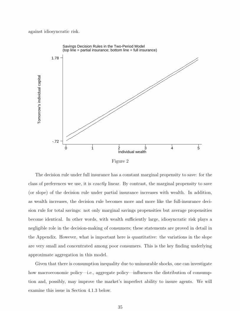
against idiosyncratic risk.

Savings Decision Rules in the Two-Period Model(top line = partial insurance; bottom line = full insurance)

Tom

orro

w’s

indi

vidu

al c

apita

l

Individual wealth0 1 2 3 4 5

-.72

1.78

Figure 2

The decision rule under full insurance has a constant marginal propensity to save: for the

class of preferences we use, it is exactly linear. By contrast, the marginal propensity to save

(or slope) of the decision rule under partial insurance increases with wealth. In addition,

as wealth increases, the decision rule becomes more and more like the full-insurance deci-

sion rule for total savings: not only marginal savings propensities but average propensities

become identical. In other words, with wealth sufficiently large, idiosyncratic risk plays a

negligible role in the decision-making of consumers; these statements are proved in detail in

the Appendix. However, what is important here is quantitative: the variations in the slope

are very small and concentrated among poor consumers. This is the key finding underlying

approximate aggregation in this model.

Given that there is consumption inequality due to uninsurable shocks, one can investigate

how macroeconomic policy—i.e., aggregate policy—influences the distribution of consump-

tion and, possibly, may improve the market’s imperfect ability to insure agents. We will

examine this issue in Section 4.1.3 below.

35

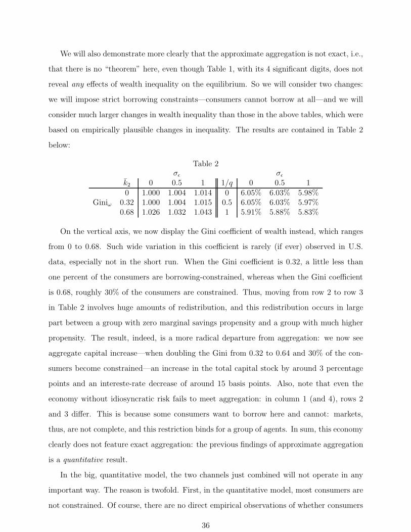
We will also demonstrate more clearly that the approximate aggregation is not exact, i.e.,

that there is no “theorem” here, even though Table 1, with its 4 significant digits, does not

reveal any effects of wealth inequality on the equilibrium. So we will consider two changes:

we will impose strict borrowing constraints—consumers cannot borrow at all—and we will

consider much larger changes in wealth inequality than those in the above tables, which were

based on empirically plausible changes in inequality. The results are contained in Table 2

below:

Table 2σǫ σǫ

k2 0 0.5 1 1/q 0 0.5 10 1.000 1.004 1.014 0 6.05% 6.03% 5.98%

Giniω 0.32 1.000 1.004 1.015 0.5 6.05% 6.03% 5.97%0.68 1.026 1.032 1.043 1 5.91% 5.88% 5.83%

On the vertical axis, we now display the Gini coefficient of wealth instead, which ranges

from 0 to 0.68. Such wide variation in this coefficient is rarely (if ever) observed in U.S.

data, especially not in the short run. When the Gini coefficient is 0.32, a little less than

one percent of the consumers are borrowing-constrained, whereas when the Gini coefficient

is 0.68, roughly 30% of the consumers are constrained. Thus, moving from row 2 to row 3

in Table 2 involves huge amounts of redistribution, and this redistribution occurs in large

part between a group with zero marginal savings propensity and a group with much higher

propensity. The result, indeed, is a more radical departure from aggregation: we now see

aggregate capital increase—when doubling the Gini from 0.32 to 0.64 and 30% of the con-

sumers become constrained—an increase in the total capital stock by around 3 percentage

points and an intereste-rate decrease of around 15 basis points. Also, note that even the

economy without idiosyncratic risk fails to meet aggregation: in column 1 (and 4), rows 2

and 3 differ. This is because some consumers want to borrow here and cannot: markets,

thus, are not complete, and this restriction binds for a group of agents. In sum, this economy

clearly does not feature exact aggregation: the previous findings of approximate aggregation

is a quantitative result.

In the big, quantitative model, the two channels just combined will not operate in any

important way. The reason is twofold. First, in the quantitative model, most consumers are

not constrained. Of course, there are no direct empirical observations of whether consumers

36

have “binding” borrowing constraints, so it is possible that indeed a large fraction of con-

sumers are constrained; however, though there are disagreements, most empirical researchers

would probably set the fraction of households with binding constraints at a number much

lower than 30%. Second, in Table 2, we exogenously change the wealth distribution from

one with a Gini of 0.32 to one of 0.64, thus effectuating a huge redistribution across the

population. Such huge redistributions simply do not occur in the data, and they clearly

do not occur in the big model either; the model roughly, at least, reproduces the wealth

distribution dynamics.

4.1.2 Assessing solution by simulation

The results in the previous section are obtained with controlled—and for the numbers we

report, very high—accuracy. We now use the knowledge of what the “exact” equilibrium is

in order to assess how solution by simulation works in the 2-period model. For this purpose,

let the mean and variance of the (lognormal) wealth distribution be random variables drawn

from known distributions. Consumers are now assumed to be boundedly rational: their

perceptions are given by a view of what k2 is that depends only on mean wealth. We thus

specify, as in the big model, a mapping from mean wealth today to future wealth that is

simple; it is parameterized by θ, and we choose θ so that, given the parametric form, it gives

the best fit for consumers. To pin down the parameters θ of this “forecasting rule”, solution

by simulation is employed: (i) we draw simulated values for the mean and variance of the

wealth distribution, thus for each draw obtaining the value of k2 implied by the initial guess

on θ; (ii) we use the simulated data to estimate a new value for θ; and (iii) we iterate to

convergence and assess the fit of the forecasting rule.

Notice that the solution by simulation, by construction, allows the possibility of a self-

fulfilling prophecy. That is, agents’ behavior are based on certain (boundedly rational)

perceptions, and then one could imagine that their implied behavior, due to the imperfect

perceptions, somehow, would (almost) confirm these perceptions. Fully rational expecta-

tions, at least in models with complete markets, eliminate self-fulfilling equilibria, and we do

not expect there to be multiple expectational equilibria in the big model; in the two-period

model considered in this section, we can prove that the equilibrium is unique. The point,

thus, is that without rational expectations, little is known regarding uniqueness, which is

37

why it is important to examine the issue here, where we know the exact equilibrium and can

compare it to the equilibrium we find using boundedly rational perceptions and solution by

simulation.

We let the mean and standard deviation of the wealth distribution vary by 10%; the

average wealth Gini is 0.51. The results can be summarized in two observations. First, in all

cases, the fit of the forecasting rule is nearly perfect: R2 ≈ 0.99999, with a residual standard

deviation of about 0.04%.26 Second, the solution by simulation was extremely close to the

exact solution: the deviations are on the order of 0.001%!

Thus, we conclude that the solution found by solution by simulation is not produced due

to a self-fulfilling prophecy, as expected. The basic reason why our algorithm works really

is the fundamental workings of this model: decision rules are extremely close to linear, and

they are linear because very little wealth suffices to insure very well in utility terms.

4.1.3 Illustrating the social insurance role of macro policy

One of the interesting aspects of macroeconomic models with heterogeneous consumers is

that they allow us to trace effects of policy across different consumer groups. Thus, one can

use these models to examine the effects—positive and normative—of government insurance

policy, aimed explicitly at improving on market outcomes from the insurance perspective.

Perhaps more interestingly, the model also makes clear how purely aggregate policy actually

may have nontrivial and interesting effects on inequality. Here we will illustrate the effects

of a tax on investment using a simple example from Davila, Hong, Krusell, and Rıos-Rull

(2005).

For the sake of the argument, assume that there is no initial wealth inequality in the

two-period model: ω is the same for all consumers. Moreover, suppose that ǫ can only

take on two values (as in the employed/unemployed case): ǫ1 occurs with probability π. A

competitive equilibrium is now simply a vector (k2, r, w) such that (i) k2 solves

maxk∈[0,y]

u(ω − k) + β (πu(rk + we1) + (1 − π)u(rk + we2))

and (ii) r = F2(k2, n2) and w = F2(k2, n2), with n2 = πe1 + (1 − π)e2.

26When we use the extreme changes in wealth inequality, the lowest recorded R2 was 0.99919.

38

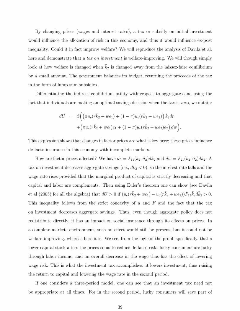
By changing prices (wages and interest rates), a tax or subsidy on initial investment

would influence the allocation of risk in this economy, and thus it would influence ex-post

inequality. Could it in fact improve welfare? We will reproduce the analysis of Davila et al.

here and demonstrate that a tax on investment is welfare-improving. We will though simply

look at how welfare is changed when k2 is changed away from the laissez-faire equilibrium

by a small amount. The government balances its budget, returning the proceeds of the tax

in the form of lump-sum subsidies.

Differentiating the indirect equilibrium utility with respect to aggregates and using the

fact that individuals are making an optimal savings decision when the tax is zero, we obtain:

dU = β(

(

πuc(rk2 + we1) + (1 − π)uc(rk2 + we2))

k2dr

+(

πuc(rk2 + we1)e1 + (1 − π)uc(rk2 + we2)e2

)

dw)

.

This expression shows that changes in factor prices are what is key here; these prices influence

de-facto insurance in this economy with incomplete markets.

How are factor prices affected? We have dr = F11(k2, n2)dk2 and dw = F21(k2, n2)dk2. A

tax on investment decreases aggregate savings (i.e., dk2 < 0), so the interest rate falls and the

wage rate rises provided that the marginal product of capital is strictly decreasing and that

capital and labor are complements. Then using Euler’s theorem one can show (see Davila

et al (2005) for all the algebra) that dU > 0 if (uc(rk2 + we1)− uc(rk2 + we2))F11k2dk2 > 0.

This inequality follows from the strict concavity of u and F and the fact that the tax

on investment decreases aggregate savings. Thus, even though aggregate policy does not

redistribute directly, it has an impact on social insurance through its effects on prices. In

a complete-markets environment, such an effect would still be present, but it could not be

welfare-improving, whereas here it is. We see, from the logic of the proof, specifically, that a

lower capital stock alters the prices so as to reduce de-facto risk: lucky consumers are lucky

through labor income, and an overall decrease in the wage thus has the effect of lowering

wage risk. This is what the investment tax accomplishes: it lowers investment, thus raising

the return to capital and lowering the wage rate in the second period.

If one considers a three-period model, one can see that an investment tax need not

be appropriate at all times. For in the second period, lucky consumers will save part of

39

their proceeds from having a high wage outcome. This means that a subsidy to investment

may be appropriate at that point in time: it will raise w3 and lower r3, thus reducing the

de-facto risk in period-2 wages. Of course, if period-3 wages are also random, a period-2

investment subsidy would increase risk from that perspective, so whether a subsidy or a tax

is appropriate is a quantitative matter in a longer-horizon model. Davila et al. indeed show

that steady-state capital stocks are too high for some calibrations and too low for others.

Quantitatively, they argue, based on a calibration for the wealth distribution based on luck,

not discount-factor heterogeneity, that a subsidy looks most appropriate.

Finally, let us comment briefly on a methodological aspect of the kind of welfare analysis

undertaken here. In our analysis, markets are incomplete by assumption: the restrictions

consumers face in being able to insure against the idiosyncratic shocks are not derived from

first principles based on explicit frictions, such as asymmetric information or enforcement

problems. This means that welfare experiments are hazardous, because one might imagine

that a change in policy would also change the market structure: economic agents would

change their behavior in response to the new policy. That is, one could raise a form of

“Lucas critique” here.

Indeed, the recent literature on dynamic contracting is in large part motivated by such

concerns; see Kocherlakota (2005). One of the goals of that literature is to “endogenously

derive” what we perceive as empirically plausible market imperfections, and also to try to

explain observed taxation patterns in terms of optimal insurance policy for these dynamic

environments (thus building intertemporal versions of the work of Mirrlees (1971)). This

work is promising and very interesting from the present perspective, since it delivers impli-

cations for inequality. However, because it is still in its infancy, its most successful attempts

are not that close to what we perceive as a realistic setting from the perspective of typical

households in the data. In contrast, the model we use here seems much more descriptively

accurate—it is what empirical microeconomic researchers use, and also seems appealing from

the (admittedly limited) perspective of our own lives. Therefore, it does seem reasonable to

examine its welfare properties. We also think that the mechanisms emphasized here can be

evaluated on their own terms to some extent; for example, the price manipulations a gov-

ernment would undertake according to the results discussed above are intuitive. Hopefully,

40

a more complete analysis will be possible in the future, and it is far from impossible that

the mechanisms we discuss here also play an important role in such an analysis.

4.2 The risk-free rate: an economy with entrepreneurs

Finally, we consider a model which is a step further from the neoclassical growth model:

production does not take place using a ubiquitous technology. Put differently, factors of

production are not costlessly mobile across production sites. We will use this setup to

demonstrate that, with otherwise unchanged assumptions—idiosyncratic shocks with no di-

rect insurance available, and initial wealth inequality—some new features materialize: the

asset-pricing implications are far from those of the neoclassical economy.

We look at a two-period version of Covas (2005), which itself can be viewed as a version

of Angeletos (2005) where entrepreneurs cannot hire labor. More precisely, entrepreneurs

invest in capital in period 1 and face idiosyncratic productivity risk in the second period:

if an entrepreneur invests k, his second-period output is ǫkα, with ǫ lognormal and iid.27

As in the previous two-period model, there is then no aggregate risk in the second period.

Capital is immobile ex post: two entrepreneurs with different realizations for their ǫs cannot

increase output by letting capital move towards the more productive entrepreneur. Moreover,

the production technology makes clear that the amount of labor input is also fixed (at a

normalized value of one); this could reflect an assumption that the entrepreneur himself is

an unsubstitutable input, or it could reflect an assumption that the labor input takes even

longer to reallocate across production sites than does the capital input. The productivity risk

cannot be insured against with any direct insurance markets; moreover, there is a “financing

friction” in that the only individual capable of investing in an entrepreneur’s technology is

the entrepreneur himself. That is, equity cannot be traded.

The budget of a typical entrepreneur reads:

c1 + k2 + qb2 = ω and c2 = ǫkα2 + b2 + a.

Thus, the entrepreneur can borrow, or lend, at a risk-free interest rate 1/q.

27Notice that risk in some sense is different here: it is complementary with the investment choice. Thatis, higher investment increases individual risk. Conversely, zero investment, which is feasible, allows risk tobe eliminated entirely.

41

Table 3 summarizes the equilibrium behavior of this model for a range of parameter

settings.

Table 3σǫ σǫ

k2 0 0.5 1 1/q 0 0.5 10 1.000 1.006 1.020 0 5.41% 4.57% 2.74%

σω 0.5 1.000 1.006 1.020 0.5 5.41% 4.57% 2.74%1 1.000 1.006 1.020 1 5.41% 4.57% 2.74%

Table 3 illustrates two points quite clearly: (i) approximate aggregation obtains again;

and (ii) the model has very different implications than its representative-agent counterpart.

As for the first point, again all the numbers in any given column are the same: differences

appear only if more significant digits are included. As for the effects of entrepreneurial risk on

asset prices, we now see very large effects. With higher idiosyncratic risk, interest rates fall

drastically—Table 3 reveals a fall of over 2.5 percentage points. Even though decision rules

for investment/savings are quite linear in wealth here in the relevant range, the demand for

bonds is influenced significantly by the poorer entrepreneurs who value insurance more. The

rich entrepreneurs invest up to an amount that roughly equalizes the expected return from

investment with the risk-free rate, whereas the poorer entrepreneurs do not, thus stopping

short: for them, the marginal resources otherwise invested are better saved at a safe rate.

Thus, they value consumption in the future more on the margin: they are willing to pay

more for a bond, every thing else equal.

5 Conclusions and final remarks

We have reviewed what has become a rather active quantitative research area in the inter-

section of macroeconomics and the applied consumption-savings, labor, and finance/asset-

pricing literatures. The overall idea is to use available insights from these applied literatures

to construct aggregate models with realistic underpinnings. Besides performing an impor-

tant “robustness check” on the standard representative-agent macroeconomic model, this

research allows an understanding of the equilibrium determination of inequality. Moreover,

it opens up an interesting avenue for exploring effects of macroeconomic policy—namely,

on the cross-section of consumers, and on their ability to insure risk effectively—that have

hitherto been ignored, or abstracted from.

42

Much of the work reviewed here emphasizes the methodological advances. In particular,

we illustrate and explain the finding of approximate aggregation, a feature of economies

with heterogeneous agents that has greatly expanded the class of models that can feasibly

be studied. The boundaries of the applicability of approximate aggregation are far from

known; so far, we know of no quantitatively convincing models with large departures from

aggregation, but our imagination is admittedly limited and we foresee important examples of

such phenomena to be discovered in future research. Indeed, we think that the exploration

of this boundary is an important task for the future work in this area.

Finally, we develop a two-period model, in Section 4, which not only is useful for illus-

tration, we think, but also for conducting “pilot studies” within this area. Thus, one likely

obtains important insights about whether approximate aggregation will hold, and about

what interesting features a model might have, by first investigating a two-period model of

the sort we examine here.

Almost by necessity, the work on dynamic macroeconomic equilibrium models requires

heavy use of numerical methods, but computers are powerful now and the numerical methods

available are becoming standard fare in many graduate programs all over the world. The

original model in Krusell and Smith (1998) can now be solved in a matter of minutes using

our own code, and that code was not written for the purposes of maximizing speed.

It seems obvious to us that many exciting issues are now open for exploration using the

kinds of theoretical structures discussed here. There is ongoing work that attempts to inte-

grate the present model with risk-averse individuals and incomplete asset markets with more

explicit models of labor market frictions, along the lines of Mortensen and Pissarides (1994),

where wage/employment shocks are endogenous. The work on policy—examining macroeco-

nomic policy from a social insurance perspective, and comparing it with, and looking at how

it complements, more explicit social insurance/welfare policy—has also begun. Similarly,

there is some work that incorporates firm heterogeneity, credit-market frictions, and immo-

bility of input factors—which appear to be plausible sources of idiosyncratic shocks both to

workers and firm owners—but there is much to do. Here, our two-period example economy

of Section 4.2 is an example: it has not yet been solved in an infinite-horizon version. This

illustrates the value of using the two-period model for pilot studies: we have identified a

43

feasible paper to be written, namely the examination of aggregate risk in environments like

those studied by Covas (2005) and Angeletos (2005): approximate aggregation will almost

certainly hold there, and the asset-pricing implications of such a model seem quite promising.

In contrast, there is very little work examining further elements of heterogeneity, such

as the heterogeneity of consumption goods. Here, one may not expect that distinguishing

between different kinds of cereal to be an important step forward for macroeconomics, but it

may be important to makes distinctions between broad categories: nondurable consumption,

durable consumption, services, and housing consumption. Further, preference heterogeneity

seem very important to explore: if preferences for cereal are as different as they are (Tony

likes Grape Nuts and Per Mueslix), then isn’t it reasonable to expect differences between

consumers also in dimensions that appear to be of greater macroeconomic relevance, such as

their attitudes toward risk and saving?

Finally, we expect that work on asymmetric information—different views among con-

sumers and firms regarding future events—to be an important element of future macroeco-

nomic models; after all, it seems that most of real-world asset-market trade and the asso-

ciated investments are not just explained by risk-sharing or liquidity needs. Another area

with which the quantitative literature on consumer heterogeneity has had relatively little

overlap so far is monetary economics; recent work by Doepke and Schneider (2004) suggests

that monetary policy shocks may have important consequences for inequality.

A very final point is that, with computer speed still growing at a significant rate, we

foresee the possibility that the class of models studied here can be estimated structurally.

Here as well, methodological work, both in numerical analysis and statistics, is expected to

be an important component for the next several years.

44

REFERENCES

Aiyagari, S.R. (1994), “Uninsured Idiosyncratic Risk and Aggregate Saving”, Quarterly Jour-

nal of Economics 109, 659–684.

Allen, F. (1985), “Repeated Principal-Agent Relationships with Borrowing and Lending”,

Economics Letters 17, 27–31.

Altug, S. and P. Labadie (1994), Dynamic Choice and Asset Markets, Academic Press.

Angeletos, G.-M. (2005), “Uninsured Idiosyncratic Investment Risk and Aggregate Saving”,

manuscript.

Angeletos, G.-M. and L. Calvet (2004), “Idiosyncratic Production Risk, Growth and the

Business Cycle”, manuscript (forthcoming in Journal of Monetary Economics).

Atkeson, A., and C. Phelan (1994), “Reconsidering the Costs of Business Cycles with In-

complete Markets”, in: S. Fischer and J. Rotemberg, eds., NBER Macroeconomics Annual

1994 , 187–207.

Attanasio, O. (2005), “Consumption”, Chapter 11 in J. Taylor and M. Woodford, eds.,

Handbook of Macroeconomics, North-Holland, 741–812.

Bewley, T. (undated), “Interest Bearing Money and the Equilibrium Stock of Capital”,

manuscript.

Bewley, T. (1977), “The Permanent Income Hypothesis: A Theoretical Formulation”, Jour-

nal of Economic Theory 16, 252–292.

Blundell, R. and T. Stoker (2003), “Models of Aggregate Economic Relationships that Ac-

count for Heterogeneity”, manuscript (forthcoming in Handbook of Econometrics, Volume

6).

Browning, M., L. P. Hansen, and J. Heckman (2005), “Micro Data and General Equilibrium

Models”, Chapter 8 in J. Taylor and M. Woodford, eds., Handbook of Macroeconomics,

North-Holland, 543–633.

Cagetti, M. and M. De Nardi (2004), “Taxes, Entrepreneurship, and Wealth”, manuscript.

Cagetti, M. and M. De Nardi (2005), “Entrepreneurship, Frictions, and Wealth”, manuscript.

Campanale, C. (2005), “Increasing Return to Savings and Wealth Inequality”, manuscript.

Carroll, C. (2000), “Requiem for the Representative Consumer? Aggregate Implications of

Microeconomic Consumption Behavior”, American Economic Review, Papers and Proceed-

ings 90, 110–115.

45

Carroll, C. and M. Kimball (1996), “On the Concavity of the Consumption Function”,

Econometrica 64, 981–992.

Castaneda, A., J. Dıaz-Gimenez, and J.-V. Rıos-Rull (2003a), “Exploring the Income Dis-

tribution Business Cycle Dynamics”, Journal of Monetary Economics 42, 93–130.

Castaneda, A., J. Dıaz-Gimenez, and J.-V. Rıos-Rull (2003b), “Accounting for the U.S.

Earnings and Wealth Inequality”, Journal of Political Economy 111, 814–857.

Chang, Y. and S.-B. Kim (2004), “Heterogeneity and Aggregation in the Labor Market:

Implications for Aggregate Preference Shifts”, manuscript.

Chang, Y. and S.-B. Kim (2006), “From Individual to Aggregate Labor Supply: A Quanti-

tative Analysis Based on a Heterogeneous-Agent Macroeconomy”, manuscript (forthcoming

in International Economic Review).

Chatterjee, S., D. Corbae, M. Nakajima, and J.-V. Rıos-Rull (2002), “A Quantitative Theory

of Unsecured Consumer Credit with Risk of Default”, manuscript.

Cole, H. and N. Kocherlakota (2001), “Efficient Allocations with Hidden Income and Hidden

Storage”, Review of Economic Studies 68, 523–542

Constantinides, G.M. and D. Duffie (1996), “Asset Pricing with Heterogeneous Consumers”,

Journal of Political Economy 104, 219–240.

Cooley, T. and V. Quadrini (2006), “Monetary Policy and the Financial Decisions of Firms”,

Economic Theory 27, 243–270.

Cooley, T. R. Marimon, and V. Quadrini (2004), “Aggregate Consequences of Limited Con-

tract Enforceability”, Journal of Political Economy 112, 817–847.

Cordoba, J.C. and G. Verdier (2005), “Lucas vs. Lucas: On Inequality and Growth”,

manuscript.

Covas, F. (2005), “Uninsured Idiosyncratic Production Risk with Borrowing Constraints”,

manuscript (forthcoming in the Journal of Economic Dynamics and Control).

Davila, J. J. Hong, P. Krusell, and J.-V. Rıos-Rull (2005), “Constrained Efficiency in the

Neoclassical Growth Model with Uninsurable Idiosyncratic Shocks”, manuscript.

Den Haan, W.J. (1997), “Solving Dynamic Models with Aggregate Shocks and Heterogeneous

Agents”, Macroeconomic Dynamics 1, 355-386.

Den Haan, W.J. and A. Marcet (1990), “Solving a Growth Model by Parameterized Expec-

tations”, Journal of Business and Economic Statistics 8, 31–34.

46

Dıaz-Gimenez, J., V. Quadrini, and J.-V. Rıos-Rull (1997), “Dimensions of Inequality: Facts

on the U.S. Distributions of Earnings, Income, and Wealth”, Federal Reserve Bank of Min-

neapolis Quarterly Review 21, 3–21.

Doepke, M. and M. Schneider (2004), “Real Effects of Inflation through the Redistribution

of Nominal Wealth”, manuscript.

Gomes, J. (2002), “The Right Stimulus: Extended Unemployment Insurance Benefits or Tax

Cuts?”, manuscript.

Gomes, J., J. Greenwood, and S. Rebelo (2001), “Equilibrium Unemployment”, Journal of

Monetary Economics 48, 109–152.

Gourinchas, P.-O. (2000), “Precautionary Saving, LifeCycle, and Macroeconomics”, manu-

script.

Hansen, G.D. (1985), “Indivisible Labor and the Business Cycle”, Journal of Monetary

Economics 16, 309–27.

Heathcote, J. (2005), “Fiscal Policy with Heterogeneous Agents and Incomplete Markets”,

Review of Economic Studies 72, 161–188.

Heaton, J. and D.J. Lucas (1996), “Evaluating the Effects of Incomplete Markets on Risk

Sharing and Asset Pricing”, Journal of Political Economy 104, 443–487.

Hubbard, R.G., J. Skinner, and S.P. Zeldes (1995), “Precautionary Saving and Social Insur-

ance”, Journal of Political Economy 103, 360–399.

Huggett, M. (1993), “The Risk-Free Rate in Heterogeneous-Agents, Incomplete Markets

Economies”, Journal of Economic Dynamics and Control 17, 953–969.

Huggett, M. (1996), “Wealth Distribution in Life-Cycle Economies”, Journal of Monetary

Economics 38, 469–494.

Huggett, M. (1997), “The One-Sector Growth Model with Idiosyncratic Shocks: Steady

States and Dynamics”, Journal of Monetary Economics 39, 385–403.

Imrohoroglu, A. (1989), “The Cost of Business Cycles with Indivisibilities and Liquidity

Constraints”, Journal of Political Economy 97, 1364–1383.

Khan, A. and J. Thomas (2003), “Nonconvex Factor Adjustments in Equilibrium Business

Cycle Models: Do Nonlinearities Matter?”, Journal of Monetary Economics 50, 331–360.

Khan, A. and J. Thomas (2005), “Inventories and the Business Cycle: An Equilibrium

Analysis of (S,s) Policies”, manuscript.

47

Kocherlakota, N. (2005), “Advances in Dynamic Optimal Taxation”, manuscript.

Krebs, T. (2003), “Growth and Welfare Effects of Business Cycles in Economies with Id-

iosyncratic Human Capital Risk”, Review of Economic Dynamics 6, 846–868.

Krueger, D. and F. Kubler (2004), “Computing Equilibrium in OLG Models with Stochastic

Production”, Journal of Economic Dynamics and Control 28, 1411–1436.

Krusell, P. and A.A. Smith, Jr. (1997), “Income and Wealth Heterogeneity, Portfolio Selec-

tion, and Equilibrium Asset Returns”, Macroeconomic Dynamics 1, 387–422.

Krusell, P. and A.A. Smith, Jr. (1998), “Income and Wealth Heterogeneity in the Macroe-

conomy,” Journal of Political Economy 106, 867–896.

Krusell, P. and A.A. Smith, Jr. (1999), “On the Welfare Effects of Eliminating Business

Cycles,” Review of Economic Dynamics 2, 245–272.

Krusell, P. and A.A. Smith, Jr. (2002), “Revisiting the Welfare Effects of Eliminating Busi-

ness Cycles”, manuscript.

Leduc, S. (2002), ”Incomplete Markets, Borrowing Constraints, and the Foreign Exchange

Risk Premium”, Journal of International Money and Finance 21, 957–80.

Lucas, Jr., R.E. (1976), “Econometric Policy Evaluation: A Critique”, in: Meltzer, A. and

K. Brunner, eds., The Phillips Curve and Labor Markets (Vol. 1 of Carnegie-Rochester

Conference Series on Public Policy), 19–46.

Lucas, Jr., R.E. (1987), Models of Business Cycles (Basil Blackwell).

Lucas, Jr., R.E. (2003), “Macroeconomic Priorities”, American Economic Review 93, 1–14.

Mankiw, N.G. (1986), “The Equity Premium and the Concentration of Aggregate Shocks”,

Journal of Financial Economics 17, 211–219.

Mehra, R. and E.C. Prescott (1985), “The Equity Premium: A Puzzle”, Journal of Monetary

Economics 15, 145–161.

Miao, J. (2002), “Stationary Equilibria of Economies with a Continuum of Heterogeneous

Consumers”, manuscript.

Mirrlees, J. (1971), “An Exploration in the Theory of Optimum Income Taxation”, Review

of Economic Studies 38, 175–208.

Mortensen, D. and C.A. Pissarides (1994), “Job Creation and Job Destruction in the Theory

of Unemployment”, Review of Economic Studies 61, 397–415.

Mukoyama, T. and A. Sahin (2005), “Costs of Business Cycles for Unskilled Workers”,

48

manuscript (forthcoming in Journal of Monetary Economics.

Obiols-Homs, F. (2003), “Incomplete Unemployment Insurance and Aggregate Fluctua-

tions”, Review of Economic Dynamics 6, 602–636.

Quadrini, V. (2000), “Entrepreneurship, Saving, and Social Mobility”, Review of Economic

Dynamics 45, 1–40.

Piketty, T. and E. Saez (2003), “Income Inequality in the United States: 1913-1998”, Quar-

terly Journal of Economics 118, 1–39.

Rıos-Rull, J.-V. (2001), “Computation of Equilibria in Heterogeneous Agent Models”, in Ma-

rimon, R. and A. Scott, eds., Computational Methods for the Study of Dynamic Economies:

An Introduction, Oxford University Press, 238–280.

Rodrıguez, S.B., J. Dıaz-Gimenez, V. Quadrini, and J.-V. Rıos-Rull (2002), “Updated Facts

on the U.S. Distributions of Earnings, Income, and Wealth”, Federal Reserve Bank of Min-

neapolis Quarterly Review 26, 2–35.

Rogerson, R. (1988), “Indivisible Labor, Lotteries and Equilibrium”, Journal of Monetary

Economics 21, 3–16.

Storesletten, K., C. Telmer, and A. Yaron (2001), “The Welfare Costs of Business Cycles

Revisited: Finite Lives and Cyclical Variation in Idiosyncratic Risk”, European Economic

Review 45, 1311–1339.

Storesletten, K., C. Telmer, and A. Yaron (2004a), “Consumption and Risk Sharing over the

Life Cycle”, Journal of Monetary Economics 51, 609–633.

Storesletten, K., C. Telmer, and A. Yaron (2004b), “Asset Pricing with Idiosyncratic Risk

and Overlapping Generations”, manuscript.

Storesletten, K., C. Telmer, and A. Yaron (2004c), “Cyclical Dynamics in Idiosyncratic

Labor-Market Risk”, Journal of Political Economy 112, 695–717.

Young, E. (2004a), “Approximate Aggregation: An Obstacle Course for the Krusell-Smith

Algorithm”, manuscript.

Young, E. (2004b), “Solving the Heterogeneous-Agent Stochastic Growth Model with Finite

Forecasting Restrictions”, manuscript.

Zhang, L. (2005), “The Value Premium”, Journal of Finance 60, 67–103.

49

Appendix: approximate linearity in the 2-period model

Consider first the case with full insurance; let the price of a state-contingent bond paying

1 in state ǫ and zero otherwise be qf(ǫ), where f(ǫ) is the probability density associated to

state ǫ (the distribution function is denoted F (ǫ), with an expected value of ǫ); thus, for

comparison with the incomplete-markets economy, we assume actuarially fair insurance and

that the price of a riskless bond is q. It is straightforward in this case to show that a(ω, ǫ),

the optimal holding of this state-contingent bond, must satisfy

a(ω, ǫ) =ω + q(ǫ − ǫ) − ǫ

(

qβ

) 1

γ

q +(

qβ

) 1

γ

.

Thus, this amount is linear in ω, and therefore so is the total amount of bonds:

∫

a(ω, ǫ)F (dǫ) =ω − ǫ

(

qβ

) 1

γ

q +(

qβ

) 1

γ

.

Thus, the marginal propensity to buy bonds is 1/(q+(q/β)1/γ), and as wealth goes to infinity,

this also equals the average propensity (i.e., bond holdings over total initial wealth).

In the economy with only a riskless bond, the first-order condition reads

q

β(ω − qa(ω))−γ =

∫

(ǫ + a(ω))−γ F (dǫ)

for all ω. This allows us to see that a(ω) must be increasing. Take the derivative with respect

to ω and obtain

q

β(ω − qa(ω))−γ−1 (1 − a′(ω)) =

(∫

(ǫ + a(ω))−γ−1 F (dǫ))

a′(ω).

These two equations can be rewritten as

q

β=∫

(

ω − qa(ω)

ǫ + a(ω)

)γ

F (dǫ) (2)

andq

β

1 − a′(ω)

a′(ω)=∫

(

ω − qa(ω)

ǫ + a(ω)

)γ+1

F (dǫ). (3)

Let s(ω, ǫ) ≡ ω−qa(ω)ǫ+a(ω)

; s is the ratio of current to future consumption. It is positive and

decreasing in ǫ. One can show that there exists an ǫ∗ such that s1(ω, ǫ∗) = 0, s1(ω, ǫ) > 0

for all ǫ > ǫ∗, and s1(ω, ǫ) < 0 for all ǫ < ǫ∗.28 Now we can write equations (2) and (3) as

q

β=∫

s(ω, ǫ)γF (dǫ) (4)

28To see this, first note that the derivative of ω−qa(ω)ǫ+a(ω) equals (1−qa

′(ω))(ǫ+a)−(ω−qa(ω))a′(ω)(ǫ+a)2 =

1ǫ+a(ω)

(

1 − a′(ω) qǫ+ω

ǫ+a(ω)

)

= 1ǫ+a(ω)

(

1 − qa′(ω) qǫ+ω

qǫ+qa(ω)

)

. This expression cannot be zero for more than

one value of ǫ; call that value ǫ∗. Moreover, since ω > qa(ω), qǫ+ω

qǫ+qa(ω) is decreasing in ǫ and therefore

1ǫ+a(ω)

(

1 − qa′(ω) qǫ+ω

qǫ+qa(ω)

)

> (<) 0 for all ǫ > (<) ǫ∗.

50

andq

β

1 − qa′(ω)

a′(ω)=∫

s(ω, ǫ)γ+1F (dǫ). (5)

The left-hand side of equation (4) is constant. Therefore, the right-hand side of the equation

does not depend on ω either. This means that∫

s(ω, ǫ)γ−1s1(ω, ǫ)F (dǫ) = 0. (6)

To find out whether the right-hand side of equation (5) is increasing or decreasing, we need

to sign∫

s(ω, ǫ)γs1(ω, ǫ)F (dǫ).

The sign of the latter is the same as the sign of

s(ω, ǫ∗)

(

∫ ǫ∗

−∞s(ω, ǫ)γ−1s1(ω, ǫ)

s(ω, ǫ)

s(ω, ǫ∗)F (dǫ) +

∫ ∞

ǫ∗s(ω, ǫ)γ−1s1(ω, ǫ)

s(ω, ǫ)

s(ω, ǫ∗)F (dǫ)

)

.

The first of these integrals is negative, and the second one is positive, since s1(ω, ǫ) > (<) 0

for all ǫ > (<) ǫ∗. So the sign of the overall expression must be negative, since comparing to

equation (6) and recalling that s(ω,ǫ)s(ω,ǫ∗)

< (>) 1 when ǫ > (<) ǫ∗, the positive integral must

become smaller and the negative integral must become larger (in absolute value). Thus,

we conclude that the right-hand side of equation (3) is decreasing in ω and, thus, that

(1 − qa′(ω))/a′(ω) must be decreasing in ω. This implies that a′(ω) is increasing.29

Equation (3) also implies that a′(ω) ∈ (0, 1/q). So we know that a′(ω) is increasing and

is bounded above. Therefore, it has a limit; let it be denoted a′. Also, let a(ω) ≡ a(ω)/ω,

so that equation (3) can be written

q

β=∫

(

1 − qa(ω)ǫω

+ a(ω)

)γ

F (dǫ).

This equation implies that a(ω) must be increasing. Since it is bounded above by 1/q, it

must have a limit, which we denote a. Thus, taking limits, we have two equations in two

unknowns:q

β=(

1 − qa

a

)γ

andq

β

1 − qa′

a′=(

1 − qa

a

)γ+1

.

It follows that

a′ = a =1

q +(

qβ

) 1

γ

,

i.e., that the marginal and average propensities to save converge to the same value. Moreover,

this is the value that obtains with full insurance.

29The convexity of the savings function in a long-horizon model is demonstrated in Carroll and Kimball(1996).

51