International Review of Financial Analysis 20 (2011) 12–19

Contents lists available at ScienceDirect

International Review of Financial Analysis

Assessing the impact of heteroskedasticity for evaluating hedge fund performance

Andrew Marshall ⁎, Leilei TangUniversity of Strathclyde, Scotland, UK

⁎ Corresponding author. Department of AccountinStrathclyde, 100 Cathedral Street, Glasgow G4 0LN, Sco3894; fax: +44 141 552 3547.

E-mail address: a.marshall@strath.ac.uk (A. Marshal

1057-5219/$ – see front matter © 2010 Elsevier Inc. Aldoi:10.1016/j.irfa.2010.11.003

a b s t r a c t

a r t i c l e i n f o

Article history:Received 11 February 2010Received in revised form 11 October 2010Accepted 17 November 2010Available online 25 November 2010

Keywords:AlphaError rejection probabilityHedge fund performanceHeteroskedasticityWild bootstrap approach

Recently there have been a number of differing findings in the empirical evidence on fund performance. In thispaper we suggest this difference could be explained by the treatment of the regression assumptions. Thecrucial question in this paper for investors is whether the presence of heteroskedasticity causes size distortionin testing fund performance. Our simulation findings indicate that heteroskedasticity can have significantimpact on the evaluation of fund performance. We also apply a wild bootstrap approach to test a sample ofhedge fund data. Our results suggest that one of the possible reasons for superior performance of hedge fundsis that the bootstrap data generating process cannot fully account for heteroskedasticity. Overall, our resultsare consistent with the view that hedge funds are a heteroskedastic group and wild bootstrap is well suited tothe performance measurement of hedge funds.

g and Finance, University oftland, UK. Tel.: +44 141 548

l).

l rights reserved.

© 2010 Elsevier Inc. All rights reserved.

1. Introduction

Despite the recent financial crisis and evidence that there has beena net capital outflow in hedge funds in 2008, the amount of fundsunder hedge fund management remains substantial. Hedge fundscontinue to market themselves as delivering high returns to privateand institutional investors. Therefore, accurate performance mea-surement of these funds continues to be a very important issue, notleast in relation to the justification of their high fees andwhether theyshould remain, in the current financial climate, a desirable investmentvehicle (see, Fung & Hsieh, 2009).

The literature on fund performance is extensive and relates mainlyto CAPM-based investigation (from the early studies of Friend &Blume, 1970; Jensen, 1968; Sharpe, 1966) and the efforts made tocorrect for measurement biases in performance statistics (see,Ackermann, McEnally, & Ravenscraft, 1999; Fung & Hsieh, 1997). Aprincipal focus of performance measurement in previous studies iswhether or not alpha, the constant term from the performanceregressions, is statistically different from zero (indicating superiorperformance). A large number of studies of US, UK, and otherinternational fund performance have shown funds have little or nosuperior performance. These performance regressions are calculatedunder the assumption of normal and homoskedastic residuals (Blake,Lehmann, & Timmerman, 1999; Carhart, 1997; Wermers, 2000).Although claimed as persistent performance by some fund managers,Brown and Goetzman (1995) find that the persistence in performance

is mainly due to funds that lag the market index, and in particular thatrelative performance patterns depend on the period observed, and iscorrelated across managers. This result supports the herding theorieson the behavior of fund managers (see, Grinblatt, Titman, &Wermers,1995).

Studies by Kosowski, Timmermann, Wermers, and White (2006)(KTWW, 2006 hereafter) and Kosowski, Naik, and Teo (2007) haveattempted to overcome the strong assumptions of homoskedasticityin previous research by applying a bootstrap analysis. KTWW (2006)test the statistical significance of the performance of the “best” and“worst” funds in their sample and find that the performance of these“best” and “worst” managers is not wholly due to luck (cannot beexplained solely by sampling variability). Such findings appear tocontradict most previous studies that find abnormal fund returnsdisappear quickly in a competitive market (Berk & Green, 2004).Recently, Fama and French (2010) using bootstrap simulations findthat few funds produce benchmark adjusted expected returnssufficient to cover their costs.

In this paper we suggest that additional investigation into thedifferent treatments of the regression assumptions could providefurther insight into the mixed results on fund performance. TheKTWW (2006) bootstrap approach was established in hedge fundperformance analysis to overcome a priori assumptions about thedistribution of residuals from performance regressions. However, theresampled residual terms based on the KTWW (2006) bootstrap tendto be valid if the residuals are homoskedastic. Potential problems arisewhen residual terms are heteroskedastic, in particular when the formof heteroskedasticity is unknown. The characteristics of hedge fundscan mean that the homoskedastic assumption on the residuals isuntenable. For instance, hedge funds offer high trading flexibility,invest in diverse assets and have varied investment strategies. The

13A. Marshall, L. Tang / International Review of Financial Analysis 20 (2011) 12–19

investment strategy is related to funds’ objectives, the assets andtrading mechanisms. Even within a strategy class, hedge funds usediverse methods to facilitate position taking and pursue complexinvestment strategies.1 Under such circumstances, the bootstrap datagenerating process (DGP) cannot simulate the DGP that generates theobserved data (Flachaire, 2005).2 Therefore, one can mistakenlyinterpret rejection of the null as evidence of superior performancewhen there is no superior performance.

This paper seeks to assess the impact of heteroskedasticity forevaluating hedge fund performance. The crucial question in this paperfor investors is whether the presence of heteroskedasticity causes sizedistortion for testing fund performance. The focus of much discussionin this literature has related to models of performance measurement(see, e.g., Jensen, 1968; Fama & French, 1993), and the impact ofheteroskedasticity on fund performance evaluation has generallybeen overlooked. This paper seeks to fill this gap in the literature anduses the wild bootstrap approach developed by Liu (1988) toinvestigate the impact of heteroskedasticity on hedge fund perfor-mance. We suggest that the wild bootstrap is more appropriate whendealing with heteroskedasticity (Mammen, 1993) because the sizedistortion, measured by error rejection probability (ERP), is much lessfor wild bootstrap compared to other bootstrap DGP (Davidson &Flachaire, 1999). We conduct three wild bootstraps within MonteCarlo simulation experiments to illustrate this argument. The resultsof these experiments indicate that the bootstrap used in the studies byKTWW (2006) and Kosowski et al. (2007) tend to over-reject the nullhypothesis of no abnormal returns. We also apply a wild bootstrapapproach to test a sample of hedge fund data. Our results suggest thatevidence favoring superior performance of hedge funds is mainly dueto the fact that the bootstrap DGP for the KTWW (2006) approachcannot fully account for heteroskedasticity. Once we account forheteroskedasticity in the regression residuals, evidence of favoringsuperior performance is not as evident as in the KTWW (2006)approach. Additionally, the KTWW (2006) approach suffers more ERPfor real data than for the simulated data sample. This finding could bedue to the fact that the real data sample has various heteroskedasticforms for hedge funds and the simulated data has only one particularheteroskedastic form. Overall, our results are consistent with the viewthat hedge funds are a heteroskedastic group and wild bootstrap iswell suited to the situation where the error terms of the regressionhave an unknown form of variance structure.

This paper is organized as follows. In Section 2 the wild bootstrapapproach is introduced. The three Monte Carlo experiments are alsoillustrated in this section. Wild bootstrap results based on actualhedge fund performance assessment are presented in Section 3.Conclusions are presented at the end.

2. Bootstrap

2.1. Wild bootstrap

We apply the Fama–French unconditional three-factor benchmarkmodel to measure fund manager performance:

rit = αi + β1rmt + β2SMBt + β3HMLt + εit ð1Þ

In this regression, rit is the excess return on fund i for month t, rmt isthe excess market return factor; SMBt is the size factor which is thedifference between the returns of small companies and largecompanies, HMLt is the book-to-market factor which is the differencein returns on high book-to-market companies and low book-to-

1 Also Fung and Hsieh (1997) and Amin and Kat (2003) show that hedge fundreturns tend to have excess kurtosis or fat-tailed distributions.

2 Davidson and MacKinnon (2004) show that the bootstrap DGP based onresampled residuals that have an unknown form of heteroskedasticity is invalid.

market companies. The constant term,αi, is the average return leftunexplained by the benchmark model. αi is used to measure the fundmanager performance (the significance determines whether the fundmanager can yield significant abnormal investment returns). Thefocus of this paper is on the characteristics of the residual termεit.Heteroskedasticity in this term is expected to be normal rather thanthe exception for hedge funds. There are a few possible reasons forheteroskedasticity in hedge fund returns. First, typically hedge fundswill be leveraged, combine both long and short positions in assets toexploit market imperfections, and use derivative products in theirportfolios. These characteristics make hedge funds a very heteroge-neous group causing non-normal characteristics of their returns(Agarwal & Naik, 2004). Secondly, the omission of some informationvariables from the actual information set used by hedge fundmanagers can cause heteroskedasticity in the regression errors(Ferson & Schadt, 1996). Finally, there can be heteroskedasticity inthe regression error due to parameter nonconstancy (Chen & Keown,1981).

Heteroskedasticity can often lead to false rejection of the nullhypothesis. The wild bootstrap approach can be used to deal with thesituation when heteroskedasticity is present in the DGP; that is whenthe variance of error terms is not constant for all observations and inparticular when the errors have an arbitrary variance structure. Usingthe bootstrap approach to test the null hypothesis,H0 :α=0, wegenerate wild bootstrap samples that confirm H0. We estimate theconstant coefficient α∧ under the constraint α=0.

Following Flachaire (2005), we choose the following DGP togenerate the wild bootstrap fund return sample for fund iat time t:

r�it = βˆ 1rmt + βˆ 2SMBt + βˆ 3HMLt + at εte ε�t ð2Þ

where βˆ 1, βˆ 2, andβˆ 3 are the estimated coefficients in Eq. (1); εte isgenerated by resampling with a replacement from the residual vector

fεˆ tgTt=1, i.e., εtˆ = rit− βˆ 1rmt + β2

ˆ SMBt + β3ˆ HMLt

� �. Note that the

sampled residual vector fεˆ tgTt =1 is obtained under the null hypoth-esis; εt* is independently and identically distributed as the Rademcherdistribution, defined as:

ε�t =1 with prob 0:5

�1with prob 0:5

�

where at is defined as:

at =1ffiffiffiffiffiffiffiffiffiffiffiffi1−ht

pwhere ht=Xt(X 'X)−1Xt

−1 with Xt=[rmt SMBt HMLt]. at improves thebootstrap DGP since it can make the residual terms have the samevariance allowing us to correct for the inconsistency of the usualbootstrap approach.

We calculate the t-statistics, t i*, for α i* for the wild bootstrapsample r it*. If we repeat the above procedure B times, we can calculatethe ERP to estimate the size distortion of the bootstrap test. The ERP isthe difference between the observed rejection rate and the nominallevel, τ. It can be used to assess the reliability of the test statistics. Thatis:

ERP =1B∑B

1I t� N tτ;df� �

−τ ð3Þ

Where I(t*N tτ,df) is an indicator function that takes the value 1 ifthe argument is true and 0 otherwise. tτ,df is the critical value for arejection probability of τ. We use one-tailed tests with a rejectionregion in the upper tail.

Fig. 1. Comparison of KTWW vs. wild for experiment 1.

14 A. Marshall, L. Tang / International Review of Financial Analysis 20 (2011) 12–19

2.2. Bootstrap within Monte Carlo simulation experiments

To illustrate the impact of heteroskedasticity on fund perfor-mance, we perform a Monte Carlo experiment comparing the resultsfrom the wild bootstrap analysis with the previous bootstrap ofKTWW (2006). In line with previous research, our Monte Carloexperiments are based on the unconditional Fama–French three-factor model. We use the monthly excess market premium, SMB,and HML data from Datastream for the period January 1980 toMarch 2008. This results in 339 observations. The Monte Carlosimulation experiment contains three steps in which we generate339,000 samples with 1000 simulated funds observed over 339consecutive months. For each of the 1000 simulated funds weperform 2999 KTWW (2006) and wild bootstrap replications.

We conduct three DGP experiments allowing the conditionalvariance of residualsεit,σit

2, to be heteroskedastic. The first twoexperiments are for two common formats of normal heteroskedasticresiduals, and the third experiment accounts for non-normalheteroskedastic residuals. In the first experiment, we let theconditional variance of εit to be characterized by a GARCH (1, 1)process (Bollerslev, 1986). In the second experiment, the condi-tional variance is a quadratic function of the observed values of theexplanatory variable, excess market return, i.e. σit

2= rmt2 η with η~N

(0,1)(other examples of heteroskedasticity can be found in Judge,Hill, Griffiths, Lutkepohl, & Lee, 1985 and Cribari-Neto & Zarkos,1999). In the third experiment, conditional variance is a quadraticfunction of the observed values of the explanatory variable, excessmarket return, i.e. σit

2= rmt2 η with η~ t3.

2.2.1. Heteroskedastic simulated residuals based on GARCH(1, 1) DGPThe first experiment proceeds as follows:

1. The heteroskedastic residuals are simulated according to a GARCH(1, 1) DGP. Formally, the residuals are simulated as:

εiteN 0;hitð Þ; i = 1; ⋯;1000; t = 1; ⋯;339

ht = a + b � ht−1 + c � ε2t−1

where the values of parameters area=0.1, b=0.85,and c=0.1(similar to most empirical studies on conditional volatility GARCHmodels).

2. Based on the Fama–French three-factor model we simulatemonthly returns for each fund i:

RSit = α + β1rmt + β2SMBt + β3HMLt + εit

We let α=0 under the null hypothesis of no abnormal returns. β1

is simulated from the normal distribution with mean 1 andstandard deviation 0.1; β2is simulated from the distribution withmean 0 and standard deviation 0.05; andβ3is simulated from thedistribution with mean −0.5 and standard deviation 0.05. We alsomultiply the simulated residuals,εit, by the factor

ffiffiffiffiffiffiffiffiffiffiffiffiffiffiffiffiffiffiffiffiffiffiffiffiffiffiffiffiffiffiffiffi339= 339−4ð Þp

to correct for the downward bias (Hinkley, 1977). Next, we run theNewey and West (1987) heteroskedastic consistent regression ofRitS on the constant term,α, with the other three factors and collect

the actual t-statistics, tˆ for α̂.3. Using this data, we run a wild bootstrap and KTWW (2006)

bootstrap. For each bootstrap simulation, the bootstrap simulatedt-statistics tb*, for α∧ , generated from the Newey–West regressionis collected. The bootstrap t-statistics are obtained by performingthis step 999 times, i.e. b=1,⋯,999. We focus on t-statistics as this

has superior statistical properties (Hall, 1992; KTWW, 2006). Weperform a one-tailed test by computing the bootstrap p-value as

p� tˆ� �

= 11000 ∑

1000

b=1I t�b N tτ;df� �

. ERP are calculated (the difference

between the bootstrap p-value and nominal probability) and wetake the average across the simulated 1000 funds.

The results of the ERP when all funds’ residuals from theperformance regressions are assumed to be heteroskedastic arepresented in Fig. 1. It shows that wild bootstrap is able to providemore efficient estimates than the KTWW (2006) bootstrap. Impor-tantly, at the 1% to 5% significance levels, the ERP of the KTWW (2006)bootstrap is higher than that of the wild bootstrap, i.e., the KTWW(2006) bootstrap tends to over-reject the null hypothesis of noabnormal performance more than the wild bootstrap simulation. AsFig. 1 shows, at the 1% significance level, the wild bootstrap approachis slightly negative, suggesting this approach is conservative. The ERPgenerated by the first experiment for the KTWW (2006) approach is4.62%, suggesting that the KTWW (2006) approach wrongly rejectsnearly 0.5 more funds (1000*1%*4.62%) of no abnormal return thanthe nominal level of 10 funds (1000*1%). At the 5% significance level,the wild bootstrap approach only has 0.06% ERP and the KTWW(2006) approach has 8.3% ERP. This significant decline in ERP suggeststhat wild bootstrap analysis is able to effectively reduce the rate oftype I error when heteroskedasticity is present in comparison to theKTWW (2006) bootstrap.

2.2.2. Heteroskedastic and normal simulated residuals based on εit=rmtηThe set up of the second experiment is comparable with the first.

However, the heteroskedastic residuals are now generated by εit=rmtηwith η~N(0,1). The results of the bootstrap within Monte Carlosimulation are summarized in Fig. 2. It shows a comparison of the ERPgenerated by wild bootstrap and KTWW (2006). Again, similar to thefirst experiment, both approaches suffer considerable ERP. As withFig. 1, the gains shown in Fig. 2 of taking heteroskedasticity into accountare obvious.

2.2.3. Heteroskedastic and non-normal simulated residuals based onstudent-t distributiont3

In the final experiment (following the same procedures of the firsttwo experiments) the heteroskedastic residuals are now generated byσit2=rmt

2 η withη~ t3. In this experiment we consider the existence ofstrong heteroskedasticity such that residuals are sampled from thestudent-t distribution with only 3 degrees of freedom. The results of

Fig. 2. Comparison of KTWW vs. wild for experiment 2.

15A. Marshall, L. Tang / International Review of Financial Analysis 20 (2011) 12–19

bootstrap within Monte Carlo simulation are summarized in Fig. 3. Asimilar pattern is seen for the difference of the ERP between wildbootstrap and KTWW (2006) bootstrap and the previous experi-ments. For example, at the 1% level of significance, the ERPs for wildbootstrap and KTWW (2006) analysis are 0.23% and 5.4%, respectivelyand at the 5% significance level, the ERPs are 0.78% and 9.2% for wildbootstrap and KTWW (2006), respectively.

Overall, we find the three experiments’ results to be generallysupportive of wild bootstrap analysis. The results show that the wildbootstrap is robust to different forms of heteroskedasticity. Undervarious conditions, the gains associated with wild bootstrap reducethe probability of making type I error in comparison to the KTWW(2006) bootstrap. This result suggests where strong heteroskedasti-city is present the KTWW (2006) bootstrap approach can beproblematic in assessing whether hedge funds can deliver abnormalperformance, and also heteroskedasticity can have a significantimpact on the evaluation of fund performance.

3. Empirical results

Following our simulation comparison of KTWW (2006) and wildbootstrap in Section 2, we empirically examine whether our sample ofhedge funds can yield superior performance when we consider the

Fig. 3. Comparison of KTWW vs. wild for experiment 3.

impact of heteroskedasticity. This analysis will illustrate the magni-tudes and significance of alpha so as to clarify the importance of theimpact of heteroskedasticity. Our hedge fund sample is from theLipper TASS hedge database. The Lipper TASS hedge fund database hastwo parts: Live and Graveyard funds. One important advantage ofTASS over other databases is that TASS contains more dead funds andtherefore suffers less survivorship bias (see Boyson, 2008; Liang,2000).3 We use monthly post-fee returns of live and dead hedgefunds. The data covers January 1990 to June 2009. Following KTWW(2006), we only exclude hedge funds which have less than five yearsof data and have not reported all necessary data without a break overtheir lifetime.4 The main reason for excluding such funds from ouranalysis is to avoid those funds with short return histories so as toensure sufficient observations for Fama–French three-factor regres-sion estimation. In order to lessen the effects of incubation bias thosewith less than or equal 12 months observations are not included in theestimation. As a result of this process we have a total of 2718 live anddead hedge funds. Our sample contains all types of hedge funds andtherefore is a relatively heteroskedastic sample. To confirm this claim,we conduct the Breusch–Pagan heteroskedasticity test for all funds inthe sample. The findings are in line with our expectations and showthat 1761 out of 2718 funds have heteroskedastic behaviour.

The procedure of testing real hedge fund data is the same as that ofsimulations, in which we run wild bootstrap and KTWW (2006) foreach fund 999 times and ERP is calculated for each analysis. We findthat the ERP for the KTWW(2006) analysis is significantly higher thanthe simulation experiment results, indicating that the KTWW (2006)bootstrap suffers from considerable size distortions when comparedwith the wild bootstrap approach, i.e., the KTWW (2006) bootstrapdraws more positive inference, distorting the evidence among thebest performing hedge funds. The wild bootstrap fund return samplein Eq. (2) keeps the heteroskedastic character in the model butproduces enough variability to draw inferences about the estimatedcoefficients.5 The KTWW (2006) approach places equal probability onindependent homoskedastic observations when sampling, and there-fore is only appropriate when hedge funds have similar investmentstrategies. For example, at the 1% level of significance level, the ERP ofKTWW (2006) is 25.2% higher than the nominal level, suggestingnearly 7 (2718*1%*25.2%) more funds are wrongly rejected on thebasis of no abnormal performance. The ERP for the wild bootstrap isonly 1.3%. Similar findings are found for all other commonly usedsignificance levels in Fig. 4.

In evaluating the heteroskedastic effects on hedge fund perfor-mance, an important issue is whether there is under or over rejectionover different performance (alpha) percentiles under the parametricstatistical measurement. To examine this we sort monthly three-factor alphas into percentiles from 1 to 99. The 1 percentile denotesthe worst performance and 99 percentile denotes the best perfor-mance. We then examine and compare the ERP various nominalprobabilities under both wild bootstrap and KTWW bootstrapapproaches. The comparison results are reported graphically in 3-dimension Fig. 5. The ERP of KTWW approach is considerable higherfor best performance hedge (99 percentile) funds (at 1% significantlevel) in comparison to thewild bootstrap approach (63.2% for KTWWas against 1.2% for wild bootstrap). A clear downward trend in ERPdifferences between the two approaches emerges for all nominal

3 Fung and Hsieh (2009) correctly point out that using only one of the main hedgefund databases to investigate fund performance can be subject to spuriousmeasurement biases. However, since the main aim of this paper is to compare theKTWW and the wild bootstrap various biases in performance measurement do nothave a significant impact on our empirical results.

4 The sample data we use is not entirely free of survivor bias mainly due to the factthat we require funds should exist at least five years (Brown, Goetzman, & Roger,1992).

5 Horowitz (1997) shows that wild bootstrap works well compared to otherbootstrap simulations even if the error terms do not show heteroskedasticity.

Fig. 4. Comparison of KTWW vs. wild for TASS hedge fund data.

16 A. Marshall, L. Tang / International Review of Financial Analysis 20 (2011) 12–19

probabilities as we move from the best performance funds to theworst performance funds.

Another issue in the hedge fund performance literature is whetherinvestment styles related to the level of heteroskedasticity. In order toexplore this issue under both KTWW and wild bootstrap approaches,we consider how investment style impacts on heteroskedasticty. Thedistribution of hedge funds which have more than five years of dataand reported all necessary data without a break over their lifetime isshown in Appendix A. There are 13 categories of hedge funds acrossTASS style categories. The largest category in our sample is Category 7,Funds of Funds (45.1%). Funds of Funds allocate capital among anumber of hedge funds, providing investors with access to managersthey might unable to discover or evaluate on their own. The secondlargest category is Category 9, Long/Short Equity Hedge (21.2%). Long/Short Equity Hedge funds have substantial short positions to hedgethe market risk of long positions. The third largest category isCategory 10, Managed Futures (5.7%). The fourth category is Category11, Multi-Strategy (5.56%). Fig. 6 only shows the ERP results for thefour largest categories, comparing the wild bootstrap analysis and theKTWW bootstrap analysis, showing that the wild bootstrap is robustto different investment styles and is consistent to the results above.

Fig. 5. Comparison of KTWW vs. wild over alpha percentile.

The results for all of the other categories are similar to those of thefour largest categories.

4. Robustness checks

In Section 3 we apply the Fama–French unconditional three-factorbenchmark model to measure fund manager performance. In thissection we examine the sensitivity of our findings to any omittedfactors. Carhart (1997) extends the Fama–French 3 factor model byadding additional factor, the momentum effect. Fung and Hsieh(2004) propose an asset risk based style factor by augmentingadditional economic factors. To take into account the complexcharacteristics of hedge funds, we estimate the following model byincluding further 3 control factors:

rit = αi + β1rmt + β2SMBt + β3HMLt + β4MOMt + β5MSCIWXUSt

+ β6GSCIt + εit ð4Þ

In this regression, MOMt is the momentum factor. MSCIWXUSt isthe excess return of the MSCI World Index excluding US. GSCItis theexcess return of Goldman Sachs Commodity spot index. We thenrepeat the same procedures as in Section 3. The main results arereported in Fig. 7. The results confirm that the KTWW bootstrapsuffers from considerable size distortions when compared with thewild bootstrap approach.

Overall, our sensitivity test supports our previous findings andindicates our results are insensitive to different benchmark models.Augmenting additional factors can increase the explanatory power forhedge fund returns at the first moment level. However, theseadditional factors generally cannot change the nature and the formof heterogeneity for returns at the second moment level.

The dramatic decline in ERP for the wild bootstrap further confirmsthe simulation results in Section 2. It seems that heteroskedasticity canaffect the KTWW (2006) approach and when heteroskedasticity ispresent the performance of the usual bootstrap analysis deteriorates.The type I error falsely indicating an abnormal return is too oftenrecorded. This problem is mainly because drawing random sampleregression residuals from the estimated residuals can provide a poordescription of a DGP that exhibits heteroskedasticity. This can lead to aninconsistent bootstrap sample and thus systematically over-rejectedt-statistics (Hansen, 1999).6 Our empirical evidence has implications forperformance evaluation.Hedge fundmanagers can change asset classes,investment strategies, and leverage in response to changing marketconditions and opportunities. As a result, hedge funds are naturally avery heterogeneous group (Brooks & Kat, 2002). Using the standardbootstrap to measure hedge fund performance does not fully recognizesuch important characteristics of hedge funds. In other words assuminghomogeneity in an environment where there is heterogeneity impliesperformance evaluation can be unreliable. By applying a wild bootstraptechnique that accommodates the heteroskedastic nature of hedge fundreturns, our study contributes to the body of theoretical and empiricalresearch that suggests “ignoring higher-moment risk factors to estimatehedge fund alphas can potentially lead to the overestimation of alphas,thereby giving the appearance that hedge funds are delivering alphaswhen in fact they are significantly exposed to higher-moment risks”(Agarwal, Bakshi, & Huij, 2008).

The main finding of this paper is that heterogeneity can have animpact on hedge fund performance estimates. It should be noted thatthe simulations in our paper assumes that hedge funds are independent

6 Our findings are consistent with those of Goncalves and Killian (2004). Theydemonstrate the improved performance of the wild bootstrap approach underconditions of severe heteroskedasticity.

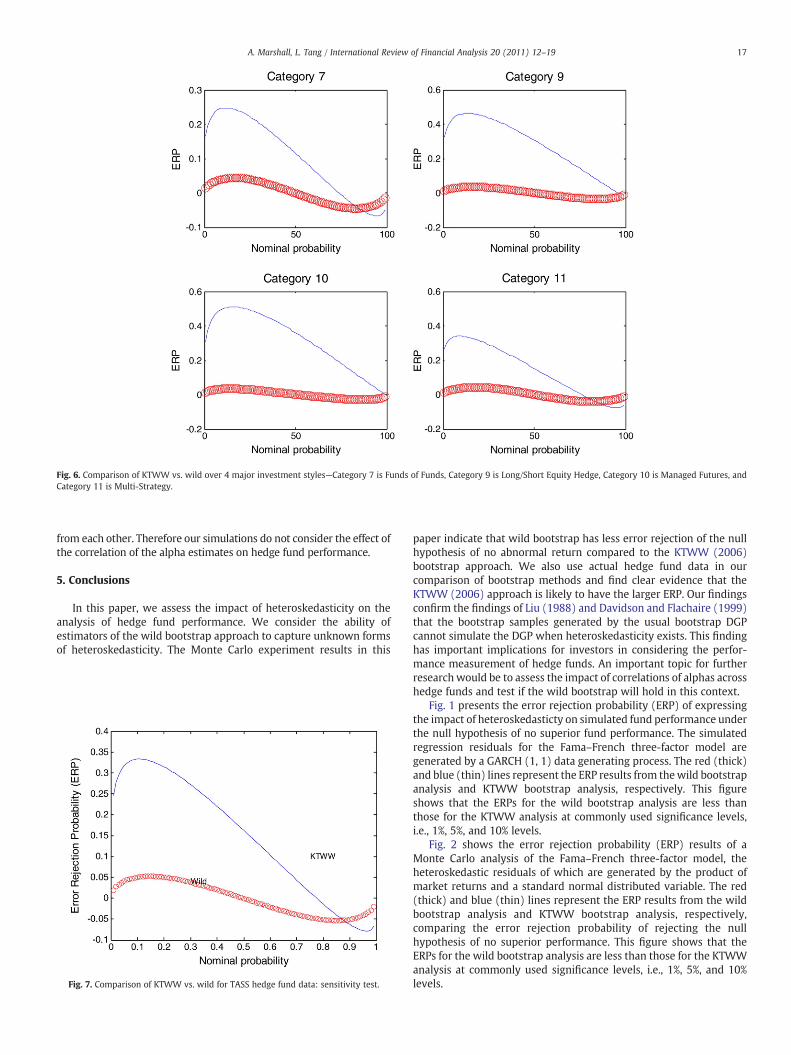
Fig. 6. Comparison of KTWW vs. wild over 4 major investment styles—Category 7 is Funds of Funds, Category 9 is Long/Short Equity Hedge, Category 10 is Managed Futures, andCategory 11 is Multi-Strategy.

17A. Marshall, L. Tang / International Review of Financial Analysis 20 (2011) 12–19

from each other. Therefore our simulations do not consider the effect ofthe correlation of the alpha estimates on hedge fund performance.

5. Conclusions

In this paper, we assess the impact of heteroskedasticity on theanalysis of hedge fund performance. We consider the ability ofestimators of the wild bootstrap approach to capture unknown formsof heteroskedasticity. The Monte Carlo experiment results in this

Fig. 7. Comparison of KTWW vs. wild for TASS hedge fund data: sensitivity test.

paper indicate that wild bootstrap has less error rejection of the nullhypothesis of no abnormal return compared to the KTWW (2006)bootstrap approach. We also use actual hedge fund data in ourcomparison of bootstrap methods and find clear evidence that theKTWW (2006) approach is likely to have the larger ERP. Our findingsconfirm the findings of Liu (1988) and Davidson and Flachaire (1999)that the bootstrap samples generated by the usual bootstrap DGPcannot simulate the DGP when heteroskedasticity exists. This findinghas important implications for investors in considering the perfor-mance measurement of hedge funds. An important topic for furtherresearch would be to assess the impact of correlations of alphas acrosshedge funds and test if the wild bootstrap will hold in this context.

Fig. 1 presents the error rejection probability (ERP) of expressingthe impact of heteroskedasticty on simulated fund performance underthe null hypothesis of no superior fund performance. The simulatedregression residuals for the Fama–French three-factor model aregenerated by a GARCH (1, 1) data generating process. The red (thick)and blue (thin) lines represent the ERP results from thewild bootstrapanalysis and KTWW bootstrap analysis, respectively. This figureshows that the ERPs for the wild bootstrap analysis are less thanthose for the KTWW analysis at commonly used significance levels,i.e., 1%, 5%, and 10% levels.

Fig. 2 shows the error rejection probability (ERP) results of aMonte Carlo analysis of the Fama–French three-factor model, theheteroskedastic residuals of which are generated by the product ofmarket returns and a standard normal distributed variable. The red(thick) and blue (thin) lines represent the ERP results from the wildbootstrap analysis and KTWW bootstrap analysis, respectively,comparing the error rejection probability of rejecting the nullhypothesis of no superior performance. This figure shows that theERPs for the wild bootstrap analysis are less than those for the KTWWanalysis at commonly used significance levels, i.e., 1%, 5%, and 10%levels.

Hedge fund investment style

Investment style Category based on LipperTASS hedge fund database

Frequency (%)

Convertible arbitrage Category 1 1.14Dedicated short bias Category 2 0.15Emerging markets Category 3 5.19Equity market neutral Category 4 2.54Event driven Category 5 4.60Fixed income arbitrage Category 6 1.47Fund of funds Category 7 45.1Global macro Category 8 2.69Long/short equity hedge Category 9 21.2Managed futures Category 10 5.70Multi-strategy Category 11 5.56Options strategy Category 12 0.29Other Category 13 4.42

18 A. Marshall, L. Tang / International Review of Financial Analysis 20 (2011) 12–19

Fig. 3 shows the error rejection probability (ERP) results of a MonteCarlo analysis of the Fama–French three-factor model, the hetero-skedastic residuals of which are generated by the product of marketreturns and a t-distribution with 3 degrees of freedom variable. The red(thick) and blue (thin) lines represent the ERP results from the wildbootstrap analysis and KTWW bootstrap analysis, respectively, com-paring the error rejection probability of rejecting the null hypothesis ofno superior performance. This figure shows that the ERPs for the wildbootstrap analysis are less than those for the KTWW analysis atcommonly used significance levels, i.e., 1%, 5%, and 10% levels.

Fig. 4 shows the error rejection probability (ERP) results for oursample from the Lipper TASS hedge fund database, comparing thewild bootstrap analysis and the KTWW bootstrap analysis under thenull hypothesis of no superior fund performance. We use monthlynet-of-returns of live and dead hedge fund, from January 1990 to June2009. We apply the Fama–French unconditional three-factor bench-mark model to measure fund manager performance. The red (thick)and blue (thin) lines represent the ERP results from thewild bootstrapanalysis and KTWW bootstrap analysis, respectively. Consistent withthe Monte Carlo simulation results, this figure shows that the ERPs forthe wild bootstrap analysis are less than those for the KTWW analysisat commonly used significance levels, i.e., 1%, 5%, and 10% levels,suggesting wild bootstrap analysis is well suited with the situationwhere the error terms of the regression have unknown form ofvariance structure.

Fig. 5 shows the error rejection probability (ERP) results for oursample from the Lipper TASS hedge fund database, comparing thewild bootstrap analysis and the KTWW bootstrap analysis overdifferent performance (alpha) percentiles under the parametricstatistical measurement. We use monthly net-of-returns of live anddead hedge fund, from January 1990 to June 2009. The red curverepresents the ERP results of KTWW bootstrap approach, while theblue curve represents the ERP results of wild bootstrap approach. This3-dimensional figure shows that the ERPs for the wild bootstrapanalysis are less than those for the KTWW analysis over all differentperformance (alpha) percentiles at commonly used significancelevels, i.e., 1%, 5%, and 10% levels, suggesting wild bootstrap analysisis well suited with the situation where the error terms of theregression have unknown form of variance structure.

Fig. 6 shows the error rejection probability (ERP) results for oursample from the Lipper TASS hedge fund database, comparing the wildbootstrap analysis and the KTWW bootstrap analysis over selected fourmajor investment styles under the parametric statistical measurement.We use monthly net-of-returns of live and dead hedge fund, fromJanuary 1990 to June 2009. The red and blue lines represent the ERPresults from the wild bootstrap analysis and KTWW bootstrap analysis,respectively. Consistent with the Monte Carlo simulation results, thisfigure shows that the ERPs for the wild bootstrap analysis are less thanthose for the KTWW analysis at commonly used significance levels, i.e.,1%, 5%, and 10% levels, suggesting wild bootstrap analysis is well suitedwith different investment styles.

Fig. 7 shows the error rejection probability (ERP) results for oursample from the Lipper TASS hedge fund database, comparing thewild bootstrap analysis and the KTWW bootstrap analysis under thenull hypothesis of no superior fund performance. We use monthlynet-of-returns of live and dead hedge fund, from January 1990 to June2009. We augment the Fama–French unconditional three-factorbenchmark model by adding 3 control factors to measure fundmanager performance. The red (thick) and blue (thin) lines representthe ERP results from the wild bootstrap analysis and KTWWbootstrapanalysis, respectively. Consistent with the results of Fig. 4, this figureshows that the ERPs for the wild bootstrap analysis are less than thosefor the KTWW analysis at commonly used significance levels, i.e., 1%,5%, and 10% levels, suggesting wild bootstrap analysis is well suitedwith the situation where the error terms of the regression haveunknown form of variance structure.

Appendix A

This table shows the distribution of hedge funds across TASS stylecategories from January 1990 to June 2009. We only include hedgefunds which have more than five years of data and have reported allnecessary data without a break over their lifetime.

References

Ackermann, C., McEnally, R., & Ravenscraft, D. (1999). The performance of hedge funds:Risk, return, and incentives. Journal of Finance, 54, 833−874.

Agarwal, V., Bakshi, G., and Huij, J. (2008). Dynamic investment opportunities and thecross-section of hedge fund returns: Implications of higher-moment risks forperformance. Working Paper No. RHS-06-066. University of Maryland.

Agarwal, V., & Naik, N. (2004). Risks and portfolio decisions involving hedge funds.Review of Financial Studies, 17, 63−98.

Amin, G., & Kat, H. (2003). Hedge fund performance 1990–2000: Do the moneymachine really add value? Journal of Financial and Quantitative Analysis, 38,251−274.

Berk, J., & Green, R. (2004). Mutual fund flows and performance in rational markets.Journal of Political Economy, 112, 1269−1295.

Blake, D., Lehmann, B., & Timmerman, A. (1999). Asset allocation dynamics and pensionfund performance. Journal of Business, 72, 429.

Bollerslev, T. (1986). Generalized autoregressive conditional heteroskedasticity. Journalof Econometrics, 31, 307−327.

Boyson, N. (2008). Hedge fund performance persistence: A new approach. FinancialAnalysts Journal, 64, 27−43.

Brooks, C., & Kat, H. (2002). The statistical properties of hedge fund index returns andtheir implications for investors. The Journal of Alternative Investments, 5, 26−44.

Brown, S., Goetzman, J., & Roger, G. (1992). Offshore hedge funds: Survival andperformance, 1989–1995. Journal of Business, 72, 91−117.

Brown, S., & Goetzman, W. (1995). Performance persistence. Journal of Finance, 50,679−698.

Carhart, M. (1997). On persistence in mutual fund performance. Journal of Finance, 52,57−82.

Chen, C., & Keown, A. (1981). Risk decomposition and portfolio diversification whenbeta is nonstationary: A note. Journal of Finance, 36, 941−947.

Cribari-Neto, F., & Zarkos, S. G. (1999). Bootstrap methods for heteroskedasticregression models: Evidence on estimation and testing. Econometric Reviews, 18,211−228.

Davidson, R., & Flachaire, E. (1999). The wild bootstrap, Tamed at last. Journal ofEconometrics, 146(1), 162−169.

Davidson, R., & MacKinnon, J. (2004). Econometric theory and methods. New York:Oxford University Press.

Fama, E., & French, K. (1993). Common risk factors in the returns on bonds and stocks.Journal of Financial Economics, 33, 3−53.

Fama, E., & French, K. (2010). Luck versus skill in the cross section of mutual fundreturns. Journal of Finance, 65, 1915−1947.

Ferson, W., & Schadt, R. (1996). Measuring fund strategy and performance in changingeconomic conditions. Journal of Finance, 51, 425−461.

Flachaire, E. (2005). Bootstrapping heteroskedastic regression models: Wild bootstrapvs. pairs bootstrap. Computational Statistics and Data Analysis, 49, 361−376.

Friend, I., & Blume, M. (1970). Measurement of portfolio performance underuncertainty. The American Economic Review, 60, 561−575.

Fung, W., & Hsieh, D. (1997). Empirical characteristics of dynamic trading strategies:The case of hedge funds. Review of Financial Studies, 10, 275−302.

Fung, W., & Hsieh, D. (2004). Hedge fund bench marks: A risk based approach. FinancialAnalyst Journal, 60, 65−80.

Fung, W., & Hsieh, D. (2009). Measurement biases in hedge fund performance data: Anupdate. Financial Analysts Journal, 65, 36−38.

19A. Marshall, L. Tang / International Review of Financial Analysis 20 (2011) 12–19

Goncalves, S., & Killian, L. (2004). Bootstrapping autoregressoins with heteroskedas-ticity of unknown form. Journal of Econometrics, 123, 89−120.

Grinblatt, M., Titman, S., & Wermers, R. (1995). Momentum investment strategies,portfolio performance, and herding: A study of mutual fund behavior. The AmericanEconomic Review, 85, 1088−1105.

Hall, P. (1992). The bootstrap and edgeworth expansion. Springer Series in Statistics.Springer Verlag.

Hansen, B. (1999). The grid bootstrap and the autoregressive models. The Review ofEconomics and Statistics, 81, 594−607.

Hinkley, D. (1977). Jackknifing in unbalanced situations. Technometrics, 19, 285−292.Horowitz, B. (1997). Bootstrap methods in econometrics: Theory and numerical

performance. In D. Kreps, & K.Wallis (Eds.), Advances in Economic and Econometrics.Seven World Congress, Vol. III. (pp. 188−222).

Jensen, M. (1968). Problems in selection of security portfolios: The importance ofmutual funds in the period 1945–1964. Journal of Finance, 32, 389−416.

Judge, G., Hill, R., Griffiths, W., Lutkepohl, H., & Lee, T. (1985). The theory and practice ofeconometrics. New York: John Wiley & Sons.

Kosowski, R., Naik, N., & Teo, M. (2007). Do hedge funds deliver alpha? A Bayesian andbootstrap analysis. Journal of Financial Economics, 84, 229−264.

Kosowski, R., Timmermann, A., Wermers, R., & White, H. (2006). Can mutual fund starsreally pick stocks? New evidence from a bootstrap analysis. Journal of Finance, 61,2551−2596.

Liang, B. (2000). Hedge funds: The living and the dead. Journal of Financial andQuantitative Analysis, 35, 309−326.

Liu, R. (1988). Bootstrap procedure under some non-I.I.D. models. Annals of Statistics,16, 1696−1708.

Mammen, E. (1993). Bootstrap and wild bootstrap for high dimensional linear models.Annals of Statistics, 21, 255−285.

Newey, W., & West, K. (1987). A positive semi-definite, heteroskedasticity and auto-correlated covariance matrix. Econometrica, 55, 703−708.

Sharpe, W. (1966). Mutual fund performance. Journal of Business, 39, 119−138.Wermers, R. (2000). Mutual fund performance: An empirical decomposition into stock-

picking talent, style, transactions costs, and expenses. Journal of Finance, 55,1655−1695.