Embed Size (px)
Citation preview
Applied Econometrics
Applied EconometricsSecond edition
Dimitrios Asteriou and Stephen G. Hall
Applied Econometrics
HETEROSKEDASTICITY
1. What is Heteroskedasticity
2. Consequences of Heteroskedasticity
3. Detecting Heteroskedasticity
4. Resolving Heteroskedasticity
Applied Econometrics
Learning Objectives1. Understand the meaning of heteroskedasticity and
homoskedasticity through examples.
2. Understand the consequences of heteroskedasticity on OLS estimates.
3. Detect heteroskedasticity through graph inspection.
4. Detect heteroskedasticity through formal econometric tests.
5. Distinguish among the wide range of available tests for detecting heteroskedasticity.
6. Perform heteroskedasticity tests using econometric software.
7. Resolve heteroskedasticity using econometric software.
Applied Econometrics
What is Heteroskedasticity
Hetero (different or unequal) is the opposite of Homo (same or equal)…
Skedastic means spread or scatter…
Homoskedasticity = equal spread
Heteroskedasticity = unequal spread
Applied Econometrics
What is Heteroskedasticity
Assumption 5 of the CLRM states that the disturbances should have a constant (equal) variance independent of t:
Var(ut)=σ2
Therefore, having an equal variance means that the disturbances are homoskedastic.
Applied Econometrics
What is HeteroskedasticityIf the homoskedasticity assumption is
violated then
Var(ut)=σt2
Where the only difference is the subscript t, attached to the σt
2, which means that the variance can change for every different observation in the sample t=1, 2, 3, 4, …, n.
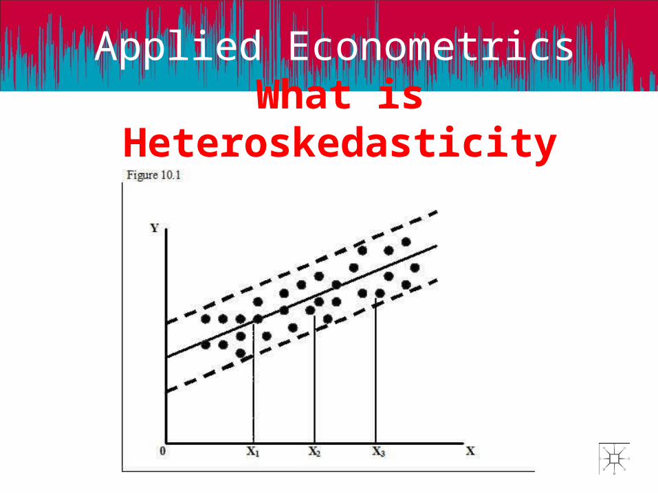
Look at the following graphs…
Applied Econometrics
What is Heteroskedasticity
Applied Econometrics
What is Heteroskedasticity
Applied Econometrics
What is Heteroskedasticity
Applied Econometrics
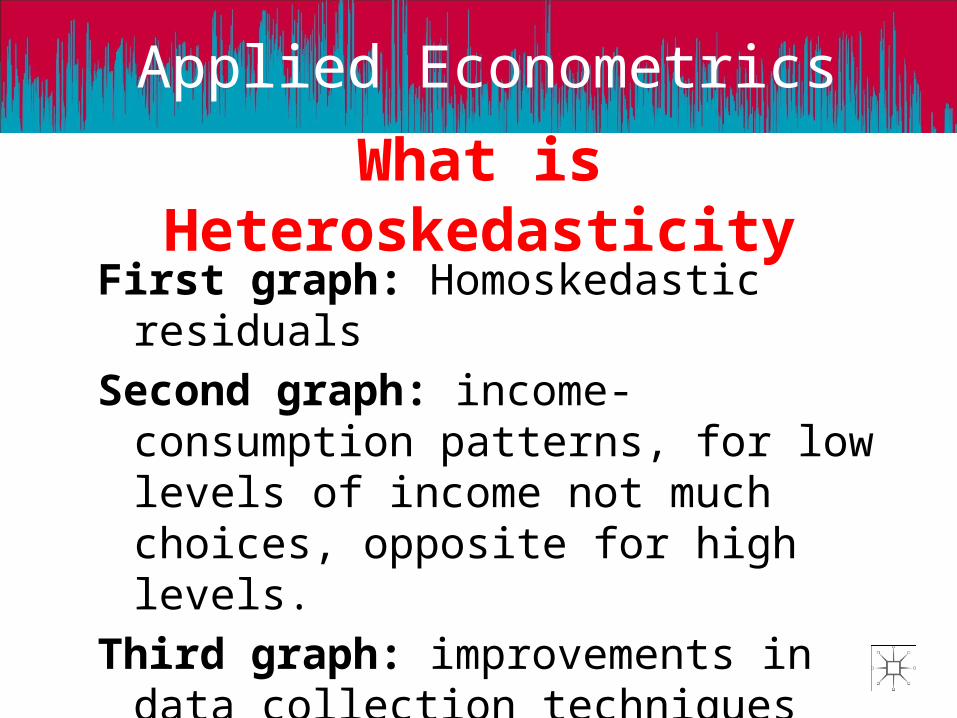
What is HeteroskedasticityFirst graph: Homoskedastic residuals
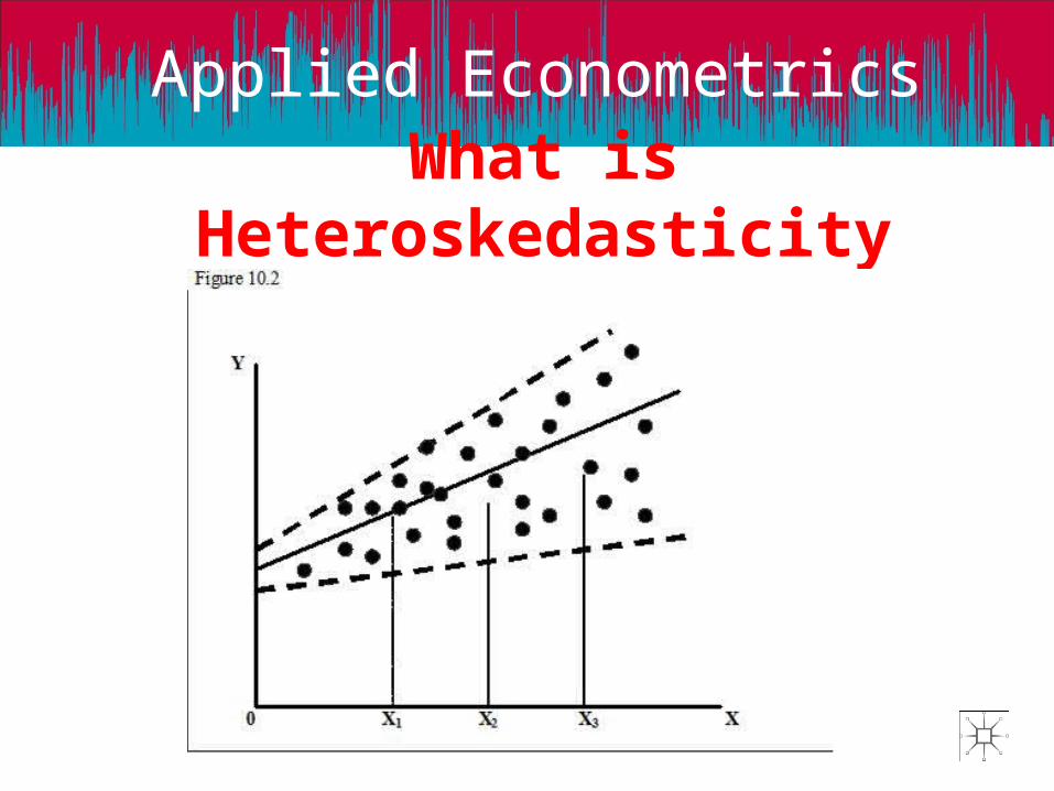
Second graph: income-consumption patterns, for low levels of income not much choices, opposite for high levels.
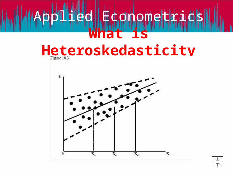
Third graph: improvements in data collection techniques (large banks) or to error learning models (experience decreases the chance of making large errors).
Applied Econometrics
Consequences of Heteroskedasticity
1. The OLS estimators are still unbiased and consistent. This is because none of the explanatory variables is correlated with the error term. So a correctly specified equation will give us values of estimated coefficient which are very close to the real parameters.
2. Affects the distribution of the estimated coefficients increasing the variances of the distributions and therefore making the OLS estimators inefficient.
3. Underestimates the variances of the estimators, leading to higher values of t and F statistics.
Applied Econometrics
Detecting HeteroskedasticityThere are two ways in general.The first is the informal way which is done through graphs
and therefore we call it the graphical method.The second is through formal tests for heteroskedasticity,
like the following ones:
1. The Breusch-Pagan LM Test2. The Glesjer LM Test3. The Harvey-Godfrey LM Test4. The Park LM Test5. The Goldfeld-Quandt Tets6. White’s Test
Applied Econometrics
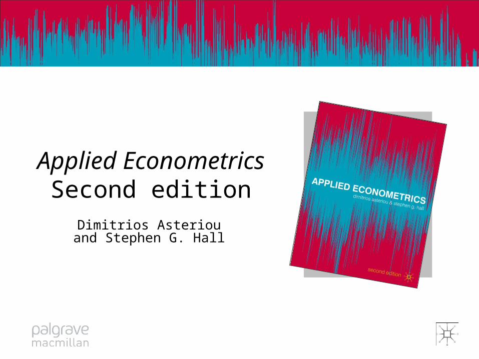
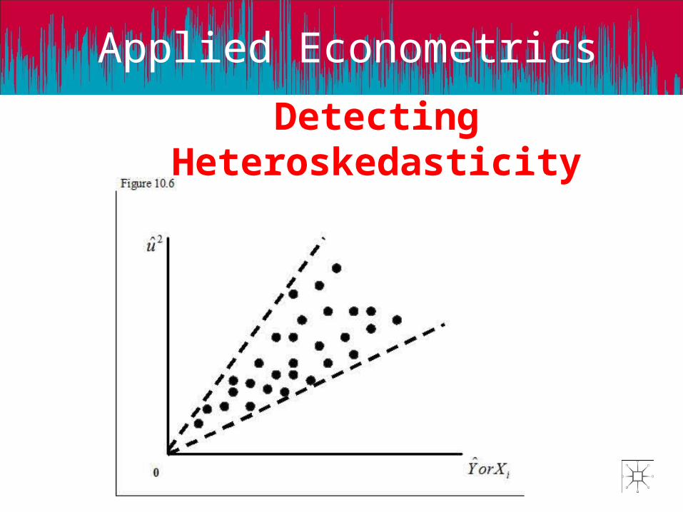
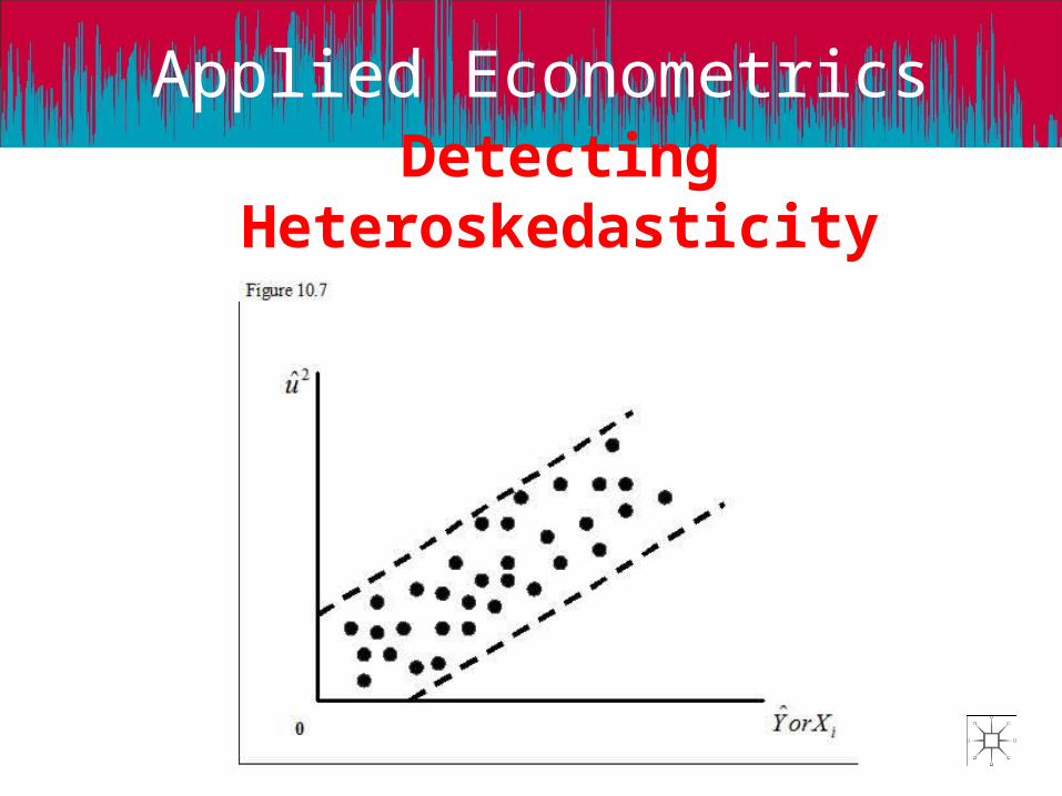
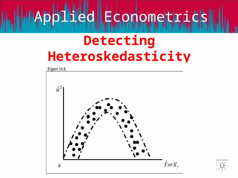
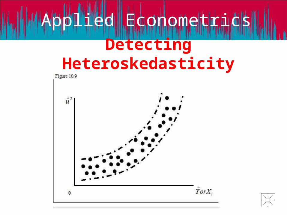
Detecting Heteroskedasticity
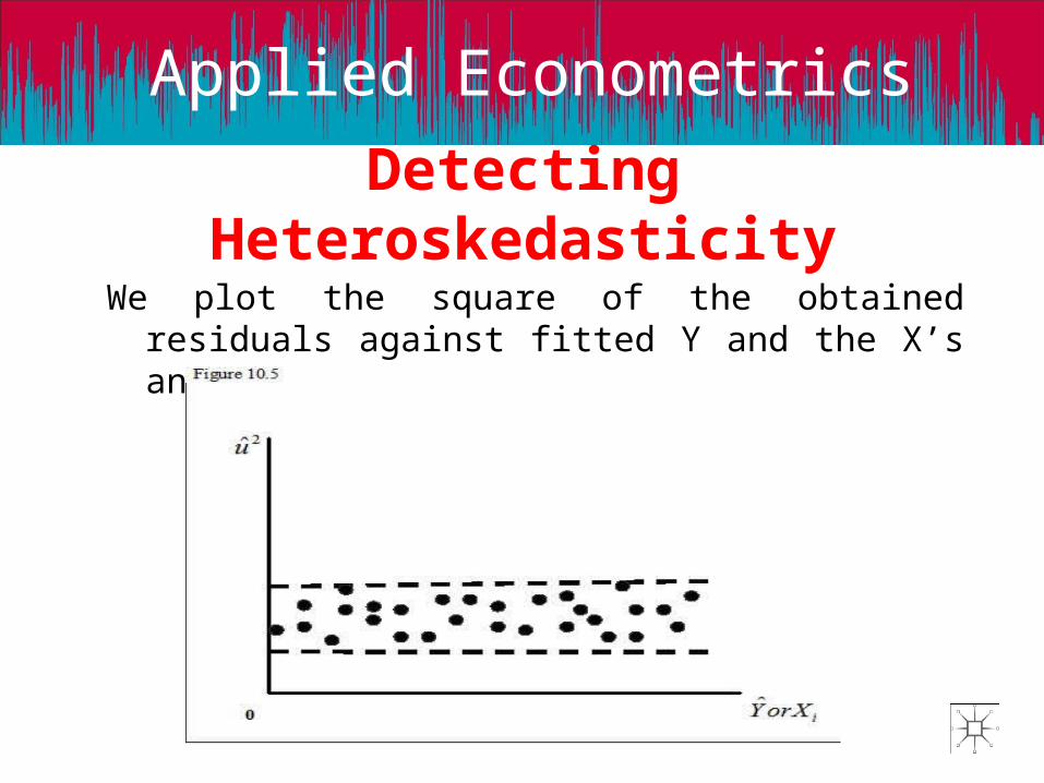
We plot the square of the obtained residuals against fitted Y and the X’s and we see the patterns.
Applied Econometrics
Detecting Heteroskedasticity
Applied Econometrics
Detecting Heteroskedasticity
Applied Econometrics
Detecting Heteroskedasticity
Applied Econometrics
Detecting Heteroskedasticity
Applied Econometrics
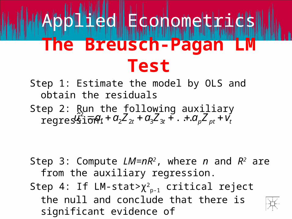
The Breusch-Pagan LM Test
Step 1: Estimate the model by OLS and obtain the residuals
Step 2: Run the following auxiliary regression:
Step 3: Compute LM=nR2, where n and R2 are from the auxiliary regression.
Step 4: If LM-stat>χ2p-1 critical reject the null and conclude
that there is significant evidence of heteroskedasticity
tptpttt vZaZaZaau ...ˆ 332212
Applied Econometrics
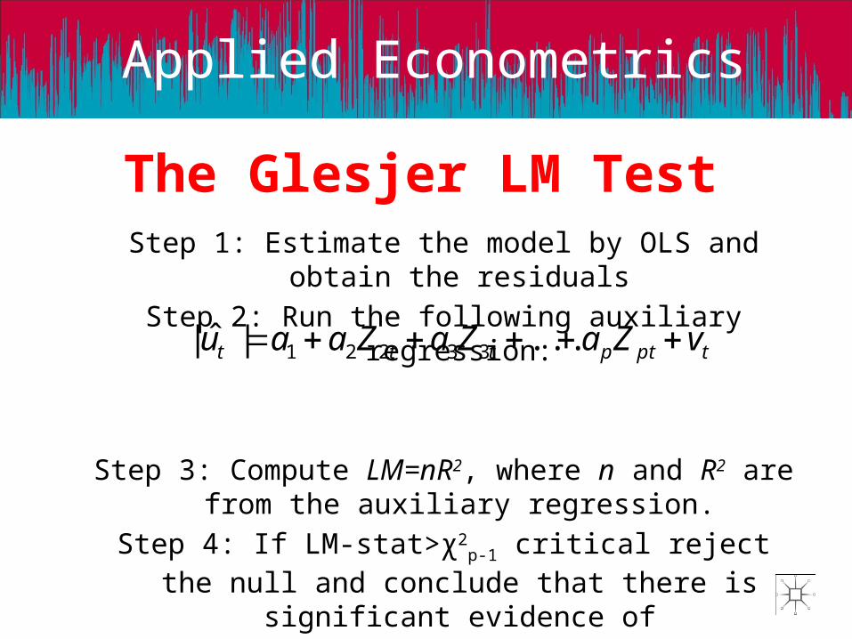
The Glesjer LM TestStep 1: Estimate the model by OLS and obtain the residuals
Step 2: Run the following auxiliary regression:
Step 3: Compute LM=nR2, where n and R2 are from the auxiliary regression.
Step 4: If LM-stat>χ2p-1 critical reject the null and conclude
that there is significant evidence of heteroskedasticity
tptpttt vZaZaZaau ...|ˆ| 33221
Applied Econometrics
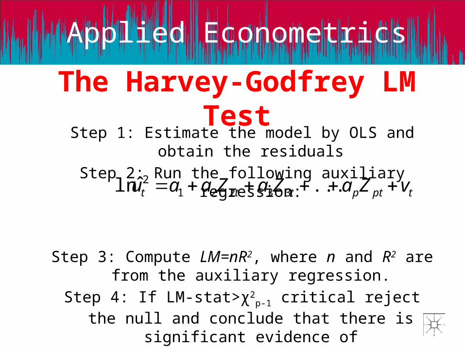
The Harvey-Godfrey LM Test Step 1: Estimate the model by OLS and obtain the residuals
Step 2: Run the following auxiliary regression:
Step 3: Compute LM=nR2, where n and R2 are from the auxiliary regression.
Step 4: If LM-stat>χ2p-1 critical reject the null and conclude
that there is significant evidence of heteroskedasticity
tptpttt vZaZaZaau ...ˆln 332212

Applied Econometrics
The Park LM TestStep 1: Estimate the model by OLS and obtain the residuals
Step 2: Run the following auxiliary regression:
Step 3: Compute LM=nR2, where n and R2 are from the auxiliary regression.
Step 4: If LM-stat>χ2p-1 critical reject the null and conclude
that there is significant evidence of heteroskedasticity
tptpttt vZaZaZaau ln...lnlnˆln 332212
Applied Econometrics
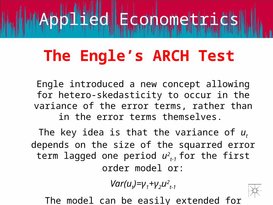
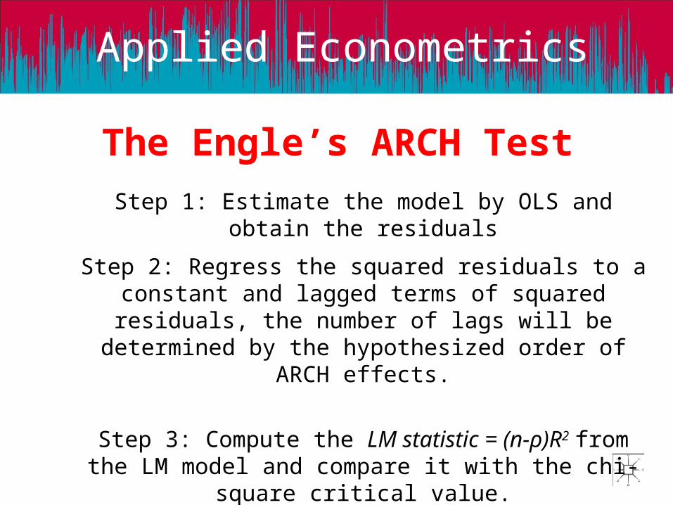
The Engle’s ARCH Test
Engle introduced a new concept allowing for hetero-skedasticity to occur in the variance of the error terms, rather
than in the error terms themselves.
The key idea is that the variance of ut depends on the size of the squarred error term lagged one period u2
t-1 for the first order model or:
Var(ut)=γ1+γ2u2t-1
The model can be easily extended for higher orders:
Var(ut)=γ1+γ2u2t-1+…+ γpu2
t-p
Applied Econometrics
The Engle’s ARCH Test
Step 1: Estimate the model by OLS and obtain the residuals
Step 2: Regress the squared residuals to a constant and lagged terms of squared residuals, the number of lags will be
determined by the hypothesized order of ARCH effects.
Step 3: Compute the LM statistic = (n-ρ)R2 from the LM model and compare it with the chi-square critical value.
Step 4: Conclude
Applied Econometrics
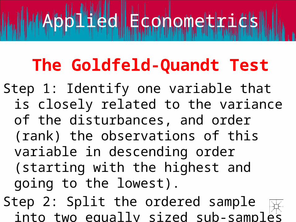
The Goldfeld-Quandt TestStep 1: Identify one variable that is closely related to
the variance of the disturbances, and order (rank) the observations of this variable in descending order (starting with the highest and going to the lowest).
Step 2: Split the ordered sample into two equally sized sub-samples by omitting c central observations, so that the two samples will contain ½(n-c) observations.
Applied Econometrics
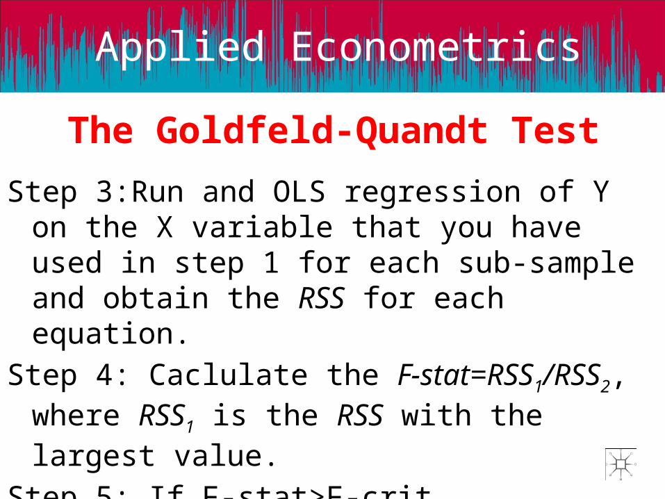
The Goldfeld-Quandt Test
Step 3:Run and OLS regression of Y on the X variable that you have used in step 1 for each sub-sample and obtain the RSS for each equation.
Step 4: Caclulate the F-stat=RSS1/RSS2, where RSS1 is the RSS with the largest value.
Step 5: If F-stat>F-crit(1/2(n-c)-l,1/2(n-c)-k) reject the null of homoskedasticity.
Applied Econometrics
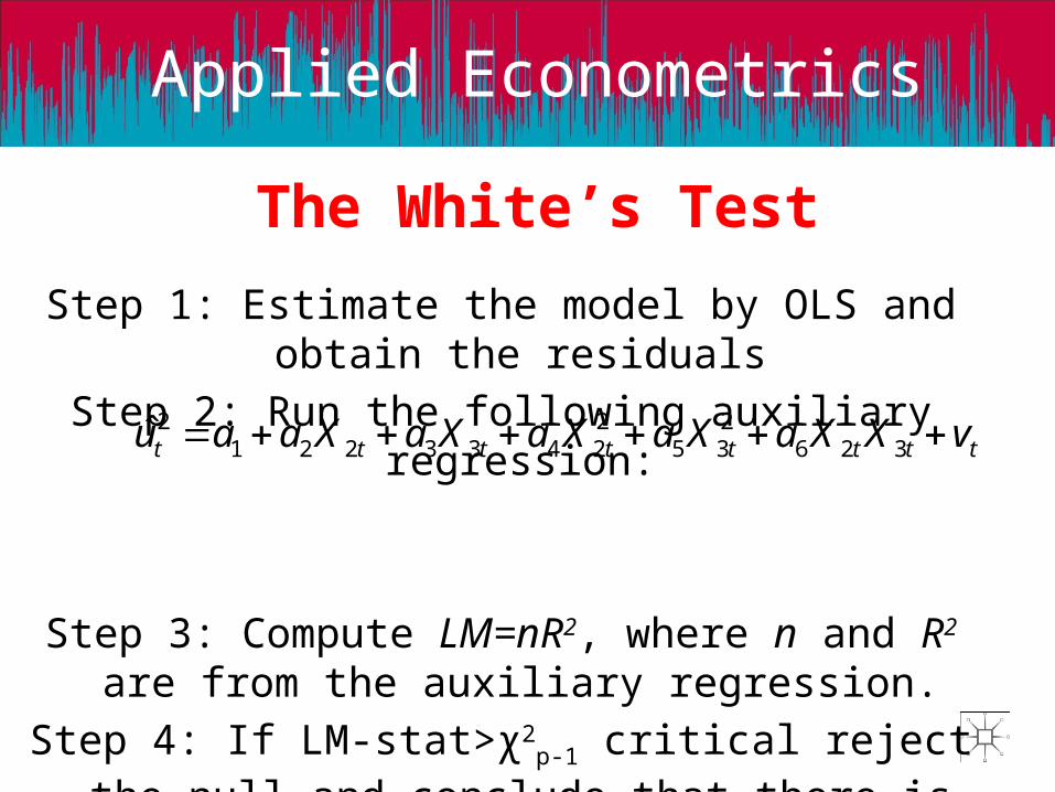
The White’s Test
Step 1: Estimate the model by OLS and obtain the residuals
Step 2: Run the following auxiliary regression:
Step 3: Compute LM=nR2, where n and R2 are from the auxiliary regression.
Step 4: If LM-stat>χ2p-1 critical reject the null and conclude
that there is significant evidence of heteroskedasticity
tttttttt vXXaXaXaXaXaau 326235
22433221
2ˆ
Applied Econometrics
Resolving Heteroskedasticity
We have three different cases:
(a) Generalized Least Squares
(b) Weighted Least Squares
(c) Heteroskedasticity-Consistent Estimation Methods
Applied Econometrics
Generalized Least Squares
Consider the model
Yt=β1+β2X2t+β3X3t+β4X4t+…+βkXkt+ut
where
Var(ut)=σt2
Applied Econometrics
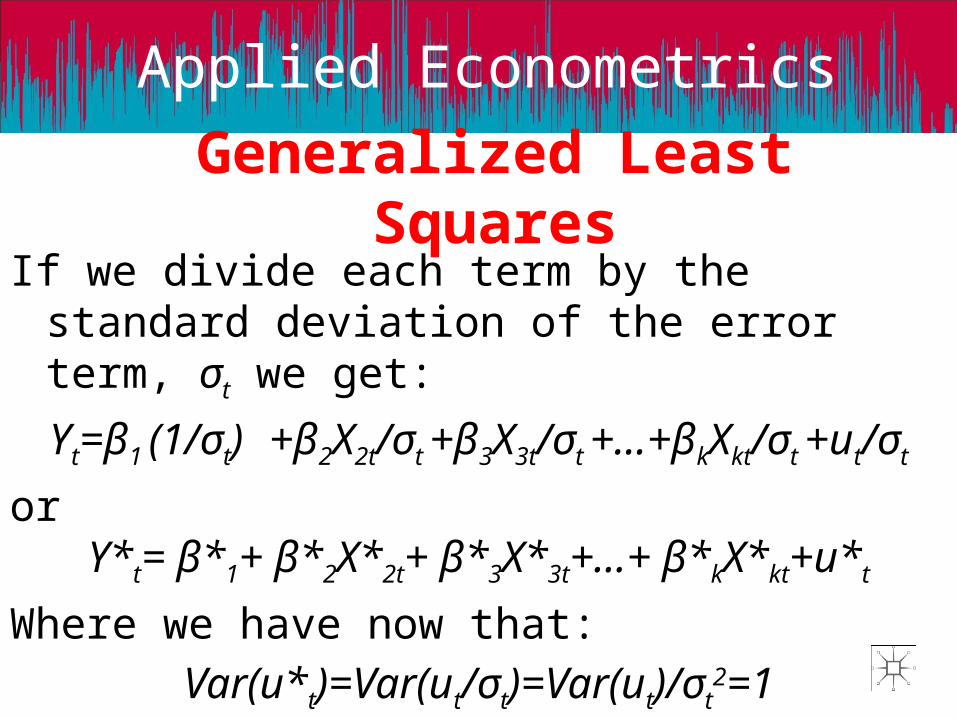
Generalized Least SquaresIf we divide each term by the standard deviation of the
error term, σt we get:
Yt=β1 (1/σt) +β2X2t/σt +β3X3t/σt +…+βkXkt/σt +ut/σt
orY*t= β*1+ β*2X*2t+ β*3X*3t+…+ β*kX*kt+u*t
Where we have now that:
Var(u*t)=Var(ut/σt)=Var(ut)/σt2=1
Applied Econometrics
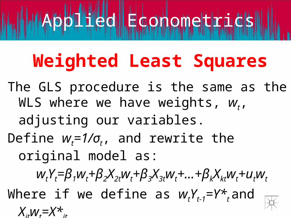
Weighted Least SquaresThe GLS procedure is the same as the WLS where
we have weights, wt, adjusting our variables.
Define wt=1/σt, and rewrite the original model as:
wtYt=β1wt+β2X2twt+β3X3twt+…+βkXktwt+utwt
Where if we define as wtYt-1=Y*t and Xitwt=X*it
we get
Y*t= β*1+ β*2X*2t+ β*3X*3t+…+ β*kX*kt+u*t