QEDQueen’s Economics Department Working Paper No. 537

Some Heteroskedasticity-Consistent Covariance MatrixEstimators with Improved Finite Sample Properties

James G. MacKinnonQueen’s University

Halbert WhiteUniversity of California San Diego

Department of EconomicsQueen’s University

94 University AvenueKingston, Ontario, Canada

K7L 3N6

4-1985

brought to you by COREView metadata, citation and similar papers at core.ac.uk

provided by Research Papers in Economics

Some Heteroskedasticity-Consistent

Covariance Matrix Estimators with

Improved Finite Sample Properties

James G. MacKinnon

Department of EconomicsQueen’s University

Kingston, Ontario, CanadaK7L 3N6

Halbert White

Department of EconomicsUniversity of California, San Diego

La Jolla, CA 92093U.S.A.

Abstract

We examine several modified versions of the heteroskedasticity-consistent covariancematrix estimator of Hinkley (1977) and White (1980). On the basis of samplingexperiments which compare the performance of quasi t statistics, we find that oneestimator, based on the jackknife, performs better in small samples than the rest. Wealso examine finite-sample properties using modified critical values based on Edge-worth approximations, as proposed by Rothenberg (1988). In addition, we comparethe power of several tests for heteroskedasticity and find that it may be wise to em-ploy the jackknife heteroskedasticity-consistent covariance matrix even in the absenceof detected heteroskedasticity.

We are very grateful to an anonymous referee for a number of very useful suggestions andcomments. An earlier version of this paper appeared as UCSD Department of EconomicsDiscussion Paper No. 82-18. The paper was later published in the Journal of Econometrics,29, 1985, 305–325, and references have been updated. Some computer funds were providedby the University of California, but most of the computing was done on an IBM 3081 atQueen’s University. MacKinnon’s research was supported, in part, by grants from the SocialSciences and Humanities Research Council of Canada.

July, 1983; revised April, 1985

1. Introduction

The linear regression model is extensively used by applied econometricians. Togetherwith its numerous generalizations, it constitutes the foundation of most empiricalwork in economics. Despite this fact, little is known about properties of inferencesmade from this model when standard assumptions are violated. In particular, classi-cal techniques require one to assume that the error terms have a constant variance.This assumption is often not very plausible. Nevertheless, a way of consistently esti-mating the variance-covariance matrix of ordinary least squares estimates in the faceof heteroskedasticity of known form is available; see Eicker (1963), Hinkley (1977),and White (1980). This heteroskedasticity-consistent covariance matrix estimatorallows one to make valid inferences provided the sample size is sufficiently large.

Unfortunately, it is not at all obvious what ‘sufficiently large’ means in practice, andit is well known that statistics with identical large sample properties can performvery differently in samples of small or modest size. In this paper, we examine someestimators which are asymptotically equivalent to the heteroskedasticity-consistentcovariance matrix estimator alluded to above, but which may be expected to havesuperior finite sample properties. Since covariance matrix estimators are most fre-quently used to construct test statistics, we focus on the behavior of quasi t statisticsconstructed using these different estimators. Using sampling experiments, we findthat all the new estimators outperform the original one, and that one of them, basedon the jackknife, consistently outperforms the other two. These experiments alsoshow that, in some circumstances, the original estimator can be highly misleading,sometimes even more misleading than the conventional OLS covariance matrix whichignores the possibility of heteroskedasticity.

We next consider an alternative approach due to Rothenberg (1988), in which theoriginal heteroskedasticity-consistent estimator is used in conjunction with modifiedcritical values based on Edgeworth approximations. This approach appears to workwell, especially when the sample is reasonably large. Finally, we consider the relatedquestion of how well alternative tests for heteroskedasticity perform in the environ-ments studied here. We find that the ‘portmanteau’ test of White (1980) generallyperforms well. However, the evidence also suggests that it may be wise to use aheteroskedasticity-consistent covariance matrix estimator even in the absence of de-tected heteroskedasticity.

The structure of the paper is as follows. In section 2, we describe the problemand the various estimators that will be examined. In sections 3 and 4, we describethe experiments to be performed and present the results of those experiments. Insection 5, we discuss the use of modified critical values based on Edgeworth approx-imations. Finally, in section 6, we examine the performance of alternative tests forheteroskedasticity.

–1–

2. Statement of the problemIn this paper, we deal exclusively with the linear regression model

y = Xβ + u, (1)

where y is an n × 1 vector of observations on a dependent variable, X is an n × kmatrix of observations on independent variables, assumed to be of full rank, and uis an n × 1 vector of observations on an error term with mean zero. The ordinaryleast squares estimator for this model is

β = (X>X)−1X>y. (2)

Inferences about β may be based on the fact that β − β has mean vector zero andcovariance matrix

(X>X)−1X>ΩX(X>X)−1, (3)

where E(uu>) = Ω.

Conventionally, it is assumed that E(uu>) = σ2In. Thus expression (3) simplifies toσ2(X>X)−1, which can be conveniently estimated as

σ2(X>X)−1, σ2 =u>un− k

, u =(In −X(X>X)−1X>)

y. (4)

If X is non-stochastic and u is normally distributed, exact inferences in finite samplescan then be based on the t or F distributions. Otherwise, (4) serves as the basis forvalid asymptotic inference.

The assumption that the errors are homoskedastic is often implausible. Instead, onemay assume that E(u2

t ) = σ2t , where σt varies in some unknown fashion over observa-

tions. A heteroskedasticity-consistent covariance matrix estimator which allows oneto estimate (3) consistently under general conditions is

(X>X)−1X>ΩX(X>X)−1, (5)

whereΩ = diag(u2

1, u22, . . . , u

2n);

see White (1980).

The estimator (5), which we shall refer to henceforth as HC, takes no account of thewell-known fact that OLS residuals tend to be ‘too small’. One simple way to modifyHC is to use a degrees of freedom correction similar to the one conventionally usedto obtain unbiased estimates of σ2. This yields the modified estimator

n

n− k(X>X)−1X>ΩX(X>X)−1, (6)

–2–

which was suggested by Hinkley (1977). We shall refer to this estimator as HC1.

The degrees of freedom adjustment in HC1 is not the only way to compensate forthe fact that the OLS residuals tend to underestimate the true errors. If there is noheteroskedasticity, it is easily seen that

E(u2t ) = (1− ktt)σ2, (7)

where ktt is the tth diagonal element of the matrix X(X>X)−1X>. Thus Horn, Horn,and Duncan (1975) suggest using

σt =u2

t

1− ktt(8)

as an ‘almost unbiased’ estimator for σt. Following their approach, we propose theestimator

(X>X)−1X>ΩX(X>X)−1, (9)

whereΩ = diag(σ2

1 , σ22 , . . . , σ2

n),

as an alternative way to estimate (3) consistently. We shall refer to this estimatoras HC2. It is immediate from (7) that HC2 will be unbiased when the ut are in facthomoskedastic. In contrast, as Hinkley (1977) points out, HC1 will only be unbiasedin the special case of a ‘balanced’ experimental design, for which ktt = k/n for all t.

All of these covariance matrix estimators are intimately related to what statisticiansrefer to as the ‘jackknife’. Efron (1982, p. 19) points out that what is essentially HCcan be obtained by the infinitesimal jackknife method. Hinkley (1977) derived HC1

as the covariance matrix of what he called the ‘weighted jackknife’ estimator, andit would have been possible to derive HC2 using a very similar argument, althoughHinkley did not in fact do so. All of this suggests that the ordinary jackknife (seeEfron, 1982) might provide another modified heteroskedasticity-consistent covariancematrix estimator, and indeed that turns out to be the case.

The basic idea of the jackknife is to recompute the estimates of a model n times,each time dropping one of the observations, and then to use the variability of therecomputed estimates as an estimate of the variability of the original estimator. Formore details, see Efron (1982). Let β(t) denote the OLS estimate of β based on allobservations except the tth. It is easily shown that

β(t) = β − (X>X)−1Xt>u∗t , (10)

where Xt denotes the tth row of X and u∗t = ut/(l − ktt). Then, from expression(3.13) of Efron (1982), the jackknife estimate of the covariance matrix of β is givenby the k × k matrix

–3–

n− 1n

n∑t=1

(β(t) − 1−

n

n∑s=1

β(s)

)(β(t) − 1−

n

n∑s=1

β(s)

)>. (11)

After considerable manipulation,1 it can be shown that (11) reduces to

n− 1n

(X>X)−1(X>Ω∗X − 1−

nX>u∗u∗>X

)(X>X)−1 (12)

where Ω∗ is an n×n diagonal matrix with diagonal elements of u∗2t and off-diagonalelements of zero, and u∗ is a vector of the u∗t . We shall refer to this covariance matrixestimator as HC3. It is evident that HC3 is asymptotically equivalent to HC, HC1,and HC2, since 1/n times the middle factor clearly converges to 1/n times X>ΩX.

As Messer and White (1984) have shown, it is easy to trick a conventional regressionpackage which is capable of IV estimation into producing HC or HC1. If the ktt canbe obtained and used to compute the σt, their technique can also be used to makea regression package produce HC2. Calculating HC3 will inevitably be a little moredifficult. Almost all the calculations can, however, be performed with a regressionpackage, since (12) can be rewritten as

n− 1n

(X>X)−1X>Ω∗X(X>X)−1 − n− 1n2

γγ>, (13)

where γ = (X>X)−1X>u∗. It is tempting to omit the factor (n− 1)/n in HC3. Theeffect of this omission will normally be very small. Moreover, experimental results(see below) suggest that this small effect would normally be in the right direction.because we did not know that when the experiments were designed, however, weretained the factor (n− 1)/n in those experiments.

Since covariance matrix estimators are usually used to compute test statistics, wefocus our experiments directly on the behavior of such test statistics. In particular,we examine the small-sample performance of quasi t statistics to test hypotheses thatparticular elements of β assume specified values. For related evidence on how wellestimators such as HC and HC1 approximate the true covariance matrix directly, seeCragg (1983) and Nicholls and Pagan (1983).

One important property of these quasi t statistics may be noted immediately. Whenthe hypothesis being tested is true, the numerator of such a statistic does not dependon β, and it is homogeneous of degree one in σ. The covariance matrices (4), (6),(9), and (12) also do not depend on β, and they are homogeneous of degree two in σ.Thus these test statistics themselves do depend on either β or σ. They only dependon the Xt and the ut, which may be normalized to have arbitrary variance. Since

1 When we wrote earlier versions of this paper, we were under the false impression thatthe jackknife covariance estimator is computationally too complicated to be worthstudying. We are extremely grateful to an anonymous referee for pointing out thatit can be expressed in the form of (12).

–4–

the exact finite sample properties of these test statistics are otherwise quite difficultto obtain analytically, we investigate these properties using sampling experiments.

3. Design of the experiments

In all of our experiments, we utilized the following model:

yt = β0 + β1X1t + β2X2t + ut, (14)

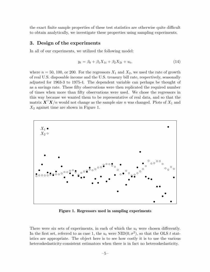
where n = 50, 100, or 200. For the regressors X1 and X2, we used the rate of growthof real U.S. disposable income and the U.S. treasury bill rate, respectively, seasonallyadjusted for 1963-3 to 1975-4. The dependent variable can perhaps be thought ofas a savings rate. These fifty observations were then replicated the required numberof times when more than fifty observations were used. We chose the regressors inthis way because we wanted them to be representative of real data, and so that thematrix X>X/n would not change as the sample size n was changed. Plots of X1 andX2 against time are shown in Figure 1.

•••

•

• • ••

•

•

••• ••• • •

••

••••

•

• •

•

•

•

•

•

•• • •

•

•

•

• • •

•

• •

• •

•

•

•

•X1

X2

Figure 1. Regressors used in sampling experiments

There were six sets of experiments, in each of which the ut were chosen differently.In the first set, referred to as case 1, the ut were NID(0, σ2), so that the OLS t stat-istics are appropriate. The object here is to see how costly it is to use the variousheteroskedasticity-consistent estimators when there is in fact no heteroskedasticity.

–5–

In the next two sets of experiments (cases 2 and 3), the variance of ut changedabruptly, as if due to some sort of structural change. The errors ut were chosen asN(0, σ2) for t = 1, . . . , 25, t = 51, . . . , 75, t = 101, . . . , 125, and t = 151, . . . , 175, andas N(0, α2σ2) for the remaining observations. The structural change parameter αwas chosen to be 2 in case 2 and 4 in case 3. Notice that the pattern of structuralchange we used is equivalent to replicating the first 25 observations as many times asnecessary (1, 2, or 4, depending on whether n = 50, 100, or 200), with the ut havingvariance σ2, and replicating the second 25 observations as many times as necessary,with the ut having variance α2σ2. This pattern was chosen so that increasing thesample size from 50 to 100 or 200 would not change the relationship between the ut

and the regressors.

In the final three sets of experiments (cases 4, 5 and 6), the variance of ut varied be-cause the βj varied randomly. Specifically, the model (14) was modified by assumingthat

βj = βj + vjt, vjt ∼ N(0, ω2j ), j = 0, 1, 2. (15)

Together with (14), the random coefficient specification (15) implies that

yt = β0 + β1X1t + β2X2t + ut + v0t + v1tX1t + v2tX2t. (16)

Assuming that ut and the vjt are independent of each other, the variance of the errorterm in (16) is

σ2 + ω20 + X2

1tω21 + X2

2tω22 = σ2

0(1 + X21tγ

21 + X2

2tγ22). (17)

Without loss of generality (since the statistics we will be studying are independentof β) we normalized X1t and X2t so that

∑Xit = 1 for i = 1, 2. Then, for case 4,

we chose γ1 = 1, γ2 = 1, for case 5 we chose γ1 = 3, γ2 = 1, and for case 6 we choseγ1 = 1, γ2 = 3.

Each experiment involved 2000 replications, and there were eighteen experiments inall (six cases for each of n = 50, n = 100, and n = 200).2 For each of the βi,we calculated four test statistics of the hypothesis that βi equals its value. Thesestatistics, denoted OLS, HC1, HC2, and HC3, utilize the covariance matrices afterwhich they are named. In addition, we calculated a control variate which utilizes thetrue covariance matrix (3) and is thus exactly N(0, 1).

For each experiment, we calculated the sample mean, standard deviation, skewness,and kurtosis (over the 2000 replications) of each of these test statistics. There wasnothing in the experimental results to suggest that any of them had a non-zeromean, or that their distributions were not symmetric. In the tables, therefore, weonly report the standard deviation (under ‘S.D.’) and the kurtosis (under ‘Kurt.’),which should be one and three, respectively, if the test statistic in question is N(0, 1).

2 In fact, we conducted six additional experiments in which n = 150, but the resultswere predictable given those for n = 100 and n = 200 and are therefore not reported.

–6–

If the standard deviation were in fact unity, the sample standard deviation would,assuming normality, have a variance of 1/4000. The number reported under ‘Kurt.’is a standard test statistic for kurtosis, namely, the estimated fourth moment aboutthe mean, divided by the square of the estimated second moment.

Although the moments of the sample distributions of the test statistics are of interest,they do not directly tell us how often we will be led to make invalid inferences byusing test statistics whose distributions differ from N(0, 1). It is more interesting toask what proportion of the time each of the test statistics exceeds certain criticalvalues. The critical values we chose were the 5% and 1% levels; absolute criticalvalues for the standard normal at these levels are 1.960 and 2.576, respectively.

The obvious way to estimate these rejection frequencies is to use the estimatorq = R/N , where R is the observed number of rejections and N is the number ofreplications (here 2000). A consistent estimate of the variance of this estimator isq(1 − q)/N . Since all of the test statistics have the same numerator as the controlvariate, they should all be highly correlated with it, and it should therefore be pos-sible to obtain more accurate estimates than q. Davidson and MacKinnon (1981)have proposed a simple technique for doing so, which we utilize here. If the con-trol variate has exceeded its critical value more than the expected number of times,the estimated rejection frequency for the statistic in question will be reduced by anamount that depends on how closely it and the control variate are correlated; thereverse will be true if the control variate has exceeded its critical value less than theexpected number of times. The variance of the resulting estimate will depend on theamount of correlation between the control variate and the other statistic, and it willnever exceed q(1− q)/N , asymptotically. For details, see Davidson and MacKinnon(1981).

The fact that we estimated rejection frequencies in this way should be borne inmind when reading the tables. The same estimated rejection frequency may havequite different standard errors in different cases, because the correlation between thecontrol variate and the test statistic may be different. This means that the gain fromutilizing this technique varies from case to case. In some cases, the standard errorsreported in the tables are more than sixty percent below what they would have beenif q had been used, equivalent to using 12,000 or more replications; in others, thestandard errors are only about twenty percent lower, equivalent to using less than3000 replications. These are asymptotic standard errors, but the very large numberof replications should endure their validity.

4. Results of the experiments

The results of twelve of the eighteen experiments just discussed are presented intables 1 through 4. Cases 2 and 4 are omitted to save space; the results for case 2were similar to those for case 3, but not as pronounced, while the results for case 4were reasonably similar to those for cases 5 and 6. An asterisk indicates that thequantity in question differs significantly at the one per cent level from what it should

–7–

be if the test statistic were really N(0, 1). The numbers under ‘C.V.’ are the standarddeviation and kurtosis of the control variate. The tables largely speak for themselves,but we will discuss a few points of interest.

The most obvious result in tables 1 through 4 is that almost all the quasi t statisticshave standard deviations greater than unity, so that rejection frequencies of testsbased on them almost always exceed the nominal size of the tests. As one wouldexpect, these standard deviations tend to decline as the sample size increases. Theyalso vary systematically with the coefficient being estimated, the quasi t statisticsfor β1 tending to have much larger variances than those for β0 or β2. The pattern ofheteroskedasticity has a major impact on the distributions of the quasi t statistics.They tend to be closest to their asymptotic N(0, 1) distribution when there is noheteroskedasticity, in table 1.

In every single case, the standard deviation of the quasi t statistic based on HC1

exceeded that for HC2, which in turn exceeded that for HC3. Since there was certainlyno tendency for HC3 to have too small a variance, this implies that HC3 is thecovariance matrix estimator of choice. The difference between HC1 and HC3 is oftenstriking, and the difference between HC and HC3 would, of course, be even morestriking. From table 1, it is clear that using HC or HC1 when there is in fact noheteroskedasticity and the sample size is small could easily lead to serious errors ofinference, while using HC3 is almost as reliable as using OLS.

Even HC3 did not always perform well when the sample size was small and therewas substantial heteroskedasticity. Its worst performance was in case 5 (table 3) forβ1 when n = 50. The standard deviation of the HC3 t statistic is 1.177 here, andit would incorrectly reject the null hypothesis 3.1% of the time at the nominal 1%level. But although HC3 performs poorly here, it performs much better than itscompetitors, since HC2 would reject the null 4.7% of the time, HC1 would reject it6.8% of the time, and the usual OLS t statistic would reject it 27.2% of the time.

Thus, subject to the usual qualifications about results of sampling experiments, thosein tables 1 to 4 suggest the following conclusions:

1. Among the heteroskedasticity-consistent estimators, HC3 is clearly the procedureof choice.

2. The usual OLS covariance estimator can be very seriously misleading in thepresence of heteroskedasticity. When it is, HC3 is also likely to be misleading ifthe sample size is small, but much less so than OLS.

3. When there is no heteroskedasticity, all the HC estimators are less reliable thanOLS, but HC3 does not seem to be much less reliable.

5. An alternative approach

What we have done so far is to modify the heteroskedasticity-consistent covariancematrix estimator so as to obtain test statistics whose finite sample distributions are

–8–

closer to their asymptotic ones. This is not the only approach to making more ac-curate inferences in finite samples. An alternative approach, which is theoreticallyappealing but technically demanding, would be to use the original test statistic basedon HC in conjunction with size-corrected critical values. The latter may be obtainedby the use of Edgeworth expansions, in this case second-order asymptotic approxi-mations to the distribution of the test statistic.

In a recent paper, Rothenberg (1988) has applied this technique to exactly the prob-lem that interests us in this paper. His fundamental result is that

t′α = tα

(1 +

(c1(1 + t2α) + c2(1− t2α) + c3

)/2n

), (18)

where tα is a level α critical value for the normal distribution and t′α is an adjustedlevel α critical value. The parameters c1, c2, and c3 are constants which dependin a complicated way on the regressors, the pattern of heteroskedasticity, and thecoefficient (or linear combination of coefficients) for which the test is to be conducted.In practice, the parameters c1 through c3 will have to be estimated using the leastsquares residuals, since the pattern of heteroskedasticity is unknown.

We conducted a number of experiments to see how this approach of using HC withadjusted critical values compares with the much simpler approach of using HC3

with the usual asymptotic critical values. We looked only at cases 2 and 4, theones which were not reported in tables 1 to 4. Case 2 was chosen because theheteroskedasticity was relatively mild in that case, and case 4 was chosen because itwas representative of all the random coefficient cases. Results for both these cases forsamples of size 50, 100, 200, and 400 are shown in table 5, which tabulates rejectionfrequencies for tests which are nominally at the 5% and 1% levels. ‘Edge-E’ showsthe rejection frequencies when c1, c2, and c3 are estimated from the data, as theywould have to be in practice, while ‘Edge-T’ shows the rejection frequencies when thetrue values of those parameters are used. All results are based on 10,000 replications,so experimental error should be very small.3

The results for Edge-T show that Rothenberg’s Edgeworth expansions are generallyquite good, and they become very good indeed as the sample size gets past 100. Ifanything, the corrected critical values tend to be too conservative. Unfortunately,these good results usually do not carry over to Edge-E, for which the correct criticalvalues are almost always not conservative enough. When the sample size is 50, HC3

always yields more accurate inferences than Edge-E, and that is usually the case forn = 100 as well. For n = 200 and n = 400, however, HC3 no longer outperformsEdge-E overall, although both perform very well. As one might expect from thenature of Edgeworth approximations, Edge-E typically performs less well at the 1%

3 We used 10,000 replications here instead of 2000 because early results showed thatHC3 and Edge-E performed similarly for samples of medium size, and we wanted tominimize experimental error. Results are based on ten sets of 1000 replications.

–9–

level than at the 5% level. Except for a very few cases at the 1% level with n = 50,Edge-E does always outperform HC.

These results suggest that Edgeworth expansions for t statistics based on HC are valu-able, but they may be more useful as a theoretical tool than as a practical method toobtain corrected critical values. This may however be too pessimistic. In principle,Rothenberg’s technique could be applied to HC1, HC2, or HC3 instead of to HC, andit is quite possible that this would produce improved results. The approach couldalso be modified by the use of alternative asymptotic expansions, by improved meth-ods for estimating the parameters c1, c2, and c3, or by more sophisticated methodsfor choosing a critical value, not necessarily equal to t′α, but making use of the infor-mation that t′α conveys. Thus future research may well make Edgeworth expansionslook more attractive than they do at present.

6. Tests for heteroskedasticityUsing the heteroskedasticity-consistent covariance matrix estimator as a startingpoint, White (1980) proposed a test for heteroskedasticity of unknown form. In thecase of our model (14), the White test may be carried out by regressing the squaredOLS residuals u2

t on a constant, X1, X2, X21 , X2

2 , and X1X2. The test statistic is ntimes the R2 from this regression, and it is asymptotically distributed as chi-squaredwith (in this case) 5 degrees of freedom. In the tables, this test will be referred toas HT.

In view of the success of HC2 and HC3, it is natural to wonder whether modifiedversions of the White test might perform better than the original. In the case ofHC3, it is not obvious how one should modify the test. However, in the case ofHC2, it is straightforward to modify it by using σ2

t instead of u2t as the regressand.

Unfortunately, this modified version of HT turned out to have poorer small-sampleproperties under the null than the original, and we therefore dropped it from ourexperiments.

Lagrange Multiplier tests for heteroskedasticity have recently become very popular.In the case of the random coefficient model described in section 3, a particularlysimple form of the LM test may be computed by regressing u2

t on a constant, X21 ,

and X22 . The test statistic is then n times the R2 from this regression, and it is

asymptotically distributed as chi-squared with (in this case) 2 degrees of freedom.For details, see Koenker (1981) and Breusch and Pagan (1979). A similar test maybe constructed to test against a structural change in variance. In this case, u2

t isregressed on a constant and on a dummy variable equal to 0 half the time and to 1the other half; the test has one degree of freedom. These tests will be referred to asLM1 and LM2, respectively.

Over the years, numerous ad hoc tests for heteroskedasticity have been proposed.Among the most popular of these is the F test suggested by Goldfeld and Quandt(1965). The data are ordered by time or by one of the regressors, separate regressionsare performed on the first and last thirds of the data (leaving out a third in the

–10–

middle), and the ratio of the sums of squared residuals is then formed. Under thenull, this ratio is distributed as F with both numerator and denominator degrees offreedom equal to n/3 − k. The test has the advantage of being exact, but it mayhave little power if the actual heteroskedasticity is not closely related to time or toone of the regressors. We calculated three tests of this type. In all cases, the partialregressions used 17, 34, or 68 observations (so that 16 were omitted in the middle ofeach 50). F1 is the test based on ordering the data in the same way that they areordered for the structural change in variance (i.e., by time, given the odd way thattime works in our experiments). F2 is the test based on ordering the data accordingto X1, and F3 is the test based on ordering according to X2.

Before we can examine the power of any of these tests, we must determine how wellthe asymptotic tests (HT, LM1, and LM2) perform under the null. Unfortunately,there are no obvious control variates comparable to the one used in our previousexperiments. Thus, in order to obtain reasonably accurate estimates, we utilized8000 replications. The results of these experiments are shown in table 6. The left-hand columns show the estimated rejection probabilities at nominal levels of 5% and1%, together with estimated standard errors. An asterisk indicates that the estimatediffers from the nominal level by more than 2.576 estimated standard errors. It isnoteworthy that LM1 always rejects the null significantly less often than it should,while HT also tends to reject the null too infrequently. The right-hand columns oftable 6 show estimated critical values, followed by 95% confidence intervals basedon the usual non-parametric approximations. These estimated critical values willbe used in comparing the power of different tests, and the fact that they are onlyestimates should be borne in mind.

The powers of various tests for heteroskedasticity are compared in tables 7, 8, and 9,which deal with cases 2, 4, and 6, respectively. All experiments are based on 2000replications. For the most part, these tables are self-explanatory, so we will mentiononly a few points of interest. White’s test performs least well relative to some ofthe other tests when the heteroskedasticity takes the form of a structural change invariance. LM2 and F1, which are specifically designed to test against this form ofheteroskedasticity, both outperform HT substantially. Even LM1 and the other Ftests do as well as or better than HT in this case. The facts that HT has any powerall here, and likewise that the OLS covariance matrix is inconsistent, are attributableprincipally to the larger variance of X1 in the second half of sample.

When the heteroskedasticity arises from a random coefficient model, HT performsvery well. Curiously, LM1, which is specifically designed to test against this alterna-tive, does not perform much better than HT, on average; it outperforms it in mostcases, but not in all. When the weights for the random coefficient model are (1,3)or (3,1), so that most of the heteroskedasticity is associated with only one of theregressors, the corresponding F test performs very well, somewhat better than HT.

The results, then, are somewhat mixed. No one test has greatest power againstall alternatives. Perhaps the most interesting result is that, in many cases, the

–11–

power of all the tests is fairly low, even though, as we saw earlier, there is enoughheteroskedasticity in the errors to cause serious errors of inference when using OLSt statistics. This suggests that a strategy of first testing for heteroskedasticity, andthen using either OLS or HC3 depending the outcome of the test, may not be a goodone to follow.

We investigated the effects of using such a strategy, based on White’s test at the20%, 10%, and 5% (asymptotic) levels, for all the cases we studied. One mightexpect the properties of the resulting pretest t statistic to be a convex combinationof the properties of the HC3 and OLS t statistics, with weights given by the powerof the test. In fact, the pretest t statistics did not perform as badly as that; theywere closer to the HC3 t statistics than the power of the test would suggest. Thispresumably indicates that HT tends to have power when the heteroskedasticity inthe sample is particularly damaging.

Nevertheless, whenever there actually was heteroskedasticity, we found that t statis-tics based on pretesting were consistently and often substantially less well-behavedthan those based on HC3. This was most apparent when the size of the test was lowand the sample size was small, so that the power of HT was low. Since the cost ofusing HC3 instead of OLS when heteroskedasticity is absent is apparently not verygreat (see table 1), it would seem wise to employ t statistics based on HC3 even whenthere is little evidence of heteroskedasticity.

7. ConclusionsWe have examined the performance of three modified versions of White’s (1980)heteroskedasticity-consistent covariance matrix estimator. All of them can be thoughtof as in some way derived from the jackknife, and the one which is explicitly the jack-knife covariance estimator, HC3, always performs better than the other two, which inturn always outperform the original. We have also studied an alternative approachto obtaining reliable inferences in small samples when there is heteroskedasticity ofunknown form, namely, the Edgeworth approximations of Rothenberg (1988). Thisapproach is a good deal more difficult to implement than using HC3, and it appearsto perform less well than the latter when the sample size is small.

In addition, we have studied the properties of several alternative tests for het-eroskedasticity. We found that they often lack power to detect damaging levels of it.This fact, together with our other results, suggests that it may wise to use HC3 inpreference to the usual OLS covariance estimator, even when there is little evidence ofheteroskedasticity. This of course is subject to the proviso that the sample size shouldnot be extremely small, nor the design of the X>X matrix extremely unbalanced, sothat HC3 might perform significantly less well than it did in our experiments.

–12–

References

Breusch, T. S. and A. R. Pagan (1979). “A simple test for heteroskedasticity andrandom coefficient variation,” Econometrica 47, 1287–1294.

Cragg, J. G. (1983). “More efficient estimation in the presence of heteroskedasticityof unknown form,” Econometrica 51, 751–763.

Davidson, R. and J. G. MacKinnon (1981). “Efficient estimation of tail-areaprobabilities in sampling experiments,” Economics Letters 8, 73–77.

Efron, B. (1982). The Jackknife, the Bootstrap and Other Resampling Plans.Society for Industrial and Applied Mathematics, Philadelphia, PA.

Eicker, F. (1963). “Asymptotic normality and consistency of the least squaresestimators for families of linear regressions,” Annals of Mathematical Statistics34, 447–456.

Goldfeld, S. M. and R. E. Quandt (1965). “Some tests for homoskedasticity,”Journal of the American Statistical Association 60, 539–547.

Hinkley, D. V. (1977). “Jackknifing in unbalanced situations,” Technometrics 19,285–292.

Horn, S. D., R. A. Horn, and D. B. Duncan (1975). “Estimating heteroskedasticvariances in linear models,” Journal of the American Statistical Association 70,380–385.

Koenker, R. (1981). “A note on studentizing a test for heteroskedasticity,” Journalof Econometrics 17, 107–112.

Messer, K. and H. White (1984). “A note on computing the heteroskedasticityconsistent covariance matrix using instrumental variable techniques,” OxfordBulletin of Economics and Statistics 46, 181–184.

Nicholls, D. F. and A. R. Pagan (1983). “Heteroskedasticity in models with laggeddependent variables,” Econometrica 51, 1233–1242.

Rothenberg, T. J. (1988). “Approximate power functions for some robust tests ofregression coefficients,” Econometrica 56, 997–1019.

White, H. (1980). “A heteroskedasticity-consistent covariance matrix and a directtest for heteroskedasticity,” Econometrica 48, 817–838.

–13–

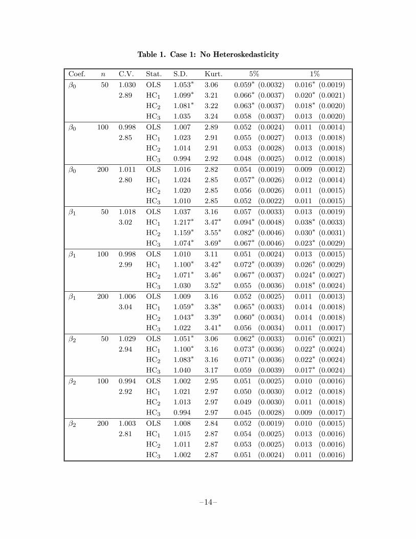
Table 1. Case 1: No Heteroskedasticity

Coef. n C.V. Stat. S.D. Kurt. 5% 1%

β0 50 1.030 OLS 1.053∗ 3.06 0.059∗ (0.0032) 0.016∗ (0.0019)

2.89 HC1 1.099∗ 3.21 0.066∗ (0.0037) 0.020∗ (0.0021)

HC2 1.081∗ 3.22 0.063∗ (0.0037) 0.018∗ (0.0020)

HC3 1.035 3.24 0.058 (0.0037) 0.013 (0.0020)

β0 100 0.998 OLS 1.007 2.89 0.052 (0.0024) 0.011 (0.0014)

2.85 HC1 1.023 2.91 0.055 (0.0027) 0.013 (0.0018)

HC2 1.014 2.91 0.053 (0.0028) 0.013 (0.0018)

HC3 0.994 2.92 0.048 (0.0025) 0.012 (0.0018)

β0 200 1.011 OLS 1.016 2.82 0.054 (0.0019) 0.009 (0.0012)

2.80 HC1 1.024 2.85 0.057∗ (0.0026) 0.012 (0.0014)

HC2 1.020 2.85 0.056 (0.0026) 0.011 (0.0015)

HC3 1.010 2.85 0.052 (0.0022) 0.011 (0.0015)

β1 50 1.018 OLS 1.037 3.16 0.057 (0.0033) 0.013 (0.0019)

3.02 HC1 1.217∗ 3.47∗ 0.094∗ (0.0048) 0.038∗ (0.0033)

HC2 1.159∗ 3.55∗ 0.082∗ (0.0046) 0.030∗ (0.0031)

HC3 1.074∗ 3.69∗ 0.067∗ (0.0046) 0.023∗ (0.0029)

β1 100 0.998 OLS 1.010 3.11 0.051 (0.0024) 0.013 (0.0015)

2.99 HC1 1.100∗ 3.42∗ 0.072∗ (0.0039) 0.026∗ (0.0029)

HC2 1.071∗ 3.46∗ 0.067∗ (0.0037) 0.024∗ (0.0027)

HC3 1.030 3.52∗ 0.055 (0.0036) 0.018∗ (0.0024)

β1 200 1.006 OLS 1.009 3.16 0.052 (0.0025) 0.011 (0.0013)

3.04 HC1 1.059∗ 3.38∗ 0.065∗ (0.0033) 0.014 (0.0018)

HC2 1.043∗ 3.39∗ 0.060∗ (0.0034) 0.014 (0.0018)

HC3 1.022 3.41∗ 0.056 (0.0034) 0.011 (0.0017)

β2 50 1.029 OLS 1.051∗ 3.06 0.062∗ (0.0033) 0.016∗ (0.0021)

2.94 HC1 1.100∗ 3.16 0.073∗ (0.0036) 0.022∗ (0.0024)

HC2 1.083∗ 3.16 0.071∗ (0.0036) 0.022∗ (0.0024)

HC3 1.040 3.17 0.059 (0.0039) 0.017∗ (0.0024)

β2 100 0.994 OLS 1.002 2.95 0.051 (0.0025) 0.010 (0.0016)

2.92 HC1 1.021 2.97 0.050 (0.0030) 0.012 (0.0018)

HC2 1.013 2.97 0.049 (0.0030) 0.011 (0.0018)

HC3 0.994 2.97 0.045 (0.0028) 0.009 (0.0017)

β2 200 1.003 OLS 1.008 2.84 0.052 (0.0019) 0.010 (0.0015)

2.81 HC1 1.015 2.87 0.054 (0.0025) 0.013 (0.0016)

HC2 1.011 2.87 0.053 (0.0025) 0.013 (0.0016)

HC3 1.002 2.87 0.051 (0.0024) 0.011 (0.0016)

–14–

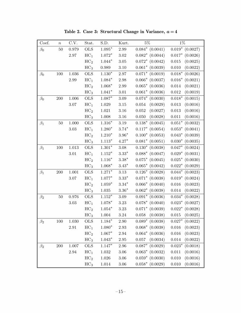
Table 2. Case 3: Structural Change in Variance, a=4

Coef. n C.V. Stat. S.D. Kurt. 5% 1%

β0 50 0.979 OLS 1.095∗ 2.99 0.084∗ (0.0041) 0.019∗ (0.0027)

2.97 HC1 1.072∗ 3.02 0.082∗ (0.0044) 0.017∗ (0.0026)

HC2 1.044∗ 3.05 0.072∗ (0.0042) 0.015 (0.0025)

HC3 0.989 3.10 0.061∗ (0.0039) 0.010 (0.0022)

β0 100 1.036 OLS 1.130∗ 2.97 0.071∗ (0.0019) 0.018∗ (0.0026)

2.99 HC1 1.084∗ 2.98 0.066∗ (0.0037) 0.016∗ (0.0021)

HC2 1.068∗ 2.99 0.065∗ (0.0036) 0.014 (0.0021)

HC3 1.041∗ 3.01 0.061∗ (0.0036) 0.012 (0.0019)

β0 200 1.006 OLS 1.087∗ 3.09 0.074∗ (0.0030) 0.018∗ (0.0015)

3.07 HC1 1.029 3.15 0.054 (0.0029) 0.013 (0.0016)

HC2 1.021 3.16 0.052 (0.0027) 0.013 (0.0016)

HC3 1.008 3.16 0.050 (0.0028) 0.011 (0.0016)

β1 50 1.000 OLS 1.316∗ 3.19 0.138∗ (0.0045) 0.051∗ (0.0032)

3.03 HC1 1.280∗ 3.74∗ 0.117∗ (0.0054) 0.053∗ (0.0041)

HC2 1.210∗ 3.96∗ 0.100∗ (0.0053) 0.043∗ (0.0039)

HC3 1.113∗ 4.27∗ 0.081∗ (0.0051) 0.030∗ (0.0035)

β1 100 1.013 OLS 1.301∗ 3.08 0.130∗ (0.0038) 0.047∗ (0.0024)

3.01 HC1 1.152∗ 3.33∗ 0.088∗ (0.0047) 0.029∗ (0.0031)

HC2 1.116∗ 3.38∗ 0.075∗ (0.0045) 0.025∗ (0.0030)

HC3 1.068∗ 3.43∗ 0.065∗ (0.0042) 0.022∗ (0.0029)

β1 200 1.001 OLS 1.271∗ 3.13 0.126∗ (0.0028) 0.044∗ (0.0023)

3.07 HC1 1.077∗ 3.33∗ 0.071∗ (0.0038) 0.019∗ (0.0024)

HC2 1.059∗ 3.34∗ 0.066∗ (0.0040) 0.016 (0.0023)

HC3 1.035 3.36∗ 0.062∗ (0.0038) 0.014 (0.0022)

β2 50 0.976 OLS 1.152∗ 3.09 0.091∗ (0.0036) 0.034∗ (0.0028)

3.03 HC1 1.078∗ 3.23 0.078∗ (0.0040) 0.023∗ (0.0027)

HC2 1.054∗ 3.23 0.071∗ (0.0039) 0.022∗ (0.0028)

HC3 1.004 3.24 0.058 (0.0038) 0.015 (0.0025)

β2 100 1.030 OLS 1.184∗ 2.90 0.089∗ (0.0038) 0.027∗ (0.0022)

2.91 HC1 1.080∗ 2.93 0.068∗ (0.0038) 0.016 (0.0023)

HC2 1.067∗ 2.94 0.064∗ (0.0036) 0.016 (0.0023)

HC3 1.043∗ 2.95 0.057 (0.0034) 0.014 (0.0022)

β2 200 1.007 OLS 1.147∗ 2.96 0.087∗ (0.0029) 0.023∗ (0.0018)

2.94 HC1 1.032 3.06 0.063∗ (0.0032) 0.011 (0.0016)

HC2 1.026 3.06 0.059∗ (0.0030) 0.010 (0.0016)

HC3 1.014 3.06 0.058∗ (0.0029) 0.010 (0.0016)

–15–

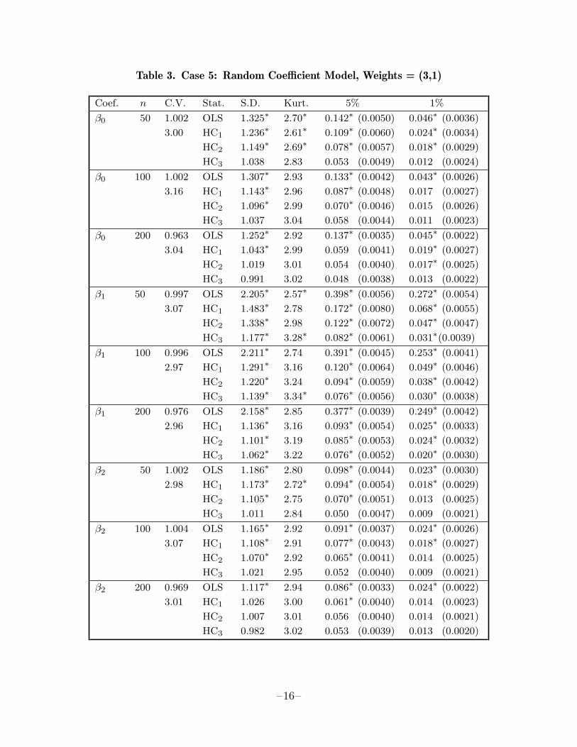
Table 3. Case 5: Random Coefficient Model, Weights = (3,1)

Coef. n C.V. Stat. S.D. Kurt. 5% 1%

β0 50 1.002 OLS 1.325∗ 2.70∗ 0.142∗ (0.0050) 0.046∗ (0.0036)

3.00 HC1 1.236∗ 2.61∗ 0.109∗ (0.0060) 0.024∗ (0.0034)

HC2 1.149∗ 2.69∗ 0.078∗ (0.0057) 0.018∗ (0.0029)

HC3 1.038 2.83 0.053 (0.0049) 0.012 (0.0024)

β0 100 1.002 OLS 1.307∗ 2.93 0.133∗ (0.0042) 0.043∗ (0.0026)

3.16 HC1 1.143∗ 2.96 0.087∗ (0.0048) 0.017 (0.0027)

HC2 1.096∗ 2.99 0.070∗ (0.0046) 0.015 (0.0026)

HC3 1.037 3.04 0.058 (0.0044) 0.011 (0.0023)

β0 200 0.963 OLS 1.252∗ 2.92 0.137∗ (0.0035) 0.045∗ (0.0022)

3.04 HC1 1.043∗ 2.99 0.059 (0.0041) 0.019∗ (0.0027)

HC2 1.019 3.01 0.054 (0.0040) 0.017∗ (0.0025)

HC3 0.991 3.02 0.048 (0.0038) 0.013 (0.0022)

β1 50 0.997 OLS 2.205∗ 2.57∗ 0.398∗ (0.0056) 0.272∗ (0.0054)

3.07 HC1 1.483∗ 2.78 0.172∗ (0.0080) 0.068∗ (0.0055)

HC2 1.338∗ 2.98 0.122∗ (0.0072) 0.047∗ (0.0047)

HC3 1.177∗ 3.28∗ 0.082∗ (0.0061) 0.031∗(0.0039)

β1 100 0.996 OLS 2.211∗ 2.74 0.391∗ (0.0045) 0.253∗ (0.0041)

2.97 HC1 1.291∗ 3.16 0.120∗ (0.0064) 0.049∗ (0.0046)

HC2 1.220∗ 3.24 0.094∗ (0.0059) 0.038∗ (0.0042)

HC3 1.139∗ 3.34∗ 0.076∗ (0.0056) 0.030∗ (0.0038)

β1 200 0.976 OLS 2.158∗ 2.85 0.377∗ (0.0039) 0.249∗ (0.0042)

2.96 HC1 1.136∗ 3.16 0.093∗ (0.0054) 0.025∗ (0.0033)

HC2 1.101∗ 3.19 0.085∗ (0.0053) 0.024∗ (0.0032)

HC3 1.062∗ 3.22 0.076∗ (0.0052) 0.020∗ (0.0030)

β2 50 1.002 OLS 1.186∗ 2.80 0.098∗ (0.0044) 0.023∗ (0.0030)

2.98 HC1 1.173∗ 2.72∗ 0.094∗ (0.0054) 0.018∗ (0.0029)

HC2 1.105∗ 2.75 0.070∗ (0.0051) 0.013 (0.0025)

HC3 1.011 2.84 0.050 (0.0047) 0.009 (0.0021)

β2 100 1.004 OLS 1.165∗ 2.92 0.091∗ (0.0037) 0.024∗ (0.0026)

3.07 HC1 1.108∗ 2.91 0.077∗ (0.0043) 0.018∗ (0.0027)

HC2 1.070∗ 2.92 0.065∗ (0.0041) 0.014 (0.0025)

HC3 1.021 2.95 0.052 (0.0040) 0.009 (0.0021)

β2 200 0.969 OLS 1.117∗ 2.94 0.086∗ (0.0033) 0.024∗ (0.0022)

3.01 HC1 1.026 3.00 0.061∗ (0.0040) 0.014 (0.0023)

HC2 1.007 3.01 0.056 (0.0040) 0.014 (0.0021)

HC3 0.982 3.02 0.053 (0.0039) 0.013 (0.0020)

–16–

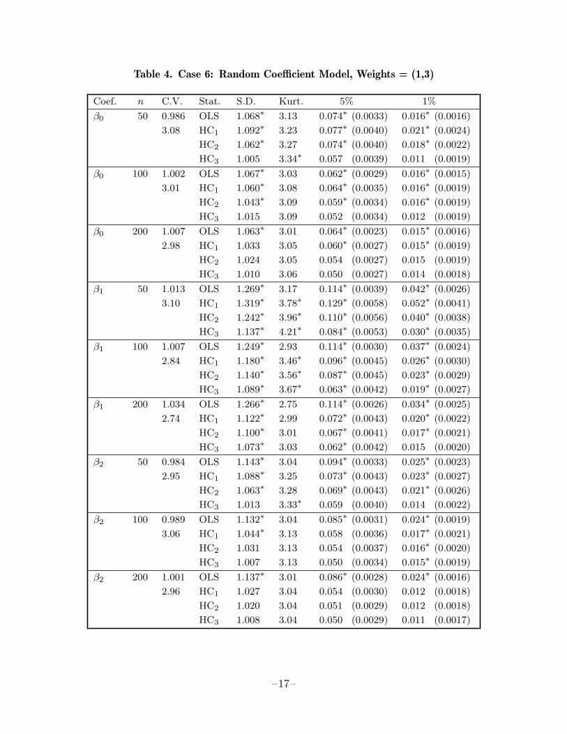
Table 4. Case 6: Random Coefficient Model, Weights = (1,3)

Coef. n C.V. Stat. S.D. Kurt. 5% 1%

β0 50 0.986 OLS 1.068∗ 3.13 0.074∗ (0.0033) 0.016∗ (0.0016)

3.08 HC1 1.092∗ 3.23 0.077∗ (0.0040) 0.021∗ (0.0024)

HC2 1.062∗ 3.27 0.074∗ (0.0040) 0.018∗ (0.0022)

HC3 1.005 3.34∗ 0.057 (0.0039) 0.011 (0.0019)

β0 100 1.002 OLS 1.067∗ 3.03 0.062∗ (0.0029) 0.016∗ (0.0015)

3.01 HC1 1.060∗ 3.08 0.064∗ (0.0035) 0.016∗ (0.0019)

HC2 1.043∗ 3.09 0.059∗ (0.0034) 0.016∗ (0.0019)

HC3 1.015 3.09 0.052 (0.0034) 0.012 (0.0019)

β0 200 1.007 OLS 1.063∗ 3.01 0.064∗ (0.0023) 0.015∗ (0.0016)

2.98 HC1 1.033 3.05 0.060∗ (0.0027) 0.015∗ (0.0019)

HC2 1.024 3.05 0.054 (0.0027) 0.015 (0.0019)

HC3 1.010 3.06 0.050 (0.0027) 0.014 (0.0018)

β1 50 1.013 OLS 1.269∗ 3.17 0.114∗ (0.0039) 0.042∗ (0.0026)

3.10 HC1 1.319∗ 3.78∗ 0.129∗ (0.0058) 0.052∗ (0.0041)

HC2 1.242∗ 3.96∗ 0.110∗ (0.0056) 0.040∗ (0.0038)

HC3 1.137∗ 4.21∗ 0.084∗ (0.0053) 0.030∗ (0.0035)

β1 100 1.007 OLS 1.249∗ 2.93 0.114∗ (0.0030) 0.037∗ (0.0024)

2.84 HC1 1.180∗ 3.46∗ 0.096∗ (0.0045) 0.026∗ (0.0030)

HC2 1.140∗ 3.56∗ 0.087∗ (0.0045) 0.023∗ (0.0029)

HC3 1.089∗ 3.67∗ 0.063∗ (0.0042) 0.019∗ (0.0027)

β1 200 1.034 OLS 1.266∗ 2.75 0.114∗ (0.0026) 0.034∗ (0.0025)

2.74 HC1 1.122∗ 2.99 0.072∗ (0.0043) 0.020∗ (0.0022)

HC2 1.100∗ 3.01 0.067∗ (0.0041) 0.017∗ (0.0021)

HC3 1.073∗ 3.03 0.062∗ (0.0042) 0.015 (0.0020)

β2 50 0.984 OLS 1.143∗ 3.04 0.094∗ (0.0033) 0.025∗ (0.0023)

2.95 HC1 1.088∗ 3.25 0.073∗ (0.0043) 0.023∗ (0.0027)

HC2 1.063∗ 3.28 0.069∗ (0.0043) 0.021∗ (0.0026)

HC3 1.013 3.33∗ 0.059 (0.0040) 0.014 (0.0022)

β2 100 0.989 OLS 1.132∗ 3.04 0.085∗ (0.0031) 0.024∗ (0.0019)

3.06 HC1 1.044∗ 3.13 0.058 (0.0036) 0.017∗ (0.0021)

HC2 1.031 3.13 0.054 (0.0037) 0.016∗ (0.0020)

HC3 1.007 3.13 0.050 (0.0034) 0.015∗ (0.0019)

β2 200 1.001 OLS 1.137∗ 3.01 0.086∗ (0.0028) 0.024∗ (0.0016)

2.96 HC1 1.027 3.04 0.054 (0.0030) 0.012 (0.0018)

HC2 1.020 3.04 0.051 (0.0029) 0.012 (0.0018)

HC3 1.008 3.04 0.050 (0.0029) 0.011 (0.0017)

–17–

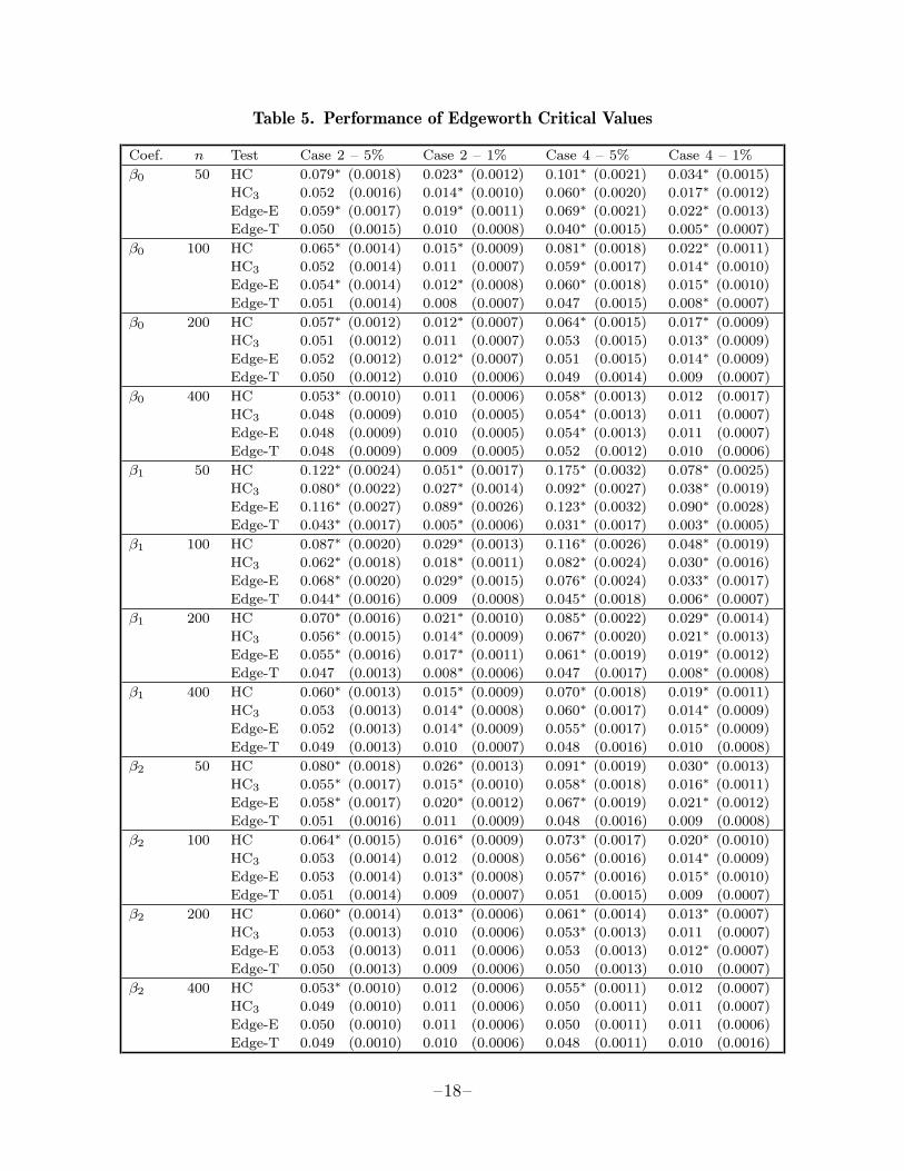
Table 5. Performance of Edgeworth Critical Values

Coef. n Test Case 2 – 5% Case 2 – 1% Case 4 – 5% Case 4 – 1%

β0 50 HC 0.079∗ (0.0018) 0.023∗ (0.0012) 0.101∗ (0.0021) 0.034∗ (0.0015)

HC3 0.052 (0.0016) 0.014∗ (0.0010) 0.060∗ (0.0020) 0.017∗ (0.0012)

Edge-E 0.059∗ (0.0017) 0.019∗ (0.0011) 0.069∗ (0.0021) 0.022∗ (0.0013)

Edge-T 0.050 (0.0015) 0.010 (0.0008) 0.040∗ (0.0015) 0.005∗ (0.0007)

β0 100 HC 0.065∗ (0.0014) 0.015∗ (0.0009) 0.081∗ (0.0018) 0.022∗ (0.0011)

HC3 0.052 (0.0014) 0.011 (0.0007) 0.059∗ (0.0017) 0.014∗ (0.0010)

Edge-E 0.054∗ (0.0014) 0.012∗ (0.0008) 0.060∗ (0.0018) 0.015∗ (0.0010)

Edge-T 0.051 (0.0014) 0.008 (0.0007) 0.047 (0.0015) 0.008∗ (0.0007)

β0 200 HC 0.057∗ (0.0012) 0.012∗ (0.0007) 0.064∗ (0.0015) 0.017∗ (0.0009)

HC3 0.051 (0.0012) 0.011 (0.0007) 0.053 (0.0015) 0.013∗ (0.0009)

Edge-E 0.052 (0.0012) 0.012∗ (0.0007) 0.051 (0.0015) 0.014∗ (0.0009)

Edge-T 0.050 (0.0012) 0.010 (0.0006) 0.049 (0.0014) 0.009 (0.0007)

β0 400 HC 0.053∗ (0.0010) 0.011 (0.0006) 0.058∗ (0.0013) 0.012 (0.0017)

HC3 0.048 (0.0009) 0.010 (0.0005) 0.054∗ (0.0013) 0.011 (0.0007)

Edge-E 0.048 (0.0009) 0.010 (0.0005) 0.054∗ (0.0013) 0.011 (0.0007)

Edge-T 0.048 (0.0009) 0.009 (0.0005) 0.052 (0.0012) 0.010 (0.0006)

β1 50 HC 0.122∗ (0.0024) 0.051∗ (0.0017) 0.175∗ (0.0032) 0.078∗ (0.0025)

HC3 0.080∗ (0.0022) 0.027∗ (0.0014) 0.092∗ (0.0027) 0.038∗ (0.0019)

Edge-E 0.116∗ (0.0027) 0.089∗ (0.0026) 0.123∗ (0.0032) 0.090∗ (0.0028)

Edge-T 0.043∗ (0.0017) 0.005∗ (0.0006) 0.031∗ (0.0017) 0.003∗ (0.0005)

β1 100 HC 0.087∗ (0.0020) 0.029∗ (0.0013) 0.116∗ (0.0026) 0.048∗ (0.0019)

HC3 0.062∗ (0.0018) 0.018∗ (0.0011) 0.082∗ (0.0024) 0.030∗ (0.0016)

Edge-E 0.068∗ (0.0020) 0.029∗ (0.0015) 0.076∗ (0.0024) 0.033∗ (0.0017)

Edge-T 0.044∗ (0.0016) 0.009 (0.0008) 0.045∗ (0.0018) 0.006∗ (0.0007)

β1 200 HC 0.070∗ (0.0016) 0.021∗ (0.0010) 0.085∗ (0.0022) 0.029∗ (0.0014)

HC3 0.056∗ (0.0015) 0.014∗ (0.0009) 0.067∗ (0.0020) 0.021∗ (0.0013)

Edge-E 0.055∗ (0.0016) 0.017∗ (0.0011) 0.061∗ (0.0019) 0.019∗ (0.0012)

Edge-T 0.047 (0.0013) 0.008∗ (0.0006) 0.047 (0.0017) 0.008∗ (0.0008)

β1 400 HC 0.060∗ (0.0013) 0.015∗ (0.0009) 0.070∗ (0.0018) 0.019∗ (0.0011)

HC3 0.053 (0.0013) 0.014∗ (0.0008) 0.060∗ (0.0017) 0.014∗ (0.0009)

Edge-E 0.052 (0.0013) 0.014∗ (0.0009) 0.055∗ (0.0017) 0.015∗ (0.0009)

Edge-T 0.049 (0.0013) 0.010 (0.0007) 0.048 (0.0016) 0.010 (0.0008)

β2 50 HC 0.080∗ (0.0018) 0.026∗ (0.0013) 0.091∗ (0.0019) 0.030∗ (0.0013)

HC3 0.055∗ (0.0017) 0.015∗ (0.0010) 0.058∗ (0.0018) 0.016∗ (0.0011)

Edge-E 0.058∗ (0.0017) 0.020∗ (0.0012) 0.067∗ (0.0019) 0.021∗ (0.0012)

Edge-T 0.051 (0.0016) 0.011 (0.0009) 0.048 (0.0016) 0.009 (0.0008)

β2 100 HC 0.064∗ (0.0015) 0.016∗ (0.0009) 0.073∗ (0.0017) 0.020∗ (0.0010)

HC3 0.053 (0.0014) 0.012 (0.0008) 0.056∗ (0.0016) 0.014∗ (0.0009)

Edge-E 0.053 (0.0014) 0.013∗ (0.0008) 0.057∗ (0.0016) 0.015∗ (0.0010)

Edge-T 0.051 (0.0014) 0.009 (0.0007) 0.051 (0.0015) 0.009 (0.0007)

β2 200 HC 0.060∗ (0.0014) 0.013∗ (0.0006) 0.061∗ (0.0014) 0.013∗ (0.0007)

HC3 0.053 (0.0013) 0.010 (0.0006) 0.053∗ (0.0013) 0.011 (0.0007)

Edge-E 0.053 (0.0013) 0.011 (0.0006) 0.053 (0.0013) 0.012∗ (0.0007)

Edge-T 0.050 (0.0013) 0.009 (0.0006) 0.050 (0.0013) 0.010 (0.0007)

β2 400 HC 0.053∗ (0.0010) 0.012 (0.0006) 0.055∗ (0.0011) 0.012 (0.0007)

HC3 0.049 (0.0010) 0.011 (0.0006) 0.050 (0.0011) 0.011 (0.0007)

Edge-E 0.050 (0.0010) 0.011 (0.0006) 0.050 (0.0011) 0.011 (0.0006)

Edge-T 0.049 (0.0010) 0.010 (0.0006) 0.048 (0.0011) 0.010 (0.0016)

–18–

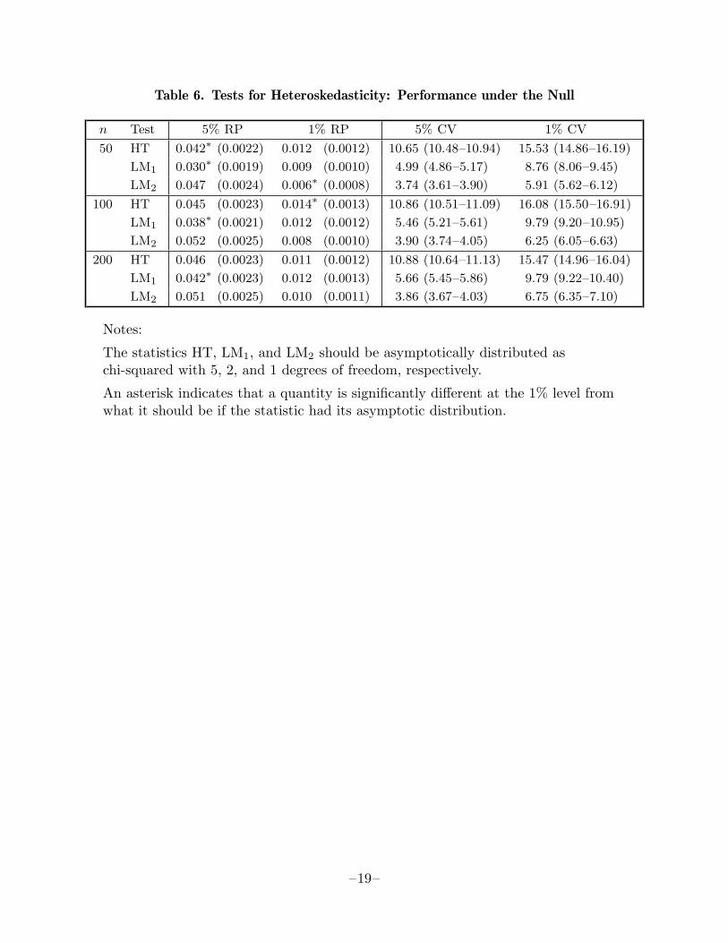
Table 6. Tests for Heteroskedasticity: Performance under the Null

n Test 5% RP 1% RP 5% CV 1% CV

50 HT 0.042∗ (0.0022) 0.012 (0.0012) 10.65 (10.48–10.94) 15.53 (14.86–16.19)

LM1 0.030∗ (0.0019) 0.009 (0.0010) 4.99 (4.86–5.17) 8.76 (8.06–9.45)

LM2 0.047 (0.0024) 0.006∗ (0.0008) 3.74 (3.61–3.90) 5.91 (5.62–6.12)

100 HT 0.045 (0.0023) 0.014∗ (0.0013) 10.86 (10.51–11.09) 16.08 (15.50–16.91)

LM1 0.038∗ (0.0021) 0.012 (0.0012) 5.46 (5.21–5.61) 9.79 (9.20–10.95)

LM2 0.052 (0.0025) 0.008 (0.0010) 3.90 (3.74–4.05) 6.25 (6.05–6.63)

200 HT 0.046 (0.0023) 0.011 (0.0012) 10.88 (10.64–11.13) 15.47 (14.96–16.04)

LM1 0.042∗ (0.0023) 0.012 (0.0013) 5.66 (5.45–5.86) 9.79 (9.22–10.40)

LM2 0.051 (0.0025) 0.010 (0.0011) 3.86 (3.67–4.03) 6.75 (6.35–7.10)

Notes:

The statistics HT, LM1, and LM2 should be asymptotically distributed aschi-squared with 5, 2, and 1 degrees of freedom, respectively.

An asterisk indicates that a quantity is significantly different at the 1% level fromwhat it should be if the statistic had its asymptotic distribution.

–19–

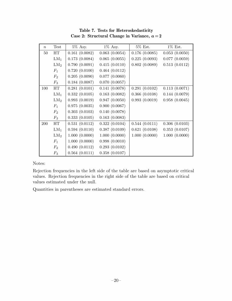
Table 7. Tests for HeteroskedasticityCase 2: Structural Change in Variance, a=2

n Test 5% Asy. 1% Asy. 5% Est. 1% Est.

50 HT 0.161 (0.0082) 0.063 (0.0054) 0.176 (0.0085) 0.053 (0.0050)

LM1 0.173 (0.0084) 0.065 (0.0055) 0.225 (0.0093) 0.077 (0.0059)

LM2 0.790 (0.0091) 0.415 (0.0110) 0.802 (0.0089) 0.513 (0.0112)

F1 0.720 (0.0100) 0.464 (0.0112)

F2 0.205 (0.0090) 0.077 (0.0060)

F3 0.184 (0.0087) 0.070 (0.0057)

100 HT 0.281 (0.0101) 0.141 (0.0078) 0.291 (0.0102) 0.113 (0.0071)

LM1 0.332 (0.0105) 0.163 (0.0082) 0.366 (0.0108) 0.144 (0.0079)

LM2 0.993 (0.0019) 0.947 (0.0050) 0.993 (0.0019) 0.958 (0.0045)

F1 0.975 (0.0035) 0.900 (0.0067)

F2 0.303 (0.0103) 0.140 (0.0078)

F3 0.333 (0.0105) 0.163 (0.0083)

200 HT 0.531 (0.0112) 0.322 (0.0104) 0.544 (0.0111) 0.306 (0.0103)

LM1 0.594 (0.0110) 0.387 (0.0109) 0.621 (0.0108) 0.353 (0.0107)

LM2 1.000 (0.0000) 1.000 (0.0000) 1.000 (0.0000) 1.000 (0.0000)

F1 1.000 (0.0000) 0.998 (0.0010)

F2 0.490 (0.0112) 0.293 (0.0102)

F3 0.564 (0.0111) 0.358 (0.0107)

Notes:

Rejection frequencies in the left side of the table are based on asymptotic criticalvalues. Rejection frequencies in the right side of the table are based on criticalvalues estimated under the null.

Quantities in parentheses are estimated standard errors.

–20–

Table 8. Tests for HeteroskedasticityCase 4: Random Coefficient Model, Weights = (1,1)

n Test 5% Asy. 1% Asy. 5% Est. 1% Est.

50 HT 0.281 (0.0100) 0.152 (0.0080) 0.295 (0.0102) 0.145 (0.0079)

LM1 0.267 (0.0099) 0.170 (0.0084) 0.314 (0.0104) 0.185 (0.0087)

LM2 0.056 (0.0051) 0.009 (0.0021) 0.060 (0.0053) 0.015 (0.0027)

F1 0.100 (0.0067) 0.024 (0.0034)

F2 0.090 (0.0064) 0.027 (0.0036)

F3 0.081 (0.0061) 0.017 (0.0028)

100 HT 0.560 (0.0111) 0.419 (0.0110) 0.570 (0.0111) 0.385 (0.0109)

LM1 0.567 (0.0111) 0.446 (0.0111) 0.591 (0.0110) 0.424 (0.0111)

LM2 0.097 (0.0066) 0.015 (0.0027) 0.096 (0.0066) 0.022 (0.0032)

F1 0.202 (0.0090) 0.083 (0.0062)

F2 0.202 (0.0090) 0.076 (0.0059)

F3 0.104 (0.0068) 0.029 (0.0037)

200 HT 0.870 (0.0075) 0.760 (0.0096) 0.877 (0.0073) 0.748 (0.0097)

LM1 0.853 (0.0079) 0.767 (0.0095) 0.862 (0.0077) 0.749 (0.0097)

LM2 0.180 (0.0086) 0.039 (0.0043) 0.178 (0.0086) 0.035 (0.0041)

F1 0.369 (0.0108) 0.183 (0.0086)

F2 0.384 (0.0109) 0.202 (0.0090)

F3 0.141 (0.0078) 0.048 (0.0048)

Notes:

Rejection frequencies in the left side of the table are based on asymptotic criticalvalues. Rejection frequencies in the right side of the table are based on criticalvalues estimated under the null.

Quantities in parentheses are estimated standard errors.

–21–

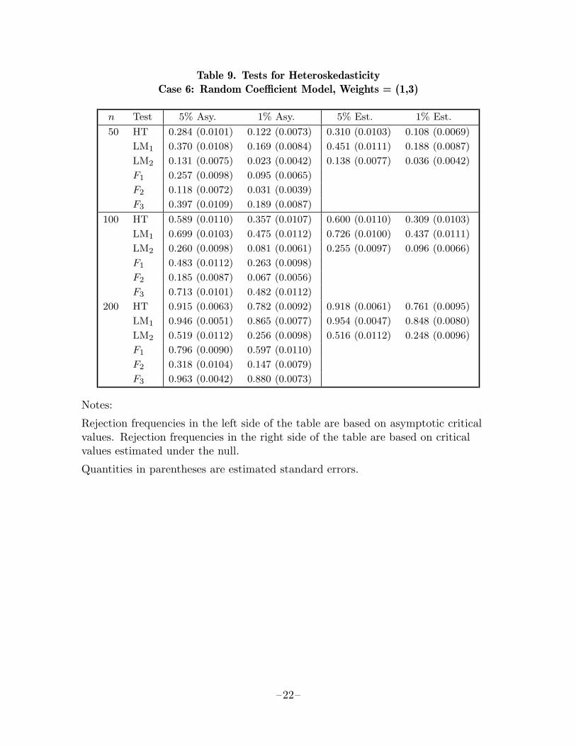
Table 9. Tests for HeteroskedasticityCase 6: Random Coefficient Model, Weights = (1,3)

n Test 5% Asy. 1% Asy. 5% Est. 1% Est.

50 HT 0.284 (0.0101) 0.122 (0.0073) 0.310 (0.0103) 0.108 (0.0069)

LM1 0.370 (0.0108) 0.169 (0.0084) 0.451 (0.0111) 0.188 (0.0087)

LM2 0.131 (0.0075) 0.023 (0.0042) 0.138 (0.0077) 0.036 (0.0042)

F1 0.257 (0.0098) 0.095 (0.0065)

F2 0.118 (0.0072) 0.031 (0.0039)

F3 0.397 (0.0109) 0.189 (0.0087)

100 HT 0.589 (0.0110) 0.357 (0.0107) 0.600 (0.0110) 0.309 (0.0103)

LM1 0.699 (0.0103) 0.475 (0.0112) 0.726 (0.0100) 0.437 (0.0111)

LM2 0.260 (0.0098) 0.081 (0.0061) 0.255 (0.0097) 0.096 (0.0066)

F1 0.483 (0.0112) 0.263 (0.0098)

F2 0.185 (0.0087) 0.067 (0.0056)

F3 0.713 (0.0101) 0.482 (0.0112)

200 HT 0.915 (0.0063) 0.782 (0.0092) 0.918 (0.0061) 0.761 (0.0095)

LM1 0.946 (0.0051) 0.865 (0.0077) 0.954 (0.0047) 0.848 (0.0080)

LM2 0.519 (0.0112) 0.256 (0.0098) 0.516 (0.0112) 0.248 (0.0096)

F1 0.796 (0.0090) 0.597 (0.0110)

F2 0.318 (0.0104) 0.147 (0.0079)

F3 0.963 (0.0042) 0.880 (0.0073)

Notes:

Rejection frequencies in the left side of the table are based on asymptotic criticalvalues. Rejection frequencies in the right side of the table are based on criticalvalues estimated under the null.

Quantities in parentheses are estimated standard errors.

–22–