Assessing the Benefits of Integrated Vehicle Life Cycle Planning

Wendy Lu XuBarry L. Nelson

Northwestern University

Wallace J. HoppUniversity of Michigan

Jonathan H. OwenGeneral Motors R&D

February 15, 2009

Abstract

Many decisions are involved in managing the vehicle life cycle. These include product portfolioplanning (which models to launch at which times), plant assignment (which plants to use toproduce each vehicle) and production allocation (how much of each vehicle to produce in eachplant). Since these decisions are complex and made at different points in time they are typicallydecoupled in practice. But they clearly impact one another, since portfolio decisions constrainassignment decisions, which in turn constrain the allocation decisions. We present a MarkovDecision Process model, which maximizes expected long-run average profit, to assess the value ofintegrating portfolio planning and plant assignment. Our analytical and numerical results suggestthat decoupling these decisions can lead to substantial loss of profit, particularly when plantcapacity utilization is moderate and flexible tooling makes it significantly cheaper to introducenew models into plants.

Keywords: Product Portfolio Planning, Product-to-Plant Assignment, Markov Decision Pro-cesses.

1 Introduction

Introduction of new and updated vehicles is one of the most vital activities of an automotive

company. Without a steady stream of offerings that are perceived by the buying public as “new”

and “fresh” within a segment, a firm cannot remain competitive. No amount of manufacturing

efficiency or quality control can offset the disadvantage of having “stale” products. As a result, all

automotive companies devote a tremendous amount of managerial attention at all levels, including

in the executive suite, to the problem of planning the evolution of their vehicle portfolio over time.

A central issue in this planning process is when to refresh or replace models.

1

On the surface, this looks like a marketing problem. The firm must be sensitive to customer

tastes (e.g., “freshness” may be more important to buyers of a stylish sports car than to buyers of a

utilitarian pickup). It must also take into account the pace of innovation by the competition. With

these, the firm can predict the decline in demand for a model as it ages and balance this with the

cost of design and tooling needed to launch a refreshed model to determine an appropriate refresh

cycle.

But this problem goes well beyond marketing. Decisions about when and how often to re-

fresh/replace models impact the workload on engineering resources, as well as the options for where

the vehicles can be produced. Decisions about the assignment of vehicles to plants in turn affect

subsequent decisions about how many vehicles of each type to produce in each plant.

To cope with the scale and complexity of this multidimensional planning problem, firms generally

decouple the portfolio problem from the downstream decisions it impacts. That is, the portfolio

problem is solved primarily as a marketing problem, with some checks on the resource implications

of the decisions. For instance, to ensure that engineering resources are not overtaxed, the firm may

restrict the number of major and minor refreshes in a given year to not exceed a specified number

as a rough approximation.

But accounting for plant assignment considerations is more subtle because the life cycle cost of

refreshing can depend on where the vehicle is produced, as well as where other vehicles are produced

(i.e., because plant capacities may be shared by multiple vehicles). It would be simple to assume

that a refreshed model will be produced in the same plant(s) as the old model it replaces. But

this will not always be the best solution due to plant closings to consolidate capacity, new plant

construction to add capacity or technology, improvements in flexibility that make it feasible to

produce more models in a single plant and other business trends. Consequently, portfolio planners

do not always know where a model will be produced at the time a refresh is planned. Therefore,

they typically assume average tooling and production costs to evaluate the economics of replacement

decisions. The actual costs will not be revealed until after the assignments are made and production

is scheduled.

Because portfolio decisions influence plant assignment decisions, which in turn influence produc-

2

tion allocation decisions, decoupling may lead to suboptimal decisions. This presents the following

questions:

1. How large can the shortfall in expected profit be from decoupling portfolio planning from

plant assignment and production allocation?

2. Under what conditions is decoupling the decisions likely to lead to large profit shortfall, and

when is such decoupling likely to result in good performance?

3. How can planners incorporate implications for the downstream plant assignment and produc-

tion allocation decisions into the portfolio planning process?

In this paper, we address the first two questions in some detail and provide the basis for a

method to address the third. To do this, we develop a Markov Decision Process (MDP) model that

integrates portfolio planning, vehicle assignment and production allocation.

There is a considerable body of literature on new product development/R&D project portfolio

planning which addresses the problem of allocating limited resources to products/projects in a way

that maximizes the return, provides balance, and aligns with the strategy of the enterprise. Heiden-

berger and Stummer (1999) gave a comprehensive review of approaches to quantitative modeling for

project selection and resource allocation, which include benefit measurement methods, mathemati-

cal programming, and other techniques. Other methods include graphical and charting techniques.

Cooper et al. (1999) reported the portfolio management practices and performances of 205 U.S.

companies. Dickinson et al. (2001), Loch and Kavadias (2002) and Stummer and Heidenberger

(2003) addressed the portfolio problem over multiple periods. But none of these computed the

return for new products/projects by taking into account downstream manufacturing decisions.

The way we model the portfolio decision process has some similarity to the work on machine

maintenance problems. Surveys of the maintenance/replacement literature include Barlow et al.

(1965), MacCall (1965), Pierskalla and Voelker (1976), Sherif and Smith (1981), Valdez-Flores and

Feldman (1989) and Wang (2002). Decreasing demand over time in our model is analogous to

deteriorating system performance in maintenance models. Vehicle model refresh, which is aimed

3

at increasing demand, is similar to maintenance, which is intended to increase performance. Ac-

cording to the classification of maintenance models in Pierskalla and Voelker (1976) and Wang

(2002), our portfolio decision problem is similar to a discrete-time maintenance model with a single

maintenance action, complete information and no inspection, which can be formulated as a Markov

Decision Process with a failure limit policy. Among the machine maintenance studies, Sloan and

Shanthikumar (2000) is most similar to our problem in that it models maintenance and production

schedules simultaneously. The difference between our model and their work is that they decide

either to perform maintenance or to produce one of several alternative products, while in our model

we decide whether to refresh a vehicle and where to assign it at the same time, with production

planning as a second-stage decision. Also our measure of performance includes revenue, which is

determined by production quantity and is not a decision variable in their model.

Plant assignment and production planning is a complicated problem that must take into account

timing of product introductions, limited tooling of each product, limited capacity of plants, and

other issues. Inman and Gonsalvez (2001) described a tool for optimizing the allocation of vehicle

products to plants considering the capacity constraints of individual lines, body shops and plants,

with the objective of minimizing lost sales, equalizing utilization among plants, and maximizing the

amount of inter-plant chaining. Alden, Costy and Inman (2002) presented a decision support tool

to assess the cost of plant modifications needed to build a new vehicle product. In our model, plant

assignment is a decision in the MDP associated with tooling costs, while production planning is

formulated as a linear optimization problem.

The remainder of the paper is organized as follows: Section 2 formulates two MDP models for a

two-plant, two-product system, one for the case where the portfolio planning decision is integrated

with the plant assignment and production allocation decisions, and one where they are decoupled.

This section also gives basic structural results for the optimal policies. Section 3 presents a numerical

analysis that investigates the size and causes of large shortfall between the results of the integrated

and decoupled models. Section 4 summarizes our conclusions, which are:

1. The shortfall in expected profit from failing to integrate plant assignment and product allo-

4

cation considerations into the portfolio planning process can be large (e.g., more than 50%).

However, such a shortfall is not assured, since it is always possible to “get lucky” by having

the decoupled solution match the integrated solution. Instead, because we cannot predict

when this will occur, our results suggest that there are conditions under which the risk of a

bad decision from using a decoupled model is large.

2. The risk of a large profit shortfall from using a decoupled model to address the portfolio

planning problem is greatest when: (a) plant capacity utilization is moderate, and (b) it is

significantly cheaper to introduce new models in plants equipped with flexible tooling than in

plants equipped with dedicated tooling.

3. Although it is valuable to integrate the portfolio planning problem with the plant assignment

and production allocation problems, doing so with an exact optimization model, such as the

MDP we formulate here, is only feasible for very small systems. It might be possible to

disaggregate the full problem, which for large auto makers involves dozens of products and

10 or more plants, into separate segments consisting of only a few products and plants within

each, in order to make our MDP model viable. However, to incorporate effects that cut across

segments (e.g., constraints on engineering and/or marketing resources), it may be necessary

to embed these in a simulation-based optimization model. The results we presented here can

be viewed as a first step toward such a large-scale model.

2 Model Formulation

We begin by considering a set of vehicles that are currently being produced in a number of plants.

The objective is to maximize the expected profit in the future. We focus on decisions at three

stages of the vehicle life cycle that affect future profits: portfolio planning, plant assignment and

production allocation. At the portfolio planning stage, decisions are made whether or not to refresh

an existing vehicle model in a given year. When a model is refreshed, it is assigned to one or

more plants for production. Assigning a model to a plant incurs a retooling cost, whose magnitude

depends on what is currently being produced in the plant. In general, it costs less to retool a

5

plant to produce a new model of the same vehicle than to retool it to produce an entirely different

model. After refreshing, we assume that demand for the model increases in a stochastic manner,

but then decreases at a deterministic rate until the next refresh. We further assume that demand

is known before production quantities at each plant must be determined. These are constrained by

plant capacity, which includes the option of overtime. Once the refresh, assignment and production

allocation decisions have been made for a model, profit is determined by revenue minus production,

overtime and tooling costs. Revenue is computed by assuming that sales equals production. That

is, we are not considering inventory or shortage costs.

Decisions at portfolio planning and plant assignment stages can be made in either an integrated

or decoupled manner. In either case, however, we assume that plant assignment and production

allocation decisions are made in an integrated fashion, since it is a comparatively simple matter

for manufacturing engineers considering plant assignments to analyze production plans for various

demand scenarios. For the integrated case, future plant assignment (and production allocation)

decisions are taken into consideration when making portfolio planning (refresh) decisions. For the

decoupled case, plant assignment (and hence production allocation) information is not available to

portfolio decision makers. Hence, portfolio decisions are made using historical data about tooling

and overtime costs. In either case, once plant assignments are known, we assume that production

allocations are optimized via linear programming.

To capture these decision mechanics in a model we focus on a two-product two-plant system,

later extending to a three-product, two-plant model. To facilitate our presentation, we begin by

describing the model of the integrated case and then adapt this model to represent the decoupled

case.

2.1 MDP Formulation for a 2-Product 2-Plant System: Integrated Decisions

We label the two vehicles A and B, and the two plants 1 and 2. We formulate the integrated decision

problem for a two-product two-plant system as a Markov Decision Process (MDP) with an objective

to maximize long-run average profit. To do this, we define the following:

• State space S with states (dA, dB, yA, yB); yA, yB ∈ {1, 2, 1&2} are the current plant assign-

6

ments for product A and B, indicating the product is assigned to plant 1, 2 or both 1 and 2;

dA, dB ∈ {1, 2, . . . , M} are the demand levels for product A and B in the current period. We

use a function f(·) to map a demand state into a demand level and assume f(·) is increasing

in this state.

• Decision epochs are the beginning of every year t = 1, 2, . . ..

• Action space A with action (aA, aB); aA, aB ∈ {0, 1, 2, 1&2} are the refresh and assignment

actions for products A and B, respectively, where 0 represents “no refresh”, 1 denotes “refresh

to plant 1”, 2 denotes “refresh to plant 2” and 1&2 indicates “refresh to both plants 1 and 2”.

• Reward equals net revenue minus tooling costs. Assigning a newly refreshed vehicle model to

a plant incurs a tooling cost ctool(yA, yB, aA, aB), which depends on the current product-plant

assignment (yA, yB), and assignment action (aA, aB). Define xA1 as the production quantity of

product A in plant 1, and define xA2, xB1 and xB2 analogously. Then x = (xA1, xA2, xB1, xB2)

represents a production plan. We can find the production plan that achieves the maximum

net revenue, π(dA, dB, yA, yB), by solving the following linear programming model Pπ:

π(dA, dB, yA, yB) = maxx

{mA(xA1 + xA2) + mB(xB1 + xB2)−

cOT,1(xA1 + xB1 −Kreg,1)+ − cOT,2(xA2 + xB2 −Kreg,2)+}

(1)

subject to:

xA1 + xA2 ≤ f(dA), xB1 + xB2 ≤ f(dB), (2)

xA1 + xB1 ≤ 1.5Kreg,1, xA2 + xB2 ≤ 1.5Kreg,2, (3)

xi1 = 0 if yi = 2, i = A,B,

xi2 = 0 if yi = 1, i = A, B, (4)

where mA and mB are contribution margins for products A and B; cOT,1 and cOT,2 are unit

overtime costs for plants 1 and 2; Kreg,1 and Kreg,2 are regular capacities of plants 1 and 2,

1.5Kreg,1 and 1.5Kreg,2 are total (regular plus overtime) capacity of plants 1 and 2, with the

assumption that overtime capacity is half the regular capacity (because automobile factories

7

usually run two shifts for regular production and an extra overtime shift when necessary).

Constraints (2) avoid producing more than needed. Constraints (3) guarantee that the total

quantity of production of a plant does not exceed its capacity. Constraints (4) define the

product-plant assignment. Finally, we note that we do not consider inventory or shortage

costs, since we assume demand is known when we make production allocation decisions.

To model the change in demand, we assume that immediately after a model is refreshed, demand

follows a binomial distribution bin(M,p). A large p value implies that after a refresh, demand is

very likely to increase to a high level. We use P (·) to denote the probability function. For the years

in which a model is not refreshed, we assume demand decreases by one level, i.e., from dA (dB) to

dA − 1 (dB − 1). We define V (dA, dB, yA, yB) as the value function in state (dA, dB, yA, yB), and g

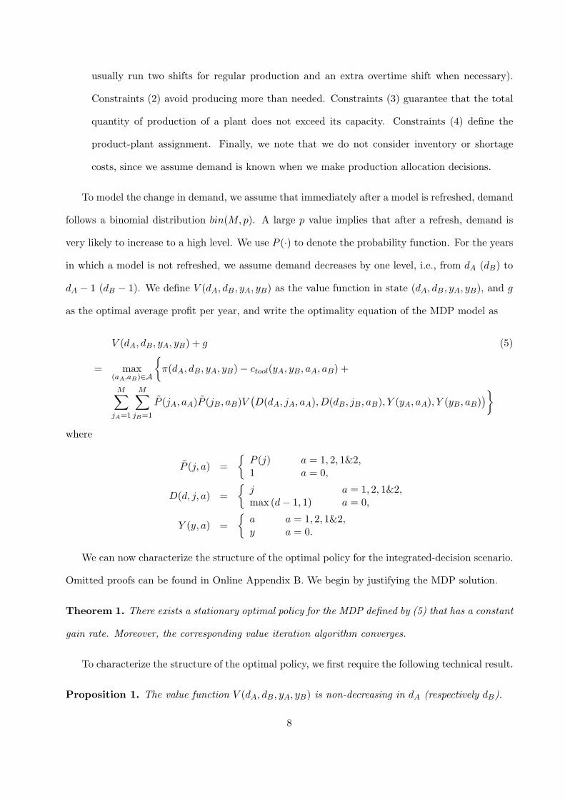
as the optimal average profit per year, and write the optimality equation of the MDP model as

V (dA, dB, yA, yB) + g (5)

= max(aA,aB)∈A

{π(dA, dB, yA, yB)− ctool(yA, yB, aA, aB) +

M∑

jA=1

M∑

jB=1

P̃ (jA, aA)P̃ (jB, aB)V(D(dA, jA, aA), D(dB, jB, aB), Y (yA, aA), Y (yB, aB)

)}

where

P̃ (j, a) ={

P (j) a = 1, 2, 1&2,1 a = 0,

D(d, j, a) ={

j a = 1, 2, 1&2,max (d− 1, 1) a = 0,

Y (y, a) ={

a a = 1, 2, 1&2,y a = 0.

We can now characterize the structure of the optimal policy for the integrated-decision scenario.

Omitted proofs can be found in Online Appendix B. We begin by justifying the MDP solution.

Theorem 1. There exists a stationary optimal policy for the MDP defined by (5) that has a constant

gain rate. Moreover, the corresponding value iteration algorithm converges.

To characterize the structure of the optimal policy, we first require the following technical result.

Proposition 1. The value function V (dA, dB, yA, yB) is non-decreasing in dA (respectively dB).

8

Now we present the main result of the subsection.

Theorem 2. If the action “no refresh for product A (respectively B)” is optimal for state (dA, dB, yA, yB),

then it is optimal for state (dA + 1, dB, yA, yB) (respectively (dA, dB + 1, yA, yB)) for all 1 ≤ dA ≤

M − 1 (respectively 1 ≤ dB ≤ M − 1).

Theorem 2 says that the optimal policy follows a one-dimensional threshold structure in demand

level. As we show in Appendix B, that Theorem 2 holds for an N -product K-plant system and

general probability function P (·), not just the 2-product 2-plant system and binomial distribution.

2.2 MDP Formulation for a 2-Product 2-Plant System: Decoupled Decisions

When portfolio and plant assignment decisions are made separately, portfolio decision makers may

look at historical data to get an idea of how much it will cost to retool a factory for a new model,

even though they do not know the specific factory that will be retooled. We model the decoupled

decision making case as a three-stage process. First, average net revenue and tooling costs are

estimated assuming a fixed refresh cycle; this imitates the real process of using historical data

to obtain averages. To be conservative in our comparison of integrated and decoupled decision

making we make the process as favorable as possible for the decoupled case by getting good average

numbers for net revenue and tooling costs. In practice, such numbers would be estimated from

historical averages. But here we solve an off-line MDP with fixed refresh cycle length for optimal

plant assignment and production allocation, and compute average tooling costs under the optimal

policy. Then, the portfolio decisions are made using the average net revenue and costs from this

computation. Finally, we solve the plant assignment problem as an MDP with a restricted action

space determined by the portfolio decisions. We describe this three-stage process in detail in Online

Appendix A. We can demonstrate similar results to those of Theorem 1 for the MDP of each stage,

which we state as Theorem 3 in Online Appendix A.

3 Numerical Results

In this section we assess the value of integrating the portfolio planning and plant assignment decisions

by means of a numerical study. We use value iteration to find the optimal policy for both the

9

������� �������� � ��� ���� ����������������������������������� �������� �������� �������� �

������� �������� �������� �������� �������� �������� �

(a)

(c)

(b)

��� ��� ��� ��� ��� ��� ���� � ��� ���� � ��� �������������������� �������� � ������� �������� �(d)

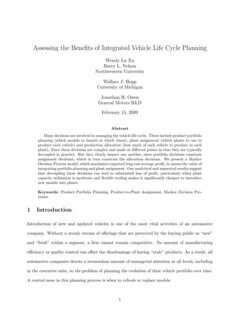
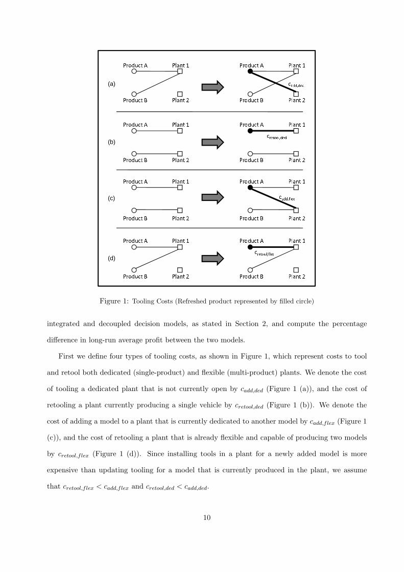
��� ��� ��� � ��� �Figure 1: Tooling Costs (Refreshed product represented by filled circle)

integrated and decoupled decision models, as stated in Section 2, and compute the percentage

difference in long-run average profit between the two models.

First we define four types of tooling costs, as shown in Figure 1, which represent costs to tool

and retool both dedicated (single-product) and flexible (multi-product) plants. We denote the cost

of tooling a dedicated plant that is not currently open by cadd,ded (Figure 1 (a)), and the cost of

retooling a plant currently producing a single vehicle by cretool,ded (Figure 1 (b)). We denote the

cost of adding a model to a plant that is currently dedicated to another model by cadd,flex (Figure 1

(c)), and the cost of retooling a plant that is already flexible and capable of producing two models

by cretool,flex (Figure 1 (d)). Since installing tools in a plant for a newly added model is more

expensive than updating tooling for a model that is currently produced in the plant, we assume

that cretool,flex < cadd,flex and cretool,ded < cadd,ded.

10

To limit our consideration to realistic cost scenarios, note that the cost of retooling consists

of model-level and plant-level costs. Plant-level costs (e.g., power supply, ventilation, material

handling) serve all models that are produced in the plant. Model-level costs are specific to the

models produced (e.g., tooling for pressing sheet metal). When a model is retooled, we update both

the model and plant, and hence incur both costs. When a plant produces multiple models, the plant-

level costs are apportioned to the various models. Therefore, the total cost of retooling ALL models

in a plant producing multiple models will be more expensive than retooling one model in a dedicated

plant (because of the additional model-specific cost). This implies that 2cretool,flex > cretool,ded.

However, retooling ONE model in a multiple-model plant is less expensive than retooling one model

in a single-model dedicated plant (because we are only paying part of the plant-level costs). This

means that cretool,flex < cretool,ded.

Of course, the cost of opening an empty plant to produce one model incurs both model-level and

plant-level costs; while installing tools in a plant that currently produces only one model so that it

can also produce a second model incurs primarily model-level costs (because plant-level tooling is

already there and can be shared). This implies that cadd,flex < cadd,ded.

Finally, to reduce the number of parameters we need to vary, and to simplify the analysis,

we assume that cadd,ded/cretool,ded = cadd,flex/cretool,flex, and therefore we have cadd,ded/cadd,flex =

cretool,ded/cretool,flex. Our solution methodology does not require these conditions, however. We let

ctotal = cadd,ded + cadd,flex + cretool,ded + cflex,ded.

We can now state the following proposition:

Proposition 2. If a 2-product 2-plant system is symmetric, i.e., mA = mB , m, cOT,1 = cOT,2 ,

cOT , and Kreg,1 = Kreg,2 , Kreg, then for a given demand value function f(·) the system can be

fully described by the following five parameters, in the sense that the optimal policy for integrated

and decoupled decisions, as well as the percentage difference in long-run average profit between the

integrated and decoupled decision models, is solely determined by these five parameters:

1. Dedicated-to-flexible cost ratio = cadd,ded/cadd,flex = cretool,ded/cretool,flex;

2. Tool-to-retool cost ratio = cadd,ded/cretool,ded = cadd,flex/cretool,flex;

11

3. Margin-normalized overtime cost = cOT /m;

4. Utilization = f(M)/Kreg;

5. Tooling-cost-to-revenue factor = ctotal/(m ∗Kreg).

Proposition 2 allows us to normalize all the system parameters, which generalizes our analysis

beyond the specific cases considered in our numerical study.

To keep computation reasonable, we set the number of demand levels to M = 5. We use

demand value function f(d) = 0.2d to reflect a 20% annual decrease in demand. We use p = 0.9 for

the binomial distribution of first-year demand, so that after a model refresh, demand rises to the

maximum level with about 0.65 probability and reaches 80% of the maximum with 0.95 probability.

We vary the five parameters to cover the region of practical interest as follows:

1. Dedicated-to-flexible cost ratio 1 ≤ cadd,ded/cadd,flex = cretool,ded/cretool,flex ≤ 2;

2. Tool-to-retool cost ratio 1 ≤ cadd,ded/cretool,ded = cadd,flex/cretool,flex ≤ 2;

3. Margin-normalized overtime cost 0.05 ≤ cOT /m ≤ 0.5;

4. Utilization 0.5 ≤ f(M)/Kreg ≤ 5;

5. Tooling-cost-to-revenue factor 2 ≤ ctotal/(m ∗Kreg) ≤ 20.

By examining the results of these numerical cases, we made the following observations:

OBSERVATION 1. Integrated decision making typically outperforms decoupled decision mak-

ing, although there are certain parameter sets under which the decoupled decision achieves the same

performance as the integrated decision (this occurs when the estimates of tooling costs and net rev-

enue happen to be correct). Decoupled decision making cannot outperform integrated decision

making, so the smallest percentage difference is zero.

OBSERVATION 2. The parameters “tool-to-retool cost ratio” and “margin-normalized overtime

cost” do not have a significant effect on relative performance of the two systems. Therefore, from

here on we fix the tool-to-retool cost ratio at 1.8 and the margin-normalized overtime cost at 0.2 to

simplify analysis.

12

The intuition behind observation 2 is that, while “tool-to-retool cost ratio” and “margin-

normalized overtime cost” do affect the expected profit, their impact does not depend on whether or

not the portfolio planning and plant assignment are integrated. In the former case, this is because

“tool-to-retool cost ratio” affects the optimal pace of refreshment similarly in both the integrated

and decoupled settings. In the latter case, the “margin-normalized overtime cost” affects the cost of

production, and hence the optimal loading of plants, which affects decision making in the integrated

and decoupled cases similarly.

We now examine the effect of utilization and dedicated-to-flexible cost ratio on the value of

integrating decisions. To do this, we introduce a “statistical” approach for analyzing data. The

reason this is needed is that, as we noted earlier, the decoupled decision can often result in the

same actions, and hence the same profit, as the integrated decision. So looking at the average profit

across a range of cases does not fully characterize the difference between the two approaches. To

better reveal this difference, we report multiple percentiles, as opposed to only the mean.

To illustrate this, we consider the impact of utilization on expected profit. With the tool-to-

retool cost ratio and margin-normalized overtime cost fixed, we vary the dedicated-to-flexible cost

ratio and tooling-cost-to-revenue factor over the ranges given above and calculate the percentage

difference between the long-run average profits under optimal integrated and optimal decoupled

decision making. Over all the cases, those for which which integrated decision making outperforms

decoupled decision making by the largest amounts are of particular interest. So, to see these,

we sort the percentage differences, and use the y quantile to measure the performance of the top

100(1− y) percent of the cases. If the y quantile for the utilization value u1 is larger than that for

the utilization value u2, then we conclude that the performance advantage of integrated decision

making over decoupled decision making is larger when utilization is u1 than when it is u2 for the top

100(1− y) percent of cases. By looking at multiple percentiles, we can get a sense of how likely and

how large the increase in profits will be by using integrated decision making in place of decoupled

decision making.

With this definition of a performance improvement in mind, we can now state our observations

about the impact of utilization and dedicated-to-flexible cost ratio on the value of integration.

13

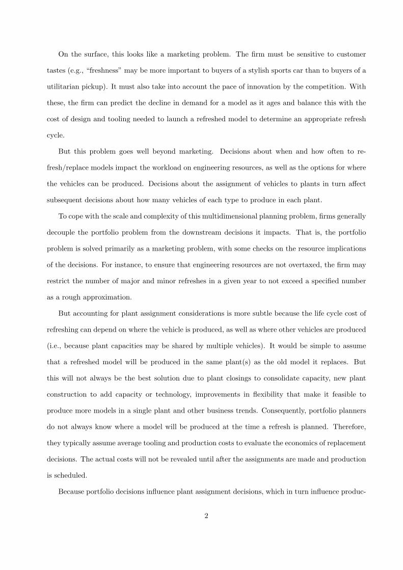
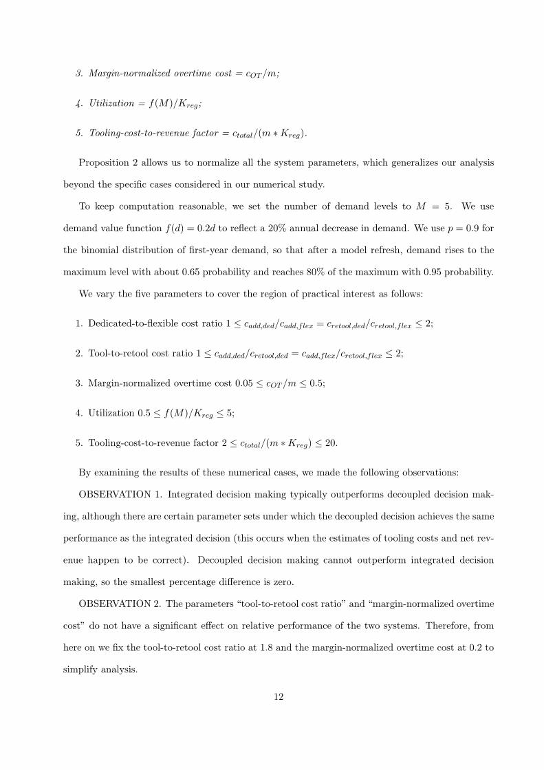
OBSERVATION 3. The value of integrating portfolio and plant assignment decisions is largest

when the system is not over-capacitated or under-capacitated, as shown in Figure 2, where we vary

utilization from 0.5 to 5 with step size 0.1. For each utilization value, we also vary the dedicated-

to-flexible cost ratio from 1.1 to 1.7 with step size 0.1, and tooling-cost-to-revenue factor from 2 to

20 with step size 0.2. For each utilization this gives about 650 cases whose percentage differences

are sorted. We depict the y quantile of percentage difference with y values 0.5, 0.7, 0.9 and 1.

We can see from Figure 2 that the value of integrating portfolio and plant assignment decisions

is maximized when utilization is around 1.5. Since utilization is defined as maximum demand over

regular capacity, a utilization of 1.5 means total maximum demand equals total capacity in the

system. When the system is over-capacitated, say with utilization smaller than 0.8, in 90% out of

650 cases the integrated decision outperforms the decoupled decision by less than 2%, so the value

of integrating portfolio planning and plant allocation is not likely to be large. In contrast, when

the system is under-capacitated, say with utilization larger than 4.5, in 90% out of 650 cases the

integrated decision outperforms the decoupled decision by less than 3%, and in 70% out of 650 cases

the integrated and decoupled decision systems perform about the same, so the value of integrating

the two decisions is not large in this case either.

This observation is potentially of great practical significance, since it implies that integrating

portfolio planning and plant assignment decisions is most important precisely when capacity is fully

utilized. Since firms are likely to make capacity decisions over the long term that push utilization

near this point, this suggests that integrating these two decisions could substantially improve profits

in practice.

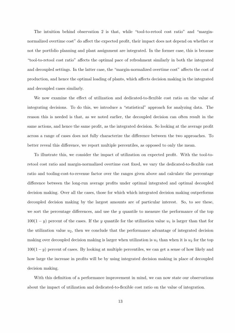
OBSERVATION 4. As the dedicated-to-flexible cost ratio increases, the value of integrating port-

folio and plant assignment decisions increases, as shown in Figure 3, where we vary the dedicated-

to-flexible cost ratio from 1.1 to 1.7 with step size 0.1. For each ratio, we also vary the utilization

from 0.5 to 5 with step size 0.1, and tooling-cost-to-revenue factor from 2 to 20 with step size 0.2.

Therefore for each dedicated-to-flexible cost ratio we have about 4, 000 cases. We depict the y quan-

tile curve of percentage difference for y = 0.95, 0.99, 1.0. Note that only the 1.0 quantile (i.e., the

maximum value) is strictly increasing in the dedicated-to-flexible cost ratio. In fact, our data show

14

�������������� �� ��� ������ ������� ������ � ���� ����� ������

0.5 1 1.5 2 2.5 3 3.5 4 4.5 50

10

20

30

40

50

60

70

0.5

0.70.9

1

Figure 2: Effect of Utilization on the Value of Integrating Decisions

������������������ �� � ������������� ��� �������������� ������ � � �� ��!��� �����"1.1 1.2 1.3 1.4 1.5 1.6 1.7 1.80

10

20

30

40

50

60

70

0.95

0.991

Figure 3: Effect of Dedicated-to-Flexible Cost Ratio

that any quantile above the 0.99 quantile is monotonically increasing. This means that if we focus

on any percentage less than 1% of the 4, 000 cases with the largest differences between integrated

and decoupled decisions, the value of incorporating the impact of current portfolio decisions on

later-stage planning decisions increases as the dedicated-to-flexible cost ratio increases. The 0.95

and 0.99 percentiles are not strictly increasing, but still show an overall increasing trend in the

dedicated-to-flexible cost ratio.

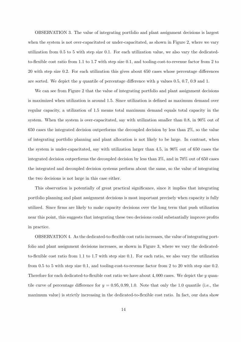
We can explain the intuition behind this observation by examining the optimal policies more

closely. To do this, we define the following two steady-state measures under optimal integrated

and decoupled decision policies: (i) average number of plants that are in use, which we call average

15

���� � ��� �� ������ �� 0.8

1

������ ��� ���� ���� �� �� ��� �� ��� �� � 0.2

0.4

0.6

�� � �� ��� ����� � ��� ����� �� ��1.1 1.2 1.3 1.4 1.5 1.6 1.7 1.8

-0.4

-0.2

0

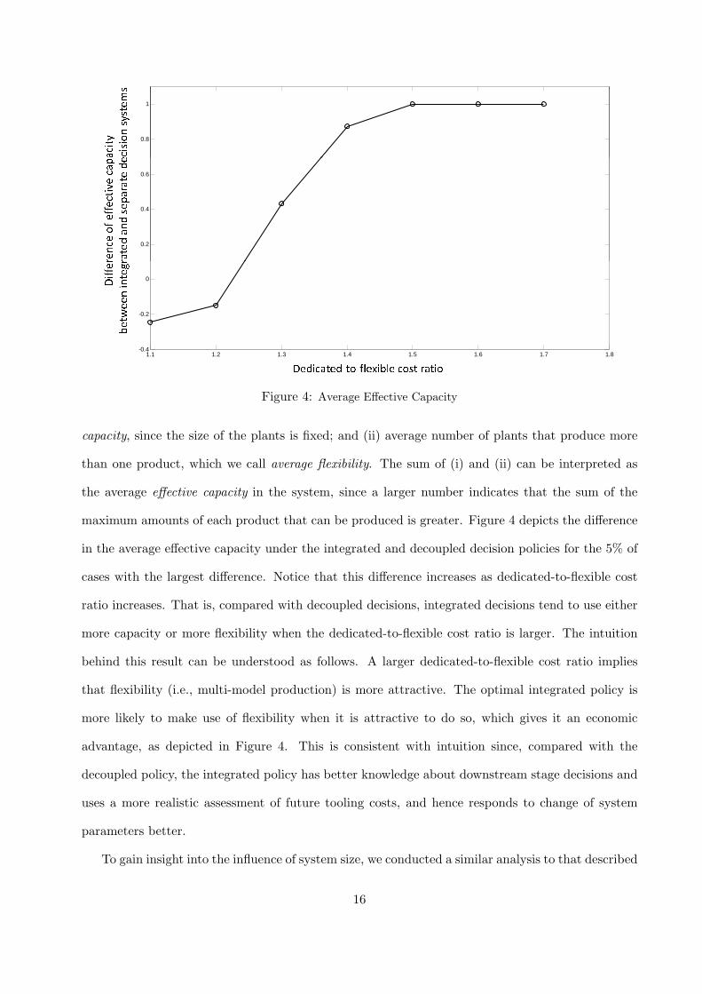
� � ���� �� ���� ���� ����� �� � !� ���Figure 4: Average Effective Capacity

capacity, since the size of the plants is fixed; and (ii) average number of plants that produce more

than one product, which we call average flexibility. The sum of (i) and (ii) can be interpreted as

the average effective capacity in the system, since a larger number indicates that the sum of the

maximum amounts of each product that can be produced is greater. Figure 4 depicts the difference

in the average effective capacity under the integrated and decoupled decision policies for the 5% of

cases with the largest difference. Notice that this difference increases as dedicated-to-flexible cost

ratio increases. That is, compared with decoupled decisions, integrated decisions tend to use either

more capacity or more flexibility when the dedicated-to-flexible cost ratio is larger. The intuition

behind this result can be understood as follows. A larger dedicated-to-flexible cost ratio implies

that flexibility (i.e., multi-model production) is more attractive. The optimal integrated policy is

more likely to make use of flexibility when it is attractive to do so, which gives it an economic

advantage, as depicted in Figure 4. This is consistent with intuition since, compared with the

decoupled policy, the integrated policy has better knowledge about downstream stage decisions and

uses a more realistic assessment of future tooling costs, and hence responds to change of system

parameters better.

To gain insight into the influence of system size, we conducted a similar analysis to that described

16

������������������ �� � ������������� ��� �������������� ������ � � �� ��!��� �����"1.1 1.2 1.3 1.4 1.5 1.6 1.7 1.85

10

15

20

25

30

35

40

0.95

0.991

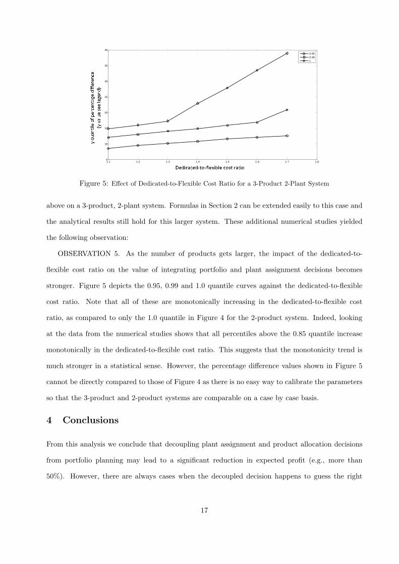
Figure 5: Effect of Dedicated-to-Flexible Cost Ratio for a 3-Product 2-Plant System

above on a 3-product, 2-plant system. Formulas in Section 2 can be extended easily to this case and

the analytical results still hold for this larger system. These additional numerical studies yielded

the following observation:

OBSERVATION 5. As the number of products gets larger, the impact of the dedicated-to-

flexible cost ratio on the value of integrating portfolio and plant assignment decisions becomes

stronger. Figure 5 depicts the 0.95, 0.99 and 1.0 quantile curves against the dedicated-to-flexible

cost ratio. Note that all of these are monotonically increasing in the dedicated-to-flexible cost

ratio, as compared to only the 1.0 quantile in Figure 4 for the 2-product system. Indeed, looking

at the data from the numerical studies shows that all percentiles above the 0.85 quantile increase

monotonically in the dedicated-to-flexible cost ratio. This suggests that the monotonicity trend is

much stronger in a statistical sense. However, the percentage difference values shown in Figure 5

cannot be directly compared to those of Figure 4 as there is no easy way to calibrate the parameters

so that the 3-product and 2-product systems are comparable on a case by case basis.

4 Conclusions

From this analysis we conclude that decoupling plant assignment and product allocation decisions

from portfolio planning may lead to a significant reduction in expected profit (e.g., more than

50%). However, there are always cases when the decoupled decision happens to guess the right

17

downstream cost and match the integrated solution. But because we cannot predict when this will

occur, our study focuses on the conditions under which the risk of a bad decision from using a

decoupled model is large. Our numerical results show that this risk of a large profit penalty from

using a decoupled model to address the portfolio planning problem is greatest when plant capacity

utilization is moderate and flexible tooling makes it significantly cheaper to introduce new models

into plants.

Using an exact optimization model to integrate portfolio planning and plant assignment deci-

sions, as we have done in this paper, is only feasible for very small systems. For realistically sized

problems it may be necessary to use a simulation-based optimization model to efficiently search over

all possible decisions. However, it may be effective to decouple the problem by segments and use

an analytic model like that developed here to optimize each segment for a given resource allocation

(e.g., of engineering resources, marketing resources, or vehicle launches). Developing a modeling

platform with which to search for the optimal resource allocation is the logical next step toward a

practical tool for integrated product portfolio and plant allocation planning.

References

Alden J. M., T. Costy and R. R. Inman (2002). Product-to-plant allocation assessment in the automotiveindustry. Journal of Manufacturing Systems 21, 1, 1-13.

Barlow, R. E., F. Proschan and L. C. Hunter (1965). Mathematical Theory of Reliability John Wiley &Sons, New York.

Cooper, R. G., S. J. Edgett and E. J. Kleinschmidt (1999). New product potfolio management: practiceand performance. J. Prod. Innov. Manag. 16, 333-351.

Dickinson, M. W., A. C. Thornton and S. Graves (2001). Technology Portfolio Management: Optimizinginterdependent projects over multiple time periods. IEEE Transaction on Engineering ManagementVol. 48, No. 4, 518-527.

Heidenberger, K. and C. Stummer (1999). Research and development project selection and resource alloca-tion: A review of quatitative modeling approaches. Intl. J. Manag. Rev. Vol. 1, 197-224.

Inman, R. R. and D. J. A. Gonsalvez (2001). A mass production product-to-plant allocation problem.Computers and Industrial Engineering 39, 255-271.

Loch, C. H. and S. Kavadias (2002). Dynamic portfolio selection of NPD programs using marginal returns.Management Science Vol. 48, No. 10, 1227-1241.

McCall, J. J. (1965). Maintenance policies for stochastically failing equipment: a survey. ManagementScience 11, 5, 493-524.

Pierskalla, W. P. and J. A. Voelker (1976). A survey of maintenance models: the control and surveillanceof deteriorating systems. Naval Research Logistics Quarterly 23, 3, 353-388.

18

Puterman, M. L. (1994). Markov Decision Process. Wiley, New York.

Sherif, Y. S. and M. L. Smith (1981). Optimal maintenance models for systems subject to failure - a review.Naval Research Logistics Quarterly 28, 1, 47-74.

Sloan, T. W. and J. G. Shanthikumar (2000). Combined production and maintenance scheduling for amulti-product single-machine production system. Prodection and Operations Management 9, 4, 379-399.

Stummer, C. and K. Heidensberger (2003). Interactive R& D portfolio analysis with project interdependen-cies and time profiles of multiple objectives. IEEE Transaction on Engineering Management Vol. 50,No. 2, 175-183.

Valdez-Flores, C. and R. M. Feldman (1989). A survey of preventive maintenance models for stochasticallydeteriorating single-unit systems. Naval Research Logistics 36, 419-446.

Wang, H. (2002). A survey of maintenance policies of deteriorating systems. European Journal of Opera-tional Research 139, 469-489.

19

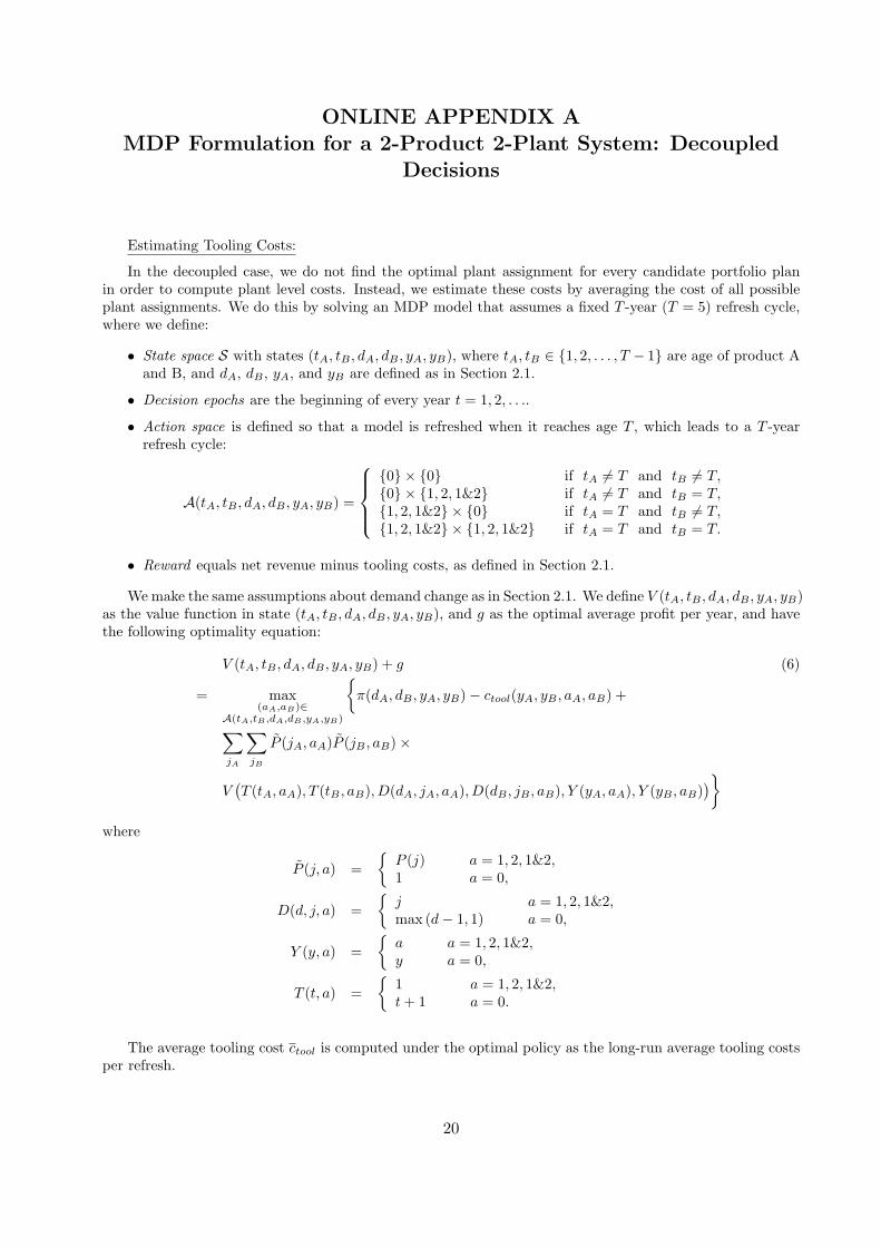
ONLINE APPENDIX AMDP Formulation for a 2-Product 2-Plant System: Decoupled

Decisions

Estimating Tooling Costs:

In the decoupled case, we do not find the optimal plant assignment for every candidate portfolio planin order to compute plant level costs. Instead, we estimate these costs by averaging the cost of all possibleplant assignments. We do this by solving an MDP model that assumes a fixed T -year (T = 5) refresh cycle,where we define:

• State space S with states (tA, tB , dA, dB , yA, yB), where tA, tB ∈ {1, 2, . . . , T − 1} are age of product Aand B, and dA, dB , yA, and yB are defined as in Section 2.1.

• Decision epochs are the beginning of every year t = 1, 2, . . ..

• Action space is defined so that a model is refreshed when it reaches age T , which leads to a T -yearrefresh cycle:

A(tA, tB , dA, dB , yA, yB) =

{0} × {0} if tA 6= T and tB 6= T,{0} × {1, 2, 1&2} if tA 6= T and tB = T,{1, 2, 1&2} × {0} if tA = T and tB 6= T,{1, 2, 1&2} × {1, 2, 1&2} if tA = T and tB = T.

• Reward equals net revenue minus tooling costs, as defined in Section 2.1.

We make the same assumptions about demand change as in Section 2.1. We define V (tA, tB , dA, dB , yA, yB)as the value function in state (tA, tB , dA, dB , yA, yB), and g as the optimal average profit per year, and havethe following optimality equation:

V (tA, tB , dA, dB , yA, yB) + g (6)

= max(aA,aB)∈

A(tA,tB ,dA,dB ,yA,yB)

{π(dA, dB , yA, yB)− ctool(yA, yB , aA, aB) +

∑

jA

∑

jB

P̃ (jA, aA)P̃ (jB , aB)×

V(T (tA, aA), T (tB , aB), D(dA, jA, aA), D(dB , jB , aB), Y (yA, aA), Y (yB , aB)

)}

where

P̃ (j, a) ={

P (j) a = 1, 2, 1&2,1 a = 0,

D(d, j, a) ={

j a = 1, 2, 1&2,max (d− 1, 1) a = 0,

Y (y, a) ={

a a = 1, 2, 1&2,y a = 0,

T (t, a) ={

1 a = 1, 2, 1&2,t + 1 a = 0.

The average tooling cost ctool is computed under the optimal policy as the long-run average tooling costsper refresh.

20

For the net revenue, we compute the average of all possible plan assignments for each demand level:

π(dA, dB) =19

∑yA

∑yB

π(dA, dB , yA, yB).

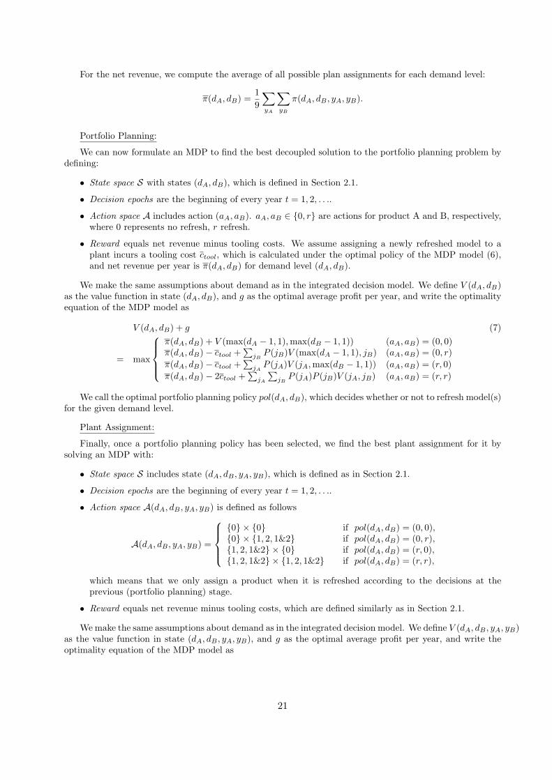
Portfolio Planning:

We can now formulate an MDP to find the best decoupled solution to the portfolio planning problem bydefining:

• State space S with states (dA, dB), which is defined in Section 2.1.

• Decision epochs are the beginning of every year t = 1, 2, . . ..

• Action space A includes action (aA, aB). aA, aB ∈ {0, r} are actions for product A and B, respectively,where 0 represents no refresh, r refresh.

• Reward equals net revenue minus tooling costs. We assume assigning a newly refreshed model to aplant incurs a tooling cost ctool, which is calculated under the optimal policy of the MDP model (6),and net revenue per year is π(dA, dB) for demand level (dA, dB).

We make the same assumptions about demand as in the integrated decision model. We define V (dA, dB)as the value function in state (dA, dB), and g as the optimal average profit per year, and write the optimalityequation of the MDP model as

V (dA, dB) + g (7)

= max

π(dA, dB) + V (max(dA − 1, 1), max(dB − 1, 1)) (aA, aB) = (0, 0)π(dA, dB)− ctool +

∑jB

P (jB)V (max(dA − 1, 1), jB) (aA, aB) = (0, r)π(dA, dB)− ctool +

∑jA

P (jA)V (jA,max(dB − 1, 1)) (aA, aB) = (r, 0)π(dA, dB)− 2ctool +

∑jA

∑jB

P (jA)P (jB)V (jA, jB) (aA, aB) = (r, r)

We call the optimal portfolio planning policy pol(dA, dB), which decides whether or not to refresh model(s)for the given demand level.

Plant Assignment:

Finally, once a portfolio planning policy has been selected, we find the best plant assignment for it bysolving an MDP with:

• State space S includes state (dA, dB , yA, yB), which is defined as in Section 2.1.

• Decision epochs are the beginning of every year t = 1, 2, . . ..

• Action space A(dA, dB , yA, yB) is defined as follows

A(dA, dB , yA, yB) =

{0} × {0} if pol(dA, dB) = (0, 0),{0} × {1, 2, 1&2} if pol(dA, dB) = (0, r),{1, 2, 1&2} × {0} if pol(dA, dB) = (r, 0),{1, 2, 1&2} × {1, 2, 1&2} if pol(dA, dB) = (r, r),

which means that we only assign a product when it is refreshed according to the decisions at theprevious (portfolio planning) stage.

• Reward equals net revenue minus tooling costs, which are defined similarly as in Section 2.1.

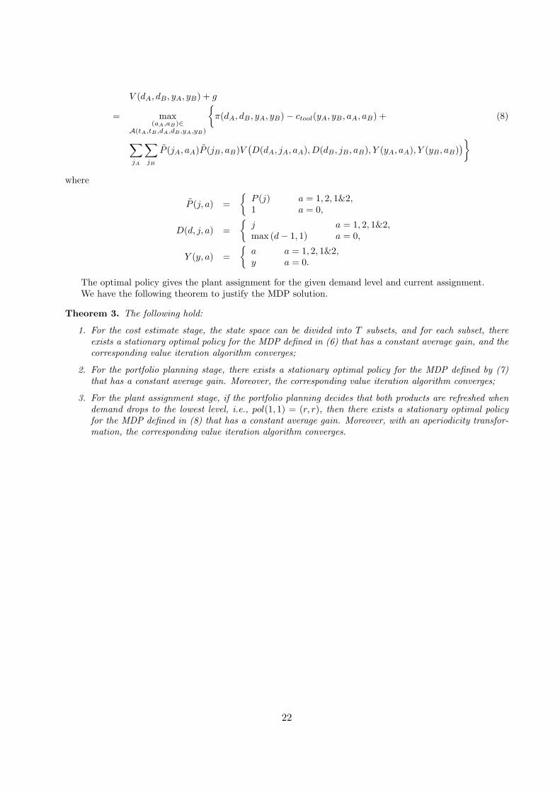
We make the same assumptions about demand as in the integrated decision model. We define V (dA, dB , yA, yB)as the value function in state (dA, dB , yA, yB), and g as the optimal average profit per year, and write theoptimality equation of the MDP model as

21

V (dA, dB , yA, yB) + g

= max(aA,aB)∈

A(tA,tB ,dA,dB ,yA,yB)

{π(dA, dB , yA, yB)− ctool(yA, yB , aA, aB) + (8)

∑

jA

∑

jB

P̃ (jA, aA)P̃ (jB , aB)V(D(dA, jA, aA), D(dB , jB , aB), Y (yA, aA), Y (yB , aB)

)}

where

P̃ (j, a) ={

P (j) a = 1, 2, 1&2,1 a = 0,

D(d, j, a) ={

j a = 1, 2, 1&2,max (d− 1, 1) a = 0,

Y (y, a) ={

a a = 1, 2, 1&2,y a = 0.

The optimal policy gives the plant assignment for the given demand level and current assignment.We have the following theorem to justify the MDP solution.

Theorem 3. The following hold:

1. For the cost estimate stage, the state space can be divided into T subsets, and for each subset, thereexists a stationary optimal policy for the MDP defined in (6) that has a constant average gain, and thecorresponding value iteration algorithm converges;

2. For the portfolio planning stage, there exists a stationary optimal policy for the MDP defined by (7)that has a constant average gain. Moreover, the corresponding value iteration algorithm converges;

3. For the plant assignment stage, if the portfolio planning decides that both products are refreshed whendemand drops to the lowest level, i.e., pol(1, 1) = (r, r), then there exists a stationary optimal policyfor the MDP defined in (8) that has a constant average gain. Moreover, with an aperiodicity transfor-mation, the corresponding value iteration algorithm converges.

22

ONLINE APPENDIX BProofs of Analytical Results

PROOF OF THEOREM 1:

Since state space S and action set A are finite, by Theorem 9.1.8 of Puterman (1994), there exists a deter-ministic stationary optimal policy.

We now prove that the model is communicating. For an arbitrary pair of states s = (dA, dB , yA, yB) ands′ = (d′A, d′B , y′A, y′B), under action a = (y′A, y′B), state s reaches state s′ with probability P (d′A)P (d′B) > 0(from the property of binomial distribution probability function). Therefore, s′ is accessible from s under astationary deterministic policy d∞ with d(s) = (y′A, y′B). Since s and s′ are arbitrarily chosen, this completesthe proof. Hence, by Theorem 8.3.2 of Puterman (1994), there exists a stationary optimal policy with constantgain.

From Section 8.5.4 of Puterman (1994), we know that through a simple transformation, all policies canbe made aperiodic. Then by Corollary 9.4.6 of Puterman (1994), the value iteration algorithm converges andthe span can be used as a stopping criterion.

PROOF OF PROPOSITION 1:

We use induction and value iteration to prove the proposition.It is clear that at the first iteration of the value iteration algorithm, V0(dA, dB , yA, yB) = π(dA, dB , yA, yB)

is non-decreasing in dA. We assume that value function is non-decreasing in dA at iteration k, we will provethat it is non-decreasing in dA at iteration k + 1.

Vk+1(dA, dB , yA, yB) (9)

= max(aA,aB)∈A

{π(dA, dB , yA, yB)− ctool(yA, yB , aA, aB) +

∑

jA

∑

jB

P̃ (jA, aA)P̃ (jB , aB)Vk

(D(dA, jA, aA), D(dB , jB , aB), Y (yA, aA), Y (yB , aB)

)}

where

P̃ (j, a) ={

P (j) a = 1, 2, 1&2,1 a = 0,

D(d, j, a) ={

j a = 1, 2, 1&2,max (d− 1, 1) a = 0,

Y (y, a) ={

a a = 1, 2, 1&2,y a = 0.

Since π(dA, dB , yA, yB) is non-decreasing in dA, ctool(yA, yB , aA, aB) does not depend on dA, D(d, j, a)is non-decreasing in d and Vk(dA, dB , yA, yB) is non-decreasing in dA, the expression within braces in (9) isnon-decreasing in dA. Therefore Vk+1(dA, dB , yA, yB) is non-decreasing in dA.

PROOF OF THEOREM 2:

Define

R(dA, dB , yA, yB , aA, aB)= π(dA, dB , yA, yB)− ctool(yA, yB , aA, aB) +∑

jA

∑

jB

P̃ (jA, aA)P̃ (jB , aB)Vk

(D(dA, jA, aA), D(dB , jB , aB), Y (yA, aA), Y (yB , aB)

),

23

where

P̃ (j, a) ={

P (j) a = 1, 2, 1&2,1 a = 0,

D(d, j, a) ={

j a = 1, 2, 1&2,max (d− 1, 1) a = 0,

Y (y, a) ={

a a = 1, 2, 1&2,y a = 0.

Suppose action (0, β) is optimal at state (dA, dB , yA, yB) for some β ∈ {0, 1, 2, 1&2}, we have

R(dA, dB , yA, yB , 0, β) ≥ R(dA, dB , yA, yB , aA, aB) ∀ aA ∈ {1, 2, 1&2}, aB ∈ {0, 1, 2, 1&2}. (10)

We will prove (0, β) dominates all the “refresh for model A” actions at state (dA + 1, dB , yA, yB), i.e.,

R(dA + 1, dB , yA, yB , 0, β) ≥ R(dA + 1, dB , yA, yB , aA, aB) ∀ aA ∈ {1, 2, 1&2}, aB ∈ {0, 1, 2, 1&2}. (11)

From the optimality Equation (5) we have

R(dA + 1, dB , yA, yB , 0, 0)−R(dA, dB , yA, yB , 0, 0)= π(dA + 1, dB , yA, yB)− π(dA, dB , yA, yB)

+ V (max(dA, 1), max(dB − 1, 1), yA, yB)− V (max(dA − 1, 1), max(dB − 1, 1), yA, yB),

and for all aB ∈ {1, 2, 1&2},

R(dA + 1, dB , yA, yB , 0, aB)−R(dA, dB , yA, yB , 0, aB)= π(dA + 1, dB , yA, yB)− π(dA, dB , yA, yB)

+∑

jB

P (jB)V (max(dA, 1), jB , yA, aB)−∑

jB

P (jB)V (max(dA − 1, 1), jB , yA, aB).

From Proposition 1, V (dA, dB , yA, yB) is non-decreasing in dA. Also, max(dA− 1, 1) is non-decreasing in dA.Therefore for aB ∈ {0, 1, 2, 1&2}, we have

R(dA + 1, dB , yA, yB , 0, aB)−R(dA, dB , yA, yB , 0, aB) ≥ π(dA + 1, dB , yA, yB)− π(dA, dB , yA, yB). (12)

On the other hand, for aA ∈ {1, 2, 1&2}, since dA appears in R(dA, dB , yA, yB , aA, aB) only through π(·), wehave

R(dA + 1, dB , yA, yB , aA, aB)−R(dA, dB , yA, yB , aA, aB) = π(dA + 1, dB , yA, yB)− π(dA, dB , yA, yB)∀ aA ∈ {1, 2, 1&2}, aB ∈ {0, 1, 2, 1&2}. (13)

Therefore,

R(dA + 1, dB , yA, yB , 0, β)−R(dA, dB , yA, yB , 0, β)≥ π(dA + 1, dB , yA, yB)− π(dA, dB , yA, yB) from (12)= R(dA + 1, dB , yA, yB , aA, aB)−R(dA, dB , yA, yB , aA, aB) from (13)

∀ aA ∈ {1, 2, 1&2}, aB ∈ {0, 1, 2, 1&2},

or equivalently,

R(dA + 1, dB , yA, yB , 0, β)−R(dA + 1, dB , yA, yB , aA, aB)≥ R(dA, dB , yA, yB , 0, β)−R(dA, dB , yA, yB , aA, aB)≥ 0 from (10)

∀ aA ∈ {1, 2, 1&2}, aB ∈ {0, 1, 2, 1&2},

and (11) follows.

24

Note that the proof of Theorem 2 does not depend on the size of the system. It does require thatP (M) 6= 0 so the MDP is weakly communicating. Theorem 2 holds for an N -product K-plant system andgeneral probability function, as long as P (M) 6= 0.

PROOF OF THEOREM 3:

PART 1

First we divide the state space S into T subsets S = S0 ∪ S1 ∪ · · · ∪ ST−1, where

(tA, tB , dA, dB , yA, yB) ∈

S0 if (tA, tB) ∈ {(1, 1), (2, 2), . . . , (T, T )}S1 if (tA, tB) ∈ {(1, 2), (2, 3), . . . , (T, 1)}...ST−1 if (tA, tB) ∈ {(1, T ), (2, 1), . . . , (T, T − 1)}.

(14)

We focus on one subset Sk (k ∈ {0, 1, . . . , T − 1}). Since state space Sk and action set A are finite, byTheorem 9.1.8 of Puterman (1994), there exists a deterministic stationary optimal policy.

Now we prove that the MDP defined by (6) is weakly communicating. We know that all the states withtA + dA − 1 > T or tB + dB − 1 > T are transient since they are not reachable from any other states underall policies. For an arbitrary pair of states s = (tA, tB , dA, dB , yA, yB) and s′ = (t′A, t′B , d′A, d′B , y′A, y′B) thatare not transient, define ∆tA = t′A − tA and ∆tB = t′B − tB . From the way Sk is defined in (14), we haveeither ∆tA = ∆tB or |∆tA −∆tB | = T .

For the ∆tA = ∆tB case, define ∆t , ∆tA = ∆tB . Consider a ∆t-step transition from state s, whichupdates the age of the two products from (tA, tB) to (t′A, t′B). Within these steps both product A and B arerefreshed exactly once. Choose action y′A when product A is refreshed, and choose action y′B when productB is refreshed. Then with probability P (d′A + t′A − 1)P (d′B + t′B − 1) > 0, state s′ is reached.

For the |∆tA − ∆tB | = T case, without loss of generality, assume tA > 0. Consider a (T + ∆tA)-steptransition from state s, which updates the age of the two products from (tA, tB) to (t′A, t′B). Within thesesteps product A is refreshed twice and product B is refreshed once. Choose action y′A when product Ais refreshed the second time, and choose action y′B when product B is refreshed. Then with probabilityP (d′A + t′A − 1)P (d′B + t′B − 1) > 0, state s′ is reached.

Therefore s′ is accessible from s under a stationary deterministic policy d∞ as defined in the above. Sinces and s′ are arbitrarily chosen, this completes the proof. Then, by Theorem 8.3.2 of Puterman (1994), thereexists a stationary optimal policy with constant gain.

From Section 8.5.4 of Puterman (1994), we know that through a simple transformation, all policies canbe made aperiodic. Then by Corollary 9.4.6 of Puterman (1994), the value iteration algorithm converges andthe span can be used as a stopping criterion.

Since the arguments above are for arbitrary k, we have proved that for each of the T subsets, there exists astationary optimal policy for the MDP defined in (6) that has a constant average gain, and the correspondingvalue iteration algorithm converges.

PART 2

Since state space S and action set A are finite, by Theorem 9.1.8 of Puterman (1994), there exists a deter-ministic stationary optimal policy.

We now prove that the model is communicating. For an arbitrary pair of states s = (dA, dB) ands′ = (d′A, d′B), under action a = (r, r), state s reaches state s′ with probability P (d′A)P (d′B) > 0 (from theproperty of binomial distribution probability function). Therefore s′ is accessible from s under a stationarydeterministic policy d∞ with d(s) = (r, r). Since s and s′ are arbitrarily chosen, this completes the proof.Hence, by Theorem 8.3.2 of Puterman (1994), there exists a stationary optimal policy with constant gain.

From Section 8.5.4 of Puterman (1994), we know that through a simple transformation, all policies canbe made aperiodic. Then by Corollary 9.4.6 of Puterman (1994), the value iteration algorithm converges andthe span can be used as a stopping criterion.

PART 3

25

Since state space S and action set A are finite, by Theorem 9.1.8 of Puterman (1994), there exists a deter-ministic stationary optimal policy.

We now prove that the model is communicating. For an arbitrary pair of states s = (dA, dB , yA, yB)and s′ = (d′A, d′B , y′A, y′B), we will show that there exists a deterministic stationary policy under which s′

is accessible from s. Starting from state s = (dA, dB , yA, yB), by a one-step transition, the probability ofreaching state (max(dA − 1, 1), max(dB − 1, 1), yA, yB) equals

1 under action (0, 0) if A(s) = {0} × {0},P (max(dB − 1, 1)) under action (0, yB) if A(s) = {0} × {1, 2, 1&2},P (max(dA − 1, 1)) under action (yA, 0) if A(s) = {1, 2, 1&2} × {0},P (max(dA − 1, 1))P (max(dB − 1, 1)) under action (yA, yB) if A(s) = {1, 2, 1&2} × {1, 2, 1&2},

which is positive. Hence, starting from s, as the state space is finite, within finite steps state s′′ = (1, 1, yA, yB)is reached with positive probability. And since pol(1, 1) = (r, r), A(s′′) = {1, 2, 1&2} × {1, 2, 1&2}. Un-der action (y′A, y′B) ∈ A(s′′) state s′ = (d′A, d′B , y′A, y′B) is reached from state s′′ with positive probabilityP (d′A)P (d′B). Therefore s′ is accessible from s under a stationary deterministic policy d∞ as described above.Since s and s′ are arbitrarily chosen, this completes the proof. Hence, by Theorem 8.3.2 of Puterman (1994),there exists a stationary optimal policy with constant gain.

From Section 8.5.4 of Puterman (1994), we know that through a simple transformation, all policies canbe made aperiodic. Then by Corollary 9.4.6 of Puterman (1994), the value iteration algorithm converges andthe span can be used as a stopping criterion.

PROOF OF PROPOSITION 2:

For a symmetric system, the linear programming model Pπ ((1)-(4)) can be written as

π(dA, dB , yA, yB)

= maxx

{m

{xA1 + xA2 + xB1 + xB2 − (cOT /m)[(xA1 + xB1 −Kreg)+ + (xA2 + xB2 −Kreg)+]

}}

subject to:xA1 + xA2 ≤ Kreg(f(dA)/Kreg), xB1 + xB2 ≤ Kreg(f(dB)/Kreg),

xA1 + xB1 ≤ 1.5Kreg, xA2 + xB2 ≤ 1.5Kreg,

xA1 = 0 if yA = 2, xA2 = 0 if yA = 1,

xB1 = 0 if yB = 2, xB2 = 0 if yB = 1.

So for a given demand value function f(·), and fixed ratios f(M)/Kreg and cOT /m, using the notationπ(m,Kreg, dA, dB , yA, yB) to emphasize that the net revenue is a function of parameters m and Kreg, wehave π(α ·m, β ·Kreg, dA, dB , yA, yB) = αβ · π(m,Kreg, dA, dB , yA, yB).

On the other hand, for fixed ratios cadd,ded/cadd,flex = cretool,ded/cretool,flex and cadd,ded/cretool,ded =cadd,flex/cretool,flex, using the notation ctool(ctotal, yA, yB , aA, aB) to emphasize that the tooling cost is afunction of the parameter ctotal, we have ctool(α · ctotal, yA, yB , aA, aB) = α · ctool(ctotal, yA, yB , aA, aB). Thusif we further fix the ratio ctotal/(m ∗Kreg), in the optimality equation (5), the cost structure for the MDPis fixed, that is, the relative value of different actions does not change. Therefore, the optimal policy isdetermined by the five parameters. Similar arguments hold for the decoupled decision model.

26