Embed Size (px)
Citation preview
14
Assessing Data Mining Results via SwapRandomization
ARISTIDES GIONIS
Yahoo! Research
HEIKKI MANNILA
University of Helsinki and Helsinki University of Technology
TANELI MIELIKAINEN
Nokia Research Center
and
PANAYIOTIS TSAPARAS
Search Labs, Microsoft Research
The problem of assessing the significance of data mining results on high-dimensional 0–1 datasets
has been studied extensively in the literature. For problems such as mining frequent sets and
finding correlations, significance testing can be done by standard statistical tests such as chi-square,
or other methods. However, the results of such tests depend only on the specific attributes and not on
the dataset as a whole. Moreover, the tests are difficult to apply to sets of patterns or other complex
results of data mining algorithms. In this article, we consider a simple randomization technique
that deals with this shortcoming. The approach consists of producing random datasets that have
the same row and column margins as the given dataset, computing the results of interest on the
randomized instances and comparing them to the results on the actual data. This randomization
technique can be used to assess the results of many different types of data mining algorithms,
such as frequent sets, clustering, and spectral analysis. To generate random datasets with given
margins, we use variations of a Markov chain approach which is based on a simple swap operation.
We give theoretical results on the efficiency of different randomization methods, and apply the swap
randomization method to several well-known datasets. Our results indicate that for some datasets
the structure discovered by the data mining algorithms is expected, given the row and column
margins of the datasets, while for other datasets the discovered structure conveys information that
is not captured by the margin counts.
This work was done while A. Gionis, T. Mielikainen, and P. Tsaparas were at HIIT, the University
of Helsinki.
Authors’ addresses: A. Gionis, Yahoo! Research Barcelona, Ocata 1, 1st floor, 08003, Barcelona,
Spain; H. Mannila, HIIT Basic Research Unit, University of Helsinki and Helsinki University of
Technology, PO Box 68, FIN-00014, Helsinki, Finland; T. Mielikainen, Nokia Research Center, 955
Pager Mill Rd. Suite 200, Palo Alto, CA 94304-1003; P. Tsaparas (contact author), Search Labs,
Microsoft Research, 1065 La Avenida Mountain View, CA 94043; email: [email protected].
Permission to make digital or hard copies part or all of this work for personal or classroom use is
granted without fee provided that copies are not made or distributed for profit or direct commercial
advantage and that copies show this notice on the first page or initial screen of a display along
with the full citation. Copyrights for components of this work owned by others than ACM must be
honored. Abstracting with credit is permitted. To copy otherwise, to republish, to post on servers, to
redistribute to lists, or to use any component of this work in other works requires prior specific per-
mission and/or a fee. Permissions may be requested from the Publications Dept., ACM, Inc., 2 Penn
Plaza, Suite 701, New York, NY 10121-0701 USA, fax +1 (212) 869-0481, or [email protected]© 2007 ACM 1556-4681/2007/12-ART14 $5.00. DOI 10.1145/1297332.1297338 http://doi.acm.org/
10.1145/1297332.1297338
ACM Transactions on Knowledge Discovery from Data, Vol. 1, No. 3, Article 14, Publication date: December 2007.
14:2 • A. Gionis et al.
Categories and Subject Descriptors: H.2.8 [Database Management]: Database Applications—
Data mining
General Terms: Algorithms, Management, Experimentation
Additional Key Words and Phrases: Significance testing, randomization tests, 0–1 data, swaps
ACM Reference Format:Gionis, A., Mannila, H., Mielikainen, T., and Tsaparas, P. 2007. Assessing data mining results via
swap randomization. ACM Trans. Knowl. Discov. Data 1, 3, Article 14 (December 2007), 32 pages.
DOI = 10.1145/1297332.1297338 http://doi.acm.org/10.1145/1297332.1297338
1. INTRODUCTION
One of the most important considerations in data mining is deciding whetherthe discovered patterns or models are significant. While traditional statisticshas long been considering the issue of significance testing, it has been givenless attention in the data mining community.
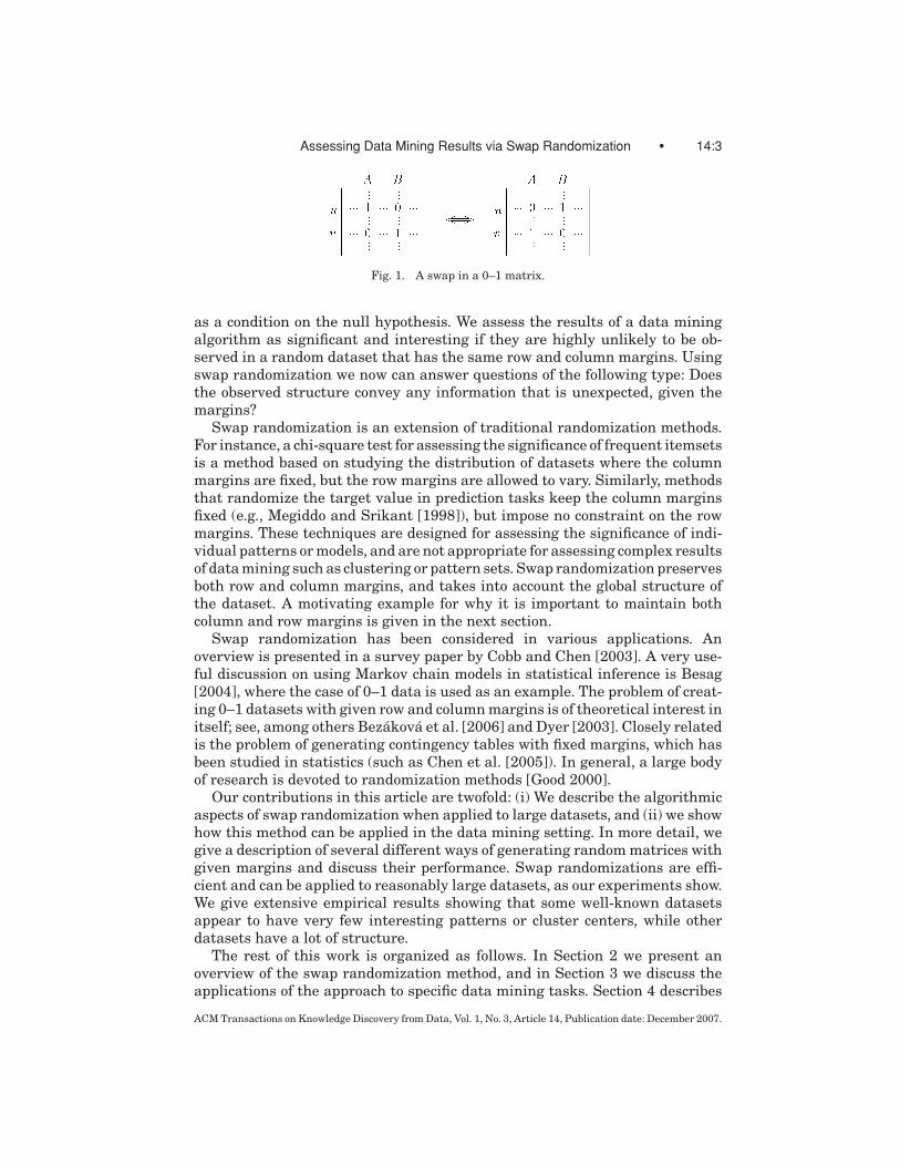
In statistics, the methods for significance testing are typically based eitheron analytical expressions or randomization tests. In this article we focus on thelatter approach. We propose the use of swap randomization [Cobb and Chen2003] for assessing data mining results on 0–1 datasets. The basic idea of swaprandomization is as follows. Given the dataset D, create random datasets withthe same row and column margins as D, run the data mining algorithm onthose, and see if the results are significantly different on the real data than onthe randomized datasets. If not, then we presume that the results are reallydue to the row and column margins, and not due to interesting relations in thedata. Generating datasets with the same margins as the original is performedby swaps, as shown in Figure 1: Take two rows u and v and two columns A andB of the data table with u(A) = v(B) = 1 and u(B) = v(A) = 0, and change therows so that u(B) = v(A) = 1 and u(A) = v(B) = 0. This operation maintainsthe row and column sums of the dataset, and all datasets with the same rowand column sums can be reached through a series of swaps [Ryser 1957; Cobband Chen 2003].
Swap randomization falls within the broad family of randomization testingmethods. Given a metric of interest (e.g., the number of frequent itemsets in thedata), randomization testing techniques produce multiple random datasets andtest the null hypothesis that the observed metric is likely to occur in the randomdata. If the metric of interest in the original data deviates significantly from themeasurements on the random datasets, then we can reject the null hypothesisand assess the result as significant. The key characteristic of the randomiza-tion techniques is in the way that the random datasets are generated. Ratherthan assuming that the underlying data follows a given distribution and sam-pling from this distribution, randomization techniques randomly shuffle thegiven data to produce a random dataset. Shuffling is meant to preserve someof the structural properties of the dataset, for example, in a 0–1 matrix we maywant to preserve the total number of 1’s in the dataset, or the number of 1’s ineach column. In the case of swap randomization, the generated samples pre-serve both the column and row margins. This constraint can also be thought of
ACM Transactions on Knowledge Discovery from Data, Vol. 1, No. 3, Article 14, Publication date: December 2007.
Assessing Data Mining Results via Swap Randomization • 14:3
Fig. 1. A swap in a 0–1 matrix.
as a condition on the null hypothesis. We assess the results of a data miningalgorithm as significant and interesting if they are highly unlikely to be ob-served in a random dataset that has the same row and column margins. Usingswap randomization we now can answer questions of the following type: Doesthe observed structure convey any information that is unexpected, given themargins?
Swap randomization is an extension of traditional randomization methods.For instance, a chi-square test for assessing the significance of frequent itemsetsis a method based on studying the distribution of datasets where the columnmargins are fixed, but the row margins are allowed to vary. Similarly, methodsthat randomize the target value in prediction tasks keep the column marginsfixed (e.g., Megiddo and Srikant [1998]), but impose no constraint on the rowmargins. These techniques are designed for assessing the significance of indi-vidual patterns or models, and are not appropriate for assessing complex resultsof data mining such as clustering or pattern sets. Swap randomization preservesboth row and column margins, and takes into account the global structure ofthe dataset. A motivating example for why it is important to maintain bothcolumn and row margins is given in the next section.
Swap randomization has been considered in various applications. Anoverview is presented in a survey paper by Cobb and Chen [2003]. A very use-ful discussion on using Markov chain models in statistical inference is Besag[2004], where the case of 0–1 data is used as an example. The problem of creat-ing 0–1 datasets with given row and column margins is of theoretical interest initself; see, among others Bezakova et al. [2006] and Dyer [2003]. Closely relatedis the problem of generating contingency tables with fixed margins, which hasbeen studied in statistics (such as Chen et al. [2005]). In general, a large bodyof research is devoted to randomization methods [Good 2000].
Our contributions in this article are twofold: (i) We describe the algorithmicaspects of swap randomization when applied to large datasets, and (ii) we showhow this method can be applied in the data mining setting. In more detail, wegive a description of several different ways of generating random matrices withgiven margins and discuss their performance. Swap randomizations are effi-cient and can be applied to reasonably large datasets, as our experiments show.We give extensive empirical results showing that some well-known datasetsappear to have very few interesting patterns or cluster centers, while otherdatasets have a lot of structure.
The rest of this work is organized as follows. In Section 2 we present anoverview of the swap randomization method, and in Section 3 we discuss theapplications of the approach to specific data mining tasks. Section 4 describes
ACM Transactions on Knowledge Discovery from Data, Vol. 1, No. 3, Article 14, Publication date: December 2007.

14:4 • A. Gionis et al.
how the random matrices with given margins are generated and provides re-sults on the performance of the algorithms. In Section 5 we describe the ex-perimental results. Section 6 discusses related work, and Section 7 gives someconcluding remarks.
2. OVERVIEW OF THE APPROACH
In this section we give an overview of the method. We explain the intuitionbehind it, describe the algorithmic challenges it poses, and show how it can beapplied to testing the significance of results obtained by different kinds of datamining algorithms.
2.1 The Randomization Approach
Let D denote a 0–1 matrix with m rows and n columns that represents ourdataset. We view the rows of the matrix as tuples in a database, and the columnsas items. The values 0–1 correspond to absence/presence of an item in the tuple.A large range of datasets can be represented in this format.
Assume that we are interested in assessing the result obtained by a partic-ular data mining algorithm A on input D. Let A(D) denote the result of thealgorithm. For simplicity, assume that it can be described by a single number.For instance, for frequent set mining algorithms, it can be the number of setswhose frequency exceeds a certain support threshold. Similarly, for a clusteringalgorithm, it can be the error of the clustering solution.
In our randomization approach we generate k datasets D1, . . . , Dk , such thateach Dt , t = 1, . . . , k, is an m×n 0–1 matrix that has the same row and columnsums as the original matrix D. Each dataset Dt is assumed to be a uniform andindependent sample from the space of all m × n 0–1 matrices with the givenmargins. The algorithm A is executed on each sampled dataset Dt , yieldingresults X t = A(Dt) for t = 1, . . . , k.
The significance of the result A(D) of the algorithm A on the dataset D istested by comparing it to the set X = {X 1, . . . , X k} of the results of A on thesampled datasets. If the output of the algorithm on the original data does notdeviate significantly from the values in X, then the result A(D) is not surprisingand its significance is small; otherwise, the result is considered to be statisticallysignificant.
The statistical significance of A(D) can be measured in a variety of ways.Assuming that the sampled datasets are independent and that k is large enoughso that X gives an approximation of the real distribution, then the empiricalp-value of X 0 = A(D) is
1
k + 1(min{|{t | X t < X 0}|, |{t | X t > X 0}|} + 1),
that is, the fraction of the random datasets in which we see a value more extremethan the value in the real data. The empirical p-value we compute considersboth the cases where the value X 0 is very small and very large compared to thevalues in X. Note that according to our definition the p-value takes values inthe interval [0, 0.5].
ACM Transactions on Knowledge Discovery from Data, Vol. 1, No. 3, Article 14, Publication date: December 2007.
Assessing Data Mining Results via Swap Randomization • 14:5
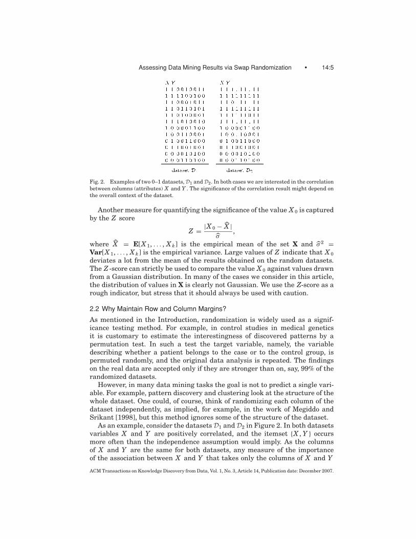
Fig. 2. Examples of two 0–1 datasets, D1 and D2. In both cases we are interested in the correlation
between columns (attributes) X and Y . The significance of the correlation result might depend on
the overall context of the dataset.
Another measure for quantifying the significance of the value X 0 is capturedby the Z score
Z = |X 0 − X |σ
,
where X = E[X 1, . . . , X k] is the empirical mean of the set X and σ 2 =Var[X 1, . . . , X k] is the empirical variance. Large values of Z indicate that X 0
deviates a lot from the mean of the results obtained on the random datasets.The Z -score can strictly be used to compare the value X 0 against values drawnfrom a Gaussian distribution. In many of the cases we consider in this article,the distribution of values in X is clearly not Gaussian. We use the Z-score as arough indicator, but stress that it should always be used with caution.
2.2 Why Maintain Row and Column Margins?
As mentioned in the Introduction, randomization is widely used as a signif-icance testing method. For example, in control studies in medical geneticsit is customary to estimate the interestingness of discovered patterns by apermutation test. In such a test the target variable, namely, the variabledescribing whether a patient belongs to the case or to the control group, ispermuted randomly, and the original data analysis is repeated. The findingson the real data are accepted only if they are stronger than on, say, 99% of therandomized datasets.
However, in many data mining tasks the goal is not to predict a single vari-able. For example, pattern discovery and clustering look at the structure of thewhole dataset. One could, of course, think of randomizing each column of thedataset independently, as implied, for example, in the work of Megiddo andSrikant [1998], but this method ignores some of the structure of the dataset.
As an example, consider the datasets D1 and D2 in Figure 2. In both datasetsvariables X and Y are positively correlated, and the itemset {X , Y } occursmore often than the independence assumption would imply. As the columnsof X and Y are the same for both datasets, any measure of the importanceof the association between X and Y that takes only the columns of X and Y
ACM Transactions on Knowledge Discovery from Data, Vol. 1, No. 3, Article 14, Publication date: December 2007.
14:6 • A. Gionis et al.
into account will give the same results for D1 and D2. However, in dataset D1,we see that X and Y cooccur in all types of rows, whereas in dataset D2 thecooccurrence of X and Y happens exclusively in very dense rows. Thus, inD2 thehigh frequency of the pair {X , Y } is not necessarily due to a correlation betweenX and Y , but rather to the fact that X and Y tend to occur on rows that have lotsof 1’s. For example, if X and Y are two items in a market-basket dataset, thentheir cooccurrence in D2 would be due to customers that buy almost all items.This finding is not as interesting, as it does not convey information specific toitems X and Y .
Consider the datasets E1 containing 10 copies of D1, and E2 containing 10copies ofD2. The columns for X and Y are the same in both datasets, and in bothcases the frequency of the pair is 60. When we generate 1000 random datasetswith the margins of E1, the maximum and average frequencies of {X , Y } were59 and 52.4, and the standard deviation was 2.5. All values were smaller than60, yielding an empirical p-value of 0.001. For E2 the corresponding numbersare 69, 63.2, and 2.0. In only 70 cases was the frequency 60 or less, giving anempirical p-value of 0.07. Thus, we can conclude that in E1 the pair {X , Y } isstrongly overrepresented, while in E2 it occurs less often than one would expect.This indicates that the context of the pair of variables has a strong effect on thesignificance of the frequency of a pair.
The previous example demonstrates the basic concept underlying swap ran-domization: It takes the bias of row and column counts into account by ran-domizing over datasets with the same row and column margins as the originaldataset. As a result, the notion of interestingness we consider is conditioned onthe knowledge of the marginal sums. We are interested in assessing informa-tion in the dataset that is not conveyed by the marginal sums of the data table.This is the structure that we define as being interesting.
As an additional example, consider a dataset whose margin counts satisfy apower-law distribution. The “heavy-tail” property of such a distribution impliesthat there exist rows and columns in the dataset with very high margin counts.It is possible that on such a dataset, a data mining algorithm discovers patternsthat are the direct consequence of the power-law distribution. For instance,columns with high margin counts will tend to form pairs that are much morefrequent than pairs of columns with very small margin counts. Alternatively,it is possible that a set of rows and columns with high margin counts is morelikely to form clearly distinguished biclusters. Using the framework of swaprandomization, one can assess whether a quantity of interest is immediatelyimplied by the power-law distribution on the margin counts, and thus whetherit is common to all datasets with the same margin distribution.
In general, a randomization procedure can be viewed as a random processwhich, given a dataset D, selects a dataset D1 from some class CD of datasetscontaining D. In swap randomization, the class CD is the set of all datasetshaving the same row and column margins as D. Varying the class CD defines adifferent randomization approach. In the independent permutation approach,the class CD contains all datasets with the same column sums as D. The rowsums are allowed to vary, so we expect the distribution to be fairly uniform. Asa consequence, the two methods differ significantly. A data mining result may
ACM Transactions on Knowledge Discovery from Data, Vol. 1, No. 3, Article 14, Publication date: December 2007.
Assessing Data Mining Results via Swap Randomization • 14:7
be deemed significant by the independent permutation method, but still beexplained purely by the row and column margins. We will see such an examplein the empirical section.
Maintaining row and column margins assumes that both row and columnsums are in some way interesting quantities. For example, consider ecologi-cal presence/absence data of species and locations, where rows to species andcolumns to locations. Then the column sums correspond to the commonnessof species, and row sums correspond to the species diversity of locations: Bothquantities are of fundamental interest in ecology, and hence maintaining themexactly makes sense. Similarly, consider a document dataset where rows cor-respond to documents and columns to words. Then row counts measure thenumber of different words in the document, and column sums indicate howwidely used is the word. In this case it is clear that the distributions of the rowand column sums are important properties of the dataset: In many cases theyexplain a lot of the observed structure of the data. Generating random datasetsthat maintain these sums makes it possible to see whether some structure isunexpected, given the margins.
There are other techniques of randomization. For example, instead of requir-ing that the row and column margins are maintained exactly, we could requirethat they are maintained approximately. One possible condition is to requirethat the L1-distance between the row margins of D and D1 is bounded. Anotherrandomization procedure could be obtained by requiring that the distributionof row and column margins is approximately the same in D and D1.
2.3 Limitations of the Approach
Summarizing the previous section, we believe that comparison of datasets withthe same margins provides a good method for assessing the significance ofthe discovered patterns. However, what constitutes an interesting pattern isnot well defined and often can be very subjective. Therefore, we do not claimthat swap randomization is a panacea for assessing all potential notions ofinterestingness. In fact, through the framework of swap randomization theconcept of interestingness takes a very precise definition: Interesting patternsare those that are not likely to appear in datasets with the same margins asthe input dataset. Having a precise definition of interestingness is certainly adesirable property, but it is possible that there are many other intuitive conceptsof interestingness that are not captured by this definition.
Consider a binary dataset in which half of the rows contain only 1’s and theother half only 0’s. This particular dataset is the unique dataset with those exactmargins, and, according to the swap randomization framework, no pattern willbe considered interesting even though the dataset has very interesting struc-ture. The point here is that we must remember that swap randomization doesnothing more than compare datasets with the same margins. In this particularexample, the technique reports that there is no interesting structure, given themargins of the dataset. In fact, one can argue that all the interesting structureof the dataset is expected given the margins, since this is the only dataset withthese margins.
ACM Transactions on Knowledge Discovery from Data, Vol. 1, No. 3, Article 14, Publication date: December 2007.
14:8 • A. Gionis et al.
Another limitation of the swap randomization framework, as presented inthis article, is that it is applied only to data with 0–1 values, which denoteabsence or presence of an attribute value. Many datasets can be modeled as0–1 matrices; examples include market-basket data, word occurrences in docu-ments and access logs, data from scientific applications such as biology, ecology,paleontology, and more. However, many other datasets require more generalrepresentations. Two important cases widely studied in the literature are nu-merical data and categorical data.
For numerical data one possible extension is generate datasets in which thesums of the entries of all rows and all columns are fixed. This is the problemof sampling from the space of contingency tables and it has been studied ex-tensively in the statistics literature [Chen et al. 2005; Cobb and Chen 2003;Diaconis and Gangolli 1995; Snijders 1991]. One basic technique is to sampleby performing a random walk on the Diaconis chain [Diaconis and Saloff-Coste1995], which is a generalization of the basic swap move shown in Figure 1. Amove on the Diaconis chain consists of randomly selecting two rows i and jand two columns k and l , and adding the values 1, −1, −1, and 1 at the entries(i, k), (i, l ), ( j , k), and ( j , l ) (respectively) of the current matrix, as long as noentry becomes negative.
In order to apply the framework to numerical data, in addition to the tech-nical modifications, it must be verified that it is meaningful to maintain rowand column sums. For instance, it arguably makes sense to maintain row andcolumn sums in a dataset in which the presence or absence information ofwords in documents is replaced with counts. On the other hand, it is clearlynot meaningful to maintain row and column sums in a dataset with the nu-merical attributes age, income, and num of children. Similarly, the swap ran-domization framework does not seem to be applicable to data with categoricalattributes, even if these attributes have a binary domain. Consider a datasetwith attributes gender, education, and employment status. It is not clear howto perform the basic swap moves, or what are the margins we wish to maintain.
2.4 Generating Matrices with Given Margins
Generating random 0–1 datasets with given row and column sums is a technicalchallenge. This problem has been studied extensively in statistics [Chen et al.2005; Cobb and Chen 2003], theoretical computer science [Bezakova et al. 2006;Dyer 2003], and in various application areas [Kashtan et al. 2004; Milo et al.2002].
In this article we use a Markov chain approach to the problem of sampling.Starting from the original dataset, we make a small random local move whichinterchanges a pair of 1’s with a pair of 0’s and does not change the row andcolumn sums, thus producing a new dataset with the same margins. Such alocal move is called a swap, and a sequence of swaps is performed until the datais sufficiently mixed to provide a random sample. In the swap randomizationframework we want to compare the input dataset with random datasets thathave the same margins. Since we have no reason to assume that any of thesedatasets is more likely than the others, we would like to sample uniformly from
ACM Transactions on Knowledge Discovery from Data, Vol. 1, No. 3, Article 14, Publication date: December 2007.
Assessing Data Mining Results via Swap Randomization • 14:9
the set of all possible datasets. Uniform sampling avoids introducing any sam-pling bias to the significance test. In the language of Markov chains we want toensure that the stationary distribution of the chain is the uniform distribution.
The state space of the Markov chain consists of all datasets with the givenmargins. There is a transition between two datasets if there is a swap thattransforms one to the other. The Markov chain is reversible, that is, a swapcan be undone by a single (reverse) swap. However, the chain is not regular, assome datasets (states) have more neighbors than others. This implies that thestationary distribution of the chain is not the uniform distribution. Therefore, astraightforward application of swapping does not guarantee uniform sampling.
The problem of nonuniformity can be fixed in at least two ways: (i) by us-ing the Metropolis-Hastings algorithm [Hastings 1970; Metropolis et al. 1953],which is a well-studied method for converting one Markov chain with station-ary distribution π to another with stationary distribution π ′; and (ii) by addingmultiple self-loops in order to guarantee that all states have the same degree.
For applying the Metropolis-Hastings algorithm, one needs to compute thedegree of any given state of the chain, that is, the number of all valid swaps fora given 0–1 matrix. We give a simple formula for computing the degree at eachstate, and we show how to maintain this quantity incrementally. The complexityof incremental maintenance of the state degree is O(min{m, n}) for an m × nmatrix, making the algorithm somehow inefficient. On the other hand, addingself-loops does not require computing any additional expensive information; sowhile more steps are needed for convergence, the time complexity of each stepis, in expectation, constant, making it a very efficient algorithm in practice.
3. USING THE FRAMEWORK
In this section we describe how the swap randomization framework can beapplied to different data mining tasks, such as finding frequent sets and corre-lations, clustering, and spectral analysis. Our methodology allows us to inves-tigate the significance of the patterns that exist in a given dataset, at differentlevels of granularity.
First, we are able to characterize the significance of global aspects of thedataset. If the number of frequent sets, or the number of highly correlatedpairs contained in the dataset, is not significant with respect to that found in arandomly rearranged dataset, then we can conclude that the dataset does notcontain any interesting global structure of frequent sets, or of highly significantcorrelations.
Additionally, we can also look at individual itemsets. In this case we areinterested in identifying itemsets whose frequency is smaller or larger in thesampled datasets when compared with the original dataset. If the frequencyof an itemset drops in the sampled dataset, it is implied that the frequencycannot be explained by the margins of the dataset. If the frequency increases,a possible explanation is that the items in the itemset are anticorrelated in theoriginal dataset.
The aforesaid observations also apply when mining simple association rules.Recall that the accuracy (confidence) of a rule (X ⇒ B) is defined as f (X B)
f (X ),
ACM Transactions on Knowledge Discovery from Data, Vol. 1, No. 3, Article 14, Publication date: December 2007.
14:10 • A. Gionis et al.
where f (X B) and f (X ) are the frequencies of X ∪ {B} and {X }, respectively.Assume now that X is a singleton set. Since f (X ) remains fixed, the confidenceof the rule is proportional to the frequency f (X B). Therefore, the significanceof the rule (X ⇒ B) is determined by the significance of the pair {X , B}. In thegeneral case that the set {X } consists of more than one item, our observationthat the confidence of (X ⇒ B) depends only on the frequencies of f (X B) andf (X ) still holds. Thus, we can assess the significance of the rule (X ⇒ B) bykeeping track of the frequencies of the sets X ∪ {B} and {X } on the sampledatasets that we generate during the swap randomization process. Overall, forthe framework of swap randomization, the case of association rules is subsumedby the analysis of frequent itemsets.
Swap randomization can be applied to testing the significance of clusteringresults. Given a clustering algorithm like k-means and a target number ofclusters k, we compare the clustering error in the original dataset with that inthe sampled datasets. If the difference is large, then we can deduce that thedataset has meaningful cluster structure. This simple approach turns out toyield very clear results on synthetic datasets with known cluster structure, aswe will see in Section 5.
To obtain some intuition of how clustering structure is related to row andcolumn margins, consider the very simple and rather contrived dataset D whichhas n rows, n columns, and k “pure” clusters. Here, by pure clusters we meanthat the data matrix is block diagonal with k blocks of 1’s, each of size n
k × nk ,
and the rest of the matrix entries are 0’s. Therefore all the row and columnmargins are n
k , and there is a perfect clustering into k clusters with error 0. Onthe other hand, it is true that a random dataset with the same margins as D hasno clustered structure; each entry of the data matrix of such a random datasetappears to be almost random with probability 1
k , and the error of clustering into
k clusters is roughly O( 1k (1 − 1
k )n2).A different notion of global structure is captured in the singular values and
vectors of the data matrix. Singular vectors capture linear trends in the dataset.The corresponding singular values capture the strength of the linear trend, thatis, the tendency of rows or columns to align with corresponding singular vectors.The strongest linear trends can be used to construct a low-dimensional approx-imation of the dataset with provable approximation error. In randomly gener-ated data, the strongest linear trends should be determined by the marginalsof the dataset. This is usually the first singular value. The remaining datasethas no structure; thus we expect the remaining singular values to be small.If the original data contains some linear structure, then the top singular val-ues (especially the nonprincipal ones) should be higher than those of randomdatasets with the same margins.
4. SAMPLING DATASETS WITH GIVEN ROW AND COLUMN MARGINS
4.1 Basics
We now describe the process of sampling a matrix from the space of all m × n0–1 matrices with given margins.
ACM Transactions on Knowledge Discovery from Data, Vol. 1, No. 3, Article 14, Publication date: December 2007.
Assessing Data Mining Results via Swap Randomization • 14:11
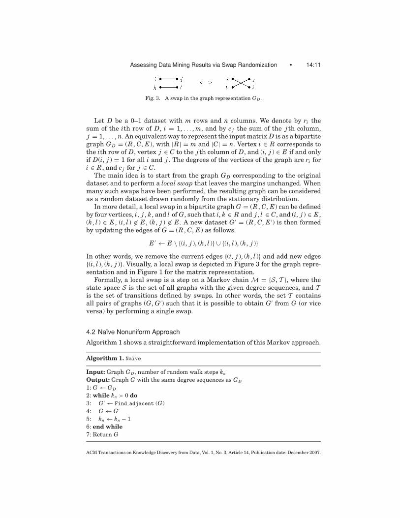
Fig. 3. A swap in the graph representation GD .
Let D be a 0–1 dataset with m rows and n columns. We denote by ri thesum of the ith row of D, i = 1, . . . , m, and by c j the sum of the j th column,j = 1, . . . , n. An equivalent way to represent the input matrix D is as a bipartitegraph GD = (R, C, E), with |R| = m and |C| = n. Vertex i ∈ R corresponds tothe ith row of D, vertex j ∈ C to the j th column of D, and (i, j ) ∈ E if and onlyif D(i, j ) = 1 for all i and j . The degrees of the vertices of the graph are ri fori ∈ R, and c j for j ∈ C.
The main idea is to start from the graph GD corresponding to the originaldataset and to perform a local swap that leaves the margins unchanged. Whenmany such swaps have been performed, the resulting graph can be consideredas a random dataset drawn randomly from the stationary distribution.
In more detail, a local swap in a bipartite graph G = (R, C, E) can be definedby four vertices, i, j , k, and l of G, such that i, k ∈ R and j , l ∈ C, and (i, j ) ∈ E,(k, l ) ∈ E, (i, l ) �∈ E, (k, j ) �∈ E. A new dataset G ′ = (R, C, E ′) is then formedby updating the edges of G = (R, C, E) as follows.
E ′ ← E \ {(i, j ), (k, l )} ∪ {(i, l ), (k, j )}In other words, we remove the current edges {(i, j ), (k, l )} and add new edges{(i, l ), (k, j )}. Visually, a local swap is depicted in Figure 3 for the graph repre-sentation and in Figure 1 for the matrix representation.
Formally, a local swap is a step on a Markov chain M = {S, T }, where thestate space S is the set of all graphs with the given degree sequences, and Tis the set of transitions defined by swaps. In other words, the set T containsall pairs of graphs (G, G ′) such that it is possible to obtain G ′ from G (or viceversa) by performing a single swap.
4.2 Naıve Nonuniform Approach
Algorithm 1 shows a straightforward implementation of this Markov approach.
Algorithm 1. Naıve
Input: Graph GD, number of random walk steps kn
Output: Graph G with the same degree sequences as GD
1: G ← GD
2: while kn > 0 do3: G ′ ← Find adjacent (G)
4: G ← G ′
5: kn ← kn − 1
6: end while7: Return G
ACM Transactions on Knowledge Discovery from Data, Vol. 1, No. 3, Article 14, Publication date: December 2007.
14:12 • A. Gionis et al.
Finding the next transition (G, G ′) ∈ T from graph G, that is, executing line3 of algorithm Naıve, is not a completely straightforward task. The simplestway is to pick a pair of edges in G, reject if the edges are not swappable, andrepeat until a pair of swappable edges is found. This is shown in Algorithm 2.Alternatively, one could store all swappable pairs in a structure and selectone uniformly at random. The selection process becomes faster, but there isadditional cost of updating the data structure at each step.
Algorithm 2. Find adjacent
Input: Graph GOutput: Graph G ′ that differs from G in exactly one swap (i.e., (G, G ′) ∈ T )
repeatSelect edges (i, j ), (k, l ) ∈ E(G) uniformly at random
until (i, l ) �∈ E(G) and (k, j ) �∈ E(G)
E(G ′) ← E(G) \ {(i, j ), (k, l )} ∪ {(i, l ), (k, j )}
Given graph G, the algorithm Find adjacent generates a graph G ′ uniformlyat random among all graphs G ′ such that (G, G ′) ∈ T . The reason is that thereexists an one-to-one correspondence between the set of such graphs G ′ and theset of swappable pairs of edges: Each graph G ′ is mapped to exactly one uniqueswappable pair, and for each swappable pair there exists a unique graph G ′.Algorithm Find adjacent clearly samples uniformly at random from the set ofswappable pairs: Each swappable pair is sampled with probability proportionalto 2/|E|2.
Now, in order for the Markov chain to sample graphs uniformly at randomfrom the set S, the following conditions have to hold:
(1) The state space S is connected under the transitions of M.
(2) The Markov chain M has a uniform stationary distribution.
(3) Starting from GD, a sufficiently large number of local swaps should beperformed so that the chain mixes. We would like to know how many suchswaps should be performed, namely, the mixing time of the chain.
Connectedness. The Markov chain is connected. One can move from anystate of the chain to any other state using swaps [Ryser 1957; Cobb and Chen2003].
Uniformity. First notice that the Markov chain M is reversible. Now, for eachgraph (state) G ∈ S, we define d (G), namely the degree of the Markov chainM at G, to be the number of different graphs (states) G ′ such that (G, G ′) ∈T . From the theory of Markov chains, it is well known that the stationarydistribution of a reversible chain is proportional to the degree at each statein the underlying transition graph. Therefore, in order to obtain a uniformdistribution, all states of the Markov chain must have the same degree. A simpleconstruction shows that this is not true in general for the Markov chain M.Therefore, the Naıve algorithm (Algorithm 1) does not converge to the uniformdistribution.
ACM Transactions on Knowledge Discovery from Data, Vol. 1, No. 3, Article 14, Publication date: December 2007.
Assessing Data Mining Results via Swap Randomization • 14:13
Mixing time. The mixing time of the Markov chain we defined previouslyhas been the object of theoretical study [Cobb and Chen 2003], but without anyconclusive results. It is estimated that running the chain for a number of stepsin order of the number of 1’s in the matrix is sufficient for convergence. Wedo not deal with theoretical aspects of convergence, but study it empirically inthe experimental section. See Besag [2004] for a discussion on convergence andp-values.
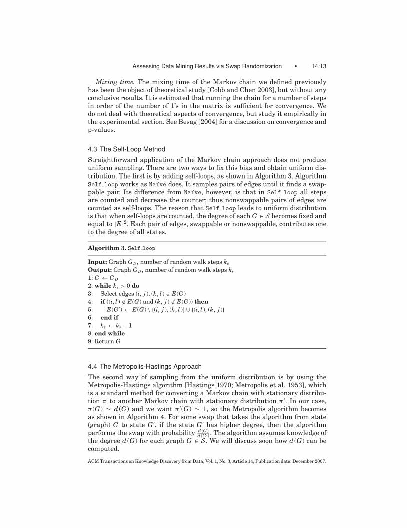
4.3 The Self-Loop Method
Straightforward application of the Markov chain approach does not produceuniform sampling. There are two ways to fix this bias and obtain uniform dis-tribution. The first is by adding self-loops, as shown in Algorithm 3. AlgorithmSelf loop works as Naıve does. It samples pairs of edges until it finds a swap-pable pair. Its difference from Naıve, however, is that in Self loop all stepsare counted and decrease the counter; thus nonswappable pairs of edges arecounted as self-loops. The reason that Self loop leads to uniform distributionis that when self-loops are counted, the degree of each G ∈ S becomes fixed andequal to |E|2. Each pair of edges, swappable or nonswappable, contributes oneto the degree of all states.
Algorithm 3. Self loop
Input: Graph GD, number of random walk steps ks
Output: Graph GD, number of random walk steps ks
1: G ← GD
2: while ks > 0 do3: Select edges (i, j ), (k, l ) ∈ E(G)
4: if ((i, l ) �∈ E(G) and (k, j ) �∈ E(G)) then5: E(G ′) ← E(G) \ {(i, j ), (k, l )} ∪ {(i, l ), (k, j )}6: end if7: ks ← ks − 1
8: end while9: Return G
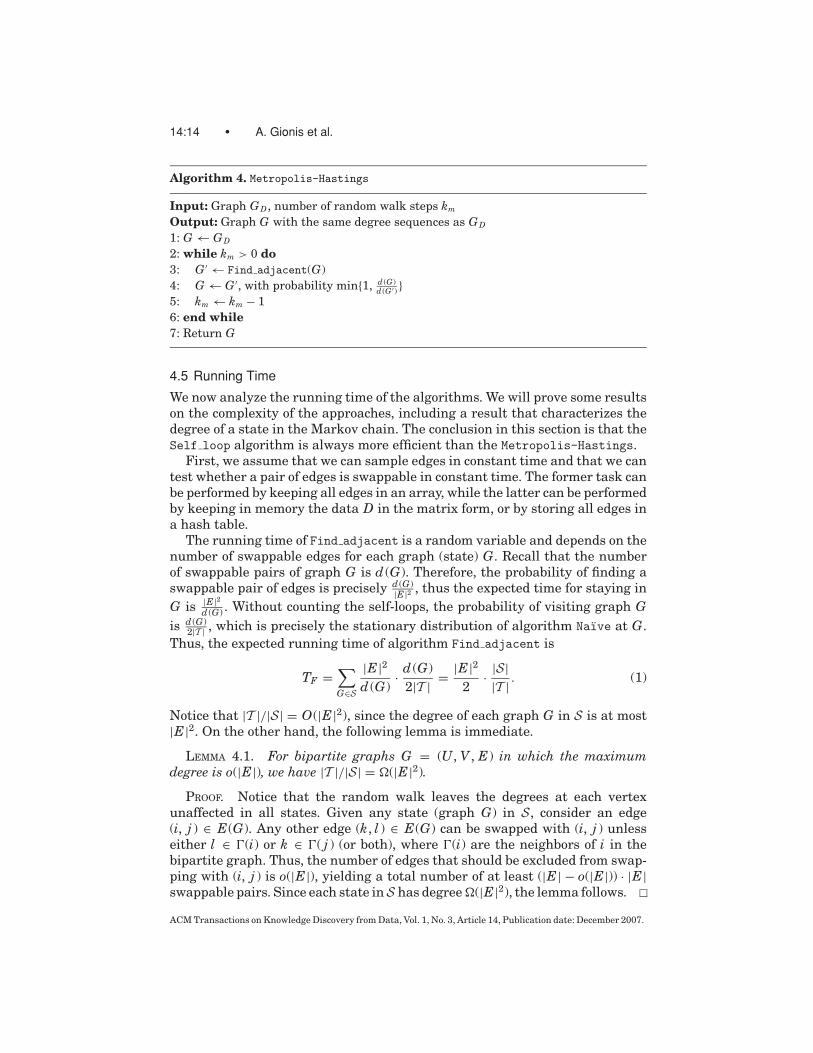
4.4 The Metropolis-Hastings Approach
The second way of sampling from the uniform distribution is by using theMetropolis-Hastings algorithm [Hastings 1970; Metropolis et al. 1953], whichis a standard method for converting a Markov chain with stationary distribu-tion π to another Markov chain with stationary distribution π ′. In our case,π (G) ∼ d (G) and we want π ′(G) ∼ 1, so the Metropolis algorithm becomesas shown in Algorithm 4. For some swap that takes the algorithm from state(graph) G to state G ′, if the state G ′ has higher degree, then the algorithmperforms the swap with probability d (G)
d (G ′) . The algorithm assumes knowledge ofthe degree d (G) for each graph G ∈ S. We will discuss soon how d (G) can becomputed.
ACM Transactions on Knowledge Discovery from Data, Vol. 1, No. 3, Article 14, Publication date: December 2007.
14:14 • A. Gionis et al.
Algorithm 4. Metropolis-Hastings
Input: Graph GD, number of random walk steps km
Output: Graph G with the same degree sequences as GD
1: G ← GD
2: while km > 0 do3: G ′ ← Find adjacent(G)
4: G ← G ′, with probability min{1, d (G)d (G′) }
5: km ← km − 1
6: end while7: Return G
4.5 Running Time
We now analyze the running time of the algorithms. We will prove some resultson the complexity of the approaches, including a result that characterizes thedegree of a state in the Markov chain. The conclusion in this section is that theSelf loop algorithm is always more efficient than the Metropolis-Hastings.
First, we assume that we can sample edges in constant time and that we cantest whether a pair of edges is swappable in constant time. The former task canbe performed by keeping all edges in an array, while the latter can be performedby keeping in memory the data D in the matrix form, or by storing all edges ina hash table.
The running time of Find adjacent is a random variable and depends on thenumber of swappable edges for each graph (state) G. Recall that the numberof swappable pairs of graph G is d (G). Therefore, the probability of finding aswappable pair of edges is precisely d (G)
|E|2 , thus the expected time for staying in
G is |E|2d (G)
. Without counting the self-loops, the probability of visiting graph Gis d (G)
2|T | , which is precisely the stationary distribution of algorithm Naıve at G.
Thus, the expected running time of algorithm Find adjacent is
TF =∑G∈S
|E|2d (G)
· d (G)
2|T | = |E|22
· |S||T | . (1)
Notice that |T |/|S| = O(|E|2), since the degree of each graph G in S is at most|E|2. On the other hand, the following lemma is immediate.
LEMMA 4.1. For bipartite graphs G = (U, V , E) in which the maximumdegree is o(|E|), we have |T |/|S| = �(|E|2).
PROOF. Notice that the random walk leaves the degrees at each vertexunaffected in all states. Given any state (graph G) in S, consider an edge(i, j ) ∈ E(G). Any other edge (k, l ) ∈ E(G) can be swapped with (i, j ) unlesseither l ∈ �(i) or k ∈ �( j ) (or both), where �(i) are the neighbors of i in thebipartite graph. Thus, the number of edges that should be excluded from swap-ping with (i, j ) is o(|E|), yielding a total number of at least (|E| − o(|E|)) · |E|swappable pairs. Since each state inS has degree �(|E|2), the lemma follows.
ACM Transactions on Knowledge Discovery from Data, Vol. 1, No. 3, Article 14, Publication date: December 2007.
Assessing Data Mining Results via Swap Randomization • 14:15
COROLLARY 4.2. For bipartite graphs G = (U, V , E) whose degree distribu-tion follows a power law with α > 2 we have |T |/|S| = �(|E|2).
PROOF. For simplicity assume that |U | = |V | = n. For power laws withexponent α > 2 we have |E| = O(n) in expectation and the maximum degree is
n1
α−1 = o(n) (e.g., see Newman [2003]). Thus, the conditions of Lemma 4.1 aresatisfied.
The preceding results imply that for some important classes of datasets (suchas graphs with bounded degrees or degrees that follow a power-law distribution)the expected time TF of the Find adjacent algorithm is constant. Thus, for thoseclasses of data, the running time of algorithm Naıve is TN = TF · kn = O(kn).Similarly, for the Self loop algorithm the overall running time is TS = O(ks).Furthermore, the expected time spent in each state for performing self-loops(before moving out to a new state) is constant.
We now turn to the running time of Metropolis-Hastings. This runningtime can be written as TM = T 0
D + km(TF + TD), where TF is the running timeof Find adjacent, TD is the time needed to compute d (G ′) given that d (G) isalready computed, and T 0
D is the time needed to compute d (G) for the first time.Next we explain how to compute d (G) and how to update the computation ford (G ′). The time needed for the update is linear with respect to min{m, n}.
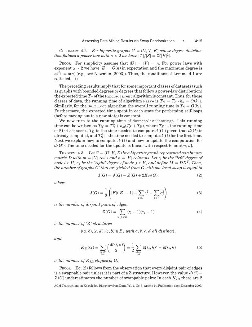
THEOREM 4.3. Let G = (U, V , E) be a bipartite graph represented as a binarymatrix D with m = |U | rows and n = |V | columns. Let ri be the “left” degree ofnode i ∈ U, c j be the “right” degree of node j ∈ V , and define M = DDT . Then,the number of graphs G ′ that are yielded from G with one local swap is equal to
d (G) = J (G) − Z (G) + 2K22(G), (2)
where
J (G) = 1
2
(|E|(|E| + 1) −
∑i∈U
r2i −
∑j∈V
c2j
)(3)
is the number of disjoint pairs of edges,
Z (G) =∑
(i, j )∈E
(ri − 1)(c j − 1) (4)
is the number of “Z” structures
{(a, b), (c, d ), (c, b) ∈ E, with a, b, c, d all distinct},and
K22(G) =∑i,k∈Ui �=k
(M (i, k)
2
)= 1
2
∑i,k∈Ui �=k
M (i, k)2 − M (i, k) (5)
is the number of K2,2 cliques of G.
PROOF. Eq. (2) follows from the observation that every disjoint pair of edgesis a swappable pair unless it is part of a Z structure. However, the value J (G)−Z (G) underestimates the number of swappable pairs: In each K2,2 there are 2
ACM Transactions on Knowledge Discovery from Data, Vol. 1, No. 3, Article 14, Publication date: December 2007.
14:16 • A. Gionis et al.
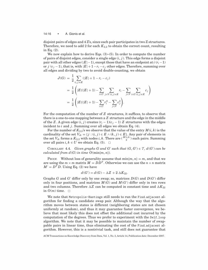
disjoint pairs of edges and 4 Z’s, since each pair participates in two Z structures.Therefore, we need to add 2 for each K2,2 to obtain the correct count, resultingin Eq. (2).
We now explain how to derive Eqs. (3)–(5). In order to compute the numberof pairs of disjoint edges, consider a single edge (i, j ). This edge forms a disjointpair with all other edges (|E|−1), except those that have an endpoint at i (ri −1)or j (c j −1), that is, with |E|+1−ri − c j other edges. Therefore, summing overall edges and dividing by two to avoid double-counting, we obtain
J (G) = 1
2
∑(i, j )∈E
(|E| + 1 − ri − c j )
= 1
2
(|E|(|E| + 1) −
∑i∈U
∑j∈V :(i, j )∈E
ri −∑j∈V
∑i∈U :(i, j )∈E
c j
)
= 1
2
(|E|(|E| + 1) −
∑i∈U
r2i −
∑j∈V
c2j
).
For the computation of the number of Z structures, it suffices, to observe thatthere is a one-to-one mapping between a Z structure and the edge in the middleof the Z . A given edge (i, j ) creates (ri − 1)(c j − 1) Z structures with the edgesincident to i and j . Summing over all edges we obtain Eq. (4).
For the number of K2,2’s we observe that the value of the entry M (i, k) is thecardinality of the set Vik = { j : (i, j ) ∈ E ∧ (k, j ) ∈ E}. Any pair of elements inthe set Vik forms a K2,2 with nodes i, k. There are ( M (i,k)
2) such pairs. Summing
over all pairs i, k ∈ U we obtain Eq. (5).
COROLLARY 4.4. Given graphs G and G ′ such that (G, G ′) ∈ T , d (G ′) can becalculated from d (G) in time O(min{m, n}).
PROOF. Without loss of generality assume that min{m, n} = m, and that weare using the m × m matrix M = DDT . Otherwise we can use the n × n matrixM ′ = DT D. Using Eq. (2) we have
d (G ′) = d (G) − �Z + 2 �K22.
Graphs G and G ′ differ only by one swap; so, matrices D(G) and D(G ′) differonly in four positions, and matrices M (G) and M (G ′) differ only in two rowsand two columns. Therefore �Z can be computed in constant time and �K22
in O(m) time.
We note that Metropolis-Hastings still needs to run the Find adjacent al-gorithm for finding a candidate swap pair. Although the way that the algo-rithm moves between states is different (neighboring states are not chosenuniformly at random), and thus it may guarantee faster convergence, we be-lieve that most likely this does not offset the additional cost incurred by thecomputation of the degrees. Thus we prefer to experiment with the Self loopalgorithm. We note that it may be possible to maintain the number of swap-pable pairs in linear time, thus eliminating the cost of the Find adjacent al-gorithm. However, this is a nontrivial task, and still does not guarantee that
ACM Transactions on Knowledge Discovery from Data, Vol. 1, No. 3, Article 14, Publication date: December 2007.
Assessing Data Mining Results via Swap Randomization • 14:17
Table I. The Datasets
Dataset # of rows # of cols # of 1’s dens. (%)
ABSTRACTS 128820 25335 10449902 0.32
ABSTRACTS′ 128803 5918 7150992 0.94
COURSES 2405 5021 65152 0.54
KOSARAK 990002 41270 8019015 0.02
PALEO 124 139 1978 11.48
RETAIL 88162 16470 908576 0.06
the Metropolis-Hastings algorithm would be faster. Recall also that in manycases, the cost of Find adjacent is constant in expectation.
5. EMPIRICAL RESULTS
We perform experiments with many of the well-known datasets used in the datamining community. A description of the datasets we are using is as follows: AB-STRACTS contains document-word information on a collection of project abstractssubmitted for funding by NSF. ABSTRACTS
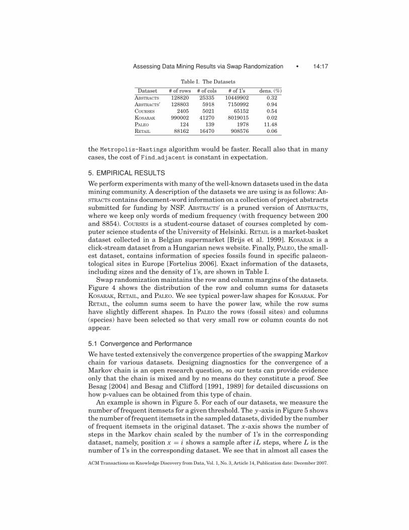
′ is a pruned version of ABSTRACTS,where we keep only words of medium frequency (with frequency between 200and 8854). COURSES is a student-course dataset of courses completed by com-puter science students of the University of Helsinki. RETAIL is a market-basketdataset collected in a Belgian supermarket [Brijs et al. 1999]. KOSARAK is aclick-stream dataset from a Hungarian news website. Finally, PALEO, the small-est dataset, contains information of species fossils found in specific palaeon-tological sites in Europe [Fortelius 2006]. Exact information of the datasets,including sizes and the density of 1’s, are shown in Table I.
Swap randomization maintains the row and column margins of the datasets.Figure 4 shows the distribution of the row and column sums for datasetsKOSARAK, RETAIL, and PALEO. We see typical power-law shapes for KOSARAK. ForRETAIL, the column sums seem to have the power law, while the row sumshave slightly different shapes. In PALEO the rows (fossil sites) and columns(species) have been selected so that very small row or column counts do notappear.
5.1 Convergence and Performance
We have tested extensively the convergence properties of the swapping Markovchain for various datasets. Designing diagnostics for the convergence of aMarkov chain is an open research question, so our tests can provide evidenceonly that the chain is mixed and by no means do they constitute a proof. SeeBesag [2004] and Besag and Clifford [1991, 1989] for detailed discussions onhow p-values can be obtained from this type of chain.
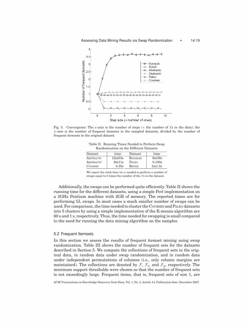
An example is shown in Figure 5. For each of our datasets, we measure thenumber of frequent itemsets for a given threshold. The y-axis in Figure 5 showsthe number of frequent itemsets in the sampled datasets, divided by the numberof frequent itemsets in the original dataset. The x-axis shows the number ofsteps in the Markov chain scaled by the number of 1’s in the correspondingdataset, namely, position x = i shows a sample after iL steps, where L is thenumber of 1’s in the corresponding dataset. We see that in almost all cases the
ACM Transactions on Knowledge Discovery from Data, Vol. 1, No. 3, Article 14, Publication date: December 2007.

14:18 • A. Gionis et al.
Fig. 4. Distribution of row and column sums in KOSARAK, RETAIL, and PALEO datasets. Log-log scale.
chain mixes quite rapidly: Already after L steps (4L in the case of KOSARAK) thenumber of frequent sets has stabilized.
Similar convergence evidence was obtained for all our measures: frequenciesof specific itemsets, number of correlations above a certain threshold, clusteringerrors, etc. In all of the experiments presented in the following sections we haverun the chain with a very large number of steps in order to ensure convergence.
ACM Transactions on Knowledge Discovery from Data, Vol. 1, No. 3, Article 14, Publication date: December 2007.
Assessing Data Mining Results via Swap Randomization • 14:19
Fig. 5. Convergence: The x-axis is the number of steps (× the number of 1’s in the data); the
y-axis is the number of frequent itemsets in the sampled datasets, divided by the number of
frequent itemsets in the original dataset.
Table II. Running Times Needed to Perform Swap
Randomization on the Different Datasets
Dataset time
ABSTRACTS 12m53s
ABSTRACTS′ 9m11s
COURSES 3.35s
Dataset time
KOSARAK 8m38s
PALEO 0.100s
RETAIL 1m1.5s
We report the clock time (in s) needed to perform a number of
swaps equal to 5 times the number of the 1’s in the dataset.
Additionally, the swaps can be performed quite efficiently. Table II shows therunning time for the different datasets, using a simple Perl implementation ona 3GHz Pentium machine with 2GB of memory. The reported times are forperforming 5L swaps. In most cases a much smaller number of swaps can beused. For comparison, the time needed to cluster the COURSES and PALEO datasetsinto 5 clusters by using a simple implementation of the K-means algorithm are60 s and 1 s, respectively. Thus, the time needed for swapping is small comparedto the need for running the data mining algorithm on the samples.
5.2 Frequent Itemsets
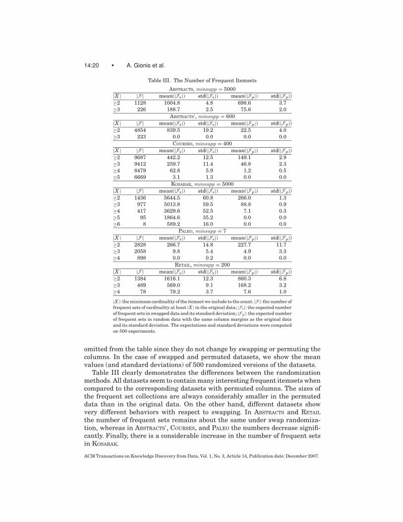
In this section we assess the results of frequent itemset mining using swaprandomization. Table III shows the number of frequent sets for the datasetsdescribed in Section 5. We compute the collections of frequent sets in the orig-inal data, in random data under swap randomization, and in random dataunder independent permutations of columns (i.e., only column margins aremaintained). The collections are denoted by F , Fs, and Fp, respectively. Theminimum support thresholds were chosen so that the number of frequent setsis not exceedingly large. Frequent items, that is, frequent sets of size 1, are
ACM Transactions on Knowledge Discovery from Data, Vol. 1, No. 3, Article 14, Publication date: December 2007.
14:20 • A. Gionis et al.
Table III. The Number of Frequent Itemsets
ABSTRACTS, minsupp = 5000
|X | |F | mean(|Fs|) std(|Fs|) mean(|Fp|) std(|Fp|)≥2 1128 1004.8 4.8 698.6 3.7
≥3 226 188.7 2.5 75.6 2.0
ABSTRACTS′, minsupp = 600
|X | |F | mean(|Fs|) std(|Fs|) mean(|Fp|) std(|Fp|)≥2 4854 839.5 19.2 22.5 4.0
≥3 223 0.0 0.0 0.0 0.0
COURSES, minsupp = 400
|X | |F | mean(|Fs|) std(|Fs|) mean(|Fp|) std(|Fp|)≥2 9687 442.2 12.5 149.1 2.9
≥3 9412 259.7 11.4 46.8 2.3
≥4 8479 62.8 5.9 1.2 0.5
≥5 6669 3.1 1.3 0.0 0.0
KOSARAK, minsupp = 5000
|X | |F | mean(|Fs|) std(|Fs|) mean(|Fp|) std(|Fp|)≥2 1436 5644.5 60.8 266.0 1.3
≥3 977 5013.8 59.5 88.8 0.9
≥4 417 3629.6 52.5 7.1 0.3
≥5 95 1864.6 35.2 0.0 0.0
≥6 8 589.2 16.0 0.0 0.0
PALEO, minsupp = 7
|X | |F | mean(|Fs|) std(|Fs|) mean(|Fp|) std(|Fp|)≥2 2828 266.7 14.8 227.7 11.7
≥3 2058 9.8 5.4 4.9 3.3
≥4 898 0.0 0.2 0.0 0.0
RETAIL, minsupp = 200
|X | |F | mean(|Fs|) std(|Fs|) mean(|Fp|) std(|Fp|)≥2 1384 1616.1 12.3 860.3 6.8
≥3 489 569.0 9.1 168.2 3.2
≥4 78 79.2 3.7 7.6 1.0
|X |: the minimum cardinality of the itemset we include to the count. |F |: the number of
frequent sets of cardinality at least |X | in the original data; |Fs|: the expected number
of frequent sets in swapped data and its standard deviation; |Fp|: the expected number
of frequent sets in random data with the same column margins as the original data
and its standard deviation. The expectations and standard deviations were computed
on 500 experiments.
omitted from the table since they do not change by swapping or permuting thecolumns. In the case of swapped and permuted datasets, we show the meanvalues (and standard deviations) of 500 randomized versions of the datasets.
Table III clearly demonstrates the differences between the randomizationmethods. All datasets seem to contain many interesting frequent itemsets whencompared to the corresponding datasets with permuted columns. The sizes ofthe frequent set collections are always considerably smaller in the permuteddata than in the original data. On the other hand, different datasets showvery different behaviors with respect to swapping. In ABSTRACTS and RETAIL
the number of frequent sets remains about the same under swap randomiza-tion, whereas in ABSTRACTS
′, COURSES, and PALEO the numbers decrease signifi-cantly. Finally, there is a considerable increase in the number of frequent setsin KOSARAK.
ACM Transactions on Knowledge Discovery from Data, Vol. 1, No. 3, Article 14, Publication date: December 2007.
Assessing Data Mining Results via Swap Randomization • 14:21
Interpreting the results, we can conclude that the structure captured by fre-quent itemsets in ABSTRACTS and RETAIL can be attributed mainly to the rowand column margins, and thus is preserved in random datasets where the mar-gins are preserved. On the other hand, in the datasets ABSTRACTS
′, COURSES,and PALEO, the structure captured by frequent sets is more interesting, sinceit disappears under swap randomization. Note that with respect to frequentitemsets, the main difference between datasets ABSTRACTS and ABSTRACTS
′ isthe elimination of very frequent words from ABSTRACTS. Thus any frequent setstructure in ABSTRACTS is mostly due to the stop words. Associations betweenstop words (e.g., frequently occurring pairs such as “of the,” “a,” and “of”) cap-ture mostly the syntactic structure in the document rather than the semanticone. They are typically considered as less interesting, since they are expectedto occur in most documents that share the same syntactic structure. This isaccurately identified by swap randomization.
The increase in the number of frequent sets in the case of KOSARAK impliesthat many sets of items are anticorrelated with each other. A possible expla-nation for this phenomenon lies in the structure of the data. KOSARAK consistsof anonymized click-stream data from a news portal: The link structure of thewebsites can cause negative correlations between groups of pages.
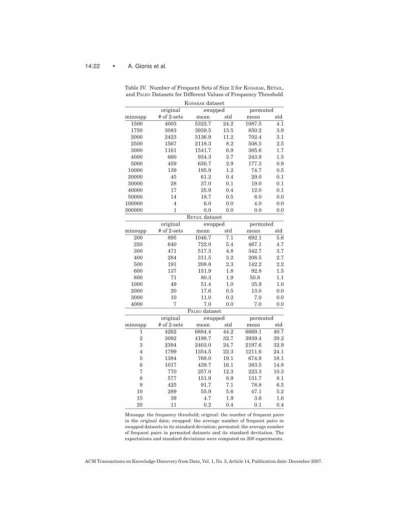
Table IV shows in more detail what happens to the number of frequent pairsin KOSARAK, RETAIL, and PALEO datasets under swap randomizations and per-mutations of the columns, for different values of the frequency threshold. Weobserve for the PALEO dataset that the number of frequent pairs is higher inthe original dataset than in the swapped data for moderate and large valuesof the frequency threshold. This indicates that cooccurrences of variables aremore common in the original data. When the frequency threshold is very small,there are more frequent pairs in the swapped data. The reason for this is thatin the limit, almost every pair tends to occur in the swapped (or permuted)dataset.
For the KOSARAK and RETAIL datasets the results cannot be given for arbitrar-ily small frequencies because the task of finding frequent pairs becomes pro-hibitively expensive. For moderate values of the threshold we observe in bothcases that swapped data has more frequent pairs; the ratios stay remarkablysimilar for different thresholds. Only for the largest threshold in KOSARAK dowe obtain a frequent pair that is more frequent than in the swapped data. Thisbehavior can probably be explained by the existence of disjoint dense blocks of1’s in the data; we have conducted simple experiments and simulations show-ing that in such datasets the behavior of the number of frequent pairs hassuch a trend. We continue the discussion on the behavior of pair frequencies inSection 5.3.
Although the number of frequent itemsets is indicative of the structure thatis contained in the data, it is not informative with respect to what the actualitemsets contained in the collections are, and how the collections relate to eachother. It may well be the case that collections have about the same size, yetare completely disjoint. In the following we present some results on how theitemset collections change under swap randomization. Our results are meantto be indicative of the behavior of the swap randomization, and to help guide
ACM Transactions on Knowledge Discovery from Data, Vol. 1, No. 3, Article 14, Publication date: December 2007.
14:22 • A. Gionis et al.
Table IV. Number of Frequent Sets of Size 2 for KOSARAK, RETAIL,
and PALEO Datasets for Different Values of Frequency Threshold
KOSARAK dataset
original swapped permuted
minsupp # of 2-sets mean std mean std
1500 4003 5322.7 24.2 1087.5 4.1
1750 3083 3939.5 13.5 850.2 3.9
2000 2423 3136.9 11.2 702.4 3.1
2500 1567 2118.3 8.2 508.5 2.5
3000 1161 1541.7 6.9 385.6 1.7
4000 660 934.3 3.7 243.9 1.5
5000 459 630.7 2.9 177.3 0.9
10000 139 195.9 1.2 74.7 0.5
20000 45 61.2 0.4 29.0 0.1
30000 28 37.0 0.1 19.0 0.1
40000 17 25.9 0.4 12.0 0.1
50000 14 18.7 0.5 8.0 0.0
100000 4 6.0 0.0 4.0 0.0
300000 1 0.0 0.0 0.0 0.0
RETAIL dataset
original swapped permuted
minsupp # of 2-sets mean std mean std
200 895 1046.7 7.1 692.1 5.6
250 640 722.0 5.4 467.1 4.7
300 471 517.3 4.8 342.7 3.7
400 284 311.5 3.2 208.5 2.7
500 191 208.8 2.3 142.2 2.2
600 137 151.9 1.8 92.8 1.5
800 71 80.3 1.9 50.8 1.1
1000 49 51.4 1.0 35.9 1.0
2000 20 17.6 0.5 13.0 0.0
3000 10 11.0 0.2 7.0 0.0
4000 7 7.0 0.0 7.0 0.0
PALEO dataset
original swapped permuted
minsupp # of 2-sets mean std mean std
1 4262 6884.4 44.2 6669.1 40.7
2 3092 4198.7 32.7 3939.4 39.2
3 2394 2403.0 24.7 2197.6 32.9
4 1799 1354.5 22.3 1211.6 24.1
5 1384 768.0 19.1 674.9 18.1
6 1017 439.7 16.1 383.5 14.8
7 770 257.0 12.3 223.3 10.3
8 577 151.9 8.9 131.7 8.1
9 425 91.7 7.1 78.8 6.5
10 289 55.9 5.6 47.1 5.2
15 39 4.7 1.9 3.6 1.6
20 11 0.2 0.4 0.1 0.4
Minsupp: the frequency threshold; original: the number of frequent pairs
in the original data; swapped: the average number of frequent pairs in
swapped datasets in its standard deviation; permuted: the average number
of frequent pairs in permuted datasets and its standard devitation. The
expectations and standard deviations were computed on 200 experiments.
ACM Transactions on Knowledge Discovery from Data, Vol. 1, No. 3, Article 14, Publication date: December 2007.
Assessing Data Mining Results via Swap Randomization • 14:23
Table V. Changes in the Collections of Frequent Sets
Dataset |F | |Fs| std |F∩Fs ||F |
|F\Fs ||F |
ABSTRACTS 1128 1004.8 4.8 0.767 0.233
ABSTRACTS′ 4854 839.5 19.2 0.083 0.917
COURSES 9687 442.2 12.5 0.042 0.958
KOSARAK 1436 5644.5 60.8 0.724 0.276
PALEO 2828 266.7 14.8 0.045 0.955
RETAIL 1384 1616.1 12.3 0.882 0.118
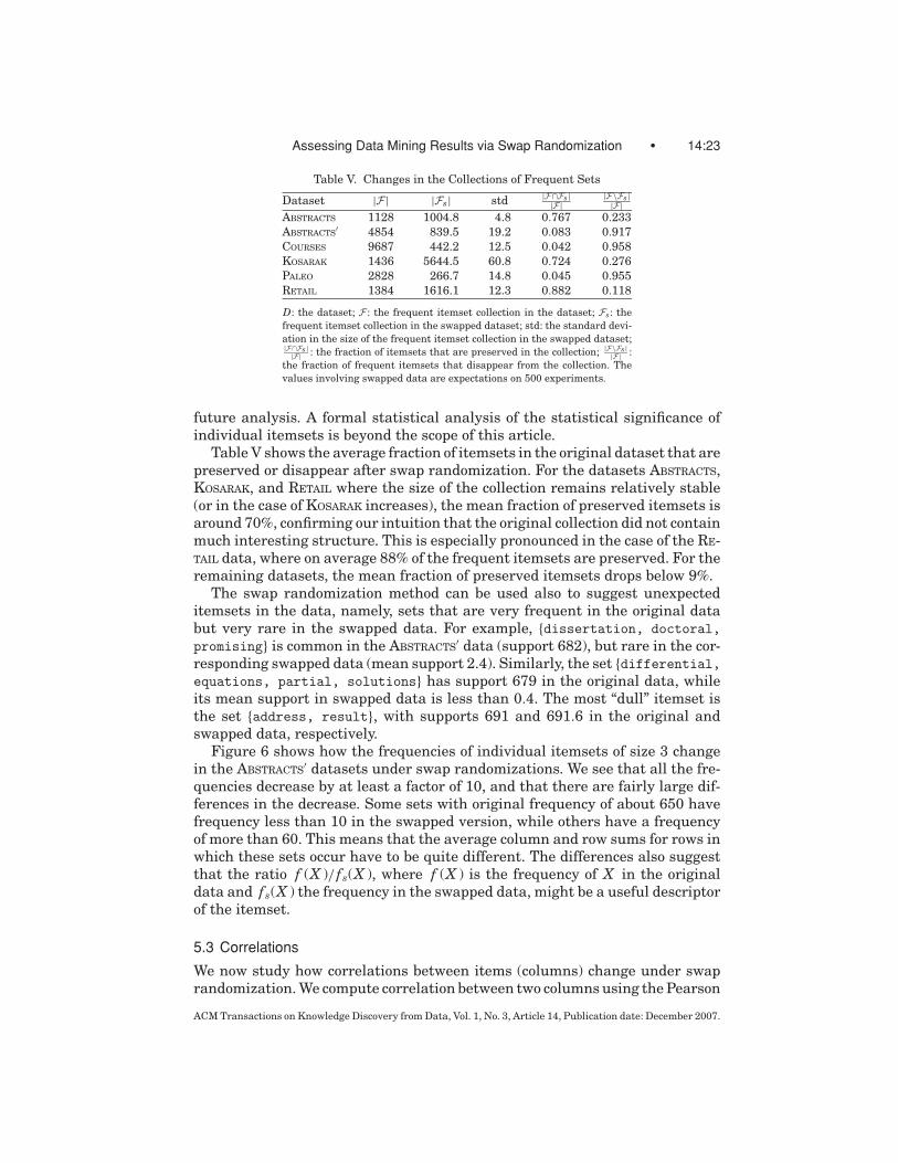
D: the dataset; F : the frequent itemset collection in the dataset; Fs: the
frequent itemset collection in the swapped dataset; std: the standard devi-
ation in the size of the frequent itemset collection in the swapped dataset;|F∩Fs |
|F | : the fraction of itemsets that are preserved in the collection; |F\Fs ||F | :
the fraction of frequent itemsets that disappear from the collection. The
values involving swapped data are expectations on 500 experiments.
future analysis. A formal statistical analysis of the statistical significance ofindividual itemsets is beyond the scope of this article.
Table V shows the average fraction of itemsets in the original dataset that arepreserved or disappear after swap randomization. For the datasets ABSTRACTS,KOSARAK, and RETAIL where the size of the collection remains relatively stable(or in the case of KOSARAK increases), the mean fraction of preserved itemsets isaround 70%, confirming our intuition that the original collection did not containmuch interesting structure. This is especially pronounced in the case of the RE-TAIL data, where on average 88% of the frequent itemsets are preserved. For theremaining datasets, the mean fraction of preserved itemsets drops below 9%.
The swap randomization method can be used also to suggest unexpecteditemsets in the data, namely, sets that are very frequent in the original databut very rare in the swapped data. For example, {dissertation, doctoral,promising} is common in the ABSTRACTS
′ data (support 682), but rare in the cor-responding swapped data (mean support 2.4). Similarly, the set {differential,equations, partial, solutions} has support 679 in the original data, whileits mean support in swapped data is less than 0.4. The most “dull” itemset isthe set {address, result}, with supports 691 and 691.6 in the original andswapped data, respectively.
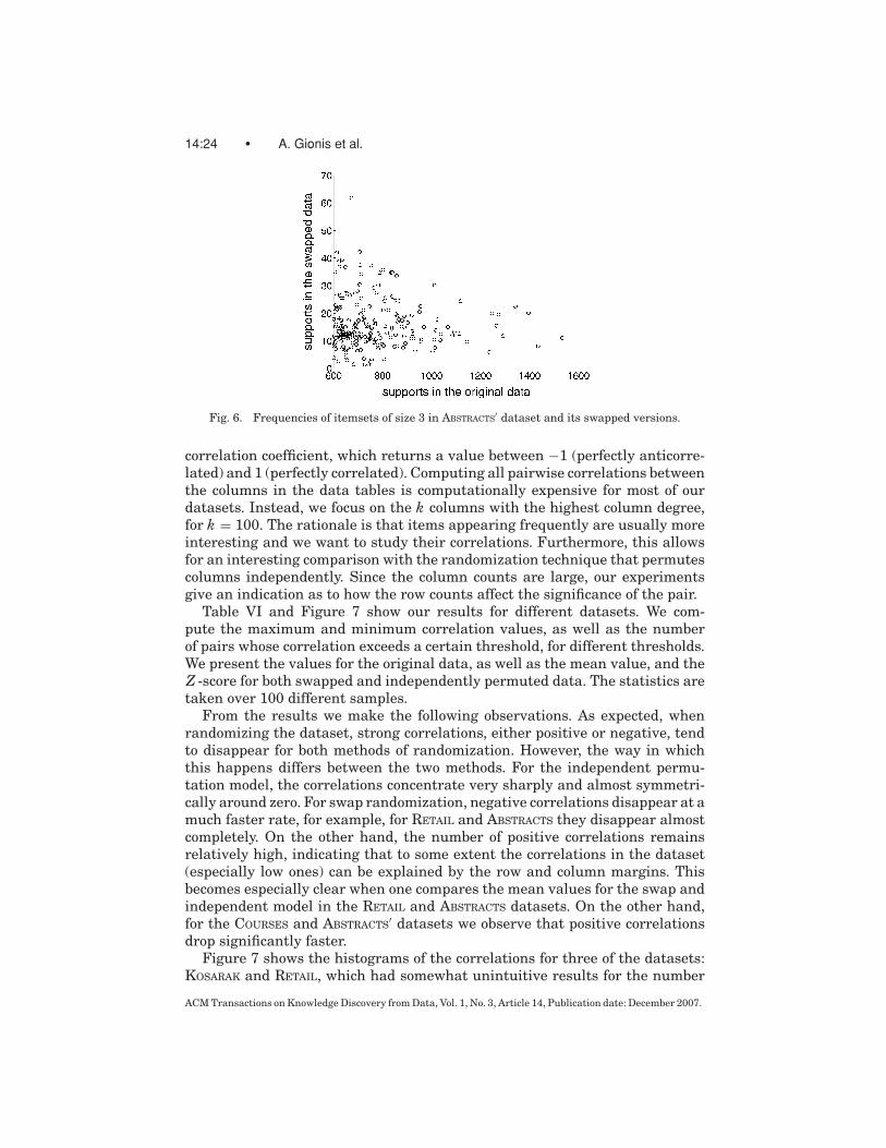
Figure 6 shows how the frequencies of individual itemsets of size 3 changein the ABSTRACTS
′ datasets under swap randomizations. We see that all the fre-quencies decrease by at least a factor of 10, and that there are fairly large dif-ferences in the decrease. Some sets with original frequency of about 650 havefrequency less than 10 in the swapped version, while others have a frequencyof more than 60. This means that the average column and row sums for rows inwhich these sets occur have to be quite different. The differences also suggestthat the ratio f (X )/ fs(X ), where f (X ) is the frequency of X in the originaldata and fs(X ) the frequency in the swapped data, might be a useful descriptorof the itemset.
5.3 Correlations
We now study how correlations between items (columns) change under swaprandomization. We compute correlation between two columns using the Pearson
ACM Transactions on Knowledge Discovery from Data, Vol. 1, No. 3, Article 14, Publication date: December 2007.
14:24 • A. Gionis et al.
Fig. 6. Frequencies of itemsets of size 3 in ABSTRACTS′ dataset and its swapped versions.
correlation coefficient, which returns a value between −1 (perfectly anticorre-lated) and 1 (perfectly correlated). Computing all pairwise correlations betweenthe columns in the data tables is computationally expensive for most of ourdatasets. Instead, we focus on the k columns with the highest column degree,for k = 100. The rationale is that items appearing frequently are usually moreinteresting and we want to study their correlations. Furthermore, this allowsfor an interesting comparison with the randomization technique that permutescolumns independently. Since the column counts are large, our experimentsgive an indication as to how the row counts affect the significance of the pair.
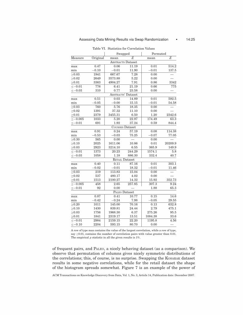
Table VI and Figure 7 show our results for different datasets. We com-pute the maximum and minimum correlation values, as well as the numberof pairs whose correlation exceeds a certain threshold, for different thresholds.We present the values for the original data, as well as the mean value, and theZ -score for both swapped and independently permuted data. The statistics aretaken over 100 different samples.
From the results we make the following observations. As expected, whenrandomizing the dataset, strong correlations, either positive or negative, tendto disappear for both methods of randomization. However, the way in whichthis happens differs between the two methods. For the independent permu-tation model, the correlations concentrate very sharply and almost symmetri-cally around zero. For swap randomization, negative correlations disappear at amuch faster rate, for example, for RETAIL and ABSTRACTS they disappear almostcompletely. On the other hand, the number of positive correlations remainsrelatively high, indicating that to some extent the correlations in the dataset(especially low ones) can be explained by the row and column margins. Thisbecomes especially clear when one compares the mean values for the swap andindependent model in the RETAIL and ABSTRACTS datasets. On the other hand,for the COURSES and ABSTRACTS
′ datasets we observe that positive correlationsdrop significantly faster.
Figure 7 shows the histograms of the correlations for three of the datasets:KOSARAK and RETAIL, which had somewhat unintuitive results for the number
ACM Transactions on Knowledge Discovery from Data, Vol. 1, No. 3, Article 14, Publication date: December 2007.
Assessing Data Mining Results via Swap Randomization • 14:25
Table VI. Statistics for Correlation Values
Swapped Permuted
Measure Original mean Z mean ZABSTRACTS Dataset
max 0.47 0.06 11.19 0.01 514.2
min −0.10 −0.01 11.90 −0.01 137.5
≥0.03 1941 667.67 7.28 0.00 —
≥0.02 2649 3573.88 5.22 0.00 —
≥0.01 3363 4904.27 7.91 0.86 3342
≤−0.01 776 6.41 21.19 0.66 775
≤−0.03 310 0.77 23.58 0.00 —
ABSTRACTS′ Dataset
max 0.51 0.03 14.89 0.01 592.5
min −0.05 −0.00 15.15 −0.01 54.58
≥0.03 760 5.76 18.35 0.00 —
≥0.02 1391 37.32 11.10 0.00 —
≥0.01 2379 3455.31 6.50 1.20 2342.6
≤−0.005 1033 5.20 22.97 174.49 63.3
≤−0.01 691 1.92 37.24 0.59 844.4
COURSES Dataset
max 0.91 0.24 57.19 0.08 114.38
min −0.53 −0.03 75.25 −0.07 77.05
≥0.30 565 0.00 — 0.00 —
≥0.10 2025 1611.06 10.86 0.01 20209.9
≥0.03 2923 3214.10 6.55 365.9 149.9
≤−0.01 1373 20.23 244.29 1574.1 5.8
≤−0.03 1058 1.18 886.30 332.4 40.7
RETAIL Dataset
max 0.40 0.11 87.16 0.01 303.1
min −0.02 −0.01 18.32 −0.01 11.46
≥0.03 219 113.83 15.04 0.00 —
≥0.02 537 480.17 4.02 0.00 —
≥0.01 1513 2100.27 14.32 15.92 352.73
≤−0.005 458 2.65 257.85 307.3 9.24
≤−0.01 92 0.00 — 1.88 65.3
PALEO Dataset
max 0.87 0.41 10.77 0.15 14.6
min −0.42 −0.24 7.98 −0.05 29.55
≥0.20 1011 145.00 70.16 0.13 632.8
≥0.10 1430 839.81 24.44 2.79 475.1
≥0.03 1756 1968.30 6.37 275.26 95.5
≥0.01 1841 2319.17 13.51 1084.38 33.6
≤−0.01 2984 2159.15 22.20 1195.8 4.56
≤−0.10 2204 593.15 80.70 0.00 —
A row of type max contains the value of the largest correlation, while a row of type,
say ≥0.01, contains the number of correlation pairs with value greater than 0.01.
The empirical p statistic in all the given results is 1%.
of frequent pairs, and PALEO, a nicely behaving dataset (as a comparison). Weobserve that permutation of columns gives nicely symmetric distributions ofthe correlations; this, of course, is no surprise. Swapping the KOSARAK datasetresults in some negative correlations, while for the retail dataset the shapeof the histogram spreads somewhat. Figure 7 is an example of the power of
ACM Transactions on Knowledge Discovery from Data, Vol. 1, No. 3, Article 14, Publication date: December 2007.
14:26 • A. Gionis et al.
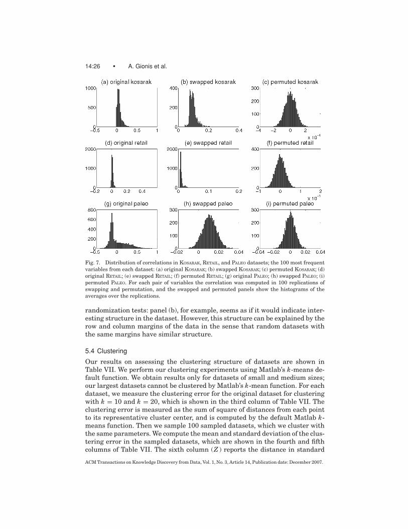
Fig. 7. Distribution of correlations in KOSARAK, RETAIL, and PALEO datasets; the 100 most frequent
variables from each dataset: (a) original KOSARAK; (b) swapped KOSARAK; (c) permuted KOSARAK; (d)
original RETAIL; (e) swapped RETAIL; (f) permuted RETAIL; (g) original PALEO; (h) swapped PALEO; (i)
permuted PALEO. For each pair of variables the correlation was computed in 100 replications of
swapping and permutation, and the swapped and permuted panels show the histograms of the
averages over the replications.
randomization tests: panel (b), for example, seems as if it would indicate inter-esting structure in the dataset. However, this structure can be explained by therow and column margins of the data in the sense that random datasets withthe same margins have similar structure.
5.4 Clustering
Our results on assessing the clustering structure of datasets are shown inTable VII. We perform our clustering experiments using Matlab’s k-means de-fault function. We obtain results only for datasets of small and medium sizes;our largest datasets cannot be clustered by Matlab’s k-mean function. For eachdataset, we measure the clustering error for the original dataset for clusteringwith k = 10 and k = 20, which is shown in the third column of Table VII. Theclustering error is measured as the sum of square of distances from each pointto its representative cluster center, and is computed by the default Matlab k-means function. Then we sample 100 sampled datasets, which we cluster withthe same parameters. We compute the mean and standard deviation of the clus-tering error in the sampled datasets, which are shown in the fourth and fifthcolumns of Table VII. The sixth column (Z ) reports the distance in standard
ACM Transactions on Knowledge Discovery from Data, Vol. 1, No. 3, Article 14, Publication date: December 2007.
Assessing Data Mining Results via Swap Randomization • 14:27
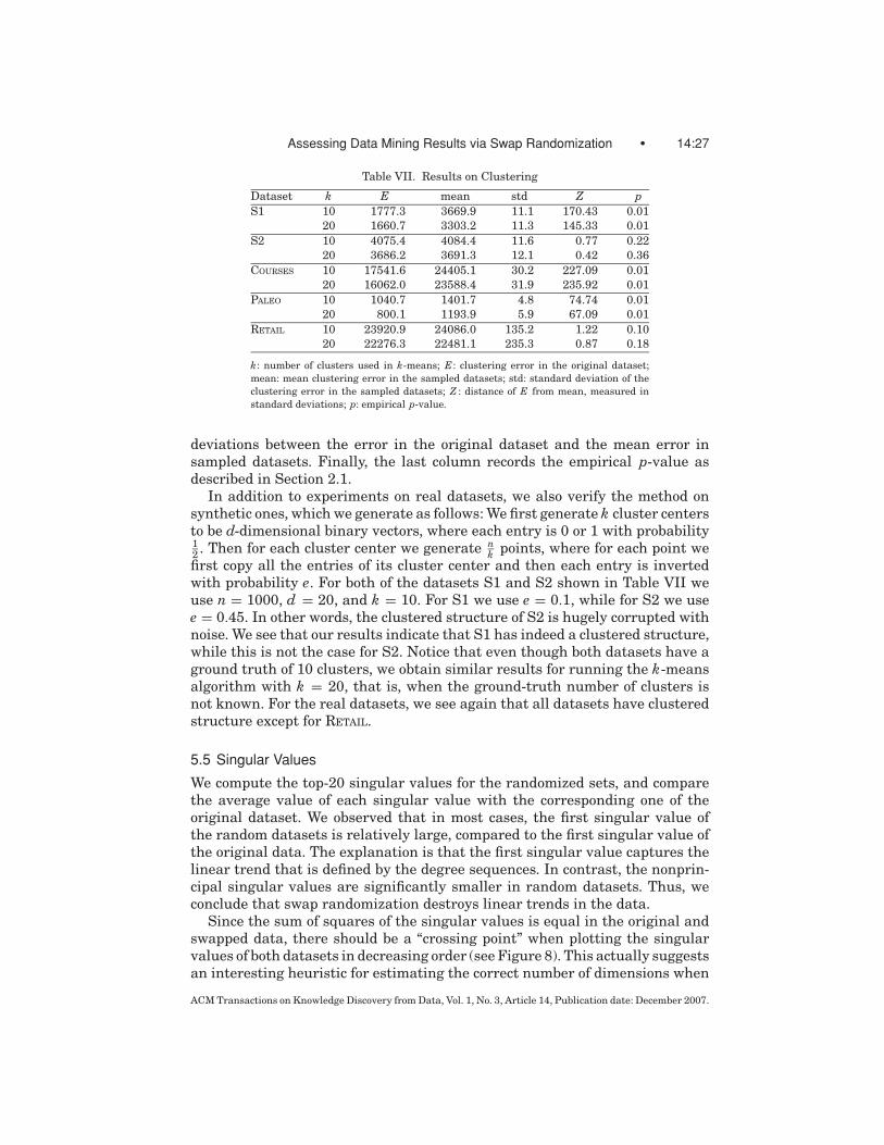
Table VII. Results on Clustering
Dataset k E mean std Z pS1 10 1777.3 3669.9 11.1 170.43 0.01
20 1660.7 3303.2 11.3 145.33 0.01
S2 10 4075.4 4084.4 11.6 0.77 0.22
20 3686.2 3691.3 12.1 0.42 0.36
COURSES 10 17541.6 24405.1 30.2 227.09 0.01
20 16062.0 23588.4 31.9 235.92 0.01
PALEO 10 1040.7 1401.7 4.8 74.74 0.01
20 800.1 1193.9 5.9 67.09 0.01
RETAIL 10 23920.9 24086.0 135.2 1.22 0.10
20 22276.3 22481.1 235.3 0.87 0.18
k: number of clusters used in k-means; E: clustering error in the original dataset;
mean: mean clustering error in the sampled datasets; std: standard deviation of the
clustering error in the sampled datasets; Z : distance of E from mean, measured in
standard deviations; p: empirical p-value.
deviations between the error in the original dataset and the mean error insampled datasets. Finally, the last column records the empirical p-value asdescribed in Section 2.1.
In addition to experiments on real datasets, we also verify the method onsynthetic ones, which we generate as follows: We first generate k cluster centersto be d-dimensional binary vectors, where each entry is 0 or 1 with probability12. Then for each cluster center we generate n
k points, where for each point wefirst copy all the entries of its cluster center and then each entry is invertedwith probability e. For both of the datasets S1 and S2 shown in Table VII weuse n = 1000, d = 20, and k = 10. For S1 we use e = 0.1, while for S2 we usee = 0.45. In other words, the clustered structure of S2 is hugely corrupted withnoise. We see that our results indicate that S1 has indeed a clustered structure,while this is not the case for S2. Notice that even though both datasets have aground truth of 10 clusters, we obtain similar results for running the k-meansalgorithm with k = 20, that is, when the ground-truth number of clusters isnot known. For the real datasets, we see again that all datasets have clusteredstructure except for RETAIL.
5.5 Singular Values
We compute the top-20 singular values for the randomized sets, and comparethe average value of each singular value with the corresponding one of theoriginal dataset. We observed that in most cases, the first singular value ofthe random datasets is relatively large, compared to the first singular value ofthe original data. The explanation is that the first singular value captures thelinear trend that is defined by the degree sequences. In contrast, the nonprin-cipal singular values are significantly smaller in random datasets. Thus, weconclude that swap randomization destroys linear trends in the data.
Since the sum of squares of the singular values is equal in the original andswapped data, there should be a “crossing point” when plotting the singularvalues of both datasets in decreasing order (see Figure 8). This actually suggestsan interesting heuristic for estimating the correct number of dimensions when
ACM Transactions on Knowledge Discovery from Data, Vol. 1, No. 3, Article 14, Publication date: December 2007.
14:28 • A. Gionis et al.
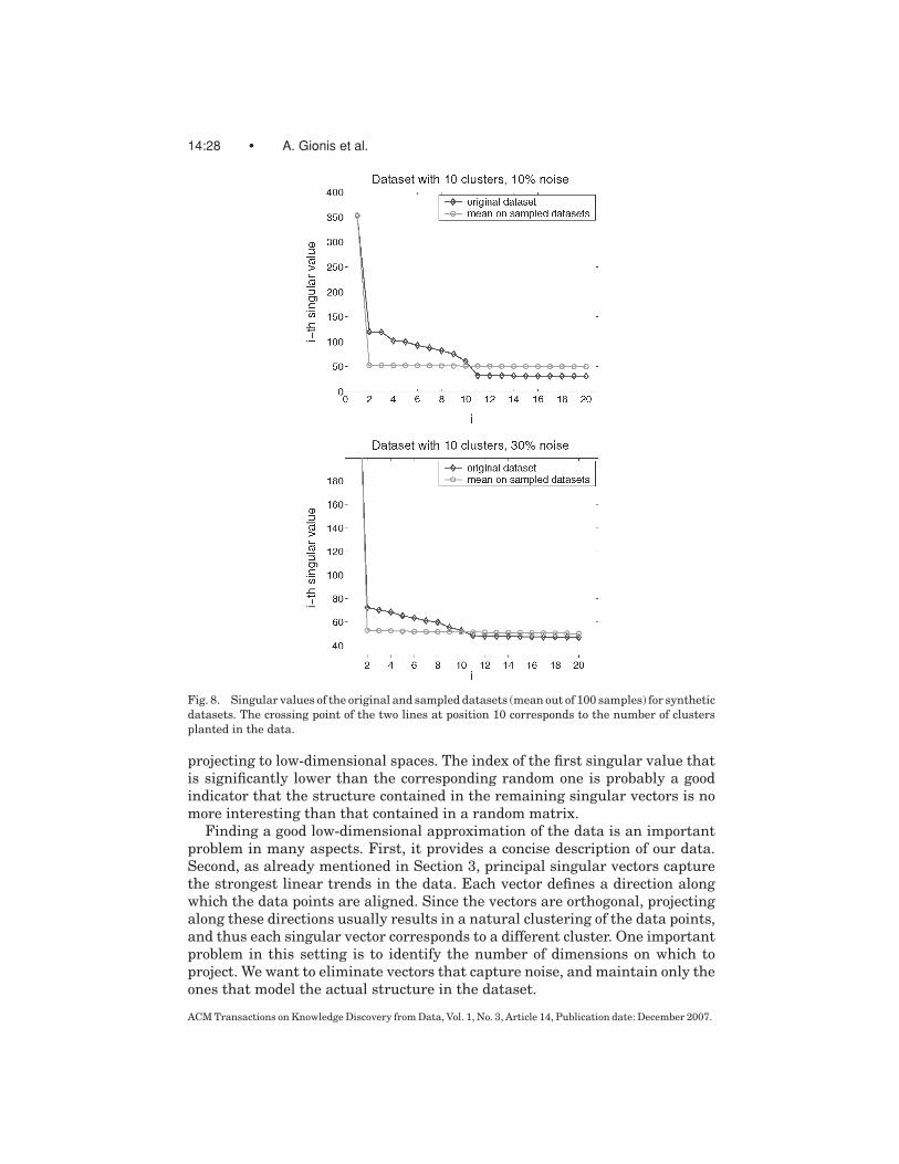
Fig. 8. Singular values of the original and sampled datasets (mean out of 100 samples) for synthetic
datasets. The crossing point of the two lines at position 10 corresponds to the number of clusters
planted in the data.
projecting to low-dimensional spaces. The index of the first singular value thatis significantly lower than the corresponding random one is probably a goodindicator that the structure contained in the remaining singular vectors is nomore interesting than that contained in a random matrix.
Finding a good low-dimensional approximation of the data is an importantproblem in many aspects. First, it provides a concise description of our data.Second, as already mentioned in Section 3, principal singular vectors capturethe strongest linear trends in the data. Each vector defines a direction alongwhich the data points are aligned. Since the vectors are orthogonal, projectingalong these directions usually results in a natural clustering of the data points,and thus each singular vector corresponds to a different cluster. One importantproblem in this setting is to identify the number of dimensions on which toproject. We want to eliminate vectors that capture noise, and maintain only theones that model the actual structure in the dataset.
ACM Transactions on Knowledge Discovery from Data, Vol. 1, No. 3, Article 14, Publication date: December 2007.

Assessing Data Mining Results via Swap Randomization • 14:29
We observe that in many cases the crossing point in the singular-valuesplot can help guide this decision. For example, the PALEO data is conjectured tocontain three clusters and the crossing point for this data is indeed at position 3.We experiment further with the aforementioned idea on synthetic data in whichwe can plant a known number of clusters. The data was generated with theprocedure described in the previous section. Note that in the case where nonoise is added in the data generation, the number of singular vectors is equal tothe number of planted clusters. The addition of noise does not add structure, sowe expect the new singular values to be insignificant according to our measure.Figure 8 shows indeed that for a dataset with 10 clusters, the crossing point isat position 10, for noise levels ranging from 10% to as high as 30%.
6. RELATED WORK AND ADDITIONAL COMMENTS
Defining the significance of discovered patterns has attracted a lot of attentionin data mining. In one of the first known papers, Brin et al. [1997] consideredmeasuring the significance of associations via the chi-square test. A lot of othermeasures have been proposed to capture the interestingness of patterns, suchas DuMouchel and Pregibon [2001], Jaroszewicz and Simovici [2001], Liu et al.[2001, 1999], Megiddo and Srikant [1998], and Xiong et al. [2004]. Megiddoand Srikant [1998] use ideas from statistical significance testing to estimatethe number of false discoveries and rank the set of the association rules found.Liu et al. [2001] present an algorithm to identify “nonactionable” associationrules, that is, rules that are significant but covered by other, more specific rules.DeMouchel and Pregibon [2001] apply statistical filtering for association rulesusing a Bayesian framework. Recently, Webb [2007, 2006] built upon some ofthe existing approaches and presented two generic approaches for discoveringsignificant rules while filtering false discoveries. A comprehensive presentationand comparison of the methods that capture interestingness of patterns can befound in Tan et al. [2002].
The problem is also very well studied in statistics, and there is a significantamount of work for sampling from the space of contingency tables [Chen et al.2005; Cobb and Chen 2003; Diaconis and Gangolli 1995; Snijders 1991], as wellas several studies that give asymptotics on the exact number of such tables,such as Wang and Zhang [1998]. The algorithmic properties of some of thesemethods are discussed in Bezakova et al. [2006]. A good survey on the topic isprovided by Chen et al. [2005].
In theoretical computer science the subject has drawn attention in the con-text of providing bounds for the mixing of the Markov chain. Very recently,Bezakova et al. [2006] gave a polynomial-time algorithm for sampling binary0–1 matrices with given margins. The algorithm is based on a different Markovchain than that based on swaps.
The problem of generating random matrices with fixed margins has also beenstudied in many application areas, such as ecology [Sanderson 2000] and biol-ogy [Kashtan et al. 2004], and analysis of complex networks [Milo et al. 2002].
In using the swap randomization framework, Di is obtained from D by mak-ing a sequence of swaps. As a single swap has only very limited effect on the
ACM Transactions on Knowledge Discovery from Data, Vol. 1, No. 3, Article 14, Publication date: December 2007.
14:30 • A. Gionis et al.
dataset, one might look for implementations of A that take advantage of theincremental characteristics of the datasets for which A is being used. This isfairly straightforward, for example, for frequent sets, but we have not pursuedthis idea further.
Finally, we remark that it is possible to directly generate random datasetsthat do not preserve exact row and column sums but on expectation. This in-volves setting each entry (i, j ) equal to 1 with probability ric j /L, and equal to 0otherwise. This expectation model has the drawback that the fraction ric j /L hasprobability interpretation only if max{ri, c j } ≤ L. The advantage of this modelis that the generation process has fixed complexity (quadratic), which is likelyfaster than the Metropolis-Hasting algorithm. Furthermore, it is amenable toformal analysis. Experimenting with this model, we found that it gives similarresults as the swap method, but sometimes is slightly inaccurate. For instance,such inaccuracies were observed in the KOSARAK dataset in which both the rowand column sums follow power-law distribution. Additionally, the savings inrunning time are not significant.
7. CONCLUSIONS
We have studied the algorithmic properties of swap randomization, and de-scribed how it can be used in assessing results of data mining algorithms. Wegave an algorithmic treatment of the swap randomization method, showingsome results on the computation of the number of immediately reachable statesin the Markov chain, and we showed that the Self loop algorithm is alwaysmore efficient than the Metropolis-Hastings method for this problem. Ourwork shows that swap randomization is efficient in practice, and that it can beused for large datasets.
We have conducted extensive experiments on the use of swap randomization.The results show large differences in the amount of structure that is presentin different datasets. For example, when viewed through clustering or frequentsets, the RETAIL dataset apparently has very little structure, apart from its veryskewed degree distribution for columns and (slightly less) for rows. The num-ber of frequent sets in the real dataset is about the same as in the randomizedversions, and clustering the original and randomized versions yields about thesame error. On the other hand, several of the other datasets clearly have lotsof second-order structure, as evidenced by the dramatic drop in number of fre-quent sets and strong correlations when moving to the randomized version ofthe data.
Swap randomization is a technique that maintains the first-order statistics ofthe data. Thus, it should not be used to study the significance of discoveries thatdepend only on the first-order statistics of the data, namely, the row and columnmargins; power laws are an example of these types of statistics. An interestingquestion is whether it is possible to generate, from a dataset D, random datasetshaving the same margins as D while keeping also some second-order statistics(e.g., the frequency of certain variable pairs) fixed. It can be shown that onecan indeed efficiently generate datasets that have the given row and columnmargins, and additionally maintain counts { f (X i)}, where the sets X i are pairs
ACM Transactions on Knowledge Discovery from Data, Vol. 1, No. 3, Article 14, Publication date: December 2007.
Assessing Data Mining Results via Swap Randomization • 14:31
and the collection {X i} is acyclic. Maintaining frequencies of sets in general isNP-hard [Mielikainen 2003; Calders 2004].
There are also other types of statistics that might be interesting to maintainin 0–1 data. We have already remarked on the possibility of maintaining thecounts approximately. Another option would be to maintain the counts of smallsubgraphs, such as cliques K2,2 or K2,3 [Tomkins 2006].
Availability. Software for swap randomization can be found at http://www.cs.helsinki.fi/hiit bru/software/swaps/.
ACKNOWLEDGMENTS
We thank Jean-Francois Boulicaut, Celine Robardet, and Jeremy Besson forinteresting discussions that got us started on swaps, and Dimitris Achlioptasand Andrew Tomkins for useful remarks.
REFERENCES
BESAG, J. 2004. Markov chain Monte Carlo methods for statistical inference. http://www.ims.
nus.edu.sg/Programs/mcmc/files/besag tl.pdf.
BESAG, J. AND CLIFFORD, P. 1989. Generalized Monte Carlo significance tests. Biometrika 76, 4,
633–642.
BESAG, J. AND CLIFFORD, P. 1991. Sequential Monte Carlo p-values. Biometrika 78, 2, 301–304.
BEZAKOVA, I., BHATNAGAR, N., AND VIGODA, E. 2006. Sampling binary contingency tables with a
greedy start. In Proceedings of the 17th Annual ACM-SIAM Symposium on Discrete Algorithms(SODA), SIAM, 414–423.
BEZAKOVA, I., SINCLAIR, A., STEFANKOVIC, D., AND VIGODA, E. 2006. Negative examples for sequential
importance sampling of binary contingency tables. http://arxiv.org/abs/math.ST/0606650.
BRIJS, T., SWINNEN, G., VANHOOF, K., AND WETS, G. 1999. Using association rules for product assort-
ment decisions: A case study. In Proceedings of the 5th ACM SIGKDD International Conferenceon Knowledge Discovery and Data Mining, San Diego, CA, 254–260.
BRIN, S., MOTWANI, R., AND SILVERSTEIN, C. 1997. Beyond market baskets: Generalizing association
rules to correlations. In Proceedings of the ACM SIGMOD International Conference on Manage-ment of Data, Tucson, AZ, 265–276.
CALDERS, T. 2004. Computational complexity of itemset frequency satisfiability. In Proceedingsof the 23rd ACM SIGMOD-SIGACT-SIGART Symposium on Principles of Database Systems,
143–154.
CHEN, Y., DIACONIS, P., HOLMES, S. P., AND LIU, J. S. 2005. Sequential Monte Carlo methods for
statistical analysis of tables. J. Amer. Statis. Assoc. 100, 469, 109–120.
COBB, G. W. AND CHEN, Y.-P. 2003. An application of Markov chain Monte Carlo to community
ecology. Amer. Math. Month. 110, 264–288.
DIACONIS, P. AND GANGOLLI, A. 1995. Rectangular arrays with fixed margins. In Discrete Proba-bility and Algorithms, 15–41.
DIACONIS, P. AND SALOFF-COSTE, L. 1995. Random walk on contingency tables with fixed row and
column sums. Tech. Rep., Department of Mathematics, Harvard University.
DUMOUCHEL, W. AND PREGIBON, D. 2001. Empirical Bayes screening for multi-item associations.
In Knowledge Discovery and Data Mining, 67–76.
DYER, M. 2003. Approximate counting by dynamic programming. In Proceedings of the 35thAnnual ACM Symposium on Theory of Computing, San Diego, CA, 693–699.
FORTELIUS, M. 2006. Neogene of the old world database of fossil mammals (NOW). http://www.
helsinki.fi/science/now/.
GOOD, P. 2000. Permutation Tests: A Practical Guide to Resampling Methods for Testing Hypothe-ses. Springer.
HASTINGS, W. K. 1970. Monte Carlo sampling methods using Markov chains and their applica-
tions. Biometrika 57, 1, 97–109.
ACM Transactions on Knowledge Discovery from Data, Vol. 1, No. 3, Article 14, Publication date: December 2007.
14:32 • A. Gionis et al.
JAROSZEWICZ, S. AND SIMOVICI, D. A. 2001. A general measure of rule interestingness. In Proceed-ings of the 5th European Conference on Principles of Data Mining and Knowledge Discovery(PKDD), 253–265.
KASHTAN, N., ITZKOVITZ, S., MILO, R., AND ALON, U. 2004. Efficient sampling algorithm for estimating
dubgraph concentrations and detecting network motifs. Bioinf. 20, 11, 1746–1758.
LIU, B., HSU, W., AND MA, Y. 1999. Pruning and summarizing the discovered associations. In
Proceedings of the 5th ACM SIGKDD International Conference on Knowledge Discovery andData Mining, San Diego, CA, 125–134.
LIU, B., HSU, W., AND MA, Y. 2001. Identifying non-actionable association rules. In KnowledgeDiscovery and Data Mining, 329–334.
MEGIDDO, N. AND SRIKANT, R. 1998. Discovering predictive association rules. In Proceedings ofthe 4th International Conference on Knowledge Discovery and Data Mining (KDD), New York,
274–278.
METROPOLIS, N., ROSENBLUTH, A., ROSENBLUTH, M., TELLER, A., AND TELLER, E. 1953. Equations of
state calculations by fast computing machines. J. Chem. Phys. 21, 1087–1092.
MIELIKAINEN, T. 2003. On inverse frequent set mining. In Proceedings of the 2nd Workshop onPrivacy Preserving Data Mining (PPDM), IEEE Computer Society, 18–23.
MILO, R., SHEN-ORR, S., ITZKOVIRZ, S., KASHTAN, N., CHKLOVSKII, D., AND ALON, U. 2002. Network
motifs: Simple building blocks of complex networks. Sci. 298, 824–827.
NEWMAN, M. 2003. The structure and function of complex networks. SIAM Rev. 45, 2, 167–256.
RYSER, H. J. 1957. Combinatorial properties of matrices of zeros and ones. Canadian J. Math. 9,
371–377.
SANDERSON, J. 2000. Testing ecological patterns. Amer. Sci. 88, 332–339.
SNIJDERS, F. 1991. Enumeration and simulation methods for 0–1 matrices with given marginals.
Psychometrika 56, 397–417.
TAN, P.-N., KUMAR, V., AND SRIVASTAVA, J. 2002. Selecting the right interestingness measure for
association patterns. In Proceedings of the 8th ACM SIGKDD International Conference on Knowl-edge Discovery and Data Mining, Edmonton, Alberta, Canada, 32–41.
TOMKINS, A. 2006. Private communication.
WANG, B. Y. AND ZHANG, F. 1998. Precise number of (0, 1)-matrices in u(r, s). Discrete Math. 187,
211–220.
WEBB, G. 2006. Discovering significant rules. In Proceedings of the 12th ACM SIGKDD Interna-tional Conference on Knowledge Discovery and Data Mining, 434–443.
WEBB, G. 2007. Discovering significant patterns. Mach. Learn., to appear.
XIONG, H., SHEKHAR, S., TAN, P.-N., AND KUMAR, V. 2004. Exploiting a support-based upper bound
of pearson’s correlation coefficient for efficiently identifying strongly correlated pairs. In Pro-ceedings of the 10th ACM SIGKDD International Conference on Knowledge Discovery and DataMining, Seattle, WA, 334–343.
Received January 2007; revised June 2007; accepted July 2007
ACM Transactions on Knowledge Discovery from Data, Vol. 1, No. 3, Article 14, Publication date: December 2007.