Assembly System

8/6/2019 Assembly System

http://slidepdf.com/reader/full/assembly-system 1/16

Optimal Inventory Policies for Assembly Systems under Random Demands

Author(s): Kaj RoslingSource: Operations Research, Vol. 37, No. 4 (Jul. - Aug., 1989), pp. 565-579Published by: INFORMSStable URL: http://www.jstor.org/stable/171257 .

Accessed: 12/05/2011 10:50

Your use of the JSTOR archive indicates your acceptance of JSTOR's Terms and Conditions of Use, available at .http://www.jstor.org/page/info/about/policies/terms.jsp. JSTOR's Terms and Conditions of Use provides, in part, that unless

you have obtained prior permission, you may not download an entire issue of a journal or multiple copies of articles, and you

may use content in the JSTOR archive only for your personal, non-commercial use.

Please contact the publisher regarding any further use of this work. Publisher contact information may be obtained at .http://www.jstor.org/action/showPublisher?publisherCode=informs. .

Each copy of any part of a JSTOR transmission must contain the same copyright notice that appears on the screen or printed

page of such transmission.

JSTOR is a not-for-profit service that helps scholars, researchers, and students discover, use, and build upon a wide range of

content in a trusted digital archive. We use information technology and tools to increase productivity and facilitate new forms

of scholarship. For more information about JSTOR, please contact [email protected].

INFORMS is collaborating with JSTOR to digitize, preserve and extend access to Operations Research.

http://www.jstor.org/action/showPublisher?publisherCode=informs

http://www.jstor.org/stable/171257?origin=JSTOR-pdf

http://www.jstor.org/page/info/about/policies/terms.jsp



http://www.jstor.org/page/info/about/policies/terms.jsp

http://www.jstor.org/stable/171257?origin=JSTOR-pdf




OPTIMAL NVENTORY OLICIESFOR ASSEMBLYSYSTEMSUNDER RANDOMDEMANDS

KAJ ROSLINGLinkoping Institute of Technology, Linkoping, Sweden

(Received March 1987; revision received December 1987; accepted April 1988)

This paper considers an inventory model of an assembly system with random demands and proportional costs of

production and stock holding activities. The model is a generalization of the facilities in series model of Clark and Scarf.

Under an assumption on the initial stock levels that in any case should appear in the long run (Long-Run Balance), it is

demonstrated that the assembly system can be remodeled as a series system. Hence, simple reorder policies are optimal

and the computational requirements are drastically reduced. Simple approximate policies are suggested for the generally

short period of time when systems might be out of long-run balance. There is some discussion of extensions.

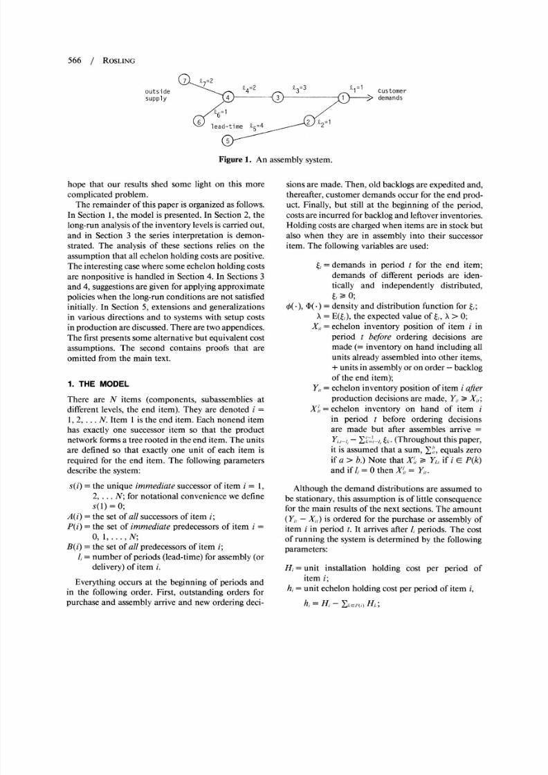
T his paper examines a periodic review, infinite

horizon model of an assembly inventory system

with proportionalcosts of production. In an assemblysystem, a number of components acquired from out-

side vendorsareassembled, typicallyin several stages,into subassembliesand then, finally, into a single end

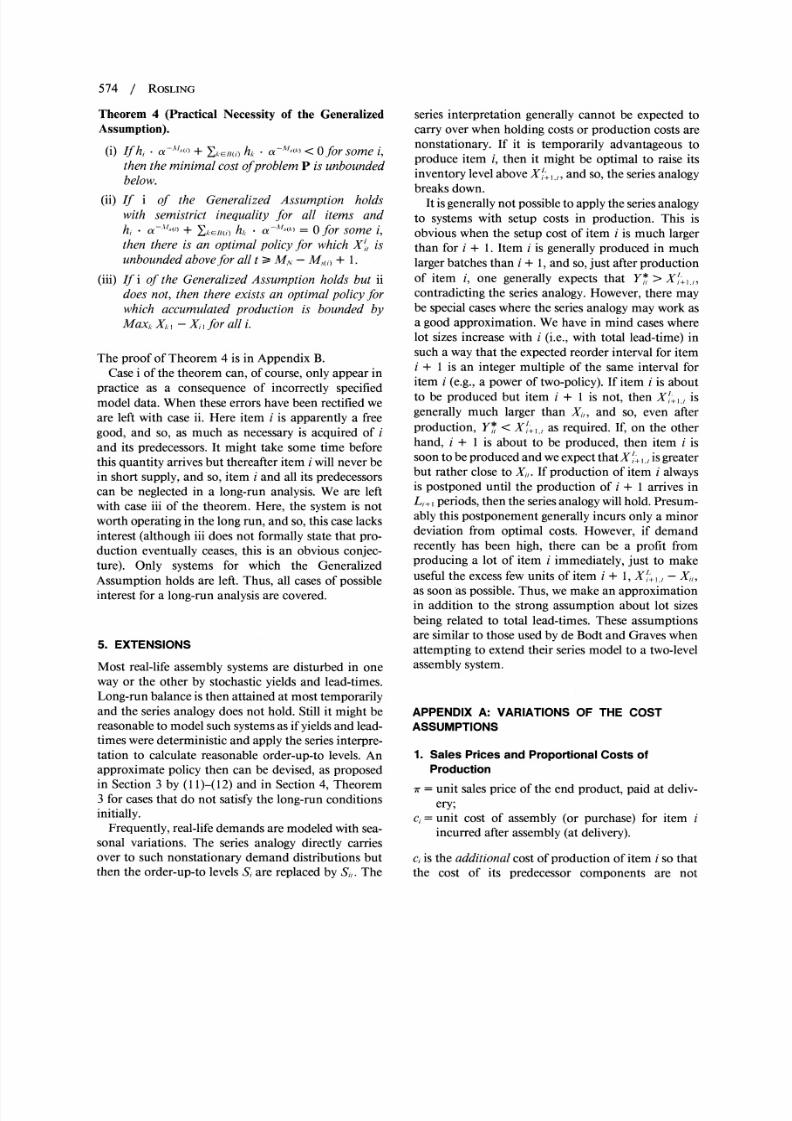
product. A generic system is depicted in Figure 1. In

each period, production orders are made for all items.The ordered amounts are available after a fixed lead-

time, and are then held in stock until assembled into

other items or demanded by customers.The randomcustomer demands occur only for the end productand unsatisfied demands arebacklogged.

The present model is a direct generalization of the

initial work on multiechelon inventory theory due to

Clarkand Scarf (1960). They found an efficient wayto compute an optimal ordering policy for a pureseries system and suggested an approximate way to

handle distributivesystems, i.e., systems wherea cen-

traldepot serves severalretailers.Fukuda (1961) gen-eralized the approachto allow for disposal of stocks.

The work of Clark and Scarf was computationally

streamlined and generalized to the stationaryinfinitehorizon case by Federgruen and Zipkin (1984).Rosling (1989) derived bounds on the optimal reorderlevels. A similarseries model under continuous reviewhas been investigated by Axsater and Lundell (1984).

General multilocation inventory problems withproportional costs have been studied by Bessler andVeinott (1966) and Karmarkar(1981, 1987). They

obtained simple form optimal policies under the

restrictive assumption that all lead-times equal zero.Schmidt and Nahmias (1985) investigated a finite

horizon model of two components assembled into a

single end product. They derived a complicated opti-

mal policy under general assumptions on lead-timesand initial stock levels.

In the present paper,we derive optimal policies for

general assembly systems under a restriction on the

initial stock levels. Our interest is limited to those

stock levels that can prevail n the long run for systems

run by optimal or otherwise reasonable policies.

Under this initial condition, it turns out that the

assembly system can be interpretedas a seriessystem,and hence, there is a simple optimal policy that can

be calculatedconveniently by Clarkand Scarf's (1960)

approach.This result contrastsmost encouragingly o

the computational intractabilityof a generallyoptimal

policy.The assumed absence of setup costs in production

limits the applicability of the present model. The

inclusion of such costs in stochastic multiechelon

inventory models is extremely difficult, however.

Clark and Scarf (1962) attempted to include setup

costs in their series model, but they were only able to

derive upper and lower bounds on the minimal cost.Their approachwas extendedto distributivestructures

by Hochstadter(1970) and Rosling (1977). As far as

we know, therehas been no substantialcomputationaltest of this approximateapproach.Otherapproximate

approaches,possiblybettertested,have been proposede.g., by de Bodt and Graves (1985) for a seriessystemand by Carlson and Yano (1986) for a two-level

assembly system, but the problem is still far from a

satisfactory theoretical and practical solution. Al-

though the presentmodel includes no setup costs, we

Subject classifications: Inventory/production: long-run inventory position; component ordering and product assembly. Programming, nonlinear theory:

multistage production assembly.

Operations Research 0030-364X/89/3704-0565 $01.25Vol. 37, No. 4, July-August 1989 565 ? 1989 Operations Research Society of America



566 / ROSLING

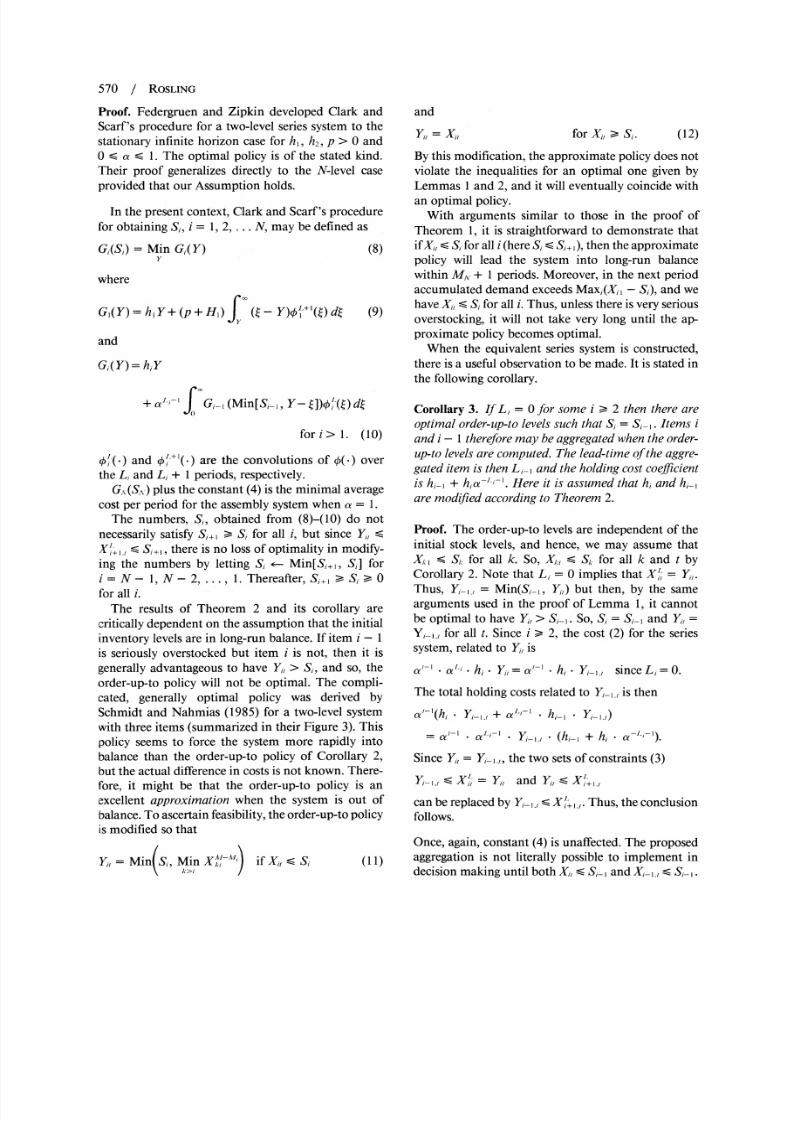
CD,7 Z4=2 z 33usoeoutside 4 3 Customersupply ) ~(9----- ,,1 > demands

lead-time2s=4

21

Figure1. An assembly system.

hope that our results shed some light on this more

complicated problem.The remainder of this paper is organized as follows.

In Section 1, the model is presented.In Section 2, thelong-run analysis of the inventory levelsis carriedout,

and in Section 3 the series interpretationis demon-strated. The analysis of these sections relies on the

assumptionthat all echelon

holdingcosts are

positive.The interestingcasewheresome echelon holdingcosts

are nonpositive is handled in Section 4. In Sections 3and 4, suggestionsaregiven for applying approximate

policieswhen the long-runconditions are not satisfiedinitially. In Section 5, extensions and generalizationsin various directions and to systems with setup costsin production are discussed.Therearetwo appendices.

The first presents some alternativebut equivalent cost

assumptions. The second contains proofs that are

omitted from the main text.

1. THE MODEL

There are N items (components, subassemblies atdifferentlevels, the end item). They are denoted i =

1, 2, . .. N. Item 1 is the end item. Each nonend itemhas exactly one successor item so that the productnetwork formsa tree rooted in the end item. The units

are defined so that exactly one unit of each item is

required for the end item. The following parametersdescribe the system:

s(i) = the unique immediateuccessor of item i = I,2, . . . N; for notational convenience we defines(l) = 0;

A(i) = the set of all successors of item i;P(i) = the set of immediate predecessors of item i =

0, 1, . .. a N;

B(i) = the set of all predecessorsof item i;1,= numberof periods (lead-time)for assembly (or

delivery) of item i.

Everything occurs at the beginning of periods andin the following order. First, outstanding orders forpurchaseand assemblyarriveand new orderingdeci-

sions aremade. Then, old backlogsareexpeditedand,thereafter,customerdemands occur for the end prod-uct. Finally, but still at the beginning of the period,costsare incurred forbacklogand leftover nventories.Holdingcosts arechargedwhen items are in stock butalso when they are in assembly into their successoritem. The following variables areused:

= demands in period t for the end item;demands of different periods are iden-tically and independently distributed,f 0;

/(*), 4(.) = density and distributionfunction for (,;X= E(Q,), he expected value of (,, X> 0;

Xi,= echelon inventory position of item i inperiod t before ordering decisions aremade (= inventory on hand includingallunits already assembledinto otheritems,+ units in assemblyor on order backlogof the end item);

Yi,= echelon inventory position of item i afterproduction decisions are made, Yi,> Xi,;X',= echelon inventory on hand of item i

in period t before ordering decisionsare made but after assembles arrive =

Yi,_,,- J-k-,j Jk. (Throughout this paper,it is assumed that a sum, ',, equalszeroif a > b.) Note that XI, > Y,;, f i E P(k)and if 1,=O then X, = YI,.

Although the demand distributions are assumed tobe stationary, this assumption is of little consequencefor the main results of the next sections. The amount

(Y,, - X,,) is orderedfor the purchaseor assembly ofitem i in period t. It arrivesafter 1iperiods. The costof running the system is determinedby the followingparameters:

Hi = unit installation holding cost per period ofitem i;

hi = unit echelon holding cost per period of item i,

hi,=H -ZkEP(i,H,k;



Optimal InventoryPolicies for Assembly Systems / 567

p = unit backloggingcost per periodof the end item;a = period discount factor, 0 < a < 1.

The values of the cost coefficients are restricted

further n Sections 3 and 4 (the Assumption and the

Generalized Assumption, respectively). There is no

explicit proportional cost of production (or purchase).Appendix A demonstrates that such costs as well as

several other variations of the cost assumptions

can be handled by modifications of the presentcoefficients.

Holding costs are proportionalto installation stockon hand and in assembly into the succeeding item,i.e., to (X',-,) -(XI,),- ,) for i - 2. Total cost in

period t given , is thus

N

i Hj(X'j,I-XI

+ H, *Max(0,X', - ,)+ p *Max(0,(,X',)A'

- hi (X'j- 1) (p + HI) . Max(O, ,-X',)

since Max(0, a) = a + Max(0, -a) and hi = Hi -

ZEkP(i) H,. This reformulation into echelon holdingcosts is similar to Federgruen and Zipkin and is of

critical importance for the subsequent application of

Clark and Scarf's (1960) computational approach.The linearity of the original holdingcosts is apparentlynecessary for its validity. It still works, however, if a

shortage cost, nonlinear in the amount backlogged, s

added to the costs above (cf. Appendix A3).Recallingthat X,+, - +l = Y,- > , the total

expected (E) cost over the infinite horizon can bewritten as

E aE'-' aE '[h1(Y11 X[11 1])]

a "/(p+ HI) X (- Y, 1,O+ ) d() (1)

where fb+(.) is the convolution of k(.) over (1, + 1)

periods. In (1), the present value of the holding costsincurred for item i in period t + 1i s accounted for in

period t, and similarly,the present value of the costsof backlogging in period t + 1, is accounted for in

period t. Consequently, uncontrollable costs due tohistorical decisions are neglected.

For the sequential developments, it is convenient tobreak out from (1) (and sometimes neglect) the con-stant X - [1,+ 1].When this is done, the problemmaybe statedas findingdecisions Yj,,dependenton systemhistory up to period t, that solve problem P.

Problem P

Min E{ a-' al( 1'* hi. Yi,+ ac'(p+ HI)

(t - Y,)k/'+(Q)t)} + constant (2)

such that

x, < Y1i Xl;, for all k E P(i) and all i, t (3)

where

iS=I-Ik

and

Xj,-=Yi,_,-41-l

*= an optimal solution to problem P.

In the case wherea = 1, the average cost per periodis minimized instead of the total discountedcost. Theaveragecost is constructed by multiplying(2) with thediscountrate (1 - a)/a whereaftera -> 1. The lastconstant in (2) (and its average cost analog) equals

A'

-Ehi. X. (i +1)a"i/(1- a) if a <1

N

- hi * X(li+ 1) if a = 1. (4)

2. THE LONG-RUNINVENTORYPOSITION

We need the followingadditionalnotation.

M= total lead-time for item i and all its successors;M,, = 0 and M, i; + XkE() i, for i =

1 2, ... N.

Thus, M, = 11.The items are supposedto be indexed so that

M, a M, for all i and

k, Li a 0 for i = 1,2, ... N.

X = echelon inventory position of item i in periodt orderedLi periodsago or earlier

I -l

- that- E iL=.

Note thatX~',--Yj,if L,= O.



568 / ROSLING

To further clarify the meaning of Xi,, if Z,j, =

order for item i placedj periods ago (i.e., in

period t - j) then

l -I

X', = x', + E j>.j=1.,

- echelon inventory position of item i in periodt ordered M,-, = s periods ago or earlier =

Y,- s _,k= s = 0, 1, .. . , Mi. Note that

it i

it Xk' fork E B(i) [by (3)]

Xi,1'-8 Yi, for,= M,

iAt-8= Xj, forA = M,-I

t= it for, = M_

t= i' for =Mi).

For a given value of ,u both X-'"- and XA'-",k > ibound what is available of the end product within ,utime periods. Thus, they are equally close to the end

item (and the customers), so to speak.Our intended series interpretation requiresthat the

inventory position of the assembly system be in a

certainstate called long-run balance.

Definition (Long-Run Balance)

The assembly system (its inventory position) is in

long-run balance in period t if and only if for i =

1, 2...,5N- I

XA,' X$~ for -0, 1, ..., AMi 1. (5)

Thus, in long-run balance the inventory positions

equallyclose to the end item increasewith i, i.e., withtotal lead-time.

We will demonstrate that optimal policies (among

others) eventually lead the system into long-run bal-

ance and then keep it there. To do this, we restrict hevalues of the cost coefflcients as follows.

Assumption

(i) hi>0 forall iA'

(ii) E - atlu) 0. For the averagecost case (a = 1), it states that all echelon holdingcosts as well as the penaltycost arepositive.Discount-ing in ii is intuitivelydue to the fact thatholding costsarechargedfor item i immediatelyafterassembly, i.e.,

MAl)periods ahead of the earliest possible period in

which it might be sold to a customer (as part of theend product).

Lemma 1. If theAssumptionholds, then or any opti-mal policy for all i and t

Y*= XI ifXi, Min XA,"ik>i

Xi, -, Y* Mi'nX,' if Xi, Min X,-. (6)k;>i k>ij

The proof is in Appendix B. The intuitive messageof

Lemma 1 is illuminating. Since X'-Yi is an upperbound on what possiblycan be made availableof theend product within M, periods of time, then it servesno purpose to produce item i < k in excess of Xk'i.

Such a policy incurs only additional holding costs tothe contrary and, therefore, cannot be optimal. (Itactually suffices to take the minimum of Lemma 1over

Ik> i, k 4 B(I)/Msj) < Mi}. This is so since

X11,-'"i X,,'l/i for all kby definition if I E B(k).)

Lemma 2. If the Assumptionholds thenfor any opti-mal policy, for all i and t

Y* >- Min(O, Min X, i). (7)

An optimalpolicy thus satisfies (on a first-come first-served basis) all customer demands within at most

M, + 1periods of time.

Lemma 2 is proved under more general assump-tions in Appendix B. The assertion is similar to thewell known propertyof the single-itemproblem that

Y* > 0. The only difference is that in the presentcontext there is no reason to produce item i in excessof Xk'jj1',k > i, as noted in Lemma 1. The laststatement of Lemma 2 is similar to the obvious factthat no demand can be backlogged for more thanI+ 1periodsin the single-item model when the order-up-to level is nonnegative.

Theorem 1 (Realization of Long-Run Balance). Anypolicy that satisfies the inequalitiesof Lemmas 1 and2 willeventually ead thesystem into long-runbalanceand keep it there. This will happen no later than MN

+ 1periods aftertheperiodwhen accumulateddemandexceedsMax, Xi,.

Proof. Consider any item i < N. Suppose that periodq(i) is the firstperiod in which there is production ofitem i. By Lemma 1 Y,, S X'i+,,,,and since

,A+ I=Y - < A 1 (- ~t(

v -llit/I I _= x l< j+ l. izt - Aj+ l

(1+ l



OptimalInventoryPolicies for Assembly Systems / 569

also Yi,+I < X'+I+. Repeating this argumentshows thatY,, < Xj'+ for all t - q(i). Moreover, for0 S , M, and t = q(i) + M, -

,-,

- Yiq

Xr

,-,vl. _v _Val-p

< Xfi+iI - > - l

Thus, (5) of the Definition holds for i for all t > q +

M,, and we are done if q(i) < ti _ s + MN - M, + 1for all i, where s is the period when accumulateddemand exceeds Maxi Xi,. This is demonstrated byan inductive argument. Assume that Y,,,3-X'_,+1 i,and q(i) < t, forall i > k. Consideritem k and supposethat y,;,,< X,k=,72 tr This must hold if q(k)> tk since

X- +, < 0. Now

X-1 =-; s+1 ,<k

Ik-I lIk-I

< - Yi, ilk

for all i > k. Since X/,k <0, Lemma 2 implies produc-tion of k with YkIk

-

-= f (,, and consequently,q < tl,. Thus, these inequalities hold for all i > k - 1.The inductive assumption holds for N since tA =

s + 1, X,1,+, < 0 and so, by Lemma 2, YN.+ >- 0.Thus the assumption holds for all i. The assertionfollowsbecauseaccumulateddemand must eventually

exceed any bound as X> 0.

Note that all optimal policies realize long-run bal-ance if the Assumption holds.

The expected time periods until accumulated de-mand exceeds Maxi Xi, is greaterthan Maxi Xi,/ X,but for largevalues of MaxiXi, this is a fairlyaccurateestimate.In a well run system,one expectsXi, to equalthe expected demand over the total lead-time, MA,plus some safety stock. One should, of course, expectsuch a system to be in long-runbalancebut even if itis not, then it can hardly take more than 3(MN+ 1)time periods, say, until it is. Still, the bound of the

theorem is presumablynot very sharp.The modest requirements on a policy to lead the

system into long-run balance can be relaxed furtheras noted in the following corollary. Its proof is con-tained basically in the proof of Theorem 1 and isthereforeomitted.

Corollary 1. Theorem 1 still holds if Mink;>i2'k1 isreplacedbyX , in the inequality of Lemma 1.

In so far as there exist real-life assemblysystems thatliterally satisfy the presentmodel, it would be surpris-ing to find them out of long-run balance.

3. THE EQUIVALENT ERIES SYSTEM

The series interpretationrelies on the assumption thatthe assembly system is in long-run balance from thevery first period. The interpretationof the definitionof long-runbalance when appliedto the initial inven-tory position is investigated at the end of this sectionin Corollary4.

Theorem 2 (The Equivalent Series System). If theAssumptionholds and the assembly system is initiallyin long-run balance, then the optimal policies of theassemblysystemareequivalent o thoseof a pureseriessystem whereitem i immediatelysucceeds item i + 1

and where the lead-time of item i is Li. The costcoefficient p + H1) of the series system is the same asfor the assembly system, but the holding cost coeffi-cients are modifiedso that hi i hi Jai for all i.

Proof. The cost function (2) can be writtenas

Mm (I X

Min El ael-I * ato' i * (hiaeli-Li)Yi1

+ a,'X . (p + HI) ( - Y1}iKv+G()S)}

+ constant.

This verifies the modified cost coefficients. Since thesystem is in long-run balance, and will remain sounder any optimal policy by Theorem 1, X,, =

XiDwI-i\i+ < X jA'lMj+lxA i Xl;, for all

i, t and k E P(i). Because of Lemma 1, (3) thus maybe replacedby X,, Y < Xj',,. ProblemP is restatedas a seriessystem of the asserted kind.

The constant (4) is unaffected by the series re-formulation, and therefore, is calculated in terms ofthe originalcost coefficients.

Corollary 2. Under the assumptions of Theorem 2,thereexist numbersSi, i = 1, 2, . .. N, such that thefollowing order-up-to olicy is optimalfor all i and t

Y*= Min(S, X'? ) if Xi, Si

Y*l = Xi, if Xi,>.s S.

Thenumbers,S,, are convenientlyobtainedby solvingthe series system of Theorem2 by Clark and Scarf's(1960) procedure.



570 / ROSLING

Proof. Federgruenand Zipkin developed Clark and

Scarf's procedurefor a two-level series system to the

stationary infinite horizon case for h,, h2,p > 0 and0 < a < 1. The optimal policy is of the stated kind.Their proof generalizes directly to the N-level case

provided that our Assumption holds.

In the present context, Clark and Scarf'sprocedure

for obtaining Si, i = 1, 2, ... N, may be defined as

Gi(Si) = Min Gi(Y) (8)y

where

GI(Y)= h Y+ (p + HI) (Q Y)0i'`(t) dt (9)

and

Gi(Y)= hiY

+ 'i-l'ri' , (Min[Si-1, Y- p)kL() dt

for i > 1. (1O)

k'(J) and 0 +1(-) are the convolutions of 0(-) overthe Li and Li + 1 periods, respectively.

G,\ S, ) plus the constant (4) is the minimal averagecost per period for the assembly system when a = 1.

The numbers, Si, obtained from (8)-(10) do not

necessarily satisfy Si+, > Si for all i, but since Yi, <

Si+,, there is no loss of optimality in modify-

ing the numbers by letting Si -- Min[Si+,, S] fori = N- 1, N- 2, ..., 1. Thereafter,SI+ S, > 0for all i.

The results of Theorem 2 and its corollary are

critically dependent on the assumptionthat the initial

inventorylevels are in long-runbalance. If item i - 1

is seriously overstocked but item i is not, then it is

generally advantageousto have Yi,> Si, and so, the

order-up-to policy will not be optimal. The compli-cated, generally optimal policy was derived bySchmidt and Nahmias (1985) for a two-level systemwith three items (summarizedin their Figure 3). This

policy seems to force the system more rapidly into

balance than the order-up-to policy of Corollary 2,but the actual differencein costs is not known. There-

fore, it might be that the order-up-to policy is an

excellent approximation when the system is out of

balance.To ascertain easibility,the order-up-topolicyis modified so that

Yi,= Min(Si, MinmI-A') if Xi, S Si (11)

and

Yil = Xi, forX,I>, S,. (12)

By this modification, the approximate policy does notviolate the inequalities for an optimal one given by

Lemmas 1 and 2, and it will eventually coincide withan optimal policy.

With arguments similar to those in the proof of

Theorem 1, it is straightforward o demonstrate thatifXi,< Sifor all i (hereSi Si,+,), hen the approximatepolicy will lead the system into long-run balancewithin MA,+ 1 periods. Moreover, in the next periodaccumulated demand exceeds Max1(X, - Si), and wehaveX1, Si forall i. Thus, unless there is veryserious

overstocking,it will not take very long until the ap-proximate policy becomes optimal.

When the equivalent series system is constructed,

there is a useful observationto be made. It is statedin

the following corollary.

Corollary3. If Li = 0 for some i > 2 then there are

optimal order-up-to evels such that Si = Si-,. Items iand i - 1thereforemay be aggregatedwhen the order-

up-to levels are computed.The lead-timeof the aggre-gated item is thenLi-, and the holdingcost coefficientis hi-, + hia-'-i'. Here it is assumed that hi and hi-are modifiedaccordingto Theorem2.

Proof. The order-up-to levels are independent of theinitial stock levels, and hence, we may assume that

Xl,;?

SI,for all k. So, X,, < S, for all k and t by

Corollary2. Note that Li = 0 implies that X' = Yj,.Thus, Y1-,,,= Min(S_, YJ,)but then, by the same

argumentsused in the proof of Lemma 1, it cannotbe optimal to have Yi,> Si-,. So, S, = Si-, and Yi,=

Yi1 , for all t. Since i > 2, the cost (2) for the seriessystem, relatedto Yi, s

atl-I *a'i * hj* Yj,-='-'- hj* Yj_1, since Li=0.

The total holding costs relatedto Yi1, is then

a-(hi, * Yi 1, + aLi- * hi- Yi- ,)

= a -1I al'j-l . * (hi-, + hi*

Since Yi,= Yi,, the two sets of constraints(3)

Yi_,^ = Y,, and Y,, < X'+,I

can be replacedby Y,1 ' Xf,?,. Thus, the conclusionfollows.

Once, again, constant (4) is unaffected. The proposedaggregationis not literally possible to implement indecision makinguntil both Xi, < Si-, andXi,., ? Si-,.



Optimal InventoryPolicies for Assembly Systems / 571

Furtherdiscussion on the importantnotion of long-run balance is required. The Definition is, unfortu-nately, somewhat confusing, especiallywhen appliedto the initial inventory position. Given Xi, it is appar-

ently of no consequence when this quantity was or-

dered.X$-/ simply does not appear n problem P forg< M,(j).One can thus expect that long-runbalance

be defined with referenceonly to X,'I- for ,This is indeed the case and the definition also can besimplifiedas noted in the following corollary.

Corollary4. Theorems 1 and 2 still hold if the defi-nition of long-runbalance is changedso thatX',- for

,u M.(i) - 1 are replaced by artificial constructs

defined recursively for i = 1, 2, ., N by

Xj,'- X '-,uI - , 1, . ..,M.(j). (13)

Requirement(5) can then be simplifiedso that

X I8, < X I8,it i+ 1.1

only for ,t = MA-1,- . ., M,(j+) (14)

and onlyfori=N- 1,N-2, ...,2suchthati #

s(i + 1).

Proof. We first show that the new constructs are

feasible in P, following (3) and the definition of

X,"'- so that Xj, -y : X,'-y+' and X',ju < XAI'-u for

k E P(i). The first inequality follows from the factthat it holds for i = 1, and if it holds for i, then it

holds for i + 1 since if i = s(i + 1) then

-X;2,"i+l _

il=

_A Aj+, - X"-Ij+,

by (13) and if i $ s(i + 1), then by (14) X"27',

(i + 1 ) >: X ,,- s (i + 1 )

XJ1Al"- (i

+01

X"y'1 (i + 1)+' by (13). The conclusion follows sinceX/'4'i XY'- by (13) for ,t < Mx(j+,).The secondinequality follows because i < k and by (13) and (14),X"'-,u , XjM7$or =O, 1,. .M.,M- 1. Thus, the newdefinition implies the old one, and so, Theorem2 stillholds. To demonstrate that Theorem 1 holds, it suf-fices to show that the old definition implies the newone. This is so because (14) follows directlyif MA,(i)MI,(j+,),and if MAi~,) M4(j+,), then (14) still followsbecause by (13), X',- does not increase.

The requirement (14)needsa comment forthe casewhere i $ s(i + 1) but Mi MAl(i?,)thus, Li = 0);(14) should be checked for g = Mi- 1 and Mi butby (13) it holds for Mi - 1. For ,t = Mi, (14) readsY,, < Xi. ,, and so, whether Xi, < XL+, is to be

checked. The conditions of the corollaryare satisfiedfor the ratherinterestingcase where all initial instal-lation stocks on hand and on order are zero exceptpossibly for the end item.

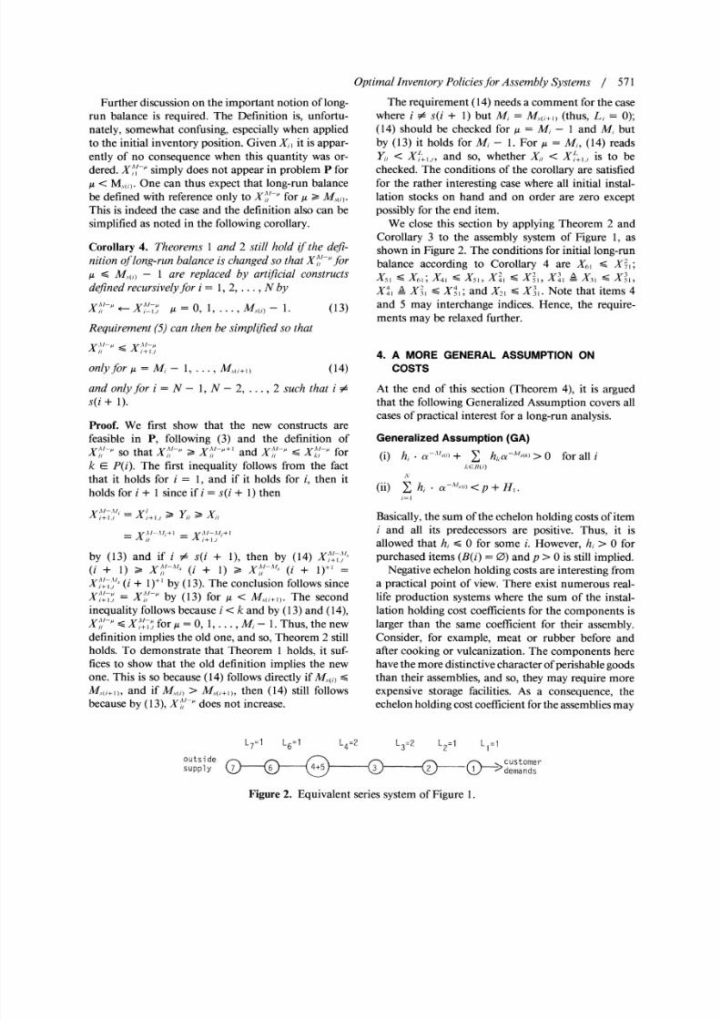
We close this section by applying Theorem 2 andCorollary 3 to the assembly system of Figure 1, asshown in Figure 2. The conditions for initial long-runbalance according to Corollary 4 are X6 7

XS6 Xe t;X4, 'I, X24X X21I, X34 31 X3 I

X41 XX X5; and X2 , X31. Note that items 4and 5 may interchange indices. Hence, the require-ments may be relaxedfurther.

4. A MORE GENERALASSUMPTIONONCOSTS

At the end of this section (Theorem 4), it is arguedthat the following GeneralizedAssumption covers allcases of practical nterest for a long-runanalysis.

Generalized Assumption (GA)

(i) hi . a "Ju) + E hkaj-l'(k))> 0 for all i(kc)(i)

(i) hij ae-Zu) 0 forpurchased tems (B(i) = 0) and p > 0 is. still implied.

Negative echelon holdingcosts are interesting froma practicalpoint of view. There exist numerous real-life production systems where the sum of the instal-lation holding cost coefficients for the components islarger than the same coefficient for their assembly.Consider, for example, meat or rubber before andaftercooking or vulcanization.The components herehavethe moredistinctivecharacterof perishablegoodsthan their assemblies, and so, they may require more

expensive storage facilities. As a consequence, theechelonholding cost coefficient forthe assembliesmay

L7-1 L6=1 L4=2 L3=2 L2=1 L.-=I

outs ide custosupply 7 6 4 +5 2 D >deman

Figure2. Equivalentseriessystem of Figure 1.



572 / ROSLING

be negative. Below (Theorem 3) we present a proce-dure that eliminates all items for which hi ? 0 byaggregating hem into other items.

Lemma 3. Suppose that the GeneralizedAssumption

holds. If hi-

Oor some i, then thereexists an optimalpolicy for which

Y* = Min X', for all t.AGP(i)

A formal proof is found in Appendix B. When hi < 0

there is no cost of holding stocks, and so, as much as

possible is acquiredof item i.For an important special case, the minimum of

Lemma 3 is eventually attained by n E P(i) where nis the immediate predecessor of i's with the smallestlead-time. This is a crucial simplification and the keyto our procedure. Its demonstration requires the fol-

lowing Lemma.

Lemma 4. Lemma 2 holds under the GeneralizedAssumption.

The proof of Lemma 4 is found in Appendix B.

Lemma 5. Supposehi < 0 and h, > O or all k E P(i).If the GeneralizedAssumptionholds, then there existsan optimal policy for whicheventually

Iv (,,

for ,u=0, 1, ...,M,k, k,qeP(i), k<q

x$j,'-'J Xi,7 for , = 0, 1, ..., M,

n is such that Min,; = i,n.k EP(i)

Thus,specifically,Y* - XI.

Proof. Since the proof is similar to earlier ones, wejust give an outline. The availabilityof item k E P(i)affects the availabilityof other items only throughtheavailabilityof item i. Attention therefore can be re-stricted o the subsystemconsistingof i U P(i). It thenfollows by argumentssimilarto those of the proof ofLemma 1 that any optimal policy for the assembly

system is such that for all k E P(i) and all t

Yk*,X, - ifX;, a,;,; ak,= Min Xl,-k/eIN(i)

1>1;

X,;,< Y, ak, ifX,;,< ak,.

Thus, as soon as there is some production of item k,

then Y*, s ak, thereafter,and some periods later it

must be that X"', < XZ'- for all At and I > k,I E P(i). Since X > 0, accumulated demand will

eventually exceed any bound, and so, by Lemma 4,there will be production of all items. Thus, the firstset of inequalities will eventually be satisfied.The lastset of equalities then follows from Lemma 3.

Theorem 3 (Elimination of i for which hi - 0).Consider thefollowing aggregationprocedure:Pick ifor whichhi < 0 and h, > O or all k E P(i); n E P(i)is such that l,,= Mink(,;,) lk Item i is aggregated intoitem n (i.e., eliminated) and thefollowing data modi-fications are carried out.

h,l --hi,* a- + hi, 1,, -- ,, + 1,,s(n) -- s(i)

and P(n) {- JP(i) - n} U P(n)

h, hk -* /, and 1,.-, - l, for kE P(i), k# n.

Theprocedureends whenno such i can befound. Then

D = {i/i has been eliminated}and C = {i/i remains}.

If the GeneralizedAssumption holds then

(i) repeatedapplication of the aggregationprocedureresults in a smaller assembly system that satisfiestheAssumption;

(ii) if Si, i E C, are the reorder evels that eventuallybecome optimal for the aggregated system (byCorollary2) then thefollowing policy for the orig-inal system eventuallyalso becomes optimal

Yi,= Min(Si,X2,j') ifX,, S, | foriE C

Yil=Xi, ifXt>S, k=MinjlEC/l>i}

Yi,= X">'i for i E D, n is the item into which i was

aggregated.

Proof. (i) If item i is aggregated nto item n, then i ofthe GeneralizedAssumptionapparently still holds forthe aggregatedsystem (with item i excluded). Theprocedurecan be repeateduntil hi> 0 for all (remain-ing) i, or it is impossible to find i with hi < 0 such thath, > O or all k E P(i). In the first case, we are doneand in the second case, there must exist i (in theaggregatedsystem) for which hi < 0 and P(i) = 0.

Pick such an i. For the original system the GA impliesthat hi > 0 if P(i) = 0, and so, some items must beaggregated nto i. Since P(i) = 0 after aggregation,these items must have been aggregatedwith all theirpredecessors. Thus, there exists k such that after re-peated application of the cost modification rule, themodified cost coefficient of i is (expressed in theoriginalcoefficients)

hk + E hj a -( v'W_)-M(k)) > 0 by GA(i).je13(k)




This is a contradiction, and so, the assertionfollows.

(ii) If i and n are picked accordingto the procedure,then there is eventually an optimal solution such that

Y* = XI, by Lemma 5. Thus, aggregationof i into n

becomes optimal and we only demonstrate that the

data modifications do not interfere with optimality.By aggregation

/+/,-I

yi.1+1'='

Yli.

-

=l

and so, the parts of (2) concerning i and n (neglectingconstants) are

a a+/n-1 / * hi - Y,,, + > '-h' * Y,

- > t-l a'I'+l(hi h,, a-1j)Y,1,p=1

This verifies the modified cost coefficient for n and

the modified lead-time partly.The lead-time also ap-

pears,however,in (3) fors(i), butXI, of the aggregatedsystem is identical to X', in the original one because1,, -- 1i+ 1,,.Since s(n) -- s(i), the constraint (3) is left

intact. The modification of h, follows from the mod-ification of Ik because a/k * hk - Y,, = a k'1, * hk -

a'- * YA,,.The modification of l,k affects the feasible

set through (3). In terms of the original variables,

Y,l, X',$U forl=

1,;-1,, replaces Y,,

-

X', in (3).Since Yi,, = - s, the new inequality

implies the old one, but by the firstpartof Lemma 5,this does not interferewith optimalityin the long run.

Thus, the inclusion of {P(i) - n} in P(n) is verified

and the data modificationsdo not interferewith long-run optimality. Repeat this argument for every itemthat is aggregated nto another one. From the above

result i, Theorem 1and Corollary2, the assertion then

follows.

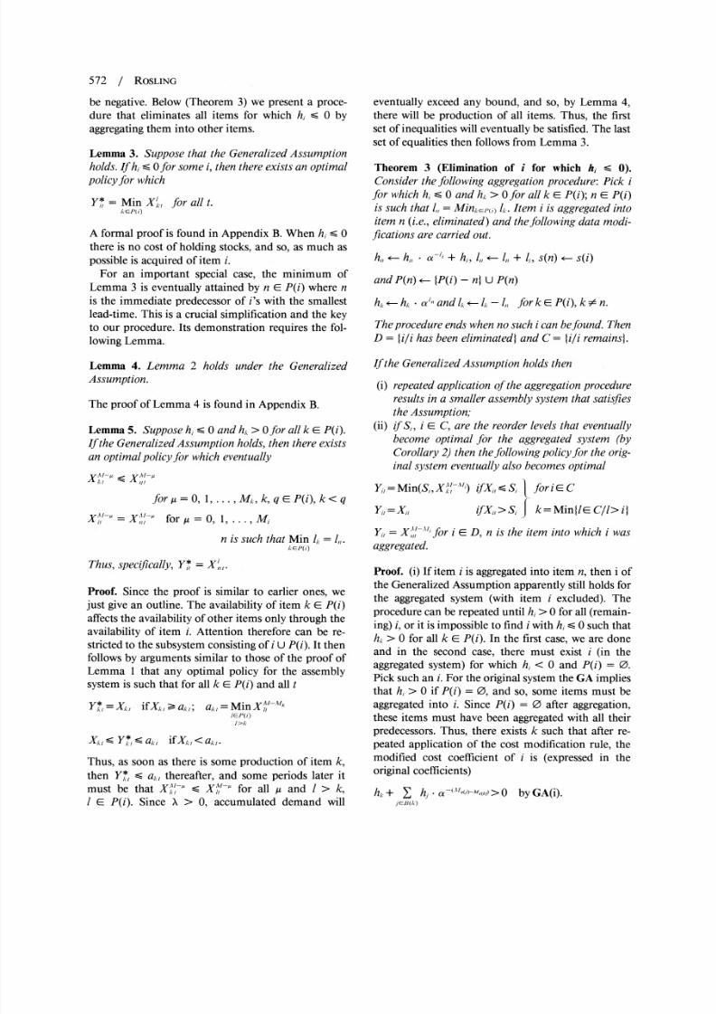
In Figure 3, Theorem 4 is applied to the assembly

system of Figure 1. The policy of Theorem 4 (ii) is

optimal from the firstperiodif the inventory positionof the aggregated ystemis initiallyin long-runbalanceand if, moreover, for i E D, X-,'y = X$"-ufor y =

0, 1, . . ., M- 1. The latter condition is quite strictand we, therefore,proposean approximatepolicy thatis applicable whether or not these requirements are

fulfilled.For those items that remain after aggregation,we

suggestthe policy (1 )-(12) of the last section wherethe minimum is taken over the items of the originalsystem. For items that have been aggregatedawayandfor which hi - 0, we suggestthe policy of Lemma 3.We are then left with those items that have been

aggregatedaway and for which originally hi > 0.Apparently,some other items must have been aggre-

gated into item i before this item was aggregatedaway(since then hi < 0). Consider these other items. Sinceaggregationalways is into a predecessorthey mustform a subtreeof the assembly network. Let I be theroot of the subtree. Aggregation in this subtree)beganwith I and hence h, < 0. We suggest the policy

Yi,= Min X"'-"'i (15)

where Q= Ik> i /k E B(l)}. This policy is an attempt

to ascertainas largea productionas possibleof item I

and simultaneously to take into account that pro-duction of item i in excess of X'-"i, k > i, k E B(l),is useless for this purpose. We expect the suggestedpolicy eventually to coincide with an optimal one,althoughwe have no proof to present.

The question remains whether the GeneralizedAssumption covers all cases of practicalinterest for along-runanalysis.

k7=l Z6-66=1

The aggregated

(D7~ ~ 34+ 1 >system

2=

5i} =4

L7=1 L6=1 L5=4 L2=1 L1=1

X______(i) _____> The equivalent

7u3+4+6

A o 2f 1m>

series system

Figure3. Application f Theorem3 to the assembly ystemof Figure1 (h, < 0 andh4 acK2+ h3 < 0).



574 / ROSLING

Theorem 4 (Practical Necessity of the GeneralizedAssumption).

(i) If hi * a -8s) + ZkEB(i) h,; a (k) < Ofor some i,then the minimal cost ofproblem P is unboundedbelow.

(ii) If i of the Generalized Assumption holdswith semistrict inequality for all items andhi* a- ('m+ XkEB(i) h,k a AI"(k) = 0 for some i

then there is an optimal policy for whichX', isunboundedabovefor all t > MA- M.(i)+ 1.

(iii) If i of the GeneralizedAssumption holds but iidoes not, then there exists an optimal policy forwhich accumulated production is bounded by

Maxk,X,, -Xi, for all i.

The proof of Theorem 4 is in Appendix B.

Casei of the theorem can, of course, only appear npractice as a consequence of incorrectly specifiedmodel data. When these errorshave been rectified weare left with case ii. Here item i is apparentlya free

good, and so, as much as necessaryis acquired of i

and its predecessors.It might take some time beforethis quantityarrivesbut thereafter tem i will never bein shortsupply, and so, item i and all its predecessorscan be neglected in a long-run analysis. We are leftwith case iii of the theorem. Here, the system is notworthoperating n the long run,and so, this case lacksinterest(althoughiii does not formallystate that pro-duction eventually ceases, this is an obvious conjec-

ture). Only systems for which the GeneralizedAssumption holds are left. Thus, all cases of possibleinterestfor a long-runanalysisare covered.

5. EXTENSIONS

Most real-lifeassembly systems are disturbed in oneway or the other by stochastic yields and lead-times.Long-run balance is then attained at most temporarilyand the seriesanalogy does not hold. Still it might bereasonable o model such systems as if yields and lead-times weredeterministic and applythe seriesinterpre-

tation to calculate reasonable order-up-tolevels. Anapproximatepolicy then can be devised, as proposedin Section 3 by (1 )-(12) and in Section 4, Theorem3 for cases that do not satisfythe long-runconditionsinitially.

Frequently,real-lifedemands aremodeled with sea-sonal variations. The series analogy directly carriesover to such nonstationarydemand distributions butthen the order-up-to evels Si are replaced by Si,. The

series interpretationgenerallycannot be expected tocarry over when holding costs or production costs arenonstationary. If it is temporarily advantageous toproduce item i, then it might be optimal to raise itsinventory level above X1+,, and so, the series analogy

breaksdown.It is generallynot possible to apply the seriesanalogy

to systems with setup costs in production. This isobvious when the setup cost of item i is much largerthan for i + 1. Item i is generallyproduced in muchlargerbatches than i + 1, and so, just afterproduction

of item i, one generally expects that Y* > X'?,,contradicting the seriesanalogy. However, there maybe special cases where the seriesanalogymay work asa good approximation.We have in mind cases wherelot sizes increase with i (i.e., with total lead-time) insuch a way that the expected reorder nterval for itemi + 1 is an integer multiple of the same interval for

item i (e.g., a power of two-policy). If item i is aboutto be produced but item i + 1 is not, then X', isgenerally much larger than Xi,, and so, even after

production, Y* < XJ?, as required. If, on the otherhand, i + 1 is about to be produced, then item i issoon to be produced andwe expectthatX' ,,is greaterbut ratherclose to Xi,. If production of item i alwaysis postponed until the production of i + 1 arrives in

Li+,periods,then the seriesanalogywill hold. Presum-ably this postponement generallyincursonly a minordeviation from optimal costs. However, if demandrecently has been high, there can be a profit from

producing a lot of item i immediately, just to makeuseful the excess few units of item i + 1,X?+, -XIas soon as possible. Thus, we make an approximationin addition to the strong assumption about lot sizes

being related to total lead-times. These assumptionsaresimilarto those used by de Bodt and Graveswhenattemptingto extend their series model to a two-levelassemblysystem.

APPENDIXA: VARIATIONSOF THE COSTASSUMPTIONS

1. Sales Prices and Proportional Costs ofProduction

7r= unit sales price of the end product, paid at deliv-ery;

Cj= unit cost of assembly (or purchase) for item iincurredafterassembly (at delivery).

ci is the additional cost of productionof item i so thatthe cost of its predecessor components are not



OptimalInventoryPoliciesfor AssemblySystems / 575

included. Maximizing net profit, the analogy of (1) is

E{ Ea`(r -a"X + -YX1 tI()~

- (- Y, )b`() d]

A'

- E Ci a'i(Yi, -Xi,)i=1

The expected revenues of period t are due to the

expected demand of period t plus expectedbackorderscarried over from period t - 1 minus expected back-orders left at the end of period t.

Using the relation E(X,,) = Y,_- X and adjustingfor constant terms associated with A, (16) can berewrittenas

-Ea1I'* [h, +(l 1-o)c1J

-~~~~~ oa e(i,-li . I])A[i+ ]

1]))

+[p+(l -at)r+HJ]*o/

*f H - Y -Y' 0")dd}

+ constant. (17)

(17) is apparentlyequivalent to (1). To see what costmodifications are actually carried out, write the back-loggingcoefficient as

i=l ~~~i=l

Recalling that Hl = X,= hi, the modifications are

N

E + - a)(ir - - a)c

i-l

and (18)

hj hi +1I-O-)ca.

Thus, revenues as well as production costs may beneglected and problem P applied.

2. Reduced HoldingCosts DuringAssembly

Q,j= reductionof the echelon holding cost per periodof item j during assembly of item i j, A, hiif i<jand Al,- 0 if i =j.

It seems fairlynatural that holding costs are differentwhen items areon the assembly line and in the storageroom. Not only arereductionspermitted by the abovedefinition but as j = i is allowed, the possibility ofholding costs incurred from the moment of orderingis also accounted for.

The reducedechelon holding costs duringassemblyare handled indirectly by a reduction in the produc-tion costs. The present value (at delivery)of the costreductionduringassemblyof one unit of item i is

E A,j(a' + a2 + *-- + a1i)*jE=_B(i)uji)

As demonstrated in the previous section, a propor-tional cost of production, c,, may be eliminated if(1 - a) - ci is added to the echelon holding costcoefficient. Thus

hi <hi- i A-,(a-li1).

With this modification of hi, the model is equivalentto problem P. Note that when a = 1 there is, in fact,no modification (except for the constant of (17)).

3. A Fill-RateTypeShortage Cost

b = unit cost of backlogging[$/unit].

While p with dimension [$/unit x time] is naturallyassociated with stockout constraints of the type aver-age outstanding backordersper period, b is naturallyassociated with a fill rate type constraint, averagenumber of demands per period not satisfieddirectlyfrom stock on hand.

Since stock on hand first is used to satisfy oldbacklogs,the discounted expected cost for new back-logs in period t + 1 is

a1* b * a(f (Q Yj,O+'+() dt

Q - Y, O'(Q)d#) (19)

where 0'(.) is the convolution of O(*)over 1, periods.When adding(19) to the other costs of (1), a modi-

fication of ii of the GeneralizedAssumption is neces-saryfor our results to carryover. To see the nature of



576 / ROSLING

the modification rewrite i of the GeneralizedAssump-tion as

N hi(a - 1 p

E 1-a i- (20)

The left-hand side is the present value (at the deliveryof the end product) of all holding costs for the com-ponents incurred during production. The right-hand

side is the present value of the unit cost of backloggingover the entire infinite horizon. To take b into

account, (20) is modified so that

A hi(aAl,') - 1) p (21)

i=l 1 -ea 1 - a

As long as p > 0 or a < 1, ii should thus be modifiedto

N

ihi a-'u) < p + H, + (1 - a)b. (22)

However, if p = 0 and a = 1 then (22) is not correct.

The limit is taken directlyfrom (21) so that

N

hi M(i < b. (23)

Replacementof ii of the GeneralizedAssumptionwith

(22) and (23) is sufficient for all our results to carryover except for the order-up-to policy of Corollary 1and Theorem 3. Since (19) is not convex in Y,,thereis no guarantee that (1) will remain unimodal in Yi,after the addition of (19). Thus, when X'+,, < Si it

might be that an optimal policy requires Y* < X,'because of a local minimum. Neglectingthis anomalyis, presumably, an acceptable approximation.

APPENDIX B: OMITTEDPROOFS

Proof of Lemma 1

If an optimal policy, Y* (with states X), violatesthe assertion, then for some i and t (and some out-

comes of demands) Y* > Xi, and Y* > XZ,'-M'i

Min,k>i ,-'i. Then define an alternative policy Y(with statesX) which deviates from Y* by

Fit= Max(X,,, X,,'-xli) andY,(k), = Min(Y(/), Ak'q)

for all k EI{i}IU A(i), q =t + Mi- I,(k-,. (24)

Policy Y postpones production of item i in period t,one period ahead. If required for feasibility (by (3)),some production is also postponed a period for itemk E A(i) in period t + M, - M,;.Note that Y satisfiesthe assertion for i and that it is feasible for P. Since

YF, Yi*, Y,V, Y*, and hk > 0 for all k and s, the

holding costs of (2) are lower for Y than for Y*.Consider the backloggingcosts of (2). They are the

same for Yas for Y* if Y, = Y*, where r = t + M, -

M,. This will be demonstrated. Pick j, k, n E A(i)such that j E P(l), j = s(k) and k = s(n). Let u =

r-4 and w = u-1,;. Then by (24)

Xj -pj,. = YJ*,-yj,,

= Max(O,YJ,,-X/_) - Max(O,Xj,-X, i).

Similarly, X$'-' -1 = Y* y_Max(O,Xkl - X;,7') and so,

X//

= iMlax(O,j.-X j,. + Max(O,X,, -X*?, ))

= Max(O,XJ, X,," 1)since X>j, X,,Al by (3).

Extending this analysis to all items of A(i) and when

i is included (note that Yj,= Min(Y*, YF,))we get

X',-X = Max(O,X',-I

Pick m E A(b) such that m E P(1) and consider the

difference

AT -' Xj, = (X/1?/ NJ,) (Xjr. -JAr)

=(X/,), - Xj.) + Max(O,X, - X',jIxI). (25)

Suppose that XII - XI,?,.Since YV, XAf,I,jXAl-A,

Xh>" and so

Xi/' -,lZrjX/

bl- 0

by definition and (3).

Thus, XX,,Xj =X, -Xj. so that Xj, = Xj, and= Y*, by (24). Suppose that XI' > X/?. If

X', XX',, then Y,, = Y* again. Suppose that X, >

X' Then by (25), necessarily, X', > X,". Butthen by (25) (note that X" ',- X',- by definitionand (3))

X I- X + X /- AT = X/0 -All

1)71 Jl 1)1/ Jl Jl 171 1)? 1

6 ,? x)l ={AI1 X7,A[,. < 0

by assumption.

Thus, XI, < X/ and since Y*, - XI, by (3), Y,, =Y,*by (24). Hence, the backloggingcosts are the samefor Yand Y* and so, Yis superior o Y*, contradictingits optimalityand the conclusion follows.

Proof of Lemma 2

TheAssumption implies the GeneralizedAssumption,and so, Lemma 2 follows directlyfrom Lemma 4.The proof of Lemma 4 requires the followingproposition.



OptimalInventoryPoliciesfor Assembly Systems / 577

Proposition

Let I C {1, 2, ..., N} and A = UiE, A(i). If the

GeneralizedAssumptionholds then

i hia",u) hiao1 ) + > hia-','i) h/; a*1Ix(Ak} < 0 by GA(i)ici kEBB(i)

So, the conclusion follows.

Lemma4. If the GeneralizedAssumption holds, then

for any optimal policy

Y* >,-Min O MiXkm for all i and t. (26)kv>i

Such a policy satisfies (on a first-come first-servedbasis) all customer demands within at most MN + 1

periods of time.

Proof. The first assertion is demonstrated by an

inductive argument. Suppose a feasible policy (inter-

preted as a function of demand history only) has been

fixed for all i > n and, given this restriction, optimalvalues, Y,,, have been computed for all i < n - 1 and

t. The inductive hypothesis says there is a solution for

which (26) holds for all i - n - 1 regardless of what

feasible policies were fixed for i > n. This (partial)

optimization is repeated and this time it also includes

i = n and feasible policies are fixed only for i 2 n +

1. By the inductive hypothesis, there is a solution for

which (26) holds for all i < n - 1 and t. By a

contradictive argument, (26) will also hold for i = n.

So, given some fixed policies for i > n, pick an optimal

solution Yj, (with states Xi,), i - n, for which (26)

holds for i < n and where for at least some t, say

t = q,

Ynql Min (O, X '-).k>,,

Note that Y<q<0 so that there are outstanding back-

orders for the end item. Define a new policy Yi,for all

i - n and t. To do this note that by the inductive

hypothesis for i < n, Y1, -XAI,i for t = q + Mn- M

because X>jl' Yn,,, 0 by definition. Then define

An={n U {i< n/Yl, =X$ ,'-fort= q+ M,, M1

and the new policy Yi, with statesXN,)or i < n by

Yi,= YF, for all t if i i A or

if iEA fort<q+Mn-M,

Yi,=

Yi, +e

foriEA andt=q+M,7-M,Yj,= Max(Y1,, Xj,)

foriEA andt>q+M,,-M,. (27)

The new policy is feasiblebecausen > i implies thatM,,> M, by definition. It is assumed that E is small

enough so that if i M A, then Yj-

X '-i for t =

q + M,, M1.The new policy suppliesc more units ofthe end item in period q + M,/. Beforecomputing thecost implications, note that by (3) i M A implies thats(i) 4 A since

v-1

=Av iv,v - r, +

,,1

where I = s(i), r= q + M,, Ml and v = q + MnMi. Consequently, i 4 A implies that 1 4 A for all/ E B(i) and A is similar to the set appearingin theProposition. The difference of e additional units instock for the new policy will prevail until some pro-duction is scheduledby the old one by (27). For somerealization of demands, suppose 6 < Eunits of the enditem areproduced by Yin period q + M,,+ T(possibly,

T = oo).The total gain in costs of backlogging s then

a 23 oea'-I* . (p + HI)/qt+AI,n-/1

= - (p + HI) acI+' (1 -o )/(I - a).

For this production to be feasible there must be pro-duction of item i E A in period q + M,, + T- Mi orearlier.Thus, an upperbound on the additionalhold-ing cost is

v+T- I

6 . >fi fi a'-' a*'i hi

= . a+l.' hi . (1 -iT)/(I - a)

where v = q + M,,- Mi. Thus, there is a net gain for

M,(i) Mi - 1i nd by the Proposition

Ehia-'"ZSu)< p + H

Thus, the newpolicy givesa net gainforallrealizationsof demand and the optimality of the original one iscontradicted.A similar but much simpler argument



578 / ROSLING

shows that the inductive hypothesis holds for n = 1.Thus, the first assertionis demonstrated. The secondone is a directconsequence.

Proof of Theorem 4

(i) Considerthe subsystem {i} U B(i) and supposethat a finite optimal policy exists. Then consideran alternativepolicy that orders one more unitin period 1 of the component, m, with thegreatest total lead-time M11, in period M,,, -

Ml + 1 of the component, 1, with the next tothe greatest total lead-time and so on, so thatone more unit is ordered of item i in period

M,- Mi + 1. This additional unit is held instock forever. The additional cost of this policyis for the first M,,, - Mi periods (capitalizedtoperiodM,,1-M1 + 1)

E h a 'k(1 + a + + aAlk-AXl-) a-Wk-_,d

IkEB(i)

or equivalently

h, * a1k(a-U"I,k-`i) - 1)/(1 - a).k G B (i)

The cost of holding item i foreverfrom period

M.- M1+ 1 on is

hi aia+ fi hkg a'k/ (1 -a).k EB(i) J

So, the total cost increaseis

alj'(h,+ ,kEBsi) hk,; a- '1s(k;)- l'.si)))

1 -a <O

by assumption.

Thus, the conclusion follows.

(ii) As above, except that the final inequality is anequality.

(iii) Consider the final item and suppose that in

periodt, Y*, > X, and accumulatedproduc-tion exceeds Max,<X,, - X,. Consequently,accumulated production of item i exceeds

Max,kXI, - X,, in period t - (Ml - M) = torearlier.Consideran alternativepolicy Ysuchthat Yj,= Y-*- 6 for all t > (t, or the firstearlierperiod with production > 0) where 6 >Os arbitrarily mall. The cost savingof having6 units less in stock over the entire horizon isat least (capitalizedto t, + L,)

A'

8 hii, ",w( - a).

The increase in penalty costs over the sameperiod is

b(p + H,)/(1 - a).

By assumption, E',,a(-"l(i) >

p + H, and so,the new policy is as good as the old one,verifying the proposition for i = 1. Considernext all i E P(1). If hi > 0, the conclusiondirectly carries over to item i, but if hi < 0,then there is an independent motive for build-ing up stocks of item i. Considerthe subsystem{i} U B(i) and apply the same argument as forthe final item. The same conclusion followsbecause GA(i) holds for i. These argumentscarryover to all i.

ACKNOWLEDGMENT

The advice of an anonymous referee considerablyimproved this paper. The research was supportedby the Swedish National Board for TechnicalDevelopment.

REFERENCES

AXSATER,., ANDP. LUNDELL. 984. In Process-SafetyStocks. In Proceedingsof 23rd Conference n Deci-sionand Control,pp. 839-842. Las Vegas.

BESSLER,. A.,AND

A. F. VEINOTT. 966. Optimal Policyfor a Dynamic Multiechelon Inventory Model.Naval. Res. Logist.Quart.13, 355-389.

CARLSON, . C., AND C. A. YANO. 1986. Safety Stocksin MRP-Systems with Emergency Setups for Com-ponents. Mgmt. Sci. 32, 403-412.

CLARK,A. J., AND H. SCARF.1960. Optimal Policies fora Multiechelon Inventory Problem. Mgmt. Sci. 6,475-490.

CLARK, A. J., AND H. SCARF. 1962. Approximate Solu-tions to a Simple Multi-Echelon Inventory Problem.In Studies in AppliedProbabilityandManagementScience, pp. 88-110. K. J. Arrow, S. Karlin andH. Scarf (eds.). Stanford University Press, Stanford,

CalifDE BODT,M. A., AND S. C. GRAVES. 1985.Continuous-Review Policies for a Multi-Echelon InventoryProblem with Stochastic Demand. Mgmt. Sci. 31,

1286-1299.FEDERGRUEN, A., AND P. ZIPKIN. 1984. Computational

Issues in an Infinite-Horizon, Multi-Echelon Inven-tory Model. Opns.Res. 32, 818-836.

FUKUDA, Y. 1961. Optimal Disposal Policies. NavalRes.Logist. Quart.8, 221-227.

HOCHSTADTER, D. 1970. An Approximation of the Cost




Function for a Multi-Echelon Inventory Model.Mgmt. Sci. 16, 716-727.

KARMARKAR, U. S. 1981. The Multiperiod,Multiloca-tion InventoryProblem.Opns.Res. 29, 215-228.

KARMARKAR, U. S. 1987. The Multilocation,Multiper-iod Inventory Problem: Bounds and Approxima-tions. Mgmt. Sci. 33, 86-94.

ROSLING, K. 1977.A Generalization f Clarkand Scarf'sApproach o Multi-EchelonInventoryControl.InThree Essays on Batch Productionand Optimiza-

tion, pp. 20- 111. Linkopings Tryckeri AB.Linkoping,Sweden.

ROSLING,K. 1989. Bounding Procedure or Clark andScarf's Serial Multi-Echelon Inventory Model.

Working Paper, Departmentof ManagementandEconomics, Linkoping Institute of Technology.S-581 83 Linkoping,Sweden.

SCHMIDT,C. P., AND S. NAHMIAS. 1985. OptimalPolicyfor a Two-Stage Assembly System Under Random

Demand. Opns.Res. 33, 1130-1145.

Documents

Assembly System