arX

iv:q

uant

-ph/

0604

094v

1 1

2 A

pr 2

006

Decoy state quantum key distribution with two-way classical

post-processing

Xiongfeng Ma,1, ∗ Chi-Hang Fred Fung,1, † Frederic Dupuis,2, ‡

Kai Chen,1 Kiyoshi Tamaki,3, § and Hoi-Kwong Lo1, ¶

1Center for Quantum Information and Quantum Control,

Department of Physics and Department of Electrical & Computer Engineering,

University of Toronto, Toronto, Ontario, Canada

2Departement IRO, Universite de Montreal, Montreal, H3C 3J7 Canada

3NTT Basic Research Laboratories, NTT corporation,

3-1,Morinosato Wakamiya Atsugi-Shi, Kanagawa, 243-0198, JAPAN

Abstract

Decoy states have recently been proposed as a useful method for substantially improving the

performance of quantum key distribution protocols when a coherent state source is used. Previously,

data post-processing schemes based on one-way classical communications were considered for use

with decoy states. In this paper, we develop two data post-processing schemes for the decoy-state

method using two-way classical communications. Our numerical simulation (using parameters

from a specific QKD experiment as an example) results show that our scheme is able to extend

the maximal secure distance from 142km (using only one-way classical communications with decoy

states) to 181km. The second scheme is able to achieve a 10% greater key generation rate in the

whole regime of distances.

PACS numbers: 03.67.Dd, 03.67.Hk

∗Electronic address: xima@physics.utoronto.ca†Electronic address: cffung@comm.utoronto.ca‡Electronic address: dupuisf@iro.umontreal.ca§Electronic address: tamaki@will.brl.ntt.co.jp¶Electronic address: hklo@comm.utoronto.ca

1

I. INTRODUCTION

Quantum key distribution (QKD) allows two users, commonly called Alice (sender) and

Bob (receiver), to communicate in absolute security in the presence of an eavesdropper, Eve.

Unlike classical cryptography, the security of QKD is based on the fundamental principles

of quantum mechanics, rather than unproven computational assumptions.

The best-known QKD protocol—the BB84 scheme—was published in 1984 [1]. In BB84,

Alice sends Bob a sequence of single photons each of which is randomly prepared in one of

two conjugate bases. Bob measures each photon randomly in one of two conjugate bases.

Alice and Bob then publicly compare the bases and keep only those results (bits) for which

they have used the same bases. They randomly test a subset of those bits and determine

the quantum bit error rate (QBER). If the QBER is larger than some prescribed value,

they abort the protocol. Otherwise, they proceed to the classical data post-processing

(which consists of error correction and privacy amplification) and generate a secure key.

The security of BB84 has been rigorously proven in a number of papers [2, 3, 4], see also [5].

The security proof in [4] shows that the BB84 protocol can be successively reduced from

a entanglement distillation protocol (EDP). This idea is relevant to this paper since our data

post-processing schemes are based on EDPs. We remark that EDPs were first discussed in

[6], that its relevance to the security of QKD was emphasized in [7], and that this connection

was established rigorously in [3]. The EDPs proposed earlier use local operations and one-

way classical communications (1-LOCC). Later, Gottesman and Lo provided security proofs

of standard quantum key distribution schemes by using a EDP with local operations and

two-way classical communications (2-LOCC) [8]. They showed that BB84 using 2-LOCC

can tolerate a higher bit error rate than 1-LOCC (see also [9]). On the other hand, Gerd,

Vollbrecht and Verstraete also proposed another EDP that uses a 2-LOCC based recurrence

scheme [10]. Although their scheme was originally proposed as an EDP, we will use it here in

a QKD to increase the key generation rate. [It should be noted that the EDP approach is only

one of the several approaches to security proofs of QKD. Other useful approaches to security

proof can be based on, for example, communication complexity [11], quantum memory

[12, 13], or direct information-theoretic argument [15].] Recently, it has been demonstrated

[14] rigorously that one can generate a long secure key even when the amount of distillable

entanglement in a quantum state is arbitrarily small. In other words, secure key generation

2

is strictly weaker than entanglement distillation. Recently, the universal composability of

quantum key distribution has been proven in [16].

In summary, QKD is secure in theory. Much of the interest in QKD is due to its po-

tential in near-term real-life applications. Indeed, commercial optical-fiber-based quantum

cryptographic products are already on the market [17].

Meanwhile, experimentalists have done many QKD experiments, such as [18] and [19, 20].

The key issue in QKD experiments is whether they are really secure. Standard security

proofs are often based on perfect devices, such as perfect single photon sources. All devices

are imperfect in real implementations, such as imperfect single photon sources and highly

lossy channels. It is thus important to study the security of QKD with imperfect devices.

Substantial progress has been made in the subject [21, 22, 23].

Unfortunately, with the method in GLLP [22], QKD can only be proven to be secure

at very limited key generation rates and distances. It came as a big surprise that a simple

solution to the problem — the decoy state method — actually exists. The decoy method was

first discovered by Hwang [24], and made rigorous by our group [25, 26], and also [27, 28]. In

addition, our group demonstrated the first experimental implementation of a QKD protocol

using one decoy state [29].

The usefulness of decoy state protocols over non-decoy-state protocols have previously

been demonstrated [25, 26], within the context of 1-LOCCs, for an imperfect source. Since

2-LOCCs are known to be superior to 1-LOCCs for a perfect source [8, 9, 10], it would be

interesting to study the usefulness of decoy state protocols with 2-LOCCs, for an imperfect

source. This is the main goal of this paper. Indeed, as we will show, decoy state protocols

with 2-LOCCs are superior to decoy state protocols with only 1-LOCCs in realistic situations.

Specifically, in this paper, we develop two data post-processing schemes for the decoy method

of [25, 26] by applying two 2-LOCC EDPs, Gottesman-Lo EDP [8] and the recurrence scheme

[10]. Both methods are superior to the random hashing 1-LOCC EDP (for the rest of the

paper, we will simply call it as the 1-LOCC EDP) in two different aspects in the case of

ideal devices; the Gottesman-Lo EDP was shown to be able to achieve a higher tolerable

bit error rate, while the recurrence method was shown to be able to achieve a higher key

generation rate. We will show in this paper that the same conclusion holds in the case of

imperfect devices. In particular, depending on the distance in a QKD experiment, one can

use our Gottesman-Lo EDP based data post-processing scheme in the long distance region

3

or our recurrence based data post-processing scheme in the short distance region to increase

the key generation rate.

We note that a recent and independent analysis of combining B steps with GLLP and

decoy states is given in [30]. Their data post-processing scheme is the same as our first

scheme, which is aimed at increasing the maximal secure distance. On the other hand, in

this paper, we also propose the second scheme, which is aimed at increasing the key rate at

short distances.

The organization of this paper is as follows: We first review entanglement distillation in

Section II and some existing techniques for realistic QKD in Section III. We then investigate

the tolerable error rates, the upper bounds of secure distance and key generation rate in

Section IV. Sections V and VI contain the main results of the paper. Specifically, we

develop two data post-processing schemes, one with the B steps from Gottesman and Lo [8]

(see Section V), and the other with recurrence (see Section VI). Our simulation (based on

the GYS experiment [19]) shows that with B steps from Gottesman-Lo EDP, the maximal

secure distance can be extended to 180km compared with 140km with 1-LOCC, and the

key generation rate increased by more than 10% in the whole regime of distances. With our

QKD model, we also consider statistical fluctuations on the estimated parameters when the

data has finite length (see Section VII). The result shows that the B step can extend the

maximal secure distance and the recurrence can raise the key generation rate. Although,

in this paper, we focus on the BB84 protocol, our schemes can be applied to other QKD

protocols as well.

II. REVIEW OF ENTANGLEMENT DISTILLATION

In this section, we review Shor-Preskill’s security proof of QKD and two EDPs based

on 2-LOCC (Gottesman-Lo EDP and recurrence EDP) assuming that ideal single-photon

sources are used. In Sections V and VI, we generalize these two schemes for realistic setups.

The idea of the Shor-Preskill [4] security proof of QKD is to apply an EDP to show that

the leaked information about the final key is negligible. Here we will explain how to analyze

the security of EDP-based QKD.

4

In the EDP-based QKD protocol, Alice creates n+m pairs of qubits, each in the state

|ψ〉 = 1√2(|00〉+ |11〉),

the eigenstate with eigenvalue 1 of the two commuting operators X⊗

X and Z⊗

Z, where

X =

0 1

1 0

, Z =

1 0

0 −1

are the Pauli operators. Then she sends half of each pair to Bob. Alice and Bob sacrifice m

randomly selected pairs to test the error rates in the X and Z bases by measuring X⊗

X

and Z⊗

Z. If the error rates are too high, they abort the protocol. Otherwise, they conduct

the EDP, extracting k high-fidelity pairs from the n noisy pairs. Finally, Alice and Bob both

measure Z on each of these pairs, producing a k-bit shared random key about which Eve has

negligible information. The protocol is secure because the EDP removes Eve’s entanglement

with the pairs, leaving her negligible knowledge about the outcome of the measurements by

Alice and Bob.

In the EDP, after the qubits’ transmission, Alice and Bob will share the state with density

matrix,

ρ =

q00 × × ×× q10 × ×× × q11 ×× × × q01

, (1)

normalized with q00 + q10 + q11 + q01 = 1. Here ×’s denote arbitrary numbers, all of which

are not necessary the same, and the density matrix is in the Bell basis:

|ψ00〉 =1√2(|00〉+ |11〉)

|ψ10〉 =1√2(|01〉+ |10〉)

|ψ11〉 =1√2(|01〉 − |10〉)

|ψ01〉 =1√2(|00〉 − |11〉).

Since all EDPs we consider in this paper do not make use of the off-diagonal elements in

Eq. (1) to extract entanglement, it is sufficient to characterize the density matrix by only

the diagonal elements (q00, q10, q11, q01). In fact, any shared state can always be transformed

5

into a diagonal form by local operations and classical communications [33]. The density

matrix is now a classical mixture of the Bell states ψij with probabilities qij . Therefore, the

bit and phase error rates are given by

δb = q10 + q11

δp = q11 + q01.(2)

A QKD protocol based on a Calderbank-Shor-Steane (CSS) [31] EDP can be reduced to

a “prepare-and-measure” protocol (BB84) [4]. That is to say, CSS codes correct bit errors

and phase errors separately, which respectively turn out to be the bit error correction and

privacy amplification in the context of QKD [4]. Thus the key rate of this 1-LOCC based

data post-processing scheme is given by [4, 32],

RCSS = q [1−H2(δb)−H2(δp)] , (3)

where q depends on the implementation (1/2 for the BB84 protocol, because half the time

Alice and Bob bases are not compatible, and if we use the efficient BB84 protocol [47], we

can have q ≈ 1.), δb and δp are the bit flip error rate and the phase flip error rate, and H2(x)

is the binary entropy function,

H2(x) = −x log2(x)− (1− x) log2(1− x).

In summary, there are two main parts of EDP, bit flip error correction (for error cor-

rection) and phase flip error correction (for privacy amplification). These two steps can be

understood as follows. First Alice and Bob apply error correction, after which they share

the same key strings but Eve may still keep some information about the key. Alice and

Bob then perform the privacy amplification to expunge Eve’s information from the key. We

remark that the key generation rate achieved by Eq. (3) requires only 1-LOCC.

A. Gottesman-Lo EDP

Gottesman and Lo [8] introduced an EDP based on 2-LOCC for use with QKD and

showed the it can tolerate a higher bit error rate than 1-LOCC based EDP’s. B and P steps

are two primitives in the Gottesman-Lo EDP, and the EDP consists of executing a sequence

of B and/or P steps, followed by random hashing. The random hashing part is a one-way

6

EDP. The main objective for extra B and P steps is reduce the bit and/or phase error rates

of qubits so that the random hashing can work to extract secure keys. This is the reason

why the Gottesman-Lo EDP is able to tolerate a higher initial bit error rate than one-way

EDPs. The definitions of B and P steps are as follows.

Definition of B step [8]: (Figure 1) After randomly permuting all the EPR pairs, Alice

and Bob perform a bilateral XOR (BXOR) between pairs of EPR pairs and measure the

target qubits in Z basis. This effectively measures the operator Z⊗

Z for each of Alice

and Bob, and detects the presence of a single bit flip error. If Alice and Bob’s measurement

outcomes disagree, they discard the remaining EPR pair, otherwise, they keep the control

qubit.

FIG. 1: Alice and Bob choose two half EPR pairs and input the quantum circuit as shown above.

They discard both control and target qubits if they disagree on the outcome of measurement on

the target qubits. On the other hand, they keep the control qubits as surviving qubits if their

measurement outcomes agree.

Since the B step only involves the measurement of Z⊗

Z, it can be used in the prepare-

and-measure protocol, BB84. Classically, the B step simply involves random pairing of the

key bits, say x1, x2 on Alice’s side and y1, y2 on Bob’s side and the computation of the parity

of each pair of bits, x1 ⊕ x2 and y1 ⊕ y2. Both Alice and Bob announce the parities. If their

parities are the same, they keep x1 and y1; otherwise, they discard x1, x2, y1 and y2. We

can see that the B step is very simple to implement in data post-processing.

Suppose Alice and Bob input: a control qubit (qC00, qC10, q

C11, q

C01) and a target qubit

(qT00, qT10, q

T11, q

T01) with bit error rates δCb and δCp and phase error rates δTb and δTp , respec-

tively. After one B step, the survival probability pS is given by,

pS = (qC00 + qC01)(qT00 + qT01) + (qC10 + qC11)(q

T10 + qT11)

= (1− δCb )(1− δTb ) + δCb δTb ,

(4)

7

and the density matrix (q′00, q′10, q

′11, q

′01) of output control qubit is given by

q′00 =qC00q

T00 + qC01q

T01

pS

q′10 =qC10q

T10 + qC11q

T11

pS

q′11 =qC10q

T11 + qC11q

T10

pS

q′01 =qC00q

T01 + qC01q

T00

pS.

(5)

Eqs. (5) can be derived from TABLE II of [33]. The corresponding bit error rate δb and

phase error rate δp can be obtained from Eq. (5) by

δ′b = q′10 + q′11 =δCb δ

Tb

pS

δ′p = q′11 + q′01.

(6)

Definition of P step [8]: Randomly permute all the EPR pairs. Afterwards, group the

EPR pairs into sets of three, and measure X1X2 and X1X3 on each set (for both Alice and

Bob). This can be done (for instance) by performing a Hadamard transform, two bilateral

XORs, measurement of the last two EPR pairs, and a final Hadamard transform. If Alice

and Bob disagree on one measurement, Bob concludes the phase error was probably on one

of the EPR pairs which was measured and does nothing; if both measurements disagree for

Alice and Bob, Bob assumes the phase error was on the surviving EPR pair and corrects it

by performing a Z operation.

Without a quantum computer, Alice and Bob are not able to perform the P steps, so the

EDP cannot depend on the results of P steps. When the P step is implemented classically

in BB84, the phase errors are not detected or corrected (i.e. the phase flip operation Z is

not applied). The P step then will be reduced to: Alice and Bob randomly form trios of

the remaining qubits and compute the parity of each trio, say x1 ⊕ x2 ⊕ x3 by Alice and

y1⊕ y2⊕ y3 by Bob. They now regard those parities as their new bits for further processing.

Since before P steps, Alice and Bob will do random permutation, for simplicity, we assume

the input three qubits have the same density matrix: (q00, q10, q11, q01). After one P step,

8

the density matrix (q′00, q′10, q

′11, q

′01) of the output qubit is given by

q′00 = q300 + 3q200q01 + 3q210(q00 + q01) + 6q00q10q11

q′10 = q310 + 3q210q11 + 3q200(q10 + q11) + 6q00q10q01

q′11 = q311 + 3q10q211 + 3q201(q10 + q11) + 6q00q11q01

q′01 = q301 + 3q00q201 + 3q211(q00 + q01) + 6q10q11q01,

(7)

which is given in Appendix C of [8]. So the bit error rate and phase error rate will given by

δ′b = q′10 + q′11 = 3δb(1− δb)2 + δ3b

δ′p = q′11 + q′01 = 3δ2p(1− δp) + δ3p .(8)

Here we emphasize that the B and P steps are important elements of the Gottesman-Lo

EDP. After B and P steps, the Gottesman-Lo EDP will be the same as the regular 1-LOCC

EDP.

B. Recurrence EDP scheme

Here we review another two-way EDP, the recurrence scheme [10]. Similar to the B step

in Gotttesman-Lo EDP, the recurrence scheme reduces the bit error rate of the EPR pairs

before passing them to the 1-LOCC based random hashing for the distillation of maximally-

entangled EPR pairs. However, there are two main differences between these two EDP

schemes. The first is how the bit error syndrome of a target EPR pair in a bilateral XOR

operation is learned. In Gotttesman-Lo EDP, Alice and Bob simply measure the target EPR

pair in the Z basis and compare their results to learn the bit error syndrome (see Figure 1).

In the recurrence scheme, Alice and Bob group the bit error syndromes of all target EPR

pairs together and learn all the syndromes using random hashing. The second difference

is that the recurrence scheme requires some extra maximally-entangled EPR pairs to begin

with for learning the bit error syndromes, whereas no such extra pairs are required in the

Gotttesman-Lo EDP. We note that the recurrence methods have been studied in various

papers, such as [7, 48, 49, 50].

The steps for the recurrence protocol are as follows:

1. Alice and Bob perform BXOR using two noisy EPR pairs as the sources and one

perfect maximally-entangled EPR pair as the target.

9

2. They do random hashing on the target EPR pairs to learn the parities of noisy EPR

pairs. Note that only a portion of the target EPR pairs have to be measured in order

to learn all the parities. This is different from the B step approach.

3. They do error correction and privacy amplification separately for even-parity EPR

pairs and odd-parity EPR pairs.

The key generation rate using the recurrence EDP with a single-photon source is given

by

R = q

[

−1

2H2(pS)−

1

2pSH2(

δCb δTb

pS) +K

]

(9)

where q is defined similarly as in Eq.(3), pS (given in Eq. (A2)) is the probability of getting

even parity, and δCb (δTb ) is the bit error rate of the control (target) EPR pair. Here, the first

term in the bracket corresponds to the extra perfect EPR pairs borrowed, the second term

corresponds to error correction, and the third term K (given in Eq.(A12)) corresponds to

privacy amplification. In Appendix A, we review the recurrence EDP in detail and develop

the key rate formula.

III. REVIEW OF REALISTIC QKD

In this section, we set up a model for realistic QKD, and review the idea of GLLP and

decoy-state QKD.

A. Realistic QKD setup

In this section, we present a commonly used fiber-based QKD system model. All later

simulations of QKD are based on this model. In order to describe a real-world QKD system,

we need to model the source, transmission and detection. Here we consider a widely used

QKD setup model with polarization coding [34], see also [26].

Source: The laser source used in the QKD experiment can be modeled as a weak coherent

state. Assuming that the phase of each pulse is totally randomized, the photon number of

each pulse follows a Poisson distribution with a parameter µ as its expected photon number

set by Alice. Thus, the density matrix of the state emitted by Alice is given by

ρA =∞∑

i=0

µi

i!e−µ |i〉〈i|, (10)

10

where |0〉〈0| is vacuum state and |i〉〈i| is the density matrix of the i-photon state for i =

1, 2 · · · . The states with only one photon (i = 1) are normally called single photon states.

The states with more than one photon (i ≥ 2), on the other hand, are called multi photon

states. Here, we assume Eve receives all the pulses sent by Alice. Eve performs some

arbitrary operations and sends either a vacuum or a qubit to Bob. This is the squash

operation introduced in GLLP [22]. Consequently, we denote the qubits coming from these

three states as vacuum qubits, single photon qubits and multi photon qubits.

A vacuum qubit is a qubit sent by Eve when Alice sent a vacuum state. (In the case

without Eve’s presence, it is some random qubit stemmed from the dark counts of Bob’s

detector or other background contributions.) Thus, it does not contribute to the key gener-

ation. Due to photon-number splitting (PNS) attacks [35, 36, 37, 38], multi photon states

are not secure for the BB84 protocol. Here is a key observation of this QKD model: the final

secure key can only be extracted from single photon qubits [52]. Besides BB84, this is true

for most present QKD protocols, such as E91 [39], B92 [40] and the six-state [41] scheme.

One exception is the SARG04 protocol [42], in which two-photon states can also contribute

to the secure key generation rate [43, 44].

Transmission: For optical fiber based QKD systems, the losses in the quantum channel

can be derived from the loss coefficient α measured in dB/km and the length of the fiber l

in km. The overall transmittance is given by

η = ηBob10−αl

10 . (11)

where ηBob denotes for the transmittance in Bob’s side, including the internal transmittance

of optical components and detector efficiency. Here we assume a threshold single photon

detector on Bob’s side. That is to say, we assume that Bob’s detector can tell whether there

is a click or not. However, it cannot tell the actual photon number of the received signal, if

it contains at least one photon.

It is reasonable to assume independence between the behaviors of the i photons in i-

photon states. Therefore the transmittance of i-photon state ηi with respect to a threshold

detector is given by

ηi = 1− (1− η)i (12)

for i = 0, 1, 2, · · · .

11

Yield: Define Yi to be the yield of an i-photon state, i.e., the conditional probability of a

detection event at Bob’s side given that Alice sends out an i-photon state. Note that Y0 is the

background rate which includes detector dark counts and other background contributions

such as the stray light from timing pulses.

The yield of the i-photon states Yi mainly comes from two parts, the background and

the true signal. Assuming that the background counts are independent of the signal photon

detection, then Yi is given by

Yi = Y0 + ηi − Y0ηi

∼= Y0 + ηi.(13)

Here we assume Y0 (typically 10−5) and η (typically 10−3) are small.

The gain of i-photon states Qi is given by

Qi = Yiµi

i!e−µ. (14)

The gain Qi is the product of the probability of Alice sending out an i-photon state (fol-

lows Poisson distribution) and the conditional probability of Alice’s i-photon state (and

background) that will lead to a detection event in Bob’s detector.

Quantum Bit Error Rate (QBER): The error rate of i-photon states ei is given by

ei =e0Y0 + edηi

Yi(15)

where ed is the probability that a photon hit the erroneous detector. ed characterizes the

alignment and stability of the optical system. Experimentally, even at distances as long as

120km, ed is independent of the distance [19]. In what follows, we will also assume that ed

is independent of the transmission distance We will assume that the background is random.

Thus the error rate of the background is e0 = 1

2. Note that Eqs. (12), (13), (14) and (15)

are satisfied for all i = 0, 1, 2, · · · .The overall gain is given by

Qµ =

∞∑

i=0

Yiµi

i!e−µ. (16)

The overall QBER is given by

Eµ =1

Qµ

∞∑

i=0

eiYiµi

i!e−µ. (17)

12

Without Eve, a normal QKD transmission will give

Qµ = Y0 + 1− e−ηµ

EµQµ = e0Y0 + ed(1− e−ηµ).(18)

B. GLLP idea

We review the idea of GLLP’s [22] briefly here. GLLP gives a security proof of BB84

QKD when imperfect devices (such as imperfect single photon sources) are used. There are

two kind of qubits discussed in GLLP, tagged qubits and untagged qubits. Tagged qubits

are those that have their basis information revealed to Eve, i.e. tagged qubits are not secure

for QKD. On the other hand, untagged qubits are secure for QKD. In BB84, qubits coming

from single-photon states are untagged while those from multi-photon states are tagged

because Eve, for instance, can perform PNS attacks [35, 36, 37, 38] to the multi-photon

states to acquire their basis information. The essential idea of GLLP is that Alice and Bob

can apply privacy amplification to tagged and untagged qubits separately. Note that the

idea of tagged state was (perhaps implicitly) introduced by [21].

The data post-processing of GLLP is performed as follows. First, Alice and Bob apply

error correction to all qubits, sacrificing a fraction H2(δ) of the key, which is represented in

the first term of Eq. (19). Secondly, in principle, Alice and Bob can distinguish the tagged

and untagged qubits, so they can apply the privacy amplification on the tagged state and

untagged state separately. One can imagine executing privacy amplification on two different

strings, the qubits stagged and suntagged arising from the tagged qubits and the untagged qubits

respectively. Since the privacy amplification is linear (the private key can be computed by

applying the C2 parity check matrix to the qubit string), the key obtained is the bitwise

XOR

suntagged ⊕ stagged

of keys that could be obtained from the tagged and untagged qubits separately [22]. If

suntagged is private and random, then it doesn’t matter if Eve knows anything about stagged —

the sum will be still private and random. Thus, one only needs to apply privacy amplification

to the untagged bits alone.

We define the residue of data post-processing to be the ratio of the final key length to the

sifted key length (in an asymptotic sense). The residue of this data post-processing scheme

13

is given by

rGLLP = max−f(δ)H2(δ) + Ω[1−H2(δp)], 0 (19)

where δ is the overall quantum bit error rate (QBER), Ω is the fraction of untagged qubits

(Ω = 1−∆, where ∆ is the fraction of tagged qubits defined in GLLP [22]), δp is the phase

error rate of the untagged qubits, f(·) is the error correction efficiency as a function of error

rate [46], normally f(x) ≥ 1 with Shannon limit f(x) = 1, and H2(x) is binary entropy

function.

We can further extend GLLP’s idea to the case of more than two classes of qubits, i.e.

several kinds of qubits with flag g, which generalizes the concept of tagged and untagged

qubits. The procedure of data post-processing is similar, do the overall error correction first

and then apply the privacy amplification to each case. So the privacy amplification part can

be written as∑

g

ΩgH2(δgp) (20)

where one needs to sum over all cases with flag g, Ωg is the probability of the case with flag

g and∑

g Ωg = 1, and δgp is the phase error rate of the state with flag g. At last, the residue

of data post-processing is given by

r = max−f(δ)H2(δ) +∑

g

Ωg[1−H2(δgp)], 0. (21)

Apply the QKD model described in Section IIIA here, δ = Eµ and the key generation

rate is given by

R = q ·Qµ · r, (22)

where Qµ and Eµ is the gain and QBER of the signal state, and q is defined similarly as in

Eq.(3).

C. Decoy states

For BB84, the single photon state is the only source of final secure keys, i.e. the untagged

qubits come from single photon qubits. So the fraction and error rate of untagged qubit are

given by

Ω = Q1/Qµ

δp = e1,(23)

14

where Q1 is given in Eq. (14), e1 is given by Eq. (15), and Qµ is given by Eq. (16). By

substituting Eq. (19), we can rewrite Eq. (22) into

R = q · r ·Qµ

≥ q · −Qµf(Eµ)H2(Eµ) +Q1[1−H2(e1)],(24)

which is given in Eq. (11) of [25].

Qµ and Eµ can be measured directly from experiment. The question is how to estimate

Q1 and e1 accurately? In principle, Eve can perform non-demolition photon number mea-

surement on the qubits and she may change the yields (Yi in Subsection IIIA) of the qubits

depending on the measurement outcomes. That is, the yields of qubits, in general, may

depend on the photon number. Moreover, Eve can adjust the error rates as she wishes.

The key idea of decoy states is that, instead of just using one coherent state for key

transmission, Alice and Bob choose some decoy states with different expected photon num-

bers (µ in Subsection IIIA) to test the channel transmittance and error rate. We emphasize

here that decoy states have exactly the same properties other than average photon numbers,

so that there is no way for Eve to discriminate between the signal states and decoy states

before Alice publicly announce them. Consequently, we have Yi(decoy) = Yi(signal) and

ei(decoy) = ei(signal).

Specifically, the overall gain and the overall QBER in Eq. (16) and Eq. (17) can be

estimated for a fixed µ in the experiment by Alice and Bob. By changing µ over many

values, a set of linear equations in the form of Eq. (16) and Eq. (17) with unknowns Yi’s and

ei’s are obtained. Thus, Alice and Bob can easily solve for Yi’s and ei’s from these equations.

For BB84, they are only interested in Y1 and e1. With the decoy state, Alice and Bob can

estimate the yields and error rates of single photon states (Y1 and e1) accurately.

Here we will briefly review the results of decoy state protocols. Details can be seen in

[25] and [26]. In the asymptotic decoy states case [25], we assume that infinite decoy states

are employed by Alice and Bob, so they can solve the infinite number of linear equations

in the form of Eq. (16) and Eq. (17) to get all values of Yi and ei accurately. In the

simulation, we will simply take the value of Eq. (13) and Eq. (15) directly.

In the practical case, Alice and Bob only need to use two decoy states, a vacuum and

15

weak decoy state. Then they can bound Y1 and e1 by (Eq. (34) and Eq. (37) in [26])

Y1 ≥µ

µν − ν2(Qνe

ν −Qµeµ ν

2

µ2− µ2 − ν2

µ2Y0)

e1 ≤EνQνe

ν − e0Y0Y1ν

,

(25)

where ν is the expected photon number of weak decoy state. We remark that when ν → 0,

Eqs.(25) will asymptotically approach Eq. (13) and Eq. (15).

IV. BOUNDS

In QKD experiments, we are interested in maximizing three quantities – the tolerable

error rates, the key generation rate and the maximal secure distance. In this section, we

will give out these three bounds due to QKD setup model discussed in Subsection IIIA.

A. Bounds of error rates

Here, we will consider the bounds of error rates (bit error rate δb and phase error rate

δp), assuming a laser source that emits a fixed number of photons in each pulse (e.g. a basis-

dependent single-photon source). The upper bounds can be derived by considering some

simple attacks (such as intercept-resend attack) and determining the QBER caused by these

attacks. The lower bounds can be determined by the unconditionally security proof assuming

that Eve is performing arbitrary attack allowed by the law of quantum mechanics and Alice

and Bob employ some special data post-processing schemes (such as Gottesman-Lo EDP

described in Subsection IIA). One lower bound, obtained by considering Gottesman-Lo

EDP, is 18.9% [8]. For BB84, an upper bound, obtained by considering an intercept-resend

attack, is 25%.

Here, we consider the lower bound in a general setting that the error rates are charac-

terized by (δb, δp). In general, the bit error rate δb can be measured by error testing, but

the phase error rate δp cannot be directly observed from the QKD experiment. In order to

guarantee the security, Alice and Bob have to bound δp with the knowledge of δb. For BB84

with an ideal single-photon source, due to the symmetry between the X and Z bases, one

can show that the bit error rate and the phase error rate are the same, i.e.

δb = δp. (26)

16

In general, for other protocols or with non-ideal sources (including coherent sources), the

bit and phase error rates are different. For example, even for BB84, when a basis-dependent

source is used, Eq. (26) may not hold. In this case, according to the idea of [32], we can

show that δb and δp have the relation of

F ≤√

(1− δb)(1− δp) +√

δbδp, (27)

where F is the fidelity between the two states sent by Alice corresponding to the two bases

and is the single parameter that characterizes the basis dependency of the source. Thus,

Alice and Bob can upper bound δp (denoted as δup ) with this inequality given δb. Clearly,

when δp = δb, the inequality will be always satisfied, i.e., δp = δb is a particular solution of

Eq. (27). Therefore, in general we have δup ≥ δp. In the following, we use δp to denote the

upper bound δup for simplicity.

Given a QKD protocol and a laser source, Alice and Bob can estimate the phase error

rate δp from the bit error rate δb according to the protocol and the source. We investigate

the highest error rates that a data post-processing scheme can tolerate. Fig. 2 shows the

tolerable error rates of the Gottesman-Lo EDP compared to the 1-LOCC EDP scheme,

illustrating the superior performance of the Gottesman-Lo EDP over the 1-LOCC EDP.

The boundaries of error rates are found by searching through the regime of

δb ≤ δp

δb + δp < 1/2(28)

such that positive key rates are obtained. The reason we are interested in the region specified

the second inequality in Eq. (28) is as follows: We can assume that the error rates δb and δp

are less than 1/2, otherwise Alice and Bob can flip the qubits. Also, if δb + δp ≥ 1/2, then

all the diagonal elements of the density matrix in Eq. (1) Alice and Bob share are no greater

than 1/2 (by setting q11 = 0). Thus, the diagonalized density matrix is separable [33] and

the Gottesman-Lo EDP cannot distill any pure EPR pairs.

The input to the Gottesman-Lo EDP is (q00, q10, q11, q01) with q00 + q10 + q11 + q01 = 1,

see in Subsection IIA. But Alice and Bob only know δb = q10 + q11 and δp = q11 + q01 from

their error test. There is one free parameter q11. In Appendix C of [8], the authors have

proved that q11 = 0 is the worst case when δb = δp. Following that proof, we can show that

q11 = 0 is the worst case when the condition of Eq. (28) is satisfied. That is, given (δb, δp), if

17

we check the input (1− δb − δp, δb, 0, δp) for Gottesman-Lo EDP and get a positive key rate,

then we can safely claim that Gottesman-Lo EDP can tolerate the error rates of (δb, δp).

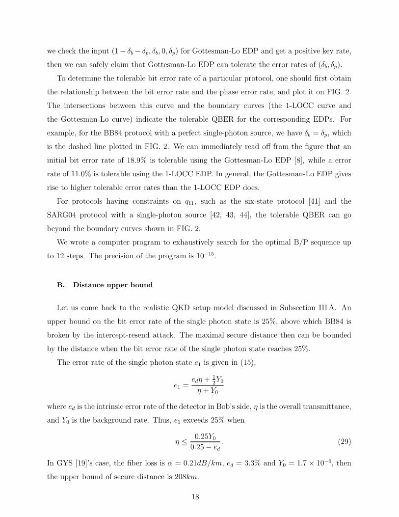
To determine the tolerable bit error rate of a particular protocol, one should first obtain

the relationship between the bit error rate and the phase error rate, and plot it on FIG. 2.

The intersections between this curve and the boundary curves (the 1-LOCC curve and

the Gottesman-Lo curve) indicate the tolerable QBER for the corresponding EDPs. For

example, for the BB84 protocol with a perfect single-photon source, we have δb = δp, which

is the dashed line plotted in FIG. 2. We can immediately read off from the figure that an

initial bit error rate of 18.9% is tolerable using the Gottesman-Lo EDP [8], while a error

rate of 11.0% is tolerable using the 1-LOCC EDP. In general, the Gottesman-Lo EDP gives

rise to higher tolerable error rates than the 1-LOCC EDP does.

For protocols having constraints on q11, such as the six-state protocol [41] and the

SARG04 protocol with a single-photon source [42, 43, 44], the tolerable QBER can go

beyond the boundary curves shown in FIG. 2.

We wrote a computer program to exhaustively search for the optimal B/P sequence up

to 12 steps. The precision of the program is 10−15.

B. Distance upper bound

Let us come back to the realistic QKD setup model discussed in Subsection IIIA. An

upper bound on the bit error rate of the single photon state is 25%, above which BB84 is

broken by the intercept-resend attack. The maximal secure distance then can be bounded

by the distance when the bit error rate of the single photon state reaches 25%.

The error rate of the single photon state e1 is given in (15),

e1 =edη +

1

2Y0

η + Y0

where ed is the intrinsic error rate of the detector in Bob’s side, η is the overall transmittance,

and Y0 is the background rate. Thus, e1 exceeds 25% when

η ≤ 0.25Y00.25− ed

. (29)

In GYS [19]’s case, the fiber loss is α = 0.21dB/km, ed = 3.3% and Y0 = 1.7 × 10−6, then

the upper bound of secure distance is 208km.

18

0 0.05 0.1 0.15 0.2 0.25 0.3 0.35 0.4 0.45 0.5 0

0.05

0.1

0.15

0.2

0.25

0.3

0.35

0.4

0.45

0.5

Phase flip error rate δp

Bit

flip

erro

r ra

te δ

b

18.9%

11.0%

Gottesman−Lo 1−LOCC

BB84

FIG. 2: shows the secure regions in terms of error rates for 1-LOCC EDP and Gottesman-Lo EDP.

The regions under solid lines are proven to be secure due to 1-LOCC EDP, and Gottesman-Lo EDP

schemes (for the region under the solid line and dashed line), respectively. For 1-LOCC EDP, we

use Eq. (3). For Gottesman-Lo EDP, we use Eqs. (5) and (7). In Gottesman-Lo EDP, we optimize

the B/P sequence up to 12 steps.

C. Key generation rate upper bound

According to our model, the final secure key can only be derived from single photon

qubits. To derive the upper bound of key generation rate, we assume that Alice and Bob

can distinguish the single photon qubits from other qubits (say, vacuum and multi photon

qubits). So they can perform the classical data post-processing only on to the single photon

qubits. One upper bound of key generation rate is given by the mutual information between

Alice and Bob [45],

RU = Q1[1−H2(e1)], (30)

where Q1 is the yields of single photon states and e1 is the error rate of single photon states.

Note that the above two upper bounds, Eqs. (29) and (30), assume that a) Alice and Bob

cannot distinguish background counts and true signal counts and b) secure key can only be

19

extracted from the single photon states. Also, these two bounds are general upper bounds

regardless of the technique used for combating the effect of imperfect devices such as the

decoy-state technique.

V. DECOY + GLLP + GOTTESMAN-LO EDP

In this section, we propose a new 2-LOCC based data post-processing protocol with a

form of a sequence of B steps, followed by error correction and privacy amplification, as

discussed in Subsection IIA. This new scheme is a generalization of the Gottesman-Lo

scheme to the case of imperfect devices. The reasons why we skip P steps here are as

follows. First, from the simulation in Subsection IVA, we found that P steps are not as

useful as B steps. Secondly, only considering B steps can simplify the procedure of the data

post-processing scheme.

The procedure of this data post-processing is as follows.

1. Alice and Bob perform a sequence of B steps to the sifted keys (corresponding to rB

in Eq. (31)).

2. They calculate the variables (such as QBER, untagged qubits ratio) after the B steps.

3. They perform overall error correction (corresponding to the first term in Eq. (31)).

4. They perform privacy amplification (corresponding to the second term in Eq. (31)).

In the following, we will discuss how to calculate the residue of this data post-processing

scheme.

In the decoy protocol, there are three kind of qubits: vacuum, single photon and multi

photon qubits, described in Section IIIA. We emphasize again here that the final secure key

can only be distilled from untagged qubits (single photon qubits).

Since either of the two inputs of a B step has three possibilities, the outcomes of a B

step then have nine possibilities. Only the case that both inputs are untagged qubits has

positive contribution to the final secure key and all other privacy amplification terms in

Eq. (21) will be 0. That is, at the end of some B steps and bit error correction, privacy

amplification can be only applied to the remaining qubits that come from the case where

both inputs are untagged qubits. In other words, an output qubit after a subsequence of B

20

steps is “untagged” iff a) it passes all B steps and b) it is generated from the case where

all initial input qubits are single photon qubits. Therefore, the residue ratio of data post

processing can be expressed, according to Eq. (21), as

r = maxrB[−f(δ)H2(δ) + Ω(1−H2(δuntaggedp ))], 0 (31)

where δ is the overall QBER, rB is overall survival residue, Ω is the fraction of untagged

states in the final survival states and δuntaggedp is the phase error rate of the untagged states,

after a sequence of B steps. In the following, we will show how these variables change with

performing B steps.

An arbitrary B step: B step is an important two-way primitive that we will use in this

paper. Let us consider how the various quantities (fraction of untagged states Ω, QBER of

overall surviving states δ, bit error rate δuntagged and phase error rates δp of the untagged

states) are transformed under one step in a B step sequence.

Before a B step, the fraction of untagged states is Ω, the overall QBER is δ, the bit error

rate of the untagged states is δuntagged, and the phase error rate of the untagged states is δp.

According to Eq. (4) the overall survival probability pS and the survival probability of the

untagged states puntaggedS after one B step are given by

pS = [δ2 + (1− δ)2]

puntaggedS = [δ2untagged + (1− δuntagged)2].

(32)

Then the residue after one B step is given by,

rB =1

2pS (33)

The factor 1

2in Eq. (33) due to the fact that Alice and Bob only keep one qubit from a

survival pair. Then, after a B step the fraction of untagged states Ω′ is given by

Ω′ =Ω2 · puntaggedS

pS. (34)

Overall QBER: the change of overall QBER δ′ is given by

δ′ =δ2

δ2 + (1− δ)2. (35)

Untagged states: before the first round of B step, the initial density matrix of untagged

state is (1−2e1+ q11, e1− q11, q11, e1− q11), where e1 is the error rate of single photon states.

21

From Appendix C of [8], we know that q11 = 0 is the worst case for B steps. Thus we can

conservatively choose (1 − 2e1, e1, 0, e1) as the initial input density matrix. If only B steps

are performed, q11 = 0 will always be satisfied, according to Eq. (5). So the input untagged

qubits for any round of B step has the form of

(q00, q10, q11, q01) = (1− δuntagged − δp, δuntagged, 0, δp). (36)

The bit error rate of untagged state δ′untagged only depends on the input δuntagged,

δ′untagged =δ2untagged

δ2untagged + (1− δuntagged)2. (37)

According to Eqs. (5), (6) and (36), the phase error rate of untagged states is

δ′p = q′11 + q′01

=2q10q11 + 2q00q01

(q10 + q11)2 + (q00 + q01)2

=2δp · (1− δuntagged − δp)

δ2untagged + (1− δuntagged)2.

(38)

Eqs. (32)-(38) are valid for a general B step. Alice and Bob can perform a sequence

of B steps as described above and then do the error correction and privacy amplification.

Once all the these quantities are obtained, the key generation rate can be calculated from

Eq. (31).

To illustrate the improvement made by introducing B steps, we numerically calculated

the key generation rate assuming the parameters in the GYS experiment [19]. Note that

the overall QBER δ in Eq. (31) never exceeds 10%. The value of f(e) = 1.22 is the upper

bound according to [46]. The parameters used for simulation are listed in Table I.

Wavelength [nm] α [dB/km] ηBob ed Y0

1550 0.21 4.5% 3.3% 1.7× 10−6

TABLE I: Data come from GYS [19].

From FIG. 3, we can see that there is a non-trivial extension of maximal secure distance

after introducing B steps. We remark that the key generation rate decoy state protocol

with 1 B step is higher than the one with 1-LOCC from the distance around 132km. The

maximal secure distance using 4 B steps is 181km, which is not far from the upper bound

22

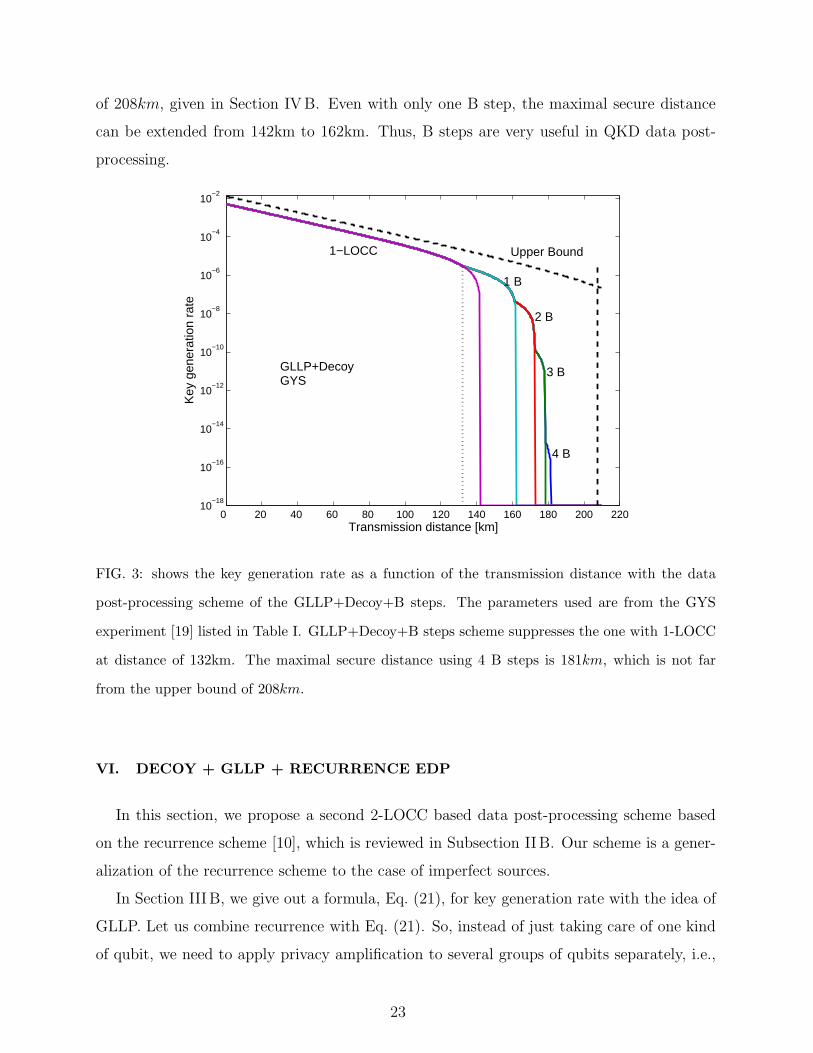
of 208km, given in Section IVB. Even with only one B step, the maximal secure distance

can be extended from 142km to 162km. Thus, B steps are very useful in QKD data post-

processing.

0 20 40 60 80 100 120 140 160 180 200 22010

−18

10−16

10−14

10−12

10−10

10−8

10−6

10−4

10−2

Transmission distance [km]

Key

gen

erat

ion

rate

Upper Bound 1−LOCC

1 B

2 B

3 B

4 B

GLLP+DecoyGYS

FIG. 3: shows the key generation rate as a function of the transmission distance with the data

post-processing scheme of the GLLP+Decoy+B steps. The parameters used are from the GYS

experiment [19] listed in Table I. GLLP+Decoy+B steps scheme suppresses the one with 1-LOCC

at distance of 132km. The maximal secure distance using 4 B steps is 181km, which is not far

from the upper bound of 208km.

VI. DECOY + GLLP + RECURRENCE EDP

In this section, we propose a second 2-LOCC based data post-processing scheme based

on the recurrence scheme [10], which is reviewed in Subsection IIB. Our scheme is a gener-

alization of the recurrence scheme to the case of imperfect sources.

In Section IIIB, we give out a formula, Eq. (21), for key generation rate with the idea of

GLLP. Let us combine recurrence with Eq. (21). So, instead of just taking care of one kind

of qubit, we need to apply privacy amplification to several groups of qubits separately, i.e.,

23

we will have several Ki in Eq. (A6). After the recurrence, the data post-processing residue

rate becomes

r = −1

2f(pS)H2(pS)−

1

2pSf(

δ2

pS)H2(

δ2

pS) +

∑

i

ΩiKi, (39)

where pS is the even parity possibility given in Eq. (A2) with δCb = δTb = δ, δ is the

overall QBER before the recurrence, f(·) is error correction efficiency, Ωi and Ki are the

probability and the residue of the qubit groups with label i after privacy amplification,

respectively. Here, Alice and Bob first check the parity, corresponding to the first term

of Eq. (39). Secondly, they apply overall error correction to the qubits with even parity,

corresponding to the second term of Eq. (39). Thirdly, they measure one of qubits in those

pairs with odd parity to obtain the error syndrome of another qubit. Afterwards, they can

group the surviving qubits into several groups with labels i. Finally, they perform privacy

amplification to each group with label i, corresponding to the last term of Eq. (39).

Consider the decoy state case, Alice and Bob have three kinds of input qubits: vacuum

qubits (V), single photons qubit (S) and multi photon qubits (M). The input parameters for

recurrence are listed in Table II.

Qubit Fraction δb δp q11

V ΩV 1/2 1/2 qV11

S Ω e1 e1 a

M ΩM eM 1/2 qM11

TABLE II: lists the input parameters of three kinds of qubits for recurrence. Following Eq. (14)

and (16), the fractions of each group are given by ΩV = Q0/Qµ, Ω = Q1/Qµ and ΩM = 1−ΩV −Ω.

ΩV /2 + e1Ω+ eMΩM = δ is the overall QBER.

Thus, the outcome of one round of recurrence will have nine cases. Clearly, if neither

input is a single photon qubits, the outcome will have no contribution to the final key. Alice

and Bob need only apply Eq. (A12) to calculate the residues, Ki, for the five cases: V⊗

S,

S⊗

V , S⊗

S, S⊗

M , M⊗

S. The probabilities of occurrence, Ωi, for the five cases are,

respectively, ΩVΩ, ΩΩV , Ω2, ΩΩM , ΩMΩ. Once we know Ki and Ωi, we can then determine

the overall residue, r, using Eq. (39) (details are shown in Appendix B):

r ≥− B + C − Fa (40)

24

where

B =1

2f(pS)H2(pS) +

1

2pSf(

δ2

pS)H2(

δ2

pS)

C =3

4ΩVΩ + Ω2(1− e1 + e21) +

1

2ΩΩM (2− e1 − eM + 2e1eM)

D1 =3

4ΩVΩ +

1

2Ω2(2− e1) +

1

2ΩΩM (2− eM )

D2 =3

4ΩVΩ +

1

2Ω2(1 + e1) +

1

2ΩΩM (eM + 1)

Fa = D1(1− e1)H2(e1 − a

1− e1) +D2e1H2(

a

e1)

(41)

with equality when qV11 = 1/4 and qM11 = eM/2. In order to get a lower bound of key

generation rate R, we maximize Fa over a by using a bisection method as discussed in

Appendix B.

0 20 40 60 80 100 120 140 160 18010

−8

10−7

10−6

10−5

10−4

10−3

10−2

Transmission distance [km]

Key

gen

erat

ion

rate

[per

pul

se]

Recurrence1 B1−LOCC

FIG. 4: Plot of the key generation rate as a function of the transmission distance,

GLLP+Decoy+Recurrence vs. GLLP+Decoy+1-LOCC. Recurrence does have some marginal im-

provement over 1-LOCC for short distances. In particular, the recurrence method increases the

key generation rate by more than 10% in our simulation. The maximal secure distance for each

case is 142.8km (1-LOCC), 149.1km (Recurrence), 163.8km (1B), respectively. Here we consider

the asymptotic Decoy state QKD case with infinitely long signals. The parameters used are from

the GYS experiment [19] listed in Table I.

25

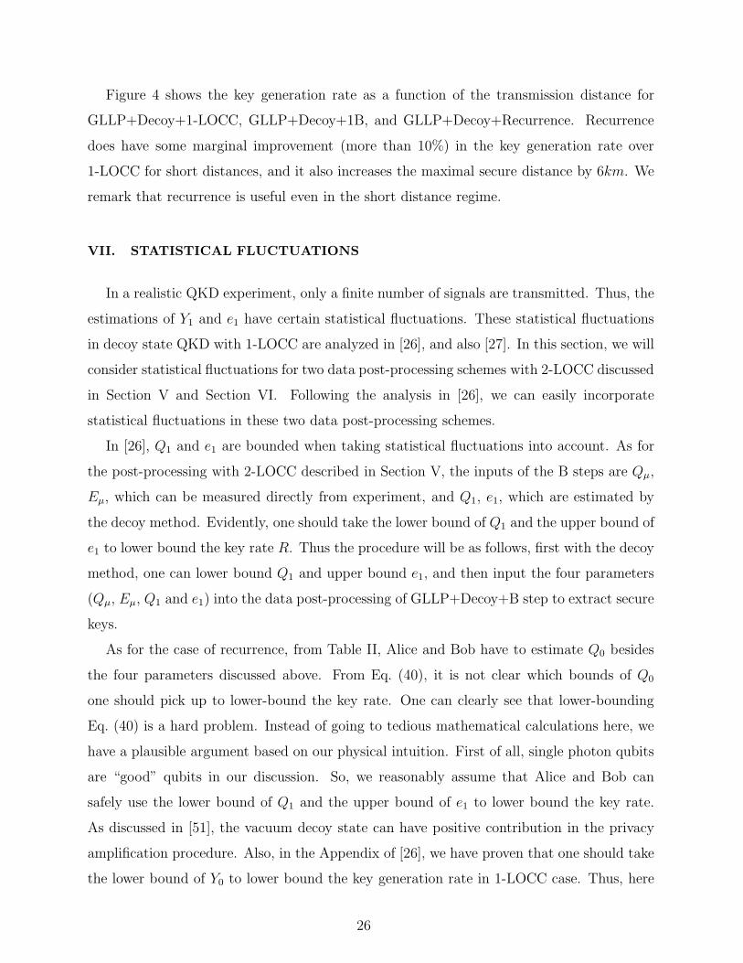
Figure 4 shows the key generation rate as a function of the transmission distance for

GLLP+Decoy+1-LOCC, GLLP+Decoy+1B, and GLLP+Decoy+Recurrence. Recurrence

does have some marginal improvement (more than 10%) in the key generation rate over

1-LOCC for short distances, and it also increases the maximal secure distance by 6km. We

remark that recurrence is useful even in the short distance regime.

VII. STATISTICAL FLUCTUATIONS

In a realistic QKD experiment, only a finite number of signals are transmitted. Thus, the

estimations of Y1 and e1 have certain statistical fluctuations. These statistical fluctuations

in decoy state QKD with 1-LOCC are analyzed in [26], and also [27]. In this section, we will

consider statistical fluctuations for two data post-processing schemes with 2-LOCC discussed

in Section V and Section VI. Following the analysis in [26], we can easily incorporate

statistical fluctuations in these two data post-processing schemes.

In [26], Q1 and e1 are bounded when taking statistical fluctuations into account. As for

the post-processing with 2-LOCC described in Section V, the inputs of the B steps are Qµ,

Eµ, which can be measured directly from experiment, and Q1, e1, which are estimated by

the decoy method. Evidently, one should take the lower bound of Q1 and the upper bound of

e1 to lower bound the key rate R. Thus the procedure will be as follows, first with the decoy

method, one can lower bound Q1 and upper bound e1, and then input the four parameters

(Qµ, Eµ, Q1 and e1) into the data post-processing of GLLP+Decoy+B step to extract secure

keys.

As for the case of recurrence, from Table II, Alice and Bob have to estimate Q0 besides

the four parameters discussed above. From Eq. (40), it is not clear which bounds of Q0

one should pick up to lower-bound the key rate. One can clearly see that lower-bounding

Eq. (40) is a hard problem. Instead of going to tedious mathematical calculations here, we

have a plausible argument based on our physical intuition. First of all, single photon qubits

are “good” qubits in our discussion. So, we reasonably assume that Alice and Bob can

safely use the lower bound of Q1 and the upper bound of e1 to lower bound the key rate.

As discussed in [51], the vacuum decoy state can have positive contribution in the privacy

amplification procedure. Also, in the Appendix of [26], we have proven that one should take

the lower bound of Y0 to lower bound the key generation rate in 1-LOCC case. Thus, here

26

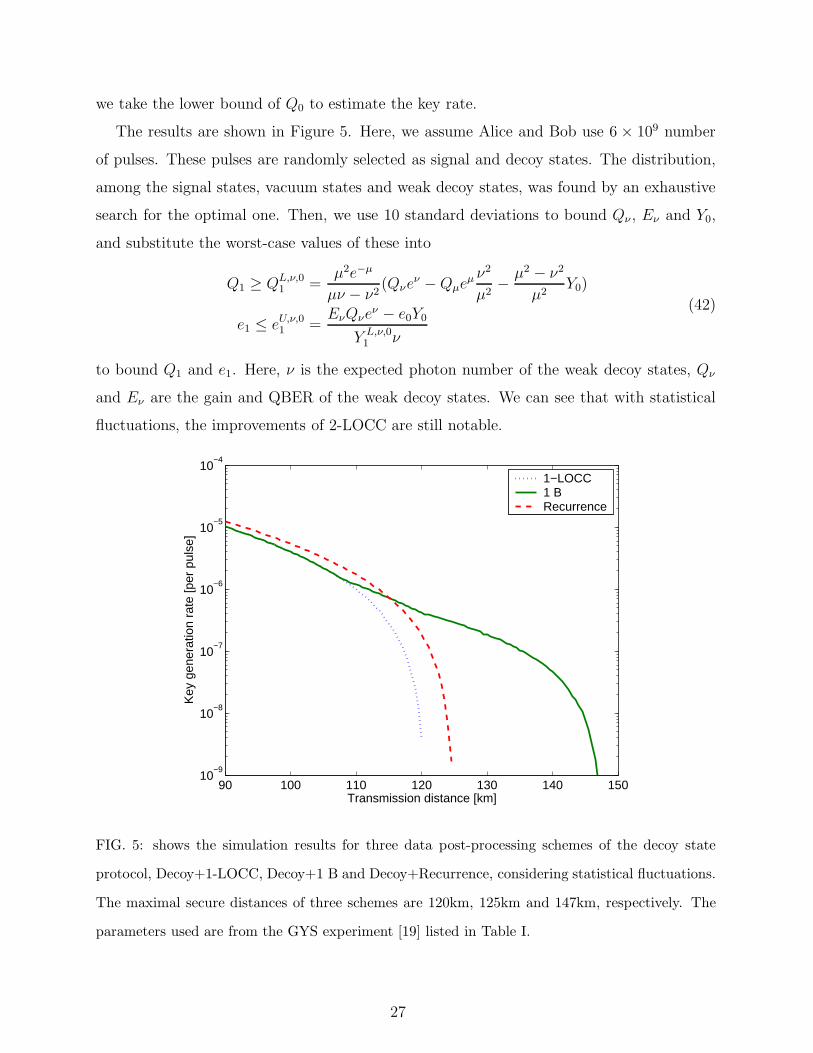
we take the lower bound of Q0 to estimate the key rate.

The results are shown in Figure 5. Here, we assume Alice and Bob use 6 × 109 number

of pulses. These pulses are randomly selected as signal and decoy states. The distribution,

among the signal states, vacuum states and weak decoy states, was found by an exhaustive

search for the optimal one. Then, we use 10 standard deviations to bound Qν , Eν and Y0,

and substitute the worst-case values of these into

Q1 ≥ QL,ν,01 =

µ2e−µ

µν − ν2(Qνe

ν −Qµeµ ν

2

µ2− µ2 − ν2

µ2Y0)

e1 ≤ eU,ν,01 =EνQνe

ν − e0Y0

Y L,ν,01 ν

(42)

to bound Q1 and e1. Here, ν is the expected photon number of the weak decoy states, Qν

and Eν are the gain and QBER of the weak decoy states. We can see that with statistical

fluctuations, the improvements of 2-LOCC are still notable.

90 100 110 120 130 140 15010

−9

10−8

10−7

10−6

10−5

10−4

Transmission distance [km]

Key

gen

erat

ion

rate

[per

pul

se]

1−LOCC1 BRecurrence

FIG. 5: shows the simulation results for three data post-processing schemes of the decoy state

protocol, Decoy+1-LOCC, Decoy+1 B and Decoy+Recurrence, considering statistical fluctuations.

The maximal secure distances of three schemes are 120km, 125km and 147km, respectively. The

parameters used are from the GYS experiment [19] listed in Table I.

27

VIII. CONCLUSION

We have developed two data post-processing schemes for decoy-state QKD using 2-LOCC,

one based on B steps and the other one based on the recurrence method. The distance

of secure QKD is crucial in practical applications. Therefore, our Decoy+B steps post-

processing protocol, which we have shown to be able to increase the maximal secure distance

of QKD from about 141 km to about 182 km (using parameters from the GYS experiment

[19]), proves useful in real-life applications. Moreover, our work shows that recurrence

protocols are useful for increasing the key generation rate in a practical QKD system even

at short distances. While we have focused our modeling on a fiber-based QKD system, our

general formalism applies also to open-air QKD systems.

We have shown that similar conclusions hold even with statistical fluctuations in the

experimental variables for the Decoy+B step scheme. For the Decoy+Recurrence scheme,

although we do not have a rigorous argument, physical intuition suggests that similar con-

clusions hold with statistical fluctuations as well. We conclude that using two-way classical

communications is superior to using one-way for our decoy-state QKD schemes.

In addition, we provided the region of bit error rates and phase error rates that are

tolerable by using the Gottesman-Lo EDP scheme. Also, we calculated the upper bounds

on distance and on the key generation rate of a real QKD setup based on our model.

Acknowledgments

IX. ACKNOWLEDGMENTS

We thank G. Brassard, B. Fortescue, D. Gottesman, and B.Qi for enlightening discussions.

Financial support from CFI, CIAR, CIPI, Connaught, CRC, NSERC, OIT, PREA and the

University of Toronto is gratefully acknowledged.

APPENDIX A: KEY RATE OF THE RECURRENCE SCHEME WITH AN

IDEAL SOURCE

In this section, we review the recurrence EDP and develop the key generation rate formula

given by

R = q · r, (A1)

28

where q depends on the implementation of the QKD (1/2 for the BB84 protocol, because

half the time Alice and Bob bases are not compatible) and r is the residue which we will find

in the sequel. In the following, we use the same notation as in Subsection II and consider a

Bell diagonal state (q00, q10, q11, q01).

a. Parity check

As the first step of recurrence, Alice and Bob check the parity of two pairs (labeled by

control qubit C and target qubit T ). They will get even parity if the two pairs are in one of

the states

0000, 0001, 0100, 0101, 1010, 1011, 1110, 1111,

and will get odd parity if they are in one of the states

0010, 0011, 0110, 0111, 1000, 1001, 1100, 1101,

where the first two bits represent the control qubit, and the last two bits represent the target

qubit. For example, 1110 means that there is a bit error and a phase error in the control

qubit, and a bit error and no phase error in the target qubit. Thus, the probability to get

even parity is given by

pS = (qC00 + qC01)(qT00 + qT01) + (qC10 + qC11)(q

T10 + qT11)

= (1− δCb )(1− δTb ) + δCb δTb ,

(A2)

where δCb = qC10+qC11 and δ

Tb = qT10+q

T11 are the bit error rates of the input control and target

qubits, respectively. During the parity check, the number of pure EPR pairs that Alice and

Bob need to sacrifice is given by1

2H2(pS), (A3)

where 1

2is due to the fact that Alice and Bob compute the parity of two-qubit pairs at one

time.

After the parity check, the qubits are divided into two groups, qubits with even parity and

odd parity. In the following, we will discuss the error correction and privacy amplification

on these two groups separately. The recurrence protocol appearing in [10] only performs

error correction on qubits with even parity.

29

b. Error correction

For even parity qubits, we can see that the bit error syndrome of control qubits will be

the same as that of target qubits. Thus, Alice and Bob only need to do error correction on

the control (or target) qubits. According to Eq. (6), the bit error rate of control qubits after

recurrence is given by

δCb =(qC10 + qC11)(q

T10 + qT11)

pS=δCb δ

Tb

pS(A4)

where pS is the probability of even parity in the recurrence given by Eq. (A2). Therefore,

Alice and Bob need to sacrifice a fraction

1

2pSH2(δ

Cb ) =

1

2pSH2(

δCb δTb

pS) (A5)

to do the overall error correction. The factor 1

2is due to the fact that control qubits have

the same error syndrome as target qubits.

Therefore the residue of data post-processing, similar to Eq. (19), can be expressed as

r = −1

2H2(pS)−

1

2pSH2(

δCb δTb

pS) +K (A6)

where pS is given in Eq. (A2) and K is the residue of privacy amplification, which we will

focus on in the following.

c. Privacy amplification

Alice and Bob perform privacy amplification to the qubits with even and odd parity

separately.

Even parity: now, Alice and Bob already know the bit error syndrome. The control

and target qubits have the same bit error syndromes, but may have different phase error

syndromes. Thus, Alice and Bob can divide the even parity qubits into four groups: control

qubits with bit error syndrome 0 and 1, and target qubits with bit error syndrome 0 and 1,

and treat these groups separately in the privacy amplification step. The probability of each

group (summing together the even parity probabilities given in Eq. (A2)) is given by

(qC00 + qC01)(qT00 + qT01)

2,(qC10 + qC11)(q

T10 + qT11)

2,(qC00 + qC01)(q

T00 + qT01)

2,(qC10 + qC11)(q

T10 + qT11)

2

with phase error rateqC01

qC00 + qC01,

qC11qC10 + qC11

,qT01

qT00 + qT01,

qT11qT10 + qT11

.

30

Since the error syndrome of each group of qubits is known to Alice and Bob, privacy am-

plification can be applied to the different groups separately. Then, Alice and Bob should

sacrifice a fraction

(qC00 + qC01)(qT00 + qT01)

2H2(

qC01qC00 + qC01

) +(qC10 + qC11)(q

T10 + qT11)

2H2(

qC11qC10 + qC11

)+

(qC00 + qC01)(qT00 + qT01)

2H2(

qT01qT00 + qT01

) +(qC10 + qC11)(q

T10 + qT11)

2H2(

qT11qT10 + qT11

)

(A7)

to do the privacy amplification. Given the bit and phase error rates of input control and

target qubits δCp = qC11 + qC01 and δTp = qT11 + qT01, Eq. (A7) can be written as

1

2(1− δCb )(1− δTb )[H2(

δCp − qC111− δCb

) +H2(δTp − qT111− δTb

)] +1

2δCb δ

Tb [H2(

qC11δCb

) +H2(qT11δTb

)]. (A8)

Thus the privacy amplification residue of even parity qubits is given by,

Keven = pS − 1

2(1− δCb )(1− δTb )[H2(

δCp − qC111− δCb

) +H2(δTp − qT111− δTb

)]− 1

2δCb δ

Tb [H2(

qC11δCb

) +H2(qT11δTb

)].

(A9)

Odd parity: it turns out that pairs with odd parity during the recurrence can also

contribute to the final key [10]. Instead of including them in the error correction, Alice

and Bob measure one of the two qubits and hence they know the bit error syndrome of the

remaining qubit. They can then proceed with privacy amplification on those qubits.

Suppose Alice and Bob always choose to measure the target qubits and obtain the error

syndrome of the control qubits. Similar to the even parity case, now, Alice and Bob can

divide the control qubits with odd parity into two parts according to the bit error syndrome.

The probability of each part is given by

(qC00 + qC01)(qT10 + qT11)

2,(qC10 + qC11)(q

T00 + qT01)

2,

with phase error rateqC01

qC00 + qC01,

qC11qC10 + qC11

.

With the same argument as Eq. (A7), the number of qubits that need be sacrificed to

privacy amplification is given by

(qC00 + qC01)(qT10 + qT11)

2H2(

qC01qC00 + qC01

) +(qC10 + qC11)(q

T00 + qT01)

2H2(

qC11qC10 + qC11

)

=1

2[(1− δCb )δ

Tb H2(

δCp − qC111− δCb

) + δCb (1− δTb )H2(qC11δCb

)]

(A10)

31

So the privacy amplification residue of odd parity qubits is given by,

Kodd =1

2(1− δCb )δ

Tb [1−H2(

δCp − qC111− δCb

)] +1

2δCb (1− δTb )[1−H2(

qC11δCb

)] (A11)

Therefore, the privacy amplification residue, K in Eq. (A6), by adding Eq. (A9) and

Eq. (A11) and substituting Eq. (A2), is given by

K =Keven +Kodd

=1− 1

2(1− δCb )δ

Tb − 1

2δCb (1− δTb )−

1

2(1− δCb )H2(

δCp − qC111− δCb

)− 1

2δCb H2(

qC11δCb

)

− 1

2(1− δCb )(1− δTb )H2(

δTp − qT111− δTb

)− 1

2δCb δ

Tb H2(

qT11δTb

).

(A12)

Note that there are two free parameters qC11 and qT11 in Eq. (A12), which should be minimized

over to obtain the worst-case key rate.

APPENDIX B: RESIDUE FOR THE DECOY+GLLP+RECURRENCE SCHEME

We calculate the residues, Ki, in Eq. (39) for the five cases: V⊗

S, S⊗

V , S⊗

S,

S⊗

M ,M⊗

S. Here, we apply each case, with parameters shown in Table II into Eq. (A12)

to calculate each Ki.

V⊗

S: the probability of this case is ΩV S = ΩVΩ.

KV S = 1− 1

4− 1

4H2(1− 2qV11)−

1

4H2(2q

V11)−

1

4(1− e1)H2

(

e1 − a

1− e1

)

− 1

4e1H2

(

a

e1

)

≥ 1

4− 1

4(1− e1)H2

(

e1 − a

1− e1

)

− 1

4e1H2

(

a

e1

)

(B1)

with equality when qV11 = 1/4. This is due to the concavity of function H2(·).S⊗

V : the probability of this case is ΩV S = ΩVΩ.

KSV ≥ 1− 1

4− 1

2(1− e1)H2

(

e1 − a

1− e1

)

− 1

2e1H2

(

a

e1

)

− 1

4(1− e1)H2

(

1− 2qV11)

− 1

4e1H2

(

2qV11)

≥ 1

2− 1

2(1− e1)H2

(

e1 − a

1 − e1

)

− 1

2e1H2

(

a

e1

)

(B2)

with equality when qV11 = 1/4.

32

S⊗

S: the probability of this case is ΩV V = Ω2.

KSS = 1− e1(1− e1)−1

2(1− e1)H2

(

e1 − a

1− e1

)

− 1

2e1H2

(

a

e1

)

− 1

2(1− e1)

2H2

(

e1 − a

1− e1

)

− 1

2e21H2

(

a

e1

)

.

(B3)

S⊗

M : the probability of this case is ΩSM = ΩΩM

KSM = 1− 1

2e1(1− eM )− 1

2eM(1− e1)−

1

2(1− e1)H2

(

e1 − a

1− e1

)

− 1

2e1H2

(

a

e1

)

− 1

2(1− e1)(1− eM)H2

(

1− 2qM112− 2eM

)

− 1

2e1eMH2

(

qM11eM

)

≥ 1

2− 1

2(1− e1)H2

(

e1 − a

1− e1

)

− 1

2e1H2

(

a

e1

)

,

(B4)

with equality when qM11 = eM/2.

M⊗

S: the probability of this case is ΩMS = ΩMΩ

KMS = 1− 1

2eM(1− e1)−

1

2e1(1− eM)− 1

2(1− eM)H2

(

1− 2qM112− 2eM

)

− 1

2eMH2

(

qM11eM

)

− 1

2(1− e1)(1− eM)H2

(

e1 − a

1− e1

)

− 1

2e1eMH2

(

a

e1

)

≥ 1

2− 1

2eM(1− e1)−

1

2e1(1− eM)

− 1

2(1− e1)(1− eM)H2

(

e1 − a

1− e1

)

− 1

2e1eMH2

(

a

e1

)

,

(B5)

with equality when qM11 = eM/2.

Therefore, after combining GLLP [22], Decoy [25], and Recurrence [10], the data post-

processing residue rate will be given by, substituting Eqs. (B1), (B2), (B3), (B4) and (B5)

33

into Eq. (39),

r =− 1

2f(pS)H2(pS)−

1

2pSf(

δ2

pS)H2(

δ2

pS) +KV S +KSV +KSS +KSM +KMS

≥− 1

2f(pS)H2(pS)−

1

2pSf(

δ2

pS)H2(

δ2

pS)

+ ΩV Ω

[

1

4− 1

4(1− e1)H2

(

e1 − a

1− e1

)

− 1

4e1H2

(

a

e1

)]

+ ΩV Ω

[

1

2− 1

2(1− e1)H2

(

e1 − a

1− e1

)

− 1

2e1H2

(

a

e1

)]

+ Ω2[1− e1(1− e1)−1

2(1− e1)H2

(

e1 − a

1− e1

)

− 1

2e1H2

(

a

e1

)

− 1

2(1− e1)

2H2

(

e1 − a

1− e1

)

− 1

2e21H2

(

a

e1

)

]

+ ΩΩM [1

2− 1

2(1− e1)H2

(

e1 − a

1− e1

)

− 1

2e1H2

(

a

e1

)

]

+ ΩΩM [1

2− 1

2eM (1− e1)−

1

2e1(1− eM)

− 1

2(1− e1)(1− eM)H2

(

e1 − a

1− e1

)

− 1

2e1eMH2

(

a

e1

)

]

(B6)

with equality when qV11 = 1/4 and qM11 = eM/2. In order to simplify this formula, we define

some variables,

B =1

2f(pS)H2(pS) +

1

2pSf(

δ2

pS)H2(

δ2

pS)

C =3

4ΩVΩ + Ω2(1− e1 + e21) +

1

2ΩΩM (2− e1 − eM + 2e1eM)

D1 =3

4ΩVΩ +

1

2Ω2(2− e1) +

1

2ΩΩM (2− eM )

D2 =3

4ΩVΩ +

1

2Ω2(1 + e1) +

1

2ΩΩM (eM + 1)

(B7)

Thus Eq. (40) can be expressed as

r =− B +KV S +KSV +KSS +KSM +KMS

≥− B + C − Fa

(B8)

where

Fa = D1(1− e1)H2(e1 − a

1− e1) +D2e1H2(

a

e1) (B9)

with equality when qV11 = 1/4 and qM11 = eM/2.

To lower bound r in Eq. (B8), we need to find the maximum value of Fa over the free

variable a. We are interested in the range of a ∈ [0, e1] with e1 ≤ 1/2. Note that Fa is

34

a concave function of a in the valid range, since a sum of two concave functions is also a

concave function, and reflecting and shifting a concave function is also a concave function.

Thus, we can take the derivative of Fa with respect to a and set it to zero to find the

maximum of Fa. Differentiating Fa with respect to a gives

dFa

da= D1

[

log2

(

e1 − a

1− e1

)

− log2

(

1− e1 − a

1− e1

)]

+D2

[

log2

(

1− a

e1

)

− log2

(

a

e1

)]

Setting 2dFa

da = 1 gives

(

1− e1e1 − a

− 1

)−D1 (e1a

− 1)D2

= 1.

Denoting the left-hand side to be f(a), f(a) is a decreasing function of a since dFa

dais a

decreasing function of a. Therefore, we can use the bisection method to find a such that

f(a) = 1. The initial range for the bisection method is [0, e1].

[1] C. H. Bennett and G. Brassard, “Quantum cryptography: Public key distribution and coin

tossing”, Proceedings of IEEE International Conference on Computers, Systems, and Signal

Processing, Bangalore, India, (IEEE, New York, 1984), pp. 175-179.

[2] D. Mayers, J. of ACM 48, 351 (2001). A preliminary version in D. Mayers, Advances in

Cryptology–Proc. Crypto ’96, vol. 1109 of Lecture Notes in Computer Science, N. Koblitz, Ed.

(Springer-Verlag, New York, 1996), pp. 343-357; E. Biham, M. Boyer, P. O. Boykin, T. Mor,

and V. Roychowdhury, Proceedings of the Thirty-Second Annual ACM Symposium on Theory

of Computing (STOC’00) (ACM Press, New York, 2000), pp. 715-724

[3] H.-K. Lo and H. F. Chau, “Unconditional security of quantum key distribution over arbitrarily

long distances”, Science 283, 2050-2056 (1999).

[4] P. W. Shor and J. Preskill, “Simple proof of security of the BB84 quantum key distribution

protocol”, Phys. Rev. Lett. 85, 441 (2000).

[5] A. K. Ekert, and B. Huttner, J. of Modern Optics 41, 2455 (1994); D. Deutsch et al., Phys.

Rev. Lett. 77, 2818 (1996); Erratum: Phys. Rev. Lett. 80, 2022 (1998).

[6] C. H. Bennett, G. Brassard, S. Popescu, B. Schumacher, J. A. Smolin, and W. K. Wootters,

“Purification of noisy entanglement and faithful teleportation via noisy channels”, Phys. Rev.

Lett. 76, 722-725 (1996), arXiv:quantph/9511027. Erratum: Phys. Rev. Lett. 78, 2031 (1997).

35

[7] D. Deutsch, A. Ekert, R. Jozsa, C. Macchiavello, S. Popescu, and A. Sanpera, “Quantum

privacy amplification and the security of quantum cryptography over noisy channels”, Phys.

Rev. Lett., 77, 2818 (1996). Erratum Phys. Rev. Lett. 80, 2022 (1998).

[8] D. Gottesman and H.-K. Lo, “Proof of security of quantum key distribution with two-way

classical communications”, IEEE Trans. Info. Th., 49(2), 457-475 (2003).

[9] H. F. Chau, “Practical scheme to share a secret key through a quantum channel with a 27.6%

bit error rate”, Phys. Rev. A 66, 060302(R) (2002).

[10] K. Gerd, H. Vollbrecht and F. Verstraete “Interpolation of recurrence and hashing entangle-

ment distillation protocols”, Phys. Rev. A 71, 062325 (2005).

[11] M. Ben-Or, “Simple security proof for quantum key distribution”, presentation available on-

line at http://www.msri.org/publications/ln/msri/2002/qip/ben-or/1/index.html.

[12] R. Renner and R. Koenig, “Universally composable privacy amplification against quantum

adversaries”, Theory of Cryptography: Second Theory of Cryptography Conference, TCC

2005, J.Kilian (ed.) Springer Verlag 2005, vol. 3378 of Lecture Notes in Computer Science,

pp. 407, available on-line at http://arxiv.org/abs/quant-ph/0403133.

[13] M. Christandl, R. Renner and A. Ekert, “A Generic Security Proof for Quantum Key Distri-

bution”, available on-line at http://arxiv.org/abs/quant-ph/0402131.

[14] K. Horodecki, D. Leung, H.-K. Lo and J. Oppenheim, “Quantum Key Distribution Based on

Arbitrarily Weak Distillable Entangled States”, Phys. Rev. Lett., 96, 070501 (2006).

[15] R. Renner, N. Gisin, B. Kraus, “Information-theoretic security proof for quantum-key-

distribution protocols”, Phys. Rev. A 72, 012332 (2005).

[16] M. Ben-Or, Michal Horodecki, D. W. Leung, D. Mayers, J. Oppenheim, Theory of Cryp-

tography: Second Theory of Cryptography Conference, TCC 2005, J.Kilian (ed.) Springer

Verlag 2005, vol. 3378 of Lecture Notes in Computer Science, pp. 386-406, available on-line

at http://arxiv.org/abs/quant-ph/0409078.

[17] MagiQ Technologies, Inc. website: http://www.magiqtech.com/ and id Quantique website:

http://www.idquantique.com/.

[18] C. H. Bennett, F. Bessette, G. Brassard, L. Salvail, and J. Smolin, “Experimental Quantum

Cryptography”, J. Cryptology, 5, 3-28.

[19] C. Gobby, Z. L. Yuan, and A. J. Shields, “Quantum key distribution over 122 km of standard

telecom fiber”, Applied Physics Letters, 84, 3762 (2004).

36

[20] Kimura, T. et al., “Single-photon Interference over 150 km Transmission Using Silica-

based Integrated-optic Interferometers for Quantum Cryptography, On-line available at

http://arxiv.org/quant-ph/0403104.

[21] H. Inamori, N. Lutkenhaus, D. Mayers, “Unconditional Security of Practical Quantum Key

Distribution”, Los Alamos e-Print archive (available at http://arxiv.org/quant-ph/0107017).

[22] D. Gottesman, H.-K. Lo, Norbert Lutkenhaus, and John Preskill, “Security of quantum key

distribution with imperfect devices”, Quantum Information and Computation 4, 325 (2004),

ArXiv:quant-ph/0212066.

[23] M. Koashi, “Unconditional security of coherent-state quantum key distribution with strong

phase-reference pulse”, Phys. Rev. Lett. 93, 120501 (2004).

[24] W.-Y. Hwang, “Quantum Key Distribution with High Loss: Toward Global Secure Communi-

cation”, Phys. Rev. Lett. 91, 057901 (2003)

[25] H.-K. Lo, X. Ma and K. Chen “Decoy State Quantum Key Distribution”, Phys. Rev. Lett. 94,

230504 (2005).

[26] X. Ma, B. Qi, Y. Zhao and H.-K. Lo, “Practical Decoy State for Quantum Key Distribution”,

Phys. Rev. A 72, 012326 (2005)

[27] Xiang-Bin Wang, “Beating the PNS attack in practical quantum cryptography”, Phys. Rev.

Lett. 94, 230503 (2005) and “A decoy-state protocol for quantum cryptography with 4 inten-

sities of coherent states”, Phys. Rev. A 72, 012322 (2005).

[28] J. W. Harrington, J. M. Ettinger, R. J. Hughes, and J. E. Nordholt, “Enhancing

practical security of quantum key distribution with a few decoy states”, available at

http://arxiv.org/abs/quant-ph/0503002

[29] Y. Zhao, B. Qi, X. Ma, H.-K. Lo, and L. Qian “Experimental Quantum Key Distribution with

Decoy States”, , Phys. Rev. Lett. 96, 070502 (2006).

[30] A. Khalique, G. M. Nikolopoulos, and G. Alber, “Suppression of dark-count effects in practical

quantum key-distribution”, quant-ph/0604025 (2006).

[31] A. R. Calderbank and P. W. Shor, “Good quantum error correcting codes exist”, Phys. Rev.

A, 54, pp. 1098-1105 (1996); A. M. Steane, “Multiple particle interference and quantum error

correction”, Proc. Roy. Soc. Lond. A 452, 2551-2577 (1996).

[32] M. Koashi, “Simple security proof of quantum key distribution via uncertainty principle”,

quant-ph/0505108.

37

[33] C. H. Bennett, D. P. DiVincenzo, J. A. Smolin, and W. K. Wootters, “Mixed state entangle-

ment and quantum error correction”, Phys. Rev. A, 54, 3824 (1996).

[34] Norbert Lutkenhaus, “Security against individual attacks for realistic quantum key distribu-

tion”, Phys. Rev. A 61, 052304 (2000).

[35] Eve can selectively surpass all the single photon signals from Alice, and split all the multi

photon signals, keeping one copy herself and send the other copy to Bob. In this way, Eve

could have an identical copy of what Bob processes, thus breaking the security of BB84

protocol.

[36] B. Huttner, N. Imoto, N. Gisin, and T. Mor, “Quantum cryptography with coherent states”,

Phys. Rev. A 51, 1863 (1995).

[37] G. Brassard, N. Lutkenhaus, T. Mor, and B. Sanders, “Security Aspects of Practical Quantum

Cryptography”, Phys. Rev. Lett. 85, 1330 (2000).

[38] Norbert Lutkenhaus, Mika Jahma, “Quantum key distribution with realistic states: photon-

number statistics in the photon-number splitting attack”, New Journal of Physics 4, 44.1-44.9,

(2002).

[39] A. K. Ekert, “Quantum cryptography based on Bell’s theorem”, Phys. Rev. Lett. 67, 661

(1991).

[40] Charles H. Bennett, “Quantum cryptography using any two nonorthogonal states”, Phys. Rev.

Lett. 68, 3121 (1992).

[41] D. Bruss, “Optimal eavesdropping in quantum cryptography with six states”, Phys. Rev. Lett.

81, 3018 (1998).

[42] V. Scarani, A. Acin, G. Ribordy, and N. Gisin, “Quantum Cryptography Protocols Robust

against Photon Number Splitting Attacks for Weak Laser Pulse Implementations”, Phys. Rev.

Lett. 92, 057901 (2004).

[43] K. Tamaki and H.-K. Lo, “Unconditionally secure key distillation from multiphotons”,

Phys. Rev. A. 73, 010302(R) (2006), arXiv:quant-ph/0412035.

[44] C.-H. F. Fung, K. Tamaki, and H.-K. Lo, “Performance of two quantum-key-distribution

protocols”, Phys. Rev. A. 73, 012337 (2006).

[45] U. M. Maurer and S. Wolf, “Unconditionally secure key agreement and the intrinsic conditional

information”, IEEE Trans. Inf. Theory 45, 499 (1999).

[46] G. Brassard and L. Salvail, “Secret-key reconciliation by public discussion”, Advances in Cryp-

38

tology EUROCRYPT ’93, May 1993.

[47] H.-K. Lo, H. F. Chau, and M. Ardehali, “Efficient Quantum Key Distribution Scheme And

Proof of Its Unconditional Security”, J. Cryptology 18, 133-165 (2005).

[48] E.N. Maneva and J.A. Smolin, “Improved two-party and multi-party purification protocols”,

quant-ph/0003099 (2000).

[49] G. Alber, A. Delgado, N. Gisin, I. Jex, “Efficient bipartite quantum state purification in

arbitrary dimensional Hilbert spaces”, J. Phys. A: Math. Gen. 34, 8821-8833, (2001).

[50] J.Dehaene, M. Van den Nest, B. De Moor and F. Verstraete, “Local permutations of products

of Bell states and entanglement distillation”, Phys. Rev. A 67, 022310 (2003).

[51] Hoi-Kwong Lo, “Getting Something Out of Nothing”, Quant. Info. Comp. 5, 413-418 (2005),

arXiv:quant-ph/0503004.

[52] That only single photon qubits contribute to the secure key is only true for a security proof

based on the EDP approach (which is what we use in this paper). It may not be true in other

approaches, e.g., the communication complexity approach, as noted in Ref. [43].

39