arX

iv:q

uant

-ph/

0101

028v

2 6

Jan

200

1

QUANTUM LOGICS

Maria Luisa Dalla Chiara and Roberto Giuntini

February 1, 2008

Contents

1 Introduction 3

2 Orthomodular quantum logic and orthologic 11

3 The implication problem 22

4 Metalogical properties and anomalies 28

5 A modal interpretation of OL and OQL 32

6 An axiomatization of OL and OQL 35

7 The intractability of orthomodularity 40

8 Hilbert quantum logic and the orthomodular law 45

9 First-order quantum logic 50

10 Quantum set theories and theories of quasisets 56

11 The unsharp approaches 59

12 Effect structures 61

13 Paraconsistent quantum logic 70

14 The Brouwer-Zadeh logics 74

15 Partial quantum logics 86

16 Lukasiewicz quantum logic 92

17 Conclusion 96

List of Figures

1 Failure of bivalence in QT . . . . . . . . . . . . . . . . . . . . 82 Quasi-model for γ . . . . . . . . . . . . . . . . . . . . . . . . 313 The Greechie diagram of G12 . . . . . . . . . . . . . . . . . . 464 The orthomodular lattice G12 . . . . . . . . . . . . . . . . . . 47

1

5 The Greechie diagram of B30 . . . . . . . . . . . . . . . . . . 476 G14 . . . . . . . . . . . . . . . . . . . . . . . . . . . . . . . . . 747 M4 . . . . . . . . . . . . . . . . . . . . . . . . . . . . . . . . . 948 M3 . . . . . . . . . . . . . . . . . . . . . . . . . . . . . . . . . 95

2

1 Introduction

The official birth of quantum logic is represented by a famous article ofBirkhoff and von Neumann “The logic of quantum mechanics” (Birkhoffand von Neumann 1936). At the very beginning of their paper, Birkhoffand von Neumann observe:

One of the aspects of quantum theory which has attracted themost general attention, is the novelty of the logical notions whichit presupposes .... The object of the present paper is to discoverwhat logical structures one may hope to find in physical theorieswhich, like quantum mechanics, do not conform to classical logic.

In order to understand the basic reason why a non classical logic arisesfrom the mathematical formalism of quantum theory (QT), a comparisonwith classical physics will be useful.

There is one concept which quantum theory shares alike withclassical mechanics and classical electrodynamics. This is theconcept of a mathematical “phase-space”. According to thisconcept, any physical system S is at each instant hypotheticallyassociated with a “point” in a fixed phase-space Σ; this pointis supposed to represent mathematically, the “state” of S, andthe “state” of S is supposed to be ascertainable by “maximal”observations.

Maximal pieces of information about physical systems are called also purestates. For instance, in classical particle mechanics, a pure state of a sin-gle particle can be represented by a sequence of six real numbers 〈r1, . . . , r6〉where the first three numbers correspond to the position-coordinates, whereasthe last ones are the momentum-components.

As a consequence, the phase-space of a single particle system can beidentified with the set IR6, consisting of all sextuples of real numbers. Sim-ilarly for the case of compound systems, consisting of a finite number n ofparticles.

Let us now consider an experimental proposition P about our system,asserting that a given physical quantity has a certain value (for instance:“the value of position in the x-direction lies in a certain interval”). Sucha proposition P will be naturally associated with a subset X of our phase-space, consisting of all the pure states for which P holds. In other words,the subsets of Σ seem to represent good mathematical representatives ofexperimental propositions. These subsets are called by Birkhoff and von

3

Neumann physical qualities (we will say simply events). Needless to say,the correspondence between the set of all experimental propositions and theset of all events will be many-to-one. When a pure state p belongs to anevent X, we will say that our system in state p verifies both X and thecorresponding experimental proposition.

What about the structure of all events? As is well known, the power-setof any set is a Boolean algebra. And also the set F(Σ) of all measurablesubsets of Σ (which is more tractable than the full power-set of Σ) turns outto have a Boolean structure. Hence, we may refer to the following Booleanalgebra:

B = 〈F(Σ) ,⊆ ,∩ ,∪ , − ,1 ,0〉 ,

where:

1) ⊆ ,∩ ,∪ , − are, respectively, the set-theoretic inclusion relation andthe operations intersection, union, relative complement;

2) 1 is the total space Σ, while 0 is the empty set.

According to a standard interpretation, ∩ ,∪ , − can be naturally re-garded as a set-theoretic realization of the classical logical connectives and ,or , not . As a consequence, we will obtain a classical semantic behaviour:

• a state p verifies a conjunction X ∩ Y iff p ∈ X ∩ Y iff p verifies bothmembers;

• p verifies a disjunction X ∪ Y iff p ∈ X ∪ Y iff p verifies at least onemember;

• p verifies a negation −X iff p /∈ X iff p does not verify X.

To what extent can such a picture be adequately extended to QT?Birkhoff and von Neumann observe:

In quantum theory the points of Σ correspond to the so called“wave-functions” and hence Σ is a ... a function-space, usuallyassumed to be Hilbert space.

As a consequence, we immediately obtain a basic difference between thequantum and the classical case. The excluded middle principle holds in

4

classical mechanics. In other words, pure states semantically decide anyevent: for any p and X,

p ∈ X or p ∈ −X.

QT is, instead, essentially probabilistic. Generally, pure states assignonly probability-values to quantum events. Let ψ represent a pure state (awave function) of a quantum system and let P be an experimental proposi-tion (for instance “the spin value in the x-direction is up”). The followingcases are possible:

(i) ψ assigns to P probability-value 1 (ψ(P) = 1);

(ii) ψ assigns to P probability-value 0 (ψ(P) = 0);

(iii) ψ assigns to P a probability-value different from 1 and from 0 (ψ(P) 6=0, 1).

In the first two cases, we will say that P is true (false) for our systemin state ψ. In the third case, P will be semantically indetermined.

Now the question arises: what will be an adequate mathematical rep-resentative for the notion of quantum experimental proposition? The mostimportant novelty of Birkhoff and von Neumann’s proposal is based on thefollowing answer: “The mathematical representative of any experimentalproposition is a closed linear subspace of Hilbert space” (we will say simplya closed subspace) 1. Let H be a (separable) Hilbert space, whose unitaryvectors correspond to possible wave functions of a quantum system. Theclosed subspaces of H are particular instances of subsets of H that are closedunder linear combinations and Cauchy sequences. Why are mere subsets ofthe phase-space not interesting in QT? The reason depends on the super-position principle, which represents one of the basic dividing line betweenthe quantum and the classical case. Differently from classical mechanics,in quantum mechanics, finite and even infinite linear combinations of purestates give rise to new pure states (provided only some formal conditions

1 A Hilbert space is a vector space over a division ring whose elements are the real orthe complex or the quaternionic numbers such that

(i) An inner product ( . , .) that transforms any pair of vectors into an element of thedivision ring is defined;

(ii) the space is metrically complete with respect to the metrics induced by the innerproduct ( . , .).

A Hilbert space H is called separable iff H admits a countable basis.

5

are satisfied). Suppose three pure states ψ ,ψ1 , ψ2 and let ψ be a linearcombination of ψ1 , ψ2:

ψ = c1ψ1 + c2ψ2.

According to the standard interpretation of the formalism, this means thata quantum system in state ψ might verify with probability |c1|

2 those propo-sitions that are certain for state ψ1 and might verify with probability |c2|

2

those propositions that are certain for state ψ2. Suppose now some purestates ψ1, ψ2, . . . each assigning probability 1 to a certain experimentalproposition P, and suppose that the linear combination

ψ =∑

i

ciψi (ci 6= 0)

is a pure state. Then also ψ will assign probability 1 to our propositionP. As a consequence, the mathematical representatives of experimentalpropositions should be closed under finite and infinite linear combinations.The closed subspaces of H are just the mathematical objects that can realizesuch a role.

What about the algebraic structure that can be defined on the set C(H)of all mathematical representatives of experimental propositions (let us callthem quantum events)? For instance, what does it mean negation, con-junction and disjunction in the realm of quantum events? As to negation,Birkhoff and von Neumann’s answer is the following:

The mathematical representative of the negative of any ex-perimental proposition is the orthogonal complement of themathematical representative of the proposition itself.

The orthogonal complement X ′ of a subspaceX is defined as the set of allvectors that are orthogonal to all elements of X. In other words, ψ ∈ X ′ iffψ ⊥ X iff for any φ ∈ X: (ψ, φ) = 0 (where (ψ, φ) is the inner product of ψand φ). From the point of view of the physical interpretation, the orthogonalcomplement (called also orthocomplement) is particularly interesting, sinceit satisfies the following property: for any event X and any pure state ψ,

ψ(X) = 1 iff ψ(X ′) = 0;

ψ(X) = 0 iff ψ(X ′) = 1;

6

In other words, ψ assigns to an event probability 1 (0, respectively) iff ψassigns to the orthocomplement of X probability 0 (1, respectively). As aconsequence, one is dealing with an operation that inverts the two extremeprobability-values, which naturally correspond to the truth-values truth andfalsity (similarly to the classical truth-table of negation).

As to conjunction, Birkhoff and von Neumann notice that this can bestill represented by the set-theoretic intersection (like in the classical case).For, the intersection X∩Y of two closed subspaces is again a closed subspace.Hence, we will obtain the usual truth-table for the connective and :

ψ verifies X ∩ Y iff ψ verifies both members.

Disjunction, however, cannot be represented here as a set-theoretic union.For, generally, the union X ∪ Y of two closed subspaces is not a closed sub-space. In spite of this, we have at our disposal another good representativefor the connective or : the supremum X ⊔ Y of two closed subspaces, thatis the smallest closed subspace including both X and Y . Of course, X ⊔ Ywill include X ∪ Y .

As a consequence, we obtain the following structure

C(H) =⟨

C(H) ,⊑ ,⊓ ,⊔ , ′ ,1 ,0⟩

where ⊑ ,⊓ are the set-theoretic inclusion and intersection; ⊔ , ′ are definedas above; while 1 and 0 represent, respectively, the total space H and thenull subspace (the singleton of the null vector, representing the smallestpossible subspace). An isomorphic structure can be obtained by using asa support, instead of C(H), the set P (H) of all projections P of H. As iswell known projections (i.e. idempotent and self-adjoint linear operators)and closed subspaces are in one-to-one correspondence, by the projectiontheorem. Our structure C(H) turns out to simulate a “quasi-Boolean be-haviour”; however, it is not a Boolean algebra. Something very essential ismissing. For instance, conjunction and disjunction are no more distributive.Generally,

X ⊓ (Y ⊔ Z) 6= (X ⊓ Y ) ⊔ (X ⊓ Z).

It turns out that C(H) belongs to the variety of all orthocomplemented or-thomodular lattices, that are not necessarily distributive.

The failure of distributivity is connected with a characteristic property ofdisjunction in QT. Differently from classical (bivalent) semantics, a quantumdisjunction X ⊔ Y may be true even if neither member is true. In fact, it

7

OO

oo //

X

jjjjjjjjjjjjjjjjjjjjjjjjjjjjjjjjjjjjjjjjjjjjψ77ooooooooooooooo

Y

Figure 1: Failure of bivalence in QT

may happen that a pure state ψ belongs to a subspace X ⊔ Y , even if ψbelongs neither to X nor to Y (see Figure 1).

Such a semantic behaviour, which may appear prima facie somewhatstrange, seems to reflect pretty well a number of concrete quantum situa-tions. In QT one is often dealing with alternatives that are semanticallydetermined and true, while both members are, in principle, strongly un-determined. For instance, suppose we are referring to some one-half spinparticle (say an electron) whose spin may assume only two possible values:either up or down. Now, according to one of the uncertainty principles, thespin in the x direction (spinx) and the spin in the y direction (spiny) rep-resent two strongly incompatible quantities that cannot be simultaneouslymeasured. Suppose an electron in state ψ verifies the proposition “spinx isup”. As a consequence of the uncertainty principle both propositions “spiny

is up” and “spiny is down” shall be strongly undetermined. However thedisjunction “either spiny is up or spiny is down” must be true.

Birkhoff and von Neumann’s proposal did not arouse any immediate in-terest, either in the logical or in the physical community. Probably, thequantum logical approach appeared too abstract for the foundational de-bate about QT, which in the Thirties was generally formulated in a moretraditional philosophical language. As an example, let us only think of the

8

famous discussion between Einstein and Bohr. At the same time, the workof logicians was still mainly devoted to classical logic.

Only twenty years later, after the appearance of George Mackey’s bookMathematical Foundations of Quantum Theory (Mackey 1957), one has wit-nessed a “renaissance period“ for the logico-algebraic approach to QT. Thishas been mainly stimulated by the researches of Jauch, Piron, Varadara-jan, Suppes, Finkelstein, Foulis, Randall, Greechie, Gudder, Beltrametti,Cassinelli, Mittelstaedt and many others. The new proposals are charac-terized by a more general approach, based on a kind of abstraction fromthe Hilbert space structures. The starting point of the new trends can besummarized as follows. Generally, any physical theory T determines a classof event-state systems 〈E , S〉, where E contains the events that may occurto our system, while S contains the states that a physical system describedby the theory may assume. The question arises: what are the abstract con-ditions that one should postulate for any pair 〈E , S〉? In the case of QT,having in mind the Hilbert space model, one is naturally led to the followingrequirement:

• the set E of events should be a good abstraction from the structure ofall closed subspaces in a Hilbert space. As a consequence E should beat least a σ-complete orthomodular lattice (generally non distributive).

• The set S of states should be a good abstraction from the statisticaloperators in a Hilbert space, that represent possible states of physicalsystems. As a consequence, any state shall behave as a probabilitymeasure, that assigns to any event in E a value in the interval [0, 1].Both in the concrete and in the abstract case, states may be either pure(maximal pieces of information that cannot be consistently extended toa richer knowledge) or mixtures (non maximal pieces of information).

In such a framework two basic problems arise:

I) Is it possible to capture, by means of some abstract conditions that arerequired for any event-state pair 〈E , S〉, the behaviour of the concreteHilbert space pairs?

II) To what extent should the Hilbert space model be absolutely binding?

The first problem gave rise to a number of attempts to prove a kind ofrepresentation theorem. More precisely, the main question was: what arethe necessary and sufficient conditions for a generic event-state pair 〈E , S〉that make E isomorphic to the lattice of all closed subspaces in a Hilbertspace?

9

Our second problem stimulated the investigation about more and moregeneral quantum structures. Of course, looking for more general structuresseems to imply a kind of discontent towards the standard quantum logicalapproach, based on Hilbert space lattices. The fundamental criticisms thathave been moved concern the following items:

1) The standard structures seem to determine a kind of extensional col-lapse. In fact, the closed subspaces of a Hilbert space represent atthe same time physical properties in an intensional sense and the ex-tensions thereof (sets of states that certainly verify the properties inquestion). As happens in classical set theoretical semantics, there is nomathematical representative for physical properties in an intensionalsense. Foulis and Randall have called such an extensional collapse “themetaphysical disaster” of the standard quantum logical approach.

2) The lattice structure of the closed subspaces automatically renders thequantum proposition system closed under logical conjunction. Thisseems to imply some counterintuitive consequences from the physicalpoint of view. Suppose two experimental propositions that concerntwo strongly incompatible quantities, like “the spin in the x directionis up”, “the spin in the y direction is down”. In such a situation,the intuition of the quantum physicist seems to suggest the followingsemantic requirement: the conjunction of our propositions has no def-inite meaning; for, they cannot be experimentally tested at the sametime. As a consequence, the lattice proposition structure seems to betoo strong.

An interesting weakening can be obtained by giving up the lattice condi-tion: generally the infimum and the supremum are assumed to exist onlyfor countable sets of propositions that are pairwise orthogonal. In the recentquantum logical literature an orthomodular partially ordered set that satis-fies the above condition is simply called a quantum logic. At the same time,by standard quantum logic one usually means the complete orthomodularlattice based on the closed subspaces in a Hilbert space. Needless to ob-serve, such a terminology that identifies a logic with a particular example ofan algebraic structure turns out to be somewhat misleading from the strictlogical point of view. As we will see in the next sections, different forms ofquantum logic, which represent “genuine logics” according to the standardway of thinking of the logical tradition, can be characterized by convenientabstraction from the physical models.

10

2 Orthomodular quantum logic and orthologic

We will first study two interesting examples of logic that represent a natu-ral logical abstraction from the class of all Hilbert space lattices.These arerepresented respectively by orthomodular quantum logic (OQL) and by theweaker orthologic (OL), which for a long time has been also termed min-imal quantum logic. In fact, the name “minimal quantum logic” appearstoday quite inappropriate, since a number of weaker forms of quantum logichave been recently investigated. In the following we will use QL as anabbreviation for both OL and OQL.

The language of QL consists of a denumerable set of sentential literalsand of two primitive connectives: ¬ (not), ∧ (and). The notion of formulaof the language is defined in the expected way. We will use the followingmetavariables: p, q, r, . . . for sentential literals and α, β, γ, . . . for formulas.The connective disjunction (∨ ) is supposed defined via de Morgan’s law:

α ∨ β := ¬ (¬α ∧ ¬β) .

The problem concerning the possibility of a well behaved conditional con-nective will be discussed in the next Section. We will indicate the basicmetalogical constants as follows: not, and, or, y (if...then), iff (if and onlyif), ∀ (for all ), ∃ (for at least one).

Because of its historical origin, the most natural characterization of QL

can be carried out in the framework of an algebraic semantics. It will beexpedient to recall first the definition of ortholattice:

Definition 2.1 Ortholattice.An ortholattice is a structure B = 〈B ,⊑ , ′ ,1 ,0〉, where

(2.1.1) 〈B ,⊑ ,1 ,0〉 is a bounded lattice, where 1 is the maximum and0 is the minimum. In other words:

(i) ⊑ is a partial order relation on B (reflexive, antisymmetricand transitive);

(ii) any pair of elements a, b has an infimum a⊓b and a supremuma ⊔ b such that:a ⊓ b ⊑ a, b and ∀c: c ⊑ a, b y c ⊑ a ⊓ b;a, b ⊑ a ⊔ b and ∀c: a, b ⊑ c y a ⊔ b ⊑ c;

(iii) ∀a: 0 ⊑ a; a ⊑ 1.

(2.1.2) the 1-ary operation ′ (called orthocomplement) satisfies the fol-lowing conditions:

11

(i) a′′ = a (double negation);

(ii) a ⊑ b y b′ ⊑ a′ (contraposition);

(iii) a ⊓ a′ = 0 (non contradiction).

Differently from Boolean algebras, ortholattices do not generally satisfythe distributive laws of ⊓ and ⊔. There holds only

(a ⊓ b) ⊔ (a ⊓ c) ⊑ a ⊓ (b ⊔ c)

and the dual form

a ⊔ (b ⊓ c) ⊑(a ⊔ b) ⊓ (a ⊔ c).

The lattice 〈C(H) ,⊑ , ′ ,1 ,0〉 of all closed subspaces in a Hilbert spaceH is a characteristic example of a non distributive ortholattice.

Definition 2.2 Algebraic realization for OL.An algebraic realization for OL is a pair A = 〈B , v〉, consisting of an or-tholattice B = 〈B ,⊑ , ′ ,1 ,0〉 and a valuation-function v that associates toany formula α of the language an element (truth-value) in B, satisfying thefollowing conditions:

(i) v(¬β) = v(β)′;

(ii) v(β ∧ γ) = v(β) ⊓ v(γ).

Definition 2.3 Truth and logical truth.A formula α is true in a realization A = 〈B , v〉 (abbreviated as |=A α) iffv(α) = 1;α is a logical truth of OL (|=

OLα) iff for any algebraic realization A = 〈B , v〉,

|=A α.

When |=A α, we will also say that A is a model of α; A will be called amodel of a set of formulas T (|=A T ) iff A is a model of any β ∈ T .

Definition 2.4 Consequence in a realization and logical consequence.Let T be a set of formulas and let A = 〈B , v〉 be a realization. A formula αis a consequence in A of T (T |=A α) iff for any element a of B:if for any β ∈ T , a ⊑ v(β) then a ⊑ v(α).A formula α is a logical consequence of T (T |=

OLα) iff for any algebraic

realization A: T |=A α.

12

Instead of α |=OLβ we will write α |=

OLβ. If T is finite and equal to

α1, . . . , αn, we will obviously have: T |=OLα iff v(α1)⊓ · · · ⊓ v(αn) ⊑ v(α).

One can easily check that |=OLα iff for any T , T |=

OLα.

OL can be equivalently characterized also by means of a Kripke-stylesemantics, which has been first proposed by Dishkant (1972). As is wellknown, the algebraic semantic approach can be described as founded on thefollowing intuitive idea: interpreting a language essentially means associat-ing to any sentence α an abstract truth-value or, more generally, an abstractmeaning (an element of an algebraic structure). In the Kripkean semantics,instead, one assumes that interpreting a language essentially means associ-ating to any sentence α the set of the possible worlds or situations whereα holds. This set, which represents the extensional meaning of α, is calledthe proposition associated to α (or simply the proposition of α). Hence,generally, a Kripkean realization for a logic L will have the form:

K =⟨

I ,−→Ri ,−→oj ,Π , ρ

⟩

,

where

(i) I is a non-empty set of possible worlds possibly correlated by relationsin the sequence

−→Ri and operations in the sequence −→oj . In most cases,

we have only one binary relation R, called accessibility relation.

(ii) Π is a set of sets of possible worlds, representing possible propositionsof sentences. Any proposition and the total set of propositions Π mustsatisfy convenient closure conditions that depend on the particularlogic.

(iii) ρ transforms sentences into propositions preserving the logical form.

The Kripkean realizations that turn out to be adequate for OL have onlyone accessibility relation, which is reflexive and symmetric. As is well known,many logics, that are stronger than positive logic, are instead characterizedby Kripkean realizations where the accessibility relation is at least reflexiveand transitive. As an example, let us think of intuitionistic logic. From anintuitive point of view, one can easily understand the reason why semanticmodels with a reflexive and symmetric accessibility relation may be physi-cally significant. In fact, physical theories are not generally concerned withpossible evolutions of states of knowledge with respect to a constant world,but rather with sets of physical situations that may be similar , where statesof knowledge must single out some invariants. And similarity relations arereflexive and symmetric, but generally not transitive.

13

Let us now introduce the basic concepts of a Kripkean semantics for OL.

Definition 2.5 Orthoframe.An orthoframe is a relational structure F = 〈I,R 〉, where I is a non-emptyset (called the set of worlds) and R (the accessibility relation) is a binaryreflexive and symmetric relation on I.

Given an orthoframe, we will use i, j, k, . . . as variables ranging over theset of worlds. Instead of Rij (not Rij) we will also write i ⊥/ j (i ⊥ j).

Definition 2.6 Orthocomplement in an orthoframe.Let F = 〈I,R 〉 be an orthoframe. For any set of worlds X ⊆ I, the ortho-complement X ′ of X is defined as follows:

X ′ = i | ∀j(j ∈ X y j ⊥ i) .

In other words, X is the set of all worlds that are unaccessible to all elementsof X. Instead of i ∈ X ′, we will also write i ⊥ X (and we will read it as “iis orthogonal to the set X”). Instead of i /∈ X ′, we will also write i ⊥/ X.

Definition 2.7 Proposition.Let F = 〈I,R 〉 be an orthoframe. A set of worlds X is called a propositionof F iff it satisfies the following condition:

∀i [i ∈ X iff ∀j(i ⊥/ j y j ⊥/ X)] .

In other words, a proposition is a set of worlds X that contains all andonly the worlds whose accessible worlds are not unaccessible to X. Noticethat the conditional i ∈ X y ∀j(i ⊥/ j y j ⊥/ X) trivially holds for any setof worlds X.

Our definition of proposition represents a quite general notion of “possi-ble meaning of a formula”, that can be significantly extended also to otherlogics. Suppose for instance, a Kripkean frame F = 〈I,R 〉, where the ac-cessibility relation is at least reflexive and transitive (as happens in theKripkean semantics for intuitionistic logic). Then a set of worlds X turnsout to be a proposition (in the sense of Definition 2.7) iff it is R-closed (i.e.,∀ij(i ∈ X and Rij y j ∈ X)). And R-closed sets of worlds represent pre-cisely the possible meanings of formulas in the Kripkean characterization ofintuitionistic logic.

Lemma 2.1 Let F be an orthoframe and X a set of worlds of F .

14

(2.1.1) X is a proposition of F iff ∀i [i /∈ X y ∃j(i ⊥/ j and j ⊥ X)]

(2.1.2) X is a proposition of F iff X = X ′′.

Lemma 2.2 Let F = 〈I,R 〉 be an orthoframe.

(2.2.1) I and ∅ are propositions.

(2.2.2) If X is any set of worlds, then X ′ is a proposition.

(2.2.3) If C is a family of propositions, then⋂

C is a proposition.

Definition 2.8 Kripkean realization for OL.A Kripkean realization for OL is a system K = 〈I, R ,Π , ρ〉, where:

(i) F = 〈I,R 〉 is an orthoframe and Π is a set of propositions of theframe that contains ∅, I and is closed under the orthocomplement′ and the set-theoretic intersection ∩;

(ii) ρ is a function that associates to any formula α a proposition inΠ, satisfying the following conditions:

ρ(¬β) = ρ(β)′;

ρ(β ∧ γ) = ρ(β) ∩ ρ(γ).

Instead of i ∈ ρ(α), we will also write i |= α (or,i |=K α, in case ofpossible confusions) and we will read:s “α is true in the world i”. If T is aset of formulas, i |= T will mean i |= β for any β ∈ T .

Theorem 2.1 For any Kripkean realization K and any formula α:

i |= α iff ∀j ⊥/ i∃k ⊥/ j (k |= α).

Proof. Since the accessibility relation is symmetric, the left to right im-plication is trivial. Let us prove i |=/α y not∀j ⊥/ i∃k ⊥/ j (k |= α),which is equivalent to i /∈ ρ(α) y ∃j ⊥/ i∀k ⊥/ j (k /∈ ρ(α)). Supposei /∈ ρ(α). Since ρ(α) is a proposition, by Lemma 2.1.1 there holds for acertain j: j ⊥/ i and j ⊥ ρ(α). Let k ⊥/ j, and suppose, by contradiction,k ∈ ρ(α). Since j ⊥ ρ(α), there follows j ⊥ k, against k ⊥/ j. Consequently,∃j ⊥/ i∀k ⊥/ j (k /∈ ρ(α)).

Lemma 2.3 In any Kripkean realization K:

15

(2.3.1) i |= ¬β iff ∀j ⊥/ i (j |=/ β);

(2.3.2) i |= β ∧ γ iff i |= β and i |= γ.

Definition 2.9 Truth and logical truth.A formula α is true in a realization K = 〈I, R ,Π , ρ〉 (abbreviated |=K α)iff ρ(α) = I;α is a logical truth of OL (|=

OLα) iff for any realization K, |=K α.

When |=K α, we will also say that K is a model of α. Similarly in thecase of a set of formulas T .

Definition 2.10 Consequence in a realization and logical consequence.Let T be a set of formulas and let K be a realization. A formula α is aconsequence in K of T (T |=K α) iff for any world i of K, i |= T y i |= α.A formula α is a logical consequence of T (T |=

OLα) iff for any realization K:

T |=K α. When no confusion is possible we will simply write T |= α.

Now we will prove that the algebraic and the Kripkean semantics for OL

characterize the same logic. Let us abbreviate the metalogical expressions“α is a logical truth of OL according to the algebraic semantics”, “α isa logical consequence in OL of T according to the algebraic semantics”,“α is a logical truth of OL according to the Kripkean semantics”, “α is alogical consequence in OL of T according to the Kripkean semantics”, by

|=A

OLα , T |=

A

OLα , |=

K

OLα , T |=

K

OLα, respectively.

Theorem 2.2 |=A

OLα iff |=

K

OLα, for any α.

The Theorem is an immediate corollary of the following Lemma:

Lemma 2.4

(2.4.1) For any algebraic realization A there exists a Kripkean realiza-tion KA such that for any α, |=A α iff |=KA α.

(2.4.2) For any Kripkean realization K there exists an algebraic real-ization AK such that for any α, |=K α iff |=AK α.

Sketch of the proof.(2.4.1) The basic intuitive idea of the proof is the following: any alge-

braic realization can be canonically transformed into a Kripkean realization

16

by identifying the set of worlds with the set of all non-null elements ofthe algebra, the accessibility-relation with the non-orthogonality relation inthe algebra, and finally the set of propositions with the set of all principalquasi-ideals (i.e., the principal ideals, devoided of the zero-element). Moreprecisely, given A = 〈B , v〉, the Kripkean realization KA = 〈I, R ,Π , ρ〉 isdefined as follows:

I = b ∈ B | b 6= 0;

Rij iff i 6⊑ j′;

Π = b ∈ B | b 6= 0 and b ⊑ a | a ∈ B;

ρ(p) = b ∈ I | b ⊑ v(p).

One can easily check that KA is a “good” Kripkean realization; further, thereholds, for any α : ρ(α) = b ∈ B | b 6= 0 and b ⊑ v(α). Consequently,|=A α iff |=KA α.

(2.4.2) Any Kripkean realization K = 〈I, R ,Π , ρ〉 can be canonicallytransformed into an algebraic realization AK = 〈B , v〉 by putting:

B = Π;

for any a, b ∈ B: a ⊑ b iff a ⊆ b;

a′ = i ∈ I | i ⊥ a;

1 = I; 0 = ∅;

v(p) = ρ(p).

It turns out that B is an ortholattice. Further, for any α, v(α) = ρ(α).Consequently: |=K α iff |=AK α.

Theorem 2.3 T |=A

OLα iff T |=

K

OLα.

Proof. In order to prove the left to right implication, suppose by contra-

diction: T |=A

OLα and T |=

K

OL/α. Hence there exists a Kripkean realization

K = 〈I, R ,Π , ρ〉 and a world i of K such that i |= T and i |=/α. One caneasily see that K can be transformed into K = 〈I, R ,Π , ρ〉 where Π is thesmallest subset of the power-set of I, that includes Π and is closed underinfinitary intersection. Owing to Lemma 2.2.3, K is a “good” Kripkeanrealization for OL and for any β, ρ(β) turns out to be the same propositionin K and in K. Consequently, also in K, there holds: i |= T and i |=/α.Let us now consider AK

. The algebra B of AKis complete, because Π is

closed under infinitary intersection. Hence,⋂

ρ(β) | β ∈ T is an element

17

of B. Since i |= β for any β ∈ T , we will have i ∈⋂

ρ(β) | β ∈ T. Thusthere is an element of B, which is less or equal than v(β)(= ρ(β)) for anyβ ∈ T , but is not less or equal than v(α)(= ρ(α)), because i /∈ ρ(α). This

contradicts the hypothesis T |=A

OLα.

The right to left implication is trivial.

Let us now turn to a semantic characterization of OQL. We will firstrecall the definition of orthomodular lattice.

Definition 2.11 Orthomodular lattice.An orthomodular lattice is an ortholattice B = 〈B ,⊑ ,′ ,1 ,0〉 such that forany a, b ∈ B:

a ⊓(

a′ ⊔ (a ⊓ b))

⊑ b.

Orthomodularity clearly represents a weak form of distributivity.

Lemma 2.5 Let B be an ortholattice. The following conditions are equiva-lent:

(i) B is orthomodular.

(ii) For any a, b ∈ B: a ⊑ b y b = a ⊔ (a′ ⊓ b).

(iii) For any a, b ∈ B: a ⊑ b iff a ⊓ (a ⊓ b)′ = 0.

(iv) For any a, b ∈ B: a ⊑ b and a′ ⊓ b = 0 y a = b.

The property considered in (2.5.(iii)) represents a significant weakeningof the Boolean condition:

a ⊑ b iff a ⊓ b′ = 0.

Definition 2.12 Algebraic realization for OQL.An algebraic realization for OQL is an algebraic realization A = 〈B, v〉 forOL, where B is an orthomodular lattice.

The definitions of truth, logical truth and logical consequence in OQL

are analogous to the corresponding definitions of OL.Like OL, also OQL can be characterized by means of a Kripkean se-

mantics.

Definition 2.13 Kripkean realization for OQL.A Kripkean realization for OQL is a Kripkean realization K = 〈I, R ,Π , ρ〉for OL, where the set of propositions Π satisfies the orthomodular property :X 6⊆ Y y X ∩ (X ∩ Y )′ 6= ∅.

18

The definitions of truth, logical truth and logical consequence in OQL

are analogous to the corresponding definitions of OL. Also in the case ofOQL one can show:

Theorem 2.4 |=A

OQLα iff |=

K

OQLα.

The Theorem is an immediate corollary of Lemma 2.4 and of the follow-ing lemma:

Lemma 2.6

(2.6.1) If A is orthomodular then KA is orthomodular;

(2.6.2) If K is orthomodular then AK is orthomodular.

Proof. (2.6.1) We have to prove X 6⊆ Y y X ∩ (X ∩ Y )′ 6= ∅ for anypropositions X,Y of KA. Suppose X 6⊆ Y . By definition of proposition inKA:

X = b | b 6= 0 and b ⊑ x for a given x;

Y = b | b 6= 0 and b ⊑ y for a given y;

Consequently, x 6⊑ y, and by Lemma 2.5: x ⊓ (x ⊓ y)′ 6= 0 , because Ais orthomodular. Hence, x ⊓ (x ⊓ y)′ is a world in KA. In order to proveX ∩ (X ∩ Y )′ 6= ∅, it is sufficient to prove x ⊓ (x ⊓ y)′ ∈ X ∩ (X ∩ Y )′.There holds trivially x ⊓ (x ⊓ y)′ ∈ X. Further, x ⊓ (x ⊓ y)′ ∈ (X ∩ Y )′,because (x ⊓ y)′ is the generator of the quasi-ideal (X ∩ Y )′ . Consequently,x ⊓ (x ⊓ y)′ ∈ X ∩ (X ∩ Y )′.(2.6.2) Let K be orthomodular. Then for any X,Y ∈ Π:

X 6⊆ Y y X ∩ (X ∩ Y )′ 6= ∅.

One can trivially prove:

X ∩ (X ∩ Y )′ 6= ∅ y X 6⊆ Y.

Hence, by Lemma 2.5, the algebra B of AK is orthomodular.

As to the concept of logical consequence, the proof we have given for OL

(Theorem 2.3) cannot be automatically extended to the case of OQL. Thecritical point is represented by the transformation of K into K whose set ofpropositions is closed under infinitary intersection: K is trivially a “good”OL-realization; at the same time, it is not granted that K preserves theorthomodular property. One can easily prove:

19

Theorem 2.5 T |=K

OQLα y T |=

A

OQLα.

The inverse relation has been proved by Minari (1987):

Theorem 2.6 T |=A

OQLα y T |=

K

OQLα.

Are there any significant structural relations between A and KAKand be-

tween K and AKA? The question admits a very strong answer in the case

of A and KAK.

Theorem 2.7 A = 〈B, v〉 and AKA= 〈B∗, v∗〉 are isomorphic realizations.

Sketch of the proof. Let us define the function ψ : B → B∗ in the followingway:

ψ(a) = b | b 6= 0 and b ⊑ a for any a ∈ B.

One can easily check that: (1) ψ is an isomorphism (from B onto B∗); (2)v∗(p) = ψ(v(p)) for any atomic formula p.

At the same time, in the case of K and KAK

, there is no natural cor-respondence between I and Π. As a consequence, one can prove only theweaker relation:

Theorem 2.8 Given K = 〈I ,R ,Π , ρ〉 and KAK

= 〈I∗ , R∗ ,Π∗ , ρ∗〉, thereholds:

ρ∗(α) = X ∈ Π | X ⊆ ρ(α) , for any α.

In the class of all Kripkean realizations for QL, the realizations KA

(which have been obtained by canonical transformation of an algebraic re-alization A) present some interesting properties, which are summarized bythe following theorem.

Theorem 2.9 In any KA = 〈I ,R ,Π , ρ〉 there is a one-to-one correspon-dence φ between the set of worlds I and the set of propositions Π−∅ suchthat:

(2.9.1) i ∈ φ(i);

(2.9.2) i ⊥/ j iff φ(i) 6⊆ φ(j)′;

(2.9.3) ∀X ∈ Π: i ∈ X iff ∀k ∈ φ(i)(k ∈ X).

Sketch of the proof. Let us take as φ(i) the quasi-ideal generated by i.

20

Theorem 2.9 suggests to isolate, in the class of all K, an interestingsubclass of Kripkean realizations, that we will call algebraically adequate.

Definition 2.14 A Kripkean realization K is algebraically adequate iff itsatisfies the conditions of Theorem 2.9.

When restricting to the class of all algebraically adequate Kripkean re-alizations one can prove:

Theorem 2.10 K = 〈I ,R ,Π , ρ〉 and KAK

= 〈I∗ , R∗ ,Π∗ , ρ∗〉 are isomor-phic realizations; i.e., there exists a bijective function ψ from I onto I∗ suchthat:

(2.10.1) Rij iff R∗ψ(i)ψ(j), for any i, j ∈ I;

(2.10.2) Π∗ = ψ(X) | X ∈ Π, where ψ(X) := ψ(i) | i ∈ X;

(2.10.3) ρ∗(p) = ψ(ρ(p)), for any atomic formula p.

One can easily show that the class of all algebraically adequate Krip-kean realizations determines the same concept of logical consequence that isdetermined by the larger class of all possible realizations.

The Kripkean characterization of QL turns out to have a quite naturalphysical interpretation. As we have seen in the Introduction, the mathemat-ical formalism of quantum theory (QT) associates to any physical system Sa Hilbert space H, while pure states of S are mathematically represented byunitary vectors ψ of H. Let us now consider an elementary sublanguage LQ

of QT, whose atomic formulas represent possible measurement reports (i.e.,statements of the form “the value for the observable Q lies in the Borel set∆”) and suppose LQ closed under the quantum logical connectives. Givena physical system S (whose associated Hilbert space is H), one can define anatural Kripkean realization for the language LQ as follows:

KS = 〈I ,R ,Π , ρ〉 ,

where:

• I is the set of all pure states ψ of S.

• R is the non-orthogonality relation between vectors (in other words,two pure states are accessible iff their inner product is different fromzero).

• Π is the set of all propositions that is univocally determined by theset of all closed subspaces of H (one can easily check that the set ofall unitary vectors of any subspace is a proposition).

21

• For any atomic formula p, ρ(p) is the proposition containing all thepure states that assign to p probability-value 1.

Interestingly enough, the accessibility relation turns out to have the fol-lowing physical meaning: Rij iff j is a pure state into which i can betransformed after the performance of a physical measurement that concernan observable of the system.

3 The implication problem

Differently from most weak logics, QL gives rise to a critical “implication-problem”. All conditional connectives one can reasonably introduce in QL

are, to a certain extent, anomalous; for, they do not share most of thecharacteristic properties that are satisfied by the positive conditionals (whichare governed by a logic that is at least as strong as positive logic). Just thefailure of a well-behaved conditional led some authors to the conclusionthat QL cannot be a “real” logic. In spite of these difficulties, these daysone cannot help recognizing that QL admits a set of different implicationalconnectives, even if none of them has a positive behaviour. Let us firstpropose a general semantic condition for a logical connective to be classifiedas an implication-connective.

Definition 3.1 In any semantics, a binary connective∗→ is called an implication-

connective iff it satisfies at least the two following conditions:

(3.1.1) α∗→ α is always true (identity);

(3.1.2) if α is true and α∗→ β is true then β is true (modus ponens).

In the particular case of QL, one can easily obtain:

Lemma 3.1 A sufficient condition for a connective∗→ to be an implication-

connective is:

(i) in the algebraic semantics: for any realization A = 〈A, v〉, |=A α∗→ β

iff v(α) ⊑ v(β);

(ii) in the Kripkean semantics: for any realization K = 〈I,R,Π, ρ〉,

|=K α∗→ β iff ρ(α) ⊆ ρ(β).

In QL it seems reasonable to assume the sufficient condition of Lemma3.1 as a minimal condition for a connective to be an implication-connective.

22

Suppose we have independently defined two different implication-connectivesin the algebraic and in the Kripkean semantics. When shall we admit thatthey represent the “same logical connective”? A reasonable answer to thisquestion is represented by the following convention:

Definition 3.2 LetA∗ be a binary connective defined in the algebraic se-

mantics andK∗ a binary connective defined in the Kripkean semantics:

A∗

andK∗ represent the same logical connective iff the following conditions are

satisfied:

(3.2.1) given any A = 〈B, v〉 and given the corresponding KA = 〈I,R,Π, ρ〉,

ρ(αK∗ β) is the quasi-ideal generated by v(α

A∗ β);

(3.2.2) given any K = 〈I,R,Π, ρ〉 and given the corresponding AK =

〈B , v〉, there holds: v(αA∗ β) = ρ(α

K∗ β).

We will now consider different possible semantic characterizations of animplication-connective in QL. Differently from classical logic, in QL a mate-rial conditional defined by Philo-law (α→ β := ¬α∨β), does not give rise toan implication-connective. For, there are algebraic realizations A = 〈B, v〉such that v(¬α ∨ β) = 1, while v(α) 6⊑ v(β). Further, ortholattices andorthomodular lattices are not, generally, pseudocomplemented lattices: inother words, given a, b ∈ B, the maximum c such that a ⊓ c ⊑ b doesnot necessarily exist in B. In fact, one can prove (Birkhoff 1995) that anypseudocomplemented lattice is distributive.

We will first consider the case of polynomial conditionals, that can bedefined in terms of the connectives ∧ ,∨ ,¬. In the algebraic semantics, theminimal requirement of Lemma 3.1 restricts the choice only to five possiblecandidates (Kalmbach 1983). This result follows from the fact that in theorthomodular lattice freely generated by two elements there are only fivepolynomial binary operations satisfying the condition a ⊑ b iff a b = 1.These are our five candidates:

(i) v(α→1 β) = v(α)′ ⊔ (v(α) ⊓ v(β)).

(ii) v(α→2 β) = v(β) ⊔ (v(α)′ ⊓ v(β)′).

(iii) v(α→3 β) = (v(α)′ ⊓ v(β)) ⊔ (v(α) ⊓ v(β)) ⊔ (v(α)′ ⊓ v(β)′).

(iv) v(α→4 β) = (v(α)′ ⊓ v(β))⊔ (v(α)⊓ v(β))⊔ ((v(α)′ ⊔ v(β))⊓ v(β)′).

(v) v(α→5 β) = (v(α)′⊓v(β))⊔ (v(α)′ ⊓v(β)′)⊔ (v(α)⊓ (v(α)′⊔v(β))).

23

The corresponding five implication-connectives in the Kripkean seman-tics can be easily obtained. It is not hard to see that for any i (1 ≤ i ≤ 5),→i represents the same logical connective in both semantics (in the sense ofDefinition 3.2).

Theorem 3.1 The polynomial conditionals →i (1 ≤ i ≤ 5) are implication-connectives in OQL; at the same time they are not implication-connectivesin OL.

Proof. Since →i represent the same connective in both semantics, it will besufficient to refer to the algebraic semantics. As an example, let us provethe theorem for i = 1 (the other cases are similar). First we have to provev(α) ⊑ v(β) iff 1 = v(α →1 β) = v(α)′ ⊔ (v(α) ⊓ v(β)), which is equivalentto v(α) ⊑ v(β) iff v(α)⊓(v(α)⊓v(β))′ = 0. From Lemma 2.5, we know thatthe latter condition holds for any pair of elements of B iff B is orthomodular.This proves at the same time that →1 is an implication-connective in OQL,but cannot be an implication-connective in OL.

Interestingly enough, each polynomial conditional →i represents a goodweakening of the classical material conditional. In order to show this result,let us first introduce an important relation that describe a “Boolean mutualbehaviour” between elements of an orthomodular lattice.

Definition 3.3 Compatibility.Two elements a, b of an orthomodular lattice B are compatible iff

a = (a ⊓ b′) ⊔ (a ⊓ b).

One can prove that a, b are compatible iff the subalgebra of B generated bya, b is Boolean.

Theorem 3.2 For any algebraic realization A = 〈B, v〉 and for any α, β:

v(α→i β) = v(α)′ ⊔ v(β) iff v(α) and v(β) are compatible.

As previously mentioned, Boolean algebras are pseudocomplemented lat-tices. Therefore they satisfy the following condition for any a, b, c:

c ⊓ a ⊑ b iff c ⊑ a b,

where: a b := a′ ⊔ b.

24

An orthomodular lattice B turns out to be a Boolean algebra iff for anyalgebraic realization A = 〈B, v〉, any i (1 ≤ i ≤ 5) and any α, β the followingimport-export condition is satisfied:

v(γ) ⊓ v(α) ⊑ v(β) iff v(γ) ⊑ v(α→i β).

In order to single out a unique polynomial conditional, various weaken-ings of the import-export condition have been proposed. For instance thefollowing condition (which we will call weak import-export):

v(γ)⊓v(α) ⊑ v(β) iff v(γ) ⊑ v(α) →i v(β), if v(α) and v(β) are compatible.

One can prove (Hardegree 1975, Mittelstaedt 1972) that a polynomialconditional →i satisfies the weak import-export condition iff i = 1. As a con-sequence, we can conclude that →1 represents, in a sense, the best possibleapproximation for a material conditional in quantum logic. This connective(often called Sasaki-hook) was originally proposed by Mittelstaedt (1972)and Finch (1970), and was further investigated by Hardegree (1976) andother authors. In the following, we will usually write → instead of →1 andwe will neglect the other four polynomial conditionals.

Some important positive laws that are violated by our quantum logicalconditional are the following:

α→ (β → α);

(α→ (β → γ)) → ((α → β) → (α→ γ));

(α→ β) → ((β → γ) → (α→ γ));

(α ∧ β → γ) → (α→ (β → γ));

(α→ (β → γ)) → (β → (α→ γ)).

This somewhat “anomalous” behaviour has suggested that one is deal-ing with a kind of counterfactual conditional . Such a conjecture seems tobe confirmed by some important physical examples. Let us consider againthe class of the Kripkean realizations of the sublanguage LQ of QT (whoseatomic sentences express measurement reports). And let KS = 〈I,R,Π, ρ〉represent a Kripkean realization of our language, which is associated to aphysical system S. As Hardegree (1975) has shown, in such a case the con-ditional → turns out to receive a quite natural counterfactual interpretation

25

(in the sense of Stalnaker). More precisely, one can define, for any formulaα, a partial Stalnaker-function function fα in the following way:

fα : Dom(fα) → I,

where:Dom(fα) = i ∈ I | i ⊥/ ρ(α)

In other words, fα is defined for all and only the states that are not orthog-onal to the proposition of α.

If i ∈ Dom(fα), then:

fα(i) = Pρ(α)i,

where Pρ(α) is the projection that is uniquely associated with the closedsubspace determined by ρ(α). There holds:

i |= α→ β iff either ∀j ⊥/ i(j |=/α) or fα(i) |= β.

In other words: should i verify α, then i would verify also β.From an intuitive point of view, one can say that fρ(α)(i) represents the “purestate nearest” to i, that verifies α, where “nearest” is here defined in termsof the metrics of the Hilbert space H. By definition and in virtue of one ofthe basic postulates of QT (von Neumann’s collapse of the wave function),fρ(α) turns out to have the following physical meaning: it represents thetransformation of state i after the performance of a measurement concerningthe physical property expressed by α, provided the result was positive. As aconsequence, one obtains: α→ β is true in a state i iff either α is impossiblefor i or the state into which i has been transformed after a positive α-test,verifies α.

Another interesting characteristic of our connective →, is a weak nonmonotonic behaviour. In fact, in the algebraic semantics the inequality

v(α → γ) ⊑ v(α ∧ β → γ)

can be violated (a counterexample can be easily obtained in the orthomod-ular lattice based on IR3). As a consequence:

α→ γ |=/α ∧ β → γ.

Polynomial conditionals are not the only significant examples of implication-connectives in QL. In the framework of a Kripkean semantic approach, itseems quite natural to introduce a conditional connective, that represents a

26

kind of strict implication. Given a Kripkean realization K = 〈I,R,Π, ρ〉 onewould like to require:

i |= α⊸ β iff ∀j ⊥/ i (j |= α y j |= β).

However such a condition does not automatically represent a correctsemantic definition, because it is not granted that ρ(α⊸ β) is an elementof Π. In order to overcome this difficulty, let us first define a new operationin the power-set of an orthoframe 〈I,R〉.

Definition 3.4 Strict-implication operation ( ⊸ ).Given an orthoframe 〈I,R〉 and X,Y ⊆ I:

X ⊸ Y := i | ∀j (i ⊥/ j and j ∈ X y j ∈ Y ) .

If X and Y are sets of worlds in the orthoframe, then X ⊸ Y turns outto be a proposition of the frame.

When the set Π of K is closed under ⊸ , we will say that K is a realizationfor a strict-implication language.

Definition 3.5 Strict implication (⊸).If K = 〈I,R,Π, ρ〉 is a realization for a strict-implication language, then

ρ(α⊸ β) := ρ(α) ⊸ ρ(β).

One can easily check that ⊸ is a “good” conditional. There followsimmediately:

i |= α⊸ β iff ∀j ⊥/ i (j |= α y j |= β).

Another interesting implication that can be defined in QL is represented byan entailment-connective.

Definition 3.6 Entailment (։).Given K = 〈I,R,Π, ρ〉,

ρ(α։ β) :=

I, if ρ(α) ⊆ ρ(β);

∅, otherwise.

Since I, ∅ ∈ Π, the definition is correct. One can trivially check that ։ isa “good” conditional. Interestingly enough, our strict implication and ourentailment represent “good” implications also for OL.

The general relations between →,⊸ and։ are described by the follow-ing theorem:

27

Theorem 3.3 For any realization K for a strict-implication language ofOL:

|=K (α։ β)։ (α⊸ β).

For any realization K for a strict-implication language of OQL:

|=K (α։ β)։ (α→ β); |=K (α⊸ β)։ (α→ β).

But the inverse relations do not generally hold!Are the connectives⊸ and ։ definable also in the algebraic semantics?

The possibility of defining ։ is straightforward.

Definition 3.7 Entailment in the algebraic semantics.Given A = 〈B, v〉,

v(α։ β) :=

1, if v(α) ⊑ v(β);

0, otherwise.

One can easily check that ։ represents the same connective in the twosemantics. As to ⊸, given A = 〈B, v〉, one would like to require:

v(α⊸ β) =⊔

b ∈ B | b 6= 0 and ∀c(c 6= 0 and b 6⊑ c′ and c ⊑ v(α) y c ⊑ v(β))

.

However such a definition supposes the algebraic completeness of B. Fur-ther we can prove that⊸ represents the same connective in the two seman-tics only if we restrict our consideration to the class of all algebraicallyadequate Kripkean realizations.

4 Metalogical properties and anomalies

Some metalogical distinctions that are not interesting in the case of a numberof familiar logics weaker than classical logic turn out to be significant forQL (and for non distributive logics in general).

We have already defined (both in the algebraic and in the Kripkeansemantics) the concepts of model and of logical consequence. Now we willintroduce, in both semantics, the notions of quasi-model , weak consequenceand quasi-consequence. Let T be any set of formulas.

Definition 4.1 Quasi-model .

28

Algebraic semantics Kripkean semanticsA realization A = 〈B, v〉 A realization K = 〈I,R,Π, ρ〉is a quasi-model of T iff is a quasi-model of T iff∃a[a ∈ B and a 6= 0 and ∃i(i ∈ I and i |= T ).∀β ∈ T (a ⊑ v(β))].

The following definitions can be expressed in both semantics.

Definition 4.2 Realizability and verifiability .T is realizable (RealT ) iff it has a quasi-model; T is verifiable (Verif T ) iffit has a model.

Definition 4.3 Weak consequence.A formula α is a weak consequence of T (T |≡ α) iff any model of T is a

model of α.

Definition 4.4 Quasi-consequence.A formula α is a quasi-consequence of T (T |≈ α) iff any quasi-model of

T is a quasi-model of α.

One can easily check that the algebraic notions of verifiability, realizabil-ity, weak consequence and quasi-consequence turn out to coincide with thecorresponding Kripkean notions. In other words, T is Kripke-realizable iffT is algebraically realizable. Similarly for the other concepts.

In both semantics one can trivially prove the following lemmas.

Lemma 4.1 Verif T y Real T.

Lemma 4.2 Real T iff for any contradiction β ∧ ¬β, T |=/ β ∧ ¬β.

Lemma 4.3 T |= α y T |≡ α; T |= α y T |≈ α.

Lemma 4.4 α |≡ β iff ¬β |≈ ¬α.

Most familiar logics, that are stronger than positive logic, turn out tosatisfy the following metalogical properties, which we will call Herbrand-Tarski , verifiability and Lindenbaum, respectively.

29

• Herbrand-Tarski

T |= α iff T |≡ α iff T |≈ α

• Verifiability

VerT iff Real T

• Lindenbaum

RealT y ∃T ∗ [T ⊆ T ∗ and ComplT ∗], where

ComplT iff ∀α [α ∈ T or ¬α ∈ T ].

The Herbrand-Tarski property represents a semantic version of the de-duction theorem. The Lindenbaum property asserts that any semanticallynon-contradictory set of formulas admits a semantically non-contradictorycomplete extension. In the algebraic semantics, canonical proofs of theseproperties essentially use some versions of Stone-theorem, according to whichany proper filter F in an algebra B can be extended to a proper completefilter F ∗ (such that ∀a(a ∈ F ∗ or a′ ∈ F ∗)). However, Stone-theorem doesnot generally hold for non distributive orthomodular lattices! In the case ofortholattices, one can still prove that every proper filter can be extended toan ultrafilter (i.e., a maximal filter that does not admit any extension thatis a proper filter). However, differently from Boolean algebras, ultrafiltersneed not be complete.

A counterexample to the Herbrand-Tarski property in OL can be ob-tained using the “non-valid” part of the distributive law. We know that(owing to the failure of distributivity in ortholattices):

α ∧ (β ∨ γ) |=/ (α ∧ β) ∨ (α ∧ γ).

At the same time

α ∧ (β ∨ γ) |≡ (α ∧ β) ∨ (α ∧ γ),

since one can easily calculate that for any realization A = 〈B, v〉 the hypoth-esis v(α ∧ (β ∨ γ)) = 1, v((α ∧ β) ∨ (α ∧ γ)) 6= 1 leads to a contradiction 2.

A counterexample to the verifiability-property is represented by thenegation of the a fortiori principle for the quantum logical conditional →:

γ := ¬(α→ (β → α)) = ¬(¬α ∨ (α ∧ (¬β ∨ (α ∧ β)))).

2In OQL a counterexample in two variables can be obtained by using the failureof the contraposition law for →. One has: α → β |=/¬β → ¬α. At the same timeα → β |≡ ¬β → ¬α; since for any realization A = 〈B, v〉 the hypothesis v(α → β) = 1,implies v(α) ⊑ v(β) and therefore v(¬β → ¬α) = v(β)⊔(v(α)′⊓v(β)′) = v(β)⊔v(β)′ = 1.

30

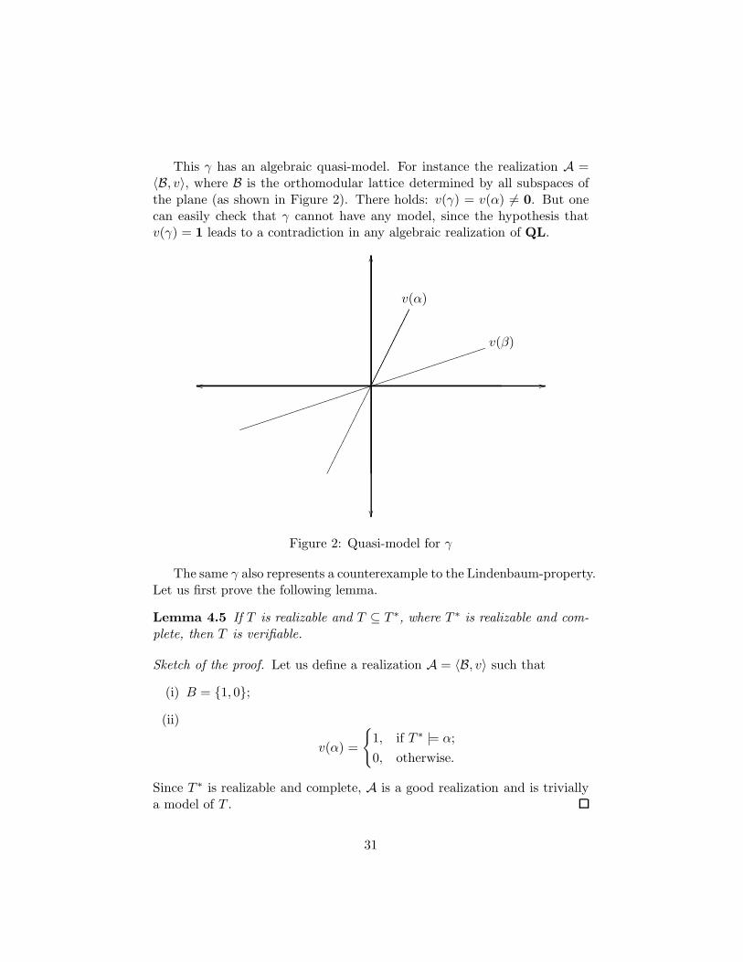
This γ has an algebraic quasi-model. For instance the realization A =〈B, v〉, where B is the orthomodular lattice determined by all subspaces ofthe plane (as shown in Figure 2). There holds: v(γ) = v(α) 6= 0. But onecan easily check that γ cannot have any model, since the hypothesis thatv(γ) = 1 leads to a contradiction in any algebraic realization of QL.

OO

oo //

v(β)

jjjjjjjjjjjjjjjjjjjjjjjjjjjjjjjjjjjjjjjjjjj

v(α)

Figure 2: Quasi-model for γ

The same γ also represents a counterexample to the Lindenbaum-property.Let us first prove the following lemma.

Lemma 4.5 If T is realizable and T ⊆ T ∗, where T ∗ is realizable and com-plete, then T is verifiable.

Sketch of the proof. Let us define a realization A = 〈B, v〉 such that

(i) B = 1, 0;

(ii)

v(α) =

1, if T ∗ |= α;

0, otherwise.

Since T ∗ is realizable and complete, A is a good realization and is triviallya model of T .

31

Now, one can easily show that γ violates Lindenbaum. Suppose, by con-tradiction, that γ has a realizable and complete extension. Then, by Lemma4.5, γ must have a model, and we already know that this is impossible.

The failure of the metalogical properties we have considered represents,in a sense, a relevant “anomaly” of quantum logics. Just these anomaliessuggest the following conjecture: the distinction between epistemic logics(characterized by Kripkean models where the accessibility relation is at leastreflexive and transitive) and similarity logics (characterized by Kripkeanmodels where the accessibility relation is at least reflexive and symmetric)seems to represent a highly significant dividing line in the class of all logicsthat are weaker than classical logic.

5 A modal interpretation of OL and OQL

QL admits a modal interpretation ((Goldblatt 1974), (Dalla Chiara 1981))which is formally very similar to the modal interpretation of intuitionisticlogic. Any modal interpretation of a given non-classical logic turns out tobe quite interesting from the intuitive point of view, since it permits usto associate a classical meaning to a given system of non-classical logicalconstants. As is well known, intuitionistic logic can be translated into themodal system S4. The modal basis that turns out to be adequate for OL isinstead the logic B. Such a result is of course not surprising, since both theB-realizations and the OL-realizations are characterized by frames wherethe accessibility relation is reflexive and symmetric.

Suppose a modal language LM whose alphabet contains the same senten-tial literals as QL and the following primitive logical constants: the classicalconnectives ∼ (not), f (and) and the modal operator (necessarily). Atthe same time, the connectives g (or), ⊃ (if ... then), ≡ (if and only if ),and the modal operator ♦ (possibly) are supposed defined in the standardway.

The modal logic B is semantically characterized by a class of Kripkeanrealizations that we will call B-realizations.

Definition 5.1 A B-realization is a system M = 〈I,R,Π, ρ〉 where:

(i) 〈I,R〉 is an orthoframe;

(ii) Π is a subset of the power-set of I satisfying the following condi-tions:

I, ∅ ∈ Π;

32

Π is closed under the set-theoretic relative complement −,the set-theoretic intersection ∩ and the modal operation ⊡,which is defined as follows:for any X ⊆ I, ⊡X := i | ∀j (Rij y j ∈ X);

(iii) ρ associates to any formula α of LM a proposition in Π satisfyingthe conditions: ρ(∼ β) = −ρ(β); ρ(βfγ) = ρ(β)∩ρ(γ); ρ(β) =⊡ρ(β).

Instead of i ∈ ρ(α), we will write i |= α. The definitions of truth, logicaltruth and logical consequence for B are analogous to the correspondingdefinitions in the Kripkean semantics for QL.

Let us now define a translation τ of the language of QL into the languageLB.

Definition 5.2 Modal translation of OL.

• τ(p) = ♦p;

• τ(¬β) = ∼ τ(β);

• τ(β ∧ γ) = τ(β)f τ(γ).

In other words, τ translates any atomic formula as the necessity of thepossibility of the same formula; further, the quantum logical negation isinterpreted as the necessity of the classical negation, while the quantum log-ical conjunction is interpreted as the classical conjunction. We will indicatethe set τ(β) | β ∈ T by τ(T ).

Theorem 5.1 For any α and T of OL: T |=OLα iff T |=

Bτ(α)

Theorem 5.1 is an immediate corollary of the following Lemmas 5.1 and5.2.

Lemma 5.1 Any OL-realization K = 〈I,R,Π, ρ〉 can be transformed intoa B-realization MK = 〈I∗, R∗,Π∗, ρ∗〉 such that: I∗ = I; R∗ = R;∀i (i |=K α iff i |=MK τ(α)).

Sketch of the proof. Take Π∗ as the smallest subset of the power-set of I thatcontains ρ(p) for any atomic formula p and that is closed under I, ∅,−,∩,⊡.Further, take ρ∗(p) equal to ρ(p).

33

Lemma 5.2 Any B-realization M = 〈I,R,Π, ρ〉 can be transformed into aOL-realization KM = 〈I∗, R∗,Π∗, ρ∗〉 such that: I∗ = I; R∗ = R;∀i (i |=KM α iff i |=M τ(α)).

Sketch of the proof. Take Π∗ as the smallest subset of the power-set of Ithat contains ρ(♦p) for any atomic formula p and that is closed underI, ∅,′ ,∩ (where for any set X of worlds, X ′ := j | notRij). Further takeρ∗(p) equal to ρ(♦p). The set ρ∗(p) turns out to be a proposition in theorthoframe 〈I∗, R∗〉, owing to the B-logical truth: ♦α ≡ ♦♦α.

The translation of OL into B is technically very useful, since it permitsus to transfer to OL some nice metalogical properties such as decidabilityand the finite-model property .

Does also OQL admit a modal interpretation? The question has a some-what trivial answer. It is sufficient to apply the technique used for OL

by referring to a convenient modal system Bo (stronger than B) which isfounded on a modal version of the orthomodular principle. SemanticallyBo can be characterized by a particular class of realizations. In order todetermine this class, let us first define the concept of quantum propositionin a B-realization.

Definition 5.3 Given a B-realization M = 〈I,R,Π, ρ〉 the set ΠQ of allquantum propositions of M is the smallest subset of the power-set of Iwhich contains ρ(♦p) for any atomic p and is closed under ′ and ∩.

Lemma 5.3 In any B-realization M = 〈I,R,Π, ρ〉, there holds ΠQ ⊆ Π.

Sketch of the proof. The only non-trivial point of the proof is representedby the closure of Π under ′. This holds since one can prove: ∀X ∈ Π (X ′ =⊡−X).

Lemma 5.4 Given M = 〈I,R,Π, ρ〉 and KM = 〈I,R,Π∗, ρ∗〉, there holdsΠQ = Π∗.

Lemma 5.5 Given K = 〈I,R,Π, ρ〉 and MK = 〈I,R,Π∗, ρ∗〉, there holdsΠ ⊇ Π∗

Q.

34

Definition 5.4 A Bo-realization is a B-realization 〈I,R,Π, ρ〉 that satisfiesthe orthomodular property:

∀X,Y ∈ ΠQ : X 6⊆ Y y X ∩ (X ∩ Y )′ 6= ∅.

We will also call the Bo-realizations orthomodular realizations.

Theorem 5.2 For any T and α of OQL: T |=OLα iff τ(T ) |=

Boτ(α).

The Theorem is an immediate corollary of Lemmas 5.1, 5.2 and of the fol-lowing Lemma:

Lemma 5.6

(5.6.1) If K is orthomodular then MK is orthomodular.

(5.6.2) If M is orthomodular then KM is orthomodular.

Unfortunately, our modal interpretation of OQL is not particularly in-teresting from a logical point of view. Differently from the OL-case, Bo

does not correspond to a familiar modal system with well-behaved metalog-ical properties. A characteristic logical truth of this logic will be a modalversion of orthomodularity:

αf ∼ β ⊃ ♦ [αf ∼ (α f β)] ,

where α, β are modal translations of formulas of OQL into the languageLM.

6 An axiomatization of OL and OQL

QL is an axiomatizable logic. Many axiomatizations are known: both inthe Hilbert-Bernays style and in the Gentzen-style (natural deduction andsequent-calculi) 3. We will present here a QL-calculus (in the natural deduc-tion style) which is a slight modification of a calculus proposed by Goldblatt(1974). The advantage of this axiomatization is represented by the fact thatit is formally very close to the algebraic definition of ortholattice; further itis independent of any idea of quantum logical implication.

Our calculus (which has no axioms) is determined as a set of rules. LetT1, . . . , Tn be finite or infinite (possibly empty) sets of formulas. Any rulehas the form

T1 |−α1, . . . , Tn |−αn

T |−α3Sequent calculi for different forms of quantum logic will be described in Section 17.

35

( if α1 has been inferred from T1, . . . , αn has been inferred from Tn, then αcan be inferred from T ). We will call any T |−α a configuration. The con-figurations T1 |−α1, . . . , Tn |−αn represent the premisses of the rule, whileT |−α is the conclusion. As a limit case, we may have a rule, where theset of premisses is empty; in such a case we will speak of an improper rule.Instead of ∅

T |−αwe will write T |−α; instead of ∅ |−α, we will write |−α.

Rules of OL

(OL1) T ∪ α |−α (identity)

(OL2)T |−α, T ∗ ∪ α |−β

T ∪ T ∗ |−β(transitivity)

(OL3) T ∪ α ∧ β |−α (∧-elimination)

(OL4) T ∪ α ∧ β |− β (∧-elimination)

(OL5)T |−α, T |−β

T |−α ∧ β(∧-introduction)

(OL6)T ∪ α, β |− γ

T ∪ α ∧ β |− γ(∧-introduction)

(OL7)α |− β, α |−¬β

¬α(absurdity)

(OL8) T ∪ α |−¬¬α (weak double negation)

(OL9) T ∪ ¬¬α |−α (strong double negation)

(OL10) T ∪ α ∧ ¬α |−β (Duns Scotus)

(OL11)α |−β

¬β |−¬α(contraposition)

Definition 6.1 Derivation.A derivation of OL is a finite sequence of configurations T |−α, where anyelement of the sequence is either the conclusion of an improper rule or theconclusion of a proper rule whose premisses are previous elements of thesequence.

36

Definition 6.2 Derivability .A formula α is derivable from T (T |−

OLα) iff there is a derivation such that

the configuration T |−α is the last element of the derivation.

Instead of α |−OLβ we will write α |−

OLβ. When no confusion is possible,

we will write T |−α instead of T |−OLα.

Definition 6.3 Logical theorem.A formula α is a logical theorem of OL ( |−

OLα) iff ∅ |−

OLα.

One can easily prove the following syntactical lemmas.

Lemma 6.1 α1, . . . , αn |−α iff α1 ∧ · · · ∧ αn |−α.

Lemma 6.2 Syntactical compactness.T |−α iff ∃T ∗ ⊆ T (T ∗ is finite and T ∗ |−α).

Lemma 6.3 T |−α iff ∃α1, . . . , αn : (α1 ∈ T and . . . and αn ∈ T andα1 ∧ · · · ∧ αn |−α).

Definition 6.4 Consistency .T is an inconsistent set of formulas if ∃α (T |−α ∧ ¬α); T is consistent ,otherwise.

Definition 6.5 Deductive closure.The deductive closure T of a set of formulas T is the smallest set whichincludes the set α | T |−α. T is called deductively closed iff T = T .

Definition 6.6 Syntactical compatibility .Two sets of formulas T1 and T2 are called syntactically compatible iff

∀α (T1 |−α y T2 |−/¬α).

The following theorem represents a kind of “weak Lindenbaum theorem”.

Theorem 6.1 Weak Lindenbaum theorem.If T |−/¬α, then there exists a set of formulas T ∗ such that T ∗ is compatiblewith T and T ∗ |−α.

37

Proof. Suppose T |−/¬α. Take T ∗ = α. There holds trivially: T ∗ |−α.Let us prove the compatibility between T and T ∗ . Suppose, by contradic-tion, T and T ∗ incompatible. Then, for a certain β, T ∗ |− β and T |−¬β.Hence (by definition of T ∗), α |− β and by contraposition, ¬β |−¬α. Conse-quently, because T |−¬β, one obtains by transitivity: T |−¬α, against ourhypothesis.

We will now prove a soundness and a completeness theorem with respectto the Kripkean semantics.

Theorem 6.2 Soundness theorem.

T |−α y T |= α.

Proof. Straightforward.

Theorem 6.3 Completeness theorem.

T |= α y T |−α.

Proof. It is sufficient to construct a canonical model K = 〈I,R,Π, ρ〉 suchthat:

T |−α iff T |=K α.

As a consequence we will immediately obtain:

T |−/α y T |=/Kα y T |=/α.

Definition of the canonical model

(i) I is the set of all consistent and deductively closed sets of formulas;

(ii) R is the compatibility relation between sets of formulas;

(iii) Π is the set of all propositions in the frame 〈I,R〉;

(iv) ρ(p) = i ∈ I | p ∈ i.

In order to recognize that K is a “good” OL-realization, it is sufficientto prove that: (a) R is reflexive and symmetric; (b) ρ(p) is a proposition inthe frame 〈I,R〉.The proof of (a) is immediate (reflexivity depends on the consistency of anyi, and symmetry can be shown using the weak double negation rule).

38

In order to prove (b), it is sufficient to show (by Lemma 2.1.1): i /∈ρ(p) y ∃j ⊥/ i (j ⊥ ρ(p)). Let i /∈ ρ(p). Then (by definition of ρ(p)):p /∈ i; and, since i is deductively closed, i |−/ p. Consequently, by the weakLindenbaum theorem (and by the strong double negation rule), for a certainj: j ⊥/ i and ¬p ∈ j. Hence, j ⊥ ρ(p).

Lemma 6.4 Lemma of the canonical model.

For any α and any i ∈ I, i |= α iff α ∈ i.

Sketch of the proof. By induction on the length of α. The case α = p holdsby definition of ρ(p). The case α = ¬β can be proved by using Lemma 2.3.1and the weak Lindenbaum theorem. The case α = β∧γ can be proved usingthe ∧-introduction and the ∧-elimination rules.

Finally we can show that T |−α iff T |=K α. Since the left to right impli-cation is a consequence of the soundness-theorem, it is sufficient to prove:T |−/α y T |=/Kα. Let T |−/α; then, by Duns Scotus, T is consistent. Takei := T . There holds: i ∈ I and T ⊆ i. As a consequence, by the Lemma ofthe canonical model, i |= T . At the same time i |=/α. For, should i |= α bethe case, we would obtain α ∈ i and by definition of i, T |−α, against ourhypothesis.

An axiomatization of OQL can be obtained by adding to the OL-calculus the following rule:

(OQL) α ∧ ¬(α ∧ ¬(α ∧ β)) |− β. (orthomodularity)

All the syntactical definitions we have considered for OL can be extendedto OQL. Also Lemmas 6.1, 6.2, 6.3 and the weak Lindenbaum theoremcan be proved exactly in the same way. Since OQL admits a materialconditional, we will be able to prove here a deduction theorem:

Theorem 6.4 α |−OQL

β iff |−OQL

α→ β.

This version of the deduction-theorem is obviously not in contrast withthe failure in QL of the semantical property we have called Herbrand-Tarski.For, differently from other logics, here the syntactical relation |− does notcorrespond to the weak consequence relation!

The soundness theorem can be easily proved, since in any orthomodularrealization K there holds:

α ∧ ¬(α ∧ ¬(α ∧ β)) |=K β.

39

As to the completeness theorem, we need a slight modification of theproof we have given for OL. In fact, should we try and construct the canon-ical model K, by taking Π as the set of all possible propositions of theframe, we would not be able to prove the orthomodularity of K. In orderto obtain an orthomodular canonical model K = I,R,Π, ρ, it is suffi-cient to define Π as the set of all propositions X of K such that X = ρ(α)for a certain α. One immediately recognizes that ρ(p) ∈ Π and that Πis closed under ′ and ∩. Hence K is a “good” OL-realization. Also forthis K one can easily show that i |= α iff α ∈ i. In order to prove theorthomodularity of K, one has to prove for any propositions X,Y ∈ Π,X 6⊆ Y y X ∩ (X ∩ Y )′ 6= ∅; which is equivalent (by Lemma 2.5) toX ∩ (X ∩ (X ∩Y )′)′ ⊆ Y . By construction of Π, X = ρ(α) and Y = ρ(β) forcertain α, β. By the orthomodular rule there holds α∧¬(α∧¬(α∧β)) |− β.Consequently, for any i ∈ I, i |= α ∧ ¬(α ∧ ¬(α ∧ β)) y i |= β. Hence,ρ(α) ∩ (ρ(α) ∩ (ρ(α) ∩ ρ(β))′)′ ⊆ ρ(β).

Of course, also the canonical model of OL could be constructed by takingΠ as the set of all propositions that are “meanings” of formulas. Neverthe-less, in this case, we would lose the following important information: thecanonical model of OL gives rise to an algebraically complete realization(closed under infinitary intersection).

7 The intractability of orthomodularity

As we have seen, the proposition-ortholattice in a Kripkean realizationK = 〈I,R,Π , ρ〉 does not generally coincide with the (algebraically) com-plete ortholattice of all propositions of the orthoframe 〈I,R〉 4. When Πis the set of all propositions, K will be called standard . Thus, a standardorthomodular Kripkean realization is a standard realization, where Π is or-thomodular. In the case of OL, every non standard Kripkean realizationcan be naturally extended to a standard one (see the proof of Theorem 2.3).In particular, Π can be always embedded into the complete ortholattice ofall propositions of the orthoframe at issue. Moreover, as we have learntfrom the completeness proof, the canonical model of OL is standard. In thecase of OQL, instead, there are variuos reasons that make significant thedistinction between standard and non standard realizations:

(i) Orthomodularity is not elementary (Goldblatt 1984). In other words,

4 For the sake of simplicity, we indicate briefly by Π the ortholattice 〈Π ,⊑ , ′ , 1 ,0〉.Similarly, in the case of other structures dealt with in this section.

40

there is no way to express the orthomodular property of the ortholat-tice Π in an orthoframe 〈I,R〉 as an elementary (first-order) property.

(ii) It is not known whether every orthomodular lattice is embeddable intoa complete orthomodular lattice.

(iii) It is an open question whether OQL is characterized by the class ofall standard orthomodular Kripkean realization.

(iv) It is not known whether the canonical model of OQL is standard. Tryand construct a canonical realization for OQL by taking Π as the setof all possible propositions (similarly to the OL-case). Let us call sucha realization a pseudo canonical realization. Do we obtain in this wayan OQL-realization, satisfying the orthomodular property? In otherwords, is the pseudo canonical realization a model of OQL?

In order to prove that OQL is characterized by the class of all standardKripkean realizations it would be sufficient to show that the canonical modelbelongs to such a class. Should orthomodularity be elementary, then, by ageneral result proved by Fine, this problem would amount to showing thefollowing statement: there is an elementary condition (or a set thereof)implying the orthomodularity of the standard pseudo canonical realization.Result (i), however, makes this way definitively unpracticable.

Notice that a positive solution to problem (iv) would automatically pro-vide a proof of the full equivalence between the algebraic and the Kripkean

consequence relation (T |=A

OQLα iff T |=

K

OQLα). If OQL is characterized by a

standard canonical model, then we can apply the same argument used in thecase of OL, the ortholattice Π of the canonical model being orthomodular.By similar reasons, also a positive solution to problem (ii) would provide adirect proof of the same result. For, the orthomodular lattice Π of the (notnecessarily standard) canonical model of OQL would be embeddable into acomplete orthomodular lattice.

We will now present Goldblatt’s result proving that orthomodularity isnot elementarity. Further, we will show how orthomodularity leaves defeatedone of the most powerful embedding technique: the MacNeille completionmethod.

Orthomodularity is not elementary

Let us consider a first-order language L2 with a single predicate denotinga binary relation R. Any frame 〈I,R〉 (where I is a non-empty set and Rany binary relation) will represent a classical realization of L2.

41

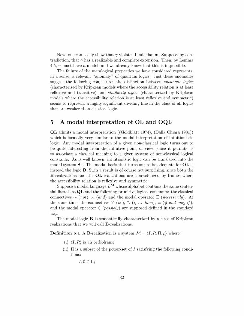
Definition 7.1 Elementary class.

(i) Let Γ be a class of frames. A possible property P of the elements of Γis called first-order (or elementary) iff there exists a sentence η of L2

such that for any 〈I,R〉 ∈ Γ:

〈I,R〉 |= η iff 〈I,R〉 has the property P .

(ii) Γ is said to be an elementary class iff the property of being in Γ is anelementary property of Γ.

Thus, Γ is an elementary class iff there is a sentence η of L2 such that

Γ = 〈I,R〉 | 〈I,R〉 |= η .

Definition 7.2 Elementary substructure.Let 〈I1, R1〉 , 〈I2, R2〉 be two frames.

(a) 〈I1, R1〉 is a substructure of 〈I2, R2〉 iff the following conditions aresatisfied:

(i) I1 ⊆ I2;

(ii) R1 = R2 ∩ (I1 × I1);

(b) 〈I1, R1〉 is an elementary substructure of 〈I2, R2〉 iff the following con-ditions hold:

(i) 〈I1, R1〉 is a substructure of 〈I2, R2〉;

(ii) For any formula α(x1, . . . , xn) of L2 and any i1, . . . , in of I1:

〈I1, R1〉 |= α[i1, . . . in] iff 〈I2, R2〉 |= α[i1, . . . in].

In other words, the elements of the “smaller” structure satisfy exactly thesame L2-formulas in both structures. The following Theorem ((Bell andSlomson 1969))provides an useful criterion to check whether a substructureis an elementary substructure.

Theorem 7.1 Let 〈I1, R1〉 be a substructure of 〈I2, R2〉. Then, 〈I1, R1〉is an elementary substructure of 〈I2, R2〉 iff whenever α(x1, · · · , xn, y) is aformula of L2 (in the free variables x1, · · · , xn, y) and i1, · · · , in are elementsof I1 such that for some j ∈ I2, 〈I2, R2〉 |= α[i1, · · · , in, j], then there is somei ∈ I1 such that 〈I2, R2〉 |= α[i1, · · · , in, i].

42

Let us now consider a pre-Hilbert space 5 H and let H+ := ψ ∈ H | ψ 6= 0,where 0 is the null vector. The pair

⟨

H+,⊥/⟩

is an orthoframe, where ∀ψ, φ ∈ H+: ψ ⊥/ φ iff the inner product of ψand φ is different from the null vector 0 (i.e., (ψ, φ) 6= 0). Let Π(H) be theortholattice of all propositions of 〈H+,⊥/ 〉, which turns out to be isomorphicto the ortholattice C(H) of all (not necessarily closed) subspaces of H (aproposition is simply a subspace devoided of the null vector). The followingdeep Theorem, due to Amemiya and Halperin (Varadarajan 1985) permitsus to characterize the class of all Hilbert spaces in the larger class of allpre-Hilbert spaces, by means of the orthomodular property.

Theorem 7.2 Amemiya-Halperin Theorem.C(H) is orthomodular iff H is a Hilbert space.

In other words, C(H) is orthomodular iff H is metrically complete.As is well known (Bell and Slomson 1969), the property of “being metri-

cally complete” is not elementary. On this basis, it will be highly expectedthat also the orthomodular property is not elementary. The key-lemma inGoldblatt’s proof is the following:

Lemma 7.1 Let Y be an infinite-dimensional (not necessarily closed) sub-space of a separable Hilbert space H. If α is any formula of L2 and ψ1, · · · , ψn

are vectors of Y such that for some φ ∈ H, 〈H+,⊥/ 〉 |= α[ψ1, · · · , ψn, φ], thenthere is a vector ψ ∈ Y such that 〈H+,⊥/ 〉 |= α[ψ1, · · · , ψn, ψ].

As a consequence one obtains:

Theorem 7.3 The orthomodular property is not elementary.

Proof. Let H be any metrically incomplete pre-Hilbert space. Let H be itsmetric completion. Thus H is an infinite-dimensional subspace of the Hilbertspace H. By Lemma 7.1 and by Theorem 7.1, 〈H+,⊥/ 〉 is an elementary sub-

structure of⟨

H+,⊥/

⟩

. At the same time, by Amemiya-Halperin’s Theorem,

C(H) cannot be orthomodular, because H is metrically incomplete. How-ever, C(H) is orthomodular. As a consequence, orthomodularity cannot beexpressed as an elementary property.

5A pre-Hilbert space is a vector space over a division ring whose elements are the realor the complex or the quaternionic numbers such that an inner product (which transformsany pair of vectors into an element of the ring) is defined. Differently from Hilbert spaces,pre-Hilbert spaces need not be metrically complete.

43

The embeddability problem

As we have seen in Section 2, the class of all propositions of an or-thoframe is a complete ortholattice. Conversely, the representation theoremfor ortholattices states that every ortholattice B = 〈B,⊑ , ′ ,1 ,0〉 is embed-dable into the complete ortholattice of all propositions of the orthoframe〈B+,⊥/ 〉, where: B+ := B − 0 and ∀a, b ∈ B: a ⊥/ b iff a 6⊑ b′. Theembedding is given by the map

h : a 7→ 〈a ],

where 〈a ] is the quasi-ideal generated by a. In other words: 〈a ] = b 6= 0 | b ⊑ a.One can prove the following Theorem:

Theorem 7.4 Let B = 〈B,⊑ , ′ ,1 ,0〉 be an ortholattice. ∀X ⊆ B, X is aproposition of 〈B+,⊥/ 〉 iff X = l(u(X)), where:

u(Y ) :=

b ∈ B+ | ∀a ∈ Y : a ⊑ b

and l(Y ) :=

b ∈ B+ | ∀a ∈ Y : b ⊑ a

.

Accordingly, the complete ortholattice of all propositions of the orthoframe〈B+,⊥/ 〉 is isomorphic to the MacNeille completion (or completion by cuts)of B (Kalmbach 1983). 6 At the same time, orthomodularity (similarly todistributivity and modularity) is not preserved by the MacNeille completion,as the following example shows (Kalmbach 1983).

Let C0(2)(IR) be the class of all continuous complex-valued functions f on

IR such that∫ +∞

−∞

| f(x) |2 dx <∞

Let us define the following bilinear form (. , .) : C0(2)(IR) × C0

(2)(IR) → |C

(representing an inner product):

(f, g) =

∫ +∞

−∞

f∗(x)g(x)dx,

where f∗(x) is the complex conjugate of f(x). It turns out that C0(2)(IR),

equipped with the inner product (. , .), gives rise to a metrically incompleteinfinite-dimensional pre-Hilbert space. Thus, by Amemiya-Halperin’s The-orem (Theorem 7.2), the algebraically complete ortholattice C(C0

(2)(IR)) of

6The Mac Neille completion of an ortholattice B = 〈B,⊑ , ′ ,1 ,0〉 is the latticewhose support consists of all X ⊆ B such that X = l(u(X)), where: u(Y ) :=b ∈ B | ∀a ∈ Y : a ⊑ b and l(Y ) := b ∈ B | ∀a ∈ Y : b ⊑ a. Clearly the only differ-ence between the proposition-lattice of the frame

⟨

B+,⊥/⟩

and the Mac Neille completionof B is due to the fact that propositions do not contain 0.

44

all subspaces of C0(2)(IR) cannot be orthomodular. Now consider the sub-

lattice FI of C(C0(2)(IR)), consisting of all finite or cofinite dimensional sub-

spaces. It is not hard to see that FI is orthomodular. One can prove thatC(C0

(2)(IR)) is sup-dense in FI; in other words, any X ∈ C(C0(2)(IR)) is the

sup of a set of elements of FI. Thus, by a theorem proved by McLaren(Kalmbach 1983), the MacNeille completion of C(C0

(2)(IR)) is isomorphic to

the MacNeille completion of FI. Since C(C0(2)(IR)) is algebraically complete,

the MacNeille completion of C(C0(2)(IR)) is isomorphic to C(C0

(2)(IR)) itself.As a consequence, FI is orthomodular, while its MacNeille completion isnot.

8 Hilbert quantum logic and the orthomodular

law

As we have seen, the prototypical models of OQL that are interesting fromthe physical point of view are based on the class H of all Hilbert lattices,whose support is the set C(H) of all closed subspaces of a Hilbert spaceH. Let us call Hilbert quantum logic (HQL) the logic that is semanticallycharacterized by H. A question naturally arises: do OQL and HQL repre-sent one and the same logic? As proved by Greechie (1981) 7, this questionhas a negative answer: there is a lattice-theoretical equation (the so-calledorthoarguesian law) that holds in H, but fails in a particular orthomodu-lar lattice. As a consequence, OQL does not represent a faithful logicalabstraction from its quantum theoretical origin.

Definition 8.1 Let Γ be a class of orthomodular lattices. We say thatOQL is characterized by Γ iff for any T and any α the following conditionis satisfied:

T |=OQLα iff for any B ∈ Γ and any A = 〈B, v〉 : T |=A α.

In order to formulate the orthoarguesian law in an equational way, letus first introduce the notion of Sasaki projection.

Definition 8.2 The Sasaki projection.Let B be an orthomodular lattice and let a, b be any two elements of B. TheSasaki projection of a onto b, denoted by a ⋓ b, is defined as follows:

a ⋓ b := (a ⊔ b′) ⊓ b.

7See also Kalmbach (1983).

45

a

b??

????

??

c??

????

??d

e

Figure 3: The Greechie diagram of G12

It is easy to see that two elements a, b of an orthomodular lattice arecompatible (a = (a ⊓ b′) ⊔ (a ⊓ b)) iff a ⋓ b = a ⊓ b. Consequently, in anyBoolean lattice, ⋓ coincides with ⊓.

Definition 8.3 The orthoarguesian law.

a ⊑ b ⊔

(a ⋓ b′) ⊓ [(a ⋓ c′) ⊔ ((b ⊔ c) ⊓ ((a ⋓ b′) ⊔ (a ⋓ c′)))]

(OAL)

Greechie has proved that (OAL) holds in H but fails in a particular finiteorthomodular lattice. In order to understand Greechie’s counterexample, itwill be expedient to illustrate the notion of Greechie diagram.

Let us first recall the definition of atom.

Definition 8.4 Atom.Let B = 〈B,⊑,1,0〉 any bounded lattice. An atom is an element a ∈ B−0such that:

∀b ∈ B : 0 ⊑ b ⊑ a y b = 0 or a = b.

Greechie diagrams are hypergraphs that permits us to represent partic-ular orthomodular lattices. The representation is essentially based on thefact that a finite Boolean algebra is completely determined by its atoms. AGreechie diagram of an orthomodular lattice B consists of points and lines.Points are in one-to-one correspondence with the atoms of B; lines are inone-to-one correspondence with the maximal Boolean subalgebras 8 of B.Two lines are crossing in a common atom. For example, the Greechie dia-gram pictured in Figure 3. represents the orthomodular lattice G12 (Figure4).

Let us now consider a particular finite orthomodular lattice, called B30,whose Greechie diagram is pictured in Figure 3.

8A maximal Boolean subalgebra of an ortholattice B is a Boolean subalgebra of B, thatis not a proper subalgebra of any Boolean subalgebra of B.

46

•1

•a′oooooooooooooo

•a

OOOOOOOOOOOOOOO •b??

????

??

????

????

•cOOOOOOOOOOOOOO

•0

•b′

•−

????

????

•c′

ooooooooooooooo

•d??

????

??

•eOOOOOOOOOOOOOO •d′

????

????

????

????

ooooooooooooooo

•e′OOOOOOOOOOOOOO

ooooooooooooooo

Figure 4: The orthomodular lattice G12

a

o

n

c

i

h

g

f

????

????

e??

????

?? b

m

????????

l

????????

k

s

r????????

????????

Figure 5: The Greechie diagram of B30

47

Theorem 8.1 (OAL) fails in B30.

Proof. There holds: a ⋓ b′ = (a ⊔ b) ⊓ b′ = s′ ⊓ b′ = e, a ⋓ c′ = (a ⊔ c) ⊓ c′ =n′ ⊓ c′ = i and b ⊔ c = l′. Thus,

b ⊔ (a ⋓ b′) ⊓ [(a ⋓ c′) ⊔ ((b ⊔ c) ⊓ ((a ⋓ b′) ⊔ (a ⋓ c′)))]

= b ⊔

e ⊓[

i ⊔ (l′ ⊓ (e ⊔ i))]

= b ⊔

e ⊓[

i ⊔ (l′ ⊓ g′)]

= b ⊔ (e ⊓ (i ⊔ 0))

= b ⊔ (e ⊓ i)

= b

6⊒ a.

Hence, there are two formulas α and β (whose valuations in a convenientrealization represent the left- and right- hand side of (OAL), respectively)such that α |=

OQL/ β. At the same time, for any C(H) ∈ H and for any

realization A = 〈C(H), v〉, there holds: α |=A β.As a consequence, OQL is not characterized by H. Accordingly, HQL

is definitely stronger than OQL. We are faced with the problem of findingout a calculus, if any, that turns out to be sound and complete with respectto H. The main question is whether the class of all formulas valid in H isrecursively enumerable. In order to solve this problem, it would be sufficient(but not necessary) to show that the canonical model of HQL is isomorphicto the subdirect product of a class of Hilbert lattices. So far, very little isknown about this question.

Lattice characterization of Hilbert lattices

As mentioned in the Introduction, the algebraic structure of the set E of theevents in an event-state system 〈E , S〉 is usually assumed to be a σ-completeorthomodular lattice. Hilbert lattices, however, satisfy further importantstructural properties. It will be expedient to recall first some standardlattice theoretical definitions. Let B = 〈B,⊑,1,0〉 be any bounded lattice.

Definition 8.5 Atomicity .A bounded lattice B is atomic iff ∀a ∈ B − 0 there exists an atom b suchthat b ⊑ a.

48

Definition 8.6 Covering property .Let a, b be two elements of a lattice B. We say that b covers a iff a ⊑ b , a 6= b,and ∀c ∈ B : a ⊑ c ⊑ b y a = c or b = c.A lattice B satisfies the covering property iff ∀a, b ∈ B: a covers a ⊓ b y

a ⊔ b covers b.

Definition 8.7 Irreducibility .Let B be an orthomodular lattice. B is said to be irreducible iff

a ∈ B | ∀b ∈ B : a is compatible with b = 0,1.

One can prove the following theorem:

Theorem 8.2 Any Hilbert lattice is a complete, irreducible, atomic ortho-modular lattice, which satisfies the covering property.

Are these conditions sufficient for a lattice B to be isomorphic to (orembeddable into) a Hilbert lattice? In other words, is it possible to capturelattice-theoretically the structure of Hilbert lattices? An important resultalong these lines is represented by the so-called Piron-McLaren’s coordina-tization theorem (Varadarajan 1985).

Theorem 8.3 Piron-McLaren coordinatization theorem.Any lattice B (of length 9 at least 4) that is complete, irreducible, atomicwith the covering property, is isomorphic to the orthomodular lattice of all(. , .)-closed subspaces of a Hilbertian space 〈V, θ, (. , .),D〉. 10

Do the properties of the coordinatized lattice B restrict the choice to oneof the real, the complex or the quaternionic numbers ( |Q) and thereforeto a classical Hilbert space? Quite unexpectedly, Keller (1980) proved anegative result: there are lattices that satisfy all the conditions of Piron-McLaren’s Theorem; at the same time, they are coordinatized by Hilbertianspaces over non-archimedean division rings. Keller’s counterexamples havebeen interpreted by some authors as showing the definitive impossibility for

9 The length of a lattice B is the supremum over the numbers of elements of all thechains of B, minus 1.

10 A Hilbertian space is a 4-tuple 〈V, θ, (. , .),D〉, where V is a vector space over adivision ring D, θ is an involutive antiautomorphism on D, and (. , .) (to be interpretedas an inner product) is a definite symmetric θ-bilinear form on V. Let X be any subset ofV and let X ′ := ψ ∈ V | ∀φ ∈ X, (ψ, φ) = 0; X is called (. , .)-closed iff X = X ′′.If D is either IR or |C or |Q and the antiautomorphism θ is continuous, then 〈V, θ, (. , .),D〉turns out to be a classical Hilbert space.

49

the quantum logical approach to capture the Hilbert space mathematics.This impossibility was supposed to demonstrate the failure of the quantumlogic approach in reaching its main goal: the “bottom-top” reconstruction ofHilbert lattices. Interestingly enough, such a negative conclusion has beenrecently contradicted by an important result proved by Soler (Soler 1995):Hilbert lattices can be characterized in a lattice-theoretical way. Soler resultis essentially based on the following Theorem:

Theorem 8.4 Let 〈V, θ, (. , .),D〉 be an infinite-dimensional Hilbertian spaceover a division ring D. Suppose our space includes a k-orthogonal setψii∈IN, i.e., a family of vectors of V such that ∀i : (ψi, ψi) = k and∀i, j(i 6= j) : (ψi, ψj) = 0. Then D is either IR or |C or |Q. Therefore〈V, θ, (. , .),D〉 is a classical Hilbert space.

As a consequence, the existence of k-orthogonal sets characterizes Hilbertspaces in the class of all Hilbertian spaces. The point is that the existenceof such sets admits of a purely lattice-theoretic characterization, by meansof the so-called angle bisecting condition (Morash 1973). Accordingly, everylattice which satisfies the angle bisecting condition (in addition to the usualconditions of Piron-McLaren’s Theorem) is isomorphic to a classical Hilbertlattice.

Soler’s Theorem is a purely mathematical result and a plausible phys-ical interpretation of the angle bisecting condition is presently beyond theresearch horizon.

9 First-order quantum logic

The most significant logical and metalogical peculiarities of QL arise at thesentential level. At the same time the extension of sentential QL to a first-order logic seems to be quite natural. Similarly to the case of sententialQL, we will characterize first-order QL both by means of an algebraic anda Kripkean semantics.

Suppose a standard first-order language with predicates Pnm and individ-

ual constants am.11 The primitive logical constants are the connectives ¬,∧and the universal quantifier ∀. The concepts of term, formula and sentenceare defined in the usual way. We will use x, y, z, x1, · · · , xn, · · · as metavari-ables ranging over the individual variables, and t, t1, t2, · · · as metavariables

11For the sake of simplicity, we do not assume functional symbols.

50

ranging over terms. The existential quantifier ∃ is supposed defined by ageneralized de Morgan law:

∃xα := ¬∀x¬α.

Definition 9.1 Algebraic realization for first-order OL.An algebraic realization for (first-order) OL is a system A =

⟨

BC ,D , v⟩

where:

(i) BC =⟨

BC ,⊑ , ′ ,1 ,0⟩

is an ortholattice closed under infinitaryinfimum (

⊔

) and supremum (⊔

) for any F ⊆ BC such that F ∈ C(C being a particular family of subsets of BC).

(ii) D is a non-empty set (disjoint from B) called the domain of A.

(iii) v is the valuation-function satisfying the following conditions:

• for any constant am: v(am) ∈ D; for any predicate Pnm, v(Pn

n )is an n-ary attribute in A, i.e., a function that associates toany n-tuple 〈d1, · · · ,dn〉 of elements of D an element (truth-value) of B;

• for any interpretation σ of the variables in the domain D (i.e.,for any function from the set of all variables into D) the pair〈v, σ〉 (abbreviated by vσ and called generalized valuation)associates to any term an element in D and to any formulaa truth-value in B, according to the conditions:

vσ(am) = v(am)

vσ(x) = σ(x)

vσ(Pnmt1, · · · , tn) = v(Pn

m)(vσ(t1), · · · , vσ(tn))

vσ(¬β) = vσ(β)′

vσ(β ∧ γ) = vσ(β) ⊓ vσ(γ)

vσ(∀xβ) =

⊔

vσ[x/d](β) | d ∈ D

, where

vσ[x/d](β) | d ∈ D

∈C

(σ[x/d] is the interpretation that associates to x the individuald and differs from σ at most in the value attributed to x).

Definition 9.2 Truth and logical truth.A formula α is true in A =

⟨

BC ,D, v⟩

(abbreviated as |=A α) iff for anyinterpretation of the variables σ, vσ(α) = 1;α is a logical truth of OL (|=

OLα) iff for any A, |=A α

51

Definition 9.3 Consequence in a realization and logical consequence.Let A =

⟨

BC ,D, v⟩

be a realization. A formula α is a consequence of T inA (abbreviated T |=A α ) iff for any element a of B and any interpretationσ: if for any β ∈ T , a ⊑ vσ(β), then a ⊑ vσ(α);α is a logical consequence of T (T |=

OLα ) iff for any realization A: T |=A α.

Definition 9.4 Kripkean realization for (first-order) OL.A Kripkean realization for (first-order) OL is a system K =

⟨

I ,R ,ΠC , U , ρ⟩

where:

(i)⟨

I ,R ,ΠC⟩

satisfies the same conditions as in the sentential case;further ΠC is closed under infinitary intersection for any F ⊆ Πsuch that F ∈ C (where C is a particular family of subsets ofΠC);

(ii) U , called the domain of K, is a non-empty set, disjoint from theset of worlds I. The elements of U are individual concepts u suchthat for any world i: u(i) is an individual (called the reference ofu in the world i). An individual concept u is called rigid iff for anypairs of worlds i, j: u(i) = u(j). The set Ui = u(i) | u ∈ Urepresents the domain of individuals in the world i . WheneverUi = Uj for all i,j we will say that the realization K has a constantdomain.

(iii) ρ associates a meaning to any individual constant am and to anypredicate Pn

m according to the following conditions:

ρ(am) is an individual concept in U .

ρ(Pnm) is a predicate-concept , i.e. a function that associates to

any n-tuple of individual concepts 〈u1, · · · ,un〉 a propositionin ΠC ;

(iv) for any interpretation of the variables σ in the domain U , thepair 〈ρ , σ〉 (abbreviated as ρσ and called valuation) associatesto any term t an individual concept in U and to any formula aproposition in ΠC according to the conditions:

ρσ(x) = σ(x)

ρσ(am) = ρ(am)

ρσ(Pnmt1, · · · , tn) = ρ(Pn

m)(ρσ(t1), · · · , ρσ(tn))

ρσ(¬β) = ρσ(β)′

ρσ(β ∧ γ) = ρσ(β) ∩ ρσ(γ)

52

ρσ(∀xβ) =⋂

ρσ[x/u](β) | u ∈ U

, where

ρσ[x/u](β) | u ∈ U

∈C.

For any world i and any interpretation σ of the variables, the triplet 〈ρ , i , σ〉(abbreviated as ρσ

i ) will be called a world-valuation.

Definition 9.5 Satisfaction.ρσ

i |= α (ρσi satisfies α) iff i ∈ ρσ(α).

Definition 9.6 Verification.ρσ

i |= α (i verifies α) iff for any σ: ρσi |= α.

Definition 9.7 Truth and logical truth.|=K α (α is true in K) iff for any i: i |= α;|=

OLα (α is a logical truth of OL) iff for any K: |=K α.

Definition 9.8 Consequence in a realization and logical consequence.T |=K α iff for any i of K and any σ: ρσ

i |= T y ρσi |= α;

T |=OLα iff for any realization K: T |=K α.

The algebraic and the Kripkean characterization for first-order OQL

can be obtained, in the obvious way, by requiring that any realization beorthomodular.

In both semantics for first-order QL one can prove a coincidence lemma:

Lemma 9.1 Given A =⟨

BC ,D , v⟩

and K =⟨

I ,R ,ΠC , U, ρ⟩

:

(9.1.1) If σ and σ∗ coincide in the values attributed to the variables oc-curring in a term t, then vσ(t) = vσ∗

(t); ρσ(t) = ρσ∗(t).

(9.1.2) If σ and σ∗ coincide in the values attributed to the free variablesoccurring in a formula α, then vσ(α) = vσ∗

(α); ρσ(α) = ρσ∗(α).

One can easily prove, like in the sentential case, the following lemma:

Lemma 9.2

(9.2.1) For any algebraic realization A there exists a Kripkean realizationKA such that for any α: |=A α iff |=KA α. Further, if A isorthomodular then KA is orthomodular.

53

(9.2.2) For any Kripkean realization K, there exists an algebraic realiza-tion AK such that for any for any α: |=K α iff |=AK α. Further,if K is orthomodular then AK is orthomodular.

An axiomatization of first-order OL (OQL) can be obtained by addingto the rules of our OL (OQL)-sentential calculus the following new rules:

(PR1) T ∪ ∀xα |−α(x/t), where α(x/t) indicates a legitimate sub-stitution).

(PR2)T |−α

T |− ∀xα(provided x is not free in T ).

All the basic syntactical notions are defined like in the sentential case.One can prove that any consistent set of sentences T admits of a consistentinductive extension T ∗, such that T ∗ |− ∀xα(t) whenever for any closed termt, T ∗ |−α(t). The “weak Lindenbaum theorem” can be strengthened asfollows: if T |−/¬α then there exists a consistent and inductive T ∗ such that:

T is syntactically compatible with T ∗ and T ∗ |−α.12

One can prove a soundness and a completeness theorem of our calculuswith respect to the Kripkean semantics.

Theorem 9.1 Soundness.T |−α y T |= α.

Proof. Straightforward.

Theorem 9.2 Completeness.T |= α y T |−α.

Sketch of the proof. Like in the sentential case, it is sufficient to constructa canonical model K =

⟨

I ,R ,ΠC , U , ρ⟩

such that T |−α iff T |=K α.

Definition of the canonical model

(i) I is the set of all consistent, deductively closed and inductive sets ofsentences expressed in a common language LK , which is an extensionof the original language;

12By Definition 6.6, T is syntactically compatible with T ∗ iff there is no formula α suchthat T |−α and T ∗ |− ¬α.

54

(ii) R is determined like in the sentential case;

(iii) U is a set of rigid individual concepts that is naturally determined bythe set of all individual constants of the extended language LK. Forany constant c of LK, let uc be the corresponding individual conceptin U . We require: for any world i, uc(i) = c. In other words, thereference of the individual concept uc is in any world the constant c.We will indicate by cu the constant corresponding to u.

(iv) ρ(am) = uam ;

ρ(Pnm)(uc1

1 , . . . ,ucnn ) = i | Pn

mc1, . . . , cn ∈ i .

Our ρ is well defined since one can prove for any sentence α of LK:

i |−/α y ∃j ⊥/ i : j |−¬α.

As a consequence, ρσ(Pnmt1, . . . , tn) is a possible proposition.

(v) ΠC is the set of all “meanings” of formulas (i.e., X ∈ ΠC iff ∃α∃σ(X =ρσ(α)); C is the set of all sets

ρσ[x/u](β) | u ∈ U

for any formula β.

One can easily check that K is a “good” realization with a constantdomain.

Lemma 9.3 Lemma of the canonical model.For any α, any i ∈ I and any σ:

ρσi |= α iff ασ ∈ i,

where ασ is the sentence obtained by substituting in α any free variable xwith the constant cσ(x) corresponding to the individual concept σ(x).

Sketch of the proof. By induction on the length of α. The cases α =Pn

mt1, · · · , tn, α = ¬β, α = β ∧ γ are proved by an obvious transformationof the sentential argument. Let us consider the case α = ∀xβ and supposex occurring in β (otherwise the proof is trivial). In order to prove the leftto right implication, suppose ρσ

i |= ∀xβ. Then, for any u in U , ρσ[x/u] |=β(x). Hence, by inductive hypothesis, ∀u ∈ U , [β(x)]σ[x/u] ∈ i. In otherwords, for any constant cu of i: [β(x)]σ(x/cu) ∈ i. And, since i is inductiveand deductively closed: ∀xβ(x)σ ∈ i. In order to prove the right to leftimplication, suppose [∀xβ(x)]σ ∈ i. Then, [by (PR1)], for any constant c of

i: [β(x/c)]σ ∈ i. Hence by inductive hypothesis: for any uc ∈ U , ρσ[x/uc]i |=

β(x), i.e., ρσi |= ∀xβ(x). On this ground, similarly to the sentential case,

one can prove T |−α iff T |=K α.

55

First-order QL can be easily extended (in a standard way) to a first-order logic with identity. However, a critical problem is represented by thepossibility of developing, within this logic, a satisfactory theory of descrip-tions. The main difficulty can be sketched as follows. A natural condition tobe required in any characterization of a ι-operator is obviously the following:

∃x β(x) ∧ ∀y [(β(y) ∧ x = y) ∨ (¬β(y) ∧ ¬x = y)] ∧ α(x)

is true y α(ιxβ(x)) is true.

However, in QL, the truth of the antecedent of our implication does notgenerally guarantee the existence of a particular individual such that ιxβ canbe regarded as a name for such an individual. As a counterexample, let usconsider the following case (in the algebraic semantics): let A be 〈B ,D , v〉where B is the complete orthomodular lattice based on the set of all closedsubspaces of the plane IR2, and D contains exactly two individuals d1,d2.Let P be a monadic predicate and X,Y two orthogonal unidimensionalsubspaces of B such that v(P )(d1) = X, v(P )(d2) = Y . If the equalitypredicate = is interpreted as the standard identity relation (i.e., vσ(t1 =t2) = 1, if vσ(t1) = vσ(t2); 0, otherwise), one can easily calculate:

v (∃x [Px ∧ ∀y((Py ∧ x = y) ∨ (¬Py ∧ ¬x = y))]) = 1.

However, for both individuals d1,d2 of the domain, we have:

vσ[x/d1](Px) 6= 1, vσ[x/d2](Px) 6= 1.

In other words, there is no precise individual in the domain that satisfiesthe property expressed by predicate P !

10 Quantum set theories and theories of quasisets

An important application of QL to set theory has been developed by Takeuti(1981). We will sketch here only the fundamental idea of this application.Let L be a standard set-theoretical language. One can construct ortho-valued models for L, which are formally very similar to the usual Boolean-valued models for standard set-theory, with the following difference: the setof truth-values is supposed to have the algebraic structure of a completeorthomodular lattice, instead of a complete Boolean algebra. Let B be acomplete orthomodular lattice, and let ν, λ,... represent ordinal numbers.An ortho-valued (set-theoretical) universe V is constructed as follows:

56

V B =⋃

ν∈On V (ν) , where:

V (0) = ∅.

V (ν+1) = g | g is a function andDom(g) ⊆ V (ν) andRang(g) ⊆ B.

V (λ) =⋃

ν<λ V (ν), for any limit-ordinal λ.

( Dom(g) and Rang(g) are the domain and the range of functiong, respectively).

Given an orthovalued universe V B one can define for any formula of L thetruth-value [[α]]σ in B induced by any interpretation σ of the variables intothe universe V B.

[[x ∈ y]]σ =⊔

g∈Dom(σ(y))

σ(y)(g) ⊓ [[x = z]]σ[z/g]

[[x = y]]σ =

⊔g∈Dom(σ(x))

σ(x)(g) [[z ∈ y]]σ[z/g]

⊓

⊔g∈Dom(σ(y))

σ(y)(g) [[z ∈ x]]σ[z/g]

.

where is the quantum logical conditional operation (a b := a′⊔ (a⊓ b),for any a, b ∈ B).

A formula α is called true in the universe V B (|=V B α) iff [[α]]σ = 1, forany σ.

Interestingly enough, the segment V (ω) of V B turns out to contain someimportant mathematical objects, that we can call quantum-logical naturalnumbers.

The standard axioms of set-theory hold in B only in a restricted form.An extremely interesting property of V B is connected with the notion ofidentity. Differently from the case of Boolean-valued models, the identityrelation in V B turns out to be non-Leibnizian. For, one can choose anorthomodular lattice B such that:

6|=V B x = y → ∀z(x ∈ z ↔ y ∈ z).

According to our semantic definitions, the relation = represents a kindof “extensional equality”. As a consequence, one may conclude that twoquantum-sets that are extensionally equal do not necessarily share all thesame properties. Such a failure of the Leibniz-substitutivity principle inquantum set theory might perhaps find interesting applications in the fieldof intensional logics.

A completely different approach is followed in the framework of the the-ories of quasisets (or quasets). The basic aim of these theories is to providea mathematical description for collections of microobjects, which seem toviolate some characteristic properties of the classical identity relation.

57

In some of his general writings, Schrodinger discussed the inconsistencybetween the classical concept of physical object (conceived as an individualentity) and the behaviour of particles in quantum mechanics. Quantumparticles – he noticed – lack individuality and the concept of identity cannotbe applied to them, similarly to the case of classical objects.

One of the aims of the theories of quasisets (proposed by da Costa,French and Krause (1992)) is to describe formally the following idea de-fended by Schrodinger: identity is generally not defined for microobjects.As a consequence, one cannot even assert that an “electron is identical withitself”. In the realm of microobjects only an indistinguishability relation(an equivalence relation that may violate the substitutivity principle) makessense.

On this basis, different formal systems have been proposed. Generally,these systems represent convenient generalizations of a Zermelo-Fraenkel likeset theory with urelements. Differently from the classical case, an urelementmay be either a macro or a micro object . Collections are represented byquasisets and classical sets turn out to be limit cases of quasisets.

A somewhat different approach has been followed in the theory of quasets(proposed in (Dalla Chiara and Toraldo di Francia 1993)).

The starting point is based on the following observation: physical kindsand compound systems in QM seem to share some features that are charac-teristic of intensional entities. Further, the relation between intensions andextensions turns out to behave quite differently from the classical semanticsituations. Generally, one cannot say that a quantum intensional notionuniquely determines a corresponding extension. For instance, take the no-tion of electron, whose intension is well defined by the following physicalproperty: mass = 9.1 × 10−28g, electron charge = 4.8 × 10−10e.s.u., spin= 1/2. Does this property determine a corresponding set , whose elementsshould be all and only the physical objects that satisfy our property at acertain time interval? The answer is negative. In fact, physicists have thepossibility of recognizing, by theoretical or experimental means, whether agiven physical system is an electron system or not. If yes, they can alsoenumerate all the quantum states available within it. But they can do soin a number of different ways. For example, take the spin. One can choosethe x-axis and state how many electrons have spin up and how many havespin down. However, we could instead refer to the z-axis or any other direc-tion, obtaining different collections of quantum states, all having the samecardinality. This seems to suggest that microobject systems present an ir-reducibly intensional behaviour: generally they do not determine preciseextensions and are not determined thereby. Accordingly, a basic feature of

58

the theory is a strong violation of the extensionality principle.Quasets are convenient generalizations of classical sets, where both the

extensionality axiom and Leibniz’ principle of indiscernibles are violated.Generally a quaset has only a cardinal but not an ordinal number, since itcannot be well ordered.

11 The unsharp approaches

The unsharp approaches to QT (first proposed by Ludwig (1983) and furtherdeveloped by Kraus, Davies, Mittelstaedt, Busch, Lahti, Bugajski, Beltram-etti, Cattaneo and many others) have been suggested by some deep criticismof the standard logico-algebraic approach. Orthodox quantum logic (basedon Birkhoff and von Neumann’s proposal) turns out to be at the same timea total and a sharp logic. It is total because the meaningful propositionsare represented as closed under the basic logical operations: the conjunction(disjunction) of two meaningful propositions is a meaningful proposition.Further, it is also sharp, because propositions, in the standard interpreta-tion, correspond to exact possible properties of the physical system underinvestigation. These properties express the fact that “the value of a givenobservable lies in a certain exact Borel set”.

As we have seen, the set of the physical properties, that may hold fora quantum system, is mathematically represented by the set of all closedsubspaces of the Hilbert space associated to our system. Instead of closedsubspaces, one can equivalently refer to the set of all projections, that is inone-to-one correspondence with the set of all closed subspaces. Such a cor-respondence leads to a collapse of different semantic notions, which Foulisand Randall described as the “metaphysical disaster” of orthodox QT. Thecollapse involves the notions of “experimental proposition”, “physical prop-erty”, “physical event” (which represent empirical and intensional con-cepts), and the notion of proposition as a set of states (which correspondsto a typical extensional notion according to the tradition of standard se-mantics).

Both the total and the sharp character of QL have been put in questionin different contexts. One of the basic ideas of the unsharp approaches is a“liberalization” of the mathematical counterpart for the intuitive notion of“experimental proposition”. Let P be a projection operator in the Hilbertspace H, associated to the physical system under investigation. Suppose Pdescribes an experimental proposition and let W be a statistical operatorrepresenting a possible state of our system. Then, according to one of the

59

axioms of the theory (the Born rule), the number Tr(WP ) (the trace ofthe operator WP ) will represent the probability-value that our system instate W verifies P . This value is also called Born probability . However,projections are not the only operators for which a Born probability can bedefined. Let us consider the class E(H) of all linear bounded operators Esuch that for any statistical operator W ,

Tr(WE) ∈ [0, 1].

It turns out that E(H) properly includes the set P (H) of all projections onH. The elements of E(H) represent, in a sense, a “maximal” mathematicalrepresentative for the notion of experimental proposition, in agreement withthe probabilistic rules of quantum theory. In the framework of the unsharpapproach, E(H) has been called the set of all effects13. An important dif-ference between projections and proper effects is the following: projectionscan be associated to sharp propositions having the form “the value for theobservable A lies in the exact Borel set ∆”, while effects may represent alsofuzzy propositions like “the value of the observable A lies in the fuzzy Borelset Γ”. As a consequence, there are effects E, different from the null pro-jection |O, such that no state W can verify E with probability 1. A limitcase is represented by the semitransparent effect 1

21I (where 1I is the identityoperator), to which any state W assigns probability-value 1

2 .From the intuitive point of view, one could say that moving to an unsharp

approach represents an important step towards a kind of “second degree offuzziness”. In the framework of the sharp approach, any physical event Ecan be regarded as a kind of “clear” property. Whenever a state W assignsto E a probability value different from 1 and 0, one can think that thesemantic uncertainty involved in such a situation totally depends on theambiguity of the state (first degree of fuzziness). In other words, even apure state in QT does not represent a logically complete information, thatis able to decide any possible physical event. In the unsharp approaches,instead, one take into account also “genuine ambiguous properties”. Thissecond degree of fuzziness may be regarded as depending on the accuracyof the measurement (which tests the property), and also on the accuracyinvolved in the operational definition for the physical quantities which ourproperty refers to.

13It is easy to see that an effect E is a projection iff E2 := EE = E. In other words,projections are idempotent effects.

60

12 Effect structures

Different algebraic structures can be induced on the class E(H) of all effects.Let us first recall some definitions.

Definition 12.1 Involutive bounded poset (lattice).An involutive bounded poset (lattice) is a structure B = 〈B ,⊑ , ′ ,1 ,0〉,where 〈B ,⊑ ,1 ,0〉 is a partially ordered set (lattice) with maximum (1) andminimum (0); ′ is a 1-ary operation on B such that the following conditionsare satisfied: (i) a′′ = a; (ii) a ⊑ b y b′ ⊑ a′.

Definition 12.2 Orthoposet.An orthoposet is an involutive bounded poset that satisfies the non contra-diction principle:

a ⊓ a′ = 0.

Definition 12.3 Orthomodular poset.An orthomodular poset is an orthoposet that is closed under the orthogonalsup (a ⊑ b′ y a ⊔ b exists) and satisfies the orthomodular property:

a ⊑ b y ∃c such that a ⊑ c′ and b = a ⊔ c.

Definition 12.4 Regularity.An involutive bounded poset (lattice) B is regular iff a ⊑ a′ and b ⊑ b′ y

a ⊑ b′.

Whenever an involutive bounded poset B is a lattice, then B is regular iff itsatisfies the Kleene condition:

a ⊓ a′ ⊑ b ⊔ b′.

The set E(H) of all effects can be naturally structured as an involutivebounded poset:

E(H) =⟨

E(H) ,⊑ , ′ ,1 ,0⟩

,

where

(i) E ⊑ F iff for any state (statistical operator) W , Tr(WE) ≤ Tr(WE)(in other words, any state assigns to E a probability-value that is lessor equal than the probability-value assigned to F );

61

(ii) 1, 0 are the identity (1I) and the null ( |O) projection, respectively;

(iii) E′ = 1 − E.

One can easily check that ⊑ is a partial order, ′ is an order-reversing invo-lution, while 1 and 0 are respectively the maximum and the minimum withrespect to ⊑. At the same time this poset fails to be a lattice. Differentlyfrom projections, some pairs of effects have no infimum and no supremumas the following example shows (Greechie and Gudder n.d.):

Example 12.1 Let us consider the following effects (in the matrix-representation)on the Hilbert space IR2:

E =

(

12 00 1

2

)

F =

(

34 00 1

4

)

G =

(

12 00 1

4

)

It is not hard to see that G ⊑ E,F . Suppose, by contradiction, that L =E ⊓ F exists in E(IR2). An easy computation shows that L must be equalto G. Let

M =

(

716

18

18

316

)

Then M is an effect such that M ⊑ E,F ; however, M 6⊑ L, which is acontradiction.

In order to obtain a lattice structure, one has to embed E(H) into itsMac Neille completion E(H).

The Mac Neille completion of an involutive bounded poset

Let 〈B ,⊑ ,1 ,0〉 be an involutive bounded poset. For any non-emptysubset X of B, let l(X) and u(X) represent respectively the set of alllower bounds and the set of all upper bounds of X. Let MC(B) :=X ⊆ B | X = u(l(X)). It turns out that X ∈ MC(B) iff X = X ′′,where X ′ := a ∈ B | ∀b ∈ X : a ⊑ b′. Moreover, the structure

B =⟨

MC(B) ,⊆ ,′ , 0 , B⟩

is a complete involutive bounded lattice (which is regular if B is regu-lar), where X ⊓ Y = X ∩ Y and X ⊔ Y = (X ∪ Y )′′.

It turns out that B is embeddable into B, via the map h : a → 〈a],where 〈a] is the principal ideal generated by a. Such an embeddingpreserves the infimum and the supremum, when existing in B.

62

The Mac Neille completion of an involutive bounded poset does notgenerally satisfies the non contradiction principle (a ⊓ a′ = 0 ) and the ex-cluded middle principle (a⊔a′ = 1 ). As a consequence, differently from theprojection case, the Mac Neille completion of E(H) is not an ortholattice.Apparently, our operation ′ turns out to behave as a fuzzy negation, bothin the case of E(H) and of its Mac Neille completion. This is one of thereasons why proper effects (that are not projections) may be regarded asrepresenting unsharp physical properties, possibly violating the non contra-diction principle.

The effect poset E(H) can be naturally extended to a richer structure,equipped with a new complement ∼, that has an intuitionistic-like behaviour:

E∼ is the projection operator PKer(E) whose range is the kernelKer(E)of E, consisting of all vectors that are transformed by the operator Einto the null vector.

By definition, the intuitionistic complement of an effect is always a pro-jection. In the particular case, where E is a projection, it turns out that:E′ = E∼. In other words, the fuzzy and the intuitionistic complementcollapse into one and the same operation.

The structure 〈E(H) ,⊑ , ′ , ∼ ,1 ,0〉 turns out to be a particular exampleof a Brouwer Zadeh poset(Cattaneo and Nistico 1986).

Definition 12.5 A Brouwer Zadeh poset (simply a BZ-poset) is a structure〈B ,⊑ , ′ , ∼ ,1 ,0〉, where

(12.3.1) 〈B ,⊑ , ′ ,1 ,0〉 is a regular involutive bounded poset;

(12.3.2) ∼ is a 1-ary operation on B, which behaves like an intuitionisticcomplement:

(i) a ⊓ a∼ = 0.

(ii) a ⊑ a∼∼.

(iii) a ⊑ b y b∼ ⊑ a∼.

(12.3.3) The following relation connects the fuzzy and the intuitionisticcomplement:

a∼′ = a∼∼.

Definition 12.6 A Brouwer Zadeh lattice is a BZ-poset that is also a lat-tice.

The Mac Neille completion of a BZ-poset

63

Let B = 〈B ,⊑ , ′ , ∼ ,1 ,0〉 be a BZ-poset and let B the Mac Neillecompletion of the regular involutive bounded poset 〈B ,⊑ , ′ , 1 ,0〉.For any non-empty subset X of B, let

X∼ := a ∈ B | ∀b ∈ X : a ⊑ b∼ .

It turns out that B = 〈MC(B),⊆ , ′ , ∼ , 0 , B〉 is a complete BZ-lattice (Giuntini 1991), which B can be embedded into, via the map hdefined above.

Another interesting way of structuring the set of all effects can be ob-tained by using a particular kind of partial structure, that has been called ef-fect algebra (Foulis and Bennett 1994) or unsharp orthoalgebra (Dalla Chiaraand Giuntini (1994)). Abstract effect algebras are defined as follows:

Definition 12.7 An effect algebra is a partial structure A = 〈A ,⊞ ,1 ,0〉where ⊞ is a partial binary operation on A. When ⊞ is defined for a paira , b ∈ A, we will write ∃ (a⊞ b). The following conditions hold:

(i) Weak commutativity

∃(a⊞ b) y ∃(b⊞ a) and a⊞ b = b⊞ a.

(ii) Weak associativity

[∃(b ⊞ c) and ∃(a ⊞ (b ⊞ c))] y [∃(a ⊞ b) and ∃((a ⊞ b) ⊞ c)and a⊞ (b⊞ c) = (a⊞ b)⊞ c].

(iii) Strong excluded middle

For any a, there exists a unique x such that a⊞ x = 1.

(iv) Weak consistency

∃(a⊞ 1) y a = 0.

From an intuitive point of view, our operation ⊞ can be regarded as anexclusive disjunction (aut), which is defined only for pairs of logically in-compatible events.

An orthogonality relation ⊥, a partial order relation ⊑ and a generalizedcomplement ′ can be defined in any effect algebra.

Definition 12.8 Let A = 〈A ,⊞ ,1 ,0〉 be an effect algebra and let a, b ∈ A.

(i) a ⊥ b iff a⊞ b is defined in A.

(ii) a ⊑ b iff ∃c ∈ A such that a ⊥ c and b = a⊞ c.

64

(iii) The generalized complement of a is the unique element a′ suchthat a⊞ a′ = 1 (the definition is justified by the strong excludedmiddle condition).

The category of all effect algebras turns out to be (categorically) equiva-lent to the category of all difference posets, which have been first studied inKopka and Chovanec (1994) and further investigated in Dvurecenskij andPulmannova (1994).

Effect algebras that satisfy the non contradiction principle are calledorthoalgebras:

Definition 12.9 An orthoalgebra is an effect algebra B = 〈B ,⊞ ,1 ,0〉 suchthat the following condition is satisfied:

Strong consistency

∃ (a⊞ a) y a = 0.

In other words: 0 is the only element that is orthogonal to itself.

In order to induce the structure of an effect algebra on E(H), it is suffi-cient to define a partial sum ⊞ as follows:

∃ (E ⊞ F ) iff E + F ∈ E(H),

where + is the usual sum-operator. Further:

∃ (E ⊞ F ) y E ⊞ F = E + F.

It turns out that the structure 〈E(H) ,⊞ , 1I , |O〉 is an effect algebra, wherethe generalized complement of any effect E is just 1I−E. At the same time,this structure fails to be an orthoalgebra.

Any abstract effect algebra

A = 〈A ,⊞ ,1 ,0〉

can be naturally extended to a kind of total structure, that has been termedquantum MV-algebra(abbreviated as QMV-algebra) (Giuntini 1996).

Before introducing QMV-algebras, it will be expedient to recall the def-inition of MV-algebra. As is well known, MV-algebras (multi-valued alge-bras) have been introduced by Chang (Chang 1957) in order to provide analgebraic proof of the completeness theorem for Lukasiewicz ’ infinite-many-valued logic Lℵ. A “privileged” model of this logic is based on the real

65

interval [0, 1], which gives rise to a particular example of a totally ordered(or linear) MV-algebra.

Both MV-algebras and quantum QMV-algebras are total structures hav-ing the following form:

M = (M ,⊕ , ∗ ,1,0)

where:

(i) 1 ,0 represent the certain and the impossible propositions (or alterna-tively the two extreme truth values);

(ii) ∗ is the negation-operation;

(iii) ⊕ represents a disjunction (or) which is generally non idempotent(a⊕ a 6= a).

A (generally non idempotent) conjunction (and) is then defined via deMorgan law:

a⊙ b := (a∗ ⊕ b∗)∗ .

On this basis, a pair consisting of an idempotent conjunction et (⋓) andof an idempotent disjunction vel (⋒) is then defined:

a ⋓ b := (a⊕ b∗) ⊙ b

a ⋒ b := (a⊙ b∗) ⊕ b.

In the concrete MV-algebra based on [0, 1], the operations are defined asfollows:

(i) 1 = 1; 0 = 0;

(ii) a∗ = 1 − a;

(iii) ⊕ is the truncated sum:

a⊕ b =

a+ b, if a+ b ≤ 1;

1, otherwise.

66

In this particular case, it turns out that:

a ⋓ b = Mina, b

(a et b is the minimum between a and b).

a ⋒ b = Maxa, b

(a vel b is the maximum between a and b).

A standard abstract definition of MV-algebras is the following (Mangani1973):

Definition 12.10 An MV-algebra is a structure M = (M ,⊕ , ∗ ,1,0),where ⊕ is a binary operation, ∗ is a unary operation and 0 and 1 arespecial elements of M , satisfying the following axioms:

(MV1) (a⊕ b) ⊕ c = a⊕ (b⊕ c)

(MV2) a⊕ 0 = a

(MV3) a⊕ b = b⊕ a

(MV4) a⊕ 1 = 1

(MV5) (a∗)∗ = a

(MV6) 0∗ = 1

(MV7) a⊕ a∗ = 1

(MV8) (a∗ ⊕ b)∗ ⊕ b = (a⊕ b∗)∗ ⊕ a

In other words, an MV-algebra represents a particular weakening of aBoolean algebra, where ⊕ and ⊙ are generally non idempotent.

A partial order relation can be defined in any MV-algebra in the followingway:

a b iff a ⋓ b = a.

Some important properties of MV-algebras are the following:

(i) the structure 〈M , ,∗ ,1 ,0〉 is a bounded involutive distributive lat-tice, where a ⋓ b (a ⋒ b) is the inf (sup) of a, b;

(ii) the non-contradiction principle and the excluded middle principles for∗,⋓,⋒ are generally violated: a ⋒ a∗ 6= 1 and a ⋓ a∗ 6= 0 are pos-sible. As a consequence, MV algebras permit to describe fuzzy andparaconsistent situations;

(iii) a∗ ⊕ b = 1 iff a b. In other words: similarly to the Boolean case,“not-a or b” represents a good material implication;

67

(iv) every MV-algebra is a subdirect product of totally ordered MV-algebras(Chang 1958);

(v) an equation holds in the class of all MV-algebras iff it holds in theconcrete MV-algebra based on [0, 1] (Chang 1958).

Let us now go back to our effect-structure 〈E(H) ,⊞ ,1 ,0〉. The partialoperation ⊞ can be extended to a total operation ⊕ that behaves like atruncated sum. For any E,F ∈ E(H):

E ⊕ F =

E + F, if ∃(E ⊞ F );

1, otherwise.

Further, let us put:E∗ = 1I − E.

The structure E(H) = 〈E(H) ,⊕ ,∗ ,1 ,0〉 turns out to be “very close” to anMV-algebra. However, something is missing: E(H) satisfies the first sevenaxioms of our definition (MV1-MV7); at the same time one can easily checkthat the axiom (MV8) (usually called “ Lukasiewicz axiom”) is violated. Forinstance, let us consider two non trivial projections P,Q such that P is notorthogonal to Q∗ and Q is not orthogonal to P ∗. Then, by definition of ⊕,we have that P ⊕Q∗ = 1I and Q⊕ P ∗ = 1I. Hence: (P ∗ ⊕Q)∗ ⊕Q = Q 6=P = (P ⊕Q∗)∗ ⊕ P .

As a consequence, Lukasiewicz axiom must be conveniently weakened toobtain a representation for our concrete effect structure. This can be doneby means of the notion of QMV-algebra

Definition 12.11 A quantum MV-algebra (QMV-algebra) is a structureM = (M ,⊕ , ∗ ,1,0) where ⊕ is a binary operation, ∗ is a 1-ary operation,and 0,1 are special elements of M . For any a, b ∈M : a⊙b := (a∗⊕b∗)∗ , a⋓b := (a⊕ b∗) ⊙ a , a ⋒ b := (a⊙ b∗) ⊕ b. The following axioms are required:

(QMV1) a⊕ (b⊕ c) = (b⊕ a) ⊕ c,

(QMV2) a⊕ a∗ = 1,

(QMV3) a⊕ 0 = a,

(QMV4) a⊕ 1 = 1,

(QMV5) a∗∗ = a,

(QMV6) 0∗ = 1,

(QMV7) a⊕ [(a∗ ⋓ b) ⋓ (c ⋓ a∗)] = (a⊕ b) ⋓ (a⊕ c).

68

The operations ⋓ and ⋒ of a QMV-algebra M are generally non com-mutative. As a consequence, they do not represent lattice-operations. It isnot difficult to prove that a QMV-algebra M is an MV-algebra iff for alla, b ∈M : a ⋓ b = b ⋓ a.

At the same time, any QMV-algebra M = (M ,⊕ , ∗ ,1,0) gives riseto an involutive bounded poset 〈M , , ∗ ,1 ,0〉, where the partial orderrelation is defined like in the MV case.

One can easily show that QMV-algebras represent a “good abstraction”from the effect-structures:

Theorem 12.1 The structure E(H) = 〈E(H) ,⊕ ,∗ ,1 ,0〉 (where ⊕ ,∗ ,1 ,0are the operations and the special elements previously defined) is a QMV-algebra.

The QMV-algebra E(H) cannot be linear. For, one can easily check thatany linear QMV-algebra collapses into an MV-algebra.

In spite of this, our algebra of effects turns out to satisfy some weakforms of linearity.

Definition 12.12 A QMV-algebra M is called weakly linear iff ∀a, b ∈M :a ⋓ b = b or b ⋓ a = a.

Definition 12.13 A QMV-algebra M is called quasi-linear iff ∀a, b ∈ M :a ⋓ b = a or a ⋓ b = b.

It is easy to see that every quasi-linear QMV-algebra is weakly linear, butnot the other way around (because ⋓ is not commutative).

A very strong relation connects the class of all effect algebras with theclass of all quasi-linear QMV-algebras: every effect algebra can be uniquelytransformed into a quasi-linear QMV-algebra and viceversa.

Let B = 〈B ,⊞ ,1 ,0〉 be an effect algebra. The operation ⊞ can beextended to a total operation

⊞ : B ×B → B

in the following way:

a⊞ b :=

a⊞ b, if ∃(a⊞ b);

1, otherwise.

The resulting structure⟨

B ,⊞ , ′ , 1 ,0⟩

will be denoted by Bqmv.

69

Viceversa, let M = (M ,⊕ , ∗ ,1,0) be a QMV-algebra. Then, one candefine a partial operation ⊕ on M such that

Dom(⊕) := 〈a, b〉 ∈M ×M | a b∗ .

∃(a⊕ b) y a⊕ b = a⊕ b.

The resulting structure 〈M ,⊕ ,1 ,0〉 will be denoted by Mea.

Theorem 12.2 (Gudder 1995, Giuntini 1995) Let B = 〈B ,⊞ ,1 ,0〉 be aneffect algebra and let M = (M ,⊕ , ∗ ,1,0) be a QMV-algebra.

(i) Bqmv is a quasi-linear QMV-algebra;

(ii) Mea is an effect algebra;

(iii) (Bqmv)ea = B;

(iv) M is quasi-linear iff (Mea)qmv = M;

(v) Bqmv is the unique quasi-linear QMV-algebra such that ⊞ extends⊞ and a b in Bqmv implies a ⊑ b in B.

As a consequence, the effect algebra E(H) of all effects on a Hilbert spaceH determines a quasi-linear QMV-algebra E(H)qmv = 〈E(H) ,⊕ ,∗ ,1 ,0〉,where

E ⊕ F =

E + F, if ∃(E ⊞ F );

1, otherwise,

andE∗ = 1 − E = E′.

These different ways of inducing a structure on the set of all unsharpphysical properties have suggested different logical abstractions. In the fol-lowing sections, we will investigate some interesting examples of unsharpquantum logics.

13 Paraconsistent quantum logic

Paraconsistent quantum logic (PQL) represents the most obvious unsharpweakening of orthologic. In the algebraic semantics, this logic is character-ized by the class of all realizations based on an involutive bounded lattice,where the non contradiction principle (a ⊓ a′ = 0) is possibly violated.

In the Kripkean semantics, instead, PQL is characterized by the class ofall realizations 〈I ,R ,Π , ρ〉, where the accessibility relation R is symmetric

70

(but not necessarily reflexive), while Π behaves like in the OL - case. Anypair 〈I,R〉, where R is a symmetric relation on I, will be called symmetricframe. Differently from OL and OQL, a world i of a PQL realization mayverify a contradiction. Since R is generally not reflexive, it may happen thati ∈ ρ (α) and i ⊥ ρ (α). Hence: i |= α ∧ ¬α.

All the other semantic definitions are given like in the case of OL, mutatismutandis. On this basis, one can show that our algebraic and Kripkeansemantics characterize the same logic.

An axiomatization of PQL can be obtained by dropping the absurdityrule and the Duns Scotus rule in the OL calculus. Similarly to OL, ourlogic PQL satisfies the finite model property and is consequently decidable.

Hilbert-space realizations for PQL can be constructed, in a natural way,both in the algebraic and in the Kripkean semantics. In the algebraic se-mantics, take the realizations based on the Mac Neille completion of aninvolutive bounded poset having the form

⟨

E(H) ,⊑ ,′ ,1 ,0⟩

,

where H is any Hilbert space. In the Kripkean semantics, consider therealizations based on the following frames

〈E(H) − 0 , 6⊥〉 ,

where ⊥/ represents the non orthogonality relation between effects (E 6⊥ Fiff E 6⊑ F ′). Differently from the projection case, here the accessibilityrelation is symmetric but generally non-reflexive. For instance, the semi-transparent effect 1

21I (representing the prototypical ambiguous property)is a fixed point of the generalized complement ′; hence 1

21I ⊥ 121I and

(121I)′ ⊥ (1

21I)′. From the physical point of view, possible worlds are hereidentified with possible pieces of information about the physical system un-der investigation. Any information may be either maximal (a pure state)or non maximal (a mixed state); either sharp (a projection) or unsharp (aproper effect). Violations of the non contradiction principle are determinedby unsharp (ambiguous) pieces of knowledge. Interestingly enough, propermixed states (which cannot be represented as projections) turn out to coin-cide with particular effects. In other words, within the unsharp approach,it is possible to represent both states and events by a unique kind of math-ematical object, an effect.

PQL represents a somewhat rough logical abstraction from the classof all effect-realizations. An important condition that holds in all effectrealizations is represented by the regularity property (which may fail in ageneric PQL-realization).

71

Definition 13.1 An algebraic PQL realization 〈B , v 〉 is called regular iffthe involutive bounded lattice B is regular (a ⊓ a′ ⊑ b ⊔ b′).

The regularity property can be naturally formulated also in the frame-work of the Kripkean semantics:

Definition 13.2 A PQL Kripkean realization 〈I,R ,Π , ρ〉 is regular iff itsframe 〈I ,R 〉 is regular . In other words, ∀i, j ∈ I: i ⊥ i and j ⊥ j y

i ⊥ j.

One can prove that a symmetric frame 〈I,R〉 is regular iff the involutivebounded lattice of all propositions of 〈I,R〉 is regular. As a consequence,an algebraic realization is regular iff its Kripkean transformation is regularand viceversa (where the Kripkean [algebraic] transformation of an algebraic[Kripkean] realization is defined like in OL).

On this basis one can introduce a proper extension of PQL: regularparaconsistent quantum logic (RPQL). Semantically RPQL is character-ized by the class of all regular realizations (both in the algebraic and in theKripkean semantics). The calculus for RPQL is obtained by adding to thePQL-calculus the following rule:

α ∧ ¬α |− β ∨ ¬β (Kleene rule)

A completeness theorem for both PQL and RPQL can be proved, simi-larly to the case of OL. Both logics PQL and RPQL admit a natural modaltranslation (similarly to OL). The suitable modal system which PQL canbe transformed into is the system KB, semantically characterized by theclass of all symmetric frames. A convenient strengthening of KB gives riseto a regular modal system, that is suitable for RPQL.

An interesting question concerns the relation between PQL and theorthomodular property.

Let B = 〈A,⊑ , ′ , 1 ,0〉 be an ortholattice. By Lemma 2.5 the followingthree conditions (expressing possible definitions of the orthomodular prop-erty) turn out to be equivalent:

(i) ∀a, b ∈ B: a ⊑ b y b = a ⊔ (a′ ⊓ b);

(ii) ∀a, b ∈ B: a ⊑ b and a′ ⊓ b = 0 y a = b;

(iii) ∀a, b ∈ B: a ⊓ (a′ ⊔ (a ⊓ b)) ⊑ b.

However, this equivalence breaks down in the case of involutive boundedlattices. One can prove only:

72

Lemma 13.1 Let B be an involutive bounded lattice. If B satisfies condition(i), then B satisfies conditions (ii) and (iii).

Proof. (i) implies (ii): trivial. Suppose (i); we want to show that (iii) holds.Now, a′ ⊑ a′ ⊔ b′ = (a ⊓ b)′. Therefore, by (i), (a ⊓ b)′ = a′ ⊔ (a ⊓ (a ⊓ b)′).By de Morgan law: a ⊓ b = (a ⊓ (a′ ⊔ (a ⊓ b)) ⊑ b.

Lemma 13.2 Any involutive bounded lattice B that satisfies condition (iii)is an ortholattice.

Proof. Suppose (iii). It is sufficient to prove that ∀a, b ∈ B: a ⊓ a′ ⊑ b.Now, a ⊓ a′ ⊑ a, a′. Moreover, a′ ⊑ a′ ⊔ (a ⊓ b). Therefore, by (iii), a ⊓ a′ ⊑a ⊓ (a′ ⊔ (a ⊓ b)) ⊑ b. Thus, ∀a ∈ B: a ⊓ a′ = 0.

As a consequence, we can conclude that there exists no proper ortho-modular paraconsistent quantum logic when orthomodularity is understoodin the sense (i) or (iii). A residual possibility for a proper paraconsistentquantum logic to be orthomodular is orthomodularity in the sense (ii). Infact, the lattice G14 (see Figure 6) is an involutive bounded lattice whichturns out be orthomodular (ii) but not orthomodular (i).

Since f ⊓ f ′ = f 6= 0, G14 cannot be an ortholattice. Hence, G14 isneither orthomodular (i) nor orthomodular (iii). However, G14 is triviallyorthomodular (ii) since the premiss of condition (ii) is satisfied only in thetrivial case where both a, b are either 0 or 1.

Hilbert space realizations for orthomodular paraconsistent quantum logiccan be constructed in the algebraic semantics by taking as support the fol-lowing proper subset of the set of all effects:

I(H) := a1I | a ∈ [0, 1] ∪ P (H).

In other words, a possible meaning of the formula is either a sharp property(projection) or an unsharp property that can be represented as a multipleof the universal property (1I).

The set I(H) determines an orthomodular involutive regular boundedlattice, where the partial order is the partial order of E(H) restricted toI(H), while the fuzzy complement is defined like in the class of all effects(E′ := 1I − E).

An interesting feature of PQL is represented by the fact that this logicturns out to be a common sublogic in a wide class of important logics. Inparticular, PQL is a sublogic of Girard’s linear logic ((Girard 1987)), of Lukasiewicz ’ infinite many-valued logic and of some relevant logics.

73

•1

• f ′

•a′oooooooooooooo

• b??

????

??

• f??

????

??

•0

• cOOOOOOOOOOOOOO • b′

•a

OOOOOOOOOOOOOOO??

????

??? • c′

ooooooooooooooo

• d??

????

??

• e

OOOOOOOOOOOOOO

ooooooooooooooo

• d′??

????

??

????

????

? • e′OOOOOOOOOOOOOO

ooooooooooooooo

Figure 6: G14

As we will see in Section 17, PQL represents the most natural quantumlogical extension of a quite weak and general logic, that has been called basiclogic.

14 The Brouwer-Zadeh logics

The Brouwer Zadeh logics (called also fuzzy intuitionistic logics) representnatural abstractions from the class of all BZ-lattices (defined in Section 12).As a consequence, a characteristic property of these logics is a splitting ofthe connective “not” into two forms of negation: a fuzzy-like negation, thatgives rise to a paraconsistent behaviour and an intuitionistic-like negation.The fuzzy “not” represents a weak negation, that inverts the two extremetruth-values (truth and falsity), satisfies the double negation principle butgenerally violates the non-contradiction principle. The second “not” is astronger negation, a kind of necessitation of the fuzzy “not”.

We will consider two forms of Brouwer-Zadeh logic: BZL (weak Brouwer-Zadeh logic) and BZL3 (strong Brouwer-Zadeh logic). The language of bothBZL and BZL3 is an extension of the language of QL. The primitive con-nectives are: the conjunction (∧), the fuzzy negation (¬), the intuitionisticnegation (∼).

74

Disjunction is metatheoretically defined in terms of conjunction and ofthe fuzzy negation:

α ∨ β := ¬(¬α ∧ ¬β) .

A necessity operator is defined in terms of the intuitionistic and of the fuzzynegation:

Lα :=∼ ¬α .

A possibility operator is defined in terms of the necessity operator and ofthe fuzzy negation:

Mα := ¬L¬α .

Let us first consider our weaker logic BZL. Similarly to OL and PQL,also BZL can be characterized by an algebraic and a Kripkean semantics.

Definition 14.1 Algebraic realization for BZL.An algebraic realization of BZL is a pair 〈B , v〉, consisting of a BZ-lattice〈B ,⊑ , ′ ,∼ ,1 ,0〉 and a valuation-function v that associates to any formulaα an element in B, satisfying the following conditions:

(i) v(¬β) = v(β)′

(ii) v(∼ β) = v(β)∼

(iii) v(β ∧ γ) = v(β) ⊓ v(γ).

The definitions of truth, consequence in an algebraic realization for BZL,logical truth and logical consequence are given similarly to the case of OL.

A Kripkean semantics for BZL has been first proposed in Giuntini(1991). A characteristic feature of this semantics is the use of frames withtwo accessibility relations.

Definition 14.2 A Kripkean realization of BZL is a system K = 〈I , 6⊥ , 6⊥∼ ,Π , ρ〉where:

(i) 〈I , 6⊥ , 6⊥∼〉 is a frame with a non empty set I of possible worldsand two accessibility relations: 6⊥ (the fuzzy accessibility relation)and 6⊥∼ (the intuitionistic accessibility relation).

Two worlds i , j are called fuzzy-accessible iff i 6⊥ j. They arecalled intuitionistically-accessible iff i 6⊥∼ j. Instead of not(i 6⊥ j)and not(i 6⊥∼ j), we will write i ⊥ j and i ⊥∼ j, respectively.

The following conditions are required for the two accessibilityrelations:

(ia) 〈I, 6⊥〉 is a regular symmetric frame;

75

(ib) any world is fuzzy-accessible to at least one world:

∀i ∃j : i 6⊥ j .

(ic) 〈I, 6⊥∼〉 is an orthoframe;

(id) Fuzzy accessibility implies intuitionistic accessibility:

i 6⊥ j y i 6⊥∼ j.

(ie) Any world i has a kind of “twin-world” j such that for anyworld k:

(a) i 6⊥∼ k iff j 6⊥∼ k

(b) i 6⊥∼ k y j 6⊥ k.

For any setX of worlds, the fuzzy-orthogonal set X ′ is definedlike in OL:

X ′ = i ∈ I | ∀j ∈ X : i ⊥ j .

Similarly, the intuitionistic orthogonal set X∼ is defined asfollows:

X∼ = i ∈ I | ∀j ∈ X : i ⊥∼ j .

The notion of proposition is defined like in OL. It turns outthat a set of worlds X is a proposition iff X = X ′′.One can prove that for any set of worlds X, both X ′ and X∼

are propositions. Further, like in OL, X ⊓ Y (the greatestproposition included in the propositions X and Y ) is X ∩ Y ,while X ⊔Y (the smallest proposition including X and Y ) is(X ∪ Y )′′.

(ii) Π is a set of propositions that contains I, and is closed under′ ,∼ ,⊓.

(iii) ρ associates to any formula a proposition in Π according to thefollowing conditions:

ρ(¬β) = ρ(β)′;

ρ(∼ β) = ρ(β)∼;

ρ(β ∧ γ) = ρ(β) ⊓ ρ(γ).

Theorem 14.1 Let 〈I , 6⊥ , 6⊥∼ 〉 be a BZ-frame (i.e. a frame satisfying theconditions of Definition 14.2) and let Π0 be the set of all propositions of the

76

frame. Then, the structure⟨

Π0 ,⊆ , ′ , ∼ , ∅ , I⟩

is a complete BZ-lattice suchthat for any set Γ ⊆ Π0:

inf (Γ) :=

⊔

Γ =⋂

Γ and sup (Γ) :=⊔

Γ =(

⋃

Γ)′′.

As a consequence, the proposition-structure 〈Π ,⊆ , ′ , ∼ , ∅ , I〉 of a BZL

realization, turns out to be a BZ-lattice.The definitions of truth, consequence in a Kripkean realization, logical

truth and logical consequence, are given similarly to the case of OL.One can prove, with standard techniques, that the algebraic and the

Kripkean semantics for BZL characterize the same logic.We will now introduce a calculus that represents an adequate axiomati-

zation for the logic BZL. The most intuitive way to formulate our calculusis to present it as a modal extension of the axiomatic version of regularparaconsistent quantum logic RPQL. (Recall that the modal operators ofBZL are defined as follows: Lα :=∼ ¬α; Mα := ¬L¬α).

Rules of BZL.

The BZL-calculus includes, besides the rules of RPQL the following modalrules:

(BZ1) Lα |−α

(BZ2) Lα |−LLα

(BZ3) MLα |−Lα

(BZ4)α |−β

Lα |−Lβ

(BZ5) Lα ∧ Lβ |−L(α ∧ β)

(BZ6) ∅ |− ¬(Lα ∧ ¬Lα)

The rules (BZ1)-(BZ5) give rise to a S5–like modal behaviour. Therule (BZ6) (the non-contradiction principle for necessitated formulas) is, ofcourse, trivial in any classical modal system.

One can prove a soundness and completeness Theorem with respect tothe Kripkean semantics (by an appropriate modification of the correspondingproofs for QL).

Characteristic logical properties of BZL are the following:

77

(a) like in PQL, the distributive principles, Duns Scotus, the non-contradiction and the excluded middle principles break down forthe fuzzy negation;

(b) like in intuitionistic logic, we have:

|=BZL∼ (α∧ ∼ α); |=

BZL/ α∨ ∼ α ; α |=

BZL∼∼ α ; ∼∼ α |=

BZL/ α ;

∼∼∼ α |=BZL∼ α ; α |=

BZLβ y ∼ β |=

BZL∼ α ;

(c) moreover, we have:

∼ α |=BZL

¬α ; ¬α |=BZL/ ∼ α ; ¬ ∼ α |=

BZL∼∼ α ;

One can prove that BZL has the finite model property; as a consequenceit is decidable (Giuntini 1992).

The ortho-pair semantics

Our stronger logic BZL3 has been suggested by a form of fuzzy-intuitionisticsemantics, that has been first studied in Cattaneo and Nistico (1986). Theintuitive idea, underlying this semantics (which has some features in commonwith Klaua’s partielle Mengen and with Dunn’s polarities) can be sketchedas follows: one supposes that interpreting a language means associatingto any sentence two domains of certainty : the domain of the situationswhere our sentence certainly holds, and the domain of the situations whereour sentence certainly does not hold. Similarly to Kripkean semantics, thesituations we are referring to can be thought of as a kind of possible worlds.However, differently from the standard Kripkean behaviour, the positivedomain of a given sentence does not generally determine the negative domainof the same sentence. As a consequence, propositions are here identified withparticular pairs of sets of worlds, rather than with particular sets of worlds.

Let us again assume the BZL language. We will define the notion ofrealization with positive and negative certainty domains (shortly ortho-pairrealization) for a BZL language.

Definition 14.3 An ortho-pair realization is a system O = 〈I ,R ,Ω , v〉 ,where:

(i) 〈I ,R 〉 is an orthoframe.

(ii) Let Π0 be the set of all propositions of the orthoframe 〈I ,R〉.As we already know, this set gives rise to an ortholattice with

78

respect to the operations ⊓,⊔ and ′ (where ⊓ is the set-theoreticintersection).

An orthopairproposition of 〈I ,R 〉 is any pair 〈A1 , A0〉, whereA1, A0 are propositions in Π0 such that A1 ⊆ A′

0. An orthopair-proposition 〈A1 , A0〉 is called exact iff A0 = A′

1 (in other words,A0 is maximal). The following operations and relations can bedefined on the set of all orthopairpropositions:

(iia) The fuzzy complement:

〈A1 , A0〉©′ := 〈A0 , A1〉 .

(iib) The intuitionistic complement:

〈A1 , A0〉©∼ :=

⟨

A0 , A′0

⟩

.

(iic) The orthopairpropositional conjunction:

〈A1 , A0〉 ⊓ 〈B1 , B0〉 := 〈A1 ⊓B1 , A0 ⊔B0〉 .

(iid) The orthopairpropositional disjunction:

〈A1 , A0〉 ⊔ 〈B1 , B0〉 := 〈A1 ⊔B1 , A0 ⊓B0〉 .

(iie) The infinitary conjunction:

⊔n〈An1 , A

n0 〉 :=

⟨

⋂

n

An1 ,

⊔

n

An0

⟩

.

(iif) The infinitary disjunction:

⊔

n〈An

1 , An0 〉 :=

⟨

⊔

n

An1 ,

⋂

n

An0

⟩

.

(iig) The necessity operator:

(〈A1 , A0〉) :=⟨

A1 , A′1

⟩

.

(iih) The possibility operator:

♦(〈A1 , A0〉) := ((〈A1 , A0〉©′))©′ .

(iik) The order-relation:

〈A1 , A0〉 ⊑ 〈B1 , B0〉 iff A1 ⊆ B1 and B0 ⊆ A0.

79

(iii) Ω is a set of orthopairpropositions, that is closed under ©′ ,©∼ ,⊓ ,⊔and 0 := 〈∅ , I〉 .

(iv) v is a valuation-function that maps formulas into orthopairpropo-sitions according to the following conditions:

v(¬β) = v(β)©′;

v(∼ β) = v(β)©∼;

v(β ∧ γ) = v(β)⊓v(γ).

The other basic semantic definitions are given like in the algebraic se-mantics. One can prove the following Theorem:

Theorem 14.2 Let 〈I ,R 〉 be an orthoframe and let Ω0 be the set of all or-thopairpropositions of 〈I ,R 〉. Then, the structure

⟨

Ω0 ,⊆ , ©′ ,©∼ , 〈∅, I〉 , 〈I, ∅〉⟩

is a complete BZ-lattice with respect to the infinitary conjunction and dis-junction defined above. Further, the following conditions are satisfied: forany 〈A0, A1〉 , 〈B0 , B1〉 ∈ Ω0:

(i) 〈A1 , A0〉 = 〈A1 , A0〉©′©∼.

(ii) 〈A1 , A0〉©∼ = (〈A1 , A0〉

©′ ).

(iii) ♦ 〈A1 , A0〉 = 〈A1 , A0〉©∼©′.

(iv) (〈A1, A0〉 ©⊓ 〈B1, B0〉)©∼ = 〈A1, A0〉

©∼ ©⊔ 〈B1, B0〉©∼ .

(Strong de Morgan law)

(v) (〈A1, A0〉 ©⊓ 〈B1, B0〉©∼©∼) ⊆ (〈A1, A0〉

©′©∼ ©⊔ 〈B1, B0〉).

Accordingly, in any ortho-pair realization the set of all orthopairpropo-sitions Ω0 gives rise to a BZ-lattice. As a consequence, one can immediatelyprove a soundness theorem with respect to the ortho-pair semantics. Doesperhaps the ortho-pair semantics characterizes the logic BZL? The answerto this question is negative. As a counterexample, let us consider an instanceof the fuzzy excluded middle and an instance of the intuitionistic excludedmiddle applied to the same formula α:

α ∨ ¬α and α∨ ∼ α.

One can easily check that they are logically equivalent in the ortho-pairsemantics. For, given any ortho-pair realization O, there holds::

α ∨ ¬α |=O α∨ ∼ α and α∨ ∼ α |=O α ∨ ¬α .

However, generallyα ∨ ¬α |=

BZL/ α∨ ∼ α .

80

For instance, let us consider the following algebraic BZL–realization A =〈B , v〉, where the support B of is the real interval [0 , 1] and the algebraicstructure on B is defined as follows:

a ⊑ b iff a ≤ b;

a′ = 1 − a;

a∼ =

1 , if a = 0;

0 , otherwise.

1 = 1; 0 = 0.

Suppose for a given sentential literal p: 0 < v(p) < 1/2. We will havev(p∨ ∼ p) = Max(v(p) , 0) = v(p) < 1/2. But v(p ∨ ¬p) = Max(v(p) , 1 −v(p)) = 1 − v(p) ≥ 1/2. Hence: v(p∨ ∼ p) < v(p ∨ ¬p).As a consequence, the orthopair-semantics characterizes a logic strongerthan BZL. We will call this logic BZL3. The name is due to the character-istic three-valued features of the ortho-pair semantics.

Our logic BZL3 is axiomatizable. A suitable calculus can be obtainedby adding to the BZL-calculus the following rules.

Rules of BZL3.

(BZ31) L(α ∨ β) |−Lα ∨ Lβ

(BZ32)Lα |−β, α |−Mβ

α |−β

The following rules turn out to be derivable:

(DR1)Lα |−β ,Mα |−Mβ

α |− β

(DR2) Mα ∧Mβ |−M(α ∧ β)

(DR3) ∼ (α ∧ β) |− ∼ α∨ ∼ β

The validity of a strong de Morgan’s principle for the connective ∼ (DR3)shows that this connective represents, in this logic, a kind of strong “super-intuitionistic” negation (differently from BZL, where the strong de Morganlaw fails, like in intuitionistic logic).

One can prove a soundness and a completeness theorem of our calculuswith respect to the ortho-pair semantics.

81

Theorem 14.3 Soundness theorem.

T |−−BZL3 α y T |=BZL3

α.

Proof. By routine techniques.

Theorem 14.4 Completeness theorem.

T |=BZL3

α y T |−−BZL3 α.

Sketch of the proof. Instead of T |=BZL3α and T |−−BZL3α, we will shortly write

T |= α and T |−α. It is sufficient to construct a canonical model O =〈I ,R ,Ω , v〉 such that:

T |=O α y T |−α .

(The other way around follows from the soundness theorem).

Definition of the canonical model

(i) I is the set of all possible sets i of formulas satisfying the followingconditions:

(ia) i is non contradictory with respect to the fuzzy negation ¬:for any α, if α ∈ i, then ¬α 6∈ i;

(ib) i is L-closed : for any α, if α ∈ i, then Lα ∈ i;

(ic) i is deductively closed : for any α, if i |−α, then α ∈ i.

(ii) The accessibility relation R is defined as follows:

Rij iff for any formula α: α ∈ i y ¬α 6∈ j.

(In other words, i and j are not contradictory with respectto the fuzzy negation).

Instead of notRij, we will write i ⊥ j.

(iii) Ω is the set of all orthopairpropositions of 〈I,R〉.

(iv) For any atomic formula p:

v(p) = 〈v1(p) , v0(p)〉 ,

where:

v1(p) = i | i |− p and v0(p) = i | i |−¬p .

82

O is well defined since one can prove the following Lemmas:

Lemma 14.1 R is reflexive and symmetric.

Lemma 14.2 For any α , i | i |−α is a proposition of the orthoframe〈I ,R〉.

Lemma 14.3 For any α, i | i |−α ⊆ i | i |−¬α′.

Further, one can prove

Lemma 14.4 For any α, v(α) = 〈v1(α) , v0(α)〉, where:

v1(α) = i | i |−α

v0(α) = i | i |−¬α

Lemma 14.5 For any formula α:0 := 〈∅, I〉 = 〈i | i |−Lα ∧ ¬Lα , i | i |−¬(Lα ∧ ¬Lα)〉.

Lemma 14.6 Let T = α1 , . . . , αn , . . . be a set of formulas and let α beany formula.⋂

v1(αn) | αn ∈ T ⊆ v1(α) y Lα1 , . . . , Lαn , . . . |−α.

As a consequence, one can prove:

Lemma 14.7 Lemma of the canonical model

T |=M α y T |−α.

Suppose T |=O α. Hence (by definition of consequence in a given re-alization): for any orthopairproposition 〈A1 , A0〉 ∈ Ω, if for all αn ∈ T ,〈A1 , A0〉 ⊑ v(αn), then 〈A1 , A0〉 ⊑ v(α).

The propositional lattice, consisting of all orthopairpropositions of Ois complete (see Theorem 14.2). Hence:

⊔n v(αn) | αn ∈ T ⊑ v(α). Inother words, by definition of ⊑:

(i)⋂

v1(αn) | αn ∈ T ⊆ v1(α);

(ii) v0(α) ⊆⊔

v0(αn) | αn ∈ T.

83

Thus, by (i) and by Lemma 14.6: Lα1 , . . . , Lαn , . . . |−α. Consequently,there exists a finite subset αn1

, . . . , αnk of T such that Lαn1

∧ . . . ∧Lαnk

|−α. Hence, by the rules for ∧ and L: L(αn1∧ . . . ∧ αnk

) |−α. At thesame time, we obtain from (ii) and by Lemma 14.4: v1(¬α) ⊑

⊔

v1(¬αn) | αn ∈T.Whence, by de Morgan,

v1(¬α) ⊆[

⋂

(v1(¬αn))′ | αn ∈ T

]′.

Now, one can easily check that in any realization: v1(¬α)′ = v1(Mα). Asa consequence: v1(¬α) ⊆ [

⋂

(v1(Mαn) | αn ∈ T]′ . Hence, by contraposi-tion:

⋂

v1(Mαn) | αn ∈ T ⊆ (v1(¬α))′

and⋂

v1(Mαn) | αn ∈ T ⊆ v1(Mα).

Consequently, by Lemma 14.6 and by the S5-rules:

LMα1 , . . . , LMαn , . . . |−Mα , Mα1 , . . . ,Mαn , . . . |−Mα .

By syntactical compactness, there exists a finite subset αm1, . . . , αmh

ofT such that Mαm1

, . . . ,Mαmh|−Mα. Whence, by the rules for ∧ and M :

M(αm1∧ . . . ∧ αmh

) |−Mα. Let us put γ1 = αn1∧ . . . ∧ αnk

and γ2 =αm1

∧ . . . ∧ αmh. We have obtained: Lγ1 |−α and Mγ2 |−Mα. Whence,

Lγ1 ∧Lγ2 |−α, L(γ1 ∧ γ2) |−α, Mγ1 ∧Mγ2 |−Mα, M(γ1 ∧ γ2) |−Mα. FromL(γ1∧γ2) |−α, and M(γ1∧γ2) |−Mα we obtain, by the derivable rule (DR1):γ1 ∧ γ2 |−α. Consequently: T |−α.

Similarly to other forms of quantum logic, also BZL3 admits an algebraicsemantic characterization (Giuntini (1993)) based on the notion of BZ3-lattice.

Definition 14.4 A BZ3-lattice is a BZ-lattice B = 〈B ,⊑ , ′ ,∼ ,1 ,0〉, whichsatisfies the following conditions:

(i) (a ⊓ b)∼ = a∼ ⊔ b∼;

(ii) a ⊓ b∼∼ ⊑ a′∼ ⊔ b.

By Theorem 14.2, the set of all orthopairpropositions of an orthoframedetermines a complete BZ3-lattice. One can prove the following representa-tion theorem:

84

Theorem 14.5 Every BZ3-lattice is embeddable into the (complete) BZ3-lattice of all orthopairpropositions of an orthoframe.

A slight modification of the proof of Theorem 2.3 permits us to showthat ortho-pair semantics and the algebraic semantics strongly characterizethe same logic.

One can prove that BZL3 can be also characterized by means of a nonstandard version of Kripkean semantics (Giuntini (1993)).

Some problems concerning the Brouwer-Zadeh logics remain still open:

1) Is there any Kripkean characterization of the logic that is alge-braically characterized by the class of all de Morgan BZ-lattices?In this framework, the problem can be reformulated in this way:is the (strong) de Morgan law elementary?

2) Is it possible to axiomatize a logic based on an infinite many-valued generalization of the ortho-pair semantics?

3) Find possible conditional connectives in BZL3.

4) Find an appropriate orthomodular extension of BZL3.

Unsharp quantum models for BZL3

The ortho-pair semantics has been suggested by the effect- structures inHilbert-space QT. In this framework, natural quantum ortho-pair realiza-tions for BZL3 can be constructed. Let us refer again to the language LQ

(whose atoms express possible measurement reports) and let S be a quantumsystem whose associated Hilbert space is H. As usual, E(H) will representthe set of all effects of H. Now, an ortho-pair realization MS = 〈I ,R ,Ω , v〉(for the system S) can be defined as follows:

(i) I is the set of all pure states of S in H.

(ii) Rij iff for any effect E ∈ E(H) the following condition holds:whenever i assigns to E probability 1, then j assigns to E aprobability different from 0.

In other words, i and j are accessible iff they cannot be stronglydistinguished by any physical property represented by an effect.

(iii) The propositions of the orthoframe 〈I R 〉 are determined by theset of all closed subspaces of H (sharp properties), like in OQL.

85

(iv) Ω is the set of all orthopairpropositions of 〈I,R 〉. Any effect Ecan be transformed into an orthopairproposition f(E) :=

⟨

XE1 ,X

E0

⟩

of Ω, where:

XE1 := i | i assigns to E probability 1 ;

XE0 := i | i assign to E probability 0 .

In other words, XE1 ,XE

0 represent the positive and the negativedomain of E, respectively. The map f turns out to preserve theorder relation and the two complements:

E ⊑ F iff f(E) ⊑ f(F ).

f(E′) = f(E)©′ =⟨

XE1 ,X

E0

⟩©′=

⟨

XE0 ,X

E1

⟩

.

f(E∼) = f(E)©∼ =⟨

XE1 ,X

E0

⟩©∼=

⟨

XE0 , (X

E0 )′

⟩

.

(v) The valuation-function v follows the intuitive physical meaningof the atomic sentences. Let p express the assertion “the valuefor the observable A lies in the sharp (or fuzzy) Borel set ∆ andlet Ep be the effect that is associated to p in H. We define v asfollows:

v(p) = f(Ep) =⟨

XEp

1 ,XEp

0

⟩

.

It is worth-while to notice that our map f is not injective: different effectswill be transformed into one and the same orthopairproposition. As a con-sequence, moving from effects to orthopairpropositions clearly determines aloss of information. In fact, orthopairpropositions are only concerned withthe two extreme probability value (0,1), a situation that corresponds to athree-valued semantics.

15 Partial quantum logics

In Section 12, we have considered examples of partial algebraic structures,where the basic operations are not always defined. How to give a seman-tic characterization for different forms of quantum logic, corresponding re-spectively to the class of all effect algebras, of all orthoalgebras and of allorthomodular posets? We will call these logics: unsharp partial quantumlogic (UPaQL), weak partial quantum logic (WPaQL) and strong partialquantum logic (SPaQL).

86

Let us first consider the case of UPaQL, that represents the “logic ofeffect algebras” (Dalla Chiara and Giuntini 1995).

The language of UPaQL consists of a denumerably infinite list of atomicsentences and of two primitive connectives: the negation ¬ and the exclusivedisjunction ∨+ (aut).

The set of sentences is defined in the usual way. A conjunction is met-alinguistically defined, via de Morgan law:

α ∧. β := ¬(¬α∨+ ¬β).

The intuitive idea underlying our semantics for UPaQL is the following:disjunctions and conjunctions are always considered “legitimate” from amere linguistic point of view. However, semantically, a disjunction α∨+ βwill have the intended meaning only in the “well behaved cases” (where thevalues of α and β are orthogonal in the corresponding effect orthoalgebra).Otherwise, α∨+ β will have any meaning whatsoever (generally not connectedwith the meanings of α and β). As is well known, a similar semantic “trick” isused in some classical treatments of the description operator ι (“the uniqueindividual satisfying a given property”; for instance, “the present king ofItaly”).

Definition 15.1 A realization for UPaQL is a pair A = 〈B , v〉, whereB = 〈B ,⊞ ,1 ,0〉 is an effect algebra (see Definition 12.5); v (the valuation-function) associates to any formula α an element of B, satisfying the follow-ing conditions:

(i) v(¬β) = v(β)′, where ′ is the generalized complement (defined in B).

(ii)

v(β ∨+ γ) =

v(β)⊞ v(γ), if v(β)⊞ v(γ) is defined inB;

any element, otherwise.

The other semantic definitions (truth, consequence in a given realization,logical truth, logical consequence) are given like in the QL-case.

Weak partial quantum logic (WPaQL) and strong partial quantum logic(SPaQL) (formalized in the same language as UPaQL) will be naturallycharacterized mutatis mutandis. It will be sufficient to replace, in the defi-nition of realization, the notion of effect algebra with the notion of orthoal-gebra and of orthomodular poset (see Definition 12.9 and Definition 12.3).Of course, UPaQL is weaker than WPaQL, which is, in turn, weaker thanSPaQL.

87

Partial quantum logics are axiomatizable. We will first present a calculusfor UPaQL, which is obtained as a natural transformation of the calculusfor orthologic.

Differently from QL, the rules of our calculus will always have the form:

α1 |− β1, . . . , αn |− βn

α |− β

In other words, we will consider only inferences from single formulas.

Rules of UPaQL

(UPa1) α |−α (identity)

(UPa2)α |− β β |− γ

α |− γ(transitivity)

(UPa3) α |−¬¬α (weak double negation)

(UPa4) ¬¬α |−α (strong double negation)

(UPa5)α |−β

¬β |−¬α(contraposition)

(UPa6) β |−α∨+ ¬α (excluded middle)

(UPa7)α |−¬β α∨+ ¬α |−α∨+ β

¬α |−β(unicity of negation)

88

(UPa8)α |−¬β α |−α1 α1 |−α β |− β1 β1 |−β

α∨+ β |−α1 ∨+ β1(weak substitutiv-

ity)

(UPa9)α |−¬β

α∨+ β |− β ∨+ α(weak commutativity)

(UPa10)β |−¬γ α |−¬(β ∨+ γ)

α |−¬β(weak associativity)

(UPa11)β |−¬γ α |−¬(β ∨+ γ)

α∨+ β |−¬γ(weak associativity)

(UPa12)β |−¬γ α |−¬(β ∨+ γ)

α∨+ (β ∨+ γ) |− (α∨+ β)∨+ γ(weak associativity)

(UPa13)β |−¬γ α |−¬(β ∨+ γ)

(α∨+ β)∨+ γ) |−α∨+ (β ∨+ γ)(weak associativity)

The concepts of derivation and of derivability are defined in the expectedway. In order to axiomatize weak partial quantum logic (WPaQL) it issufficient to add a rule, which corresponds to a Duns Scotus-principle:

(WPaQL)α |−¬α

α |− β(Duns Scotus)

Clearly, the Duns Scotus-rule corresponds to the strong consistency con-dition in our definition of orthoalgebra (see Definition 12.7). In other words,differently from UPaQL, the logic WPaQL forbids paraconsistent situa-tions.

89

Finally, an axiomatization of strong partial quantum logic (SPaQL) canbe obtained, by adding the following rule to (UPa1)-(UPa13), (WPa):

(SPaQL)α |−¬β α |− γ β |− γ

α∨+ β |− γ

In other words, (SPaQL) requires that the disjunction ∨+ behaves like asupremum, whenever it has the “right meaning”.

Let PaQL represent any instance of our three calculi. We will use thefollowing abbreviations. Instead of α |−

PaQLβ we will write α |−β. When α

and β are logically equivalent (α |− β and β |−α) we will write α ≡ β.Let p represent a particular sentential literal of the language: T will be

an abbreviation for p∨+ ¬p; while F will be an abbreviation for ¬ (p∨+ ¬p).Some important derivable rules of all calculi are the following:

(D1) F |−β , β |−T (Weak Duns Scotus)

(D2)α |−¬β

α |−α∨+ β(weak sup rule)

(D3)α |−β

β ≡ α∨+ ¬ (α∨+ ¬β)(orthomodular-like rule)

(D4)α |−¬γ β |−¬γ α∨+ γ ≡ β ∨+ γ

α ≡ β(cancellation)

As a consequence, the following syntactical lemma holds:

Lemma 15.1 For any α , β: α |−β iff there exists a formula γ such that

(i) α |−¬γ;

(ii) β ≡ α∨+ γ.

In other words, the logical implication behaves similarly to the partial orderrelation in the effect algebras.

The following derivable rule holds for WPaQL and for SPaQL:

(D5)α |−¬β α |− γ β |− γ γ |−α∨+ β

α∨+ β |− γ

Our calculi turn out to be adequate with respect to the corresponding seman-tic characterizations. Soundness proofs are straightforward. Let us sketchthe proof of the completeness theorem for our weakest calculus (UPaQL).

90

Theorem 15.1 Completeness.

α |= β y α |− β.

Proof. Following the usual procedure, it is sufficient to construct a canonicalmodel B = 〈B , v〉 such that for any formulas α, β:

α |−β y α |=A β.

Definition of the canonical model.

(i) The algebra A = 〈B ,⊞ ,1 ,0〉 is determined as follows:

(ia) B is the class of all equivalence classes of logically equivalentformulas: B := [α]≡ | α is a formula. (In the following,we will write [α] instead of [α]≡).

(ib) [α]⊞ [β] is defined iff α |−¬β. If defined, [α]⊞ [β] := [α∨+ β].

(ic) 1 := [T]; 0 := [F].

(ii) The valuation function v is defined as follows: v(α) = [α].

One can easily check that A is a “good” model for our logic. The op-eration ⊞ is well defined (by the transitivity, contraposition and weak sub-stitutivity rules). Further, B is an effect algebra: ⊞ is weakly commutativeand weakly associative, because of the corresponding rules of our calculus.The strong excluded middle axiom holds by definition of ⊞ and in virtue ofthe following rules: excluded middle, unicity of negation, double negation.Finally, the weak consistency axiom holds by weak Duns Scotus (D1) andby definition of ⊞.

Lemma 15.2 Lemma of the canonical model

[α] ⊑ [β] iff α |−β.

Sketch of the proof. By definition of ⊑ (in any effect algebra) one hasto prove:

α |−β iff for a given γ such that [α] ⊥ [γ] : [α]⊞ [γ] = [β].

This equivalence holds by Lemma 15.1 and by definition of ⊞.Finally, let us check that v is a “good” valuation function. In other

words:

(i) v(¬β) = v(β)′

91

(ii) v(β ∨+ γ) = v(β)⊞ v(γ), if v(β) ⊞ v(γ) is defined.

(i) By definition of v, we have to show that [¬β] is the unique [γ] such that[β]⊞ [γ] = 1 := [T]. In other words,

(ia) [T] ⊑ [β]⊞ [¬β].

(ib) [T] ⊑ [β]⊞ [γ] y ¬β ≡ γ.

This holds by definition of the canonical model, by definition of ⊞ and bythe following rules: double negation, excluded middle, unicity of negation.(ii) Suppose v(β) ⊞ v(γ) is defined. Then β |−¬γ. Hence, by definition of⊞ and of v: v(β)⊞ v(γ) = [β]⊞ [γ] = [β ∨+ γ] = v(β ∨+ γ).

As a consequence, we obtain:

α |− β iff [α] ⊑ [β] iff v(α) ⊑ v(β) iff α |=A β

The completeness argument can be easily transformed, mutatis mutandisfor the case of weak and strong partial quantum logic.

16 Lukasiewicz quantum logic

As we have seen in Section 12, the class E(H) of all effects on a Hilbert spaceH determines a quasi-linear QMV-algebra. The theory of QMV- algebrassuggests, in a natural way, the semantic characterization of a new form ofquantum logic (called Lukasiewicz quantum logic ( LQL)), which generalizesboth OQL and Lℵ.

The language of LQL contains the same primitive connectives as WPaQL

(∨+ ,¬). The conjunction (∧. ) is defined via de Morgan law (like in WPaQL).Further, a new pair of conjunction (∧∧ ) and disjunction (∨∨ ) connectives arebe defined as follows:

α∧∧ β := (α∨+ ¬β) ∧. β

α∨∨ β := ¬(¬α∧∧ ¬β)

Definition 16.1 A realization of LQL is a pair A = 〈M , v〉, where

(i) M = 〈M ,⊕ ,∗ ,1 ,0〉 is a QMV-algebra.

(ii) v (the valuation-function) associates to any formula α an elementof M , satisfying the following conditions:

92

v(¬β) = v(β)∗.

v(β ∨+ γ) = v(β) ⊕ v(γ).

The other semantic definitions (truth, consequence in a given realization,logical truth, logical consequence) are given like in the QL-case.

LQL can be easily axiomatized by means of a calculus that simply mim-ics the axioms of QMV-algebras.

The quasi-linearity property, which is satisfied by the QMV-algebras ofeffects, is highly non equational. Thus, the following question naturallyarises: is LQL characterized by the class of all quasi-linear QMV-algebras(QLQMV)? In the case of Lℵ, Chang has proved that Lℵ is characterizedby the MV-algebra determined by the real interval [0, 1]. This MV-algebrais clearly quasi-linear, being totally ordered.

The relation between LQL and QMV algebras turns out to be muchmore complicated. In fact on can show that LQL cannot be character-ized even by the class of all weakly linear QMV-algebras (WLQMV). SinceWLQMV is strictly contained in QLQMV, there follows that LQL is notcharacterized by QLQMV. To obtain these results, something stronger isproved. In particular, we can show that:

• the variety of all QMV-algebras (QMV) strictly includes the varietygenerated by the class of all weakly linear QMV-algebras (HSP(WLQMV)).

• HSP(WLQMV) strictly includes the variety generated by the class ofall quasi-linear QMV-algebras (HSP(QLQMV)).

So far, little is known about the axiomatizability of the logic based onHSP(QLQMV ). In the case of HSP(WLQMV ), instead, one can prove thatthis variety is generated by the QMV-axioms together with the followingaxiom:

a = (a⊕ c⊙ b∗) ⋓ (a⊕ c∗ ⊙ b).

The problem of the axiomatizability of the logic based on HSP(QLQMV )is complicated by the fact that not every (quasi-linear) QMV-algebra M =〈M ,⊕ ,∗ ,1 ,0〉 admits of a “good polynomial conditional”, i.e., a polyno-mial binary operation such that

a b = 1 iff a b.

Thus, it might happen that the notion of logical truth of the logic basedon HSP(QLQMV ) is (finitely) axiomatizable, while the notion of “logicalentailment” (α |= β) is not.

93

We will now show that the QMV-algebra M4 (see Figure 7 below) doesnot admit any good polynomial conditional. The operations of M4 aredefined as follows:

⊕

0 0 0

0 a a

0 b b

0 1 1

a 0 a

a a 1

a b 1

a 1 1

b 0 b

b b 1

b a 1

b 1 1

1 0 1

1 a 1

1 b 1

1 1 1

∗

0 1

a a

b b

1 0

•1

•a

•0

????

????

• b??

????

??

•

Figure 7: M4

Let us consider the three-valued MV-algebra M3, whose operations are

94

•1

• 12

•0

Figure 8: M3

defined as follows:

⊕

0 0 0

0 12

12

0 1 112 0 1

212

12 1

12 1 1

1 0 1

1 12 1

1 1 1

∗

0 112

12

1 0

It is easy to see that the map h : M4 → M3 such that ∀x ∈M4

h(x) :=

0, if x = 0;12 , if x = a or x = b;

1, otherwise

is a homomorphism of M4 into M3.Suppose, by contradiction, that M4 admits of a good polynomial conditional→M4

. Since a 6 b, we have h(a→M4b) 6= 1. Thus,

1 6= h(a→M4b) = h(a) →M3

h(b) =1

2→M3

1

2= 1,

contradiction.

95

17 Conclusion

Some general questions that have been often discussed in connection with(or against) quantum logic are the following:

(a) Why quantum logics?

(b) Are quantum logics helpful to solve the difficulties of QT?

(c) Are quantum logics “real logics”? And how is their use compatiblewith the mathematical formalism of QT, based on classical logic?

(d) Does quantum logic confirm the thesis that “logic is empirical”?

Our answers to these questions are, in a sense, trivial, and close to aposition that Gibbins (1991) has defined a “quietist view of quantum logic”.It seems to us that quantum logics are not to be regarded as a kind of “clue”,capable of solving the main physical and epistemological difficulties of QT.This was perhaps an illusion of some pioneering workers in quantum logic.Let us think of the attempts to recover a realistic interpretation of QT basedon the properties of the quantum logical connectives14.

Why quantum logics? Simply because “quantum logics are there!” Theyseem to be deeply incorporated in the abstract structures generated by QT.Quantum logics are, without any doubt, logics. As we have seen, theysatisfy all the canonical conditions that the present community of logiciansrequire in order to call a given abstract object a logic. A question that hasbeen often discussed concerns the compatibility between quantum logic andthe mathematical formalism of quantum theory, based on classical logic.Is the quantum physicist bound to a kind of “logical schizophrenia”? Atfirst sight, the compresence of different logics in one and the same theorymay give a sense of uneasiness. However, the splitting of the basic logicaloperations (negation, conjunction, disjunction,...) into different connectiveswith different meanings and uses is now a well accepted logical phenomenon,that admits consistent descriptions. Classical and quantum logic turn outto apply to different sublanguages of quantum theory, that must be sharplydistinguished.

Finally, does quantum logic confirm the thesis that “logic is empirical”?At the very beginning of the contemporary discussion about the nature oflogic, the claim that the “right logic” to be used in a given theoreticalsituation may depend also on experimental data appeared to be a kind of

14See for instance Putnam (1969)

96

extremistic view, in contrast with a leading philosophical tradition accordingto which a characteristic feature of logic should be its absolute independencefrom any content.

These days, an empirical position in logic is generally no longer regardedas a “daring heresy” . At the same time, as we have seen, we are facingnot only a variety of logics, but even a variety of quantum logics. As aconsequence, the original question seems to have turned to the new one : towhat extent is it reasonable to look for the “right logic” of QT?

References

Battilotti, G.: 1997, Basic logic through the reflection principle, Diss. Math.,to appear (summary of the Ph.D. Thesis in Italian, University of Siena,1997).

Battilotti. G.: 1997, Embedding classical logic into basic orthologic with aprimitive modality, Logic Journal of the IGPL, to appear.

Battilotti G. and Sambin, G.: 1996, Basic logic and the cube of its exten-sions, in A. Cantini, E. Casari, and P. Minari (eds), Logic in Florence,Kluwer, Dordrecht, to appear.

Bell, J. L. and Slomson, A. B.: 1969, Models and Ultraproducts: An Intro-duction, North-Holland, Amsterdam.

Beltrametti, E. and Cassinelli, G.: 1981, The Logic of Quantum Mechanics,Vol. 15 of Encyclopedia of Mathematics and its Applications, Addison-Wesley, Reading.

Birkhoff, G.: 1995, Lattice Theory, Vol. 25 of Colloquium Publications, 38

edn, American Mathematical Society, Providence.

Birkhoff, G. and von Neumann, J.: 1936, The logic of quantum mechanics,Annals of Mathematics 37, 823–843.

Cattaneo, G. and Laudisa, F.: 1994, Axiomatic unsharp quantum mechan-ics, Foundations of Physics 24, 631–684.

Cattaneo, G. and Nistico, G.: 1986, Brouwer-Zadeh posets and three-valued Lukasiewicz posets, Fuzzy Sets and Systems 33, 165–190.

Chang, C. C.: 1957, Algebraic analysis of many valued logics, Transactionsof the American Mathematical Society 88, 74–80.

97

Chang, C. C.: 1958, A new proof of the completeness of lu axioms, Trans-actions of the American Mathematical Society 93, 467–490.

Dalla Chiara, M.L..: 1981, Some metalogical pathologies of quantum logic,in E. Beltrametti and B. V. Fraassen (eds), Current Issues in QuantumLogic, Vol. 8 of Ettore Majorana International Science Series, Plenum,New York, pp. 147–159.

Cutland, N. and Gibbins, P.: 1982, A regular sequent calculus for quantumlogic in which ∧ and ∨ are dual, Logique et Analyse - Nouvelle Serie -25(45), 221–248.

da Costa, N. C. A., French, S. and Krause, D.: 1992, The Schrodinger prob-lem, in M. Bibtol and O. Darrigol (eds), Erwin Schrodinger: Philosophyand the Birth of Quantum Mechanics, Editions Frontieres, pp. 445–460.

Dalla Chiara, M. L. and Giuntini, R.: 1994, Unsharp quantum logics, Foun-dations of Physics 24, 1161–1177.

Dalla Chiara, M. L. and Giuntini, R.: 1995, The logics of orthoalgebras,Studia Logica 55, 3–22.

Dalla Chiara, M. L. and Toraldo di Francia, G.: 1993, Individuals, kindsand names in physics, in G. Corsi, M. L. Dalla Chiara and G. Ghi-rardi (eds), Bridging the Gap: Philosophy, Mathematics, and Physics,Kluwer Academic Publisher, Dordrecht, pp. 261–283.

Davies, E. B.: 1976, Quantum Theory of Open Systems, Academic, NewYork.

Dishkant, H.: 1972, Semantics of the minimal logic of quantum mechanics,Studia Logica 30, 17–29.

Dummett, M.: 1976, Introduction to quantum logic, unpublished.

Dvurecenskij, A. and Pulmannova, S.: 1994, D-test spaces and differenceposet, Reports on Mathematical Physics 34, 151–170.

Faggian, C.: 1996, Basic logic and linear negation: a new approach to or-thologic, draft.

Faggian, C.: 1997, Classical proofs via basic logic, in Proceedings of CSL’97, Lectures Notes in Computer Science, Springer, Berlin, to appear.

98

Faggian, C. and Sambin, G.: 1997, From basic logic to quantum logics withcut elimination, International Journal of Theoretical Physics 12.

Finch, P. D.: 1970, Quantum logic as an implication algebra, Bulletin of theAustralian Mathematical Society 2, 101–106.

Foulis, D. J. and Bennett, M. K.: 1994, Effect algebras and unsharp quan-tum logics, Foundations of Physics 24, 1325–1346.

Gibbins, P.: 1985, A user-friendly quantum logic, Logique-et-Analyse.-Nouvelle-Serie 28, 353–362.

Gibbins, P.: 1987, Particles and Paradoxes - The Limits of Quantum Logic,Cambridge University Press, Cambridge.

Girard, J.: 1987, Liner logic, Theoretical Computer Science 50, 1–102.

Giuntini, R.: 1991, A semantical investigation on Brouwer-Zadeh logic,Journal of Philosophical Logic 20, 411–433.

Giuntini, R.: 1992, Brouwer-Zadeh logic, decidability and bimodal systems,Studia Logica 51, 97–112.

Giuntini, R.: 1993, Three-valued Brouwer-Zadeh logic, International Jour-nal of Theoretical Physics 32, 1875–1887.

Giuntini, R.: 1995, Quasilinear QMV algebras, International Journal ofTheoretical Physics 34, 1397–1407.

Giuntini, R.: 1996, Quantum MV algebras, Studia Logica 56, 393–417.

Goldblatt, R. H.: 1984, Orthomodularity is not elementary, Journal of Sym-bolic Logic 49, 401–404.

Goldblatt, R.: 1974, Semantics analysis of orthologic, Journal of Philosoph-ical Logic 3, 19–35.

Greechie, R. J.: 1981, A non-standard quantum logic with a strong set ofstates, in E. G. Beltrametti and B. C. van Fraassen (eds), Current Is-sues in Quantum Logic, Vol. 8 of Ettore Majorana International ScienceSeries, Plenum, New York, pp. 375–380.

Greechie, R. J. and Gudder, S. P.: n.d., Effect algebra counterexamples,preprint.

99

Gudder, S. P.: 1995, Total extensions of effect algebras, Foundations ofPhysics Letters 8, 243–252.

Hardegree, G. M.: 1975, Stalnaker conditionals and quantum logic, Journalof Philosophical Logic 4, 399–421.

Hardegree, G. M.: 1976, The conditional in quantum logic, in P. Suppes(ed.), Logic and Probability in Quantum Mechanics, Reidel, Dordrecht,pp. 55–72.

Kalmbach, G.: 1983, Orthomodular Lattices, Academic Press, New York.

Keller, H. A.: 1980, Ein nichtklassischer Hilbertscher Raum, MathematischeZeitschrift 172, 41–49.

Kopka, F. and Chovanec, F.: 1994, D-posets, Mathematica Slovaca 44, 21–34.

Kraus, K.: 1983, States, Effects and Operations, Vol. 190 of Lecture Notesin Physics, Springer, Berlin.

Ludwig, G.: 1983, Foundations of Quantum Mechanics, Vol. 1, Springer,Berlin.

Mackey, G.: 1957, The Mathematical Foundations of Quantum Mechanics,Benjamin, New York.

Mangani, P.: 1973, Su certe algebre connesse con logiche a piu valori, Bol-lettino Unione Matematica Italiana 8, 68–78.

Minari, P.: 1987, On the algebraic and Kripkean logical consequence rela-tion for orthomodular quantum logic, Reports on Mathematical Logic21, 47–54.

Mittelstaedt, P.: 1972, On the interpretation of the lattice of subspaces ofHilbert space as a propositional calculus, Zeitschrift fur Naturforschung27a, 1358–1362.

Morash, R. P.: 1973, Angle bisection and orthoautomorphisms in Hilbertlattices, Canadian Journal of Mathematics 25, 261–272.

Nishimura, H.: 1980, Sequential method in quantum logic, Journal of Sym-bolic Logic 45, 339–352.

100

Nishimura, H.: 1994, Proof theory for minimal quantum logic I and II,International Journal of Theoretical Physics 33, 102–113, 1427–1443.

Ptak, P. and Pulmannovaa, S.: 1991, Orthomodular Structures as Quan-tum Logics, number 44 in Fundamental Theories of Physics, Kluwer,Dordrecht.

Putnam, H.: 1969, Is logic empirical?, Vol. 5 of Boston Studies in the Phi-losophy of Science, Reidel, Dordrecht, pp. 216–241.

Sambin, G.: 1996, A new elementary method to represent every completeBoolean algebra, in A. Ursini, and P. Agliano (eds), Logic and Algebra,Marcel Dekker, New York, pp. 655–665.

Sambin, G.: 1997, Basic logic, a structure in the space of logic, in prepara-tion.

Sambin, G., Battilotti, G., and Faggian, C.: 1998, Basic logic: reflection,symmetry, visibility, The Journal of Symbolic Logic, to appear.

Soler, M.P.: 1995, Characterization of Hilbert space by orthomodular spaces,Communications in Algebra??, 23, 219–243.

Takeuti, G.: 1981, Quantum set theory, in E. G. Beltrametti and B. C.van Fraassen (eds), Current Issues in Quantum Logic, Vol. 8 of EttoreMajorana International Science Series, Plenum, New York, pp. 303–322.

Tamura, S.: 1988, A Gentzen formulation without the cut rule for ortholat-tices, Kobe Journal of Mathematics 5, 133–150.

Varadarajan, V. S.: 1985, Geometry of Quantum Theory, 2 edn, Springer,Berlin.

101