arX

iv:q

uant

-ph/

0411

093v

1 1

2 N

ov 2

004

Optimal Experiment Designfor

Quantum State and Process Tomographyand

Hamiltonian Parameter Estimation∗

Robert L. Kosut† Ian Walmsley‡ Herschel Rabitz§

Abstract

A number of problems in quantum state and system identification are addressed. Specif-ically, it is shown that the maximum likelihood estimation (MLE) approach, already knownto apply to quantum state tomography, is also applicable to quantum process tomography(estimating the Kraus operator sum representation (OSR)),Hamiltonian parameter estima-tion, and the related problems of state and process (OSR) distribution estimation. Exceptfor Hamiltonian parameter estimation, the other MLE problems are formally of the sametype of convex optimization problem and therefore can be solved very efficiently to withinany desired accuracy.

Associated with each of these estimation problems, and the focus of the paper, is anoptimal experiment design (OED) problem invoked by the Cramer-Rao Inequality: find thenumber of experiments to be performed in a particular systemconfiguration to maximizeestimation accuracy; a configuration being any number of combinations of sample times,hardware settings, prepared initial states,etc.. We show that in all of the estimation prob-lems, including Hamiltonian parameter estimation, the optimal experiment design can beobtained by solving a convex optimization problem.1

∗Research supported by the DARPA QUIST Program.†SC Solutions, Sunnyvale, CA, USA,kosut@scsolutions.com‡Oxford University, Oxford, UK,walmsley@physics.ox.ac.uk§Princeton University, Princeton, NJ,hrabitz@princeton.edu1Software to solve the MLE and OED convex optimization problems is available upon request from the first

author.

Contents

1 Introduction 11.1 Alleviating the “havoc” . . . . . . . . . . . . . . . . . . . . . . . . . . .. . . 11.2 Convexity and quantum mechanics . . . . . . . . . . . . . . . . . . . .. . . . 21.3 Software for tomography & experiment design . . . . . . . . . .. . . . . . . 3

2 Quantum State Tomography 32.1 Data collection . . . . . . . . . . . . . . . . . . . . . . . . . . . . . . . . . . 42.2 Maximum likelihood state estimation . . . . . . . . . . . . . . . .. . . . . . 62.3 Experiment design for state estimation . . . . . . . . . . . . . .. . . . . . . . 82.4 Example: experiment design for state estimation . . . . . .. . . . . . . . . . . 132.5 Maximum likelihood state distribution estimation . . . .. . . . . . . . . . . . 212.6 Experiment design for state distribution estimation . .. . . . . . . . . . . . . 22

3 Quantum Process Tomography: OSR Estimation 223.1 Maximum likelihood OSR estimation . . . . . . . . . . . . . . . . . .. . . . 223.2 Experiment design for OSR estimation . . . . . . . . . . . . . . . .. . . . . . 243.3 Example: experiment design for OSR estimation . . . . . . . .. . . . . . . . 253.4 Maximum likelihood OSR distribution estimation . . . . . .. . . . . . . . . . 273.5 Experiment design for OSR distribution estimation . . . .. . . . . . . . . . . 273.6 Example: experiment design for OSR distribution estimation . . . . . . . . . . 28

4 Hamiltonian Parameter Estimation 304.1 Maximum likelihood Hamiltonian parameter estimation .. . . . . . . . . . . . 304.2 Experiment design for Hamiltonian parameter estimation . . . . . . . . . . . . 314.3 Example: experiment design for Hamiltonian parameter estimation . . . . . . . 31

5 Summarizing Maximum Likelihood Estimation & Optimal Expe riment Design 36

6 Iterative Adaptive Control 386.1 Indirect adaptive control . . . . . . . . . . . . . . . . . . . . . . . . .. . . . 386.2 Direct adaptive control . . . . . . . . . . . . . . . . . . . . . . . . . . .. . . 41

A Appendix 44A.1 Worst-case gate fidelity . . . . . . . . . . . . . . . . . . . . . . . . . . .. . . 44A.2 Cramer-Rao Inequality . . . . . . . . . . . . . . . . . . . . . . . . . . .. . . 44A.3 Derivation of (28) . . . . . . . . . . . . . . . . . . . . . . . . . . . . . . . .. 45A.4 Derivation of (80) . . . . . . . . . . . . . . . . . . . . . . . . . . . . . . . .. 46

2

1 Introduction

“In a machine such as this[a quantum computer]there are very many other problems due toimperfections. For example, in the registers for holding the data, there will be problems ofcross-talk, interactions between one atom and another in that register, or interaction of theatoms in that register directly with things that are happening along the program line thatwe didn’t exactly bargain for. In other words, there may be small terms in the Hamiltonianbesides the ones we’ve written. Until we propose a complete implementation of this, it isvery difficult to analyze. At least some of these problems canbe remedied in the usual wayby techniques such as error correcting codes and so forth, that have been studied in normalcomputers. But until we find a specific implementation for this computer, I do not know howto proceed to analyze these effects. However, it appears that they would be very importantin practice. This computer seems to be very delicate and these imperfections may produceconsiderable havoc.”

– Richard P. Feynman, “Quantum Mechanical Computers,”Optics News, February 1985.

1.1 Alleviating the “havoc”

The concerns heralded by Feynman remain of concern today in all the implementations envi-sioned for quantum information systems. In a quantum computer it is highly likely that in orderto achieve the desired system objectives, these systems will have to be tuned, or even entirelydetermined, using estimated quantities obtained from datafrom the actual system rather thansolely relying on an initial design from a theoretical model. The problem addressed here is todesign the experiment in order to yield the optimum information for the intended purpose. Thisgoal is not just limited to quantum information systems. It is an essential step in the engineer-ing practice of system identification [22, Ch.14]. That is, the design of the experiment whichgives the best performance against a given set of criteria, subject to constraints reflecting theunderlying properties of the system dynamics and/or costs associated with the implementationof certain operations or controls.

Clearly each application has a specific threshold of performance. For example, the require-ments in quantum chemistry are generally not as severe as in quantum information systems. Theobjective of a measurement, therefore, depends on the way inwhich information is encoded intothe system to begin with, and this is in turn, depends on the application. In this paper we areconcerned with estimating quantum system properties: the state, the process which transformsthe state, and parameters in a Hamiltonian model.

The estimation of the state of a quantum system from available measurements is generallyreferred to asquantum state tomographyabout which there is extensive literature on both theo-retical and experimental aspects,e.g., see [27, Ch.8], [15] and the references therein. The moreencompassing procedure ofquantum system identificationis not so easily categorized as thenomenclature (and methodology) seems to depend on the type and/or intended use of the iden-tified model. For example,quantum process tomography(QPT) refers to determining the Krausoperator-sum-representation(OSR) of the input state to output state (completely positive) map,e.g., [27, §8.4.2], [7]. Hamiltonian parameter estimationrefers to determining parameters in amodel of the system Hamiltonian,e.g., [24], [6], [12], [37]. Somewhere in between quantumprocess tomography and Hamiltonian parameter estimation is mechanism identificationwhichseeks an estimate of population transfer between states as the system evolves,e.g., [25].

1

Maximum likelihood estimation(MLE), a well established method of parameter estima-tion which is used extensively in current engineering applications,e.g., [22], was proposed in[4, 29] and [33] for quantum state tomography of a quantum system with non-continuing mea-surements,i.e., data is taken from repeated identical experiments. Also, as observed in [29, 33],the MLE of the density matrix is a convex optimization problem.

In this paper we address the related problem of optimal experiment design (OED) so asto secure an estimate of the best quality. The approach presented relies on minimizing theCramer-Rao lower bound [8] where the design parameters are the number of experiments to beperformed while the system is in a specified configuration. Enroute we also show that manyrelated problems in state and process tomography can also besolved using MLE, and moreover,they are allformallythe same type of convex optimization problem, namely, a determinant max-imization problem, referred to as amaxdet problem[5, 36]. Similarly, the OED problem posedhere is also of a single general type of convex optimization problem, namely, asemidefiniteprogram(SDP).

Convexity arises in many ways in quantum mechanics and this is briefly discussed in§1.2.The great advantage of convex optimization is a globally optimal solution can be found effi-ciently and reliably, and perhaps most importantly, can be computed to within any desired ac-curacy. Achieving these advantages, however, requires theuse of specialized numerical solvers.As described in§1.3, the appropriate convex solvers have been embedded in some softwaretools we have composed which can solve the MLE and OED problems presented here.

In the remainder of the paper we present both MLE and the corresponding OED as appliedto: quantum state tomography (MLE in§2.2 and OED in§2.3), estimating the distribution ofknown input states (MLE in§2.5 and OED in§2.6), quantum process tomography using theKraus operator sum representation (MLE in§3.1 and OED in§3.2), estimating the distributionof a known OSR set (MLE in§3.4 and OED in§3.5), and to Hamiltonian parameter estimation(MLE in §4.1 and OED in§4.2). A summary in table form is presented in§5 followed bya discussion in§6 of the relation of MLE and OED to iterative adaptive controlof quantumsystems.

1.2 Convexity and quantum mechanics

Many quantum operations form convex sets or functions. Consider, for example, the followingconvex sets which arise from some of the basic aspects of quantum mechanics:

probability outcomes pα ∈ R ∑α pα = 1, pα ≥ 0

density matrix ρ ∈ Cn×n Tr ρ = 1, ρ ≥ 0

positive operatorvalued measure (POVM)

Oα ∈ Cn×n ∑α Oα = In, Oα ≥ 0

operator sumrepresentation (OSR)in fixed basisBi ∈ Cn×n | i = 1, . . . , n2

X ∈ Cn2×n2

∑ij Xij B

∗iBj = In, X ≥ 0

2

An example of a convex function relevant to quantum information is worst-case gate fidelity, ameasure of the “distance” between two unitary operations onthe same input. As pointed out in[13], there are many ways to define this measure. Consider, for example,

fwc(Udes, Uact) = min‖ψ‖=1

|(Udesψ)∗ (Uactψ)|2 (1)

whereUdes ∈ Cn×n is the desired unitary andUact ∈ Cn×n is the actual unitary. In this casethe worst-case fidelity can be interpreted as the minimum probability of obtaining the desiredoutput stateUdesψ over all possible pure input statesψ which produce the actual output stateUactψ. If Udes andUact differ by a scalar phase then the worst-case fidelity is clearly unity;which is consistent with the fact that a scalar phase cannot be measured. This is not the case forthe error norm‖Udes − Uact‖.

As shown in Appendix§A.1, obtaining the worst-case fidelity requires solving thefollowing(convex)quadratic programming(QP) problem:

minimize zT (aaT + bbT )zsubject to

∑nk=1 zk = 1, zk ≥ 0

(2)

with the vectorsa, b in Rn the real and imaginary parts, respectively, of the eigenvalues of theunitary matrixU∗

desUact, that is,a = Re eig(U∗desUact), b = Im eig(U∗

desUact). In some cases itis possible to compute the worst-case fidelity directly,e.g., in the example in Section§4.3 andin some examples in [27,§9.3]. Although the optimal objective valuefwc(Udes, Uact) is global,the optimal worst-case state which achieves this value is not unique.

In addition to these examples, convex optimization has beenexploited in [3] and [33] in anattempt to realize quantum devices with certain properties. In [9] and [21], convex optimizationis used to design optimal state detectors which have the maximum efficiency.

In general, convex optimization problems enjoy many usefulproperties. From the introduc-tion in [5], and as already stated, the solution to a convex optimization problem can be obtainedto within any desired accuracy. In addition, computation time does not explode with problemsize, stopping criteria always produce a lower bound on the solution, and if no solution can befound a proof of infeasibility is provided. There is also a complete duality theory which canyield more efficient computation as well as optimality conditions. This is explored briefly inSection§2.3.

1.3 Software for tomography & experiment design

We have composed some MATLAB m-files which can be used to solvea subset of the QPT andOED convex optimization problems presented here. The examples shown here were generatedusing this software. The software, available upon request from the first author, requires theconvex solvers YALMIP [23] and SDPT3 [35] which can be downloaded from the internet.These solvers make use ofinterior-point methodsfor solving convex optimization problems,e.g., [5, Ch.11], [26].

2 Quantum State Tomography

Consider a quantum system which hasnout distinct outcomes, labeled by the indexα, α =1, . . . , nout, and which can be externally manipulated intoncfg distinctconfigurations, labeled

3

by the indexγ, γ = 1, . . . , ncfg. Configurations can include wave-plate angles for photon count-ing, sample times at which measurements are made, and settings of any experimental “knobs”such as external control variables,e.g., laser wave shape parameters, magnetic field strengths,and so on. For quantum process tomography (§3.1) and Hamiltonian parameter estimation(§4.1), configurations can also include distinctly prepared initial states.

The problem addressed in this section is to determine the minimum number of experimentsper configuration in order to obtain a state estimate of a specified quality, i.e., what is thetradeoff between number of experiments per configuration and estimation quality. The methodused to solve this problem is based on minimizing the size of the Cramer-Rao lower bound onthe estimation error [8].

2.1 Data collection

The data is collected using a procedure referred to here asnon-continuing measurements. Mea-surements are recorded from identical experiments in each configurationγ repeatedℓγ times.The set-up for data collection is shown schematically in Figure 1 for configurationγ.

ρtrue ∈ Cn×n −→

γ −→

SystemQ

σtrueγ ∈ Cn×n

———-−→γ −→

POVMMαγ ∈ Cn×n

α = 1, . . . , nout

−→Outcome countsnαγ , ℓγ trialsα = 1, . . . , nout

Figure 1: System/POVM.

Hereρtrue ∈ Cn×n is the true, unknown state to be estimated,σtrueγ ∈ Cn×n is the reduced

density matrixwhich captures all the statistical behavior of theQ-system under the action ofthe measurement apparatus, andnαγ is the number of times outcomeα is obtained from theℓγexperiments. Thus, ∑

α

nαγ = ℓγ, ℓexpt =∑

γ

ℓγ (3)

whereℓexpt is the total number of experiments. Thedata setconsists of all the outcome counts,

D = nαγ |α = 1, . . . , nout, γ = 1, . . . , ncfg (4)

The design variables used to optimize the experiment are thenon-negative integersℓγ repre-sented by the vector,

ℓ = [ℓ1 · · · ℓncfg]T (5)

Let ptrueαγ denote the true probability of obtaining outcomeα when the system is in configurationγ with state inputρtrue. Thus,

E nαγ = ℓγptrueαγ (6)

where the expectationE(·) taken with repect to the underlying quantum probability distribu-tions.

We pose the followingmodelof the system,

pαγ(ρ) = TrMαγσγ(ρ) (7)

4

wherepαγ(ρ) is the outcome probability of measuringα when the system is in configurationγwith input stateρ belonging to the set of density matrices,

ρ ∈ Cn×n | ρ ≥ 0, Tr ρ = 1

(8)

Mαγ are the POVM elements of the measurement apparatus, and thus, for γ = 1, . . . , ncfg,∑

α

Mαγ = In, Mαγ ≥ 0, α = 1, . . . , nout (9)

and σγ(ρ) is the reduced density output state of theQ-system model. A general (model)representation of theQ system is theKraus operator-sum-representation(OSR) which canaccount for many forms of error sources as well as decoherence [27]. Specifically, in con-figurationγ, theQ-system model can be parametrized by the set ofKraus matrices, Kγ =Kγk ∈ Cn×n | k = 1, . . . , κγ as follows:

σγ(ρ) = Q(ρ,Kγ) =κγ∑

k=1

KγkρK∗γk,

κγ∑

k=1

K∗γkKγk = In (10)

with κγ ≤ n2. Implicit in this OSR is the assumption that theQ-system is trace preserving.Combining this with the measurement model (9) gives the model probability outcomes,

pαγ(ρ) = Tr Oαγρ, Oαγ =κγ∑

k=1

K∗γkMαγKγk (11)

In this model, the outcome probabilities arelinear in the input state density matrix. Moreover,the setOγ = Oαγ |α = 1, . . . , nout , satisfies (9), and hence, is a POVM.2 If theQ-systemis modeled as a unitary system, then,

σγ(ρ) = UγρU∗γ , U∗

γUγ = In =⇒ Oαγ = U∗γMαγUγ (12)

The setOγ is still a POVM; in effect the OSR has a single element, namely,Kγ = Uγ .

System in the model set

We make the following assumption throughout:the true system is in the model set. This meansthat,

ptrueαγ = pαγ(ρtrue) = Tr Oαγρ

true (13)

This is always a questionable assumption and in most engineering practice is never true. Relax-ing this assumption is an active research topic particularly when identification (state or process)is to be used for control design,e.g., see [19] and [34]. The case when the system isnot inthe model set will not be explored any further here except forthe effect of measurement noisewhich is discussed next. It is important to emphasize that inorder to produce an accurate unbi-ased estimate of the true density it is necessary to know the noise elements (as described next)which is a consequence of assumption (13).

2In a more general OSR theQ-system need not be trace preserving, hence the Kraus matrices in (10) need notsum to identity as shown, but rather, their sum is bounded by identity. Then the setOγ is not a POVM, however,satisfies,

∑α Oαγ ≤ In, Oαγ ≥ 0, α = 1, . . . , nout

5

Noisy measurements

Sensor noise can engender more noisy outcomes than noise-free outcomes. Consider, for ex-ample, a photon detection device with two photon-counting detectors. If both are noise-free,meaning, perfect efficiency and no dark count probability, then, provided one photon is alwayspresent at the input of the device, there are only two possible outcomes:10, 01. If, however,each detector is noisy, then either or both detectors can misfire or fire even with a photon alwayspresent at the input. Thus in the noisy case there arefour possible outcomes:10, 01, 11, 00.

Let Mαγ |α = 1, . . . , nout denote the noisy POVM and letMαγ |α = 1, . . . , nout

denote the noise-free POVM withnout ≥ nout where,

Mαγ =nout∑

β=1

ναβγ Mβγ, α = 1, . . . , nout, γ = 1, . . . , ncfg (14)

The ναβγ represents the noise in the measurement, specifically, the conditional probabilitythatα is measured given the noise-free outcomeβ with the system in configurationγ. Since∑α ναβγ = 1, ∀β, γ, it follows that if the noise-free set is a POVM then so is the noisy set.

2.2 Maximum likelihood state estimation

The Maximum Likelihood (ML) approach to quantum state estimation presented in this section,as well as observing that the estimation is convex, can be found in [29], [37] and the referencestherein. Using convex programming methods, such as an interior-point algorithm for computa-tion, was not exploited in these references.

If the experiments are independent, then the probability ofobtaining the data (4) is a productof the individual model probabilities (7). Consequently, for anassumedinitial stateρ, the modelpredicts that the probability of obtaining the data set (4) is given by,

Prob D, ρ =∏

α,γ

pαγ(ρ)nαγ (15)

The data is thus captured in the outcome countsnαγ whereas the model terms have aρ-dependence. The functionProb D, ρ is called thelikelihoodfunction and since it is positive,the maximum likelihood estimate(MLE) of ρ is obtained by finding aρ in the set (8) whichmaximizes thelog-likelihood function, or equivalently, minimizes thenegative log-likelihoodfunction,

L(D, ρ) = − log Prob D, ρ= −

∑

α,γ

nαγ log pαγ(ρ)

= −∑

α,γ

nαγ log Tr Oαγρ

(16)

These expressions are obtained by combining (15), (16) and (11). The Maximum Likelihoodstate estimate,ρML, is obtained as the solution to the optimization problem:

minimize L(D, ρ) = −∑α,γ nαγ log Tr Oαγρsubject to ρ ≥ 0, Tr ρ = 1

(17)

L(D, ρ) is a positively weighted sum of log-convex functions ofρ, and hence, is a log-convexfunction ofρ. The constraint thatρ is a density matrix forms a convex set inρ. Hence, (17) isin a category of a class of well studied log-convex optimization problems,e.g., [5].

6

Pure state estimation

Suppose it is known the the true state is pure, that is,ρtrue = ψtrueψ∗true with ψtrue ∈ Cn and

ψ∗trueψtrue = 1. In practice we have found that solving (17) when the true state is pure gives

solutions which are easily approximated by pure states, that is, the estimated state has onesingular value near one and all the rest are very small and positive.

To deal directly with pure state estimation we first need to characterize the set of all densitymatrices which are pure. This is given by the set ρ ∈ Cn×n | ρ ≥ 0, rank ρ = 1 , which isequivalent to,

ρ ∈ Cn×n∣∣∣ ρ ≥ 0, Tr ρ = 1, Tr ρ2 = 1

(18)

The corresponding ML estimate is then the solution of,

minimize L(ρ) = −∑α,γ nαγ log Tr Oαγρsubject to ρ ≥ 0, Tr ρ = 1, Tr ρ2 = 1

(19)

This is not a convex optimization problem because the equality constraint,Tr ρ2 = 1, is notconvex. However, relaxing this constraint to the convexinequalityconstraint,Tr ρ2 ≤ 1, resultsin the convex optimization problem:

minimize L(ρ) = −∑α,γ nαγ log Tr Oαγρsubject to ρ ≥ 0, Tr ρ = 1, Tr ρ2 ≤ 1

(20)

If the solution is on the boundary of the setTr ρ2 ≤ 1, then a pure state has been found. Thereis however, no guaranty that this will occur.

Least-squares (LS) state estimation

In a typical application the number of trials per configuration,ℓγ , is sufficiently large so that theempirical estimateof the outcome probability,

pempαγ =

nαγℓγ

(21)

is a good estimate of the true outcome probabilityptrueαγ . The empirical probability estimate alsoprovides the smallest possible value of the negative log-likelihood function, that is,pemp

αγ is thesolution to,

minimize L(p) = −∑α,γ nαγ log pαγsubject to

∑α pαγ = 1, ∀γ, pαγ ≥ 0, ∀α, γ (22)

with optimization variablespαγ , ∀α, γ. Thus, for any value ofρ we have the lower bound,

−∑

α,γ

nαγ lognαγℓγ

≤ −∑

α,γ

nαγ log Tr Oαγρ (23)

In particular, assuming (6) holds, and theℓγ trials are independent, then the variance of theempirical estimate is known to be [28],

var pempαγ =

1

ℓγptrueαγ

(1− ptrueαγ

)(24)

7

It therefore follows that for largeℓγ , pempαγ ≈ ptrueαγ , and if as assumed (13), the system is in the

model set, thenptrueαγ = Tr Oαγρtrue. These two conditions lead to taking the state estimate as

the solution to the constrained weighted least-squares problem:

minimize∑α,γ wγ

(pempαγ − Tr Oαγρ

)2

subject to ρ ≥ 0, Tr ρ = 1(25)

The weights,wγ, are chosen by the user to emphasize different configurations. A typical choiceis the distribution of experiments per configuration, hence, wγ ≥ 0,

∑γ wγ = 1. Because

of the semi-definite constraint, this weighted-least-squares problem is a convex optimization inthe variableρ. For largeℓγ , the solution ought to be a good estimate of the true state. Thereis, however, little numerical benefit in solving (25) as compared to (17) – they are both convexoptimization problems and the numerical complexity is similar provided (17) is solved using aninterior-point method [5]. Some advantage is obtained by dropping the semidefinite constraintρ ≥ 0 in (25) resulting in,

minimize∑α,γ wγ

(pempαγ − Tr Oαγρ

)2

subject to Tr ρ = 1(26)

This is a standard least-squares problem with a linear equality constraint which can be solvedvery efficiently using a singular value decomposition to eliminate the equality constraint [14].For sufficiently largeℓγ the resulting estimatemaysatisfy the positivity constraintρ ≥ 0. Ifnot, it is usually the case that some of the small eigenvaluesof the state estimate or estimatedoutcome probabilities are slightly negative which can be manually set to zero. Solving (26)isnumerically faster than solving (17), but not by much. Even with a large amount of data thesolution to (26) can produce estimates which are not positive if the data is not sufficiently rich.In this case the estimates from any procedure which eliminates the positivity constraint can bevery misleading.

It thus appears that even for largeℓγ , there is no significant benefit accrued, either becauseof numerical precision or speed, to using the empirical estimate followed by standard least-squares. If, however, theℓγ are not sufficiently large and/or the data is not sufficientlyrich, thenit is unlikely that the estimate from (26) will be accurate.

One possible advantage does come about because the solutionto (26) can be expressedanalytically, and thus it is possible to gain an understanding of how to select the POVM. Forexample, in [27] special POVM elements are selected to essentially diagonalize the problem,thereby making the least-squares problem (26) simpler,i.e., the elements of the density matrixcan be estimated one at a time. However, implementing the requisite POVM set may be verydifficult depending on the physical apparatus involved.

2.3 Experiment design for state estimation

In this section we describe the experiment design problem for quantum state estimation. Theobjective is to select the number of experiments per configuration, the elements of the vectorℓ = [ℓ1 · · · ℓncfg

]T ∈ Rncfg , so as to minimize the error between the state estimate,ρ(ℓ), and the

8

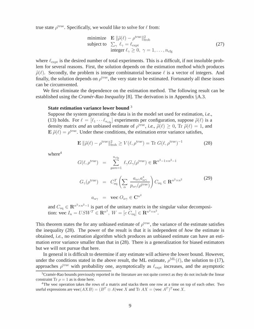
true stateρtrue. Specifically, we would like to solve forℓ from:

minimize E ‖ρ(ℓ)− ρtrue‖2frobsubject to

∑γ ℓγ = ℓexpt

integerℓγ ≥ 0, γ = 1, . . . , ncfg

(27)

whereℓexpt is the desired number of total experiments. This is a difficult, if not insoluble prob-lem for several reasons. First, the solution depends on the estimation method which producesρ(ℓ). Secondly, the problem is integer combinatorial becauseℓ is a vector of integers. Andfinally, the solution depends onρtrue, the very state to be estimated. Fortunately all these issuescan be circumvented.

We first eliminate the dependence on the estimation method. The following result can beestablished using theCramer-Rao Inequality[8]. The derivation is in Appendix§A.3.

State estimation variance lower bound3

Suppose the system generating the data is in the model set used for estimation,i.e.,(13) holds. Forℓ = [ℓ1 · · · ℓncfg

] experiments per configuration, supposeρ(ℓ) is adensity matrixandan unbiased estimate ofρtrue, i.e., ρ(ℓ) ≥ 0, Tr ρ(ℓ) = 1, andE ρ(ℓ) = ρtrue. Under these conditions, the estimation error variance satisfies,

E ‖ρ(ℓ)− ρtrue‖2frob ≥ V (ℓ, ρtrue) = Tr G(ℓ, ρtrue)−1 (28)

where4

G(ℓ, ρtrue) =ncfg∑

gam=1

ℓγGγ(ρtrue) ∈ Rn2−1×n2−1

Gγ(ρtrue) = CT

eq

(∑

α

aαγa∗αγ

pαγ(ρtrue)

)Ceq ∈ Rn2×n2

aαγ = vec Oαγ ∈ Cn2

(29)

andCeq ∈ Rn2×n2−1 is part of the unitary matrix in the singular value decomposi-tion: vec In = USW T ∈ Rn2

, W = [c Ceq] ∈ Rn2×n2

.

This theorem states the for any unbiased estimate ofρtrue, the variance of the estimate satisfiesthe inequality (28). The power of the result is that it is independent ofhow the estimate isobtained,i.e., no estimation algorithm which produces an unbiased estimate can have an esti-mation error variance smaller than that in (28). There is a generalization for biased estimatorsbut we will not pursue that here.

In general it is difficult to determine if any estimate will achieve the lower bound. However,under the conditions stated in the above result, the ML estimate,ρML(ℓ), the solution to (17),approachesρtrue with probability one, asymptotically asℓexpt increases, and the asymptotic

3Cramer-Rao bounds previously reported in the literature are not quite correct as they do not include the linearconstraintTr ρ = 1 as is done here.

4Thevec operation takes the rows of a matrix and stacks them one row ata time on top of each other. Twouseful expressions arevec(AXB) = (BT ⊗A)vec X andTr AX = (vec AT )TvecX .

9

distribution becomes Gaussian with covariance given by theCramer-Rao bound (see§A.2 forthe covariance expression and [22] for a derivation).

The one qualifier to the Cramer-Rao bound as presented is that the indicated inverse exists.This condition, however, is necessary and sufficient to insure that the state is identifiable. Moreprecisely, the state isidentifiableif and only if,

G(ℓ = 1ncfg, ρtrue) = C∗

eq

(∑

γ

∑

α

aαγa∗αγ

pαγ(ρtrue)

)Ceq is invertible (30)

Under the condition of identifiability, the experiment design problem can be expressed by thefollowing optimization problem in the vector of integersℓ:

minimize V (ℓ, ρtrue) = Tr G(ℓ, ρtrue)−1

subject to∑γ ℓγ = ℓexpt

integerℓγ ≥ 0, γ = 1, . . . , ncfg

(31)

whereℓexpt is the desired number of total experiments. The good news is that the objective,V (ℓ, ρtrue), is convex inℓ [5, §7.5]. Unfortunately, there are still two impediments: (i) restrict-ing ℓ to a vector of integers makes the problem combinatorial; (ii) the lower-bound functionV (ℓ, ρtrue) depends on the true value,ρtrue. These difficulties can be alleviated to some extent.For (i) we can use the convex relaxation described in [5,§7,5]. For (ii) we can solve the relaxedexperiment design problem with either a set of “what-if” estimates as surrogates forρtrue, oruse nominal values to start and then “bootstrap” to more precise values by iterating betweenstate estimation and experiment design. We now explain how to perform these steps.

Relaxed experiment design for state estimation

Following the procedure in [5,§7.5], introduce the variablesλγ = ℓγ/ℓexpt, each of which isthe fraction of the total number of experiments performed inconfigurationγ. Since all theℓγandℓexpt are non-negative integers, eachλγ is non-negative andrational, specifically an integermultiple of 1/ℓexpt, and in addition,

∑γ λγ = 1. Let ρsurr denote a surrogate forρtrue, e.g., an

estimate or candidate value ofρtrue. Using (28)-(29) gives,

V (ℓ = ℓexptλ, ρsurr) =

1

ℓexptV (λ, ρsurr) (32)

Using (29),V (λ, ρsurr) = Tr G(λ, ρsurr)−1

G(λ, ρsurr) =∑

γ

λγGγ(ρsurr) (33)

Hence, the objective functionV (ℓ, ρsurr) can be replaced withV (λ, ρsurr) and the experimentdesign problem (31) is equivalent to.

minimize V (λ, ρsurr) = Tr G(λ, ρsurr)−1

subject to∑γ λγ = 1

λγ ≥ 0, integer multiple of1/ℓexpt, γ = 1, . . . , ncfg

(34)

10

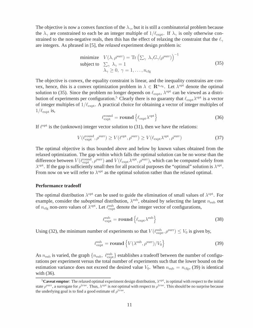
The objective is now a convex function of theλγ, but it is still a combinatorial problem becausetheλγ are constrained to each be an integer multiple of1/ℓexpt. If λγ is only otherwise con-strained to the non-negative reals, then this has the effectof relaxing the constraint that theℓγare integers. As phrased in [5], therelaxedexperiment design problem is:

minimize V (λ, ρsurr) = Tr(∑

γ λγGγ(ρsurr)

)−1

subject to∑γ λγ = 1

λγ ≥ 0, γ = 1, . . . , ncfg

(35)

The objective is convex, the equality constraint is linear,and the inequality constrains are con-vex, hence, this is a convex optimization problem inλ ∈ Rncfg . Let λopt denote the optimalsolution to (35). Since the problem no longer depends onℓexpt, λopt can be viewed as a distri-bution of experiments per configuration.5 Clearly there is no guaranty thatℓexptλopt is a vectorof integer multiples of1/ℓexpt. A practical choice for obtaining a vector of integer multiples of1/ℓexpt is,

ℓroundexpt = roundℓexptλ

opt

(36)

If ℓopt is the (unknown) integer vector solution to (31), then we have the relations:

V (ℓroundexpt , ρsurr) ≥ V (ℓopt, ρsurr) ≥ V (ℓexptλ

opt, ρsurr) (37)

The optimal objective is thus bounded above and below by known values obtained from therelaxed optimization. The gap within which falls the optimal solution can be no worse than thedifference betweenV (ℓroundexpt , ρ

surr) andV (ℓexptλopt, ρsurr), which can be computed solely fromλopt. If the gap is sufficiently small then for all practical purposes the “optimal” solution isλopt.From now on we will refer toλopt as the optimal solution rather than the relaxed optimal.

Performance tradeoff

The optimal distributionλopt can be used to guide the elimination of small values ofλopt. Forexample, consider thesuboptimaldistribution,λsub, obtained by selecting the largestnsub outof ncfg non-zero values ofλopt. Let ℓsubexpt denote the integer vector of configurations,

ℓsubexpt = roundℓexptλ

sub

(38)

Using (32), the minimum number of experiments so thatV (ℓsubexpt, ρsurr) ≤ V0 is given by,

ℓsubexpt = roundV (λsub, ρsurr)/V0

(39)

As nsub is varied, the graphnsub, ℓsubexpt establishes a tradeoff between the number of configu-

rations per experiment versus the total number of experiments such that the lower bound on theestimation variance does not exceed the desired valueV0. Whennsub = ncfg, (39) is identicalwith (36).

5Caveat emptor: The relaxed optimal experiment design distribution,λopt, is optimal with respect to the initialstateρsurr, a surrogate forρtrue. Thus,λopt is notoptimal with respect toρtrue. This should be no surprise becausethe underlying goal is to find a good estimate ofρtrue.

11

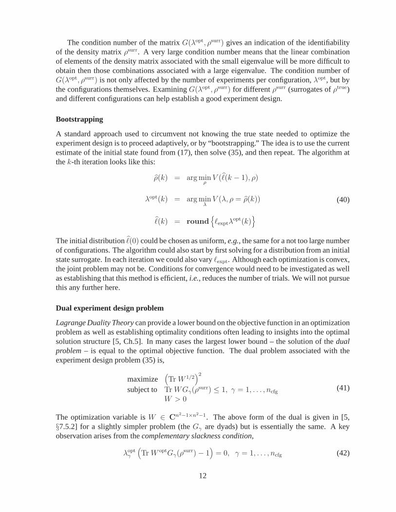
The condition number of the matrixG(λopt, ρsurr) gives an indication of the identifiabilityof the density matrixρsurr. A very large condition number means that the linear combinationof elements of the density matrix associated with the small eigenvalue will be more difficult toobtain then those combinations associated with a large eigenvalue. The condition number ofG(λopt, ρsurr) is not only affected by the number of experiments per configuration,λopt, but bythe configurations themselves. ExaminingG(λopt, ρsurr) for differentρsurr (surrogates ofρtrue)and different configurations can help establish a good experiment design.

Bootstrapping

A standard approach used to circumvent not knowing the true state needed to optimize theexperiment design is to proceed adaptively, or by “bootstrapping.” The idea is to use the currentestimate of the initial state found from (17), then solve (35), and then repeat. The algorithm atthek-th iteration looks like this:

ρ(k) = argminρV (ℓ(k − 1), ρ)

λopt(k) = argminλV (λ, ρ = ρ(k))

ℓ(k) = roundℓexptλ

opt(k)

(40)

The initial distributionℓ(0) could be chosen as uniform,e.g., the same for a not too large numberof configurations. The algorithm could also start by first solving for a distribution from an initialstate surrogate. In each iteration we could also varyℓexpt. Although each optimization is convex,the joint problem may not be. Conditions for convergence would need to be investigated as wellas establishing that this method is efficient,i.e., reduces the number of trials. We will not pursuethis any further here.

Dual experiment design problem

Lagrange Duality Theorycan provide a lower bound on the objective function in an optimizationproblem as well as establishing optimality conditions often leading to insights into the optimalsolution structure [5, Ch.5]. In many cases the largest lower bound – the solution of thedualproblem– is equal to the optimal objective function. The dual problem associated with theexperiment design problem (35) is,

maximize(TrW 1/2

)2

subject to TrWGγ(ρsurr) ≤ 1, γ = 1, . . . , ncfg

W > 0

(41)

The optimization variable isW ∈ Cn2−1×n2−1. The above form of the dual is given in [5,§7.5.2] for a slightly simpler problem (theGγ are dyads) but is essentially the same. A keyobservation arises from thecomplementary slackness condition,

λoptγ

(TrW optGγ(ρ

surr)− 1)= 0, γ = 1, . . . , ncfg (42)

12

whereλopt is the solution to theprimal problem, (35), andW opt is the solution to the dualproblem, (41). Thus, only when the equality constraint holds, Tr W optGγ(ρ

surr) = 1, is theassociatedλoptγ not necessarily equal to zero. It will therefore be usually the case that many ofthe elements of the optimal distribution will be zero.

Strong duality also holds for this problem, thus the optimalprimal and dual objective valuesare equal,

Tr

(∑

γ

λoptγ Gγ(ρsurr)

)−1

=(Tr (W opt)1/2

)2(43)

For this problem, a pair(λ, W ) is optimal with respect toρsurr if and only if:∑γ λγ = 1λγ ≥ 0, ∀γ

λoptγ (TrW optGγ(ρsurr)− 1) = 0, ∀γ

TrWGγ(ρsurr) ≤ 1, ∀γ

Tr(∑

γ λγGγ(ρsurr)

)−1=

(Tr (W opt)1/2

)2

(44)

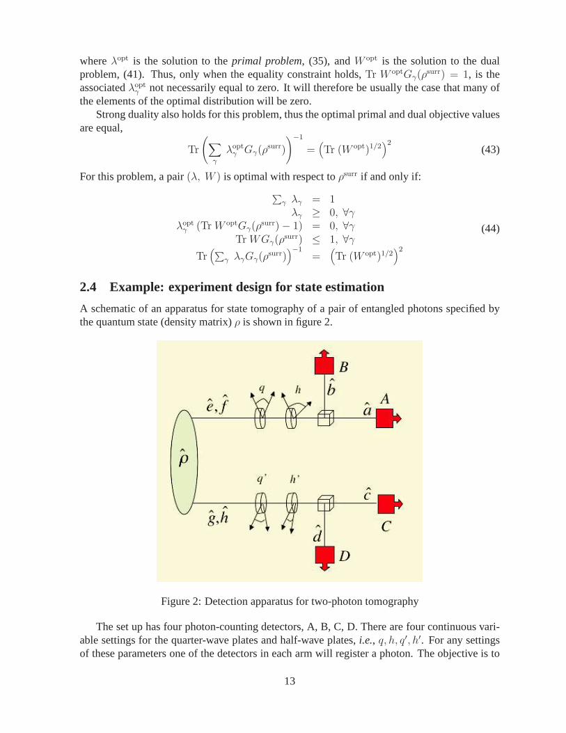
2.4 Example: experiment design for state estimation

A schematic of an apparatus for state tomography of a pair of entangled photons specified bythe quantum state (density matrix)ρ is shown in figure 2.

Figure 2: Detection apparatus for two-photon tomography

The set up has four photon-counting detectors, A, B, C, D. There are four continuous vari-able settings for the quarter-wave plates and half-wave plates,i.e., q, h, q′, h′. For any settingsof these parameters one of the detectors in each arm will register a photon. The objective is to

13

determine the optimal settings of these parameters and the number of experiments per settingfor estimation of the stateρ of the pair using as data the photon counts from the four detectors.

Because the photon sources are not completely efficient, theinput quantum state actu-ally consists of either two or zero photons. The detectors register a 0 or 1 depending onwhether a photon is incident on them or not. The basis states for the upper arm are therefore:|0〉e|0〉f , |0〉e|1〉f , |1〉e|0〉f . There is a similar set for the lower arm (modesg, h).

The firing patterns for an arbitrary setting of the wave plates, assuming perfect detectionefficiency and no dark counts are given in the table:

A B C D0 1 0 10 1 1 01 0 0 11 0 1 00 0 0 0

The probabilities for these patterns are given by

pijkℓ = Tr (M ijAB ⊗Mkℓ

CD)ρ (45)

wherei, j, k, ℓ ∈ 0, 1, andM ijAB is the projector for detector A to register counti and

simultaneously detector B to register countj. Similarly,MkℓCD is the projector for detector C to

register countj and simultaneously detector D to register countℓ. The projectors for A and Bin the above basis are:

M00AB =

1 0 00 0 00 0 0

M10AB =

[0

ψ1(h, q)

][0 ψ1(h, q)

∗] , ψ1(h, q) =1√2

[sin 2h+ i sin 2(h− q)cos 2h− i cos 2(h− q)

]

M01AB =

[0

ψ2(h, q)

][0 ψ2(h, q)

∗] , ψ2(h, q) =1√2

[cos 2h+ i cos 2(h− q)− sin 2h+ i sin 2(h− q)

]

(46)

A similar set of projectors can be written for C and D with the variablesh, q replaced by theirprimed counterpartsh′, q′.

The protocol is to measure the probabilities for enough settings of the variables that theelements of the two-photon density operator can be estimated. The two-photon density operatoris the direct product of the one-photon density operator, for which the set of 3 states given aboveforms a basis. The basis states of the two-photon(9 × 9) density operator,ρ, are: |ijkℓ〉 =|i〉e|j〉f |k〉g|ℓ〉h with i, j, k, ℓ ∈ 0, 1 Hence,

zero photon |0000〉one photon |0100〉, |1000〉, |0001〉, |0010〉two photon |0101〉, |0110〉, |1001〉, |1010〉

14

simulation results: one-arm

Consider only one arm of the apparatus in figure 2, say the upper arm with detectors (A,B).Suppose the wave plate settings are,

hγ, qγ | γ = 1, . . . , ncfg (47)

Assume also that the incoming statealwaysis one photon, never none. Hence,ρ ∈ C2×2 andthe projectors are:

M10γ = ψ1(hγ , qγ)ψ1(hγ, qγ)

∗

M01γ = ψ2(hγ , qγ)ψ2(hγ, qγ)

∗(48)

with ψ1, ψ2 from (46). Assuming each detector has efficiencyη, 0 ≤ η ≤ 1 and a non-zerodark count probability,δ, 0 ≤ δ ≤ 1, then there are four possible outcomes at detectors A,Bgiven in the following table:

α A B10 1 001 0 100 0 011 1 1

Following [15, 39] the probability of a dark count is denotedby the conditional probability,

ν1|0 = δ (49)

where1|0 means the detector has fired “1” given that no photon is present at the detector “0.”As shown in [15], it therefore follows that the probability that the detector does not fire “0”although a photon is present at the detector “1” is given by,

ν0|1 = (1− η)(1− δ) (50)

Here1 − η is the probability of no detection and1− δ is the probability of no dark count. Theremaining conditional probabilities are, by definition, constrained to obey:

ν1|0 + ν0|0 = 1ν1|1 + ν0|1 = 1

(51)

The probabilities for the firing patterns in the above table are thus given by (7) with the followingobservablesMαγ :

M10,γ = ν1|1ν0|0M10γ + ν1|0ν0|1M

01γ

M01,γ = ν0|1ν1|0M10γ + ν0|0ν1|1M

01γ

M00,γ = ν0|1ν0|0M10γ + ν0|0ν0|1M

01γ

M11,γ = ν1|1ν1|0M10γ + ν1|0ν1|1M

01γ

(52)

15

Numerical computer simulations were performed for two input state cases:

pure state: ρpure =1

2

[1 11 1

]= ψ0ψ∗, ψ0 =

1√2

[11

]

mixed state: ρmixd =

[0.6 −0.2i0.2i 0.4

] (53)

For each input state case we computedλopt with and without “noise:”

no noise

detector efficiency η = 1dark count probability δ = 0

yes noise

detector efficiency η = 0.75dark count probability δ = 0.05

(54)

For all cases and noise conditions we used the wave plate settings:

hi = (i− 1)(5), i = 1, . . . , 10qi = (i− 1)(5), i = 1, . . . , 10

(55)

Both angles are set from0 to 45 in 5 increments. This yields a total ofncfg = 102 = 100configurations corresponding to all the wave plate combinations.

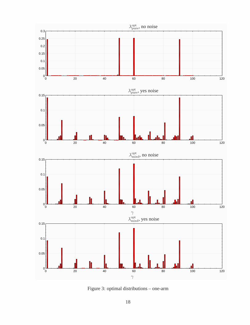
Figure 3 shows the optimal distributionsλopt versus configurationsγ = 1, . . . , 100 for allfour test cases: two input states with and without noise. Observe that the optimal distributionsarenotuniform but are concentrated near the same particular wave plate settings. These settingsare very close to those established in [17].

To check the gap between the relaxed optimumλopt and the unknown integer optimum weappeal to (36)-(37). The following table shows that these distributions are good approximationto the unknown optimal integer solution for even not so largeℓexpt for the two state cases withno noise. Similar results were obtained for the noisy case.

ℓexptV (ℓexptλ

optpure, ρpure)

V (ℓroundexpt (ρpure), ρpure)

V (ℓexptλoptmixd, ρmixd)

V (ℓroundexpt (ρmixd), ρmixd)

100 .9797 .77611000 .9950 .973510, 000 .9989 .9954

The following table compares the distributions for optimal, suboptimal with 8 angles, uniformat the 8 suboptimal angles, and uniform at all 100 angles by computing the minimum number

16

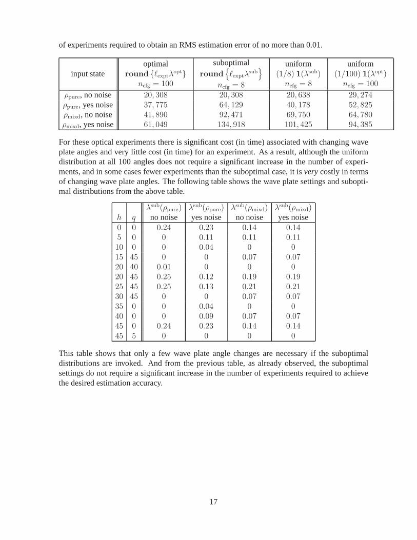
of experiments required to obtain an RMS estimation error ofno more than 0.01.

input stateoptimal

round ℓexptλoptncfg = 100

suboptimalround

ℓexptλ

sub

ncfg = 8

uniform(1/8) 1(λsub)ncfg = 8

uniform(1/100) 1(λopt)ncfg = 100

ρpure, no noise 20, 308 20, 308 20, 638 29, 274ρpure, yes noise 37, 775 64, 129 40, 178 52, 825ρmixd, no noise 41, 890 92, 471 69, 750 64, 780ρmixd, yes noise 61, 049 134, 918 101, 425 94, 385

For these optical experiments there is significant cost (in time) associated with changing waveplate angles and very little cost (in time) for an experiment. As a result, although the uniformdistribution at all 100 angles does not require a significantincrease in the number of experi-ments, and in some cases fewer experiments than the suboptimal case, it isverycostly in termsof changing wave plate angles. The following table shows thewave plate settings and subopti-mal distributions from the above table.

λsub(ρpure) λsub(ρpure) λsub(ρmixd) λsub(ρmixd)h q no noise yes noise no noise yes noise0 0 0.24 0.23 0.14 0.145 0 0 0.11 0.11 0.1110 0 0 0.04 0 015 45 0 0 0.07 0.0720 40 0.01 0 0 020 45 0.25 0.12 0.19 0.1925 45 0.25 0.13 0.21 0.2130 45 0 0 0.07 0.0735 0 0 0.04 0 040 0 0 0.09 0.07 0.0745 0 0.24 0.23 0.14 0.1445 5 0 0 0 0

This table shows that only a few wave plate angle changes are necessary if the suboptimaldistributions are invoked. And from the previous table, as already observed, the suboptimalsettings do not require a significant increase in the number of experiments required to achievethe desired estimation accuracy.

17

20 40 60 80 1000 120

0.05

0.1

0.15

0.2

0.25

0

0.3

20 40 60 80 1000 120

0.05

0.1

0

0.15

20 40 60 80 1000 120

0.05

0.1

0

0.15

20 40 60 80 1000 120

0.05

0.1

0

0.15

PSfrag replacements

γ

γ

λoptpure, no noise

λoptpure, yes noise

λoptmixd, no noise

λoptmixd, yes noise

Figure 3: optimal distributions – one-arm

18

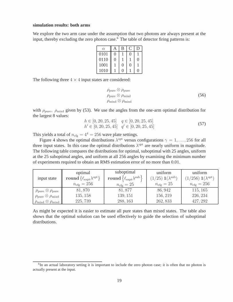
simulation results: both arms

We explore the two arm case under the assumption that two photons are always present at theinput, thereby excluding the zero photon case.6 The table of detector firing patterns is:

α A B C D0101 0 1 0 10110 0 1 1 01001 1 0 0 11010 1 0 1 0

The following three4× 4 input states are considered:

ρpure ⊗ ρpureρpure ⊗ ρmixd

ρmixd ⊗ ρmixd

(56)

with ρpure, ρmixd given by (53). We use the angles from the one-arm optimal distribution forthe largest 8 values:

h ∈ [0, 20, 25, 45] q ∈ [0, 20, 25, 45]h′ ∈ [0, 20, 25, 45] q′ ∈ [0, 20, 25, 45]

(57)

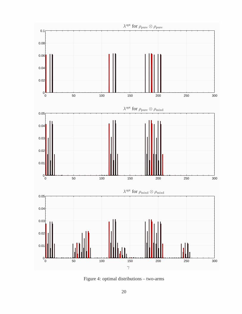
This yields a total ofncfg = 44 = 256 wave plate settings.Figure 4 shows the optimal distributionsλopt versus configurationsγ = 1, . . . , 256 for all

three input states. In this case the optimal distributionsλopt are nearly uniform in magnitude.The following table compares the distributions for optimal, suboptimal with 25 angles, uniformat the 25 suboptimal angles, and uniform at all 256 angles by examining the minimum numberof experiments required to obtain an RMS estimation error ofno more than 0.01.

input stateoptimal

round ℓexptλoptncfg = 256

suboptimalround

ℓexptλ

sub

ncfg = 25

uniform(1/25) 1(λsub)ncfg = 25

uniform(1/256) 1(λopt)ncfg = 256

ρpure ⊗ ρpure 81, 870 81, 877 86, 942 115, 165ρpure ⊗ ρmixd 135, 158 139, 151 156, 219 226, 234ρmixd ⊗ ρmixd 225, 739 288, 163 262, 833 427, 292

As might be expected it is easier to estimate all pure states than mixed states. The table alsoshows that the optimal solution can be used effectively to guide the selection of suboptimaldistributions.

6In an actual laboratory setting it is important to include the zero photon case; it is often that no photon isactually present at the input.

19

50 100 150 200 2500 300

0.02

0.04

0.06

0.08

0

0.1

50 100 150 200 2500 300

0.01

0.02

0.03

0.04

0

0.05

50 100 150 200 2500 300

0.01

0.02

0.03

0.04

0

0.05

PSfrag replacements

γλoptpure, no noiseλoptpure, yes noiseλoptmixd, no noiseλoptmixd, yes noise

γ

λopt for ρpure ⊗ ρpure

λopt for ρpure ⊗ ρmixd

λopt for ρmixd ⊗ ρmixd

Figure 4: optimal distributions – two-arms

20

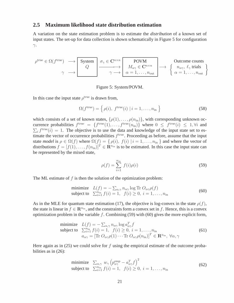
2.5 Maximum likelihood state distribution estimation

A variation on the state estimation problem is to estimate the distribution of a known set ofinput states. The set-up for data collection is shown schematically in Figure 5 for configurationγ.

ρtrue ∈ Ω(f true) −→

γ −→

SystemQ

σγ ∈ Cn×n

———-−→γ −→

POVMMαγ ∈ Cn×n

α = 1, . . . , nout

−→Outcome countsnαγ , ℓγ trialsα = 1, . . . , nout

Figure 5: System/POVM.

In this case the input stateρtrue is drawn from,

Ω(f true) =ρ(i), f true(i) | i = 1, . . . , nin

(58)

which consists of a set of known states,ρ(1), . . . , ρ(nin), with corresponding unknown oc-currence probabilitiesf true = f true(1), . . . , f true(nin) where 0 ≤ f true(i) ≤ 1, ∀i and∑i f

true(i) = 1. The objective is to use the data and knowledge of the input state set to es-timate the vector of occurrence probabilitiesf true. Proceeding as before, assume that the inputstatemodelis ρ ∈ Ω(f) whereΩ(f) = ρ(i), f(i) | i = 1, . . . , nin and where the vector ofdistributionsf = [f(1), . . . , f(nin)]

T ∈ Rnin is to be estimated. In this case the input state canbe represented by the mixed state,

ρ(f) =nin∑

i=1

f(i)ρ(i) (59)

The ML estimate off is then the solution of the optimization problem:

minimize L(f) = −∑α,γ nαγ log Tr Oαγρ(f)subject to

∑nin

i=1 f(i) = 1, f(i) ≥ 0, i = 1, . . . , nin(60)

As in the MLE for quantum state estimation (17), the objective is log-convex in the stateρ(f),the state is linear inf ∈ Rnin, and the constraints form a convex set inf . Hence, this is a convexoptimization problem in the variablef . Combining (59) with (60) gives the more explicit form,

minimize L(f) = −∑α,γ nαγ log aTαγf

subject to∑nin

i=1 f(i) = 1, f(i) ≥ 0, i = 1, . . . , nin

aαγ = [Tr Oαγρ(1) · · ·Tr Oαγρ(nin)]T ∈ Rnin, ∀α, γ

(61)

Here again as in (25) we could solve forf using the empirical estimate of the outcome proba-bilities as in (26):

minimize∑α,γ wγ

(pempαγ − aTαγf

)2

subject to∑nin

i=1 f(i) = 1, f(i) ≥ 0, i = 1, . . . , nin

(62)

21

2.6 Experiment design for state distribution estimation

Let f surr ∈ Rnin be a surrogate for the true state distribution,f true. Following the derivation of(28) in Appendix§A.3, the associated (relaxed) optimal experiment design problem is,

minimize V (λ, f surr) = Tr(∑

γ λγGγ(fsurr)

)−1

subject to∑γ λγ = 1

λγ ≥ 0, γ = 1, . . . , ncfg

(63)

where

Gγ(fsurr) = CT

eq

(∑

α

aαγaTαγ

pαγ(f surr)

)Ceq ∈ Rnin−1×nin−1 (64)

with aαγ ∈ Rnin from (60) and whereCeq ∈ Rnin×nin−1 is part of the unitary matrixW in thesingular value decomposition:1Tnin

= USW T , W = [c Ceq] ∈ Rnin×nin.

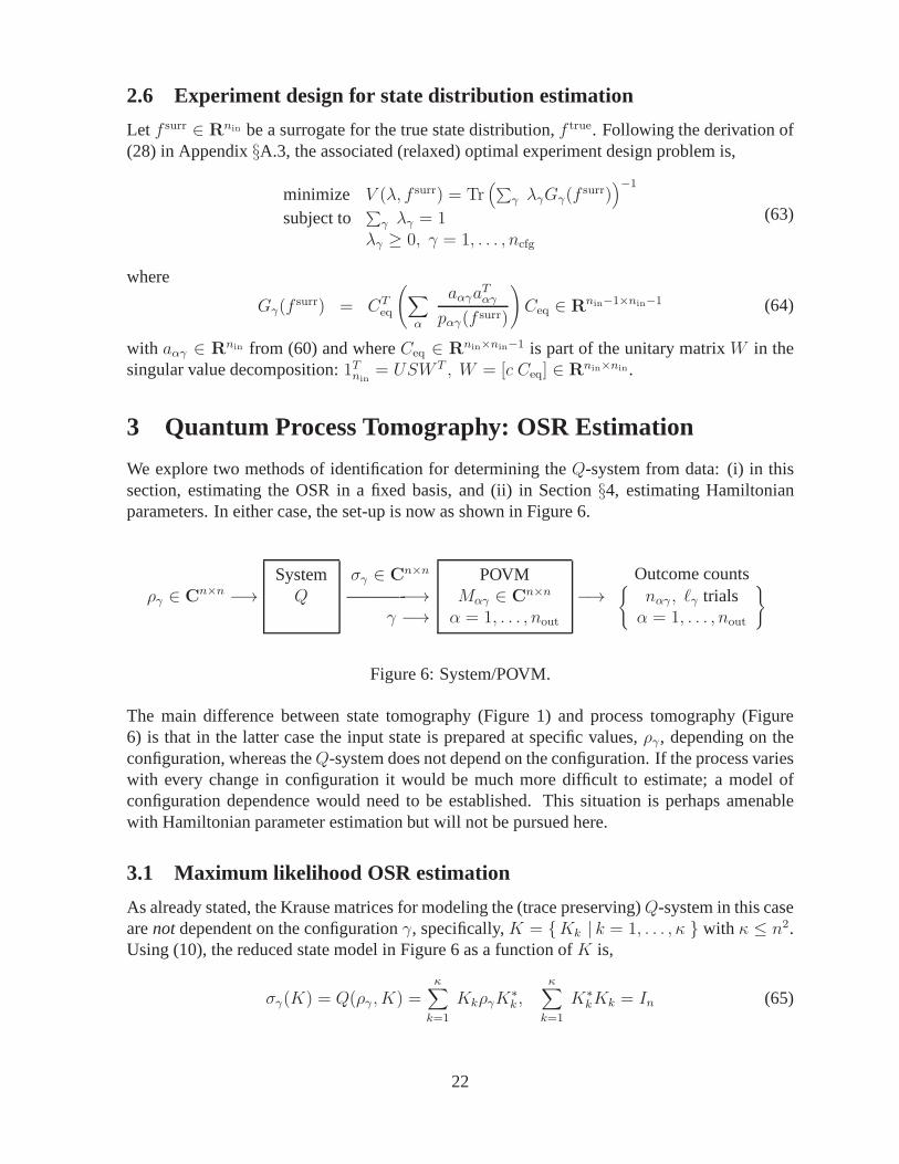
3 Quantum Process Tomography: OSR Estimation

We explore two methods of identification for determining theQ-system from data: (i) in thissection, estimating the OSR in a fixed basis, and (ii) in Section §4, estimating Hamiltonianparameters. In either case, the set-up is now as shown in Figure 6.

ργ ∈ Cn×n −→SystemQ

σγ ∈ Cn×n

———-−→γ −→

POVMMαγ ∈ Cn×n

α = 1, . . . , nout

−→Outcome countsnαγ , ℓγ trialsα = 1, . . . , nout

Figure 6: System/POVM.

The main difference between state tomography (Figure 1) andprocess tomography (Figure6) is that in the latter case the input state is prepared at specific values,ργ , depending on theconfiguration, whereas theQ-system does not depend on the configuration. If the process varieswith every change in configuration it would be much more difficult to estimate; a model ofconfiguration dependence would need to be established. Thissituation is perhaps amenablewith Hamiltonian parameter estimation but will not be pursued here.

3.1 Maximum likelihood OSR estimation

As already stated, the Krause matrices for modeling the (trace preserving)Q-system in this casearenotdependent on the configurationγ, specifically,K = Kk | k = 1, . . . , κ with κ ≤ n2.Using (10), the reduced state model in Figure 6 as a function of K is,

σγ(K) = Q(ργ , K) =κ∑

k=1

KkργK∗k ,

κ∑

k=1

K∗kKk = In (65)

22

Combining the above with the measurement model (9) gives theprobability outcomes model,

pαγ(K) = Tr Oαγ(K)ργ , Oαγ(K) =κ∑

k=1

K∗kMαγKk (66)

The log-likelihood function (16) is,

L(D,K) = −∑

α,γ

nαγ log Tr Oαγ(K)ργ (67)

An ML estimate ofK is then a solution to,

minimize L(D,K) = −∑α,γ nαγ log Tr∑κk=1 K

∗kMαγKkργ

subject to∑κk=1 K

∗kKk = In

(68)

This is not a convex optimization for two reasons: the equality constraint is not linear inKand the objective function is not convex. The problem can be transformed – more accurately,embedded – into a convex optimization problem by expanding the Kraus matrices in a fixedbasis. The procedure, described in [27,§8.4.2], is as follows: since any matrix inCn×n can berepresented byn2 complex numbers, let

Bi ∈ Cn×n

∣∣∣ i = 1, . . . , n2

(69)

be a basis for matrices inCn×n. The Kraus matrices can thus be expressed as,

Kk =n2∑

i=1

akiBi, k = 1, . . . , κ (70)

where then2 coefficientsaki are complex scalars. Introduce the matrixX ∈ Cn2×n2

, oftenreferred to as thesuperoperator, with elements,

Xij =κ∑

k=1

a∗kiakj, i, j = 1, . . . , n2 (71)

As shown in [27], from the requirement to preserve probability, X is restricted to the convexset,

X ≥ 0,n2∑

i,j=1

Xij B∗iBj = In (72)

The system output state (65) and outcome probabilities (66)now become,

σγ(X) = Q(ργ, X) =n2∑

i,j=1

Xij BiργB∗j

pαγ(X) = Tr Oαγ Q(ργ , X) = Tr XRαγ

(73)

where the matrixRαγ ∈ Cn2×n2

has elements,

[Rαγ ]ij = Tr BjργB∗iOαγ, i, j = 1, . . . , n2 (74)

23

Quantum process tomography is then estimatingX ∈ Cn2×n2

from the data setD (4). An MLestimate is obtained by solving forX from:

minimize L(D,X) = −∑α,γ nαγ log Tr XRαγ

subject to X ≥ 0,∑ij Xij B

∗iBj = In

(75)

This problem has essentially the same form as (17), and henceis also a convex optimizationproblem with the optimization variables being the elementsof the matrixX. SinceX = X∗ ∈Cn2×n2

, it can be parametrized byn4 real variables. Accounting for then2 real linear equalityconstraints, the number of free (real) variables inX is thusn4−n2. This can be quite large evenfor a relatively small number of qubits,e.g., for q = [1, 2, 3, 4] qubits,n = 2q = [2, 4, 8, 16]andn4−n2 = [12, 240, 4032, 65280]. This exponential (in qubit) growth is the main drawbackto using this approach.

TheX (superoperator) matrix can be transformed back to Kraus operators via the singularvalue decomposition [27,§8.4.2]. Specifically, letX = V SV ∗ with unitaryV ∈ Cn2×n2

andS = diag(s1 · · · sn2) with the singular values ordered so thats1 ≥ s2 ≥ · · · ≥ sn2 ≥ 0. Thenthe coefficients in the basis representation of the Kraus matrices (70) are,

aki =√sk V

∗ik, k, i = 1, . . . , n2 (76)

Theoretically there can be fewer thenn2 Kraus operators. For example, if theQ system isunitary, then,

Q(ρ) = UρU∗ (77)

In effect, there is one Kraus operator,U , which is unitary and of the same dimension as theinput stateρ. The correspondingX matrix is a dyad, hencerank X = 1. A rank constraintis not convex. However, theX matrix is symmetric and positive semidefinite, so the heuristicfrom [10] applies where the rank constraint is replaced by the trace constraint,

Tr X ≤ η (78)

From the singular value decomposition ofX, Tr X =∑k sk, and hence, adding the constraint

(78) to (75) will force some (or many) of thesk to be small which can be eliminated (post-optimization) thereby reducing the rank. The auxiliary parameterη can be used to find a tradeoffbetween simpler realizations and performance. The estimation problem is then:

minimize L(D,X) = −∑α,γ nαγ log Tr XRαγ

subject to X ≥ 0,∑ij Xij B

∗iBj = In

Tr X ≤ η(79)

3.2 Experiment design for OSR estimation

LetXsurr ∈ Cn2×n2

be a surrogate for the true OSR,Xtrue. As derived in Appendix§A.4, theassociated (relaxed) optimal experiment design problem is,

minimize V (λ,Xsurr) = Tr(∑

γ λγGγ(Xsurr)

)−1

subject to∑γ λγ = 1

λγ ≥ 0, γ = 1, . . . , ncfg

(80)

24

where

Gγ(Xsurr) = C∗

eq

(∑

α

aαγa∗αγ

pαγ(Xsurr)

)Ceq

aαγ = vec Rαγ ∈ Cn4

(81)

andCeq ∈ Cn4×n4−n2

is part of the unitary matrixW = [C Ceq] ∈ Cn4×n4

in the singular valuedecomposition of then2 × n4 matrix,

[a1 · · · an4 ] = U[√nIn2 0n2×n4−n2

]W ∗ (82)

with with ak = vec(B∗iBj) ∈ Cn2

for k = i + (j − 1)n2, i, j = 1, . . . , n2. The columns ofCeq, i.e., the lastn4 − n2 columns ofW , are a basis for the nullspace of[a1 · · · an4 ].

3.3 Example: experiment design for OSR estimation

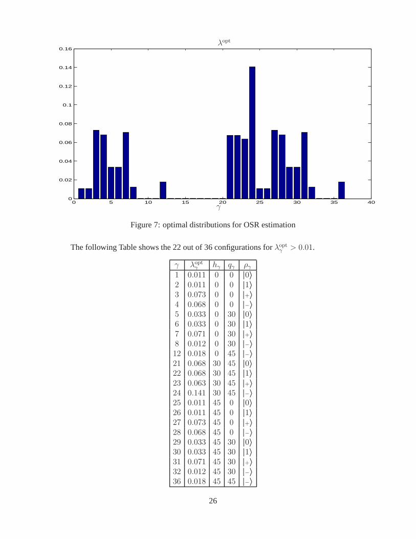
Consider the POVM set from the one-arm photon detector (§2.4) using all combinations of thefollowing set wave-plate angles,

h = [0 30 45], q = [0 30 45]

Assume detector efficiencyη = 0.75 and dark count probabilityδ = 0.05. The set of inputs(state configurations) is

|0〉, |1〉, |+〉 = (|0〉+ |1〉)/√2, |−〉 = (|0〉+ i|1〉)/

√2

The 9 combinations of angles together with the 4 combinations of input states gives a total of36 configurations,γ = 1, . . . , ncfg = 36.

Figure 7 shows the optimal distribution of experiments for the 36 configurations using thetrue OSR corresponding to the Pauli basis set

I2/

√2, σx/

√2, σy/

√2, σz/

√2. Since the

system is simply the identity,Q(ρ) = ρ, with this basis choice,Xtrue = diag(2 0 0 0). (Noknowledge of the system being identity is used, hence, all elements ofXtrue are estimated, notjust the single element in the “11” location.)

The following table displays the minimum number of experiments required to meet estima-tion accuracies of 0.05 and 0.01 for both uniform and optimaldistributions.

accuracy λopt λunif

0.01 856, 676 1, 304, 5610.05 34, 268 52, 183

Approximately 35% fewer experiments are needed using the optimal distribution. Although notdramatic, as in the photon estimation example§2.4, there is a large penalty, in terms of time,for changing wave-plate angles.

25

0 5 10 15 20 25 30 35 400

0.02

0.04

0.06

0.08

0.1

0.12

0.14

0.16

PSfrag replacements

γλoptpure, no noiseλoptpure, yes noiseλoptmixd, no noiseλoptmixd, yes noise

γλopt for ρpure ⊗ ρpureλopt for ρpure ⊗ ρmixd

λopt for ρmixd ⊗ ρmixd

γ

λopt

Figure 7: optimal distributions for OSR estimation

The following Table shows the 22 out of 36 configurations forλoptγ > 0.01.

γ λoptγ hγ qγ ργ1 0.011 0 0 |0〉2 0.011 0 0 |1〉3 0.073 0 0 |+〉4 0.068 0 0 |−〉5 0.033 0 30 |0〉6 0.033 0 30 |1〉7 0.071 0 30 |+〉8 0.012 0 30 |−〉12 0.018 0 45 |−〉21 0.068 30 45 |0〉22 0.068 30 45 |1〉23 0.063 30 45 |+〉24 0.141 30 45 |−〉25 0.011 45 0 |0〉26 0.011 45 0 |1〉27 0.073 45 0 |+〉28 0.068 45 0 |−〉29 0.033 45 30 |0〉30 0.033 45 30 |1〉31 0.071 45 30 |+〉32 0.012 45 30 |−〉36 0.018 45 45 |−〉

26

3.4 Maximum likelihood OSR distribution estimation

Suppose the Kraus matrices are known up to a scale factor which is related to its probability ofoccurrence, that is,

Kk =√qk Kk

∑κk=1 qkK

∗kKk = In∑κ

k=1 qk = 1 qk ≥ 0 k = 1, . . . , κ(83)

One interpretation of this system model is that one of the matrices, sayK1, is the nominal (un-perturbed) system, and the others,Kk, k = 2, . . . , κ, are perturbations, each of them occurringwith probabilityqk. Examples of perturbations include the typical errors which can be handledby quantum error correction codes,e.g., depolarization, phase damping, phase and bit flip; see,e.g., [27, Ch.8].

The goal is to use the data to estimate the unknown vector of probabilities,q = [q1 · · · qκ]T ∈Rκ. Using the system model (83), the model probability outcomes are,

pαγ = TrMαγ∑κk=1 qk KkργK

∗k = aTαγq

aαγ =[TrMαγK1ργK

∗1 · · ·TrMαγKκργK

∗κ

]T ∈ Rκ(84)

The ML estimate ofq ∈ Rκ is the solution of the optimization problem,

minimize L(q) = −∑α,γ nαγ log aTαγq

subject to∑κk=1 qk = 1, qk ≥ 0, k = 1, . . . , κ

(85)

This is a convex optimization problem and is essentially in the same form as problem (60) whichseeks the ML estimate of the input state distribution.

3.5 Experiment design for OSR distribution estimation

The formulation here is directly analogous to that of experiment design for state distributionestimation§2.6. Letqsurr ∈ Rnin be a surrogate for the true OSR distribution,qtrue. Followingthe lines of the derivation in Appendix§A.4, the associated (relaxed) optimal experiment designproblem is,

minimize V (λ, qsurr) = Tr(∑

γ λγGγ(qsurr)

)−1

subject to∑γ λγ = 1

λγ ≥ 0, γ = 1, . . . , ncfg

(86)

where

Gγ(qsurr) = CT

eq

(∑

α

aαγaTαγ

pαγ(qsurr)

)Ceq ∈ Rnin−1×nin−1 (87)

with aαγ ∈ Rnin from (85) and whereCeq ∈ Rnin×nin−1 is part of the unitary matrixW in thesingular value decomposition:1Tnin

= USW T , W = [c Ceq] ∈ Rnin×nin.

27

3.6 Example: experiment design for OSR distribution estimation

Consider a quantum process, or channel, where a single qubitstate,ρ ∈ C2×2, is corruptedby a bit-flip error with occurrence probabilityqB and adepolarizing errorwith occurrenceprobabilityqD. The process is described by the quantum operation,7

Q(ρ, q) = qI ρ+ qB XρX + qD I/2

qI + qB + qD = 1(88)

whereqI = 1− (qB + qD) is the probability of no error occurring. The probability ofobservingoutcomeα with the system in configurationγ is,8

pαγ(q) = TrMαγQ(ργ , q)

=[TrMαγργ TrMαγXργX TrMαγ/2

]qIqBqD

= aTαγ q

(89)

An interesting aspect of this problem is that not all input statesργ lead to identifiability of theoccurrence probabilities. And this is independent of the choice of POVMMαγ . To see thisconsider the single pure input state,

ργ = ψψ∗, ψ =

[ab

], |a|2 + |b|2 = 1 (90)

The output of the channel (88) is then,

Q(ψψ∗, q) =

[qI |a|2 + qB|b|2 + qD/2 qIab

∗ + qBa∗b

qIa∗b+ qBab

∗ qI |b|2 + qB|a|2 + qD/2

](91)

Suppose we knew the elements ofQ(ψψ∗, q) perfectly; call themQ11, Q12, Q22. Then in prin-cipal we could solve for the three occurrence probabilitiesfrom the linear system of equations,

|a|2 |b|2 1/2|b|2 |a|2 1/2ab∗ a∗b 0

︸ ︷︷ ︸R

qIqBqD

=

Q11

Q22

Q12

(92)

If det R = 0 then no unique solution exists; the occurrence probabilities are notidentifiable.Specifically,det R = 0 for all a, b ∈ C such that,

(Re ab∗)(|b|2 − |a|2) = 0, |a|2 + |b|2 = 1 (93)

7X is one of the three2× 2 Pauli spin matrices:X =

[0 11 0

], Y =

[0 −ii 0

], Z =

[1 00 −1

]

8As shown in [27, §8.3], an equivalent set of OSR elements which describe (88) are,√qI I,

√qB X,

√qD I/2,

√qD X/2,

√qD Y/2,

√qD Z/2. Forming the probability outcomes in terms

of this expansion results in an overparamtrization.

28

Equivalently,det R = 0 for the following sets ofa, b ∈ C:

(a = 0, |b| = 1), (|a| = 1, b = 0), (|a| = |b| = 1/√2) (94)

Let the input state be a single pure state of the form

ψ(θ) =

[cos θsin θ

], (95)

Suppose the angleθ is restricted to the range0 ≤ θ ≤ 90. Using (94), the occurrence proba-bilities are not identifiable for the anglesθ. and respectively, the statesψ(θ), in the sets,

θ ∈ 0, 45, 90 , ψ(θ) ∈[

10

],

[1/√2

1/√2

],

[01

](96)

Unfortunately, this excludes inputs identical to the computational basis states|0〉 or |1〉, respec-tively, ψ(θ) with θ = 0 or θ = 90.

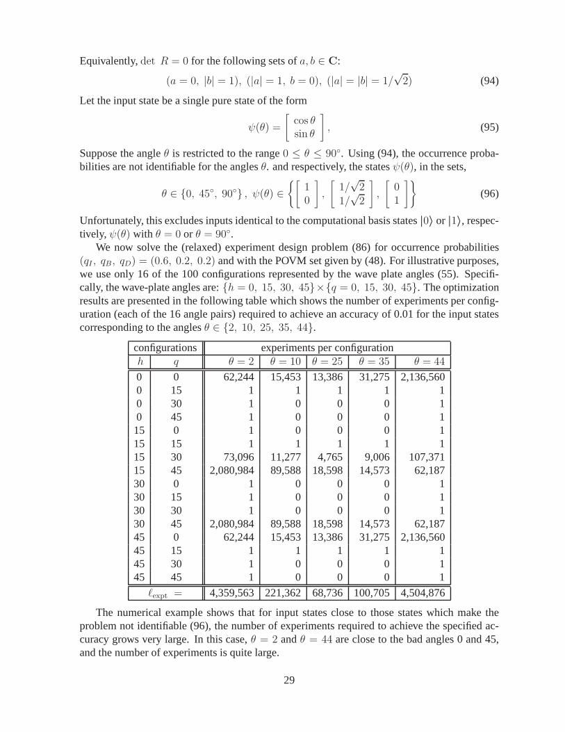
We now solve the (relaxed) experiment design problem (86) for occurrence probabilities(qI , qB, qD) = (0.6, 0.2, 0.2) and with the POVM set given by (48). For illustrative purposes,we use only 16 of the 100 configurations represented by the wave plate angles (55). Specifi-cally, the wave-plate angles are:h = 0, 15, 30, 45×q = 0, 15, 30, 45. The optimizationresults are presented in the following table which shows thenumber of experiments per config-uration (each of the 16 angle pairs) required to achieve an accuracy of 0.01 for the input statescorresponding to the anglesθ ∈ 2, 10, 25, 35, 44.

configurations experiments per configurationh q θ = 2 θ = 10 θ = 25 θ = 35 θ = 44

0 0 62,244 15,453 13,386 31,275 2,136,5600 15 1 1 1 1 10 30 1 0 0 0 10 45 1 0 0 0 115 0 1 0 0 0 115 15 1 1 1 1 115 30 73,096 11,277 4,765 9,006 107,37115 45 2,080,984 89,588 18,598 14,573 62,18730 0 1 0 0 0 130 15 1 0 0 0 130 30 1 0 0 0 130 45 2,080,984 89,588 18,598 14,573 62,18745 0 62,244 15,453 13,386 31,275 2,136,56045 15 1 1 1 1 145 30 1 0 0 0 145 45 1 0 0 0 1

ℓexpt = 4,359,563 221,362 68,736 100,705 4,504,876

The numerical example shows that for input states close to those states which make theproblem not identifiable (96), the number of experiments required to achieve the specified ac-curacy grows very large. In this case,θ = 2 andθ = 44 are close to the bad angles 0 and 45,and the number of experiments is quite large.

29

4 Hamiltonian Parameter Estimation

The process of modeling a quantum system in this case begins with the construction of a Hamil-tonianoperatoron an infinite dimensional Hilbert space.Eventually, a finite dimensional ap-proximation is invoked in order to calculate anything. (In some cases a finite dimensional modelis immediately appropriate,e.g., spin systems, [11, Ch.12-9].) The finite dimensional modelisthe starting point here.

4.1 Maximum likelihood Hamiltonian parameter estimation

The quantum system is modeled by a finite dimensional Hamiltonian matrixH(t, θ) ∈ Cn×n,having a known dependence on timet, 0 ≤ t ≤ tf , and on an unknown parameter vectorθ ∈ Rnθ . The model density matrix will depend onθ and the initial (prepared and known)state drawn from the set of states

ρinitβ ∈ Cn×n |β = 1, . . . , nin

. Thus, the density matrix

associated with initial stateρinitβ is ρβ(t, θ) ∈ Cn×n which evolves according to,

ih−ρβ = [H(t, θ), ρβ], ρβ(0, θ) = ρinitβ (97)

Equivalently,ρβ(t, θ) = U(t, θ)ρinitβ U(t, θ)∗ (98)

whereU(t, θ) ∈ Cn×n is the unitary propagator associated withH(t, θ) which satisfies,

ih−U = H(t, θ)U, U(0, θ) = In (99)

At each ofnsa sample times in a time interval of durationtf , measurements are recorded fromidentical repeated experiments. Specifically, let tτ | τ = 1, . . . , nsa denote the sample timesrelative to the start of each experiment. Letnαβτ be the number of times the outcomeα isrecorded attτ with initial stateρinitβ from ℓβτ experiments. The data set thus consists of all theoutcome counts,

D = nαβτ |α = 1, . . . , nout, β = 1, . . . , nin, τ = 1, . . . , nsa (100)

Theconfigurationspreviously enumerated and labeled byγ = 1, . . . , ncfg are in this case all thecombinations of input statesρinitβ and sample timesτ , thusncfg = ninnsa. For the POVMMα,the model outcome probability per configuration pair(ρinitβ , tτ ) is,

pαβτ (θ) = TrMαρβ(tτ , θ) = Tr Oατ (θ)ρinitβ

Oατ (θ) = U(tτ , θ)∗MαU(tτ , θ)

(101)

The Maximum Likelihood estimate,θML ∈ Rnθ , is obtained as the solution to the optimizationproblem:

minimize L(D, θ) = −∑α,β,τ nαβτ log Tr Oατ (θ)ρinitβ

subject to θ ∈ Θ(102)

whereΘ is a set of constraints onθ. For example, it may be known thatθ is restricted toa region near a nominal value,e.g., Θ = θ | ‖θ − θnom‖ ≤ δ . Although this latter set isconvex, unfortunately, the likelihood function,L(D, θ), is not guaranteed to be convex inθ. Itis possible, however, that it is convex in the restricted regionΘ, for example, ifδ is sufficientlysmall.

30

4.2 Experiment design for Hamiltonian parameter estimation

Despite the fact that Hamiltonian parameter estimation is not convex, the (relaxed) experimentdesign problem is convex. A direct application of the Cramer-Rao bound to the likelihoodfunction in (102) results in the following.

Hamiltonian parameter estimation variance lower boundSuppose the systemgenerating the data is in the model set used for estimation,i.e., (13) holds. Forℓ = [ℓ1 · · · ℓncfg

] experiments per configuration(ρinitβ , tτ ), supposeθ(ℓ) ∈ Rnθ isan unbiased estimate ofθtrue ∈ Rnθ . Under these conditions, the estimation errorvariance satisfies,

E ‖θ(ℓ)− θtrue‖2 ≥ V (ℓ, θtrue) = Tr G(ℓ, θtrue)−1 (103)

where

G(ℓ, θtrue) =∑

β,τ

ℓβτGβτ (θtrue) ∈ Rnθ×nθ

Gβτ (θtrue) =

∑

α

((∇θ pαβτ (θ)) (∇θ pαβτ (θ))

T

pαβτ (θ)−∇θθ pαβτ (θ)

)∣∣∣∣∣θ=θtrue

∈ Rnθ×nθ

(104)

The relaxed experiment design problem with respect to the surrogateθ for θtrue is,

minimize V (λ, θ) = Tr(∑

β,τ λβτGβτ (θ))−1

subject to∑β,τ λβτ = 1

λβτ ≥ 0, ∀ β, τ(105)

with optimization variablesλβτ , the distribution of experiments per configuration(ρinitβ , tτ ).The difference between this and the previous formulation isthat there are no equality constraintson the parameters. The gradient∇θ pαβτ (θ) and Jacobian∇θθ pαβτ (θ) are dependent on theparametric structure of the HamiltonianH(t, θ).

4.3 Example: experiment design for Hamiltonian parameter estimation

Consider the system Hamiltonian,

H = θtrueε (X + Z) /√2, (106)

with constantcontrol ε. The goal is to select the control to make the Hadamard logic gate,Uhad = (X + Z)/

√2. If θtrue were known, then the controlε = 1/θtrue would produce the

Hadamard (to within a scalar phase) at timet = π/2, that is,

U(t = π/2) = exp−i(π/2)H(ε = 1/θtrue)

= −i Uhad (107)

31

We assume that only the estimateθ of θtrue is available. Using the estimate and knowledge ofthe Hamiltonian model structure, the control isε = 1/θ. This yields theactualgate att = π/2,

Uact = exp−i(π/2)H(ε = 1/θ)

= −i Uhad exp −iδ (π/2) Uhad

δ = θtrue/θ − 1(108)

Since the parameter estimate,θ, is a random variable, so is the normalized parameter errorδ.Assuming the estimate is unbiased, the expected value of theworst-case gate fidelity (1) is givenexplicitly by,

E min‖ψ‖=1

|(Uhadψ)∗ (Uactψ)|2 = E cos2

(π

2δ)≈ 1−

(π

2

)2

E(δ2) (109)

Consider the case where the system is in the model set, the POVMs are projectors in the com-putational basis(|0〉, |1〉), and the configurations consist of combinations of input states andsample times. Specifically, the example problem is as follows:

model Hamiltonian H(ε, θ) = θ ε (X + Z) /√2

true Hamiltonian Htrue = θtrueε (X + Z) /√2

POVM M1 = |0〉〈0|, M2 = |1〉〈1|

configurations

sample times

tk = δ(k − 1), k = 1, . . . , 100, δ = (π/2)/99

with pure input state

ψinit = |0〉 or ψinit = Uhad|0〉

(110)

In this example, with a single parameter and a single input state, the optimal experiment designproblem (105) becomes:

minimize V (λ, θsurr) = (∑τ λτgτ (θ

surr))−1

subject to∑τ λτ = 1

λτ ≥ 0, ∀ τ(111)

The trace operation in (105) is eliminated because the matrix Gβτ (θsurr) is now the scalar,

gτ (θsurr) =

∑

α

((∇θ pατ (θ)) (∇θ pατ (θ))

T

pατ (θ)−∇θθ pατ (θ)

)∣∣∣∣∣θ=θsurr

∈ R (112)

The solution can be determined directly: concentrate all the experiments at the recording timetτ wheregτ (θsurr) is a maximum, specifically,

topt = ts | gs(θsurr) ≥ gτ(θsurr), ∀s, τ (113)

32

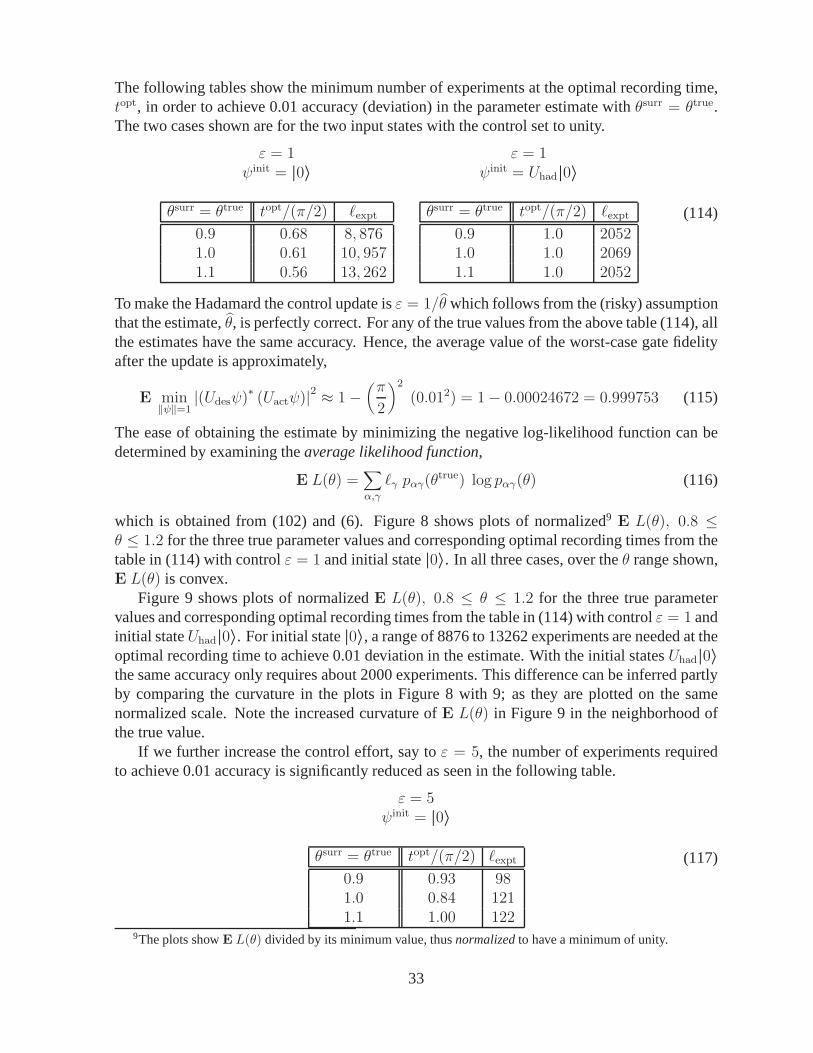
The following tables show the minimum number of experimentsat the optimal recording time,topt, in order to achieve 0.01 accuracy (deviation) in the parameter estimate withθsurr = θtrue.The two cases shown are for the two input states with the control set to unity.

ε = 1ψinit = |0〉

θsurr = θtrue topt/(π/2) ℓexpt

0.9 0.68 8, 8761.0 0.61 10, 9571.1 0.56 13, 262

ε = 1ψinit = Uhad|0〉

θsurr = θtrue topt/(π/2) ℓexpt

0.9 1.0 20521.0 1.0 20691.1 1.0 2052

(114)

To make the Hadamard the control update isε = 1/θ which follows from the (risky) assumptionthat the estimate,θ, is perfectly correct. For any of the true values from the above table (114), allthe estimates have the same accuracy. Hence, the average value of the worst-case gate fidelityafter the update is approximately,

E min‖ψ‖=1

|(Udesψ)∗ (Uactψ)|2 ≈ 1−

(π

2

)2

(0.012) = 1− 0.00024672 = 0.999753 (115)

The ease of obtaining the estimate by minimizing the negative log-likelihood function can bedetermined by examining theaverage likelihood function,

E L(θ) =∑

α,γ

ℓγ pαγ(θtrue) log pαγ(θ) (116)

which is obtained from (102) and (6). Figure 8 shows plots of normalized9 E L(θ), 0.8 ≤θ ≤ 1.2 for the three true parameter values and corresponding optimal recording times from thetable in (114) with controlε = 1 and initial state|0〉. In all three cases, over theθ range shown,E L(θ) is convex.

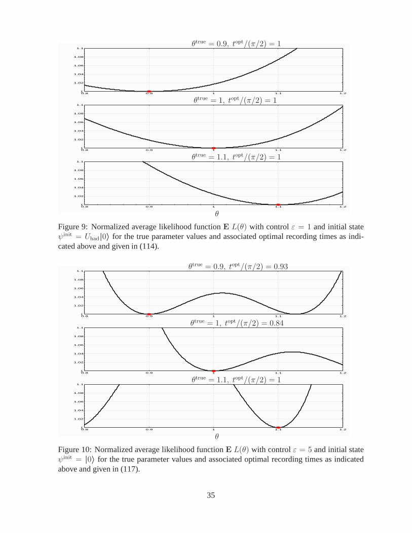
Figure 9 shows plots of normalizedE L(θ), 0.8 ≤ θ ≤ 1.2 for the three true parametervalues and corresponding optimal recording times from the table in (114) with controlε = 1 andinitial stateUhad|0〉. For initial state|0〉, a range of 8876 to 13262 experiments are needed at theoptimal recording time to achieve 0.01 deviation in the estimate. With the initial statesUhad|0〉the same accuracy only requires about 2000 experiments. This difference can be inferred partlyby comparing the curvature in the plots in Figure 8 with 9; as they are plotted on the samenormalized scale. Note the increased curvature ofE L(θ) in Figure 9 in the neighborhood ofthe true value.

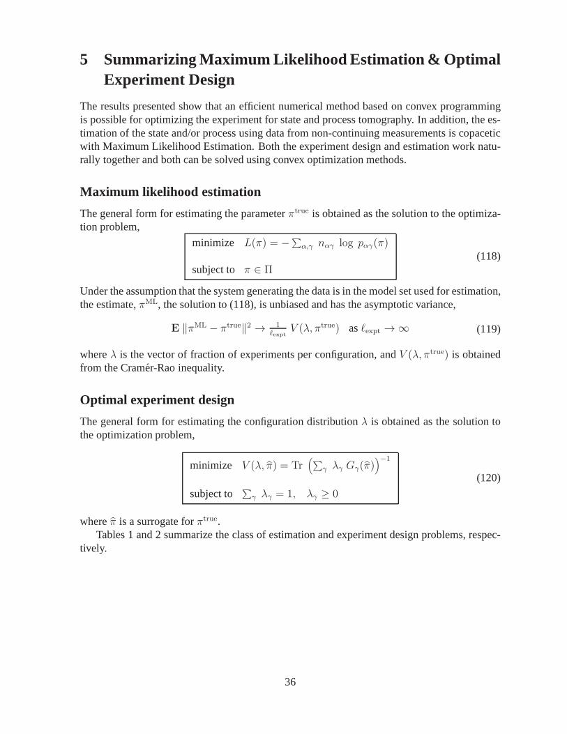
If we further increase the control effort, say toε = 5, the number of experiments requiredto achieve 0.01 accuracy is significantly reduced as seen in the following table.

ε = 5ψinit = |0〉

θsurr = θtrue topt/(π/2) ℓexpt

0.9 0.93 981.0 0.84 1211.1 1.00 122

(117)

9The plots showE L(θ) divided by its minimum value, thusnormalizedto have a minimum of unity.

33

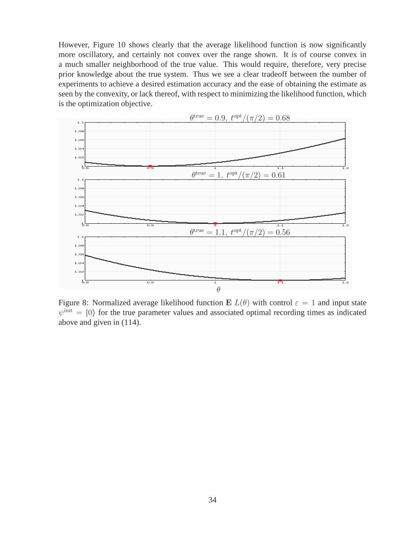
However, Figure 10 shows clearly that the average likelihood function is now significantlymore oscillatory, and certainly not convex over the range shown. It is of course convex ina much smaller neighborhood of the true value. This would require, therefore, very preciseprior knowledge about the true system. Thus we see a clear tradeoff between the number ofexperiments to achieve a desired estimation accuracy and the ease of obtaining the estimate asseen by the convexity, or lack thereof, with respect to minimizing the likelihood function, whichis the optimization objective.

0.9 1 1.10.8 1.2

1.02

1.04

1.06

1.08

1

1.1

0.9 1 1.10.8 1.2

1.02

1.04

1.06

1.08

1

1.1

0.9 1 1.10.8 1.2

1.02

1.04

1.06

1.08

1

1.1

PSfrag replacements

γλoptpure, no noiseλoptpure, yes noiseλoptmixd, no noiseλoptmixd, yes noise

γλopt for ρpure ⊗ ρpureλopt for ρpure ⊗ ρmixd

λopt for ρmixd ⊗ ρmixd

γ

λopt

θ

θtrue = 0.9, topt/(π/2) = 0.68

θtrue = 1, topt/(π/2) = 0.61

θtrue = 1.1, topt/(π/2) = 0.56

Figure 8: Normalized average likelihood functionE L(θ) with controlε = 1 and input stateψinit = |0〉 for the true parameter values and associated optimal recording times as indicatedabove and given in (114).

34

0.9 1 1.10.8 1.2

1.02

1.04

1.06

1.08

1

1.1

0.9 1 1.10.8 1.2

1.02

1.04

1.06

1.08

1

1.1

0.9 1 1.10.8 1.2

1.02

1.04

1.06

1.08

1

1.1

PSfrag replacements

γλoptpure, no noiseλoptpure, yes noiseλoptmixd, no noiseλoptmixd, yes noise

γλopt for ρpure ⊗ ρpureλopt for ρpure ⊗ ρmixd

λopt for ρmixd ⊗ ρmixd

γ

λopt

θ

θtrue = 0.9, topt/(π/2) = 0.68θtrue = 1, topt/(π/2) = 0.61

θtrue = 1.1, topt/(π/2) = 0.56

θ

θtrue = 0.9, topt/(π/2) = 1

θtrue = 1, topt/(π/2) = 1

θtrue = 1.1, topt/(π/2) = 1

Figure 9: Normalized average likelihood functionE L(θ) with controlε = 1 and initial stateψinit = Uhad|0〉 for the true parameter values and associated optimal recording times as indi-cated above and given in (114).

0.9 1 1.10.8 1.2

1.02

1.04

1.06

1.08

1

1.1

0.9 1 1.10.8 1.2

1.02

1.04

1.06

1.08

1

1.1

0.9 1 1.10.8 1.2

1.02

1.04

1.06

1.08

1

1.1

PSfrag replacements

γλoptpure, no noiseλoptpure, yes noiseλoptmixd, no noiseλoptmixd, yes noise

γλopt for ρpure ⊗ ρpureλopt for ρpure ⊗ ρmixd

λopt for ρmixd ⊗ ρmixd

γ

λopt

θ

θtrue = 0.9, topt/(π/2) = 0.68θtrue = 1, topt/(π/2) = 0.61

θtrue = 1.1, topt/(π/2) = 0.56

θ

θtrue = 0.9, topt/(π/2) = 1θtrue = 1, topt/(π/2) = 1

θtrue = 1.1, topt/(π/2) = 1

θ

θtrue = 0.9, topt/(π/2) = 0.93

θtrue = 1, topt/(π/2) = 0.84

θtrue = 1.1, topt/(π/2) = 1

Figure 10: Normalized average likelihood functionE L(θ) with controlε = 5 and initial stateψinit = |0〉 for the true parameter values and associated optimal recording times as indicatedabove and given in (117).

35

5 Summarizing Maximum Likelihood Estimation & OptimalExperiment Design

The results presented show that an efficient numerical method based on convex programmingis possible for optimizing the experiment for state and process tomography. In addition, the es-timation of the state and/or process using data from non-continuing measurements is copaceticwith Maximum Likelihood Estimation. Both the experiment design and estimation work natu-rally together and both can be solved using convex optimization methods.

Maximum likelihood estimation

The general form for estimating the parameterπtrue is obtained as the solution to the optimiza-tion problem,

minimize L(π) = −∑α,γ nαγ log pαγ(π)

subject to π ∈ Π(118)

Under the assumption that the system generating the data is in the model set used for estimation,the estimate,πML, the solution to (118), is unbiased and has the asymptotic variance,

E ‖πML − πtrue‖2 → 1ℓexpt

V (λ, πtrue) asℓexpt → ∞ (119)

whereλ is the vector of fraction of experiments per configuration, andV (λ, πtrue) is obtainedfrom the Cramer-Rao inequality.

Optimal experiment design

The general form for estimating the configuration distribution λ is obtained as the solution tothe optimization problem,

minimize V (λ, π) = Tr(∑

γ λγ Gγ(π))−1

subject to∑γ λγ = 1, λγ ≥ 0

(120)

whereπ is a surrogate forπtrue.Tables 1 and 2 summarize the class of estimation and experiment design problems, respec-

tively.

36

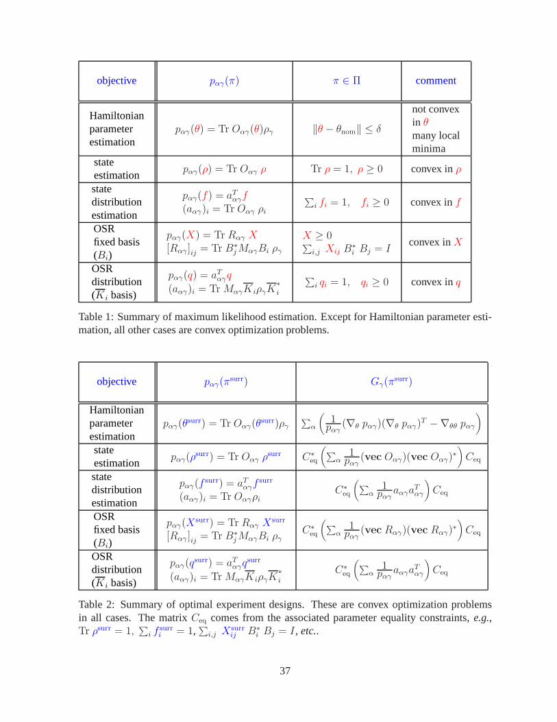
objective pαγ(π) π ∈ Π comment

Hamiltonianparameterestimation

pαγ(θ) = Tr Oαγ(θ)ργ ‖θ − θnom‖ ≤ δ

not convexin θmany localminima

stateestimation

pαγ(ρ) = Tr Oαγ ρ Tr ρ = 1, ρ ≥ 0 convex inρ

statedistributionestimation

pαγ(f) = aTαγf(aαγ)i = Tr Oαγ ρi

∑i fi = 1, fi ≥ 0 convex inf

OSRfixed basis(Bi)

pαγ(X) = Tr Rαγ X[Rαγ ]ij = Tr B∗

jMαγBi ργ

X ≥ 0∑i,j Xij B

∗i Bj = I

convex inX

OSRdistribution(Ki basis)

pαγ(q) = aTαγq

(aαγ)i = TrMαγKiργK∗i

∑i qi = 1, qi ≥ 0 convex inq

Table 1: Summary of maximum likelihood estimation. Except for Hamiltonian parameter esti-mation, all other cases are convex optimization problems.

objective pαγ(πsurr) Gγ(π

surr)

Hamiltonianparameterestimation

pαγ(θsurr) = Tr Oαγ(θ

surr)ργ∑α

(1pαγ

(∇θ pαγ)(∇θ pαγ)T −∇θθ pαγ

)

stateestimation

pαγ(ρsurr) = Tr Oαγ ρ

surr C∗eq

(∑α

1pαγ (vec Oαγ)(vec Oαγ)

∗)Ceq

statedistributionestimation

pαγ(fsurr) = aTαγf

surr

(aαγ)i = Tr OαγρiC∗

eq

(∑α

1pαγ aαγa

Tαγ

)Ceq

OSRfixed basis(Bi)

pαγ(Xsurr) = Tr Rαγ X

surr

[Rαγ ]ij = Tr B∗jMαγBi ργ

C∗eq

(∑α

1pαγ

(vec Rαγ)(vec Rαγ)∗)Ceq

OSRdistribution(Ki basis)

pαγ(qsurr) = aTαγq

surr

(aαγ)i = TrMαγKiργK∗i

C∗eq

(∑α

1pαγ aαγa

Tαγ

)Ceq

Table 2: Summary of optimal experiment designs. These are convex optimization problemsin all cases. The matrixCeq comes from the associated parameter equality constraints,e.g.,Tr ρsurr = 1,

∑i f

surri = 1,

∑i,j X

surrij B∗

i Bj = I, etc..

37

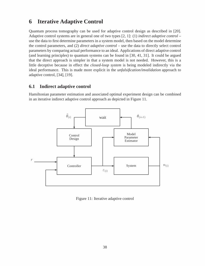
6 Iterative Adaptive Control

Quantum process tomography can be used for adaptive controldesign as described in [20].Adaptive control systems are in general one of two types [2, 1]: (1) indirect adaptive control–use the data to first determine parameters in a system model, then based on the model determinethe control parameters, and (2)direct adaptive control– use the data to directly select controlparameters by comparing actual performance to an ideal. Applications of direct adaptive control(and learning principles) to quantum systems can be found in[30, 41, 31]. It could be arguedthat the direct approach is simpler in that a system model is not needed. However, this is alittle deceptive because in effect theclosed-loop systemis being modeled indirectly via theideal performance. This is made more explicit in theunfalsification/invalidationapproach toadaptive control, [34], [19].

6.1 Indirect adaptive control

Hamiltonian parameter estimation and associated optimal experiment design can be combinedin an iterative indirect adaptive control approach as depicted in Figure 11.

Controller System

ControlDesign

ModelParameterEstimator

r

wait θ(i+1)θ(i)

ε(i)

n(i)

Figure 11: Iterative adaptive control

38

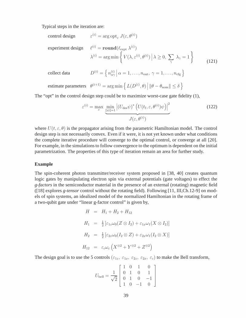
Typical steps in the iteration are:

control design ε(i) = arg optε J(ε, θ(i))

experiment design ℓ(i) = round(ℓexpt λ(i))

λ(i) = argmin

V (λ, ε(i), θ(i))

∣∣∣λ ≥ 0,∑

γ

λγ = 1

collect data D(i) =n(i)αγ

∣∣∣α = 1, . . . , nout, γ = 1, . . . , ncfg

estimate parametersθ(i+1) = argminL(D(i), θ)

∣∣∣ ‖θ − θnom‖ ≤ δ

(121)

The “opt” in the control design step could be to maximize worst-case gate fidelity (1),

ε(i) = maxε

min‖ψ‖=1

∣∣∣(Udesψ)∗ (U(tf , ε, θ(i))ψ

)∣∣∣2

︸ ︷︷ ︸J(ε, θ(i))

(122)

whereU(t, ε, θ) is the propagator arising from the parametric Hamiltonian model. The controldesign step is not necessarily convex. Even if it were, it is not yet known under what conditionsthe complete iterative procedure will converge to the optimal control, or converge at all [20].For example, in the simulations to follow convergence to theoptimum is dependent on the initialparametrization. The properties of this type of iteration remain an area for further study.

Example

The spin-coherent photon transmitter/receiver system proposed in [38, 40] creates quantumlogic gates by manipulating electron spin via external potentials (gate voltages) to effect theg-factorsin the semiconductor material in the presence of an external(rotating) magnetic field([18] exploresg-tensorcontrol without the rotating field). Following [11, III,Ch.12-9] on mod-els of spin systems, an idealized model of the normalized Hamiltonian in the rotating frame ofa two-qubit gate under “linear g-factor control” is given by,

H = H1 +H2 +H12

H1 = 12[ε1zω0(Z ⊗ I2) + ε1xω1(X ⊗ I2)]

H2 = 12[ε2zω0(I2 ⊗ Z) + ε2xω1(I2 ⊗X)]

H12 = εcωc(X⊗2 + Y ⊗2 + Z⊗2

)

The design goal is to use the 5 controls(ε1z, ε1x, ε2z, ε2x, εc) to make the Bell transform,

Ubell =1√2

1 0 1 00 1 0 10 1 0 −11 0 −1 0

39

One of the many possible decompositions of the Bell transform is the following:

Ubell = (Uhad ⊗ I2)√Uswap (X

−1/2 ⊗X1/2)√Uswap (I2 ⊗X)

Each operation in this sequence uses only the single qubit and swap “gates” produced by simul-taneously pulsing the 5 controls as shown in the following table.

ε1z ε1x ε2z ε2x εc ∆t gate

0 0 0 1 0 πω1

−iI2 ⊗X

0 0 0 0 1 π8ωc

e−iπ8

√Uswap

0 0 0 1 0 π2ω1

e−iπ4 I2 ⊗X1/2

0 1 0 0 0 3π2ω1

e−i3π4 X−1/2 ⊗ I2

0 0 0 0 1 π8ωc

e−iπ8

√Uswap

ωhad

ω0

√2

ωhad

ω1

√2

0 0 0 πωhad

−iUhad ⊗ I2

Figure 12: Pulse control table

The resulting gate at the final time,tf , isUbell to within a scalar phase:

U(tf) = e−iπ4 Ubell, tf =

(3

ω1+

1

4ωc+

1

ωhad

)π

Suppose the only unknown parameter isω1. Consider the following simplified version of (121):

control design ε(i) = ε(ω(i)1 ), tf

(i) = tf(ω(i)1 )

estimation ω(i+1)1 = argmin

ω1

E L(ω1, ε(i))

where the control design functionε(ω(i)1 ) represents the pulse design from the above table, and

where the average likelihood function follows from the description in Section§4.1 with thefollowing parameters:

single initial state ρinit = |0〉〈0| (β = 1)POVM M1 = |0〉〈0|, M2 = |1〉〈1| (nout = 2)sample times eithertf(ω1), (nsa = 1) or tf(ω1)/2, tf(ω1), (nsa = 2)

Using Hamiltonian parameters(ωtrue0 = 1, ωtrue

1 = 0.01, ωtruec = 0.01), Figure 13 shows

E L(ω1, nsa = 1) vs. ω1/ωtruei for sequences of adaptive iterations using the estimateω1

obtained from a local hill climbing algorithm,i.e., the local maximum of the average likelihood

40

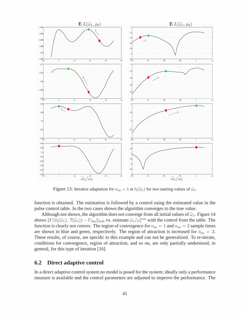
1 1.1 1.2 1.30.9 1.4

-1.39

-1.388

-1.386

-1.384

-1.392

-1.382

1 1.1 1.2 1.30.9 1.4

-1.385

-1.38

-1.375

-1.39

-1.37

1 1.1 1.2 1.30.9 1.4

-1.41

-1.4

-1.39

-1.42

-1.38

1 1.1 1.2 1.30.9 1.4

-1.44

-1.43

-1.42

-1.41

-1.4

-1.39

-1.45

-1.38

PSfrag replacementsγ

λoptpure, no noiseλoptpure, yes noiseλoptmixd, no noiseλoptmixd, yes noise

γλopt for ρpure ⊗ ρpureλopt for ρpure ⊗ ρmixd

λopt for ρmixd ⊗ ρmixdγλopt

θθtrue = 0.9, topt/(π/2) = 0.68θtrue = 1, topt/(π/2) = 0.61

θtrue = 1.1, topt/(π/2) = 0.56

θθtrue = 0.9, topt/(π/2) = 1θtrue = 1, topt/(π/2) = 1

θtrue = 1.1, topt/(π/2) = 1

θθtrue = 0.9, topt/(π/2) = 0.93θtrue = 1, topt/(π/2) = 0.84θtrue = 1.1, topt/(π/2) = 1

E L(ω1, ρ0)

ω1/ω1

0.7 0.8 0.9 10.6 1.1

-2

-1.8

-1.6

-1.4

-1.2

-2.2

-1

0.7 0.8 0.9 10.6 1.1

-1.8

-1.6

-1.4

-1.2

-2

-1

0.7 0.8 0.9 10.6 1.1

-2.5

-2

-1.5

-3

-1

0.7 0.8 0.9 10.6 1.1

-3.5

-3

-2.5

-2

-1.5

-4

-1

PSfrag replacementsγ

λoptpure, no noiseλoptpure, yes noiseλoptmixd, no noiseλoptmixd, yes noise

γλopt for ρpure ⊗ ρpureλopt for ρpure ⊗ ρmixd

λopt for ρmixd ⊗ ρmixdγλopt

θθtrue = 0.9, topt/(π/2) = 0.68θtrue = 1, topt/(π/2) = 0.61

θtrue = 1.1, topt/(π/2) = 0.56

θθtrue = 0.9, topt/(π/2) = 1θtrue = 1, topt/(π/2) = 1

θtrue = 1.1, topt/(π/2) = 1

θθtrue = 0.9, topt/(π/2) = 0.93θtrue = 1, topt/(π/2) = 0.84θtrue = 1.1, topt/(π/2) = 1

E L(ω1, ρ0)

ω1/ω1

Figure 13:Iterative adaptation fornsa = 1 at tf(ω1) for two starting values ofω1.

function is obtained. The estimation is followed by a control using the estimated value in thepulse control table. In the two cases shown the algorithm converges to the true value.

Although not shown, the algorithm does not converge from allinitial values ofω1. Figure 14shows‖U(tf(ω1), ε(ω1))−Udes‖frob vs. estimateω1/ω

true1 with the control from the table. The

function is clearly not convex. The region of convergence for nsa = 1 andnsa = 2 sample timesare shown in blue and green, respectively. The region of attraction is increased fornsa = 2.These results, of course, are specific to this example and cannot be generalized. To re-iterate,conditions for convergence, region of attraction, and so on, are only partially understood, ingeneral, for this type of iteration [16].

6.2 Direct adaptive control

In a direct adaptive control system no model is posed for the system; ideally only a performancemeasure is available and the control parameters are adjusted to improve the performance. The

41

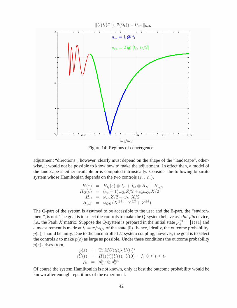
‖U(tf(ω1), ε(ω1))− Udes‖frob

0.5 1 1.5 20 2.5

1

2

3

0

4

PSfrag replacementsγ

λoptpure, no noiseλoptpure, yes noiseλoptmixd, no noiseλoptmixd, yes noise

γλopt for ρpure ⊗ ρpureλopt for ρpure ⊗ ρmixd

λopt for ρmixd ⊗ ρmixdγλopt

θθtrue = 0.9, topt/(π/2) = 0.68θtrue = 1, topt/(π/2) = 0.61

θtrue = 1.1, topt/(π/2) = 0.56

θθtrue = 0.9, topt/(π/2) = 1θtrue = 1, topt/(π/2) = 1

θtrue = 1.1, topt/(π/2) = 1

θθtrue = 0.9, topt/(π/2) = 0.93θtrue = 1, topt/(π/2) = 0.84θtrue = 1.1, topt/(π/2) = 1

E L(ω1, ρ0)ω1/ω1

ω1/ω1

nsa = 1 @ tf

nsa = 2 @ [tf , tf/2]

Figure 14: Regions of convergence.

adjustment “directions”, however, clearly must depend on the shape of the “landscape”, other-wise, it would not be possible to know how to make the adjustment. In effect then, a model ofthe landscape is either available or is computed intrinsically. Consider the following bipartitesystem whose Hamiltonian depends on the two controls(εz, εx).

H(ε) = HQ(ε)⊗ IE + IQ ⊗HE +HQE

HQ(ε) = (εz − 1)ωQzZ/2 + εxωQxX/2HE = ωEzZ/2 + ωExX/2HQE = ωQE (X⊗2 + Y ⊗2 + Z⊗2)

The Q-part of the system is assumed to be accessible to the user and the E-part, the “environ-ment”, is not. The goal is to select the controls to make the Q-system behave as abit-flip device,i.e., the PauliX matrix. Suppose the Q-system is prepared in the initial stateρinitQ = |1〉〈1| anda measurement is made attf = π/ωQx of the state|0〉. hence, ideally, the outcome probability,p(ε), should be unity. Due to the uncontrolledE-system coupling, however, the goal is to selectthe controlsε to makep(ε) as large as possible. Under these conditions the outcome probabilityp(ε) arises from,

p(ε) = TrMU(tf)ρ0U(tf)∗

iU(t) = H(ε(t))U(t), U(0) = I, 0 ≤ t ≤ tfρ0 = ρinitQ ⊗ ρinitE

Of course the system Hamiltonian is not known, only at best the outcome probability would beknown after enough repetitions of the experiment.

42

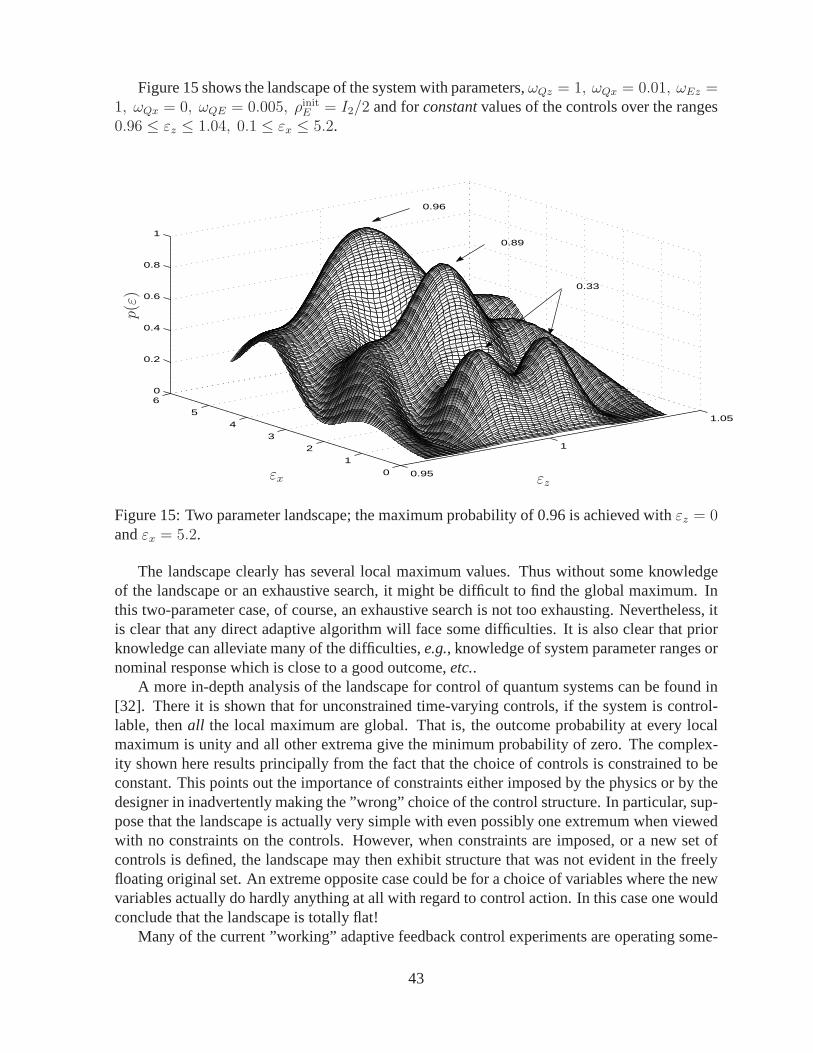
Figure 15 shows the landscape of the system with parameters,ωQz = 1, ωQx = 0.01, ωEz =1, ωQx = 0, ωQE = 0.005, ρinitE = I2/2 and forconstantvalues of the controls over the ranges0.96 ≤ εz ≤ 1.04, 0.1 ≤ εx ≤ 5.2.

0.95

1

1.05

0

1

2

3

4

5

60

0.2

0.4

0.6

0.8

1

0.96

0.89

0.33

PSfrag replacements

γλoptpure, no noiseλoptpure, yes noiseλoptmixd, no noiseλoptmixd, yes noise

γλopt for ρpure ⊗ ρpureλopt for ρpure ⊗ ρmixd

λopt for ρmixd ⊗ ρmixd

γ

λopt

θ

θtrue = 0.9, topt/(π/2) = 0.68θtrue = 1, topt/(π/2) = 0.61

θtrue = 1.1, topt/(π/2) = 0.56

θ

θtrue = 0.9, topt/(π/2) = 1θtrue = 1, topt/(π/2) = 1

θtrue = 1.1, topt/(π/2) = 1

θ

θtrue = 0.9, topt/(π/2) = 0.93θtrue = 1, topt/(π/2) = 0.84θtrue = 1.1, topt/(π/2) = 1

E L(ω1, ρ0)ω1/ω1

ω1/ω1

nsa = 1 @ tfnsa = 2 @ [tf , tf/2]

p(ε)

εzεx

Figure 15: Two parameter landscape; the maximum probability of 0.96 is achieved withεz = 0andεx = 5.2.

The landscape clearly has several local maximum values. Thus without some knowledgeof the landscape or an exhaustive search, it might be difficult to find the global maximum. Inthis two-parameter case, of course, an exhaustive search isnot too exhausting. Nevertheless, itis clear that any direct adaptive algorithm will face some difficulties. It is also clear that priorknowledge can alleviate many of the difficulties,e.g., knowledge of system parameter ranges ornominal response which is close to a good outcome,etc..

A more in-depth analysis of the landscape for control of quantum systems can be found in[32]. There it is shown that for unconstrained time-varyingcontrols, if the system is control-lable, thenall the local maximum are global. That is, the outcome probability at every localmaximum is unity and all other extrema give the minimum probability of zero. The complex-ity shown here results principally from the fact that the choice of controls is constrained to beconstant. This points out the importance of constraints either imposed by the physics or by thedesigner in inadvertently making the ”wrong” choice of the control structure. In particular, sup-pose that the landscape is actually very simple with even possibly one extremum when viewedwith no constraints on the controls. However, when constraints are imposed, or a new set ofcontrols is defined, the landscape may then exhibit structure that was not evident in the freelyfloating original set. An extreme opposite case could be for achoice of variables where the newvariables actually do hardly anything at all with regard to control action. In this case one wouldconclude that the landscape is totally flat!

Many of the current ”working” adaptive feedback control experiments are operating some-

43

where between these two extremes, ranging from having highly constrained knobs to the totallywrong knobs. This comment comes from the observation that physical effects spanning a dy-namic range in quantum wavelength of about107 are being controlled by a single type of laser,i.e., the Ti:Sapphire laser, working over a range of about 1-10 onthat scale. That is, a domainin laser wavelength of 10 (in some units) is split up into about 100 small pieces as controls, andthose very narrow controls manage everything over a huge dynamic range. The fact that theexperiments work at all is rather amazing. A guess is that an examination of the landscapes willshow considerable detail, much of which is likely false structures arising from having highlyconstrained controls. From a positive perspective, as morebandwidth becomes available thecontrol landscape will become less complicated and more regular in the sense that more of thelocal optimum values will provide performance close to the global optimum.

A Appendix

A.1 Worst-case gate fidelity

From the definition of worst-case fidelity (1),

|(Udesψ)∗ (Uactψ)|2 = |ψ∗(U∗

desUact)ψ|2= |(V ∗ψ)∗Ω(V ∗ψ)|2= |∑n

k=1 ωk |xk|2|2

= |∑nk=1 ωk zk|2

where the last three lines follow directly from (i) the eigenvalue decomposition of the unitary:U∗desUact = V ΩV ∗, V ∗V = In, Ω = diag(ω1 · · · ωn), |ωk| = 1, (ii) definingx = V ∗ψ ∈ Cn,

and (iii) definingzk = |xk|2 ∈ R. Using the definitions of the vectors(a, b) in (2) gives,

|(Udesψ)∗ (Uactψ)|2 =

∣∣∣∣∣

n∑

k=1

(ak + ibk) zk

∣∣∣∣∣

2

= zT (aaT + bbT )z

The QP follows from the relations:

‖ψ‖ = 1 ⇔ ‖x = V ∗ψ‖ = 1 ⇔∑

k

(zk = |xk|2) = 1, zk ≥ 0

A.2 Cramer-Rao Inequality

The following is the classical form of the Cramer-Rao Inequality.

Cramer-Rao Inequality[8]Let θ0 ∈ Rp be the true parameter to be estimated from a data setD. LetL(D, θ0)be the true negative log-likelihood function of the system generating the data. Letθ ∈ Rp be an unbiased estimate ofθ0, i.e., E θ = θ0. Then, the covariance of theestimate,

covθ = E(θ − θ0

) (θ − θ0

)T(123)

44

satisfies the matrix inequality,[cov θ II F (θ0)

]≥ 0 (124)

whereF (θ0) is theFisher information matrix,

F (θ0) = E ∇θθL(D, θ)

∣∣∣∣θ=θ0

(125)

If F (θ0) > 0, then (124) is equivalent to,

covθ ≥ F (θ0)−1 (126)

This famous theorem states the for any unbiased estimator, the covariance of the estimate satis-fies the inequality (124), or equivalently (126), provided the Fisher matrix is invertible. Usuallyonly (126) is given as the theorem: the minimum covariance ofthe estimate is given by theinverse of the Fisher information matrix. The power of the result (124) is that it is independentof how the estimate is obtained. The lower bound only depends on themodel structure, theexperiment design, and the information in the data.

A.3 Derivation of (28)

Define the vectorsr, aαγ ∈ Cn2

as,

r = vec ρ, aαγ = vec Oαγ

Thenpαγ = Tr Oαγρ = a∗αγr

andTr ρ = 1 ⇔ bT r = 1, b = vec In

The next step eliminates the equality constraintbT r = 1 reducing then2 unknowns inr ton2 − 1. SincebT b = n, the SVD ofb is,

b =W

[ √n

0n2−n

]

with unitaryW ∈ Rn2×n2

, PartitionW = [c Ceq] with Ceq ∈ Rn2×n2−1. Then allr satisfyingbT r = 1 are given by

r = c/√n + Ceqz

for all z ∈ Cn2−1. The likelihood function with the equality constraint (Tr ρ = 1 or bT r = 1)eliminated is then a function only ofz,

L(D, z) = −∑

α,γ

nαγ log(c/√n + Ceqz)

45

To obtain the Cramer-Rao bound, we first compute,

∇zzL(D, z) =∑

α,γ

nαγpαγ(z)2

(CTeqaαγ)(C

Teqaαγ)

∗

Using (6),E nαγ = ℓγpαγ(ρtrue), ρtrue = c/

√n + Ceqz

true, and hence the Fisher informationmatrix is, with respect toz,

F = E L(D, z = ztrue)

=∑

α,γ

ℓγpαγ(ρtrue)

(CTeqaαγ)(C

Teqaαγ)

∗

= G(ℓ, ρtrue)

where the last line comes from the definition ofG(ℓ, ρtrue) in (29). Letr = c/√n+Ceqz be an

unbiased estimate ofrtrue. Thus,

cov r = Ceqcov z CTeq ≥ CeqF

−1CTeq

Usingvar ρ = var r = Tr cov r and the fact thatW is unitary, and hence,CTeqCeq = In2−1,

we get,var ρ ≥ Tr CeqF

−1CTeq = Tr F−1

which is the final result (28)-(29).

A.4 Derivation of (80)

Definex, rαγ ∈ Cn4

as,x = vec X, rαγ = vec Rαγ

The likelihood function in (75) can then be written as,

L(D, x) = −∑

α,γ

nαγ log r∗αγx

and the equality constraint in (75) becomes,

Ax = vec In, A = [a1 · · · an4] ∈ Cn2×n4

with ak = vec(B∗iBj) ∈ Cn2

for k = i+(j−1)n2, i, j = 1, . . . , n2. Perform the singular valuedecompositionA = U [S 0]W ∗, W = [C Ceq] with C ∈ Cn2×n2

, Ceq ∈ Cn2×n4−n2

as given in(82). From the definition of the basis functions (69) it follows thatS =

√n In2 . Observe also

that the columns ofCeq are a basis for the nullspace ofA. Hence allx satisfying the equalityconstraint are given by,

x = x+ Ceqz, ∀z with x = (1/√n)CU∗vec In

The likelihood function with the equality constraint (Ax = vec In) eliminated is then a functiononly of z,

L = −∑

α,γ

nαγ log(x+ Ceqz)

This is exactly the same form of the likelihood function in§A.3 after the single equality con-straint there is eliminated. Hence, to obtain the Cramer-Rao bound (80) repeat,mutatis mutan-dis, the procedure in§A.3.

46

References

[1] B.D.O. Anderson, R.R. Bitmead, Jr. C.R. Johnson, P.V. Kokotovic, R.L. Kosut, I.M.Y.Mareels, L. Praly, and B.D. Riedle.Stability of Adaptive Systems: Passivity and AveragingAnalysis. MIT Press, 1986.

[2] K. J. Astrom and B. Wittenmark.Adaptive Control. Addison-Wesley,, 1995.

[3] K. Audenaert and B. De Moor. Optimizing completely positive maps using semidefiniteprogramming.Phys. Rev. A, 65, 2003.

[4] K. Banaszek. Reconstruction of photon distribution with positivity constraints.acta phys-ica slovaca, 48(3):185–190, June 1998.

[5] S. Boyd and L. Vandenberghe.Convex Optimization. Cambridge University Press, 2004.also available atwww.stanford.edu/∼boyd/cvxbook.html.

[6] A. M. Childs, J. Preskill, and J. Renes. Quantum information and precision measurement.J.Mod.Opt., 47:155–176, 2000. e-Print Archive: quant-ph/9904021.

[7] I.L. Chuang and M.A. Nielsen. Prescription for experimental determination of the dynam-ics of a quantum black box.J. Mod. Opt., 44:2455–2467, 1997.

[8] H. Cramer.Mathematical Methods of Statistics. Princeton Press, 1946.

[9] Y. C. Eldar, A. Megretski, and G. C. Verghese. Designing optimal quantum detectors viasemidefinite programming.IEEE Trans. Inform. Theory, 49:1017–1012, Apr. 2003.

[10] M. Fazel, H. Hindi, and S. P. Boyd. A rank minimization heuristic with application to min-imum order system approximation.Proc. American Control Conference, 6:4734–4739,June 2001.

[11] R. P. Feynman, R. B. Leighton, and M. Sands.The Feynman Lectures on Physics.Addison-Wesley, 1963-1965.

[12] J. M. Geremia and H. Rabitz. Teaching lasers to optimally identify molecular hamiltoni-ans.Phys. Rev. Lett., 89 263902, 2002.

[13] A. Gilchrist, N. K. Langford, and M. A. Nielsen. Distance measures to compare real andideal quantum processes.arXiv quant-ph/0408063, August 2004.

[14] G. H. Golub and C. F. Van Loan.Matrix Computations. Johns Hopkins University Press,1983.

[15] W. P. Grice and I. A. Walmsley. Homodyne detection in a photon counting application.Journal of Modern Optics, 1996.

[16] H. Hjalmarsson, M. Gevers, and F. De Bruyne. For model-based control design, closedloop identification gives better performance.Automatica, 32(12):1659–1673, December1996.

47

[17] D. F. V. James, P. G. Kwiat, W. J. Munroe, and A. G. White. Measurement of qubits.Phys.Rev. A, 64 052312, 2001.

[18] Y. Kato, R. C. Myers, D. C. Driscoll, A. C. Gossard, J. Levy, and D. D. Awschalom. Gi-gahertz electron spin manipulation using voltage controlled g-tensor modulation.Science,299, 2003.

[19] R. L. Kosut. Iterative adaptive control: Windsurfing with confidence. In G. Goodwin, edi-tor,Model Identification and Adaptive Control: From Windsurfingto Telecommunications.Springer-Verlag, 2001.

[20] R. L. Kosut, H. Rabitz, and I. A. Walmsley. Maximum likelihood identification of quantumsystems for control design.13th IFAC Symposium on System Identification, 27-29 August2003. Rotterdam, The Netherlands.

[21] R. L. Kosut, I. A. Walmsley, Y. Eldar, and H. Rabitz. Quantum state detector : optimalworst-case a posteriori performance.arXiv:quant-ph/0403150, March 2004.

[22] L. Ljung. System Identification: Theory for the User. Prentice-Hall, first edition edition,1987.

[23] J. Lofberg. Yalmip: a matlab toolbox for rapid prototyping of opti-mization problems. Automatic Control Laboratory, ETH Zurich, 2004.http://control.ee.ethz.ch/ joloef/yalmip.msql.

[24] H. Mabuchi. Dynamical identification of open quantum systems. Quantum Semiclass.Opt., 8(6), December 1996.

[25] A. Mitra and H. Rabitz. Identifying mechanisms in the control of quantum dynamicsthrough hamiltonian encoding.Phys. Rev. A, 67 033407:1–16, 2003.

[26] Y. Nesterov and A. Nemirovskii.Interior-Point Polynomial Methods in Convex Program-ming. Society for Industrial and Applied Mathematics, 1994.

[27] M. A. Nielsen and I. L. Chuang.Quantum Computation and Quantum Information. Cam-bridge, 2000.

[28] A. Papoulis. Probability, Random Variables, and Stochastic Processes. McGraw-Hill,1965.

[29] M. G. A. Paris, G. M. D’Ariano, and M. F. Sacchi. Maximum likelihood method inquantum estimation.arXiv: quant-ph/ 0101071 v1, 16 Jan 2001.

[30] M.Q. Phan and H. Rabitz. Learning control of quantum-mechanical systems by laboratoryidentification of effective input-output maps.Chem. Phys., 217:389–400, 1997.

[31] M.Q. Phan and H. Rabitz. A self-guided algorithm for learning control of quantum-mechanical systems.J. Chem. Phys., 110:34–41, 1999.

48

[32] H. Rabitz, M. Hsieh, and C. Rosenthal. Quantum optimally controlled transition land-scapes.Science, 303, 2004.

[33] M. F. Sacchi. Maximum-likelihood reconstruction of completely positive maps.Phys.Rev. A, 63 054104, April 2001.

[34] M. G. Safonov and T. C. Tsao. The unfalsified control concept and learning.IEEE Trans.Aut. Contr., 42(6):843–847, June 1997.

[35] K. C. Toh, R. H. Tutuncu, and M. J. Todd. Sdpt3: Matlab software for semidefinite-quadratic-linear programming. 2004. http://www.math.nus.edu.sg/ mattohkc/sdpt3.html.

[36] L. Vandenberghe, S. Boyd, and S.-P. Wu. Determinant maximization with linear matrixinequality constraints.SIAM Journal on Matrix Analysis and Applications, 19(2):499–533, 1998.

[37] F. Verstraete, A. C. Doherty, and H. Mabuchi. Sensitivity optimization in quantum param-eter estimation.Phys. Rev. A, 64(032111), 2001. quant-ph/0104116 v1, 24 Apr 2001.

[38] R. Vrijen, E. Yablonovitch, K.Wang, H. W. Jiang, A. Balandin, V. Roychowdhury, T.Mor,and D. DiVincenzo. Electron-spin-resonance transistors for quantum computing in silicon-germanium heterostructures.Physical Review A, 62:1050–2947, 2000.

[39] I. A. Walmsley and L. Waxer. Emission tomography for quantum state measurement inmatter.Phys. B: At. Mol. Opt. Phys., 31:1825–1863, 1998.

[40] E. Yablonovitch, H. W. Jiang, H. Kosaka, H. D. Robinson,D. S. Rao, and T. Szkopek. Op-toelectronic quantum telecommunications based on spins insemiconductors.Proceedingsof the IEEE, 91(5), May 2003.

[41] W. Zhu and H. Rabitz. Uniform rapidly convergent algorithm for quantum optimal controlof objectives with a positive semi-definite hessian matrix.Phys. Rev. A, 58, 1998.

49