Embed Size (px)
Citation preview

Journal of Soft Computing in Civil Engineering 2-3 (2018) 50-71
SCCE is an open access journal under the CC BY license (http://creativecommons.org/licenses/BY/4.0/)
Contents lists available at SCCE
Journal of Soft Computing in Civil Engineering
Journal homepage: http://www.jsoftcivil.com/
Artificial Neural Networks Prediction of Compaction
Characteristics of Black Cotton Soil Stabilized with Cement Kiln
Dust
A. B. Salahudeen1*
, T. S. Ijimdiya2, A. O. Eberemu
2 and K. J. Osinubi
2
1. Samaru College of Agriculture, Division of Agricultural Colleges, Ahmadu Bello University, Zaria, Nigeria
2. Department of Civil Engineering, Ahmadu Bello University, Zaria, Nigeria
Corresponding author: [email protected]
http://dx.doi.org/10.22115/SCCE.2018.128634.1059
ARTICLE INFO
ABSTRACT
Article history:
Received: 25 April 2018
Revised: 23 May 2018
Accepted: 24 May 2018
Artificial neural networks (ANNs) that have been
successfully applied to structural and most other disciplines
of civil engineering is yet to be extended to soil stabilization
aspect of geotechnical engineering. As such, this study aimed
at applying the ANNs as a soft computing approach that
were trained with the feed forward back-propagation
algorithm, for the simulation of optimum moisture content
(OMC) and maximum dry density (MDD) of cement kiln
dust-stabilized black cotton soil. Ten input and two output
data set were used for the ANN model development. The
mean squared error (MSE) and R-value were used as
yardstick and criterions for acceptability of performance. In
the neural network development, NN 10-5-1 and NN 10-7-1
respectively for OMC and MDD that gave the lowest MSE
value and the highest R-value were used in the hidden layer
of the networks architecture and performed satisfactorily. For
the normalized data used in training, testing and validating
the neural network, the performance of the simulated
network was satisfactory having R values of 0.983 and
0.9884 for the OMC and MDD, respectively. These values
met the minimum criteria of 0.8 conventionally
recommended for strong correlation condition. All the
obtained simulation results are satisfactory, and a strong
correlation was observed between the experimental OMC
and MDD values as obtained by laboratory tests and the
predicted values using ANN.
Keywords:
Artificial neural networks,
Black cotton soil,
Cement kiln dust,
Maximum dry density,
Optimum moisture content,
Soil stabilization.

51 A. B. Salahudeen et al./ Journal of Soft Computing in Civil Engineering 2-3 (2018) 50-71
1. Introduction
The optimum moisture content (OMC) and maximum dry density (MDD) of soils are
phenomena whose study is unavoidably vital in field and laboratory soil compaction works. Soil
compaction which is the process of densification of soil by pore air removal requires the
application of mechanical energy to achieve. The degree of compaction of soil is determined in
terms of the dry density of the soil. The application of water to the soil in the process of
compaction makes the water acts as a medium for softening the soil particles. This makes the soil
particles slip over each other than relocate to a more densely packed position. The dry density
first increases after compaction with an increase in water content. As the water content is
gradually increased, if the used compaction effort is maintained, the weight of the soil solids per
unit volume also increases gradually. Beyond a certain water content, a further increase in the
water content causes a decrease in the dry density. This phenomenon is as a result of the water
occupying the pore spaces that supposed to have been occupied by the solid particles. The water
content at which the maximum dry density (MDD) is attained, is generally referred to as the
optimum moisture content (OMC).
Artificial Neural Networks (ANNs), which is a form of artificial intelligence, that in its
architecture tries to mimic the biology of the human brain and nervous system was used in this
study. The important component of this simulation is the novel structure of the information
processing system which consists of a huge amount of well-interconnected processing elements
(neurons) focused on solving a particular problem [1-2]. Just as it is the case in human beings,
ANNs also learn by training. An ANN is developed for a distinct application. These applications
include patterns recognition and data classification through a learning process. There are several
types of ANNs with different applications, such as data association, data prediction, data
classification, data conceptualization and data filtering. The most common type of ANN has
three interconnected layers: input, hidden and output. Multi-layer networks make use several
types of learning techniques; the most popular of which is back-propagation [3-5], which is also
employed in this study.
In the last two decades, ANNs have been used in many geotechnical engineering applications.
Shahin et al. [6] have used back-propagation neural networks to predict foundation settlements.
The predicted settlements obtained based on the use of ANNs were compared with those
obtained by three commonly used conventional methods. The study results revealed that ANNs
are a promising method for foundations settlement prediction, as they perform better than the
deterministic methods considered. Kolay et al. [1] made use of ANN programming in predicting
the compressibility characteristics of soft soil settlement in Sarawak, Malaysia. Benali et al.[7]
used ANNs for principal component analysis and predicting capacity of pile based on SPT
results. All these literature are a source of hope for the beneficial use of ANNs in geotechnical
applications.
Black cotton soils (BCS) are expansive soils which are so named due to their mostly dark color
and suitability for growing cotton. BCS is confined to the semi-arid regions of tropical and
temperate climatic zones. They are abundant in regions where the annual evaporation is more
than the precipitation [13]. BCS is common in flat terrains that has poor drainage system [14].
The mineralogy of BCS is dominated by montmorillonite clay mineral which has the
characteristics of high change in volume from dry to wet seasons and vice versa. Deposits of

A. B. Salahudeen et al./ Journal of Soft Computing in Civil Engineering 2-3 (2018) 50-71 52
BCS occupy an estimated area of 104 x 103
km2 in the North-Eastern part of Nigeria. These areas
are generally known with a pattern of cracks during the dry season. These cracks measure up to
70mm wide and over 1m deep and may extend beyond 3m in areas with high deposit [15-16].
The increasing cost of soil stabilizers coupled with the need to reduce the cost of waste disposal
has led to a serious global research focus on the beneficial use of wastes in engineering
applications [8-10]. The safe disposal of wastes from industries needs fast and economic
solutions due to the destructive effect of these materials on our environment and also the health
hazards they constitute [11]. Cement kiln dust (CKD) is a solid highly alkaline waste which is
fine-grained removed from the cement kiln exhaust gas by air pollution control devices of
cement production plants in cement industries. [12].
In this study, standard laboratory procedures were used to determine the properties of natural and
CKD-treated BCS using three compaction energies. The study aimed at using the soil properties
to develop an optimized neural network for the OMC and MDD of natural and CKD-stabilised
black cotton soil using multi-layer networks variety of learning technique of back-propagation in
Artificial Neural Networks (ANNs).
2. Materials and methods
2.1. Materials
2.1.1. Soil
The disturbed BCS samples used herein were obtained from Deba, Gombe State of Nigeria.
2.1.2. Cement Kiln Dust
The CKD used for this study was sourced from Sokoto Cement, Sokoto, Nigeria. The oxide
composition of the BCS and CKD used for this study is shown in Table 1. The only benefit of
including the oxide composition of the materials is to distinguish them from any other materials
that may be used to reproduce the research and results compared since material properties is the
best characteristics to differentiate materials.
Table 1. Oxide composition of black cotton soil (BCS) and cement kiln dust (CKD)
Oxide BCS (%) CKD (%)
CaO 4.53 44.28
SiO2 42.45 7.23
Al2O3 13.19 1.90
Fe2O3 16.75 4.47
MgO - 0.82
MnO 0.62 0.11
TiO2 3.17 0.23
V2O5 0.22 0.03
Cr2O3 0.031 0.02
ZnO - 0.01
K2O 3.03 -
LOI (10000C) 15.34 39.28

53 A. B. Salahudeen et al./ Journal of Soft Computing in Civil Engineering 2-3 (2018) 50-71
2.2. Methods
2.2.1. Laboratory tests
Laboratory tests procedures outlined in BS 1377 [17] were used to carry out tests on the natural
soil samples while those outlined in BS 1924 [18] were used to carry out tests on all CKD treated
BCS. The tests conducted include particle size distribution, specific gravity, linear shrinkage,
free swell, Atterberg limits and compaction characteristics test to determine the OMC and MDD.
All tests were performed in steps of 0, 2, 4, 6, 8 and 10% CKD content by dry weight of the
BCS. Three compaction energies used in this study are the BS Light, WA Standard and the BS
Heavy.
The standard Proctor equipment used for laboratory soil compaction is shown in Figure 1 while
an average compaction test results for BCS is shown in Figure 2.
Fig. 1. Standard Proctor test equipment: (a) mould (b) hammer.
For each of the compaction test, the bulk density of compacted soil, 𝛾, was computed from:
𝛾 =𝑊
𝑉(𝑚) (1)
With the known moisture content value, w (%), for each of the compaction tests, the dry unit
weight can be calculated from:
𝛾𝑑 =𝛾
1+𝑤
100
(2)

A. B. Salahudeen et al./ Journal of Soft Computing in Civil Engineering 2-3 (2018) 50-71 54
The values of dry density obtained from equation (2) was plotted against the corresponding water
contents to get the MDD and the corresponding OMC for the soil. A typical density test results
for BCS is shown in Figure 2.
Fig. 2. Typical compaction test results for black cotton soil.
2.2.2. ANNs model development
The types of NNs used herein are MLPs trained with the feed forward back-propagation
algorithm. The typical MLP has a number of processing elements generally known as neurons
which are arranged in layers consisting of an input layer, an output layer, and two hidden layers.
Each neuron in the specific layer is connected to the neuron of other layers through weighted
connections. The input from each neuron in the previous layer is multiplied by an adjustable
connection weight. This combined input then passes through a nonlinear transfer function
(TANSIG function for layer one and PURELIN function for layer two were used in this study) to
produce the output of the processing element. The neurons use the following transfer or
activation function:
X = ∑ xiwini=1 Y = {
+1, if X ≥ θ−1, if X < θ
(3)
The ANN model was developed with MATLAB R2014a. Ten input and two outputs were used
separately for the ANN model development herein. The input data are specific gravity (SG),
linear shrinkage (LS), free swell (FS), D10, D30 and D60 (the effective soil particle sizes, which
are the largest size of the smallest 10, 30 and 60 %), uniformity coefficient (Cu) coefficient of
gradation (Cc), liquid limit (LL) and plastic limit (PL) with the outputs (targets) been the

55 A. B. Salahudeen et al./ Journal of Soft Computing in Civil Engineering 2-3 (2018) 50-71
optimum moisture content (OMC) and maximum dry density (MDD). Multilayer perceptron
architecture of networks used for the ANN model development for OMC and MDD are shown in
Figures 3 and 4, respectively.
Fig. 3. Multilayer perceptron architecture of network used for ANN model development for OMC.
Fig. 4. Multilayer perceptron architecture of network used for ANN model development for MDD.

A. B. Salahudeen et al./ Journal of Soft Computing in Civil Engineering 2-3 (2018) 50-71 56
2.2.3. Data division and processing in ANNs
In developing the ANN model, the available data were divided into their subsets. In this study,
the data were randomly divided into three sets: a training set for model calibration, testing set for
testing the developed model and an independent validation set for model verification. In total,
70% of the total data set were used for model training, 15% were used for model testing, and the
remaining 15% were used for model validation. This division has been used successfully and
reported by Shahin et al. [6] in the literature. As the available data were divided into their sub-
sets, the input and output data were pre-processed and were normalized between -1.0 and 1.0.
2.2.4. Model performance evaluation
The performance of the developed ANNs model was evaluated to ensure that the model can
generally perform within the pre-defined limits set by the data used for training instead of been
peculiar to the input-output relationships contained in the training data. The conventional
approach is to evaluate the model performance on an independent validation set of data that was
not used in the training process. In the literature, the common measures often used are statistical
measures which include the correlation coefficient (R), the mean absolute error (MAE) and the
root mean square error (RMSE). The formulas of these measures are:
R =∑ (Oi−O̅)(Pi−P̅)N
i=1
√∑ (Oi−O̅)2 ∑ (Pi−P̅)2Ni=1
Ni=1
(4)
RMSE = √∑ (Oi−Pi)2Ni=1
N (5)
MAE =1
N∑ |Oi − Pi|
Ni=1 (6)
where N = number of data points used for the model development; 𝑂𝑖 and 𝑃𝑖 are respectively the
measured and predicted outputs, while �̅� and �̅� are respectively the mean of measured and
predicted outputs.
3. Results and discussions
3.1. Data Processing for ANN
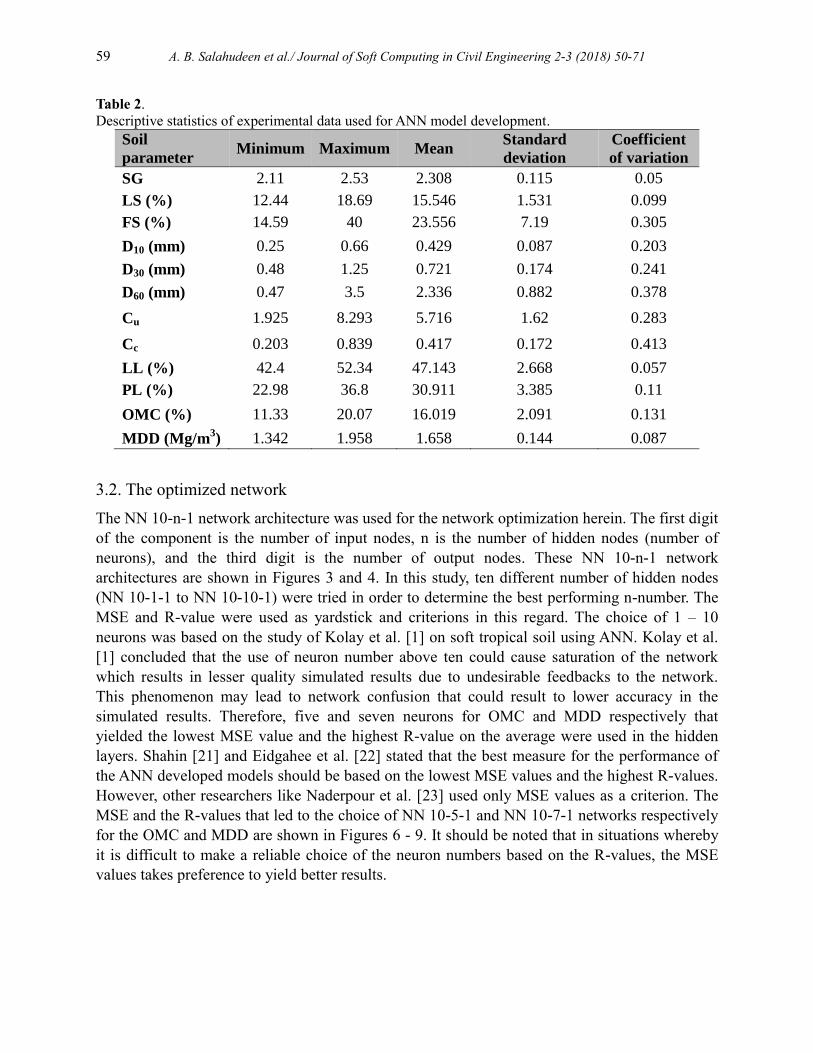
In ANN prediction modeling, the efficiency of input data and their ability to accurately predict
the output (target) is largely dependent on the relationship between the input and the output [19-
20]. In this study, ten input geotechnical soil parameters that have direct effects on the two
outputs were considered. The descriptive statistics of the experimental data as obtained from
various laboratory tests used for the ANN model development are presented in Table 2. In order
to give a detailed insight of the general data used for the study, a frequency bar chart was used to
present the research data of a total of 90 set as shown in Figures 5(a) – (l).

57 A. B. Salahudeen et al./ Journal of Soft Computing in Civil Engineering 2-3 (2018) 50-71
Fig. 5(a): Frequency of SG used for ANN Fig. 5(b): Frequency of FS used for ANN
Fig. 5(c): Frequency of LS used for ANN Fig. 5(d): Frequency of D10 used for ANN
Fig. 5(e): Frequency of D30 used for ANN Fig. 5(f): Frequency of Cc used for ANN
18
33
15
18
6
0
5
10
15
20
25
30
35
2.2 2.3 2.4 2.5 2.6
FR
EQ
UE
NC
Y
SPECIFIC GRAVITY
3
36
24
12
3
12
0
5
10
15
20
25
30
35
40
15 20 25 30 35 40
FR
EQ
UE
NC
Y
FREE SWELL (%)
6
18
30 27
9
0
5
10
15
20
25
30
35
13 14.5 16 17.5 19
FR
EQ
UE
NC
Y
LINEAR SHRINKAGE (%)
6
31
37
13
3
0
5
10
15
20
25
30
35
40
0.3 0.4 0.5 0.6 0.7
FR
EQ
UE
NC
Y
D10 (mm)
0
10
20
30
40
50
0.5 0.7 0.9 1.1 1.3
FR
EQ
UE
NC
Y
D30 (mm)
28
35
18
9
0
5
10
15
20
25
30
35
40
0.3 0.5 0.7 0.9
FR
EQ
UE
NC
Y
Cc

A. B. Salahudeen et al./ Journal of Soft Computing in Civil Engineering 2-3 (2018) 50-71 58
Fig. 5(g): Frequency of D60 used for ANN Fig. 5(h): Frequency of LL used for ANN
Fig. 5(i): Frequency of Cu used for ANN Fig. 5(j): Frequency of PL used for ANN
Fig. 5(k): Frequency of OMC for ANN Fig. 5(l): Frequency of MDD for ANN
1
12 10
2
12
40
0
5
10
15
20
25
30
35
40
45
0.5 1 1.5 2 2.5 3
FR
EQ
UE
NC
Y
D60 (mm)
6
18
24
21
12
9
0
5
10
15
20
25
43 45 47 49 51 53
FR
EQ
UE
NC
Y
LIQUID LIMIT (%)
2
16 16
55
1
0
10
20
30
40
50
60
2 4 6 8 10
FR
EQ
UE
NC
Y
Cu
3
6
15
27
30
9
0
5
10
15
20
25
30
35
23 26 29 32 35 38
FR
EQ
UE
NC
Y
PLASTIC LIMIT (%)
3
13
28 29
16
1
0
5
10
15
20
25
30
35
12 14 16 18 20 22
FR
EQ
UE
NC
Y
OPTIMUM MOISTURE CONTENT (%)
12
17
24 23
11
3
0
5
10
15
20
25
30
1.5 1.6 1.7 1.8 1.9 2
FR
EQ
UE
NC
Y
MAXIMUM DRY DENSITY (Mg/m3)
59 A. B. Salahudeen et al./ Journal of Soft Computing in Civil Engineering 2-3 (2018) 50-71
Table 2.
Descriptive statistics of experimental data used for ANN model development.
Soil
parameter Minimum Maximum Mean
Standard
deviation
Coefficient
of variation
SG 2.11 2.53 2.308 0.115 0.05
LS (%) 12.44 18.69 15.546 1.531 0.099
FS (%) 14.59 40 23.556 7.19 0.305
D10 (mm) 0.25 0.66 0.429 0.087 0.203
D30 (mm) 0.48 1.25 0.721 0.174 0.241
D60 (mm) 0.47 3.5 2.336 0.882 0.378
Cu 1.925 8.293 5.716 1.62 0.283
Cc 0.203 0.839 0.417 0.172 0.413
LL (%) 42.4 52.34 47.143 2.668 0.057
PL (%) 22.98 36.8 30.911 3.385 0.11
OMC (%) 11.33 20.07 16.019 2.091 0.131
MDD (Mg/m3) 1.342 1.958 1.658 0.144 0.087
3.2. The optimized network
The NN 10-n-1 network architecture was used for the network optimization herein. The first digit
of the component is the number of input nodes, n is the number of hidden nodes (number of
neurons), and the third digit is the number of output nodes. These NN 10-n-1 network
architectures are shown in Figures 3 and 4. In this study, ten different number of hidden nodes
(NN 10-1-1 to NN 10-10-1) were tried in order to determine the best performing n-number. The
MSE and R-value were used as yardstick and criterions in this regard. The choice of 1 – 10
neurons was based on the study of Kolay et al. [1] on soft tropical soil using ANN. Kolay et al.
[1] concluded that the use of neuron number above ten could cause saturation of the network
which results in lesser quality simulated results due to undesirable feedbacks to the network.
This phenomenon may lead to network confusion that could result to lower accuracy in the
simulated results. Therefore, five and seven neurons for OMC and MDD respectively that
yielded the lowest MSE value and the highest R-value on the average were used in the hidden
layers. Shahin [21] and Eidgahee et al. [22] stated that the best measure for the performance of
the ANN developed models should be based on the lowest MSE values and the highest R-values.
However, other researchers like Naderpour et al. [23] used only MSE values as a criterion. The
MSE and the R-values that led to the choice of NN 10-5-1 and NN 10-7-1 networks respectively
for the OMC and MDD are shown in Figures 6 - 9. It should be noted that in situations whereby
it is difficult to make a reliable choice of the neuron numbers based on the R-values, the MSE
values takes preference to yield better results.

A. B. Salahudeen et al./ Journal of Soft Computing in Civil Engineering 2-3 (2018) 50-71 60
Fig. 6. Variation of MSE with number of hidden layer neurons for OMC.
Fig. 7. Variation of MSE with number of hidden layer neurons for MDD.

61 A. B. Salahudeen et al./ Journal of Soft Computing in Civil Engineering 2-3 (2018) 50-71
Fig. 8. R-values for ANN performance with number of hidden layer neurons for OMC.
Fig. 9. R-values for ANN performance with number of hidden layer neurons for MDD.

A. B. Salahudeen et al./ Journal of Soft Computing in Civil Engineering 2-3 (2018) 50-71 62
3.3. ANN model development
The regression values for model performance evaluation showing the k (slope), R-values, MAE,
MSE and the RMSE are presented in Table 3. It is obvious from these statistical results that the
models developed in this study performed satisfactorily having high R-values and low error
values. The statistical parameters give acceptable results that make the confirmed the best
generalization of the developed model.
The variation of experimental and ANN predicted OMC and MDD values are shown in Figures
10 and 11 respectively. The performance of the simulated network was very good having k
values of 0.9654 for the OMC and 0.9364 for the MDD, where k is the slope of the regression
line through the origin in the plot of the experimental values to the predicted values. It was
reported by Alavi et al. [24] and Golbraikh and Tropsha [25] that the value of k should be close
to unity as a criterion for excellent performance.
Table 3.
Parameters and regression values for model performance evaluations.
Parameters OMC MDD
Number of Neurons 5 7
k 0.9654 0.9364
MSE (ANN) 0.0009 0.0022
R-Training 0.9977 0.9946
R-Testing 0.8855 0.9754
R-Validation 0.9779 0.9715
R-All Data 0.983 0.9884
MAE 0.0208 0.0229
MSE (Statistical) 0.0013 0.0010
RMSE 0.0358 0.0321
Fig. 10. Variation of experimental and ANN predicted OMC values.

63 A. B. Salahudeen et al./ Journal of Soft Computing in Civil Engineering 2-3 (2018) 50-71
Fig. 11. Variation of experimental and ANN predicted MDD values.
After the most acceptable and desirable network was chosen based on the highest R-value and
minimum MSE values and NN 10-5-1 and NN10-7-1 were selected as the best networks for
OMC and MDD respectively, the ANN was trained, and the training results are presented in
Figures 12 – 17 for the two targets. Figures 12 and 13 show the MSE of the network starting with
a higher value and decreasing to a smaller value. This shows that the network is learning until an
optimal target is achieved when the MSE is at its minimum. The three curves in these Figures
represent the three sets of data (training, testing, and validation) into which the total input and
output data were divided. The training of the neurons continues until the error reduced to its
minimum at which the network memorizes the training set then the training process is stopped.
This technique automatically avoids the problem of over-fitting, which plagues many
optimizations and learning algorithms.
The performance of the network based on its R-values for the three data sets are shown in
Figures 14 and 15 for the OMC and MDD respectively while the training state values showing
the gradient, input matrix of means (Mu) and the validation checking are shown in Figures 16
and 17 for OMC and MDD respectively.

A. B. Salahudeen et al./ Journal of Soft Computing in Civil Engineering 2-3 (2018) 50-71 64
Fig. 12. Performance of NN 10-5-1 by mean squared error for OMC.
Fig. 13. Performance of NN 10-7-1 by mean squared error for MDD.
0 2 4 6 8 10 1210
-5
10-4
10-3
10-2
10-1
100
Best Validation Performance is 0.00091478 at epoch 7
Mea
n S
qu
ared
Err
or
(mse
)
13 Epochs
Train
Validation
Test
Best
0 1 2 3 4 5 6 7 8 9 10 11
10-8
10-6
10-4
10-2
Best Validation Performance is 0.0022173 at epoch 5
Me
an
Sq
ua
red
Err
or
(m
se
)
11 Epochs
Train
Validation
Test
Best

65 A. B. Salahudeen et al./ Journal of Soft Computing in Civil Engineering 2-3 (2018) 50-71
Fig. 14. Regression values of NN 10-5-1 for OMC.
0.2 0.4 0.6 0.80.1
0.2
0.3
0.4
0.5
0.6
0.7
0.8
Target
Ou
tpu
t ~
= 0
.98
*Ta
rge
t +
0.0
08
7Training: R=0.99766
Data
Fit
Y = T
0.2 0.4 0.6 0.8
0.2
0.3
0.4
0.5
0.6
0.7
0.8
TargetO
utp
ut
~=
0.9
6*T
arg
et
+ 0
.02
9
Validation: R=0.9779
Data
Fit
Y = T
0.2 0.4 0.6 0.8
0.2
0.3
0.4
0.5
0.6
0.7
0.8
Target
Ou
tpu
t ~
= 0
.82
*Ta
rge
t +
0.0
77
Test: R=0.88553
Data
Fit
Y = T
0.2 0.4 0.6 0.80.1
0.2
0.3
0.4
0.5
0.6
0.7
0.8
Target
Ou
tpu
t ~
= 0
.97
*Ta
rge
t +
0.0
17
All: R=0.98298
Data
Fit
Y = T

A. B. Salahudeen et al./ Journal of Soft Computing in Civil Engineering 2-3 (2018) 50-71 66
Fig. 15. Regression values of NN 10-7-1 for MDD.
0.2 0.4 0.6 0.80.1
0.2
0.3
0.4
0.5
0.6
0.7
0.8
0.9
Target
Ou
tpu
t ~
= 0
.98
*Ta
rge
t +
0.0
14
Training: R=0.99462
Data
Fit
Y = T
0.2 0.4 0.6 0.8
0.2
0.3
0.4
0.5
0.6
0.7
0.8
0.9
Target
Ou
tpu
t ~
= 0
.97
*Ta
rge
t +
0.0
23
Validation: R=0.97146
Data
Fit
Y = T
0.2 0.4 0.6 0.8
0.2
0.3
0.4
0.5
0.6
0.7
0.8
0.9
Target
Ou
tpu
t ~
= 0
.98
*Ta
rge
t +
0.0
00
83
Test: R=0.97535
Data
Fit
Y = T
0.2 0.4 0.6 0.80.1
0.2
0.3
0.4
0.5
0.6
0.7
0.8
0.9
Target
Ou
tpu
t ~
= 0
.98
*Ta
rge
t +
0.0
11
All: R=0.98835
Data
Fit
Y = T

67 A. B. Salahudeen et al./ Journal of Soft Computing in Civil Engineering 2-3 (2018) 50-71
Fig. 16. Training state of NN 10-5-1 for OMC.
Fig. 17. Training state of NN 10-7-1 for MDD.
10-4
10-2
100
grad
ient
Gradient = 0.00068323, at epoch 13
10-5
10-4
10-3
mu
Mu = 1e-05, at epoch 13
0 2 4 6 8 10 120
5
10
val f
ail
13 Epochs
Validation Checks = 6, at epoch 13
10-5
100
grad
ient
Gradient = 6.5025e-05, at epoch 11
10-10
10-5
100
mu
Mu = 1e-08, at epoch 11
0 1 2 3 4 5 6 7 8 9 10 110
5
10
val f
ail
11 Epochs
Validation Checks = 6, at epoch 11

A. B. Salahudeen et al./ Journal of Soft Computing in Civil Engineering 2-3 (2018) 50-71 68
3.4. Model validation
The coefficient of correlation (R) is a measure used to evaluate the relative correlation and the
goodness-of-fit between the predicted and the observed data. Smith [26] suggested that a strong
correlation exists between any two sets of variables if the R-value is greater than 0.8. However,
Das and Sivakugan [27] are of the opinion that the use of R-value alone can be misleading
arguing that higher values of R may not necessarily indicate better model performance due to the
tendency of the model to deviate towards higher or lower values in a wide range data set.
The RMSE, on the other hand, is another measure of error in which large errors are given greater
concern than smaller errors. However, Shahin [21] argued that in contrast to the RMSE, MAE
eliminates the emphasis given to larger errors and that both RMSE and MAE are desirable when
the evaluated output data are continuous. Consequently, the combined use of R, RMSE and MAE
was found to yield a sufficient assessment of ANN model performance and allows comparison of
the accuracy of generalization of the predicted ANN model performance. This combination is
also sufficient to reveal any significant differences among the predicted and experimental data
sets.
Table 4.
Conditions of model validity.
Target Statistical
parameter Condition
Obtained
value Remarks
OMC
R > 0.8 0.983 Satisfactory
k Should be close to 1 0.9654 Satisfactory
MAE Should be close to 0 0.0208 Good
MSE Should be close to 0 0.0013 Satisfactory
RMSE Should be close to 0 0.0358 Good
MDD
R > 0.8 0.9884 Satisfactory
k Should be close to 1 0.9364 Satisfactory
MAE Should be close to 0 0.0229 Good
MSE Should be close to 0 0.001 Satisfactory
RMSE Should be close to 0 0.0321 Good
The conditions of model validity in this study are stated in Table 4. Based on the results of
different NN 10-n-1 networks used in this study, it was observed that the errors are at their best
performance when they are greater than 0.01 but still yield good and acceptable performance
when greater than 0.1 in a value range of 0 to 1. Based on the suggestion of Smith [26], the
argument of Das and Sivakugan [27], conclusions of Shahin [21] and observations in this study,
it is obvious from Table 4 that the developed model in this study performed satisfactorily and had
a good generalization potential. The achieved high R values and low values of errors are highly
desirable in ANN simulation as they indicate acceptable results. A strong correlation was
observed between the experimental OMC and MDD values as obtained by laboratory tests and
the predicted values using ANN. Ahmadi et al. [28], Naderpour et al. [29] and Eidgahee et al.
[22] reported that strong correlation exists between the experimental and predicted values if the
R-value is greater than 0.8, and the MSE values are at their minimum possible value. In a related

69 A. B. Salahudeen et al./ Journal of Soft Computing in Civil Engineering 2-3 (2018) 50-71
study by Naderpour et al. [23], R-values of 0.9346, 0.9686, 0.9442 and 0.944 were reported for
training, testing validation and their combination which were concluded to be satisfactory and
yielded good simulation results.
4. Conclusion
In this study, a soft computing approach, artificial neural networks (ANNs) was used to develop
an optimized predictive model for optimum moisture content (OMC) and maximum dry density
(MDD) of a cement kiln dust-stabilized black cotton soil. Based on the results of the developed
ANN model in this study, the following conclusions were made:
1. The multilayer perceptrons (MLPs) ANN used for the simulation of OMC and MDD of
CKD-stabilized black cotton soil that are trained with the feed forward back-propagation
algorithm performed satisfactorily.
2. The mean absolute error (MAE), root mean square error (RMSE) and R-value were used
as yardstick and criterions. In the neural network development, NN 10-5-1 and NN 10-7-
1 respectively for OMC and MDD that gave the lowest MSE value and the highest R-
value were used in the hidden layer of the architecture of the network and performed
satisfactorily.
3. For the normalized data used in training, testing and validating the neural network, the
performance of the simulated network was very good having R values of 0.983 and
0.9884 for the OMC and MDD respectively. These values met the minimum criteria of
0.8 conventionally recommended for strong correlation condition.
4. All the obtained simulation results are satisfactory, and a strong correlation was observed
between the experimental OMC and MDD values as obtained by laboratory tests and the
predicted values using ANN.
References
[1] Kolay P. K., Rosmina A. B., and Ling, N. W. (2008). “Settlement prediction of soft tropical soil by
Artificial Neural Network (ANN)”. The 12th International Conference of International Association
for Computer Methods and Advances in Geomechanics (IACMAG) pp.1843-1848.
[2] Shahin M. A., Jaksa M. B., Maier H. R. (2001). “Artificial neural network applications in
geotechnical engineering.” Australian Geomechanics, Vol. 36, No. 1, pp. 49-62.
[3] Maizir, H. and Kassim, K. A. (2013). “Neural network application in prediction of axial bearing
capacity of driven piles.” Proceedings of the International MultiConference of Engineers and
Computer Scientists Vol I.
[4] Eidgahee, D. R., Fasihi, F. and Naderpour, H. (2015). Optimized artificial neural network for amazing
soil-waste rubber shred mixture (in Persian). Sharif Journal of Civil Engineering, Vol. 31.2, No.
1.1, pp. 105 – 111.
[5] Fakharian, P., Naderpour, H., Haddad, A., Rafiean, A. H. and Eidgahee, D. R. (2018). A proposed
model for compressive strength prediction of FRP-confined rectangular column in terms of Genetic
expression Programming (GEP) (in Persian). Concrete Research.

A. B. Salahudeen et al./ Journal of Soft Computing in Civil Engineering 2-3 (2018) 50-71 70
[6] Shahin M.A., Maier H.R. and Jaksa M.B. (2002). “Predicting settlement of shallow foundations using
Neural Networks.” Journalof Geotechnical and Geoenvironmental Engineering, ASCE, Vol. 128
No. 9, pp. 785-793.
[7] Benali, A. Nechnech, A. and Ammar B. D. (2013). “Principal component analysis and Neural
Networks for predicting the pile capacity using SPT.” International Journal of Engineering and
Technology, Vol. 5, No. 1, February 2013.
[8] Van, D. B., Onyelowe, K. C., and Van-Nguyen, M. (2018). Capillary rise, suction (absorption) and the
strength development of HBM treated with QD base Geopolymer. International Journal of
Pavement Research and Technology.
[9] Phetchuay, C., Horpibulsuk, S., Arulrajah, A., Suksiripattanapong, C., and Udomchai, A. (2016).
Strength development in soft marine clay stabilized by fly ash and calcium carbide residue based
geopolymer. Applied Clay Science, Issue 127, pp. 134-142.
[10] Bui, V. D. and Onyolowe, K.C. (2018). Adsorbed complex and laboratory geotechnics of Quarry
Dust (QD) stabilized lateritic soils. Environmental Technology and Innovation., Issue 10, 3pp. 55-
363.
[11] Salahudeen, A. B., Eberemu O. A. and Osinubi, K. J. (2014). Assessment of cement kiln dust-treated
expansive soil for the construction of flexible pavements. Geotechnical and Geological
Engineering, Springer, Vol. 32, No. 4, PP. 923-931.
[12] Rahman M.K., Rehman S. and Al-Amoudi S.B. (2011). “Literature review on cement kiln dust usage
in soil and waste stabilization and experimental investigation” IJRRAS 7 pp. 77-78.
[13] Warren, K. W. and Kirby, T. M. (2004). “Expansive clay soil: A widespread and costly geohazard.”
Geostrata, Geo-Institute of the American Society Civil Engineers, Jan pp. 24-28.
[14] Balogun, L. A. (1991). “Effect of sand and salt additives on some geotechnical properties of lime
stabilized black cotton soil.” The Nigeria Engineer, Vol 26, No 2, pp. 15-24.
[15] Adeniji, F. A. (1991). “Recharge function of vertisolic Vadose zone in sub-sahelian Chad Basin.”
Proceedings 1st International Conference on Arid Zone Hydrology and Water Resource,
Maiduguri, pp. 331-348.
[16] Salahudeen, A. B. and Akiije, I. (2014). Stabilization of highway expansive soils with high loss on
ignition content kiln dust. Nigerian journal of technology (NIJOTECH), Vol. 33. No. 2, pp. 141 –
148.
[17] BS 1377 (1990). Methods of Testing Soil for Civil Engineering Purposes. British Standards
Institute, London.
[18] BS 1924 (1990). Methods of Tests for Stabilized Soils. British Standards Institute, London.
[19] Mikaeil, R., Shaffiee-Haghshenas, S., Ozcelik, Y., and Shaffiee-Haghshenas, S. (2017).
Development of Intelligent Systems to Predict Diamond Wire Saw Performance. Soft Computing in
Civil Engineering, Vol. 1, No. 2, pp. 52-69.
[20] Aryafar, A., Mikaeil, R., Doulati Ardejani, F., Shaffiee-Haghshenas, S., and Jafarpour, A. (2018).
Application of non-linear regression and soft computing techniques for modeling process of
pollutant adsorption from industrial wastewaters. Journal of Mining and Environment.
[21] Shahin, M. A. (2013). Artificial intelligence in geotechnical engineering: Applications, modelling
aspects and future directions. Metaheuristics in Water, Geotechnical and Transportation
Engineering, Elsevier, pp. 169 – 2014.
[22] Rezazadeh Eidgahee D, Haddad A, Naderpour H (2018) Evaluation of shear strength parameters of
granulated waste rubber using artificial neural networks and group method of data handling. Sci
Iran. https://doi.org/10.24200/sci.2018.5663.1408.
[23] Naderpour, H. Kheyroddin, A and Ghodrati-Amiri, G. (2010). “Prediction of FRP-confined
compressive strength of concrete using artificial neural networks.” Composite Structures, Issue 92,
pp. 2817–2829.

71 A. B. Salahudeen et al./ Journal of Soft Computing in Civil Engineering 2-3 (2018) 50-71
[24] Alavi, A. H., Ameri, M., Gandomi, A. H. and Mirzahosseini, M. R. (2011). Formulation of flow
number of asphalt mixes using a hybrid computational method, Construction Building Materials,
Vol. 25, No. 3, pp. 1338 – 1355.
[25] Golbraikh, A. and Tropsha, A. (2002). Beware of q2, J. Mol. Graph. Model., Vol. 20, No. 4, pp.
269–276.
[26] Smith, G. N. (1986). Probability and statistics in civil engineering. An Introduction, Collins, London.
[27] Das, S. K. and Sivakugan, N. (2010). Discussion of intelligent computing for modelling axial
capacity of pile foundations. Canadian Geotechnical Journal, Vol. 47, pp. 928 – 930.
[28] Ahmadi, M., Naderpour, H, and Kheyroddin, A. (2014). “Utilization of artificial neural networks to
prediction of the capacity of CCFT short columns subject to short term axial load.” Archives of civil
and mechanical engineering, issue 14, pp. 510 – 517.
[29] Naderpour, H., Rafiean, A.H. and Fakharian, P., (2018). Compressive strength prediction of
environmentally friendly concrete using artificial neural networks. Journal of Building
Engineering, Issue 16, pp. 213-219.