Embed Size (px)
Citation preview
Overview
1. Biological inspiration
2. Artificial neurons and neural networks
3. Learning processes
4. Learning with artificial neural networks
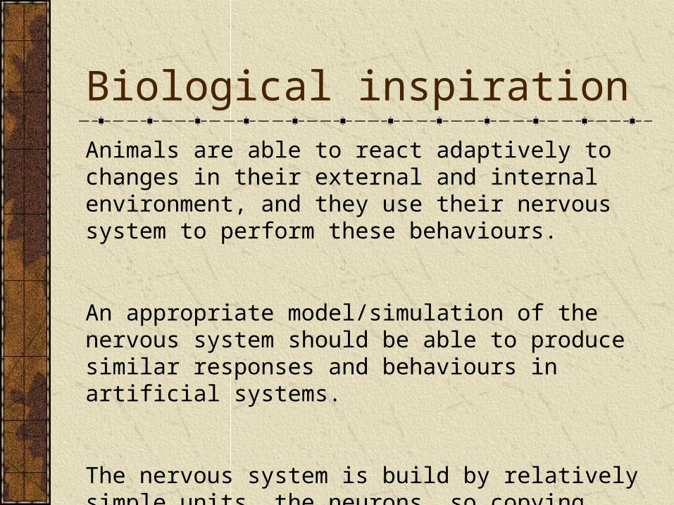
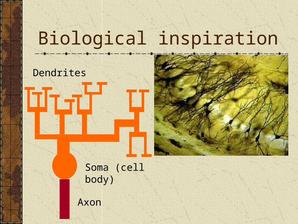
Biological inspiration
Animals are able to react adaptively to changes in their external and internal environment, and they use their nervous system to perform these behaviours.
An appropriate model/simulation of the nervous system should be able to produce similar responses and behaviours in artificial systems.
The nervous system is build by relatively simple units, the neurons, so copying their behavior and functionality should be the solution.
Biological inspiration
Dendrites
Soma (cell body)
Axon
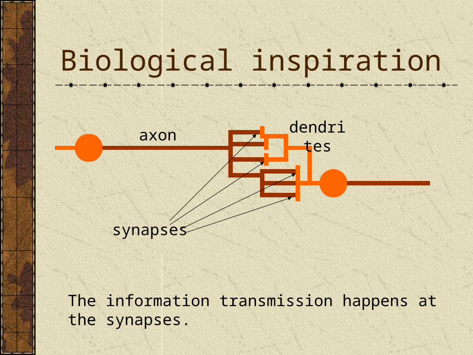
Biological inspiration
synapses
axon dendrites
The information transmission happens at the synapses.
Biological inspiration
The spikes travelling along the axon of the pre-synaptic neuron trigger the release of neurotransmitter substances at the synapse.
The neurotransmitters cause excitation or inhibition in the dendrite of the post-synaptic neuron.
The integration of the excitatory and inhibitory signals may produce spikes in the post-synaptic neuron.
The contribution of the signals depends on the strength of the synaptic connection.
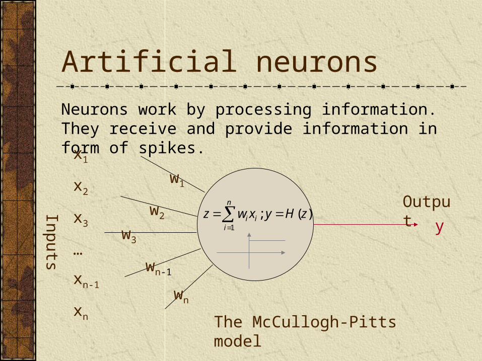
Artificial neurons
Neurons work by processing information. They receive and provide information in form of spikes.
The McCullogh-Pitts model
Inputs
Outputw2
w1
w3
wn
wn-1
. . .
x1
x2
x3
…
xn-1
xn
y)(;
1
zHyxwzn
iii
Artificial neurons
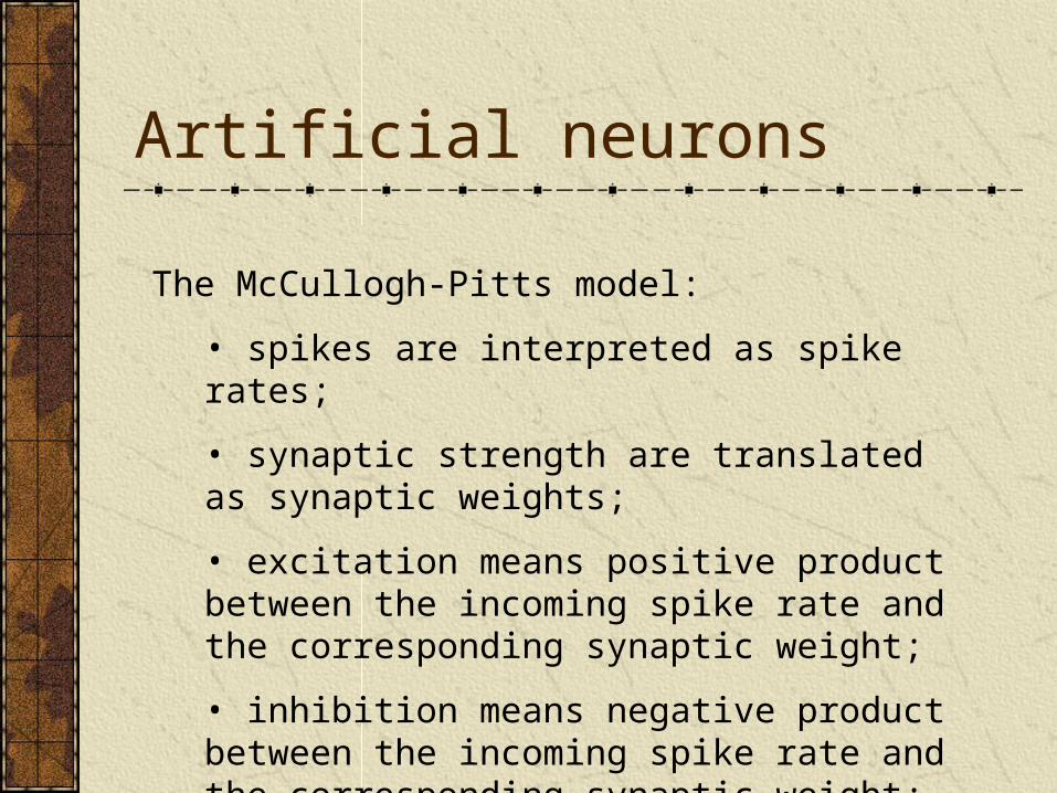
The McCullogh-Pitts model:
• spikes are interpreted as spike rates;
• synaptic strength are translated as synaptic weights;
• excitation means positive product between the incoming spike rate and the corresponding synaptic weight;
• inhibition means negative product between the incoming spike rate and the corresponding synaptic weight;
Artificial neurons
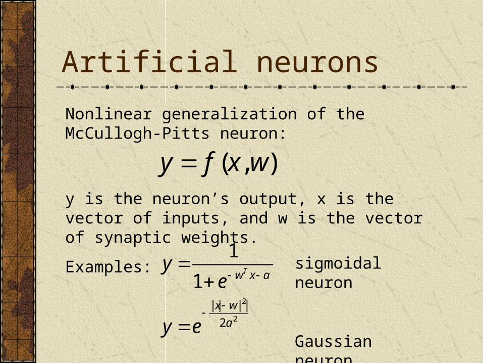
Nonlinear generalization of the McCullogh-Pitts neuron:
),( wxfy y is the neuron’s output, x is the vector of inputs, and w is the vector of synaptic weights.
Examples:
2
2
2
||||
1
1
a
wx
axw
ey
ey T
sigmoidal neuron
Gaussian neuron
Artificial neural networks
Inputs
Output
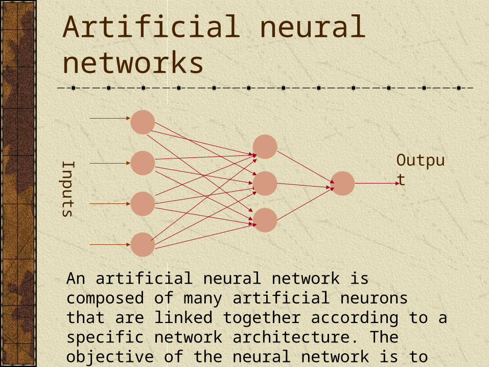
An artificial neural network is composed of many artificial neurons that are linked together according to a specific network architecture. The objective of the neural network is to transform the inputs into meaningful outputs.
Artificial neural networks
Tasks to be solved by artificial neural networks:
• controlling the movements of a robot based on self-perception and other information (e.g., visual information);
• deciding the category of potential food items (e.g., edible or non-edible) in an artificial world;
• recognizing a visual object (e.g., a familiar face);
• predicting where a moving object goes, when a robot wants to catch it.
Learning in biological systems
Learning = learning by adaptation
The young animal learns that the green fruits are sour, while the yellowish/reddish ones are sweet. The learning happens by adapting the fruit picking behavior.
At the neural level the learning happens by changing of the synaptic strengths, eliminating some synapses, and building new ones.
Learning as optimisation
The objective of adapting the responses on the basis of the information received from the environment is to achieve a better state. E.g., the animal likes to eat many energy rich, juicy fruits that make its stomach full, and makes it feel happy.
In other words, the objective of learning in biological organisms is to optimise the amount of available resources, happiness, or in general to achieve a closer to optimal state.
Learning in biological neural networks
The learning rules of Hebb:
• synchronous activation increases the synaptic strength;
• asynchronous activation decreases the synaptic strength.
These rules fit with energy minimization principles.
Maintaining synaptic strength needs energy, it should be maintained at those places where it is needed, and it shouldn’t be maintained at places where it’s not needed.
Learning principle for artificial neural networks
ENERGY MINIMIZATION
We need an appropriate definition of energy for artificial neural networks, and having that we can use mathematical optimisation techniques to find how to change the weights of the synaptic connections between neurons.
ENERGY = measure of task performance error
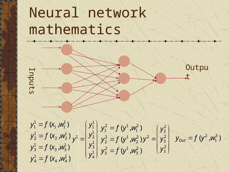
Neural network mathematics
Inputs
Output
),(
),(
),(
),(
144
14
133
13
122
12
111
11
wxfy
wxfy
wxfy
wxfy
),(
),(
),(
23
123
22
122
21
121
wyfy
wyfy
wyfy
14
13
12
11
1
y
y
y
y
y ),( 31
2 wyfyOut
23
23
23
2
y
y
y
y
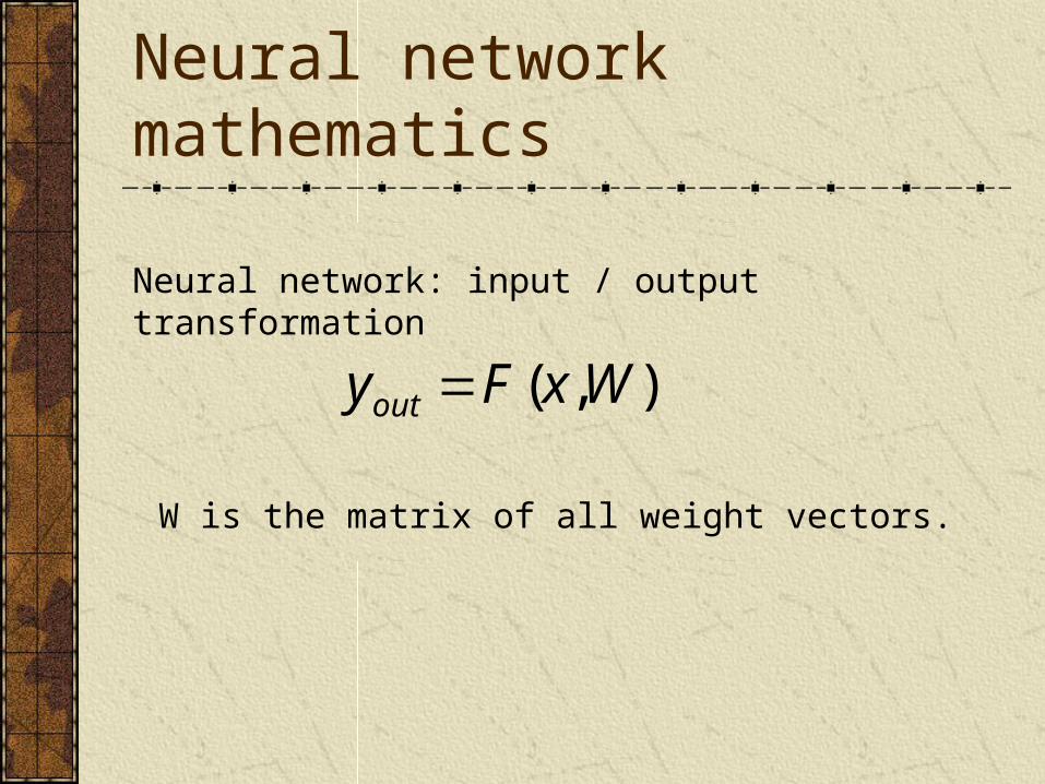
Neural network mathematics
Neural network: input / output transformation
),( WxFyout
W is the matrix of all weight vectors.
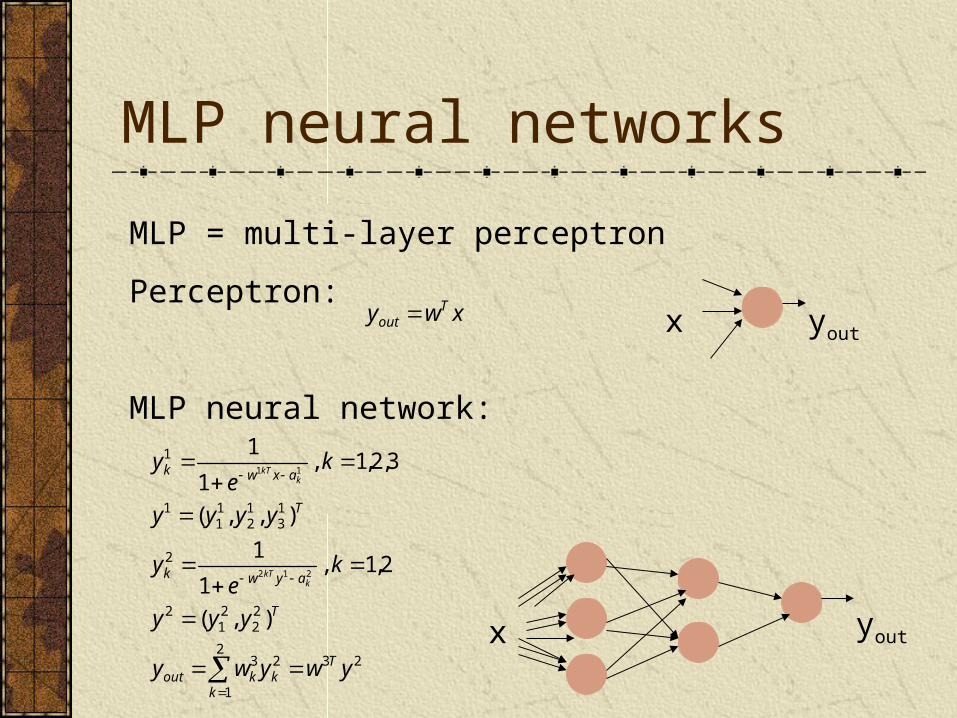
MLP neural networks
MLP = multi-layer perceptron
Perceptron:
MLP neural network:
xwy Tout x yout
x yout23
2
1
23
22
21
2
2
13
12
11
1
1
),(
2,1,1
1
),,(
3,2,1,1
1
212
11
ywywy
yyy
ke
y
yyyy
ke
y
T
kkkout
T
aywk
T
axwk
kkT
kkT
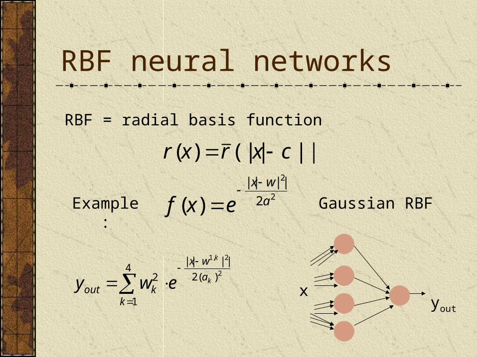
RBF neural networks
RBF = radial basis function
2
2
2
||||
)(
||)(||)(
a
wx
exf
cxrxr
Example: Gaussian RBF
xyout
4
1
)(2
||||
2 2
2,1
k
a
wx
koutk
k
ewy
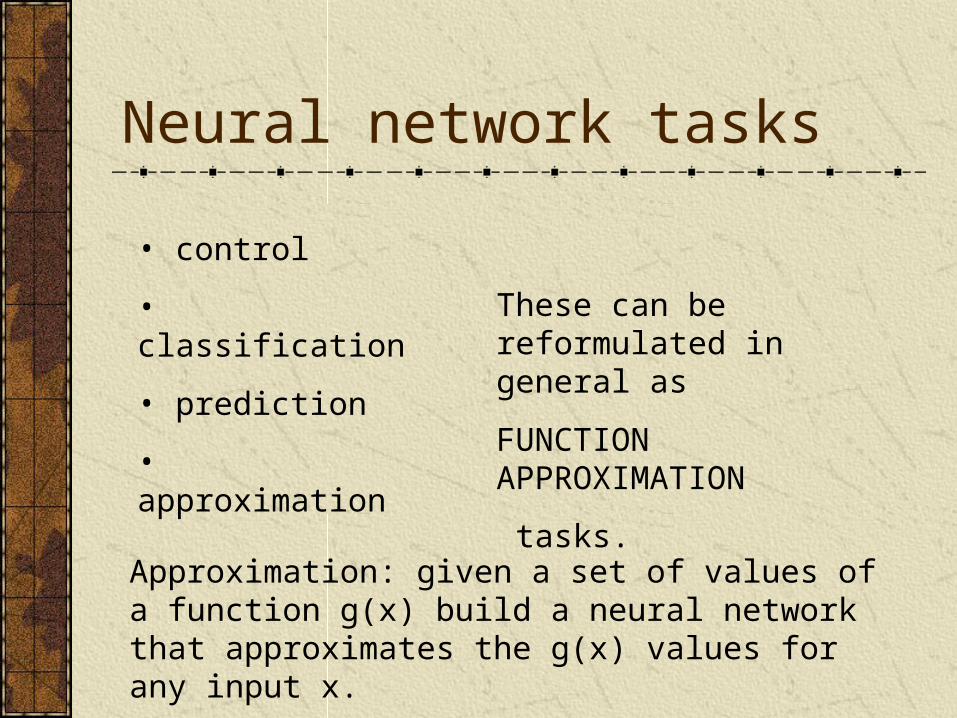
Neural network tasks
• control
• classification
• prediction
• approximation
These can be reformulated in general as
FUNCTION APPROXIMATION
tasks.
Approximation: given a set of values of a function g(x) build a neural network that approximates the g(x) values for any input x.
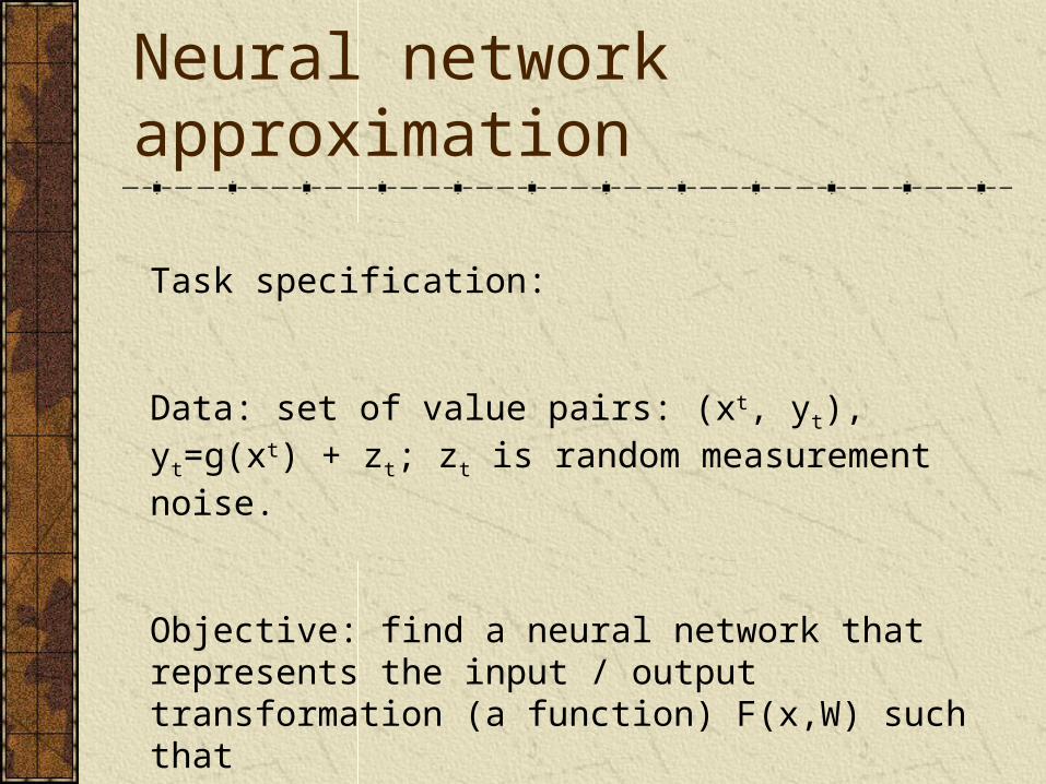
Neural network approximation
Task specification:
Data: set of value pairs: (xt, yt), yt=g(xt) + zt; zt is random measurement noise.
Objective: find a neural network that represents the input / output transformation (a function) F(x,W) such that
F(x,W) approximates g(x) for every x
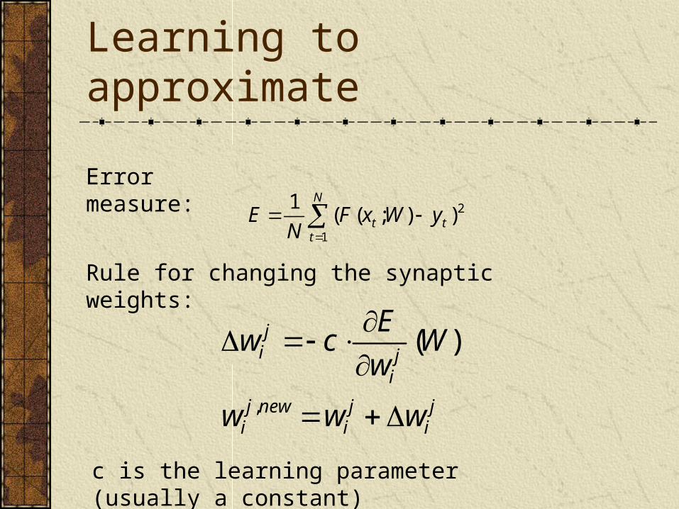
Learning to approximate
Error measure:
N
ttt yWxF
NE
1
2));((1
Rule for changing the synaptic weights:
ji
ji
newji
ji
ji
www
Ww
Ecw
,
)(
c is the learning parameter (usually a constant)
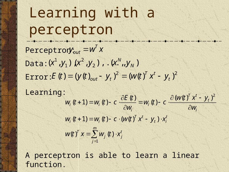
Learning with a perceptronPerceptron: xwy T
out
Data: ),(),...,,(),,( 22
11
NN yxyxyx
Error:22 ))(())(()( t
tTtout yxtwytytE
Learning:
tj
m
jj
T
tit
tTii
i
ttT
ii
ii
xtwxtw
xyxtwctwtw
w
yxtwctw
w
tEctwtw
1
2
)()(
))(()()1(
))(()(
)()()1(
A perceptron is able to learn a linear function.
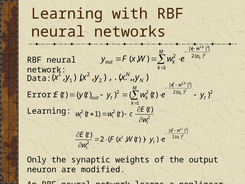
Learning with RBF neural networks
RBF neural network:
Data: ),(),...,,(),,( 22
11
NN yxyxyx
Error: 2
1
)(2
||||
22 ))(())(()(2
2,1
t
M
k
a
wx
ktout yetwytytE k
kt
Learning:
2
2,1
)(2
||||
2
222
)))(,((2)(
)()()1(
i
it
a
wx
tt
i
iii
eytWxFw
tE
w
tEctwtw
Only the synaptic weights of the output neuron are modified.
An RBF neural network learns a nonlinear function.
M
k
a
wx
koutk
k
ewWxFy1
)(2
||||
2 2
2,1
),(
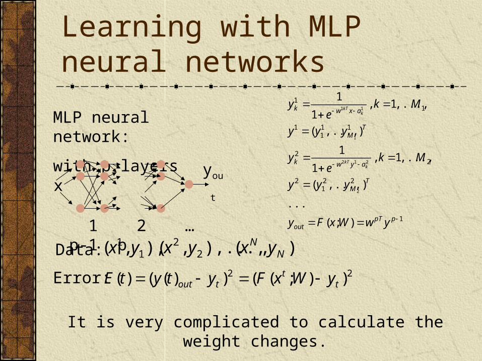
Learning with MLP neural networks
MLP neural network:
with p layers
Data: ),(),...,,(),,( 22
11
NN yxyxyx
Error: 22 ));(())(()( tt
tout yWxFytytE
1
221
2
22
111
1
11
);(
...
),...,(
,...,1,1
1
),...,(
,...,1,1
1
2
212
1
11
ppTout
TM
aywk
TM
axwk
ywWxFy
yyy
Mke
y
yyy
Mke
y
kkT
kkT
It is very complicated to calculate the weight changes.
xyout
1 2 … p-1 p
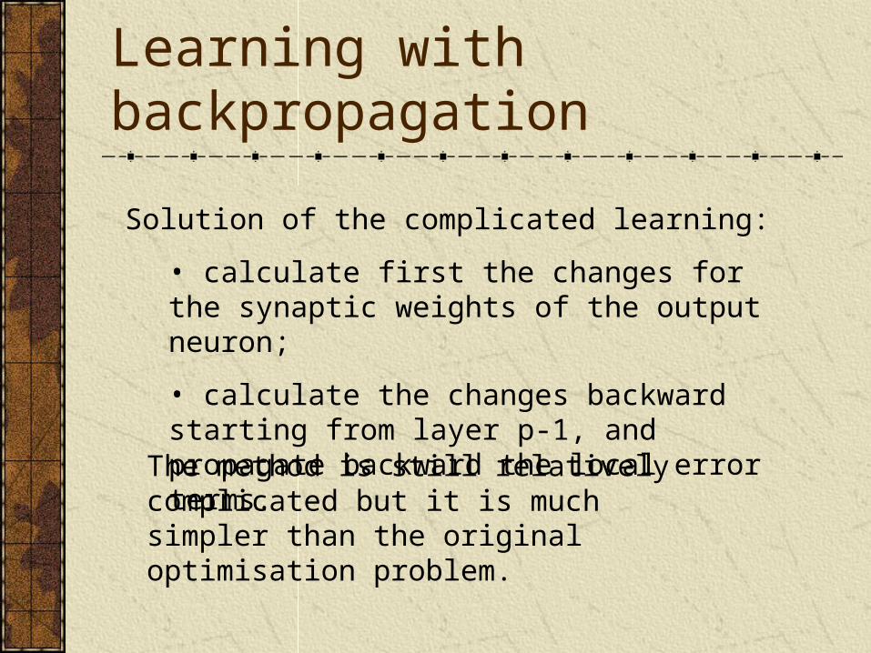
Learning with backpropagation
Solution of the complicated learning:
• calculate first the changes for the synaptic weights of the output neuron;
• calculate the changes backward starting from layer p-1, and propagate backward the local error terms.
The method is still relatively complicated but it is much simpler than the original optimisation problem.
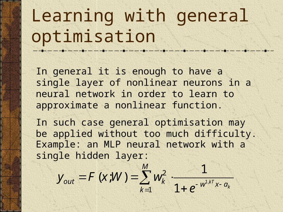
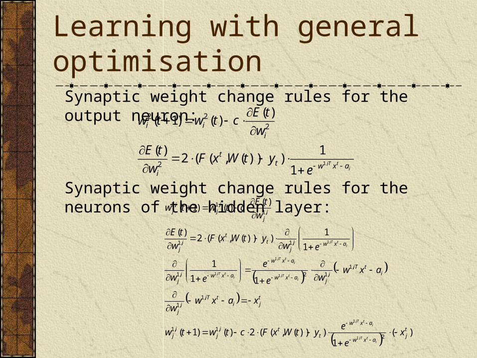
Learning with general optimisation
In general it is enough to have a single layer of nonlinear neurons in a neural network in order to learn to approximate a nonlinear function.
In such case general optimisation may be applied without too much difficulty.
Example: an MLP neural network with a single hidden layer:
M
kaxwkoutk
kT
ewWxFy
1
2,1
1
1);(
Learning with general optimisation
itiT axwt
t
i
iii
eytWxF
w
tE
w
tEctwtw
,1
1
1)))(,((2
)(
)()()1(
2
222
Synaptic weight change rules for the output neuron:
Synaptic weight change rules for the neurons of the hidden layer:
)(1
)))(,((2)()1(
11
1
1
1)))(,((2
)(
)()()1(
2,1,1
,1,1
,1,12,1
,1,1
,1,1,1
,1
,1
,1
,1
,1
,1
tj
axw
axw
tti
jij
tji
tiTij
itiT
ij
axw
axw
axwij
axwij
tt
ij
ij
ij
ij
xe
eytWxFctwtw
xaxww
axwwe
e
ew
ewytWxF
w
tE
w
tEctwtw
itiT
itiT
itiT
itiT
itiT
itiT
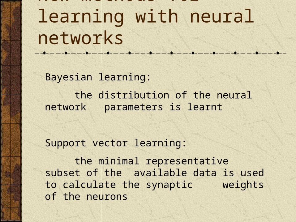
New methods for learning with neural networks
Bayesian learning:
the distribution of the neural network parameters is learnt
Support vector learning:
the minimal representative subset of the available data is used to calculate the synaptic weights of the neurons
Summary
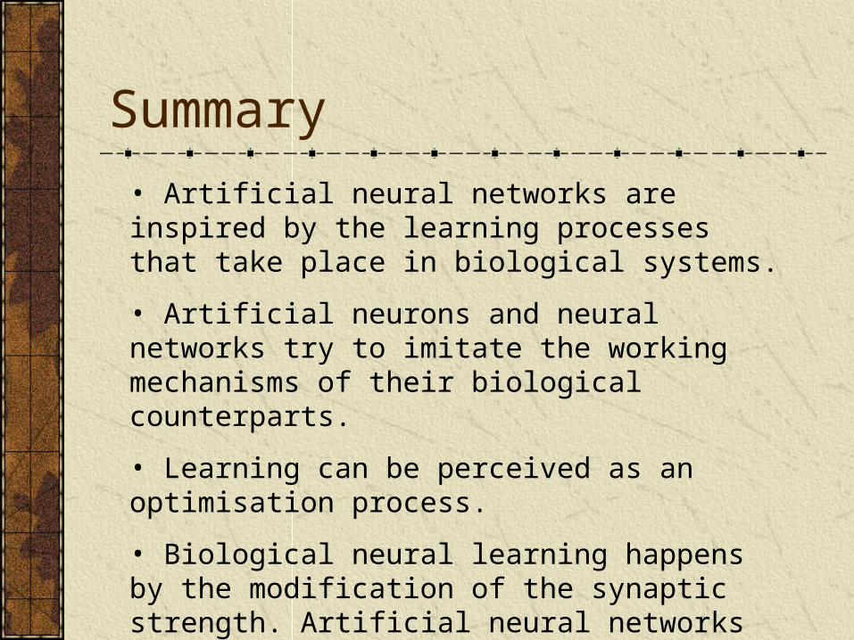
• Artificial neural networks are inspired by the learning processes that take place in biological systems.
• Artificial neurons and neural networks try to imitate the working mechanisms of their biological counterparts.
• Learning can be perceived as an optimisation process.
• Biological neural learning happens by the modification of the synaptic strength. Artificial neural networks learn in the same way.
• The synapse strength modification rules for artificial neural networks can be derived by applying mathematical optimisation methods.
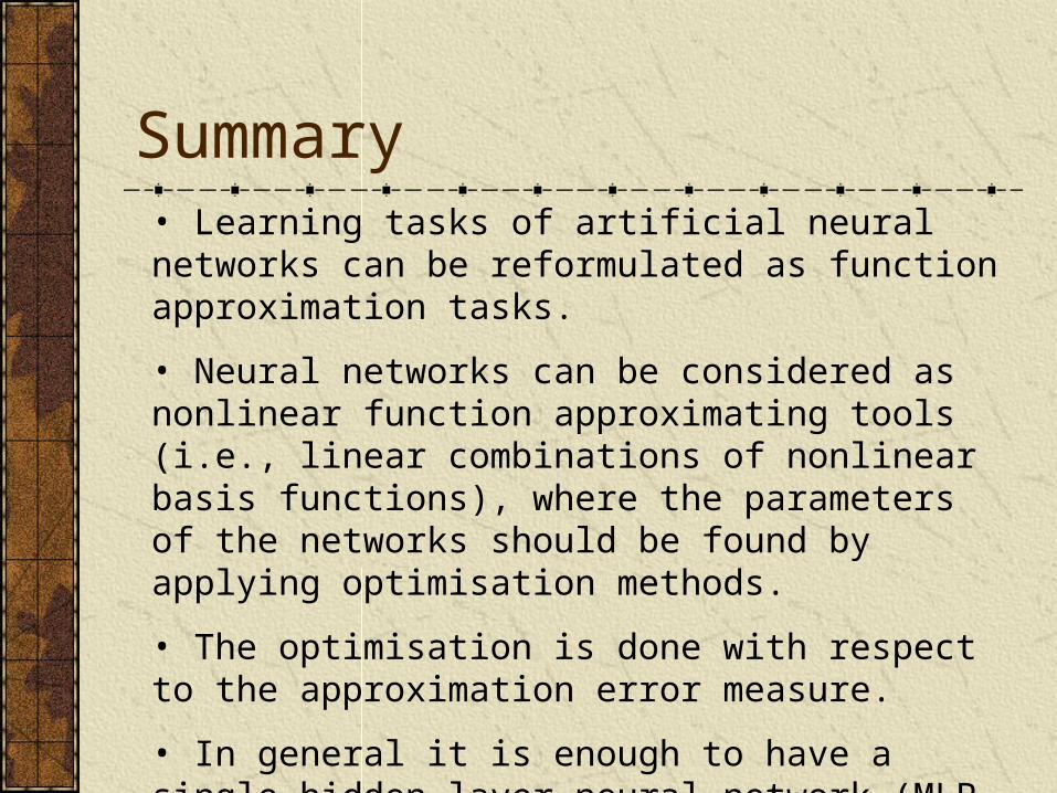
Summary• Learning tasks of artificial neural networks can be reformulated as function approximation tasks.
• Neural networks can be considered as nonlinear function approximating tools (i.e., linear combinations of nonlinear basis functions), where the parameters of the networks should be found by applying optimisation methods.
• The optimisation is done with respect to the approximation error measure.
• In general it is enough to have a single hidden layer neural network (MLP, RBF or other) to learn the approximation of a nonlinear function. In such cases general optimisation can be applied to find the change rules for the synaptic weights.