Embed Size (px)
Citation preview
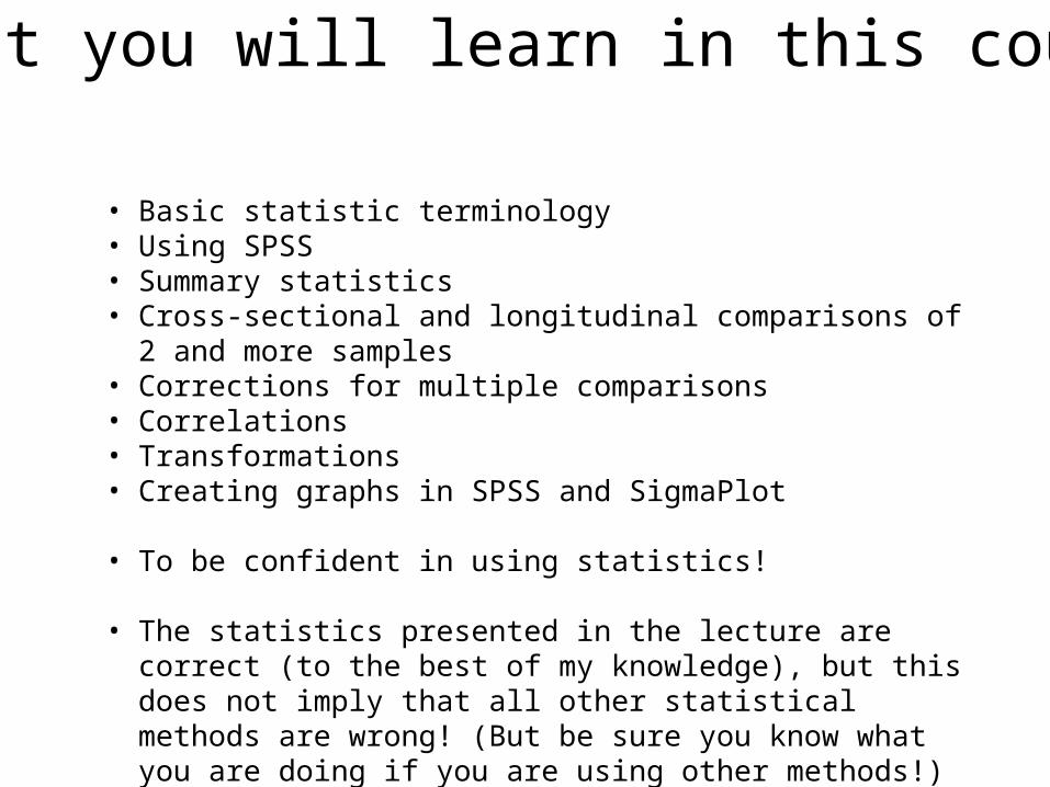
• Basic statistic terminology• Using SPSS• Summary statistics• Cross-sectional and longitudinal comparisons of 2 and more samples• Corrections for multiple comparisons• Correlations• Transformations• Creating graphs in SPSS and SigmaPlot
• To be confident in using statistics!
• The statistics presented in the lecture are correct (to the best of my knowledge), but this does not imply that all other statistical methods are wrong! (But be sure you know what you are doing if you are using other methods!)
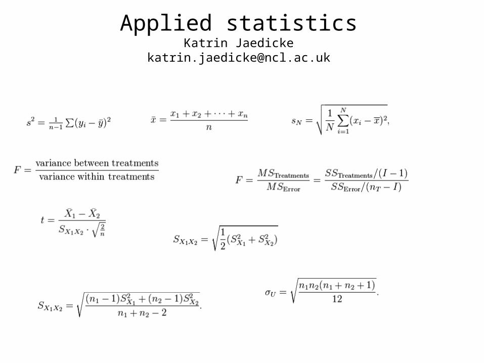
What you will learn in this course
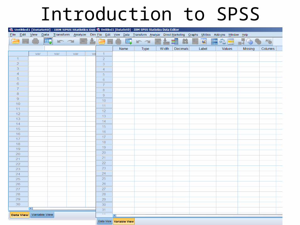
Introduction to SPSS
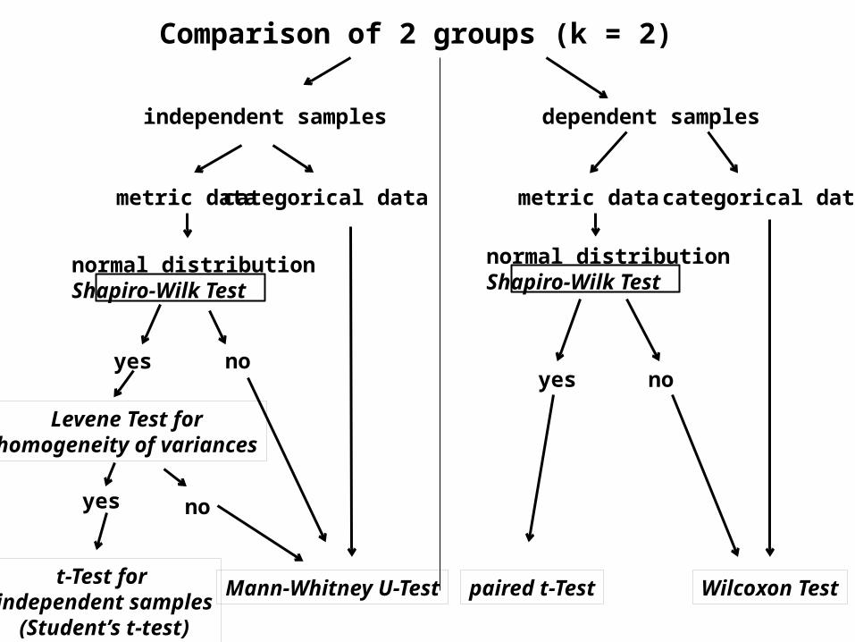
Comparison of 2 groups (k = 2)
independent samples dependent samples
metric data categorical data metric data categorical data
normal distributionShapiro-Wilk Test
yes no
t-Test for independent samples
(Student’s t-test)
Mann-Whitney U-Test paired t-Test Wilcoxon Test
normal distributionShapiro-Wilk Test
yes no
Levene Test forhomogeneity of variances
yes no
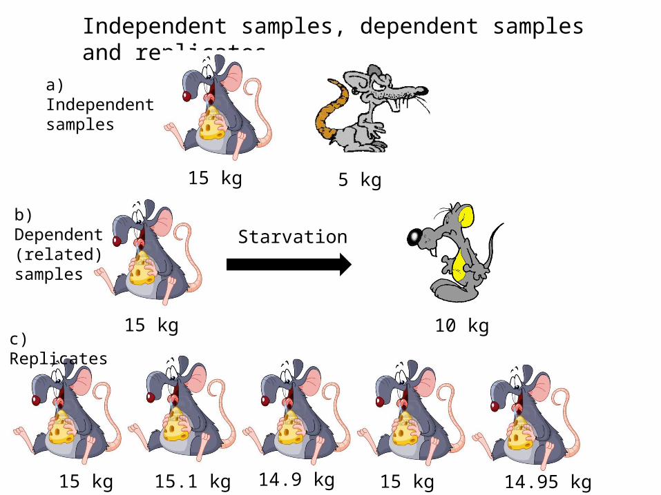
Independent samples, dependent samples and replicates
15 kg 5 kg
15 kg
Starvation
10 kg
15.1 kg15 kg 14.9 kg 15 kg 14.95 kg
a) Independent samples
b) Dependent (related) samples
c) Replicates
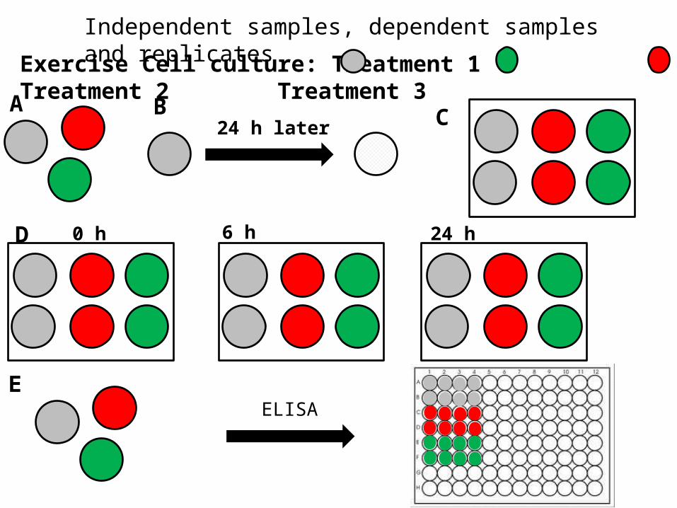
Exercise Cell culture: Treatment 1 Treatment 2 Treatment 3
A B24 h later
Independent samples, dependent samples and replicates
C
D 0 h 6 h 24 h
EELISA
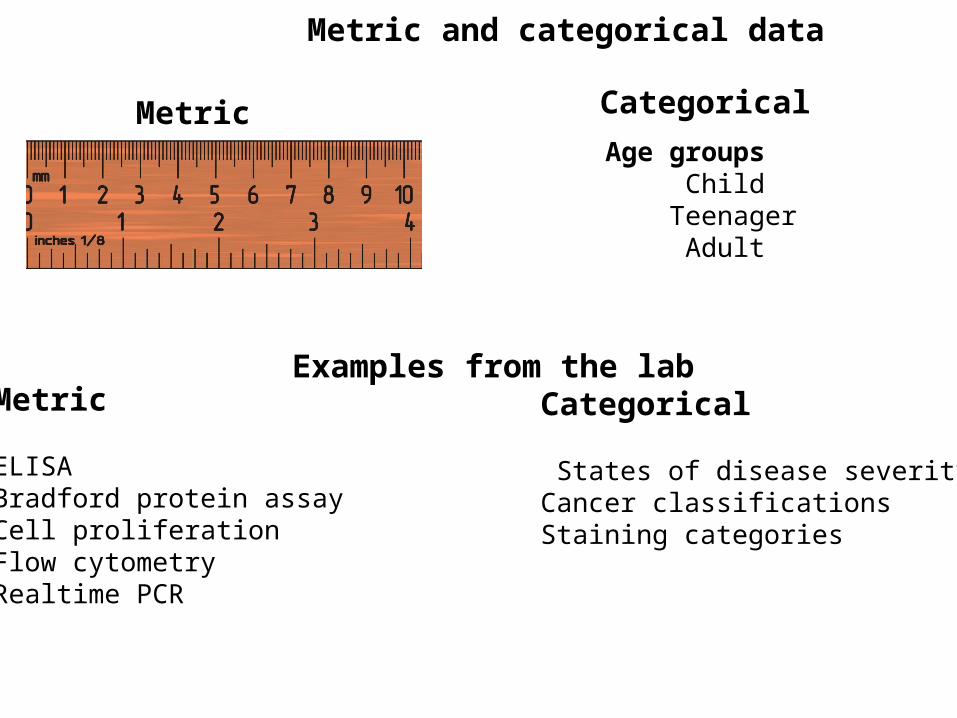
Metric and categorical data
Age groups Child Teenager Adult
Examples from the labMetric
ELISABradford protein assayCell proliferationFlow cytometryRealtime PCR
Categorical
States of disease severityCancer classificationsStaining categories
Metric Categorical
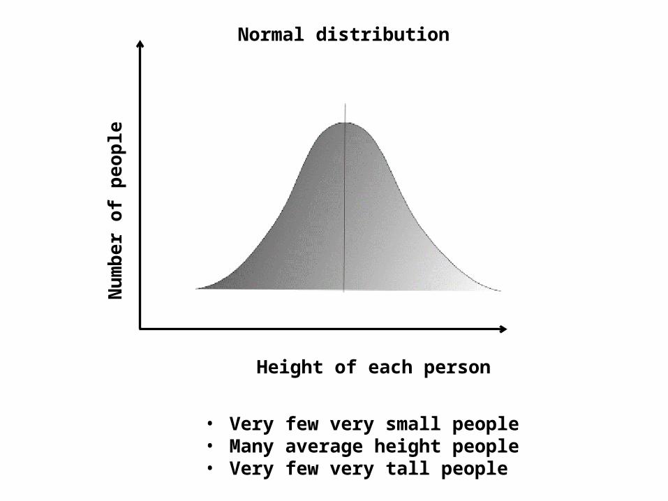
Normal distribution
Height of each person
Num
ber o
f peo
ple
• Very few very small people• Many average height people• Very few very tall people
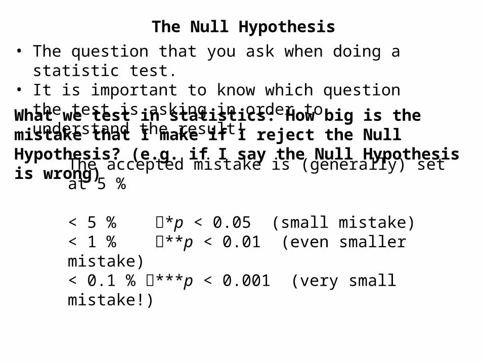
The Null Hypothesis• The question that you ask when doing a statistic test. • It is important to know which question the test is asking in
order to understand the result!
The accepted mistake is (generally) set at 5 %
< 5 % *p < 0.05 (small mistake)< 1 % **p < 0.01 (even smaller mistake)< 0.1 % ***p < 0.001 (very small mistake!)
What we test in statistics: How big is the mistake that I make if I reject the Null Hypothesis? (e.g. if I say the Null Hypothesis is wrong)
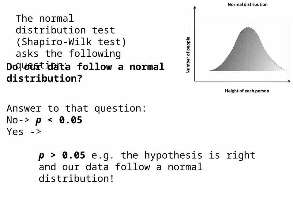
The normal distribution test (Shapiro-Wilk test) asks the following question:
p > 0.05 e.g. the hypothesis is right and our data follow a normal distribution!
Answer to that question:No-> p < 0.05Yes ->
Do our data follow a normal distribution?
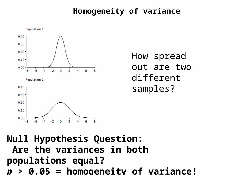
Homogeneity of variance
How spread out are two different samples?
Null Hypothesis Question: Are the variances in both populations equal?p > 0.05 = homogeneity of variance!
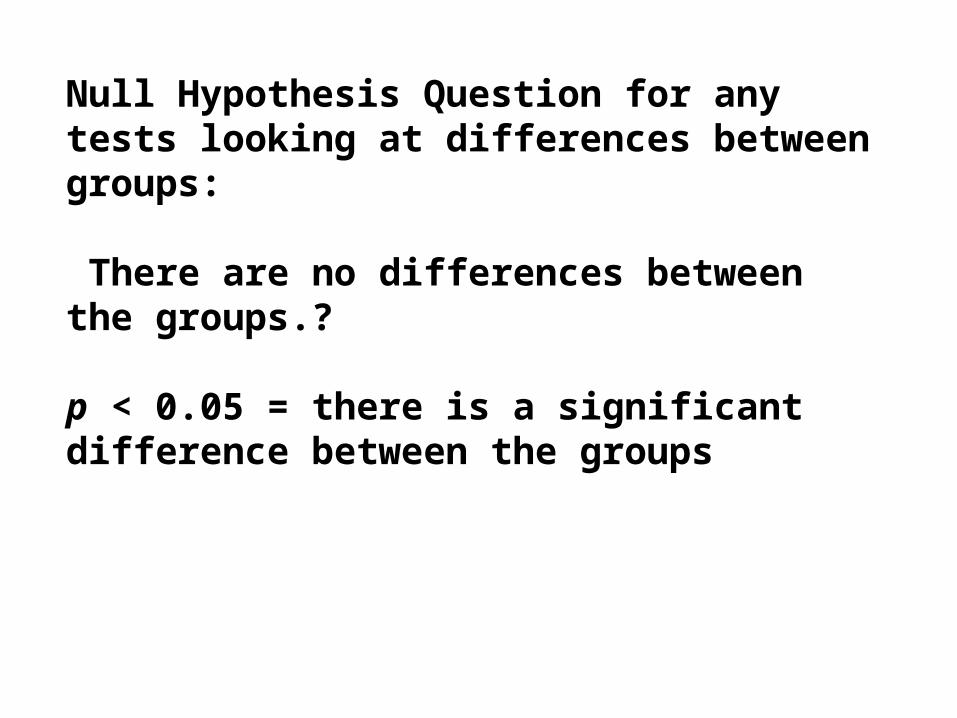
Null Hypothesis Question for any tests looking at differences between groups:
There are no differences between the groups.?
p < 0.05 = there is a significant difference between the groups
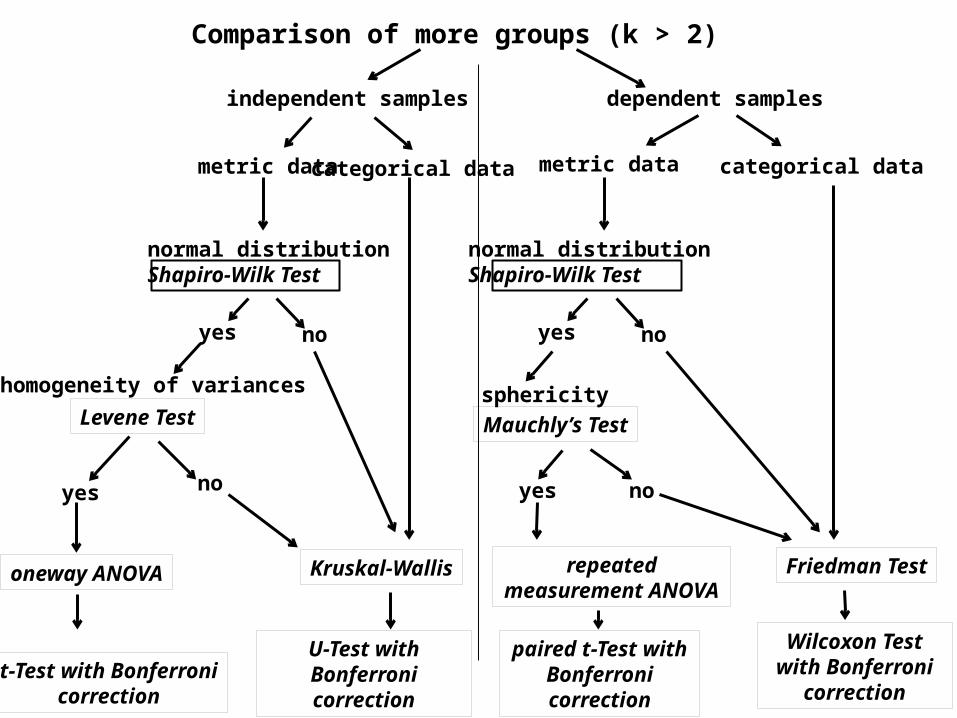
Comparison of more groups (k > 2)
independent samples dependent samples
metric data categorical data
normal distributionShapiro-Wilk Test
yes no
t-Test with Bonferronicorrection
U-Test with Bonferronicorrection
Levene Testhomogeneity of variances
yes no
oneway ANOVA Kruskal-Wallis
metric data categorical data
paired t-Test with Bonferroni correction
Wilcoxon Test with Bonferroni correction
repeated measurement ANOVA
Friedman Test
normal distributionShapiro-Wilk Test
yes no
Mauchly’s Testsphericity
yes no
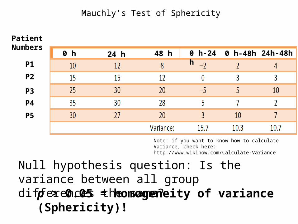
Mauchly’s Test of Sphericity
Null hypothesis question: Is the variance between all group differences the same?
p > 0.05 = homogeneity of variance (Sphericity)!
P1
P2
Patient Numbers
P3
P4
P5
0 h 24 h 48 h 0 h-24 h 0 h-48h 24h-48h
Note: if you want to know how to calculate Variance, check here: http://www.wikihow.com/Calculate-Variance
Ser
um
pro
tein
0
100
200
300
control A B C
******
*
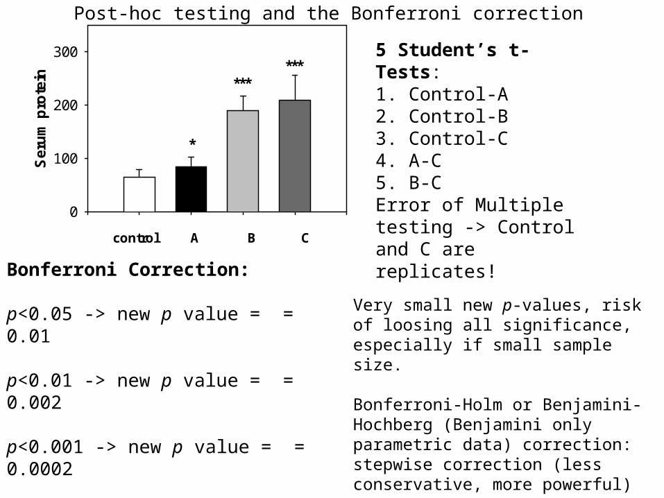
Post-hoc testing and the Bonferroni correction
5 Student’s t-Tests: 1. Control-A2. Control-B3. Control-C4. A-C5. B-CError of Multiple testing -> Control and C are replicates!
Bonferroni Correction:
p<0.05 -> new p value = = 0.01
p<0.01 -> new p value = = 0.002
p<0.001 -> new p value = = 0.0002
Very small new p-values, risk of loosing all significance, especially if small sample size.
Bonferroni-Holm or Benjamini-Hochberg (Benjamini only parametric data) correction: stepwise correction (less conservative, more powerful)
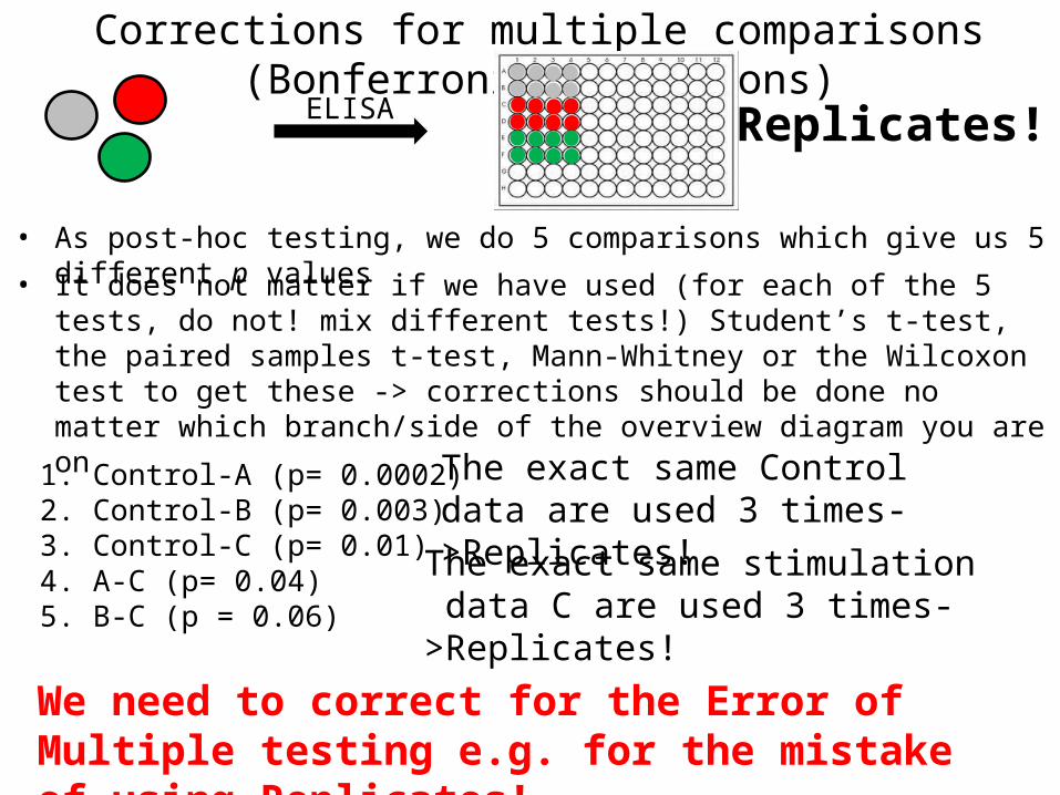
Corrections for multiple comparisons (Bonferroni corrections)
ELISA
1. Control-A (p= 0.0002)2. Control-B (p= 0.003)3. Control-C (p= 0.01)4. A-C (p= 0.04)5. B-C (p = 0.06)
Replicates!
• As post-hoc testing, we do 5 comparisons which give us 5 different p values
The exact same Control data are used 3 times->Replicates!
The exact same stimulation data C are used 3 times->Replicates!
We need to correct for the Error of Multiple testing e.g. for the mistake of using Replicates!
• It does not matter if we have used (for each of the 5 tests, do not! mix different tests!) Student’s t-test, the paired samples t-test, Mann-Whitney or the Wilcoxon test to get these -> corrections should be done no matter which branch/side of the overview diagram you are on
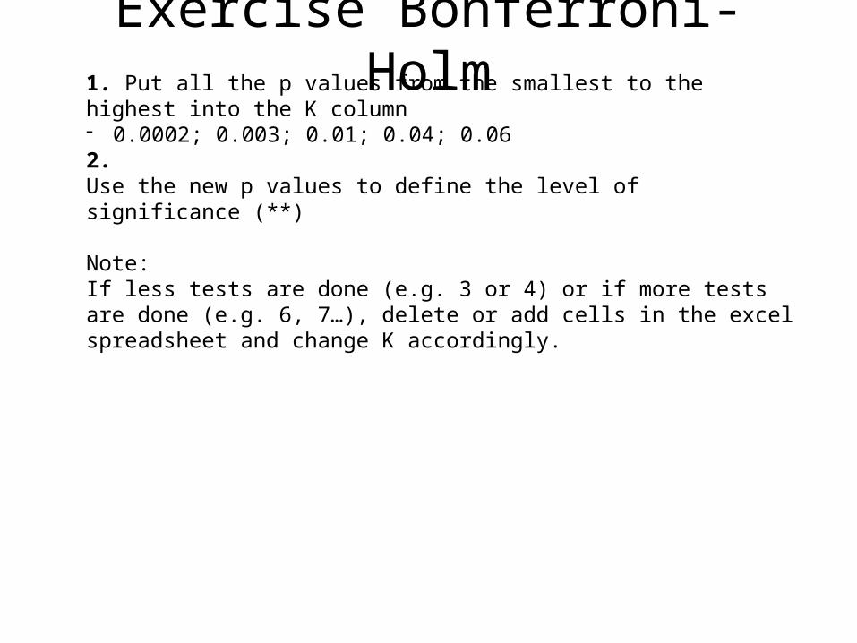
Exercise Bonferroni-Holm1. Put all the p values from the smallest to the highest into the K column- 0.0002; 0.003; 0.01; 0.04; 0.062. Use the new p values to define the level of significance (**)
Note:If less tests are done (e.g. 3 or 4) or if more tests are done (e.g. 6, 7…), delete or add cells in the excel spreadsheet and change K accordingly.
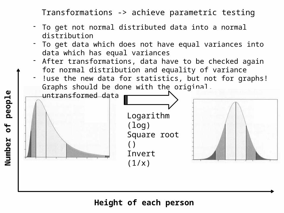
Transformations -> achieve parametric testing
Height of each person
Num
ber o
f peo
ple
- To get not normal distributed data into a normal distribution- To get data which does not have equal variances into data which has equal
variances- After transformations, data have to be checked again for normal distribution
and equality of variance- !use the new data for statistics, but not for graphs! Graphs should be done
with the original, untransformed data
Logarithm (log)Square root ()Invert (1/x)
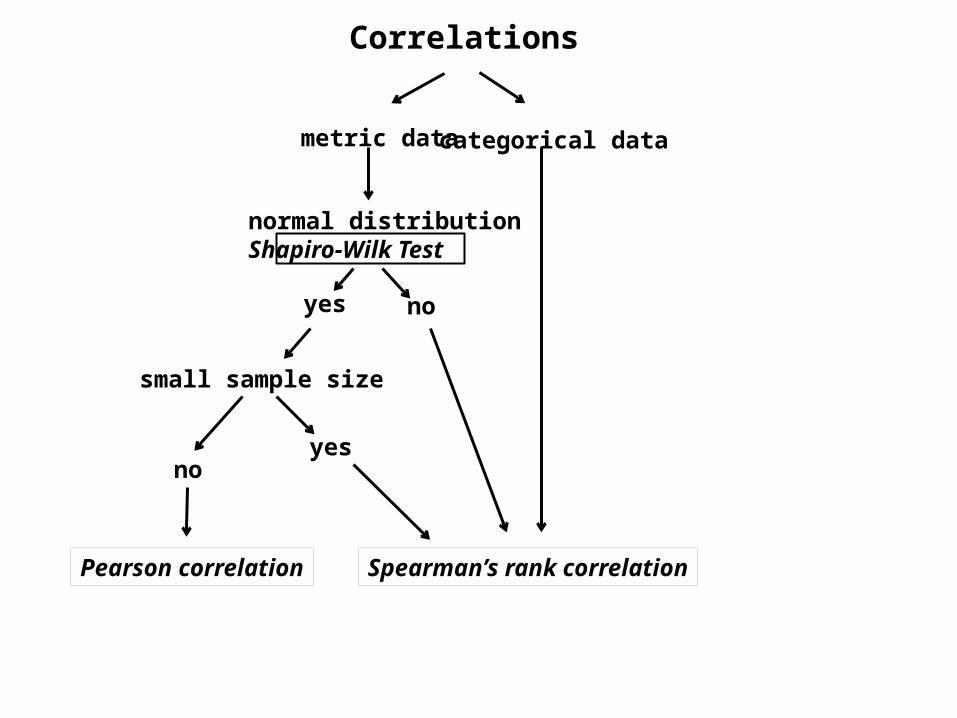
Correlations
metric data categorical data
normal distributionShapiro-Wilk Test
yes no
small sample size
yesno
Pearson correlation Spearman’s rank correlation
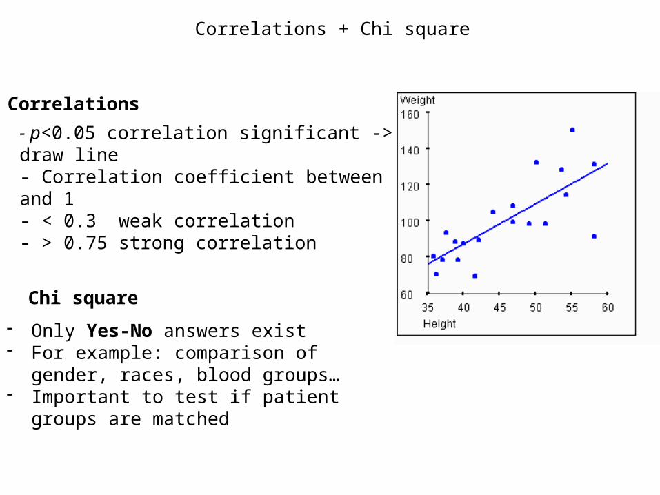
- p<0.05 correlation significant -> draw line- Correlation coefficient between 0 and 1 - < 0.3 weak correlation- > 0.75 strong correlation
Correlations + Chi square
Correlations
Chi square
- Only Yes-No answers exist- For example: comparison of gender, races,
blood groups… - Important to test if patient groups are matched
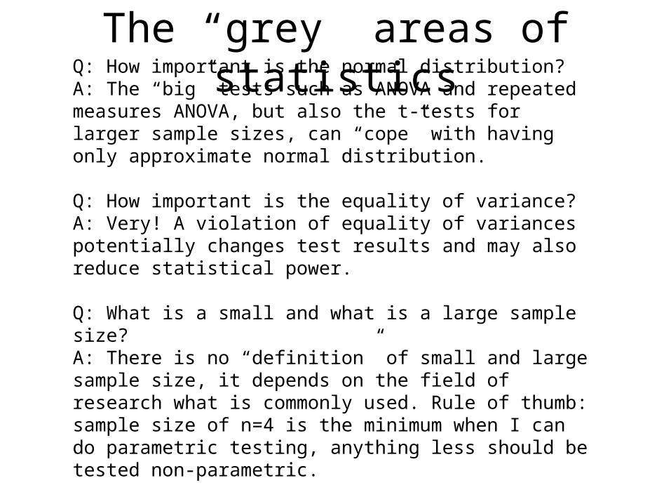
The “grey” areas of statisticsQ: How important is the normal distribution?A: The “big” tests such as ANOVA and repeated measures ANOVA, but also the t-tests for larger sample sizes, can “cope” with having only approximate normal distribution.
Q: How important is the equality of variance?A: Very! A violation of equality of variances potentially changes test results and may also reduce statistical power.
Q: What is a small and what is a large sample size?A: There is no “definition” of small and large sample size, it depends on the field of research what is commonly used. Rule of thumb: sample size of n=4 is the minimum when I can do parametric testing, anything less should be tested non-parametric.
Q: Do I always have to correct for multiple comparisons?A: No, but you have stronger results if your p-values are still significant after correction and they are less likely being open to criticism of being a “chance” finding.
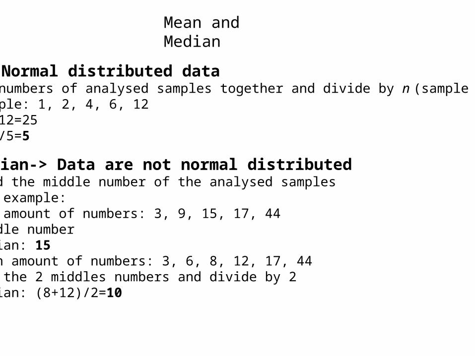
Mean and Median
Mean-> Normal distributed dataAdd all numbers of analysed samples together and divide by n (sample size)For example: 1, 2, 4, 6, 121+2+4+6+12=25Mean: 25/5=5
Median-> Data are not normal distributedFind the middle number of the analysed samples For example:Odd amount of numbers: 3, 9, 15, 17, 44 Middle numberMedian: 15Even amount of numbers: 3, 6, 8, 12, 17, 44Add the 2 middles numbers and divide by 2Median: (8+12)/2=10
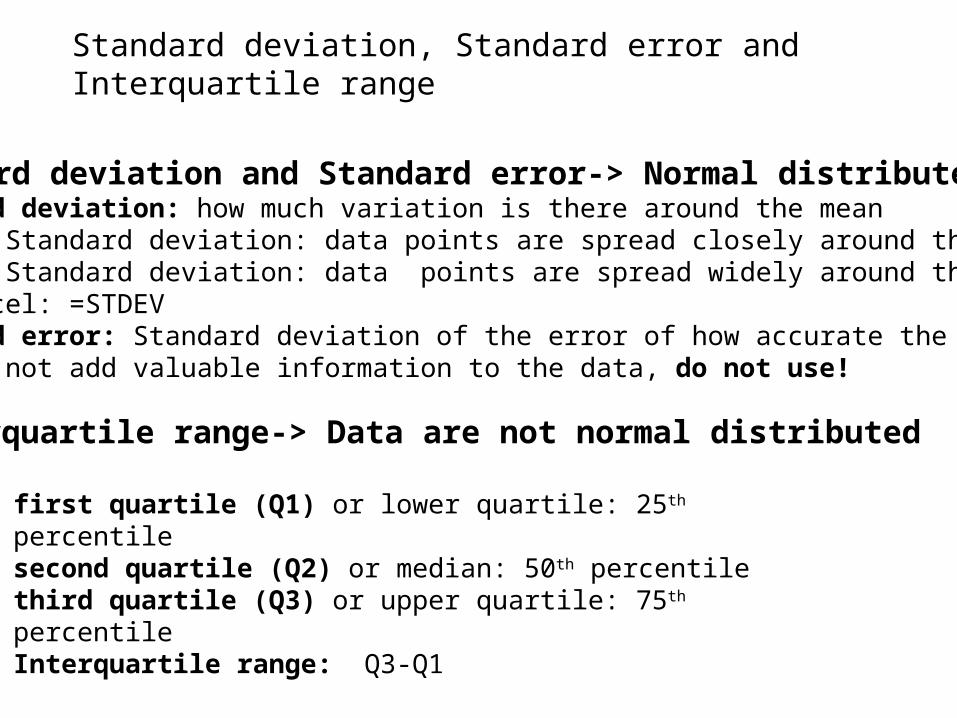
Standard deviation, Standard error and Interquartile range
Standard deviation and Standard error-> Normal distributed dataStandard deviation: how much variation is there around the mean- Small Standard deviation: data points are spread closely around the mean- Large Standard deviation: data points are spread widely around the mean- In Excel: =STDEVStandard error: Standard deviation of the error of how accurate the mean is-> does not add valuable information to the data, do not use!
Interquartile range-> Data are not normal distributed
first quartile (Q1) or lower quartile: 25th percentile second quartile (Q2) or median: 50th percentilethird quartile (Q3) or upper quartile: 75th percentileInterquartile range: Q3-Q1
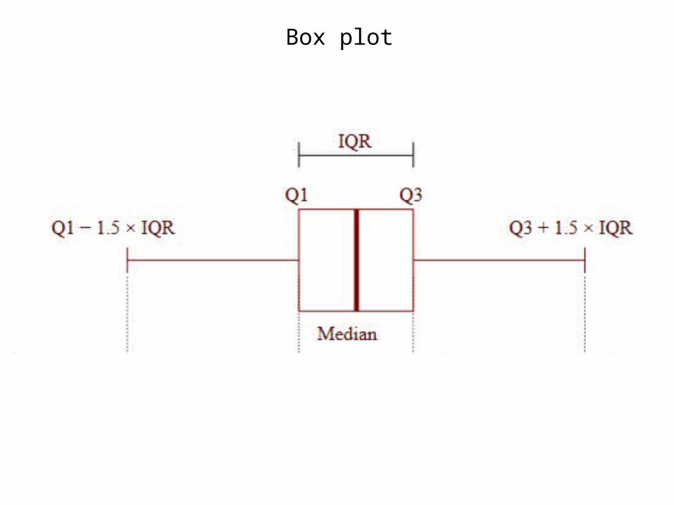
Box plot