Article Electromagnetic Fields of Lightning Return Strokes

Article

Electromagnetic Fields of Lightning Return Strokes-

Revisited

Vernon Cooray 1, and Gerald Cooray2

1Department of Engineering Sciences, Uppsala University, 752 37 Uppsala, Sweden 2Karolinska Institute, Stockholm, Sweden; [email protected]

* Correspondence: [email protected]

Abstract: Electric and/or magnetic fields are generated by stationary charges, uniformly moving

charges and accelerating charges. These field components are described in the literature as static

fields, velocity fields (or generalized Coulomb field) and radiation fields (or acceleration fields),

respectively. In the literature, the electromagnetic fields generated by lightning return strokes are

presented using the field components associated with short dipoles and in this description the one to

one association of the electromagnetic field terms with the physical process that gives rise to them is

lost. In this paper, we will derive expressions for the electromagnetic fields using field equations

associated with accelerating (and moving) charges and separate the resulting fields into static,

velocity and radiation fields. The results illustrates how the radiation fields emanating from the

lightning channel give rise to field terms varying as 1/ r and 21/ r , the velocity fields generating

field terms varying as 21/ r and the static fields generating fields components varying as 21/ r and 31/ r . These field components depend explicitly on the speed of propagation of the current pulse.

However, the total field does not depend explicitly on the speed of propagation of the current pulse.

It is shown that these field components can be combined to generate the field components pertinent

to the dipole technique. However, in this conversion process the connection of the field components

to the physical process taking place at the source that generate these fields (i.e. static charges,

uniformly moving charges and accelerating charges) is lost.

Keywords: Electromagnetic fields, return strokes, dipole fields, accelerating charges, radiation fields,

static fields, velocity fields

1. Introduction

Estimating the field strength and temporal features of electromagnetic fields from lightning

return strokes at a given distance is of interest both in engineering studies, where the protection of

electrical installations from induced voltages from lightning is concerned [1, 2, 3], and in physics

studies, where the properties of lightning return strokes are extracted from the features of

electromagnetic fields measured under conditions where the propagation effects are minimal [4, 5].

The procedure used in these studies is to specify the spatial and temporal variation of the return

stroke current ( , )I z t by appealing to a return stroke model and from that calculating the

electromagnetic fields [6, 7]. Once ( , )I z t is specified, there are four methods to estimate the

electromagnetic fields. Three of these methods, namely, the dipole technique , monopole technique

and the apparent charge density technique are described in [6, 7]. The fourth method, based on the

field equations pertinent to the moving and accelerating charges is described in [8]. For a given ( , )I z t

Preprints (www.preprints.org) | NOT PEER-REVIEWED | Posted: 12 December 2018

© 2018 by the author(s). Distributed under a Creative Commons CC BY license.

Preprints (www.preprints.org) | NOT PEER-REVIEWED | Posted: 12 December 2018 doi:10.20944/preprints201812.0152.v1

© 2018 by the author(s). Distributed under a Creative Commons CC BY license.

mailto:[email protected]

http://creativecommons.org/licenses/by/4.0/

http://dx.doi.org/10.20944/preprints201812.0152.v1

http://creativecommons.org/licenses/by/4.0/

2 of 4

, all these techniques generate the same total electromagnetic fields but the various components that

constitute the total fields differ in different techniques.

The goals of the present paper are the following. First, it is standard practice today to describe

the electromagnetic fields of lightning return stroke in terms of static (field terms decreasing with

distance as 31/ r , where r is the distance from the source to the point of observation), induction (field

terms decreasing with distance as 21/ r ) and radiation (field terms decreasing as1/ r ) [9]. in the

sections to follow we will call these field components dipole-static, dipole-induction and dipole-

radiation. Except in the case of distant radiation fields, this division of the field components cannot

be directly attached to physical processes that generate the electromagnetic fields. In reality there are

only two types of electromagnetic fields. They are the Coulomb and radiation fields. Coulomb fields

are produced by stationary and uniformly moving charges. The Coulomb field produced by

stationary or static charges is called the static field. When the charges are moving the Coulomb field

has to be modified to take into account their motion and this modified field, to separate it from the

static field, is called the velocity field (or generalized Coulomb field). The radiation fields (or

acceleration fields) are produced by accelerating charges. The magnetic field is generated either by

moving charges or by accelerating charges. Thus, the magnetic field is consisted of either the velocity

fields or the radiation fields or both. Unfortunately, when one divides the total field into dipole-static

(i.e. the field components changing as 31/ r ), dipole-induction (i.e. the field components changing as21/ r ) and radiation-dipole (i.e. the field components changing as 1/ r ), as is the standard practice,

except in the case of distant radiation field, the direct association of the field components with the

physical process that generate electromagnetic fields is lost. In this paper we will derive expressions

for the electromagnetic fields of a return stroke where each field component is directly associated

with the physical process that gives rise to it, i.e. stationary charges, moving charges and accelerating

charges. Second, we will show analytically and illustrate it with example, that the resulting field

components can be combined together to produce the field components that are identified in the

literature as dipole-static, dipole-induction and dipole-radiation.

2. Mathematical analysis

Some of the mathematical formulations used in the present paper are identical to those already

presented previously by Cooray and Cooray [10, 11]. For example, the approximations listed in

equations 1 – 11 and the field equations 12 – 23 can be extracted directly from references [10] and [11].

However, since the other equations given in this paper are constructed using these equations, for the

sake of completeness and for easy reference, they are also given here.

The problem under consideration is the calculation of electromagnetic fields from a return stroke

channel when ( , )I z t is specified. The normal procedure of such calculation is to divide the channel

into infinitesimal channel sections of length dz and first estimate the electromagnetic fields from such

a channel element located at height z , where z is the height of the channel element. Once the electric

and magnetic fields produced by this channel element is known, the total field can be obtained by

summing the contributions from all these elements. Let us consider the element dz located at height

z . The first step then is to estimate the electromagnetic fields generated by the said channel element.

For convenience we will treat the problem in frequency domain first and later convert it to time

domain. Assume that the current flowing along the channel element is given by ( ) j ti z e . We consider

the case where this current travels along the channel element with speed u and is absorbed at the other

end of the channel element. In other words, the current that appears at the bottom of the channel

element at any time t will appear at the top of the channel element after a time delay of /dz u . The

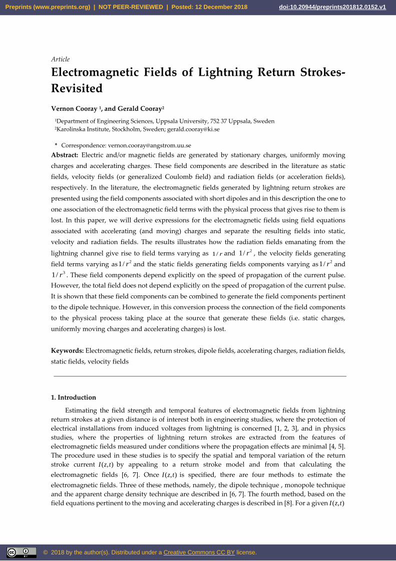
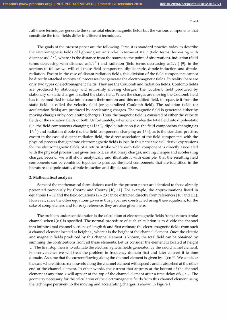
geometry necessary for the calculation of the electromagnetic fields from this channel element using

the technique pertinent to the moving and accelerating charges is shown in Figure 1.

Preprints (www.preprints.org) | NOT PEER-REVIEWED | Posted: 12 December 2018 Preprints (www.preprints.org) | NOT PEER-REVIEWED | Posted: 12 December 2018 doi:10.20944/preprints201812.0152.v1


3 of 4

Figure 1: Geometry, angles and unit vectors pertinent to the evaluation of electromagnetic fields

generated by a channel element. The unit vectora is directed in the direction of the vector

r a a (i.e.

into the paper).

Before we proceed with the analysis let us consider some of the geometrical simplifications that can

be used in the analysis. First of all, we assume that the distance to the point of observation, r , is such

that r dz . When this condition is satisfied one can also make the following simplifications:

1 1( ) = − = sin

2

dz

r

; 2 1( ) = − = sin

2

dz

r

(1)

1cos 1 ; 1cos 1 (2)

1

cos

2

dzr r

= + ;

2

cos

2

dzr r

= − (3)

1

1 1 cos1

2

dz

r r r

= −

;

2

1 1 cos1

2

l

r r r

= +

(4)

2 2

1

1 1 cos1

l

r r r

= −

;

2 2

2

1 1 cos1

l

r r r

= +

(5)

1

cossin sin 1

2

l

r

= −

;

2

cossin sin 1

2

dz

r

= +

(6)

2

1

sincos cos

2

dz

r

= + ;

2

2

sincos cos

2

dz

r

= − (7)

−=−

cos1cos

1 1

c

u

c

u 2sin1

2 1 cos

udz

urc

c

− −

(8)

r

r2

r1

A

B

z



4 of 4

2cos1 1 cos

u u

c c

− = −

2sin1

2 1 cos

udz

urc

c

+ −

(9)

c

u

c

u cos1

1

cos1

1

1 −

=

−

2sin1

2 1 cos

udz

urc

c

+ −

(10)

2

1 1

cos cos11

u u

cc

=

−−

2sin1

2 1 cos

udz

urc

c

− −

(11)

Now, we are in a position to write down the expressions for the electromagnetic fields. The

electromagnetic fields generated by the channel element can be divided into different components as

follows. (a) The electric and magnetic radiation fields generated at the initiation and termination of

the current at the end points of the channel element due to charge acceleration and deceleration,

respectively. (b) The electric and magnetic velocity fields generated by the movement of charges

along the channel element. (c) The static field generated by the accumulation of charges at the two

ends of the channel element. Let us consider these different field components separately. In writing

down these field components, we will depend heavily on the results published previously by Cooray

and Cooray [10, 11]. The field expressions identified by Equations 12 to 23 can be constructed easily

from the results presented in [10].

2.1 Radiation field generated by the charge acceleration and deceleration at the ends of the channel

element

The electric radiation field generated by the initiation of current at the bottom of the channel

element and by the termination of that current at the top of the channel element is given by

1 2

1 2

( / ) ( / / )

1 2

21 2

1 2

sin sin( )

cos cos41 1

j t r c j t l u r c

rad

o

e ei z ud

u ucr r

c c

− − −

= − − −

θ θe a a (12)

The above expression is exact and does not contain any approximations. In order to extract the electric

fields of an infinitesimal current element we will write down the components of this electric field in

the direction of ra and a using the geometrical approximations listed in Equations 1 to 11 which

are valid when r dz . Moreover, we also assume that / 1r c and / 1dz u . Using these

approximations and keeping only the first order terms with respect to dz , the components of this

field in the directions of ra and a become (with /t t r c = − )

,

2

( ) sin

4 (1 cos )

j t

rad

o

i z e ud

uc r

c

=

−

e2cos 2 cos sin

(1 cos )

j dz j dz dz udz

uu c rrc

c

− − + −

θa (13)



5 of 4

2

, 2 2

( ) sin

4(1 cos

j t

rad r r

o

i z e udzd

uc r

c

= −

e a (14)

These two equations define the total radiation field produced by the channel element.

2.2 Velocity field generated by the charges moving from A to B

The velocity field generated as the current pulse propagates along the channel element can be

written as

2 2

2 22 2

2 2

1 1

( ) ( )1 1

4 1 cos 4 1 cos

j t j t

vel

o o

i z e dz u i z e dz ud

c cu ur u r c

c c

= − − −

− −

r ze a a

(15)

The components of this field in the direction of ra and θa after some mathematical manipulations

are given by 2

22

( )1

4 1 cos

j t

vel,r

o

i z e dz ud

u cr u

c

= −

−

re a (16)

2

2 2

2

( ) sin1

4 1 cos

j t

vel,

o

i z e dz ud

cur c

c

= − −

−

θe a

(17)

2.3 Electrostatic field generated by the accumulation of charge at A and B

As the positive current leaves the point A, negative charge accumulates at A and when the

current is terminated at B positive charge is accumulated there. The static Coulomb field produced

by these stationary charges is given by

1 2

2

( / ) ( / / )

2 2

1 2

( )( )

4

j t r c j t dz u r c

stat

o

i z e ed t

j r r

− − − = − −

1r re a a (18)

After using the approximations given earlier, the components of this in the direction of ra and θa

can be written as

, 2

( )

4

j t

stat r

o

i z e dzd

r j

=ecos cosj j

c r u

+ −

ra (19)

, 2

( )( )

4

j t

stat

o

i z e dzd t

r j

=esin

r

θa (20)

2.4 Magnetic radiation field generated during the initiation and termination of the current

The magnetic radiation field generated during the initiation and termination of the current at

the ends of the channel element is given by



6 of 4

1 2( / ) ( / / )

1 2, 3

1 21 2

sin sin( )

cos cos41 1

j t r c j t dz u r c

rad

o

e ei z ud

u ucr r

c c

− − −

= − − −

b a (21)

utilizing the geometrical approximations mentioned earlier and keeping only the second order terms

in dz one obtains

2

, 3

( ) sin 1 cos 2cos sin

cos4(1 cos )1

j t

rad

o

i z e u dz j j ud

uuc r u c rrc

cc

= − − + −−

φb a (22)

2.5 Magnetic velocity field generated as the current pulse propagates along the channel element

The magnetic velocity field generated during the passage of the current along the channel

element is given by

2

2 2

2 2

( ) sin1

4 1 cos

j t

vel,

o

i z e dz ud

cur c

c

= −

−

φb a

(23)

3. Electromagnetic fields of a channel element in time domain

From the frequency domain equations, the time domain equations for the electric and magnetic

fields generated by the channel element can be written directly. The results are the following:

3.1 Radiation fields

, 2

sin( )

4rad

o

dzd t

c r

=E

2 2

2

(z, ) 2 cos sin( , ) ( , )

(1 cos ) (1 cos )

I t u uI z t I z t

u utr rc

c c

− + − −

θa (24)

2

, 2 2

( , ) sin( )

4(1 cos

rad r r

o

I z t dz ud t

uc r

c

= −

E a (25)

, 3

sin( )

4rad

o

dzd t

c r

=B

2 2

2

( , ) 2 cos sin( , ) (z, )

(1 cos ) (1 cos )

I z t u uI z t I t

u utr rc

c c

− + − −

φa (26

3.2 The velocity fields

2

2 2

2

( , ) sin( ) 1

4 1 cos

vel,

o

I z t dz ud t

cur c

c

= −

−

E a (27)



7 of 4

2

22

( )( ) 1

4 1 cosvel,r r

o

I z,t dz ud t

u cr u

c

= −

−

E a (28)

2

2 2

2 2

( ) sin( ) 1

4 1 cos

vel,

o

I z,t dz ud t

cur c

c

= −

−

φB a

(29)

3.3 The Static Fields

, 2( )

4stat r

o

dzd t

r=E

0

cos 1 2cos( , ) ( , ) ( , )

t

I z t I z t I z dc u r

− +

ra (30)

, 2( )

4stat

o

dzd t

r

=E

0

sin( , )

t

I z dr

θa (31)

4. Comparison of the fields of the channel element with fields of a short dipole

The set of equations given in the previous section describe the radiation, velocity and static fields

generated by the channel element. Each of these field terms are associated with the particular process

that generates these fields. Note also that each term is associated with the speed of propagation of

the current pulse. Now, let us sum up the fields in the directions of ra and a without any regard

to the physical mechanism of the field generation. This will generate the following field components

sin( )

4 o

dzd t

=E

2 2 2 2

2 32 3 2 2 2 2 2

0

1 ( , ) 1 (z, ) sin (z, ) 2 cos (z, ) (1 / )( , )

(1 cos ) (1 cos ) (1 cos )

tI z t I t u I t u I t u c

I z du u uc r t r

r c c r crc c c

−

+ + − + − − −

θa (32)

( )4

r

o

dzd t

=E

2 2 2

3 2 22 2 2

0

2cos cos sin (1 / )( , )

(1 cos ) (1 cos )

tI(z,t ) I(z,t ) I(z,t )u I(z,t ) u c

I z du ur r c ur

c r urc c

−

+ − + + − −

ra

(33)

sin( )

4 o

dzd t

=B

2 2 2 2

33 2 2 4 2 2 2 2

1 ( , ) ( , ) 2 cos ( , ) sin ( , ) (1 / )

(1 cos ) (1 cos ) (1 cos )

I z t I z t u I z t u I z t u c

u u uc r tc r r c c r

c c c

−

− + + − − −

a (34)

With some mathematical manipulations one can show that these equations will reduce to (the

mathematical steps necessary for this reduction are given in Appendix A)

sin( )

4 o

dzd t

=E

3 2 2

0

1 ( , ) 1 ( , )( , )

tI z t I z t

I z dr cr c r t

+ +

θa (35)



8 of 4

( )4

r

o

dzd t

=E

3 2

0

2cos 2cos ( , )t

I z tI(z, )d

r r c t

+

ra (36)

sin( )

4 o

dzd t

=B

3 2 2

1 ( , ) ( , )I z t I z t

c r t r c

+

a (37)

The Equations (35), (36) and (37) are identical to the fields of a short dipole [7, 12]. This proves the

equivalence of the dipole technique and the results obtained using equations of accelerating and

moving charges. This equivalence of the two techniques was previously shown for frequency domain

fields in reference [10].

5. The time domain fields of the lightning channel

The electromagnetic fields generated by the lightning channel (without the contribution of the

ground) can be obtained by summing the contributions of all the channel elements located between

0z = to z H= . The results are the following:

5.1 Radiation fields

, 2

0

sin( )

4

H

rad

o

dzt

c r

= E

2 2

2

(z, ) 2 cos sin( , ) ( , )

(1 cos ) (1 cos )

I t u uI z t I z t

u utr rc

c c

− + − −

θa (38)

2

, 2 2

0

( , ) sin( )

4(1 cos )

H

rad r r

o

I z t dz ut

uc r

c

= −

E a (39)

2 2

, 32

0

sin ( , ) 2 cos sin( ) ( , ) (z, )

4(1 cos ) (1 cos )

H

rad

o

dz I z t u ut I z t I t

u uc r tr rc

c c

= − + − −

φB a (40)

5.2 The velocity fields

2

2 2

0 2

( , ) sin( ) 1

4 1 cos

H

vel,

o

I z t dz ut

cur c

c

= −

−

E a (41)

2

220

( )( ) 1

4 1 cos

H

vel,r r

o

I z,t dz ut

u cr u

c

= −

−

E a (42)

2

2 2

0 2 2

( ) sin( ) 1

4 1 cos

H

vel,

o

I z,t dz ut

cur c

c

= −

−

φB a

(43)



9 of 4

5.3 Static Fields

, 2

0

( )4

H

stat r

o

dzt

r= E

0

cos 1 2cos( , ) ( , ) ( , )

t


− +

ra (44)

, 2

0

( )4

H

stat

o

dzt

r

= E

0

sin( , )

t

I z dr

θa (45)

6. Electromagnetic fields of the lightning channel over perfectly conducting ground

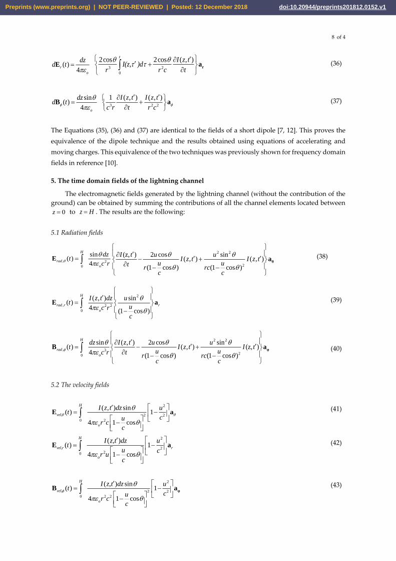
Figure 2: Geometry relevant to the calculation of electromagnetic fields from a return stroke.

The electric field at any point over perfectly conducting ground can be obtained by replacing the

ground plane by an image channel. The relevant geometry is shown in Figure 2. The electric field at

point P located at the surface of the perfectly conducting ground has only a z component and this

field component separated into radiation, velocity and static fields are given by

,z 2

0

( )2

H

rad

o

dzt

c r= −E

2 2 2 4 2

2

(z, )sin 2 sin cos sin cos sin( , ) ( , ) ( , )

(1 cos ) (1 cos ) (1 cos )

I t u u uI z t I z t I z t

u u utr rc

c c c

− + − − − −

za (46)

2 2

2 2

0 2

( , ) sin cos( ) 1

2 1 cos

H

vel

o

I z t dz ut

c u cur c

c

= − − −

−

zE a

(47)

2

0

( )2

H

stat

o

dzt

r= −E 22

0

3sin 2cos cos( , ) ( , ) ( , )

t


− − + −

za (48)

z-axis

Lightning

Channel

r

P

H

z

dz



10 of 4

3

0

sin( )

2

H

rad

o

dzt

c r

= B

2 2

2

( , ) 2 cos sin( , ) (z, )

(1 cos ) (1 cos )

I z t u uI z t I t

u utr rc

c c

− + − −

φa (49)

2

2 2

0 2 2

( ) sin( ) 1

4 1 cos

H

vel

o

I z,t dz ut

cur c

c

= −

−

φB a

(50)

These field expressions can be further simplified as

2

0

( )2

H

rad

o

dzt

c= −E 22 2 4

22

cos sin cos 2(z, )sin ( , ) sin

(1 cos ) (1 cos )

uI t I z t u

u ur t rc

c c

−

+ + − −

za

(51)

2

2

2 2

0 2

( , )( ) 1 cos sin

2 1 cos

H

vel

o

I z t dz ut

cur c

c

= − − −

−

zE a

(52)

0

( )2

H

stat

o

dzt

= −E 2

2 3

0

3sin 2cos1 cos ( , ) ( , )

tu

I z t I z dur c r

− − −

za (53)

3

0

sin( )

2

H

rad

o

dzt

c

= B

2

( , ) ( , ) sin2cos

(1 cos ) (1 cos )

I z t uI z t u

u ur tr c

c c

− − − −

φa

(54)

2

2 2

0 2 2

( ) sin( ) 1

4 1 cos

H

vel

o

I z,t dz ut

cur c

c

= −

−

φB a

(55)

Based on the analysis presented in section 4 these field terms can be reduced to dipole fields resulting

in

2

0

( )2

H

rad

o

dzt

c= −E

2 2 22

2 3

0

3sin 2 ( , ) 3sin 2(z, )sin( , )

tc I z t cI tI z d

r t r r

− − + +

za (56)

3

0

sin( )

2

H

rad

o

dzt

c

= B

2

( , ) ( , )I z t cI z t

r t r

+

φa (57)

In order to illustrate this point further let us consider the electric fields generated by a lightning return

stroke as simulated using the Modified Transmission Line model with Exponential current

attenuation (MTLE) [13]. The spatial and temporal distribution of the current, ( , )I z t , associated with

this model are given by



11 of 4

( , ) 0I z t = /t z u (58)

/( , ) (0, )zI z t e I t−= /t z u (59)

In the above equations, z is the height of the point of observation along the vertical channel, is the

current decay height constant, u is the speed of propagation of the return stroke front and (0, )I t is the

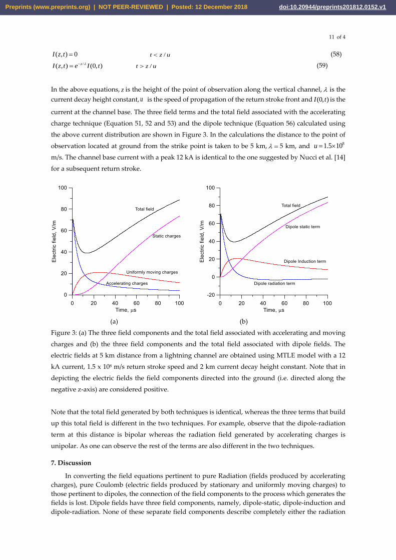
current at the channel base. The three field terms and the total field associated with the accelerating

charge technique (Equation 51, 52 and 53) and the dipole technique (Equation 56) calculated using

the above current distribution are shown in Figure 3. In the calculations the distance to the point of

observation located at ground from the strike point is taken to be 5 km, = 5 km, and 81.5 10u =

m/s. The channel base current with a peak 12 kA is identical to the one suggested by Nucci et al. [14]

for a subsequent return stroke.

(a) (b)

Figure 3: (a) The three field components and the total field associated with accelerating and moving

charges and (b) the three field components and the total field associated with dipole fields. The

electric fields at 5 km distance from a lightning channel are obtained using MTLE model with a 12

kA current, 1.5 x 108 m/s return stroke speed and 2 km current decay height constant. Note that in

depicting the electric fields the field components directed into the ground (i.e. directed along the

negative z-axis) are considered positive.

Note that the total field generated by both techniques is identical, whereas the three terms that build

up this total field is different in the two techniques. For example, observe that the dipole-radiation

term at this distance is bipolar whereas the radiation field generated by accelerating charges is

unipolar. As one can observe the rest of the terms are also different in the two techniques.

7. Discussion

In converting the field equations pertinent to pure Radiation (fields produced by accelerating

charges), pure Coulomb (electric fields produced by stationary and uniformly moving charges) to

those pertinent to dipoles, the connection of the field components to the process which generates the

fields is lost. Dipole fields have three field components, namely, dipole-static, dipole-induction and

dipole-radiation. None of these separate field components describe completely either the radiation



12 of 4

(fields generated by accelerating charges), velocity or static field components (Coulomb fields). Of

course, the distant radiation-dipole field describe the energy radiated to infinity by the accelerating

charges. But, this is not the only field component that is being produced by accelerating charges. The

dipole-static term describes only part of the static field, the dipole-induction field is a combination of

static, velocity and radiation terms and dipole-radiation field describe only part of the radiation field.

Note that pure radiation field has terms both varying as1/ r and 21/ r .

It is important to point out that not only the 1/ r field terms that carry energy from one place

to another. The field terms varying as 21/ r terms also do that. The difference is that while1/ r

terms carry energy to infinity the 21/ r terms carry energy into space in the vicinity of the dipole. As

the current flows along the channel, charges are transported along it and these displaced charges

generate electric fields in space. These electric fields (and also magnetic fields) carry energy and it is

the 21/ r terms that supply this energy. However, if the displaced charges reunite by coming back to

the original location, these field components will transport this energy, located in space, back to the

source. That means the flow of energy caused by these 21/ r terms can change direction when the

current flowing along the channel reverses its direction of flow or polarity. Indeed, in the case of

oscillating dipoles these terms carry energy back and forth from the source to space and vice-versa.

Observe that, even though the radiation, velocity and the static fields of a channel element

depend explicitly on the speed of propagation of the current pulse (i.e. Equations 24 to 31) the total

field is independent of the speed of propagation (Equations, 35, 36 and 37). Thus, the speed of

propagation enters into the electromagnetic fields of the channel element only if we wish to separate

the total field into its physical constituents. This also shows that if the speed of propagation of the

pulse travelling along the channel element is changed, the total field remains the same while the three

components that constitute the field will change. However, the situation is different when one

constructs the return stroke field by summing up the contributions from all the channel elements.

Since the time delays between the fields from different channel elements depend on the return stroke

speed, the sum of the fields from all the channel elements depends on the return stroke speed. Thus,

the three components of the return stroke field as well as the total field depend on the return stroke

speed.

Finally, note that the total field calculated for a channel element or a lightning return stroke is

the same irrespective of whether the equations pertinent to accelerating charges or the dipole

equations are used. Even though, this point was demonstrated numerically in previous publications

[3], it was demonstrated analytically in the present paper.

8. Conclusion

In this paper we have presented analytical expressions for the electromagnetic fields generated

by return strokes in terms of the field components generated by accelerating charges, moving charges

and stationary charges. It is shown analytically and demonstrated using return stroke fields that these

three field components can be reduced to those of the field expressions pertinent to the dipole

technique but in the reduction process the association of the individual field components to the

physical processes that generate the electromagnetic fields is lost.



13 of 4

Appendix A: Mathematical steps necessary for the reduction of electromagnetic fields obtained

from accelerating and moving charges to the dipole fields.

(a) Reduction of d E to the dipole fields:

The mathematical steps necessary for the reduction starting from Equation (32) are shown

below.

sin( )

4 o

dzd t

=E

2 2 2 2

2 32 3 2 2 2 2 2

0

1 ( , ) 1 (z, ) sin (z, ) 2 cos (z, ) (1 / )( , )

(1 cos ) (1 cos ) (1 cos )

ti z t i t u i t u i t u c

I z du u uc r t r

r c c r crc c c

−

+ + − + − − −

θa (a1)

Let us combine the third and fifth terms inside the bracket. The result is given by

sin( )

4 o

dzd t

=E

2 2 2

2 3 2 22 2 2 2

0

1 ( , ) 1 (z, ) sin (z, ) 2 cos( , ) 1

(1 cos ) (1 cos )

ti z t i t u u i t u

I z du uc r t r c c

r c c rc c

+ + + − − − −

θa (a2)

sin( )

4 o

dzd t

=E

2 2 2 2

2 3 2 2 22 2 2 2

0

1 ( , ) 1 (z, ) cos (z, ) 2 cos( , ) 1

(1 cos ) (1 cos )

ti z t i t u u u i t u

I z du uc r t r c c c

r c c rc c

+ + − + − − − −

θa (a3)

sin( )

4 o

dzd t

=E

2 2

2 3 22 2 2 2

0

1 ( , ) 1 (z, ) cos (z, ) 2 cos( , ) 1

(1 cos ) (1 cos )

ti z t i t u i t u

I z du uc r t r c

r c c rc c

+ + − − − −

θa (a4)

sin( )

4 o

dzd t

=E

2 3

2 2 2 20

1 ( , ) 1 (z, ) (z, ) 2 cos( , ) (1 cos )(1 cos )

(1 cos ) (1 cos )

ti z t i t u u i t u

I z du uc r t r c c

r c c rc c

+ + − + − − −

θa (a5)

sin( )

4 o

dzd t

=E



14 of 4

2 3

2 2 20

(z, )(1 cos )1 ( , ) 1 (z, ) 2 cos

( , )

(1 cos ) (1 cos )

tu

i ti z t i t ucI z d

u uc r t rr c c r

c c

+

+ + − − −

θa (a6)

sin( )

4 o

dzd t

=E

2 32

0

1 ( , ) 1 (z, ) 2 cos( , ) 1 cos

(1 cos )

ti z t i t u u

I z duc r t r c c

r cc

+ + + − −

θa (a7)

sin( )

4 o

dzd t

=E

2 32

0

1 ( , ) 1 (z, )( , ) 1 cos

(1 cos )

ti z t i t u

I z duc r t r c

r cc

+ + − −

θa (a8)

sin( )

4 o

dzd t

=E

2 3 2

0

1 ( , ) 1 (z, )( , )

ti z t i t

I z dc r t r r c

+ +

θa (a9)

(b) Reduction ofrdE to the dipole fields:


below.

( )4

r

o

dzd t

=E

2 2 2

3 2 22 2 20

2cos cos sin (1 /( , )

1 cos 1 cos

ti(z,t ) i(z,t ) i(z,t )u i(z,t ) u c

i z du ur r c ur

c r urc c

−

+ − + + − −

ra (a10)

( )4

r

o

dzd t

=E

2 2 2 2

3 220

2cos ( , ) cos sin (1 / )( , ) 1

1 cos 1 cos

ti z t u u u c

i z du ur ur c

cc c

−

+ − + + − −

ra (a11)

( )4

r

o

dzd t

=E ( )2 2 2 2

3 220

2cos ( , ) cos 1( , ) 1 sin

1 cos

ti z t u

i z d u c uur ur c

cc

+ − + + − −

ra (a12)

( )4

r

o

dzd t

=E ( )2 2 2

3 220

2cos ( , ) cos 1( , ) 1 cos

1 cos

ti z t u

i z d c uur ur c

cc

+ − + − −

ra (a13)

( )4

r

o

dzd t

=E

22

3 2 2

0

2cos ( , ) cos 1( , ) 1 1 cos

1 cos

ti z t u u

i z dur ur c c

c

+ − + − −

ra (a14)



15 of 4

( )4

r

o

dzd t

=E

3 2

0

2cos ( , ) cos cos( , ) 1 1

ti z t u u

i z dr ur c c

+ − + +

ra (a15)

( )4

r

o

dzd t

=E

3 2

0

2cos ( , ) 2 cos( , )

ti z t u

i z dr ur c

+

ra (a16)

(c) Reduction of d B to the dipole fields:


below.

sin( )

4 o

dzd t

=B

2 2 2 2

33 2 2 4 2 2 2 2

1 ( , ) ( , ) 2 cos ( , ) sin ( , ) (1 / )

(1 cos ) (1 cos ) (1 cos )

i z t i z t u i z t u i z t u c

u u uc r tc r r c c r

c c c

−

− + + − − −

a (a17)

sin( )

4 o

dzd t

=B

2 22

3 2 23 2 2 2 2

1 ( , ) ( , ) 2 cos ( , )sin (1

(1 cos ) (1 cos )

i z t i z t u i z t u u

u uc r t c cc r r c

c c

− + + − − −

a (a18)

sin( )

4 o

dzd t

=B

22

3 23 2 2 2 2

1 ( , ) ( , ) 2 cos ( , )1 cos

(1 cos ) (1 cos )

i z t i z t u i z t u

u uc r t cc r r c

c c

− + − − −

a (a19)

sin( )

4 o

dzd t

=B

33 2 2 2

1 ( , ) ( , ) 2 cos ( , )1 cos

(1 cos ) (1 cos )

i z t i z t u i z t u

u uc r t cc r r c

c c

− + + − −

a (a20)

sin( )

4 o

dzd t

=B

32 2

1 ( , ) ( , ) 21 cos cos

(1 cos )

i z t i z t u u

uc r t c cc r

c

+ + − −

a (a21)

sin( )

4 o

dzd t

=B

3 2 2

1 ( , ) ( , )i z t i z t

c r t c r

+

a (a22)

Author Contributions: Vernon Cooray conceived the idea; Both authors contributed equally in the analysis

and in writing the paper.

Funding: This work was supported by Swedish Research Council grant VR-2015-05026 and partly by the fund

from the B. John F. and Svea Andersson donation at Uppsala University.

Conflicts of Interest: The authors declare no conflict of interest.

References

1. F. Rachidi, "A review of field-to-transmission line coupling models with special emphasis to

lightning-induced voltages", IEEE Trans. Electromagn. Compat., vol. 54, no. 4, pp. 898-911,

Aug. 2012.



16 of 4

2. C. A. Nucci, F. Rachidi, M. Rubinstein, "Interaction of lightning-generated electromagnetic

fields with overhead and underground cables Chapter 18 of Lightning Electromagnetics

(Edited by Cooray), IET, pp. 678-718, 2012.

3. Baba, Y. and V. Rakov, Voltages Induced on an Overhead Wire by Lightning Strikes to a

Nearby Tall Grounded Object, IEEE Trans. Electromagn. Compat.,, Vol. 48, No. 1, 212 – 224,

2006.

4. Ye, M. and V. Cooray, Propagation effects caused by a rough ocean surface on the

electromagnetic fields generated by lightning return strokes, Radio Sci., vol. 29, 73 - 85, 1994.

5. Cooray, V., and Ye. Ming, Propagation effects on the lightning generated electromagnetic

fields for homogeneous and mixed sea land paths, J. Geophys. Res., vol. 99, 10641 - 10652,

1994.

6. Thottappillil, R., and V.A. Rakov, On different approaches to calculating lightning electric

fields, Journal of Geophysical Research, 106, 14191-14205, 2001.

7. Thottappillil, R., Computation of electromagnetic fields from lightning discharges, in The

Lightning Flash (second edition), edited by V. Cooray, IET publishers, London, 2014.

8. Cooray, V. and Cooray, G., The electromagnetic fields of an accelerating charge:

Applications in lightning return stroke models, Trans. IEEE (EMC), in Press, 2010.

9. McLain, D. K. and M. A. Uman, Exact expression and moment approximation for the electric

field intensity of the lightning return stroke, J. Geophys. Res., vol. 76, pp. 2101–2105, 1971.

10. Cooray, G. and V. Cooray, Electromagnetic fields of a short electric dipole in free space –

revisited, Progress in Electromagnetic Research, vol. 131, 357-373, 2012.

11. Cooray, V., Application of electromagnetic fields of an accelerating charge to obtain the

electromagnetic fields of a propagating current pulse, in The Lightning Electromagnetics,

edited by V. Cooray, IET publishers, London, 2012.

12. Pannofsky, W. K. H. and M. Phillips, Classical Electricity and Magnetism, Addison-Wesley,

Reading, Mass, 1962.

13. Nucci, C. A., C. Mazzetti, F. Rachidi and M. Ianoz, On lightning return stroke models for

LEMP calculations,” in 19th Int. Conf. Lightning Protection, Graz, Austria, 1988.

14. Nucci, C. A., G. Diendorfer, M. A. Uman, F. Rachidi, M. Ianoz, C. Mazetti, Lightning return

stroke models with specified channel base current: A review and comparison, J. Geophys.

Res., 95, 20395-20408, 1990.



Documents

Article Electromagnetic Fields of Lightning Return Strokes