Embed Size (px)
Citation preview
Energies 2021, 14, 5641. https://doi.org/10.3390/en14185641 www.mdpi.com/journal/energies
Article
Effect of Individual Volt/var Control Strategies
in LINK‐Based Smart Grids with a High Photovoltaic Share
Daniel‐Leon Schultis * and Albana Ilo
Institute of Energy Systems and Electrical Drives, TU Wien, 1040 Vienna, Austria; [email protected]
* Correspondence: daniel‐[email protected]
Abstract: The increasing share of distributed energy resources aggravates voltage limit compliance
within the electric power system. Nowadays, various inverter‐based Volt/var control strategies,
such as cosφ(P) and Q(U), for low voltage feeder connected L(U) local control and on‐load tap
changers in distribution substations are investigated to mitigate the voltage limit violations caused
by the extensive integration of rooftop photovoltaics. This study extends the L(U) control strategy
to X(U) to also cover the case of a significant load increase, e.g., related to e‐mobility. Control en‐
sembles, including the reactive power autarky of customer plants, are also considered. All Volt/var
control strategies are compared by conducting load flow calculations in a test distribution grid. For
the first time, they are embedded into the LINK‐based Volt/var chain scheme to provide a holistic
view of their behavior and to facilitate systematic analysis. Their effect is assessed by calculating the
voltage limit distortion and reactive power flows at different Link‐Grid boundaries, the correspond‐
ing active power losses, and the distribution transformer loadings. The results show that the control
ensemble X(U) local control combined with reactive power self‐sufficient customer plants performs
better than the cosφ(P) and Q(U) local control strategies and the on‐load tap changers in distribution
substations.
Keywords: Volt/var control; distribution grid; photovoltaic; smart grid; LINK; boundary voltage
limits; local control; X(U); CP_Q‐Autarky
1. Introduction
Voltage is one of the basic quality parameters of power systems with limits specified
in grid codes [1]. The massive connection of renewable and distributed generation and
the increasing electricity demand aggravate compliance to the voltage limits, especially in
the radial structures of distribution grids. Active and reactive power flows in these grids,
as well as the transformers’ tap positions, affect the voltages. However, active power is
the only product of the power industry that, as a consequence, should not be used for
voltage control, even in grids with an R/X ratio greater than 1. On the contrary, reactive
power is a by‐product of AC systems proven to have an essential effect on voltages. There‐
fore, controlling reactive power and on‐load tap changers (OLTC) through a Volt/var con‐
trol (VvC) process is feasible to maintain acceptable voltages within the distribution grid.
Many distributed energy resources (DER) can participate in the VvC process by contrib‐
uting reactive power [2]. Today, local controls are mainly used to utilize their var capa‐
bilities across all power system levels.
Rooftop photovoltaic (PV) inverters, installed at the customer plant (CP) level, are
commonly equipped with cosφ(P) and Q(U) controls [3], or more sophisticated strategies
[4–8], in order to mitigate voltage limit violations at the low voltage (LV) level. These
control strategies may also be applied to electric vehicle (EV) chargers [9,10]. However,
the distributed nature of CPs weakens the effectiveness of these control strategies [11],
Citation: Schultis, D.‐L.; Ilo, A. Effect of
Individual Volt/Var Control Strategies
in LINK‐Based Smart Grids with a
High Photovoltaic Share.
Energies 2021, 14, 5641.
https://doi.org/10.3390/en14185641
Academic Editor: Luis Hernández‐
Callejo
Received: 18 August 2021
Accepted: 6 September 2021
Published: 8 September 2021
Publisher’s Note: MDPI stays neu‐
tral with regard to jurisdictional
claims in published maps and institu‐
tional affiliations.
Copyright: © 2021 by the authors. Li‐
censee MDPI, Basel, Switzerland.
This article is an open access article
distributed under the terms and con‐
ditions of the Creative Commons At‐
tribution (CC BY) license (http://crea‐
tivecommons.org/licenses/by/4.0/).
Energies 2021, 14, 5641 2 of 31
making active power curtailment necessary in many cases [12]. The use of customers’ ap‐
pliances to control the voltage in LV grids provokes social issues concerning data privacy
and discrimination [13], contradicting the political intentions of the European Parliament
[14,15]. As an alternative, local Volt/var control may be realized directly at the LV level.
Some research projects have upgraded distribution transformers with OLTCs [16]. OLTCs
are slow to operate and are sensitive to the number of tap operations. They cannot react
appropriately to the voltage fluctuations caused by the intermittent PV injections. Tem‐
porary voltage limit violations and unnecessary tap operations are thus a consequence,
jeopardizing the electrical equipment and shortening the transformers’ durability [17].
Reference [18] proposes a Volt/var control ensemble, where L(U) controlled inductive de‐
vices installed close to the ends of the violating LV feeders control the voltage locally, and
the PV inverters supply the reactive power demand of the CPs. However, the increasing
electricity demand, which is mainly due to the electrification of the heat and transporta‐
tion sector [19], may provoke violations of the lower voltage limit that the inductive de‐
vices cannot mitigate. The OLTCs supplying substations control the voltage at the me‐
dium voltage (MV) level. In some cases, additional capacitor banks are used to support
voltage control for long feeders [20].
The uncontrolled reactive power flows provoked by local VvCs in the radial struc‐
tures of distributed grids constitute a significant concern for future smart grids [21]—
transmission (TSO) and distribution system operators (DSO) are experiencing substantial
operational challenges [22,23]. The use of modern information and communication tech‐
nologies (ICT) to automatically optimize, protect, and monitor the operation of the com‐
plete power system, including CPs [24], does not meet the rigorous cyber‐security and
data privacy requirements [25].
Completing all technical and market‐related aspects by meeting today’s data protec‐
tion and cyber security requirements requires a holistic view of smart grids [26]. The LINK
architecture provides a holistic solution for smart grids, enabling the execution of various
operation processes, such as demand response, static and dynamic stability, generation
load balance, and monitoring [26,27]. It divides the power system into chains of grid‐,
producer‐, and storage‐links, which fit one into another to establish flexible and reliable
electrical connections [28]. The standardized structure of LINK‐based smart grids allows
for realizing the Volt/var process in the horizontal and vertical axes as chain controls that
minimize the necessary data exchanges [29]. While the horizontal axis includes the inter‐
connected high voltage (HV) grids, the vertical ones contain all system levels, i.e., HV,
MV, LV, and CP levels [30].
Numerous studies have been conducted to analyze the effects of different Volt/var
control strategies on the behavior of LV grids using load flow simulations [13,31–34].
These studies calculate the grid state for a specified voltage at the slack node, but do not
analyze the impact of Volt/var control on the boundary voltage limits (BVL) at the distri‐
bution and supplying substation levels [35] for different local control strategies such as
cosφ(P), Q(U), and OLTC in distribution transformers. This paper upgrades the L(U) local
control strategy to X(U), supporting the increase in electricity demand, e.g., due to e‐mo‐
bility. The LINK architecture [28] is used to analyze the impact of various Volt/var control
strategies on the voltage limits at different system boundaries, such as LV−MV and
MV−HV. All control setups are embedded into the LINK‐based Volt/var control chain
scheme.
Section 2 describes the materials and methods used, including the methodology, gen‐
eralized Volt/var chain control, test grids, and control setups. The results are presented in
Section 3. In Section 4, the effects of the different control setups are compared and dis‐
cussed. Finally, conclusions are drawn in Section 5.
2. Materials and Methods
2.1. Methodology
Energies 2021, 14, 5641 3 of 31
2.1.1. Investigation Methodology
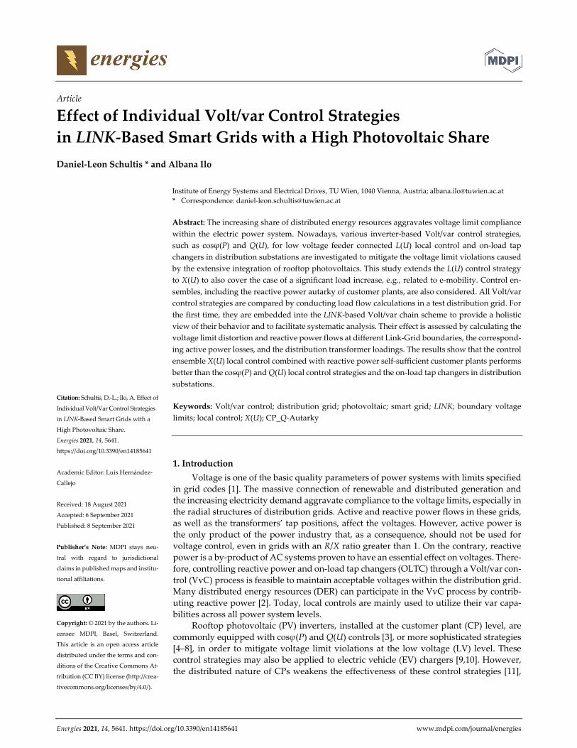
Figure 1 shows the methodology used to investigate the effects of the individual con‐
trol strategies. The state‐of‐the‐art and newly introduced local control strategies are em‐
bedded into the LINK‐based Volt/var control process. Possible control ensembles, i.e.,
combinations of local controls at the LV level with the Q‐Autarkic operation mode of cus‐
tomer plants, are identified. Load flow simulations are conducted in an exemplary vertical
link chain, including the MV, LV, and CP levels, to quantify the effects of various control
arrangements on the grid behavior.
Figure 1. Methodology used to investigate the effects of individual control strategies in the LINK‐based Volt/var control process.
2.1.2. Modeling Procedure
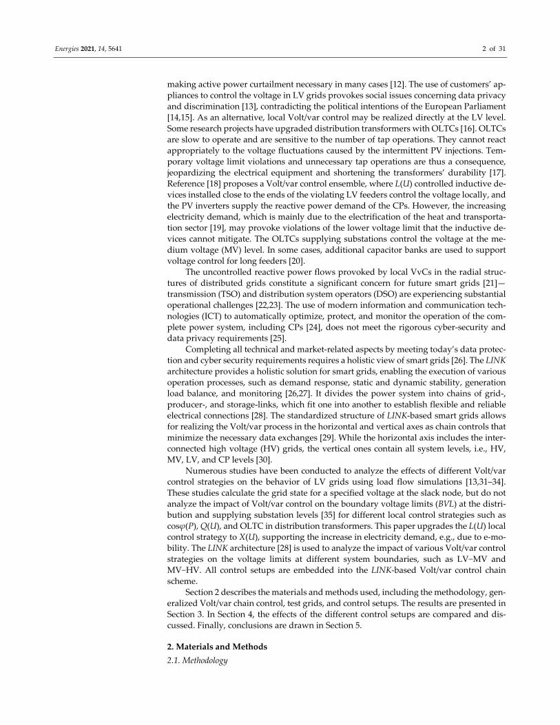
The LINK‐based chain modeling procedure, introduced in [35] and overviewed in
Figure 2, is used to calculate the test grids’ behavior for different Volt/var control arrange‐
ments. In contrast with conventional load modeling, this approach uses the BVL‐concept
to validate voltage limit compliance throughout the entire Smart Grid through separate
analysis of each system level. Joint modeling and analysis of MV and LV grids are not
necessary. First, the lumped CP models are created by specifying their P(U) and Q(U)
behavior and setting their boundary voltage limits to conform to the Grid Code. The
lumped CP models are used to calculate the P(U) and Q(U) behavior and the boundary
voltage limits at the distribution substation via load flow simulations, yielding the lumped
LV grid models. Finally, load flow simulations are conducted at the MV level to identify
the behavior and boundary voltage limits at the supplying substation. Their lumped mod‐
els represent the connected LV grids and CPs. This calculation procedure is repeated for
different Volt/var control arrangements to investigate their impact on the system behav‐
ior.
Figure 2. Overview of the LINK‐based chain modeling procedure used to analyze the behavior of the test grids at distri‐
bution and supplying substations.
2.2. Generalized Vertical Volt/var Chain Control Scheme
LINK architecture arranges Volt/var chain control schemes in the horizontal and vertical
power system axes. The focus of this study is set on the vertical Volt/var chain control scheme.
It involves primary (PC), Direct (DiC), and secondary controls (SC) (see Appendix A) to main‐
tain the voltage limit compliance throughout the entire smart grid by coordinating the
reactive power flows with the on‐load tap changers. Local controls (LC) may also be inte‐
grated.
Figure 3 shows the generalized form of the vertical Volt/var chain control wherein
the grid‐links are set according to HV, MV, LV, and CP levels. While the automation and
communication path is drawn in blue, the power flow path is black. One of the evolution‐
ary discoveries of the LINK solution is the grid identification within the customer plants
and its consideration in the design of the holistic architecture [28]. The underpinned wires

Energies 2021, 14, 5641 4 of 31
between the meter and the various sockets and electrical devices constitute a radial grid.
The grid‐link size is variable and is determined by the area where the corresponding SC
is set up. It may be applied separately to each classical level of the grid and to a part that
includes more than one level, e.g., MV and LV. Each grid‐link includes electrical appli‐
ances, i.e., lines/cables, transformers, and reactive power devices (RPD); the Volt/var sec‐
ondary control (VvSC); and interfaces to the neighboring grid‐, producer‐ and storage‐
links.
The entirety of all electrical appliances included in a grid‐link is denoted as the “Link‐
Grid”. Link‐Grids are interconnected via boundary link nodes (BLiN), and the producer‐
and storage‐links are connected to the Link‐Grids via boundary producer (BPN) and
boundary storage nodes (BSN). Besides the electrical appliance, each producer‐ and stor‐
age‐link includes a PC and an interface to the corresponding SC. In its generalized form,
the Volt/var chain control utilizes all reactive power resources, including storages with
reactive power capabilities, across all system levels. The neighboring grid‐links may act
as additional control variables by accepting reactive power set‐points and considering
them as constraints.
Figure 3. Overview of the generalized vertical Volt/var chain control.
Equation (1) compactly represents the control variables and dynamic constraints of
the vertical Volt/var chain control, considering the MV, LV, and CP levels. Three VvSCs
are involved that calculate the set‐points for the corresponding control variables, which
are put in parentheses.
𝑉𝑣𝑺𝑪 𝑉𝑣𝑺𝑪 𝑷𝑪 ,𝑷𝑪 ,𝑷𝑪 ,𝑷𝑪 , 𝑫𝒊𝑪 ,𝑺𝑪 ,𝑺𝑪 ; 𝑪𝒏𝒔 ,
𝑉𝑣𝑺𝑪 𝑷𝑪 ,𝑷𝑪 , 𝑷𝑪 ,𝑷𝑪 ,𝑫𝒊𝑪 ,𝑺𝑪 ; 𝑪𝒏𝒔 ,
𝑉𝑣𝑺𝑪 𝑷𝑪 ,𝑷𝑪 ,𝑷𝑪 ,𝑫𝒊𝑪 ; 𝑪𝒏𝒔
(1)
At the medium voltage level, 𝑉𝑣𝑺𝑪 calculates the following:
The voltage set‐points for the primary controls 𝑷𝑪 of the supplying transform‐
ers and other transformers included in the MV_Link‐Grid that have OLTC;
The voltage and reactive power set‐points for the primary controls 𝑷𝑪 of the pro‐
ducer‐links connected to the MV_ Link‐Grid;
The voltage and reactive power set‐points for the primary controls 𝑷𝑪 of the stor‐
age‐links connected to the MV_ Link‐Grid;
The voltage, reactive power, and switch position set‐points for the primary 𝑷𝑪
and direct controls 𝑫𝒊𝑪 of the RPDs included in the MV_ Link‐Grid;
Energies 2021, 14, 5641 5 of 31
The reactive power set‐points for the secondary controls 𝑺𝑪 of the neighboring
CP_Grid‐Links; and
The reactive power set‐points for the secondary controls 𝑺𝑪 of the neighboring
LV_Grid‐Links;
While respecting the following:
The reactive power constraint 𝑪𝒏𝒔 at the boundary node to the neighboring
HV_ Link‐Grid.
At the low voltage level, 𝑉𝑣𝑺𝑪 calculates the following:
The voltage set‐points for the primary control 𝑷𝑪 of the distribution transformer
included in the LV_Link‐Grid (when it possesses an OLTC);
The voltage and reactive power set‐points for the primary controls 𝑷𝑪 of the pro‐
ducer‐links connected to the LV_Link‐Grid;
The voltage and reactive power set‐points for the primary controls 𝑷𝑪 of the stor‐
age‐links connected to the LV_Link‐Grid;
The voltage, reactive power, and switch position set‐points for the primary 𝑷𝑪
and direct controls 𝑫𝒊𝑪 of the RPDs included in the LV_Link‐Grid; and
The reactive power set‐points for the secondary controls 𝑺𝑪 of the neighboring
CP_Grid‐Links;
While respecting the following:
The reactive power constraints 𝑪𝒏𝒔 at the boundary node to the neighboring
MV_Link‐Grid.
At the customer plant level, 𝑉𝑣𝑺𝑪 calculates the following:
The voltage and reactive power set‐points for the primary controls 𝑷𝑪 of the pro‐
ducer‐links connected to the CP_Link‐Grid;
The voltage and reactive power set‐points for the primary controls 𝑷𝑪 of the stor‐
age‐links connected to the CP_Link‐Grid; and
The switch position set‐points for the primary 𝑷𝑪 and direct controls 𝑫𝒊𝑪 of
the RPDs included in the CP_Link‐Grid;
While respecting the following:
The reactive power constraint 𝑪𝒏𝒔 at the boundary node to the neighboring
LV_Link‐Grid.
2.3. Description of Test Link‐Grids
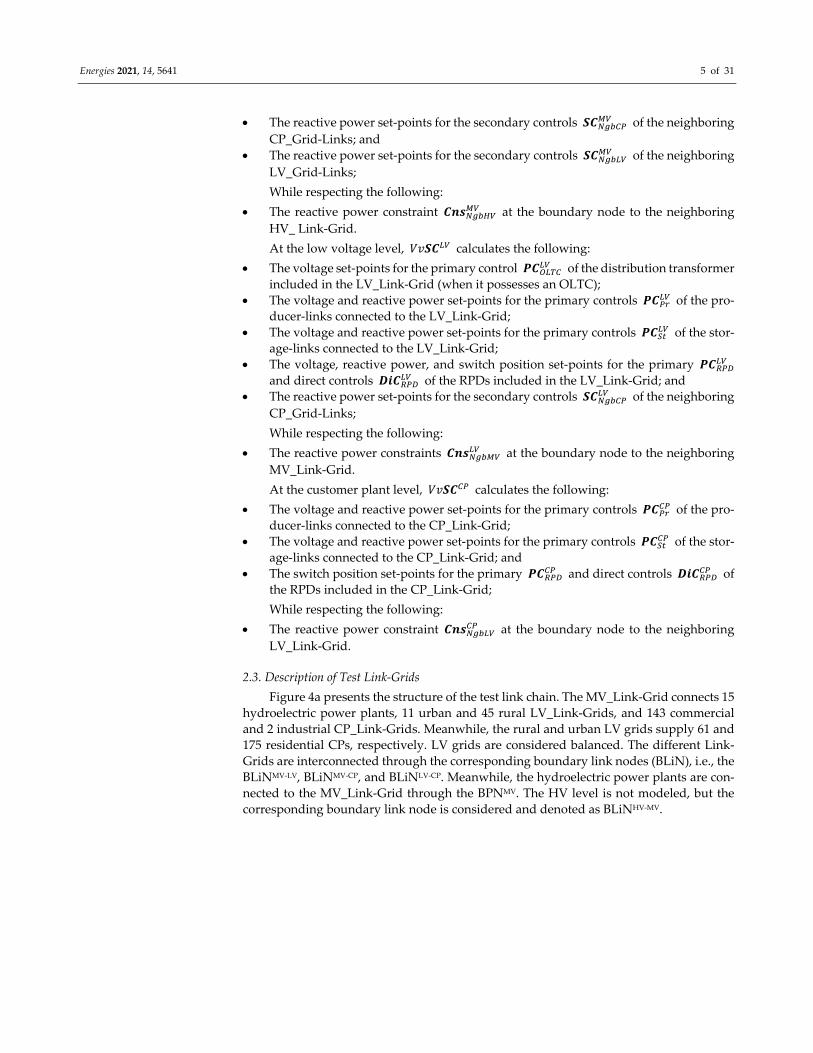
Figure 4a presents the structure of the test link chain. The MV_Link‐Grid connects 15
hydroelectric power plants, 11 urban and 45 rural LV_Link‐Grids, and 143 commercial
and 2 industrial CP_Link‐Grids. Meanwhile, the rural and urban LV grids supply 61 and
175 residential CPs, respectively. LV grids are considered balanced. The different Link‐
Grids are interconnected through the corresponding boundary link nodes (BLiN), i.e., the
BLiNMV‐LV, BLiNMV‐CP, and BLiNLV‐CP. Meanwhile, the hydroelectric power plants are con‐
nected to the MV_Link‐Grid through the BPNMV. The HV level is not modeled, but the
corresponding boundary link node is considered and denoted as BLiNHV‐MV.

Energies 2021, 14, 5641 6 of 31
(b)
(c)
(a) (d)
Figure 4. Structure of the test link chain: (a) overview; (b) residential CP_Link‐Grids; (c) rural LV_Link‐Grid; (d) MV_Link‐Grid.
2.3.1. Customer Plant Level
Four different types of CP_Link‐Grids are considered: rural and urban residential,
commercial, and industrial. Only the former is described in detail, while the others are
documented in Appendix B. The voltage limits at the BLiNLV‐CP are set to 0.9 and 1.1 p.u.
and conform to the German Grid Code [36]. The corresponding active (𝑃 ) and reac‐
tive power flows (𝑄 ) are determined by three model components: equivalent con‐
suming device (Dev.‐model), producer (Pr.‐model), and storage model (St.‐model; Figure
4b). The underpinned wires at the CP level are neglected. Figure 5 shows the load and
production profiles of these model components, which have a resolution of 10 min.
(a) (b) (c)
Figure 5. Load and production profiles of different model components of the rural residential CP_Link‐Grid: (a) Dev.‐
model; (b) Pr.‐model; (c) St.‐model.
All consuming devices, such as switch‐mode power supply, resistive, and lighting
devices, as well as motors, are represented by the Dev.‐model. Equation (2) determines
the voltage‐dependent active (𝑃 ) and reactive power contributions (𝑄 ) , using
the load profiles and time‐variant ZIP‐coefficients from [37]. The load profiles reflect the
Energies 2021, 14, 5641 7 of 31
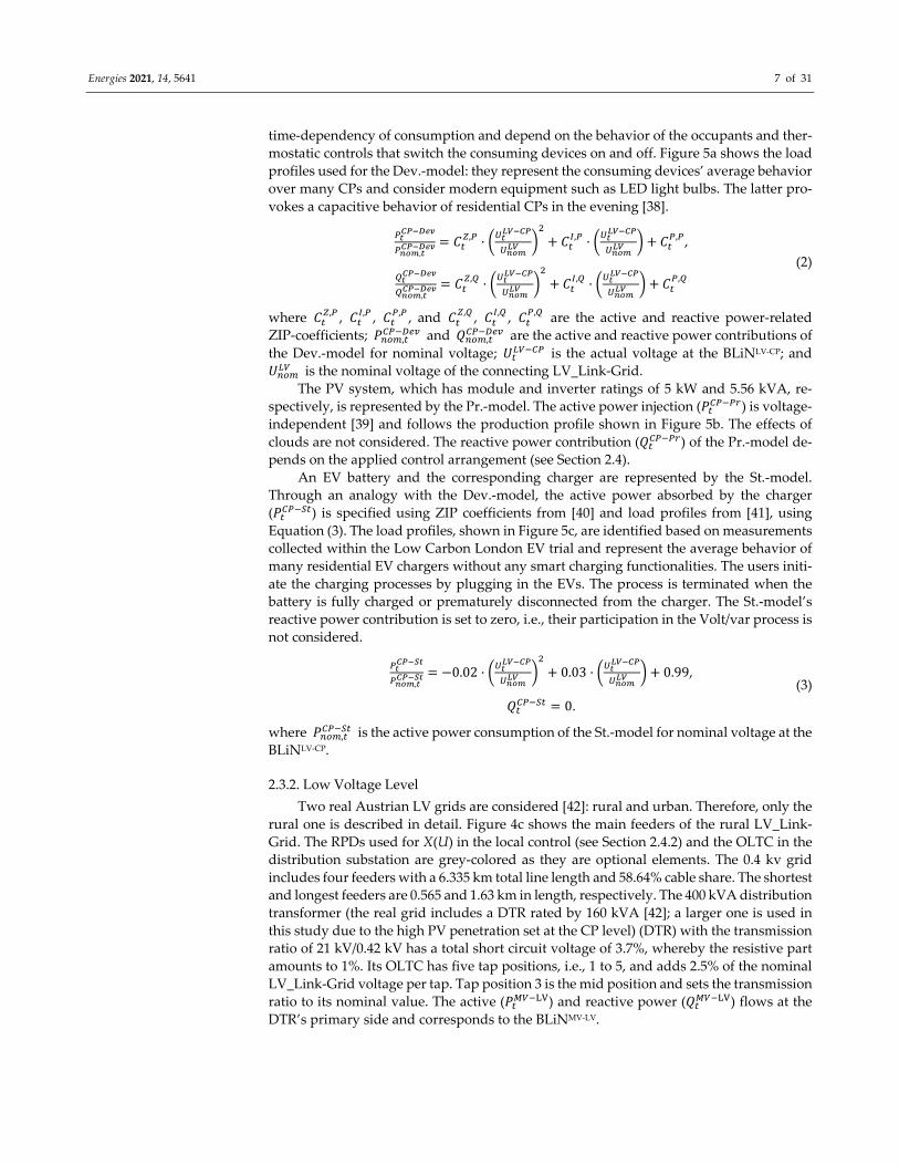
time‐dependency of consumption and depend on the behavior of the occupants and ther‐
mostatic controls that switch the consuming devices on and off. Figure 5a shows the load
profiles used for the Dev.‐model: they represent the consuming devices’ average behavior
over many CPs and consider modern equipment such as LED light bulbs. The latter pro‐
vokes a capacitive behavior of residential CPs in the evening [38].
,𝐶 , 𝐶 , 𝐶 , ,
,𝐶 , 𝐶 , 𝐶 ,
(2)
where 𝐶 , , 𝐶 , , 𝐶 , , and 𝐶 , , 𝐶 , , 𝐶 , are the active and reactive power‐related
ZIP‐coefficients; 𝑃 , and 𝑄 , are the active and reactive power contributions of
the Dev.‐model for nominal voltage; 𝑈 is the actual voltage at the BLiNLV‐CP; and
𝑈 is the nominal voltage of the connecting LV_Link‐Grid.
The PV system, which has module and inverter ratings of 5 kW and 5.56 kVA, re‐
spectively, is represented by the Pr.‐model. The active power injection (𝑃 ) is voltage‐
independent [39] and follows the production profile shown in Figure 5b. The effects of
clouds are not considered. The reactive power contribution (𝑄 ) of the Pr.‐model de‐
pends on the applied control arrangement (see Section 2.4).
An EV battery and the corresponding charger are represented by the St.‐model.
Through an analogy with the Dev.‐model, the active power absorbed by the charger
(𝑃 ) is specified using ZIP coefficients from [40] and load profiles from [41], using
Equation (3). The load profiles, shown in Figure 5c, are identified based on measurements
collected within the Low Carbon London EV trial and represent the average behavior of
many residential EV chargers without any smart charging functionalities. The users initi‐
ate the charging processes by plugging in the EVs. The process is terminated when the
battery is fully charged or prematurely disconnected from the charger. The St.‐model’s
reactive power contribution is set to zero, i.e., their participation in the Volt/var process is
not considered.
,0.02 0.03 0.99,
𝑄 0.
(3)
where 𝑃 , is the active power consumption of the St.‐model for nominal voltage at the
BLiNLV‐CP.
2.3.2. Low Voltage Level
Two real Austrian LV grids are considered [42]: rural and urban. Therefore, only the
rural one is described in detail. Figure 4c shows the main feeders of the rural LV_Link‐
Grid. The RPDs used for X(U) in the local control (see Section 2.4.2) and the OLTC in the
distribution substation are grey‐colored as they are optional elements. The 0.4 kv grid
includes four feeders with a 6.335 km total line length and 58.64% cable share. The shortest
and longest feeders are 0.565 and 1.63 km in length, respectively. The 400 kVA distribution
transformer (the real grid includes a DTR rated by 160 kVA [42]; a larger one is used in
this study due to the high PV penetration set at the CP level) (DTR) with the transmission
ratio of 21 kV/0.42 kV has a total short circuit voltage of 3.7%, whereby the resistive part
amounts to 1%. Its OLTC has five tap positions, i.e., 1 to 5, and adds 2.5% of the nominal
LV_Link‐Grid voltage per tap. Tap position 3 is the mid position and sets the transmission
ratio to its nominal value. The active (𝑃 ) and reactive power (𝑄 ) flows at the
DTR’s primary side and corresponds to the BLiNMV‐LV.
Energies 2021, 14, 5641 8 of 31
2.3.3. Medium Voltage Level
Figure 4d shows the main feeders of a real Austrian 20 kV MV_Link‐Grid. The STR
is not included in the model, and therefore BLiNHV‐MV corresponds to its secondary bus
bar. The active and reactive power flows at these boundaries are denoted as 𝑃 and
𝑄 , respectively. The six MV feeders have a total length and cable share of 267.151
km and 74.66%, respectively. The shortest and longest feeders have lengths of 2 and 46.10
km, respectively. Hydroelectric power plants, rated between 60 and 400 kW, are modeled
as PQ node‐elements that constantly inject 70% of their peak generation; they do not con‐
tribute any reactive power. Conforming to the German Grid Code [36], voltage limits of
0.9 and 1.1 p.u. are considered at their BPNs.
2.4. Description of Volt/var Control Arrangements
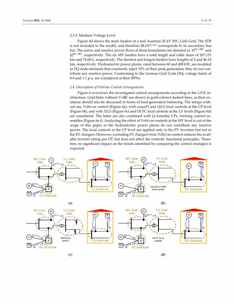
Figure 6 overviews the investigated control arrangements according to the LINK ar‐
chitecture. Grid‐links without VvSC are shown in gold‐colored dashed lines, as their ex‐
istence should also be discussed in terms of load‐generation balancing. The setups with‐
out any Volt/var control (Figure 6a), with cosφ(P) and Q(U) local controls at the CP level
(Figure 6b), and with X(U) (Figure 6c) and OLTC local controls at the LV levels (Figure 6d)
are considered. The latter are also combined with Q‐Autarkic CPs, forming control en‐
sembles (Figure 6e,f). Analyzing the effect of Volt/var controls at the MV level is out of the
scope of this paper as the hydroelectric power plants do not contribute any reactive
power. The local controls at the CP level are applied only to the PV inverters but not to
the EV chargers. However, excluding EV chargers from Volt/var control reduces the avail‐
able inverter rating per CP, but does not affect the controls’ functional principles. There‐
fore, no significant impact on the trends identified by comparing the control strategies is
expected.
(a) (b)
(c) (d)

Energies 2021, 14, 5641 9 of 31
(e) (f)
Figure 6. Overview of different Volt/var control arrangements: (a) no control; (b) cosφ(P) or Q(U) local control; (c) X(U)
local control; (d) OLTC local control; (e) X(U) local control and CP_Q‐Autarky; (f) OLTC local control and CP_Q‐Autarky.
2.4.1. No Volt/var Control
Figure 6a shows the chain setup without any Volt/var control. No VvSCs are in‐
volved, and all producers and storages inject or absorb active power with the unity power
factor. No RPDs and OLTCs are considered: the tap changers of all DTRs are fixed in mid‐
position.
2.4.2. Local Controls
Local controls are used to mitigate the voltage limit violations by avoiding the need
for any VvSCs.
cosφ(P) control at the CP level
Figure 6b shows the setup in which PV systems are upgraded with the cosφ(P)
local control. No RPDs and OLTCs are considered: the tap changers of all DTRs are
fixed in mid‐position. Equation (4) compactly presents the resulting Volt/var control
setup in the MV−LV−CP chain.
𝑉𝑣𝑪 𝑳𝑪 𝑐𝑜𝑠𝜑 𝑃 𝑜𝑟 𝑳𝑪 𝑄 𝑈 (4)
Figure 7a shows the cosφ(P) control characteristic specified by the Austrian Grid
Code [43] and used in all of the simulations. The inverters absorb reactive power
when their active power injection (𝑃 ) exceeds a certain value, which is com‐
monly set to 50% of the maximal active power production (𝑃 ). The inverters’
power factors (cos𝜑 ) are reduced from 1.0 down to 0.9 inductive in times of peak
production.
(a) (b)
Figure 7. Different control characteristics for PV inverters: (a) cosφ(P); (b) Q(U).
Q(U) local control at the CP level
Figure 6b and Equation (4) are also applied when PV systems are equipped with
the Q(U) local control. In this case, the PV inverters absorb the reactive power for high
local voltages and inject reactive power for low ones. Figure 7b shows the default Q(U)
Energies 2021, 14, 5641 10 of 31
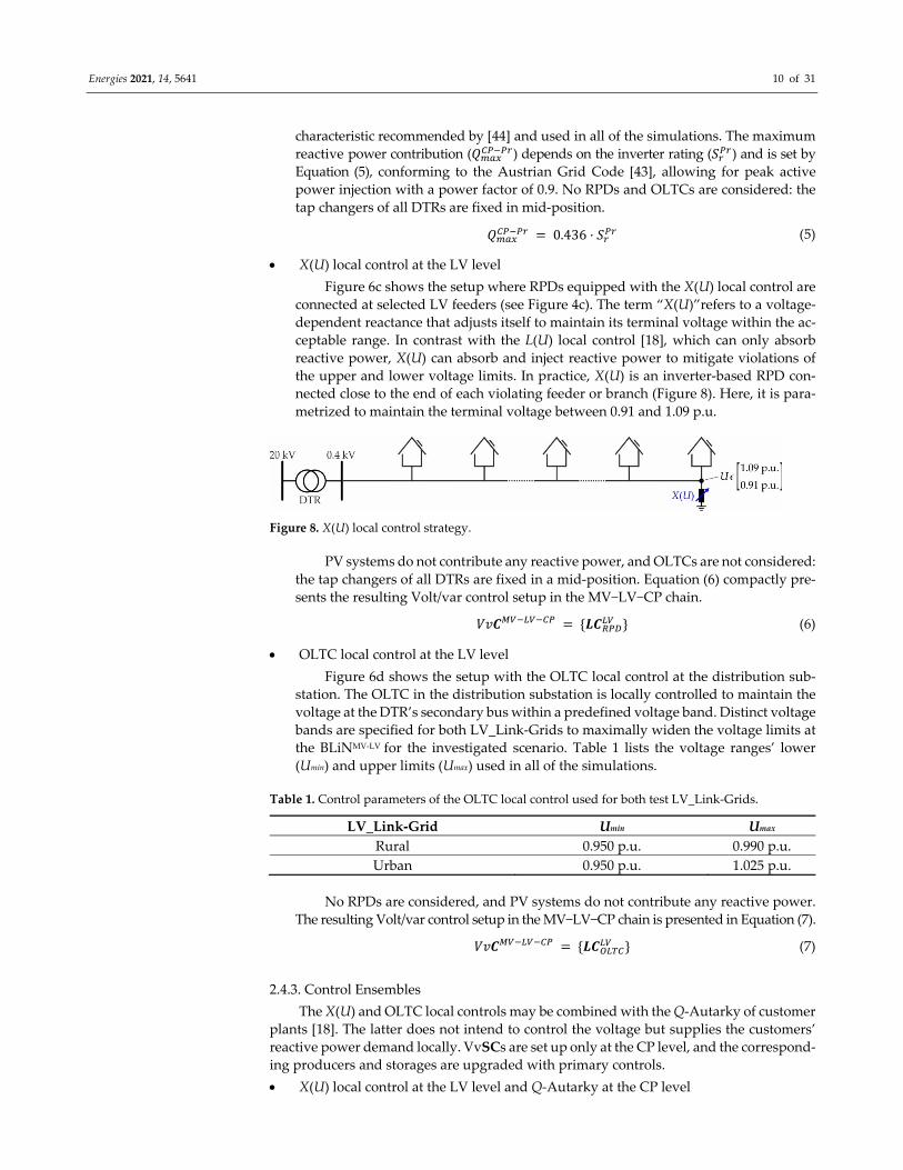
characteristic recommended by [44] and used in all of the simulations. The maximum
reactive power contribution (𝑄 ) depends on the inverter rating (𝑆 ) and is set by
Equation (5), conforming to the Austrian Grid Code [43], allowing for peak active
power injection with a power factor of 0.9. No RPDs and OLTCs are considered: the
tap changers of all DTRs are fixed in mid‐position.
𝑄 0.436 𝑆 (5)
X(U) local control at the LV level
Figure 6c shows the setup where RPDs equipped with the X(U) local control are
connected at selected LV feeders (see Figure 4c). The term “X(U)”refers to a voltage‐
dependent reactance that adjusts itself to maintain its terminal voltage within the ac‐
ceptable range. In contrast with the L(U) local control [18], which can only absorb
reactive power, X(U) can absorb and inject reactive power to mitigate violations of
the upper and lower voltage limits. In practice, X(U) is an inverter‐based RPD con‐
nected close to the end of each violating feeder or branch (Figure 8). Here, it is para‐
metrized to maintain the terminal voltage between 0.91 and 1.09 p.u.
Figure 8. X(U) local control strategy.
PV systems do not contribute any reactive power, and OLTCs are not considered:
the tap changers of all DTRs are fixed in a mid‐position. Equation (6) compactly pre‐
sents the resulting Volt/var control setup in the MV−LV−CP chain.
𝑉𝑣𝑪 𝑳𝑪 (6)
OLTC local control at the LV level
Figure 6d shows the setup with the OLTC local control at the distribution sub‐
station. The OLTC in the distribution substation is locally controlled to maintain the
voltage at the DTR’s secondary bus within a predefined voltage band. Distinct voltage
bands are specified for both LV_Link‐Grids to maximally widen the voltage limits at
the BLiNMV‐LV for the investigated scenario. Table 1 lists the voltage ranges’ lower
(Umin) and upper limits (Umax) used in all of the simulations.
Table 1. Control parameters of the OLTC local control used for both test LV_Link‐Grids.
LV_Link‐Grid Umin Umax
Rural 0.950 p.u. 0.990 p.u.
Urban 0.950 p.u. 1.025 p.u.
No RPDs are considered, and PV systems do not contribute any reactive power.
The resulting Volt/var control setup in the MV−LV−CP chain is presented in Equation (7).
𝑉𝑣𝑪 𝑳𝑪 (7)
2.4.3. Control Ensembles
The X(U) and OLTC local controls may be combined with the Q‐Autarky of customer
plants [18]. The latter does not intend to control the voltage but supplies the customers’
reactive power demand locally. VvSCs are set up only at the CP level, and the correspond‐
ing producers and storages are upgraded with primary controls.
X(U) local control at the LV level and Q‐Autarky at the CP level
Energies 2021, 14, 5641 11 of 31
Figure 6e shows the setup where the X(U) local control is combined with CP_Q‐
Autarky. To realize CP_Q‐Autarky, the 𝑉𝑣𝑺𝑪 adapts the primary control settings
of the corresponding producer‐ and storage‐Links to eliminate the reactive power
flow through the BLiNLV‐CP at all times. RPDs equipped with the X(U) local control
are connected at selected LV feeders (see Section 2.4.2). OLTCs are not considered: the
tap changers of all DTRs are fixed in mid‐position. Equation (8) compactly presents
the resulting Volt/var control setup.
𝑉𝑣𝑪 𝑳𝑪 ,𝑉𝑣𝑺𝑪 𝑷𝑪 ,𝑷𝑪 ;𝑪𝒏𝒔 0 kvar (8)
OLTC local control at the LV level and Q‐Autarky at the CP level
Figure 6f shows the setup where the OLTC local control is combined with Q‐
Autarkic CPs. The CPs do not exchange any reactive power with the LV and MV
grids. DTRs are upgraded with OLTC local controls (see Section 2.4.2), and no RPDs
are considered. The resulting Volt/var control setup is presented in Equation (9).
𝑉𝑣𝑪 𝑳𝑪 ,𝑉𝑣𝑺𝑪 𝑷𝑪 ,𝑷𝑪 ;𝑪𝒏𝒔 0 kvar (9)
3. Link‐Grid Behavior under Different Volt/var Control Arrangements
This section discusses the behavior of the test link chain at different system boundaries
by computing the load flows for the Volt/var control arrangements presented in Section 2.4.
Therefore, the P(U) and Q(U) behavior and the voltage limits are calculated at the MV−LV
and HV−MV boundaries. The grid losses, DTR loadings, and power flows over system
boundaries are discussed in detail for the cases listed in Table 2. The active power flows
are analyzed exclusively for the setup without any Volt/var control, because the different
control strategies only slightly modify it. Depending on the viewpoint, the boundary volt‐
age may apply to the HV−MV or MV−LV boundary node. The behavior at the MV−LV
boundary is discussed only for the rural LV_Link‐Grid, as the same trends are observed
in the urban one.
Table 2. Voltage−time‐pairs of the test cases discussed in detail.
Case Boundary Voltage Daytime
I 1.05 p.u. 06:00
II 0.95 p.u. 12:10
II 1.00 p.u. 12:10
III 1.00 p.u. 22:10
3.1. No Control
The voltage behavior, active and reactive power exchanges, active power losses, and
DTR loadings of the test link chain without any Volt/var control are discussed.
3.1.1. Voltage Behavior
Figure 9 shows the voltage limits at different boundaries of the test link chain. As
shown by the straight lines, the Grid Code fixes BVLLV‐CP, which correspond to the cus‐
tomer plants’ delivery points, at 0.9 and 1.1 p.u. Meanwhile, as the dashed and dotted
lines indicate, curved voltage limits (BVLMV‐LV and BVLHV‐MV) occur at the MV−LV and
HV−MV boundaries. Any violation of these limits results in violations of the legally stip‐
ulated voltage limits at the delivery points of CPs and hydropower plants.

Energies 2021, 14, 5641 12 of 31
Figure 9. Voltage limits at the LV−CP (rural residential CP_Link‐Grid), MV−LV (rural LV_Link‐
Grid), and HV−MV boundaries when no Volt/var control is applied.
The PV production strongly tightens the upper BVLMV‐LV and BVLHV‐MV, reaching very
low values of 0.9875 and 0.9175 p.u., respectively, at around noon‐time. Around midday,
limit violations occur for HV−MV and MV−LV boundary voltages of 0.95 (case II) and 1
p.u. (case II), respectively. The lower limits are tighten before 08:00 a.m. and after 16:15
p.m., i.e., when no significant PV injection is present. The lower BVLMV‐LV and BVLHV‐MV
reach 0.9525 and 1.0175 p.u., respectively, in the evening hours. The results clearly show
that the test link chain can hardly be operated without additional measures.
The LV feeders’ voltage profiles are shown in Figure 10a,b for cases II and II, respec‐
tively. The upper LV−CP boundary voltage limit at 12:10 p.m. (𝐵𝑉𝐿 : ) is indicated by a
dashed black line. While the boundary link nodes to the rural residential CP_Link‐Grids are
marked as black dots, the BLiNMV‐LV is highlighted as a grey cross. The PV injections consid‐
erably raise the feeder voltages, provoking upper limit violations in case II (Figure 10b).
(a) (b)
Figure 10. Voltage profiles of the rural LV_Link‐Grid’s feeders without any Volt/var control at 12:10 p.m. for different
MV−LV boundary voltages: (a) 0.95 p.u. (case II); (b) 1.00 p.u. (case II).
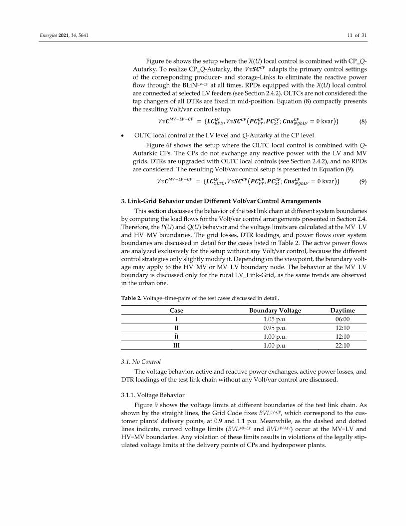
Figure 11 shows the MV feeders’ voltage profiles for case II. Black bullets and red
asterisks indicate the connection points of CP_Link‐Grids and hydroelectric power plants,
respectively. Meanwhile, connection points of urban and rural LV_Link‐Grids are high‐
lighted as violet and yellow asterisks, respectively.
Energies 2021, 14, 5641 13 of 31
Figure 11. MV feeders’ voltage profiles in case II.
Dashed lines in the same colors represent the upper BVLs. Conforming to the Grid
Code, an upper voltage limit of 𝐵𝑉𝐿 𝐵𝑉𝐿 1.1 p.u. prevails at the connec‐tion points of CP_Link‐Grids and power plants. At 12:10 p.m., maximal voltages of 1.0225
and 0.9875 p.u. are acceptable at the BLiNMV‐LV of the urban and rural LV_Link‐Grid, re‐
spectively (see Figure 9 for the rural one). The voltages increase up to 1.0161 p.u., provok‐
ing upper limit violations for some BLiNMV‐LV to the rural LV_Link‐Grid. Consequently,
case II lies within the upper limit violation zone. Figure 11 also shows that no LV_Link‐
Grids are connected to two relatively short MV feeders. This should be kept in mind when
comparing the different Volt/var control strategies: in contrast with the PV inverter‐based
controls, the X(U) and OLTC local controls do not affect the voltage profiles of these two
MV feeders.
3.1.2. Active Power Exchange
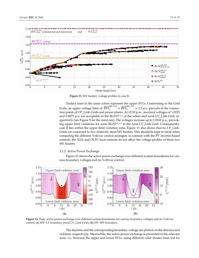
Figure 12 shows the active power exchange over different system boundaries for var‐
ious boundary voltages and no Volt/var control.
(a) (b)
Figure 12. Daily active power exchange over different system boundaries for various boundary voltages and no Volt/var
control: (a) MV−LV boundary (rural LV_Link‐Grid); (b) HV−MV boundary.
The daytime and the corresponding boundary voltage are plotted on the abscissa and
ordinate, respectively. Meanwhile, the active power exchange is presented in the relevant
zone, i.e., between the upper and lower BVLs, using different color shades from red for
Energies 2021, 14, 5641 14 of 31
the upstream flows (LV→MV and MV→HV) to violet for the downstream ones. The active
power flows through both regarded boundaries are characterized by an intense time‐ and
a weak voltage‐dependency. Flow direction changes twice a day.
From 00:00 a.m. to 08:00 a.m., the LV_Link‐Grid draws active power from the MV
level, consuming 56.62 kW in case I (Figure 12a). When the total PV production exceeds
the total consumption, i.e., from 08:00 a.m. to 16:15 p.m., the active power flow reverses,
reaching its maximum at 12:10 p.m. At this time, 241.99 kW is injected into the MV level
in case II. When consumption exceeds production, i.e., from 16:15 p.m. to 00:00 a.m., the
active power changes its direction again and flows from the MV into the LV_Link‐Grid.
In case III, the LV_Link‐Grid consumes 73.85 kW. Between 10:15 a.m. and 13:59 p.m., ac‐
tive power flows from the MV into the HV level, while before and afterwards, it flows in
reverse (Figure 12b). In cases I and III, 12.22 and 15.21 MW are absorbed by the MV_Link‐
Grid, respectively, while in case II, 6.22 MW flows into the HV level.
3.1.3. Reactive Power Exchange
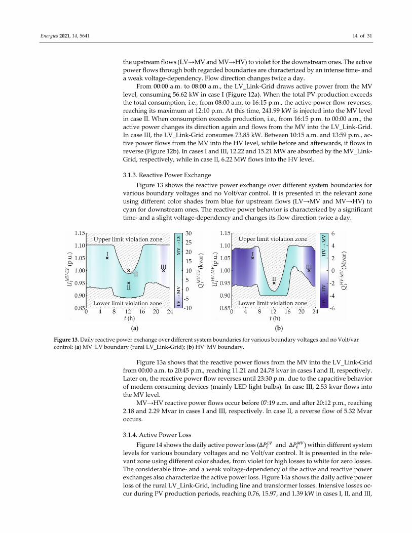
Figure 13 shows the reactive power exchange over different system boundaries for
various boundary voltages and no Volt/var control. It is presented in the relevant zone
using different color shades from blue for upstream flows (LV→MV and MV→HV) to
cyan for downstream ones. The reactive power behavior is characterized by a significant
time‐ and a slight voltage‐dependency and changes its flow direction twice a day.
(a) (b)
Figure 13. Daily reactive power exchange over different system boundaries for various boundary voltages and no Volt/var
control: (a) MV−LV boundary (rural LV_Link‐Grid); (b) HV−MV boundary.
Figure 13a shows that the reactive power flows from the MV into the LV_Link‐Grid
from 00:00 a.m. to 20:45 p.m., reaching 11.21 and 24.78 kvar in cases I and II, respectively.
Later on, the reactive power flow reverses until 23:30 p.m. due to the capacitive behavior
of modern consuming devices (mainly LED light bulbs). In case III, 2.53 kvar flows into
the MV level.
MV→HV reactive power flows occur before 07:19 a.m. and after 20:12 p.m., reaching
2.18 and 2.29 Mvar in cases I and III, respectively. In case II, a reverse flow of 5.32 Mvar
occurs.
3.1.4. Active Power Loss
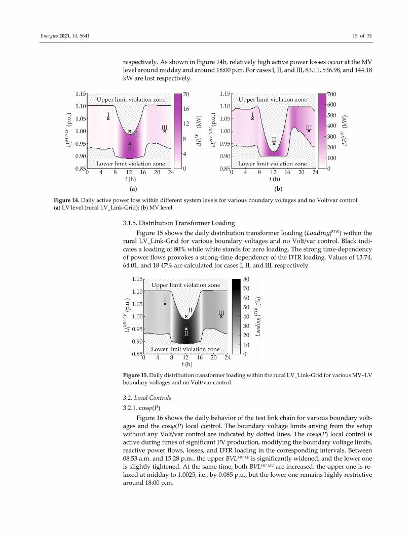
Figure 14 shows the daily active power loss (∆𝑃 and ∆𝑃 ) within different system
levels for various boundary voltages and no Volt/var control. It is presented in the rele‐
vant zone using different color shades, from violet for high losses to white for zero losses.
The considerable time‐ and a weak voltage‐dependency of the active and reactive power
exchanges also characterize the active power loss. Figure 14a shows the daily active power
loss of the rural LV_Link‐Grid, including line and transformer losses. Intensive losses oc‐
cur during PV production periods, reaching 0.76, 15.97, and 1.39 kW in cases I, II, and III,
Energies 2021, 14, 5641 15 of 31
respectively. As shown in Figure 14b, relatively high active power losses occur at the MV
level around midday and around 18:00 p.m. For cases I, II, and III, 83.11, 536.98, and 144.18
kW are lost respectively.
(a) (b)
Figure 14. Daily active power loss within different system levels for various boundary voltages and no Volt/var control:
(a) LV level (rural LV_Link‐Grid); (b) MV level.
3.1.5. Distribution Transformer Loading
Figure 15 shows the daily distribution transformer loading (𝐿𝑜𝑎𝑑𝑖𝑛𝑔 ) within the
rural LV_Link‐Grid for various boundary voltages and no Volt/var control. Black indi‐
cates a loading of 80% while white stands for zero loading. The strong time‐dependency
of power flows provokes a strong‐time dependency of the DTR loading. Values of 13.74,
64.01, and 18.47% are calculated for cases I, II, and III, respectively.
Figure 15. Daily distribution transformer loading within the rural LV_Link‐Grid for various MV−LV
boundary voltages and no Volt/var control.
3.2. Local Controls
3.2.1. cosφ(P)
Figure 16 shows the daily behavior of the test link chain for various boundary volt‐
ages and the cosφ(P) local control. The boundary voltage limits arising from the setup
without any Volt/var control are indicated by dotted lines. The cosφ(P) local control is
active during times of significant PV production, modifying the boundary voltage limits,
reactive power flows, losses, and DTR loading in the corresponding intervals. Between
08:53 a.m. and 15:28 p.m., the upper BVLMV‐LV is significantly widened, and the lower one
is slightly tightened. At the same time, both BVLHV‐MV are increased: the upper one is re‐
laxed at midday to 1.0025, i.e., by 0.085 p.u., but the lower one remains highly restrictive
around 18:00 p.m.
Energies 2021, 14, 5641 16 of 31
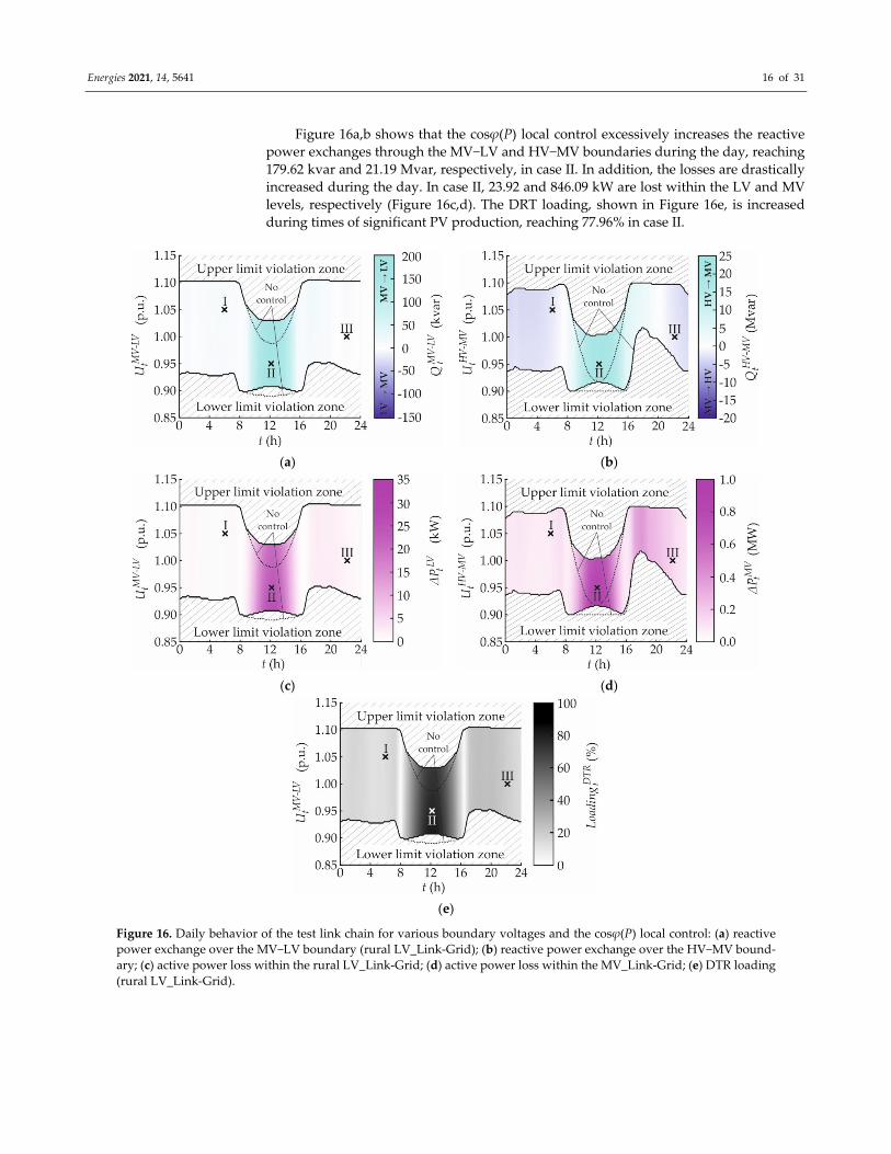
Figure 16a,b shows that the cosφ(P) local control excessively increases the reactive
power exchanges through the MV−LV and HV−MV boundaries during the day, reaching
179.62 kvar and 21.19 Mvar, respectively, in case II. In addition, the losses are drastically
increased during the day. In case II, 23.92 and 846.09 kW are lost within the LV and MV
levels, respectively (Figure 16c,d). The DRT loading, shown in Figure 16e, is increased
during times of significant PV production, reaching 77.96% in case II.
(a) (b)
(c) (d)
(e)
Figure 16. Daily behavior of the test link chain for various boundary voltages and the cosφ(P) local control: (a) reactive
power exchange over the MV−LV boundary (rural LV_Link‐Grid); (b) reactive power exchange over the HV−MV bound‐
ary; (c) active power loss within the rural LV_Link‐Grid; (d) active power loss within the MV_Link‐Grid; (e) DTR loading
(rural LV_Link‐Grid).
Energies 2021, 14, 5641 17 of 31
3.2.2. Q(U)
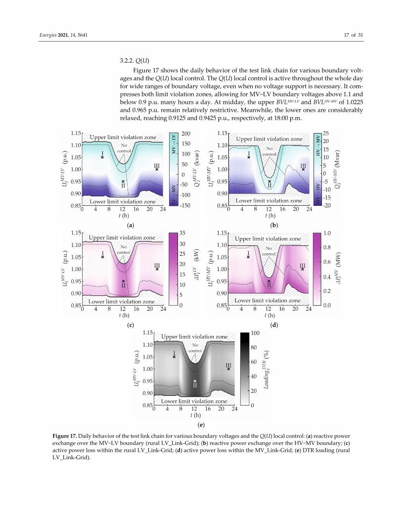
Figure 17 shows the daily behavior of the test link chain for various boundary volt‐
ages and the Q(U) local control. The Q(U) local control is active throughout the whole day
for wide ranges of boundary voltage, even when no voltage support is necessary. It com‐
presses both limit violation zones, allowing for MV−LV boundary voltages above 1.1 and
below 0.9 p.u. many hours a day. At midday, the upper BVLMV‐LV and BVLHV‐MV of 1.0225
and 0.965 p.u. remain relatively restrictive. Meanwhile, the lower ones are considerably
relaxed, reaching 0.9125 and 0.9425 p.u., respectively, at 18:00 p.m.
(a) (b)
(c) (d)
(e)
Figure 17. Daily behavior of the test link chain for various boundary voltages and the Q(U) local control: (a) reactive power
exchange over the MV−LV boundary (rural LV_Link‐Grid); (b) reactive power exchange over the HV−MV boundary; (c)
active power loss within the rural LV_Link‐Grid; (d) active power loss within the MV_Link‐Grid; (e) DTR loading (rural
LV_Link‐Grid).
Energies 2021, 14, 5641 18 of 31
The MV−LV reactive power exchange is considerably intensified in the edge regions
of the permissible voltage range (Figure 17a). Although no limit violations occur without
any Volt/var control, the reactive power exchange is increased to 26.02, 35.30, and −4.08
kvar in cases I, II, and III, respectively. The HV−MV reactive power exchange, shown in
Figure 17b, is modified almost in the complete voltage−time plane. In cases I and II, the
MV_Link‐Grid draws 0.11 and 6.40 Mvar from the HV level, respectively, while in case
III, it injects 2.59 Mvar. In addition, LV losses are increased in the edge regions of the
acceptable MV−LV boundary voltage range, provoking 0.83, 16.44, and 1.40 kW in cases
I, II, and III, respectively (Figure 17c). At the MV level, Q(U) increases the active power
loss for HV−MV boundary voltages close to the lower limit and decreases it for voltages
close to the upper limit (Figure 17d). Consequently, the loss is reduced to 52.61 kW in case
I and increased to 538.54 and 149.24 kW in cases II and III, respectively. The additional
reactive power flows provoked by Q(U) increase the DTR loading (Figure 17e). In cases I,
II, and III, the DTR is loaded by 14.82, 64.27, and 18.50%, respectively.
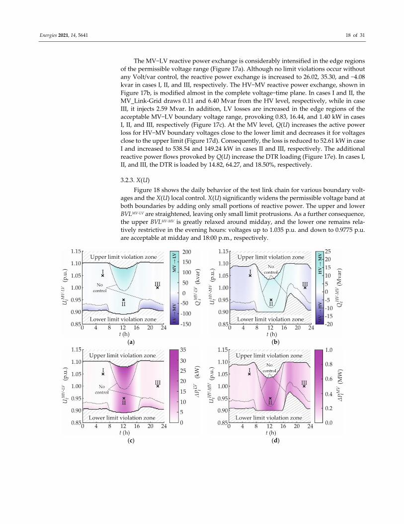
3.2.3. X(U)
Figure 18 shows the daily behavior of the test link chain for various boundary volt‐
ages and the X(U) local control. X(U) significantly widens the permissible voltage band at
both boundaries by adding only small portions of reactive power. The upper and lower
BVLMV‐LV are straightened, leaving only small limit protrusions. As a further consequence,
the upper BVLHV‐MV is greatly relaxed around midday, and the lower one remains rela‐
tively restrictive in the evening hours: voltages up to 1.035 p.u. and down to 0.9775 p.u.
are acceptable at midday and 18:00 p.m., respectively.
(a) (b)
(c) (d)
Energies 2021, 14, 5641 19 of 31
(e)
Figure 18. Daily behavior of the test link chain for various boundary voltages and the X(U) local control: (a) reactive power
exchange over the MV−LV boundary (rural LV_Link‐Grid); (b) reactive power exchange over the HV−MV boundary; (c)
active power loss within the rural LV_Link‐Grid; (d) active power loss within the MV_Link‐Grid; (e) DTR loading (rural
LV_Link‐Grid).
X(U) is active mainly in (U,t)‐regions where limit violations would occur without any
Volt/var control: it is inactive in the selected cases from the viewpoint of the BLiNMV‐LV
and active in case II from the perspective of the BLiNHV‐MV. Consequently, the MV−LV
reactive power exchanges (Figure 18a), LV active power loss (Figure 18c), and DTR load‐
ing (Figure 18d) are not affected in cases I, II, and III. Meanwhile, in case II, the reactive
power flow through the BLiNHV‐MV is increased to 5.52 Mvar (Figure 18b), modifying the
corresponding MV active power loss insignificantly (Figure 18d).
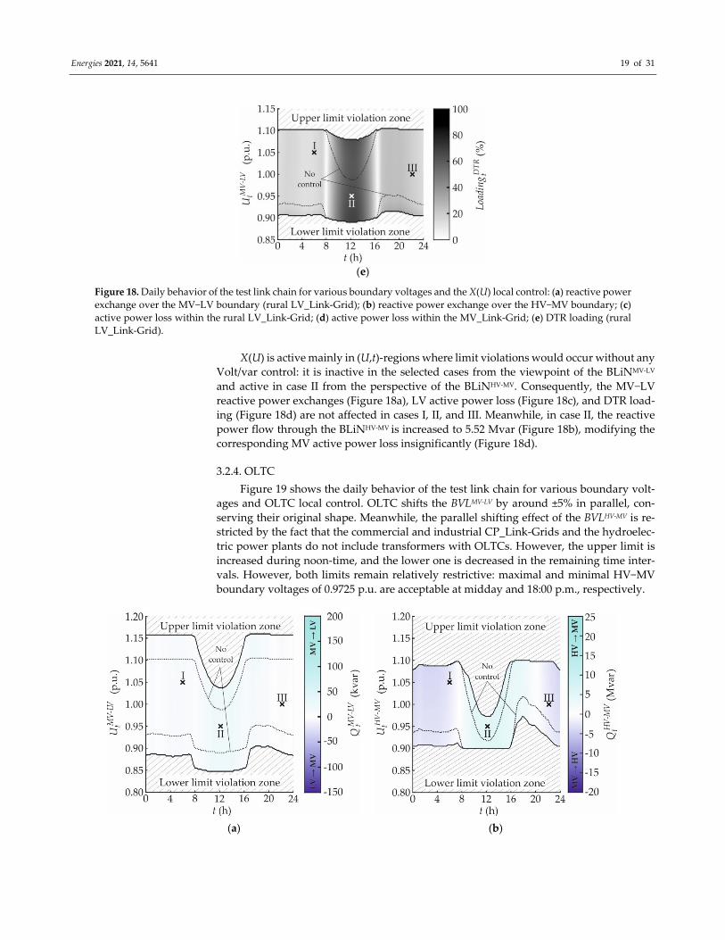
3.2.4. OLTC
Figure 19 shows the daily behavior of the test link chain for various boundary volt‐
ages and OLTC local control. OLTC shifts the BVLMV‐LV by around ±5% in parallel, con‐
serving their original shape. Meanwhile, the parallel shifting effect of the BVLHV‐MV is re‐
stricted by the fact that the commercial and industrial CP_Link‐Grids and the hydroelec‐
tric power plants do not include transformers with OLTCs. However, the upper limit is
increased during noon‐time, and the lower one is decreased in the remaining time inter‐
vals. However, both limits remain relatively restrictive: maximal and minimal HV−MV
boundary voltages of 0.9725 p.u. are acceptable at midday and 18:00 p.m., respectively.
(a) (b)
Energies 2021, 14, 5641 20 of 31
(c) (d)
(e)
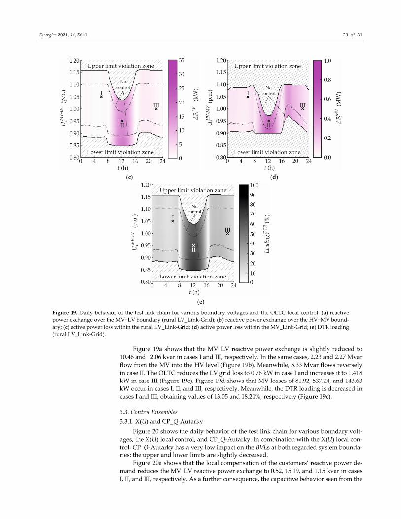
Figure 19. Daily behavior of the test link chain for various boundary voltages and the OLTC local control: (a) reactive
power exchange over the MV−LV boundary (rural LV_Link‐Grid); (b) reactive power exchange over the HV−MV bound‐
ary; (c) active power loss within the rural LV_Link‐Grid; (d) active power loss within the MV_Link‐Grid; (e) DTR loading
(rural LV_Link‐Grid).
Figure 19a shows that the MV−LV reactive power exchange is slightly reduced to
10.46 and −2.06 kvar in cases I and III, respectively. In the same cases, 2.23 and 2.27 Mvar
flow from the MV into the HV level (Figure 19b). Meanwhile, 5.33 Mvar flows reversely
in case II. The OLTC reduces the LV grid loss to 0.76 kW in case I and increases it to 1.418
kW in case III (Figure 19c). Figure 19d shows that MV losses of 81.92, 537.24, and 143.63
kW occur in cases I, II, and III, respectively. Meanwhile, the DTR loading is decreased in
cases I and III, obtaining values of 13.05 and 18.21%, respectively (Figure 19e).
3.3. Control Ensembles
3.3.1. X(U) and CP_Q‐Autarky
Figure 20 shows the daily behavior of the test link chain for various boundary volt‐
ages, the X(U) local control, and CP_Q‐Autarky. In combination with the X(U) local con‐
trol, CP_Q‐Autarky has a very low impact on the BVLs at both regarded system bounda‐
ries: the upper and lower limits are slightly decreased.
Figure 20a shows that the local compensation of the customers’ reactive power de‐
mand reduces the MV−LV reactive power exchange to 0.52, 15.19, and 1.15 kvar in cases
I, II, and III, respectively. As a further consequence, the capacitive behavior seen from the

Energies 2021, 14, 5641 21 of 31
HV level is intensified in cases I and III, reaching 7.48 and 6.58 Mvar, respectively (Figure
20b). In case II, the reactive power flow is reversed: 4.75 Mvar flow into the HV level. The
reduced reactive power flows at the LV level reduce the corresponding losses to 0.74,
15.86, and 1.39 kW in cases I, II, and III, respectively (Figure 20c). Meanwhile, Figure 20d
shows that the MV losses are increased to 121.45, 554.80, and 181.14 kW, respectively. The
DTR is slightly unloaded by the Q‐Autarky of CPs, reaching 13.51, 63.81, and 18.46% in
cases I, II, and III, respectively (Figure 20e).
3.3.2. OLTC and CP_Q‐Autarky
Figure 21 shows the daily behavior of the test link chain for various boundary volt‐
ages, the OLTC local control, and CP_Q‐Autarky. In addition, combined with OLTC local
control, Q‐Autarky of CPs slightly reduces the upper and lower BVLs at both boundaries.
As shown in Figure 21a, this control ensemble greatly reduces the MV−LV reactive
power exchange to 0.54, 15.19, and 1.18 kvar in cases I, II, and III, respectively. Figure 21b
shows that the MV grid is capacitive in the complete voltage−time plane, injecting 7.48,
5.14, and 6.58 Mvar into the HV level in cases I, II, and III, respectively. The reduced Q‐
flows at the LV level decrease the corresponding losses to 0.74, 15.86, and 1.416 kW for
cases I, II, and III, respectively (Figure 21c). Meanwhile, according to Figure 21d, MV
losses are increased to 119.65, 572.32, and 180.34 kWm, respectively. Due to the reduced
reactive power flows through the DTR, its loading is decreased to 12.84, 63.81, and 18.20%
in cases I, II, and III, respectively (Figure 21e).
(a) (b)
(c) (d)

Energies 2021, 14, 5641 22 of 31
(e)
Figure 20. Daily behavior of the test link chain for various boundary voltages, the X(U) local control, and CP_Q‐Autarky:
(a) reactive power exchange over the MV−LV boundary (rural LV_Link‐Grid); (b) reactive power exchange over the
HV−MV boundary; (c) active power loss within the rural LV_Link‐Grid; (d) active power loss within the MV_Link‐Grid;
(e) DTR loading (rural LV_Link‐Grid).
(a) (b)
(c) (d)
Energies 2021, 14, 5641 23 of 31
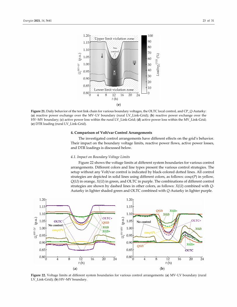
(e)
Figure 21. Daily behavior of the test link chain for various boundary voltages, the OLTC local control, and CP_Q‐Autarky:
(a) reactive power exchange over the MV−LV boundary (rural LV_Link‐Grid); (b) reactive power exchange over the
HV−MV boundary; (c) active power loss within the rural LV_Link‐Grid; (d) active power loss within the MV_Link‐Grid;
(e) DTR loading (rural LV_Link‐Grid).
4. Comparison of Volt/var Control Arrangements
The investigated control arrangements have different effects on the grid’s behavior.
Their impact on the boundary voltage limits, reactive power flows, active power losses,
and DTR loadings is discussed below.
4.1. Impact on Boundary Voltage Limits
Figure 22 shows the voltage limits at different system boundaries for various control
arrangements. Different colors and line types present the various control strategies. The
setup without any Volt/var control is indicated by black‐colored dotted lines. All control
strategies are depicted in solid lines using different colors, as follows: cosφ(P) in yellow,
Q(U) in orange, X(U) in green, and OLTC in purple. The combinations of different control
strategies are shown by dashed lines in other colors, as follows: X(U) combined with Q‐
Autarky in lighter shaded green and OLTC combined with Q‐Autarky in lighter purple.
(a) (b)
Figure 22. Voltage limits at different system boundaries for various control arrangements: (a) MV−LV boundary (rural
LV_Link‐Grid); (b) HV−MV boundary.
Energies 2021, 14, 5641 24 of 31
Whether combined with CP_Q‐Autarky or not, the X(U) local control has the greatest
impact on the upper BVLMV‐LV around midday (Figure 22a): it allows for MV−LV boundary
voltages up to 1.08 p.u. In contrast, using cosφ(P), Q(U), or OLTC local controls severely
restricts the upper voltage limit to be respected at the distribution substation. Regarding
the lower BVLMV‐LV, OLTC shows the best results: the limit remains below 0.905 p.u.
throughout the whole day, reaching its maximum value in the early evening hours. In
addition, at the BLiNHV‐MV, the X(U) local control has the most significant impact on the
upper BVL at noon‐time (Figure 22b). The other local controls provoke highly restrictive
upper voltage limits to be respected at the supplying substation. Meanwhile, the Q(U)
local control decreases the lower BVLHV‐MV the best, and cosφ(P) yields unacceptable re‐
strictive limits.
In any case, the BVLs are significantly deformed compared with the constant voltage
limits stipulated by the Grid Code. The concept of voltage limit distortion (VLD) is intro‐
duced to evaluate the impact of different control strategies on the time‐variability of
boundary voltage limits. It is calculated by Equation (10). The larger the VLD, the more
actions are required during the day to maintain the voltage.
𝑉𝐿𝐷 𝑉𝐿𝐷 𝑉𝐿𝐷 (10)
where c indexes the control arrangement for which the VLD is calculated; 𝑡 is the time
interval n; 𝑁 1 is the number of simulated time intervals; and 𝐵𝑉𝐿 , 𝐵𝑉𝐿 ,
𝐵𝑉𝐿 , and 𝐵𝑉𝐿 are the upper and lower MV−LV and HV−MV boundary volt‐
age limits, respectively.
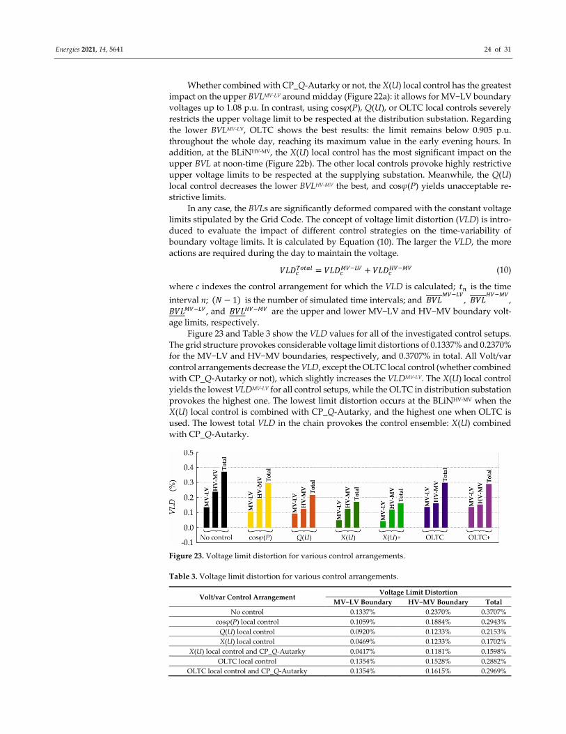
Figure 23 and Table 3 show the VLD values for all of the investigated control setups.
The grid structure provokes considerable voltage limit distortions of 0.1337% and 0.2370%
for the MV−LV and HV−MV boundaries, respectively, and 0.3707% in total. All Volt/var
control arrangements decrease the VLD, except the OLTC local control (whether combined
with CP_Q‐Autarky or not), which slightly increases the VLDMV‐LV. The X(U) local control
yields the lowest VLDMV‐LV for all control setups, while the OLTC in distribution substation
provokes the highest one. The lowest limit distortion occurs at the BLiNHV‐MV when the
X(U) local control is combined with CP_Q‐Autarky, and the highest one when OLTC is
used. The lowest total VLD in the chain provokes the control ensemble: X(U) combined
with CP_Q‐Autarky.
Figure 23. Voltage limit distortion for various control arrangements.
Table 3. Voltage limit distortion for various control arrangements.
Volt/var Control Arrangement Voltage Limit Distortion
MV−LV Boundary HV−MV Boundary Total
No control 0.1337% 0.2370% 0.3707%
cosφ(P) local control 0.1059% 0.1884% 0.2943%
Q(U) local control 0.0920% 0.1233% 0.2153%
X(U) local control 0.0469% 0.1233% 0.1702%
X(U) local control and CP_Q‐Autarky 0.0417% 0.1181% 0.1598%
OLTC local control 0.1354% 0.1528% 0.2882%
OLTC local control and CP_Q‐Autarky 0.1354% 0.1615% 0.2969%

Energies 2021, 14, 5641 25 of 31
4.2. Impact on Reactive Power Flows
Figure 24 shows the composition of the reactive power exchanged for different control
strategies and cases. The reactive power crossing the MV−LV boundary, shown in Figure 24a,
consists of two components: the Q‐amount of CP_Link‐Grids, which is determined by the
corresponding consuming devices and PV systems, and the Q‐amount of the LV_Link‐
Grid itself, which represents the reactive power contributions of the LV lines, DTR, and
RPDs (only relevant when the X(U) local control is used). Significant Q‐amounts of the
LV_Link‐Grid are found only in case II, where relatively high reactive power losses occur.
The cosφ(P) local control drastically increases the CPs’ reactive power consumptions in
case II, causing additional reactive power losses as a further consequence. Q(U) intensifies
the LV−CP reactive power exchanges in all cases. Due to its inactivity in the selected cases,
the X(U) local control does not modify the corresponding reactive power compositions.
In cases I and III, the OLTC reduces the CPs’ Q‐amounts while increasing the reactive
power losses at the LV level. With both control ensembles, Q‐Autarkic customers do not
exchange any reactive power with the grid, reducing the grid’s reactive power loss.
(a)
(b)
Figure 24. Composition of the reactive power exchange for various control strategies and cases in
different system boundaries: (a) MV−LV; (b) HV−MV.
The MV_Link‐Grid connects CP and LV_Link‐Grids and hydroelectric power plants.
Therefore, the reactive power flow through the BLiNHV‐MV, shown in Figure 24b, contains
Q‐amounts of three different components: commercial and industrial CP_Link‐Grids, ur‐
ban and rural LV_Link‐Grids, and the MV_Link‐Grid itself. The hydroelectric power
plants do not contribute any reactive power. Due to its high cable share, the MV_Link‐
Grid generally produces significant amounts of reactive power. Especially in case II, this
reactive power production is partly compensated by the reactive power losses in the MV
lines’ series impedances. Non‐Q‐Autarkic CPs consume substantial amounts of reactive
power for all of the control arrangements. This Q‐consumption is significantly intensified
by the cosφ(P) local control in case II and by Q(U) in case I. Furthermore, the Q(U) and
especially cosφ(P) local controls considerably increase the reactive power consumption of
LV_Link‐Grids, as they enlarge the Q‐consumption of the thereto connected residential
Energies 2021, 14, 5641 26 of 31
CPs. Meanwhile, the X(U) and OLTC local controls have low impacts on the Q‐composi‐
tion at the BLiNHV‐MV. In any combination, CP_Q‐Autarky eliminates the reactive power
contributions of CPs and reduces the ones of the LV_Link‐Grids.
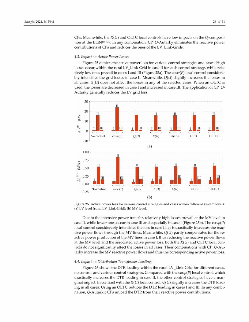
4.3. Impact on Active Power Losses
Figure 25 depicts the active power loss for various control strategies and cases. High
losses occur within the rural LV_Link‐Grid in case II for each control strategy, while rela‐
tively low ones prevail in cases I and III (Figure 25a). The cosφ(P) local control considera‐
bly intensifies the grid losses in case II. Meanwhile, Q(U) slightly increases the losses in
all cases. X(U) does not affect the losses in any of the selected cases. When an OLTC is
used, the losses are decreased in case I and increased in case III. The application of CP_Q‐
Autarky generally reduces the LV grid loss.
(a)
(b)
Figure 25. Active power loss for various control strategies and cases within different system levels:
(a) LV level (rural LV_Link‐Grid); (b) MV level.
Due to the intensive power transfer, relatively high losses prevail at the MV level in
case II, while lower ones occur in case III and especially in case I (Figure 25b). The cosφ(P)
local control considerably intensifies the loss in case II, as it drastically increases the reac‐
tive power flows through the MV lines. Meanwhile, Q(U) partly compensates for the re‐
active power production of the MV lines in case I, thus reducing the reactive power flows
at the MV level and the associated active power loss. Both the X(U) and OLTC local con‐
trols do not significantly affect the losses in all cases. Their combinations with CP_Q‐Au‐
tarky increase the MV reactive power flows and thus the corresponding active power loss.
4.4. Impact on Distribution Transformer Loadings
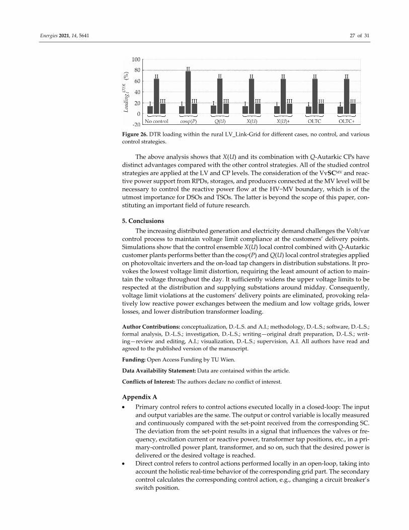
Figure 26 shows the DTR loading within the rural LV_Link‐Grid for different cases,
no control, and various control strategies. Compared with the cosφ(P) local control, which
drastically increases the DTR loading in case II, the other control strategies have a mar‐
ginal impact. In contrast with the X(U) local control, Q(U) slightly increases the DTR load‐
ing in all cases. Using an OLTC reduces the DTR loading in cases I and III. In any combi‐
nation, Q‐Autarkic CPs unload the DTR from their reactive power contributions.
Energies 2021, 14, 5641 27 of 31
Figure 26. DTR loading within the rural LV_Link‐Grid for different cases, no control, and various
control strategies.
The above analysis shows that X(U) and its combination with Q‐Autarkic CPs have
distinct advantages compared with the other control strategies. All of the studied control
strategies are applied at the LV and CP levels. The consideration of the VvSCMV and reac‐
tive power support from RPDs, storages, and producers connected at the MV level will be
necessary to control the reactive power flow at the HV−MV boundary, which is of the
utmost importance for DSOs and TSOs. The latter is beyond the scope of this paper, con‐
stituting an important field of future research.
5. Conclusions
The increasing distributed generation and electricity demand challenges the Volt/var
control process to maintain voltage limit compliance at the customers’ delivery points.
Simulations show that the control ensemble X(U) local control combined with Q‐Autarkic
customer plants performs better than the cosφ(P) and Q(U) local control strategies applied
on photovoltaic inverters and the on‐load tap changers in distribution substations. It pro‐
vokes the lowest voltage limit distortion, requiring the least amount of action to main‐
tain the voltage throughout the day. It sufficiently widens the upper voltage limits to be
respected at the distribution and supplying substations around midday. Consequently,
voltage limit violations at the customers’ delivery points are eliminated, provoking rela‐
tively low reactive power exchanges between the medium and low voltage grids, lower
losses, and lower distribution transformer loading.
Author Contributions: conceptualization, D.‐L.S. and A.I.; methodology, D.‐L.S.; software, D.‐L.S.;
formal analysis, D.‐L.S.; investigation, D.‐L.S.; writing—original draft preparation, D.‐L.S.; writ‐
ing—review and editing, A.I.; visualization, D.‐L.S.; supervision, A.I. All authors have read and
agreed to the published version of the manuscript.
Funding: Open Access Funding by TU Wien.
Data Availability Statement: Data are contained within the article.
Conflicts of Interest: The authors declare no conflict of interest.
Appendix A
Primary control refers to control actions executed locally in a closed‐loop: The input
and output variables are the same. The output or control variable is locally measured
and continuously compared with the set‐point received from the corresponding SC.
The deviation from the set‐point results in a signal that influences the valves or fre‐
quency, excitation current or reactive power, transformer tap positions, etc., in a pri‐
mary‐controlled power plant, transformer, and so on, such that the desired power is
delivered or the desired voltage is reached.
Direct control refers to control actions performed locally in an open‐loop, taking into
account the holistic real‐time behavior of the corresponding grid part. The secondary
control calculates the corresponding control action, e.g., changing a circuit breaker’s
switch position.
Energies 2021, 14, 5641 28 of 31
Secondary control refers to control variables that are calculated based on the current
state of a control area. It fulfills a predefined objective function by respecting static
and dynamic constraints (P/Q capabilities of generators, transformer and line rating,
voltage limits, reactive power limits, etc.). It calculates and sends the set‐points to
PCs and the input variables DiCs acting on its area.
Local control refers to control actions that are carried out locally without considering
the holistic real‐time behavior of the relevant grid part. Its action path may be real‐
ized in an open‐ or closed‐loop. LC automatically adjusts the active/reactive power
contributions of RPDs, storages, and producers and the tap positions of transformers
based on local measurements or time schedules [21,45,46]. It usually maintains a
power system parameter, which is locally measured or calculated based on local
measurements, equal to the desired value. The fixed control settings are calculated
based on offline system analysis for typical operating conditions. LCs are simple, re‐
liable, and respond quickly to changing operating conditions without the need for a
communication infrastructure [47–49].
Appendix B
The models of the urban residential, commercial, and industrial CP_Link‐Grids are
presented below.
Urban residential CP_Link‐Grid
This CP type is connected to the urban LV_Link‐Grid. It has the same structure
and profiles as the rural residential one (see Figure 5a), except for one detail: the Dev.‐
model’s load profiles are increased by the factor 1.43.
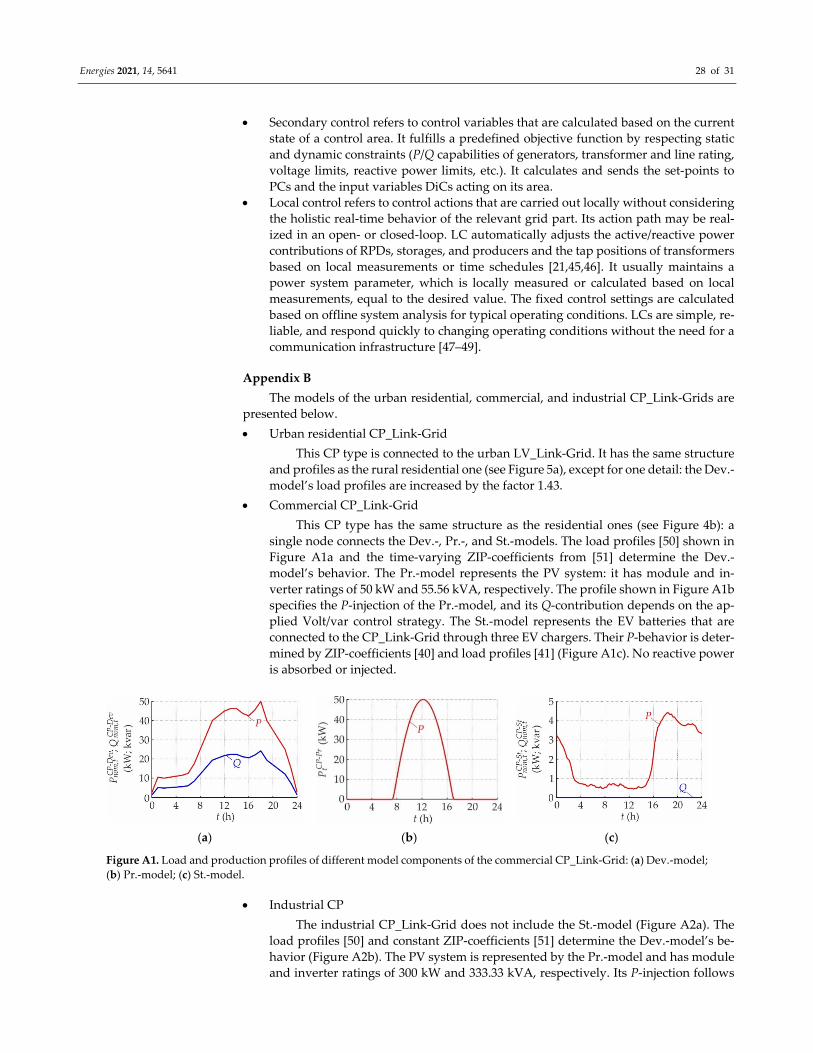
Commercial CP_Link‐Grid
This CP type has the same structure as the residential ones (see Figure 4b): a
single node connects the Dev.‐, Pr.‐, and St.‐models. The load profiles [50] shown in
Figure A1a and the time‐varying ZIP‐coefficients from [51] determine the Dev.‐
model’s behavior. The Pr.‐model represents the PV system: it has module and in‐
verter ratings of 50 kW and 55.56 kVA, respectively. The profile shown in Figure A1b
specifies the P‐injection of the Pr.‐model, and its Q‐contribution depends on the ap‐
plied Volt/var control strategy. The St.‐model represents the EV batteries that are
connected to the CP_Link‐Grid through three EV chargers. Their P‐behavior is deter‐
mined by ZIP‐coefficients [40] and load profiles [41] (Figure A1c). No reactive power
is absorbed or injected.
(a) (b) (c)
Figure A1. Load and production profiles of different model components of the commercial CP_Link‐Grid: (a) Dev.‐model;
(b) Pr.‐model; (c) St.‐model.
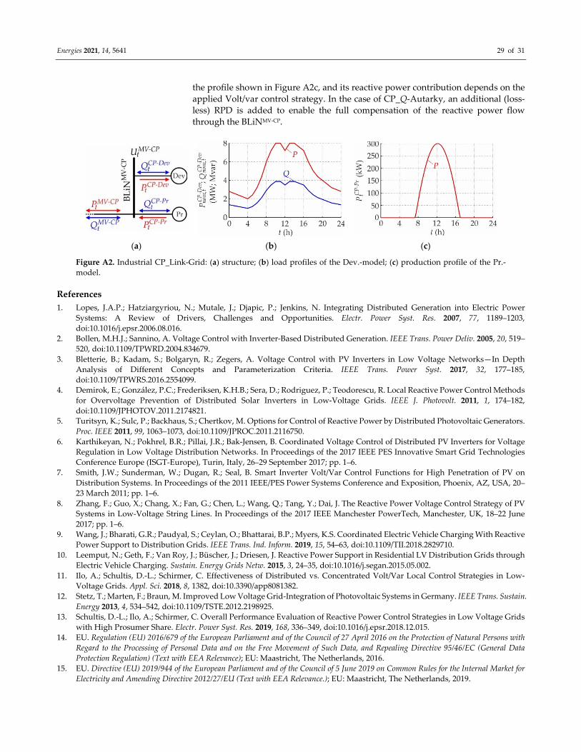
Industrial CP
The industrial CP_Link‐Grid does not include the St.‐model (Figure A2a). The
load profiles [50] and constant ZIP‐coefficients [51] determine the Dev.‐model’s be‐
havior (Figure A2b). The PV system is represented by the Pr.‐model and has module
and inverter ratings of 300 kW and 333.33 kVA, respectively. Its P‐injection follows
Energies 2021, 14, 5641 29 of 31
the profile shown in Figure A2c, and its reactive power contribution depends on the
applied Volt/var control strategy. In the case of CP_Q‐Autarky, an additional (loss‐
less) RPD is added to enable the full compensation of the reactive power flow
through the BLiNMV‐CP.
(a) (b) (c)
Figure A2. Industrial CP_Link‐Grid: (a) structure; (b) load profiles of the Dev.‐model; (c) production profile of the Pr.‐
model.
References
1. Lopes, J.A.P.; Hatziargyriou, N.; Mutale, J.; Djapic, P.; Jenkins, N. Integrating Distributed Generation into Electric Power
Systems: A Review of Drivers, Challenges and Opportunities. Electr. Power Syst. Res. 2007, 77, 1189–1203,
doi:10.1016/j.epsr.2006.08.016.
2. Bollen, M.H.J.; Sannino, A. Voltage Control with Inverter‐Based Distributed Generation. IEEE Trans. Power Deliv. 2005, 20, 519–
520, doi:10.1109/TPWRD.2004.834679.
3. Bletterie, B.; Kadam, S.; Bolgaryn, R.; Zegers, A. Voltage Control with PV Inverters in Low Voltage Networks—In Depth
Analysis of Different Concepts and Parameterization Criteria. IEEE Trans. Power Syst. 2017, 32, 177–185,
doi:10.1109/TPWRS.2016.2554099.
4. Demirok, E.; González, P.C.; Frederiksen, K.H.B.; Sera, D.; Rodriguez, P.; Teodorescu, R. Local Reactive Power Control Methods
for Overvoltage Prevention of Distributed Solar Inverters in Low‐Voltage Grids. IEEE J. Photovolt. 2011, 1, 174–182,
doi:10.1109/JPHOTOV.2011.2174821.
5. Turitsyn, K.; Sulc, P.; Backhaus, S.; Chertkov, M. Options for Control of Reactive Power by Distributed Photovoltaic Generators.
Proc. IEEE 2011, 99, 1063–1073, doi:10.1109/JPROC.2011.2116750.
6. Karthikeyan, N.; Pokhrel, B.R.; Pillai, J.R.; Bak‐Jensen, B. Coordinated Voltage Control of Distributed PV Inverters for Voltage
Regulation in Low Voltage Distribution Networks. In Proceedings of the 2017 IEEE PES Innovative Smart Grid Technologies
Conference Europe (ISGT‐Europe), Turin, Italy, 26–29 September 2017; pp. 1–6.
7. Smith, J.W.; Sunderman, W.; Dugan, R.; Seal, B. Smart Inverter Volt/Var Control Functions for High Penetration of PV on
Distribution Systems. In Proceedings of the 2011 IEEE/PES Power Systems Conference and Exposition, Phoenix, AZ, USA, 20–
23 March 2011; pp. 1–6.
8. Zhang, F.; Guo, X.; Chang, X.; Fan, G.; Chen, L.; Wang, Q.; Tang, Y.; Dai, J. The Reactive Power Voltage Control Strategy of PV
Systems in Low‐Voltage String Lines. In Proceedings of the 2017 IEEE Manchester PowerTech, Manchester, UK, 18–22 June
2017; pp. 1–6.
9. Wang, J.; Bharati, G.R.; Paudyal, S.; Ceylan, O.; Bhattarai, B.P.; Myers, K.S. Coordinated Electric Vehicle Charging With Reactive
Power Support to Distribution Grids. IEEE Trans. Ind. Inform. 2019, 15, 54–63, doi:10.1109/TII.2018.2829710.
10. Leemput, N.; Geth, F.; Van Roy, J.; Büscher, J.; Driesen, J. Reactive Power Support in Residential LV Distribution Grids through
Electric Vehicle Charging. Sustain. Energy Grids Netw. 2015, 3, 24–35, doi:10.1016/j.segan.2015.05.002.
11. Ilo, A.; Schultis, D.‐L.; Schirmer, C. Effectiveness of Distributed vs. Concentrated Volt/Var Local Control Strategies in Low‐
Voltage Grids. Appl. Sci. 2018, 8, 1382, doi:10.3390/app8081382.
12. Stetz, T.; Marten, F.; Braun, M. Improved Low Voltage Grid‐Integration of Photovoltaic Systems in Germany. IEEE Trans. Sustain.
Energy 2013, 4, 534–542, doi:10.1109/TSTE.2012.2198925.
13. Schultis, D.‐L.; Ilo, A.; Schirmer, C. Overall Performance Evaluation of Reactive Power Control Strategies in Low Voltage Grids
with High Prosumer Share. Electr. Power Syst. Res. 2019, 168, 336–349, doi:10.1016/j.epsr.2018.12.015.
14. EU. Regulation (EU) 2016/679 of the European Parliament and of the Council of 27 April 2016 on the Protection of Natural Persons with
Regard to the Processing of Personal Data and on the Free Movement of Such Data, and Repealing Directive 95/46/EC (General Data
Protection Regulation) (Text with EEA Relevance); EU: Maastricht, The Netherlands, 2016.
15. EU. Directive (EU) 2019/944 of the European Parliament and of the Council of 5 June 2019 on Common Rules for the Internal Market for
Electricity and Amending Directive 2012/27/EU (Text with EEA Relevance.); EU: Maastricht, The Netherlands, 2019.

Energies 2021, 14, 5641 30 of 31
16. Reese, C.; Buchhagen, C.; Hofmann, L. Voltage Range as Control Input for OLTC‐Equipped Distribution Transformers. In
Proceedings of the PES T&D 2012, Orlando, FL, USA, 7–10 May 2012; pp. 1–6.
17. Hossain, M.I.; Yan, R.; Saha, T. Investigation of the Interaction between Step Voltage Regulators and Large‐Scale Photovoltaic
Systems Regarding Voltage Regulation and Unbalance. IET Renew. Power Gener. 2016, 10, 299–309, doi:10.1049/IET‐
RPG.2015.0086.
18. Ilo, A.; Schultis, D.‐L. Low‐Voltage Grid Behaviour in the Presence of Concentrated Var‐Sinks and Var‐Compensated Customers.
Electr. Power Syst. Res. 2019, 171, 54–65, doi:10.1016/j.epsr.2019.01.031.
19. Ostergaard, J.; Ziras, C.; Bindner, H.W.; Kazempour, J.; Marinelli, M.; Markussen, P.; Rosted, S.H.; Christensen, J.S. Energy
Security Through Demand‐Side Flexibility: The Case of Denmark. IEEE Power Energy Mag. 2021, 19, 46–55,
doi:10.1109/MPE.2020.3043615.
20. Chiang, H.‐D.; Wang, J.‐C.; Tong, J.; Darling, G. Optimal Capacitor Placement, Replacement and Control in Large‐Scale
Unbalanced Distribution Systems: Modeling and a New Formulation. IEEE Trans. Power Syst. 1995, 10, 356–362,
doi:10.1109/59.373956.
21. Guo, Q.; Qi, J.; Ajjarapu, V.; Bravo, R.; Chow, J.; Li, Z.; Moghe, R.; Nasr‐Azadani, E.; Tamrakar, U.; Taranto, G.N.; et al. Review
of Challenges and Research Opportunities for Voltage Control in Smart Grids. IEEE Trans. Power Syst. 2019, 34, 2790–2801,
doi:10.1109/TPWRS.2019.2897948.
22. Lund, P. The Danish Cell Project—Part 1: Background and General Approach. In Proceedings of the 2007 IEEE Power
Engineering Society General Meeting, ampa, FL, USA, 24–28 June 2007; doi:10.1109/PES.2007.386218.
23. European Distribution System Operators for Smart Grids—Data Management: The Role of Distribution System Operators in
Managing Data. Available online: https://www.edsoforsmartgrids.eu/wp‐content/uploads/public/EDSO‐views‐on‐Data‐
Management‐June‐2014.pdf (accessed on 27 August 2021).
24. Myrda, P.; Mcgranaghan, M. Smart Grid Enabled Asset Management. In Proceedings of the CIRED Workshop, Lyon, France,
7–8 June 2010; pp. 1–4.
25. Cárdenas, A.A.; Safavi‐Naini, R. Chapter 25—Security and Privacy in the Smart Grid. In Handbook on Securing Cyber‐Physical
Critical Infrastructure; Das, S.K., Kant, K., Zhang, N., Eds.; Morgan Kaufmann: Boston, MA, USA, 2012; pp. 637–654, ISBN 978‐
0‐12‐415815‐3.
26. Vaahedi, E. Practical Power System Operation, 1st ed.; John Wiley & Sons, Ltd: Hoboken, NJ, USA, 2014.
27. O’Connell, N.; Pinson, P.; Madsen, H.; O׳Malley, M. Benefits and Challenges of Electrical Demand Response: A Critical Review.
Renew. Sustain. Energy Rev. 2014, 39, 686–699, doi:10.1016/j.rser.2014.07.098.
28. Ilo, A. “Link”—The Smart Grid Paradigm for a Secure Decentralized Operation Architecture. Electr. Power Syst. Res. 2016, 131,
116–125, doi:10.1016/j.epsr.2015.10.001.
29. Schultis, D.‐L.; Ilo, A. Behaviour of Distribution Grids with the Highest PV Share Using the Volt/Var Control Chain Strategy.
Energies 2019, 12, 3865, doi:10.3390/en12203865.
30. Ilo, A. The Energy Supply Chain Net. Energy Power Eng. 2013, 05, 384–390, doi:10.4236/epe.2013.55040.
31. Luo, K.; Shi, W. Comparison of Voltage Control by Inverters for Improving the PV Penetration in Low Voltage Networks. IEEE
Access 2020, 8, 161488–161497, doi:10.1109/ACCESS.2020.3021079.
32. Almeida, D.; Pasupuleti, J.; Ekanayake, J. Comparison of Reactive Power Control Techniques for Solar PV Inverters to Mitigate
Voltage Rise in Low‐Voltage Grids. Electronics 2021, 10, 1569, doi:10.3390/electronics10131569.
33. Chathurangi, D.; Jayatunga, U.; Perera, S.; Agalgaonkar, A.P.; Siyambalapitiya, T. Comparative Evaluation of Solar PV Hosting
Capacity Enhancement Using Volt‐VAr and Volt‐Watt Control Strategies. Renew. Energy 2021, 177, 1063–1075,
doi:10.1016/j.renene.2021.06.037.
34. Schultis, D.‐L. Comparison of Local Volt/Var Control Strategies for PV Hosting Capacity Enhancement of Low Voltage Feeders.
Energies 2019, 12, 1560, doi:10.3390/en12081560.
35. Schultis, D.‐L.; Ilo, A. Increasing the Utilization of Existing Infrastructures by Using the Newly Introduced Boundary Voltage
Limits. Energies 2021, 14, 5106, doi:10.3390/en14165106.
36. DIN EN 50160:2020‐11, Merkmale Der Spannung in Öffentlichen Elektrizitätsversorgungsnetzen; Deutsche Fassung EN_50160:2010_+
Cor.:2010_+ A1:2015_+ A2:2019_+ A3:2019; Beuth Verlag GmbH: Berlin, Germany, 2020.
37. Schultis, D.‐L. Daily Load Profiles and ZIP Models of Current and New Residential Customers; Data Archiving and Networked
Services (DANS): Den Haag, The Netherlands, 2019; Volume 1, doi:10.17632/7gp7dpvw6b.1.
38. Schultis, D.‐L.; Ilo, A. Adaption of the Current Load Model to Consider Residential Customers Having Turned to LED Lighting.
In Proceedings of the 2019 IEEE PES Asia‐Pacific Power and Energy Engineering Conference (APPEEC), Macao, China, 1–4
December 2019; pp. 1–5.
39. Wang, Y.‐B.; Wu, C.‐S.; Liao, H.; Xu, H.‐H. Steady‐State Model and Power Flow Analysis of Grid‐Connected Photovoltaic Power
System. In Proceedings of the 2008 IEEE International Conference on Industrial Technology, Chengdu, China, 21–24 April 2008;
pp. 1–6.
40. Shukla, A.; Verma, K.; Kumar, R. Multi‐Stage Voltage Dependent Load Modelling of Fast Charging Electric Vehicle. In
Proceedings of the 2017 6th International Conference on Computer Applications In Electrical Engineering‐Recent Advances
(CERA), Roorkee, India, 5–7 October 2017; pp. 86–91.

Energies 2021, 14, 5641 31 of 31
41. Aunedi, M.; Woolf, M.; Strbac, G.; Babalola, O.; Clark, M. Characteristic Demand Profiles of Residential and Commercial EV
Users and Opportunities for Smart Charging. In Proceedings of the 23rd International Conference on Electricity Distribution
(CIRED 2015), Lyon, France, 15–18 June 2015; pp. 1–5.
42. Schultis, D.‐L.; Ilo, A. TUWien_LV_TestGrids. 2018, 1, doi:10.17632/hgh8c99tnx.1.
43. Technische und Organisatorische Regeln für Betreiber und Benutzer von Netzen. TOR Erzeuger: Anschluss und Parallelbetrieb
von Stromerzeugungsanlagen des Typs A und von Kleinsterzeugungsanlagen Available online: https://www.e‐
control.at/documents/1785851/1811582/TOR+Erzeuger+Typ+A+V1.0.pdf/6342d021‐a5ce‐3809‐2ae5‐
28b78e26f04d?t=1562757767659 (accessed on 27 July 2021).
44. Marggraf, O.; Laudahn, S.; Engel, B.; Lindner, M.; Aigner, C.; Witzmann, R.; Schoeneberger, M.; Patzack, S.; Vennegeerts, H.;
Cremer, M.; et al. U‐Control‐Analysis of Distributed and Automated Voltage Control in Current and Future Distribution Grids.
In Proceedings of the International ETG Congress 2017, Bonn, Germany, 28–29 November 2017; pp. 1–6.
45. Roytelman, I.; Ganesan, V. Modeling of Local Controllers in Distribution Network Applications. In Proceedings of the 21st
International Conference on Power Industry Computer Applications. Connecting Utilities. PICA 99. To the Millennium and
Beyond (Cat. No.99CH36351), Santa Clara, CA, USA, 21 May 1999; pp. 161–166.
46. Farivar, M.; Zho, X.; Chen, L. Local Voltage Control in Distribution Systems: An Incremental Control Algorithm. In Proceedings
of the 2015 IEEE International Conference on Smart Grid Communications (SmartGridComm), Miami, FL, USA, 2–5 November
2015; pp. 732–737.
47. Nowak, S.; Wang, L.; Metcalfe, M.S. Two‐Level Centralized and Local Voltage Control in Distribution Systems Mitigating
Effects of Highly Intermittent Renewable Generation. Int. J. Electr. Power Energy Syst. 2020, 119, 105858,
doi:10.1016/j.ijepes.2020.105858.
48. Zhou, X.; Chen, L.; Farivar, M.; Liu, Z.; Low, S. Reverse and Forward Engineering of Local Voltage Control in Distribution
Networks. IEEE Trans. Autom. Control 2020, 66, 1116–1128, doi:10.1109/TAC.2020.2994184.
49. Roytelman, I.; Ganesan, V. Coordinated Local and Centralized Control in Distribution Management Systems. IEEE Trans. Power
Deliv. 2000, 15, 718–724, doi:10.1109/61.853010.
50. Benchmark Systems for Network Integration of Renewable and Distributed Energy Resources Available online: https://e‐
cigre.org/publication/ELT_273_8‐benchmark‐systems‐for‐network‐integration‐of‐renewable‐and‐distributed‐energy‐resources
(accessed on 26 July 2021).
51. Bokhari, A.; Alkan, A.; Dogan, R.; Diaz‐Aguiló, M.; de León, F.; Czarkowski, D.; Zabar, Z.; Birenbaum, L.; Noel, A.; Uosef, R.E.
Experimental Determination of the ZIP Coefficients for Modern Residential, Commercial, and Industrial Loads. IEEE Trans.
Power Deliv. 2014, 29, 1372–1381, doi:10.1109/TPWRD.2013.2285096.