Finance and Economics Discussion SeriesDivisions of Research & Statistics and Monetary Affairs

Federal Reserve Board, Washington, D.C.

Fluctuations in Individual Labor Income: A Panel VAR Analysis

Ivan Vidangos

2009-09

NOTE: Staff working papers in the Finance and Economics Discussion Series (FEDS) are preliminarymaterials circulated to stimulate discussion and critical comment. The analysis and conclusions set forthare those of the authors and do not indicate concurrence by other members of the research staff or theBoard of Governors. References in publications to the Finance and Economics Discussion Series (other thanacknowledgement) should be cleared with the author(s) to protect the tentative character of these papers.

Fluctuations in Individual Labor Income: A Panel VARAnalysis1

Ivan VidangosFederal Reserve Board

September 9, 2008

1I am grateful to Joe Altonji and George Hall for helpful discussions and suggestions. Allremaining errors are my own. The views expressed in this paper are solely the responsibility ofthe author and should not be interpreted as re ecting the views of the Board of Governors of theFederal Reserve System or of any other employee of the Federal Reserve System.

Abstract

This paper studies variation in individual labor income over time using a panel vector au-toregression (PVAR) in income, the wage rate, hours of work, and hours of unemployment.The framework is used to investigate how much of the residual variation in labor income isdue to residual variation in the wage rate, work hours, and unemployment hours. I alsoexplore the dynamic e�ects of unanticipated changes in each of the variables in the system,investigate their interactions, and assess their contribution to short-run and long-run incomemovements. The model is estimated on a sample of male household heads from the PanelStudy of Income Dynamics (PSID). I �nd that innovations in the wage rate and work hours(conditional on unemployment) are about equally important in the short run. Wage inno-vations are very persistent, while the e�ect of changes in hours is mostly transitory. As aresult, the wage rate is much more important in the determination of income movementsin the long run. Innovations in unemployment have a relatively small, but very persistente�ect on income which operates through the wage rate.

1 Introduction

This paper studies variation in labor income over time using an extended panel vector au-

toregression (PVAR) in income, the wage rate, hours of work, and hours of unemployment.

More precisely, the framework is a restricted PVAR extended to allow for contemporane-

ous e�ects among some of the variables in the system. For consistency with the income

dynamics literature, all variables used are residuals from \Mincer-type" regressions. The

framework is used to investigate how much of the residual variation in labor income is due

to residual variation in the wage rate, work hours, and unemployment hours. I also ex-

plore the dynamic e�ects of unanticipated changes in each of the variables in the system,

investigate their interactions, and assess their contribution to short-run and long-run income

movements. The model is estimated on a sample of male household heads from the Panel

Study of Income Dynamics (PSID).

Understanding the behavior of income over time is important for a variety of lines of

research in economics. Notable examples are the consumption-saving literature, and a

class of dynamic stochastic general equilibrium models used to explore a variety of issues in

macroeconomics, including the distribution of wealth and consumption, the welfare costs of

business cycles, and asset pricing.1 Additional examples include studies of intergenerational

earnings correlations and studies of the e�ects of training programs or job displacement.

Not surprisingly, there is a large empirical literature that studies income dynamics. The

goal of these studies is to �t the residual of a Mincer-type income regression to an appro-

priate time-series statistical model. The speci�cations typically used are combinations of

components-of-variance and autoregressive moving-average (ARMA) models. Almost all of

the existing studies use exclusively univariate income processes. Univariate models, however,

have several important limitations:

(i) They provide little information on speci�c sources of variation. Such information can

be important: understanding the dynamic e�ects of unemployment on income, for instance,

provides useful information about the potential bene�ts of unemployment insurance.

(ii) Di�erent types of shocks may have di�erent properties and di�erent dynamic e�ects

on income. For instance, shocks may di�er in their persistence and degree of predictability.

1See Krusell and Smith (1998), Casta~neda, D��az-Gim�enez, and R��os-Rull (2003), Storesletten, Telmer,and Yaron (2004a) on the distribution of wealth and consumption, Imrohoroglu (1989), Krusell and Smith(1999), Storesletten, Telmer, and Yaron (2001a) on the welfare costs of business cycles, and Telmer (1993),Heaton and Lucas (1996), Storesletten, Telmer, and Yaron (2007) on asset pricing.

1

E�ects may also vary: a shock that a�ects both hours and the wage rate may have a very

di�erent e�ect on income than a shock that a�ects only hours.

(iii) The channels through which di�erent shocks operate might contain useful informa-

tion. For instance, does unemployment a�ect labor income only through an e�ect on work

hours or also through an e�ect on the wage rate? What is the relative importance of each

e�ect? Addressing such questions requires the use of multivariate models.

(iv) One might also be interested in decomposing the variation in income at di�erent

horizons into parts attributable to di�erent shocks. Such a decomposition would provide

useful information about the role that di�erent shocks play for income distribution and

inequality. This cannot be accomplished with univariate processes.

(v) Finally, in many decision models, such as models of consumption and saving, eco-

nomic agents form expectations about future income. These expectations are likely to be

conditioned on variables such as the wage, employment status, and health, as these variables

contain important information about future income. Univariate income processes used as

inputs to decision models do not exploit such conditioning information.

The multivariate approach in this paper overcomes some of these limitations. The

framework used here allows me to study speci�c, economically interpretable types of shocks

which play a central role in the determination of income uctuations. This framework

also allows me to investigate the dynamic properties of these shocks, their interactions,

their e�ects on income, and their relative contribution to short-run and long-run income

movements. The main goal is to illustrate the advantages of using a multivariate approach.

The framework presented here can be expanded and re�ned along several dimensions. Some

of these extensions are addressed in separate work2, and are discussed in a later section.

The main results of this paper are as follows. Most of the variation in income in the

very short run is due to innovations not related to the other variables in the model. These

\income" innovations (which are likely to re ect largely measurement error, but also capture

changes in non-wage labor income, such as bonuses and commissions) account for almost 80

percent of the variation in income within one period. These innovations, however, have a

very short-lived e�ect, and consequently explain only 37 - 38 percent of the long-run income

variance. Most of the remaining long-run variation in income is due to innovations in the

wage rate. Wage innovations, which account for only 8 percent of the variation of (measured)

2See Altonji, Smith, and Vidangos (2008) and Vidangos (2008).

2

income within one period, are very persistent and are responsible for more than 40 percent of

the long-run income variance. Wage innovations are thus the most important factor a�ecting

long-run movements in income. Consequently, any shock that a�ects the wage rate is also

likely to have a long-lasting e�ect on income. Innovations in work hours have a similar

e�ect to wage innovations in the very short run. However, hours innovations have a largely

transitory e�ect on income, and therefore account for only 10 - 13 percent of the long-run

income variance. Accordingly, any shock that a�ects labor income only through an e�ect on

hours is likely to have a short-lived e�ect on income. Finally, innovations in unemployment

explain a relatively small fraction of income variance but have a very persistent e�ect on

income. The persistence of the e�ect of unemployment on income is due to a large, negative,

and very persistent e�ect of unemployment on the wage rate. Unemployment innovations

account for less than 5 percent of the income variation in the very short run, and for about

10 percent in the long run.

Very few previous studies have investigated income variation using a multivariate ap-

proach. One exception is Altonji, Martins, and Siow (2002; hereafter AMS), who use a

vector moving-average framework for the �rst di�erences of family income, the wage rate,

hours of work, and unemployment. Their results are not directly comparable to mine be-

cause I work with data in levels. However, a later section in this paper presents some

results from estimation of the models used here in �rst di�erences rather than in levels, and

discusses some of the di�erences between the two studies.3

The paper is organized as follows. Section 2 reviews the existing empirical literature on

income dynamics. Section 3 presents the extended PVAR models. Section 4 discusses the

estimation methods. Section 5 describes the data used. Section 6 presents the estimation

results. Section 7 presents impulse responses and variance decompositions, and discusses

and interprets the results. Finally, section 8 discusses the limitations of the work presented

here, as well as extensions of this work that are addressed in separate research.

2 Review of the Empirical Literature

There is an extensive body of research that analyzes the dynamics of income in the U.S.

population using longitudinal data. This literature typically removes the variation in income

3A companion paper, Altonji, Smith, and Vidangos (2008), extends the analysis presented here to includediscrete variables like employment status and job changes, and to control for measurement error. Themultivariate income model in that paper is estimated by indirect inference on PSID data.

3

due to demographic characteristics, education, and economy-wide e�ects, and �ts the residual

income variance to an appropriate time-series statistical model. There are two general

approaches to modeling the residual income variance followed in the literature. In the �rst

approach, which is often referred to as the \unit-root" approach, the income residuals uit

are modeled as either (i) uit = �i + vit where �i is an individual-speci�c, time-invariant

unobserved e�ect and vit follows an ARMA(p; q) process, or (ii) uit = �i + pit + eit where

pit � AR(p) is a permanent component and eit � MA(q) is a transitory component. The

parameters p and q are determined from the covariance structure of the income residuals.

A fairly widely accepted result is that vit � ARMA(1; 1) or ARMA(1; 2) (or, alternatively,that pit � AR(1) and eit � MA(1) or MA(2)), with the autoregressive coe�cient near

1, provide a good description of the data. See, for instance, MaCurdy (1982), Abowd

and Card (1989), Topel (1991), Topel and Ward (1992), and Meghir and Pistaferri (2004).

In the second approach, sometimes called the \pro�le heterogeneity" approach, the income

residuals uit are modeled as uit = �i+�iEXPit+"it, where �i and �i are correlated individual-

speci�c, time-invariant unobserved components, EXPit represents labor market experience

or potential experience, and "it is a transitory error component. See, for instance, Lillard

and Weiss (1979), Hause (1980), Baker (1997), and Guvenen (2007).

Almost all models of income in the literature are univariate models and do not consider

other variables that are related to income. One early exception is Abowd and Card (1989),

who study the bivariate process of changes in labor income and hours of work.4 Another

exception is Altonji, Martins, and Siow (2002; hereafter AMS). AMS consider a second-order

vector-moving-average system, where changes in income depend on current and past shocks

to income, hours, the wage rate, and unemployment. Their estimation results attribute 70.8

percent of the variation in income (in �rst di�erences) to measurement error, and 82.9 percent

of the remaining variation to the income shock. AMS also �nd that innovations in the wage

rate are mostly permanent, while innovations in unemployment are mostly transitory. The

degree of persistence of hours shocks is somewhere in between.

4Abowd and Card (1989) propose a fairly simple components-of-variance model, in which changes inincome and hours are driven by three factors (in addition to measurement error). One of these factors a�ectsboth income and hours, while the remaining two factors a�ect only the variance of and contemporaneouscovariance between income and hours. The estimated model is quite successful in reproducing the covariancestructure observed in the data, but it is not clear what the statistical factors driving the income and hoursprocesses might represent.

4

3 Model Speci�cation

This section introduces the models used in this paper to analyze uctuations in labor income.

The models are essentially restricted panel vector autoregressions (PVAR), extended to allow

for contemporaneous e�ects among some of the variables in the system. The variables

considered in the PVAR are labor income, the real wage rate, hours of work, and hours

of unemployment, all in logarithms. All variation in these variables that is due to any

(common) deterministic time trend, economy-wide e�ects, age, and education, was removed

prior to the analysis. The analysis here uses, thus, the residuals from regressions of each of

the four system variables against year indicators, education, and a third-degree polynomial

in age. Two features of the models presented require special discussion. First, the basic

speci�cations do not include �xed e�ects in the income, wage, hours, or unemployment

equations. This modeling choice has both advantages and disadvantages and is justi�ed

below. Second, the basic speci�cations do not allow for speci�c forms of serial correlation in

the errors. A later section in the paper considers a speci�cation that includes �xed e�ects in

all equations and one that allows for moving-average errors. I present estimation results for

those speci�cations and brie y discuss some of their implications. The results from these

two alternative speci�cations, however, are not the central focus of the paper, for reasons

discussed below. A more in-depth analysis of these speci�cations is left for future research.

3.1 Models without Unemployment

The �rst model I consider essentially de�nes labor income as the product of the wage rate

and hours. Income is additionally allowed to depend on one lag of itself in order to account

for state dependence in non-wage labor income. In this model, the wage and hours are

speci�ed as autonomous time-series processes that do not depend on the other variables

in the system. In Model 1, both variables follow an autoregressive process of order one,

ignoring the possibility that the errors may be serially correlated. Letting yit, wit, and hit

denote income, the wage rate, and hours, respectively, model 1 is thus:

wit = 1wwwi;t�1 + uwit(1)

hit = 1hhhi;t�1 + uhit(2)

yit = 0ywwit + 0yhhit + 1yyyi;t�1 + uyit(3)

5

Model 2 allows for some additional interactions among income, the wage rate, and hours.

Speci�cally, hours are allowed to depend contemporaneously on the wage rate, and they

are also allowed to depend on two lags of income. The inclusion of the wage in the hours

equation re ects the labor supply response to changes in the current wage. The inclusion

of lagged income in the hours equation intends to capture the dependence of the choice of

hours worked by an individual on wealth, which should depend on past income. The �rst

and third equations are exactly as in model 1. Model 2 is thus:

wit = 1wwwi;t�1 + uwit(4)

hit = 0hwwit + 1hhhi;t�1 + 1hyyi;t�1 + 2hyyi;t�2 + uhit(5)

yit = 0ywwit + 0yhhit + 1yyyi;t�1 + uyit(6)

Model 3 includes some additional lags of some of the variables in all equations. Specif-

ically, the wage rate is now allowed to depend on three lags of itself, rather than just one;

hours and income are now allowed to depend on two lags of themselves. Model 3 may be

viewed as a slightly more \atheoretical", but also more dynamically complete model, and is

given by:

wit = 1wwwi;t�1 + 2wwwi;t�2 + 3wwwi;t�3 + uwit(7)

hit = 0hwwit + 1hhhi;t�1 + 1hyyi;t�1 + 2hhhi;t�2 + 2hyyi;t�2 + uhit(8)

yit = 0ywwit + 0yhhit + 1yyyi;t�1 + 2yyyi;t�2 + uyit(9)

Model 4, included as a benchmark, is essentially an unrestricted PVAR of order 2, except

for the contemporaneous dependence of income on the wage and hours, and of hours on

the wage rate. Here I impose no restrictions on the PVAR(2) on the basis of economic

considerations. Model 4 is thus given by:

6

wit = 1wwwi;t�1 + 1whhi;t�1 + 1wyyi;t�1 + 2wwwi;t�2(10)

+ 2whhi;t�2 + 2wyyi;t�2 + uwit

hit = 0hwwit + 1hwwi;t�1 + 1hhhi;t�1 + 1hyyi;t�1(11)

+ 2hwwi;t�2 + 2hhhi;t�2 + 2hyyi;t�2 + uhit

yit = 0ywwit + 0yhhit + 1ywwi;t�1 + 1yhhi;t�1(12)

+ 1yyyi;t�1 + 2ywwi;t�2 + 2yhhi;t�2 + 2yyyi;t�2 + uyit:

3.2 Models with Unemployment

The last two speci�cations that I consider here extend the three-variable system above to

include unemployment. Note that the interpretation of shocks to hours in these models will

di�er relative to their interpretation in the previous models. In the models without unem-

ployment, a large part of unanticipated changes in hours is likely to be due to innovations in

unemployment. In the models with unemployment, by contrast, hours shocks will represent

all unanticipated changes in hours of work for reasons other than changes in unemployment.

Since model 3 is more \dynamically complete" than models 1 and 2, and theoretically

more satisfactory than model 4, I use model 3 as the basis for introducing unemployment;

this choice, however, has no bearing on the results. Models 5 and 6 specify unemployment

as following a univariate autoregressive process of order three; unemployment is thus treated

as exogenous in the system. The wage rate, on the other hand, is allowed to depend on one

lag of unemployment. This is intended to capture part of the negative e�ect that a spell

of unemployment may have on an individual's wage once he or she becomes reemployed.

Hours are allowed to depend on current and lagged unemployment. Finally, model 5 allows

income to depend contemporaneously on unemployment, whereas model 6 restricts the e�ect

of unemployment on income to occur only through hours and the wage, so unemployment

does not enter the income equation directly. Model 5 is:

7

uit = 1 uuui;t�1 + 2 uuui;t�2 + 3 uuui;t�3 + uuit(13)

wit = 1wwwi;t�1 + 1wuui;t�1 + 2wwwi;t�2 + 3wwwi;t�3 + uwit(14)

hit = 0huuit + 0hwwit + 1huui;t�1 + 1hhhi;t�1 + 1hyyi;t�1(15)

+ 2hhhi;t�2 + 2hyyi;t�2 + uhit

yit = 0yuuit + 0ywwit + 0yhhit + 1yyyi;t�1 + 2yyyi;t�2 + uyit:(16)

Model 6 is almost identical, with the only di�erence that unemployment does not enter

the income equation:

(17) yit = 0ywwit + 0yhhit + 1yyyi;t�1 + 2yyyi;t�2 + uyit:

I also experimented with a purely atheoretical model where the wage rate, hours, and

income are allowed to depend on current and several lags of unemployment. In that model,

the only coe�cients on unemployment that are strongly signi�cantly di�erent from zero

correspond exactly to the lags of unemployment included in model 5. Thus, the purely

empirical dependence of income, wage, and hours on unemployment in the PSID sample

agrees exactly with this speci�cation.

3.3 Heterogeneity

One important feature of the models just presented is that they do not include �xed e�ects

in the income, wage, hours, and unemployment equations. Even though unobserved het-

erogeneity is likely to be important, there are reasons why introducing �xed e�ects in the

present context may be more harmful than bene�cial, and there is merit in starting with the

simpler speci�cations introduced above.

First, introducing �xed e�ects would require estimating the models in �rst di�erences

(or using a similar transformation of the data). As will be discussed later, an analysis

in �rst di�erences in this context is likely to be considerably less robust because of timing

problems in the measurement of the variables. Additionally, introducing �xed e�ects in

the models above would require estimating the models by generalized method of moments

(GMM), which is problematic here because the available instruments are likely to be very

weak (this is particularly likely to be a problem in the case of the wage equations). Second,

8

previous studies, including MaCurdy (1982) and Meghir and Pistaferri (2004) have rejected

speci�cations with �xed e�ects, using PSID data.5 Third, in the case of hours of work and

unemployment, note that since these variables are modeled here as autoregressive processes,

unless the in uence of the �xed e�ect is fully re ected in the distribution of the initial

conditions, a �xed e�ect would play the role of a person-speci�c drift. It is not clear that

a drift is a reasonable element to have in a representation of the behavior of hours of work

and unemployment over time.

For the reasons laid out above, I focus here on speci�cations without �xed e�ects, which

allows me to work with the levels of the variables and is likely to lead to more robust results.

A later section presents some results using a speci�cation with �xed e�ects and discusses

the main implications of using such a speci�cation. Altonji, Smith, and Vidangos (2008)

estimate richer dynamic multivariate models that include employment status and job changes

as well as multiple sources of unobserved heterogeneity using simulation-based estimation

techniques.

4 Estimation

Letting y and x represent, in this section, two arbitrary variables, the general form of each

equation in the PVAR systems presented above is:

(18) yit = �1yi;t�1 + :::+ �pyi;t�p + �0xit + �1xi;t�1 + :::+ �mxi;t�m + uyit;

where the error, uyit, is for now assumed to be serially uncorrelated.

The form of feedback considered in models 1 - 6 does not introduce simultaneity into the

system; therefore, models 1-6 are estimated equation by equation. The generic equation (18)

is a standard linear dynamic panel data model without a �xed e�ect. Under the assumption

of no serial correlation in uyit, equation (18) can be estimated consistently by pooled least

squares. The only restriction required for consistency of this estimator is that all regressors

5For both income and the wage rate, the high degree of persistence in the levels of both variables, alongwith the low persistence in their �rst di�erences, could be accounted for either by an autoregressive processwithout �xed e�ects but with a unit root, or by a stationary autoregressive process with a �xed e�ect.MaCurdy (1982) allows for the presence of a �xed e�ect but his estimates lead him to accept the hypothesisthat the variance of the �xed e�ect is zero, both for earnings and the wage rate. He thus eliminates the�xed e�ect from his models. Meghir and Pistaferri (2004) conduct a similar test for labor income usingdata from the PSID. They also reject the speci�cation with �xed e�ects, concluding that the permanentcomponent of income is more likely to follow a martingale process.

9

included in equation (18) be orthogonal to the error term uyit. A su�cient (and considerably

stronger) condition is that yi;t�1 and xit be predetermined; that is, that they satisfy the

sequential moment restriction:

(19) E[uyitjxit; yi;t�1; xi;t�1; :::; yi1;xi1] = 0:

This condition is consistent with all forms of feedback among variables considered in

models 1-6. Thus, if we are willing to assume that uyit is serially uncorrelated as in condition

(8), pooled least squares is a consistent estimator for all models presented above.

The assumption that uyit is serially uncorrelated is, however, restrictive, especially for the

models including a smaller number of lags. In section 6, I allow uyit to follow a moving-

average process. I check the covariance structure of the residuals from equation (18) for

the presence of serially correlated errors. Since the presence of moving-average errors would

introduce bias in the least-squares estimator, estimation of the more general models proceeds

di�erently. The estimation strategy is discussed in section 6.

5 Data

The sample used is from the Panel Study of Income Dynamics (PSID). The sample period

is 1978 to 1992, covering an interval of 15 years. The sample does not include earlier years

because the wage variable used was not available for salaried workers prior to 1976, and

for the �rst two years it was right-censored at $9.98. The sample was restricted to male

individuals who were heads of household each year between 1978 and 1992, who had not

retired, and who were employed, unemployed, or temporarily laid o� at the time of the

interview. Only individuals with observations on all variables in all years were included.

These criteria yielded a sample of 479 household heads. For comparability of results, the

treatment of outliers is similar to that of Altonji, Martins, and Siow (2002; AMS). In

particular, if the head's wage or labor income showed an increase of more than 500 percent,

or a decrease of more than 80 percent from the previous year, the new value was set to 500

percent, or 20 percent, of its previous value. Observations with a reported level of hours

above 5,000 were eliminated.

I now discuss the variables used in the study. The income variable is total labor income

of the head. This variable includes income from wages, bonuses, overtime, commissions,

10

and professional trade or practice, as well as the labor part of farm income, business income,

market gardening income, and roomers and boarders income. The wage variable used is

the hourly wage rate for hourly workers and salaried workers at the time of the interview.

The rate for hourly workers is directly recorded from the respondents' answers, while the

rate for salaried workers is constructed from total salary, using a �xed number of hours.

In both cases, the variables are based on questions that are independent of those used to

calculate labor income. Although wage data are generally available for temporarily laido�

workers, they are generally not available for the unemployed. As a result, the sample will

tend to pick workers with more stable careers. Work hours are simply the total number of

hours worked by the head of the household, and unemployment is measured as 2,000 plus

hours of unemployment of the head (this rescaling is done to prevent percentage changes

in unemployment hours at low levels from being implicitly assigned an inordinately large

weight). Finally, all monetary variables were de ated by the Consumer Price Index, and all

variables are in natural logarithms.

6 Estimation Results

This section presents the estimation results. Subsection 6.1 presents results from least-

squares estimation of the various models presented in section 3, while subsection 6.2 presents

estimation results for two alternative speci�cations of models 1-6: the speci�cation with

moving-average errors and the speci�cation with �xed e�ects.

6.1 Baseline Speci�cations

Table 1 presents the least-squares estimates of the parameters of the various models presented

in section 3. I discuss �rst the income equation in all six models. With the only exception

of model 4 (the \unrestricted" PVAR) all variables included in all models have coe�cients

signi�cantly di�erent from zero at a 0.1 percent level. This suggests that the speci�cations

are appropriate and that model 3 may be more informative than models 1 and 2. The

lags of wage and hours included in the unrestricted PVAR are all insigni�cant, which lends

support to the restrictions imposed in the other speci�cations. In all six models, the R

squared in the income equation is between 0.84 and 0.85. These simple models are thus

able to explain a large part of the variation in income. This is not surprising since wage

income is a central component of labor income. Income, however, also contains non-wage

11

income components and measurement error.6 Consider now the magnitude of the estimated

coe�cients. The coe�cient on the wage rate (between 0.34 and 0.42) is in all cases, except

for model 4, slightly larger than the coe�cient on hours (between 0.29 and 0.33). These two

coe�cients are, in general, slightly smaller than the coe�cient on lagged income (between

0.42 and 0.55). Finally, in the models with unemployment, the coe�cient on unemployment,

-0.55, is the largest in absolute value.

I now turn to the hours equation. The models for hours do not explain much of the

hours variation: the R squared ranges between 0.23 in the univariate model (model 1) and

0.37 in the models with unemployment. The coe�cient on the current wage is negative and

signi�cant at a 1 percent level in all cases, although the magnitude of the coe�cient varies

considerably across models, between -0.07 and -0.18. This signi�cant negative coe�cient

would imply that the income e�ect from a change in the wage rate dominates the substitution

e�ect. In model 4, the lagged wage also has a signi�cant negative e�ect on hours, controlling

for the current wage. This result can be rationalized by an intertemporal labor supply

model. The coe�cient on lagged income, which is intended to capture wealth, is positive

and signi�cant at a 1 percent level in all cases. Thus, either lagged income does not re ect

wealth or it is not the case that more wealth induce people to work less. Unemployment,

as expected, has a large negative contemporaneous e�ect on hours (the coe�cient is -1.23).

Lagged unemployment has a positive and signi�cant e�ect on hours. Finally, lagged hours

are, as expected, informative in predicting current hours. The second lag of hours is also

important, so we may slightly prefer model 3 to models 1 and 2. In conclusion, the model

for hours does not explain much of the hours variation and appears to contradict some of

the implications of economic theory. This may be due to the fact that hours are largely

a choice variable of economic agents, and therefore are a�ected by a variety of factors not

accounted for in the analysis.

I now turn to the wage equations. In constrast to hours, the simple models for the wage

rate explain a large fraction of the wage variation. Even in the univariate model, which

includes one lag of the wage as the only explanatory variable, the R Squared is 0.79. In that

model, the coe�cient on lagged wage is 0.90, so the wage rate is very persistent. Further

lags of the wage are also strongly signi�cant and seem informative in predicting wages. In

the models with unemployment, lagged unemployment has a very signi�cant negative e�ect

6In my sample, a simple regression that explains income in terms of only the current wage and hours(without lagged income) yields an R squared of 0.75.

12

on the wage rate. Unemployment, thus, seems to lead to losses in income not only because

of the earnings lost while unemployed, but also because it depresses the wage the individual

receives in his or her next job.7 In the unrestricted PVAR model, the coe�cients on lagged

income and lagged hours are also signi�cant in the wage equation. Due to the lack of

theoretical support for this relationship, I disregard this as not representing a causal link

and lacking much interpretative value.

Finally, consider the unemployment equation. Unemployment is modeled here as a

univariate autoregressive process of order three. Note that, in contrast to the wage rate, the

model does not explain much of the variation in unemployment: the R squared is only 0.23.

The estimated coe�cient on the �rst lag of unemployment is 0.37, so unemployment hours are

not very persistent. The coe�cients on the second and third lags of unemployment are fairly

small and are signi�cant at a 5 percent level, but not at a 1 percent level. Unemployment

is thus not very predictable, at least not with this simple descriptive model.

6.2 Alternative Speci�cations: Moving-Average Errors and Fixed

E�ects

This subsection presents estimation results for two alternative speci�cations of models 1-6:

a speci�cation that allows for moving-average errors and a speci�cation that includes �xed

e�ects.

6.2.1 Moving-Average Errors

Here I consider a more general speci�cation of models 1-6, in which the error term ujit from

equation (18) is allowed to follow a moving-average process of order q:

(20) ujit = "jit + �1"

ji;t�1 + :::+ �q"

ji;t�q; for j = u;w; h; y:

To determine whether a moving-average speci�cation for the error term ujit is consistent

with the data, I analyze the covariance structure of the residuals from equation (18), and

compare it with the theoretical implications of a moving-average process. For instance,

an MA(q) process implies nonzero serial correlation of order less than or equal to q, and

7In principle, the negative e�ect could also be due to the existence of permanent heterogeneity in wages,correlated with unemployment risk. However, as I show below, the strong negative e�ect of unemploymenton the wage rate remains when I introduce �xed e�ects.

13

no serial correlation of orders greater than q. Inspection of the covariance structure thus

allows one to determine whether a moving-average speci�cation seems appropriate, and it

also allows one to determine the order q of the moving-average process. The covariance

structure of the residuals, not presented here, is available upon request. For models 3-6, the

residuals show no sign of serial correlation; thus, I do not allow for moving-average residuals

in those models. For models 1 and 2, on the other hand, the residuals seem to exhibit

nonzero �rst-order serial correlation. I therefore consider an MA(1) representation of the

errors of models 1 and 2.

Moving-average errors make some of the regressors in the various equations correlated

with the error term, rendering least-squares estimation inconsistent. For instance, in the

income equation of models 1 and 2, MA(1) errors imply that income lagged one period is

endogenous. This implies that the least squares estimates of models 1 and 2 presented

above are likely to be a�ected by some bias. Consequently, I reestimate models 1 and 2 by

instrumental variables, where the endogenous variables are instrumented by further lagged

levels of the variables in the system, provided that they are uncorrelated with the error term.

The estimation results are presented in Table 2. Following estimation of the coe�cients by

instrumental variables, I estimate the moving-average parameters by �tting the theoretical

auto-covariances implied by the MA model to the corresponding sample moments of the

variables, using an equally-weighted minimum distance estimator. For a simple discussion

of this method, see Abowd and Card (1989, Appendix A). The estimated moving-average

parameters are also presented in Table 2.

To see the e�ect of allowing moving-average errors and using instrumental-variables es-

timation, consider �rst model 1 in Table 2. In the income equation, the coe�cients on the

wage rate and hours become smaller, and the coe�cient on lagged income becomes larger,

relative to the least-squares estimates discussed before. In the hours equation, the coe�-

cient on lagged hours increases from 0.49 to 0.92. In the wage equation, the autoregressive

coe�cient increases from 0.90 to 0.98. Thus, both the wage rate and hours appear more

persistent here. We must however also account for the moving-average coe�cients: these

are -0.29, -0.50, and -0.38 in the income, hours, and wage equations, respectively.

In model 2, the feedback between equations results in a larger number of endogenous

variables in the equations. Thus, hours are endogenous in the wage equation and lagged in-

come is endogenous in the hours equation. In the income equation, the estimated coe�cient

14

on the wage rate is even smaller than in model 1, and the coe�cient on hours is essentially

zero. Similarly, in the hours equation, the coe�cients on current wage and lagged income

are statistically zero; the only nonzero coe�cient in the hours equation is the coe�cient

on lagged hours. The wage equation is the same as in model 1, and the moving-average

coe�cients are also essentially the same as in model 1.

The results presented in Table 2 will not be the focus of the subsequent analysis. The

central results come from the preferred models 3, 5, and 6; for these speci�cations, there is no

evidence of serial correlation in the residuals. I will, however, mention the most important

implications of the estimates of the models with moving-average errors.

6.2.2 Models with Fixed E�ects

This subsection presents estimation results from models 1-6 when all equations, in all six

models, are speci�ed with individual-speci�c, time-invariant, unobservable e�ects. Equation

(18), the generic equation, becomes:

(21) yit = �1yi;t�1 + :::+ �pyi;t�p + �0xit + �1xi;t�1 + :::+ �mxi;t�m + �i + uyit;

where �i is an individual-speci�c, unobservable, �xed e�ect. The important implication

of this speci�cation is that the presence of �i renders least squares estimation of equation

(21) inconsistent, even if the transitory error uyit is serially uncorrelated. There is an ex-

tensive literature on estimation of dynamic linear models with �xed e�ects such as equation

(21). Consistent estimation of (21) typically requires transforming the equation to eliminate

�i prior to estimation, and then exploiting moment conditions that relate transformed or

untransformed variables to the transformed errors. I estimate equation (21) using the linear

generalized method of moments (GMM) estimator discussed in Arellano and Bond (1991).

This method estimates equation (21) in �rst di�erences, using as instruments lagged levels

of the dependent variable and any other endogenous predetermined variables. One problem

with estimators of this type is that they require that the error component uyit be serially

uncorrelated. This is a potential problem for models 1 and 2, where the error seems to be

serially correlated. A more serious potential problem here is that this estimator (as well

as most traditional estimators of linear dynamic panel data models) may su�er from severe

small-sample bias in the presence of autoregressive unit roots due to a weak instruments

15

problem. In the context of my analysis, this problem is likely to be present at least in the

wage equations.8

Table 3 presents the GMM estimates of models 1-6 with �xed e�ects. In interpreting

the results, it should be kept in mind that the estimates presented here are estimates of the

equations in �rst di�erences, in contrast to the least-squares estimates presented in Table 1,

which are estimates of the equations in levels. Consider �rst the income equation in Table 3.

In all six models, the most important di�erence relative to the least-squares estimates is that

the coe�cient on the wage rate is very small and not signi�cantly di�erent from zero. This

makes little intuitive sense, and would signi�cantly a�ect the analysis of the next sections of

the paper. Considering the high persistence in the wage, this is likely to be due to a weak

instruments problem, as discussed above. Another possible reason is the time inconsistency

in the measurement of income and wages. Speci�cally, the wage rate measure refers to the

time of the survey, while labor income and hours refer to the calendar year of the survey.

This inconsistency may weaken the relationship between a change in the wage and a change

in labor income. For a detailed discussion of this problem, see AMS, p.15.

In the hours equation, the coe�cient on lagged hours is around 0.12, much smaller than

before. Other than lagged hours, the only variable that is signi�cantly di�erent from zero is

current hours of unemployment, which continue to have a large negative e�ect on work hours.

The remaining variables have essentially insigni�cant coe�cients. In the wage equation, the

coe�cients on lagged wage are around 0.30 and 0.40, and are thus also considerably smaller

than before in all models. An important result is that lagged unemployment continues to

be signi�cantly negatively related to the wage rate. Another interesting result in model 4

is that lagged income and lagged hours continue to be strongly related to the wage rate,

just as they were in Table 1. Finally, we may also note that the tests for serial correlation

suggest that models 1 and 2 (in levels) have serially correlated errors; whereas models 3-6

have serially uncorrelated errors; this agrees with the discussion of the covariance structure

in the previous section.

Given the problems with the coe�cient on the wage in the income equations, the results

presented in Table 3 will not be the focus of the subsequent analysis. Nevertheless, I will

brie y discuss the main implications of these estimates for the analysis in the following

sections.

8One possibility to get around this problem is to use a simulation-based estimator, as in Altonji, Smith,and Vidangos (2008).

16

7 Analysis of Results

This section uses the model estimates to simulate the PVAR system and analyze some impli-

cations of the estimates. Subsection 7.1 presents impulse-response functions, 7.2 decomposes

the short-run and long-run variation in income into parts due to the various shocks in the

system, and subsection 7.3 summarizes and interprets the results.

7.1 Response of Income to Shocks

This subsection simulates the response of income to unanticipated changes in the wage rate,

hours of work, and hours of unemployment. I perform the simulations for the preferred

speci�cation of each of the six models discussed above. Speci�cally, I simulate separately

the response of income over time to a one-time, one-standard-deviation innovation in each

of the variables. The response of income is presented in �gures 2.1 through 2.9. Figures 2.1

- 2.3 compare the income response to a single shock across models 1 - 4. Figures 2.4 - 2.7

compare the income response to di�erent shocks for a given model, for the models without

unemployment. Figures 2.8 - 2.9 do the same for the models with unemployment.

Consider �rst the e�ect on income of an innovation in the wage rate in the models without

unemployment. Figure 2.1 shows the response of income to a single wage shock for models

1, 2, 3, and 4 (the unrestricted PVAR), while �gures 2.4 - 2.7 compare this response against

the response to the other shocks for each model. Notice �rst that all models lead to similar

qualitative results: the response of labor income to a wage shock is hump-shaped and very

persistent. The immediate response is a jump in income of between one half and one third

of the size of the wage shock itself. After the immediate reaction, income continues to

increase for a few periods, until it eventually peaks and begins to decline. The eventual

decline is, however, very slow, so the e�ect of the wage shock is very persistent. Models 1

and 2 imply a larger immediate response of income to the wage shock, but also a somewhat

faster decline. Model 3, the \more dynamically complete" speci�cation, implies a somewhat

smaller immediate response of income, but an even more persistent e�ect of the shock. The

response in the unrestricted PVAR lies somewhere in between.

We now turn to the income e�ect of the hours shock. As �gure 2.2 and �gures 2.4 -

2.7 show, all four models yield again very similar results. Hours shocks have a much less

persistent e�ect on income than wage shocks. In all four models, the immediate response

of income is a jump of about one third of the size of the hours shock itself. This immediate

17

response is almost identical to the instantaneous response to the wage shock. The e�ect of

the hours shock after the initial period, however, is very di�erent. In all models, income

declines towards zero fairly quickly. In models 1 and 2, this decline is monotonic; in models

3 and the PVAR, there is an initial decrease followed by a small one-period increase, before

a monotonic decline toward zero. In all cases, most of the e�ect of the hours shock is

transitory.

Finally, consider the e�ect of the income shock. Recall that this shock captures unex-

pected changes in components of labor income other than wages income, as well as measure-

ment error. Models 1, 2, and 3 yield essentially identical results: (i) the immediate e�ect

of the income shock is considerably larger than the e�ect of the wage and hours shocks; (ii)

this e�ect is very transitory.

Let us �rst discuss the immediate e�ect of the shock. Technically, the reason that the

contemporaneous e�ect of the income shock is larger than the e�ect of the other two shocks

is the following: the wage and hours shocks a�ect income contemporaneously through the

coe�cients of wage and hours in the income equation, which are smaller than one, whereas

the income shock enters the income equation directly, thus with an implied coe�cient of one.

Since the variance of all three shocks is very similar, the instantaneous response of income

to the income shock is larger. The variance of the income shock may seem excessively large:

once we account for current wage and hours, and some lags of income, we might expect

the variance of the income shock to be signi�cantly smaller than the variance of the wage

and hours shocks. The fact that the variance is large appears to be an indication that

measurement error in income is large. One possible empirical strategy to deal with this

problem is to use an external estimate of the variance of measurement error from validation

studies on the PSID, and estimate the model using a simulation-based estimator. This is

the strategy followed in the companion paper Altonji, Smith, and Vidangos (2008).

The e�ect of the income shock, although large in the initial period, is very transitory.

In fact, more than half of the immediate response of income to the shock dissipates in just

one period, after which the e�ect of the shock continues to decline at a fast rate towards

zero. This highly transitory e�ect of the income shock seems, again, consistent with the

interpretation of the shock as consisting largely of (unsystematic) measurement error. The

small fraction of the e�ect of the shocks that does persist for a few periods may re ect a

small degree of permanence in surprise changes in the components of labor income other

18

than wage income.

Finally, note that the results from the unrestricted PVAR (model 4) are slightly di�erent

from those of the other models and imply a more persistent e�ect of the income shock.

This result is due to the feedback in the PVAR from lagged income to the wage rate. As

discussed above, I disregard this relationship, because it seems very unlikely to have any

causal or economic content.

Figures 2.8 and 2.9 display the response of income to each of the four shocks in the

systems with unemployment. Figure 2.8 refers to model 5, where unemployment enters the

income equation, whereas �gure 2.9 refers to model 6. As the �gures show, the introduction

of hours of unemployment into the system does not a�ect the response of income to the wage,

hours, and income shocks relative to my previous results, so I concentrate here on the e�ect

of the unemployment shock on income. The �rst thing to note is that the explicit inclusion

or exclusion of unemployment in the income equation does not a�ect, at least qualitatively,

the response of income to the unemployment shock in an important way. Including un-

employment in the income equation leads, of course, to a larger response, especially in the

early periods, but otherwise the response is very similar. In both cases, the response of

income to the unemployment shock has two noteworthy features: (i) the response is rather

small; (ii) the e�ect of the unemployment shock seems to be quite persistent. The reason

for the �rst of these two features is simply that the variance of the unemployment shock is

very small. In fact, as was discussed above, unemployment enters the income equation with

a larger coe�cient (in absolute value) than wage, hours, and lagged income. However, the

standard deviation of the unemployment shock is approximately one fourth of the standard

deviation of the other three shocks. Thus, the reason that the response of income to the

unemployment shock is small is simply that the size of the unemployment shock is small.

The second feature, namely that the e�ect of the unemployment shock on income is very

persistent, is more interesting. One might expect that most of the e�ect of an unemployment

shock on income occurs through its contemporaneous e�ect on hours. However, we have

seen that the e�ect of hours shocks on income is very transitory, which might lead us to

expect that unemployment shocks are also transitory. The result that they are not suggests

that unemployment has a signi�cant and persistent (negative) e�ect on the wage rate. I

explore this in �gures 2.10 and 2.11, which display the response of the wage and hours

to the unemployment shock, in models 5 and 6. The �gures show that, in both models,

19

the unemployment shock has a transitory e�ect on hours, but a very persistent e�ect on

the wage rate. Unemployment thus a�ects income not only because an individual foregoes

labor income during periods of unemployment, but also because the wage that the individual

receives when he or she becomes reemployed is lower than the pre-unemployment wage. The

e�ect operating through hours is short-lived; in fact, as �gures 2.10 and 2.11 show, most of

this e�ect vanishes after only one period (one year). However, the e�ect operating via the

wage rate is very persistent.

7.2 Decomposition of Income Variation

The next natural question raised by the previous analysis is: how much of the variation in

income at di�erent horizons is due to each of the four shocks in the system? This subsection

attempts to provide an answer to this question. For clarity of exposition, the discussion

concentrates on the results from model 5, which includes unemployment, and where unem-

ployment enters the income equation directly. The results implied by the other models are

very similar and are not discussed in detail. Table 4 presents the results for model 5. Panels

a and b decompose the variation in income that results from a one-time simultaneous shock

in each of the four variables in period 1. Panel a focuses on the departure of income, in

the current period, from the value it would have taken in the absence of the four shocks

in period 1; Panel b focuses on the total (cumulative) variation in income that has taken

place between period 1 and the current period, in response to the four shocks. Panels c

and d are de�ned similarly, but for a di�erent experiment. There, I consider a situation

in which the system receives one-standard-deviation shocks to each of the variables every

period, starting with period 1. That is, the innovations continue to shock the system after

period 1. I decompose the resulting variation in income just as in Panels a and b. Tables

5 and 6 display the results for models 6 and 3, respectively.

Consider Table 4, Panel a �rst. In period 1, when all four shocks hit, the income shock is

responsible for 79.9 percent of the variation in income. The wage, hours, and unemployment

shocks account for only 8.1, 7.7, and 4.4 percent of this variation, respectively. These results

are driven by the large impact of the income shock in the initial period, as was already

discussed above. Five years after the shocks, however, the income shock is responsible

for only 16.8 percent of the continuing variation in income due to the shocks. The wage

shock, by contrast, explains most (57.1 percent) of the persisting variation. The hours

20

and unemployment shocks account for about 13 percent each. Ten years after the shocks,

practically all surviving variation in income is due to the wage and unemployment shocks:

the wage shock accounts for 85.6 percent of this variation, while the unemployment shock

accounts for 9.1 percent. The hours and income shocks are responsible for less than 3

percent of the departure in income from its level without the shocks.

As a better measure of the decomposition of the variance of income due to the shocks,

one might want to consider not only the variation in income in the current period, but

rather the total (cumulative) variation between the shock period and the current period.

This is presented in Panel b. The �fth row of the table shows that, �ve years after the

shocks, the income shock accounts for 53.8 percent of the variance, while the wage shock

accounts for 25.9 percent. The �gures for the unemployment and hours shocks are 8.2 and

12.1 percent, respectively. Ten years after the shock, the wage innovation explains 42.6

percent of the variance, compared with 38.0 percent explained by the income shock. The

unemployment and hours shocks explain 9.1 and 10.2 percent. This is my preferred measure

of decomposition of income variation.

Consider now the experiment of subjecting the system to a series of one-standard-

deviation shocks every period, starting with period 1. This may be a more appropriate

way of analyzing and decomposing the variation in income, since, in reality, income evolves

over time in response to changes in the wage rate, hours of work, and unemployment shocks

that take place every period. I concentrate on the cumulative variation in income, which,

as above, should provide a better measure of variance. Table 4, Panel d decomposes the

cumulative variation into parts attributable to the series of shocks in each of the four di�er-

ent variables. The important point to note in Panel d is that the decomposition of income

variance is very similar to the results presented in Panel b. The conclusions resulting from

Panel d are essentially the same as the ones discussed before. The results from this subsec-

tion will be further discussed, in conjunction with all the previous analysis, in the following

subsection.

7.3 Summary and Interpretation of Results

The purpose of this subsection is to summarize and interpret the results presented above.

Consider �rst the income shock. By far, most of the short-run variation in income is

due to the income shock. Innovations in income explain about 80 percent of the variance

21

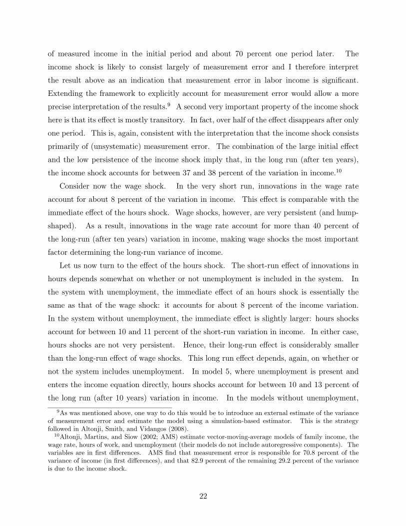
of measured income in the initial period and about 70 percent one period later. The

income shock is likely to consist largely of measurement error and I therefore interpret

the result above as an indication that measurement error in labor income is signi�cant.

Extending the framework to explicitly account for measurement error would allow a more

precise interpretation of the results.9 A second very important property of the income shock

here is that its e�ect is mostly transitory. In fact, over half of the e�ect disappears after only

one period. This is, again, consistent with the interpretation that the income shock consists

primarily of (unsystematic) measurement error. The combination of the large initial e�ect

and the low persistence of the income shock imply that, in the long run (after ten years),

the income shock accounts for between 37 and 38 percent of the variation in income.10

Consider now the wage shock. In the very short run, innovations in the wage rate

account for about 8 percent of the variation in income. This e�ect is comparable with the

immediate e�ect of the hours shock. Wage shocks, however, are very persistent (and hump-

shaped). As a result, innovations in the wage rate account for more than 40 percent of

the long-run (after ten years) variation in income, making wage shocks the most important

factor determining the long-run variance of income.

Let us now turn to the e�ect of the hours shock. The short-run e�ect of innovations in

hours depends somewhat on whether or not unemployment is included in the system. In

the system with unemployment, the immediate e�ect of an hours shock is essentially the

same as that of the wage shock: it accounts for about 8 percent of the income variation.

In the system without unemployment, the immediate e�ect is slightly larger: hours shocks

account for between 10 and 11 percent of the short-run variation in income. In either case,

hours shocks are not very persistent. Hence, their long-run e�ect is considerably smaller

than the long-run e�ect of wage shocks. This long run e�ect depends, again, on whether or

not the system includes unemployment. In model 5, where unemployment is present and

enters the income equation directly, hours shocks account for between 10 and 13 percent of

the long run (after 10 years) variation in income. In the models without unemployment,

9As was mentioned above, one way to do this would be to introduce an external estimate of the varianceof measurement error and estimate the model using a simulation-based estimator. This is the strategyfollowed in Altonji, Smith, and Vidangos (2008).10Altonji, Martins, and Siow (2002; AMS) estimate vector-moving-average models of family income, the

wage rate, hours of work, and unemployment (their models do not include autoregressive components). Thevariables are in �rst di�erences. AMS �nd that measurement error is responsible for 70.8 percent of thevariance of income (in �rst di�erences), and that 82.9 percent of the remaining 29.2 percent of the varianceis due to the income shock.

22

hours become slightly more important: in model 3, for instance, they account for between

14 and 17 percent of the long-run variation in income.

The interpretation of hours shocks also depends on whether or not unemployment is

included. When unemployment is not included, changes in unemployment hours are likely

to be an important component of hours shocks. Therefore, the results from the models with

unemployment should be more informative. In these models in particular, innovations in

hours appear not to be very important. It is reasonable to expect, however, that explicitly

accounting for measurement error in income would reduce the role played by the income

shock in the very short run, magnifying the relative role played by hours shocks, at least in

the short run.

Perhaps the most interesting result from the analysis above regards the e�ect of the

unemployment shock on income. Consider model 5, where unemployment is allowed to

a�ect income directly, as well as through its e�ect on hours and the wage rate. In this

model, unemployment shocks account for less than 5 percent of the income variation in

the very short run, and for about 10 percent in the long run (10 years after the shocks).

The e�ect of the unemployment shock is small in the short run because the size of the

unemployment shock is small (i.e., the estimated variance of the error in the unemployment

equation is small). On the other hand, the importance of the unemployment shock increases

with time, because the unemployment shock has a very persistent e�ect on income. As was

discussed above, the reason for the high degree of persistence of unemployment shocks is

that lagged unemployment (lagged by one period) has a large, negative, and very persistent

e�ect on the wage rate, which translates into a persistent e�ect on income.11 12

Finally, I brie y discuss the results that would obtain from the two alternative speci�-

cations discussed above: the speci�cation with moving-average errors and the speci�cation

with �xed e�ects. Consider �rst the instrumental-variables estimates presented in Table 2,

where the errors in models 1 and 2 follow MA(1) processes. The main implications of those

estimates for the behavior of income over time are as follows. In model 1, the income and

wage shocks have essentially the same e�ect as in the analysis above. The hours shock,

11If unemployment is left out of the wage equation, the persistence of the e�ect of the unemploymentshock on income essentially vanishes.12AMS �nd that the long-run e�ect of innovations in unemployment on income is near zero. In their

�ndings, even after only two years, a shock to unemployment of the head of the household has essentially noe�ect on income. In their models, the wage depends on lagged values of itself only; in particular, it is notallowed to depend on current or lagged values of unemployment. Their analysis thus does not capture thepersistent e�ect of unemployment on the wage rate.

23

on the other hand, behaves very similarly to the wage shock: the response of income is

hump-shaped, and the e�ect of the shock is very persistent. As a result, although in the

short run the income shock accounts for almost 90 percent of the income variation, in the

long run, each shock accounts for roughly one third of the variation in income. In model

2, by contrast, hours have essentially no e�ect on income; innovations in hours account for

less than 2 percent of the variation in income in both the short and long run. This result is

not very sensible and is due to the fact that the estimated coe�cient on hours in the income

equation in model 2 is close to zero.

Consider now the GMM estimates presented in Table 3 for models 1-6 with �xed e�ects,

estimated in �rst di�erences. The results from Table 3 have the following implications.

First of all, no shock has a permanent e�ect. The e�ect of all shocks is transitory and

vanishes completely after four periods. Second, the wage shock has essentially no e�ect on

income. In both the short and long run, the wage shock accounts for less than 1 percent of

the variation in income. The reason for these results is that the estimated coe�cient on the

wage in the income equation is close to zero in almost all models, as was discussed above.

Third, the income shock continues to behave as before. Consequently, the income shock

accounts for almost 90 percent of the short-run variation of income, and almost 85 percent

of its long-run variance.13 Finally, unemployment shocks account for about 6 percent of the

short-run variation and 9 percent of the long-run variation, while hours account for about

5 percent of the short-run variation and 6 percent of the long-run variation. As discussed

above, the small coe�cient on the wage in the income equation is problematic and is likely to

be caused by a weak instruments problem and by time inconsistencies in the measurement of

income and wages. Consequently, I stick to the estimation in levels presented above, which

looks more robust.

8 Conclusions

This paper studies variation in individual labor income over time using an extended panel

vector autoregression (PVAR) framework in income, the wage rate, hours of work, and hours

of unemployment. For consistency with the income dynamics literature, all variables used

are residuals from \Mincer-type" regressions. The framework is used to investigate how

much of the residual variation in labor income is due to residual variation in the wage rate,

13These results are quite similar to AMS, who also work with the variables in �rst di�erences.

24

work hours, and hours of unemployment. I also explore the dynamic e�ects of unanticipated

changes in each of the variables in the system, investigate their interactions, and assess their

relative importance in the determination of short-run and long-run income movements.

I �nd that, in the very short run, most of the variation in labor income is due to a factor

other than innovations in the wage rate, hours, or unemployment. Measurement error is

likely to be a major component of this factor, but the factor might also re ect unexpected

changes in non-wage labor income such as bonuses and commissions, and the fact that for

salaried workers the PSID wage measure is constructed using schedules with a �xed number

of hours. Most of the e�ect of this factor (which includes measurement error) is short-lived

and accounts for 37 - 38 percent of (residual) income variation in the long run. I also �nd

that, in the short run, innovations in the wage rate and work hours have a very similar e�ect

on income, conditional on unemployment. Wage innovations, however, are very persistent,

while the e�ect of changes in hours is mostly transitory. As a result, the wage rate is the

most important factor in the determination of (residual) income movements in the long run,

explaining more than 40 percent of the variation. Hours, by contrast, are responsible for only

10-13 percent of the long-run variance. Finally, I �nd that innovations in unemployment

have a relatively small, but very persistent e�ect on income. In the long run, they account

for 10 percent of the variation in income. The persistence of the e�ect of unemployment on

income is due to a large, negative, and very persistent e�ect of unemployment on the wage

rate.

The multivariate approach pursued in this paper stands in contrast with most of the

existing empirical literature on income dynamics, which studies income variation over time

without regard to income components or to speci�c factors that drive the income uctua-

tions. The approach followed here o�ers several advantages: (i) It allows me to distinguish

speci�c sources of income variation. In this paper I consider wage shocks, hours shocks,

unemployment shocks, and shocks to non-wage labor income (including measurement error).

It would be straightforward to incorporate additional shocks, such as health shocks; (ii) It

allows di�erent types of shocks to have di�erent dynamic properties and di�erent e�ects on

income. For instance, the results show that wage shocks are very persistent, while hours

shocks are mostly transitory. Consequently, factors that a�ect the wage rate are likely to

have a long-lasting e�ect on income, while factors that a�ect only hours are likely to have

only short-lived e�ects; (iii) It allows me to investigate the dynamic interactions among dif-

25

ferent shocks. One example are unemployment shocks, which are seen to have a long-lasting

e�ect on income because of their persistent e�ect on the wage rate. One could also use

this framework to investigate the e�ect of, for instance, health shocks on income, and their

dynamic interactions with hours, the wage rate, and employment status; (iv) It allows me to

decompose the variation in income at di�erent horizons into parts attributable to di�erent

shocks. This decomposition provides useful information about the role that di�erent shocks

play for income distribution and inequality; (v) Finally, the multivariate approach can also

be advantageous when using the income process as an input to decision models, as used in

the consumption-saving literature, or in macroeconomics or public �nance. Speci�cally, this

framework allows speci�cations in which agents condition their expectations of future income

on variables such as health and employment status, which contain important information

about future income.

Although this paper illustrates important advantages of taking a multivariate approach

to study uctuations in labor income, the work presented here has some important limita-

tions. First, as discussed above, measurement error is likely to be an important component

of the income shock considered in the PVAR system. A more complete analysis must

explicitly account for measurement error and distinguish it from actual innovations to non-

wage labor income. Second, variables such as labor income, the wage rate, work hours,

and unemployment are likely to be importantly in uenced by unobservable characteristics

of individuals such as di�erent preferences over work and leisure as well as ability and pro-

ductivity in the labor market. Such unobservable factors should be accounted for in a

exible manner. Third, the only sources of risk to labor income considered in this paper

are unemployment and unanticipated shocks to the wage rate, hours of work, and non-wage

labor income. There are additional sources of risk that are also likely to be important and

should be included in a more complete analysis, including disability and other health-related

shocks. Fourth, this paper does not study the income or wage e�ects of discrete events such

as job changes or accidents. Illness and unemployment could also be modeled as discrete

events. Altonji, Smith, and Vidangos (2008) addresses some of the above limitations.14

Finally, it was claimed above that the multivariate approach can be of value when using the

income process as an input to decision models. This is explored in Vidangos (2008), which

14They estimate a joint model of earnings, employment, job changes, wages, and work hours. The modelaccounts for measurement error and multiple sources of permanent unobserved heterogeneity. In additionto wage shocks and hours shocks, earnings are a�ected by employment and job change shocks.

26

studies the implications of a related multivariate model of family income{which allows for

unemployment, disability, health, and wage shocks{for precautionary behavior and welfare

in the context of a lifecycle consumption model.

27

9 References

Abowd, J.M. and Card, D.E. (1987). \Intertemporal labor supply and long-term employ-

ment contracts." American Economic Review, 77(1), 50-68.

Abowd, J.M. and Card, D.E. (1989). \On the covariance structure of hours and earnings

changes." Econometrica, 57(2), 411-445.

Aiyagari, S.R. (1994). \Uninsured idiosyncratic risk and aggregate saving." Quarterly

Journal of Economics 109, 659-684.

Altonji, J.G., Martins, A.P., and Siow, A. (2002). \Dynamic factor models of consump-

tion, hours, and income." Research in Economics, 56, 3-59.

Altonji, J.G., Smith Jr., A.A., and Vidangos, I. (2008). \Modeling Earnings Dynamics."

Unpublished Manuscript. Yale University and Federal Reserve Board.

Arellano, M. and Bond, S.R. (1991). \Some tests of speci�cation for panel data: Monte

Carlo evidence and an application to employment equations." Review of Economic Studies,

58, 277-297.

Arellano, M. and Bover, O. (1995). \Another look at the instrumental-variable estima-

tion of error-components models." Journal of Econometrics, 68, 29-52.

Baker, M. (1997). \Growth-rate heterogeneity and the covariance structure of life cycle

earnings." Journal of Labour Economics, 15(2), 338-375.

Baker, M. and Solon, G. (2003). \Earnings dynamics and inequality among Canadian

men, 1976-1992: evidence from longitudinal income tax records." Journal of Labor Eco-

nomics 21(2), 289-321.

Binder, M., Hsiao, C., and Pesaran, M.H. (2005). \Estimation and Inference in Short

Panel Vector Autoregressions with Unit Roots and Cointegration", Econometric Theory,

21(4), 795-837.

Blundell, R.W. and Bond, S.R. (1998). \Initial conditions and moment restrictions in

dynamic panel data models." Journal of Econometrics, 87, 115-143.

Casta~neda, A., D��az-Gim�enez, J., and R��os-Rull V. (2003). \Accounting for the U.S.

Earnings and Wealth Inequaility." Journal of Political Economy, 111(4), 818-857.

Deaton, A. (1991). \Saving and liquidity constraints." Econometrica, 59(5), 1221-1248.

Geweke, J. and Keane, M. (2000). \An empirical analysis of earnings dynamics among

men in the PSID: 1968-1989." Journal of Econometrics, 96, 293-356.

Guvenen, F. (2007). \Learning Your Earning: Are Labor Income Shocks Really Very

28

Persistent?" American Economic Review 97(3), 687-712.

Haider, S.J. (2001). \Earnings Instability and Earnings Inequality of Males in the United

States: 1967-1991." Journal of Labor Economics, 19(4), 799-836.

Hause, J.C. (1980). \The �ne structure of earnings and the on-the-job training hypoth-

esis." Econometrica, 48(4), 1013-1029.

Heaton, J. and Lucas, D.J. (1996). \Evaluating the e�ects of incomplete markets on

risk sharing and asset pricing." Journal of Political Economy, 104(3), 443-487.

Holtz-Eakin, D., Newey, W., and Rosen, H.S. (1988). \Estimating vector autoregressions

with panel data." Econometrica, 56(6), 1371-1395.

Imrohoroglu, A. (1989). \Cost of Business Cycles with Indivisibilities and Liquidity

Constraints." Journal of Political Economy, 97(6), 1364-1383.

Krusell, P. and Smith Jr., A . A. (1998). \Income and Wealth Heterogeneity in the

Macroeconomy." Journal of Political Economy, 106(5), 867-896.

Krusell, P. and Smith Jr., A . A. (1999). \On the welfare e�ects of eliminating business

cycles." Review of Economic Dynamics 2, 254-272.

Lillard, L. and Weiss, Y. (1979). \Components of variation in panel earnings data:

American scientists 1960-1970." Econometrica 47(2), 437-454.

Lillard, L. and Willis, R. (1978). \Dynamic aspects of earning mobility." Econometrica

46(5), 985-1012.

Low, H., Meghir, C., and Pistaferri, L. (2006). \Wage risk, employment risk, and

precautionary saving." Unpublished Manuscript. Cambridge University, University College

London, and Stanford University.

MaCurdy, T.E. (1982). \The use of time series processes to model the error structure

of earnings in a longitudinal data analysis." Journal of Econometrics, 18, 83-114.

Meghir, C. and Pistaferri, L. (2004). \Income variance dynamics and heterogeneity."

Econometrica, 72(1), 1-32.

Storesletten, K., Telmer, C., and Yaron, A. (2001a). \The Welfare Costs of Business

Cycles Revisited: Finite Lives and Cyclical Variation in Idiosyncratic Risk." European

Economic Review, 45, 1311-1339.

Storesletten, K., Telmer, C., and Yaron, A. (2001b). \How Important are Idiosyncratic

Shocks? Evidence from Labor Supply." American Economic Review (Papers and Proceed-

ings), 91, 413-417.

29

Storesletten, K., Telmer, C., and Yaron, A. (2007). \Asset Pricing with Idiosyncratic

Risk and Overlapping Generations." Review of Economic Dynamics, 10(4), 519-548.

Storesletten, K., Telmer, C., and Yaron, A. (2004a). \Consumption and Risk Sharing

Over the Life Cycle." Journal of Monetary Economics, 51(3), 609-633.

Storesletten, K., Telmer, C., and Yaron, A. (2004b). \Cyclical Dynamics in Idiosyncratic

Labor Market Risk." Journal of Political Economy, 112(3), 695-717.

Telmer, C. (1993). \Asset-Pricing Puzzles and Incomplete Markets." Journal of Finance,

48(5), 1803-1832.

Topel, R. (1991). Speci�c Capital, Mobility, and Wages: Wages Rise with Job Seniority."

Journal of Political Economy, 99(1), 145-176.

Topel, R. and Ward, M. (1992). \Job Mobility and the Careers of Young Men." Quar-

terly Journal of Economics, 107(2), 439-479.

Vidangos, I. (2008). \Household Welfare, Precautionary Saving, and Social Insurance

under Multiple Sources of Risk." Unpublished Manuscript. Federal Reserve Board.

30

31

Table 1 Pooled Least Squares Estimates of Models 1-6. Model 1 Model 2 Model 3 Model 4 Model 5 Model 6

Income Equation

Waget 0.4151 (0.0239) *0.000

0.4151 (0.0239) *0.000

0.3650 (0.0248) *0.000

0.3358 (0.0268) *0.000

0.3637 (0.0231) *0.000

0.3650 (0.0248) *0.000

Hourst 0.3315 (0.0350) *0.000

0.3315 (0.0350) *0.000

0.3240 (0.0370) *0.000

0.3417 (0.0466) *0.000

0.2903 (0.0343) *0.000

0.3240 (0.0370) *0.000

Unemploymentt

-0.5530 (0.0854) *0.000

Incomet-1 0.5541 (0.0245) *0.000

0.5541 (0.0245) *0.000

0.4249 (0.0232) *0.000

0.4332 (0.0223) *0.000

0.4222 (0.0222) *0.000

0.4249 (0.0232) *0.000

Incomet-2

0.1938 (0.0170) *0.000

0.1916 (0.0176) *0.000

0.1961 (0.0168) *0.000

0.1938 (0.0170) *0.000

Hourst-1

-0.0269 (0.0244) *0.270

Hourst-2

-0.0164 (0.0160) *0.304

Waget-1

0.0405 (0.0232) *0.081

Waget-2

-0.0147 (0.0194) *0.448

Root MSE 0.1732 0.1732 0.1684 0.1682 0.1663 0.1684 R-Squared 0.8410 0.8410 0.8510 0.8514 0.8547 0.8510 Robust standard errors are in parentheses. Asterisks (*) denote p values.

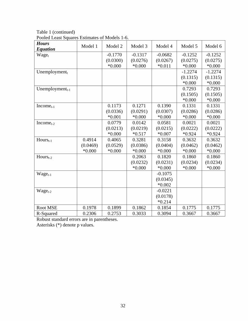
32

Table 1 (continued) Pooled Least Squares Estimates of Models 1-6. Hours Equation Model 1 Model 2 Model 3 Model 4 Model 5 Model 6

Waget

-0.1770 (0.0300) *0.000

-0.1317 (0.0276) *0.000

-0.0682 (0.0267) *0.011

-0.1252 (0.0275) *0.000

-0.1252 (0.0275) *0.000

Unemploymentt

-1.2274 (0.1315) *0.000

-1.2274 (0.1315) *0.000

Unemploymentt-1

0.7293 (0.1505) *0.000

0.7293 (0.1505) *0.000

Incomet-1

0.1173 (0.0336) *0.001

0.1271 (0.0291) *0.000

0.1390 (0.0307) *0.000

0.1331 (0.0286) *0.000

0.1331 (0.0286) *0.000

Incomet-2

0.0779 (0.0213) *0.000

0.0142 (0.0219) *0.517

0.0581 (0.0215) *0.007

0.0021 (0.0222) *0.924

0.0021 (0.0222) *0.924

Hourst-1 0.4914 (0.0469) *0.000

0.4065 (0.0529) *0.000

0.3281 (0.0386) *0.000

0.3158 (0.0404) *0.000

0.3632 (0.0462) *0.000

0.3632 (0.0462) *0.000

Hourst-2

0.2063 (0.0232) *0.000

0.1820 (0.0231) *0.000

0.1860 (0.0234) *0.000

0.1860 (0.0234) *0.000

Waget-1

-0.1075 (0.0345) *0.002

Waget-2

-0.0221 (0.0178) *0.214

Root MSE 0.1978 0.1899 0.1862 0.1854 0.1775 0.1775 R-Squared 0.2306 0.2753 0.3033 0.3094 0.3667 0.3667 Robust standard errors are in parentheses. Asterisks (*) denote p values.

33

Table 1 (continued) Pooled Least Squares Estimates of Models 1-6. Wage Equation Model 1 Model 2 Model 3 Model 4 Model 5 Model 6

Waget-1 0.9014 (0.0111) *0.000

0.9014 (0.0111) *0.000

0.6078 (0.0285) *0.000

0.4321 (0.0261) *0.000

0.6038 (0.0284) *0.000

0.6038 (0.0284) *0.000

Waget-2

0.2381 (0.0300) *0.000

0.2108 (0.0225) *0.000

0.2385 (0.0297) *0.000

0.2385 (0.0297) *0.000

Waget-3

0.1070 (0.0186) *0.000

0.1102

(0.0185) *0.000

0.1102 (0.0185) *0.000

Unemploymentt-1

-0.2845 (0.0677) *0.000

-0.2845 (0.0677) *0.000

Incomet-1

0.3724 (0.0258) *0.000

Incomet-2

-0.0699 (0.0161) *0.000

Hourst-1

-0.1778 (0.0340) *0.000

Hourst-2

-0.0264 (0.0158) *0.095

Root MSE 0.1732 0.1732 0.1619 0.1487 0.1613 0.1613 R-Squared 0.7927 0.7927 0.8227 0.8483 0.8241 0.8241 Unemployment Equation

Unemploymentt-1

0.3689 (0.0502) *0.000

0.3689 (0.0502) *0.000

Unemploymentt-2

0.0988 (0.0411) *0.017

0.0988 (0.0411) *0.017

Unemploymentt-3

0.1073 (0.0446) *0.017

0.1073 (0.0446) *0.017

Root MSE 0.0429 0.0429 R-Squared 0.2336 0.2336 Robust standard errors are in parentheses. Asterisks (*) denote p values.

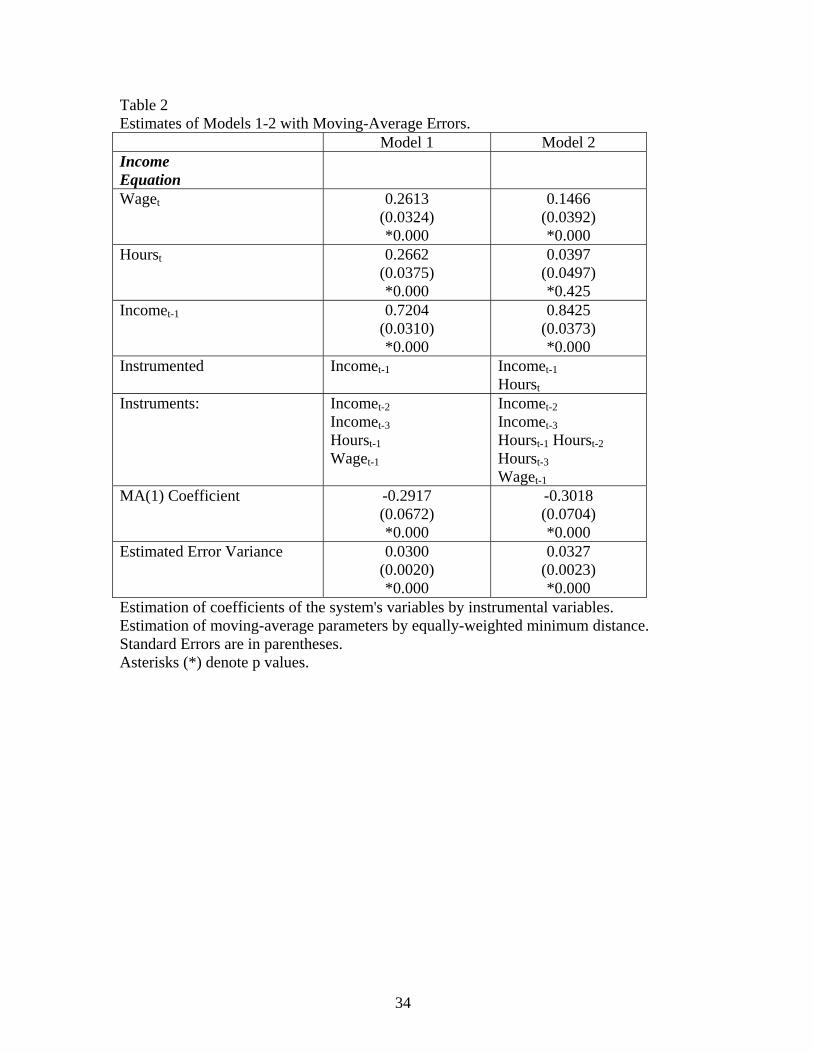
34

Table 2 Estimates of Models 1-2 with Moving-Average Errors. Model 1 Model 2 Income Equation

Waget 0.2613 (0.0324) *0.000

0.1466 (0.0392) *0.000

Hourst 0.2662 (0.0375) *0.000

0.0397 (0.0497) *0.425

Incomet-1 0.7204 (0.0310) *0.000

0.8425 (0.0373) *0.000

Instrumented Incomet-1 Incomet-1 Hourst

Instruments: Incomet-2 Incomet-3 Hourst-1 Waget-1

Incomet-2 Incomet-3 Hourst-1 Hourst-2 Hourst-3 Waget-1

MA(1) Coefficient -0.2917 (0.0672) *0.000

-0.3018 (0.0704) *0.000

Estimated Error Variance 0.0300 (0.0020) *0.000

0.0327 (0.0023) *0.000

Estimation of coefficients of the system's variables by instrumental variables. Estimation of moving-average parameters by equally-weighted minimum distance. Standard Errors are in parentheses. Asterisks (*) denote p values.

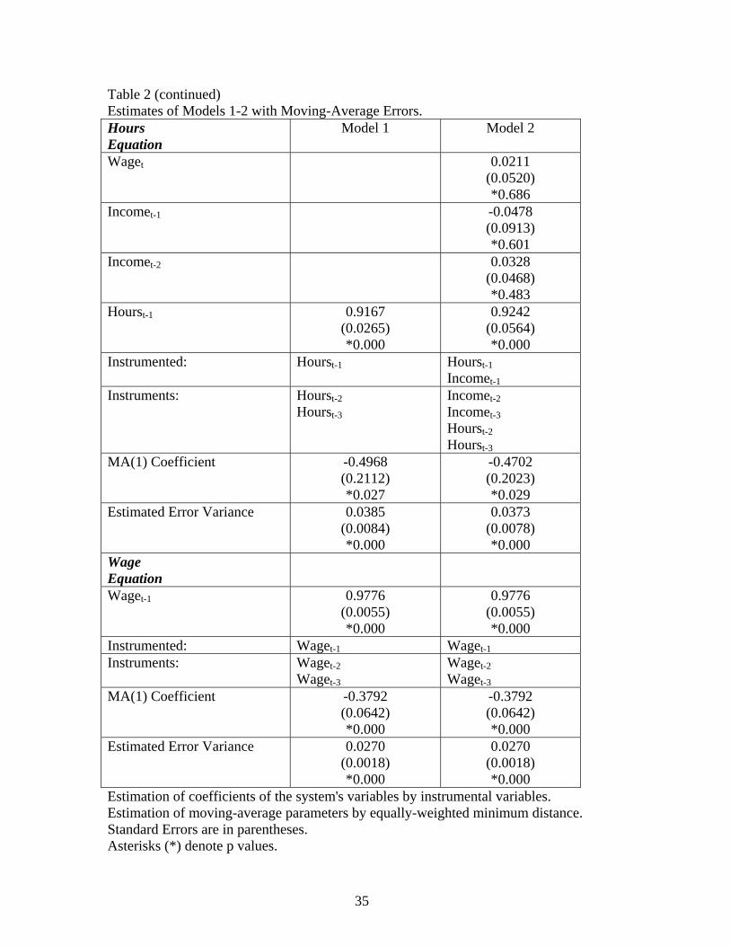
35

Table 2 (continued) Estimates of Models 1-2 with Moving-Average Errors. Hours Equation

Model 1 Model 2

Waget

0.0211 (0.0520) *0.686

Incomet-1

-0.0478 (0.0913) *0.601

Incomet-2

0.0328 (0.0468) *0.483

Hourst-1 0.9167 (0.0265) *0.000

0.9242 (0.0564) *0.000

Instrumented: Hourst-1 Hourst-1 Incomet-1

Instruments: Hourst-2 Hourst-3

Incomet-2 Incomet-3 Hourst-2 Hourst-3

MA(1) Coefficient -0.4968 (0.2112) *0.027

-0.4702 (0.2023) *0.029

Estimated Error Variance 0.0385 (0.0084) *0.000

0.0373 (0.0078) *0.000

Wage Equation

Waget-1 0.9776 (0.0055) *0.000

0.9776 (0.0055) *0.000

Instrumented: Waget-1 Waget-1 Instruments: Waget-2

Waget-3 Waget-2 Waget-3

MA(1) Coefficient -0.3792 (0.0642) *0.000

-0.3792 (0.0642) *0.000

Estimated Error Variance 0.0270 (0.0018) *0.000

0.0270 (0.0018) *0.000

Estimation of coefficients of the system's variables by instrumental variables. Estimation of moving-average parameters by equally-weighted minimum distance. Standard Errors are in parentheses. Asterisks (*) denote p values.

36

Table 3 Estimates of Models with Fixed Effects. Model 1 Model 2 Model 3 Model 4 Model 5 Model 6

Income Equation

Waget 0.0338 (0.0318) *0.287

0.0484 (0.0302) *0.109

0.0244 (0.0343) *0.477

0.1680 (0.0567) *0.003

0.0249 (0.0355) *0.483

0.0161 (0.0350) *0.646

Hourst 0.2902 (0.0542) *0.000

0.2638 (0.0586) *0.000

0.2846 (0.0657) *0.000

0.2848 (0.0686) *0.000

0.2365 (0.0712) *0.001

0.3002 (0.0738) *0.000

Unemploymentt

-0.6512 (0.1646) *0.000

Incomet-1 0.2967 (0.0437) *0.000

0.2502 (0.0426) *0.000

0.2911 (0.0557) *0.000

0.2533 (0.0472) *0.000

0.2987 (0.0580) *0.000

0.3092 (0.0588) *0.000

Incomet-2

0.0766 (0.0251) *0.002

0.0719 (0.0264) *0.006

0.0827 (0.0256) *0.001

0.0824 (0.0260) *0.002

Hourst-1

-0.0159 (0.0269) *0.554

Hourst-2

0.0008 (0.0162) *0.958

Waget-1

0.0016 (0.0295) *0.956

Waget-2

-0.0467 (0.0246) *0.058

Test for 1st order Serial Corr.

-10.13 *0.000

-10.21 *0.000

-9.41 *0.000

-9.29 *0.000

-9.11 *0.000

-9.33 *0.000

Test for 2nd order Serial Corr.

2.39 *0.017

2.10 *0.035

-0.84 *0.400

-1.21 *0.228

-1.13 *0.258

-0.93 *0.353

Estimation of all equations by linear GMM. Tests for serial correlation use the first-differenced residuals. See Arellano and Bond (1991). Standard Errors are in parentheses. Asterisks (*) denote p values.

37

Table 3 (continued) Estimates of Models with Fixed Effects. Model 1 Model 2 Model 3 Model 4 Model 5 Model 6

Hours Equation

Waget 0.0148 (0.0392) *0.706

0.0128 (0.0389) *0.742

-0.0105 (0.0630) *0.868

0.0376 (0.0381) *0.325

0.0376 (0.0381) *0.325

Unemploymentt -1.3842 (0.1252) *0.000

-1.3842 (0.1252) *0.000

Unemploymentt-1 0.1823 (0.1050) *0.083

0.1823 (0.1050) *0.083

Incomet-1 0.0516 (0.0625) *0.410

0.0477 (0.0660) *0.469

0.0592 (0.0405) *0.144

0.0209 (0.0643) *0.745

0.0209 (0.0643) *0.745

Incomet-2 0.0457 (0.0240) *0.056

0.0324 (0.0264) *0.219

0.0475 (0.0227) *0.036

0.0264 (0.0293) *0.368

0.0264 (0.0293) *0.368

Hourst-1 0.1248 (0.0341) *0.000

0.1190 (0.0337) *0.000

0.1370 (0.0356) *0.000

0.1302 (0.0326) *0.000

0.1318 (0.0370) *0.000

0.1318 (0.0370) *0.000

Hourst-2 0.0399 (0.0174) *0.022

0.0320 (0.0162) *0.048

0.0173 (0.0220) *0.433

0.0173 (0.0220) *0.433

Waget-1 -0.0491 (0.0347) *0.157

Waget-2 0.0119 (0.0246) *0.629

Test for 1st order Serial Corr.

-5.04 *0.000

-4.61 *0.000

-4.61 *0.000

-4.62 *0.000

-4.20 *0.000

-4.20 *0.000

Test for 2nd order Serial Corr.

1.72 *0.085

1.48 *0.140

0.36 *0.722

0.37 *0.709

0.26 *0.794

0.26 *0.794

Estimation of all equations by linear GMM. Tests for serial correlation use the first-differenced residuals. See Arellano and Bond (1991). Standard Errors are in parentheses. Asterisks (*) denote p values.

38

Table 3 (continued) Estimates of Models with Fixed Effects. Wage Equation Model 1 Model 2 Model 3 Model 4 Model 5 Model 6

Waget-1 0.2985 (0.0474) *0.000

0.2985 (0.0474) *0.000

0.4154 (0.0524) *0.000*

0.2409 (0.0351) *0.000

0.4145 (0.0527) *0.000

0.4145 (0.0527) *0.000

Waget-2

0.1409 (0.0326) *0.000

0.0825 (0.0241) *0.001

0.1429 (0.0324) *0.000

0.1429 (0.0324) *0.000

Waget-3

0.0293 (0.0222) *0.188

0.0333

(0.0222) *0.133

0.0333 (0.0222) *0.133

Unemploymentt-1

-0.3048 (0.1116) *0.006

-0.3048 (0.1116) *0.006

Incomet-1

0.3425 (0.0447) *0.000

Incomet-2

0.0023 (0.0198) *0.907

Hourst-1

-0.1438 (0.0407) *0.000

Hourst-2

-0.0179 (0.0164) *0.275

Test for 1st order Serial Corr.

-10.26 *0.000

-10.26 *0.000

-9.73 *0.000

-11.23 *0.000

-9.71 *0.000

-9.71 *0.000

Test for 2nd order Serial Corr.

2.94 *0.003

2.94 *0.003

-0.84 *0.399

-0.05 *0.964

-1.03 *0.304

-1.03 *0.304

Estimation of all equations by linear GMM. Tests for serial correlation use the first-differenced residuals. See Arellano and Bond (1991). Standard Errors are in parentheses. Asterisks (*) denote p values.

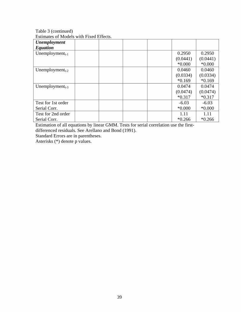
39

Table 3 (continued) Estimates of Models with Fixed Effects. Unemployment Equation

Unemploymentt-1

0.2950 (0.0441) *0.000

0.2950 (0.0441) *0.000

Unemploymentt-2

0.0460 (0.0334) *0.169

0.0460 (0.0334) *0.169

Unemploymentt-3

0.0474 (0.0474) *0.317

0.0474 (0.0474) *0.317

Test for 1st order Serial Corr. -6.03

*0.000 -6.03

*0.000 Test for 2nd order Serial Corr. 1.11

*0.266 1.11

*0.266 Estimation of all equations by linear GMM. Tests for serial correlation use the first-differenced residuals. See Arellano and Bond (1991). Standard Errors are in parentheses. Asterisks (*) denote p values.

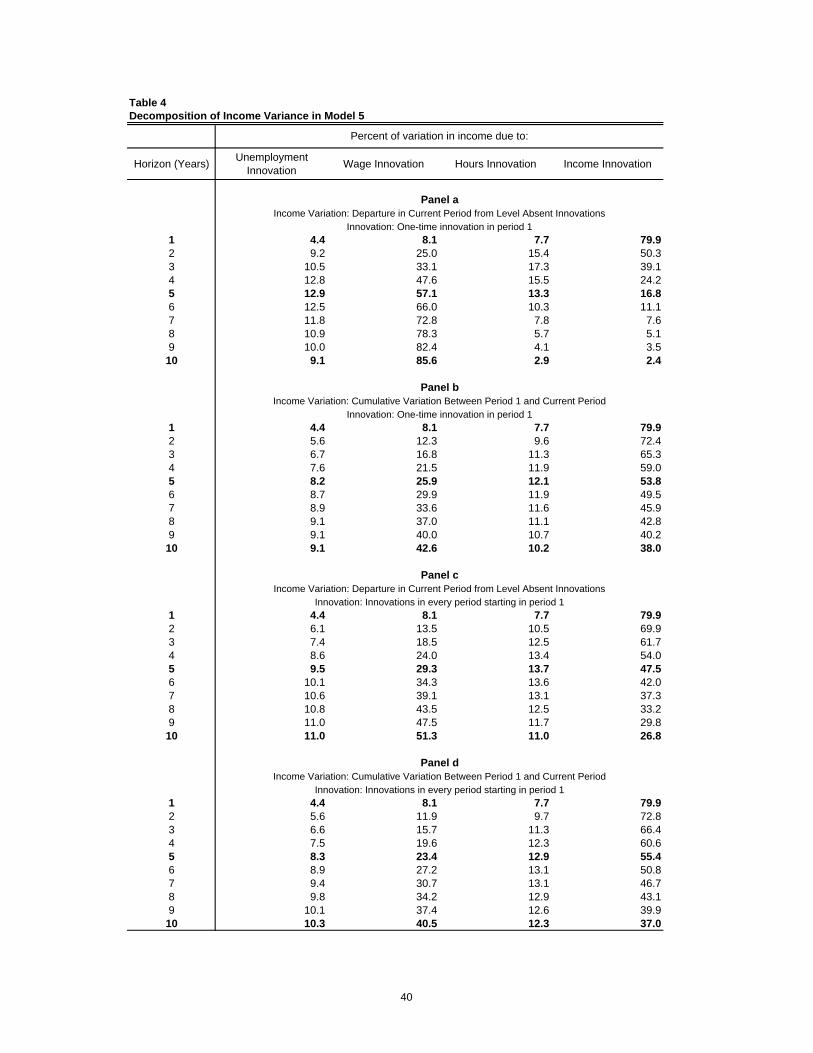
Table 4Decomposition of Income Variance in Model 5

Horizon (Years) Unemployment Innovation Wage Innovation Hours Innovation Income Innovation

1 4.4 8.1 7.7 79.92 9.2 25.0 15.4 50.33 10.5 33.1 17.3 39.14 12.8 47.6 15.5 24.25 12.9 57.1 13.3 16.86 12.5 66.0 10.3 11.17 11.8 72.8 7.8 7.68 10.9 78.3 5.7 5.19 10.0 82.4 4.1 3.510 9.1 85.6 2.9 2.4

1 4.4 8.1 7.7 79.92 5.6 12.3 9.6 72.43 6.7 16.8 11.3 65.34 7.6 21.5 11.9 59.05 8.2 25.9 12.1 53.86 8.7 29.9 11.9 49.57 8.9 33.6 11.6 45.98 9.1 37.0 11.1 42.89 9.1 40.0 10.7 40.210 9.1 42.6 10.2 38.0

1 4.4 8.1 7.7 79.92 6.1 13.5 10.5 69.93 7.4 18.5 12.5 61.74 8.6 24.0 13.4 54.05 9.5 29.3 13.7 47.56 10.1 34.3 13.6 42.07 10.6 39.1 13.1 37.38 10.8 43.5 12.5 33.29 11.0 47.5 11.7 29.810 11.0 51.3 11.0 26.8

1 4.4 8.1 7.7 79.92 5.6 11.9 9.7 72.83 6.6 15.7 11.3 66.44 7.5 19.6 12.3 60.65 8.3 23.4 12.9 55.46 8.9 27.2 13.1 50.87 9.4 30.7 13.1 46.78 9.8 34.2 12.9 43.19 10.1 37.4 12.6 39.910 10.3 40.5 12.3 37.0

Panel b

Panel cIncome Variation: Departure in Current Period from Level Absent Innovations

Innovation: Innovations in every period starting in period 1

Income Variation: Cumulative Variation Between Period 1 and Current PeriodInnovation: One-time innovation in period 1

Percent of variation in income due to:

Panel aIncome Variation: Departure in Current Period from Level Absent Innovations

Innovation: One-time innovation in period 1

Panel dIncome Variation: Cumulative Variation Between Period 1 and Current Period

Innovation: Innovations in every period starting in period 1

40

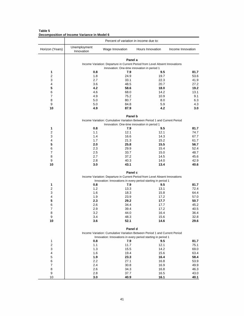
Table 5Decomposition of Income Variance in Model 6

Horizon (Years) Unemployment Innovation Wage Innovation Hours Innovation Income Innovation

1 0.8 7.9 9.5 81.72 1.8 24.9 19.7 53.63 2.7 33.1 22.3 41.94 3.6 48.5 20.7 27.25 4.2 58.6 18.0 19.26 4.6 68.0 14.2 13.17 4.9 75.2 10.9 9.18 5.0 80.7 8.0 6.39 5.0 84.8 5.9 4.310 4.9 87.9 4.2 3.0

1 0.8 7.9 9.5 81.72 1.1 12.1 12.1 74.73 1.4 16.6 14.3 67.74 1.7 21.3 15.2 61.75 2.0 25.8 15.5 56.76 2.3 29.9 15.4 52.47 2.5 33.7 15.0 48.78 2.7 37.2 14.5 45.69 2.8 40.3 14.0 42.910 3.0 43.1 13.4 40.6

1 0.8 7.9 9.5 81.72 1.2 13.3 13.1 72.43 1.6 18.3 15.8 64.44 1.9 23.9 17.2 57.05 2.3 29.2 17.7 50.76 2.6 34.4 17.7 45.27 2.9 39.4 17.2 40.58 3.2 44.0 16.4 36.49 3.4 48.3 15.6 32.810 3.6 52.1 14.6 29.6

1 0.8 7.9 9.5 81.72 1.1 11.7 12.1 75.13 1.3 15.5 14.2 69.04 1.6 19.4 15.6 63.45 1.9 23.3 16.4 58.46 2.2 27.1 16.8 53.97 2.4 30.8 16.9 49.98 2.6 34.3 16.8 46.39 2.8 37.7 16.5 43.010 3.0 40.9 16.1 40.1

Income Variation: Cumulative Variation Between Period 1 and Current PeriodPanel d

Innovation: Innovations in every period starting in period 1

Percent of variation in income due to:

Panel aIncome Variation: Departure in Current Period from Level Absent Innovations

Innovation: One-time innovation in period 1

Panel bIncome Variation: Cumulative Variation Between Period 1 and Current Period

Innovation: One-time innovation in period 1

Panel cIncome Variation: Departure in Current Period from Level Absent Innovations

Innovation: Innovations in every period starting in period 1

41

Table 6Decomposition of Income Variance in Model 3

Horizon (Years) Wage Innovation Hours Innovation Income Innovation

1 7.8 10.5 81.72 25.5 20.2 54.33 33.7 23.8 42.54 50.2 21.8 28.05 60.8 19.2 20.06 71.1 15.1 13.77 78.8 11.6 9.68 84.7 8.6 6.69 89.1 6.3 4.610 92.3 4.5 3.2

1 7.8 10.5 81.72 12.2 12.9 74.93 16.7 15.2 68.14 21.6 16.1 62.35 26.2 16.5 57.36 30.5 16.4 53.17 34.5 16.0 49.68 38.1 15.4 46.59 41.4 14.9 43.810 44.3 14.3 41.5

1 7.8 10.5 81.72 13.4 14.0 72.73 18.4 16.8 64.84 24.2 18.2 57.65 29.7 18.8 51.56 35.2 18.7 46.17 40.4 18.3 41.48 45.2 17.5 37.39 49.7 16.6 33.710 53.9 15.6 30.5

1 7.8 10.5 81.72 11.8 12.9 75.3 3 15.6 15.1 69.34 19.6 16.5 63.95 23.6 17.4 59.06 27.5 17.9 54.67 31.3 18.0 50.78 35.0 17.9 47.19 38.6 17.6 43.910 41.9 17.1 41.0

Income Variation: Cumulative Variation Between Period 1 and Current Period

Innovation: Innovations in every period starting in period 1

Innovation: One-time innovation in period 1

Panel d

Innovation: Innovations in every period starting in period 1

Panel aIncome Variation: Departure in Current Period from Level Absent Innovations

Innovation: One-time innovation in period 1

Panel bIncome Variation: Cumulative Variation Between Period 1 and Current Period

Panel cIncome Variation: Departure in Current Period from Level Absent Innovations

Percent of variation in income due to:

42

43

Figure 1 Income Response to Wage Shock in Models 1 – 4

Time

Model 1 Model 2 Model 3 Model 4

0 5 10 15 20 25 30

0

.02

.04

.06

.08

The figure shows the response of income to a one-time, one-standard-deviation wage shock at time t=1.

Figure 2 Income Response to Hours Shock in Models 1 - 4

Time

Model 1 Model 2 Model 3 Model 4

0 5 10 15 20 25 30

0

.02

.04

.06

.08

The figure shows the response of income to a one-time, one-standard-deviation hours shock at time t=1.

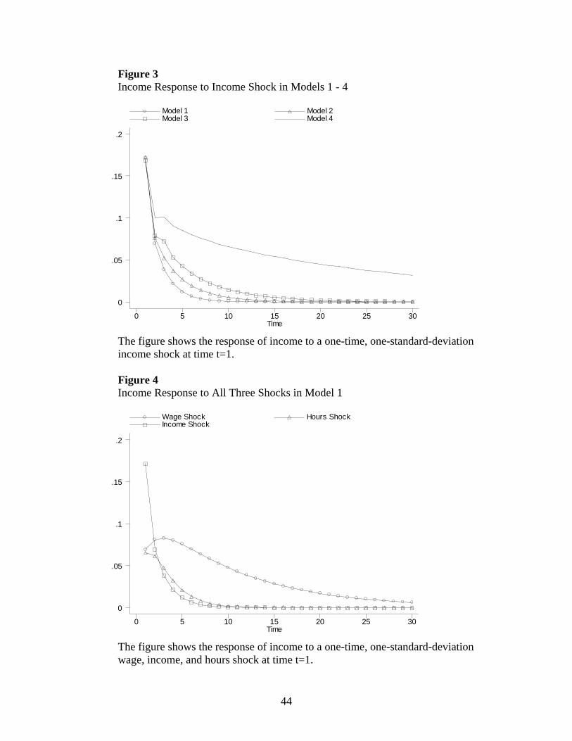
44

Figure 3 Income Response to Income Shock in Models 1 - 4

Time

Model 1 Model 2 Model 3 Model 4

0 5 10 15 20 25 30

0

.05

.1

.15

.2

The figure shows the response of income to a one-time, one-standard-deviation income shock at time t=1.

Figure 4 Income Response to All Three Shocks in Model 1

Time

Wage Shock Hours Shock Income Shock

0 5 10 15 20 25 30

0

.05

.1

.15

.2

The figure shows the response of income to a one-time, one-standard-deviation wage, income, and hours shock at time t=1.

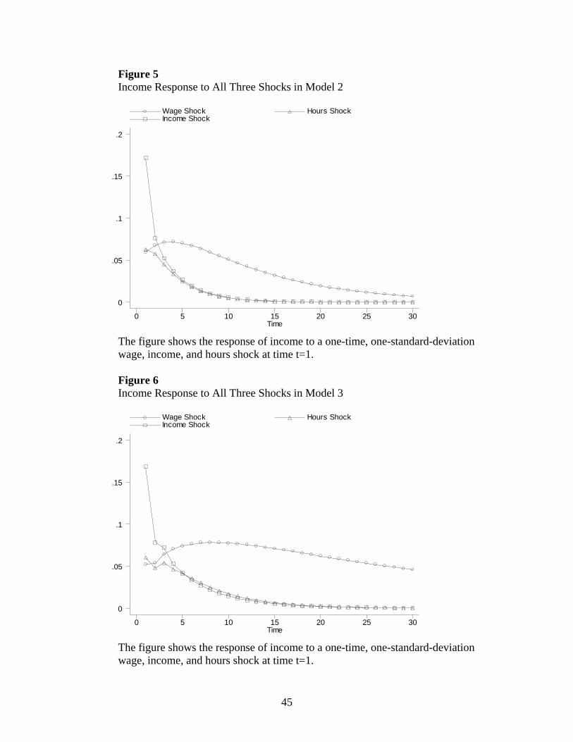
45

Figure 5 Income Response to All Three Shocks in Model 2

Time

Wage Shock Hours Shock Income Shock

0 5 10 15 20 25 30

0

.05

.1

.15

.2

The figure shows the response of income to a one-time, one-standard-deviation wage, income, and hours shock at time t=1.

Figure 6 Income Response to All Three Shocks in Model 3

Time

Wage Shock Hours Shock Income Shock

0 5 10 15 20 25 30

0

.05

.1

.15

.2

The figure shows the response of income to a one-time, one-standard-deviation wage, income, and hours shock at time t=1.

46

Figure 7 Income Response to All Three Shocks in Model 4 (unrestricted PVAR)

Time

Wage Shock Hours Shock Income Shock

0 5 10 15 20 25 30

0

.05

.1

.15

.2

The figure shows the response of income to a one-time, one-standard-deviation wage, income, and hours shock at time t=1.

Figure 8 Income Response to All Four Shocks in Model 5

Time

Unemployment Shock Wage Shock Hours Shock Income Shock

0 5 10 15 20 25 30

-.1

0

.1

.2

The figure shows the response of income to a one-time, one-standard-deviation unemployment hours, work hours, wage, and income shock at time t=1.

47

Figure 9 Income Response to All Four Shocks in Model 6

Time

Unemployment Shock Wage Shock Hours Shock Income Shock

0 5 10 15 20 25 30

0

.1

.2

The figure shows the response of income to a one-time, one-standard-deviation unemployment hours, work hours, wage, and income shock at time t=1.

Figure 10 Response of Wage and Hours to Unemployment Shock in Model 5

Time

Wage Hours

0 5 10 15 20 25 30

-.06

-.04

-.02

0

The figure shows the response of the wage and work hours to a one-time, one-standard-deviation unemployment hours shock at time t=1.

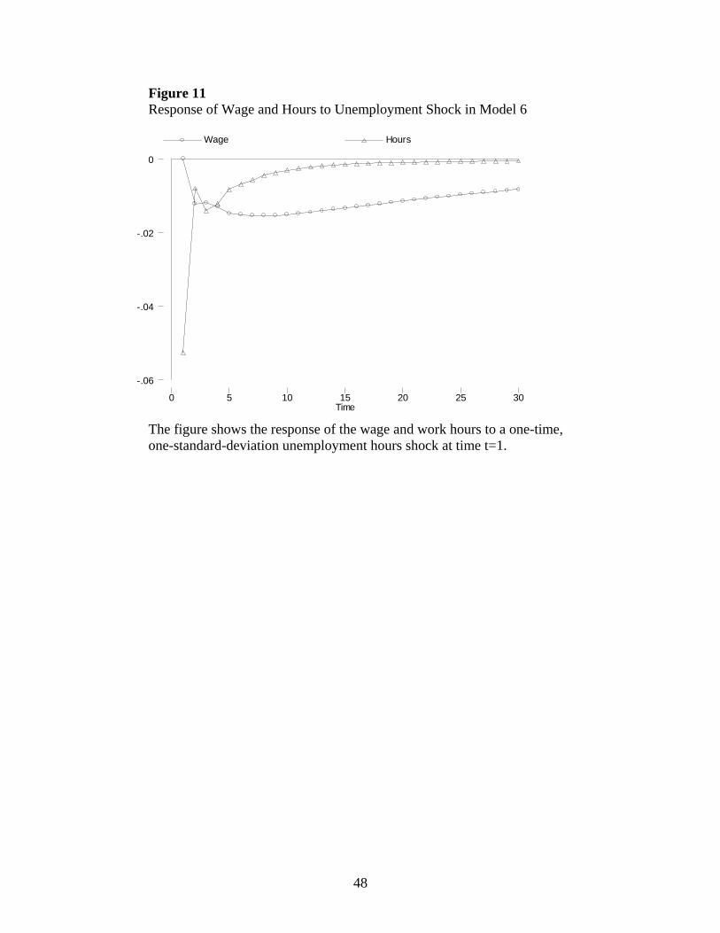
48

Figure 11 Response of Wage and Hours to Unemployment Shock in Model 6

Time

Wage Hours

0 5 10 15 20 25 30

-.06

-.04

-.02

0

The figure shows the response of the wage and work hours to a one-time, one-standard-deviation unemployment hours shock at time t=1.