Article Development of a 3D webGIS application for the

Article

Development of a 3D webGIS application for the visualization

of seismic risk on infrastructural work

Mauro Mazzei 1,*, Davide Quaroni 2

1 National Research Council, Istituto di Analisi dei Sistemi ed Informatica, LabGeoInf, Via dei Taurini, 19,

I-00185, Rome, Italy; [email protected] 2 National Research Council, LabGeoInf, Via dei Taurini, 19,I-00185, Rome, Italy; [email protected]

* Correspondence: [email protected]

Abstract: In this paper we describe the potentialities of a tool for the visualization of experimental

results directly on a three-dimensional model. The case study concerns the visualization of the re-

sults of a dynamic finite element analysis (FEA/FEM) applied to the calculation of seismic risk on

works belonging to the Italian infrastructural heritage, specifically bridges, viaducts and over-

passes. The project is based on finite element analysis performed on an exemplary set of 8 struc-

tures located on the Italian territory, performed by means of the open-source software framework

OpenSees, according to the guidelines indicated in the Technical Standards for Construction

NTC08. The application created for this project is classifiable as a webGIS, since all data are

georeferenced and visualized on a map through an application executed through a browser. The

graphical interface displays the interested works on the map of the Italian territory and allows to

select them by mouse click. Following the selection, a 3D rendering of the model of the work and

the surrounding terrain is shown, in which the results of the analysis are represented using color

gradients directly on the three-dimensional model. The necessary tools are present for the selection

of the type of result and for the animation in real time of the response of the work to the seismic

action. The 3D representation is freely navigable by the user thanks to intuitive tools of panning,

rotation and zoom through mouse and keyboard. The application takes advantage of HTML5, CSS

and Javascript to show graphical features such as Cartesian diagrams of accelerograms used in

modal analysis.

Keywords: web-GIS 3d; Seismic Analysis; Structural Analysis; FEA/FEM Analysis; OpenSees.

1. Introduction

Italy can count on a rich infrastructural heritage, made up of bridges, viaducts and

overpasses on both road and rail networks. Economic development is based on these in-

frastructures and inevitably relies on the transport sector to move goods and raw mate-

rials that are fundamental to all sectors of the economy.

The safety of infrastructural works, of course, is not only important for commercial

purposes but it is especially important for the safety of millions of people who travel on

them every day; tragedies such as the recent collapse of the Morandi bridge in Genoa

have shown that monitoring and complete knowledge of the structural elements of these

works is of fundamental importance.

One of the major risks in the country is seismic: Italy is one of the countries with

high seismic risk, especially along the Apennines, and this requires extreme caution in

the design and maintenance of infrastructure works, which are by their nature vulnerable

to ground movements caused by an earthquake. For this reason, in 2008 the Technical

Standards for Construction [4] were introduced, then updated in 2018, in which among

other things are defined the criteria with which to perform analysis for seismic risk.

Civil and structural engineers who deal with these issues rely on finite state mod-

eling software, or FEA/FEM (Finite Element Analysis/Finite Element Method), to perform

Preprints (www.preprints.org) | NOT PEER-REVIEWED | Posted: 16 November 2021

© 2021 by the author(s). Distributed under a Creative Commons CC BY license.

doi:10.20944/preprints202111.0275.v1

http://creativecommons.org/licenses/by/4.0/

https://doi.org/10.20944/preprints202111.0275.v1

the necessary calculations [2]; these software start from a three-dimensional model of the

system to be analyzed, dividing it into small parts for which it is easier to perform the

calculations, then arriving at the final result [22-24].

One of these software is OpenSees [5], created by the University of Berkley, which is

proposed as an alternative to commercial software available on the market.

The project described in this paper proposes to be a valid help in the elaboration and

visualization of the results of these analyses, presenting them in the form of a color gra-

dient applied directly to a three-dimensional model of the work.

In order to insert the model even better in its natural context, it was decided to add a

model of the surrounding terrain, with elevation data taken from the DEM (Digital Ele-

vation Model) TINITALY/01 of INGV [6], and textures obtained from satellite images[3].

In recent years there has been a growth in the proposal and use of web platforms,

executed by the browser already installed on your computer, because this leads to sig-

nificant advantages, such as independence from the operating system and type of hard-

ware, the execution of complex calculations on remote servers, the lack of installers that

could lead to attacks by malicious software. For this reason it was decided to follow this

path, creating a cartographic web application in which data are georeferenced and 3D

rendering is done client-side through the Three.js Javascript library [9-12].

2. Materials and Methods

2.1. GIS system

GIS (Geographic Information System) systems are computerized information sys-

tems that allow the acquisition, processing and display of georeferenced spatial data. The

computer system is therefore able to associate data with their position on the earth's

surface, to allow their processing, aggregation, search and display on a map [16].

The main use of GIS systems is in digital cartography, in the study and representa-

tion of natural and human phenomena in relation to the territory.

GIS systems are composed of a hardware part, consisting of processors in which

data are stored on file systems or databases, and a software part, which is responsible for

acquiring any input data, perform processing and interface with the user through the UI

(user interface).

2.2. WebGIS system

In recent years the internet connection has expanded considerably, and nowadays it

is difficult to find a device (PC, tablet, smartphone) that is not connected to the network.

For this reason, in addition to desktop GIS applications [1], i.e. installed and executed

locally on the device, more and more cartographic applications executed through a

browser, the so-called webGIS, have become popular.

WebGIS are based on a client-server architecture: the client, running on a browser,

has the task of displaying geographical information and acquiring input data and com-

mands; the server, on the other hand, processes the input data and provides the client

with the required data in the form of numerical data, vector or raster geographical data.

The web approach has significant advantages:

• no need to install software locally, with all the problems of hardware and software

incompatibility that this might entail;

• development and maintenance of a single version of the software: the browsers on

which it runs are an additional level of abstraction, and it is up to them to manage

the differences, for example, between Windows, Linux, MacOS environments;

• ability to access the software from any device, anywhere in the world, as long as it

has an internet connection: most webGIS offer authentication features, allowing ac-

cess to personal data and settings once logged in;

• execution of any processing on the server hardware instead of on the user's device:

this allows, especially in case of heavy processing, to launch their execution, dis-

Preprints (www.preprints.org) | NOT PEER-REVIEWED | Posted: 16 November 2021 doi:10.20944/preprints202111.0275.v1


connect from the application and return to check the status of processing, without

keeping local resources busy [36].

2.3. Data types

Working with graphical representations of data, GIS systems must be able to handle

various formats in which these may be presented. The two main categories are vector

data and raster data.

2.3.1 Vector data

Vector data consists of vectors containing numerical information about the posi-

tioning of the various points that make up the geographic data. These can be point, linear

or polygonal data. They are usually composed of two parts: the geographic vector itself,

used by the GIS system to position the geometry on the map, and a set of attributes as-

sociated with the geometry, which can be displayed for example when selecting the point

of interest.

Figure 1. point-type vector geometry

.

Figure 2. linear type vector geometry



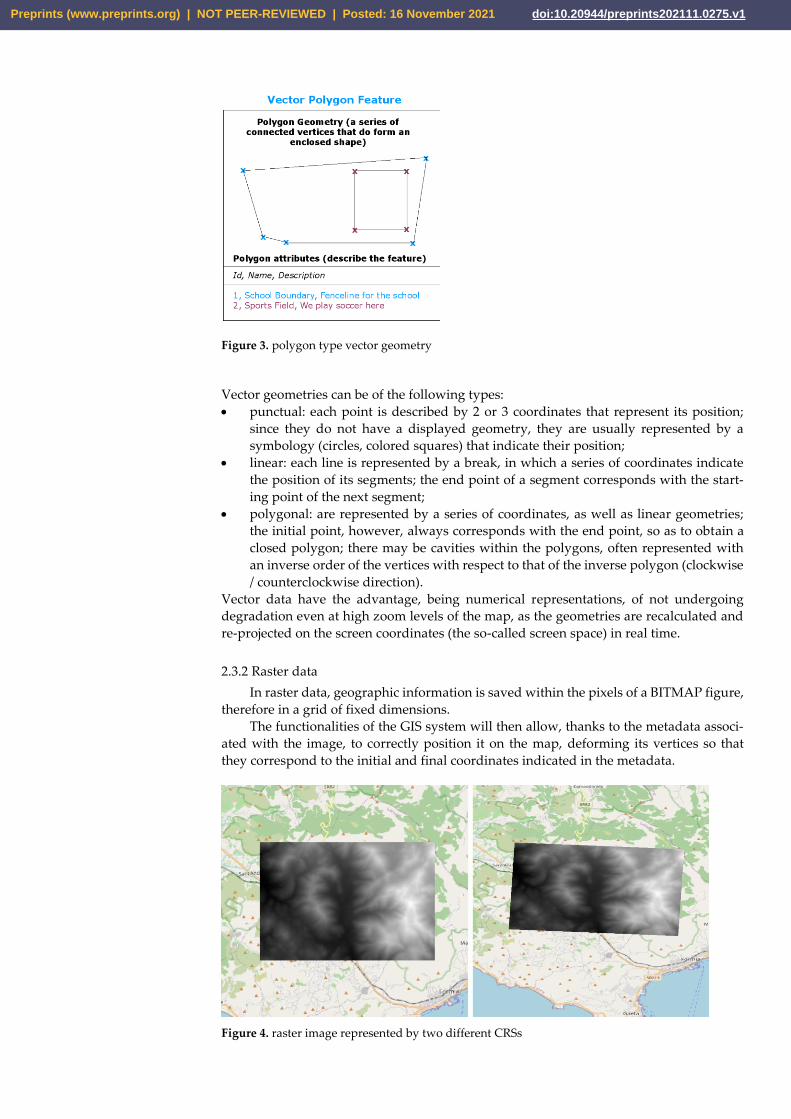
Figure 3. polygon type vector geometry

Vector geometries can be of the following types:

• punctual: each point is described by 2 or 3 coordinates that represent its position;

since they do not have a displayed geometry, they are usually represented by a

symbology (circles, colored squares) that indicate their position;

• linear: each line is represented by a break, in which a series of coordinates indicate

the position of its segments; the end point of a segment corresponds with the start-

ing point of the next segment;

• polygonal: are represented by a series of coordinates, as well as linear geometries;

the initial point, however, always corresponds with the end point, so as to obtain a

closed polygon; there may be cavities within the polygons, often represented with

an inverse order of the vertices with respect to that of the inverse polygon (clockwise

/ counterclockwise direction).

Vector data have the advantage, being numerical representations, of not undergoing

degradation even at high zoom levels of the map, as the geometries are recalculated and

re-projected on the screen coordinates (the so-called screen space) in real time.

2.3.2 Raster data

In raster data, geographic information is saved within the pixels of a BITMAP figure,

therefore in a grid of fixed dimensions.

The functionalities of the GIS system will then allow, thanks to the metadata associ-

ated with the image, to correctly position it on the map, deforming its vertices so that

they correspond to the initial and final coordinates indicated in the metadata.

Figure 4. raster image represented by two different CRSs



In figure 4 you can see the same raster image displayed with two different CRS. On the

left the CRS used corresponds to that of the raster image, while on the right the GIS sys-

tem had to perform a deformation to adapt the CRS of the image to that of the project [7].

Figure 5. resolution of a raster image

Being composed of a limited number of pixels, raster data suffers from resolution loss

and grainy effects at high zoom levels; moreover, unlike vector data, they cannot usually

have multiple attributes associated with a single pixel. However, they are very useful

when one wants to represent complex phenomena that cannot be represented by point or

polygonal geometries [33-35].

2.4. Finite element analysis

Finite element analysis (FEM, Finite Elements Method, or more properly FEA, Finite

Elements Analysis), is a computational technique performed using computers, which

allows to study the structural behavior of a system. This tool is commonly used in engi-

neering to study the behavior of mechanical systems.

The analysis consists of creating a three-dimensional model (mesh) of the system to

be analyzed and subdividing it into many smaller elements of easy mathematical solu-

tion. The total result will be obtained by summing the results obtained on all the ele-

ments.

Figure 6. generation of a mesh from the geometry

A finite element analysis allows you to study how the system reacts to external stresses,

recording the displacements, deformations and stresses to which each part is subjected.



Figure 7. mesh deformation after analysis

2.4.1 Modal analysis with FEM method

Modal analysis is the study of the dynamic properties of structures under vibra-

tional excitation. It is performed on the linear elastic model, so elastic elements have also

been defined for curves. In structural engineering, modal analysis involves the use of

both, a system mass matrix and a system stiffness matrix. The purpose is to estimate the

natural frequencies (periods) and corresponding mode shapes associated with the dy-

namics of the system. These vibration periods are very important to note in earthquake

engineering, since it is desirable that the natural frequency of a structure does not match

the frequency of earthquakes expected in the region where the building is to be con-

structed. If the natural frequency of a structure matches the frequency of an earthquake,

the structure could continue to resonate and suffer structural damage.

The goal of modal analysis in structural mechanics is to determine the shapes and

frequencies of the natural modes of an object or structure during free vibration. The finite

element method (FEM) is used to perform this analysis because, like other calculations

using FEM, the object being analyzed can have an arbitrary shape and the results of the

calculations are acceptable. The types of equations that arise from modal analysis are

those seen in eigensystems. The physical interpretation of the eigenvalues and eigen-

vectors that arise from solving the system is that they represent frequencies and modes

corresponding shapes. Sometimes, the only desired modes are the lowest frequencies

because they may be the most important modes in which the object will vibrate, domi-

nating all the higher frequency modes [29-30].

For the most basic problem involving a linear elastic material that obeys Hooke's

Law, the matrix equations take the form of a three-dimensional dynamic mass-spring

system. The generalized equation of motion is given as:

[M][Ű] + [C][Ŭ] + [K][U] = [F]

where [M] is the mass matrix, [Ű] is the second derivative of displacement [U] (i.e., ac-

celeration), [Ŭ] is the velocity, [C] is a damping matrix, [K] is the stiffness matrix, and [F]

is the force vector. The general problem, with non-zero damping, is a quadratic eigen-

value problem. However, for vibrational modal analysis, the damping is generally ig-

nored, leaving only the 1st and 3rd terms on the left-hand side:

[M][Ű] + [K][U] = [0]

this is the general eigensystem form encountered in structural engineering using FEM. To

represent the free vibration solutions of the structure, we assume harmonic motion , so

that [Ű] is equal to ω2 [U], where ω2 is an eigenvalue (with squared reciprocal time units,

[s -2]), and the equation reduces to:



[M][U] ω2 + [K][U] = [0]

this eigenvalue problem will provide the natural frequency of the system, through which

it will be possible to calculate the eigenvectors, physically represented by the shapes of

the modes of the system, as mentioned before. The calculated natural frequencies are

derived from the analytical model with the elastic boundary elements located at the ends

of the shoulders, and the fixed ends for the columns. The mode shapes corresponding to

the calculated natural frequencies of the bridge are plotted for the vertical and transverse

directions.

2.4.2 Seismic Risk Analysis

Italy is a country characterized by a high seismic risk. The damages, both economic

and in terms of human lives, are mostly due to the collapse or serious damage of build-

ings and infrastructures; for this reason it is important to carry out careful analysis on the

Italian infrastructural heritage, to understand how the thousands of works present on the

territory (bridges, viaducts, overpasses) could respond to a possible seismic event com-

mensurate with the seismic hazard of the place where they are located.

An analysis of this type can detect the criticality of the work, possibly also identify-

ing which elements need more monitoring or strengthening interventions.

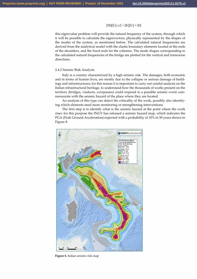
The first step is to identify what is the seismic hazard at the point where the work

rises: for this purpose the INGV has released a seismic hazard map, which indicates the

PGA (Peak Ground Acceleration) expected with a probability of 10% in 50 years shown in

Figure 8.

Figure 8. Italian seismic risk map



In 2008, the Technical Standards for Construction (NTC) [4] were introduced, which de-

fine the methods according to which these analyses must be performed.

First of all, nine return periods are identified, corresponding to 30, 50, 72, 101, 140, 201,

475, 975, 2475 years. A return period indicates the time in which, statistically, an event of

a certain magnitude may recur.

Three values are defined for each of these periods:

• ag (or PGA), maximum horizontal ground acceleration;

• F0, maximum value of the amplification factor of the spectrum in horizontal accel-

eration;

• T*C, start period of the constant velocity section of the spectrum in o-horizontal ac-

celeration.

These values describe the seismic spectrum, shown in figure 9, i.e. the time trend of

ground acceleration for that given return.

Figure 9. seismic spectrum

On the basis of the seismic spectrum, the accelerograms which will be used in the simu-

lation are generated numerically: these are artificial signals whose deviation must not

exceed 10% below and 30% above the starting spectrum [17-19].

The results obtained from the dynamic finite element analysis are then summarized in a

series of fragility curves associated with the work; these curves indicate the probability of

reaching a certain level of damage, which may represent light, moderate, severe or col-

lapse of the infrastructure [20-21].

2.5 OpenSees software

OpenSees (Open System for Earthquake Engineering Simulation) is a software

framework for simulating the seismic response of structural and geotechnical systems

using finite element simulation.

OpenSees is open-source, and was originally developed as a computational platform

for earthquake engineering research at the Pacific Earthquake Engineering Research

Center, a research program of Berkley University of California.

The framework has advanced capabilities for modeling and analysis of systems us-

ing a wide choice of models, elements, and resolution algorithms. It is also prepared for

parallel computing, thus ensuring scalability of simulations [25-28].

OpenSees uses object-oriented methodologies to offer maximum modularity and

extensibility, is written primarily in C++ with numerical libraries in Fortran and C.



Figure 10. logical schema of the OpenSees class hierachy

The executable is essentially an interpreter based on the TCL scripting language, which is

installed together with the framework, and the input files will then be written following

the rules of that language.

The execution of a simulation using OpenSees is divided into three basic steps:

1. Creation of the model

2. Analysis on the created model

3. Output of the analysis

2.5.1 Creation of the model

OpenSees provides beam-column elements and continuum elements to create

structural and geotechnical models. A wide variety of uniaxial materials and sections for

beam-column elements are also available.

The model creation process consists of generating one or more .xtcl files containing

information about the system. In particular, the nodes, materials, sections, elements

connecting the nodes, and masses to be applied to the nodes must be defined.

Figure 11. Representation of the OpenSees model

This information will be passed to the ModelBuilder module, which will take care of

generating a mathematical model of the system to be simulated.

2.5.2 Types of analysis

Nonlinear analysis requires a variety of algorithms and resolution methods. Open-

Sees provides both static and dynamic nonlinear methods, equation solvers and methods

for the management of constraints.



The dynamic analysis, performed for this project according to the indications of the

Technical Standards for Construction - NTC 2008, foresees the use of 9 return times, fixed

at 30, 50, 72, 101, 140, 201, 475, 975 and 2475 years, for each of which are extracted the

values ag, f0, T*c according to the local seismic hazard at the site of the work (see §2.4.1)

Starting from these 3 values, the so-called artificial signals are numerically created,

i.e. random accelerograms in the X (longitudinal with respect to the work) and Y (trans-

verse) coordinates which reproduce the pga (peak ground acceleration) typical of an

earthquake. Each accelerogram is defined for a minimum duration of 25 seconds, ac-

cording to NTC08 [4].

The analysis of the OpenSees software simulates the response of the infrastructure to

the seismic action, recording the forces applied to its various elements and the conse-

quent displacements.

2.5.3 Solving algorithms

The main incremental iterative procedures are available in OpenSees, for nonlinear

analysis. The available algorithms are Newton-Rapson, Newton-Rapson with inline

search, and Broyden and derivatives. The algorithms are used in the order presented,

later in case the convergence of the previous one fails [31-32].

• the Newton-Rapson algorithm is the most widely used and most robust iterative

method for re-solving systems of nonlinear algebraic equations. It is also the most

demanding in terms of computational effort because the stiffness matrix must be

updated at each iteration step.

• the Newton-Rapson algorithm with line search introduces line search to solve the

nonlinear residual equation. Line search increases the effectiveness of Newton's

method when convergence is slow due to the roughness of the residual. The stiffness

matrix is not updated at each step. This implies reduced computational effort, which

is the advantage of this method. The disadvantage of this method is that it requires

more iterations than Newton's method, so convergence is slower.

• Broyden's algorithm is for general non-symmetric systems. It performs successive

rank-one updates of the tangent at the first iteration of the time step. This algorithm

is only used in critical cases because the algorithm concentrates iterations at points

where the solution has difficulty converging, hence convergence is slower.

2.5.4 Analysis output

OpenSees allows to decide which quantities will have to be saved on file after the

execution of the simulation, through the Recorders. These are listed again in a file .xtcl, in

which some parameters are indicated, as for example on which element the Recorder will

have to act (Nodes or Elements), the output file in which to save the results, the type of

result to save (localForce, basicDeformation, etc.)

The output of the analysis can be found in 3 files with extension .out:

- recorderNodeDisplacements.out

- recorderEleLocalForces.out

- recorderEleBasicDeformation.out

For the purposes of the case study, the file that will be taken into account will be

recorderNodeDisplacements.out, in which there are 6 values for each node of the model:

the displacement in the 3 axes X, Y, Z, and its rotation, always in the 3 axes.

It is a textual file, where the first line indicates the initialization of the model and

re-ports a series of zeros, while the subsequent lines are the result of 25 seconds of sim-

ulation with steps of 0.01 seconds, for a total of 2500 lines.



3. Case Study: Visualization of Seismic Risk

The idea at the base of the experimental project is to visualize the results of the sim-

ulations carried out using the OpenSees software directly on a three-dimensional model

of the infrastructural work, through the use of color gradations to indicate the amplitude

of the stresses suffered.

To better place the work within the real environment in which it is located, it was

decided to add the three-dimensional model of the surrounding area, obtaining the

elevation from the DEM (Digital Elevation Model) on the INGV website, and the texture

from satellite maps.

3.1 Implementation approch

For the purposes of the project we focused on 8 works (bridges, viaducts, flyovers)

as examples of the Italian infrastructural heritage. Of these works the model for Open-

Sees has been created and the dynamic analyses have been performed as per NTC08

standards (see §2.4.1).

Table 1. Data of the analyzed works

Work name Model Coordinates

Viadotto La Tora I

15.7675, 40.6247

Ponte SS17

14.2581, 41.6013

Viadotto Irminio

14.7315, 36.8639

Ponte Sinarca

14.958, 42.00517

Ponte SS17

13.0813, 42.42227

Viadotto Tronto II

13.2639, 42.6895

Viadotto Pietrarossa

13.5903, 37.8249



Viadotto Vella

13.938, 42.04391

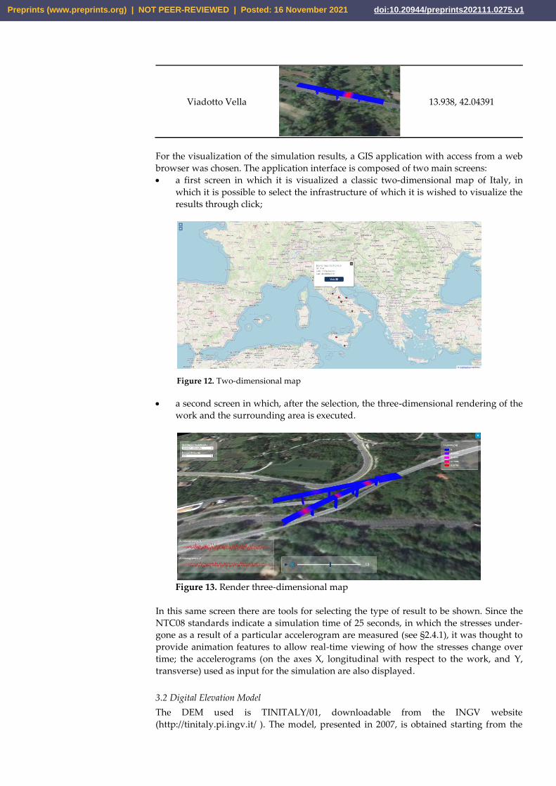
For the visualization of the simulation results, a GIS application with access from a web

browser was chosen. The application interface is composed of two main screens:

• a first screen in which it is visualized a classic two-dimensional map of Italy, in

which it is possible to select the infrastructure of which it is wished to visualize the

results through click;

Figure 12. Two-dimensional map

• a second screen in which, after the selection, the three-dimensional rendering of the

work and the surrounding area is executed.

Figure 13. Render three-dimensional map

In this same screen there are tools for selecting the type of result to be shown. Since the

NTC08 standards indicate a simulation time of 25 seconds, in which the stresses under-

gone as a result of a particular accelerogram are measured (see §2.4.1), it was thought to

provide animation features to allow real-time viewing of how the stresses change over

time; the accelerograms (on the axes X, longitudinal with respect to the work, and Y,

transverse) used as input for the simulation are also displayed.

3.2 Digital Elevation Model

The DEM used is TINITALY/01, downloadable from the INGV website

(http://tinitaly.pi.ingv.it/ ). The model, presented in 2007, is obtained starting from the



individual DEMs of the different Italian administrative regions, and has a resolution of 10

meters per pixel; it is available in GeoTIFF format, with UTM WGS84 projection, zone 32

[6].

Figure 14. Digital Elevation Model TINITALY/01

All the GeoTIFF related to the position of the works taken into consideration have been

downloaded from the INGV website. Since the downloaded tiles cover a very large area,

using QGIS software we proceeded to the cropping of the area of interest (area of 1km x

1km having as center the coordinates of the work). The file was then saved in ENVI

format, which presents the GeoTIFF data as a simple vector of binary data [7], ready to be

read by the Three.js graphic library used in the front-end for the assignment of elevation

to the three-dimensional mesh (see §3.7.2).

Each pixel is represented within the ENVI format by 4 bytes that make up a floating point

(floating point) value with 32 bits of precision. The order of the bytes is LSF (least signif-

icant first). The floating point format allows you to use the data directly in Three.js

without having to make any kind of conversion, simplifying the process and ensuring an

excellent resolution.

Again through QGIS, the extension of the layer obtained from the DEM was used to save

to file the corresponding portion of the satellite map of the area, which will later be used

as a texture to be applied to the ground mesh (see §3.7.3).

3.3 System architecture

The workflow of the project involves the use of an off-line component, to be exe-

cuted once when adding a new work, called "Conversion Tool". This component allows

the OpenSees output files to be adapted into the formats required by the application.



Once the necessary files are created, the web application follows the client-server

architecture, with a Java back-end and an HTML / CSS / javascript front-end published

via Tomcat application server.

Figure 15. System architecture

3.4 Conversion tool

The conversion tool is built in Java. It is located in the same project as the web applica-

tion, in a reserved package named "processing". The Processing Analysis class takes care

of reading some of the OpenSees output files and producing the files needed by the ap-

plication in .JSON format.

The first operation performed by the tool is the loading in memory of the data contained

in the files nodes.xtcl and elements.xtcl through the methods :

loadFileNodes(String filename)

loadFileElements(String filename)

The data of nodes and model elements are saved in data structures in memory, specifi-

cally HashMaps with the node/element id as key, using auxiliary classes Node and Ele-

ment:

public Map<Integer, Node> nodesList;

public Map<Integer, Element> elementsList;



Figure 16. OpenSees model visualization

Figure 16 shows the model generated for OpenSees analysis: the white dots represent the

nodes, and the green lines the elements that connect them.

OpenSees associates to each node of the model a section; the extrusion of this section will

then represent what will be displayed in the interface, and is saved in the

bridge_model.csv file; the next step is then to load the three-dimensional model in

memory, and associate to each face the reference node. In figure 17 you can see the same

model of figure 16 with the sections associated to each node.

Figure 17. OpenSees with the sections of each node

OpenSees saves data sequentially, so it is sufficient to cycle through all elements of the

bridge_model.csv file and its elementList elements to have a correct association.

All these operations are carried out from the method

loadFileModel(String filename)

After the model has been loaded in memory and saved in the .json file, it remains only to

create the files that will serve for the various thematizations. Inside two nested cycles that

take into consideration all the return times and the three required output types, the ac-

celerograms files are first read and saved in .json format, through the method

creaJsonAccel(String id, String tr, String simul, String dir)

subsequently it comes executed the methods

loadFileNodeDisplacements(String filename, String result)

creaJsonTematization(int t)



The first takes care of reading the file RecorderNodesDisplacement_[tr]-1 and extracting

the required re-sult, while the second will generate, from these results, a json structure in

which for each node are listed the RGB values appropriately scaled, and the minimum

and maximum values used to populate the legend.

All RecorderNodesDisplacement files are composed of sequences of [number of nodes] *

6 elements, where the 6 values indicate:

• X-axis displacement

• Y-axis displacement

• Z-axis displacement

• X-axis rotation

• Y-axis rotation

• Z axis rotation

For the purposes of the project are taken into account the first 3, since the rotations of the

elements are not very significant.

The file records the results on 25 seconds of simulated shock, with steps of 0.01 seconds,

for a total of 2500 rows; in order to keep the data structures manageable, it was decided to

sample the results every second, thus obtaining 25 data sets corresponding to the 25

seconds of simulation. The data sets are then saved in an array within the json structure.

The files obtained from the procedure can finally be copied into the WebCon-

tent/assets/[work id]/ folder of the project in order to be served to the front-end at the

time of the request.

3.5 Back-end

The back-end is realized in Java and executed through Tomcat application server. It

is based on the use of servlets, collected in the appropriate package “servlet” and recalled

by URL from the front-end. The necessary servlets are registered in the file Web-

Con-tent/WEB-INF/web.xml to allow the server to know their location and the URL to

which they must respond.

Given the simplicity of the system architecture, the back-end is composed of two

main servlets:

the first one is named GetFeatures and it takes care of reading from file system the

data related to the points of interest, organizing them in json format and passing them to

the front-end, where they will then be displayed as layers on a map. The file in which

these data are saved is in .CSV format and is called "opere_feat.csv". Its location on the

file system is configurable through the "config.conf" file.

The second is called GetDatiOpera and provides the front-end, at the time of selec-

tion of a work, all the data necessary for its visualization, and then:

• Latitude and longitude of the model;

• Orientation with respect to north and elevation of its lowest foundation;

• Latitude and longitude limits of the terrain mesh (Minimum and Maximum Lati-

tude, Minimum and Maximum Longitude);

• X and Y dimensions of the terrain mesh in meters.

These data are also saved in a .CSV file called "data_opere.csv" in the same folder on

file system as the previous file.

3.6 Front-end

The front-end uses some auxiliary libraries for geographic and three-dimensional

visualization. The libraries used are listed in table 2:



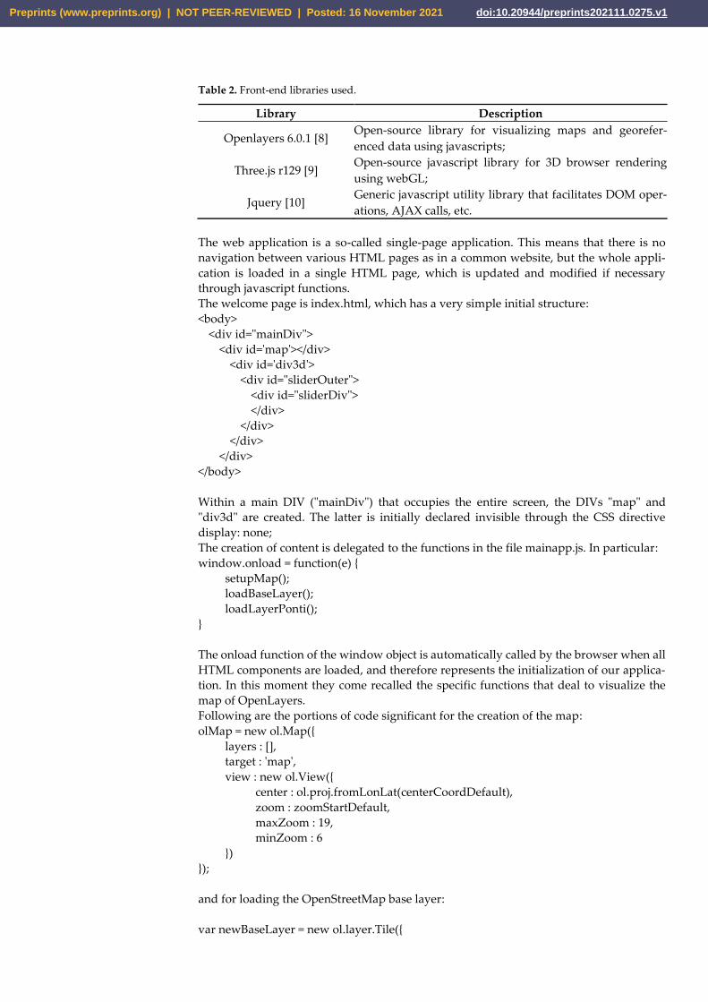
Table 2. Front-end libraries used.

Library Description

Openlayers 6.0.1 [8] Open-source library for visualizing maps and georefer-

enced data using javascripts;

Three.js r129 [9] Open-source javascript library for 3D browser rendering

using webGL;

Jquery [10] Generic javascript utility library that facilitates DOM oper-

ations, AJAX calls, etc.

The web application is a so-called single-page application. This means that there is no

navigation between various HTML pages as in a common website, but the whole appli-

cation is loaded in a single HTML page, which is updated and modified if necessary

through javascript functions.

The welcome page is index.html, which has a very simple initial structure:

<body>

<div id="mainDiv">

<div id='map'></div>

<div id='div3d'>

<div id="sliderOuter">

<div id="sliderDiv">

</div>

</div>

</div>

</div>

</body>

Within a main DIV ("mainDiv") that occupies the entire screen, the DIVs "map" and

"div3d" are created. The latter is initially declared invisible through the CSS directive

display: none;

The creation of content is delegated to the functions in the file mainapp.js. In particular:

window.onload = function(e) {

setupMap();

loadBaseLayer();

loadLayerPonti();

}

The onload function of the window object is automatically called by the browser when all

HTML components are loaded, and therefore represents the initialization of our applica-

tion. In this moment they come recalled the specific functions that deal to visualize the

map of OpenLayers.

Following are the portions of code significant for the creation of the map:

olMap = new ol.Map({

layers : [],

target : 'map',

view : new ol.View({

center : ol.proj.fromLonLat(centerCoordDefault),

zoom : zoomStartDefault,

maxZoom : 19,

minZoom : 6

})

});

and for loading the OpenStreetMap base layer:

var newBaseLayer = new ol.layer.Tile({



source : new ol.source.OSM({

url : "https://tile.openstreetmap.org/{z}/{x}/{y}.png",

crossOrigin : null

}),

id : 'base_layer',

name : "Base Map"

});

olMap.addLayer(newBaseLayer);

Always using the Openlayers functions, the click selection functionality has been added

to the map, which will allow to open the pop-up window.

The 3D visualization is realized using the Three.js library. Starting with version r106, the

recommended method of using this library is using modules defined by ECMAscript

version 6, often called ES6 modules [13-15]. This modular architecture has been created to

insert also in javascript the concept of "class" already present in other languages like C++

and Java, to allow to import in the project only the required functionalities of a given li-

brary, and to limit the scope of the variables reducing the risk of overlapping typical of

the use of global variables, and the elasticity of the Javascript language that does not

signal as an error the multiple declaration of the same variable.

The concept of an ES6 module is that everything that is declared inside it is not visible to

the outside, apart from the methods that are explicitly exported through the instruction

export {function};

From the outside, I can import the necessary functions of the module via the directive:

import {

funzione

} from './modulo.js';

In the project, it is therefore present the specially created module page3D.js that exports a

single function, render3Dview, which in turn imports the three.js library and performs

the rendering of the three-dimensional scene.

The basic operations performed by render3Dview are:

• Initialization of Three.js and creation of the scene

• Loading of all the necessary files (3D model, Digital Elevation Model, textures,

tematizations)

• Creation of the elements of the interface

• Render of the scene

To facilitate the generation of the elements of the interface have been created two custom

components that exploit the potential of HTML5 canvas:

• slider.js : this is a component that shows two buttons (Play and Stop) and a time

slider bar with a slider. When Play is pressed, it creates a setInterval function that

executes a callback function specified by the user at each predefined interval; at the

same time it advances the slider on the scroll bar, thus creating a real-time anima-

tion;

• acceler_graph.js : draws a graph from an array of data, scaling the vi-sualized data

based on the height of the DIV in which it was inserted. It allows the setting of a

vertical bar, thus realizing the synchrony with the position of the animation slider.

3.7 Trhree-dimensional rendering

The Three.js library provides all the necessary tools to create a 3D scene complete

with three-dimensional objects, lights, cameras and effects within a normal web page.

In figure 18 it is represented the conceptual diagram of a Three.js scene.



Figure 18. Diagram of a three.js scene

The Renderer is the object that takes care of representing on screen all that is present in a

Scene, as if the user were positioned in the point where the Camera is present, that is a

real camera with a position, an orientation and a Field of View that frames the scene.

Inside the Scene we find all the objects that make up the "set" that we are going to frame:

the Mesh are the real 3D objects, which in turn are composed of Geometry, the polygonal

geometries that describe its appearance, and Material, the materials that define color,

light reflection properties, etc. The materials can refer to textures, raster decals that are

applied to the geometries.

As mentioned, on the screen will be displayed what the camera is framing, within the

so-called "frustum", a truncated pyramid-shaped area bounded by the Field of View of

the camera (fov) and the clipping planes near and far. A representation of the frustum is

visible in Figure 19.

Figure 19. Representation of “frustum”

A great importance in any three-dimensional space is the coordinate system: although

they are always composed of the three axes X, Y, Z, in some cases we consider the Z as

the vertical axis, in others the Y. Three.js uses the latter convention, as shown in Figure

20.



Figure 20. Coordinate system of Three.js [12]

Since in geographic systems the values of longitude and latitude are often reported to X

and Y coordinates, it would be more convenient to use a reference system in which the Z

axis corresponds to the elevation, then the vertical axis; fortunately the library allows you

to change the reference system through a single function:

THREE.Object3D.DefaultUp = new THREE.Vector3(0, 0, 1);

This function creates a unit vector in the Z-direction and assigns it to the one that is con-

sidered "high" (Up); in this way you have returned to the desired condition.

3.7.1 Polygonal Rendering

At the base of the rendering techniques used by three.js is polygonal rendering. This

technique consists in approximating any object that is represented in a three-dimensional

space to a series of polygons, and in particular everything is represented by triangles,

called faces, as visible in figure 21.

Figure 21. Polygonal mesh

The order in which the three vertices of the triangle are listed is very important, as they

define whether it faces the Camera or the other direction; in particular, three.js uses a

counterclockwise convention, as shown in Figure 22.



Figure 22. Orientation of a triangle

A very important quantity that must be calculated for each triangle is its normal. This is a

unit vector perpendicular to the plane formed by the vertices of the triangle that will al-

low, compared to the angle of incidence of the light source (or sources in the case of

multiple illumination) to determine the degree of illumination of that face.

In the example of figure 23, N1, N2, N3 and N4 are the normals of the four faces that

make up the mesh.

Figure 23. Normals on a 4-sided mesh

In the most recent rendering engines, this value is interpolated for each point of the face

taking into account the normals of neighboring faces; this technique, which takes the

name of Gouraud Shading, allows you to generate more harmonious shapes and not

"faceted" as those obtained with a flat lighting for each face (Flat Shading).

In the Three.js library, the first step in creating a polygonal mesh is to define its geometry.

For this purpose you can use the THREE.BufferGeometry object that replaces the previ-

ous THREE.Geometry for performance reasons. A BufferGeometry is in fact represented

by one-dimensional arrays in which the X, Y, Z coordinates of each point are listed below,

without objects containing them. This approach, although less intuitive for the developer,

allows the webGL libraries a significant performance boost.

In the case where many vertices are shared among several faces, as is often the case, you

can list them once in the position array and then create a second index array that simply

lists references to the vertices of each face.

Once the two arrays are filled with the model data, it is possible to associate them with

the Buffer-Geometry through the instruction:

geometry.setAttribute('position', new THREE.Float32BufferAttribute(vertices, 3));

geometry.setIndex( indices );

in which it comes created an appropriate object of Three.js, Float32BufferAttribute, be-

ginning from the vector, and this comes then assigned to the attribute "position" of the

BufferGeometry.



The array of indices is instead directly set via the setIndex function. The coloration of the

model in this plan is dependent from a sure value assumed from the vertices (tied up to

the nodes of the simulation, v. 4.3.1). It is therefore chosen to use, rather than textures

applied to the model, a technique called Vertex Shading, that allows to assign a color to

every vertex of the figure. The rendering engine will then interpolate the colors

throughout the surface of the face, as visible in Figure 24.

Figure 24. example of vertex shading

This is possible by setting the vertexColors attribute to true in the material:

const material = new THREE.MeshPhongMaterial({ ambient: 0x050505, vertexColors:

true, specular: 0x5555, shininess: 0 });

and then setting a new attribute ("color") of the geometry, passing an array containing the

R, G, B components normalized between 0.0 and 1.0 of each vertex.

geometry.setAttribute('color', new THREE.Float32BufferAttribute(colors, 3));

3.7.2 Elevation assignment

The mesh representing the portion of land surrounding the work is a simple plane

geometry:

const geometry = new THREE.PlaneGeometry(1000, 1000, 99, 99);

Since the real dimensions of the area are 1000x1000 meters, it is convenient to gen-

erate the mesh of the same dimensions (parameters 1 and 2). The third and fourth pa-

rameters represent the number of subdivisions that the plane must have on the X and Y

axes.

Dividing the geometry into 99 sections per side, we will find ourselves with exactly

100 vertices, a number equal to the values we extracted from the DEM.

At this point, after having read the values of the ENVI file that was previously saved

in the /assets folder (see §3.4), it will be sufficient to save them in an array of type

Float32Array and overwrite the Z value of the array "position" of the geometry to include

the elevation data in the terrain model.



Figure 25. Terrain mesh before and after applying elevation

3.7.3 Terrain Texture

The texture to be applied to the terrain mesh was obtained through QGIS. The

pro-gram allows in fact to add a layer "XYZ Tiles" that accepts custom connections. It will

be sufficient to choose a service that offers satellite maps; at this point, through the tool

"Convert map to raster", you can save the desired portion of the map as GeoTIFF on file

system. The extension will be given by the layer that has been previously cropped from

the DEM; a tile size of 1000 will be chosen, equal to the meters of the area of interest, and

a "Map unit per pixel" equal to 1. In this way we will have 1 pixel for each meter of land,

which guarantees a good quality of texture without too high resolutions that would

compromise the performance of the application.

The GeoTIFF format is a lossless format, so there is no quality loss due to compres-

sion, but unfortunately it generates large files. Fortunately GeoTIFF is read by graphics

programs as if it were a normal TIFF. This was then converted to JPEG format, which is

web-friendly and greatly reduces the size of the generated file.

The result of the conversion was then copied like the other files in the assets/ folder

and imported into three.js using the instructions:

const loader = new THREE.TextureLoader();

loader.crossOrigin = "";

const textureTerreno = loader.load(file, callback)

Next, the texture can be assigned to a new material that, associated with the previously

generated geometry, will form the mesh of the terrain (see figure 26).

Figure 26. Terrain mesh before and after applying elevation



3.7.4 Positioning the model of the work

Once the terrain mesh has been created and inserted into the scene, the

three-dimensional model of the work must be positioned, applying the correct X, Y, Z

coordinates and rotation so that it is correctly inserted with respect to the surrounding

terrain. Such operations are performed by the function posizionaPonte() of the page3D.js

file, of which it is brought back the meaningful portion:

var diffLon = endLon - startLon;

var diffLat = endLat - startLat;

var x = ((lon - startLon) * dimTerrenoX) / diffLon - (dimTerrenoX / 2.0);

var y = ((lat - startLat) * dimTerrenoY) / diffLat - (dimTerrenoY / 2.0);

for (var i = 0; i < bridge.length; i++) {

var mesh = bridge[i];

mesh.position.x = x;

mesh.position.y = y;

mesh.position.z = elev - baseZ;

mesh.rotation.set(0,0,degrees_to_radians(rotaz));

}

The first operation performed is the calculation of the dimensions in WGS84 degrees of

the terrain mesh (variables diffLon and diffLat). Using these values, the initial coordi-

nates of the terrain, the coordinates of the bridge and the size in meters of the terrain,

through a simple proportion we obtain the X and Y coordinates of the three-dimensional

space in which to place the model.

Since the model is composed of various meshes saved in the bridge array, click on the

elements of the bridge array applying to each one the translation through the

mesh.position object. For the Z coordinate the elevation of the work is used (elev varia-

ble, normalized with respect to the minimum elevation of the baseZ terrain).

The instruction mesh.rotation.set(x, y, z) allows you to set the rotation angle of a mesh

and is used with the value of rotation of the work with respect to north, appropriately

transformed in radians from its initial value in degrees.

4. User Interface

The user interface is presented with a main screen where it is possible to select from

the map the work of which it is interesting to know the data. After the selection, a second

full-screen will open in which the work will be rendered.

4.1 Two-dimensional visualization

The initial screen shown when the web page is loaded is dominated by the

two-dimensional map centered on Italy. On the top left are the zoom adjustment keys,

and all the mouse commands are active: panning by moving the cursor while pressing

the left key, zoom in/out by the central wheel. The outward zoom is limited in order to

keep the user's attention on the area of interest.



Figure 27. Two-dimensional display screen

The base map displayed is that of OpenStreetMap [15]. Above it there is a layer with

point elements, represented by red circles; this layer represents the works of which

seismic verifications have been performed using OpenSees.

It is possible to click on one of the points of interest to show a pop-up window containing

the basic information of the work: its name, the internal id of the application, its coordi-

nates in the form of Longitude and Latitude WGS84.

The pop-up can be closed with the "X" button at the top right of the window.

In addition to the summary data of the work, the pop-up also contains the "3D View"

button. Pressing the button will take you to the 3D view of the artwork.

4.2 Three-dimensional visualization

Once a work is selected, the main view of the application opens: the 3D render. Once

all the necessary files have been loaded (bridge model, thematic, elevation model, terrain

textures), the screen will appear as shown in figure 28:

Figure 28. Three-dimensional display screen

The main components of the interface are:

1. Three-dimensional model of the work

2. Ground Mesh

3. Selection menu of the quantities to show

4. Accelerograms

5. Animation toolbar

6. Legend



Navigation within the three-dimensional screen can be performed by mouse and key-

board controls: by moving the cursor while pressing the left key it is possible to rotate the

view around the model; by using the central wheel it is possible to zoom in/out; by

pressing the SHIFT key while dragging the mouse it is possible to pan the camera to

move within the scene.

Through the selection menu (3) it is possible to select:

a) The simulated size to show on the model. The 3 possible choices are:

• X axis displacement. It represents the displacement of the nodes of the model in

longitudinal direction with respect to the work.

• Y axis displacement. It represents the displacement of the nodes of the model in

transverse direction with respect to the work.

• Displacement (module). It represents the modulus of the vector resulting from the

two X and Y displacements. It indicates the generic stress borne by the node, re-

gardless of its direction.

b) The time of return to show on the model. In this case the possible choices are 9: 30

years, 50 years, 72 years, 101 years, 140 years, 201 years, 475 years, 975 years, 2475 years.

At each change of selection, the data set for the model is reloaded for all 25 seconds that

make up the simulation; also the legend is repopulated to reflect the new minimum and

maximum limits of the data set taken into account.

In case of change of the return time, also the accelerograms are redrawn as these are de-

pendent on the selected return time.

Through the toolbar of animation is possible to move among the various instants of the

simulation, with steps of one second each. The operation is intuitive and resumes that

one of any player video.

Figure 29. toolbar animation

The animation can be scrolled in two ways: an automatic mode, activated by the "Play"

button, which will scroll the moments in real time. This mode can be stopped by pressing

the "Stop" button.

The second mode is manual: in this case you just need to drag the slider on the time bar to

move as you like along the 25 seconds.

On the right of the bar there is a number that indicates the frame (in seconds) displayed at

that moment.

At each change of time the coloration of the model is automatically updated, allowing to

evaluate which are the points of the work more stressed by the seismic shock. The color

gradations can be easily compared with those present in the legend, to have also a nu-

merical indication of the entity of the displacement.



Figure 30. Differences in coloration in different frames

The accelerogram graphs have a vertical bar, which automatically moves to follow that of

the animation: in this way it is also possible to compare the response of the elements in

relation to the input data used by OpenSees at that time.

At any time you can press the "X" button at the top right of the screen to return to the

two-dimensional view and select a new work.

5. Conclusions and future work

5.1 Conclusions

The project has shown how a rapid visual representation of the numerical results

can improve the understanding of the most stressed areas of an infra-structural work

subject to seismic movements.

It has also allowed to appreciate the difference in behavior between works of dif-

ferent types, in particular in the presence of very high piers or particularly long decks.

The platform can be used in particular when it is necessary to divulge the results

obtained from analyses carried out on the works, thus allowing even those who do not

have specific skills to evaluate qualitatively the effects on the stressed structures, com-

paring these effects on the basis of different PGA, and therefore of different intensity of

the earthquake.

The choice of the direction in which to visualize the displacements, on the longitu-

dinal or vertical axis of the bridge, allows to highlight how the horizontal elements such

as decks undergo vertical displacements, while the vertical elements (piers) have on the

contrary a longitudinal displacement with respect to the development of the work.

The modularity with which the architecture of the system has been designed makes

it easy to add new works of which the analyses carried out using the OpenSees software

are available: the conversion tool takes care of adapting the format of the output files and

performing the calculations necessary to display the results, while the saving of the data

of the works on .CSV files guarantees maximum ease in adding new points of interest to

the platform.



The product, although designed to show the results of a seismic analysis, can be

easily adapted to display any type of stress to which a structure is subjected: for example,

again for bridges, it would be possible to perform FEM analysis on the vertical loads to

which the decks are subjected; or one could focus on other infrastructural works such as

buildings, retaining walls or tunnels.

The development of this platform has also highlighted how nowadays it is possible

to obtain professional results even using o-pen-source software and libraries, and there-

fore free of charge, thus allowing even small companies to create tools that can be used

by professionals to evaluate and disseminate the results of their numerical analysis.

The major difficulties encountered in the creation of the application were certainly in

finding and interpreting the data of the analysis, a part certainly more the competence of

professionals in the field of structural engineering.

5.2 Future work

The project, at present, requires a series of operations for the addition of new works:

in addition to the results of finite element analysis, a basic element to be able to thematize

the model, there are several steps to follow, mostly through a special software such as

QGIS, to create the elevation files derived from the DEM and the textures to be applied to

the terrain model.

An evolution of the platform could, starting from the coordinates of the work to be

added, query directly the INGV site to download the portion of DEM desired and obtain

from this the area of 1km x 1km around the work; in the same way, satellite images of the

area could be obtained through the WMS service and saved on the file system, or loaded

into the browser at each request.

These operations, addressed to a user with administrator privileges, could be col-

lected in a web editor, together with other operations for fine-tuning the positioning of

the work, such as the possibility of modifying the coordinates, the elevation, the rotation

with respect to the north, to ensure that the model is correctly positioned on the ground

mesh.

Regarding the types of data displayed on the model, in addition to the displacement

values currently displayed, OpenSees also makes available the values related to the

forces to which the elements of the work are subjected, which could constitute additional

values that can be displayed through color gradations.

A further development could also show, since the displacements of each node in the

three directions X, Y, Z are available, the real-time animation with the actual displace-

ment of the vertices of the three-dimensional model, relatively to the values of the ref-

erence node.

As for the three-dimensional model, at the moment it is a simplified model gener-

ated from nodes, extruding the sections associated with them, for a more accurate rep-

resentation the ideal would be to have access to the more detailed model that OpenSees

creates within it to perform the analysis, this would involve, however, in addition to re-

search on the actual possibility of exporting this model, also an operation of optimization

of the mesh to make it viewable on the browser without overloading the graphics hard-

ware of the computer that runs it.

Author Contributions: Conceptualization, M.M.; methodology, M.M.; software, D.Q.; validation,

M.M., D.Q.; formal analysis, M.M.; data curation, M.M. and D.Q.; writing—review and editing,

M.M. and D.Q.; supervision, M.M.

Funding: This research received no external funding.

Data Availability Statement: The source of the data of the seismic maps are the INGV Institute

(National Institute of Geophysics and Volcanology) that since 2004 releases this map of seismic

hazard with which it provides a picture of the most dangerous areas in Italy.

(http://zonesismiche.mi.ingv.it).



Acknowledgments: The authors thank Pacific Earthquake Engineering Research Center as a source

of documentation necessary for the conduct of this paper.

Conflicts of Interest: The authors declare no conflict of interest.

References

1. QGIS project, QGIS documentation – Coordinate Reference System, https://docs.qgis.org/3.16/en/docs/ (accessed on

25/06/2021)

2. Metaingegneria.com, https://www.metaingegneria.com/cos-e-una-simulazione-fea/ (accessed on 25/06/2021)

3. INGV Terremoti, https://ingvterremoti.com/la-pericolosita-sismica/ (accessed on 25/06/2021)

4. D.M. 14 gennaio 2008, Approvazione delle nuove norme tecniche per le costruzioni

https://www.camera.it/cartellecomuni/leg15/RapportoAttivitaCommissioni/commissioni/allegati/08/08_all_dm_2008.pdf

(accessed on 25/06/2021)

5. OpenSees user documentation, https://opensees.berkeley.edu/wiki/index.php (accessed on 25/06/2021)

6. Tarquini S., Isola I., Favalli M., Battistini A. (2007) TINITALY, a digital elevation model of Italy with a 10 meters cell size (Ver-

sion 1.0) [Data set]. Istituto Nazionale di Geofisica e Vulcanologia (INGV). https://doi.org/10.13127/TINITALY/1.0.

7. L3Harris Geospatial, https://www.l3harrisgeospatial.com/docs/enviimagefiles.html ENVI image Files (accessed on 25/06/2021)

8. Openlayers API, https://openlayers.org/en/latest/apidoc/ (accessed on 25/06/2021)

9. Threejs.org documentation, Getting Started, https://threejs.org/docs/index.html#manual/en/introduction/Creating-a-scene

(accessed on 25/06/2021)

10. Jquery.org, About, https://learn.jquery.com/about-jquery/ (accessed on 25/06/2021)

11. Mozilla Foundation - MDN Web Docs, JavaScript modules,

https://developer.mozilla.org/en-US/docs/Web/JavaScript/Guide/Modules (accessed on 25/06/2021)

12. Three.js Fundamentals, https://threejsfundamentals.org/threejs/lessons/threejs-fundamentals.html , Getting Started (accessed

on 25/06/2021)

13. Eric Lengyel, Mathematics for 3D Game Programming and Computer Graphics Third Edition, Course Technology 2012, pp.

175, 176

14. LearnopenGL.com, https://learnopengl.com/Getting-started/Shaders (accessed on 25/06/2021)

15. OpenStreetMap, https://www.openstreetmap.org/ (accessed on 25/06/2021)

16. Gomarasca Mario A., Elementi di geomatica, ASITA, 2004

17. Aviram A., Mackie K., Stojadinovic B., Guidelines for Nonlinear Analysis of Bridge Structures in California, 2008, Technical

Report 2008/03, Pacific Earthquake Engineering Research Center, University of California, Berkeley

18. Casarotti C., Pinho R., An adaptive capacity spectrum method for assessment of bridges subjected to earthquake action, 2007,

Bulletin of Earthquake Engineering, Springer, 377–390

19. ATC 40, 1996, Seismic evaluation and retrofit of concrete buildings, Volume 1

20. FEMA 273, 1997, NEHRP Guidelines for the Seismic Rehabilitation of Buildings

21. Caltrans SDC 2010, Caltrans Seismic Design Criteria version 1.6, California Department of Transportation, Sacramento, Cali-

fornia

22. Next Generation Attenuation Database, PEER Ground motion database,

http://peer.berkeley.edu/peer_ground_motion_database

23. Coleman J., Spacone E., Localization issues in force-based frame elements, 2001, Journal of Structural Engineering, Vol. 127

24. Priestley M. J. N., Seible F., Calvi G.M., Seismic Design and Retrofit of Bridges, 1996, Wiley, New York

25. Spacone E., Filippou F.C., Taucer F.F., Fibre beam-column model for nonlinear analysis of R/C frames: Part I. Formulation,

1996, Earthquake engineering and Structural dynamics, Vol. 25, 711-725

26. California Department of Transportation Division of Maintenance, Structure Maintenance and Investigations, BIRIS, Jambo-

ree Road Overcrossing

27. Aviram, A., Mackie, K.R., and Stojadinovic, B. (2008a). "Effect of abutment modeling on the seismic response of bridge struc-

tures." Earthquake Engineering and Engineering Vibration, 7(4), 395-402.

28. Aviram, A., Mackie, K.R., and Stojadinovic, B. (2008b). "Guidelines for nonlinear analysis of bridge structures in California."

PEER Report No. 2008/03, Pacific Earthquake Engineering Research Center, University of California, Berkeley.

29. Mazzei, M.; Palma, A.L. Analysis of Localization and Space Interaction Models. Proposal of very good linked model applied to

a study area for the localization of a large shopping mall. GEOMEDIA 2014, 18 (Suppl. 1), 265–275.

30. Mazzei, M.; Palma, A.L. Spatial Statistical Models for the Evaluation of the Landscape. In Computational Science and Its Applica-

tions—ICCSA 2013. ICCSA 2013. Lecture Notes in Computer Science; Murgante, B.; et al. Eds.; Springer: Berlin/Heidelberg, Ger-

many, 2014; Volume 7974, doi:10.1007/978-3-642-39649-6_30.

31. Mazzei, M.; Palma, A.L. Comparative Analysis of Models of Location and Spatial Interaction. In Computational Science and Its

Applications—ICCSA 2014. ICCSA 2014. Lecture Notes in Computer Science; Murgante, B.; et al. Eds.; Springer: Cham, Switzerland,

2014; Volume 8582, doi:10.1007/978-3-319-09147-1_19.

32. Mazzei, M. An Unsupervised Machine Learning Approach in Remote Sensing Data. In Computational Science and Its Applica-

tions—ICCSA 2019. ICCSA 2019. Lecture Notes in Computer Science; Murgante, B.; et al. Eds.; Springer: Cham, Switzerland, 2019,

doi:10.1007/978-3-030-24302-9_31.



33. Mazzei, M. Software development for unsupervised approach to identification of a multi temporal spatial analysis model. In Pro-

ceedings of the 2018 International Conference on Image Processing, Computer Vision, and Pattern Recognition, IPCV 2018, July 30

– August 02 Las Vegas, Nevada – USA CSCE’18 pp. 85–91, https://csce.ucmss.com/cr/books/2018/LFS/CSREA2018/IPC3126.pdf

34. Mazzei, M. An Unsupervised Machine Learning Approach for Medical Image Analysis. In Advances in Information and Com-

munication. FICC 2021. Advances in Intelligent Systems and Computing; Arai, K., Ed.; Springer: Cham, Switzerland, 2021; Volume

1364, doi:10.1007/978-3-030-73103-8_58.

35. Mazzei, M.; Di Guida, S. Spatial data warehouse and spatial OLAP in indoor/outdoor cultural environments. In Computer Sci-

ence (Including Subseries Lecture Notes in Artificial Intelligence and Lecture Notes in Bioinformatics); Springer: Cham, Switzerland,

2018, doi:10.1007/978-3-319-95168-3_16.

36. Mazzei, M.; Palma, A.L. Spatial multicriteria analysis approach for evaluation of mobility demand in urban areas. In Computer

Science (Including Subseries Lecture Notes in Artificial Intelligence and Lecture Notes in Bioinformatics) Book; Springer: Cham, Swit-

zerland, 2017, doi:10.1007/978-3-319-62401-3_33.



Documents

Article Development of a 3D webGIS application for the