Embed Size (px)
Citation preview
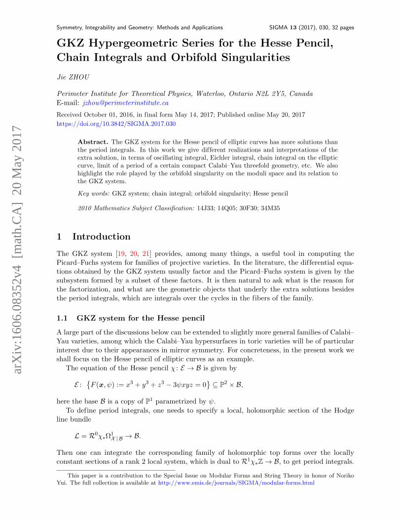
Symmetry, Integrability and Geometry: Methods and Applications SIGMA 13 (2017), 030, 32 pages
GKZ Hypergeometric Series for the Hesse Pencil,
Chain Integrals and Orbifold Singularities
Jie ZHOU
Perimeter Institute for Theoretical Physics, Waterloo, Ontario N2L 2Y5, Canada
E-mail: [email protected]
Received October 01, 2016, in final form May 14, 2017; Published online May 20, 2017
https://doi.org/10.3842/SIGMA.2017.030
Abstract. The GKZ system for the Hesse pencil of elliptic curves has more solutions thanthe period integrals. In this work we give different realizations and interpretations of theextra solution, in terms of oscillating integral, Eichler integral, chain integral on the ellipticcurve, limit of a period of a certain compact Calabi–Yau threefold geometry, etc. We alsohighlight the role played by the orbifold singularity on the moduli space and its relation tothe GKZ system.
Key words: GKZ system; chain integral; orbifold singularity; Hesse pencil
2010 Mathematics Subject Classification: 14J33; 14Q05; 30F30; 34M35
1 Introduction
The GKZ system [19, 20, 21] provides, among many things, a useful tool in computing thePicard–Fuchs system for families of projective varieties. In the literature, the differential equa-tions obtained by the GKZ system usually factor and the Picard–Fuchs system is given by thesubsystem formed by a subset of these factors. It is then natural to ask what is the reason forthe factorization, and what are the geometric objects that underly the extra solutions besidesthe period integrals, which are integrals over the cycles in the fibers of the family.
1.1 GKZ system for the Hesse pencil
A large part of the discussions below can be extended to slightly more general families of Calabi–Yau varieties, among which the Calabi–Yau hypersurfaces in toric varieties will be of particularinterest due to their appearances in mirror symmetry. For concreteness, in the present work weshall focus on the Hesse pencil of elliptic curves as an example.
The equation of the Hesse pencil χ : E → B is given by
E :F (x, ψ) := x3 + y3 + z3 − 3ψxyz = 0
⊆ P2 × B,
here the base B is a copy of P1 parametrized by ψ.
To define period integrals, one needs to specify a local, holomorphic section of the Hodgeline bundle
L = R0χ∗Ω1X |B → B.
Then one can integrate the corresponding family of holomorphic top forms over the locallyconstant sections of a rank 2 local system, which is dual to R1χ∗Z→ B, to get period integrals.
This paper is a contribution to the Special Issue on Modular Forms and String Theory in honor of NorikoYui. The full collection is available at http://www.emis.de/journals/SIGMA/modular-forms.html
arX
iv:1
606.
0835
2v4
[m
ath.
CA
] 2
0 M
ay 2
017
2 J. Zhou
A canonical choice for the local section is given by
Ω(ψ) = Resψµ0
F (x, ψ), µ0 := zdx ∧ dy + xdy ∧ dz + ydz ∧ dx. (1.1)
On each fiber Eψ of the family χ, the 2-form µ0/F gives a meromorphic 2-form on the ambientspace P2 with a pole of order one along Eψ and its residue gives a holomorphic top form onthis elliptic curve fiber Eψ. The integrals of this choice of holomorphic section, over a furtherchoice of the locally constant sections A,B of the above-mentioned rank 2 local system, givesthe period integrals
πA(ψ) =
∫A
Ω(ψ), πB(ψ) =
∫B
Ω(ψ).
The Picard–Fuchs equation can be derived, for example, by computing the Gauss–Maninconnection or by using the Griffiths–Dwork method. With respect to the choice Ω given above,the differential operator annihilating the period integrals is given by
LPF = (θψ − 2)(θψ − 1)− ψ3θ2ψ, θψ := ψ∂
∂ψ. (1.2)
Henceforward we shall frequently use the θ-operator defined as above.The details of the derivation for the GKZ system will be useful later in this work, so we recall
them here following [19].We first extend the family a little by rewriting the equation for (the total space) of the family
as
F (x,a) := a1x3 + a2y
3 + a3z3 + a0xyz = 0.
Then, one considers the actions on the polynomial F (x,a) which belong to the diagonalscalings inside the group GLx ×GLa and hence preserve the fibration structure. Here by GLx
we mean the affine transformations on C3 parametrized by x = x, y, z space and similarlyfor GLa. Those which fixes F up to an overall scaling forms a subgroup G. By construction,for any element in G, the scaling on a is determined by that on x. We can then choose thegenerators of G to be
(x1, x2, x3; a1, a2, a3, a0) 7→(λx1, x2, x3;λ
−3a1, a2, a3, λ−1a0
), λ ∈ C∗,
(x1, x2, x3; a1, a2, a3, a0) 7→(x1, λx2, x3; a1, λ
−3a2, a3, λ−1a0
), λ ∈ C∗,
(x1, x2, x3; a1, a2, a3, a0) 7→(x1, x2, λx3; a1, a2, λ
−3a3, λ−1a0
), λ ∈ C∗,
(x1, x2, x3; a1, a2, a3, a0) 7→(x1, x2, x3;λa1, λa2, λa3, λa0
), λ ∈ C∗. (1.3)
The former three also scale the meromorphic 2-form µ0 by λ, while the latter acts trivially.Hence when acting on the 2-form
ω(a) :=µ0
F (x,a), (1.4)
the infinitesimal versions of these group transformations give rise to the following annihilatingdifferential operators called Euler homogeneity operators,
Zi = θxi − 3θai − θa0 − degxi µ0, i = 1, 2, 3,
Z0 =3∑i=1
θai + θa0 − (−1).
GKZ Hypergeometric Series for the Hesse Pencil 3
Here degxi µ0 stands for the weight of µ0 under the action xi 7→ λxi, which is one in the currentcase.
Now the monomials in the pencil parametrized by ai, i = 0, 1, 2, 3 satisfy the relation
x31 · x32 · x33 = (x1x2x3)3.
This then gives the following differential operator that annihilates ω(a)
DGKZ =
3∏i=1
∂ai − ∂3a0 .
The projection1, which we denoted by χ∗, of the above differential operators to be basedirection yields
(χ∗Zi)ω = 0, i = 0, 1, 2, 3, (χ∗DGKZ)ω = 0.
One then translates these differential equations to the ones satisfied by the period integralsπγ(a) =
∫γ Ω with respect to the holomorphic top forms Ω = a0ω(
3θai + θa0 + degxi −1)
Ω = 0, i = 1, 2, 3,(3∑i=1
θai + θa0
)Ω,(
1∏ai
∏θai −
1
a30(θa0 − 3)(θa0 − 2)(θa0 − 1)
)Ω = 0. (1.5)
In the present case, degxi µ0 = 1, i = 1, 2, 3. The former two equations allow one to make theansatz
πγ(a) = πγ(z), z = −a1a2a3a30
. (1.6)
Now when acting on a function of z, the last differential equation gives
DGKZ πγ =(θ3z + z(−3θz − 3)(−3θz − 2)(−3θz − 1)
)πγ = 0. (1.7)
Specializing to a1 = a2 = a3 = 1, a0 = −3ψ, by disregarding the overall constants which areirrelevant throughout the discussions, we can see that (recall (1.2))
DGKZ =(θ3ψ − ψ−3(θψ − 3)(θψ − 2)(θψ − 1)
)= θψ
(θ2ψ − ψ−3(θψ − 2)(θψ − 1)
)= θψ ψ−3 LPF. (1.8)
When writing the Picard–Fuchs operator in terms of the α = ψ−3 coordinate, we use thefollowing normalization of the leading coefficient
LPF =
(θ2α − α
(θα +
1
3
)(θα +
2
3
)), (1.9)
so that up to a constant multiple we have DGKZ = θα LPF.We remark that for families of hypersurface Calabi–Yau varieties in toric varieties in any
dimension, similar discussions apply. In particular, one always obtains LPF from the factor inthe rightmost as in (1.8).
1A more intrinsic description can be given by the D-module language.
4 J. Zhou
1.2 Calabi–Yau condition and factorization of differential operator
By examining the derivation, a few observations are in order. First, the first equation in (1.5)is consistent with the second if and only if the following condition holds
3∑i=1
degxi µ0 = degF. (1.10)
We call this the Calabi–Yau condition since the meromorphic form µ0 is a section ofOP2(−(2+1))and the degree of the polynomial F matches with the degree of µ0 exactly when F = 0 definesa Calabi–Yau hypersurface in the projective space P2.
Now instead of making the ansatz mentioned before in (1.6), one can eliminate the differentialoperators θai , i = 1, 2, 3 by solving them from the Zi-operators in (1.5). Then the D-operatorin (1.5) becomes(
1∏ai
∏i
θa0 + degxi µ0 − 1
3− 1
a30(θa0 − 3)(θa0 − 2)(θa0 − 1)
).
This differential operator factors in the desired way when the set degxi µ0 − 1, i = 1, 2, 3has a non-empty intersection with the set 0, 1, 2. Again this is trivially true in the Calabi–Yaucase. For accuracy, we shall call it the right factorization to indicate that the Picard–Fuchsoperator is factored out from the right. This factorization is the reason that the GKZ systemgives an in-homogeneous Picard–Fuchs system.
There are natural situations where the integrand is replaced by other differential forms withdifferent scaling behaviors under the action of G. For example, the polynomial F could bereplaced by a Laurent polynomial, or the integrand by the multi-Mellin transform or the Mahlermeasure. These situations occur in local Calabi–Yau mirror symmetry [12, 23, 38, 41] and inscattering amplitudes [7]. For these cases, the above procedure of deriving differential equationsfrom GKZ symmetries still applies.
Also for other integrands, the factorization, if exists, might be different. Of direct relevanceto the GKZ system of the Hesse pencil is the GKZ system for the mirror geometry of KP2 ,see [12, 24]. The integrand is given by
1
X1X2
(a0 + a1X1 + a2X2 + a3X
−11 X−12
)+ uv
dX1dX2
X1X2dudv, (1.11)
where (X1, X2) are coordinates on the space (C∗)2 and u, v are valued in C. It is annihilatedby
LCY3 = LPF θψ, ψ−3 = −27a1a2a2a30
. (1.12)
The combinatorial data (which is conveniently encoded in the Newton polytope or toricgeometry) for its Picard–Fuchs system is identical to that of the Hesse pencil, only the scalingbehavior under the symmetries in (1.3) of the integrand is different.
1.3 Motivation of the work
From the factorization in (1.8), one can see that besides the period integrals, the GKZ sys-tem DGKZ in (1.7) has one more extra solution. One of the goals of the present work is tounderstand this extra solution.
We also aim to understand the difference and relation between the factorizations (1.8), (1.12)of the operators involved in the Hesse pencil and in the mirror geometry of KP2 , respectively.
GKZ Hypergeometric Series for the Hesse Pencil 5
That there should be such a connection is predicted by the Landau–Ginzburg/Calabi–Yau cor-respondence [43]. To be a little more precise, the solutions to the GKZ system were studiedin [3] (see also [9]) and were identified with oscillating integrals. Hence one would expect themto appear in certain form from the perspective of the elliptic curve geometry by the Landau–Ginzburg/Calabi–Yau correspondence.
In fact, the studies in [15, 16] imply that the extra solution to the GKZ system for theWeierstrass family can be identified with certain chain integral on the elliptic curve. As willbe discussed in the present work, the chain therein is closely related to the symmetries of theWeierstrass polynomial and to certain oscillating integral. Further evidences also include somerecent works [29, 40] which suggest that part of the information encoded in the Landau–Ginzburgmodel should be visible in the Calabi–Yau model through the symmetries of the latter.
Finding a direct relation between the oscillating integrals in the singularity theory and (inte-grals of) chains living on the elliptic curves will provide a first step towards a more conceptualunderstanding of the LG/CY correspondence.
Relation to previous works
The explicit chain integral solutions to the GKZ system for hypersurface families were studiedin [3]. More general discussions in terms of chain integrals and D-modules were provided inthe beautiful works [6, 26, 27]. Similar examples were discussed in [7] in terms of mixed Hodgestructures. These works treat the extra solution to the GKZ system as a two dimensional integralliving in the ambient projective space or its blow-up. One of the main differences between thecurrent work and the above-mentioned ones is that we give a direct realization of the extrasolution in terms of chain integral living on the elliptic curve instead of in the ambient space.
The present paper also contains several observations offering connections between the extrasolution to the GKZ system and some geometric objects that are of interest in mirror symmetry.
A large part of the results obtained in this work have scattered in the literature but mainlyat the level of sketchy justifications, our new addition on this part is then to make them moreclear.
Outline of the paper
In Section 2 we review the known results on the realizations of the solutions to the GKZ system interms of 3-dimensional oscillating integrals and 2-dimensional chain integrals. We also interpretthese integrals in terms of ones living in a non-compact Calabi–Yau variety, to incorporate theGKZ symmetries.
Section 3 discusses the realization of the solutions to the GKZ system of the Hesse pencilin terms of objects living on the elliptic curves. First we use the Wronskian method to obtainthe Eichler integral formula for the solutions. Then we express them in terms of the Beltramidifferential and cycles with vanishing period integrals. We also construct chains on the ellipticcurves which give rise to the extra solution besides the period integrals.
In Section 4 we embed both the mirror of KP2 and the elliptic curves in the Hesse pencil intosome compact Calabi–Yau threefold and offer a connection between the Picard–Fuchs systemof the former and the GKZ system of the latter.
We conclude in Section 5 with some discussions and speculations.
2 Invariant 3d and 2d chain integrals under GKZ symmetries
The GKZ symmetries are symmetries of the polynomials F (x,a), not just the varieties theydefine. Also the symmetries are for the forms instead of cohomology classes, as opposed to

6 J. Zhou
the case of the Picard–Fuchs operator derived from the Gauss–Manin connection. Hence anyinvariant under these symmetries will provide a solution to the resulting differential equations.
Recall that in the above when discussing the invariance of the integrals πγ in (1.6) underthe GKZ symmetries, we used the fact that the (classes of) the cycles γ are invariant under thescalings in (1.3). In general, chain integrals would not satisfy the differential equations, exceptwhen they are indeed invariant under the scalings. This will be the case when they are chainscut out by coordinate planes. This again opens the possibility that certain chain integrals couldsolve the GKZ system and provide extra solutions other than the cycle integrals, namely theperiod integrals.
2.1 Invariant chain integrals as solutions to GKZ system
Now we consider the so-called V-chain, see [3] and references therein, given by
D3 =
(x, y, z) ∈ C3 |x, y, z ≥ 0 ∼= R3
≥0. (2.1)
It is indeed invariant under the transformations in (1.3). Here we have used the coordinates x,y, z in place of x1, x2, x3, as we shall occasionally do throughout the work.
By applying a coordinate change, we can arrange such that ai = 1, i = 1, 2, 3, a0 = −3ψ.Now we assume that the following condition
<ψ ≤ 0, such that <F (x, y, z;ψ) ≥ 0 on D3. (2.2)
The meaning of this condition will be discussed later in Remark 2.1. Hence the convergence ofthe integral on D3 is ensured. We can then apply the absolute convergence theorem and write
I(ψ) :=
∫D3
e−Fψdxdydz
= ψ
∞∑k=0
∫D3
e−x3e−y
3e−z
3 (3ψ)n
n!xnynzndxdydz = ψ
∞∑n=0
(3ψ)n
n!
1
33Γ
(n+ 1
3
)3
. (2.3)
According to the residue of n modulo 3, the integral is the sum of three series∫D3
e−Fψdxdydz =2∑i=0
ψ∞∑k=0
(3ψ)3k+i
(3k + i)!
1
33Γ
(3k + i+ 1
3
)3
. (2.4)
It breaks into the following three pieces
ψ∞∑k=0
(3ψ)3k
(3k)!
1
33Γ
(3k + 1
3
)3
=1
33·(
2π · 3− 12
Γ(13)2
Γ(23)
)ψ 2F1
(1
3,1
3;2
3, ψ3
),
ψ
∞∑k=0
(3ψ)3k+1
(3k + 1)!
1
33Γ
(3k + 2
3
)3
=1
33·(
2π · 3− 12
Γ(23)2
Γ(43)
)ψ2
2F1
(2
3,2
3;4
3, ψ3
),
ψ∞∑k=0
(3ψ)3k+2
(3k + 2)!
1
33Γ
(3k + 3
3
)3
=1
33·(
2π · 3− 12
Γ(1)3
Γ(43)Γ(53)
)ψ3
3F2
(1, 1, 1;
4
3,5
3;ψ3
).(2.5)
There are other choices for the V -chain. In order for the condition <F > 0 to hold and thecoefficients of x3i , i = 1, 2, 3 to remain, one is led to the following three chains,
D3 := Cx × Cy × Cz = (0,∞)× (0,∞)× (0,∞),
ρD3 := Cx × ρCy × Cz = (0,∞)× (0, ρ∞)× (0,∞),
GKZ Hypergeometric Series for the Hesse Pencil 7
ρ2D3 := Cx × ρ2Cy × Cz = (0,∞)×(0, ρ2∞
)× (0,∞).
Here ρ = exp(2πi3 ). Then the condition in (2.2) becomes
<(ρkψ) ≤ 0, such that <F (x, y, z;ψ) ≥ 0 on ρkD3, k = 0, 1, 2. (2.6)
Remark 2.1 (steepest descent contours). We now make a pause and explain the conditionin (2.6). Note that the condition <ψ ≤ 0 is not necessary in order for the chain integral∫D3e−Fdxdydz to be the convergent, nor for the elliptic curve Eψ = F (x, y, z;ψ) = 0 to have
empty intersection with D3. For the former, due to the coefficients of x3, y3, z3, the integral isalways convergent. For the latter, suppose Eψ ∩D3 6= ∅, then one has ψ ∈ R. It is then easy tosee that this is true if only and if ψ ≥ 1 which is different from the condition in (2.6) as well.
Hence the above condition in (2.6) implies the convergence condition but is stronger. In fact,any of the integrals obtained by ρkD3 are well-defined for any phase of ψ when ψ is close to 0,as can be seen from the explicit hypergeometric series expressions above.
For a qualitative analysis it is enough to focus on the y-integral part since the ranges for Cx, Czare fixed and are given by the positive real axis. Hence we set x = z = 1. Then it amounts tostudy the following type of Airy integral which occur in the study of the A2-singularity theory,∫
Cθ
e−y3+3ψydy, Cθ = eiθR≥0.
As already mentioned before, the process of deriving equations from symmetries can beapplied to this case. In particular, the chain integrals over ρkCy, k = 0, 1, 2 are called theso-called Scorer functions, see [39], satisfying certain 3rd order ODE. Now for the integral to beconvergent, the ray needs to sit inside one of the wedges
Wk : − π
6+ k
2π
3≤ arg y ≤ π
6+ k
2π
3, k = 0, 1, 2.
Small deformations within the wedges do not affect the integral, since the difference wouldbe the integral over an arc with radius R which tends to zero as R→∞. It is in general not easyto compute the resulting integral once the chain moves out of the wedges. We hence restrictourselves to rays inside the wedges. For the purpose of analyzing the asymptotic behavior of theintegral as ψ → ∞, one deforms the ray into a steepest descent contour. Among the steepestdescent contours of particular importance are the ones passing through the critical points. Theasymptotic expansion of such a contour integral is then completely determined from a smallneighborhood of the critical point.2 The steepest decent contours passing through the criticalpoints that Cθ can deform to depends on the phase of ψ, resulting in the Stokes phenomenon.
The picture of moving integral contours to determine the asymptotics in Airy integrals alsoholds for the Hesse pencil case. The condition (2.6) then indicates the steepest descent contoursthat the integral contour in consideration can deform to for the given range of ψ. There aresubtleties however. For example, the singularities of the GKZ system for the Hesse pencil areall regular and there are additional singularities at ψ3 = 1.
2.1.1 Monodromy action and functional relations
One can also rotate the x, z directions by powers of ρ, but the resulting chains are essentiallyequivalent to the aforementioned three by using the actions in (1.3). For example, the chain
2The asymptotic expansion derived from steepest descent method naturally leads to the so-called canonicalcoordinate (critical value) in singularity theory. While performing a change of variable w = w(y;ψ), y = y(w;φ)such that −y(w)2 + 3ψw = −w3 leads to the flat coordinate φ.
8 J. Zhou
ρiCx× ρjCy ×Cz is equivalent to Cx× ρi+jCy ×Cz as far as the integrals are concerned. Theserelations are nothing but a manifestation of the invariance of the integral under the action
(x, y, z;ψ) 7→(x, λ−1y, z;λψ
). (2.7)
But now due to the “gauge fixing condition” ai = 1, i = 1, 2, 3, the values that λ can takereduce from C∗ to the multiplicative cyclic group µ3. It is easy to see that in order to fix ψ, thetransformation must be of the form3
(x, y, z) 7→(ρix, ρjy, ρkz
), i+ j + k ≡ 0 mod 3. (2.8)
According to the invariance under (2.7), the integrals over ρkD3 then satisfy the functionalrelations
Iρ(ψ) :=
∫ρD3
e−Fψdxdydz = I(ρψ) = ρJ1(ψ) + ρ2J2(ψ) + J3(ψ),
Iρ2(ψ) :=
∫ρ2D3
e−Fψdxdydz = I(ρ2ψ
)= ρ2J1(ψ) + ρJ2(ψ) + J3(ψ). (2.9)
On the other hand, the solutions annihilated by LGKZ in (1.8) are easily seen to be
ψ 3F2
(1
3,1
3,1
3;1
3,2
3;ψ3
)= ψ 2F1
(1
3,1
3;2
3;ψ3
),
ψ23F2
(2
3,2
3,2
3;2
3,4
3;ψ3
)= ψ2
2F1
(2
3,2
3;4
3;ψ3
),
ψ33F2
(1, 1, 1;
4
3,5
3;ψ3
). (2.10)
By comparing these with the above three chain integrals I(ψ), Iρ(ψ), Iρ2(ψ), we can see indeedthe 3d chain integrals give the full set of solutions to the GKZ system.
2.1.2 Period integrals as differences of chain integrals
Recall from (1.8) that the period integrals are solutions annihilated by LPF and hence are givenby
π1(ψ) = ψ 2F1
(1
3,1
3;2
3;ψ3
), π2(ψ) = ψ2
2F1
(2
3,2
3;4
3;ψ3
). (2.11)
These are proportional to the solutions to the GKZ system which are given in the first twoin (2.5). One can also check directly that for the extra solution to LGKZ in (2.10) one has
ψ−3LPF(ψ3
3F2
(1, 1, 1;
4
3,5
3;ψ3
))=
2
9.
Remark 2.2. A more convenient choice of basis (for the integrality of the connection matrices)near this point is given by [17]
π1 = −ρ Γ(13)
Γ(23)2ψ 2F1
(1
3,1
3;2
3;ψ3
), π2 = ρ2
Γ(−13)
Γ(13)2ψ2
2F1
(2
3,2
3;4
3;ψ3
).
3From the perspective of the LG/CY correspondence, these symmetries should be thought of as the symmetriesof the underlying Landau–Ginzburg model defined at the orbifold singularity in the family [43].
GKZ Hypergeometric Series for the Hesse Pencil 9
In terms of the parameter α = ψ−3, the singularities of the Hesse pencil include the cuspsingularities α = 0, 1 and the orbifold singularity α = ∞. The periods corresponding to thevanishing cycles at ψ−3 = 0, ψ−3 = 1 are given by,
ω0 = 2F1
(1
3,2
3; 1;ψ−3
)= π1 + π2,
ω1 =i√3
2F1
(1
3,2
3; 1; 1− ψ−3
)=
i√3
(−ρπ1 + ρ2π2
). (2.12)
See [40] for a collection of results.
The solutions to the GKZ system are naturally expanded around the orbifold point ψ = 0in the base B. If we look at the monodromy around this orbifold point, the period integrals(i.e., solutions to the Picard–Fuchs system) correspond to the first two in (2.5) which havenon-trivial monodromies under the action ψ 7→ e2πiψ. The extra solution J3 is the monodromyinvariant one which is therefore invisible from the Picard–Fuchs equation. Recall that the localmonodromy action near the orbifold point is rooted in the “gauged symmetry” in (2.8) and iswhat leads to the functional relations in (2.9). All these suggest that the orbifold singularityplays a special role and can detect more information about the family other than the vanishingcycles which are topological. We shall say more about this later in Section 3.
The differences between the 3d chain integrals give rise to cycle integrals
Iρ(ψ)− I(ψ) =
∫ρD3−D3
e−Fdxdydz = (ρ− 1)J1 +(ρ2 − 1
)J2,
Iρ2(ψ)− Iρ(ψ) =
∫ρ2D3−ρD3
e−Fdxdydz =(ρ2 − ρ
)J1 +
(ρ− ρ2
)J2.
One can also check directly that these cycles correspond to cycles on the elliptic curves withoutusing the relations to the periods in (2.11). To do this we note that in the common region of ψsuch that for both Iρk1 (ψ) and Iρk2 (ψ), k1 6= k2 mod 3 the condition (2.6) holds, the chains
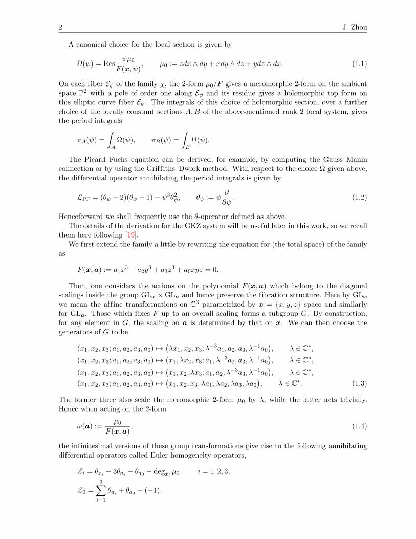
Cx × ρk1Cy, Cx × ρk2Cy have no intersection with the elliptic curve defined by F = 0. Thedifference gives a tubular neighborhood of a certain branch Ck1,k2 of (x, y, z) ∈ F = 0 |x ∈Cx. Then using the residue calculus, one finds a chain integral on the elliptic curve
Iρk1 (ψ)− Iρk2 (ψ) =
∫Cx×(ρk1Cy−ρk2Cy)
ψµ0F
=
∫Cx
Resψµ0F
∣∣∣Ck1,k2
, k = 0, 1, 2. (2.13)
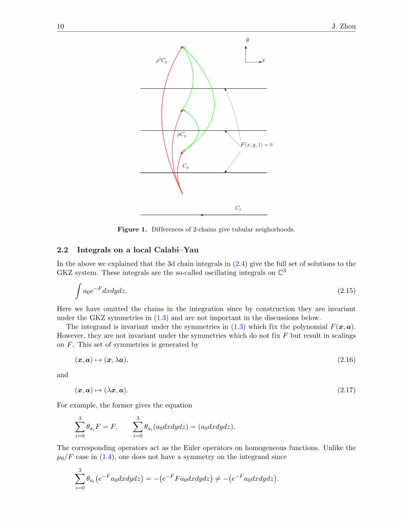
See Fig. 1 for an illustration.It is a classical result, see [2, 14], that the Hesse pencil arise as the equivariant embedding
of elliptic curves with 3-torsion structure to the projective plane via the theta functions. Hereequivariance means that the action of translations by the group E[3] of 3-torsion points (whichare lattice points in 1
3(Z⊕Zτ) if the elliptic curve is realized as E = C/(Z⊕Zτ)) on the curve Egets mapped to projective transformations on P2. Using the particular choices for the thetafunctions in [14], these projective transformations are
σ1 =1
3: (x, y, z) 7→
(x, ρy, ρ2z
),
σ2 =τ
3: (x, y, z) 7→ (y, z, x). (2.14)
The zeros of the coordinate functions x, y, z correspond to those of the theta functionsused to define the embedding. Hence the difference between any two of them (in particularthe endpoints of Ck1,k2) are nothing but the 3-torsion points on the elliptic curve. Using thetranslations in (2.14) which fixes ψ, the chain Ck1,k2 in (2.13) can then produce full cycles.This shows that the difference of the chain integrals given in (2.13) essentially give the periodintegrals.
10 J. Zhou
Cy
ρCy
ρ2Cy
Cx
x
y
F (x, y, 1) = 0
Figure 1. Differences of 2-chains give tubular neighorhoods.
2.2 Integrals on a local Calabi–Yau
In the above we explained that the 3d chain integrals in (2.4) give the full set of solutions to theGKZ system. These integrals are the so-called oscillating integrals on C3∫
a0e−Fdxdydz. (2.15)
Here we have omitted the chains in the integration since by construction they are invariantunder the GKZ symmetries in (1.3) and are not important in the discussions below.
The integrand is invariant under the symmetries in (1.3) which fix the polynomial F (x,a).However, they are not invariant under the symmetries which do not fix F but result in scalingson F . This set of symmetries is generated by
(x,a) 7→ (x, λa), (2.16)
and
(x,a) 7→ (λx,a). (2.17)
For example, the former gives the equation
3∑i=0
θaiF = F,3∑i=0
θai(a0dxdydz) = (a0dxdydz).
The corresponding operators act as the Euler operators on homogeneous functions. Unlike theµ0/F case in (1.4), one does not have a symmetry on the integrand since
3∑i=0
θai(e−Fa0dxdydz
)= −
(e−FFa0dxdydz
)6= −
(e−Fa0dxdydz
).
GKZ Hypergeometric Series for the Hesse Pencil 11
That is, the transformations in (2.16), (2.17), which are redundant for µ0/F when the Calabi–Yau condition (1.10) holds, do not seem to yield symmetries for e−Fdxdydz. However, one knowsfrom the explicit computations that the chain integrals in (2.15) do generate the full space ofsolutions to the GKZ system and hence should be invariant under these transformations.
To resolve this conflict, we are led to the following more correct interpretation of the oscil-lating integral in (2.15). First we note that the above two transformations (2.16), (2.17) arerelated by a transformation which does preserve F , hence we only need to consider one of them.For simplicity, we focus on the latter. Motivated by [43], we think of the above integral as oneon the total space of KP2 . We choose s(a) to be coordinate on the fiber with respect to thetrivialization a0µ0. Note that a0µ0 fails to represent a nonzero section precisely at the orbifoldpoint a0 = 0 on the base of the elliptic curve family. This is why the coordinate s(a) is modulidependent in order to render s(a)a0µ0 well-defined. Then the holomorphic top form on KP2 isa0µ0 ∧ ds(a). Now we consider the differential form on the CY threefold KP2
e−sF (x,a)a0µ0 ∧ ds(a).
Since s(a)a0µ0 gives a meromorphic section of KP2 → P2, under the C∗-actions in (2.16), (2.17)the quantity s(a)F is invariant.
We regard W = sF as a function in the coordinate ring of the variety KP2 . It follows thatthe Calabi–Yau condition (1.10) simply means that W is homogeneous of degree one in the fibercoordinate s
ν := degs(W ) = 1.
This way of looking at the scaling behavior of the form µ0 is convenient, especially when thereis no term a0
∏xi involved in the polynomial F which was used to absorb the shift in (1.5) that
comes from the action on the µ0 part.One can then compute the resulting integral as follows∫ ∞
0
∫e−sFa0µ0 ∧ ds =
∫1
Fa0µ0. (2.18)
In particular, in the patch z = 1, one has∫ ∞0
∫e−(sz
3) Fz3 a0d
(xz
)∧ d(yz
)∧ ds.
Now one can formally make the change of variable sz3 7→ z3, as a computational shortcut, thenthe above integral becomes∫ ∞
0
∫e−F 3a0 dx ∧ dy ∧ dz.
This gives the oscillating integrals discussed earlier in (2.15).In sum, in order to respect all of the GKZ symmetries, the integral in (2.15) should be
interpreted as one on KP2 . In doing actual computations, we shall however think of the integralas if it is on C3 for convenience.
For the 3d chain integral in (2.4), according to (2.18), one gets the 2d real integral which inthe affine coordinate z = 1 becomes∫ ∞
0
∫ ∞0
a0dxdy
F (x, y, 1;ψ). (2.19)
The resulting 2d chain is interpreted in [26] as an element in the relative homology H2(P2 −E,∆−E ∩∆), where ∆ = xyz = 0. Similar examples are discussed in [7] in which the pencil ofcubic curves have base points lying on the integral domain and a blow-up is needed.
12 J. Zhou
3 Chains on the elliptic curves and orbifold singularities
It will be more satisfactory if one can find chains in the elliptic curve fibers that give rise tothe extra solutions to the GKZ system. As mentioned above, this will then establish a linkbetween the oscillating integrals (2.15) in the singularity theory and objects in the elliptic curvegeometry. Since the integral contour in (2.19) is not a tubular neighborhood of a chain on theelliptic curve, a direct dimension reduction is not available.
Instead, we shall first derive an integral formula for the extra solution basing on the in-homogeneous Picard–Fuchs equation and the Wronskian method. The relation to modularforms, which is special in the current example, gives an Eichler integral. Also the integralformula offers a nice interpretation of the extra solution in terms of the Beltrami differentialwhich captures the deformation of complex structures.
Independently, we obtain a chain integral on the elliptic curve for the extra solution, motivatedby the special role played by the orbifold singularity in the moduli space.
3.1 Wronskian method: Eichler integral
We use the Wronskian method to obtain an Eichler integral formula for the solution I(ψ) fol-lowing [7, 15, 16]. Recall that the extra solution I(ψ) to DGKZ in (1.8) must solve the in-homogeneous Picard–Fuchs equation(
θ2ψ − ψ−3(θψ − 2)(θψ − 1))
= C
for some constant C. Taking any basis of the periods u1, u2 annihilated by the Picard–Fuchsoperator LPF in (1.2), then according to the standard Wronskian method one has
Theorem 3.1. The solutions I(ψ) to the GKZ system for the Hesse pencil are given by
I(ψ) = au1(ψ) + bu2(ψ) + c
∫ ψ 1
(1− v−3)v21
W (v)(u1(ψ)u2(v)− u2(ψ)u1(v))dv, (3.1)
for some constants a, b, c.
The lower bound in the integral does not matter: two different choices for the lower boundresult in a change on a, b.
The Wronskian
W (ψ) = (u′1(ψ)u2(ψ)− u1(ψ)u′2(ψ))
can be easily computed by using the Schwarzian of the Picard–Fuchs equation.
It is known that the Hesse pencil is parametrized by the modular curve Γ0(3)\H∗ whoseHauptmodul α(τ) can be found, e.g., in [36]. We take the basis u1, u2 to be the periodsω0(α), ω1(α) near the infinity cusp given in (2.12), with [5] τ = ω1/ω0. See [40] for a collectionof the formulas. Now the last term in (3.1) is∫ α 1
v2(1− v)
1
W (v)(ω0(v)ω1(α)− ω0(α)ω1(v))dv
= ω0(α)
∫ α 1
v2(1− v)
1
W (v)ω0(v)(τ(α)− τ(v))dv,
up to a constant multiple. Then we get
GKZ Hypergeometric Series for the Hesse Pencil 13
Corollary 3.2. Denote the normalized period I/ω0 by tGKZ, then one has the following Eichlerintegral expression of tGKZ near the infinity cusp
tGKZ = a+ bτ + c
∫ α 1
v2(1− v)
1
W (v)ω0(v)(τ(α)− τ(v))dv
= a+ bτ + c
∫ τ
(1− α(v))ω30(v)(τ − v)dv, (3.2)
for some constants a, b, c.
The above formula in (3.2) is consistent with the result that
LGKZ(ω0tGKZ) = θα LPF(ω0tGKZ) = θα 1
(1− α)ω30
∂2τ tGKZ = 0.
Different choices for the reference point in the Eicher integral will affect the last term bya quantity whose second derivative in τ vanishes and hence is a period integral.
We now relate the solutions to modular forms. From (3.2) it follows that
∂2τ tGKZ = c(1− α)ω30, (3.3)
for some constant c. Moreover, the quantity (1 − α)ω30 is equal to the following modular form
of weight 3 for the modular group Γ0(3)
B(τ) =η(τ)3
η(3τ),
see [36] for details. See also [44] for detailed discussions on the computations on periods. In (3.3),when c = 0 one gets the period integrals, otherwise one gets the extra solution to the GKZsystem. For simplicity, we set c = 1 below. The modular form B3 has a nice Eisenstein seriesand hence Lambert series formula given by
B3(τ) = 1− 9∑n≥1
χ−3(n)n2qn
1− qn , q = exp(2πiτ).
Here χ−3 is the Legendre symbol which takes the values 0, 1, −1 on integers of the form 3k,3k + 1, 3k + 2, respectively. Hence we obtain
tGKZ =1
2τ2 + bτ + a+ 9
∑n≥1
χ−3(n)Li2(qn). (3.4)
Remark 3.3. The normalized period tGKZ should be contrasted to the flat coordinate t forthe mirror of the A-model geometry of KP2 , which is a normalized period solved from the 3rdorder Picard–Fuchs equation in (1.12) and arises as the integral of the Mahler measure [41]. Itsatisfies θαt = ω0. By using the Schwarzian this becomes
∂τ t = cB(τ)3, (3.5)
for some constant c. By using its expected boundary behavior, one gets
et = −q∏n≥1
(1− qn)9nχ−3(n), q = e2πiτ .
The inversion of this quantity carries interesting enumerative meaning in Gromov–Witten theory.See [38, 41, 45] for detailed discussions.
14 J. Zhou
By comparing (3.3) with (3.5), and using the properties of the special geometry [42] on themoduli space, one can see that tGKZ is actually related to the quantum volumes of cycles [24]in the A-model Calabi–Yau geometry under mirror symmetry. To be a little more detailed,denoting the prepotential by F (t), then the quantum volumes are given by the normalizedperiods 1, t, ∂tF (t), 2F (t)− t∂tF (t). The normalized solutions to the GKZ system are then, upto unimportant terms,
1 = ∂t(t), τ = ∂t(∂tF (t)),
tGKZ(τ) = −∂t (2F (t)− t∂tF (t)) = t∂t(∂tF (t))− ∂tF (t).
An amusing observation is that tGKZ(τ) is the Legendre dual of ∂tF (t) and vice versa.Since in the current example the Yukawa coupling, which is defined to be ∂3t F (t) = ∂tτ ,
is non-vanishing, we can write a derivatives in τ in terms of that in t. Ignoring the overallmultiplicative factors, and focusing on the normalized periods, we get the simplifications
DGKZ = ∂τ ∂τ
∂t ∂2τ = ∂τ∂t∂τ ∼ ∂t ∂t∂τ , (3.6)
LCY3 = ∂t ∂t
∂τ ∂t ∂t = ∂t∂τ ∂t. (3.7)
We shall say more about the relation between them in Section 4.
Remark 3.4. Since the oscillating integral ω0tGKZ appears naturally in the Landau–GinzburgB-model, in particular, through the Frobenius manifold structure, it is natural to ask whether thenormalized period tGKZ is also related to the enumerative geometry of the mirror LG A-model,similar to the flat coordinate t for the mirror of the A-model geometry of KP2 .
The solution displayed in (3.4) agrees with the fact that the solutions of the GKZ systemmust contain a solution with log2 α behavior. The latter reflects that the indicial equationhas three roots 0, 0, 0 at the point α = 0 (around which a basis of solutions can be obtainedvia Frobenius method). The indeterminacy a, b indicates that the extra solution is subject toaddition by the other two solution which are periods and do not affect the log2 α behavior.For a given solution, say J3, the constants a, b, c in (3.2) can be fixed following the standardmethod. We shall not do this here. Instead, we discuss the representation of the extra solutionnear the orbifold point ψ = 0 around which qualitatively analyzing the solutions is convenientsince the local monodromy action can be diagonalized.
We compute the Wronskian and get,
W (ψ) = ψ2(1− ψ3
)−1.
We take the basis of solutions u1, u2 to be the ones π1, π2 in (2.11). Then we obtain
I(ψ) = aπ1(ψ) + bπ2(ψ) + c
∫ ψ
v−1(π1(ψ)π2(v)− π2(ψ)π1(v))dv,
The local uniformizing variable near the orbifold point ψ = 0 on the base B can be taken to bes = π2/π1. Then in terms of s one has
Corollary 3.5. The local expansion of the solutions to the GKZ system for the Hesse pencilnear the orbifold point is given by
I(s) = aπ1(s) + bπ2(s) + c
∫ s
v−1(π1(s)vπ2(v)− sπ1(s)π1(v))dψ
ds(v)dv
= aπ1(s) + bsπ1(s) + cπ1(s)
∫ s
v−1π1(v)(v − s)dψds
(v)dv.
GKZ Hypergeometric Series for the Hesse Pencil 15
Now it suffices to discuss the integral J3 in terms of the above form since the other twosolutions are period integrals which are solutions to the homogeneous Picard–Fuchs equation.Hence we want to determine the constants a, b, c in the equality
ψ33F2
(1, 1, 1;
4
3,5
3;ψ3
)= aψ 2F1
(1
3,1
3;2
3;ψ3
)+ bψ2
2F1
(1
3,1
3;2
3;ψ3
)+ c
∫ ψ
0v−1
(ψv2 2F1
(1
3,1
3;2
3;ψ3
)2F1
(2
3,2
3;4
3; v3)
− ψ2v 2F1
(1
3,1
3;2
3; v3)
2F1
(2
3,2
3;4
3;ψ3
))dv.
We then use the series formula for hypergeometric functions. Without doing any calculations,we can see that due to the monodromy behavior near ψ = 0, we must have a = b = 0. Then bycomparing the coefficients of ψ3, we are led to
c = −2.
Therefore, the in-homogeneous contribution in the solution in terms of the Wronskian gives themonodromy invariant chain integral J3.
Again this approach singles out the special role of the orbifold point where the gauged sym-metry in (2.8) results in the monodromy (under which the solutions have different behaviors).
3.2 Wronskian method: vanishing periods and Beltrami differential
We now give a geometric interpretation of the last term in (3.1) obtained by the Wronskianmethod
J(α) :=
∫ α 1
v(u1(v)u2(α)− u1(α)u2(v))dv.
This naturally lives in the homology of the total space of the elliptic curve fibration, similar tothe integral over the Lefschetz thimble.
To see this, we choose γ1, γ2 to be any locally constant basis of H1(E,Z) which can bethought of as coming from the marking m : H1(E,Z) ∼= Z2 for a generic reference fiber. Weagain take Ω(v) to be the section of the Hodge line bundle specified in (1.1). The period integralsover the two cycles γ1, γ2, with respect to Ω(v), gives a basis u1(v), u2(v) of solutions to thePicard–Fuchs equation. Then we rewrite J(α) as
J(α) =
∫ α 1
vdv
∫γ(v;α)
Ω(v), γ(v;α) = u2(α)γ1 − u1(α)γ2.
Fixing α, the cycle γ(v;α) is locally constant in v due to parallel transport. It is singled out,up to a constant multiple, by the condition∫
γ(α;α)Ω(α) = 0. (3.8)
That is, away from the orbifold point in the moduli space, it is exactly the unique cyclein H1(Eα,C) which is the Poincare dual of Ω(α) and hence gives the vanishing period in thefiber Eα.
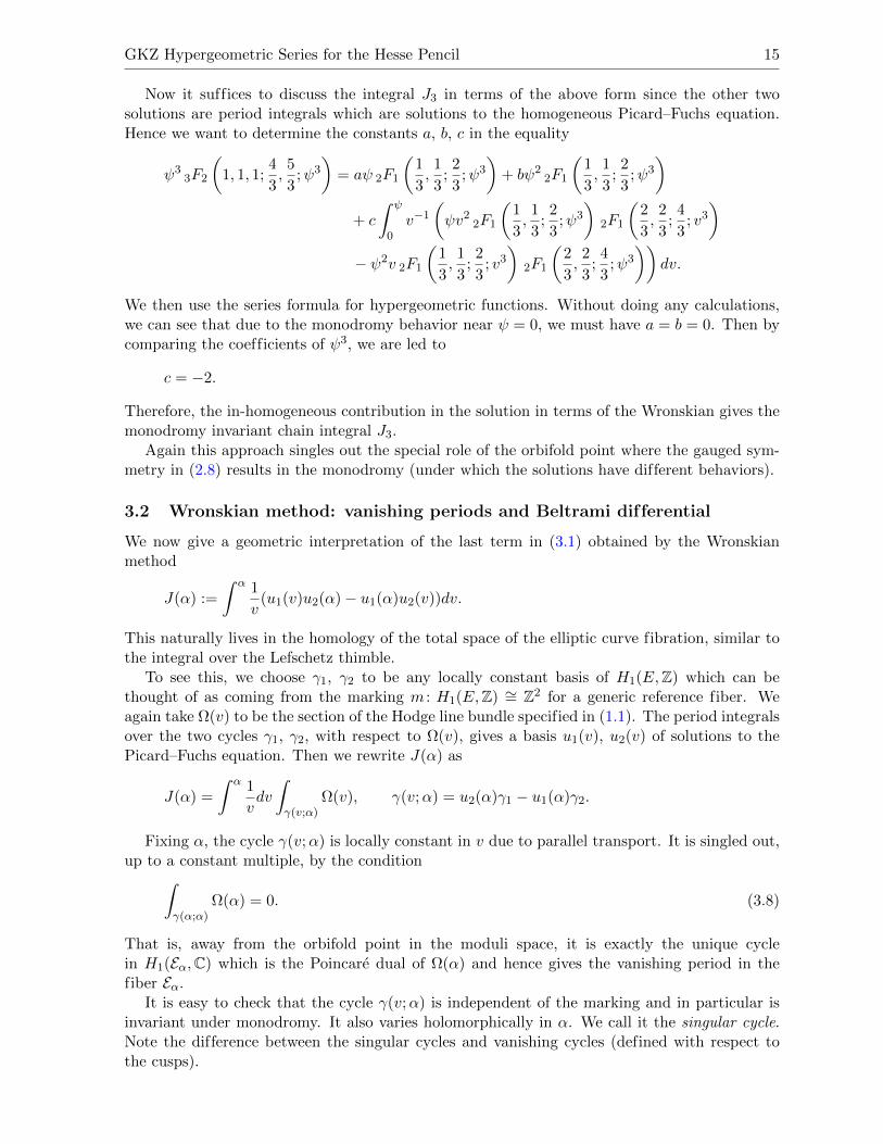
It is easy to check that the cycle γ(v;α) is independent of the marking and in particular isinvariant under monodromy. It also varies holomorphically in α. We call it the singular cycle.Note the difference between the singular cycles and vanishing cycles (defined with respect tothe cusps).
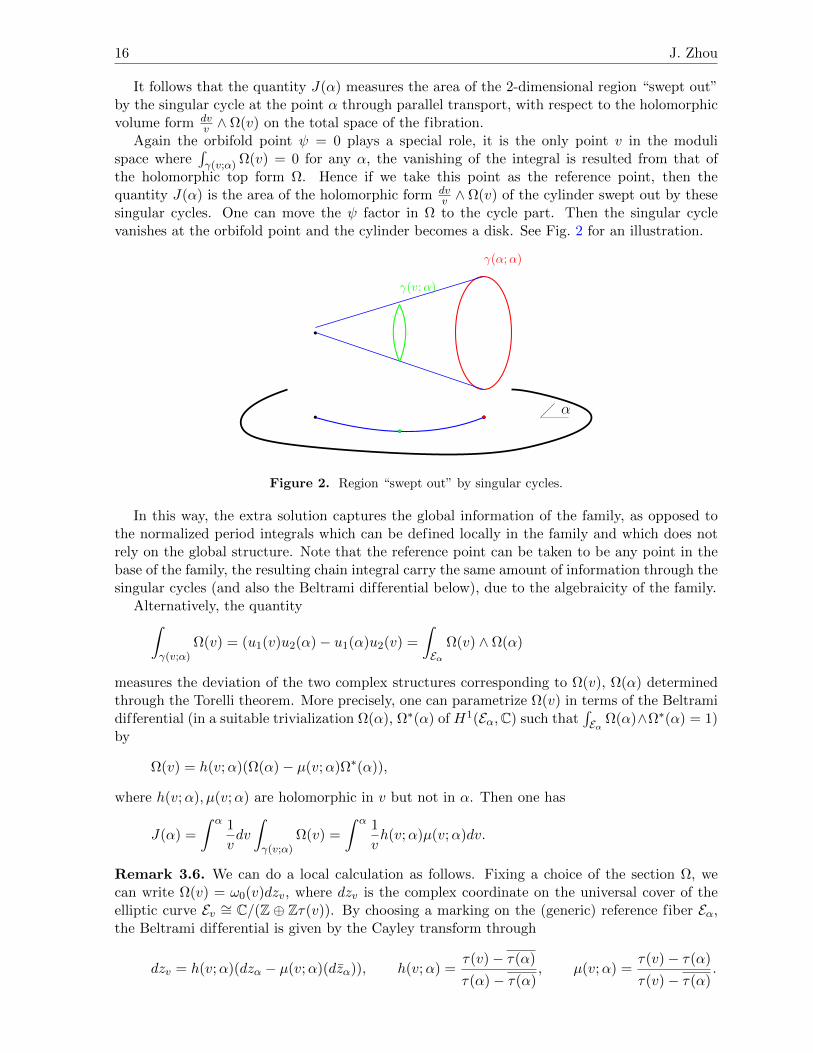
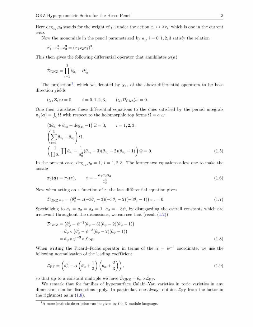
16 J. Zhou
It follows that the quantity J(α) measures the area of the 2-dimensional region “swept out”by the singular cycle at the point α through parallel transport, with respect to the holomorphicvolume form dv
v ∧ Ω(v) on the total space of the fibration.Again the orbifold point ψ = 0 plays a special role, it is the only point v in the moduli
space where∫γ(v;α) Ω(v) = 0 for any α, the vanishing of the integral is resulted from that of
the holomorphic top form Ω. Hence if we take this point as the reference point, then thequantity J(α) is the area of the holomorphic form dv
v ∧ Ω(v) of the cylinder swept out by thesesingular cycles. One can move the ψ factor in Ω to the cycle part. Then the singular cyclevanishes at the orbifold point and the cylinder becomes a disk. See Fig. 2 for an illustration.
α
γ(v;α)
γ(α;α)
Figure 2. Region “swept out” by singular cycles.
In this way, the extra solution captures the global information of the family, as opposed tothe normalized period integrals which can be defined locally in the family and which does notrely on the global structure. Note that the reference point can be taken to be any point in thebase of the family, the resulting chain integral carry the same amount of information through thesingular cycles (and also the Beltrami differential below), due to the algebraicity of the family.
Alternatively, the quantity∫γ(v;α)
Ω(v) = (u1(v)u2(α)− u1(α)u2(v) =
∫Eα
Ω(v) ∧ Ω(α)
measures the deviation of the two complex structures corresponding to Ω(v), Ω(α) determinedthrough the Torelli theorem. More precisely, one can parametrize Ω(v) in terms of the Beltramidifferential (in a suitable trivialization Ω(α), Ω∗(α) of H1(Eα,C) such that
∫Eα Ω(α)∧Ω∗(α) = 1)
by
Ω(v) = h(v;α)(Ω(α)− µ(v;α)Ω∗(α)),
where h(v;α), µ(v;α) are holomorphic in v but not in α. Then one has
J(α) =
∫ α 1
vdv
∫γ(v;α)
Ω(v) =
∫ α 1
vh(v;α)µ(v;α)dv.
Remark 3.6. We can do a local calculation as follows. Fixing a choice of the section Ω, wecan write Ω(v) = ω0(v)dzv, where dzv is the complex coordinate on the universal cover of theelliptic curve Ev ∼= C/(Z ⊕ Zτ(v)). By choosing a marking on the (generic) reference fiber Eα,the Beltrami differential is given by the Cayley transform through
dzv = h(v;α)(dzα − µ(v;α)(dzα)), h(v;α) =τ(v)− τ(α)
τ(α)− τ(α), µ(v;α) =
τ(v)− τ(α)
τ(v)− τ(α).
GKZ Hypergeometric Series for the Hesse Pencil 17
It follows that, as already computed from the Wronskian method,∫γ(v;α)
Ω(v) = −(τ(v)− τ(α))ω0(v)ω0(α).
As pointed out above, the orbifold singularity point has the special property that there aretwo linearly independent vanishing periods corresponding to π1(α), π2(α) in (2.11), while fora generic point α one has only one cycle such that (3.8) is satisfied.
The limit of the singular cycles at the orbifold point can be computed directly throughthe period calculation as follows. Since the singular cycle is independent of the marking, forcomputations we take A, B to be the monodromy invariant cycles at the infinity cusp and zerocusp respectively. There is no ambiguity in A, B at the two cusps respectively, but they of coursesuffer non-trivial monodromies elsewhere. Their period integrals are as displayed in (2.12)
ω0(α) = π1(α) + π2(α), ω1(α) = −ρκπ1(α) + ρ2κπ2(α).
It follows that near the orbifold point α =∞ or equivalently ψ = 0 (here κ = i/√
3)
γ(α;α) = A
∫B
Ω(α)−B∫A
Ω(α) = π1(α)(−ρκA−B) + π2(α)(ρ2κA−B
).
It is this particular linear combination of cycles that the nearby singular cycles converge to atthe orbifold singularity.
3.3 Chains on the elliptic curves and orbifold singularitieson the moduli space
In this section, we shall find a chain C(ψ) on the elliptic curve Eψ so that the resulting integral∫C(ψ) Ω(ψ) gives the extra solution to the GKZ system other than the period integrals.
3.3.1 Weierstrass model
We first motivate the discussion by reviewing the well-studied example of Weierstrass family ofelliptic curves.
As mentioned above in Section 1, the derivation of differential operators from GKZ symme-tries can be applied to any family of algebraic varieties. In particular, we can apply the samediscussion to the Weierstrass family
Y 2 = 4X3 − g2X − g3.
The GKZ operator is computed to be
θw
(θw −
1
4
)(θw −
1
2
)− w
(θw +
3
4
)(θw +
1
12
)(θw +
5
12
),
w = 1− 1728
j= 27
g23g32.
The discussion by [15, 16] implies that the extra solution is provided by the following chainintegral∫ ∞
0
dX
Y=
∫ [P(0),P ′(0),1]
[P(z0),P ′(z0),1]
dX
Y, (3.9)
18 J. Zhou
where z0 is such that ±z0 are zeros of the Weierstrass P-function. When pulled back to thecomplex z-plane (as the universal cover of the elliptic curve) via the Weierstrass embedding, theextra solution above is half of the chain integral∫ z0
−z0dz, (3.10)
where dz is the standard holomorphic top form on the complex z-plane.This singles out the special role of the point determined by g3 = 0 corresponding to the
orbifold point w = 0 in the moduli space, at which the chain z0− (−z0) on the complex z-planevanishes. Intuitively, what is happening is that if one thinks of the elliptic curve as a 2 : 1cover over the x-plane, the chain integral mentioned above measures the “distance” of the twocovering sheets. Its vanishing does not create a change in the topology as it does not lead toa singular curve. However, since the value of g3 is non-vanishing nearby but is vanishing at theorbifold point, the vanishing of the chain integral does reflect a change in the complex structure.
Remark 3.7. This chain integral is actually the Abel–Jacobi map attached to the divisor q− pgiven by the above two points. It appears in the study of the mixed Hodge structure of thesingular curve
Y 2 =(4X2 − g2X − g3
)X2,
and is the obstruction to the isomorphism between the mixed Hodge structure of this singularcurve and the Hodge structure of its normalization, i.e., the Weierstrass curve. Furthermore, itis the limit of a period for the genus two curve obtained by deforming the above singular curve.See [11] for a nice account of discussions on this.
A more natural way to look at the extra solution is to expand the corresponding oscillatingintegral around the orbifold point w = ∞ or equivalently g2 = 0. The reason is that whenperforming the oscillating integral one is led to the following procedure (by applying change ofvariables)∫
e−Y2Z+4X3−g2XZ2−g3Z3
dXdY dZ
=⇒∫Z−
12 e−Y
2e4X
3e−g2XZ
2e−g3Z
3dXdY dZ
=⇒∫Z−
12 g− 1
33 e−Y
2e4X
3e−Z
3∞∑k=0
(−g2g
− 23
3 XZ2)k
k!dXdY dZ.
Here the integral contour needs to be chosen appropriately to deal with the convergence issue.As one can see, evaluating the integral not only provides series solutions to the GKZ system, butalso picks out the natural coordinate for the expansion. From the discussion about the gaugedsymmetries in (2.8), it is easy to see that the orbifold point is always singled out according towhere the polynomial F becomes a Fermat type under a suitable coordinate change. Also thedegree of the DGKZ-operator can be read off easily from the action of the gauged symmetrieswhich in particular induces action on the integral contours. This is in agreement with the resultobtained by examining the linear relations in the toric data for hypersurfaces in toric varietiesfor example.
Therefore, both to see the gauged symmetries and to match the expansion parameter, wethink of the Weierstrass elliptic curve as a 3 : 1 cover over the Y -plane. For a generic member,there are four simply-branched points determined by, setting f(X,Y ) = Y 2− (4X3− g2X− g3),
f = 0, fX = 0,
GKZ Hypergeometric Series for the Hesse Pencil 19
as well as one 2-branched point at Y =∞. The Deck group action (or the Galois action) on thecovering sheets gets enhanced exactly when the simply-branched points collide. That is, whenthe system
f = 0, fX = 0, fXX = 0.
has non-trivial solutions. This is possible exactly at the orbifold point where g2 = 0. The foursimply-branched points now become two 2-branched points Yo determined by
Y 2o = −g3.
Now we can reinterpret the chain integral in (3.9) or (3.10) as the following one, which isnaturally defined on the 3 : 1 covering,
−∫ Yo
−Yo
dY
fX,
where the integral contour above means any sheet covering a path connecting the two points−Yo, Yo which may or may not pass through the branch points.
Note that carrying out the same consideration to the 2 : 1 cover over the X-plane can onlysee the cusp singularities other than the orbifold singularity. As a result one can not get the fullaction of the gauged symmetries from the 2 : 1 cover picture.
3.3.2 Hesse pencil
The above discussion suggests that the oscillating integral sees the finest possible informationof the gauged symmetries by exhibiting the most possible solutions with different monodromybehaviors. They are reflected via the Galois symmetries of the covering with the highest possibledegree.
By analogy, for the Hesse pencil, we look at the orbifold singularities in the moduli spacewhere the configuration of branch points changes. A natural candidate for the chain whoseintegral gives rise to the extra solution to the GKZ system would then be the path connectingpoints which are not branch points for generic values of the modulus but become so at theorbifold point.
We regard a generic member of the Hesse pencil as a 3 : 1 cover over the x-plane, in theaffine patch z = 1. There are 6 simply-branched points xb determined by the equation(
x3b + 1)3
= 4ψ3x3b . (3.11)
We denote the 6 solutions by
xb,1, xb,2 = ρx1, xb,3 = ρ2x1, xb,4 =1
x1, xb,5 =
1
x2, xb,6 =
1
x3.
The symmetry of the elliptic curve for a generic value of ψ given in (2.14) is closely relatedto Galois symmetry of (3.11). To be more precise, the action σ1 in (2.14) induces
γ3 : (x, y) 7→ (ρx, ρ2y).
The Z2 action on the complex plane as the universal cover of the elliptic curve induces (x, y) 7→(y, x). Combing this with the σ2 action in (2.14), one gets a symmetry of the covering
γ2 : (x, y) 7→(
1
x,y
x
).
20 J. Zhou
These actions are the Galois symmetries µ3 × µ2 (3.11) defining the branch variety (not theDeck group transform of the 3 : 1 covering).
Above a branch point xb, the covering has three sheets determined through
y3 − 3ψxby +(x3b + 1
)= (y − yb)2(y + 2yb), y2b = ψxb.
The Deck group of the covering is µ2. This group gets enhanced at the point ψ = 0, with yb = 0.It contains the further symmetry
(x, y, z) 7→ (x, ρy, z), (3.12)
which only exists on the fiber corresponding to orbifold singularity ψ = 0 (where the ellipticcurve has the extra symmetry). Note that there are other points ψ3 = 1,∞ such that the branchvariety (3.11) degenerates, but at these points the elliptic curve fibers become singular and the3 : 1 coverings are only rational maps.
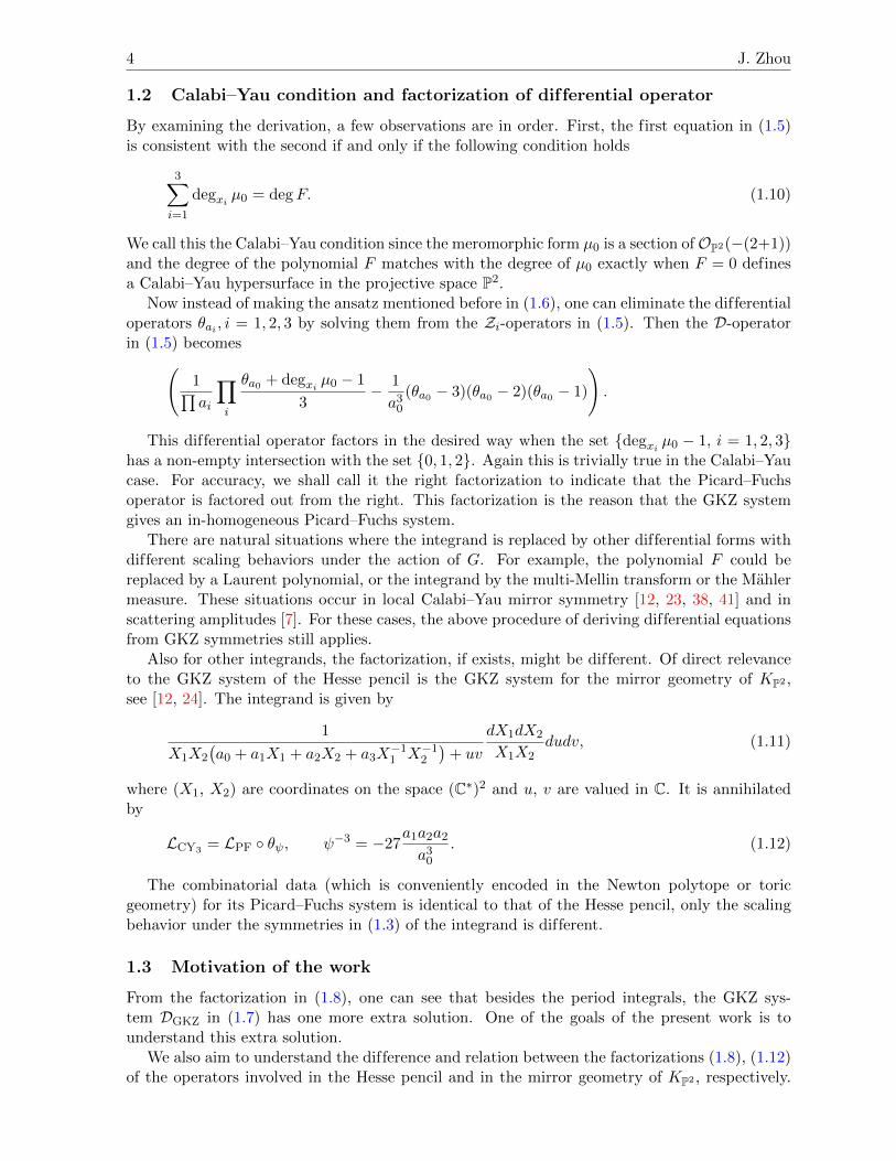
It is easy to see that the branch points given by xb,k, xb,k+3 collide and gives xo,k = −ρk,l = 1, 2, 3 at the orbifold point ψ = 0. Now on a generic fiber, above the point xo,k, thecorresponding y-values of the points on the elliptic curve satisfy
y3o,k − 3ψxo,kyo,k +(x3o + 1
)= y3o,k − 3ψxo,kyo,k = 0.
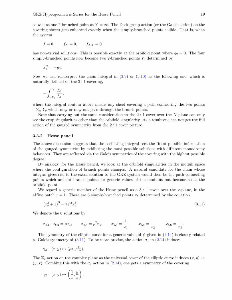
The solution yo,k = 0 gives a 3-torsion point on the elliptic curve. The other two solutions satisfyy2o,k = 3ψxo,k. See Fig. 3 for an illustration of the degeneration of the branch variety.
x
Cx
ρCx
ρ2Cx
xb,1(ψ)
xb,4(ψ)
xb,2(ψ)
xb,3(ψ)
xb,6(ψ)
xb,5(ψ)
C(ψ)
xo,3
xo,2
xo,1
ψ → 0
Figure 3. Branch configuration of the 3 : 1 cover. As ψ → 0, the branch points xb,k, xb,k+3 collide to
xo,k = −ρk, k = 1, 2, 3.
Now for a generic value of ψ, we take a path C(ψ) on the elliptic curve with endpoints
[xo,k, (3ψxo,k)12 , 1], [xo,l, 0, 1], as depicted in Fig. 3. Here k could be the same as l.
GKZ Hypergeometric Series for the Hesse Pencil 21
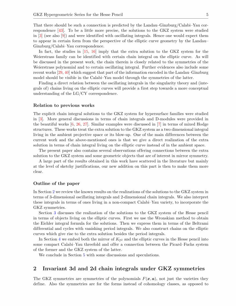
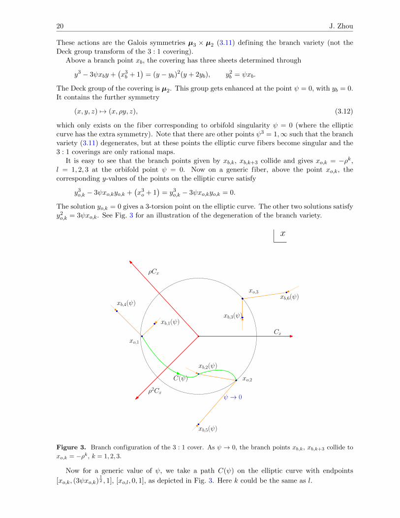
Note that a path like this must pass through a branch point. The difference between twosuch paths are cycles and hence their integrals are differed by period integrals. See Fig. 4 foran illustration.
x
y
C(ψ)
Figure 4. Chain on the elliptic curve passing through a branch point.
Note also that if instead one takes a path with endpoints [xo,k, 0, 1], [xo,l, 0, 1], k 6= l, thenone gets a chain connecting two 3-torsion points and the resulting integral is a period integralas mentioned before in Section 2.1.2.
We consider the chain integral
K(ψ) :=
∫C(ψ)
ψdx
3y2 − 3ψx. (3.13)
We then have the following result.
Theorem 3.8. The integral (3.13) gives a solution to the GKZ system for the Hesse pencil andis not a period integral.
Proof. From the Griffiths–Dwork method, we can find the exact term in the Picard–Fuchsoperator acting on the holomorphic top form to be
(θ2ψ − ψ−3(θψ − 2)(θψ − 1)
)( ψdx
3y2 − 3ψx
)= ψ−3 LPF
(ψdx
3y2 − 3ψx
)= d
(ψx
fy
).
Note that by construction the endpoints of the path C(ψ), when parametrized by x, are locallyconstant and hence annihilated by the derivatives. Then by Stokes theorem, one can immediatelycheck the in-homogeneous Picard–Fuchs equation
(ψ−3 LPF
)K(ψ) =
∫C(ψ)
d
(ψx
y
)=
(ψx
fy
) ∣∣∣∂C(ψ)
=1
6−(−1
9
)6= 0.
Therefore, these chain integrals do give solutions to the GKZ operator DGKZ = θ (ψ−3 LPF)which are not periods.
Remark 3.9. The endpoints of the chain belong to Eψ∩x3+z3 = 0. Under the uniformizationby he θ-functions, see, e.g., [14], these end points are zeros of certain theta functions and
22 J. Zhou
carry interesting arithmetic information, as is the case in the Weierstrass family discussed inSection 3.3.1. In terms of the toric coordinates corresponding to the characters, this is similarto the situation that appears in open mirror symmetry [30, 31, 32, 33, 37] which again seemsto indicate that the chain integral is related to the enumerative geometry in the A-model undermirror symmetry.
Remark 3.10. One can also consider the higher Frobenius functions appearing as the coeffi-cients in the ε-expansion of the function
ω0(α, ε) =∞∑n=0
Q(ε)Γ(3n+ 3ε+ 1)
Γ(n+ ε+ 1)3
( α33
)n+ε:=
∞∑k=0
fk(α)εk, Q(ε) =Γ(ε+ 1)3
Γ(3ε+ 1).
This is the deformation of the period in (2.12) when applying the Frobenius method to solve forthe solutions to the Picard–Fuchs equation. It satisfies, recall (1.9),
LPFω0(α, ε) =( α
33
)εε2, DGKZω0(α, ε) =
( α33
)εε3.
Therefore, one has
LPFfk(α) =(ln α
33)k−2
(k − 2)!, DGKZfk(α) =
(ln α33
)k−3
(k − 3)!.
Here we have used the convention that negative powers of (ln α33
) give zero. Besides f0, f1 whichare period integrals and f0, f1, f2 which are chain integrals, the higher Frobenius functionsfk, k ≥ 3, which can be solved by the Wronskian method as in Section 3.1, are also interestingon their own. For example, they carry interesting arithmetic meanings, corresponding to thecounting of rational points of the Hesse elliptic curves [9, 10]. Furthermore, when one regardsthe variable ε as the hyperplane class of P2, then ω0(α, ε) gives Givental’s (twisted) I-functionvalued in the cohomology ring and the factorQ(ε) is the Γ-class which appears naturally in mirrorsymmetry, see [18, 22, 25, 35]. After passing to the equivariant cohomology corresponding tothe diagonal torus action, the higher Frobenius functions then appear as the coefficients of theequivariant version of the I-function expanded in the equivariant parameter. We wish to discusstheir geometric meanings in a future work.
3.3.3 Legendre family
We conclude this section with some discussions on the Legendre family whose affine equation is
y2 = x(x− 1)(x− λ), j(λ) = 28(λ2 − λ+ 1)3
λ2(λ− 1)2. (3.14)
From the derivation of GKZ system using the GKZ symmetries, we can see that the operatorDGKZ is a 2nd order operator and hence coincides with the Picard–Fuchs operator. This alsoagrees with the earlier discussion on the relation between the extra solution and orbifold sin-gularities. Namely, in this case one can check that the Picard–Fuchs equation has no orbifoldsingularity. One can also see this by using the standard fact that the base of the family isparametrized by the modular curve Γ(2)\H∗ which has no elliptic fixed point.
However, from the evaluation of the oscillating integral, one can see that∫e−(y
2z−(x3−(λ+1)x2z+λxz2))dxdydz
∼ λ− 12
∫e−y
2ex
3ez
2∞∑k=0
(λ+ 1
λ12
)k x 32k− 1
2 zk−12
k!dxdydz.
GKZ Hypergeometric Series for the Hesse Pencil 23
Therefore, the oscillating integral naturally singles out the coordinate α = (λ+ 1)/λ12 for the
expansion parameter.4 Moreover, the gauged symmetries would give rise to at least 6 solutionswith different monodromy behaviors. This is however not a contradiction to the statementthat the DGKZ is of second order. The reason is that in deriving the DGKZ using the GKZsymmetries, only scalings on the parameter λ are allowed and hence those act by scalings onthe new parameter α is not included.
Furthermore, the locus at which α = 0 corresponds to the point λ = −1 or j = 1728 accordingto the formula for the j-invariant in (3.14). Hence indeed when parametrized by α the aboveexpansion of the oscillating integral occurs near an orbifold point.
One can again obtain chain integrals by studying the branch configuration of the 3 : 1 coverrealization for the elliptic curve. Now the enhancement of the Galois symmetry takes place atλ = −ρ,−ρ2 where j = 0. This corresponds to a different way of performing the oscillating theintegral above by first applying the following change of variables and then evaluating
−y2z +(x3 − (λ+ 1)xz2 + λz3
)= −y2z +
(x− λ+ 1
3
)3
+
(λ+ 1
3
)3
z3
−(λ2 − λ+ 1
3
)(x− λ+ 1
3
)z2 − (λ+ 1)(λ2 − λ+ 1)
32z2.
In summary, the oscillating integrals offer more than the solutions to the GKZ systems. It hasthe finest information about the gauged symmetries which includes the GKZ scaling symmetriesas a subset.
4 Period integrals in a compact Calabi–Yau threefold
In this section, we shall explain the relation between the two differential operators, namely DGKZ
in (1.8) and LCY3 in (1.12). We shall see that they are different pieces of the same Picard–Fuchssystem of a compact Calabi–Yau threefold.
Recall that in Section 2.2 we explained that the 3d oscillating integrals and 2d real integralsin (2.18) should be interpreted as ones on a non-compact Calabi–Yau. We now push this ideafurther.
We first note that the members in the Hesse pencil correspond to the sections of the anti-canonical divisor of the toric variety P whose polytope is generated by (1, 0), (0, 1), (−1,−1).This polytope is a reflective polytope and defines the following toric variety
P = P2/G, G =
(ρn1 , ρn2 , ρn3) |n1 + n2 + n3 = 0 mod 3. (4.1)
The invariants of G are the monomials x31, x32, x
33, x1x2x3 among all cubic monomials. The
induced action on a generic member of the Hesse pencil is the one generated by σ1 in (2.14).The quotient therefore gives the 3-isogeny of the Hesse pencil and is the mirror of the Hessepencil according to [4]. It can be checked by using the GKZ symmetries or by evaluating theoscillating integrals that these two elliptic curve families share the same GKZ operators. Hencefor the purpose of studying the solutions to the GKZ system, there is no difference betweenthese two families. See [46] for discussions on these facts and some arithmetic aspects of themirror symmetry.
Now the quotient of the Hesse pencil is naturally interpreted as sections of the canonicalbundle KP of P . There is a natural compactification [8, 12] X of KP . A certain limit of X givesrise to the variety KP , as the mirror of KP2 , whose Picard–Fuchs operator is displayed in (1.12).
4The transformation from the λ-parameter to this α-parameter is induced by a 2-isogeny, as can be seenthrough the elliptic κ-modulus.
24 J. Zhou
This idea is used frequently in the literature to study mirror symmetry for non-compact Calabi–Yau manifolds. As we shall review in Section 4.1, this compactification also encodes the fullinformation of the quotient of the Hesse pencil by G, as the mirror of the Hesse pencil, includingthe GKZ operator DGKZ in (1.8).
It is then natural to expect a relation between the two geometries–mirror of Hesse pencil andmirror of KP2 – by embedding them in the same ambient space X. The properties about theGKZ/Picard–Fuchs system should be independent of the choice for the compactification though.
4.1 Review of the compactification
We now recall the construction of the compactification following [8, 12]. The A-model is anelliptic fibration over P2. The total space X is a Calabi–Yau hypersurface in a toric variety. Forthe mirror geometry X, the toric data gives the family of varieties X whose Zariski open setsare described by the equation
Ξ = b0 + Z23Z
34
(a1Z1 + a2Z2 + a3Z
−11 Z−12 + a0
)+ a4Z
−13 + a5Z
−14 .
Switching to the homogeneous coordinates, this is
Ξ =(∏
x−1i
) (b0x1x2x3x4x5 + a1x
181 + a2x
182 + a3x
183 + a0x
61x
62x
63 + a4x
34 + a5x
25
):=(∏
x−1i
)ξ. (4.2)
It is an elliptic fibration over the base P which is parametrized by x1, x2, x3. We ignore thesubtitles about the group actions involved which do not affect the Picard–Fuchs systems we areinterested in. Thinking of X as a Weierstrass fibration over P , we then get the identificationfor the divisor classes(
x3i = 0), (x1x2x3 = 0) = OWP (1), i = 1, 2, 3,
(x4 = 0) = OWP (2)⊗K−2P , (x5 = 0) = OWP (3)⊗K−3P , (4.3)
where WP denotes the weighted projective space WP[1, 2, 3] in which the elliptic curve fiberssit. This implies that the coefficients transform as sections of certain tensor powers of KP :the variables a4, a5, b0 transform as sections of K−1P , while a1, a2, a3, a0 sections of K−6P .Strictly speaking, they are sections of the corresponding relative line bundles over the base ofthe fibration.
Note that setting a4 = a5 = b0 = 0 in ξ gives the equation for the Hesse pencil. The limitb0 = 0 in ξ gives [12] the mirror of KP2 . We shall say more about this below.
By using the GKZ symmetries, one can simplify ξ into(bx1x2x3x4x5 + x181 + x182 + x183 + ax61x
62x
63 + x34 + x25
).
Here5
a = (a1a2a3)− 1
3a0, b = b0(a1a2a3)− 1
18a− 1
34 a
− 12
5 . (4.4)
There are interesting loci in the base of the family Ξ parametrized by the coordinates (a, b). Inparticular, the point a = b = ∞ corresponds to the large complex structure limit. See [8, 12]and also [1, 28] for details.
5We have used different notations for the parameters from those in [8].
GKZ Hypergeometric Series for the Hesse Pencil 25
4.2 Picard–Fuchs system and fundamental periodof the compactified geometry
The period integrals are the integrals of the following form over the tubular neighborhood ofcycles in X∫
b0Ξ
dZ1dZ2dZ3dZ4
Z1Z2Z3Z4=
∫b0µ0ξ. (4.5)
where µ0 denotes the standard meromorphic 4-form in the ambient space which has a pole oforder one at infinity. The Picard–Fuchs system can be derive from the GKZ symmetries andare given as follows6
D1 =1
(−3)2(−2)3θa0θb0 − ab−6(θb0 − 1)(θb0 − 5),
D2 =1
(−18)3(θb0 + 6θa0)3 − a−3(θa0 − 1)(θa0 − 2)θa0 .
In terms of the coordinates a, b, we get
D1 =1
(−3)2(−2)3θaθb − ab−6(θb − 1)(θb − 5),
D2 =1
(−18)3(θb + 6θa)
3 − a−3(θa − 1)(θa − 2)θa. (4.6)
The fundamental period7 can be obtained directly by manipulating the series expansionin (4.5) with a suitable choice for the integral contour, as done in [8, 12]. It is given by
ω0(a, b) =
∞∑n,m=0
Γ(18n+ 6m+ 1)
Γ(9n+ 3m+ 1)Γ(6n+ 2m+ 1)Γ(n+ 1)3Γ(m+ 1)am(b−6)3n+m
=
∞∑k=0
Γ(6k + 1)
Γ(3k + 1)Γ(2k + 1)Γ(k + 1)b−6kUk(a) :=
∞∑k=0
ckb−6kUk(a), (4.7)
where
Uk(a) = ak[ k3]∑
l=0
Γ(k + 1)
Γ(l + 1)3Γ(k − 3l + 1)a−3l.
The above expansion (4.7) amounts to solving the Picard–Fuchs system (4.6) in the followingway. The degree k-piece ckb
−6kUk(a) in the sum satisfies θb = −6k. Hence the second equationin (4.6) gives the equation for Uk(a)(
1
(−18)3(−6k + 6θa)
3 − a−3(θa − 1)(θa − 2)θa
)Uk(a) = 0.
This can be simplified into((θa − 1)(θa − 2)θa − a3
63
(−18)3(θa − k)3
)Uk(a) = 0.
6These Picard–Fuchs operators are derived by factoring out some differential operators from the left in theGKZ Z-operators. One can also study the extra solutions to the GKZ system of the current Calabi–Yau threefoldby embedding it into a variety of higher dimension, similar to what will be discussed below. But we shall notdiscuss them in this work.
7The unique (up to scaling) regular period near the large complex structure limit given by a = b =∞.
26 J. Zhou
The first equation in (4.6) then gives recursive relations among ckb−6kUk(a)k through∑k
(−6k)b−6kckθaUk =∑k
(−3)2(−2)3ab−6k−6(6k + 1)(6k + 5)ckUk.
This is simplified into
θaUk+1 = (k + 1)aUk.
4.3 Embedding of the GKZ system for the Hesse penciland the Picard–Fuchs system for the mirror geometry of KP2
For the purpose of getting the other solutions via the Frobenius method and doing analyticcontinuation, one needs to extend [8] the definition of Uk to Uν for complex values of ν
Uν(a) = aν∞∑l=0
Γ(ν + 1)
Γ(l + 1)3Γ(ν − 3l + 1)a−3l = aν 3F2
(−ν3,1− ν
3,2− ν
3; 1, 1; a−3
).
It can be analytically continued to the orbifold a = 0 via the Barnes integral formula [8]
Uν(a) =3−1−νρ
ν2
Γ(−ν)
∞∑n=0
Γ(n−ν3 )
Γ2(1− n−ν3 )
(−3ρa)n
n!. (4.8)
The recursive relation is given by
θaUν+1 = (ν + 1)aUν .
It is annihilated by the operator
Lν =
((θa − 1)(θa − 2)θa − a3
63
(−18)3(θa − ν)3
).
Setting a = −3ψ (which makes contact with the Hesse pencil), one gets
Lν =((θψ − 1)(θψ − 2)θψ − ψ3(θψ − ν)3
).
When ν = 0, this is the Picard–Fuchs operator LCY3 in (1.12).When ν = −1, this is equivalent to the operator DGKZ in (1.8) and it annihilates the form µ0
Fin (1.4). The solution given in (4.8) is exactly the one in (2.3) up to a constant multiple.
In general, Lν annihilates
aν+10
µ0F. (4.9)
As explained in Section 2.2, one should think of the parameter a0 (previously denoted by sa0 inthe trivialization µ0) as the coordinate of the fiber of KP , and hence ν + 1 as the degree of theform in (4.9) along the fiber direction.
Consider the analytic continuation of the expansion (4.7) to the orbifold point b = 0, thenone has [8]
ω0(a, b) =1
2π
∞∑k=0
2−12−2k3−
12−3k6
12+6kΓ(k + 1
6)Γ(k + 56)
Γ(k + 1)2b−6kUk(a)
=
∞∑k=0
Γ(k + 16)Γ(k + 5
6)
Γ(k + 1)2(432)kb−6kUk(a) :=
∞∑n=0
dnbnU−n
6(a).
GKZ Hypergeometric Series for the Hesse Pencil 27
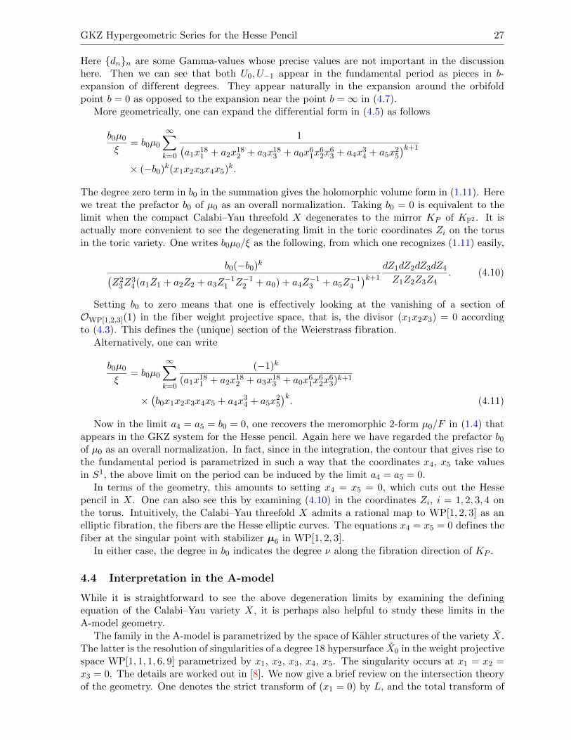
Here dnn are some Gamma-values whose precise values are not important in the discussionhere. Then we can see that both U0, U−1 appear in the fundamental period as pieces in b-expansion of different degrees. They appear naturally in the expansion around the orbifoldpoint b = 0 as opposed to the expansion near the point b =∞ in (4.7).
More geometrically, one can expand the differential form in (4.5) as follows
b0µ0ξ
= b0µ0
∞∑k=0
1(a1x181 + a2x182 + a3x183 + a0x61x
62x
63 + a4x34 + a5x25
)k+1
× (−b0)k(x1x2x3x4x5)k.
The degree zero term in b0 in the summation gives the holomorphic volume form in (1.11). Herewe treat the prefactor b0 of µ0 as an overall normalization. Taking b0 = 0 is equivalent to thelimit when the compact Calabi–Yau threefold X degenerates to the mirror KP of KP2 . It isactually more convenient to see the degenerating limit in the toric coordinates Zi on the torusin the toric variety. One writes b0µ0/ξ as the following, from which one recognizes (1.11) easily,
b0(−b0)k(Z23Z
34 (a1Z1 + a2Z2 + a3Z
−11 Z−12 + a0) + a4Z
−13 + a5Z
−14
)k+1
dZ1dZ2dZ3dZ4
Z1Z2Z3Z4. (4.10)
Setting b0 to zero means that one is effectively looking at the vanishing of a section ofOWP[1,2,3](1) in the fiber weight projective space, that is, the divisor (x1x2x3) = 0 accordingto (4.3). This defines the (unique) section of the Weierstrass fibration.
Alternatively, one can write
b0µ0ξ
= b0µ0
∞∑k=0
(−1)k
(a1x181 + a2x182 + a3x183 + a0x61x62x
63)k+1
×(b0x1x2x3x4x5 + a4x
34 + a5x
25
)k. (4.11)
Now in the limit a4 = a5 = b0 = 0, one recovers the meromorphic 2-form µ0/F in (1.4) thatappears in the GKZ system for the Hesse pencil. Again here we have regarded the prefactor b0of µ0 as an overall normalization. In fact, since in the integration, the contour that gives rise tothe fundamental period is parametrized in such a way that the coordinates x4, x5 take valuesin S1, the above limit on the period can be induced by the limit a4 = a5 = 0.
In terms of the geometry, this amounts to setting x4 = x5 = 0, which cuts out the Hessepencil in X. One can also see this by examining (4.10) in the coordinates Zi, i = 1, 2, 3, 4 onthe torus. Intuitively, the Calabi–Yau threefold X admits a rational map to WP[1, 2, 3] as anelliptic fibration, the fibers are the Hesse elliptic curves. The equations x4 = x5 = 0 defines thefiber at the singular point with stabilizer µ6 in WP[1, 2, 3].
In either case, the degree in b0 indicates the degree ν along the fibration direction of KP .
4.4 Interpretation in the A-model
While it is straightforward to see the above degeneration limits by examining the definingequation of the Calabi–Yau variety X, it is perhaps also helpful to study these limits in theA-model geometry.
The family in the A-model is parametrized by the space of Kahler structures of the variety X.The latter is the resolution of singularities of a degree 18 hypersurface X0 in the weight projectivespace WP[1, 1, 1, 6, 9] parametrized by x1, x2, x3, x4, x5. The singularity occurs at x1 = x2 =x3 = 0. The details are worked out in [8]. We now give a brief review on the intersection theoryof the geometry. One denotes the strict transform of (x1 = 0) by L, and the total transform of
28 J. Zhou
the divisor (x1x2x3 = 0) by H = 3L + E, where E is the class of the exceptional divisor. Theintersections are
H3 = 9, H2L = 3, HL2 = 1, L3 = 0.
Thinking of X as the blow-up, the Kahler classes are linear combinations of L (the strictlytransform of the Kahler class on the singular variety) and the exceptional divisor class E. Thefibration structure also tells that the class of the base P2 is E, the pull back of OP2(1) gives theclass L. One has E ·E · L = −3. This is the degree of the line bundle KP2 over P2. It confirmsthe statement that E is the base P2 of the elliptic curve family. The effective curve classes are
h = L · L, ` = L · E,
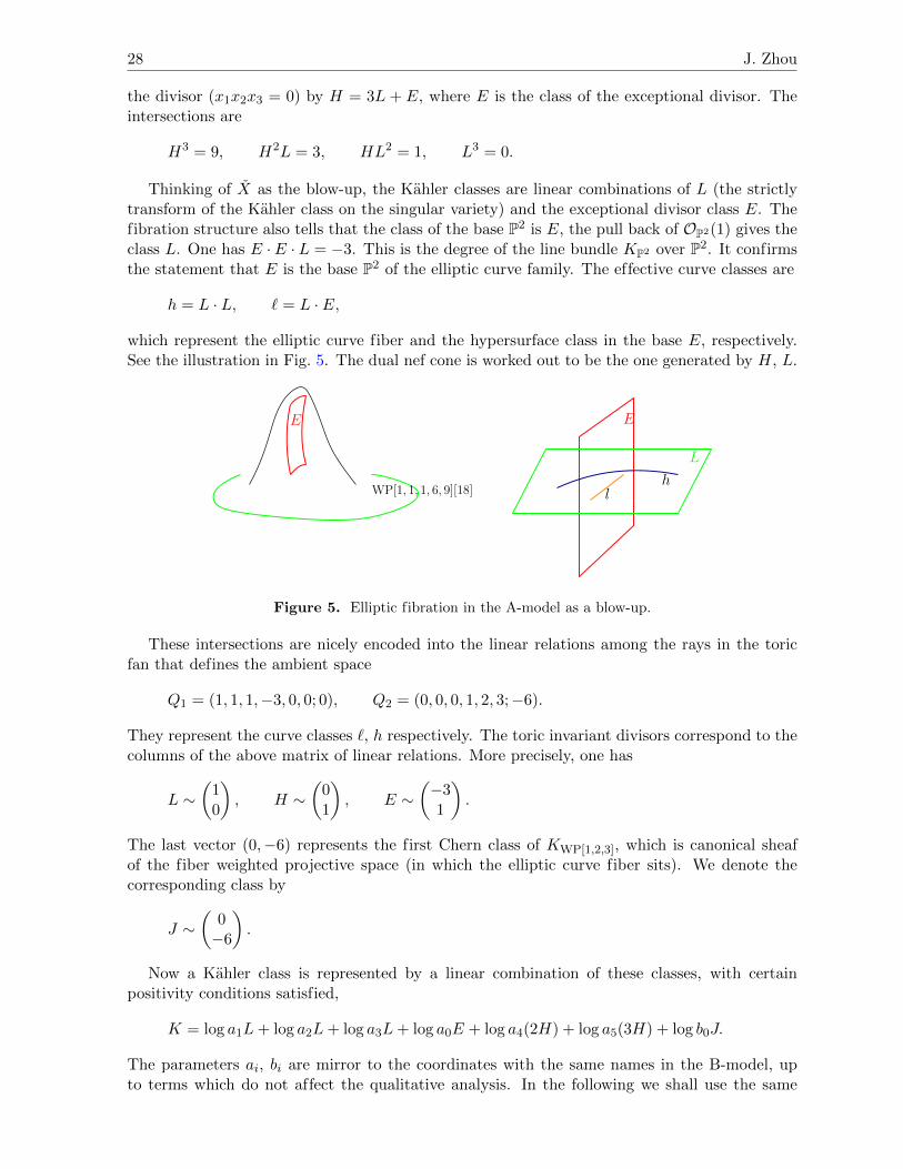
which represent the elliptic curve fiber and the hypersurface class in the base E, respectively.See the illustration in Fig. 5. The dual nef cone is worked out to be the one generated by H, L.
WP[1, 1, 1, 6, 9][18]
E E
L
lh
Figure 5. Elliptic fibration in the A-model as a blow-up.
These intersections are nicely encoded into the linear relations among the rays in the toricfan that defines the ambient space
Q1 = (1, 1, 1,−3, 0, 0; 0), Q2 = (0, 0, 0, 1, 2, 3;−6).
They represent the curve classes `, h respectively. The toric invariant divisors correspond to thecolumns of the above matrix of linear relations. More precisely, one has
L ∼(
10
), H ∼
(01
), E ∼
(−31
).
The last vector (0,−6) represents the first Chern class of KWP[1,2,3], which is canonical sheafof the fiber weighted projective space (in which the elliptic curve fiber sits). We denote thecorresponding class by
J ∼(
0−6
).
Now a Kahler class is represented by a linear combination of these classes, with certainpositivity conditions satisfied,
K = log a1L+ log a2L+ log a3L+ log a0E + log a4(2H) + log a5(3H) + log b0J.
The parameters ai, bi are mirror to the coordinates with the same names in the B-model, upto terms which do not affect the qualitative analysis. In the following we shall use the same
GKZ Hypergeometric Series for the Hesse Pencil 29
coordinates a, b as in (4.4). An element in the nef cone (one of the chambers in the second fanof the toric variety8) must satisfy the condition
K = log
(a1a2a3a30
)L+ log
(a24a
35a0b60
)H
= log(a−3)L+ log
(ab−6
)H ∈ R>0L⊕ R>0H. (4.12)
Therefore the large volume limit corresponds to the point
a−3 = 0 = ab−6, (4.13)
which is mirror to the large complex structure limit mentioned before. Hence one can see thatin the defining equation ξ in (4.2) for the B-model, one needs to send both a, b to ∞.
Now it is easy to see that the limit b0 = 0 corresponds to the degeneration9 of Kahler structureK → L, as when considering for example instanton expansions cycles with infinity volumes aresuppressed. In particular, the class of the elliptic curve fiber h = L · L does not survive thelimit. On the level of toric data or Mori cone of curve classes, the vector Q2 representing theclass h is invisible in the limit and hence what is left is the one Q1 which is exactly the toric datathat defines the geometry KP2 . On the level of geometry, that h has infinite volume tells thatthe elliptic fibration over E gets decompactified to KP2 . This is consistent with the B-modelpicture discussed below (4.10).
Similarly, for the limit a4 = a5 = 0, one has the degeneration K → L. Now the curve class 3`,which is the one underlying the cubic in E ∼= P2 survives this limit. This is also consistent withthe B-model picture discussed below (4.11).
5 Discussions and speculations
For a general Laurent polynomial F , the relations among the monomials are conveniently de-scribed combinatorially by the Newton polytope. This in particular gives a shortcut in derivingthe differential equations.
As mentioned in Section 2.1.2, the difference between the universal family of cubics andthe Hesse pencil is that the latter carries an extra level structure. This is what picks outthe 4 monomials appearing in the Hesse pencil among the all the 10 cubic monomials. These 4monomials is what determines the symmetries of the family and hence the GKZ symmetries.The linear space spanned by them encode the full data of the family.
Instead of using the Veronese embedding of P2 into PH0(P2,O(3)), we use only the 4 mono-mials xyz, x3, y3, z3, i = 1, 2, 3. Consider the partial Veronese map
Φ: P2 → P3, (x, y, z) 7→ (X0, X1, X2, X3) =(xyz, x3, y3, z3
).
The image of P2 is given by the vanishing of the ideal generated by
Φ = X1X2X3 −X30 ,
which defines a singular cubic surface S0 of degree 3 in P3. Here we used the same notation Φto denote the polynomial by abuse of notation. The singular points on S0 are given by
(X0, X1, X2, X3) = (0, 1, 0, 0), (0, 0, 1, 0), (0, 0, 0, 1).
8See, e.g., [13] for a detailed review.9However, in this limit log(ab−6) has a negative sign from the previous limit in (4.13) and the description
in (4.12) for the Kahler class fails. This means that this limit does not sit inside the nef cone of X and it hasmoved deeply into some other chamber in the secondary fan. This situation is typical in the so-called phasetransition process, see [43].
30 J. Zhou
Locally a neighborhood of each singular point is of the form of an A2-singularity describedby C2/Z3. This surface is nothing but the mirror of P2 given by P2/G as described in (4.1). Theelliptic curve is then mapped to the intersection of this cubic surface S0 with the hyperplane
H :=∑
aiXi = 0.
One can alternatively make a moduli dependent embedding by using the monomials aiXi,i = 0, 1, 2, 3, then the moduli dependence of the intersection is full encoded in the moduli de-pendence of the singular cubic surface S0.
The above procedure linearizes the monomials in the defining equation F for the Hesse pencil.The integrand in (2.15) then becomes (up to the a0 factor)
e−Fdxdydz =1
33e−
3∑i=0
aiXiδS0
∏ dXi
X2/3i
:= e−HδS0µ,
where δ means the Dirac delta distribution. As before, the integrand e−sFµ0 ∧ ds on needs tobe suitably interpreted in order to incorporate all the Z-symmetries.
Now the original Z-symmetries become diagonal symmetries of the quadratic form H =∑aiXi. These symmetries also leave the variety S0 invariant (the polynomial Φ is not invariant).
The original D-symmetries are manifest through the Veronese map Φ. Schematically one has
Z(H) = 0, Z(S0) = 0, Z(e−HδS0µ
)= 0, D
(e−HδS0µ
)= e−HδS0Φµ = 0. (5.1)
Note that the characteristic variety (singular support) of D is now defined byp1p2p3 − p30 = 0
⊆ T ∗C4,
where pi, i = 0, 1, 2, 3 are the fiber coordinates of the cotangent bundle of C4 parametrized bya0, a1, a2, a3. This takes the same form as the polynomial Φ. In fact, by restricting the field Cto the field R which does not affect the discussion on GKZ symmetries, one can regard
F(•) =
∫e−H(•)µ
as a formal Fourier transform. Then one has
D = F(Φ).
Note that D has constant coefficients, this then relates Φ to the characteristic variety.
We can also formally write the original oscillating integral over the invariant chain D3 =(0,∞)× (0,∞)× (0,∞) in (2.1) (which produces all solutions under the monodromy action) as
I =
∫D3
e−Fµ0 =
∫D3×(0,∞)
e−HδS0µ = F(δS0).
The configuration (Φ, H) fully encodes the information of the Hesse pencil. Since by a modulidependent embedding one can make H independent of a1, a2, a3, a0, it is therefore very naturalto expect that the GKZ system can be approached via studying the mixed Hodge structure ofS0 together with the moduli-independent hyperplane. The presentation of the GKZ symmetriesin the form displayed in (5.1) also begs for an explanation in terms of D-module in addressingthis problem. A good understanding of this matter is potentially useful in the studies of openmirror symmetry where similar situation occurs, see, e.g., [34, 37].
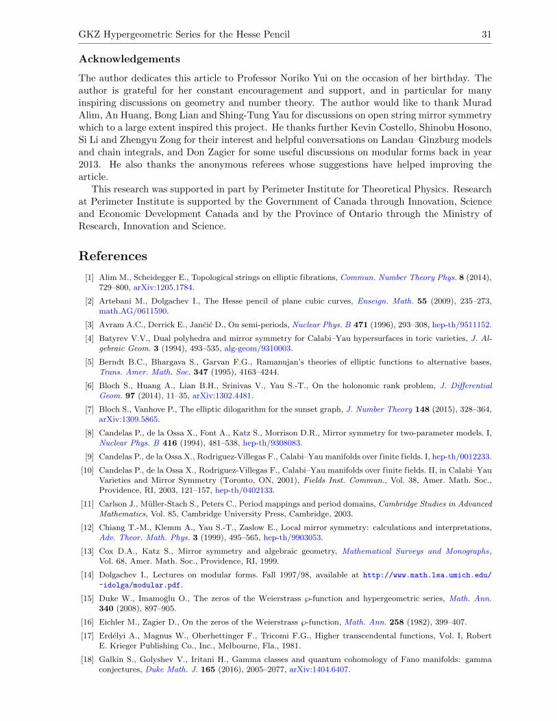
GKZ Hypergeometric Series for the Hesse Pencil 31
Acknowledgements
The author dedicates this article to Professor Noriko Yui on the occasion of her birthday. Theauthor is grateful for her constant encouragement and support, and in particular for manyinspiring discussions on geometry and number theory. The author would like to thank MuradAlim, An Huang, Bong Lian and Shing-Tung Yau for discussions on open string mirror symmetrywhich to a large extent inspired this project. He thanks further Kevin Costello, Shinobu Hosono,Si Li and Zhengyu Zong for their interest and helpful conversations on Landau–Ginzburg modelsand chain integrals, and Don Zagier for some useful discussions on modular forms back in year2013. He also thanks the anonymous referees whose suggestions have helped improving thearticle.
This research was supported in part by Perimeter Institute for Theoretical Physics. Researchat Perimeter Institute is supported by the Government of Canada through Innovation, Scienceand Economic Development Canada and by the Province of Ontario through the Ministry ofResearch, Innovation and Science.
References
[1] Alim M., Scheidegger E., Topological strings on elliptic fibrations, Commun. Number Theory Phys. 8 (2014),729–800, arXiv:1205.1784.
[2] Artebani M., Dolgachev I., The Hesse pencil of plane cubic curves, Enseign. Math. 55 (2009), 235–273,math.AG/0611590.
[3] Avram A.C., Derrick E., Jancic D., On semi-periods, Nuclear Phys. B 471 (1996), 293–308, hep-th/9511152.
[4] Batyrev V.V., Dual polyhedra and mirror symmetry for Calabi–Yau hypersurfaces in toric varieties, J. Al-gebraic Geom. 3 (1994), 493–535, alg-geom/9310003.
[5] Berndt B.C., Bhargava S., Garvan F.G., Ramanujan’s theories of elliptic functions to alternative bases,Trans. Amer. Math. Soc. 347 (1995), 4163–4244.
[6] Bloch S., Huang A., Lian B.H., Srinivas V., Yau S.-T., On the holonomic rank problem, J. DifferentialGeom. 97 (2014), 11–35, arXiv:1302.4481.
[7] Bloch S., Vanhove P., The elliptic dilogarithm for the sunset graph, J. Number Theory 148 (2015), 328–364,arXiv:1309.5865.
[8] Candelas P., de la Ossa X., Font A., Katz S., Morrison D.R., Mirror symmetry for two-parameter models. I,Nuclear Phys. B 416 (1994), 481–538, hep-th/9308083.
[9] Candelas P., de la Ossa X., Rodriguez-Villegas F., Calabi–Yau manifolds over finite fields. I, hep-th/0012233.
[10] Candelas P., de la Ossa X., Rodriguez-Villegas F., Calabi–Yau manifolds over finite fields. II, in Calabi–YauVarieties and Mirror Symmetry (Toronto, ON, 2001), Fields Inst. Commun., Vol. 38, Amer. Math. Soc.,Providence, RI, 2003, 121–157, hep-th/0402133.
[11] Carlson J., Muller-Stach S., Peters C., Period mappings and period domains, Cambridge Studies in AdvancedMathematics, Vol. 85, Cambridge University Press, Cambridge, 2003.
[12] Chiang T.-M., Klemm A., Yau S.-T., Zaslow E., Local mirror symmetry: calculations and interpretations,Adv. Theor. Math. Phys. 3 (1999), 495–565, hep-th/9903053.
[13] Cox D.A., Katz S., Mirror symmetry and algebraic geometry, Mathematical Surveys and Monographs,Vol. 68, Amer. Math. Soc., Providence, RI, 1999.
[14] Dolgachev I., Lectures on modular forms. Fall 1997/98, available at http://www.math.lsa.umich.edu/
~idolga/modular.pdf.
[15] Duke W., Imamoglu O., The zeros of the Weierstrass ℘-function and hypergeometric series, Math. Ann.340 (2008), 897–905.
[16] Eichler M., Zagier D., On the zeros of the Weierstrass ℘-function, Math. Ann. 258 (1982), 399–407.
[17] Erdelyi A., Magnus W., Oberhettinger F., Tricomi F.G., Higher transcendental functions, Vol. I, RobertE. Krieger Publishing Co., Inc., Melbourne, Fla., 1981.
[18] Galkin S., Golyshev V., Iritani H., Gamma classes and quantum cohomology of Fano manifolds: gammaconjectures, Duke Math. J. 165 (2016), 2005–2077, arXiv:1404.6407.
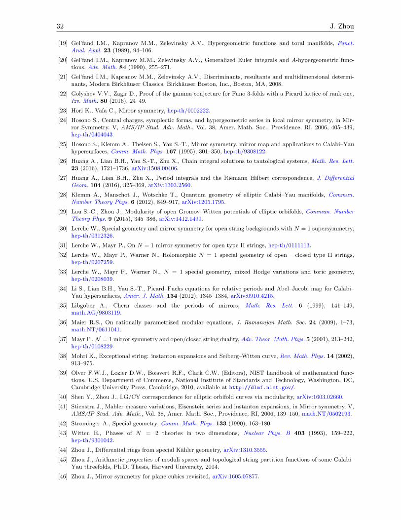
32 J. Zhou
[19] Gel’fand I.M., Kapranov M.M., Zelevinsky A.V., Hypergeometric functions and toral manifolds, Funct.Anal. Appl. 23 (1989), 94–106.
[20] Gel’fand I.M., Kapranov M.M., Zelevinsky A.V., Generalized Euler integrals and A-hypergeometric func-tions, Adv. Math. 84 (1990), 255–271.
[21] Gel’fand I.M., Kapranov M.M., Zelevinsky A.V., Discriminants, resultants and multidimensional determi-nants, Modern Birkhauser Classics, Birkhauser Boston, Inc., Boston, MA, 2008.
[22] Golyshev V.V., Zagir D., Proof of the gamma conjecture for Fano 3-folds with a Picard lattice of rank one,Izv. Math. 80 (2016), 24–49.
[23] Hori K., Vafa C., Mirror symmetry, hep-th/0002222.
[24] Hosono S., Central charges, symplectic forms, and hypergeometric series in local mirror symmetry, in Mir-ror Symmetry. V, AMS/IP Stud. Adv. Math., Vol. 38, Amer. Math. Soc., Providence, RI, 2006, 405–439,hep-th/0404043.
[25] Hosono S., Klemm A., Theisen S., Yau S.-T., Mirror symmetry, mirror map and applications to Calabi–Yauhypersurfaces, Comm. Math. Phys. 167 (1995), 301–350, hep-th/9308122.
[26] Huang A., Lian B.H., Yau S.-T., Zhu X., Chain integral solutions to tautological systems, Math. Res. Lett.23 (2016), 1721–1736, arXiv:1508.00406.
[27] Huang A., Lian B.H., Zhu X., Period integrals and the Riemann–Hilbert correspondence, J. DifferentialGeom. 104 (2016), 325–369, arXiv:1303.2560.
[28] Klemm A., Manschot J., Wotschke T., Quantum geometry of elliptic Calabi–Yau manifolds, Commun.Number Theory Phys. 6 (2012), 849–917, arXiv:1205.1795.
[29] Lau S.-C., Zhou J., Modularity of open Gromov–Witten potentials of elliptic orbifolds, Commun. NumberTheory Phys. 9 (2015), 345–386, arXiv:1412.1499.
[30] Lerche W., Special geometry and mirror symmetry for open string backgrounds with N = 1 supersymmetry,hep-th/0312326.
[31] Lerche W., Mayr P., On N = 1 mirror symmetry for open type II strings, hep-th/0111113.
[32] Lerche W., Mayr P., Warner N., Holomorphic N = 1 special geometry of open – closed type II strings,hep-th/0207259.
[33] Lerche W., Mayr P., Warner N., N = 1 special geometry, mixed Hodge variations and toric geometry,hep-th/0208039.
[34] Li S., Lian B.H., Yau S.-T., Picard–Fuchs equations for relative periods and Abel–Jacobi map for Calabi–Yau hypersurfaces, Amer. J. Math. 134 (2012), 1345–1384, arXiv:0910.4215.
[35] Libgober A., Chern classes and the periods of mirrors, Math. Res. Lett. 6 (1999), 141–149,math.AG/9803119.
[36] Maier R.S., On rationally parametrized modular equations, J. Ramanujan Math. Soc. 24 (2009), 1–73,math.NT/0611041.
[37] Mayr P., N = 1 mirror symmetry and open/closed string duality, Adv. Theor. Math. Phys. 5 (2001), 213–242,hep-th/0108229.
[38] Mohri K., Exceptional string: instanton expansions and Seiberg–Witten curve, Rev. Math. Phys. 14 (2002),913–975.
[39] Olver F.W.J., Lozier D.W., Boisvert R.F., Clark C.W. (Editors), NIST handbook of mathematical func-tions, U.S. Department of Commerce, National Institute of Standards and Technology, Washington, DC,Cambridge University Press, Cambridge, 2010, available at http://dlmf.nist.gov/.
[40] Shen Y., Zhou J., LG/CY correspondence for elliptic orbifold curves via modularity, arXiv:1603.02660.
[41] Stienstra J., Mahler measure variations, Eisenstein series and instanton expansions, in Mirror symmetry. V,AMS/IP Stud. Adv. Math., Vol. 38, Amer. Math. Soc., Providence, RI, 2006, 139–150, math.NT/0502193.
[42] Strominger A., Special geometry, Comm. Math. Phys. 133 (1990), 163–180.
[43] Witten E., Phases of N = 2 theories in two dimensions, Nuclear Phys. B 403 (1993), 159–222,hep-th/9301042.
[44] Zhou J., Differential rings from special Kahler geometry, arXiv:1310.3555.
[45] Zhou J., Arithmetic properties of moduli spaces and topological string partition functions of some Calabi–Yau threefolds, Ph.D. Thesis, Harvard University, 2014.
[46] Zhou J., Mirror symmetry for plane cubics revisited, arXiv:1605.07877.