APV and WACC Capital Structure with Taxes: Lecture 19faculty.som.yale.edu/zhiwuchen/finance-core/slides/l19...3 Capital Structure with Taxes With taxes, cash flows now split into 3

U.C. Berkeley© M. Spiegel and R. Stanton, 2000 1

Lecture 19Capital Structure with Taxes:

APV and WACC

Lecture 19Capital Structure with Taxes:

APV and WACC

■ Readings:– BM, Chapter 19– Reader, Lecture 19


Where are we so far?Where are we so far?

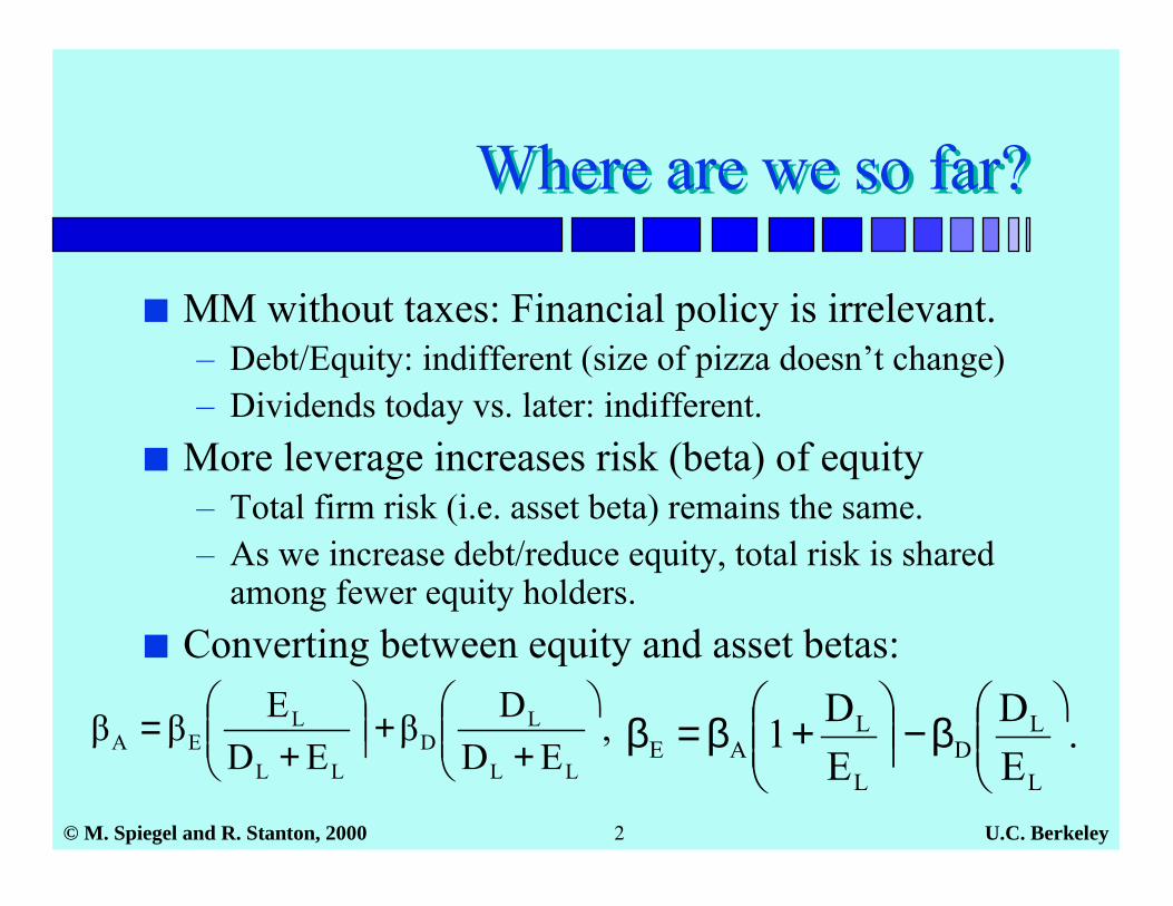
■ MM without taxes: Financial policy is irrelevant.– Debt/Equity: indifferent (size of pizza doesn’t change)– Dividends today vs. later: indifferent.

■ More leverage increases risk (beta) of equity– Total firm risk (i.e. asset beta) remains the same.– As we increase debt/reduce equity, total risk is shared

among fewer equity holders.■ Converting between equity and asset betas:

,ED

DβED

EββLL

LD

LL

LEA

��

�

++��

��

�

+= .

ED

ED1

L

LD

L

LAE

��

�β−��

��

�+β=β


Capital Structure with TaxesCapital Structure with Taxes

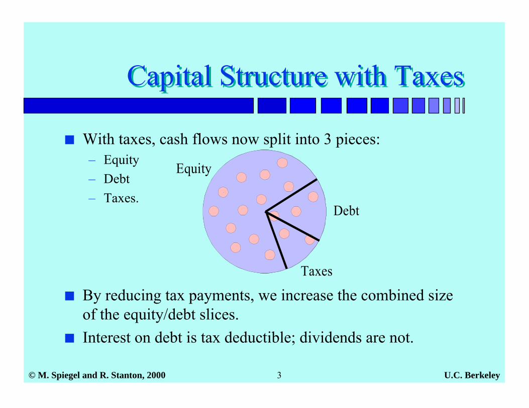
■ With taxes, cash flows now split into 3 pieces:– Equity– Debt– Taxes.

Equity

Debt

Taxes

■ By reducing tax payments, we increase the combined sizeof the equity/debt slices.

■ Interest on debt is tax deductible; dividends are not.


Example of Tax Benefit ofInterest Payments on DebtExample of Tax Benefit ofInterest Payments on Debt

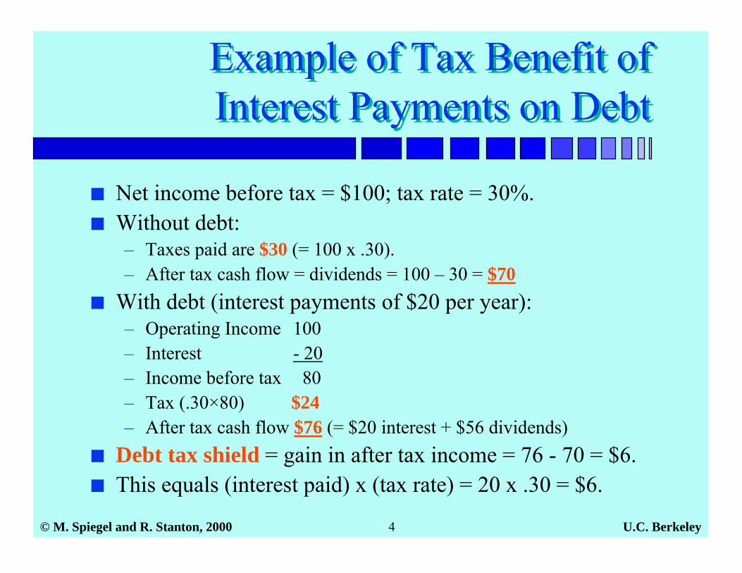
■ Net income before tax = $100; tax rate = 30%.■ Without debt:

– Taxes paid are $30 (= 100 x .30).– After tax cash flow = dividends = 100 – 30 = $70

■ With debt (interest payments of $20 per year):– Operating Income 100– Interest - 20– Income before tax 80– Tax (.30×80) $24– After tax cash flow $76 (= $20 interest + $56 dividends)

■ Debt tax shield = gain in after tax income = 76 - 70 = $6.■ This equals (interest paid) x (tax rate) = 20 x .30 = $6.


Valuation with TaxesValuation with Taxes

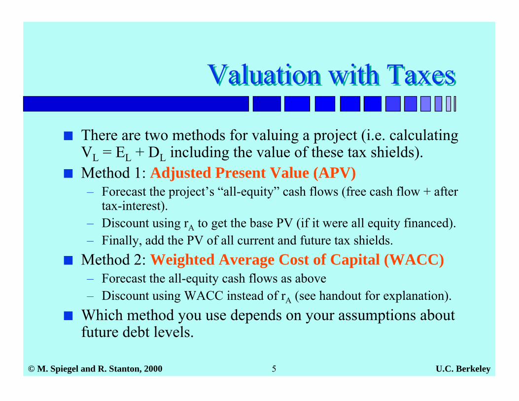
■ There are two methods for valuing a project (i.e. calculatingVL = EL + DL including the value of these tax shields).

■ Method 1: Adjusted Present Value (APV)– Forecast the project’s “all-equity” cash flows (free cash flow + after

tax-interest).– Discount using rA to get the base PV (if it were all equity financed).– Finally, add the PV of all current and future tax shields.

■ Method 2: Weighted Average Cost of Capital (WACC)– Forecast the all-equity cash flows as above– Discount using WACC instead of rA (see handout for explanation).

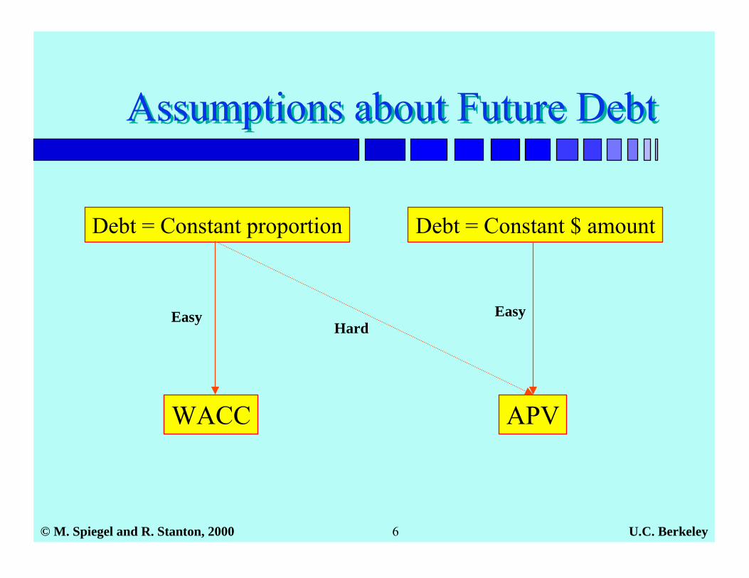
■ Which method you use depends on your assumptions aboutfuture debt levels.


Assumptions about Future DebtAssumptions about Future Debt

Debt = Constant $ amountDebt = Constant proportion

WACC

Easy

APV

EasyHard


Converting between Equity betasand Asset betas (with Taxes)

Converting between Equity betasand Asset betas (with Taxes)

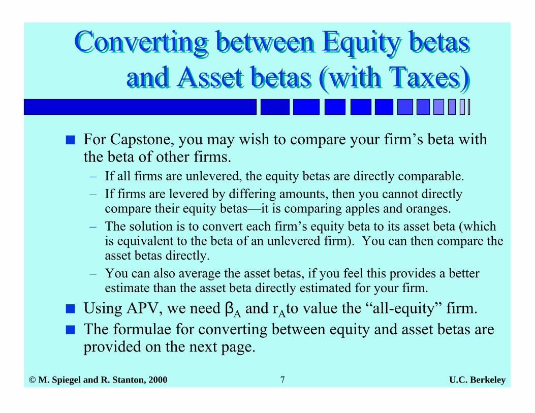
■ For Capstone, you may wish to compare your firm’s beta withthe beta of other firms.– If all firms are unlevered, the equity betas are directly comparable.– If firms are levered by differing amounts, then you cannot directly

compare their equity betas—it is comparing apples and oranges.– The solution is to convert each firm’s equity beta to its asset beta (which

is equivalent to the beta of an unlevered firm). You can then compare theasset betas directly.

– You can also average the asset betas, if you feel this provides a betterestimate than the asset beta directly estimated for your firm.

■ Using APV, we need βA and rAto value the “all-equity” firm.■ The formulae for converting between equity and asset betas are

provided on the next page.


Converting between Equity andAsset Betas

Converting between Equity andAsset Betas

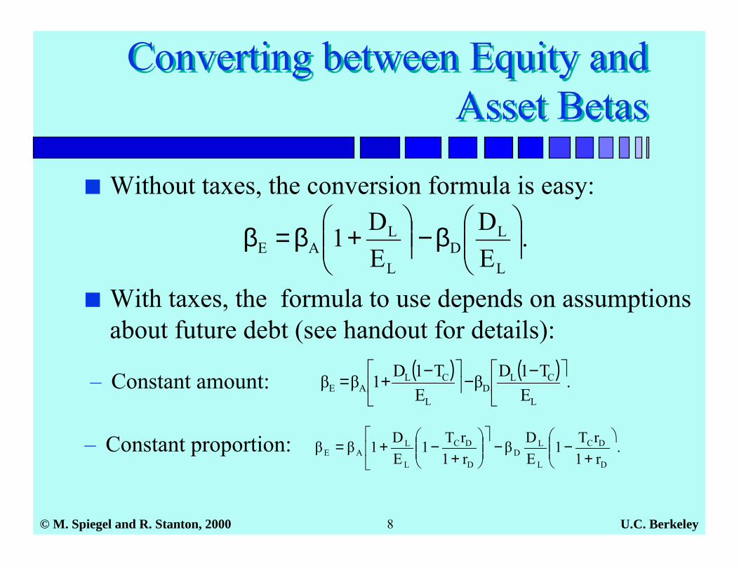
■ Without taxes, the conversion formula is easy:

■ With taxes, the formula to use depends on assumptionsabout future debt (see handout for details):

– Constant amount: ( ) ( ) .E

T1DβE

T1D1ββL

CLD

L

CLAE

��

� −−��

��

� −+=

.r1rT1

EDβ

r1rT1

ED1ββ

D

DC

L

LD

D

DC

L

LAE

��

�

+−−

��

�

��

�

+−+=– Constant proportion:

.ED

ED1

L

LD

L

LAE ��

��

�β−��

��

�+β=β


Valuation using APVValuation using APV

■ Adjusted Present Value (APV):– APV = Base PV (with all equity financing) + PV of all

tax shields.

■ APV is easiest to use when we assume a constantamount of debt forever, but can be used in othercases with enough effort.– WACC requires a constant proportion of debt

forever. It cannot be used otherwise.


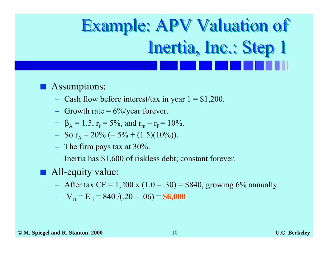
Example: APV Valuation ofInertia, Inc.: Step 1

Example: APV Valuation ofInertia, Inc.: Step 1

■ Assumptions:– Cash flow before interest/tax in year 1 = $1,200.– Growth rate = 6%/year forever.− βA = 1.5, rf = 5%, and rm – rf = 10%.– So rA = 20% (= 5% + (1.5)(10%)).– The firm pays tax at 30%.– Inertia has $1,600 of riskless debt; constant forever.

■ All-equity value:– After tax CF = 1,200 x (1.0 – .30) = $840, growing 6% annually.– VU = EU = 840 /(.20 – .06) = $6,000


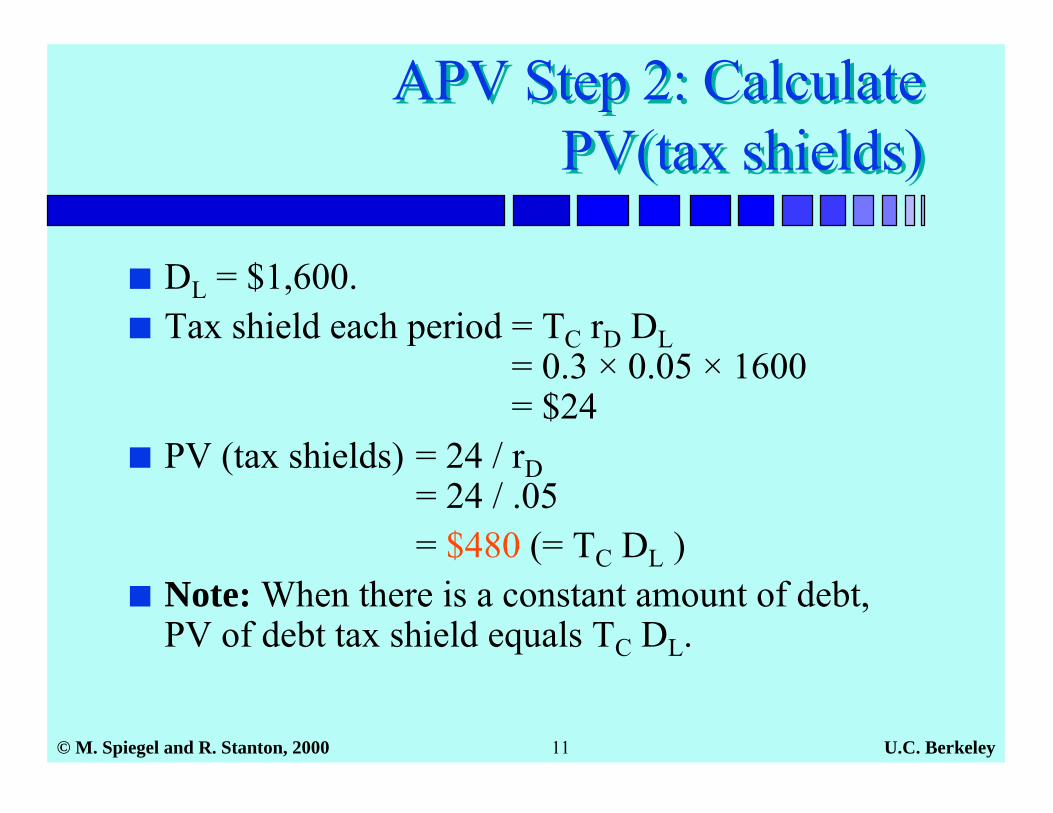
APV Step 2: CalculatePV(tax shields)

APV Step 2: CalculatePV(tax shields)

■ DL = $1,600.■ Tax shield each period = TC rD DL

= 0.3 × 0.05 × 1600= $24

■ PV (tax shields) = 24 / rD= 24 / .05

= $480 (= TC DL )■ Note: When there is a constant amount of debt,

PV of debt tax shield equals TC DL.


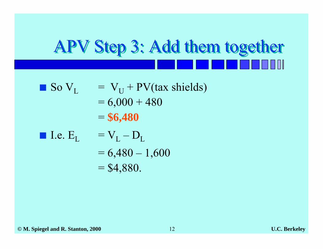
APV Step 3: Add them togetherAPV Step 3: Add them together

■ So VL = VU + PV(tax shields)= 6,000 + 480= $6,480

■ I.e. EL = VL – DL

= 6,480 – 1,600= $4,880.


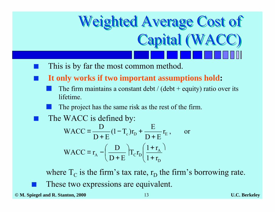
Weighted Average Cost ofCapital (WACC)

Weighted Average Cost ofCapital (WACC)

■ This is by far the most common method.■ It only works if two important assumptions hold:

■ The firm maintains a constant debt / (debt + equity) ratio over itslifetime.

■ The project has the same risk as the rest of the firm.

■ The WACC is defined by:

��

�

++

��

��

�

+−=

++−

+=

D

ADCA

EDc

r1r1rT

EDDrWACC

or,rED

Er)T1(ED

DWACC

where TC is the firm’s tax rate, rD the firm’s borrowing rate.■ These two expressions are equivalent.


Example: WACC Valuation ofDynamic Cities: Step 1

Example: WACC Valuation ofDynamic Cities: Step 1

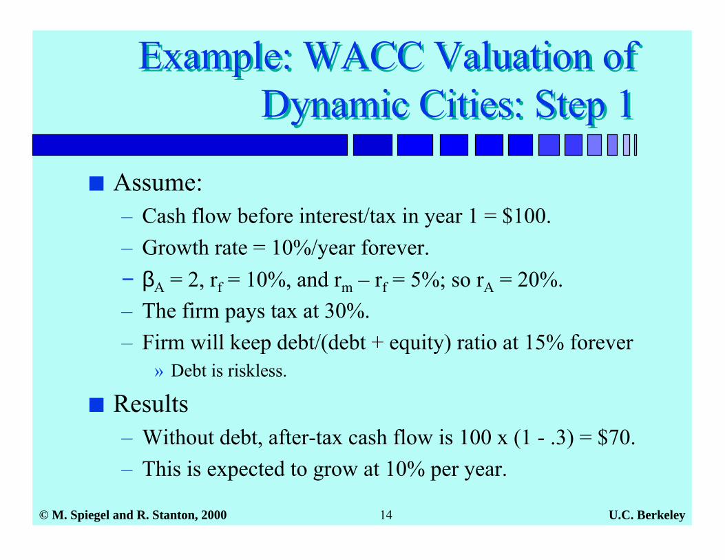
■ Assume:– Cash flow before interest/tax in year 1 = $100.– Growth rate = 10%/year forever.− βA = 2, rf = 10%, and rm – rf = 5%; so rA = 20%.– The firm pays tax at 30%.– Firm will keep debt/(debt + equity) ratio at 15% forever

» Debt is riskless.

■ Results– Without debt, after-tax cash flow is 100 x (1 - .3) = $70.– This is expected to grow at 10% per year.


WACC step 2: Calculate WACCWACC step 2: Calculate WACC

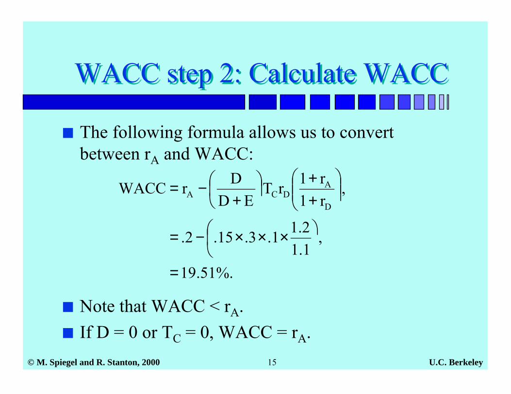
■ The following formula allows us to convertbetween rA and WACC:

%.51.19

,1.12.11.3.15.2.

,r1r1rT

EDDrWACC

D

ADCA

=

��

� ×××−=

��

��

�

++

��

��

�

+−=

■ Note that WACC < rA.■ If D = 0 or TC = 0, WACC = rA.


WACC step 3: Discount all-equity cash flows using WACC

WACC step 3: Discount all-equity cash flows using WACC

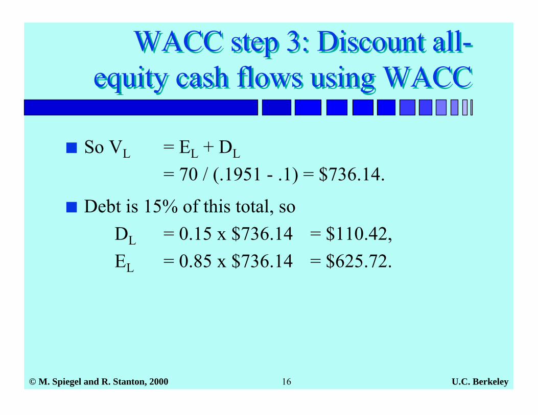
■ So VL = EL + DL

= 70 / (.1951 - .1) = $736.14.

■ Debt is 15% of this total, soDL = 0.15 x $736.14 = $110.42,EL = 0.85 x $736.14 = $625.72.


Valuation on one slide…Valuation on one slide…

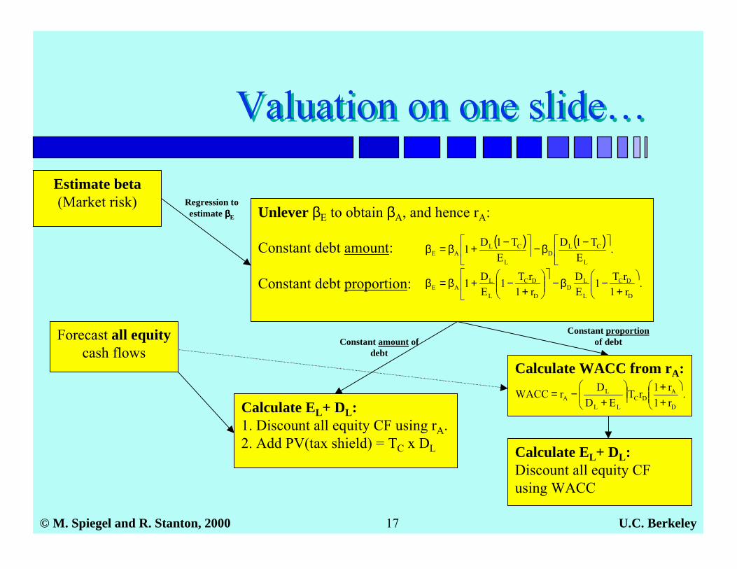
Estimate beta(Market risk)

Forecast all equitycash flows

Calculate EL+ DL:1. Discount all equity CF using rA.2. Add PV(tax shield) = TC x DL

Constant amount ofdebt

Regression toestimate ββββE Unlever βE to obtain βA, and hence rA:

Constant debt amount:

Constant debt proportion: .r1rT1

ED

r1rT1

ED1

D

DC

L

LD

D

DC

L

LAE

��

�

+−β−

��

�

��

�

+−+β=β

( ) ( ) .E

T1DE

T1D1L

CLD

L

CLAE

��

� −β−��

��

� −+β=β

Calculate EL+ DL:Discount all equity CFusing WACC

Constant proportionof debt

Calculate WACC from rA:.

r1r1rT

EDDrWACC

D

ADC

LL

LA

��

�

++

��

��

�

+−=


WACC vs. APVWACC vs. APV

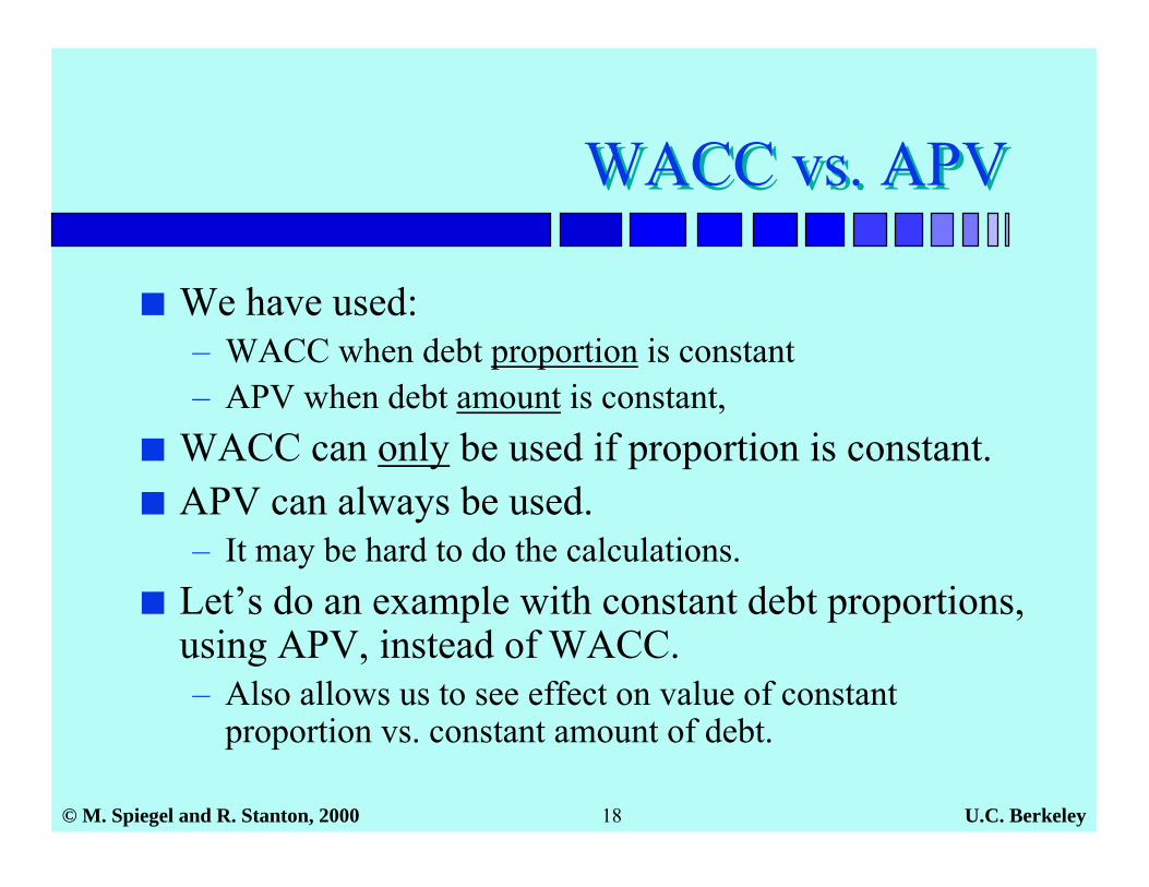
■ We have used:– WACC when debt proportion is constant– APV when debt amount is constant,

■ WACC can only be used if proportion is constant.■ APV can always be used.

– It may be hard to do the calculations.■ Let’s do an example with constant debt proportions,

using APV, instead of WACC.– Also allows us to see effect on value of constant

proportion vs. constant amount of debt.


Constant amount vs. constantproportion of debt


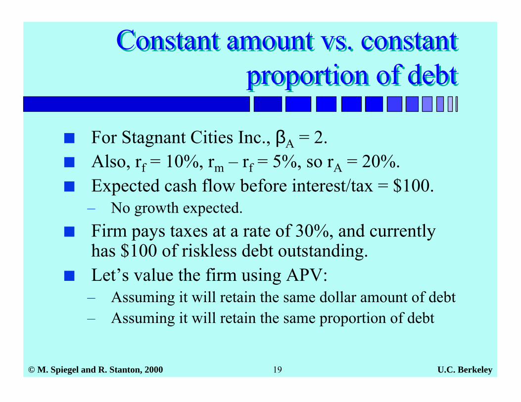
■ For Stagnant Cities Inc., βA = 2.■ Also, rf = 10%, rm – rf = 5%, so rA = 20%.■ Expected cash flow before interest/tax = $100.

– No growth expected.■ Firm pays taxes at a rate of 30%, and currently

has $100 of riskless debt outstanding.■ Let’s value the firm using APV:

– Assuming it will retain the same dollar amount of debt– Assuming it will retain the same proportion of debt


Valuing Stagnant Cities withconstant amount of debt

Valuing Stagnant Cities withconstant amount of debt

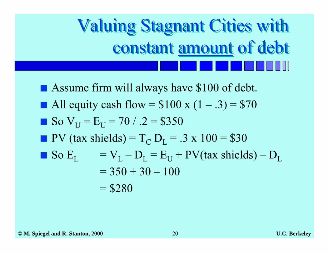
■ Assume firm will always have $100 of debt.■ All equity cash flow = $100 x (1 – .3) = $70■ So VU = EU = 70 / .2 = $350■ PV (tax shields) = TC DL = .3 x 100 = $30■ So EL = VL – DL = EU + PV(tax shields) – DL

= 350 + 30 – 100 = $280


Valuing Stagnant Cities withconstant proportion of debt


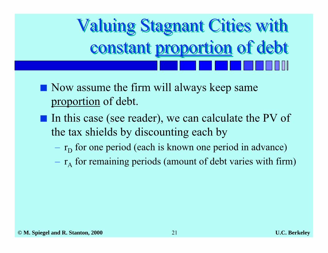
■ Now assume the firm will always keep sameproportion of debt.

■ In this case (see reader), we can calculate the PV ofthe tax shields by discounting each by– rD for one period (each is known one period in advance)– rA for remaining periods (amount of debt varies with firm)




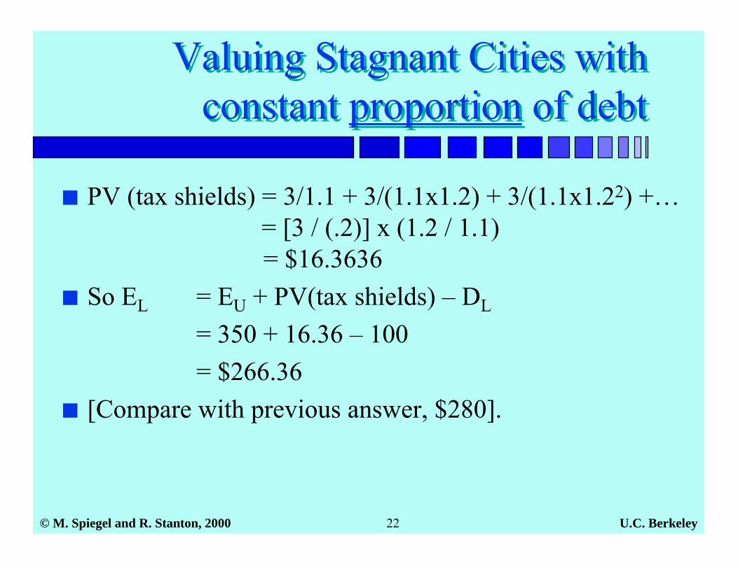
■ PV (tax shields) = 3/1.1 + 3/(1.1x1.2) + 3/(1.1x1.22) +… = [3 / (.2)] x (1.2 / 1.1)

= $16.3636■ So EL = EU + PV(tax shields) – DL

= 350 + 16.36 – 100 = $266.36■ [Compare with previous answer, $280].




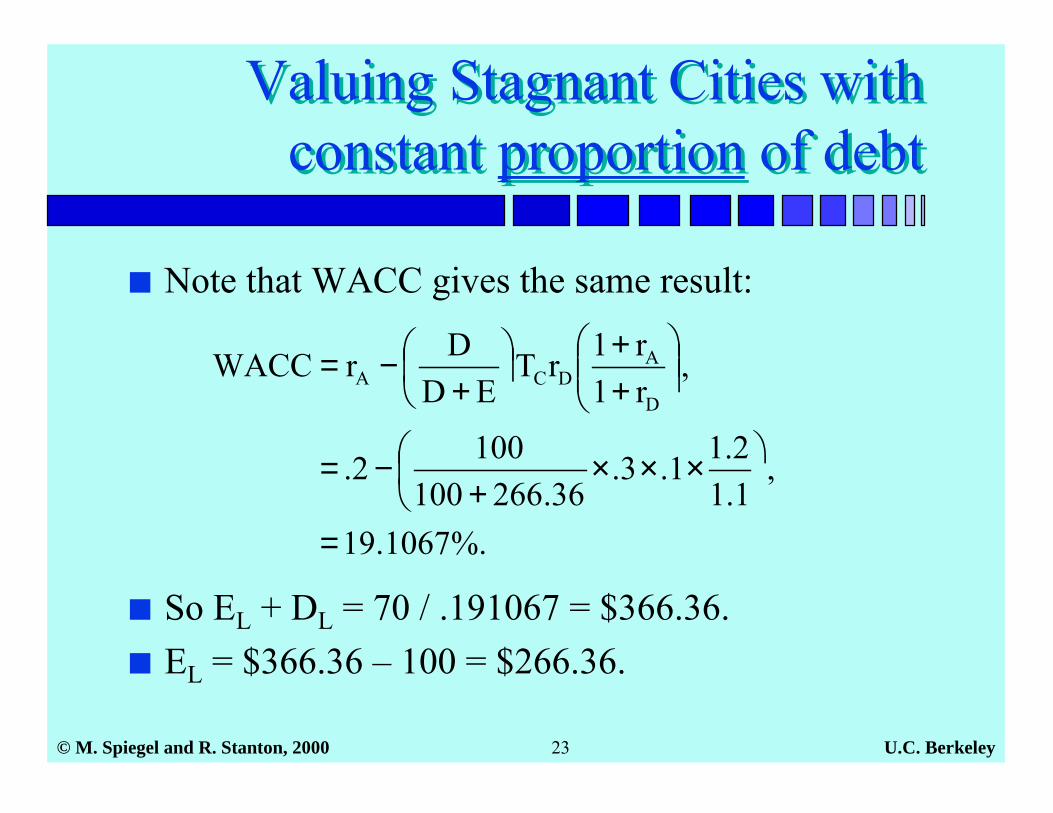
■ Note that WACC gives the same result:

%.1067.19

,1.12.11.3.

36.2661001002.

,r1r1rT

EDDrWACC

D

ADCA

=

��

� ×××+

−=

��

��

�

++

��

��

�

+−=

■ So EL + DL = 70 / .191067 = $366.36.■ EL = $366.36 – 100 = $266.36.




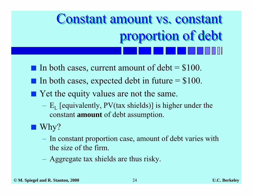
■ In both cases, current amount of debt = $100.■ In both cases, expected debt in future = $100.■ Yet the equity values are not the same.

– EL [equivalently, PV(tax shields)] is higher under theconstant amount of debt assumption.

■ Why?– In constant proportion case, amount of debt varies with

the size of the firm.– Aggregate tax shields are thus risky.


Using WACC given an initialamount of debt

Using WACC given an initialamount of debt

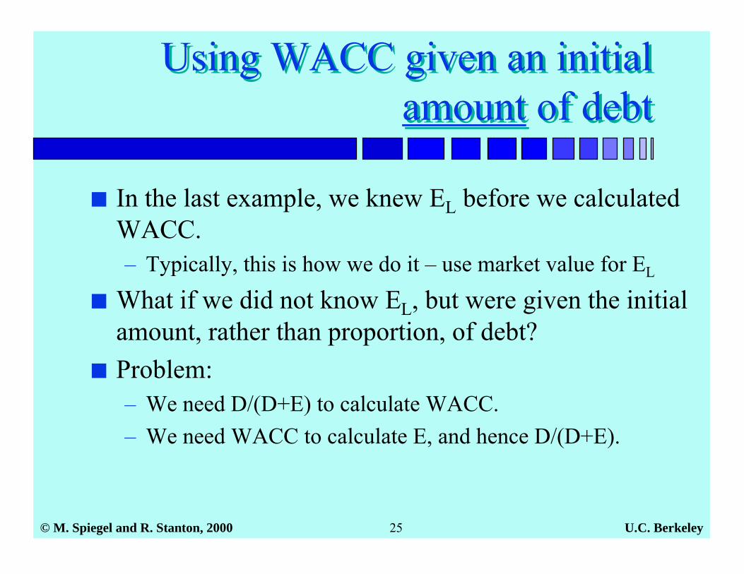
■ In the last example, we knew EL before we calculatedWACC.– Typically, this is how we do it – use market value for EL

■ What if we did not know EL, but were given the initialamount, rather than proportion, of debt?

■ Problem:– We need D/(D+E) to calculate WACC.– We need WACC to calculate E, and hence D/(D+E).


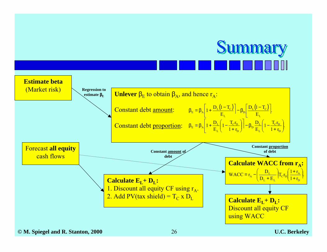
SummarySummary

Estimate beta(Market risk)

Forecast all equitycash flows

Calculate EL+ DL:1. Discount all equity CF using rA.2. Add PV(tax shield) = TC x DL

Constant amount ofdebt

Regression toestimate ββββE Unlever βE to obtain βA, and hence rA:

Constant debt amount:

Constant debt proportion: .r1rT1

ED

r1rT1

ED1

D

DC

L

LD

D

DC

L

LAE

��

�

+−β−�

��

�

��

�

+−+β=β

( ) ( ) .E

T1DE

T1D1L

CLD

L

CLAE �

��

� −β−��

��

� −+β=β

Calculate EL+ DL:Discount all equity CFusing WACC

Constant proportionof debt

Calculate WACC from rA:.

r1r1rT

EDDrWACC

D

ADC

LL

LA ��

��

�

++

��

��

�

+−=

Documents

APV and WACC Capital Structure with Taxes: Lecture 19faculty.som.yale.edu/zhiwuchen/finance-core/slides/l19...3 Capital Structure with Taxes With taxes, cash flows now split into 3