CAPITAL BUDGETING, VALUATION AND PERSONAL TAXES

by

Ian M Dobbs

and

Anthony D Miller*

KEYWORDS: Capital Budgeting, Valuation, Value Additivity, Discounting, Personal

Taxes.

JEL CLASSIFICATION: G12, G31, G32

* The authors are, respectively, Reader in Business Economics and Finance, and Lecturer in Accounting and Financial Management in the Department of Accounting and Finance, University of Newcastle Upon Tyne.

2 Abstract

This paper examines the relationship between before tax and after tax valuation and uses this to

examine the literature on capital budgeting and capital structure in the presence of corporate and

personal taxes, a literature which features a bewildering array of valuation formulae. Some of

the variation between such formulae naturally arises out of variations in underlying model

assumptions; however, in several cases, it arises because there are (by no means obvious)

internal inconsistencies. The potential magnitude of the errors that might arise in a capital

budgeting context is then explored through sensitivity analysis.

I. Introduction and Review of the Literature For many years the Value Additivity Principle (VAP) has provided the cornerstone for

the valuation of complex assets within a setting of perfect capital markets. Under this

principle, a portfolio can be correctly valued by breaking it into its constituent assets,

independently valuing each asset, and then adding the resulting values together (Haley &

Schall [1973]). Applied to the theory of capital structure1, where the focus is on the

interaction between an investment decision and its financing, the VAP prescribes that the

value of a levered investment should be equal to the value of an otherwise-identical

unlevered investment plus the value of incremental cash flows attributable to leverage.

Modigliani & Miller [1963] presented a seminal model in which debt created a valuable

incremental corporation tax shield. In addition to assigning a value to this tax shield,

Modigliani and Miller (MM) derived an adjusted discount rate (ADR) which could be

used to compute the value of a levered investment without explicit consideration of the

incremental cash flows arising from leverage. This ADR subsequently found a place in

conventional textbook accounts of capital budgeting procedures as the weighted average

cost of capital (e.g. Brealey and Myers [1996], Buckley et al. [1998]). MM’s specific

results, however, were based upon a number of restrictive assumptions, including (a) that

there are no personal taxes, (b) that operating cash flows conform to a specific and

permanent stable pattern, and (c) that the level of debt is fixed and permanent.

The work of MM was subsequently generalised in a number of different ways. Miller

[1977] and DeAngelo and Masulis [1980] discussed the value of corporation tax shields

in a world with personal taxation, whilst Miles & Ezzell [1980], retaining the assumption

1 For a useful survey of capital structure research outside the perfect capital markets setting, see Harris & Raviv [1991].

4

of no personal taxation, derived an ADR for any pattern of operating cash flows. Strictly

speaking, the Miles-Ezzell result is not a full generalisation of MM's earlier result,

because the Miles-Ezzell financing policy, a so-called Active Debt Management Policy

(ADMP), and the MM financing policy, assumption (c) above, are in general mutually

conflicting.2 Concurrent with the above developments were attempts to integrate the

Capital Asset Pricing Model (CAPM) of Sharpe [1964], Lintner [1965] and Mossin

[1966] with MM's model of capital structure.3 This raised interesting issues for multi-

period capital budgeting, for as well as the MM restrictions outlined above, use of the 1-

period CAPM implied further, and possibly contradictory, restrictions.4

Following this early work, researchers have striven to synthesize these various strands

with the objective of furnishing a realistic yet practical approach to capital budgeting

and, in particular, the valuation of arbitrary risky multi-period cash flows. Clubb &

Doran [1991, 1992], Appleyard & Strong [1989], Strong & Appleyard [1992] and

Taggart [1991] all employ the Miles-Ezzell ADMP to derive formulae relevant to the

valuation of a levered asset with an arbitrary pattern of operating cash flows, and all

authors allow for non-zero personal taxes. Yet, despite the broadly common framework

adopted by these authors, inspection of their results reveals a bewildering variety of

valuation formula. This paper demonstrates that discrepancies and inconsistencies can

arise, and indeed, have arisen, in models which incorporate personal taxation. However,

before presenting a more formal analysis, the following stylised example may help to

2. Moreover, both financing policies were assumed merely for analytical convenience. Neither has normative force.

3. See, for example, Hamada[1972].

4. For example, the Sharpe-Lintner-Mossin CAPM was derived under an assumption that investors have a one-period investment horizon. Fama [1970, 1977] outlined sufficient conditions for the validity of this one-period CAPM in a multi-period investment context. See also Merton [1973] for a discussion of the same issue in a continuous time setting.

5

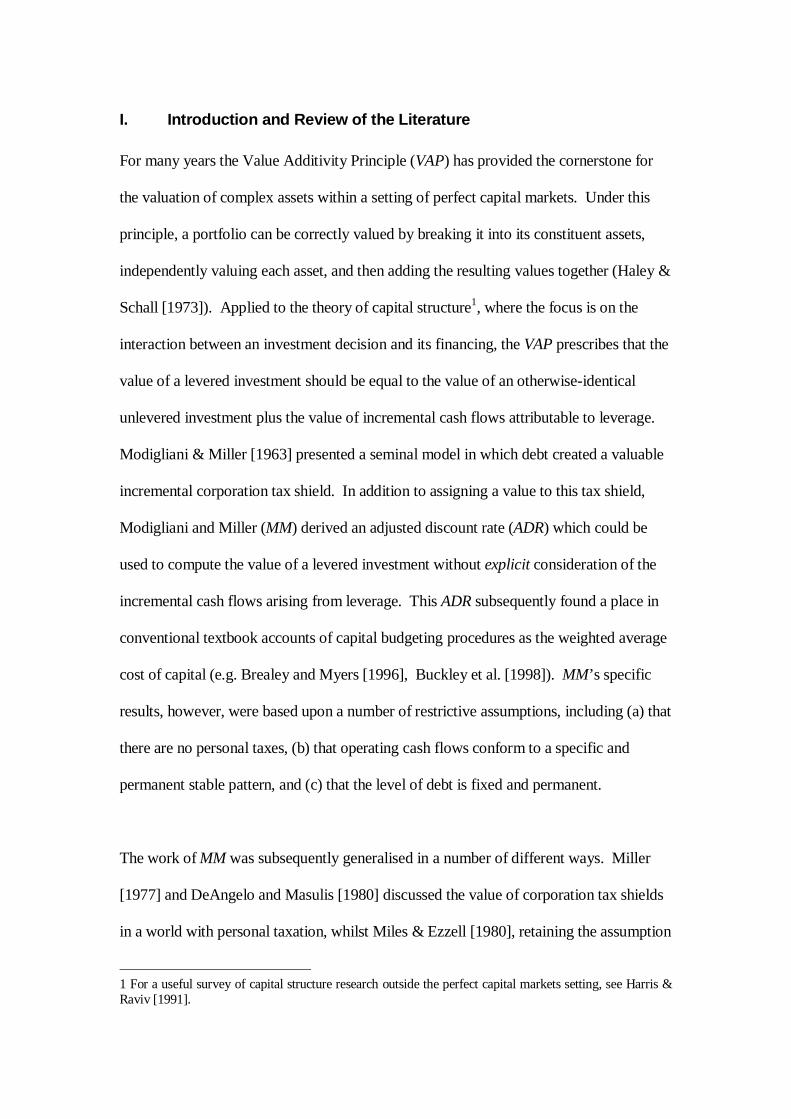
clarify what is at issue with the conventional valuation procedures used in some of the

capital budgeting and valuation literature.

Consider a risky cash flow which will be received next period. Suppose its current

expected value is £100 before personal taxes (BT) and, say, £95 after personal taxes

(AT). Given these figures, the implied effective tax rate is 5%.5 Let the equilibrium

AT discount rate for cash flows belonging to this risk class be 10%. The conventional

method of valuation would compute the present value by discounting the expected AT

cash flow at the AT discount rate, giving a correct value (current market price) for this

cash flow of £100(1-0.05)/1.1=£95/1.1=£86.3636. An alternative method of valuation

would specify an equilibrium risk-adjusted BT discount rate to be applied to the

expected BT cash flow. How should this rate be determined? In much of the above

literature, it is assumed that there is a well-defined relationship between the two kinds

of discount rate and the tax rate - namely, following Miller [1977], that

/(1 *)r ρ τ= − , (1)

where r is the equilibrium BT discount rate, ρ is the equilibrium AT discount rate and

*τ is the effective tax rate. This specification applied to the above numerical

example would give the BT rate as 0.1/(1 0.05) 0.10526r = − = and a value for the

cash flow of £100/1.10526 = £90.4762. The discrepancy between the AT valuation of

£86.3636 and the BT valuation of £90.4762 (an error of about 5%) clearly indicates

that the relationship encapsulated in equation (1) cannot be generally correct. In fact,

if the market value of the cash flow was indeed £86.3636 as indicated by the AT

5 For example, this would be the result if the marginal rate of income tax was 5% and the capital gains tax rate was zero. However, note that the details of the tax regime – and hence of how the effective tax on a cash flow arises - are of no importance in this paper – so long as there are some tax effects. The concern in this paper is purely with the problem of how to conduct consistent before- and after-tax valuation analysis.

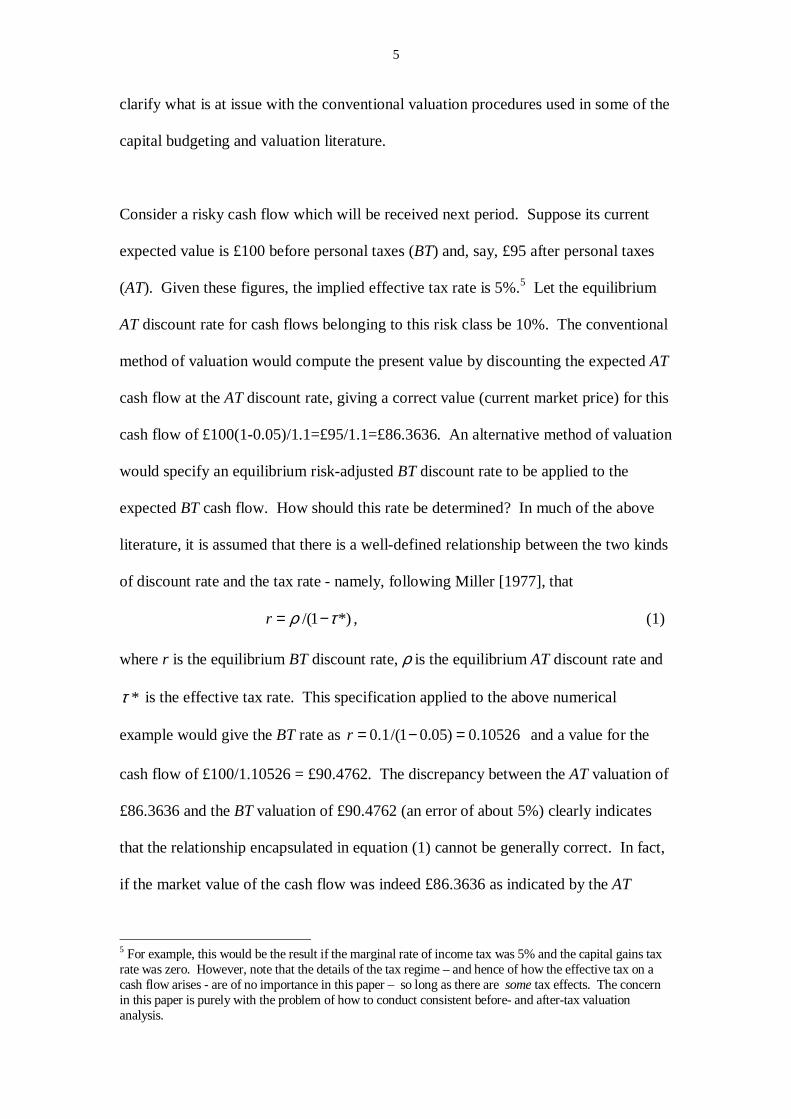
6

analysis, correct valuation using a BT discount rate r would require that this BT rate

be given by

100

86.3636 0.157891

rr

= � =+

.

Thus the correct BT discount rate is a whole five percentage points above the rate

calculated in (1).6 Furthermore, if the example is modified slightly by lengthening the

time before the cash flow will be received to two periods, with no other changes, then

its value (based on an AT analysis) is 2 2£100(1 0.05) /1.1 £95/1.1− = = £78.5124. If

£78.5124 is in fact the market value of the risky cash flow, the implicit value for the

BT rate r to give this answer is

( )2

10078.5214 0.12858

1r

r= � =

+,

a rate which differs from the period-1 BT rate calculated above. These calculations

thus demonstrate that the relationship between BT and AT rates and taxation is

generally more complex than implied by the simple ‘grossing up’ procedure in

equation (1) and that this relationship is affected by the time to maturity of the

expected cash flow. Note that these conclusions have been reached without any

assumption being made about the precise tax regime and despite the fact that the

parameters of the problem are held constant when time to maturity is lengthened.

The object of the present paper is to identify the relationship between before and after

personal tax discount rates and to show how the relationship is generally a non-linear

6 And of course, valuation errors associated with individual cash flows may also be magnified in an overall calculation of net present value. To illustrate, suppose the above effective tax rate (5%) and an AT discount rate of 10% apply and that a project involved an initial outlay of £90 (BT) to generate the above period one BT expected cash flow of £100. The correct net present value is thus £90-£86.3636=+£3.6364 whilst the AT valuation would be £90-£90.4762= -£0.4762. In this example, not only would the project be rejected on this incorrect calculation, but the valuation error would be over 100%.

7

function of the timing of the cash flow (as illustrated in the above numerical example).

Having done this, the paper then addresses the above literature to see to what extent it

deals adequately with these relationships - and hence whether or not the observed

differences in valuation formulae arise out of differences in assumptions - or simply out

of internal incoherence in model assumptions.

Section II sets out the basic framework which is then used to investigate the above

literature, generally referred to below as ‘ the surveyed works’ , which deals with

personal taxes. Specifically, section III focuses on the case of the level perpetuity (as

dealt with in Miller [1977]) whilst section IV deals with the literature concerned with

the valuation of arbitrary finite cash flows (Clubb & Doran [1991, 1992], Appleyard &

Strong [1989], Strong & Appleyard [1992] and Taggart [1991]). Section V then

examines the magnitude of the error implied if the simple ‘grossing up’ rule is used,

and section VI draws together the main conclusions.

II. Personal Taxes and Discount Factors The standard approach adopted in the literature to valuing an asset is to (a) estimate the

expected future cash flows the asset will generate, (b) specify a discount factor for each

of these cash flows, and (c), invoking the value additivity principle (VAP), sum the

discounted expected cash flows to obtain a single numerical value. However, when

taxation is charged at the personal level, it is possible to pursue a ‘before personal taxes’

calculation of value or an ‘after personal taxes’ calculation of value. That is,

(i) to work with the set of expected gross cash flows i.e. before personal

taxes have been deducted (BT), - and use BT discount rates in

performing the valuation calculation, or

(ii) to work with the set of expected net cash flows i.e. after personal taxes

have been deducted (AT) - and use AT discount rates.

8

Since the market value of any given investment is a unique number, it follows that, in a

given model, it should make no difference which approach is adopted. That is, starting

with a given set of BT (AT) project cash flows, calculating value using BT (AT) discount

rates should give the same value as that from first computing AT (BT) cash flows and

then computing value using the AT (BT) discount rates. Indeed this is such an important

a property, it is worth stating more formally.

Lemma 1: A necessary condition for the validity of using both the BT and AT valuation approaches within a model is that the two approaches must assign an identical market value to any given asset.

As will be seen shortly, Lemma 1 implies the existence of definite relationships between

the discount factors used in the BT and AT approaches to valuation.

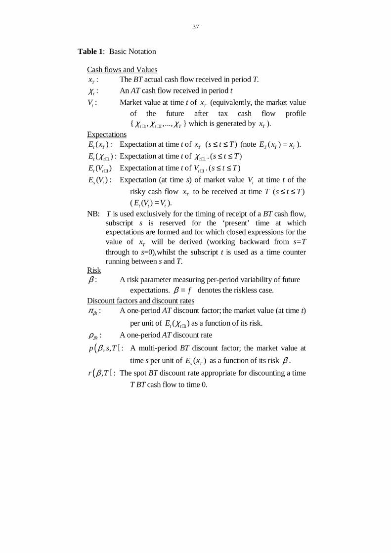
Table 1 about here (or earlier – but not later)

To proceed, focus upon the valuation of a single risky BT cash flow Tx 7 payable after T

periods. For convenience, table 1 gathers together a list of the principle notation used

in what follows. The analysis is more conveniently presented in terms of discount

factors rather than discount rates. However, given the results obtained for factors,

corresponding results in terms of discount rates can be obtained by using the

following definitional relationships:

( )( )

( ) 1/1,0, ( , ) ,0, 1

1 ( , )

T

Tp T r T p Tr T

β β ββ

−≡ � = −+

, (2)

7 Focusing upon a single cash flow involves no loss of generality for, given the VAP, it is permissible to value each individual cash flow out of a set of cash flows independently of the others in the set. Proposition 1, which follows, thus holds for each cash flow associated with a complex asset. Furthermore, analogous propositions might be developed for multiple cash flows considered jointly. See, for example, Proposition 2 below.

9

( )11/ 1

1t t tt

β β ββ

π ρ πρ

≡ � = −+

. (3)

The following assumptions are made:-

(A1) The rate of personal tax levied on Tx is τ and this is a constant over time and is payable without time lag.

(A2) Nominal capital gains/losses, whether realised or unrealised, are taxed at the rate of gτ , again constant over time and payable without time lag.

(A3) The per-period risk of ( )t TE x , 0 s t T≤ < ≤ , is known for certain and

constant over time (i.e. β is a constant).

(A4) ( )s TE x , ( 0 s T≤ ≤ ) is known for certain at time s, as are all tax rates and

discount factors. (A5) tβ βπ π= (∀β,∀t≥0).

(A6) 0 , 1gτ τ≤ < and 0 1fβπ π< < < .

These assumptions provide an analytical framework consistent with the surveyed

literature which deals with valuation in the presence of personal taxes. One can, of

course, debate whether the above assumptions provide a realistic or useful basis for

valuing assets. However, this lies outside the scope of the present paper, which is

concerned solely with capital budgeting and valuation within the framework already

established in the literature - and in particular with clarifying the extent to which the

above literature properly accounts for the implied relationship between BT and AT

discount factors. Nevertheless, some brief remarks concerning A1-A6 may be of

interest.

Assumptions A1, A3-A6 are explicit or trivially implicit in all of the surveyed works.

Assumption A4 is one of a set of sufficient conditions permitting use of the single-period

CAPM in a multi-period valuation context.8 Assumptions A1, A3 and A5 are standard

and widely used simplifying assumptions (see Fama [1977] and, especially, Myers &

8. For the other sufficient conditions, see Fama [1977].

10

Turnbull [1977]). A6 merely imposes that taxes are non-negative and less than 100%,

and that the risky discount rate is greater than a riskless one and that both are positive.

The main assumption used here which is less than obvious in the literature is A2.

This assumption entails that, for a single positive cash flow receivable at time T, there

will be a stream of CGT payments in each period prior to T, followed by a reclaim of

CGT at time T (since on payment of the cash flow, the market value of the asset falls

to zero, so there is a capital loss). Clubb and Doran [1992] explicitly make this

assumption, and in their [1991] paper, set gτ =0, so this is also consistent with A2 as a

special case. The remaining literature contains little discussion of taxation bases, but

in all cases there is an explicit assumption that there is an average or overall ‘equity

tax rate’ *τ which is constant over time for all assets (whatever their risk). It is

possible to show that a necessary and sufficient condition for this to be the case within

these models is that gτ τ= ; that is, the assumption of a constant effective equity tax

rate requires that dividend and CGT rates are equal and constant over time in these

models (the proof is given in appendix A1). Since the rate *τ >0 is applied to each

and every cash flow in a multi-period cash flow, this also entails our assumption A2,

namely that capital gains tax is payable on all changes in market value whether or not

capital gains are realised.9

9 As well as being necessary for modelling the surveyed work, this assumption, A2, is of interest in its own right because of its non-distortionary properties. By contrast, it is well known that, if CGT is payable only on realisation, this leads to ‘ lock in’ effects (the desire to hold appreciating assets to defer and so reduce the present value of CGT payments). Although tax authorities often limit the associated tax arbitrage opportunities by imposing loss-offset limits, these in turn distort investment choices away from more risky investments (Stiglitz[1969]). It is for these reasons that there are now arguments for introducing a mark-to-market form of CGT system (Shakow [1986]), and in a recent article, Auerbach [1991] develops an operational form for this.

11

What values the personal tax rates might take is naturally an empirical question,

although from a theoretical perspective, the relevant rates are those associated with

the ‘marginal investor’ (Miller [1977]).10 Given such rates can only be estimated, it is

often useful to study the sensitivity of valuation results to variation in such tax

parameters; this kind of analysis is conducted in section 5 below.

Under assumptions A1-A6, the relationship between BT and AT discount factors is

established in the following proposition:

Proposition 1: Assumptions A1-A6 imply the following necessary and sufficient condition for internally consistent valuation of any given BT risky cash flow Tx at any given time T; that the BT and AT discount factors must be related by the formula

( ) (1 )1,0,

1 (1 )

T

g

g f g

p T βττβ π

τ π τ

����� �−−= � � � �� � � �− −����� � .

Proof: See appendix A2

Writing

( ) ( ) ( ), 1 1g gk τ τ τ τ≡ − − , (4)

and

( ) (1 ),

(1 )g

f gf g

aτ

π τπ τ−

≡−

(5)

(and suppressing arguments for the functions k and a in what follows), the result can be

written more compactly as

( ) ( ),0,T

p T k a ββ π= . (6)

The full proof for Proposition 1 is completed in appendix A2. However, to get an

understanding for the processes involved, the first steps are detailed here. Given an

10 For the complications induced by tax clientele effects, see for example Elton and Gruber [1970], Miller and Scholes [1978], Litzenberger and Ramaswamy [1982].

12

arbitrary risky BT cash flow, Tx , this can be valued directly, using the BT discount

factor, or by first converting to AT cash flows and then applying appropriate AT discount

factors. By Lemma 1, the BT and AT approaches are mutually consistent only if they

give the same market valuation - thus equating the market valuations by these alternative

approaches establishes the above relationship between BT and AT discount factors.

The BT Approach:

Under the BT approach there is just one expected cash flow, ( )0 TE x . Invoking the VAP

and using the discount factor ( ,0, )p Tβ , the present value is simply

0 0( ,0, ) ( )TV p T E xβ= . (7)

The AT Approach:

Given assumptions A1 and A2, payment of Tx gives rise to a stream of AT cash flows

tχ from period 1 all the way through to period T as illustrated in Table 2.

13

Table 2: AT cash flows generated by a single BT cash flow at time T.

Time t AT cash flow, tχ

0 0 0χ =

1 [ ]1 1 0g V Vχ τ= − −

2 [ ]2 2 1g V Vχ τ= − −

…. …. …. …. T-2 [ ]2 2 3T g T TV Vχ τ− − −= − − .

T-1 [ ]1 1 2T g T TV Vχ τ− − −= − −

T ( ) [ ]11T T g T Tx V Vχ τ τ −= − − −

T+1 0 T+2 0 … …

The cash flows arise here because there is a capital gain/loss which is taxed at the rate

gτ whenever the market value of the time T cash flow changes (its market value

naturally changes as T is approached). In the final period T, the cash flow Tx is itself

taxed, at the rate τ .

Invoking the VAP, each element of this set of AT cash flows is now valued, with 0V

being given by the sum of these valuations. Notice that, with 0gτ ≠ , each AT cash flow

tχ also involves valuations (namely tV and 1tV − ). Such values may be computed

recursively, working backwards from s=T through s=0, as follows.

Derivation of Vs at s=T

Since 0tχ = for all t>T, it follows trivially that 0TV = .

14

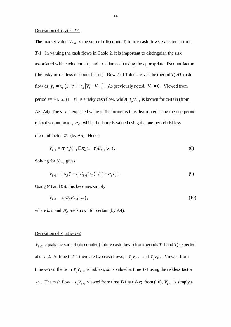
Derivation of Vs at s=T-1

The market value 1TV − is the sum of (discounted) future cash flows expected at time

T-1. In valuing the cash flows in Table 2, it is important to distinguish the risk

associated with each element, and to value each using the appropriate discount factor

(the risky or riskless discount factor). Row T of Table 2 gives the (period T) AT cash

flow as ( ) [ ]11T T g T Tx V Vχ τ τ −= − − − . As previously noted, 0TV = . Viewed from

period s=T-1, ( )1Tx τ− is a risky cash flow, whilst 1g TVτ − is known for certain (from

A3, A4). The s=T-1 expected value of the former is thus discounted using the one-period

risky discount factor, βπ , whilst the latter is valued using the one-period riskless

discount factor fπ (by A5). Hence,

1 1 1(1 ) ( )T f g T T TV V E xβπ τ π τ− − −= + − . (8)

Solving for 1TV − gives

1 1(1 ) ( ) 1T T T f gV E xβπ τ π τ− −

� ��� �= − −� ��� � . (9)

Using (4) and (5), this becomes simply

1 1( )T T TV ka E xβπ− −= , (10)

where k, a and βπ are known for certain (by A4).

Derivation of Vs at s=T-2

2TV − equals the sum of (discounted) future cash flows (from periods T-1 and T) expected

at s=T-2. At time t=T-1 there are two cash flows; - 1g TVτ − and 2g TVτ − . Viewed from

time s=T-2, the term 2g TVτ − is riskless, so is valued at time T-1 using the riskless factor

fπ . The cash flow 1g TVτ −− viewed from time T-1 is risky; from (10), 1TV − is simply a

15

constant multiplied by 1( )T TE x− , so, by assumptions A3 and A5, the appropriate one-

period discount factor for valuing this term is βπ .

There are also two non-zero cash flows arising at time T, namely 1g TVτ − and ( )1 Txτ− .

To obtain the present values for these, their s=T-2 expected values must be discounted

two periods. The first cash flow, 1g TVτ − , is a random variable which from (10) is a scalar

multiple of 1( )T TE x− up until time T-1, and thereafter is known for certain. Hence the

two-period discount factor for 2 1( )g T TE Vτ − − is fβπ π . The second cash flow, ( )1 Txτ− ,

is a random variable, with risk β in each period (assumption A3). The two-period

discount factor for ( ) 21 ( )T TE xτ −− is therefore 2βπ .

Adding the values for t=T–1 and t=T cash flows,

22 2 2 1 2 1 2( ) ( ) (1 ) ( )T f g T g T T f g T T T TV V E V E V E xβ β βπ τ π τ π π τ π τ− − − − − − −= − + + − , (11)

so, solving for 2TV − gives

22 2 1 2( 1) ( ) (1 ) ( ) 1T f g T T T T f gV E V E xβ βπ π τ π τ π τ− − − −

� � � �= − + − −� �� � . (12)

To simplify equation (12) further, note that, by the law of iterated expectations (see e.g.

Hamilton [1994 p. 742]), for any arbitrarily chosen cash flow, Tx ,

( )( ) ( )s t T s TE E x E x= for all , ,s t T such that 0 s t T≤ ≤ ≤ . Now, using (9),

( )2 1 2 1

2

( ) (1 ) ( ) 1

(1 ) ( ) 1

T T T T T f g

T T f g

E V E E x

E x

β

β

π τ π τ

π τ π τ

− − − −

−

� ��� �= − −� ��� �

� �� �= − −� �� �

. (13)

Substituting into (12) then gives

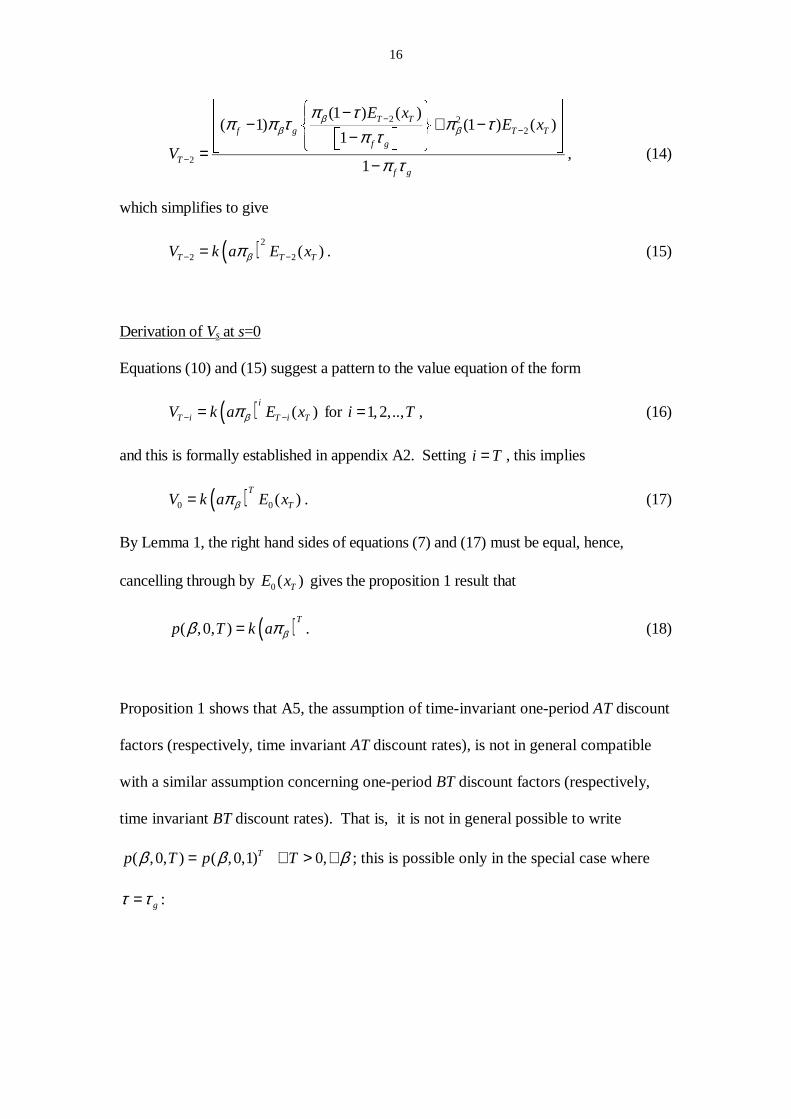
16

2 22

2

(1 ) ( )( 1) (1 ) ( )

1

1

T Tf g T T

f g

Tf g

E xE x

V

ββ β

π τπ π τ π τ

π τ

π τ

−−

−

� �� �−

� �� �

− + −� �

� �−

� �� � � �

=−

, (14)

which simplifies to give

( )2

2 2( )T T TV k a E xβπ− −= . (15)

Derivation of Vs at s=0

Equations (10) and (15) suggest a pattern to the value equation of the form

( ) ( )i

T i T i TV k a E xβπ− −= for 1,2,..,i T= , (16)

and this is formally established in appendix A2. Setting i T= , this implies

( )0 0( )T

TV k a E xβπ= . (17)

By Lemma 1, the right hand sides of equations (7) and (17) must be equal, hence,

cancelling through by 0( )TE x gives the proposition 1 result that

( )( ,0, )T

p T k a ββ π= . (18)

Proposition 1 shows that A5, the assumption of time-invariant one-period AT discount

factors (respectively, time invariant AT discount rates), is not in general compatible

with a similar assumption concerning one-period BT discount factors (respectively,

time invariant BT discount rates). That is, it is not in general possible to write

( ,0, ) ( ,0,1)Tp T pβ β= 0,T β∀ > ∀ ; this is possible only in the special case where

gτ τ= :

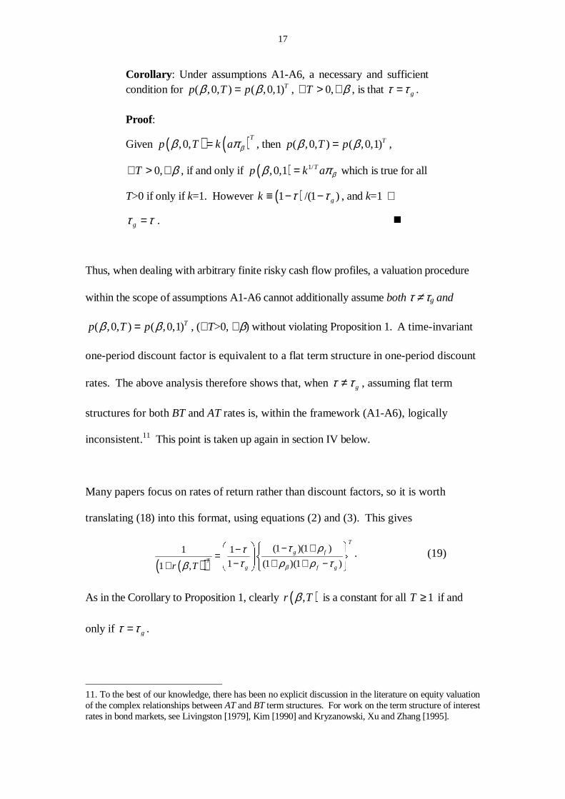
17

Corollary: Under assumptions A1-A6, a necessary and sufficient condition for ( ,0, ) ( ,0,1)Tp T pβ β= , 0,T β∀ > ∀ , is that gτ τ= .

Proof:

Given ( ) ( ),0,T

p T k a ββ π= , then ( ,0, ) ( ,0,1)Tp T pβ β= ,

0,T β∀ > ∀ , if and only if ( ) 1/,0,1 Tp k a ββ π= which is true for all

T>0 if only if k=1. However ( )1 /(1 )gk τ τ≡ − − , and k=1 ⇔

gτ τ= . �

Thus, when dealing with arbitrary finite risky cash flow profiles, a valuation procedure

within the scope of assumptions A1-A6 cannot additionally assume both τ ≠ τg and

( ,0, ) ( ,0,1)Tp T pβ β= , (∀T>0, ∀β) without violating Proposition 1. A time-invariant

one-period discount factor is equivalent to a flat term structure in one-period discount

rates. The above analysis therefore shows that, when gτ τ≠ , assuming flat term

structures for both BT and AT rates is, within the framework (A1-A6), logically

inconsistent.11 This point is taken up again in section IV below.

Many papers focus on rates of return rather than discount factors, so it is worth

translating (18) into this format, using equations (2) and (3). This gives

( )( )

(1 )(1 )1 1

1 (1 )(1 )1 ,

T

g f

Tg f gr T β

τ ρττ ρ ρ τβ

����� �− +− � �= � � ��− + + −+ � � ���� � . (19)

As in the Corollary to Proposition 1, clearly ( ),r Tβ is a constant for all 1T ≥ if and

only if gτ τ= .

11. To the best of our knowledge, there has been no explicit discussion in the literature on equity valuation of the complex relationships between AT and BT term structures. For work on the term structure of interest rates in bond markets, see Livingston [1979], Kim [1990] and Kryzanowski, Xu and Zhang [1995].

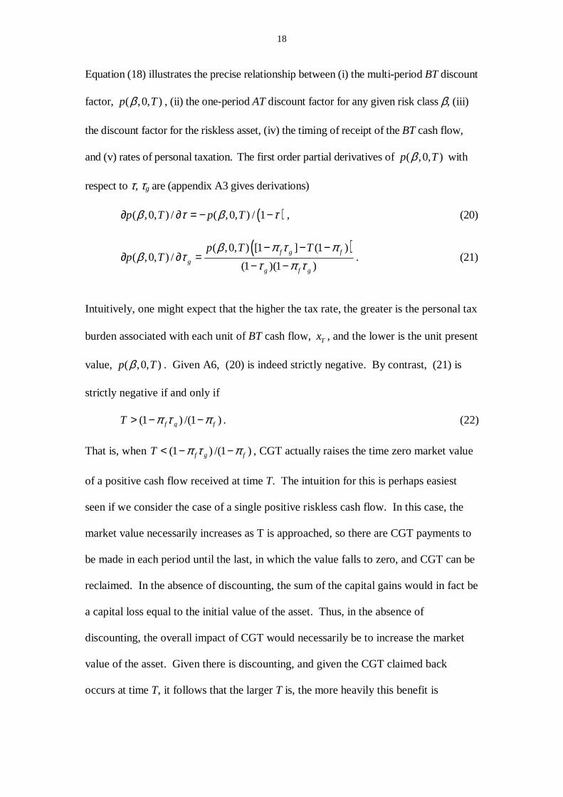
18

Equation (18) illustrates the precise relationship between (i) the multi-period BT discount

factor, ( ,0, )p Tβ , (ii) the one-period AT discount factor for any given risk class β, (iii)

the discount factor for the riskless asset, (iv) the timing of receipt of the BT cash flow,

and (v) rates of personal taxation. The first order partial derivatives of ( ,0, )p Tβ with

respect to τ, τg are (appendix A3 gives derivations)

( )( ,0, ) / ( ,0, ) / 1p T p Tβ τ β τ∂ ∂ = − − , (20)

( )( ,0, ) [1 ] (1 )

( ,0, ) /(1 )(1 )

f g f

gg f g

p T Tp T

β π τ πβ τ

τ π τ− − −

∂ ∂ =− −

. (21)

Intuitively, one might expect that the higher the tax rate, the greater is the personal tax

burden associated with each unit of BT cash flow, Tx , and the lower is the unit present

value, ( ,0, )p Tβ . Given A6, (20) is indeed strictly negative. By contrast, (21) is

strictly negative if and only if

(1 ) /(1 )f g fT π τ π> − − . (22)

That is, when (1 ) /(1 )f g fT π τ π< − − , CGT actually raises the time zero market value

of a positive cash flow received at time T. The intuition for this is perhaps easiest

seen if we consider the case of a single positive riskless cash flow. In this case, the

market value necessarily increases as T is approached, so there are CGT payments to

be made in each period until the last, in which the value falls to zero, and CGT can be

reclaimed. In the absence of discounting, the sum of the capital gains would in fact be

a capital loss equal to the initial value of the asset. Thus, in the absence of

discounting, the overall impact of CGT would necessarily be to increase the market

value of the asset. Given there is discounting, and given the CGT claimed back

occurs at time T, it follows that the larger T is, the more heavily this benefit is

19

discounted, and so the more likely it becomes that the impact of CGT is no longer

beneficial.12 13

Having spent some time discussing the role of CGT, it is worth emphasising that the

non-linearity in the transformation from AT to BT discount factors does not disappear

when CGT is zero. This point has already been made in our numerical example in

section 1. More formally, it can be seen by setting gτ =0 in (19). This then simplifies

to give

( )( )

( ) ( ) ( ) 1/111 , (1 ) 1

(1 )1 ,

T

T T r Tr T

ββ

τβ ρ τ

ρβ−−

= � + = + −++

(23)

That is, if 0τ > whilst 0gτ = , ( ),r Tβ continues to be a non-linear function of T, and

so, even if 0gτ = , it is not possible to assume that both BT and AT term structures are

flat.

III. Level perpetuities and the Miller [1977] model The (risky) level perpetuity is an important special case where a simpler relationship

between BT and AT discount factors exists. This perpetuity offers risky BT cash

payments, Tx for T=1,...,∞. It is characterised by the condition ( )0 TE x x= , a

constant, for all T>0. The level perpetuity is assumed to have a constant level of

12. More formally, inspection of Table 2 indicates that the capital gains tax saving at time T, (τg(VT-1-VT) = τgVT-1), is greater in absolute magnitude than the total of capital gains tax payments from t=1 through T-1, (Σtτg(Vt-Vt-1) = τg(VT-1-V0)). But when receipt of this tax saving is sufficiently distant (large T) and/or the time discounts are sufficiently large, the total present value of the stream of expected capital gains tax cash flows will be negative. Then, since the payment of capital gains tax reduces present value, the higher is τg, the lower is p(β,0,T).

13 Focusing on a single cash flow thus seems to suggest that investors would want to lobby to increase the CGT rate in this framework. However that is not the case, because many of the assets that concern investors are perpetual and growing assets for which CGT is indeed a burden. This is explained in detail in section 4 below.

20

‘ riskiness’ (or ‘homogenous’ risk) in the sense that the time-invariant per-period risk

of each expected cash flow is a constant β across all expected cash flows making up

the perpetuity. However, note that a risky level perpetuity is level only in the sense that

time zero expectations of the risky future cash flows are constants. Its value will actually

fluctuate randomly as time passes. The procedure for valuing the risky level perpetuity

is exactly the same as for any arbitrary set of cash flows; each cash flow is valued

separately, and then the values are summed. It is worth emphasising that every cash

flow in the risky perpetuity gives rise to a stream of capital gains/losses as per Table 2 –

so it follows, a fortiori, that there is a stream of capital gains tax cash flows associated

with such a perpetuity.14

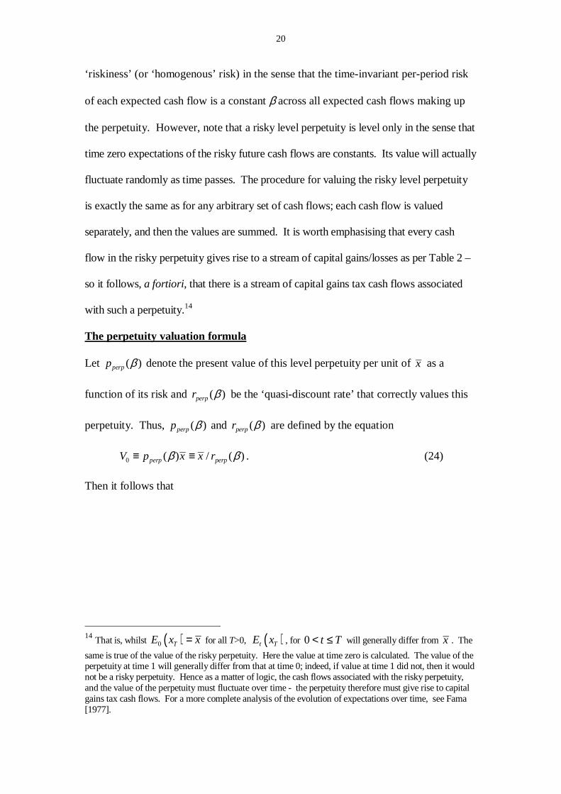
The perpetuity valuation formula

Let ( )perpp β denote the present value of this level perpetuity per unit of x as a

function of its risk and ( )perpr β be the ‘quasi-discount rate’ that correctly values this

perpetuity. Thus, ( )perpp β and ( )perpr β are defined by the equation

0 ( ) / ( )perp perpV p x x rβ β≡ ≡ . (24)

Then it follows that

14 That is, whilst ( )0 TE x x= for all T>0, ( )t TE x , for 0 t T< ≤ will generally differ from x . The

same is true of the value of the risky perpetuity. Here the value at time zero is calculated. The value of the perpetuity at time 1 will generally differ from that at time 0; indeed, if value at time 1 did not, then it would not be a risky perpetuity. Hence as a matter of logic, the cash flows associated with the risky perpetuity, and the value of the perpetuity must fluctuate over time - the perpetuity therefore must give rise to capital gains tax cash flows. For a more complete analysis of the evolution of expectations over time, see Fama [1977].

21

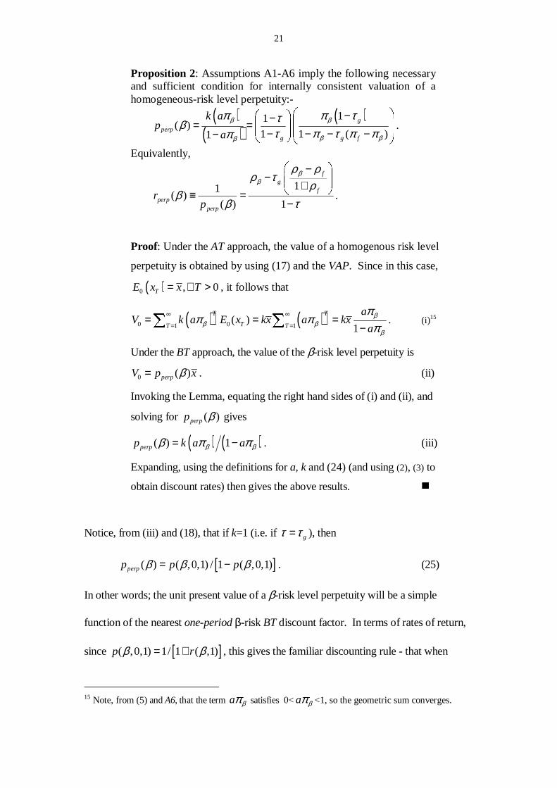
Proposition 2: Assumptions A1-A6 imply the following necessary and sufficient condition for internally consistent valuation of a homogeneous-risk level perpetuity:-

( )

( )( )11

( )1 1 ( )1

g

perpg g f

k ap

a

β β

β ββ

π π ττβτ π τ π ππ

� �−

���− � �= = � �� � � �− − − −− ��� � �

.

Equivalently,

11

( )( ) 1

fg

f

perpperp

rp

ββ

ρ ρρ τ

ρβ

β τ

� �−

− +� �≡ =

−.

Proof: Under the AT approach, the value of a homogenous risk level

perpetuity is obtained by using (17) and the VAP. Since in this case,

( )0 , 0TE x x T= ∀ > , it follows that

( ) ( )0 01 1( )

1

T T

TT T

aV k a E x kx a kx

aβ

β ββ

ππ π

π∞ ∞

= == = =

−

. (i)15

Under the BT approach, the value of the β-risk level perpetuity is

0 ( )perpV p xβ= . (ii)

Invoking the Lemma, equating the right hand sides of (i) and (ii), and

solving for ( )perpp β gives

( ) ( )( ) 1perpp k a aβ ββ π π= − . (iii)

Expanding, using the definitions for a, k and (24) (and using (2), (3) to

obtain discount rates) then gives the above results. �

Notice, from (iii) and (18), that if k=1 (i.e. if gτ τ= ), then

[ ]( ) ( ,0,1) / 1 ( ,0,1)perpp p pβ β β= − . (25)

In other words; the unit present value of a β-risk level perpetuity will be a simple

function of the nearest one-period β-risk BT discount factor. In terms of rates of return,

since [ ]( ,0,1) 1/ 1 ( ,1)p rβ β= + , this gives the familiar discounting rule - that when

15 Note, from (5) and A6, that the term a βπ satisfies 0< a βπ <1, so the geometric sum converges.

22

gτ τ= , the value of the risky level perpetuity is simply the BT expected cash flow

divided by the BT one period discount rate; that is, the BT valuation rule is simply

0 ( ,1)V x r β= . (26)

However, it must be stressed that this holds only if k=1; that is, only if gτ τ= .

Notice also, from Proposition 2, for a riskless perpetuity, since fβ = , it follows that

( )( ) 1perp fr f ρ τ= − . (27)

That is, the ‘quasi-discount rate’ to correctly value a BT riskless level perpetuity is

simply the ‘grossed up’ AT discount rate. Also, for a risky level perpetuity, if the capital

gains tax rate is zero, then, from Proposition 2,

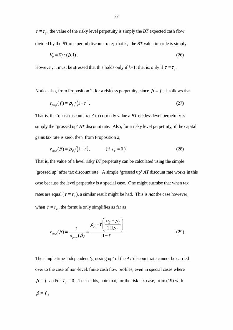
( )( ) 1perpr ββ ρ τ= − , (if 0gτ = ). (28)

That is, the value of a level risky BT perpetuity can be calculated using the simple

‘grossed up’ after tax discount rate. A simple ‘grossed up’ AT discount rate works in this

case because the level perpetuity is a special case. One might surmise that when tax

rates are equal ( gτ τ= ), a similar result might be had. This is not the case however;

when gτ τ= , the formula only simplifies as far as

11

( )( ) 1

f

f

perpperp

rp

ββ

ρ ρρ τ

ρβ

β τ

� �−

− � �� �+� �≡ =

−. (29)

The simple time-independent ‘grossing up’ of the AT discount rate cannot be carried

over to the case of non-level, finite cash flow profiles, even in special cases where

fβ = and/or 0gτ = . To see this, note that, for the riskless case, from (19) with

fβ = ,

23

( )( )

11 1

1 11 ,

T

g

Tg f gr f T

τττ ρ τ

����� �−−= � � � �� � � �− + −+ ����� �

, (30)

whilst the case with 0gτ = , from (19), gives

( )( )

( )1 11

11 ,

T

Tr T β

τρβ

� = − � �++ �

. (31)

With both fβ = and 0gτ = , (19) gives

( )( )

( )1 11

11 ,

T

Tfr f T

τρ

� �= − � �� �++ � �

. (32)

Thus in all these cases, the transformation from AT to BT is a non-linear function of the

time to receipt of the cash flow.

Why CGT can ‘add value’

In the special case of the level perpetuity, Proposition 2 shows that there is a strictly

positive relationship between the capital gains tax rate and market value when the

perpetuity is risky, fβρ ρ> : that is, from (29),

( )1

( ) 0

1

perpperp

gfg

f

pp

ββ

βτβτρ ρ

ρ τρ

∂−= � >∂

� �−

− � �� �+� � (33)

Readers of an earlier version of the paper found this result rather puzzling (and ‘counter-

intuitive’). For this reason it is worth examining it in more detail. A useful way to do so

is to examine the case where the perpetuity features a constant expected growth rate g

(which could be zero as a special case). Consider the result of buying such a risky

perpetuity and selling it after one period. The cash flows that arise are as follows:

24

Table 3 Cash flows for a one period buy and sell strategy

Time period: Cash flow 0

0V− (initial payment)

1 1V� (sale at market value, a random variable)

1 1 0( ) gV V τ− −

� (CGT payment)

1 1(1 )x τ−

� (receipt of tx

� and payment of tax on it)

The claim against initial value in the CGT payment, 0 gV τ , is riskless and so must be

discounted at the riskless rate; all the other elements of the return are risky and so are

discounted at βρ . Hence, defining 1 0 1( )x E x≡�

and 1 0 1( )V E V≡�

, then in equilibrium

1 1 1 00

(1 )

1 1g g

f

V x V VV

β

τ τ τρ ρ

+ − −= +

+ + (34)

The expected cash flows, and hence expected values, grow at the rate g (as in Gordon’s

dividend growth valuation model), so

10 1( ) (1 )t

t tx E x g x−≡ = +�

( �0 0( ) (1 )t

t tV E V g V≡ = +�

) (35)

Using this to substitute for 1V in (34) (and rearranging) gives the valuation formula

10

(1 )

1f

gf

xV

g gββ

τρ ρ

ρ τρ

−= −

− − −� �� �

+ �

. (36)

As before (Proposition 2), when g=0, increases in CGT add value. The intuition for this

can be seen by inspection of the cash flows at time period 1 in Table 3. From (35),

notice that 0 1 0 1 0 0( )E V V V V gV− = − =�

; thus if g=0, the expected value at time 0 of CGT

payments at time 1 is zero. However, if g=0, the present value of this CGT tax payment

is negative; this arises because the allowance against the opening balance 0V is riskless

and so is discounted less heavily than the risky CGT payment on 1V� . To spell this out,

25

0 1 0 0 0( ) (1 )( )

1 1 1 1g g g g

f f

E V V g V VPV CGT

β β

τ τ τ τρ ρ ρ ρ

+= − = −

+ + + +

�

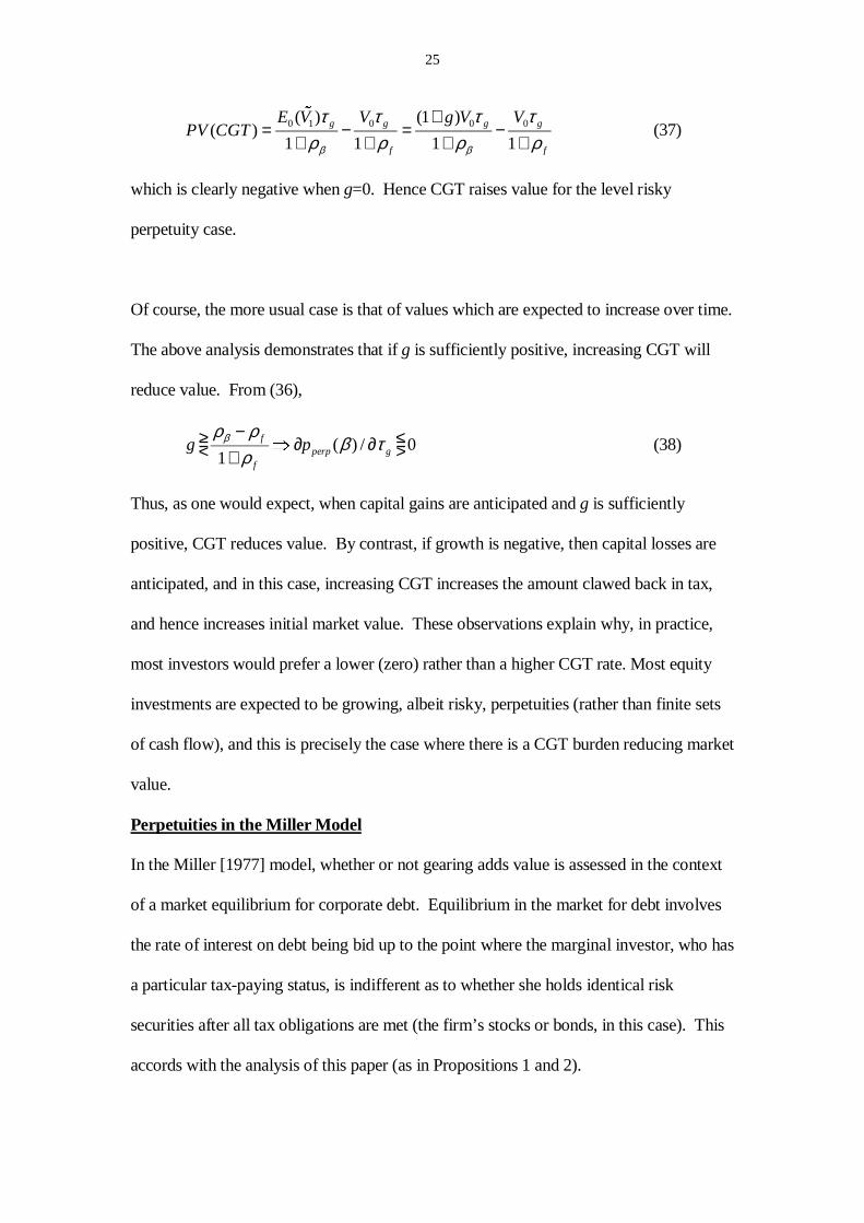
(37)

which is clearly negative when g=0. Hence CGT raises value for the level risky

perpetuity case.

Of course, the more usual case is that of values which are expected to increase over time.

The above analysis demonstrates that if g is sufficiently positive, increasing CGT will

reduce value. From (36),

( ) / 01

fperp g

f

g pβρ ρβ τ

ρ−> <= � ∂ ∂ =< >+

(38)

Thus, as one would expect, when capital gains are anticipated and g is sufficiently

positive, CGT reduces value. By contrast, if growth is negative, then capital losses are

anticipated, and in this case, increasing CGT increases the amount clawed back in tax,

and hence increases initial market value. These observations explain why, in practice,

most investors would prefer a lower (zero) rather than a higher CGT rate. Most equity

investments are expected to be growing, albeit risky, perpetuities (rather than finite sets

of cash flow), and this is precisely the case where there is a CGT burden reducing market

value.

Perpetuities in the Miller Model

In the Miller [1977] model, whether or not gearing adds value is assessed in the context

of a market equilibrium for corporate debt. Equilibrium in the market for debt involves

the rate of interest on debt being bid up to the point where the marginal investor, who has

a particular tax-paying status, is indifferent as to whether she holds identical risk

securities after all tax obligations are met (the firm’s stocks or bonds, in this case). This

accords with the analysis of this paper (as in Propositions 1 and 2).

26

The Miller [1977] debt and taxes paper deals with a special case for simplicity -

specifically, it features riskless and permanent debt along with a risky operating cash

flow perpetuity. There are no taxes on equity, and a single time invariant investor

specific tax rate is used for ‘ income from bonds’ (Miller [1977, p. 267]: denoted PBατ in

that paper). The rate 0r in that paper denoted the ‘equilibrium rate of interest on fully

tax exempt bonds’ (p. 268). It is therefore not only the BT discount rate for the latter, but

also the AT discount rate for all investors and for all riskless securities. In equilibrium,

the BT price of a taxable riskless bond must have adjusted to the point where the AT

riskless return for the marginal investor (the “ α -investor” paying tax at the rate PBατ )

equals 0r . That is, in equilibrium,

( ) 0( ) 1d PBr B rατ− = , (39)

where ( )dr B denotes the inverse demand function for debt. Thus, (39) implies the rate

of interest on debt is bid up to the point where, in equilibrium,

0( )1d

PB

rr B ατ

=−

. (40)

This formulation corresponds to the result established in Proposition 2 above for a level

riskless perpetuity. It does not, of course, hold for arbitrary finite cash flow profiles,

where the BT rates which ensure AT equilibrium are more complex (as indicated in

Proposition 1).

Miller [1977] does also briefly consider the risky perpetuity case, but says little about

how the relationship between BT and AT rates is changed for this case, commenting

“Default risk can be accommodated… by merely reinterpreting all the before-tax

interest rates as risk adjusted or certainty equivalent rates.” (p. 271). This appears to

27

suggest that the simple ‘grossing-up’ procedure above remains valid for moving from AT

to BT interest rates when dealing with risky bonds. However, the above analysis shows

that this is not correct - except, of course, for the special case of the level risky perpetuity

when the rate of taxation on capital gains is zero (as in equation (28)).

Recall that in the Miller [1977] model, PBατ is used as the rate of taxation for ‘ income

from bonds’. Income includes cash disbursements and capital gains. For the level

riskless perpetuity, there are no capital gains, hence income is equal to cash

disbursements. However, for most other cases, including that of risky level perpetuities,

income is not equal to cash disbursements. Given the debt marginal rate PBατ in Miller

[1977] applies to income, it would appear that, implicitly, debt capital gains and cash

disbursements (the two components of income) are taxed at the same rate, ruling out a

zero capital gains tax rate for debt. If so, the simple ‘grossing up’ formula of type (40)

cannot be applied in such a case. Logically therefore, whilst the general thrust of the

Miller model obviously makes sense, the formal ‘model’ as sketched in the 1977 paper

works in the way described there only if it is restricted to the case where debt is

perpetual, constant and riskless, the equity cash flow is a level risky perpetuity, and the

tax rate on equity capital gains is zero.

IV. BT and AT discount rates in the literature This section examines the surveyed works which focus on the valuation of non-level and

finite risky cash flow profiles in the presence of personal taxes (Clubb & Doran [1991,

1992], Appleyard & Strong [1989], Strong & Appleyard [1992] and Taggart [1991]).

There are, within the framework of assumptions A1-A6, generally five determinants of

multi-period BT discount factors, and four in the special case of a level perpetuity. Two

28

determinants are asset-specific: risk, reflected in βπ , and the number of periods, T

(which is not relevant, of course, in the case of the perpetuity). The remainder are

general parameters: tax rates, τ and τg, and the riskless one-period AT discount factor

fπ . This latter determinant arises from the tax deductibility of capital investments in

calculating capital gains tax liability; such investments are always known for certain one

period before discharge of the liability.

Turning now to the above literature, first note that all five surveyed models employ time-

invariant one-period BT discount factors. In accordance with the Corollary to Proposition

1, within the specified framework (assumptions A1-A6), time-invariant one-period BT

discount factors are incompatible with the assumption of time-invariant AT discount

factors unless the rates of taxation, τ and τg, are equal. By the corollary to proposition 1,

for these models to be internally consistent, the condition τ = τg (i.e. k=1) must therefore

hold as an explicit or implicit assumption. However, the model proposed in Clubb &

Doran [1991], in explicitly assuming a zero level of equity capital gains tax (thus setting

0gτ τ> = for these equity tax rates), violates the Corollary (which establishes that,

when gτ τ> , it is inadmissible to assume that both BT and AT term structures for

discount rates are flat.16

Of the remaining four models, Clubb and Doran [1992] explicitly assume gτ τ= , whilst

the other papers assume a constant overall or effective rate of tax on equity cash flows.

16 The relationship between AT and BT discount rates established in proposition 1 is intrinsically non-linear

when gτ τ> . The nonlinearity in the translation between AT and BT rates needs to be recognized even in

the more general case where the AT term structure has an arbitrary shape.

29

We have already established that this is formally equivalent to making assumption A2

for CGT and also to assuming that gτ τ= (proof in appendix 1). These models also

assume a relationship between BT and AT discount rates of the form

( ,1)1

r βρβ

τ=

−, (41)

which, using equations (2) and (3), gives a discount factor of the form

(1 )

( ,0,1)1

p β

β

π τβ

π τ−

=−

. (42)

With gτ τ= , from (4), k=1. However, equation (18) shows that, for k=1,

( )

( )1

( ,0,1)1 f

p a ββ

π τβ π

π τ−

= =−

. (43)

In a world of personal taxes (τ>0), the right hand sides of equations (42) and (43) will

be equal (and will therefore satisfy Propositions 1 and 2) if and only if β=f. That is, if

and only if all the cash flows are riskless. Since the models in Appleyard & Strong

[1989] and Strong & Appleyard [1992] both assume the relationship in (42) holds for all

types of cash flow whether risky or not (i.e. β≠f), these models are internally

inconsistent, failing to properly account for the effect of the non-zero capital gains tax.

The remaining two models, Clubb & Doran [1992] and Taggart [1991], employ the

relationship in (42) only in the case of riskless cash flows. By restricting attention to this

(rather limiting) special case, these models are internally coherent, at least by the test

applied in the present paper.

V. Sensitivity Analysis Whilst the primary object was to examine the theoretical relationship between BT and

AT discount rates and factors and to examine whether these had been consistently used in

the literature, it is of some interest to explore numerically the non-linear relationship

30

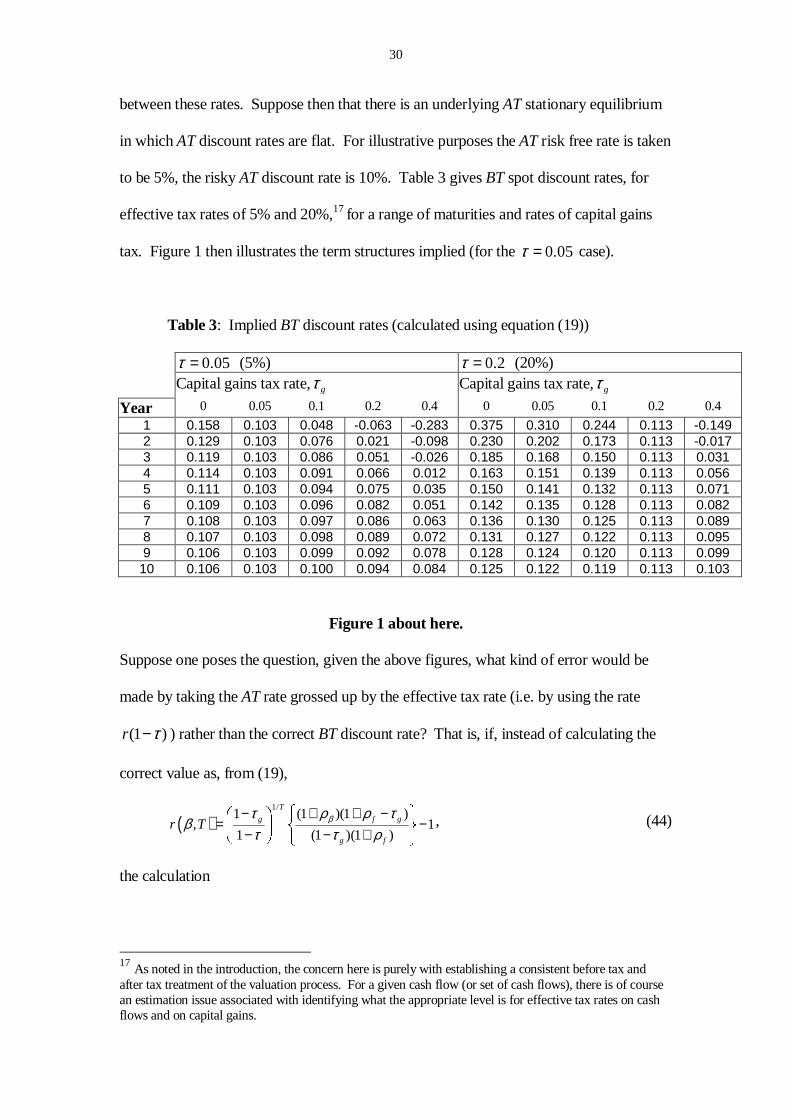
between these rates. Suppose then that there is an underlying AT stationary equilibrium

in which AT discount rates are flat. For illustrative purposes the AT risk free rate is taken

to be 5%, the risky AT discount rate is 10%. Table 3 gives BT spot discount rates, for

effective tax rates of 5% and 20%,17 for a range of maturities and rates of capital gains

tax. Figure 1 then illustrates the term structures implied (for the 0.05τ = case).

Table 3: Implied BT discount rates (calculated using equation (19))

0.05τ = (5%) 0.2τ = (20%) Capital gains tax rate, gτ Capital gains tax rate, gτ

Year 0 0.05 0.1 0.2 0.4 0 0.05 0.1 0.2 0.4

1 0.158 0.103 0.048 -0.063 -0.283 0.375 0.310 0.244 0.113 -0.149 2 0.129 0.103 0.076 0.021 -0.098 0.230 0.202 0.173 0.113 -0.017 3 0.119 0.103 0.086 0.051 -0.026 0.185 0.168 0.150 0.113 0.031 4 0.114 0.103 0.091 0.066 0.012 0.163 0.151 0.139 0.113 0.056 5 0.111 0.103 0.094 0.075 0.035 0.150 0.141 0.132 0.113 0.071 6 0.109 0.103 0.096 0.082 0.051 0.142 0.135 0.128 0.113 0.082 7 0.108 0.103 0.097 0.086 0.063 0.136 0.130 0.125 0.113 0.089 8 0.107 0.103 0.098 0.089 0.072 0.131 0.127 0.122 0.113 0.095 9 0.106 0.103 0.099 0.092 0.078 0.128 0.124 0.120 0.113 0.099

10 0.106 0.103 0.100 0.094 0.084 0.125 0.122 0.119 0.113 0.103

Figure 1 about here.

Suppose one poses the question, given the above figures, what kind of error would be

made by taking the AT rate grossed up by the effective tax rate (i.e. by using the rate

(1 )r τ− ) rather than the correct BT discount rate? That is, if, instead of calculating the

correct value as, from (19),

( )1/

1 (1 )(1 ), 1

1 (1 )(1 )

T

g f g

g f

r T βτ ρ ρ τβ

τ τ ρ

� �− + + −��� � �

= −� ��

− − +� ���� � , (44)

the calculation

17 As noted in the introduction, the concern here is purely with establishing a consistent before tax and after tax treatment of the valuation process. For a given cash flow (or set of cash flows), there is of course an estimation issue associated with identifying what the appropriate level is for effective tax rates on cash flows and on capital gains.

31

( )ˆ ,(1 )

r T βρβ

τ=

− (45)

is used. Retaining the same parameter values ( 0.05fρ = , 0.1βρ = , 0.05τ = or 0.2) it is

then possible to calculate the percentage error in the calculation of the BT discount rate

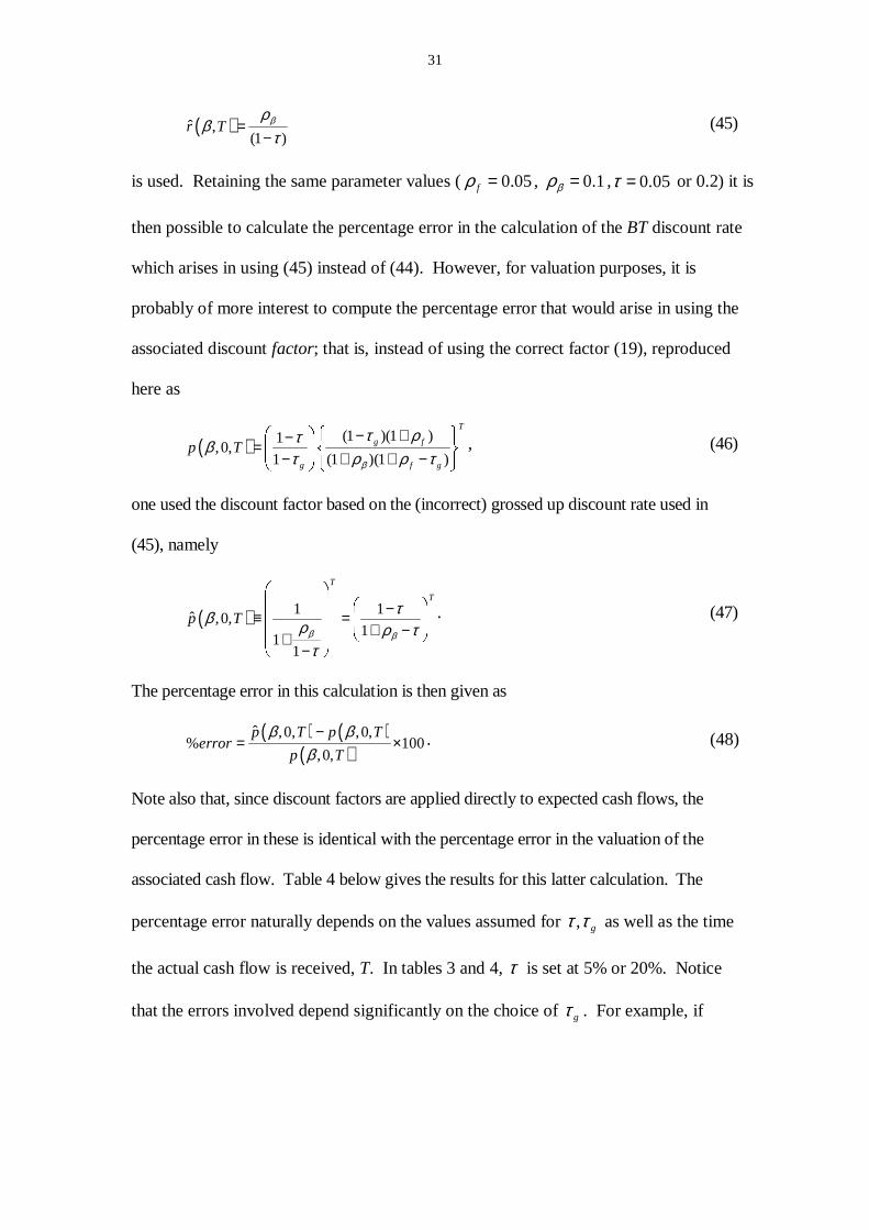
which arises in using (45) instead of (44). However, for valuation purposes, it is

probably of more interest to compute the percentage error that would arise in using the

associated discount factor; that is, instead of using the correct factor (19), reproduced

here as

( ) (1 )(1 )1,0,

1 (1 )(1 )

T

g f

g f g

p Tβ

τ ρτβτ ρ ρ τ

����� �− +− � �= �� ���− + + −� ��� �� � , (46)

one used the discount factor based on the (incorrect) grossed up discount rate used in

(45), namely

( ) 1 1ˆ ,0,

11

1

T

T

p Tβ β

τβ ρ ρ ττ

� �� � � �−≡ =

� � � �� �+ −

� � � �+� �

−� �

. (47)

The percentage error in this calculation is then given as

( ) ( )( )

ˆ ,0, ,0,% 100

,0,

p T p Terror

p T

β ββ

−= × . (48)

Note also that, since discount factors are applied directly to expected cash flows, the

percentage error in these is identical with the percentage error in the valuation of the

associated cash flow. Table 4 below gives the results for this latter calculation. The

percentage error naturally depends on the values assumed for , gτ τ as well as the time

the actual cash flow is received, T. In tables 3 and 4, τ is set at 5% or 20%. Notice

that the errors involved depend significantly on the choice of gτ . For example, if

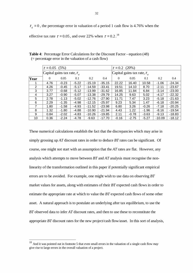
32

0gτ = , the percentage error in valuation of a period 1 cash flow is 4.76% when the

effective tax rate 0.05τ = , and over 22% when 0.2τ = .18

Table 4: Percentage Error Calculations for the Discount Factor - equation (48) (= percentage error in the valuation of a cash flow) 0.05τ = (5%) 0.2τ = (20%) Capital gains tax rate, gτ Capital gains tax rate, gτ

Year 0 0.05 0.1 0.2 0.4 0 0.05 0.1 0.2 0.4

1 4.76 -0.23 -5.22 -15.19 -35.15 22.22 16.40 10.58 -1.06 -24.34 2 4.26 -0.45 -5.17 -14.59 -33.41 19.51 14.10 8.70 -2.11 -23.67 3 3.77 -0.68 -5.12 -13.99 -31.62 16.85 11.84 6.84 -3.14 -23.00 4 3.27 -0.90 -5.07 -13.38 -29.79 14.25 9.63 5.02 -4.17 -22.32 5 2.78 -1.13 -5.02 -12.76 -27.90 11.71 7.47 3.23 -5.18 -21.63 6 2.29 -1.35 -4.98 -12.15 -25.97 9.23 5.34 1.47 -6.18 -20.94 7 1.80 -1.58 -4.93 -11.52 -23.98 6.80 3.26 -0.26 -7.18 -20.25 8 1.32 -1.80 -4.88 -10.90 -21.94 4.43 1.22 -1.96 -8.16 -19.54 9 0.84 -2.02 -4.83 -10.26 -19.85 2.11 -0.78 -3.63 -9.13 -18.83

10 0.36 -2.24 -4.78 -9.63 -17.70 -0.16 -2.75 -5.27 -10.09 -18.12

These numerical calculations establish the fact that the discrepancies which may arise in

simply grossing up AT discount rates in order to deduce BT rates can be significant. Of

course, one might not start with an assumption that the AT rates are flat. However, any

analysis which attempts to move between BT and AT analysis must recognise the non-

linearity of the transformation outlined in this paper if potentially significant empirical

errors are to be avoided. For example, one might wish to use data on observing BT

market values for assets, along with estimates of their BT expected cash flows in order to

estimate the appropriate rate at which to value the BT expected cash flows of some other

asset. A natural approach is to postulate an underlying after tax equilibrium, to use the

BT observed data to infer AT discount rates, and then to use these to reconstitute the

appropriate BT discount rates for the new project/cash flow/asset. In this sort of analysis,

18 And it was pointed out in footnote 5 that even small errors in the valuation of a single cash flow may give rise to large errors in the overall valuation of a project.

33

as has been established in this paper, the move from BT to AT and back again must be

done with some care.

VI. Summary The literature extending the Miles-Ezzell ADMP approach to the case of valuing

arbitrary finite risky cash flow profiles in the presence of personal taxes is aimed at

furnishing a realistic yet practical approach to the capital budgeting problem. A

general starting point, explicit or implicit in this literature, is that the simple linear

relationship between BT and AT discount rates and the effective tax rate found in

Miller [1977] carries through to more general settings than the case where debt is

riskless and fixed in perpetuity and where equity income evades all personal taxes. It

is shown in this paper that Miller’s specific model is an unproblematic special case

precisely because it does assume the cash flow is a riskless perpetuity and that the

capital gains tax rate is zero. Any extensions of the ‘debt and taxes’ model to

incorporate positive equity tax rates – or risky debt – would seem to require a more

careful treatment of the BT/AT relationship identified in this paper.

The relationships identified here between AT and BT discount factors (discount rates)

have received no attention in the literature on valuation of equities in the presence of

personal taxes (although related issues have been discussed in work on the valuation of

bonds). Even those articles which do not suffer from the inconsistency problem

identified here do not discuss, or even mention, this issue. This suggests that the

relationships discussed in this paper may not be widely known or understood (as

manifest by the fact that several papers in the above literature develop models based on

assumptions which turn out to be internally incoherent). Specifically, the models of

34

Clubb & Doran [1991], Appleyard & Strong [1989] and Strong & Appleyard [1991] are

found to be based upon internally contradictory assumptions; the valuation formulae

derived in these papers are consequently unreliable. The models contained in Miller

[1977], Clubb & Doran [1992] and Taggart [1991] are confined to special cases where it

turns out the model assumptions are internally consistent (although there is no discussion

in these papers of why there is a need to confine attention to these rather special cases).

At an empirical level, the magnitude of the potential error that might be incurred by

assuming that both rates of taxation and BT/AT term structures are flat has been shown to

be potentially quite significant.19 The present paper clarifies the issues involved, such

that any future modelling in this area will not suffer from internal inconsistencies of the

type described above.

REFERENCES

Appleyard, T. R. & N. C. Strong, 1989, Beta Geared and Ungeared: The Case of Active

Debt Management, Accounting and Business Research, Vol. 19, pp. 170-174. Auerback A. J., 1991, Retrospective capital gains taxation, American Economic

Review, 81, 167-178. Brealey R.A. and Myers S.C., 1996, Principles of Corporate Finance, 5 Ed., McGraw

Hill, New York. Buckley A., Ross S.A., Westerfield R.W. and Jaffe J., 1998, Corporate Finance

Europe, McGraw Hill, London. Clubb, C. D. B & P. Doran, 1991, Beta Geared and Ungeared: Further Analysis of the

Case of Active Debt Management, Accounting and Business Research, Vol. 21, pp. 215-219.

Clubb, C. D. B. & P. Doran, 1992, On the Weighted Average Cost of Capital with

Personal Taxes, Accounting and Business Research, Vol. 23, pp. 44-48. DeAngelo, H. & R. W. Masulis, 1980, Optimal Capital Structure under Corporate and

Personal taxation, Journal of Financial Economics, Vol. 8, pp. 3-27.

19 Although this naturally depends on one’s assessment of what the effective tax rates are likely to be .

35

Elton E.J. and Gruber M.J., 1970, Marginal stockholders tax rates and the clientele

effect, Review of Economics and Statistics, 52, 68-74. Fama, E. F., 1970, Multi-Period Consumption-Investment Decisions, American

Economic Review, Vol. 60, pp. 163-174. Fama, E. F., 1977, Risk-Adjusted Discount Rates and Capital Budgeting under

Uncertainty, Journal of Financial Economics, Vol. 5, pp. 3-24. Haley, C. W. & L. D. Schall, 1973, The Theory of Financial Decisions, New York,

McGraw-Hill. Hamada, R. S., 1972, The Effect of the Firm's Capital Structure on the Systematic Risk

of Common Stocks, Journal of Finance, Vol. 27, pp. 435-452. Hamilton J.D., 1994, Time Series Analysis, New Jersey, Princeton University

Press. Harris, M. & A. Raviv, 1991, The Theory of Capital Structure, Journal of Finance, Vol.

46, pp. 297-356. Kim, S., 1990, Tax-Induced Bias in Forward Rates, Term Premiums, and the Term

Structure of Interest Rates, Economics Letters, Vol. 34, pp. 183-189. Kryzanowski, L, X Kuan & H Zhang, 1995, Determinants of the Decreasing Term

Structure of Relative Yield Spreads for Taxable and Tax-Exempt Bonds, Applied Economics, Vol. 27, pp. 583-590.

Lintner, J., 1965, The Valuation of Risk Assets and the Selection of Risky Investments

in Stock Portfolios and Capital Budgets, Review of Economics and Statistics, Vol. 47, pp. 13-17.

Litzenberger R.H. and Ramaswamy K., 1982, The effect of dividends on common

stock prices: tax effects or information effects, 37, 429-443. Livingston, M., 1979, Bond Taxation and the Shape of the Yield-to-Maturity Curve,

Journal of Finance, Vol. 34, pp. 189-196. Merton, R. C., 1973, An Intertemporal Capital Asset Pricing Model, Econometrica, Vol.

41, pp. 867-887. Miles, J. A. & J. R. Ezzell, 1980, The Weighted Average Cost of Capital, Perfect

Capital Markets, and Project Life: A Clarification, Journal of Financial and Quantitative Analysis, Vol. 15, pp. 719-730.

Miller, M. H., 1977, Debt and Taxes, Journal of Finance, Vol. 32, pp. 261-275. Miller M. and Scholes M., 1978, Dividends and Taxes,: Some empirical evidence,

Journal of Financial Economics, 6, 333-364.

36

Modigliani, F. & M. H. Miller, 1963, Corporate Income Taxes and the Cost of Capital:

A Correction, American Economic Review, Vol. 53, pp. 433-443. Mossin, J., 1966, Equilibrium in a Capital Asset Market, Econometrica, Vol. 34, pp.

768-783. Myers, S. C. & S. M. Turnbull, 1977, Capital Budgeting and the Capital Asset Pricing

Model: Good News and Bad News, Journal of Finance, Vol. 32, pp. 321-333. OFTEL, 2000, Price Control Review: A consultative document issued by the Director

General of Telecommunications setting out proposals for future retail price and network charge controls, October 2000, http://www.oftel.gov.uk/pricing/pcr1000.htm.

Shakow D., 1986, Taxation without realisation: a proposal for accrual taxation,

University of Pennsylvania Law Review, 134, 1111-1205 Sharpe, W. F., 1964, Capital Asset Prices: A Theory of Equilibrium under Conditions of

Risk, Journal of Finance, Vol. 19, pp. 425-442. Stiglitz J.E., 1969, The effects of income, wealth and capital gains taxation on risk

taking, Quarterly Journal of Economics, 83, 203-283. Strong, N. C. & T. R. Appleyard, 1992, Investment Appraisal, Taxes and the Security

Market Line, Journal of Business Finance and Accounting, Vol. 19, pp. 1-24. Taggart Jr., R. A., 1991, Consistent Valuation and Cost of Capital Expressions with

Corporate and Personal Taxes, Financial Management, Vol. 20, pp. 8-20.

37

Table 1: Basic Notation

Cash flows and Values

Tx : The BT actual cash flow received in period T.

tχ : An AT cash flow received in period t

tV : Market value at time t of Tx (equivalently, the market value of the future after tax cash flow profile { 1 2, ,...,t t Tχ χ χ+ + } which is generated by Tx ).

Expectations ( )t TE x : Expectation at time t of Tx ( )s t T≤ ≤ (note ( )T T TE x x= ).

1( )t tE χ + : Expectation at time t of 1tχ + . ( )s t T≤ ≤

1( )t tE V + Expectation at time t of 1tV + . ( )s t T≤ ≤

( )s tE V : Expectation (at time s) of market value tV at time t of the

risky cash flow Tx to be received at time T ( )s t T≤ ≤

( ( )t t tE V V= ). NB: T is used exclusively for the timing of receipt of a BT cash flow,

subscript s is reserved for the ‘present’ time at which expectations are formed and for which closed expressions for the value of Tx will be derived (working backward from s=T through to s=0),whilst the subscript t is used as a time counter running between s and T.

Risk β : A risk parameter measuring per-period variability of future

expectations. fβ = denotes the riskless case. Discount factors and discount rates

tβπ : A one-period AT discount factor; the market value (at time t)

per unit of 1( )t tE χ + as a function of its risk.

tβρ : A one-period AT discount rate

( ), ,p s Tβ : A multi-period BT discount factor; the market value at

time s per unit of ( )s TE x as a function of its risk β .

( ),r Tβ : The spot BT discount rate appropriate for discounting a time

T BT cash flow to time 0.

38

APPENDIX

A1 Proof that assuming a constant effective tax rate and constant before and after tax discount

rates implies that gτ τ= .

To establish this result, consider a simple transaction in which the marginal investor considers buying

an arbitrary multi-period risky cash flow { ,.., }t Tx x���

(t<T) at time t-1 and selling it in period t. The

consequences are set out in the following table

Period Cash flow t-1 - 1tV − (purchase of asset)

t tV�

(sale of asset)

t (1 )t tx τ−�

(the receipt of dividend cash flow, net of personal income tax,)

t 1( )t t gtV V τ−− −

�

(payment of CGT).

Notice that we allow that both tτ , the dividend tax rate and gtτ , the CGT tax rate might vary over time

for the marginal investor. However, for a given time period, for any asset in the individual’s portfolio

on which dividends are paid, the same rate of dividend tax must apply, and equally, for any capital

gains realised by such an individual, the same CG tax rate must apply. That is, for the marginal

investor, personal tax rates are the same across assets at any given point in time. To simplify notation,

let 1 1( )t t tV E V− −=�

and 1( )t t tx E x−=�

. The assumptions explicitly made in the literature are as

follows:

1) the before tax rate of return/discount rate r is constant over time and over assets in the same risk class,

2) the after tax rate of return/discount rate ρ is constant over time and over assets in the same

risk class and finally, 3) (1 *)rρ τ= − where *τ is a effective tax rate constant over time and across cash flows at

the same point in time ( *τ is thus a ‘weighted average’ of the marginal investor’s dividend and capital gains tax rates).

From assumptions 1) and 2), clearly

( )1

1

t t t

t

x V Vr

V−

−

+ −= or equivalently 1 1

t tt

x VV

r−+=+

(A1.1)

( )( )1

1

1 (1 )t t gt t t

t

V V x

V

τ τρ −

−

− − + −= (A1.2)

Connecting (A1.1) and (A1.2) using assumption (1 *)rρ τ= − gives

( )( ) ( )1 1

1 1

1 (1 )(1 *)

t t gt t t t t t

t t

V V x x V V

V V

τ ττ− −

− −

− − + − + −= − (A1.3)

which simplifies to give

39

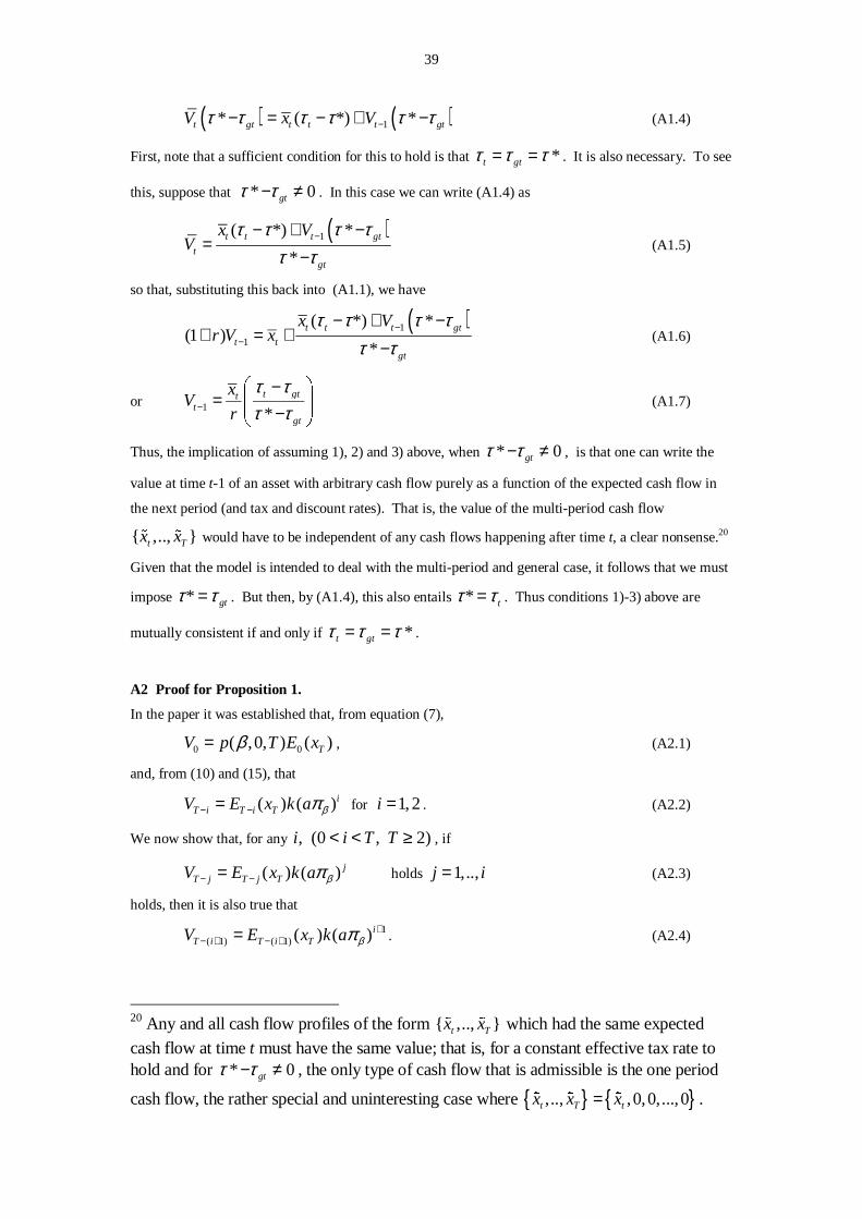
( ) ( )1* ( *) *t gt t t t gtV x Vτ τ τ τ τ τ−− = − + − (A1.4)

First, note that a sufficient condition for this to hold is that *t gtτ τ τ= = . It is also necessary. To see

this, suppose that * 0gtτ τ− ≠ . In this case we can write (A1.4) as

( )1( *) *

*t t t gt

tgt

x VV

τ τ τ ττ τ

−− + −=

− (A1.5)

so that, substituting this back into (A1.1), we have

( )1

1

( * ) *(1 )

*t t t gt

t tgt

x Vr V x

τ τ τ ττ τ

−−

− + −+ = +

− (A1.6)

or 1 *t gtt

tgt

xV

r

τ ττ τ−

� �−

= � �� �−� � (A1.7)

Thus, the implication of assuming 1), 2) and 3) above, when * 0gtτ τ− ≠ , is that one can write the

value at time t-1 of an asset with arbitrary cash flow purely as a function of the expected cash flow in

the next period (and tax and discount rates). That is, the value of the multi-period cash flow

{ ,.., }t Tx x���

would have to be independent of any cash flows happening after time t, a clear nonsense.20

Given that the model is intended to deal with the multi-period and general case, it follows that we must

impose * gtτ τ= . But then, by (A1.4), this also entails * tτ τ= . Thus conditions 1)-3) above are

mutually consistent if and only if *t gtτ τ τ= = .

A2 Proof for Proposition 1.

In the paper it was established that, from equation (7),

0 0( ,0, ) ( )TV p T E xβ= , (A2.1)

and, from (10) and (15), that

( ) ( )iT i T i TV E x k a βπ− −= for 1,2i = . (A2.2)

We now show that, for any , (0 , 2)i i T T< < ≥ , if

( ) ( ) jT j T j TV E x k a βπ− −= holds 1,..,j i= (A2.3)

holds, then it is also true that

1( 1) ( 1) ( ) ( )i

T i T i TV E x k a βπ +− + − += . (A2.4)

20 Any and all cash flow profiles of the form { ,.., }t Tx x

��� which had the same expected

cash flow at time t must have the same value; that is, for a constant effective tax rate to hold and for * 0gtτ τ− ≠ , the only type of cash flow that is admissible is the one period

cash flow, the rather special and uninteresting case where { } { },.., ,0,0,...,0t T tx x x=�

.

40

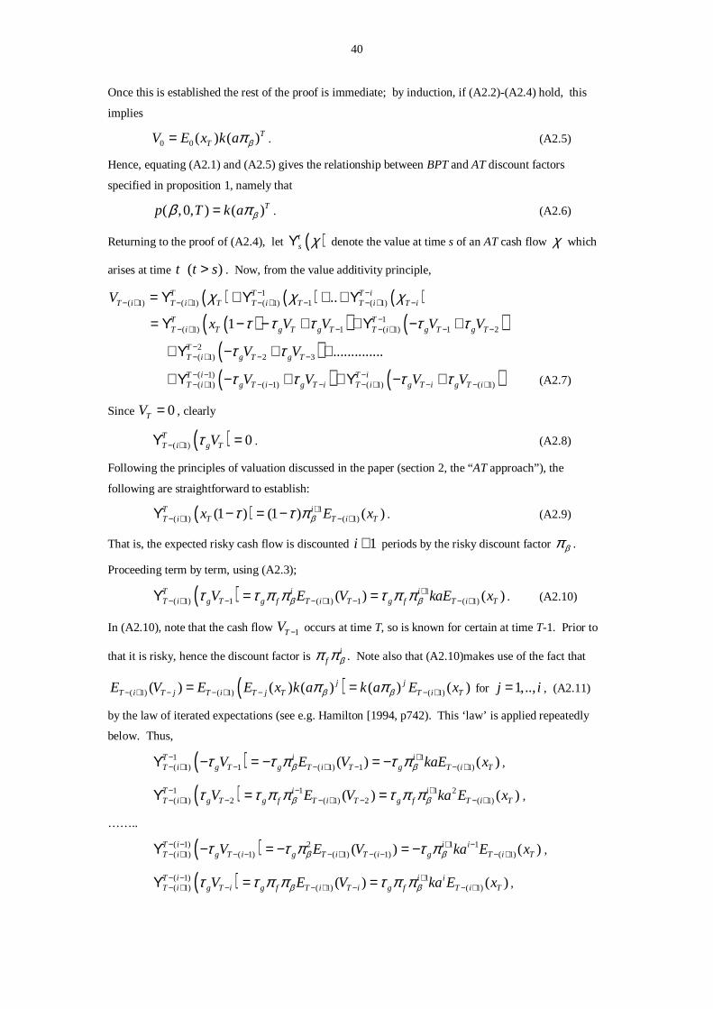
Once this is established the rest of the proof is immediate; by induction, if (A2.2)-(A2.4) hold, this

implies

0 0( ) ( )TTV E x k a βπ= . (A2.5)

Hence, equating (A2.1) and (A2.5) gives the relationship between BPT and AT discount factors

specified in proposition 1, namely that

( ,0, ) ( )Tp T k a ββ π= . (A2.6)

Returning to the proof of (A2.4), let ( )ts χϒ denote the value at time s of an AT cash flow χ which

arises at time ( )t t s> . Now, from the value additivity principle,

( ) ( ) ( )( )( ) ( )

( )( )

1( 1) ( 1) ( 1) 1 ( 1)

1( 1) 1 ( 1) 1 2

2( 1) 2 3

( 1)( 1) ( 1) ( 1)

..

1

..............

T T T iT i T i T T i T T i T i

T TT i T g T g T T i g T g T

TT i g T g T

T i T iT i g T i g T i T i g T

V

x V V V V

V V

V V V

χ χ χ

τ τ τ τ τ

τ τ

τ τ τ

− −− + − + − + − − + −

−− + − − + − −

−− + − −

− − −− + − − − − +

= ϒ + ϒ + + ϒ

= ϒ − − + + ϒ − +

+ ϒ − + +

+ ϒ − + + ϒ −( )( 1)i g T iVτ− − ++ (A2.7)

Since 0TV = , clearly

( )( 1) 0TT i g TVτ− +ϒ = . (A2.8)

Following the principles of valuation discussed in the paper (section 2, the “AT approach” ), the

following are straightforward to establish:

( ) 1( 1) ( 1)(1 ) (1 ) ( )T i

T i T T i Tx E xβτ τ π +− + − +ϒ − = − . (A2.9)

That is, the expected risky cash flow is discounted 1i + periods by the risky discount factor βπ .

Proceeding term by term, using (A2.3);

( ) 1( 1) 1 ( 1) 1 ( 1)( ) ( )T i i

T i g T g f T i T g f T i TV E V kaE xβ βτ τ π π τ π π +− + − − + − − +ϒ = = . (A2.10)

In (A2.10), note that the cash flow 1TV − occurs at time T, so is known for certain at time T-1. Prior to

that it is risky, hence the discount factor is if βπ π . Note also that (A2.10)makes use of the fact that

( )( 1) ( 1) ( 1)( ) ( ) ( ) ( ) ( )j jT i T j T i T j T T i TE V E E x k a k a E xβ βπ π− + − − + − − += = for 1,..,j i= , (A2.11)

by the law of iterated expectations (see e.g. Hamilton [1994, p742). This ‘ law’ is applied repeatedly

below. Thus,

( )1 1( 1) 1 ( 1) 1 ( 1)( ) ( )T i i

T i g T g T i T g T i TV E V kaE xβ βτ τ π τ π− +− + − − + − − +ϒ − = − = − ,

( )1 1 1 2( 1) 2 ( 1) 2 ( 1)( ) ( )T i i

T i g T g f T i T g f T i TV E V ka E xβ βτ τ π π τ π π− − +− + − − + − − +ϒ = = ,

……..

( )( 1) 2 1 1( 1) ( 1) ( 1) ( 1) ( 1)( ) ( )T i i i

T i g T i g T i T i g T i TV E V ka E xβ βτ τ π τ π− − + −− + − − − + − − − +ϒ − = − = − ,

( )( 1) 1( 1) ( 1) ( 1)( ) ( )T i i i

T i g T i g f T i T i g f T i TV E V ka E xβ βτ τ π π τ π π− − +− + − − + − − +ϒ = = ,

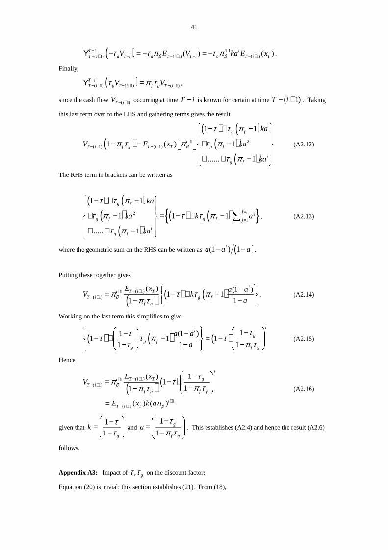
41

( ) 1( 1) ( 1) ( 1)( ) ( )T i i i

T i g T i g T i T i g T i TV E V ka E xβ βτ τ π τ π− +− + − − + − − +ϒ − = − = − .

Finally,

( )( 1) ( 1) ( 1)T iT i g T i f g T iV Vτ π τ−

− + − + − +ϒ = ,

since the cash flow ( 1)T iV − + occurring at time T i− is known for certain at time ( 1)T i− + . Taking

this last term over to the LHS and gathering terms gives the result

( )( ) ( )

( )( )

1 2( 1) ( 1)

1 1

1 ( ) 1

....... 1

g f

iT i f g T i T g f

ig f

ka

V E x ka

ka

β

τ τ π

π τ π τ π

τ π

+− + − +

� �− + −� �� ����

− = + −� ��� � �

+ + −� � �

(A2.12)

The RHS term in brackets can be written as

( ) ( )( )

( )( ) ( ){ }2

1

1 1

1 1 1

...... 1

g f

j i jg f g f j

ig f

ka

ka k a

ka

τ τ π

τ π τ τ π

τ π

=

=

� − + −� �� �

+ − = − + −� �� �+ + −� �� �

�, (A2.13)

where the geometric sum on the RHS can be written as ( )(1 ) 1ia a a− − .

Putting these together gives

( ) ( ) ( )( 1)1( 1)

( ) (1 )1 1

11

iT i Ti

T i g f

f g

E x a aV k

aβπ τ τ ππ τ

− ++− +

� �−= − + −

� �−− � � . (A2.14)

Working on the last term this simplifies to give

( ) ( ) ( ) 11 (1 )1 1 1

1 1 1

ii

gg f

g f g

a a

a

τττ τ π ττ π τ

� ���� � �−− −

� �− + − = − ! !" # ! !

− − −� �$�% $ %& ' (A2.15)

Hence

( ) ( )( 1)1( 1)

1( 1)

( ) 11

11

( ) ( )

i

T i T giT i

f gf g

iT i T

E xV

E x k a

β

β

τπ τ

π τπ τ

π

− ++− +

+− +

( )−

= − * +* +−− , -=

(A2.16)

given that 1

1 g

kττ

.0/−= 1 21 2−304 and

1

1g

f g

aτ

π τ

5 6−

= 7 87 8−9 : . This establishes (A2.4) and hence the result (A2.6)

follows.

Appendix A3: Impact of , gτ τ on the discount factor:

Equation (20) is trivial; this section establishes (21). From (18),

42

( ) ( )( )

T

gf

g

g

Tp ���

����

�

−−

���

����

�

−−=

τπτ

πττβ β 1

1

1

1,0, . (A3.1)

The partial derivative with respect to gτ is given as (using the product, chain and quotient rules):

( ) ( )( )

( ) ( ) ( ) ( )( )

1 1

2

,0, ,0,

1

1 1 1 111 1

g g

T T T T

g f g f f g gT

Tg f g

p T p T

T Tβ

β βτ τ

τ π τ π π τ ττ πτ π τ

− −

∂=

∂ −� �

− − − + − −���

− + − −��� � �

(A3.2)

which can be simplified to give

( ) ( ) ( ) ( )( )( )( )

,0, 1 1,0,

1 1

f g f

g g f g

p T Tp T β π τ πβτ τ π τ

− − −∂=

∂ − −

(A3.3)

which is equation (21) in the paper.