Aprismatic Beams – A Mathematical Model and Application to

Aprismatic Beams – A Mathematical Model and Application to a One Kilometre Arch Bridge

John Nichols

Department of Construction Science, College of Architecture, Texas A&M University, College Station, United States

Email: [email protected]

Abstract. Design engineers, like all humans, are driven by Nash game theory to maximize return and hence simplify design. A determination of the optimal shape of beams to maximize strength and minimize costs has been an area of significant research since the 1970’s. However, real cost constraints in the market place usually see the selection of standard beams with invariant inertia tensor properties being used for most buildings throughout the world. The more challenging problem is the development of a beam of varying cross sectional area, this type of beam provides savings in terms of the quantity of steel and the mass of the ultimate building or bridge without degrading safety and can when manufactured in quantity to reduce costs. The purpose of the paper is to outline the mathematical development of aprismatic beams for everyday use in engineering to reduce material usage and hence human impact on the global environment. An example is provided using a 1 km arch bridge.

Keywords: Aprismatic, beams, Finite elements, arch bridge

1 Introduction

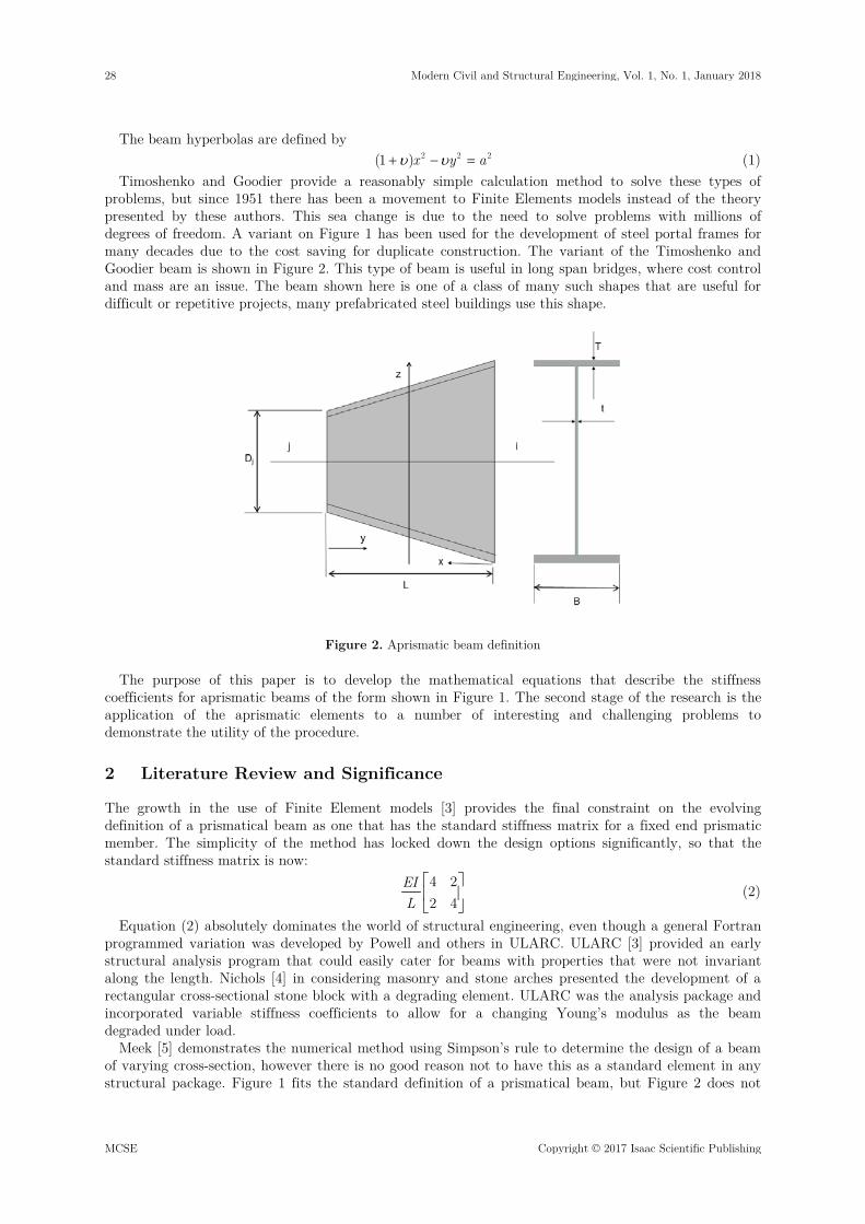
Engineering design for steel and concrete typically uses beams of constant cross-section. Engineering design for masonry beams does not require constant cross-section as the beams are made from small units often by hand. Standard engineering design often uses beams termed prismatic, which has a stricter definition than the optical prism in terms of shape, requiring a beam of constant cross-section and thus invariant inertia tensor properties. The OED [1] defines a prism as “ a solid figure of which the two ends are similar and equal and parallel rectilinear and the sides are parallelograms”. Timoshenko and Goodier [2] provide a reasonably simple definition of prismatical beam with a series of examples in their classic book. Figure 1 shows one example from Timoshenko and Goodier, in this case two parallel vertical sides and two hyperbolas. Modern structural analysis thought is based on this model of beam, although the beam here is probably too costly to construct for all but the most special uses.

Figure 1. Prismatic beam from Timoshenko and Goodier (1951).

Modern Civil and Structural Engineering, Vol. 1, No. 1, January 2018 https://dx.doi.org/10.22606/mcse.2017.11003 27

Copyright © 2017 Isaac Scientific Publishing MCSE

The beam hyperbolas are defined by υ υ+ − =2 2 2(1 )x y a (1)

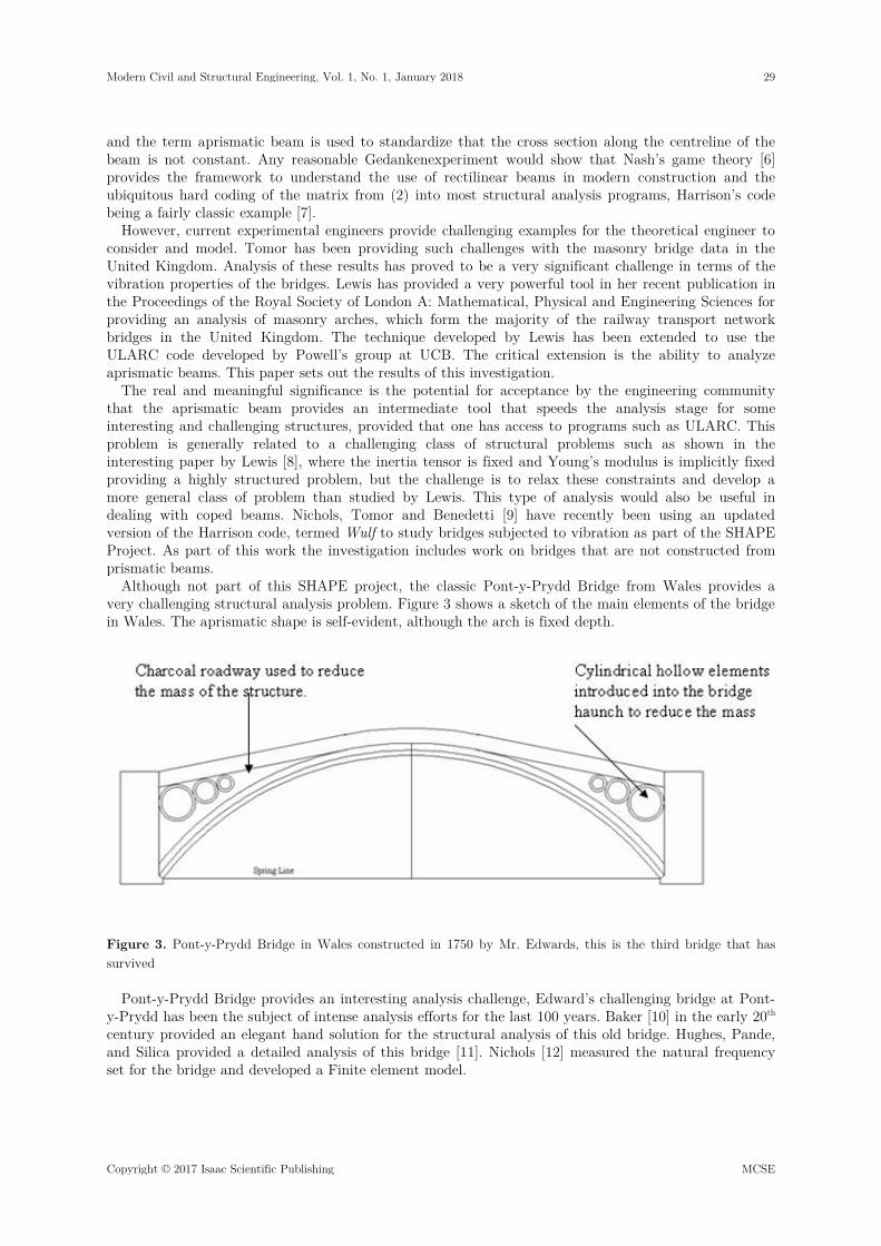
Timoshenko and Goodier provide a reasonably simple calculation method to solve these types of problems, but since 1951 there has been a movement to Finite Elements models instead of the theory presented by these authors. This sea change is due to the need to solve problems with millions of degrees of freedom. A variant on Figure 1 has been used for the development of steel portal frames for many decades due to the cost saving for duplicate construction. The variant of the Timoshenko and Goodier beam is shown in Figure 2. This type of beam is useful in long span bridges, where cost control and mass are an issue. The beam shown here is one of a class of many such shapes that are useful for difficult or repetitive projects, many prefabricated steel buildings use this shape.

Figure 2. Aprismatic beam definition

The purpose of this paper is to develop the mathematical equations that describe the stiffness coefficients for aprismatic beams of the form shown in Figure 1. The second stage of the research is the application of the aprismatic elements to a number of interesting and challenging problems to demonstrate the utility of the procedure.

2 Literature Review and Significance

The growth in the use of Finite Element models [3] provides the final constraint on the evolving definition of a prismatical beam as one that has the standard stiffness matrix for a fixed end prismatic member. The simplicity of the method has locked down the design options significantly, so that the standard stiffness matrix is now:

4 22 4

EIL

(2)

Equation (2) absolutely dominates the world of structural engineering, even though a general Fortran programmed variation was developed by Powell and others in ULARC. ULARC [3] provided an early structural analysis program that could easily cater for beams with properties that were not invariant along the length. Nichols [4] in considering masonry and stone arches presented the development of a rectangular cross-sectional stone block with a degrading element. ULARC was the analysis package and incorporated variable stiffness coefficients to allow for a changing Young’s modulus as the beam degraded under load.

Meek [5] demonstrates the numerical method using Simpson’s rule to determine the design of a beam of varying cross-section, however there is no good reason not to have this as a standard element in any structural package. Figure 1 fits the standard definition of a prismatical beam, but Figure 2 does not

28 Modern Civil and Structural Engineering, Vol. 1, No. 1, January 2018

MCSE Copyright © 2017 Isaac Scientific Publishing

and the term aprismatic beam is used to standardize that the cross section along the centreline of the beam is not constant. Any reasonable Gedankenexperiment would show that Nash’s game theory [6] provides the framework to understand the use of rectilinear beams in modern construction and the ubiquitous hard coding of the matrix from (2) into most structural analysis programs, Harrison’s code being a fairly classic example [7].

However, current experimental engineers provide challenging examples for the theoretical engineer to consider and model. Tomor has been providing such challenges with the masonry bridge data in the United Kingdom. Analysis of these results has proved to be a very significant challenge in terms of the vibration properties of the bridges. Lewis has provided a very powerful tool in her recent publication in the Proceedings of the Royal Society of London A: Mathematical, Physical and Engineering Sciences for providing an analysis of masonry arches, which form the majority of the railway transport network bridges in the United Kingdom. The technique developed by Lewis has been extended to use the ULARC code developed by Powell’s group at UCB. The critical extension is the ability to analyze aprismatic beams. This paper sets out the results of this investigation.

The real and meaningful significance is the potential for acceptance by the engineering community that the aprismatic beam provides an intermediate tool that speeds the analysis stage for some interesting and challenging structures, provided that one has access to programs such as ULARC. This problem is generally related to a challenging class of structural problems such as shown in the interesting paper by Lewis [8], where the inertia tensor is fixed and Young’s modulus is implicitly fixed providing a highly structured problem, but the challenge is to relax these constraints and develop a more general class of problem than studied by Lewis. This type of analysis would also be useful in dealing with coped beams. Nichols, Tomor and Benedetti [9] have recently been using an updated version of the Harrison code, termed Wulf to study bridges subjected to vibration as part of the SHAPE Project. As part of this work the investigation includes work on bridges that are not constructed from prismatic beams.

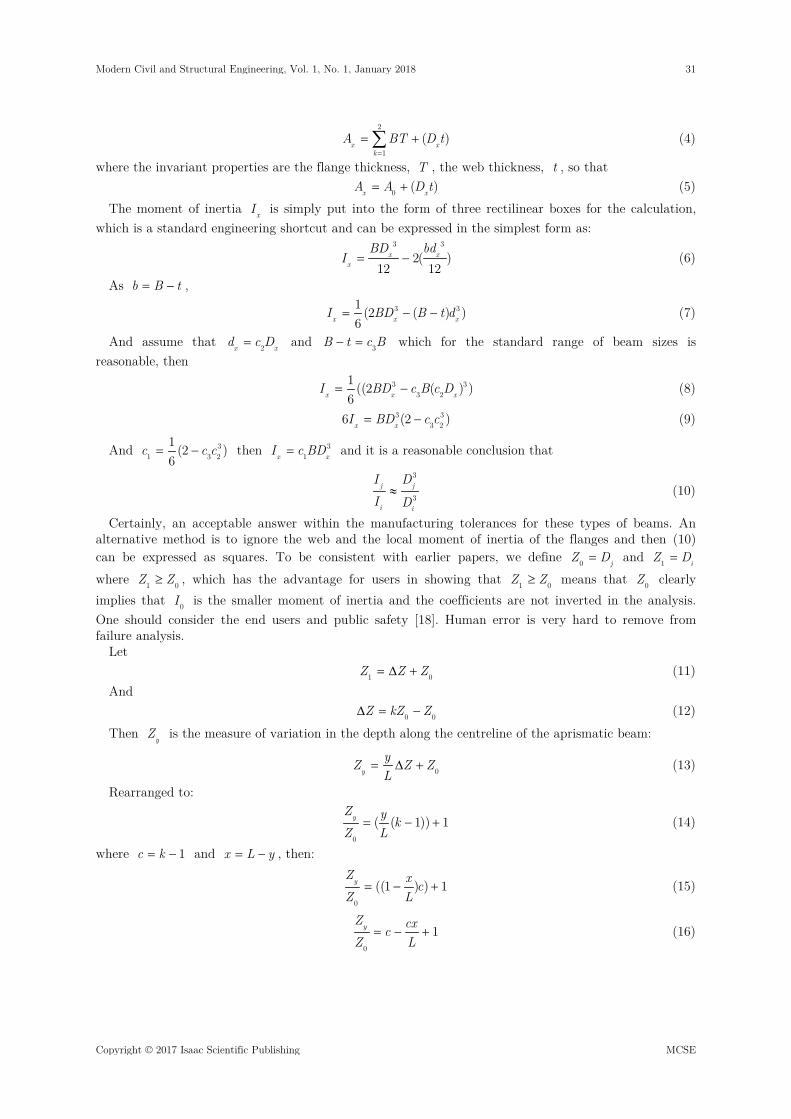
Although not part of this SHAPE project, the classic Pont-y-Prydd Bridge from Wales provides a very challenging structural analysis problem. Figure 3 shows a sketch of the main elements of the bridge in Wales. The aprismatic shape is self-evident, although the arch is fixed depth.

Figure 3. Pont-y-Prydd Bridge in Wales constructed in 1750 by Mr. Edwards, this is the third bridge that has survived

Pont-y-Prydd Bridge provides an interesting analysis challenge, Edward’s challenging bridge at Pont-y-Prydd has been the subject of intense analysis efforts for the last 100 years. Baker [10] in the early 20th century provided an elegant hand solution for the structural analysis of this old bridge. Hughes, Pande, and Silica provided a detailed analysis of this bridge [11]. Nichols [12] measured the natural frequency set for the bridge and developed a Finite element model.

Modern Civil and Structural Engineering, Vol. 1, No. 1, January 2018 29


Lewis in the paper recently published in Proceedings of the Royal Society of London A: Mathematical, Physical and Engineering Sciences has made a significant advance in understanding the methods of vibration analysis for arch and by extension other challenging structures. This interesting analysis on the optimal shapes of arches was developed using a moment-less arch as the key example, although an infinite series of arch shapes and loads can be analyzed using this technique not just the singular one used by Lewis. Professor Lewis’ work provides an interesting model to consider the application of aprismatic beam elements. The simplicity of the model belies the power of this technique in developing the next iteration in an arch bridge to 1 kilometer. The arch method recently developed by Lewis to separate the beam and roadway loads provides the essential method to explain the failure mode of the second Edward’s bridge and also explain why the third bridge has survived almost 260 years.

Benedetti et. al., [13] provides a sophisticated analysis of a masonry bridge constructed about 1815 in Northern Italy. The design team for the bridge used the open hydraulic tubes first used by Edwards to reduce the haunch mass, increase the water way area in a controlled manner and break up the lower frequency modes that are problematic for long span masonry bridges, a useful construct in a seismic area, which Parma is.

This current work builds on the recent vibration analysis being completed by Tomor on a number of railway bridges in the UK for the West Somerset railway [14]. In terms of the research interest for the research group that I am a part of, the key elements are the dynamic analysis of bridge structures, and whilst it is simple to use programs such as Strand7 [15], the overwhelming tendency is to move to solid Finite Elements solid elements such as 8 node elements which provide a very long input and analysis stage and results that can be difficult to interpret [16]. The analysis of the Finite Element results is problematic from a design standpoint.

The extension to the current theory is this research is the development of a formal set of stiffness coefficient that will allow the modelling of aprismatic beams without using the numerical integration methods outlined in standard textbooks. In the limit the aprismatic beam approaches the prismatic beam of Timoshenko and Goodier as the slope along the beam surface approaches zero. Of course, it can be easily argued that this is a simple extension of the calculus of beam theory, and to some extent this is correct, the interest here is in the range of applications particularly the vexing issue of long span bridges and the rather simplistic current design methods used for some of these bridges.

3 Analysis and Results

3.1 Structural Model

Figure 2 shows the general configuration of the proposed beam used for this analysis. The variables used in the definition shown in Figure 2 are, L being the element length, ,i j representing the node numbers used in the structural model, usually integers of the form 1,2,3…, z being the vertical axis, x the length from the deeper end of the beam and y the length from the narrow end of the beam. B is the beam width and jD is the beam depth at end j . This beam type represents a potential knee joint for use with standard Universal Beams [17].

This is the general form of a steel beam, although it will work with a concrete beam of the same shape or a masonry beam of varied shape as long as the variation is linear in the depth along the centreline of the beam. This is a much broader problem than covered in the standard text books or used in most Finite Element analysis packages for standard beams.

A standard structural analysis package, such as developed by Harrison [7], provides for the Lewis model of a prismatic beam, but the program developed by Sudhakar and others [3] provides a more general system in this case termed the Powell model for an aprismatic beam. In developing the Lewis model, the standard equations for structural action reduce to an axial force, T , a beam length of L , the invariant property A, the Young’s modulus E and the change in length ∆L :

= ∆AET LL

(3)

In the Powell model the area properties, measured with x along the centreline are generalized to:



=

= +∑2

1( )x x

kA BT D t (4)

where the invariant properties are the flange thickness, T , the web thickness, t , so that = +0 ( )x xA A D t (5)

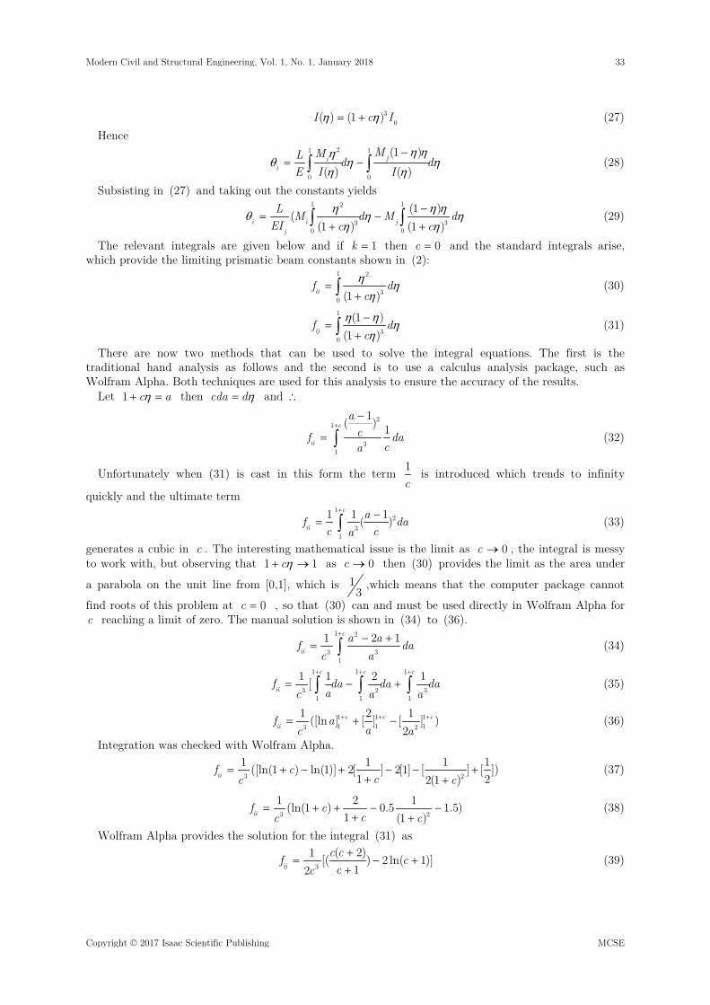
The moment of inertia xI is simply put into the form of three rectilinear boxes for the calculation, which is a standard engineering shortcut and can be expressed in the simplest form as:

= −3 3

2( )12 12

x xx

BD bdI (6)

As = −b B t ,

= − −3 31 (2 ( ) )6x x xI BD B t d (7)

And assume that = 2x xd c D and − = 3B t c B which for the standard range of beam sizes is reasonable, then

= −3 33 2

1 ((2 ( ) )6x x xI BD c B c D (8)

= −3 33 26 (2 )x xI BD c c (9)

And = − 31 3 2

1 (2 )6

c c c then = 31x xI c BD and it is a reasonable conclusion that

≈3

3j j

i i

I DI D

(10)

Certainly, an acceptable answer within the manufacturing tolerances for these types of beams. An alternative method is to ignore the web and the local moment of inertia of the flanges and then (10) can be expressed as squares. To be consistent with earlier papers, we define =0 jZ D and =1 iZ D where ≥1 0Z Z , which has the advantage for users in showing that ≥1 0Z Z means that 0Z clearly implies that 0I is the smaller moment of inertia and the coefficients are not inverted in the analysis. One should consider the end users and public safety [18]. Human error is very hard to remove from failure analysis.

Let = ∆ +1 0Z Z Z (11)

And ∆ = −0 0Z kZ Z (12)

Then yZ is the measure of variation in the depth along the centreline of the aprismatic beam:

= ∆ + 0yyZ Z ZL

(13)

Rearranged to:

= − +0

( ( 1)) 1yZ y kZ L

(14)

where = − 1c k and = −x L y , then:

= − +0

((1 ) ) 1yZ x cZ L

(15)

= − +0

1yZ cxcZ L

(16)



= −0

yZ cxkZ L

(17)

Hence:

=3

1 13

0 0

I ZI Z

(18)

∴

−

=0

31

0 0

( )( )

cxZ kI LI Z

(19)

= − 31

0

( )I cxkI L

(20)

The stiffness matrix for this beam is then

θθ

=

( ) ii iji i

j jji jj

k kM EI yM L k k

(21)

The inverse of the stiffness matrix Κ is the influence matrix Ι and for unit loads and moments the general equation is shown in (22)

−

= −

∫11 120

21 22

1 1 1L

xf f x xL dxf f EI L Lx

L

(22)

Then the individual matrix Ι elements can be determined for a general load.

θ = ∫0

1( )

L

iM ydy

L EI y (23)

The relationship between the end moments and M is shown in Figure 4.

Figure 4. Moment diagram

And from Figure 4 the moment variation along the centreline of the aprismatic beam is:

= − −( ) (1 )y i jy yM M ML L

(24)

θ =−

−∫

300

1( )( )

L

iM ydy

L c L yEI kL

(25)

And substituting (24) into (25) and using η =yL

yields

θ η ηη

= ∫1

0

1 ( )( )iM L Ld

EL I (26)

∴ from (20)



η η= + 30( ) (1 )I c I (27)

Hence

η ηη

θ η ηη η

−= −∫ ∫

21 1

0 0

(1 )( ) ( )

jii

MML d dE I I

(28)

Subsisting in (27) and taking out the constants yields

η ηηθ η ηη η

−= −

+ +∫ ∫1 12

3 30 0

(1 )((1 ) (1 )i i j

j

L M d M dEI c c

(29)

The relevant integrals are given below and if = 1k then = 0c and the standard integrals arise, which provide the limiting prismatic beam constants shown in (2):

η ηη

=+∫

1 2

30 (1 )iif d

c (30)

η ηη

η−

=+∫

1

30

(1 )(1 )ijf d

c (31)

There are now two methods that can be used to solve the integral equations. The first is the traditional hand analysis as follows and the second is to use a calculus analysis package, such as Wolfram Alpha. Both techniques are used for this analysis to ensure the accuracy of the results.

Let η+ =1 c a then η=cda d and ∴

+

−

= ∫2

1

31

1( ) 1c

ii

acf da

ca (32)

Unfortunately when (31) is cast in this form the term 1c

is introduced which trends to infinity

quickly and the ultimate term

+ −

= ∫1

23

1

1 1 1( )c

iiaf da

c ca (33)

generates a cubic in c . The interesting mathematical issue is the limit as → 0c , the integral is messy to work with, but observing that η+ →1 1c as → 0c then (30) provides the limit as the area under

a parabola on the unit line from [0,1], which is 13 ,which means that the computer package cannot

find roots of this problem at = 0c , so that (30) can and must be used directly in Wolfram Alpha for c reaching a limit of zero. The manual solution is shown in (34) to (36).

+ − +

= ∫1 2

3 31

1 2 1c

iia af da

c a (34)

+ + +

= − +∫ ∫ ∫1 1 1

3 2 31 1 1

1 1 2 1[c c c

iif da da daac a a

(35)

+ + += + −1 1 11 1 13 2

1 2 1([ln ] [ ] [ ] )2

c c ciif a

ac a (36)

Integration was checked with Wolfram Alpha.

= + − + − − ++ +3 2

1 1 1 1([ln(1 ) ln(1)] 2[ ] 2[1] [ ] [ ])1 22(1 )iif c

cc c (37)

= + + − −+ +3 2

1 2 1(ln(1 ) 0.5 1.5)1 (1 )iif c

cc c (38)

Wolfram Alpha provides the solution for the integral (31) as

+= − +

+3

( 2)1 [( ) 2 ln( 1)]12ij

c cf ccc

(39)



Provided ≠ 0c where the limit is the standard answer for prismatic members at 16 . The jjk term

is trivially:

ηη

η−

=+∫

1 2

30

(1 )(1 )jjf d

c (40)

There are reasonable limits for the range of knee joint beams that can be used in construction. This analysis used a domain for c from 0 to 20.

3.2 Graphical Results

Figure 3 shows a plot of the influence coefficients iif and so on. There are two direct uses for this data, it can be used by a design engineer directly with ULARC or it can be implemented into the program code, which is the proposal for the code developed by Harrison [7], which has been implemented with PARDISO [19], probably the fastest inversion program at the moment and eigenvalue solver FEAST [20], probably the fastest eigenvector solver at the moment and using the methods outlined by Gavin for the dynamic analysis of structures for the Newmark-Beta method [21].

The results are plotted in a logarithm to logarithm space and a trendline is fitted to the data. The trendline is a 6th order polynomial. This selection provides the best fit to the data as shown in Figure 5.

Figure 5. Influence coefficient plotted in a logarithm to logarithm space

Figure 6 shows the results of the matrix inversion of the 2x2 matrices for the flexibility results shown in Figure 5. The results are plotted in log-log space. Several methods of statistical analysis were used on the stiffness coefficient data. The closest fit is obtained with a linear regression analysis in logarithm to logarithm space.

Table 1 provides the results from the linear regression completed using the standard EXCEL linear regression model. It is accepted that the results show more decimal places than warranted by a standard statistical analysis [22], but the data is intended for computer programs and a FORTRAN double



precision can easily handle these numbers and the intent is to replicate the original data as closely as possible with the code.

Table 1. Stiffness Coefficients – Linear Regression Analysis

Moment of Inertia Ratio Equation Component Coefficients Standard Error

Cubic Intercept (a) 0.573165 0.004643 X Variable (b) 0.793823 0.002934

Square Intercept (a) 0.599443 0.000538 X Variable (b) 0.772944 0.001275

Clearly the two sets of results are quite close and the t-Stat numbers were well above those needed to

be statistically significant.

Figure 6. Plot of the logarithm of the ratio of the moments of inertia to logarithm of the stiffness coefficients.

The stiffness coefficients can be used in any program that will accept input of direct stiffness coefficients, such as ULARC [3] from UCB. The examples in this paper will be completed with this elastic-plastic program. Clearly, the question is why we are now interested in an extension to standard beam theory. Even a commonly used FEM package, such as Strand7 requires the direct input of the stiffness coefficients for a member as shown in Figure 2. Figure 7 shows a sample of the input screen. The other consideration is of course the use of shear areas, which has a direct impact on the eigenfrequencies.

3.3 Analysis

There are hundreds of interesting and challenging structural analysis problems investigated in the literature every year. Baker’s classic text [10] provides more than a score, some dating from the 18th century. Lewis’ interesting paper [8] prompted this research paper as one considered the use of Lewis’ technique in the problems identified in some of the problems by Baker. It is also prompted by recent work by Tomor on masonry arch bridges in the UK [23]. A future paper will consider the joint issue of damage to an aprismatic beam.



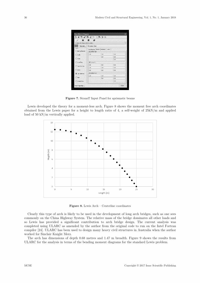
Figure 7. Strand7 Input Panel for aprismatic beams

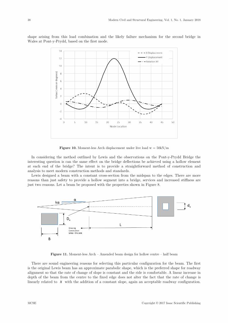
Lewis developed the theory for a moment-less arch. Figure 8 shows the moment free arch coordinates obtained from the Lewis paper for a height to length ratio of 4, a self-weight of 25kN/m and applied load of 50 kN/m vertically applied.

Figure 8. Lewis Arch – Centerline coordinates

Clearly this type of arch is likely to be used in the development of long arch bridges, such as one sees commonly on the China Highway System. The relative mass of the bridge dominates all other loads and so Lewis has provided a significant contribution to arch bridge design. The current analysis was completed using ULARC as amended by the author from the original code to run on the Intel Fortran compiler [24]. ULARC has been used to design many heavy civil structures in Australia when the author worked for Sinclair Knight Merz.

The arch has dimensions of depth 0.68 metres and 1.47 m breadth. Figure 9 shows the results from ULARC for the analysis in terms of the bending moment diagrams for the standard Lewis problem.



Figure 9. Analysis of Lewis Moment-Free-Arch with Powell Beam alternative

The critical line is the solid black line showing the resultant bending stress for the beam, Lewis has achieved her objective within the limits of accuracy of the ULARC and the published numerical numbers. The thin gray line shows the relative error between the flexural stress and the axial stress.

The first load applied to the standard Lewis bridge is the self-weight of the arch, which due to the uniform shape is set at 25 kN/m for the length of the arch, as the Lewis arch has constant cross-section of 1 square meter. The results for this load are shown in Figure 9 as self-weight. The second applied load is the applied roadway load which generated as a constant along the X axis. This load models a road bridge spanning between supports on the arch, a commonly observed design in China on large span motorway bridges. This load shows a bending moment that is exactly opposite and almost equal to the self-weight, on Figure 9 as the applied load. The results are shown in the figure for the two loads as a combined load case listed purely as axial and flexural stress. The small misclose is probably due to the rounding in the data supplied with the paper and the use of spring based restraint points in ULARC instead of fixed restraints as studied by Lewis. Figure 10 shows X and Y displacement for the arch under the roadway load.

The results show an upward thrust by the centre of the bridge under the applied load. This matches the observation by Baker on the failure mode of the Pont-y-Bridge. Edward’s the builder for the Pont-y-Prydd Bridge in developing the third bridge, after the loss of the first two bridges, used two techniques to avoid the upwelling of the centre of the second bridge leading to its failure at the removal of the centreing. The first technique was to use Charcoal as a fill material, with a unit mass closer to the unit of mass of water in place of stone or soil. The second is the introduction of circular empty elements into the haunches as shown on Figure 3. Lewis’s method shows why this worked in 1760. Nichols [25] completed a failure analysis of the Pont-y-Prydd Bridge using ABAQUS and demonstrated the modal



shape arising from this load combination and the likely failure mechanism for the second bridge in Wales at Pont-y-Prydd, based on the first mode.

Figure 10. Moment-less Arch displacement under live load w = 50kN/m

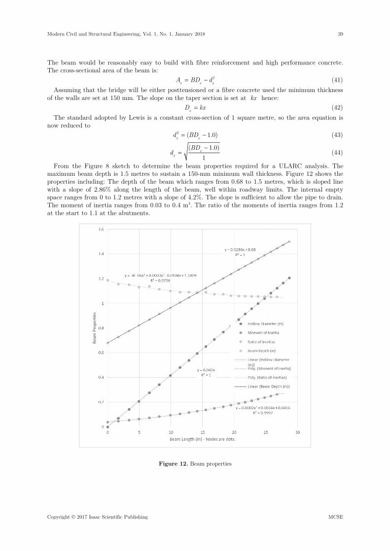
In considering the method outlined by Lewis and the observations on the Pont-y-Prydd Bridge the interesting question is can the same effect on the bridge deflections be achieved using a hollow element at each end of the bridge? The intent is to provide a straightforward method of construction and analysis to meet modern construction methods and standards.

Lewis designed a beam with a constant cross-section from the midspan to the edges. There are more reasons than just safety to provide a hollow segment into a bridge, services and increased stiffness are just two reasons. Let a beam be proposed with the properties shown in Figure 8.

Figure 11. Moment-less Arch – Amended beam design for hollow centre – half beam

There are sound engineering reasons for selecting this particular configuration for the beam. The first is the original Lewis beam has an approximate parabolic shape, which is the preferred shape for roadway alignment so that the rate of change of slope is constant and the ride is comfortable. A linear increase in depth of the beam from the centre to the fixed edge does not alter the fact that the rate of change is linearly related to x with the addition of a constant slope, again an acceptable roadway configuration.



The beam would be reasonably easy to build with fibre reinforcement and high performance concrete. The cross-sectional area of the beam is: = − 2

x x xA BD d (41) Assuming that the bridge will be either posttensioned or a fibre concrete used the minimum thickness

of the walls are set at 150 mm. The slope on the taper section is set at kx hence: =xD kx (42)

The standard adopted by Lewis is a constant cross-section of 1 square metre, so the area equation is now reduced to = −2 ( 1.0)x xd BD (43)

−

=( 1.0)

1x

x

BDd (44)

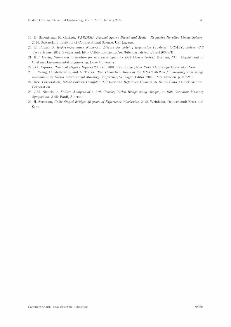
From the Figure 8 sketch to determine the beam properties required for a ULARC analysis. The maximum beam depth is 1.5 metres to sustain a 150-mm minimum wall thickness. Figure 12 shows the properties including: The depth of the beam which ranges from 0.68 to 1.5 metres, which is sloped line with a slope of 2.86% along the length of the beam, well within roadway limits. The internal empty space ranges from 0 to 1.2 metres with a slope of 4.2%. The slope is sufficient to allow the pipe to drain. The moment of inertia ranges from 0.03 to 0.4 m4. The ratio of the moments of inertia ranges from 1.2 at the start to 1.1 at the abutments.

Figure 12. Beam properties



Figure 13. Moment less arch – Powell Beam – Stress Results

Figure 14. Moment less arch – comparison of displacements between original and modified arch

ULARC was used to reanalyze the modified Lewis beam, termed a Powell Beam for the purposes of this paper. The cross-sectional area of the beam has been maintained constant at 1 sqm. Figure 13



shows the stress results for the Powell Beam. The critical results are the axial stress which is a maximum of 4.6 MPa at the abutments and well within the capacity of normal weight concrete. The combined flexural stress is about -0.18 MPa, which given the numerical results provides a close fit to the theoretical system proposed by Lewis.

The results are for the Lewis number for the beam published on the Proceedings of the Royal Society of London A: Mathematical, Physical and Engineering Sciences website, it is likely that recalculating these numbers using Double Precison Fortran [24] would reduce the error further, which is not required to understand the extreme utility of the method developed by Lewis.

Figure 14 shows the displacements for two cases, the Lewis and the Powell beams. The dark blue line shows the Lewis deflections in the Y or critical direction with a peak of 6 mm or thereabouts. The span to deflection ratio is 4600 for the Lewis beam, which shows that the deflection will not cause visible movement on the bridge nor be unacceptable. The Powell beam has a deflection of 3.5 mm, which is a ratio of 9000 or thereabouts, which shows that the beam has acceptable deflections for the applied load.

The stiffer beam reduces the rotations on the ends of the abutments, which are assumed stiff, but not infinitely stiff as is usual when using ULARC.

3.4 A Kilometre Arch Bridge

There are thousands of arch bridges in the world, there is an observed upper limit on the length of arch bridges at 550 metres for a bridge in China built in 2009. Svensson [26] opined in 2014 that the upper cost effective limit for arch bridges is 300 metres as discussed in the introduction to this classic text.

One of course is mindful of the 210 metre bridge that Brunel designed for Bristol as a suspension bridge in the early 19th century, which still stands today. The reasonable research question is:

Can one design a 1000 metre arch bridge in one span? Clearly the purpose of this paper is to consider the development and mathematics of the Powell beam

and that in the scant remaining space, one is not going to answer that question in this paper. But, a suggested starting point is a Powell beam with a span of 1000 metre in an arch configuration with a height say of 250 metres. The likely configuration of the arch is two slanting inward arches meeting at the crown. It is suggested that the hangers for the roadway should be designed to impart a compression into the arch element. This will require a judicious placement of the cables and supports. Figure 15 shows a Rhino sketch for the start of the design.

A second arrangement of cables closer to a cable stayed configuration should also be considered.

Figure 15. Rhino Sketch for a 1000 metre arch bridge



4 Conclusion

This paper sets out the mathematical theory for the development of a simple class of aprismatic beams that could be used in both building and bridge construction. The code can be developed in standard FEM programs to provide a simple and safe implementation.

Lewis provides an interesting conceptual idea for constant cross-section prismatic beams. Her work looks at the Euclidian geometry and the load distribution to arrive at a “theoretical” moment-less arch. In reality, she cancels one moment with the other to arrive at an approximately zero solution. The strength of her work is in the identification of a method for solving a class of optimization problems, although she imposed a very strict limit with prismatic beams and uniform loads. Prismatic beams are common place, but uniform loads are not in highways or railways.

The paper considered an alternative Powell beam which provides for an increase in the moment of inertia of a Lewis beam without increasing the mass, the structural efficiency is improved at limited costs. A reanalysis of the moment less beam developed by Lewis using the Powell beam, an aprismatic beam, sees a reduction in the peak vertical deflection from 5.5 to 3 mm without an increase in mass and a likely reduction in the quantity of steel as the effective depth rises significantly.

The early thoughts on developing a kilometre-long arch provide some interesting conceptual thoughts on the potential for a large Powell beam. Whether this solution is economic in the long run is one that will be investigated in a future paper, but the point of the arch is to avoid the massive cantilever towers of the cable stayed bridge. The issue of constructability will be the greatest challenge if it is economic.

References

1. W. Little, et al., The Shorter Oxford English Dictionary on Historical Principles. 1973, Oxford: Clarendon Press. 2. S. Timoshenko and J.N. Goodier, Theory of Elasticity. 1951, New York, NY: McGraw-Hill Book Company Inc. 3. A. Sudhakar, et al., Computer Program: ULARC: Sample Elasto-plastic Analysis of Plane Frames. Sudhakar

1972 ed. 1972, Berkeley: UCB. 4. J.M. Nichols, The degrading effective stiffness of masonry finite element model: amendments to allow for a non-

symmetric damage element, in Australian Masonry Conference. 2004: Newcastle, Australia. 5. J.L. Meek, Matrix Structural Analysis. 1971, NY: McGraw. 6. J.F. Nash Jr., Essays on Game Theory. 1996, Cheltenham, UK: Edward Elgar Publishing Limited. 7. H.B. Harrison, Computer Methods in Structural Analysis. 1973, Englewood Cliffs, NJ: Prentice. 8. W.J. Lewis, Mathematical model of a moment-less arch. Proceedings of the Royal Society of London A:

Mathematical, Physical and Engineering Sciences, 2016. 472(2190). 9. A.K. Tomor, J.M. Nichols, and A. Benedetti, Identifying the condition of masonry arch bridges using CX1

accelerometer in Eighth International Conference on Arch Bridges. 2016: Wroclaw, Poland. 10. I.O. Baker, Treatise on Masonry Construction. Baker 1914 ed. 1914, New York: Wiley. xiv+745. 11. T.G. Hughes, G.N. Pande, and C. Sicilia. William Edwards Bridge, Pontypridd. in The South Wales Institute of

Engineers. 1998. University of Glamorgan, Pontypridd. 12. J.M. Nichols, A Modal Study of the Pont-Y-Prydd Bridge using the Variance Method. Masonry International,

2013. 26(2): p. 23-33. 13. A. Benedetti, et al., Taro Bridge in Parma: Studies on a 19th century masonry bridge. 2017, UNIBO: Bologna,

Italy. 14. A. Tomor, Methodology for fatigue life expectancy of masonry arch bridges. 2014, International Union of

Railways (Research Report): Paris. 15. Strand7 Pty. Ltd., Strand 7 Manual. 2009, Perth: Strand7 Pty.Ltd. 16. A. Taliercio, Closed-form expressions for the macroscopic flexural rigidity coefficients of periodic brickwork.

Mechanics Research Communications, 2016. 72: p. 24-32. 17. American Institute of Steel Construction (AISC), Steel Construction Manual 14th Edition. 3rd ed., ed. 2011,

Chicago, IL.: AISC. 18. R.E. Melchers, Structural Reliability. 1987, Chichester: Ellis Horword Limited.



19. O. Schenk and K. Gartner, PARDISO: Parallel Sparse Direct and Multi - Recursive Iterative Linear Solvers. 2014, Switzerland: Institute of Computational Science, USI Lugano.

20. E. Polizzi, A High-Performance Numerical Library for Solving Eigenvalue Problems: {FEAST} Solver v2.0 User's Guide. 2012, Switzerland: http://dblp.uni-trier.de/rec/bib/journals/corr/abs-1203-4031.

21. H.P. Gavin, Numerical integration for structural dynamics (541 Course Notes). Durham, NC. : Department of Civil and Environmental Engineering, Duke University.

22. G.L. Squires, Practical Physics. Squires 2001 ed. 2001, Cambridge ; New York: Cambridge University Press. 23. J. Wang, C. Melbourne, and A. Tomor, The Theoretical Basis of the MEXE Method for masonry arch bridge

assessment, in Eighth International Masonry Conference, W. Jager, Editor. 2010, IMS: Dresden. p. 207-216. 24. Intel Corporation, Intel® Fortran Compiler 16.0 User and Reference Guide 2016, Santa Clara, California: Intel

Corporation. 25. J.M. Nichols, A Failure Analysis of a 17th Century Welsh Bridge using Abaqus, in 10th Canadian Masonry

Symposium. 2005: Banff, Alberta. 26. H. Svensson, Cable Stayed Bridges 40 years of Experience Worldwide. 2012, Weinheim, Deutschland: Ernst and

Sohn.



http://dblp.uni-trier.de/rec/bib/journals/corr/abs-1203-4031

Documents

Aprismatic Beams – A Mathematical Model and Application to