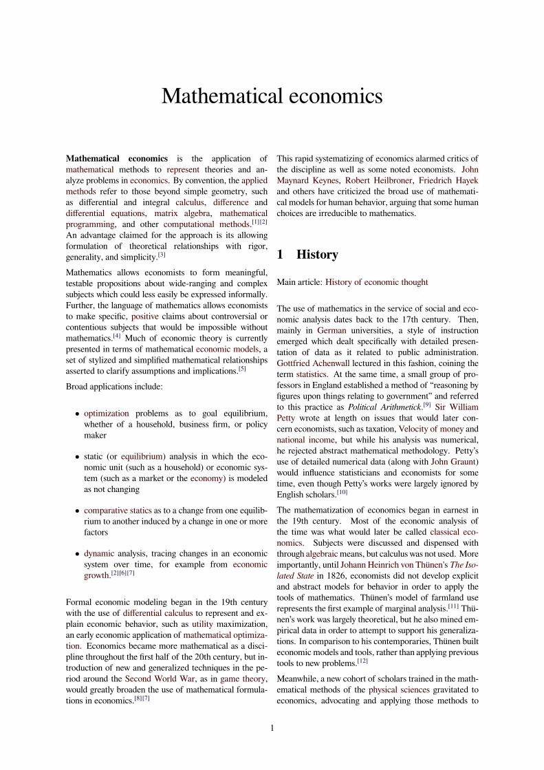
Mathematical economics

Mathematical economics is the application ofmathematical methods to represent theories and an-alyze problems in economics. By convention, the appliedmethods refer to those beyond simple geometry, suchas differential and integral calculus, difference anddifferential equations, matrix algebra, mathematicalprogramming, and other computational methods.[1][2]An advantage claimed for the approach is its allowingformulation of theoretical relationships with rigor,generality, and simplicity.[3]

Mathematics allows economists to form meaningful,testable propositions about wide-ranging and complexsubjects which could less easily be expressed informally.Further, the language of mathematics allows economiststo make specific, positive claims about controversial orcontentious subjects that would be impossible withoutmathematics.[4] Much of economic theory is currentlypresented in terms of mathematical economic models, aset of stylized and simplified mathematical relationshipsasserted to clarify assumptions and implications.[5]

Broad applications include:

• optimization problems as to goal equilibrium,whether of a household, business firm, or policymaker

• static (or equilibrium) analysis in which the eco-nomic unit (such as a household) or economic sys-tem (such as a market or the economy) is modeledas not changing

• comparative statics as to a change from one equilib-rium to another induced by a change in one or morefactors

• dynamic analysis, tracing changes in an economicsystem over time, for example from economicgrowth.[2][6][7]

Formal economic modeling began in the 19th centurywith the use of differential calculus to represent and ex-plain economic behavior, such as utility maximization,an early economic application of mathematical optimiza-tion. Economics became more mathematical as a disci-pline throughout the first half of the 20th century, but in-troduction of new and generalized techniques in the pe-riod around the Second World War, as in game theory,would greatly broaden the use of mathematical formula-tions in economics.[8][7]

This rapid systematizing of economics alarmed critics ofthe discipline as well as some noted economists. JohnMaynard Keynes, Robert Heilbroner, Friedrich Hayekand others have criticized the broad use of mathemati-cal models for human behavior, arguing that some humanchoices are irreducible to mathematics.

1 History

Main article: History of economic thought

The use of mathematics in the service of social and eco-nomic analysis dates back to the 17th century. Then,mainly in German universities, a style of instructionemerged which dealt specifically with detailed presen-tation of data as it related to public administration.Gottfried Achenwall lectured in this fashion, coining theterm statistics. At the same time, a small group of pro-fessors in England established a method of “reasoning byfigures upon things relating to government” and referredto this practice as Political Arithmetick.[9] Sir WilliamPetty wrote at length on issues that would later con-cern economists, such as taxation, Velocity of money andnational income, but while his analysis was numerical,he rejected abstract mathematical methodology. Petty’suse of detailed numerical data (along with John Graunt)would influence statisticians and economists for sometime, even though Petty’s works were largely ignored byEnglish scholars.[10]

The mathematization of economics began in earnest inthe 19th century. Most of the economic analysis ofthe time was what would later be called classical eco-nomics. Subjects were discussed and dispensed withthrough algebraic means, but calculus was not used. Moreimportantly, until Johann Heinrich von Thünen's The Iso-lated State in 1826, economists did not develop explicitand abstract models for behavior in order to apply thetools of mathematics. Thünen’s model of farmland userepresents the first example of marginal analysis.[11] Thü-nen’s work was largely theoretical, but he also mined em-pirical data in order to attempt to support his generaliza-tions. In comparison to his contemporaries, Thünen builteconomic models and tools, rather than applying previoustools to new problems.[12]

Meanwhile, a new cohort of scholars trained in the math-ematical methods of the physical sciences gravitated toeconomics, advocating and applying those methods to

1

2 1 HISTORY

their subject,[13] and described today as moving fromgeometry to mechanics.[14] These included W.S. Jevonswho presented paper on a “general mathematical the-ory of political economy” in 1862, providing an out-line for use of the theory of marginal utility in politi-cal economy.[15] In 1871, he published The Principles ofPolitical Economy, declaring that the subject as science“must be mathematical simply because it deals with quan-tities.” Jevons expected the only collection of statistics forprice and quantities would permit the subject as presentedto become an exact science.[16] Others preceded and fol-lowed in expanding mathematical representations of eco-nomic problems.

1.1 Marginalists and the roots of neoclas-sical economics

Main article: MarginalismAugustin Cournot and Léon Walras built the tools of the

Reaction functionsq1

q2q2

q1

R2(q1)

R1(q2)

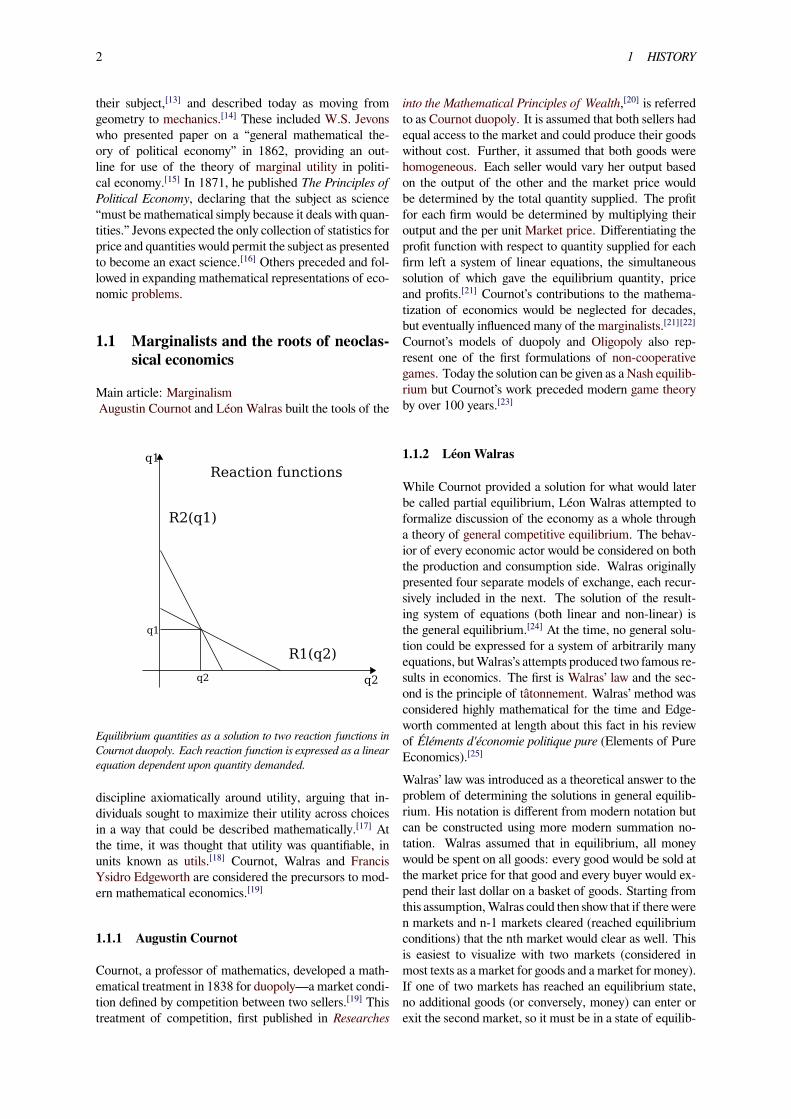
Equilibrium quantities as a solution to two reaction functions inCournot duopoly. Each reaction function is expressed as a linearequation dependent upon quantity demanded.

discipline axiomatically around utility, arguing that in-dividuals sought to maximize their utility across choicesin a way that could be described mathematically.[17] Atthe time, it was thought that utility was quantifiable, inunits known as utils.[18] Cournot, Walras and FrancisYsidro Edgeworth are considered the precursors to mod-ern mathematical economics.[19]

1.1.1 Augustin Cournot

Cournot, a professor of mathematics, developed a math-ematical treatment in 1838 for duopoly—amarket condi-tion defined by competition between two sellers.[19] Thistreatment of competition, first published in Researches

into the Mathematical Principles of Wealth,[20] is referredto as Cournot duopoly. It is assumed that both sellers hadequal access to the market and could produce their goodswithout cost. Further, it assumed that both goods werehomogeneous. Each seller would vary her output basedon the output of the other and the market price wouldbe determined by the total quantity supplied. The profitfor each firm would be determined by multiplying theiroutput and the per unit Market price. Differentiating theprofit function with respect to quantity supplied for eachfirm left a system of linear equations, the simultaneoussolution of which gave the equilibrium quantity, priceand profits.[21] Cournot’s contributions to the mathema-tization of economics would be neglected for decades,but eventually influenced many of the marginalists.[21][22]Cournot’s models of duopoly and Oligopoly also rep-resent one of the first formulations of non-cooperativegames. Today the solution can be given as a Nash equilib-rium but Cournot’s work preceded modern game theoryby over 100 years.[23]

1.1.2 Léon Walras

While Cournot provided a solution for what would laterbe called partial equilibrium, Léon Walras attempted toformalize discussion of the economy as a whole througha theory of general competitive equilibrium. The behav-ior of every economic actor would be considered on boththe production and consumption side. Walras originallypresented four separate models of exchange, each recur-sively included in the next. The solution of the result-ing system of equations (both linear and non-linear) isthe general equilibrium.[24] At the time, no general solu-tion could be expressed for a system of arbitrarily manyequations, butWalras’s attempts produced two famous re-sults in economics. The first is Walras’ law and the sec-ond is the principle of tâtonnement. Walras’ method wasconsidered highly mathematical for the time and Edge-worth commented at length about this fact in his reviewof Éléments d'économie politique pure (Elements of PureEconomics).[25]

Walras’ law was introduced as a theoretical answer to theproblem of determining the solutions in general equilib-rium. His notation is different from modern notation butcan be constructed using more modern summation no-tation. Walras assumed that in equilibrium, all moneywould be spent on all goods: every good would be sold atthe market price for that good and every buyer would ex-pend their last dollar on a basket of goods. Starting fromthis assumption,Walras could then show that if there weren markets and n-1 markets cleared (reached equilibriumconditions) that the nth market would clear as well. Thisis easiest to visualize with two markets (considered inmost texts as a market for goods and a market for money).If one of two markets has reached an equilibrium state,no additional goods (or conversely, money) can enter orexit the second market, so it must be in a state of equilib-

3

rium as well. Walras used this statement tomove toward aproof of existence of solutions to general equilibrium butit is commonly used today to illustrate market clearing inmoney markets at the undergraduate level.[26]

Tâtonnement (roughly, French for groping toward) wasmeant to serve as the practical expression of Walrasiangeneral equilibrium. Walras abstracted the marketplaceas an auction of goods where the auctioneer would callout prices and market participants would wait until theycould each satisfy their personal reservation prices for thequantity desired (remembering here that this is an auctionon all goods, so everyone has a reservation price for theirdesired basket of goods).[27]

Only when all buyers are satisfied with the given marketprice would transactions occur. Themarket would “clear”at that price—no surplus or shortage would exist. Theword tâtonnement is used to describe the directions themarket takes in groping toward equilibrium, settling highor low prices on different goods until a price is agreedupon for all goods. While the process appears dynamic,Walras only presented a static model, as no transactionswould occur until all markets were in equilibrium. Inpractice very few markets operate in this manner.[28]

1.1.3 Francis Ysidro Edgeworth

Edgeworth introduced mathematical elements to Eco-nomics explicitly in Mathematical Psychics: An Essayon the Application of Mathematics to the Moral Sciences,published in 1881.[29] He adopted Jeremy Bentham'sfelicific calculus to economic behavior, allowing the out-come of each decision to be converted into a changein utility.[30] Using this assumption, Edgeworth built amodel of exchange on three assumptions: individuals areself-interested, individuals act to maximize utility, andindividuals are “free to recontract with another indepen-dently of...any third party.”[31]

Oct

avio

's C

om

mod

ity X

Octavio's Commodity Y

Abby's Commodity Y

Ab

by's C

om

mod

ity X

O

A

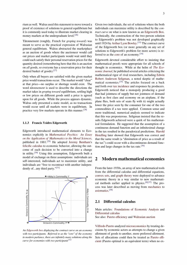
An Edgeworth box displaying the contract curve on an economywith two participants. Referred to as the “core” of the economyin modern parlance, there are infinitely many solutions along thecurve for economies with two participants[32]

Given two individuals, the set of solutions where the bothindividuals can maximize utility is described by the con-tract curve on what is now known as an Edgeworth Box.Technically, the construction of the two-person solutionto Edgeworth’s problem was not developed graphicallyuntil 1924 by Arthur Lyon Bowley.[33] The contract curveof the Edgeworth box (or more generally on any set ofsolutions to Edgeworth’s problem for more actors) is re-ferred to as the core of an economy.[34]

Edgeworth devoted considerable effort to insisting thatmathematical proofs were appropriate for all schools ofthought in economics. While at the helm of The Eco-nomic Journal, he published several articles criticizing themathematical rigor of rival researchers, including EdwinRobert Anderson Seligman, a noted skeptic of mathe-matical economics.[35] The articles focused on a backand forth over tax incidence and responses by producers.Edgeworth noticed that a monopoly producing a goodthat had jointness of supply but not jointness of demand(such as first class and economy on an airplane, if theplane flies, both sets of seats fly with it) might actuallylower the price seen by the consumer for one of the twocommodities if a tax were applied. Common sense andmore traditional, numerical analysis seemed to indicatethat this was preposterous. Seligman insisted that the re-sults Edgeworth achieved were a quirk of his mathemat-ical formulation. He suggested that the assumption of acontinuous demand function and an infinitesimal changein the tax resulted in the paradoxical predictions. HaroldHotelling later showed that Edgeworth was correct andthat the same result (a “diminution of price as a result ofthe tax”) could occur with a discontinuous demand func-tion and large changes in the tax rate.[36]

2 Modernmathematical economics

From the later-1930s, an array of newmathematical toolsfrom the differential calculus and differential equations,convex sets, and graph theory were deployed to advanceeconomic theory in a way similar to new mathemati-cal methods earlier applied to physics.[8][37] The pro-cess was later described as moving from mechanics toaxiomatics.[38]

2.1 Differential calculus

Main articles: Foundations of Economic Analysis andDifferential calculusSee also: Pareto efficiency and Walrasian auction

Vilfredo Pareto analyzed microeconomics by treating de-cisions by economic actors as attempts to change a givenallotment of goods to another, more preferred allotment.Sets of allocations could then be treated as Pareto effi-cient (Pareto optimal is an equivalent term) when no ex-

4 2 MODERN MATHEMATICAL ECONOMICS

changes could occur between actors that could make atleast one individual better off without making any otherindividual worse off.[39] Pareto’s proof is commonly con-flated with Walrassian equilibrium or informally ascribedto Adam Smith's Invisible hand hypothesis.[40] Rather,Pareto’s statement was the first formal assertion of whatwould be known as the first fundamental theorem of wel-fare economics.[41] These models lacked the inequalitiesof the next generation of mathematical economics.In the landmark treatise Foundations of EconomicAnalysis (1947), Paul Samuelson identified a commonparadigm and mathematical structure across multiplefields in the subject, building on previous work by AlfredMarshall. Foundations took mathematical concepts fromphysics and applied them to economic problems. Thisbroad view (for example, comparing Le Chatelier’s prin-ciple to tâtonnement) drives the fundamental premise ofmathematical economics: systems of economic actorsmay be modeled and their behavior described much likeany other system. This extension followed on the workof the marginalists in the previous century and extendedit significantly. Samuelson approached the problems ofapplying individual utility maximization over aggregategroups with comparative statics, which compares two dif-ferent equilibrium states after an exogenous change in avariable. This and other methods in the book providedthe foundation for mathematical economics in the 20thcentury.[7][42]

2.2 Linear models

See also: Linear algebra, Linear programming, andPerron–Frobenius theorem

Restricted models of general equilibrium were formu-lated by John von Neumann in 1937.[43] Unlike ear-lier versions, the models of von Neumann had inequal-ity constraints. For his model of an expanding econ-omy, von Neumann proved the existence and uniquenessof an equilibrium using his generalization of Brouwer’sfixed point theorem. Von Neumann’s model of an ex-panding economy considered the matrix pencil A - λ Bwith nonnegative matricesA and B; von Neumann soughtprobability vectors p and q and a positive number λ thatwould solve the complementarity equation

pT (A - λ B) q = 0,

along with two inequality systems expressing economicefficiency. In this model, the (transposed) probabilityvector p represents the prices of the goods while the prob-ability vector q represents the “intensity” at which theproduction process would run. The unique solution λ rep-resents the rate of growth of the economy, which equalsthe interest rate. Proving the existence of a positivegrowth rate and proving that the growth rate equals the

interest rate were remarkable achievements, even for vonNeumann.[44][45][46] Von Neumann’s results have beenviewed as a special case of linear programming, wherevon Neumann’s model uses only nonnegative matrices.[47]The study of von Neumann’s model of an expandingeconomy continues to interest mathematical economistswith interests in computational economics.[48][49][50]

2.2.1 Input-output economics

Main article: Input-output model

In 1936, the Russian–born economist Wassily Leontiefbuilt his model of input-output analysis from the 'materialbalance' tables constructed by Soviet economists, whichthemselves followed earlier work by the physiocrats.With his model, which described a system of productionand demand processes, Leontief described how changesin demand in one economic sector would influence pro-duction in another.[51] In practice, Leontief estimated thecoefficients of his simple models, to address econom-ically interesting questions. In production economics,“Leontief technologies” produce outputs using constantproportions of inputs, regardless of the price of inputs,reducing the value of Leontief models for understand-ing economies but allowing their parameters to be esti-mated relatively easily. In contrast, the von Neumannmodel of an expanding economy allows for choice oftechniques, but the coefficients must be estimated foreach technology.[52][53]

2.3 Mathematical optimization

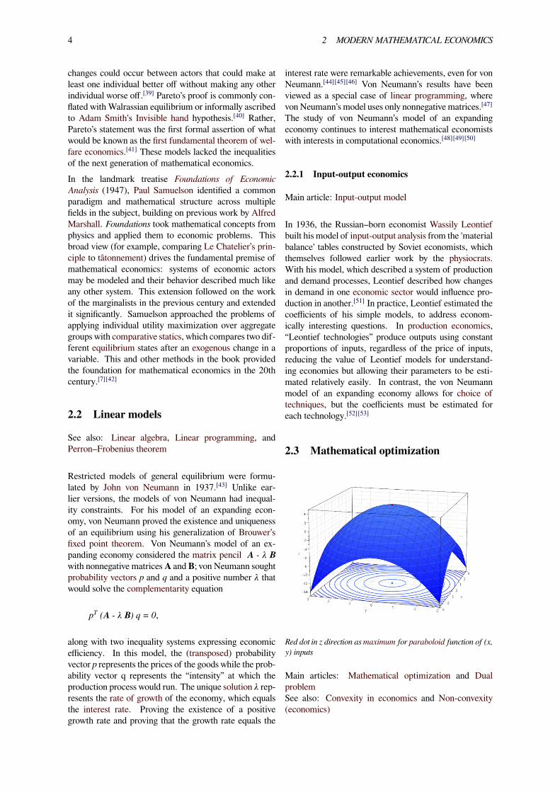
Red dot in z direction as maximum for paraboloid function of (x,y) inputs

Main articles: Mathematical optimization and DualproblemSee also: Convexity in economics and Non-convexity(economics)

2.3 Mathematical optimization 5

In mathematics, mathematical optimization (or optimiza-tion or mathematical programming) refers to the se-lection of a best element from some set of availablealternatives.[54] In the simplest case, an optimizationproblem involves maximizing or minimizing a real func-tion by selecting input values of the function and comput-ing the corresponding values of the function. The solutionprocess includes satisfying general necessary and suffi-cient conditions for optimality. For optimization prob-lems, specialized notation may be used as to the func-tion and its input(s). More generally, optimization in-cludes finding the best available element of some functiongiven a defined domain and may use a variety of differentcomputational optimization techniques.[55]

Economics is closely enough linked to optimization byagents in an economy that an influential definition relat-edly describes economics qua science as the “study of hu-man behavior as a relationship between ends and scarcemeans” with alternative uses.[56] Optimization problemsrun through modern economics, many with explicit eco-nomic or technical constraints. In microeconomics, theutility maximization problem and its dual problem, theexpenditure minimization problem for a given level ofutility, are economic optimization problems.[57] Theoryposits that consumers maximize their utility, subject totheir budget constraints and that firms maximize theirprofits, subject to their production functions, input costs,and market demand.[58]

Economic equilibrium is studied in optimization theoryas a key ingredient of economic theorems that in princi-ple could be tested against empirical data.[7][59] Newer de-velopments have occurred in dynamic programming andmodeling optimization with risk and uncertainty, includ-ing applications to portfolio theory, the economics of in-formation, and search theory.[58]

Optimality properties for an entire market system maybe stated in mathematical terms, as in formulation of thetwo fundamental theorems of welfare economics[60] andin the Arrow–Debreu model of general equilibrium (alsodiscussed below).[61] More concretely, many problemsare amenable to analytical (formulaic) solution. Manyothers may be sufficiently complex to require numericalmethods of solution, aided by software.[55] Still others arecomplex but tractable enough to allow computable meth-ods of solution, in particular computable general equilib-rium models for the entire economy.[62]

Linear and nonlinear programming have profoundly af-fected microeconomics, which had earlier consideredonly equality constraints.[63] Many of the mathematicaleconomists who received Nobel Prizes in Economics hadconducted notable research using linear programming:Leonid Kantorovich, Leonid Hurwicz, Tjalling Koop-mans, Kenneth J. Arrow, and Robert Dorfman, PaulSamuelson, and Robert Solow.[64] Both Kantorovich andKoopmans acknowledged that George B. Dantzig de-served to share their Nobel Prize for linear programming.

Economists who conducted research in nonlinear pro-gramming also have won the Nobel prize, notably RagnarFrisch in addition to Kantorovich, Hurwicz, Koopmans,Arrow, and Samuelson.

2.3.1 Linear optimization

Main articles: Linear programming and Simplex algo-rithm

Linear programming was developed to aid the allocationof resources in firms and in industries during the 1930s inRussia and during the 1940s in the United States. Duringthe Berlin airlift (1948), linear programming was usedto plan the shipment of supplies to prevent Berlin fromstarving after the Soviet blockade.[65][66]

2.3.2 Nonlinear programming

See also: Nonlinear programming, Lagrangian multi-plier, Karush–Kuhn–Tucker conditions, and Shadowprice

Extensions to nonlinear optimization with inequality con-straints were achieved in 1951 by Albert W. Tucker andHarold Kuhn, who considered the nonlinear optimizationproblem:

Minimize f ( x ) subject to g i( x ) ≤ 0 and hj( x ) = 0 where

f (.) is the function to be minimized

g i(.) ( j = 1, ...,m ) are the functions of theminequality constraints

h (.) ( j = 1, ..., l ) are the functions of the lequality constraints.

In allowing inequality constraints, the Kuhn–Tucker ap-proach generalized the classic method of Lagrange mul-tipliers, which (until then) had allowed only equalityconstraints.[67] The Kuhn–Tucker approach inspired fur-ther research on Lagrangian duality, including the treat-ment of inequality constraints.[68][69] The duality the-ory of nonlinear programming is particularly satisfactorywhen applied to convex minimization problems, whichenjoy the convex-analytic duality theory of Fenchel andRockafellar; this convex duality is particularly strongfor polyhedral convex functions, such as those arisingin linear programming. Lagrangian duality and con-vex analysis are used daily in operations research, in thescheduling of power plants, the planning of productionschedules for factories, and the routing of airlines (routes,flights, planes, crews).[69]

6 2 MODERN MATHEMATICAL ECONOMICS

2.3.3 Variational calculus and optimal control

See also: Calculus of variations, Optimal control, andDynamic programming

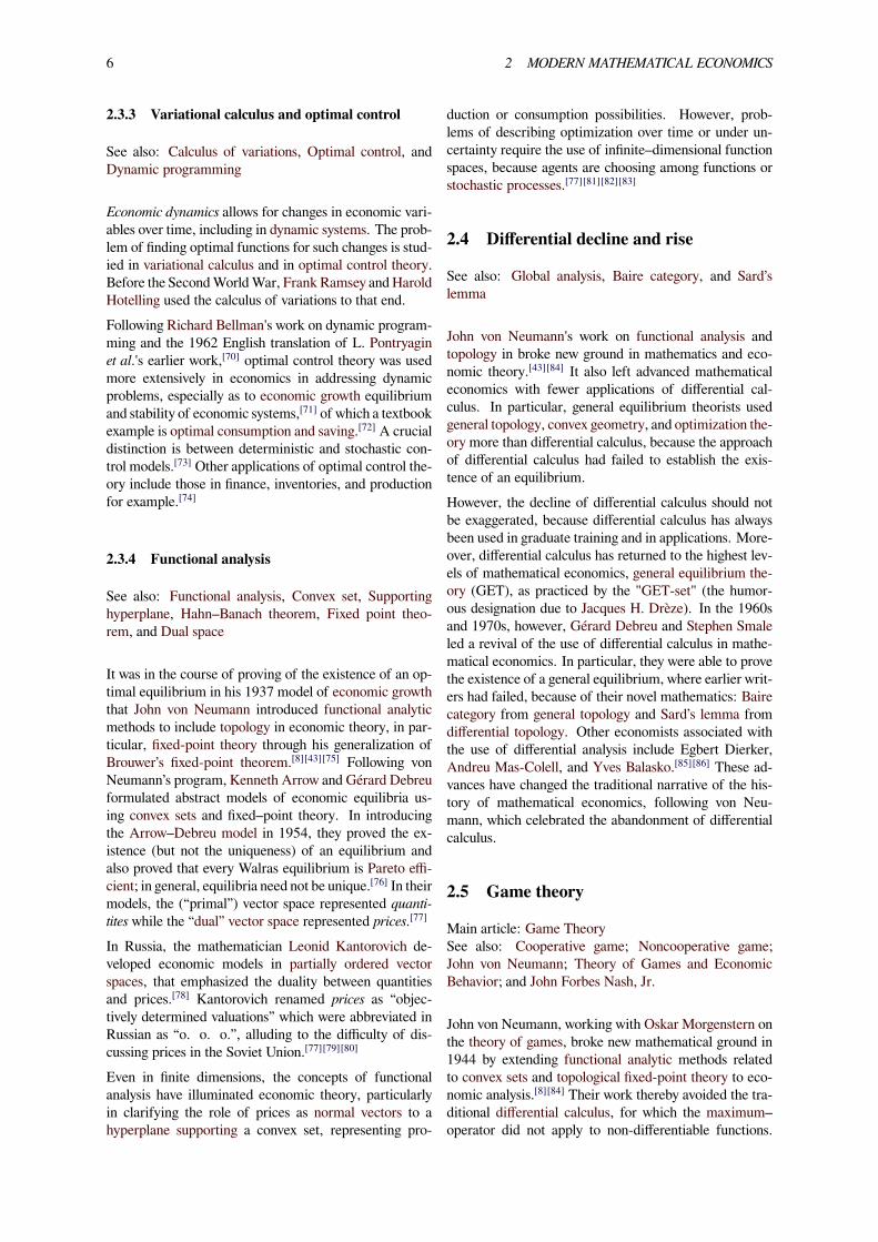
Economic dynamics allows for changes in economic vari-ables over time, including in dynamic systems. The prob-lem of finding optimal functions for such changes is stud-ied in variational calculus and in optimal control theory.Before the SecondWorldWar, Frank Ramsey and HaroldHotelling used the calculus of variations to that end.Following Richard Bellman's work on dynamic program-ming and the 1962 English translation of L. Pontryaginet al.'s earlier work,[70] optimal control theory was usedmore extensively in economics in addressing dynamicproblems, especially as to economic growth equilibriumand stability of economic systems,[71] of which a textbookexample is optimal consumption and saving.[72] A crucialdistinction is between deterministic and stochastic con-trol models.[73] Other applications of optimal control the-ory include those in finance, inventories, and productionfor example.[74]

2.3.4 Functional analysis

See also: Functional analysis, Convex set, Supportinghyperplane, Hahn–Banach theorem, Fixed point theo-rem, and Dual space

It was in the course of proving of the existence of an op-timal equilibrium in his 1937 model of economic growththat John von Neumann introduced functional analyticmethods to include topology in economic theory, in par-ticular, fixed-point theory through his generalization ofBrouwer’s fixed-point theorem.[8][43][75] Following vonNeumann’s program, Kenneth Arrow and Gérard Debreuformulated abstract models of economic equilibria us-ing convex sets and fixed–point theory. In introducingthe Arrow–Debreu model in 1954, they proved the ex-istence (but not the uniqueness) of an equilibrium andalso proved that every Walras equilibrium is Pareto effi-cient; in general, equilibria need not be unique.[76] In theirmodels, the (“primal”) vector space represented quanti-tites while the “dual” vector space represented prices.[77]

In Russia, the mathematician Leonid Kantorovich de-veloped economic models in partially ordered vectorspaces, that emphasized the duality between quantitiesand prices.[78] Kantorovich renamed prices as “objec-tively determined valuations” which were abbreviated inRussian as “o. o. o.”, alluding to the difficulty of dis-cussing prices in the Soviet Union.[77][79][80]

Even in finite dimensions, the concepts of functionalanalysis have illuminated economic theory, particularlyin clarifying the role of prices as normal vectors to ahyperplane supporting a convex set, representing pro-

duction or consumption possibilities. However, prob-lems of describing optimization over time or under un-certainty require the use of infinite–dimensional functionspaces, because agents are choosing among functions orstochastic processes.[77][81][82][83]

2.4 Differential decline and rise

See also: Global analysis, Baire category, and Sard’slemma

John von Neumann's work on functional analysis andtopology in broke new ground in mathematics and eco-nomic theory.[43][84] It also left advanced mathematicaleconomics with fewer applications of differential cal-culus. In particular, general equilibrium theorists usedgeneral topology, convex geometry, and optimization the-ory more than differential calculus, because the approachof differential calculus had failed to establish the exis-tence of an equilibrium.However, the decline of differential calculus should notbe exaggerated, because differential calculus has alwaysbeen used in graduate training and in applications. More-over, differential calculus has returned to the highest lev-els of mathematical economics, general equilibrium the-ory (GET), as practiced by the "GET-set" (the humor-ous designation due to Jacques H. Drèze). In the 1960sand 1970s, however, Gérard Debreu and Stephen Smaleled a revival of the use of differential calculus in mathe-matical economics. In particular, they were able to provethe existence of a general equilibrium, where earlier writ-ers had failed, because of their novel mathematics: Bairecategory from general topology and Sard’s lemma fromdifferential topology. Other economists associated withthe use of differential analysis include Egbert Dierker,Andreu Mas-Colell, and Yves Balasko.[85][86] These ad-vances have changed the traditional narrative of the his-tory of mathematical economics, following von Neu-mann, which celebrated the abandonment of differentialcalculus.

2.5 Game theory

Main article: Game TheorySee also: Cooperative game; Noncooperative game;John von Neumann; Theory of Games and EconomicBehavior; and John Forbes Nash, Jr.

John von Neumann, working with Oskar Morgenstern onthe theory of games, broke new mathematical ground in1944 by extending functional analytic methods relatedto convex sets and topological fixed-point theory to eco-nomic analysis.[8][84] Their work thereby avoided the tra-ditional differential calculus, for which the maximum–operator did not apply to non-differentiable functions.

7

Continuing von Neumann’s work in cooperative gametheory, game theorists Lloyd S. Shapley, Martin Shu-bik, HervéMoulin, NimrodMegiddo, Bezalel Peleg influ-enced economic research in politics and economics. Forexample, research on the fair prices in cooperative gamesand fair values for voting games led to changed rules forvoting in legislatures and for accounting for the costs inpublic–works projects. For example, cooperative gametheory was used in designing the water distribution sys-tem of Southern Sweden and for setting rates for dedi-cated telephone lines in the USA.Earlier neoclassical theory had bounded only the rangeof bargaining outcomes and in special cases, for ex-ample bilateral monopoly or along the contract curveof the Edgeworth box.[87] Von Neumann and Mor-genstern’s results were similarly weak. Followingvon Neumann’s program, however, John Nash usedfixed–point theory to prove conditions under which thebargaining problem and noncooperative games can gen-erate a unique equilibrium solution.[88] Noncoopera-tive game theory has been adopted as a fundamentalaspect of experimental economics,[89] behavioral eco-nomics,[90] information economics,[91] industrial organi-zation,[92] and political economy.[93] It has also given riseto the subject of mechanism design (sometimes called re-verse game theory), which has private and public-policyapplications as to ways of improving economic efficiencythrough incentives for information sharing.[94]

In 1994, Nash, John Harsanyi, and Reinhard Selten re-ceived the Nobel Memorial Prize in Economic Sciencestheir work on non–cooperative games. Harsanyi and Sel-ten were awarded for their work on repeated games. Laterwork extended their results to computational methods ofmodeling.[95]

2.6 Agent-based computational economics

Main article: Agent-based computational economics

Agent-based computational economics (ACE) as anamed field is relatively recent, dating from about the1990s as to published work. It studies economic pro-cesses, including whole economies, as dynamic systemsof interacting agents over time. As such, it falls inthe paradigm of complex adaptive systems.[96] In corre-sponding agent-based models, agents are not real peo-ple but “computational objects modeled as interacting ac-cording to rules” ... “whose micro-level interactions cre-ate emergent patterns” in space and time.[97] The rulesare formulated to predict behavior and social interactionsbased on incentives and information. The theoretical as-sumption of mathematical optimization by agents marketsis replaced by the less restrictive postulate of agents withbounded rationality adapting to market forces.[98]

ACE models apply numerical methods of analysis tocomputer-based simulations of complex dynamic prob-

lems for which more conventional methods, such as theo-rem formulation, may not find ready use.[99] Starting fromspecified initial conditions, the computational economicsystem is modeled as evolving over time as its constituentagents repeatedly interact with each other. In theserespects, ACE has been characterized as a bottom-upculture-dish approach to the study of the economy.[100]In contrast to other standard modeling methods, ACEevents are driven solely by initial conditions, whetheror not equilibria exist or are computationally tractable.ACE modeling, however, includes agent adaptation, au-tonomy, and learning.[101] It has a similarity to, and over-lap with, game theory as an agent-based method formodeling social interactions.[95] Other dimensions of theapproach include such standard economic subjects ascompetition and collaboration,[102] market structure andindustrial organization,[103] transaction costs,[104] welfareeconomics[105] and mechanism design,[94] informationand uncertainty,[106] and macroeconomics.[107][108]

The method is said to benefit from continuing improve-ments in modeling techniques of computer science andincreased computer capabilities. Issues include thosecommon to experimental economics in general[109] and bycomparison[110] and to development of a common frame-work for empirical validation and resolving open ques-tions in agent-based modeling.[111] The ultimate scientificobjective of the method has been described as “test[ing]theoretical findings against real-world data in ways thatpermit empirically supported theories to cumulate overtime, with each researcher’s work building appropriatelyon the work that has gone before.”[112]

3 Mathematicization of economics

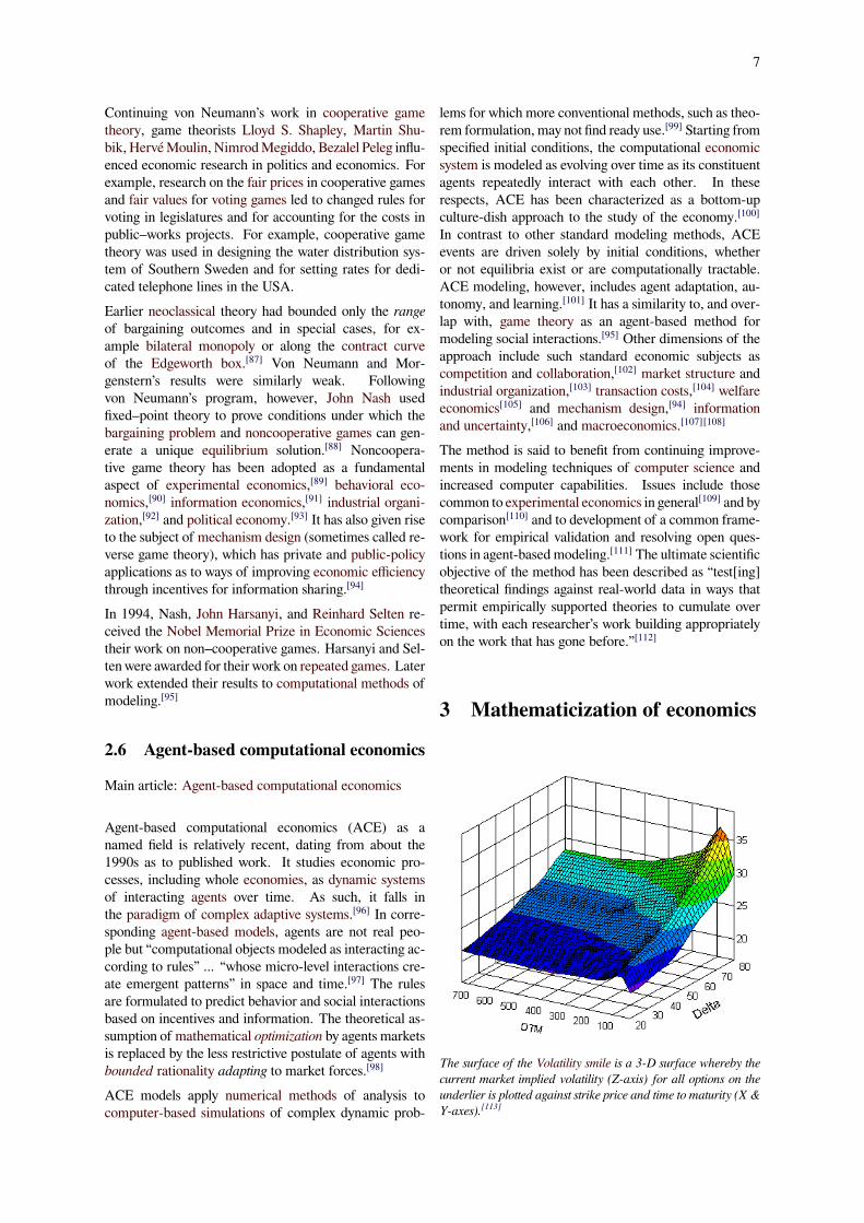
The surface of the Volatility smile is a 3-D surface whereby thecurrent market implied volatility (Z-axis) for all options on theunderlier is plotted against strike price and time to maturity (X &Y-axes).[113]

8 5 APPLICATION

Over the course of the 20th century, articles in “corejournals”[114] in economics have been almost exclusivelywritten by economists in academia. As a result, much ofthe material transmitted in those journals relates to eco-nomic theory, and “economic theory itself has been con-tinuously more abstract and mathematical.”[115] A sub-jective assessment of mathematical techniques[116] em-ployed in these core journals showed a decrease in articlesthat use neither geometric representations nor mathemat-ical notation from 95% in 1892 to 5.3% in 1990.[117] A2007 survey of ten of the top economic journals finds thatonly 5.8% of the articles published in 2003 and 2004 bothlacked statistical analysis of data and lacked displayedmathematical expressions that were indexed with num-bers at the margin of the page.[118]

4 Econometrics

Main article: Econometrics

Between the world wars, advances in mathematical statis-tics and a cadre of mathematically trained economists ledto econometrics, which was the name proposed for thediscipline of advancing economics by using mathematicsand statistics. Within economics, “econometrics” has of-ten been used for statistical methods in economics, ratherthan mathematical economics. Statistical econometricsfeatures the application of linear regression and time se-ries analysis to economic data.Ragnar Frisch coined the word “econometrics” andhelped to found both the Econometric Society in 1930and the journal Econometrica in 1933.[119][120] A studentof Frisch’s, Trygve Haavelmo published The ProbabilityApproach in Econometrics in 1944, where he asserted thatprecise statistical analysis could be used as a tool to val-idate mathematical theories about economic actors withdata from complex sources.[121] This linking of statisticalanalysis of systems to economic theory was also promul-gated by the Cowles Commission (now the Cowles Foun-dation) throughout the 1930s and 1940s.[122]

The roots of modern econometrics can be traced to theAmerican economist Henry L. Moore. Moore studiedagricultural productivity and attempted to fit changingvalues of productivity for plots of corn and other crops toa curve using different values of elasticity. Moore madeseveral errors in his work, some from his choice ofmodelsand some from limitations in his use of mathematics. Theaccuracy of Moore’s models also was limited by the poordata for national accounts in the United States at the time.While his first models of production were static, in 1925he published a dynamic “moving equilibrium” model de-signed to explain business cycles—this periodic variationfrom overcorrection in supply and demand curves is nowknown as the cobweb model. A more formal derivationof this model was made later by Nicholas Kaldor, who is

largely credited for its exposition.[123]

5 Application

LM

IS1

IS2

i

YY1 Y2

i2

i1

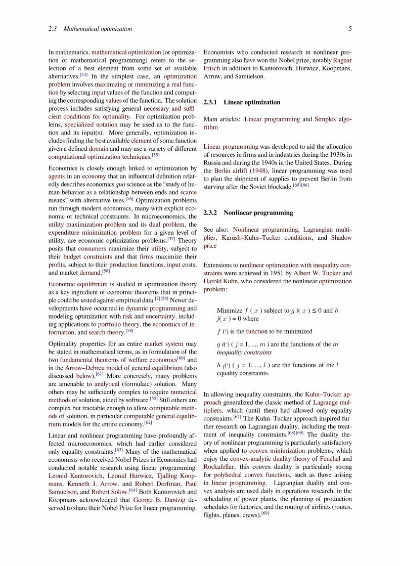
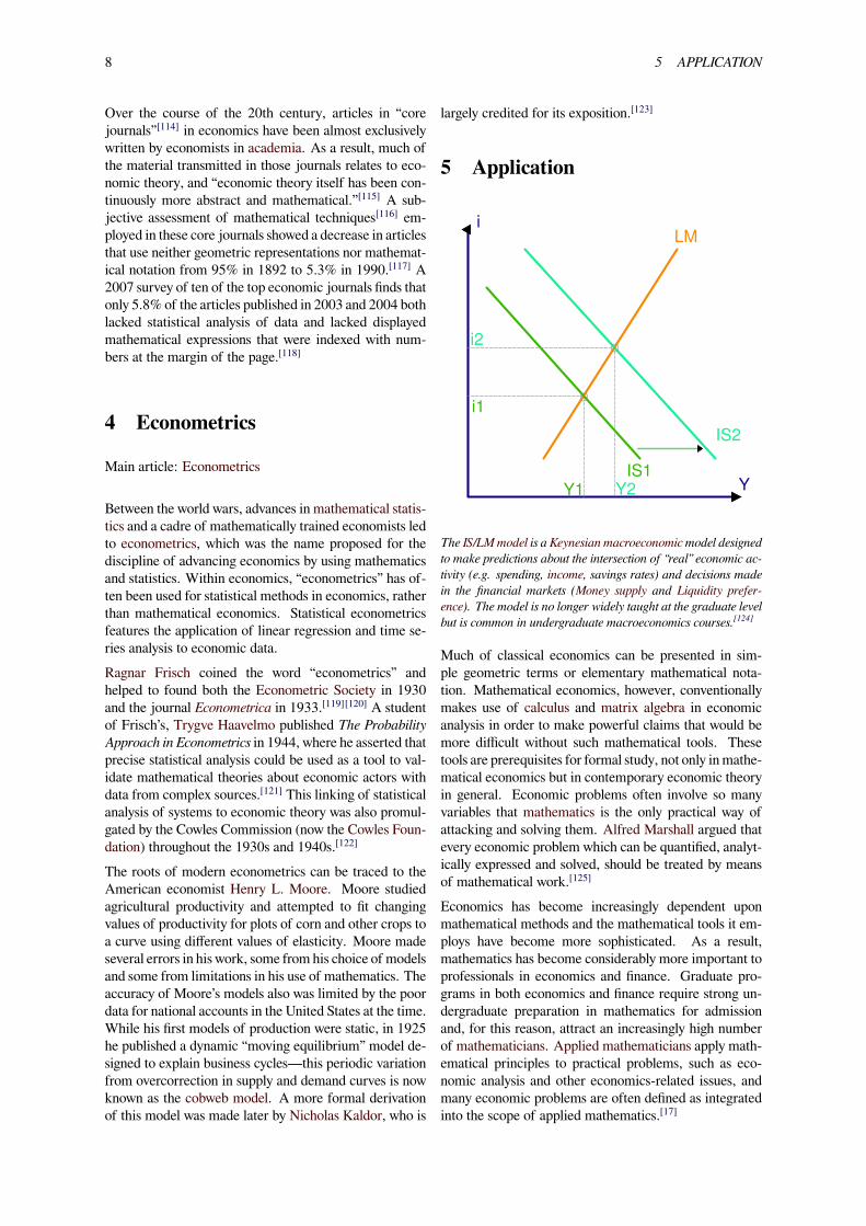
The IS/LMmodel is a Keynesian macroeconomic model designedto make predictions about the intersection of “real” economic ac-tivity (e.g. spending, income, savings rates) and decisions madein the financial markets (Money supply and Liquidity prefer-ence). The model is no longer widely taught at the graduate levelbut is common in undergraduate macroeconomics courses.[124]

Much of classical economics can be presented in sim-ple geometric terms or elementary mathematical nota-tion. Mathematical economics, however, conventionallymakes use of calculus and matrix algebra in economicanalysis in order to make powerful claims that would bemore difficult without such mathematical tools. Thesetools are prerequisites for formal study, not only inmathe-matical economics but in contemporary economic theoryin general. Economic problems often involve so manyvariables that mathematics is the only practical way ofattacking and solving them. Alfred Marshall argued thatevery economic problem which can be quantified, analyt-ically expressed and solved, should be treated by meansof mathematical work.[125]

Economics has become increasingly dependent uponmathematical methods and the mathematical tools it em-ploys have become more sophisticated. As a result,mathematics has become considerably more important toprofessionals in economics and finance. Graduate pro-grams in both economics and finance require strong un-dergraduate preparation in mathematics for admissionand, for this reason, attract an increasingly high numberof mathematicians. Applied mathematicians apply math-ematical principles to practical problems, such as eco-nomic analysis and other economics-related issues, andmany economic problems are often defined as integratedinto the scope of applied mathematics.[17]

9

This integration results from the formulation of economicproblems as stylized models with clear assumptions andfalsifiable predictions. This modeling may be informal orprosaic, as it was in Adam Smith's TheWealth of Nations,or it may be formal, rigorous and mathematical.Broadly speaking, formal economic models may be clas-sified as stochastic or deterministic and as discrete or con-tinuous. At a practical level, quantitative modeling is ap-plied to many areas of economics and several method-ologies have evolved more or less independently of eachother.[126]

• Stochastic models are formulated using stochasticprocesses. They model economically observablevalues over time. Most of econometrics is basedon statistics to formulate and test hypotheses aboutthese processes or estimate parameters for them.Between the World Wars, Herman Wold developeda representation of stationary stochastic processesin terms of autoregressive models and a deterministtrend. Wold and Jan Tinbergen applied time-seriesanalysis to economic data. Contemporary researchon time series statistics consider additional formula-tions of stationary processes, such as autoregressivemoving average models. More general models in-clude autoregressive conditional heteroskedasticity(ARCH) models and generalized ARCH (GARCH)models.

• Non-stochastic mathematical models may be purelyqualitative (for example, models involved in someaspect of social choice theory) or quantitative (in-volving rationalization of financial variables, forexample with hyperbolic coordinates, and/or spe-cific forms of functional relationships between vari-ables). In some cases economic predictions of amodel merely assert the direction of movement ofeconomic variables, and so the functional relation-ships are used only in a qualitative sense: for ex-ample, if the price of an item increases, then thedemand for that item will decrease. For such mod-els, economists often use two-dimensional graphsinstead of functions.

• Qualitative models are occasionally used. One ex-ample is qualitative scenario planning in which pos-sible future events are played out. Another exampleis non-numerical decision tree analysis. Qualitativemodels often suffer from lack of precision.

6 Classification

According to the Mathematics Subject Classification(MSC), mathematical economics falls into the Appliedmathematics/other classification of category 91:

Game theory, economics, social and behavioralsciences

with MSC2010 classifications for 'Game theory' at codes91Axx and for 'Mathematical economics’ at codes 91Bxx.The Handbook of Mathematical Economics series (Else-vier), currently 4 volumes, distinguishes between math-ematical methods in economics, v. 1, Part I, and ar-eas of economics in other volumes where mathematics isemployed.[127]

Another source with a similar distinction is The New Pal-grave: A Dictionary of Economics (1987, 4 vols., 1,300subject entries). In it, a “Subject Index” includes mathe-matical entries under 2 headings (vol. IV, pp. 982–3):

Mathematical Economics (24 listed, suchas “acyclicity”, "aggregation problem","comparative statics", "lexicographic or-derings", "linear models", "orderings", and"qualitative economics")Mathematical Methods (42 listed, such as"calculus of variations", "catastrophe the-ory", "combinatorics,” "computation of gen-eral equilibrium", "convexity", "convex pro-gramming", and “stochastic optimal control").

A widely used system in economics that includes mathe-matical methods on the subject is the JEL classificationcodes. It originated in the Journal of Economic Literaturefor classifying new books and articles. The relevant cat-egories are listed below (simplified below to omit “Mis-cellaneous” and “Other” JEL codes), as reproduced fromJEL classification codes#Mathematical and quantitativemethods JEL: C Subcategories. The New Palgrave Dic-tionary of Economics (2008, 2nd ed.) also uses the JELcodes to classify its entries. The corresponding footnotesbelow have links to abstracts of The New Palgrave Onlinefor each JEL category (10 or fewer per page, similar toGoogle searches).

JEL: C02 - Mathematical Methods (follow-ing JEL: C00 - General and JEL: C01 -Econometrics)

JEL: C6 - Mathematical Methods;Programming Models; Mathematical andSimulation Modeling [128]

JEL: C60 - GeneralJEL: C61 - Optimization tech-niques; Programming models;Dynamic analysis[129]JEL: C62 - Existence and stabilityconditions of equilibrium[130]

JEL: C63 - Computational tech-niques; Simulation modeling[131]JEL: C67 - Input–output modelsJEL: C68 - Computable GeneralEquilibrium models[132]

10 7 CRITICISMS AND DEFENCES

JEL: C7 - Game theory and Bargaining the-ory[133]

JEL: C70 - General[134]JEL: C71 - Cooperative games[135]JEL: C72 - Noncooperativegames[136]JEL: C73 - Stochastic and Dynamicgames; Evolutionary games; Re-peated Games[137]JEL: C78 - Bargaining theory;Matching theory[138]

7 Criticisms and defences

7.1 Adequacy of mathematics for qualita-tive and complicated economics

Friedrich Hayek contended that the use of formal tech-niques projects a scientific exactness that does not ap-propriately account for informational limitations faced byreal economic agents. [139]

In an interview, the economic historian Robert Heil-broner stated:[140]

I guess the scientific approach began topenetrate and soon dominate the profession inthe past twenty to thirty years. This came aboutin part because of the “invention” of mathe-matical analysis of various kinds and, indeed,considerable improvements in it. This is theage in which we have not only more data butmore sophisticated use of data. So there is astrong feeling that this is a data-laden scienceand a data-laden undertaking, which, by virtueof the sheer numerics, the sheer equations, andthe sheer look of a journal page, bears a cer-tain resemblance to science . . . That one cen-tral activity looks scientific. I understand that.I think that is genuine. It approaches being auniversal law. But resembling a science is dif-ferent from being a science.

Heilbroner stated that “some/much of economics is notnaturally quantitative and therefore does not lend itself tomathematical exposition.”[141]

7.2 Testing predictions of mathematicaleconomics

Philosopher Karl Popper discussed the scientific stand-ing of economics in the 1940s and 1950s. He arguedthat mathematical economics suffered from being tau-tological. In other words, insofar that economics be-came a mathematical theory, mathematical economics

ceased to rely on empirical refutation but rather relied onmathematical proofs and disproof.[142] According to Pop-per, falsifiable assumptions can be tested by experimentand observation while unfalsifiable assumptions can beexplored mathematically for their consequences and fortheir consistency with other assumptions.[143]

Sharing Popper’s concerns about assumptions in eco-nomics generally, and not just mathematical economics,Milton Friedman declared that “all assumptions are un-realistic”. Friedman proposed judging economic modelsby their predictive performance rather than by the matchbetween their assumptions and reality.[144]

7.3 Mathematical economics as a form ofpure mathematics

See also: Pure mathematics, Applied mathematics, andEngineering

Consideringmathematical economics, J.M. Keynes wrotein The General Theory:[145]

It is a great fault of symbolic pseudo-mathematical methods of formalising a systemof economic analysis ... that they expressly as-sume strict independence between the factorsinvolved and lose their cogency and authorityif this hypothesis is disallowed; whereas, in or-dinary discourse, where we are not blindly ma-nipulating and know all the time what we aredoing and what the words mean, we can keep‘at the back of our heads’ the necessary reservesand qualifications and the adjustments whichwe shall have to make later on, in a way inwhich we cannot keep complicated partial dif-ferentials ‘at the back’ of several pages of alge-bra which assume they all vanish. Too large aproportion of recent ‘mathematical’ economicsare merely concoctions, as imprecise as the ini-tial assumptions they rest on, which allow theauthor to lose sight of the complexities and in-terdependencies of the real world in a maze ofpretentious and unhelpful symbols.

7.4 Defense of mathematical economics

In response to these criticisms, Paul Samuelson ar-gued that mathematics is a language, repeating a the-sis of Josiah Willard Gibbs. In economics, the lan-guage of mathematics is sometimes necessary for rep-resenting substantive problems. Moreover, mathe-matical economics has led to conceptual advances ineconomics.[146] In particular, Samuelson gave the exam-ple of microeconomics, writing that “few people are inge-nious enough to grasp [its] more complex parts... without

11

resorting to the language of mathematics, while most or-dinary individuals can do so fairly easily with the aid ofmathematics.”[147]

Some economists state that mathematical economics de-serves support just like other forms of mathematics,particularly its neighbors in mathematical optimizationand mathematical statistics and increasingly in theoreticalcomputer science. Mathematical economics and othermathematical sciences have a history in which theoreti-cal advances have regularly contributed to the reform ofthe more applied branches of economics. In particular,following the program of John von Neumann, game the-ory now provides the foundations for describing muchof applied economics, from statistical decision theory(as “games against nature”) and econometrics to generalequilibrium theory and industrial organization. In thelast decade, with the rise of the internet, mathematicaleconomicists and optimization experts and computer sci-entists have worked on problems of pricing for on-lineservices --- their contributions using mathematics fromcooperative game theory, nondifferentiable optimization,and combinatorial games.Robert M. Solow concluded that mathematical eco-nomics was the core "infrastructure" of contemporaryeconomics:

Economics is no longer a fit conversationpiece for ladies and gentlemen. It has becomea technical subject. Like any technical sub-ject it attracts some people who are more inter-ested in the technique than the subject. That istoo bad, but it may be inevitable. In any case,do not kid yourself: the technical core of eco-nomics is indispensable infrastructure for thepolitical economy. That is why, if you con-sult [a reference in contemporary economics]looking for enlightenment about the world to-day, you will be led to technical economics, orhistory, or nothing at all.[148]

8 Mathematical economists

Prominent mathematical economists include, but are notlimited to, the following (by century of birth).

8.1 19th century

8.2 20th century

9 See also/Related fields

• Econophysics

• Mathematical finance

10 Notes[1] Elaborated at the JEL classification codes, Mathematical

and quantitative methods JEL: C Subcategories.

[2] Chiang, Alpha C.; Kevin Wainwright (2005). Fundamen-tal Methods of Mathematical Economics. McGraw-Hill Ir-win. pp. 3–4. ISBN 0-07-010910-9. TOC.

[3] Debreu, Gérard ([1987] 2008). “mathematical eco-nomics”, section II, The New Palgrave Dictionary of Eco-nomics, 2nd Edition. Abstract. Republished with re-visions from 1986, “Theoretic Models: MathematicalForm and Economic Content”, Econometrica, 54(6), pp.1259−1270.

[4] Varian, Hal (1997). “What Use Is Economic Theory?" inA. D'Autume and J. Cartelier, ed., Is Economics Becom-ing a Hard Science?, Edward Elgar. Pre-publication PDF.Retrieved 2008-04-01.

[5] • As in Handbook of Mathematical Economics, 1st-pagechapter links:Arrow, Kenneth J., and Michael D. Intriligator, ed.,(1981), v. 1_____ (1982). v. 2_____ (1986). v. 3Hildenbrand, Werner, and Hugo Sonnenschein, ed.(1991). v. 4.• Debreu, Gérard (1983). Mathematical Economics:Twenty Papers of Gérard Debreu, Contents.• Glaister, Stephen (1984). Mathematical Methods forEconomists, 3rd ed., Blackwell. Contents.• Takayama, Akira (1985). Mathematical Economics, 2nded. Cambridge. Description and Contents.• Michael Carter (2001). Foundations of MathematicalEconomics, MIT Press. Description and Contents.

[6] Chiang, Alpha C. (1992). Elements of Dynamic Optimiza-tion, Waveland. TOC & Amazon.com link to inside, firstpp.

[7] Samuelson, Paul ((1947) [1983]). Foundations of Eco-nomic Analysis. Harvard University Press. ISBN 0-674-31301-1. Check date values in: |date= (help)

[8] • Debreu, Gérard ([1987] 2008). “mathematical eco-nomics”, The New Palgrave Dictionary of Economics, 2ndEdition. Abstract. Republished with revisions from 1986,“Theoretic Models: Mathematical Form and EconomicContent”, Econometrica, 54(6), pp. 1259−1270.• von Neumann, John, and Oskar Morgenstern (1944).Theory of Games and Economic Behavior. Princeton Uni-versity Press.

[9] Schumpeter, J.A. (1954). Elizabeth B. Schumpeter, ed.History of Economic Analysis. New York: Oxford Uni-versity Press. pp. 209–212. ISBN 978-0-04-330086-2.OCLC 13498913.

[10] Schumpeter (1954) p. 212-215

[11] Schnieder, Erich (1934). “Johann Heinrich von Thü-nen”. Econometrica. The Econometric Society. 2 (1):1–12. doi:10.2307/1907947. ISSN 0012-9682. JSTOR1907947. OCLC 35705710.

12 10 NOTES

[12] Schumpeter (1954) p. 465-468

[13] Philip Mirowski, 1991. “The When, the How and theWhy of Mathematical Expression in the History of Eco-nomics Analysis”, Journal of Economic Perspectives, 5(1)pp. 145-157.

[14] Weintraub, E. Roy (2008). “mathematics and eco-nomics”, The New Palgrave Dictionary of Economics, 2ndEdition. Abstract.

[15] Jevons, W.S. (1866). “Brief Account of a General Math-ematical Theory of Political Economy”, Journal of theRoyal Statistical Society, XXIX (June) pp. 282-87. Readin Section F of the British Association, 1862. PDF.

[16] Jevons, W. Stanley (1871). The Principles of PoliticalEconomy, pp. 4, 25.

[17] Sheila C., Dow (1999-05-21). “The Use of Mathematicsin Economics”. ESRC Public Understanding ofMathemat-ics Seminar. Birmingham: Economic and Social ResearchCouncil. Retrieved 2008-07-06.

[18] While the concept of cardinality has fallen out of favor inneoclassical economics, the differences between cardinalutility and ordinal utility are minor for most applications.

[19] Nicola, PierCarlo (2000). Mainstream MathermaticalEconomics in the 20th Century. Springer. p. 4. ISBN978-3-540-67084-1. Retrieved 2008-08-21.

[20] Augustin Cournot (1838, tr. 1897) Researches into theMathematical Principles of Wealth. Links to descriptionand chapters.

[21] Hotelling, Harold (1990). “Stability in Competition”. InDarnell, Adrian C. The Collected Economics Articles ofHarold Hotelling. Springer. pp. 51, 52. ISBN 3-540-97011-8. OCLC 20217006. Retrieved 2008-08-21.

[22] “Antoine Augustin Cournot, 1801-1877”. The History ofEconomic Thought Website. The New School for SocialResearch. Retrieved 2008-08-21.

[23] Gibbons, Robert (1992). Game Theory for AppliedEconomists. Princeton, New Jersey: Princeton UniversityPress. pp. 14, 15. ISBN 0-691-00395-5.

[24] Nicola, p. 9-12

[25] Edgeworth, Francis Ysidro (September 5, 1889).“The Mathematical Theory of Political Economy:Review of Léon Walras, Éléments d'économie poli-tique pure” (PDF). Nature. 40 (1036): 434–436.doi:10.1038/040434a0. ISSN 0028-0836. Retrieved2008-08-21.

[26] Nicholson, Walter; Snyder, Christopher, p. 350-353.

[27] Dixon, Robert. “Walras Law and Macroeconomics”.Walras Law Guide. Department of Economics, Univer-sity of Melbourne. Archived from the original on April17, 2008. Retrieved 2008-09-28.

[28] Dixon, Robert. “A Formal Proof of Walras Law”. Wal-ras Law Guide. Department of Economics, University ofMelbourne. Archived from the original onApril 30, 2008.Retrieved 2008-09-28.

[29] Rima, Ingrid H. (1977). “Neoclassicism and Dissent1890-1930”. In Weintraub, Sidney. Modern EconomicThought. University of Pennsylvania Press. pp. 10, 11.ISBN 0-8122-7712-0.

[30] Heilbroner, Robert L. (1953 [1999]). The WorldlyPhilosophers (Seventh ed.). New York: Simon and Schus-ter. pp. 172–175, 313. ISBN 978-0-684-86214-9.Check date values in: |date= (help)

[31] Edgeworth, Francis Ysidro (1881 [1961]). MathematicalPsychics. London: Kegan Paul [A. M. Kelley]. pp. 15–19. Check date values in: |date= (help)

[32] Nicola, p. 14, 15, 258-261

[33] Bowley, Arthur Lyon (1924 [1960]). The Mathemati-cal Groundwork of Economics: an Introductory Treatise.Oxford: Clarendon Press [Kelly]. Check date values in:|date= (help)

[34] Gillies, D. B. (1969). “Solutions to general non-zero-sumgames”. In Tucker, A.W.; Luce, R. D.Contributions to theTheory of Games. Annals of Mathematics. 40. Prince-ton, New Jersey: Princeton University Press. pp. 47–85.ISBN 978-0-691-07937-0.

[35] Moss, Lawrence S. (2003). “The Seligman-EdgeworthDebate about the Analysis of Tax Incidence: The Adventof Mathematical Economics, 1892–1910”. History of Po-litical Economy. Duke University Press. 35 (2): 207, 212,219, 234–237. doi:10.1215/00182702-35-2-205. ISSN0018-2702.

[36] Hotelling, Harold (1990). “Note on Edgeworth’s Taxa-tion Phenomenon and Professor Garver’s Additional Con-dition on Demand Functions”. In Darnell, Adrian C.The Collected Economics Articles of Harold Hotelling.Springer. pp. 94–122. ISBN 3-540-97011-8. OCLC20217006. Retrieved 2008-08-26.

[37] Herstein, I.N. (October 1953). “Some MathematicalMethods and Techniques in Economics”. Quarterly of Ap-plied Mathematics. American Mathematical Society. 11(3): 249, 252, 260. ISSN 1552-4485. [Pp. 249-62.

[38] • Weintraub, E. Roy (2008). “mathematics and eco-nomics”, The New Palgrave Dictionary of Economics, 2ndEdition. Abstract.• _____ (2002). How Economics Became a MathematicalScience. Duke University Press. Description and preview.

[39] Nicholson, Walter; Snyder, Christopher (2007). “GeneralEquilibrium and Welfare”. Intermediate Microeconomicsand Its Applications (10th ed.). Thompson. pp. 364, 365.ISBN 0-324-31968-1.

[40] Jolink, Albert (2006). “WhatWentWrong withWalras?".In Backhaus, Juergen G.; Maks, J.A. Hans. From Walrasto Pareto. The European Heritage in Economics and theSocial Sciences. IV. Springer. doi:10.1007/978-0-387-33757-9_6. ISBN 978-0-387-33756-2.• Blaug, Mark (2007). “The Fundamental Theorems ofModern Welfare Economics, Historically Contemplated”.History of Political Economy. Duke University Press. 39(2): 186–188. doi:10.1215/00182702-2007-001. ISSN0018-2702.

13

[41] Blaug (2007), p. 185, 187

[42] Metzler, Lloyd (1948). “Review of Foundations of Eco-nomic Analysis". American Economic Review. The Amer-ican Economic Review, Vol. 38, No. 5. 38 (5): 905–910.ISSN 0002-8282. JSTOR 1811704.

[43] Neumann, J. von (1937). "Über ein ökonomisches Gle-ichungssystem und ein Verallgemeinerung des Brouwer-schen Fixpunktsatzes”, Ergebnisse eines MathematischenKolloquiums, 8, pp. 73-83, translated and published in1945-46, as “A Model of General Equilibrium”, Reviewof Economic Studies, 13, pp. 1–9.

[44] For this problem to have a unique solution, it suffices thatthe nonnegative matrices A and B satisfy an irreducibilitycondition, generalizing that of the Perron–Frobenius the-orem of nonnegative matrices, which considers the (sim-plified) eigenvalue problem

A - λ I q = 0,

where the nonnegative matrixAmust be square and wherethe diagonal matrix I is the identity matrix. Von Neu-mann’s irreducibility condition was called the “whalesand wranglers" hypothesis by David Champernowne, whoprovided a verbal and economic commentary on the En-glish translation of von Neumann’s article. Von Neu-mann’s hypothesis implied that every economic processused a positive amount of every economic good. Weaker“irreducibility” conditions were given by David Gale andby John Kemeny, Oskar Morgenstern, and Gerald L.Thompson in the 1950s and then by Stephen M. Robin-son in the 1970s.

[45] David Gale. The theory of linear economic models.McGraw-Hill, New York, 1960.

[46] Morgenstern, Oskar; Thompson, Gerald L. (1976). Math-ematical theory of expanding and contracting economies.Lexington Books. Lexington, Massachusetts: D. C. Heathand Company. pp. xviii+277.

[47] Alexander Schrijver, Theory of Linear and Integer Pro-gramming. John Wiley & sons, 1998, ISBN 0-471-98232-6.

[48] •Rockafellar, R. Tyrrell (1967). Monotone processesof convex and concave type. Memoirs of the Ameri-can Mathematical Society. Providence, R.I.: AmericanMathematical Society. pp. i+74.• Rockafellar, R. T. (1974). “Convex algebra and dualityin dynamic models of production”. In Josef Loz; MariaLoz. Mathematical models in economics (Proc. Sympos.and Conf. von Neumann Models, Warsaw, 1972). Ams-terdam: North-Holland and Polish Adademy of Sciences(PAN). pp. 351–378.•Rockafellar, R. T. (1970 (Reprint 1997 as a Princetonclassic in mathematics)). Convex analysis. Princeton,New Jersey: Princeton University Press. Check date val-ues in: |date= (help)

[49] Kenneth Arrow, Paul Samuelson, John Harsanyi, SidneyAfriat, Gerald L. Thompson, and Nicholas Kaldor.(1989). Mohammed Dore; Sukhamoy Chakravarty;Richard Goodwin, eds. John Von Neumann and moderneconomics. Oxford:Clarendon. p. 261.

[50] Chapter 9.1 “The von Neumann growth model” (pages277–299): Yinyu Ye. Interior point algorithms: Theoryand analysis. Wiley. 1997.

[51] Screpanti, Ernesto; Zamagni, Stefano (1993). An Outlineof the History of Economic Thought. New York: OxfordUniversity Press. pp. 288–290. ISBN 0-19-828370-9.OCLC 57281275.

[52] David Gale. The theory of linear economic models.McGraw-Hill, New York, 1960.

[53] Morgenstern, Oskar; Thompson, Gerald L. (1976). Math-ematical theory of expanding and contracting economies.Lexington Books. Lexington, Massachusetts: D. C. Heathand Company. pp. xviii+277.

[54] "The Nature of Mathematical Programming", Mathemat-ical Programming Glossary, INFORMS Computing Soci-ety.

[55] Schmedders, Karl (2008). “numerical optimization meth-ods in economics”, The New Palgrave Dictionary of Eco-nomics, 2nd Edition, v. 6, pp. 138-57. Abstract.

[56] Robbins, Lionel (1935, 2nd ed.). An Essay on the Natureand Significance of Economic Science, Macmillan, p. 16.

[57] Blume, Lawrence E. (2008). “duality”, The New PalgraveDictionary of Economics, 2nd Edition. Abstract.

[58] Dixit, A. K. ([1976] 1990). Optimization in EconomicTheory, 2nd ed., Oxford. Description and contentspreview.

[59] • Samuelson, Paul A., 1998. “How Foundations Came toBe”, Journal of Economic Literature, 36(3), pp. 1375–1386.• _____ (1970).“Maximum Principles in Analytical Eco-nomics”, Nobel Prize lecture.

[60] • Allan M. Feldman (3008). “welfare economics”, TheNew Palgrave Dictionary of Economics, 2nd Edition.Abstract.• Mas-Colell, Andreu, Michael D. Whinston, and Jerry R.Green (1995), Microeconomic Theory, Chapter 16. Ox-ford University Press, ISBN 0-19-510268-1. Descriptionand contents.

[61] • Geanakoplos, John ([1987] 2008). “Arrow–Debreumodel of general equilibrium”, The New Palgrave Dictio-nary of Economics, 2nd Edition. Abstract.• Arrow, Kenneth J., and Gérard Debreu (1954). “Ex-istence of an Equilibrium for a Competitive Economy”,Econometrica 22(3), pp. 265−290.

[62] • Scarf, Herbert E. (2008). “computation of general equi-libria”, The New Palgrave Dictionary of Economics, 2ndEdition. Abstract.• Kubler, Felix (2008). “computation of general equilib-ria (new developments)", The New Palgrave Dictionary ofEconomics, 2nd Edition. Abstract.

[63] Nicola, p. 133

[64] Dorfman, Robert, Paul A. Samuelson, and Robert M.Solow (1958). Linear Programming and Economic Anal-ysis. McGraw–Hill. Chapter-preview links.

14 10 NOTES

[65] M. Padberg, Linear Optimization and Extensions, SecondEdition, Springer-Verlag, 1999.

[66] Dantzig, George B. ([1987] 2008). “linear program-ming”, The New Palgrave Dictionary of Economics, 2ndEdition. Abstract.

[67] • Intriligator, Michael D. (2008). “nonlinear program-ming”, The New Palgrave Dictionary of Economics, 2ndEdition. TOC.• Blume, Lawrence E. (2008). “convex programming”,The New Palgrave Dictionary of Economics, 2nd Edition.Abstract.• Kuhn, H. W.; Tucker, A. W. (1951). “Nonlinear pro-gramming”. Proceedings of 2nd Berkeley Symposium.Berkeley: University of California Press. pp. 481–492.

[68] • Bertsekas, Dimitri P. (1999). Nonlinear Programming(Second ed.). Cambridge, Massachusetts.: Athena Scien-tific. ISBN 1-886529-00-0.• Vapnyarskii, I.B. (2001), “Lagrange multipliers”,in Hazewinkel, Michiel, Encyclopedia of Mathematics,Springer, ISBN 978-1-55608-010-4.• Lasdon, Leon S. (1970). Optimization theory for largesystems. Macmillan series in operations research. NewYork: The Macmillan Company. pp. xi+523. MR337317.• Lasdon, Leon S. (2002). Optimization theory for largesystems (reprint of the 1970 Macmillan ed.). Mineola,New York: Dover Publications, Inc. pp. xiii+523. MR1888251.• Hiriart-Urruty, Jean-Baptiste; Lemaréchal, Claude(1993). “XII Abstract duality for practitioners”. Con-vex analysis and minimization algorithms, Volume II: Ad-vanced theory and bundle methods. Grundlehren derMathematischen Wissenschaften [Fundamental Princi-ples of Mathematical Sciences]. 306. Berlin: Springer-Verlag. pp. 136–193 (and Bibliographical comments onpp. 334–335). ISBN 3-540-56852-2. MR 1295240.

[69] Lemaréchal, Claude (2001). “Lagrangian relaxation”. InMichael Jünger; Denis Naddef. Computational combina-torial optimization: Papers from the Spring School held inSchloß Dagstuhl, May 15–19, 2000. Lecture Notes inComputer Science. 2241. Berlin: Springer-Verlag. pp.112–156. doi:10.1007/3-540-45586-8_4. ISBN 3-540-42877-1. MR 1900016.

[70] Pontryagin, L. S.; Boltyanski, V. G., Gamkrelidze, R.V., Mischenko, E. F. (1962). The Mathematical The-ory of Optimal Processes. New York: Wiley. ISBN9782881240775.

[71] • Zelikin, M. I. ([1987] 2008). “Pontryagin’s principle ofoptimality”, The New Palgrave Dictionary of Economics,2nd Edition. Preview link.• Martos, Béla (1987). “control and coordination of eco-nomic activity”, The New Palgrave: A Dictionary of Eco-nomics. Description link.• Brock, W. A. (1987). “optimal control and economicdynamics”, The New Palgrave: A Dictionary of Eco-nomics. Outline.• Shell, K., ed. (1967). Essays on the Theory of OptimalEconomic Growth. Cambridge, Massachusetts: The MITPress. ISBN 0-262-19036-2.]

[72] Stokey, Nancy L. and Robert E. Lucas with EdwardPrescott (1989). Recursive Methods in Economic Dynam-ics, Harvard University Press, chapter 5. Desecription andchapter-preview links.

[73] Malliaris, A.G. (2008). “stochastic optimal control”,The New Palgrave Dictionary of Economics, 2nd Edition.Abstract.

[74] • Arrow, K. J.; Kurz, M. (1970). Public Investment, theRate of Return, and Optimal Fiscal Policy. Baltimore,Maryland: The Johns Hopkins Press. ISBN 0-8018-1124-4. Abstract.• Sethi, S. P.; Thompson, G. L. (2000). Optimal Con-trol Theory: Applications to Management Science and Eco-nomics, Second Edition. New York: Springer. ISBN 0-7923-8608-6. Scroll to chapter-preview links.

[75] Andrew McLennan, 2008. “fixed point theorems”, TheNew Palgrave Dictionary of Economics, 2nd Edition.Abstract.

[76] Weintraub, E. Roy (1977). “General Equilibrium The-ory”. In Weintraub, Sidney. Modern Economic Thought.University of Pennsylvania Press. pp. 107–109. ISBN 0-8122-7712-0.• Arrow, Kenneth J.; Debreu, Gérard (1954). “Ex-istence of an equilibrium for a competitive economy”.Econometrica. The Econometric Society. 22 (3): 265–290. doi:10.2307/1907353. ISSN 0012-9682. JSTOR1907353.

[77] Kantorovich, Leonid, and Victor Polterovich (2008).“Functional analysis”, in S. Durlauf and L. Blume, ed.,The New Palgrave Dictionary of Economics, 2nd Edition.Abstract., ed., Palgrave Macmillan.

[78] Kantorovich, L. V (1990). ""My journey in science (sup-posed report to the Moscow Mathematical Society)" [ex-panding Russian Math. Surveys 42 (1987), no. 2, pp.233–270]". In Lev J. Leifman. Functional analysis, op-timization, and mathematical economics: A collection ofpapers dedicated to the memory of Leonid Vitalʹevich Kan-torovich. New York: The Clarendon Press, Oxford Uni-versity Press. pp. 8–45. ISBN 0-19-505729-5. MR898626.

[79] Page 406: Polyak, B. T. (2002). “History of mathematicalprogramming in the USSR: Analyzing the phenomenon(Chapter 3 The pioneer: L. V. Kantorovich, 1912–1986,pp. 405–407)". Mathematical Programming. Series B. 91(ISMP 2000, Part 1 (Atlanta, GA), number 3). pp. 401–416. doi:10.1007/s101070100258. MR 1888984.

[80] “Leonid Vitaliyevich Kantorovich — Prize Lecture(“Mathematics in economics: Achievements, difficulties,perspectives”)". Nobelprize.org. Retrieved 12 Dec 2010.

[81] Aliprantis, Charalambos D.; Brown, Donald J.; Burkin-shaw, Owen (1990). Existence and optimality of compet-itive equilibria. Berlin: Springer–Verlag. pp. xii+284.ISBN 3-540-52866-0. MR 1075992.

[82] Rockafellar, R. Tyrrell. Conjugate duality and optimiza-tion. Lectures given at the Johns Hopkins University,Baltimore, Maryland, June, 1973. Conference Board of

15

the Mathematical Sciences Regional Conference Series inApplied Mathematics, No. 16. Society for Industrial andApplied Mathematics, Philadelphia, Pa., 1974. vi+74 pp.

[83] Lester G. Telser and Robert L. Graves Functional Analy-sis in Mathematical Economics: Optimization Over InfiniteHorizons 1972. University of Chicago Press, 1972, ISBN978-0-226-79190-6.

[84] Neumann, John von, and Oskar Morgenstern (1944)Theory of Games and Economic Behavior, Princeton.

[85] Mas-Colell, Andreu (1985). The Theory of general eco-nomic equilibrium: A differentiable approach. Economet-ric Society monographs. Cambridge UP. ISBN 0-521-26514-2. MR 1113262.

[86] Yves Balasko. Foundations of the Theory of General Equi-librium, 1988, ISBN 0-12-076975-1.

[87] Creedy, John (2008). “Francis Ysidro (1845–1926)",The New Palgrave Dictionary of Economics, 2nd Edition.Abstract.

[88] • Nash, John F., Jr. (1950). “The Bargaining Problem”,Econometrica, 18(2), pp. 155-162.• Serrano, Roberto (2008). “bargaining”, The New Pal-grave Dictionary of Economics, 2nd Edition. Abstract.

[89] • Smith,Vernon L. (1992). “Game Theory and Exper-imental Economics: Beginnings and Early Influences”,in E. R. Weintraub, ed., Towards a History of GameTheory, pp. 241- 282.• _____ (2001). “Experimental Economics”,International Encyclopedia of the Social & Behav-ioral Sciences, pp. 5100-5108. Abstract per sect. 1.1 &2.1.• Plott, Charles R., and Vernon L. Smith, ed. (2008).Handbook of Experimental Economics Results, v. 1,Elsevier, Part 4, Games, ch. 45-66 preview links.• Shubik, Martin (2002). “Game Theory and Experimen-tal Gaming”, in R. Aumann and S. Hart, ed., Handbookof Game Theory with Economic Applications, Elsevier, v.3, pp. 2327-2351. Abstract.

[90] From The New Palgrave Dictionary of Economics (2008),2nd Edition:• Gul, Faruk. “behavioural economics and game theory.”Abstract.• Camerer, Colin F. “behavioral game theory.” Abstract.

[91] • Rasmusen, Eric (2007). Games and Information, 4th ed.Description and chapter-preview links.• Aumann, R., and S. Hart, ed. (1992, 2002). Handbookof Game Theory with Economic Applications v. 1, links atch. 3-6 and v. 3, ch. 43.

[92] • Tirole, Jean (1988). The Theory of Industrial Organiza-tion, MIT Press. Description and chapter-preview links,pp. vii-ix, “General Organization”, pp. 5-6, and “Non-Cooperative Game Theory: A User’s Guide Manual,' "ch. 11, pp. 423-59.• Bagwell, Kyle, and Asher Wolinsky (2002). “Gametheory and Industrial Organization”, ch. 49, Handbookof Game Theory with Economic Applications, v. 3, pp.1851−1895.

[93] • Shubik, Martin (1981). “Game Theory Models andMethods in Political Economy”, in Handbook of Math-ematical Economics,, v. 1, pp. 285−330.

[94] • The New Palgrave Dictionary of Economics (2008), 2ndEdition:Myerson, Roger B. “mechanism design.” Abstract._____. “revelation principle.” Abstract.Sandholm, Tuomas. “computing in mechanism design.”Abstract.• Nisan, Noam, and Amir Ronen (2001). “Algorith-mic Mechanism Design”, Games and Economic Behavior,35(1-2), pp. 166–196.• Nisan, Noam, et al., ed. (2007). Algorithmic Game The-ory, Cambridge University Press. Description.

[95] • Halpern, JosephY. (2008). “computer science and gametheory”, The New Palgrave Dictionary of Economics, 2ndEdition. Abstract.• Shoham, Yoav (2008). “Computer Science and GameTheory”, Communications of the ACM, 51(8), pp. 75-79.• Roth,Alvin E. (2002). “The Economist as Engineer:Game Theory, Experimentation, and Computation asTools for Design Economics”, Econometrica, 70(4), pp.1341–1378.

[96] • Kirman, Alan (2008). “economy as a complex system”,The New Palgrave Dictionary of Economics , 2nd Edition.Abstract.• Tesfatsion, Leigh (2003). “Agent-based ComputationalEconomics: Modeling Economies as Complex AdaptiveSystems”, Information Sciences, 149(4), pp. 262-268.

[97] Scott E. Page (2008), “agent-basedmodels”, TheNewPal-grave Dictionary of Economics, 2nd Edition. Abstract.

[98] • Holland, John H., and John H. Miller (1991). “Arti-ficial Adaptive Agents in Economic Theory”, AmericanEconomic Review, 81(2), pp. 365-370 p. 366.• Arthur, W. Brian, 1994. “Inductive Reasoning andBounded Rationality”, American Economic Review, 84(2),pp. 406-411.• Schelling, Thomas C. (1978 [2006]). Micromotives andMacrobehavior, Norton. Description, preview.• Sargent, Thomas J. (1994). Bounded Rationalityin Macroeconomics, Oxford. Description and chapter-preview 1st-page links.

[99] • Judd, Kenneth L. (2006). “Computationally Inten-sive Analyses in Economics”,Handbook of ComputationalEconomics, v. 2, ch. 17, Introduction, p. 883. Pp. 881-893. Pre-pub PDF.• _____ (1998). Numerical Methods in Economics, MITPress. Links to description and chapter previews.

[100] • Tesfatsion, Leigh (2002). “Agent-Based ComputationalEconomics: Growing Economies from the Bottom Up”,Artificial Life, 8(1), pp.55-82. Abstract and pre-pub PDF.• _____ (1997). “How Economists Can Get Alife”, in W.B. Arthur, S. Durlauf, and D. Lane, eds., The Economy asan Evolving Complex System, II, pp. 533-564. Addison-Wesley. Pre-pub PDF.

[101] Tesfatsion, Leigh (2006), “Agent-Based ComputationalEconomics: A Constructive Approach to Economic The-ory”, ch. 16, Handbook of Computational Economics, v.

16 10 NOTES

2, part 2, ACE study of economic system. Abstract andpre-pub PDF.

[102] Axelrod, Robert (1997). The Complexity of Coopera-tion: Agent-Based Models of Competition and Collabora-tion, Princeton. Description, contents, and preview.

[103] • Leombruni, Roberto, and Matteo Richiardi, ed. (2004),Industry and Labor Dynamics: The Agent-Based Compu-tational Economics Approach. World Scientific PublishingISBN 981-256-100-5. Description and chapter-previewlinks.• Epstein, Joshua M. (2006). “Growing Adaptive Orga-nizations: An Agent-Based Computational Approach”, inGenerative Social Science: Studies in Agent-Based Com-putational Modeling, pp. 309 - 344. Description andabstract.

[104] Klosa, Tomas B., and Bart Nooteboom, 2001. “Agent-based Computational Transaction Cost Economics”, Jour-nal of Economic Dynamics and Control 25(3–4), pp. 503–52. Abstract.

[105] Axtell, Robert (2005). “The Complexity of Exchange”,Economic Journal, 115(504, Features), pp. F193-F210.

[106] Sandholm, Tuomas W., and Victor R. Lesser(2001)."Leveled Commitment Contracts and Strate-gic Breach”, Games and Economic Behavior, 35(1-2), pp.212-270.

[107] • Colander, David, Peter Howitt, Alan Kirman, AxelLeijonhufvud, and Perry Mehrling (2008). “BeyondDSGE Models: Toward an Empirically Based Macroe-conomics”, American Economic Review, 98(2), pp.236−240. Pre-pub PDF.• Sargent, Thomas J. (1994). Bounded Rationalityin Macroeconomics, Oxford. Description and chapter-preview 1st-page links.

[108] Tesfatsion, Leigh (2006), “Agent-Based ComputationalEconomics: A Constructive Approach to Economic The-ory”, ch. 16, Handbook of Computational Economics, v.2, pp. 832-865. Abstract and pre-pub PDF.

[109] Smith, Vernon L. (2008). “experimental economics”,The New Palgrave Dictionary of Economics, 2nd Edition.Abstract.

[110] Duffy, John (2006). “Agent-Based Models and HumanSubject Experiments”, ch. 19, Handbook of Computa-tional Economics, v.2, pp. 949–101. Abstract.

[111] • Namatame, Akira, and Takao Terano (2002). “TheHare and the Tortoise: Cumulative Progress in Agent-based Simulation”, in Agent-based Approaches in Eco-nomic and Social Complex Systems. pp. 3- 14, IOS Press.Description.• Fagiolo, Giorgio, Alessio Moneta, and Paul Windrum(2007). “A Critical Guide to Empirical Validation ofAgent-Based Models in Economics: Methodologies, Pro-cedures, and Open Problems”, Computational Economics,30, pp. 195–226.

[112] • Tesfatsion, Leigh (2006). “Agent-Based ComputationalEconomics: A Constructive Approach to Economic The-ory”, ch. 16, Handbook of Computational Economics, v.

2, [pp. 831-880] sect. 5. Abstract and pre-pub PDF.• Judd, Kenneth L. (2006). “Computationally Inten-sive Analyses in Economics”,Handbook of ComputationalEconomics, v. 2, ch. 17, pp. 881- 893. Pre-pub PDF.• Tesfatsion, Leigh, and Kenneth L. Judd, ed. (2006).Handbook of Computational Economics, v. 2. Description& and chapter-preview links.

[113] Brockhaus, Oliver; Farkas, Michael; Ferraris, Andrew;Long, Douglas; Overhaus, Marcus (2000). Equity Deriva-tives and Market Risk Models. Risk Books. pp. 13–17.ISBN 978-1-899332-87-8. Retrieved 2008-08-17.

[114] Liner, Gaines H. (2002). “Core Journals in Economics”.Economic Inquiry. Oxford University Press. 40 (1): 140.doi:10.1093/ei/40.1.138.

[115] Stigler, George J.; Stigler, Steven J.; Friedland, Claire(April 1995). “The Journals of Economics”. The Journalof Political Economy. The University of Chicago Press.103 (2): 339. doi:10.1086/261986. ISSN 0022-3808.JSTOR 2138643.

[116] Stigler et al. reviewed journal articles in core economicjournals (as defined by the authors but meaning gener-ally non-specialist journals) throughout the 20th century.Journal articles which at any point used geometric rep-resentation or mathematical notation were noted as usingthat level ofmathematics as its “highest level ofmathemat-ical technique”. The authors refer to “verbal techniques”as those which conveyed the subject of the piece withoutnotation from geometry, algebra or calculus.

[117] Stigler et al., p. 342

[118] Sutter, Daniel and Rex Pjesky. “Where Would AdamSmith Publish Today?: The Near Absence of Math-freeResearch in Top Journals” (May 2007).

[119] Arrow, Kenneth J. (April 1960). “The Work of RagnarFrisch, Econometrician”. Econometrica. Blackwell Pub-lishing. 28 (2): 175–192. doi:10.2307/1907716. ISSN0012-9682. JSTOR 1907716.

[120] Bjerkholt, Olav (July 1995). “Ragnar Frisch, Editor ofEconometrica 1933-1954”. Econometrica. BlackwellPublishing. 63 (4): 755–765. doi:10.2307/2171799.ISSN 0012-9682. JSTOR 1906940.

[121] Lange, Oskar (1945). “The Scope and Method ofEconomics”. Review of Economic Studies. The Re-view of Economic Studies Ltd. 13 (1): 19–32.doi:10.2307/2296113. ISSN 0034-6527. JSTOR2296113.

[122] Aldrich, John (January 1989). “Autonomy”. Oxford Eco-nomic Papers. Oxford University Press. 41 (1, Historyand Methodology of Econometrics): 15–34. ISSN 0030-7653. JSTOR 2663180.

[123] Epstein, Roy J. (1987). A History of Econometrics. Con-tributions to Economic Analysis. North-Holland. pp. 13–19. ISBN 978-0-444-70267-8. OCLC 230844893.

[124] Colander, David C. (2004). “The Strange Persistenceof the IS-LM Model”. History of Political Economy.

17

Duke University Press. 36 (Annual Supplement): 305–322. doi:10.1215/00182702-36-Suppl_1-305. ISSN0018-2702.

[125] Brems, Hans (October 1975). “Marshall on Mathemat-ics”. Journal of Law and Economics. University ofChicago Press. 18 (2): 583–585. doi:10.1086/466825.ISSN 0022-2186. JSTOR 725308.

[126] Frigg, R.; Hartman, S. (February 27, 2006). Edward N.Zalta, ed. Models in Science. Stanford Encyclopedia ofPhilosophy. Stanford, California: The Metaphysics Re-search Lab. ISSN 1095-5054. Retrieved 2008-08-16.

[127] Handbook of Mathematical Economics, 1st-page chapterlinks for:• Kenneth J. Arrow and Michael D. Intriligator, ed.,(1981), v. 1• _____ (1982). v. 2• _____ (1986). v. 3• Werner Hildenbrand and Hugo Sonnenschein, ed.(1991). v. 4..

[128] http://www.dictionaryofeconomics.com/search_results?q=&field=content&edition=all&topicid=C6. The JELClassification Codes Guide for JEL: 6 has this com-ment: “Covers studies about general issues related tomathematical methods that are of interest to economists.”

[129] http://www.dictionaryofeconomics.com/search_results?q=&field=content&edition=all&topicid=C61

[130] http://www.dictionaryofeconomics.com/search_results?q=&field=content&edition=all&topicid=C62

[131] http://www.dictionaryofeconomics.com/search_results?q=&field=content&edition=all&topicid=C63

[132] http://www.dictionaryofeconomics.com/search_results?q=&field=content&edition=all&topicid=C68

[133] http://www.dictionaryofeconomics.com/search_results?q=&field=content&edition=all&topicid=C7

[134] http://www.dictionaryofeconomics.com/search_results?q=&field=content&edition=all&topicid=C70

[135] http://www.dictionaryofeconomics.com/search_results?q=&field=content&edition=all&topicid=C71

[136] http://www.dictionaryofeconomics.com/search_results?q=&field=content&edition=all&topicid=C72

[137] http://www.dictionaryofeconomics.com/search_results?q=&field=content&edition=all&topicid=C73

[138] http://www.dictionaryofeconomics.com/search_results?q=&field=content&edition=all&topicid=C78

[139] Hayek, Friedrich (September 1945). “The Use of Knowl-edge in Society”. American Economic Review. 35 (4):519–530. JSTOR 1809376.

[140] Heilbroner, Robert (May–June 1999). “The end of theDismal Science?". Challenge Magazine.

[141] Beed & Owen, 584

[142] Boland, L. A. (2007). “Seven Decades of EconomicMethodology”. In I. C. Jarvie; K. Milford; D.W. Miller.Karl Popper:A Centenary Assessment. London: AshgatePublishing. p. 219. ISBN 978-0-7546-5375-2. Retrieved2008-06-10.

[143] Beed, Clive; Kane, Owen (1991). “What Is the Critiqueof the Mathematization of Economics?". Kyklos. 44 (4):581–612. doi:10.1111/j.1467-6435.1991.tb01798.x.

[144] Friedman, Milton (1953). Essays in Positive Economics.Chicago: University of Chicago Press. pp. 30, 33, 41.ISBN 978-0-226-26403-5.

[145] Keynes, John Maynard (1936). The General Theory ofEmployment, Interest andMoney. Cambridge: Macmillan.p. 297. ISBN 0-333-10729-2.

[146] Paul A. Samuelson (1952). “Economic Theory andMath-ematics — An Appraisal”, American Economic Review,42(2), pp. 56, 64-65 (press +).

[147] D.W. Bushaw and R.W. Clower (1957). Introduction toMathematical Economics, p. vii.

[148] Solow, Robert M. (20 March 1988). “The Wide, WideWorld Of Wealth (The New Palgrave: A Dictionary ofEconomics. Edited by John Eatwell, Murray Milgate andPeter Newman. Four volumes. 4,103 pp. New York:Stockton Press. $650)". New York Times.

11 Further reading

• Alpha C. Chiang and Kevin Wainwright, [1967]2005. Fundamental Methods of Mathematical Eco-nomics, McGraw-Hill Irwin. Contents.

• E. Roy Weintraub, 1982. Mathematics forEconomists, Cambridge. Contents.

• Stephen Glaister, 1984. Mathematical Methods forEconomists, 3rd ed., Blackwell. Contents.

• Akira Takayama, 1985. Mathematical Economics,2nd ed. Cambridge. Contents.

• Nancy L. Stokey and Robert E. Lucas with EdwardPrescott, 1989. Recursive Methods in Economic Dy-namics, Harvard University Press. Desecription andchapter-preview links.

• A. K. Dixit, [1976] 1990. Optimization in EconomicTheory, 2nd ed., Oxford. Description and contentspreview.

• Kenneth L. Judd, 1998. Numerical Methods inEconomics, MIT Press. Description and chapter-preview links.

• Michael Carter, 2001. Foundations ofMathematicalEconomics, MIT Press. Contents.

18 12 EXTERNAL LINKS

• Ferenc Szidarovszky and Sándor Molnár, 2002. In-troduction to Matrix Theory: With Applications toBusiness and Economics, World Scientific Publish-ing. Description and preview.

• D. Wade Hands, 2004. Introductory MathematicalEconomics, 2nd ed. Oxford. Contents.

• Giancarlo Gandolfo, [1997] 2009. Economic Dy-namics, 4th ed., Springer. Description and preview.

• John Stachurski, 2009. Economic Dynamics: The-ory and Computation, MIT Press. Description andpreview.

12 External links• Journal of Mathematical Economics Aims & Scope

• Mathematical Economics and Financial Mathemat-ics at DMOZ

• Erasmus Mundus Master QEM - Models and Meth-ods of Quantitative Economics, The Models andMethods of Quantitative Economics - QEM

19

13 Text and image sources, contributors, and licenses

13.1 Text• Mathematical economics Source: https://en.wikipedia.org/wiki/Mathematical_economics?oldid=733411088 Contributors: AxelBoldt,Enchanter, Anne, Edward, Voidvector, Lexor, Zanimum, AugPi, Silverfish, Emperorbma, Dysprosia, Tpbradbury, Dbabbitt, Camerong,Pumpie, Henrygb, Denniskhong, Giftlite, Khalid hassani, Stevietheman, RedWordSmith, Bender235, Cretog8, Mdd, Msh210, AnthonyAppleyard, John Quiggin, Burn, Bastin, Gregghe83, Al E., GregorB, Btyner, Kbdank71, Rjwilmsi, Koavf, FlaBot, PlatypeanArchcow, Bg-white, Morphh, Ithacagorges, Closedmouth, Xaxafrad, Dphrag, GrinBot~enwiki, VinceyB, SmackBot, Maksim-e~enwiki, Lawrencekhoo,Olejasz, DHN-bot~enwiki, Colonies Chris, G716, Kuru, John, RomanSpa, AdultSwim, Iridescent, Clarityfiend, JayHenry, Peter1c, CR-Greathouse, Thomasmeeks, Thijs!bot, Epbr123, Headbomb, Jackftwist, Calaka, Salgueiro~enwiki, Yill577, Looksharp, David Eppstein,Schmloof, R'n'B, Nwanda, X!, VolkovBot, JohnBlackburne, Jonminc, SieBot, WereSpielChequers, Bigdaddy1981, Msrasnw, Sfan00 IMG,Fioravante Patrone en, Niceguyedc, Arjayay, Hans Adler, Aleksd, Dank, DumZiBoT, Deltawk, MystBot, DepartedUser4, Addbot, DOIbot, Fgnievinski, PatrickFlaherty, Protonk, SpBot, ,ماني Yobot, Estudiarme, Citation bot, Quebec99, LilHelpa, Bbarkley, CES1596,FrescoBot, Ladnunwala, Citation bot 1, Kiefer.Wolfowitz, Bbarkley2, Jonkerz, Dinamik-bot, RjwilmsiBot, EmausBot, John of Reading,Dcirovic, H3llBot, Δ, Ego White Tray, Grampion76, ClueBot NG, Fioravante Patrone, Helpful Pixie Bot, BG19bot, Marcocapelle, MarkArsten, CitationCleanerBot, Киберрыба, Brad7777, Dexbot, Sol1, Monkbot, Chuluojun, Professor Cornet Bernard, KasparBot and Anony-mous: 47

13.2 Images• File:Contract-curve-on-edgeworth-box.svg Source: https://upload.wikimedia.org/wikipedia/en/b/b9/Contract-curve-on-edgeworth-box.svg License: CC-BY-2.5 Contributors:Own workOriginal artist:SilverStar (talk) (Uploads)

• File:Economics_cournot_diag4_svg.svg Source: https://upload.wikimedia.org/wikipedia/commons/e/eb/Economics_cournot_diag4_svg.svg License: Public domain Contributors: Own work Original artist: Twisp,Bluemoose

• File:Emblem-money.svg Source: https://upload.wikimedia.org/wikipedia/commons/f/f3/Emblem-money.svg License: GPL Contribu-tors: http://www.gnome-look.org/content/show.php/GNOME-colors?content=82562 Original artist: perfectska04

• File:Folder_Hexagonal_Icon.svg Source: https://upload.wikimedia.org/wikipedia/en/4/48/Folder_Hexagonal_Icon.svg License: Cc-by-sa-3.0 Contributors: ? Original artist: ?

• File:Islm.svg Source: https://upload.wikimedia.org/wikipedia/commons/b/b9/Islm.svg License: CC-BY-SA-3.0 Contributors: Inkscape,myself,en:Image:Islm.png and Image:IS-LM-Kurve.JPG Original artist: Derivative: Thomas Steiner; Islm.png: Original uploader wasVikingstad at en.wikipedia. Later version(s) were uploaded by Jdevine at en.wikipedia.

• File:Ivsrf.gif Source: https://upload.wikimedia.org/wikipedia/commons/b/b1/Ivsrf.gif License: CC-BY-SA-3.0 Contributors: Transferredfrom en.wikipedia to Commons by Liftarn using CommonsHelper. Original artist: Ronnotel at English Wikipedia

• File:MaximumParaboloid.png Source: https://upload.wikimedia.org/wikipedia/commons/6/62/MaximumParaboloid.png License: CC-BY-SA-3.0Contributors: Transferred from en.wikipedia to Commons by Enen using CommonsHelper. Original artist: The original uploaderwas Sam Derbyshire at English Wikipedia

• File:Nuvola_apps_edu_mathematics_blue-p.svg Source: https://upload.wikimedia.org/wikipedia/commons/3/3e/Nuvola_apps_edu_mathematics_blue-p.svg License: GPL Contributors: Derivative work from Image:Nuvola apps edu mathematics.png and Image:Nuvolaapps edu mathematics-p.svg Original artist: David Vignoni (original icon); Flamurai (SVG convertion); bayo (color)

• File:Portal-puzzle.svg Source: https://upload.wikimedia.org/wikipedia/en/f/fd/Portal-puzzle.svg License: Public domain Contributors: ?Original artist: ?

• File:Wikiquote-logo.svg Source: https://upload.wikimedia.org/wikipedia/commons/f/fa/Wikiquote-logo.svg License: Public domainContributors: Own work Original artist: Rei-artur

• File:Wiktionary-logo-v2.svg Source: https://upload.wikimedia.org/wikipedia/commons/0/06/Wiktionary-logo-v2.svg License: CC BY-SA 4.0 Contributors: Own work Original artist: Dan Polansky based on work currently attributed to Wikimedia Foundation but originallycreated by Smurrayinchester

13.3 Content license• Creative Commons Attribution-Share Alike 3.0