Geometric Algebra and its Applicationto Mathematical Physics

Chris J. L. DoranSidney Sussex College

A dissertation submitted for the degree of Doctor of Philosophy in the University ofCambridge.

February 1994

PrefaceThis dissertation is the result of work carried out in the Department of AppliedMathematics and Theoretical Physics between October 1990 and October 1993.Sections of the dissertation have appeared in a series of collaborative papers [1]— [10]. Except where explicit reference is made to the work of others, the workcontained in this dissertation is my own.

AcknowledgementsMany people have given help and support over the last three years and I am gratefulto them all. I owe a great debt to my supervisor, Nick Manton, for allowing methe freedom to pursue my own interests, and to my two principle collaborators,Anthony Lasenby and Stephen Gull, whose ideas and inspiration were essential inshaping my research. I also thank David Hestenes for his encouragement and hiscompany on an arduous journey to Poland. Above all, I thank Julie Cooke for thelove and encouragement that sustained me through to the completion of this work.Finally, I thank Stuart Rankin and Margaret James for many happy hours in theMill, Mike and Rachael, Tim and Imogen, Paul, Alan and my other colleagues inDAMTP and MRAO.

I gratefully acknowledge financial support from the SERC, DAMTP and SidneySussex College.

To my parents

Contents

1 Introduction 11.1 Some History and Recent Developments . . . . . . . . . . . . . . . 41.2 Axioms and Definitions . . . . . . . . . . . . . . . . . . . . . . . . . 9

1.2.1 The Geometric Product . . . . . . . . . . . . . . . . . . . . 141.2.2 The Geometric Algebra of the Plane . . . . . . . . . . . . . 161.2.3 The Geometric Algebra of Space . . . . . . . . . . . . . . . . 191.2.4 Reflections and Rotations . . . . . . . . . . . . . . . . . . . 221.2.5 The Geometric Algebra of Spacetime . . . . . . . . . . . . . 27

1.3 Linear Algebra . . . . . . . . . . . . . . . . . . . . . . . . . . . . . 301.3.1 Linear Functions and the Outermorphism . . . . . . . . . . 301.3.2 Non-Orthonormal Frames . . . . . . . . . . . . . . . . . . . 34

2 Grassmann Algebra and Berezin Calculus 372.1 Grassmann Algebra versus Clifford Algebra . . . . . . . . . . . . . . 372.2 The Geometrisation of Berezin Calculus . . . . . . . . . . . . . . . 39

2.2.1 Example I. The “Grauss” Integral . . . . . . . . . . . . . . . 422.2.2 Example II. The Grassmann Fourier Transform . . . . . . . 44

2.3 Some Further Developments . . . . . . . . . . . . . . . . . . . . . . 48

3 Lie Groups and Spin Groups 503.1 Spin Groups and their Generators . . . . . . . . . . . . . . . . . . . 513.2 The Unitary Group as a Spin Group . . . . . . . . . . . . . . . . . 573.3 The General Linear Group as a Spin Group . . . . . . . . . . . . . 62

3.3.1 Endomorphisms of <n . . . . . . . . . . . . . . . . . . . . . 703.4 The Remaining Classical Groups . . . . . . . . . . . . . . . . . . . 76

3.4.1 Complexification — so(n,C) . . . . . . . . . . . . . . . . . . 763.4.2 Quaternionic Structures — sp(n) and so∗(2n) . . . . . . . . 78

i

3.4.3 The Complex and Quaternionic General LinearGroups . . . . . . . . . . . . . . . . . . . . . . . . . . . . . . 82

3.4.4 The symplectic Groups Sp(n,R) and Sp(n,C) . . . . . . . . . 833.5 Summary . . . . . . . . . . . . . . . . . . . . . . . . . . . . . . . . 85

4 Spinor Algebra 874.1 Pauli Spinors . . . . . . . . . . . . . . . . . . . . . . . . . . . . . . 88

4.1.1 Pauli Operators . . . . . . . . . . . . . . . . . . . . . . . . . 944.2 Multiparticle Pauli States . . . . . . . . . . . . . . . . . . . . . . . 95

4.2.1 The Non-Relativistic Singlet State . . . . . . . . . . . . . . . 994.2.2 Non-Relativistic Multiparticle Observables . . . . . . . . . . 100

4.3 Dirac Spinors . . . . . . . . . . . . . . . . . . . . . . . . . . . . . . 1024.3.1 Changes of Representation — Weyl Spinors . . . . . . . . . 107

4.4 The Multiparticle Spacetime Algebra . . . . . . . . . . . . . . . . . 1094.4.1 The Lorentz Singlet State . . . . . . . . . . . . . . . . . . . 115

4.5 2-Spinor Calculus . . . . . . . . . . . . . . . . . . . . . . . . . . . . 1184.5.1 2-Spinor Observables . . . . . . . . . . . . . . . . . . . . . . 1214.5.2 The 2-spinor Inner Product . . . . . . . . . . . . . . . . . . 1234.5.3 The Null Tetrad . . . . . . . . . . . . . . . . . . . . . . . . . 1244.5.4 The ∇A′A Operator . . . . . . . . . . . . . . . . . . . . . . . 1274.5.5 Applications . . . . . . . . . . . . . . . . . . . . . . . . . . . 129

5 Point-particle Lagrangians 1325.1 The Multivector Derivative . . . . . . . . . . . . . . . . . . . . . . . 1325.2 Scalar and Multivector Lagrangians . . . . . . . . . . . . . . . . . . 136

5.2.1 Noether’s Theorem . . . . . . . . . . . . . . . . . . . . . . . 1375.2.2 Scalar Parameterised Transformations . . . . . . . . . . . . 1375.2.3 Multivector Parameterised Transformations . . . . . . . . . 139

5.3 Applications — Models for Spinning Point Particles . . . . . . . . . 141

6 Field Theory 1576.1 The Field Equations and Noether’s Theorem . . . . . . . . . . . . . 1586.2 Spacetime Transformations and their Conjugate Tensors . . . . . . 1616.3 Applications . . . . . . . . . . . . . . . . . . . . . . . . . . . . . . . 1666.4 Multivector Techniques for Functional Differentiation . . . . . . . . 175

ii

7 Gravity as a Gauge Theory 1797.1 Gauge Theories and Gravity . . . . . . . . . . . . . . . . . . . . . . 180

7.1.1 Local Poincaré Invariance . . . . . . . . . . . . . . . . . . . 1837.1.2 Gravitational Action and the Field Equations . . . . . . . . 1877.1.3 The Matter-Field Equations . . . . . . . . . . . . . . . . . . 1937.1.4 Comparison with Other Approaches . . . . . . . . . . . . . . 199

7.2 Point Source Solutions . . . . . . . . . . . . . . . . . . . . . . . . . 2037.2.1 Radially-Symmetric Static Solutions . . . . . . . . . . . . . 2047.2.2 Kerr-Type Solutions . . . . . . . . . . . . . . . . . . . . . . 217

7.3 Extended Matter Distributions . . . . . . . . . . . . . . . . . . . . 2217.4 Conclusions . . . . . . . . . . . . . . . . . . . . . . . . . . . . . . . 227

iii

List of Tables

1.1 Some algebraic systems employed in modern physics . . . . . . . . . 8

3.1 Bivector Basis for so(p,q) . . . . . . . . . . . . . . . . . . . . . . . . 573.2 Bivector Basis for u(p,q) . . . . . . . . . . . . . . . . . . . . . . . . 613.3 Bivector Basis for su(p,q) . . . . . . . . . . . . . . . . . . . . . . . . 613.4 Bivector Basis for gl(n,R) . . . . . . . . . . . . . . . . . . . . . . . 653.5 Bivector Basis for sl(n,R) . . . . . . . . . . . . . . . . . . . . . . . 663.6 Bivector Basis for so(n,C) . . . . . . . . . . . . . . . . . . . . . . . 773.7 Bivector Basis for sp(n) . . . . . . . . . . . . . . . . . . . . . . . . 793.8 Bivector Basis for so∗(n) . . . . . . . . . . . . . . . . . . . . . . . . 823.9 Bivector Basis for gl(n,C) . . . . . . . . . . . . . . . . . . . . . . . 833.10 Bivector Basis for sl(n,C) . . . . . . . . . . . . . . . . . . . . . . . . 833.11 Bivector Basis for sp(n,R) . . . . . . . . . . . . . . . . . . . . . . . 843.12 The Classical Bilinear Forms and their Invariance Groups . . . . . . 863.13 The General Linear Groups . . . . . . . . . . . . . . . . . . . . . . 86

4.1 Spin Currents for 2-Particle Pauli States . . . . . . . . . . . . . . . 1014.2 Two-Particle Relativistic Invariants . . . . . . . . . . . . . . . . . . 1184.3 2-Spinor Manipulations . . . . . . . . . . . . . . . . . . . . . . . . . 123

iv

Chapter 1

Introduction

This thesis is an investigation into the properties and applications of Clifford’sgeometric algebra. That there is much new to say on the subject of Cliffordalgebra may be a surprise to some. After all, mathematicians have known how toassociate a Clifford algebra with a given quadratic form for many years [11] and,by the end of the sixties, their algebraic properties had been thoroughly explored.The result of this work was the classification of all Clifford algebras as matrixalgebras over one of the three associative division algebras (the real, complexand quaternion algebras) [12]–[16]. But there is much more to geometric algebrathan merely Clifford algebra. To paraphrase from the introduction to “CliffordAlgebra to Geometric Calculus” [24], Clifford algebra provides the grammar fromwhich geometric algebra is constructed, but it is only when this grammar isaugmented with a number of secondary definitions and concepts that one arrivesat a true geometric algebra. In fact, the algebraic properties of a geometric algebraare very simple to understand, they are those of Euclidean vectors, planes andhigher-dimensional (hyper)surfaces. It is the computational power brought tothe manipulation of these objects that makes geometric algebra interesting andworthy of study. This computational power does not rest on the construction ofexplicit matrix representations, and very little attention is given to the matrixrepresentations of the algebras used. Hence there is little common ground betweenthe work in this thesis and earlier work on the classification and study of Cliffordalgebras.

There are two themes running through this thesis: that geometric algebra isthe natural language in which to formulate a wide range of subjects in modernmathematical physics, and that the reformulation of known mathematics and physicsin terms of geometric algebra leads to new ideas and possibilities. The development

1

of new mathematical formulations has played an important role in the progressof physics. One need only consider the benefits of Lagrange’s and Hamilton’sreformulations of classical mechanics, or Feynman’s path integral (re)formulationof quantum mechanics, to see how important the process of reformulation can be.Reformulations are often interesting simply for the novel and unusual insights theycan provide. In other cases, a new mathematical approach can lead to significantcomputational advantages, as with the use of quaternions for combining rotationsin three dimensions. At the back of any programme of reformulation, however, liesthe hope that it will lead to new mathematics or physics. If this turns out to be thecase, then the new formalism will usually be adopted and employed by the widercommunity. The new results and ideas contained in this thesis should supportthe claim that geometric algebra offers distinct advantages over more conventionaltechniques, and so deserves to be taught and used widely.

The work in this thesis falls broadly into the categories of formalism, refor-mulation and results. Whilst the foundations of geometric algebra were laid overa hundred years ago, gaps in the formalism still remain. To fill some of thesegaps, a number of new algebraic techniques are developed within the framework ofgeometric algebra. The process of reformulation concentrates on the subjects ofGrassmann calculus, Lie algebra theory, spinor algebra and Lagrangian field theory.In each case it is argued that the geometric algebra formulation is computationallymore efficient than standard approaches, and that it provides many novel insights.The new results obtained include a real approach to relativistic multiparticle quan-tum mechanics, a new classical model for quantum spin-1/2 and an approach togravity based on gauge fields acting in a flat spacetime. Throughout, consistentuse of geometric algebra is maintained and the benefits arising from this approachare emphasised.

This thesis begins with a brief history of the development of geometric algebraand a review of its present state. This leads, inevitably, to a discussion of thework of David Hestenes [17]–[34], who has done much to shape the modern formof the subject. A number of the central themes running through his research aredescribed, with particular emphasis given to his ideas on mathematical design.Geometric algebra is then introduced, closely following Hestenes’ own approach tothe subject. The central axioms and definitions are presented, and a notation isintroduced which is employed consistently throughout this work. In order to avoidintroducing too much formalism at once, the material in this thesis has been splitinto two halves. The first half, Chapters 1 to 4, deals solely with applications tovarious algebras employed in mathematical physics. Accordingly, only the required

2

algebraic concepts are introduced in Chapter 1. The second half of the thesis dealswith applications of geometric algebra to problems in mechanics and field theory.The essential new concept required here is that of the differential with respect tovariables defined in a geometric algebra. This topic is known as geometric calculus,and is introduced in Chapter 5.

Chapters 2, 3 and 4 demonstrate how geometric algebra embraces a numberof algebraic structures essential to modern mathematical physics. The first ofthese is Grassmann algebra, and particular attention is given to the Grassmann“calculus” introduced by Berezin [35]. This is shown to have a simple formulationin terms of the properties of non-orthonormal frames and examples are given of thealgebraic advantages offered by this new approach. Lie algebras and Lie groupsare considered in Chapter 3. Lie groups underpin many structures at the heart ofmodern particle physics, so it is important to develop a framework for the study oftheir properties within geometric algebra. It is shown that all (finite dimensional)Lie algebras can be realised as bivector algebras and it follows that all matrix Liegroups can be realised as spin groups. This has the interesting consequence thatevery linear transformation can be represented as a monomial of (Clifford) vectors.General methods for constructing bivector representations of Lie algebras are given,and explicit constructions are found for a number of interesting cases.

The final algebraic structures studied are spinors. These are studied using thespacetime algebra — the (real) geometric algebra of Minkowski spacetime. Explicitmaps are constructed between Pauli and Dirac column spinors and spacetimemultivectors, and it is shown that the role of the scalar unit imaginary of quantummechanics is played by a fixed spacetime bivector. Changes of representation arediscussed, and the Dirac equation is presented in a form in which it can be analysedand solved without requiring the construction of an explicit matrix representation.The concept of the multiparticle spacetime algebra is then introduced and is used toconstruct both non-relativistic and relativistic two-particle states. Some relativistictwo-particle wave equations are considered and a new equation, based solely in themultiparticle spacetime algebra, is proposed. In a final application, the multiparticlespacetime algebra is used to reformulate aspects of the 2-spinor calculus developedby Penrose & Rindler [36, 37].

The second half of this thesis deals with applications of geometric calculus. Theessential techniques are described in Chapter 5, which introduces the concept of themultivector derivative [18, 24]. The multivector derivative is the natural extension ofcalculus for functions mapping between geometric algebra elements (multivectors).Geometric calculus is shown to be ideal for studying Lagrangian mechanics and two

3

new ideas are developed — multivector Lagrangians and multivector-parameterisedtransformations. These ideas are illustrated by detailed application to two modelsfor spinning point particles. The first, due to Barut & Zanghi [38], models anelectron by a classical spinor equation. This model suffers from a number of defects,including an incorrect prediction for the precession of the spin axis in a magneticfield. An alternative model is proposed which removes many of these defects andhints strongly that, at the classical level, spinors are the generators of rotations. Thesecond model is taken from pseudoclassical mechanics [39], and has the interestingproperty that the Lagrangian is no longer a scalar but a bivector-valued function.The equations of motion are solved exactly and a number of conserved quantitiesare derived.

Lagrangian field theory is considered in Chapter 6. A unifying framework forvectors, tensors and spinors is developed and applied to problems in Maxwell andDirac theory. Of particular interest here is the construction of new conjugatecurrents in the Dirac theory, based on continuous transformations of multivectorspinors which have no simple counterpart in the column spinor formalism. Thechapter concludes with the development of an extension of multivector calculusappropriate for multivector-valued linear functions.

The various techniques developed throughout this thesis are brought togetherin Chapter 7, where a theory of gravity based on gauge transformations in aflat spacetime is presented. The motivation behind this approach is threefold:(1) to introduce gravity through a similar route to the other interactions, (2)to eliminate passive transformations and base physics solely in terms of activetransformations and (3) to develop a theory within the framework of the spacetimealgebra. A number of consequences of this theory are explored and are comparedwith the predictions of general relativity and spin-torsion theories. One significantconsequence is the appearance of time-reversal asymmetry in radially-symmetric(point source) solutions. Geometric algebra offers numerous advantages overconventional tensor calculus, as is demonstrated by some remarkably compactformulae for the Riemann tensor for various field configurations. Finally, it issuggested that the consistent employment of geometric algebra opens up possibilitiesfor a genuine multiparticle theory of gravity.

1.1 Some History and Recent DevelopmentsThere can be few pieces of mathematics that have been re-discovered more oftenthan Clifford algebras [26]. The earliest steps towards what we now recognise as

4

a geometric algebra were taken by the pioneers of the use of complex numbers inphysics. Wessel, Argand and Gauss all realised the utility of complex numberswhen studying 2-dimensional problems and, in particular, they were aware thatthe exponential of an imaginary number is a useful means of representing rotations.This is simply a special case of the more general method for performing rotationsin geometric algebra.

The next step was taken by Hamilton, whose attempts to generalise the complexnumbers to three dimensions led him to his famous quaternion algebra (see [40] fora detailed history of this subject). The quaternion algebra is the Clifford algebraof 2-dimensional anti-Euclidean space, though the quaternions are better viewedas a subalgebra of the Clifford algebra of 3-dimensional space. Hamilton’s ideasexerted a strong influence on his contemporaries, as can be seen form the work ofthe two people whose names are most closely associated with modern geometricalgebra — Clifford and Grassmann.

Grassmann is best known for his algebra of extension. He defined hypernumbersei, which he identified with unit directed line segments. An arbitrary vector wasthen written as aiei, where the ai are scalar coefficients. Two products were assignedto these hypernumbers, an inner product

ei ·ej = ej ·ei = δij (1.1)

and an outer productei∧ej = −ej∧ei. (1.2)

The result of the outer product was identified as a directed plane segment andGrassmann extended this concept to include higher-dimensional objects in arbitrarydimensions. A fact overlooked by many historians of mathematics is that, in hislater years, Grassmann combined his interior and exterior products into a single,central product [41]. Thus he wrote

ab = a·b+ a∧b, (1.3)

though he employed a different notation. The central product is precisely Clifford’sproduct of vectors, which Grassmann arrived at independently from (and slightlyprior to) Clifford. Grassmann’s motivation for introducing this new productwas to show that Hamilton’s quaternion algebra could be embedded within hisown extension algebra. It was through attempting to unify the quaternions andGrassmann’s algebra into a single mathematical system that Clifford was also led

5

to his algebra. Indeed, the paper in which Clifford introduced his algebra is entitled“Applications of Grassmann’s extensive algebra” [42].

Despite the efforts of these mathematicians to find a simple unified geometricalgebra (Clifford’s name for his algebra), physicists ultimately adopted a hybridsystem, due largely to Gibbs. Gibbs also introduced two products for vectors. Hisscalar (inner) product was essentially that of Grassmann, and his vector (cross)product was abstracted from the quaternions. The vector product of two vectorswas a third, so his algebra was closed and required no additional elements. Gibbs’algebra proved to be well suited to problems in electromagnetism, and quicklybecame popular. This was despite the clear deficiencies of the vector product — itis not associative and cannot be generalised to higher dimensions. Though specialrelativity was only a few years off, this lack of generalisability did not appear todeter physicists and within a few years Gibbs’ vector algebra had become practicallythe exclusive language of vector analysis.

The end result of these events was that Clifford’s algebra was lost amongst thewealth of new algebras being created in the late 19th century [40]. Few realisedits great promise and, along with the quaternion algebra, it was relegated to thepages of pure algebra texts. Twenty more years passed before Clifford algebraswere re-discovered by Dirac in his theory of the electron. Dirac arrived at a Cliffordalgebra through a very different route to the mathematicians before him. He wasattempting to find an operator whose square was the Laplacian and he hit uponthe matrix operator γµ∂µ, where the γ-matrices satisfy

γµγν + γνγµ = 2Iηµν . (1.4)

Sadly, the connection with vector geometry had been lost by this point, and eversince the γ-matrices have been thought of as operating on an internal electron spinspace.

There the subject remained, essentially, for a further 30 years. During the interimperiod physicists adopted a wide number of new algebraic systems (coordinategeometry, matrix algebra, tensor algebra, differential forms, spinor calculus), whilstClifford algebras were thought to be solely the preserve of electron theory. Then,during the sixties, two crucial developments dramatically altered the perspective.The first was made by Atiyah and Singer [43], who realised the importance ofDirac’s operator in studying manifolds which admitted a global spin structure.This led them to their famous index theorems, and opened new avenues in thesubjects of geometry and topology. Ever since, Clifford algebras have taken on

6

an increasingly more fundamental role and a recent text proclaimed that Cliffordalgebras “emerge repeatedly at the very core of an astonishing variety of problemsin geometry and topology” [15].

Whilst the impact of Atiyah’s work was immediate, the second major step takenin the sixties has been slower in coming to fruition. David Hestenes had an unusualtraining as a physicist, having taken his bachelor’s degree in philosophy. He hasoften stated that this gave him a different perspective on the role of language inunderstanding [27]. Like many theoretical physicists in the sixties, Hestenes workedon ways to incorporate larger multiplets of particles into the known structures offield theory. During the course of these investigations he was struck by the ideathat the Dirac matrices could be interpreted as vectors, and this led him to anumber of new insights into the structure and meaning of the Dirac equation andquantum mechanics in general [27].

The success of this idea led Hestenes to reconsider the wider applicability ofClifford algebras. He realised that a Clifford algebra is no less than a systemof directed numbers and, as such, is the natural language in which to express anumber of theorems and results from algebra and geometry. Hestenes has spentmany years developing Clifford algebra into a complete language for physics, whichhe calls geometric algebra. The reason for preferring this name is not only that itwas Clifford’s original choice, but also that it serves to distinguish Hestenes’ workfrom the strictly algebraic studies of many contemporary texts.

During the course of this development, Hestenes identified an issue whichhas been paid little attention — that of mathematical design. Mathematics hasgrown into an enormous group undertaking, but few people concern themselveswith how the results of this effort should best be organised. Instead, we have asituation in which a vast range of disparate algebraic systems and techniques areemployed. Consider, for example, the list of algebras employed in theoretical (andespecially particle) physics contained in Table 1.1. Each of these has their ownconventions and their own methods for proving similar results. These algebras wereintroduced to tackle specific classes of problem, and each is limited in its overallscope. Furthermore, there is only a limited degree of integrability between thesesystems. The situation is analogous to that in the early years of software design.Mathematics has, in essence, been designed “bottom-up”. What is required is a“top-down” approach — a familiar concept in systems design. Such an approachinvolves identifying a single algebraic system of maximal scope, coherence andsimplicity which encompasses all of the narrower systems of Table 1.1. Thisalgebraic system, or language, must be sufficiently general to enable it to formulate

7

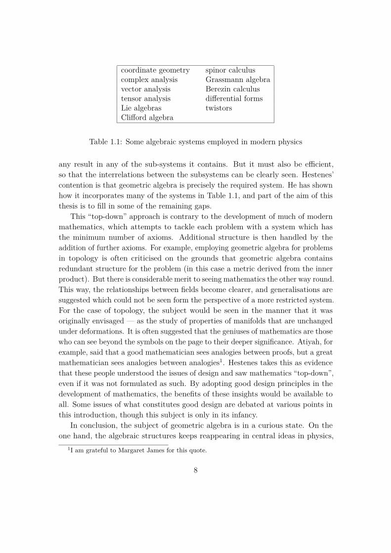
coordinate geometry spinor calculuscomplex analysis Grassmann algebravector analysis Berezin calculustensor analysis differential formsLie algebras twistorsClifford algebra

Table 1.1: Some algebraic systems employed in modern physics

any result in any of the sub-systems it contains. But it must also be efficient,so that the interrelations between the subsystems can be clearly seen. Hestenes’contention is that geometric algebra is precisely the required system. He has shownhow it incorporates many of the systems in Table 1.1, and part of the aim of thisthesis is to fill in some of the remaining gaps.

This “top-down” approach is contrary to the development of much of modernmathematics, which attempts to tackle each problem with a system which hasthe minimum number of axioms. Additional structure is then handled by theaddition of further axioms. For example, employing geometric algebra for problemsin topology is often criticised on the grounds that geometric algebra containsredundant structure for the problem (in this case a metric derived from the innerproduct). But there is considerable merit to seeing mathematics the other way round.This way, the relationships between fields become clearer, and generalisations aresuggested which could not be seen form the perspective of a more restricted system.For the case of topology, the subject would be seen in the manner that it wasoriginally envisaged — as the study of properties of manifolds that are unchangedunder deformations. It is often suggested that the geniuses of mathematics are thosewho can see beyond the symbols on the page to their deeper significance. Atiyah, forexample, said that a good mathematician sees analogies between proofs, but a greatmathematician sees analogies between analogies1. Hestenes takes this as evidencethat these people understood the issues of design and saw mathematics “top-down”,even if it was not formulated as such. By adopting good design principles in thedevelopment of mathematics, the benefits of these insights would be available toall. Some issues of what constitutes good design are debated at various points inthis introduction, though this subject is only in its infancy.

In conclusion, the subject of geometric algebra is in a curious state. On theone hand, the algebraic structures keeps reappearing in central ideas in physics,

1I am grateful to Margaret James for this quote.

8

geometry and topology, and most mathematicians are now aware of the importanceof Clifford algebras. On the other, there is far less support for Hestenes’ contentionthat geometric algebra, built on the framework of Clifford algebra, provides aunified language for much of modern mathematics. The work in this thesis isintended to offer support for Hestenes’ ideas.

1.2 Axioms and DefinitionsThe remaining sections of this chapter form an introduction to geometric algebraand to the conventions adopted in this thesis. Further details can be foundin “Clifford algebra to geometric calculus” [24], which is the most detailed andcomprehensive text on geometric algebra. More pedagogical introductions areprovided by Hestenes [25, 26] and Vold [44, 45], and [30] contains useful additionalmaterial. The conference report on the second workshop on “Clifford algebras andtheir applications in mathematical physics” [46] contains a review of the subjectand ends with a list of recommended texts, though not all of these are relevant tothe material in this thesis.

In deciding how best to define geometric algebra we arrive at our first issue ofmathematical design. Modern mathematics texts (see “Spin Geometry” by H.BLawson and M.-L. Michelsohn [15], for example) favour the following definition of aClifford algebra. One starts with a vector space V over a commutative field k, andsupposes that q is a quadratic form on V . The tensor algebra of V is defined as

T (V ) =∞∑r=0⊗rV, (1.5)

where ⊗ is the tensor product. One next defines an ideal Iq(V ) in T (V ) generatedby all elements of the form v ⊗ v + q(v)1 for v ∈ V . The Clifford algebra is thendefined as the quotient

Cl(V, q) ≡ T (V )/Iq(V ). (1.6)

This definition is mathematically correct, but has a number of drawbacks:

1. The definition involves the tensor product, ⊗, which has to be defined initially.

2. The definition uses two concepts, tensor algebras and ideals, which areirrelevant to the properties of the resultant geometric algebra.

3. Deriving the essential properties of the Clifford algebra from (1.6) requires

9

further work, and none of these properties are intuitively obvious from theaxioms.

4. The definition is completely useless for introducing geometric algebra to aphysicist or an engineer. It contains too many concepts that are the preserveof pure mathematics.

Clearly, it is desirable to find an alternative axiomatic basis for geometric algebrawhich does not share these deficiencies. The axioms should be consistent with ourideas of what constitutes good design. The above considerations lead us proposethe following principle:

The axioms of an algebraic system should deal directly with the objectsof interest.

That is to say, the axioms should offer some intuitive feel of the properties of thesystem they are defining.

The central properties of a geometric algebra are the grading, which separatesobjects into different types, and the associative product between the elements of thealgebra. With these in mind, we adopt the following definition. A geometric algebraG is a graded linear space, the elements of which are called multivectors. Thegrade-0 elements are called scalars and are identified with the field of real numbers(we will have no cause to consider a geometric algebra over the complex field). Thegrade-1 elements are called vectors, and can be thought of as directed line segments.The elements of G are defined to have an addition, and each graded subspace isclosed under this. A product is also defined which is associative and distributive,though non-commutative (except for multiplication by a scalar). The final axiom(which distinguishes a geometric algebra from other associative algebras) is thatthe square of any vector is a scalar.

Given two vectors, a and b, we find that

(a+ b)2 = (a+ b)(a+ b)= a2 + (ab+ ba) + b2. (1.7)

It follows thatab+ ba = (a+ b)2 − a2 − b2 (1.8)

and hence that (ab+ ba) is also a scalar. The geometric product of 2 vectors a, b

10

can therefore be decomposed as

ab = a·b+ a∧b, (1.9)

wherea·b ≡ 1

2(ab+ ba) (1.10)

is the standard scalar, or inner, product (a real scalar), and

a∧b ≡ 12(ab− ba) (1.11)

is the antisymmetric outer product of two vectors, originally introduced by Grass-mann. The outer product of a and b anticommutes with both a and b,

a(a∧b) = 12(a2b− aba)

= 12(ba2 − aba)

= −12(ab− ba)a

= −(a∧b)a, (1.12)

so a∧b cannot contain a scalar component. The axioms are also sufficient to showthat a∧b cannot contain a vector part. If we supposed that a∧b contained a vectorpart c, then the symmetrised product of a ∧ b with c would necessarily containa scalar part. But c(a ∧ b) + (a ∧ b)c anticommutes with any vector d satisfyingd·a = d·b = d·c = 0, and so cannot contain a scalar component. The result ofthe outer product of two vectors is therefore a new object, which is defined to begrade-2 and is called a bivector. It can be thought of as representing a directedplane segment containing the vectors a and b. The bivectors form a linear space,though not all bivectors can be written as the exterior product of two vectors.

The definition of the outer product is extended to give an inductive definition ofthe grading for the entire algebra. The procedure is illustrated as follows. Introducea third vector c and write

c(a∧b) = 12c(ab− ba)

= (a·c)b− (b·c)a− 12(acb− bca)

= 2(a·c)b− 2(b·c)a+ 12(ab− ba)c, (1.13)

so thatc(a∧b)− (a∧b)c = 2(a·c)b− 2(b·c)a. (1.14)

11

The right-hand side of (1.14) is a vector, so one decomposes c(a∧b) into

c(a∧b) = c·(a∧b) + c∧(a∧b) (1.15)

wherec·(a∧b) ≡ 1

2 [c(a∧b)− (a∧b)c] (1.16)

andc∧(a∧b) ≡ 1

2 [c(a∧b) + (a∧b)c] . (1.17)

The definitions (1.16) and (1.17) extend the definitions of the inner and outerproducts to the case where a vector is multiplying a bivector. Again, (1.17) resultsin a new object, which is assigned grade-3 and is called a trivector. The axioms aresufficient to prove that the outer product of a vector with a bivector is associative:

c∧(a∧b) = 12 [c(a∧b) + (a∧b)c]

= 14 [cab− cba+ abc− bac]

= 14 [2(c∧a)b+ acb+ abc+ 2b(c∧a)− bca− cba]

= 12 [(c∧a)b+ b(c∧a) + a(b·c)− (b·c)a]

= (c∧a)∧b. (1.18)

The definitions of the inner and outer products are extended to the geometricproduct of a vector with a grade-r multivector Ar as,

aAr = a·Ar + a∧Ar (1.19)

where the inner product

a·Ar ≡ 〈aAr〉r−1 = 12(aAr − (−1)rAra) (1.20)

lowers the grade of Ar by one and the outer (exterior) product

a∧Ar ≡ 〈aAr〉r+1 = 12(aAr + (−1)rAra) (1.21)

raises the grade by one. We have used the notation 〈A〉r to denote the result ofthe operation of taking the grade-r part of A (this is a projection operation). As afurther abbreviation we write the scalar (grade 0) part of A simply as 〈A〉.

The entire multivector algebra can be built up by repeated multiplicationof vectors. Multivectors which contain elements of only one grade are termed

12

homogeneous, and will usually be written as Ar to show that A contains only agrade-r component. Homogeneous multivectors which can be expressed purely asthe outer product of a set of (independent) vectors are termed blades.

The geometric product of two multivectors is (by definition) associative, and fortwo homogeneous multivectors of grade r and s this product can be decomposedas follows:

ArBs = 〈AB〉r+s + 〈AB〉r+s−2 . . .+ 〈AB〉|r−s|. (1.22)

The “·” and “∧” symbols are retained for the lowest-grade and highest-grade termsof this series, so that

Ar ·Bs ≡ 〈AB〉|s−r| (1.23)Ar∧Bs ≡ 〈AB〉s+r, (1.24)

which we call the interior and exterior products respectively. The exterior productis associative, and satisfies the symmetry property

Ar∧Bs = (−1)rsBs∧Ar. (1.25)

An important operation which can be performed on multivectors is reversion,which reverses the order of vectors in any multivector. The result of reversing themultivector A is written A, and is called the reverse of A. The reverse of a vectoris the vector itself, and for a product of multivectors we have that

(AB) = BA. (1.26)

It can be checked that for homogeneous multivectors

Ar = (−1)r(r−1)/2Ar. (1.27)

It is useful to define two further products from the geometric product. The firstis the scalar product

A∗B ≡ 〈AB〉. (1.28)

This is commutative, and satisfies the useful cyclic-reordering property

〈A . . . BC〉 = 〈CA . . . B〉. (1.29)

13

In positive definite spaces the scalar product defines the modulus function

|A| ≡ (A∗A)1/2. (1.30)

The second new product is the commutator product, defined by

A×B ≡ 12(AB −BA). (1.31)

The associativity of the geometric product ensures that the commutator productsatisfies the Jacobi identity

A×(B×C) +B×(C×A) + C×(A×B) = 0. (1.32)

Finally, we introduce an operator ordering convention. In the absence of brackets,inner, outer and scalar products take precedence over geometric products. Thus a·bcmeans (a·b)c and not a·(bc). This convention helps to eliminate unruly numbers ofbrackets. Summation convention is also used throughout this thesis.

One can now derive a vast number of properties of multivectors, as is donein Chapter 1 of [24]. But before proceeding, it is worthwhile stepping back andlooking at the system we have defined. In particular, we need to see that theaxioms have produced a system with sensible properties that match our intuitionsabout physical space and geometry in general.

1.2.1 The Geometric ProductOur axioms have led us to an associative product for vectors, ab = a·b+ a∧b. Wecall this the geometric product. It has the following two properties:

• Parallel vectors (e.g. a and αa) commute, and the the geometric product ofparallel vectors is a scalar. Such a product is used, for example, when findingthe length of a vector.

• Perpendicular vectors (a, b where a·b = 0) anticommute, and the geometricproduct of perpendicular vectors is a bivector. This is a directed planesegment, or directed area, containing the vectors a and b.

Independently, these two features of the algebra are quite sensible. It is thereforereasonable to suppose that the product of vectors that are neither parallel norperpendicular should contain both scalar and bivector parts.

14

But what does it mean to add a scalar to a bivector?

This is the point which regularly causes the most confusion (see [47], forexample). Adding together a scalar and a bivector doesn’t seem right — they aredifferent types of quantities. But this is exactly what you do want addition to do.The result of adding a scalar to a bivector is an object that has both scalar andbivector parts, in exactly the same way that the addition of real and imaginarynumbers yields an object with both real and imaginary parts. We call this latterobject a “complex number” and, in the same way, we refer to a (scalar+ bivector)as a “multivector”, accepting throughout that we are combining objects of differenttypes. The addition of scalar and bivector does not result in a single new quantityin the same way as 2 + 3 = 5; we are simply keeping track of separate componentsin the symbol ab = a·b+ a∧b or z = x+ iy. This type of addition, of objects fromseparate linear spaces, could be given the symbol ⊕, but it should be evident fromour experience of complex numbers that it is harmless, and more convenient, toextend the definition of addition and use the ordinary + sign.

Further insights are gained by the construction of explicit algebras for finitedimensional spaces. This is achieved most simply through the introduction of anorthonormal frame of vectors σi satisfying

σi ·σj = δij (1.33)

orσiσj + σjσi = 2δij. (1.34)

This is the conventional starting point for the matrix representation theory of finiteClifford algebras [13, 48]. It is also the usual route by which Clifford algebrasenter particle physics, though there the σi are thought of as operators, andnot as orthonormal vectors. The geometric algebra we have defined is associativeand any associative algebra can be represented as a matrix algebra, so why notdefine a geometric algebra as a matrix algebra? There are a number of flawswith this approach, which Hestenes has frequently drawn attention to [26]. Theapproach fails, in particular, when geometric algebra is used to study projectivelyand conformally related geometries [31]. There, one needs to be able to movefreely between different dimensional spaces. Matrix representations are too rigid toachieve this satisfactorily. An example of this will be encountered shortly.

There is a further reason for preferring not to introduce Clifford algebras viatheir matrix representations. It is related to our second principle of good design,

15

which is that

the axioms af an algebraic system should not introduce redundant struc-ture.

The introduction of matrices is redundant because all geometrically meaningfulresults exist independently of any matrix representations. Quite simply, matricesare irrelevant for the development of geometric algebra.

The introduction of a basis set of n independent, orthonormal vectors σidefines a basis for the entire algebra generated by these vectors:

1, σi, σi∧σj, σi∧σj∧σk, . . . , σ1∧σ2 . . .∧σn ≡ I. (1.35)

Any multivector can now be expanded in this basis, though one of the strengths ofgeometric algebra is that it possible to carry out many calculations in a basis-freeway. Many examples of this will be presented in this thesis,

The highest-grade blade in the algebra (1.35) is given the name “pseudoscalar”(or directed volume element) and is of special significance in geometric algebra. Itsunit is given the special symbol I (or i in three or four dimensions). It is a pureblade, and a knowledge of I is sufficient to specify the vector space over which thealgebra is defined (see [24, Chapter 1]). The pseudoscalar also defines the dualityoperation for the algebra, since multiplication of a grade-r multivector by I resultsin a grade-(n− r) multivector.

1.2.2 The Geometric Algebra of the PlaneA 1-dimensional space has insufficient geometric structure to be interesting, so westart in two dimensions, taking two orthonormal basis vectors σ1 and σ2. Thesesatisfy the relations

(σ1)2 = 1 (1.36)(σ2)2 = 1 (1.37)

andσ1 ·σ2 = 0. (1.38)

The outer product σ1 ∧ σ2 represents the directed area element of the plane andwe assume that σ1, σ2 are chosen such that this has the conventional right-handedorientation. This completes the geometrically meaningful quantities that we can

16

make from these basis vectors:

1,scalar

σ1, σ2,vectors

σ1∧σ2.

bivector (1.39)

Any multivector can be expanded in terms of these four basis elements. Additionof multivectors simply adds the coefficients of each component. The interestingexpressions are those involving products of the bivector σ1∧σ2 = σ1σ2. We findthat

(σ1σ2)σ1 = −σ2σ1σ1 = −σ2,

(σ1σ2)σ2 = σ1(1.40)

andσ1(σ1σ2) = σ2

σ2(σ1σ2) = −σ1.(1.41)

The only other product to consider is the square of σ1∧σ2,

(σ1∧σ2)2 = σ1σ2σ1σ2 = −σ1σ1σ2σ2 = −1. (1.42)

These results complete the list of the products in the algebra. In order to becompletely explicit, consider how two arbitrary multivectors are multiplied. Let

A = a0 + a1σ1 + a2σ2 + a3σ1∧σ2 (1.43)B = b0 + b1σ1 + b2σ2 + b3σ1∧σ2, (1.44)

then we find thatAB = p0 + p1σ1 + p2σ2 + p3σ1∧σ2, (1.45)

wherep0 = a0b0 + a1b1 + a2b2 − a3b3,

p1 = a0b1 + a1b0 + a3b2 − a2b3,

p2 = a0b2 + a2b0 + a1b3 − a3b1,

p3 = a0b3 + a3b0 + a1b2 − a2b1.

(1.46)

Calculations rarely have to be performed in this detail, but this exercise does serveto illustrate how geometric algebras can be made intrinsic to a computer language.One can even think of (1.46) as generalising Hamilton’s concept of complex numbersas ordered pairs of real numbers.

The square of the bivector σ1∧σ2 is −1, so the even-grade elements z = x+yσ1σ2

17

form a natural subalgebra, equivalent to the complex numbers. Furthermore, σ1∧σ2

has the geometric effect of rotating the vectors σ1, σ2 in their own plane by90 clockwise when multiplying them on their left. It rotates vectors by 90anticlockwise when multiplying on their right. (This can be used to define theorientation of σ1 and σ2).

The equivalence between the even subalgebra and complex numbers revealsa new interpretation of the structure of the Argand diagram. From any vectorr = xσ1 + yσ2 we can form an even multivector z by

z ≡ σ1r = x+ Iy, (1.47)

whereI ≡ σ1σ2. (1.48)

There is therefore a one-to-one correspondence between points in the Arganddiagram and vectors in two dimensions,

r = σ1z, (1.49)

where the vector σ1 defines the real axis. Complex conjugation,

z∗ ≡ z = rσ1 = x− Iy, (1.50)

now appears as the natural operation of reversion for the even multivector z. Takingthe complex conjugate of z results in a new vector r∗ given by

r∗ = σ1z

= (zσ1)= (σ1rσ1)= σ1rσ1

= −σ2rσ2. (1.51)

We will shortly see that equation (1.51) is the geometric algebra representation of areflection in the σ1 axis. This is precisely what one expects for complex conjugation.

This identification of points on the Argand diagram with (Clifford) vectors givesadditional operational significance to complex numbers of the form exp(iθ). The

18

even multivector equivalent of this is exp(Iθ), and applied to z gives

eIθz = eIθσ1r

= σ1e−Iθr. (1.52)

But we can now remove the σ1, and work entirely in the (real) Euclidean plane.Thus

r′ = e−Iθr (1.53)

rotates the vector r anticlockwise through an angle θ. This can be verified fromthe fact that

e−Iθσ1 = (cos θ − sin θI)σ1 = cos θ σ1 + sin θσ2 (1.54)

ande−Iθσ2 = cos θ σ2 − sin θσ1. (1.55)

Viewed as even elements in the 2-dimensional geometric algebra, exponentials of“imaginaries” generate rotations of real vectors. Thinking of the unit imaginary asbeing a directed plane segment removes much of the mystery behind the usage ofcomplex numbers. Furthermore, exponentials of bivectors provide a very generalmethod for handling rotations in geometric algebra, as is shown in Chapter 3.

1.2.3 The Geometric Algebra of SpaceIf we now add a third orthonormal vector σ3 to our basis set, we generate thefollowing geometric objects:

1,scalar

σ1, σ2, σ3,3 vectors

σ1σ2, σ2σ3, σ3σ1,3 bivectors

area elements

σ1σ2σ3.

trivectorvolume element

(1.56)

From these objects we form a linear space of (1 + 3 + 3 + 1) = 8 = 23 dimensions.Many of the properties of this algebra are shared with the 2-dimensional case sincethe subsets σ1, σ2, σ2, σ3 and σ3, σ1 generate 2-dimensional subalgebras. Thenew geometric products to consider are

(σ1σ2)σ3 = σ1σ2σ3,

(σ1σ2σ3)σk = σk(σ1σ2σ3) (1.57)

19

and(σ1σ2σ3)2 = σ1σ2σ3σ1σ2σ3 = σ1σ2σ1σ2σ

23 = −1. (1.58)

These relations lead to new geometric insights:

• A simple bivector rotates vectors in its own plane by 90, but forms trivectors(volumes) with vectors perpendicular to it.

• The trivector σ1∧σ2∧σ3 commutes with all vectors, and hence with allmultivectors.

The trivector (pseudoscalar) σ1σ2σ3 also has the algebraic property of squaringto −1. In fact, of the eight geometrical objects, four have negative square, σ1σ2,σ2σ3, σ3σ1 and σ1σ2σ3. Of these, the pseudoscalar σ1σ2σ3 is distinguished byits commutation properties and in view of these properties we give it the specialsymbol i,

i ≡ σ1σ2σ3. (1.59)

It should be quite clear, however, that the symbol i is used to stand for a pseu-doscalar and therefore cannot be used for the commutative scalar imaginary used,for example, in quantum mechanics. Instead, the symbol j is used for this unin-terpreted imaginary, consistent with existing usage in engineering. The definition(1.59) will be consistent with our later extension to 4-dimensional spacetime.

The algebra of 3-dimensional space is the Pauli algebra familiar from quantummechanics. This can be seen by multiplying the pseudoscalar in turn by σ3, σ1 andσ2 to find

(σ1σ2σ3)σ3 = σ1σ2 = iσ3,

σ2σ3 = iσ1,

σ3σ1 = iσ2,

(1.60)

which is immediately identifiable as the algebra of Pauli spin matrices. But wehave arrived at this algebra from a totally different route, and the various elementsin it have very different meanings to those assigned in quantum mechanics. Since3-dimensional space is closest to our perception of the world, it is worth emphasisingthe geometry of this algebra in greater detail. A general multivector M consists ofthe components

M = α

scalar+ a

vector+ ib

bivector+ iβ

pseudoscalar(1.61)

20

a b

c

vectorscalar

a b

line segment plane segmentbivector

volume segmenttrivector

α a

Figure 1.1: Pictorial representation of the elements of the Pauli algebra.

where a ≡ akσk and b ≡ bkσk. The reason for writing spatial vectors in bold typeis to maintain a visible difference between spatial vectors and spacetime 4-vectors.This distinction will become clearer when we consider relativistic physics. Themeaning of the σk is always unambiguous, so these are not written in bold type.

Each of the terms in (1.61) has a separate geometric significance:

1. scalars are physical quantities with magnitude but no spatial extent. Examplesare mass, charge and the number of words in this thesis.

2. vectors have both a magnitude and a direction. Examples include relativepositions, displacements and velocities.

3. bivectors have a magnitude and an orientation. They do not have a shape. InFigure 1.2.3 the bivector a∧b is represented as a parallelogram, but any othershape could have been chosen. In many ways a circle is more appropriate,since it suggests the idea of sweeping round from the a direction to the b

direction. Examples of bivectors include angular momentum and any otherobject that is usually represented as an “axial” vector.

4. trivectors have simply a handedness and a magnitude. The handedness tellswhether the vectors in the product a∧b∧c form a left-handed or right-handed set. Examples include the scalar triple product and, more generally,alternating tensors.

These four objects are represented pictorially in Figure 1.2.3. Further details anddiscussions are contained in [25] and [44].

The space of even-grade elements of the Pauli algebra,

ψ = α + ib, (1.62)

21

is closed under multiplication and forms a representation of the quarternion algebra.Explicitly, identifying i, j, k with iσ1, −iσ2, iσ3 respectively, the usual quarternionrelations are recovered, including the famous formula

i2 = j2 = k2 = ijk = −1. (1.63)

The quaternion algebra sits neatly inside the geometric algebra of space and, seenin this way, the i, j and k do indeed generate 90 rotations in three orthogonaldirections. Unsurprisingly, this algebra proves to be ideal for representing arbitraryrotations in three dimensions.

Finally, for this section, we recover Gibbs’ cross product. Since the × and ∧symbols have already been assigned meanings, we will use the ⊥ symbol for theGibbs’ product. This notation will not be needed anywhere else in this thesis. TheGibbs’ product is given by an outer product together with a duality operation(multiplication by the pseudoscalar),

a ⊥ b ≡ −ia∧b. (1.64)

The duality operation in three dimensions interchanges a plane with a vectororthogonal to it (in a right-handed sense). In the mathematical literature thisoperation goes under the name of the Hodge dual. Quantities like a or b wouldconventionally be called “polar vectors”, while the “axial vectors” which result fromcross-products can now be seen to be disguised versions of bivectors. The vectortriple product a ⊥ (b ⊥ c) becomes −a·(b∧c), which is the 3-dimensional form ofan expression which is now legitimate in arbitrary dimensions. We therefore dropthe restriction of being in 3-dimensional space and write

a·(b∧c) = 12(ab∧c− b∧ca) (1.65)

= a·bc− a·cb (1.66)

where we have recalled equation (1.14).

1.2.4 Reflections and RotationsOne of the clearest illustrations of the power of geometric algebra is the way inwhich it deals with reflections and rotations. The key to this approach is that,given any unit vector n (n2 = 1), an arbitrary vector a can be resolved into parts

22

parallel and perpendicular to n,

a = n2a

= n(n·a+ n∧a)= a‖ + a⊥, (1.67)

where

a‖ = a·nn (1.68)a⊥ = nn∧a. (1.69)

The result of reflecting a in the hyperplane orthogonal to n is the vector a⊥ − a‖,which can be written as

a⊥ − a‖ = nn∧a− a·nn= −n·an− n∧an= −nan. (1.70)

This formula for a reflection extends to arbitrary multivectors. For example, ifthe vectors a and b are both reflected in the hyperplane orthogonal to n, then thebivector a∧b is reflected to

(−nan)∧(−nbn) = 12(nannbn− nbnnan)

= na∧bn. (1.71)

In three dimensions, the sign difference between the formulae for vectors andbivectors accounts for the different behaviour of “polar” and “axial” vectors underreflections.

Rotations are built from pairs of reflections. Taking a reflection first in thehyperplane orthogonal to n, and then in the hyperplane orthogonal to m, leads tothe new vector

−m(−nan)m = mnanm

= RaR (1.72)

whereR ≡ mn. (1.73)

23

n

-nan

b

a

Figure 1.2: A rotation composed of two reflections.

The multivector R is called a rotor. It contains only even-grade elements andsatisfies the identity

RR = RR = 1. (1.74)

Equation (1.74) ensures that the scalar product of two vectors is invariant underrotations,

(RaR)·(RbR) = 〈RaRRbR〉= 〈aRRbRR〉= 〈ab〉= a·b. (1.75)

As an example, consider rotating the unit vector a into another unit vectorb, leaving all vectors perpendicular to a and b unchanged. This is accomplishedby a reflection perpendicular to the unit vector half-way between a and b (seeFigure 1.2.4)

n ≡ (a+ b)/|a+ b|. (1.76)

This reflects a into −b. A second reflection is needed to then bring this to b, whichmust take place in the hyperplane perpendicular to b. Together, these give therotor

R = bn = 1 + ba

|a+ b|= 1 + ba√

2(1 + b·a), (1.77)

24

which represents a simple rotation in the a∧b plane. The rotation is written

b = RaR, (1.78)

and the inverse transformation is given by

a = RbR. (1.79)

The transformation a 7→ RaR is a very general way of handling rotations. Inderiving this transformation the dimensionality of the space of vectors was at nopoint specified. As a result, the transformation law works for all spaces, whateverdimension. Furthermore, it works for all types of geometric object, whatever grade.We can see this by considering the image of the product ab when the vectors a andb are both rotated. In this case, ab is rotated to

RaRRbR = RabR. (1.80)

In dimensions higher than 5, an arbitrary even element satisfying (1.74) doesnot necessarily map vectors to vectors and will not always represent a rotation.The name “rotor” is then retained only for the even elements that do give rise torotations. It can be shown that all (simply connected) rotors can be written in theform

R = ±eB/2, (1.81)

where B is a bivector representing the plane in which the rotation is taking place.(This representation for a rotor is discussed more fully in Chapter 3.) The quantity

b = eαB/2ae−αB/2 (1.82)

is seen to be a pure vector by Taylor expanding in α,

b = a+ αB ·a+ α2

2! B ·(B ·a) + · · · . (1.83)

The right-hand side of (1.83) is a vector since the inner product of a vector with abivector is always a vector (1.14). This method of representing rotations directlyin terms of the plane in which they take place is very powerful. Equations (1.54)and (1.55) illustrated this in two dimensions, where the quantity exp(−Iθ) wasseen to rotate vectors anticlockwise through an angle θ. This works because in two

25

dimensions we can always write

e−Iθ/2reIθ/2 = e−Iθr. (1.84)

In higher dimensions the double-sided (bilinear) transformation law (1.78) isrequired. This is much easier to use than a one-sided rotation matrix, becausethe latter becomes more complicated as the number of dimensions increases. Thisbecomes clearer in three dimensions. The rotor

R ≡ exp(−ia/2) = cos(|a|/2)− i a

|a|sin(|a|/2) (1.85)

represents a rotation of |a| = (a2)1/2 radians about the axis along the direction of a.This is already simpler to work with than 3×3 matrices. In fact, the representationof a rotation by (1.85) is precisely how rotations are represented in the quaternionalgebra, which is well-known to be advantageous in three dimensions. In higherdimensions the improvements are even more dramatic.

Having seen how individual rotors are used to represent rotations, we must lookat their composition law. Let the rotor R transform the unit vector a into a vectorb,

b = RaR. (1.86)

Now rotate b into another vector b′, using a rotor R′. This requires

b′ = R′bR′ = (R′R)a(R′R) (1.87)

so that the transformation is characterised by

R 7→ R′R, (1.88)

which is the (left-sided) group combination rule for rotors. It is immediately clearthat the product of two rotors is a third rotor,

R′R(R′R) = R′RRR′ = R′R′ = 1, (1.89)

so that the rotors do indeed form a (Lie) group.The usefulness of rotors provides ample justification for adding up terms of

different grades. The rotor R on its own has no geometric significance, which is tosay that no meaning should be attached to the individual scalar, bivector, 4-vector. . . parts of R. When R is written in the form R = ±eB/2, however, the bivector

26

B has clear geometric significance, as does the vector formed from RaR. Thisillustrates a central feature of geometric algebra, which is that both geometricallymeaningful objects (vectors, planes . . . ) and the elements that act on them (rotors,spinors . . . ) are represented in the same algebra.

1.2.5 The Geometric Algebra of SpacetimeAs a final example, we consider the geometric algebra of spacetime. This algebra issufficiently important to deserve its own name — spacetime algebra — which we willusually abbreviate to STA. The square of a vector is no longer positive definite, andwe say that a vector x is timelike, lightlike or spacelike according to whether x2 > 0,x2 = 0 or x2 < 0 respectively. Spacetime consists of a single independent timelikedirection, and three independent spacelike directions. The spacetime algebra isthen generated by a set of orthonormal vectors γµ, µ = 0 . . . 3, satisfying

γµ ·γν = ηµν = diag(+ − − −). (1.90)

(The significance of the choice of metric signature will be discussed in Chapter 4.)The full STA is 16-dimensional, and is spanned by the basis

1, γµ σk, iσk, iγµ, i. (1.91)

The spacetime bivectors σk, k = 1 . . . 3 are defined by

σk ≡ γkγ0. (1.92)

They form an orthonormal frame of vectors in the space relative to the γ0 direction.The spacetime pseudoscalar i is defined by

i ≡ γ0γ1γ2γ3 (1.93)

and, since we are in a space of even dimension, i anticommutes with all odd-gradeelements and commutes with all even-grade elements. It follows from (1.92) that

σ1σ2σ3 = γ1γ0γ2γ0γ3γ0 = γ0γ1γ2γ3 = i. (1.94)

The following geometric significance is attached to these relations. An inertialsystem is completely characterised by a future-pointing timelike (unit) vector. Wetake this to be the γ0 direction. This vector/observer determines a map between

27

spacetime vectors a = aµγµ and the even subalgebra of the full STA via

aγ0 = a0 + a (1.95)

where

a0 = a·γ0 (1.96)a = a∧γ0. (1.97)

The even subalgebra of the STA is isomorphic to the Pauli algebra of space definedin Section 1.2.3. This is seen from the fact that the σk = γkγ0 all square to +1,

σk2 = γkγ0γkγ0 = −γkγkγ0γ0 = +1, (1.98)

and anticommute,

σjσk = γjγ0γkγ0 = γkγjγ0γ0 = −γkγ0γjγ0 = −σkσj (j 6= k). (1.99)

There is more to this equivalence than simply a mathematical isomorphism. Theway we think of a vector is as a line segment existing for a period of time. It istherefore sensible that what we perceive as a vector should be represented by aspacetime bivector. In this way the algebraic properties of space are determined bythose of spacetime.

As an example, if x is the spacetime (four)-vector specifying the position ofsome point or event, then the “spacetime split” into the γ0-frame gives

xγ0 = t+ x, (1.100)

which defines an observer timet = x·γ0 (1.101)

and a relative position vectorx = x∧γ0. (1.102)

One useful feature of this approach is the way in which it handles Lorentz-scalar

28

quantities. The scalar x2 can be decomposed into

x2 = xγ0γ0x

= (t+ x)(t− x)= t2 − x2, (1.103)

which must also be a scalar. The quantity t2 − x2 is now seen to be automaticallyLorentz-invariant, without needing to consider a Lorentz transformation.

The split of the six spacetime bivectors into relative vectors and relative bivectorsis a frame/observer-dependent operation. This can be illustrated with the Faradaybivector F = 1

2Fµνγµ∧γν , which is a full, 6-component spacetime bivector. The

spacetime split of F into the γ0-system is achieved by separating F into partswhich anticommute and commute with γ0. Thus

F = E + iB, (1.104)

where

E = 12(F − γ0Fγ0) (1.105)

iB = 12(F + γ0Fγ0). (1.106)

Here, both E and B are spatial vectors, and iB is a spatial bivector. Thisdecomposes F into separate electric and magnetic fields, and the explicit appearanceof γ0 in the formulae for E and B shows that this split is observer-dependent. Infact, the identification of spatial vectors with spacetime bivectors has always beenimplicit in the physics of electromagnetism through formulae like Ek = Fk0.

The decomposition (1.104) is useful for constructing relativistic invariants fromthe E and B fields. Since F 2 contains only scalar and pseudoscalar parts, thequantity

F 2 = (E + iB)(E + iB)= E2 −B2 + 2iE ·B (1.107)

is Lorentz-invariant. It follows that both E2 −B2 and E ·B are observer-invariantquantities.

Equation (1.94) is an important geometric identity, which shows that relativespace and spacetime share the same pseudoscalar i. It also exposes the weakness

29

of the matrix-based approach to Clifford algebras. The relation

σ1σ2σ3 = i = γ0γ1γ2γ3 (1.108)

cannot be formulated in conventional matrix terms, since it would need to relatethe 2× 2 Pauli matrices to 4× 4 Dirac matrices. Whilst we borrow the symbolsfor the Dirac and Pauli matrices, it must be kept in mind that the symbols arebeing used in a quite different context — they represent a frame of orthonormalvectors rather than representing individual components of a single isospace vector.

The identification of relative space with the even subalgebra of the STA ne-cessitates developing a set of conventions which articulate smoothly between thetwo algebras. This problem will be dealt with in more detail in Chapter 4, thoughone convention has already been introduced. Relative (or spatial) vectors in theγ0-system are written in bold type to record the fact that in the STA they areactually bivectors. This distinguishes them from spacetime vectors, which are leftin normal type. No problems can arise for the σk, which are unambiguouslyspacetime bivectors, so these are also left in normal type. The STA will be returnedto in Chapter 4 and will then be used throughout the remainder of this thesis. Wewill encounter many further examples of its utility and power.

1.3 Linear AlgebraWe have illustrated a number of the properties of geometric algebra, and have givenexplicit constructions in two, three and four dimensions. This introduction to theproperties of geometric algebra is now concluded by developing an approach to thestudy of linear functions and non-orthonormal frames.

1.3.1 Linear Functions and the OutermorphismGeometric algebra offers many advantages when used for developing the theory oflinear functions. This subject is discussed in some detail in Chapter 3 of “Cliffordalgebra to geometric calculus” [24], and also in [2] and [30]. The approach isillustrated by taking a linear function f(a) mapping vectors to vectors in the samespace. This function in extended via outermorphism to act linearly on multivectorsas follows,

f(a∧b∧. . .∧c) ≡ f(a)∧f(b) . . .∧f(c). (1.109)

30

The underbar on f shows that f has been constructed from the linear function f .The definition (1.109) ensures that f is a grade-preserving linear function mappingmultivectors to multivectors.

An example of an outermorphism was encountered in Section 1.2.4, where weconsidered how multivectors behave under rotations. The action of a rotation on avector a was written as

R(a) = eB/2ae−B/2, (1.110)

where B is the plane(s) of rotation. The outermorphism extension of this is simply

R(A) = eB/2Ae−B/2. (1.111)

An important property of the outermorphism is that the outermorphism of theproduct of two functions in the product of the outermorphisms,

f [g(a)]∧f [g(b)] . . .∧f [g(c)] = f [g(a)∧g(b) . . .∧g(c)]= f [g(a∧b∧. . .∧c)]. (1.112)

To ease notation, the product of two functions will be written simply as f g(A), sothat (1.112) becomes

fg(a)∧fg(b) . . .∧fg(c) = f g(a∧b∧. . .∧c). (1.113)

The pseudoscalar of an algebra is unique up to a scale factor, and this is usedto define the determinant of a linear function via

det(f) ≡ f(I)I−1, (1.114)

so thatf(I) = det(f)I. (1.115)

This definition clearly illustrates the role of the determinant as the volume scalefactor. The definition also serves to give a very quick proof of one of the mostimportant properties of determinants. It follows from (1.113) that

f g(I) = f(det(g)I)= det(g)f(I)= det(f) det(g)I (1.116)

31

and hence thatdet(fg) = det(f) det(g). (1.117)

This proof of the product rule for determinants illustrates our third (and final)principle of good design:

Definitions should be chosen so that the most important theorems canbe proven most economically.

The definition of the determinant clearly satisfies this criteria. Indeed, it is nothard to see that all of the main properties of determinants follow quickly from(1.115).

The adjoint to f , written as f , is defined by

f(a) ≡ ei〈f(ei)a〉 (1.118)

where ei is an arbitrary frame of vectors, with reciprocal frame ei. A frame-invariant definition of the adjoint can be given using the vector derivative, but wehave chosen not to introduce multivector calculus until Chapter 5. The definition(1.118) ensures that

b·f(a) = a·(b·eif(ei))= a·f(b). (1.119)

A symmetric function is one for which f = f .The adjoint also extends via outermorphism and we find that, for example,

f(a∧b) = f(a)∧f(b)= ei∧eja·f(ei)b·f(ej)= 1

2ei∧ej

(a·f(ei)b·f(ej)− a·f(ej)b·f(ei)

)= 1

2ei∧ej(a∧b)·f(ej∧ei). (1.120)

By using the same argument as in equation (1.119), it follows that

〈f(A)B〉 = 〈Af(B)〉 (1.121)

32

for all multivectors A and B. An immediate consequence is that

det f = 〈I−1f(I)〉= 〈f(I−1)I〉= det f. (1.122)

Equation (1.121) turns out to be a special case of the more general formulae,

Ar ·f(Bs) = f [f(Ar)·Bs] r ≤ s

f(Ar)·Bs = f [Ar ·f(Bs)] r ≥ s,(1.123)

which are derived in [24, Chapter 3].As an example of the use of (1.123) we find that

f(f(AI)I−1) = AIf(I−1) = A det f, (1.124)

which is used to construct the inverse functions,

f−1(A) = det(f)−1f(AI)I−1

f−1(A) = det(f)−1I−1f(IA).

(1.125)

These equations show how the inverse function is constructed from a double-duality operation. They are also considerably more compact and efficient than anymatrix-based formula for the inverse.

Finally, the concept of an eigenvector is generalized to that of an eigenbladeAr, which is an r-grade blade satisfying

f(Ar) = αAr, (1.126)

where α is a real eigenvalue. Complex eigenvalues are in general not considered,since these usually loose some important aspect of the geometry of the function f .As an example, consider a function f satisfying

f(a) = b

f(b) = −a, (1.127)

for some pair of vectors a and b. Conventionally, one might write

f(a+ jb) = −j(a+ jb) (1.128)

33

and say that a+ bj is an eigenvector with eigenvalue −j. But in geometric algebraone can instead write

f(a∧b) = b∧(−a) = a∧b, (1.129)

which shows that a∧b is an eigenblade with eigenvalue +1. This is a geometricallymore useful result, since it shows that the a∧b plane is an invariant plane of f .The unit blade in this plane generates its own complex structure, which is the moreappropriate object for considering the properties of f .

1.3.2 Non-Orthonormal FramesAt various points in this thesis we will make use of non-orthonormal frames, so anumber of their properties are summarised here. From a set of n vectors ei, wedefine the pseudoscalar

En = e1∧e2∧. . .∧en. (1.130)

The set ei constitute a (non-orthonormal) frame provided En 6= 0. The reciprocalframe ei satisfies

ei ·ej = δij, (1.131)

and is constructed via [24, Chapter 1]

ei = (−1)i−1e1∧. . . ei . . .∧enEn, (1.132)

where the check symbol on ei signifies that this vector is missing from the product.En is the pseudoscalar for the reciprocal frame, and is defined by

En = en∧en−1∧. . .∧e1. (1.133)

The two pseudoscalars En and En satisfy

EnEn = 1, (1.134)

and henceEn = En/(En)2. (1.135)

The components of the vector a in the ei frame are given by a·ei, so that

a = (a·ei)ei, (1.136)

34

from which we find that

2a = 2a·eiei

= eiaei + aeie

i

= eiaei + na. (1.137)

The fact that eiei = n follows from (1.131) and (1.132). From (1.137) we find that

eiaei = (2− n)a, (1.138)

which extends for a multivector of grade r to give the useful results:

eiArei = (−1)r(n− 2r)Ar,

ei(ei ·Ar) = rAr, (1.139)ei(ei∧Ar) = (n− r)Ar.

For convenience, we now specialise to positive definite spaces. The resultsbelow are easily extended to arbitrary spaces through the introduction of a metricindicator function [28]. A symmetric metric tensor g can be defined by

g(ei) = ei, (1.140)

so that, as a matrix, it has components

gij = ei ·ej. (1.141)

Sinceg(En) = En, (1.142)

it follows from (1.115) that

det(g) = EnEn = |En|2. (1.143)

It is often convenient to work with the fiducial frame σk, which is theorthonormal frame determined by the ei via

ek = h(σk) (1.144)

where h is the unique, symmetric fiducial tensor. The requirement that h be

35

symmetric means that the σk frame must satisfy

σk ·ej = σj ·ek, (1.145)

which, together with orthonormality, defines a set of n2 equations that determinethe σk (and hence h) uniquely, up to permutation. These permutations only alterthe labels for the frame vectors, and do not re-define the frame itself. From (1.144)it follows that

ej ·ek = h(ej)·σk = δjk (1.146)

so thath(ej) = σj = σj. (1.147)

(We are working in a positive definite space, so σj = σj for the orthonormal frameσj.) It can now be seen that h is the “square-root” of g,

g(ej) = ej = h(σj) = h2(ej). (1.148)

It follows thatdet(h) = |En|. (1.149)

The fiducial tensor, together with other non-symmetric square-roots of the metrictensor, find many applications in the geometric calculus approach to differentialgeometry [28]. We will also encounter a similar object in Chapter 7.

We have now seen that geometric algebra does indeed offer a natural languagefor encoding many of our geometric perceptions. Furthermore, the formulae forreflections and rotations have given ample justification to the view that the Cliffordproduct is a fundamental aspect of geometry. Explicit construction in two, threeand four dimensions has shown how geometric algebra naturally encompasses themore restricted algebraic systems of complex and quaternionic numbers. It shouldalso be clear from the preceding section that geometric algebra encompasses bothmatrix and tensor algebra. The following three chapters are investigations intohow geometric algebra encompasses a number of further algebraic systems.

36

Chapter 2

Grassmann Algebra and BerezinCalculus

This chapter outlines the basis of a translation between Grassmann calculus andgeometric algebra. It is shown that geometric algebra is sufficient to formulate allof the required concepts, thus integrating them into a single unifying framework.The translation is illustrated with two examples, the “Grauss integral” and the“Grassmann Fourier transform”. The latter demonstrates the full potential of thegeometric algebra approach. The chapter concludes with a discussion of somefurther developments and applications. Some of the results presented in this chapterfirst appeared in the paper “Grassmann calculus, pseudoclassical mechanics andgeometric algebra” [1].

2.1 Grassmann Algebra versus Clifford AlgebraThe modern development of mathematics has led to the popularly held view thatGrassmann algebra is more fundamental than Clifford algebra. This view is basedon the idea (recall Section 1.2) that a Clifford algebra is the algebra of a quadraticform. But, whilst it is true that every (symmetric) quadratic form defines a Cliffordalgebra, it is certainly not true that the usefulness of geometric algebra is restrictedto metric spaces. Like all mathematical systems, geometric algebra is subject tomany different interpretations, and the inner product need not be related to theconcepts of metric geometry. This is best illustrated by a brief summary of howgeometric algebra is used in the study of projective geometry.

In projective geometry [31], points are labeled by vectors, a, the magnitude

37

of which is unimportant. That is, points in a projective space of dimension n− 1are identified with rays in a space of dimension n which are solutions of theequation x ∧ a = 0. Similarly, lines are represented by bivector blades, planes bytrivectors, and so on. Two products (originally defined by Grassmann) are neededto algebraically encode the principle concepts of projective geometry. These arethe progressive and regressive products, which encode the concepts of the join andthe meet respectively. The progressive product of two blades is simply the outerproduct. Thus, for two points a and b, the line joining them together is representedprojectively by the bivector a∧b. If the grades of Ar and Bs sum to more than nand the vectors comprising Ar and Bs span n-dimensional space, then the join isthe pseudoscalar of the space. The regressive product, denoted ∨, is built fromthe progressive product and duality. Duality is defined as (right)-multiplication bythe pseudoscalar, and is denoted A∗r. For two blades Ar and Bs, the meet is thendefined by

(Ar ∨Bs)∗ = A∗r∧B∗s (2.1)

⇒ Ar ∨Bs = A∗r ·Bs. (2.2)

It is implicit here that the dual is taken with respect to the join of Ar and Bs. Asan example, in two-dimensional projective geometry (performed in the geometricalgebra of space) the point of intersection of the lines given by A and B, where

A = ai (2.3)B = bi, (2.4)

is given by the pointA ∨B = −a·B = −ia∧b. (2.5)

The definition of the meet shows clearly that it is most simply formulated interms of the inner product, yet no metric geometry is involved. It is probablyunsurprising to learn that geometric algebra is ideally suited to the study ofprojective geometry [31]. It is also well suited to the study of determinants andinvariant theory [24], which are also usually thought to be the preserve of Grassmannalgebra [49, 50]. For these reasons there seems little point in maintaining a rigiddivision between Grassmann and geometric algebra. The more fruitful approach isto formulate the known theorems from Grassmann algebra in the wider language ofgeometric algebra. There they can be compared with, and enriched by, developmentsfrom other subjects. This program has been largely completed by Hestenes, Sobczykand Ziegler [24, 31]. This chapter addresses one of the remaining subjects — the

38

“calculus” of Grassmann variables introduced by Berezin [35].Before reaching the main content of this chapter, it is necessary to make a few

comments about the use of complex numbers in applications of Grassmann variables(particularly in particle physics). We saw in Sections 1.2.2 and 1.2.3 that within the2-dimensional and 3-dimensional real Clifford algebras there exist multivectors thatnaturally play the rôle of a unit imaginary. Similarly, functions of several complexvariables can be studied in a real 2n-dimensional algebra. Furthermore, in Chapter 4we will see how the Schrödinger, Pauli and Dirac equations can all be given realformulations in the algebras of space and spacetime. This leads to the speculationthat a scalar unit imaginary may be unnecessary for fundamental physics. Often,the use of a scalar imaginary disguises some more interesting geometry, as is thecase for imaginary eigenvalues of linear transformations. However, there are cases inmodern mathematics where the use of a scalar imaginary is entirely superfluous tocalculations. Grassmann calculus is one of these. Accordingly, the unit imaginaryis dropped in what follows, and an entirely real formulation is given.

2.2 The Geometrisation of Berezin CalculusThe basis of Grassmann/Berezin calculus is described in many sources. Berezin’s“The method of second quantisation” [35] is one of the earliest and most citedtexts, and a useful summary of the main results from this is contained in theAppendices to [39]. More recently, Grassmann calculus has been extended to thefield of superanalysis [51, 52], as well as in other directions [53, 54].

The basis of the approach adopted here is to utilise the natural embedding ofGrassmann algebra within geometric algebra, thus reversing the usual progressionfrom Grassmann to Clifford algebra via quantization. We start with a set of nGrassmann variables ζi, satisfying the anticommutation relations

ζi, ζj = 0. (2.6)

The Grassmann variables ζi are mapped into geometric algebra by introducing aset of n independent Euclidean vectors ei, and replacing the product of Grassmannvariables by the exterior product,

ζiζj ↔ ei ∧ ej. (2.7)

39

Equation (2.6) is now satisfied by virtue of the antisymmetry of the exterior product,

ei∧ej + ej∧ei = 0. (2.8)

In this way any combination of Grassmann variables can be replaced by a multivec-tor. Nothing is said about the interior product of the ei vectors, so the ei frameis completely arbitrary.

In order for the above scheme to have computational power, we need a translationfor for the calculus introduced by Berezin [35]. In this calculus, differentiation isdefined by the rules

∂ζj∂ζi

= δij, (2.9)

ζj

←−∂

∂ζi= δij, (2.10)

together with the “graded Leibnitz rule”,

∂

∂ζi(f1f2) = ∂f1

∂ζif2 + (−1)[f1]f1

∂f2

∂ζi, (2.11)

where [f1] is the parity of f1. The parity of a Grassmann variable is determinedby whether it contains an even or odd number of vectors. Berezin differentiationis handled within the algebra generated by the ei frame by introducing thereciprocal frame ei, and replacing

∂

∂ζi( ↔ ei ·( (2.12)

so that∂ζj∂ζi

↔ ei ·ej = δij. (2.13)

It should be remembered that upper and lower indices are used to distinguish aframe from its reciprocal frame, whereas Grassmann algebra only uses these indicesto distinguish metric signature.

The graded Leibnitz rule follows simply from the axioms of geometric algebra.For example, if f1 and f2 are grade-1 and so translate to vectors a and b, then therule (2.11) becomes

ei ·(a∧b) = ei ·ab− aei ·b, (2.14)

40

which is simply equation (1.14) again.Right differentiation translates in a similar manner,

)←−∂

∂ζi↔ )·ei, (2.15)

and the standard results for Berezin second derivatives [35] can also be verifiedsimply. For example, given that F is the multivector equivalent of the Grassmannvariable f(ζ),

∂

∂ζi

∂

∂ζjf(ζ) ↔ ei ·(ej ·F ) = (ei∧ej)·F

= −ej ·(ei ·F ) (2.16)

shows that second derivatives anticommute, and(∂f

∂ζi

) ←−∂

∂ζj↔ (ei ·F )·ej = ei ·(F ·ej) (2.17)

shows that left and right derivatives commute.The final concept needed is that of integration over a Grassmann algebra. In

Berezin calculus, this is defined to be the same as right differentiation (apartperhaps from some unimportant extra factors of j and 2π [52]), so that

∫f(ζ)dζndζn−1 . . . dζ1 ≡ f(ζ)

←−∂

∂ζn

←−∂

∂ζn−1. . .

←−∂

∂ζ1. (2.18)

These translate in exactly the same way as the right derivative (2.12). The onlyimportant formula is that for the total integral∫

f(ζ)dζndζn−1 . . . dζ1 ↔ (. . . ((F ·en)·en−1) . . .)·e1 = 〈FEn〉, (2.19)

where again F is the multivector equivalent of f(ζ), as defined by (2.6). Equation(2.19) picks out the coefficient of the pseudoscalar part of F since, if 〈F 〉n is givenby αEn, then

〈FEn〉 = α. (2.20)

Thus the Grassman integral simply returns the coefficient α.

41

A change of variables is performed by a linear transformation f , say, with

e′i = f(ei) (2.21)

⇒ E ′n = f(En) = det(f)En. (2.22)

But the ei must transform under f−1 to preserve orthonormality, so

ei′ = f

−1(ei) (2.23)

⇒ En′ = det(f)−1En, (2.24)

which recovers the usual result for a change of variables in a Grassmann multipleintegral. That E ′nEn′ = 1 follows from the definitions above.

In the above manner all the basic formulae of Grassmann calculus can bederived in geometric algebra, and often these derivations are simpler. Moreover,they allow for the results of Grassmann algebra to be incorporated into a widerscheme, where they may find applications in other fields. As a further comment,this translation also makes it clear why no measure is associated with Grassmannintegrals: nothing is being added up!

2.2.1 Example I. The “Grauss” IntegralThe Grassmann analogue of the Gaussian integral [35],∫

exp12a

jkζjζk dζn . . . dζ1 = det(a)1/2, (2.25)

where ajk is an antisymmetric matrix, is one of the most important results inapplications of Grassmann algebra. This result is used repeatedly in fermionicpath integration, for example. It is instructive to see how (2.25) is formulated andproved in geometric algebra. First, we translate

12a

jkζjζk ↔ 12a

jkej∧ek = A, say, (2.26)

where A is a general bivector. The integral now becomes∫

exp12a

jkζjζk dζn . . . dζ1 ↔ 〈(1 + A+ A∧A2! + . . .)En〉. (2.27)

42

It is immediately clear that (2.27) is only non-zero for even n (= 2m say), in whichcase (2.27) becomes

〈(1 + A+ A∧A2! + . . .)En〉 = 1

m!〈(A)mEn〉. (2.28)

This type of expression is considered in Chapter 3 of [24] in the context of theeigenvalue problem for antisymmetric functions. This provides a good illustration ofhow the systematic use of a unified language leads to analogies between previouslyseparate results.

In order to prove that (2.28) equals det(a)1/2 we need the result that, in spaceswith Euclidean or Lorentzian signature, any bivector can be written, not necessarilyuniquely, as a sum of orthogonal commuting blades. This is proved in [24, Chapter3]. Using this result, we can write A as

A = α1A1 + α2A2 + . . . αmAm, (2.29)

where

Ai ·Aj = −δij (2.30)[Ai, Aj] = 0 (2.31)

A1A2 . . . Am = I. (2.32)

Equation (2.28) now becomes,

〈(α1α2 . . . αm)IEn〉 = det(g)−1/2α1α2 . . . αm, (2.33)

where g is the metric tensor associated with the ei frame (1.140).If we now introduce the function

f(a) = a·A, (2.34)

we find that [24, Chapter 3]

f(a∧b) = (a·A)∧(b·A)= 1

2(a∧b)·(A∧A)− (a∧b)·AA. (2.35)

43

It follows that the Ai blades are the eigenblades of f , with

f(Ai) = α2iAi, (2.36)

and hencef(I) = f(A1∧A2∧. . . Am) = (α1α2 . . . αm)2I (2.37)

⇒ det(f) = (α1α2 . . . αm)2. (2.38)

In terms of components, however,

fkj = ej ·f(ek)= gjla

lk, (2.39)

⇒ det(f) = det(g) det(a). (2.40)

Inserting (2.40) into (2.33), we have

1m!〈(A)mEn〉 = det(a)1/2, (2.41)

as required.This result can be derived more succinctly using the fiducial frame σi = h−1(ei)

to write (2.27) as1m!〈(A

′)mI〉, (2.42)

where A′ = 12a

jkσjσk. This automatically takes care of the factors of det(g)1/2,though it is instructive to note how these appear naturally otherwise.

2.2.2 Example II. The Grassmann Fourier TransformWhilst the previous example did not add much new algebraically, it did serveto demonstrate that notions of Grassmann calculus were completely unnecessaryfor the problem. In many other applications, however, the geometric algebraformulation does provide for important algebraic simplifications, as is demonstratedby considering the Grassmann Fourier transform.

In Grassmann algebra one defines Fourier integral transformations betweenanticommuting spaces ζk and ρk by [39]

G(ζ) =∫

expj∑ ζkρkH(ρ)dρn . . . dρ1

H(ρ) = εn∫

exp−j∑ ζkρkG(ζ)dζn . . . dζ1,

(2.43)

44

where εn = 1 for n even and j for n odd. The factors of j are irrelevant and can bedropped, so that (2.43) becomes

G(ζ) =∫

exp∑ ζkρkH(ρ)dρn . . . dρ1

H(ρ) = (−1)n∫

exp−∑ ζkρkG(ζ)dζn . . . dζ1.

(2.44)

These expressions are translated into geometric algebra by introducing a pair ofanticommuting copies of the same frame, ek, fk, which satisfy

ej ·ek = fj ·fk (2.45)ej ·fk = 0. (2.46)

The full set ek, fk generate a 2n-dimensional Clifford algebra. The translationnow proceeds by replacing

ζk ↔ ek,

ρk ↔ fk,(2.47)

where the ρk have been replaced by elements of the reciprocal frame fk. From(2.45), the reciprocal frames must also satisfy

ej ·ek = f j ·fk. (2.48)

We next define the bivector (summation convention implied)

J = ej∧f j = ej∧fj. (2.49)

The equality of the two expressions for J follows from (2.45),

ej∧f j = (ej ·ek)ek∧f j

= (fj ·fk)ek∧f j

= ek∧fk. (2.50)

The bivector J satisfies

ej ·J = fj fj ·J = −ej,ej ·J = f j f j ·J = −ej, (2.51)

and it follows that(a·J)·J = −a, (2.52)

45

for any vector a in the 2n-dimensional algebra. Thus J generates a complexstructure, which on its own is sufficient reason for ignoring the scalar j. Equation(2.52) can be extended to give

e−Jθ/2aeJθ/2 = cos θ a+ sin θ a·J, (2.53)

from which it follows that expJπ/2 anticommutes with all vectors. Consequently,this quantity can only be a multiple of the pseudoscalar and, since expJπ/2 hasunit magnitude, we can define the orientation such that

eJπ/2 = I. (2.54)

This definition ensures that

EnFn = EnFn = I. (2.55)

Finally, we introduce the notation

Ck = 1k!〈J

k〉2k. (2.56)

The formulae (2.44) now translate to

G(e) =n∑j=0

(Cj∧H(f))·Fn

H(f) = (−1)nn∑j=0

(Cj∧G(e))·En, (2.57)

where the convention is adopted that terms where Cj∧H or Cj∧G have grade lessthan n do not contribute. Since G and H only contain terms purely constructedfrom the ek and fk respectively, (2.57) can be written as

G(e) =n∑j=0

(Cn−j∧〈H(f)〉j)·Fn

H(f) =n∑j=0

(−1)j(〈G(e)〉j∧Cn−j)·En. (2.58)

So far we have only derived a formula analogous to (2.44), but we can now go

46

much further. By using

eJθ = cosn θ + cosn−1 θ sin θ C1 + . . .+ sinn θ I (2.59)

to decompose eJ(θ+π/2) = eJθI in two ways, it can be seen that

Cn−r = (−1)rCrI = (−1)rICr, (2.60)

and hence (using some simple duality relations) (2.58) become

G(e) =n∑j=0

Cj ·HjEn

H(f) = (−1)nn∑j=0

Gj ·CjF n. (2.61)

Finally, since G and H are pure in the ek and fk respectively, the effect ofdotting with Ck is simply to interchange each ek for an −fk and each fk for an ek.For vectors this is achieved by dotting with J . But, from (2.53), the same result isachieved by a rotation through π/2 in the planes of J . Rotations extend simplyvia outermorphism, so we can now write

Cj ·Hj = eJπ/4Hje−Jπ/4

Gj ·Cj = e−Jπ/4GjeJπ/4. (2.62)

We thus arrive at the following equivalent expressions for (2.57):

G(e) = eJπ/4H(f)e−Jπ/4EnH(f) = (−1)ne−Jπ/4G(e)eJπ/4F n. (2.63)

The Grassmann Fourier transformation has now been reduced to a rotation throughπ/2 in the planes specified by J , followed by a duality transformation. Proving the“inversion” theorem (i.e. that the above expressions are consistent) amounts to nomore than carrying out a rotation, followed by its inverse,

G(e) = eJπ/4((−1)ne−Jπ/4G(e)eJπ/4F n

)e−Jπ/4En

= G(e)EnEn = G(e). (2.64)

This proof is considerably simpler than any that can be carried out in the more

47

restrictive system of Grassmann algebra.

2.3 Some Further DevelopmentsWe conclude this chapter with some further observations. We have seen how mostaspects of Grassmann algebra and Berezin calculus can be formulated in terms ofgeometric algebra. It is natural to expect that other fields involving Grassmannvariables can also be reformulated (and improved) in this manner. For example,many of the structures studied by de Witt [52] (super-Lie algebras, super-Hilbertspaces) have natural multivector expressions, and the cyclic cohomology groups ofGrassmann algebras described by Coquereaux, Jadczyk and Kastler [53] can beformulated in terms of the multilinear function theory developed by Hestenes &Sobczyk [24, Chapter 3]. In Chapter 5 the formulation of this chapter is appliedGrassmann mechanics and the geometric algebra approach is again seen to offerconsiderable benefits. Further applications of Grassmann algebra are considered inChapter 3, in which a novel approach to the theory of linear functions is discussed.A clear goal for future research in this subject is to find a satisfactory geometricalgebra formulation of supersymmetric quantum mechanics and field theory. Somepreliminary observations on how such a formulation might be achieved are made inChapter 5, but a more complete picture requires further research.

As a final comment, it is instructive to see how a Clifford algebra is traditionallybuilt from the elements of Berezin calculus. It is well known [35] that the operators

Qk = ζk + ∂

∂ζk, (2.65)

satisfy the Clifford algebra generating relations

Qj, Qk = 2δjk, (2.66)

and this has been used by Sherry to provide an alternative approach to quantizing aGrassmann system [55, 56]. The geometric algebra formalism offers a novel insightinto these relations. By utilising the fiducial tensor, we can write

Qka(ζ) ↔ ek∧A+ ek ·A = h(σk)∧A+ h−1(σk)·A= h(σk∧h−1(A)) + h(sk ·h−1(A))= h[σkh−1(A)], (2.67)

48

where A is the multivector equivalent of a(ζ) and we have used (1.123). Theoperator Qk thus becomes an orthogonal Clifford vector (now Clifford multiplied),sandwiched between a symmetric distortion and its inverse. It is now simple to seethat

Qj, Qka(ζ) ↔ h(2σj ·σkh−1(A)) = 2δjkA. (2.68)

The above is an example of the ubiquity of the fiducial tensor in applicationsinvolving non-orthonormal frames. In this regard it is quite surprising that thefiducial tensor is not more prominent in standard expositions of linear algebra.

Berezin [35] defines dual operators to the Qk by

Pk = −j(ζk −∂

∂ζk), (2.69)

though a more useful structure is derived by dropping the j, and defining

Pk = ζk −∂

∂ζk. (2.70)

These satisfyPj, Pk = −2δjk (2.71)

andPj, Qk = 0, (2.72)

so that the Pk, Qk span a 2n-dimensional balanced algebra (signature n, n). The Pkcan be translated in the same manner as the Qk, this time giving (for a homogeneousmultivector)

Pka(ζ) ↔ ek∧Ar − ek ·Ar = (−1)rh[h−1(Ar)σk]. (2.73)

The σk frame now sits to the right of the multivector on which it operates. Thefactor of (−1)r accounts for the minus sign in (2.71) and for the fact that the leftand right multiples anticommute in (2.72). The Qk and Pk can both be given rightanalogues if desired, though this does not add anything new. The Qk and Pkoperators are discussed more fully in Chapter 4, where they are related to thetheory of the general linear group.

49

Chapter 3

Lie Groups and Spin Groups

This chapter demonstrates how geometric algebra provides a natural arena for thestudy of Lie algebras and Lie groups. In particular, it is shown that every matrixLie group can be realised as a spin group. Spin groups consist of even products ofunit magnitude vectors, and arise naturally from the geometric algebra treatmentof reflections and rotations (introduced in Section 1.2.4). The generators of a spingroup are bivectors, and it is shown that every Lie algebra can be represented bya bivector algebra. This brings the computational power of geometric algebra toapplications involving Lie groups and Lie algebras. An advantage of this approachis that, since the rotors and bivectors are all elements of the same algebra, thediscussion can move freely between the group and its algebra. The spin version ofthe general linear group is studied in detail, revealing some novel links with thestructures of Grassmann algebra studied in Chapter 2. An interesting result thatemerges from this work is that every linear transformation can be represented as a(geometric) product of vectors. Some applications of this result are discussed. Anumber of the ideas developed in this chapter appeared in the paper “Lie groupsas spin groups” [2].

Throughout this chapter, the geometric algebra generated by p independentvectors of positive norm and q of negative norm is denoted as <p,q. The grade-k subspace of this algebra is written as <kp,q and the space of vectors, <1

p,q, isabbreviated to <p,q. The Euclidean algebra <n,0 is abbreviated to <n, and thevector space <1

n is written as <n. Lie groups and their algebras are labeled accordingto the conventions of J.F. Cornwell’s “Group Theory in Physics”, Vol. 2 [57]. (Auseful table of these conventions is found on page 392).

50

3.1 Spin Groups and their GeneratorsIn this chapter we are interested in spin groups. These arise from the geometricalgebra representation of orthogonal transformations — linear functions on <p,qwhich preserve inner products. We start by considering the case of the Euclideanalgebra <n. The simplest orthogonal transformation of <n is a reflection in thehyperplane perpendicular to some unit vector n,

n(a) = −nan, (3.1)

where we have recalled equation (1.70). (A convenient feature of the under-bar/overbar notation for linear functions is that a function can be written in termsof the multivector that determines it.) The function n satisfies

n(a)·n(b) = 〈nannbn〉 = a·b, (3.2)

and so preserves the inner product. On combining n with a second reflection m,where

m(a) = −mam, (3.3)

the functionmn(a) = mnanm (3.4)

is obtained. This function also preserves inner products, and in Section 1.2.4 wasidentified as a rotation in the m∧n plane. The group of even products of unitvectors is denoted spin(n). It consists of all even multivectors (rotors) satisfying

RR = 1 (3.5)

and such that the quantity RaR is a vector for all vectors a. The double-sidedaction of a rotor R on a vector a is written as

R(a) = RaR (3.6)

and the R form the group of rotations on <n, denoted SO(n). The rotors afford aspin-1/2 description of rotations, hence rotor groups are referred to as spin groups.

In spaces with mixed signature the situation is slightly more complicated. Inorder to take care of the fact that a unit vector can now have n2 = ±1, equation (3.1)must be modified to

n(a) = −nan−1. (3.7)

51

Taking even combinations of reflections now leads to functions of the type

M(a) = MaM−1, (3.8)

as opposed to MaM . Again, the spin group spin(p, q) is defined as the group ofeven products of unit vectors, but its elements now satisfy MM = ±1. The term“rotor” is retained for elements of spin(p, q) satisfying RR = 1. The subgroup ofspin(p, q) containing just the rotors is called the rotor group (this is sometimeswritten as spin+(p, q) in the literature). The action of a rotor on a vector a isalways defined by (3.6). Spin groups and rotor groups are both Lie groups and, ina space with mixed signature, the spin group differs from the rotor group only bya direct product with an additional subgroup of discrete transformations.

The generators of a spin group are found by adapting the techniques found inany of the standard texts of Lie group theory (see [57], for example). We are onlyinterested in the subgroup of elements connected to the identity, so only need toconsider the rotor group. We introduce a one-parameter set of rotors R(t), so that

R(t)aR(t) = 〈R(t)aR(t)〉1 (3.9)

for all vectors a and for all values of the parameter t. On differentiating withrespect to t, we find that the quantity

R′aR +RaR′ = R′R(RaR) + (RaR)RR′

= R′R(RaR)− (RaR)R′R (3.10)

must be a vector, where we have used RR = 1 to deduce that

R′R = −RR′. (3.11)

The commutator of R′R with an arbitrary vector therefore results in a vector, soR′R can only contain a bivector part. (R′R cannot contain a scalar part, since(R′R) = −R′R.) The generators of a rotor group are therefore a set of bivectors inthe algebra containing the rotors.

A simple application of the Jacobi identity gives, for vectors a, b, c, and d,

(a∧b)×(c∧d) = [(a∧b)·c]∧d− [(a∧b)·d]∧c, (3.12)

so the commutator product of two bivector blades results in a third bivector. It

52

follows that the space of bivectors is closed under the commutator product, andhence that the bivectors (together with the commutator product) form the Liealgebra of a spin group. It should be noted that the commutator product, ×,in equation (3.12) differs from the commutator bracket by a factor of 1/2. Thecommutator product is simpler to use, since it is the bivector part of the fullgeometric product of two bivectors A and B:

AB = A·B + A×B + A∧B (3.13)

where

A·B + A∧B = 12(AB +BA), (3.14)

A×B = 12(AB −BA). (3.15)

For this reason the commutator product will be used throughout this chapter.Since the Lie algebra of a spin group is generated by the bivectors, it follows

that all rotors simply connected to the identity can be written in the form

R = eB/2, (3.16)

which ensures thatR = e−B/2 = R−1. (3.17)

The form of a rotor given by equation (3.16) was found in Section 1.2.4, whererotations in a single Euclidean plane were considered. The factor of 1/2 is includedbecause rotors provide a half-angle description of rotations. In terms of the Liealgebra, the factor of 1/2 is absorbed into our use of the commutator product, asopposed to the commutator bracket.

It can be shown that, in positive definite spaces, all rotors can be written inthe form of (3.16). The bivector B is not necessarily unique, however, as can beseen by considering the power series definition of the logarithm,

lnX = 2[H + H3

3 + H5

5 + · · · ] (3.18)

whereH = X − 1

X + 1 . (3.19)

It is implicit in this formula that 1 +X is invertible, and the logarithm will not

53

be well-defined if this is not the case. For example, the pseudoscalar I in <4,0 is arotor (II = 1), the geometric effect of which is to reverse the sign of all vectors.But 1 + I is not invertible, since (1 + I)2 = 2(1 + I). This manifests itself asa non-uniqueness in the logarithm of I — given any bivector blade B satisfyingB2 = −1, I can be written as

I = expB(1− I)π2 . (3.20)

Further problems can arise in spaces with mixed signature. In the spacetimealgebra, for example, whilst the rotor

R = (γ0 + γ1 − γ2)γ2 = 1 + (γ0 + γ1)γ2 (3.21)

can be written asR = exp(γ0 + γ1)γ2, (3.22)

the rotor−R = expγ1γ2

π

2 R = −1− (γ0 + γ1)γ2 (3.23)

cannot be written as the exponential of a bivector. The problem here is that theseries for ln(−X) is found by replacing H by H−1 in equation (3.18) and, whilst1 + R = 2 + (γ0 + γ1)γ2 is invertible, 1− R = −(γ0 + γ1)γ2 is null and thereforenot invertible.

Further examples of rotors with no logarithm can be constructed in spaceswith other signatures. Near the identity, however, the Baker-Campbell-Hausdorffformula ensures that, for suitably small bivectors, one can always write

eA/2eB/2 = eC/2. (3.24)

So, as is usual in Lie group theory, the bulk of the properties of the rotor (andspin) groups are transferred to the properties of their bivector generators.

In the study of Lie groups and their algebras, the adjoint representation playsa particularly important role. The adjoint representation of a spin group is formedfrom functions mapping the Lie algebra to itself,

AdM(B) ≡MBM−1 = M(B). (3.25)

The adjoint representation is therefore formed by the outermorphism action of the

54

linear functions M(a) = MaM−1. For the rotor subgroup, we have

AdR(B) = R(B) = RBR. (3.26)

It is immediately seen that the adjoint representation satisfies

AdM1 [AdM2(B)] = AdM1M2(B). (3.27)

The adjoint representation of the Lie group induces a representation of the Liealgebra as

adA/2(B) = A×B, (3.28)

oradA(B) = 2A×B. (3.29)

The Jacobi identity ensures that

12(adAadB − adBadA)(C) = 2[A×(B×C)−B×(A×C)]

= 2(A×B)×C= adA×B(C). (3.30)

The Killing form is constructed by considering adA as a linear operator on thespace of bivectors, and defining

K(A,B) = Tr(adAadB). (3.31)

For the case where the Lie algebra is the set of all bivectors, we can define a basisset of bivectors as BK = ei∧ej (i < j) with reciprocal basis BK = ej∧ei. Here, theindex K is a simplicial index running from 1 to n(n− 1)/2 over all combinationsof i and j with i < j. A matrix form of the adjoint representation is now given by

(adA)KJ = 2(A×BJ)·BK (3.32)

so that the Killing form becomes

K(A,B) = 4n(n−1)/2∑J,K=1

(A×BJ)·BK(B×BK)·BJ

= 2[A×(B×(ei∧ej))]·(ej∧ei)= 〈ABei∧ejej∧ei − Aei∧ejBej∧ei〉 (3.33)

55

Now,

ei∧ejej∧ei = eiejej∧ei

= n(n− 1) (3.34)

and

ei∧ejBej∧ei = eiejBej∧ei

= eiejBejei − eiejei ·ejB

= [(n− 4)2 − n]B (3.35)

where we have used equations (1.139). On recombining (3.34) and (3.35), theKilling form on a bivector algebra becomes

K(A,B) = 8(n− 2)〈AB〉 (3.36)

and so is given by the scalar part of the geometric product of two bivectors. Theconstant is irrelevant, and will be ignored. The same form will be inherited by allsub-algebras of the bivector algebra, so we can write

K(A,B) ≡ A·B (3.37)

as the Killing form for any bivector (Lie) algebra. This product is clearly symmetric,and is invariant under the adjoint action of any of the group elements. The factthat both the scalar and bivector parts of the geometric product of bivectors nowhave roles in the study of Lie algebras is a useful unification — rather than calculateseparate commutators and inner products, one simply calculates a geometric productand reads off the parts of interest.

As an example, the simplest of the spin groups is the full rotor group spin(p, q) insome <p,q. The Lie algebra of spin(p, q) is the set of bivectors <2

p,q. By introducinga basis set of p positive norm vectors ei and q negative norm vectors fi, abasis set for the full Lie algebra is given by the generators in Table 3.1. Thesegenerators provide a bivector realisation of the Lie algebra so(p,q). When the eiand fi are chosen to be orthonormal, it is immediately seen that the Killing formhas (p(p − 1) + q(q − 1))/2 bivectors of negative norm and pq of positive norm.The sum of these is n(n − 1)/2, where n = p + q. The algebra is unaffected byinterchanging the signature of the space from <p,q to <q,p. Compact Killing metricsarise from bivectors in positive (or negative) definite vector spaces.

56

Eij = ei∧ej (i < j i, j = 1 . . . p)Fij = fi∧fj (i < j i, j = 1 . . . q)Gij = ei∧fj (i = 1 . . . p, j = 1 . . . q).

Table 3.1: Bivector Basis for so(p,q)

We now turn to a systematic study of the remaining spin groups and theirbivector generators. These are classified according to their invariants which, forthe classical groups, are non-degenerate bilinear forms. In the geometric algebratreatment, bilinear forms are determined by certain multivectors, and the groupsare studied in terms of these invariant multivectors.

3.2 The Unitary Group as a Spin GroupIt has already been stressed that the use of a unit scalar imaginary frequentlyhides useful geometric information. This remains true for the study of the unitarygroups. The basic idea needed to discuss the unitary groups was introduced inSection 2.2.2. One starts in an n-dimensional space of arbitrary signature, andintroduces a second (anticommuting) copy of this space. Thus, if the set ei forma frame for the first space, the second space is generated by a frame fi satisfyingequations (2.45) and (2.46). The spaces are related by the “doubling” bivector J ,defined as (2.49)

J = ej∧f j = ej∧fj. (3.38)

We recall from Section 2.2.2 that J satisfies

(a·J)·J = −a (3.39)

for all vectors a in the 2n-dimensional space. From J the linear function J isdefined as

J(a) ≡ a·J = e−Jπ/4aeJπ/4. (3.40)

The function J satisfiesJ2(a) = −a (3.41)

and provides the required complex structure — the action of J being equivalent tomultiplication of a complex vector by j.

An important property of J is that it is independent of the frame from which itwas constructed. To see this, consider a transformation h taking the ei to a new

57

frame

e′i = h(ei) (3.42)⇒ ei

′ = h−1(ei) (3.43)

so that the transformed J is

J ′ = h(ej)∧h−1(f j)

= (ekek ·h(ej))∧h−1(f j). (3.44)

But h(ej) remains in the space spanned by the ei, so

ek ·h(ej) = fk ·h(fj)= fj ·h(fk), (3.45)

and now

J ′ = ek∧(fj ·h(fk)h−1(f j)

)= ek∧h

−1h(fk)

= J. (3.46)

We now turn to a study of the properties of the outermorphism of J . A simpleapplication of the Jacobi identity yields

(a∧b)×J = (a·J)∧b+ a∧(b·J)= J(a)∧b+ a∧J(b) (3.47)

and, using this result again, we derive

[(a∧b)×J ]×J = J2(a)∧b+ J(a)∧J(b) + J(a)∧J(b) + a∧J2(b)= 2(J(a∧b)− a∧b). (3.48)

It follows thatJ(B) = B + 1

2(B×J)×J, (3.49)

for all bivectors B. If the bivector B commutes with J , then we see that

J(B) = B, (3.50)

58

so that B is an eigenbivector of J with eigenvalue +1. The converse is also true —all eigenbivectors of J with eigenvalue +1 commute with J . This result follows byusing

J(B) = B (3.51)

to write the eigenbivector B as

B = 12(B + J(B)). (3.52)

But, for a blade a∧b,

[a∧b+ J(a∧b)]×J = J(a)∧b+ a∧J(b) + J2(a)∧J(b) + J(a)∧J2(b)= 0, (3.53)

and the same must be true for all sums of blades. All bivectors of the form B+J(B)therefore commute with J , from which it follows that all eigenbivectors of J alsocommute with J . In fact, since the action of J on bivectors satisfies

J2(a∧b) = J2(a)∧J2(b) = (−a)∧(−b) = a∧b, (3.54)

any bivector of the form B + J(B) is an eigenbivector of J .The next step in the study of the unitary group is to find a representation of

the Hermitian inner product. If we consider a pair of complex vectors u and v withcomponents uk and vk, where

uk = xk + jykvk = rk + jsk,

(3.55)

thenε(u, v) = u†kvk = xkrk + yksk + j(xksk − ykrk). (3.56)

Viewed as a pair of real products, (3.56) contains a symmetric and a skew-symmetricterm. The symmetric part is the inner product in our 2n-dimensional vector space.Any skew-symmetric inner product can be written in the form (a∧b)·B, where Bis some bivector. For the Hermitian inner product this bivector is J , which followsimmediately from considering the real part of the inner product of ε(ja, b). Theform of the Hermitian inner product in our 2n-dimensional vector space is therefore

ε(a, b) = a·b+ (a∧b)·Jj. (3.57)

59

This satisfiesε(b, a) = a·b− (a∧b)·Jj = ε(a, b)∗, (3.58)

as required. The introduction of the j disguises the fact that the Hermitian productcontains two separate bilinear forms, both of which are invariant under the actionof the unitary group. All orthogonal transformations leave a·b invariant, but onlya subset will leave (a∧b)·J invariant as well. These transformations must satisfy(

f(a)∧f(b))·J = (a∧b)·f(J) = (a∧b)·J (3.59)

for all vectors a and b. The invariance group therefore consists of all orthogonaltransformations whose outermorphism satisfies

f(J) = J. (3.60)

This requirement excludes all discrete transformations, since a vector n will onlygenerate a symmetry if

n(J) = nJn−1 = J

⇒ n·J = 0, (3.61)

and no such vector n exists. It follows that the symmetry group is constructedentirely from the double sided action of the elements of the spin group which satisfy

MJ = JM. (3.62)

These elements afford a spin group representation of the unitary group.Equation (3.62) requires that, for a rotor R simply connected to the identity,

the bivector generator of R commutes with J . The Lie algebra of a unitary groupis therefore realised by the set of bivectors commuting with J , which we have seenare also eigenbivectors of J . Given an arbitrary bivector B, therefore, the bivector

BJ = B + J(B) (3.63)

is contained in the bivector algebra of u(p,q). This provides a quick method forwriting down a basis set of generators. It is convenient at this point to introduce

60

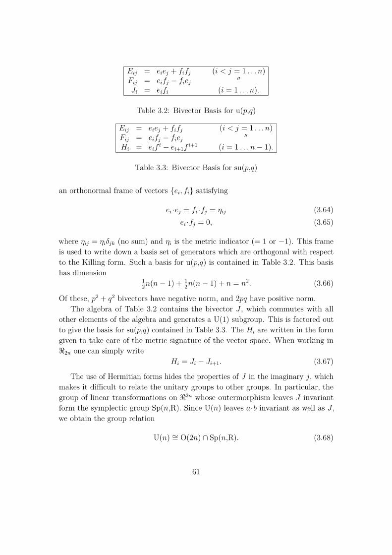
Eij = eiej + fifj (i < j = 1 . . . n)Fij = eifj − fiej ′′

Ji = eifi (i = 1 . . . n).

Table 3.2: Bivector Basis for u(p,q)

Eij = eiej + fifj (i < j = 1 . . . n)Fij = eifj − fiej ′′

Hi = eifi − ei+1f

i+1 (i = 1 . . . n− 1).

Table 3.3: Bivector Basis for su(p,q)

an orthonormal frame of vectors ei, fi satisfying

ei ·ej = fi ·fj = ηij (3.64)ei ·fj = 0, (3.65)

where ηij = ηiδjk (no sum) and ηi is the metric indicator (= 1 or −1). This frameis used to write down a basis set of generators which are orthogonal with respectto the Killing form. Such a basis for u(p,q) is contained in Table 3.2. This basishas dimension

12n(n− 1) + 1

2n(n− 1) + n = n2. (3.66)

Of these, p2 + q2 bivectors have negative norm, and 2pq have positive norm.The algebra of Table 3.2 contains the bivector J , which commutes with all

other elements of the algebra and generates a U(1) subgroup. This is factored outto give the basis for su(p,q) contained in Table 3.3. The Hi are written in the formgiven to take care of the metric signature of the vector space. When working in<2n one can simply write

Hi = Ji − Ji+1. (3.67)

The use of Hermitian forms hides the properties of J in the imaginary j, whichmakes it difficult to relate the unitary groups to other groups. In particular, thegroup of linear transformations on <2n whose outermorphism leaves J invariantform the symplectic group Sp(n,R). Since U(n) leaves a·b invariant as well as J ,we obtain the group relation

U(n) ∼= O(2n) ∩ Sp(n,R). (3.68)

61

More generally, we find that

U(p, q) ∼= O(2p, 2q) ∩ Sp(p, q,R), (3.69)

where Sp(p, q,R) is group of linear transformations leaving J invariant in themixed-signature space <2p,2q. The geometric algebra approach to Lie group theorymakes relations such as (3.69) quite transparent. Furthermore, the doublingbivector J appears in many other applications of geometric algebra — we saw oneoccurrence in Section 2.2.2 in the discussion of the Grassmann-Fourier transform.Other applications include multiparticle quantum mechanics and Hamiltonianmechanics [32]. Consistent use of geometric algebra can reveal these (often hidden)similarities between otherwise disparate fields.

3.3 The General Linear Group as a Spin GroupThe development of the general linear group as a spin group parallels that of theunitary groups. Again, the dimension of the space is doubled by introducing asecond space, but this time the second space has opposite signature. This leadsto the development of a Grassmann structure, as opposed to a complex structure.Vectors in <p,q are then replaced by null vectors in <n,n, where n = p+ q. Since a(positive) dilation of a null vector can also be given a rotor description, it becomespossible to build up a rotor description of the entire general linear group fromcombinations of dilations and orthogonal transformations.

The required construction is obtained by starting with a basis set of vectorsei in <p,q, and introducing a second space of opposite signature. The secondspace is generated by a set of vectors fi satisfying

ei ·ej = −fi ·fj (3.70)ei ·fj = 0, (3.71)

and the full set ei, fi form a basis set for <n,n. The vector space <n,n is split intotwo null spaces by introducing the bivector K defined by

K = ej∧fj = −ej∧f j. (3.72)

Again, K is independent of the initial choice of the ei frame. The bivector K

62

determines the linear function K by

K(a) ≡ a·K. (3.73)

The function K satisfies

K(ei) = fi K(fi) = eiK(ei) = −f i K(f i) = −ei, (3.74)

andK2(a) = (a·K)·K = a, (3.75)

for all vectors a.Proceeding as for the complexification bivector J we find that, for an arbitrary

bivector B,K(B) = −B + 1

2(B×K)×K. (3.76)

Any bivector commuting with K is therefore an eigenbivector of K, but now witheigenvalue −1.

An arbitrary vector a in <n,n can be decomposed into a pair of null vectors,

a = a+ + a−, (3.77)

where

a+ = 12(a+K(a)), (3.78)

a− = 12(a−K(a)). (3.79)

That a+ is null follows from

(a+)2 = 14

(a2 + 2a·(a·K) + (a·K)·(a·K)

)= 1

4(a2 − [(a·K)·K]·a)= 1

4(a2 − a2)= 0, (3.80)

and the same holds for a−. The scalar product between a+ and a− is, of course,non-zero:

a+ ·a− = 14(a2 − (a·K)2) = 1

2a2. (3.81)

This construction decomposes <n,n into two separate null spaces, Vn and Vn∗,

63

defined byK(a) = a ∀a ∈ VnK(a) = −a ∀a ∈ Vn∗, (3.82)

so that<n,n = Vn ⊕ Vn∗. (3.83)

A basis is defined for each of Vn and Vn∗ by

wi = 12(ei +K(ei)) (3.84)

w∗i = 12(ei −K(ei)), (3.85)

respectively. These basis vectors satisfy

wi ·wj = w∗i ·w∗j = 0 (3.86)

andw∗i ·wj = 1

2δij. (3.87)

In conventional accounts, the space Vn would be recognised as a Grassmannalgebra (all vector generators anticommute), with Vn∗ identified as the dual spaceof functions acting on Vn. In Chapter 2 we saw how both Vn and Vn∗ canbe represented in terms of functions in a single n-dimensional algebra. Here, adifferent construction is adopted in which the Vn and Vn∗ spaces are kept maximallydistinct, so that they generate a 2n-dimensional vector space. This is the moreuseful approach for the study of the Lie algebra of the general linear group. Weshall shortly see how these two separate approaches are reconciled by setting up anisomorphism between operations in the two algebras.

We are interested in the group of orthogonal transformations which keep theVn and Vn∗ spaces separate. For a vector a in Vn, the orthogonal transformationf must then satisfy

f(a) = f(a)·K. (3.88)

But, since a = a·K and f−1 = f , equation (3.88) leads to

a·K = f [f(a)·K]= a·f(K), (3.89)

64

Eij = eiej − eiej (i < j = 1 . . . n)Fij = eiej − eiej ′′

Ji = eiei (i = 1 . . . n).

Table 3.4: Bivector Basis for gl(n,R)

which must hold for all a. It follows that

f(K) = K (3.90)

and we will show that the f satisfying this requirement form the general lineargroup GL(n,R). The orthogonal transformations satisfying (3.90) can each be givena spin description, which enables the general linear group to be represented by aspin group. The elements of this spin group must satisfy

MK = KM. (3.91)

The generators of the rotor part of the spin group are therefore the set of bivectorswhich commute with K, which are eigenbivectors of K with eigenvalue −1.

Before writing down an orthogonal basis for the Lie algebra, it is useful tointroduce some further notation. We now take ei to be an orthonormal basisfor the Euclidean algebra <n, and ei to be the corresponding basis for theanti-Euclidean algebra <0,n. These basis vectors satisfy

ei ·ej = δij = −ei ·ejei ·ej = 0. (3.92)

The hat also serves as a convenient abbreviation for the action of K on a vector a,

a ≡ K(a). (3.93)

Since all bivectors in the Lie algebra of GL(n,R) are of the form B −K(B), anorthogonal basis for the Lie algebra can now be written down easily. Such a basisis contained in Table 3.4. The algebra in Table 3.4 includes K, which generates anabelian subgroup. This is factored out to leave the Lie algebra sl(n,R) containedin Table 3.5.

The form of the Lie algebra for the group GL(n,R) is clearly very close to thatfor U(n) contained in Table 3.2. The reason can be seen by considering the bilinear

65

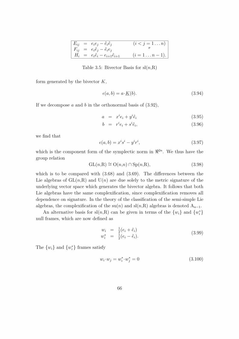
Eij = eiej − eiej (i < j = 1 . . . n)Fij = eiej − eiej ′′

Hi = eiei − ei+1ei+1 (i = 1 . . . n− 1).

Table 3.5: Bivector Basis for sl(n,R)

form generated by the bivector K,

ε(a, b) = a·K(b). (3.94)

If we decompose a and b in the orthonormal basis of (3.92),

a = xiei + yiei (3.95)b = riei + siei, (3.96)

we find thatε(a, b) = xisi − yiri, (3.97)

which is the component form of the symplectic norm in <2n. We thus have thegroup relation

GL(n,R) ∼= O(n,n) ∩ Sp(n,R), (3.98)

which is to be compared with (3.68) and (3.69). The differences between theLie algebras of GL(n,R) and U(n) are due solely to the metric signature of theunderlying vector space which generates the bivector algebra. It follows that bothLie algebras have the same complexification, since complexification removes alldependence on signature. In the theory of the classification of the semi-simple Liealgebras, the complexification of the su(n) and sl(n,R) algebras is denoted An−1.

An alternative basis for sl(n,R) can be given in terms of the wi and w∗i null frames, which are now defined as

wi = 12(ei + ei)

w∗i = 12(ei − ei).

(3.99)

The wi and w∗i frames satisfy

wi ·wj = w∗i ·w∗j = 0 (3.100)

66

andwiw

∗j + w∗jwi = δij, (3.101)

which are identifiable as the relations of the algebra of fermionic creation andannihilation operators. The pseudoscalars for the the Vn and Vn∗ spaces aredefined by

Wn = w1w2 . . . wnW ∗n = w∗1w

∗2 . . . w

∗n

(3.102)

respectively. If we now define

I+ij = 1

2(Eij + Fij)= 1

2(ei − ei)(ej + ej)= 2w∗iwj (3.103)

and

I−ij = 12(Eij − Fij)

= 12(ei + ei)(ej − ej)

= −2w∗jwi, (3.104)

we see that a complete basis for sl(n,R) is defined by the set I+ij , I

−ij , Hi. This

corresponds to the Chevalley basis for An−1. Furthermore, a complete basis set ofgenerators for GL(n,R) is given by the set w∗i ∧wj, defined over all i, j. This isperhaps the simplest of the possible basis sets for the Lie algebra, though it hasthe disadvantage that it is not orthogonal with respect to the Killing form.

We now turn to a proof that the subgroup of the spin group which leaves Kinvariant does indeed form a representation of GL(n,R). With a vector a in <nrepresented by the null vector a+ = (a+ a) in <n,n, we must prove that an arbitrarylinear transformation of a, a 7→ f(a), can be written in <n,n as

a+ 7→Ma+M−1, (3.105)

where M is a member of the spin group spin(n, n) which commutes with K. Westart by considering the polar decomposition of an arbitrary matrix M . Assumingthat det M 6= 0, the matrix MM can be written (not necessarliy uniquely) as

MM = SΛS (3.106)

67

where S is an orthogonal transformation (which can be arranged to be a rotationmatrix), and Λ is a diagonal matrix with positive entries. One can now write

M = SΛ1/2R (3.107)

where Λ1/2 is the diagonal matrix of positive square roots of the entries of Λ andR is a matrix defined by

R = Λ−1/2SM . (3.108)

The matrix R satisfies

RR = Λ−1/2SMMSΛ−1/2

= Λ−1/2ΛΛ−1/2

= I (3.109)

and so is also orthogonal. It follows from (3.107) that an arbitrary non-singularmatrix can be written as a diagonal matrix with positive entries sandwiched betweena pair of orthogonal matrices. As a check, this gives n2 degrees of freedom. Toprove the desired result, we need only show that orthogonal transformations andpositive dilations can be written in the form of equation (3.105).

We first consider rotations. The Eij generators in Table 3.4 produce rotors ofthe form

R = exp(E − E)/2, (3.110)

whereE = αijEij (3.111)

and the αij are a set of scalar coefficients. The effect of the rotor R on a+ generates

R(a+) = R(a+ a)R= RaR + (RaR)·K= eE/2ae−E/2 + (eE/2ae−E/2)·K (3.112)

and so accounts for all rotations of the vector a in <n. To complete the set oforthogonal transformations, a representation for reflections must be found as well.A reflection in the hyperplane orthogonal to the vector n in <n is represented bythe element nn in <n,n. Since nnnn = −1, nn is not a rotor and belongs to thedisconnected part of spin(n, n). That nn commutes with K, and so is contained in

68

spin(n, n), is verified as follows,

nnK = 2nn·K + nKn

= 2n2 + 2n·Kn+Knn

= 2(n2 + n2) +Knn

= Knn. (3.113)

The action of nn on a vector is determined by (3.8), and gives

nna+nn = −nnann− (nnann)·K= −nan− (nan)·K, (3.114)

as required.Finally, we need to see how positive dilations are given a rotor description. A

dilation in the n direction by an amount eλ is generated by the rotor

R = e−λnn/2, (3.115)

where the generator −λnn/2 is built from the Ki in Table 3.4. Acting on the nullvector n+ = n+ n, the rotor (3.115) gives

Rn+R = e−λnn/2n+e+λnn/2

= e−λnn(n+ n)= (cosh λ− nn sinh λ)(n+ n)= (cosh λ+ sinh λ)(n+ n)= eλn+. (3.116)

In addition, for vectors perpendicular to n in <n, the action of R on their nullvector equivalents has no effect. These are precisely the required properties for adilation in the n direction. This concludes the proof that the general linear groupis represented by the subgroup of spin(n, n) consisting of elements commutingwith K. As an aside, this construction has led us to the Eij and Ki generatorsin Table (3.4). Commutators of the Eij and Ki give the remaining Fij generators,which are sufficient to close the algebra.

The determinant of a linear function on <n is easily represented in <n,n since

f(e1)∧f(e2)∧. . .∧f(en) = det f En (3.117)

69

becomesMWnM

−1 = det fWn, (3.118)

in the null space of Vn. Here M is the spin group element representing the linearfunction f . From the definitions of Wn and W ∗

n (3.102), we can write

det f = 2n〈W ∗nMWnM

−1〉, (3.119)

from which many of the standard properties of determinants can be derived.

3.3.1 Endomorphisms of <nWe now turn to a second feature of <n,n, which is its effectiveness in discussingendomorphisms of <n. These are maps of <n onto itself, and the set of all such mapsis denoted end(<n). Since the algebra <n is 2n-dimensional, the endomorphismalgebra is isomorphic to the algebra of real 2n × 2n matrices,

end(<n) ∼= R(2n). (3.120)

But the Clifford algebra <n,n is also isomorphic to the algebra of 2n × 2n matrices,so every endomorphism of <n can be represented by a multivector in <n,n1. Ourfirst task is therefore to find how to construct each multivector equivalent of agiven endomorphism.

Within <n, endomorphisms are built up from the the primitive operations ofthe inner and outer products with the ei. It is more useful, however, to adoptthe following basis set of functions,

ei(A) ≡ ei ·A+ ei∧A = eiA (3.121)ei(A) ≡ −ei ·A+ ei∧A = Aei, (3.122)

where the hat (parity) operation in <n is defined by

Ar ≡ (−1)rAr (3.123)

and serves to distinguish even-grade and odd-grade multivectors. The reason forthe use of the hat in both <n and <n,n will become apparent shortly. The ei andei operations are precisely those found in Section 2.3 in the context of Berezin

1I am grateful to Frank Sommen and Nadine Van Acker for pointing out the potential usefulnessof this result.

70

calculus, though with the fiducial tensor h now set to the identity. They satisfythe relations

eiej + ejei = 2δijeiej + ej ei = −2δij (3.124)eiej + ejei = 0, (3.125)

which are the defining relations for a vector basis in <n,n. This establishes theisomorphism between elements of end(<n) and multivectors in <n,n. Any element ofend(<n) can be decomposed into sums and products of the ei and ei functions,and so immediately specifies a multivector in <n,n built from the same combinationsof the ei and ei basis vectors.

To complete the construction, we must find a 2n-dimensional subspace of <n,non which endomorphisms of <n are faithfully represented by (left) multiplicationby elements of <n,n. The required subspace is a minimal left ideal of <n,n and isdenoted In. It is constructed as follows. We define a set of bivector blades by

Ki ≡ eiei. (3.126)

Here, and in the remainder of this section, we have dropped the summationconvention. The Ki satisfy

Ki ·Kj = δij (3.127)Ki×Kj = 0 (3.128)

and the bivector K is can be written as

K =∑i

Ki. (3.129)

A family of commuting idempotents are now defined by

Ii ≡ 12(1 +Ki) = w∗iwi, (3.130)

71

and have the following properties:

I2i = Ii (3.131)

IiIj = IjIi (3.132)eiIi = wi = eiIi (3.133)Iiei = w∗i = −Iiei (3.134)

KiIi = Ii. (3.135)

From the Ii the idempotent I is defined by

I ≡n∏i=1

Ii = I1I2 . . . In = w∗1w1w∗2w2 . . . w

∗nwn = W ∗

nWn. (3.136)

I has the following properties:

I2 = I (3.137)eiI = eiI (3.138)

andEnI = EnI = WnI = Wn, (3.139)

where En is the pseudoscalar for the Euclidean algebra <n and En is the pseudoscalarfor the anti-Euclidean algebra <0,n. The relationships in (3.139) establish anequivalence between the <n, <0,n and Vn vector spaces.

Whilst the construction of I has made use of an orthonormal frame, the form ofI is actually independent of this choice. This can be seen by writing I in the form

I = 12n(

1 +K + K∧K2! + . . .+ K∧K∧. . .∧K

n!

)(3.140)

and recalling that K is frame-independent. It is interesting to note that thebracketed term in (3.140) is of the same form as the Grassmann exponentialconsidered in Section 2.2.1.

The full 2n-dimensional space In is generated by left multiplication of I by theentire algebra <n,n,

In = <n,nI. (3.141)

Since multiplication of I by ei and ei are equivalent, every occurrence of an ei ina multivector in <n,n can be replaced by an ei, so that there is a simple 1 ↔ 1

72

equivalence between elements of <n and In. The action of an element of end(<n)can now be represented in <n,n by left multiplication of In by the appropriatemultivector. For a multivector Ar in <n the equivalence between the basic operators(3.122) is seen from

eiArI ↔ eiAr (3.142)

andeiArI ↔ Arei. (3.143)

The parity operation on the right-hand side of (3.143) arises because the ei vectormust be anticommuted through each of the vectors making up the Ar multivector.This is the reason for the different uses of the overhat notation for the <n and <n,nalgebras. Symbolically, we can now write

eiIn ↔ ei<n (3.144)eiIn ↔ <nei. (3.145)

Also, from the definitions of wi and w∗i (3.99), we find the equivalences

wiIn ↔ ei∧<n (3.146)w∗i In ↔ ei ·<n, (3.147)

which establishes contact with the formalism of Grassmann/Berezin calculus givenin Chapter 2. We can now move easily between the formalism with dot and wedgeproducts used in Chapter 2 and the null-vector formalism adopted here. The chosenapplication should dictate which is the more useful.

We next consider the quantity nn, where n is a unit vector. The action of thison In gives

nnIn ↔ n<nn. (3.148)

The operation on the right-hand side is the outermorphism action of a reflection inthe hyperplane perpendicular to n. In the previous section we used a double-sidedapplication of nn on null vectors to represent reflections in <n. We now see that thesame object can be applied single-sidedly in conjunction with the idempotent I toalso produce reflections. The same is true of products of reflections. For example,the rotor (3.110) gives

e(E−E)/2MI = eE/2Me−E/2I ↔ eE/2Me−E/2, (3.149)

73

demonstrating how the two-bladed structure of the Eij generators is used torepresent concurrent left and right multiplication in <n.

The operation <n 7→ <n is performed by successive reflections in each of the eidirections. We therefore find the equivalence

e1e1e2e2 . . . enenIn ↔ <n. (3.150)

Bute1e1e2e2 . . . enen = en . . . e2e1e1e2 . . . en = EnEn = En,n (3.151)

is the unit pseudoscalar in <n,n, so multiplication of an element of In by En,ncorresponds to the parity operation in <n. As a check, (En,n)2 is always +1, so theresult of two parity operations is always the identity.

The correspondence between the single-sided and double-sided forms for adilation are not quite so simple. If we consider the rotor exp−λnn/2 again, wefind that, for the vector n,

e−λnn/2nI = eλ/2nI ↔ eλ/2n (3.152)

For vectors perpendicular to n, however, we find that

e−λnn/2n⊥I = n⊥e−λ/2nnI ↔ e−λ/2n⊥, (3.153)

so the single-sided formulation gives a stretch along the n direction of expλ, butnow combined with an overall dilation of exp−λ/2. This overall factor can beremoved by an additional boost with the exponential of a suitable multiple of K.It is clear, however, that both single-sided and double-sided application of elementsof the spin group which commute with K can be used to give representations ofthe general linear group.

Finally, we consider even products of the null vectors wi and w∗i . These generatethe operations

wiw∗i In ↔ ei ·(ei∧<n)

w∗iwiIn ↔ ei∧(ei ·<n) (3.154)

which are rejection and projection operations in <n respectively. For a vector a in<n, the operation of projecting a onto the ei direction is performed by

Pi(a) = eiei ·a, (3.155)

74

and for a general multivector,

Pi(A) = ei∧(ei ·A). (3.156)

This projects out the components of A which contain a vector in the ei direction.The projection onto the orthogonal complement of ei (the rejection) is given by

P⊥i (A) = ei ·(ei∧A). (3.157)

Projection operations correspond to singular transformations, and we now see thatthese are represented by products of null multivectors in <n,n. This is sufficient toensure that singular transformations can also be represented by an even product ofvectors, some of which may now be null.

Two results follow from these considerations. Firstly, every matrix Lie groupcan be represented by a spin group — every matrix Lie group can be defined as asubgroup of GL(n,R) and we have shown how GL(n,R) can be represented as a spingroup. It follows that every Lie algebra can be represented by a bivector algebra,since all Lie algebras have a matrix representation via the adjoint representation.The discussion of the unitary group has shown, however, that subgroups of GL(n,R)are not, in general, the best way to construct spin-group representations. Other,more useful, constructions are given in the following Sections. Secondly, everylinear transformation on <n can be represented in <n,n as an even product ofvectors, the result of which commutes with K. It is well known that quaternionsare better suited to rotations in three dimensions than 3× 3 matrices. It shouldnow be possible to extend these advantages to arbitrary linear functions. A numberof other applications for these results can be envisaged. For example, consider theequation

u′(s) = M (s)u(s), (3.158)

where u(s) and M (s) are vector and matrix functions of the parameter s and theprime denotes the derivative with respect to s. By replacing the vector u by thenull vector u in <n,n, equation (3.158) can be written in the form

u′ = B(s)·u, (3.159)

where B(s) is a bivector. If we now write u = Ru0R, where u0 is a constant vector,then equation (3.158) reduces to the rotor equation

R′ = 12BR, (3.160)

75

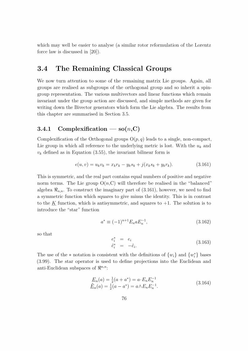
which may well be easier to analyse (a similar rotor reformulation of the Lorentzforce law is discussed in [20]).

3.4 The Remaining Classical GroupsWe now turn attention to some of the remaining matrix Lie groups. Again, allgroups are realised as subgroups of the orthogonal group and so inherit a spin-group representation. The various multivectors and linear functions which remaininvariant under the group action are discussed, and simple methods are given forwriting down the Bivector generators which form the Lie algebra. The results fromthis chapter are summarised in Section 3.5.

3.4.1 Complexification — so(n,C)Complexification of the Orthogonal groups O(p, q) leads to a single, non-compact,Lie group in which all reference to the underlying metric is lost. With the uk andvk defined as in Equation (3.55), the invariant bilinear form is

ε(u, v) = ukvk = xkrk − yksk + j(xksk + ykrk). (3.161)

This is symmetric, and the real part contains equal numbers of positive and negativenorm terms. The Lie group O(n,C) will therefore be realised in the “balanced”algebra <n,n. To construct the imaginary part of (3.161), however, we need to finda symmetric function which squares to give minus the identity. This is in contrastto the K function, which is antisymmetric, and squares to +1. The solution is tointroduce the “star” function

a∗ ≡ (−1)n+1EnaE−1n , (3.162)

so thate∗i = eie∗i = −ei.

(3.163)

The use of the ∗ notation is consistent with the definitions of wi and w∗i bases(3.99). The star operator is used to define projections into the Euclidean andanti-Euclidean subspaces of <n,n:

En(a) = 12(a+ a∗) = a·EnE−1

n

En(a) = 12(a− a∗) = a∧EnE−1

n .(3.164)

76

Eij = eiej − eiej (i < j = 1 . . . n)Fij = eiej + eiej.

′′

Table 3.6: Bivector Basis for so(n,C)

The Euclidean pseudoscalar En anticommutes with K, so the star operator anti-commutes with the K function. It follows that the combined function

K∗(a) ≡ K(a∗) (3.165)

satisfies

K∗2(a) = K[K(a∗)∗]= −K[K(a∗∗)]= −a (3.166)

and

K∗(a) = −[K(a)]∗

= K∗(a), (3.167)

and so has the required properties. The complex symmetric norm can now bewritten on <n,n as

ε(a, b) = a·b+ ja·K∗(b), (3.168)

which can verified by expanding in the ei, ei basis of (3.92).An orthogonal transformation f will leave ε(a, b) invariant provided that

K∗f(a) = f K∗(a), (3.169)

which defines the group O(n,C). Each function f in O(n,C) can be constructedfrom the corresponding elements of spin(n, n), which defines the spin-group repre-sentation. The bivector generators must satisfy

K∗[eλB/2ae−λB/2] = eλB/2K∗(a)e−λB/2, (3.170)

77

which reduces to the requirement

K∗(B ·a) = B ·K∗(a) (3.171)⇒ B ·a = −K∗[B ·K∗(a)] = −K∗(B)·a (3.172)⇒ K∗(B) = −B. (3.173)

Since K∗2(B) = B for all bivectors B, the generators which form the Lie algebraso(n,C) are all of the form B−K∗(B). This is used to write down the bivector basisin Table 3.6. Under the commutator product, the Eij form a closed sub-algebrawhich is isomorphic to so(n). The Fij fulfil the role of “jEij”. The Killing metrichas n(n− 1)/2 entries of positive and signature and the same number of negativesignature.

3.4.2 Quaternionic Structures — sp(n) and so∗(2n)The quaternionic unitary group (usually denoted Sp(n) or HU(n)) is the invariancegroup of the Hermitian-symmetric inner product of quaternion-valued vectors. Byanalogy with the unitary group, the quaternionic structure is introduced by nowquadrupling the real space <n or <p,q to <4n or <4p,4q. We deal with the Euclideancase first and take ei to be an orthonormal basis set for <n. Three further copiesof <n are introduced, so that ei, e1

i , e2i , e

3i form an orthonormal basis for <4n.

Three “doubling” bivectors are now defined as

J1 = eie1i + e2

i e3i

J2 = eie2i + e3

i e1i

J3 = eie3i + e1

i e2i ,

(3.174)

which define the three functions

J i(a) = a·Ji. (3.175)

(The introduction of an orthonormal frame is not essential since each of the Jiare independent of the intial choice of frame. Orthonormal frames do ease thediscussion of the properties of the Ji, however, so will be used frequently in thisand the following sections).

78

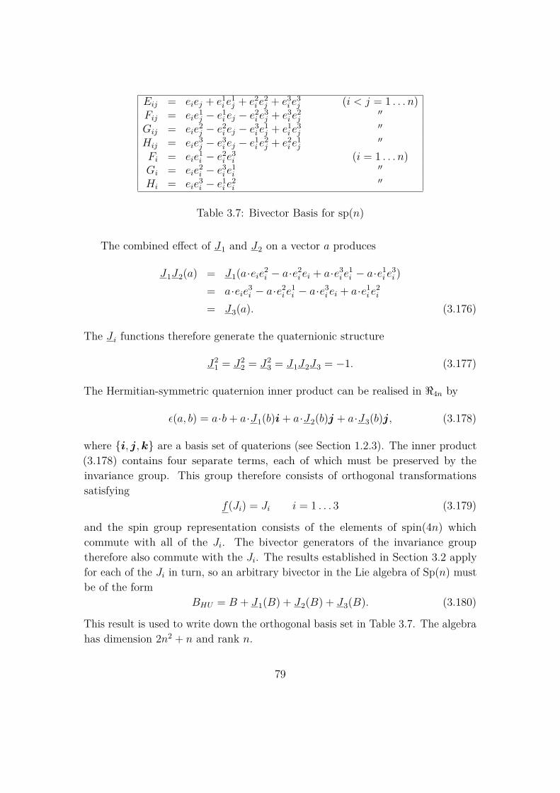
Eij = eiej + e1i e

1j + e2

i e2j + e3

i e3j (i < j = 1 . . . n)

Fij = eie1j − e1

i ej − e2i e

3j + e3

i e2j

′′

Gij = eie2j − e2

i ej − e3i e

1j + e1

i e3j

′′

Hij = eie3j − e3

i ej − e1i e

2j + e2

i e1j

′′

Fi = eie1i − e2

i e3i (i = 1 . . . n)

Gi = eie2i − e3

i e1i

′′

Hi = eie3i − e1

i e2i

′′

Table 3.7: Bivector Basis for sp(n)

The combined effect of J1 and J2 on a vector a produces

J1J2(a) = J1(a·eie2i − a·e2

i ei + a·e3i e

1i − a·e1

i e3i )

= a·eie3i − a·e2

i e1i − a·e3

i ei + a·e1i e

2i

= J3(a). (3.176)

The J i functions therefore generate the quaternionic structure

J21 = J2

2 = J23 = J1J2J3 = −1. (3.177)

The Hermitian-symmetric quaternion inner product can be realised in <4n by

ε(a, b) = a·b+ a·J1(b)i + a·J2(b)j + a·J3(b)j, (3.178)

where i, j,k are a basis set of quaterions (see Section 1.2.3). The inner product(3.178) contains four separate terms, each of which must be preserved by theinvariance group. This group therefore consists of orthogonal transformationssatisfying

f(Ji) = Ji i = 1 . . . 3 (3.179)

and the spin group representation consists of the elements of spin(4n) whichcommute with all of the Ji. The bivector generators of the invariance grouptherefore also commute with the Ji. The results established in Section 3.2 applyfor each of the Ji in turn, so an arbitrary bivector in the Lie algebra of Sp(n) mustbe of the form

BHU = B + J1(B) + J2(B) + J3(B). (3.180)

This result is used to write down the orthogonal basis set in Table 3.7. The algebrahas dimension 2n2 + n and rank n.

79

The above extends easily to the case of sp(p, q) by working in the algebra <4p,4q.With ei now a basis for <p,q, the doubling bivectors are defined by

J1 = eie1i + e2

i e3i etc (3.181)

and the quaternion relations (3.177) are still satisfied. The Lie algebra is thengenerated in exactly the same may. The resultant algebra has a Killing metric with2(p2 + q2) + p+ q negative entries and 4pq positive entries.

The properties of the K∗ function found in Section 3.4.1 suggests that analternative quaternionic structure could be found in <2n,2n by introducing anti-commuting K∗ and J functions. This is indeed the case. With ei and fi apair of anticommuting orthonormal bases for <n, a basis for <2n,2n is defined byei, fi, ei, fi. The hat operation is now defined by

a = K(a) = a·K (3.182)

withK = eiei + fifi. (3.183)

A complexification bivector is defined by

J = eifi + eif

i = eifi − eifi (3.184)

and additional doubling bivectors are defined by

K1 = eiei − fifiK1 = eifi + fiei.

(3.185)

The set J,K1, K2 form a set of three bivectors, no two of which commute.With pseudoscalars En and Fn defined by

En = e1e2 . . . enFn = f1f2 . . . fn,

(3.186)

the star operation is defined by

a∗ = −EnFnaFnEn. (3.187)

80

K∗i operations are now defined by

K∗i (a) = Ki(a∗) = a∗ ·Ki. (3.188)

These satisfyK∗i

2(a) = −a (3.189)

and

K∗1K∗2(a) = K1[K2(a∗)∗]

= −K1K2(a)= J(a). (3.190)

The J and K∗i therefore form a quaternionic set of linear functions satisfying

K∗12 = K∗2

2 = J2 = K∗1K∗2J = −1. (3.191)

Orthogonal functions commuting with each of the J and K∗i functions will thereforeleave a quaternionic inner product invariant. This inner product can be written as

ε(a, b) = a·J(b) + ia·b+ ja·K∗1(b) + ka·K∗2(b), (3.192)

which expansion in the ei, fi, ei, fi frame shows to be equivalent to the skew-Hermitian quaternionic inner product

ε(u, v) = u†kivk. (3.193)

The invariance group of (3.193) is denoted SO∗(2n) (or Sk(n,H)). The bivectorgenerators of the invariance group must satisfy J(B) = B and K∗i (B) = −B andso are of the form

BH∗ = B + J(B)−K∗1(B)−K∗2(B). (3.194)

This leads to the orthogonal set of basis generators in Table 3.8.The bivector algebra so∗(n) has dimension n(2n− 1) and a Killing metric with

n2 negative entries and n2 − n positive entries. This algebra is one of the possiblereal forms of the complexified algebra Dn. Some of the properties of so∗(2n),including its representation theory, have been discussed by Barut & Bracken [58].

81

Eij = eiej + fifj − eiej − fifj (i < j = 1 . . . n)Fij = eifj − fiej + eifj − fiej ′′

Gij = eiej + eiej + fifj + fifj′′

Hij = eifj + fiej − fiej − eifj ′′

Hi = eifi + eifi (i = 1 . . . n)

Table 3.8: Bivector Basis for so∗(n)

3.4.3 The Complex and Quaternionic General LinearGroups

The general linear group over the complex field, GL(n,C), is constructed fromlinear functions in the 2n-dimensional space <2n which leave the complex structureintact,

h(a)·J = h(a·J). (3.195)

These linear functions can be represented by orthogonal functions in <2n,2n using thetechniques introduced in Section 3.3. Thus, using the conventions of Section 3.4.2,a vector a in <2n is represented in <2n,2n by the null vector a+ = a + a, and thecomplex structure is defined by the bivector J of equation (3.184). These definitionsensure that the J function keeps null vectors in the same null space,

K J(a) = J K(a) (3.196)

⇒ (a·J)·K − (a·K)·J = a·(J×K) = 0, (3.197)

which is satisfied since J×K = 0. The spin group representation of GL(n,C)consists of all elements of spin(2n, 2n) which commute with both J and K andhence preserve both the null and complex structures. The bivector generators ofthe Lie algebra gl(n,C) are therefore of the form

BC = B + J(B)−K(B)−K J(B) (3.198)

which yields the set of generators in Table 3.9. This algebra has 2n2 generators, asis to be expected. The two abelian subgroups are removed in the usual mannerto yield the Lie algebra for sl(n,C) given in Table 3.10. The Killing metric givesn2 − 1 terms of both positive and negative norm.

The general linear group with quaternionic entries (denoted U∗(2n) or GL(n,H))is constructed in the same manner as the above, except that now the group is

82

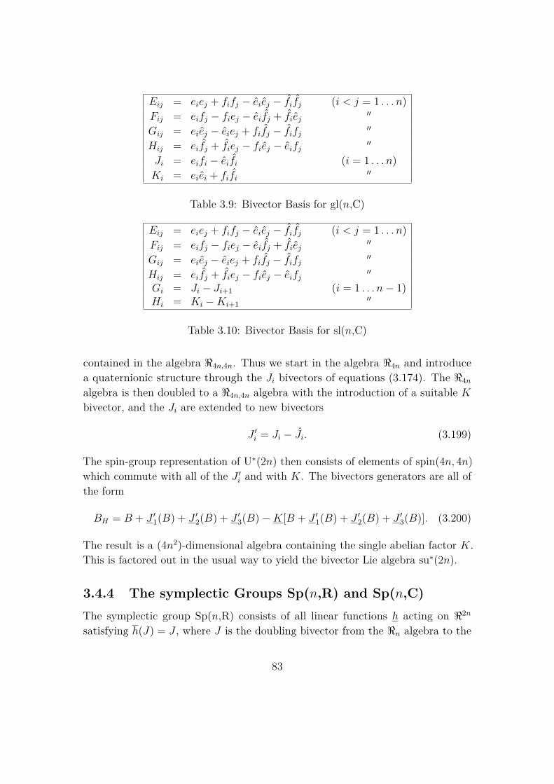
Eij = eiej + fifj − eiej − fifj (i < j = 1 . . . n)Fij = eifj − fiej − eifj + fiej

′′

Gij = eiej − eiej + fifj − fifj ′′

Hij = eifj + fiej − fiej − eifj ′′

Ji = eifi − eifi (i = 1 . . . n)Ki = eiei + fifi

′′

Table 3.9: Bivector Basis for gl(n,C)

Eij = eiej + fifj − eiej − fifj (i < j = 1 . . . n)Fij = eifj − fiej − eifj + fiej

′′

Gij = eiej − eiej + fifj − fifj ′′

Hij = eifj + fiej − fiej − eifj ′′

Gi = Ji − Ji+1 (i = 1 . . . n− 1)Hi = Ki −Ki+1

′′

Table 3.10: Bivector Basis for sl(n,C)

contained in the algebra <4n,4n. Thus we start in the algebra <4n and introducea quaternionic structure through the Ji bivectors of equations (3.174). The <4n

algebra is then doubled to a <4n,4n algebra with the introduction of a suitable Kbivector, and the Ji are extended to new bivectors

J ′i = Ji − Ji. (3.199)

The spin-group representation of U∗(2n) then consists of elements of spin(4n, 4n)which commute with all of the J ′i and with K. The bivectors generators are all ofthe form

BH = B + J ′1(B) + J ′2(B) + J ′3(B)−K[B + J ′1(B) + J ′2(B) + J ′3(B)]. (3.200)

The result is a (4n2)-dimensional algebra containing the single abelian factor K.This is factored out in the usual way to yield the bivector Lie algebra su∗(2n).

3.4.4 The symplectic Groups Sp(n,R) and Sp(n,C)The symplectic group Sp(n,R) consists of all linear functions h acting on <2n

satisfying h(J) = J , where J is the doubling bivector from the <n algebra to the

83

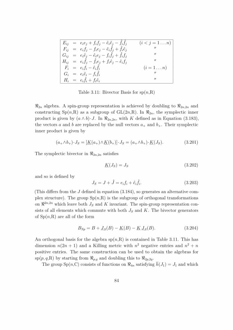
Eij = eiej + fifj − eiej − fifj (i < j = 1 . . . n)Fij = eifj − fiej − eifj + fiej

′′

Gij = eiej − eiej − fifj + fifj′′

Hij = eifj − fiej + fiej − eifj ′′

Fi = eifi − eifi (i = 1 . . . n)Gi = eiei − fifi ′′

Hi = eifi + fiei′′

Table 3.11: Bivector Basis for sp(n,R)

<2n algebra. A spin-group representation is achieved by doubling to <2n,2n andconstructing Sp(n,R) as a subgroup of GL(2n,R). In <2n, the symplectic innerproduct is given by (a ∧ b)·J . In <2n,2n, with K defined as in Equation (3.183),the vectors a and b are replaced by the null vectors a+ and b+. Their symplecticinner product is given by

(a+∧b+)·JS = [K(a+)∧K(b+)]·JS = (a+∧b+)·K(JS). (3.201)

The symplectic bivector in <2n,2n satisfies

K(JS) = JS (3.202)

and so is defined byJS = J + J = eifi + eifi. (3.203)

(This differs from the J defined in equation (3.184), so generates an alternative com-plex structure). The group Sp(n,R) is the subgroup of orthogonal transformationson <2n,2n which leave both JS and K invariant. The spin-group representation con-sists of all elements which commute with both JS and K. The bivector generatorsof Sp(n,R) are all of the form

BSp = B + JS(B)−K(B)−K JS(B). (3.204)

An orthogonal basis for the algebra sp(n,R) is contained in Table 3.11. This hasdimension n(2n + 1) and a Killing metric with n2 negative entries and n2 + n

positive entries. The same construction can be used to obtain the algebras forsp(p, q,R) by starting from <p,q and doubling this to <2p,2q.

The group Sp(n,C) consists of functions on <4n satisfying h(J1) = J1 and which

84

also preserve the complex structure,

h(a·J3) = h(a)·J3. (3.205)

The complex and symplectic structures satisfy J3(J1) = −J1, so J3 and J1 donot commute. Instead they are two-thirds of the quaternionic set of bivectorsintroduced in Section 3.4.2. The C-skew inner product on <4n is written

ε(a, b) = a·J1(b)− ja·J1J3(b) = a·J1(b) + ja·J2(b). (3.206)

By analogy with Sp(n,R), a spin-group representation of Sp(n,C) is constructedas a subgroup of GL(2n,C)in <4n,4n. With the null structure defined by K, thesymplectic structure is now determined by

JS = J1 +K(J1) (3.207)

and the complex structure by

J = J2 −K(J). (3.208)

The Lie algebra sp(n,C) is formed from the set of bivectors in <24n,4n which commute

with all of the K, J and JS bivectors. With this information, it is a simple matterto write down a basis set of generators.

3.5 SummaryIn the preceding sections we have seen how many matrix Lie groups can berepresented as spin groups, and how all (finite dimensional) Lie algebras can berealised as bivector algebras. These results are summarised in Tables 3.12 and 3.13.Table 3.12 lists the classical bilinear forms, their invariance groups, the base spacein which the spin group representation is constructed and the general form of thebivector generators. The remaining general linear groups are listed in Table 3.13.Again, their invariant bivectors and the general form of the generators are listed.For both tables, the conventions for the various functions and bivectors used arethose of the section where the group was discussed.

A number of extensions to this work can be considered. It is well known, forexample, that the Lie group G2 can be constructed in <0,7 as the invariance groupof a particular trivector (which is given in [46]). This suggests that the techniques

85

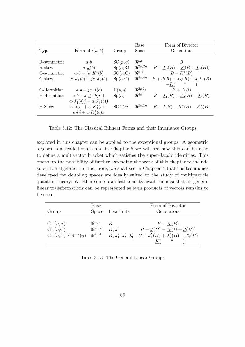
Base Form of BivectorType Form of ε(a, b) Group Space Generators

R-symmetric a·b SO(p, q) <p,q BR-skew a·J(b) Sp(n,R) <2n,2n B + JS(B)−K(B + JS(B))C-symmetric a·b+ ja·K∗(b) SO(n,C) <n,n B −K∗(B)C-skew a·J1(b) + ja·J2(b) Sp(n,C) <4n,4n B + J(B) + JS(B) + J JS(B)

−K( ′′ )C-Hermitian a·b+ ja·J(b) U(p, q) <2p,2q B + J(B)H-Hermitian a·b+ a·J1(b)i + Sp(n) <4n B + J1(B) + J2(B) + J3(B)

a·J2(b)j + a·J3(b)jH-Skew a·J(b) + a·K∗1(b)+ SO∗(2n) <2n,2n B + J(B)−K∗1(B)−K∗2(B)

a·bi + a·K∗2(b)k

Table 3.12: The Classical Bilinear Forms and their Invariance Groups

explored in this chapter can be applied to the exceptional groups. A geometricalgebra is a graded space and in Chapter 5 we will see how this can be usedto define a multivector bracket which satisfies the super-Jacobi identities. Thisopens up the possibility of further extending the work of this chapter to includesuper-Lie algebras. Furthermore, we shall see in Chapter 4 that the techniquesdeveloped for doubling spaces are ideally suited to the study of multiparticlequantum theory. Whether some practical benefits await the idea that all generallinear transformations can be represented as even products of vectors remains tobe seen.

Base Form of BivectorGroup Space Invariants Generators

GL(n,R) <n,n K B −K(B)GL(n,C) <2n,2n K, J B + J(B)−K(B + J(B))GL(n,H) / SU∗(n) <4n,4n K, J ′1, J

′2, J

′3 B + J ′1(B) + J ′2(B) + J ′3(B)

−K( ′′ )

Table 3.13: The General Linear Groups

86

Chapter 4

Spinor Algebra

This chapter describes a translation between conventional matrix-based spinoralgebra in three and four dimensions [59, 60], and an approach based entirely inthe (real) geometric algebra of spacetime. The geometric algebra of Minkowskispacetime is called the spacetime algebra or, more simply, the STA. The STA wasintroduced in Section 1.2.5 as the geometric algebra generated by a set of fourorthonormal vectors γµ, µ = 0 . . . 3, satisfying

γµ ·γν = ηµν = diag(+ − − −). (4.1)

Whilst the γµ satisfy the Dirac algebra generating relations, they are to bethought of as an orthonormal frame of independent vectors and not as componentsof a single “isospace” vector. The full STA is spanned by the basis

1, γµ σk, iσk, iγµ, i, (4.2)

wherei ≡ γ0γ1γ2γ3 (4.3)

andσk ≡ γkγ0. (4.4)

The meaning of these equation was discussed in Section 1.2.5.The aim of this chapter is to express both spinors and matrix operators within

the real STA. This results in a very powerful language in which all algebraicmanipulations can be performed without ever introducing a matrix representation.The Pauli matrix algebra is studied first, and an extension to multiparticle systemsis introduced. The Dirac algebra and Dirac spinors are then considered. The

87

translation into the STA quickly yields the Dirac equation in the form first foundby Hestenes [17, 19, 21, 27]. The concept of the multiparticle STA is introduced,and is used to formulate a number of two-particle relativistic wave equations. Someproblems with these are discussed and a new equation, which has no spinorialcounterpart, is proposed. The chapter concludes with a discussion of the 2-spinorcalculus of Penrose & Rindler [36]. Again, it is shown how a scalar unit imaginaryis eliminated by the use of the real multiparticle STA. Some sections of this chapterappeared in the papers “States and operators in the spacetime algebra” [6] and“2-Spinors, twistors and supersymmetry in the spacetime algebra [4].

4.1 Pauli SpinorsThis section establishes a framework for the study of the Pauli operator algebra andPauli spinors within the geometric algebra of 3-dimensional space. The geometricalgebra of space was introduced in Section 1.2.3 and is spanned by

1, σk, iσk, i. (4.5)

Here the σk are a set of three relative vectors (spacetime bivectors) in theγ0-system. Vectors in this system are written in bold type to distinguish themfrom spacetime vectors. There is no possible confusion with the σk symbols, sothese are left in normal type. When working non-relativistically within the evensubalgebra of the full STA some notational modifications are necessary. Relativevectors σk and relative bivectors iσk are both bivectors in the full STA, sospatial reversion and spacetime reversion have different effects. To distinguishthese, we define the operation

A† = γ0Aγ0, (4.6)

which defines reversion in the Pauli algebra. The presence of the γ0 vector in thedefinition of Pauli reversion shows that this operation is dependent on the choiceof spacetime frame. The dot and wedge symbols also carry different meaningsdependent on whether their arguments are treated as spatial vectors or spacetimebivectors. The convention adopted here is that the meaning is determined bywhether their arguments are written in bold type or not. Bold-type objects aretreated as three-dimensional multivectors, whereas normal-type objects are treatedas belonging to the full STA. This is the one potentially confusing aspect ofour conventions, though in practice the meaning of all the symbols used is quite

88

unambiguous.The Pauli operator algebra [59] is generated by the 2× 2 matrices

σ1 =(

0 11 0

), σ2 =

(0 −jj 0

), σ3 =

(1 00 −1

). (4.7)

These operators act on 2-component complex spinors

|ψ〉 =(ψ1

ψ2

), (4.8)

where ψ1 and ψ2 are complex numbers. We have adopted a convention by whichstandard quantum operators appear with carets, and quantum states are writtenas kets and bras. We continue to write the unit scalar imaginary of conventionalquantum mechanics as j, which distinguishes it from the geometric pseudoscalar i.

To realise the Pauli operator algebra within the algebra of space, the columnPauli spinor |ψ〉 is placed in one-to-one correspondence with the even multivectorψ (which satisfies ψ = γ0ψγ0) through the identification1

|ψ〉 =(

a0 + ja3

−a2 + ja1

)↔ ψ = a0 + akiσk. (4.9)

In particular, the basis spin-up and spin-down states become(10

)↔ 1 (4.10)

and (01

)↔ −iσ2. (4.11)

The action of the four quantum operators σk, j can now be replaced by theoperations

σk |ψ〉 ↔ σkψσ3 (k = 1, 2, 3) (4.12)

andj |ψ〉 ↔ ψiσ3. (4.13)

1This mapping was first found by Anthony Lasenby.

89

Verifying these relations is a matter of routine computation, for example

σ1 |ψ〉 =(−a2 + ja1

a0 + ja3

)↔ −a2 + a1iσ3

−a0iσ2 + a3iσ1= σ1

(a0 + akiσk

)σ3. (4.14)

With these definitions, the action of complex conjugation of a Pauli spinor translatesto

|ψ〉∗ ↔ σ2ψσ2. (4.15)

The presence of a fixed spatial vector on the left-hand side of ψ shows that complexconjugation is a frame-dependent concept.

As an illustration, the Pauli equation (in natural units),

j∂t |ψ〉 = 12m

((−j∇− eA)2 − eσkBk

)|ψ〉+ eV |ψ〉 , (4.16)

can be written (in the Coulomb gauge) as [22]

∂tψiσ3 = 12m(−∇2ψ + 2eA·∇ψiσ3 + e2A2ψ)− e

2mBψσ3 + eV ψ, (4.17)

where B is the magnetic field vector Bkσk. This translation achieves two importantgoals. The scalar unit imaginary is eliminated in favour of right-multiplicationby iσ3, and all terms (both operators and states) are now real-space multivectors.Removal of the distinction between states and operators is an important conceptualsimplification.

We next need to find a geometric algebra equivalent of the spinor inner product〈ψ |φ〉. In order to see how to handle this, we need only consider its real part. Thisis given by

<〈ψ |φ〉 ↔ 〈ψ†φ〉, (4.18)

so that, for example,

〈ψ |ψ〉 ↔ 〈ψ†ψ〉 = 〈(a0 − iajσj)(a0 + iakσk)〉= (a0)2 + akak. (4.19)

Since〈ψ|φ〉 = <〈ψ|φ〉 − j<〈ψ|jφ〉, (4.20)

90

the full inner product becomes

〈ψ |φ〉 ↔ (ψ, φ)S ≡ 〈ψ†φ〉 − 〈ψ†φiσ3〉iσ3. (4.21)

The right hand side projects out the 1, iσ3 components from the geometricproduct ψ†φ. The result of this projection on a multivector A is written 〈A〉S. ForPauli-even multivectors this projection has the simple form

〈A〉S = 12(A− iσ3Aiσ3). (4.22)

As an example of (4.21), consider the expectation value

〈ψ|σk |ψ〉 ↔ 〈ψ†σkψσ3〉 − 〈ψ†σkψi〉iσ3 = σk ·〈ψσ3ψ†〉1, (4.23)

which gives the mean value of spin measurements in the k direction. The STAform indicates that this is the component of the spin vector s = ψσ3ψ

† in the σkdirection, so that s is the coordinate-free form of this vector. Since ψσ3ψ

† is bothPauli-odd and Hermitian-symmetric (reverse-symmetric in the Pauli algebra), s

contains only a vector part. (In fact, both spin and angular momentum are betterviewed as bivector quantities, so it is usually more convenient to work with is

instead of s.)Under an active rotation, the spinor ψ transforms as

ψ 7→ ψ′ = R0ψ, (4.24)

where R0 is a constant rotor. The quantity ψ′ is even, and so is a second spinor.(The term “spinor” is used in this chapter to denote any member of a linearspace which is closed under left-multiplication by a rotor R0.) The correspondingtransformation law for s is

s 7→ s′ = R0sR†0, (4.25)

which is the standard double-sided rotor description for a rotation, introduced inSection 1.2.4.

The definitions (4.9), (4.12) and (4.13) have established a simple translationfrom the language of Pauli operators and spinors into the geometric algebra ofspace. But the STA formulation can be taken further to afford new insights intothe role of spinors in the Pauli theory. By defining

ρ = ψψ† (4.26)

91

the spinor ψ can be writtenψ = ρ1/2R, (4.27)

where R is defined asR = ρ−1/2ψ. (4.28)

R satisfiesRR† = 1 (4.29)

and is therefore a spatial rotor. The spin vector can now be written

s = ρRσ3R†, (4.30)

which demonstrates that the double-sided construction of the expectation value(4.23) contains an instruction to rotate and dilate the fixed σ3 axis into the spindirection. The original states of quantum mechanics have now become operators inthe STA, acting on vectors. The decomposition of the spinor ψ into a density term ρ

and a rotor R suggests that a deeper substructure underlies the Pauli theory. Thisis a subject which has been frequently discussed by David Hestenes [19, 22, 23, 27].As an example of the insights afforded by this decomposition, it is now clear“why” spinors transform single-sidedly under active rotations of fields in space.If the vector s is to be rotated to a new vector R0sR

†0 then, according to the

rotor group combination law, R must transform to R0R. This produces the spinortransformation law (4.24).

We should now consider the status of the fixed σk frame. The form of thePauli equation (4.17) illustrates the fact that, when forming covariant expressions,the σk only appear explicitly on the right-hand side of ψ. In an expression like

Akσk|ψ〉 ↔ Aψσ3, (4.31)

for example, the quantity A is a spatial vector and transforms as

A 7→ A′ = R0AR†0. (4.32)

The entire quantity therefore transforms as

Aψσ3 7→ R0AR†0R0ψσ3 = R0Aψσ3, (4.33)

so that Aψσ3 is another spinor, as required. Throughout this derivation, the σ3

sits on the right-hand side of ψ and does not transform — it is part of a fixed

92

frame in space. A useful analogy is provided by rigid-body dynamics, in which arotating frame ek, aligned with the principal axes of the body, can be related toa fixed laboratory frame σk by

ek = RσkR†. (4.34)

The dynamics is now completely contained in the rotor R. The rotating frame ekis unaffected by the choice of laboratory frame. A different fixed laboratory frame,

σ′k = R1σkR†1, (4.35)

simply requires the new rotorR′ = RR†1 (4.36)

to produce the same rotating frame. Under an active rotation, the rigid bodyis rotated about its centre of mass, whilst the laboratory frame is fixed. Such arotation takes

ek 7→ e′k = R0ekR†0 (4.37)

which is enforced by the rotor transformation R 7→ R0R. The fixed frame isshielded from this rotation, and so is unaffected by the active transformation. Thisis precisely what happens in the Pauli theory. The spinor ψ contains a rotor, whichshields vectors on the right-hand side of the spinor from active rotations of spatialvectors.

Since multiplication of a column spinor by j is performed in the STA byright-sided multiplication by iσ3, a U(1) gauge transformation is performed by

ψ 7→ ψ′ = ψeφiσ3 . (4.38)

This right-sided multiplication by the rotor R = expφiσ3 is equivalent to arotation of the initial (fixed) frame to the new frame RσkR†. Gauge invariancecan therefore now be interpreted as the requirement that physics is unaffected bythe position of the σ1 and σ2 axes in the iσ3 plane. In terms of rigid-body dynamics,this means that the body behaves as a symmetric top. These analogies betweenrigid-body dynamics and the STA form of the Pauli theory are quite suggestive.We shall shortly see how these analogies extend to the Dirac theory.

93

4.1.1 Pauli OperatorsIn our geometric algebra formalism, an arbitrary operator M |ψ〉 is replaced bya linear function M(ψ) acting on even multivectors in the algebra of space. ThefunctionM(ψ) is an example of the natural extension of linear algebra to encompasslinear operators acting on multivectors. The study of such functions is termed“multilinear function theory” and some preliminary results in this field, including anew approach to the Petrov classification of the Riemann tensor, have been givenby Hestenes & Sobczyk [24]. Since ψ is a 4-component multivector, the space offunctions M(ψ) is 16-dimensional, which is the dimension of the group GL(4,R).This is twice as large as the 8-dimensional Pauli operator algebra (which formsthe group GL(2,C)). The subset of multilinear functions which represent Paulioperators is defined by the requirement that M(ψ) respects the complex structure,

jM(j |ψ〉) = −M |ψ〉⇒M(ψiσ3)iσ3 = −M(ψ). (4.39)

The set of M(ψ) satisfying (4.39) is 8-dimensional, as required.The Hermitian operator adjoint is defined by

〈ψ∣∣∣Mφ

⟩= 〈M †ψ |φ〉 . (4.40)

In terms of the function M(ψ), this separates into two equations

〈ψ†M(φ)〉 = 〈M †HA(ψ)φ〉 (4.41)

and〈ψ†M(φ)iσ3〉 = 〈M †

HA(ψ)φiσ3〉 (4.42)

where the subscript on MHA labels the STA representation of the Pauli operatoradjoint. The imaginary equation (4.42) is automatically satisfied by virtue of (4.41)and (4.39). The adjoint of a multilinear function is defined in the same way as thatof a linear function (Section 1.3), so that

〈M(ψ)φ〉 = 〈ψM(φ)〉. (4.43)

The Pauli operator adjoint is therefore given by the combination of a reversion,

94

the geometric adjoint, and a second reversion,

MHA(ψ) = M †(ψ†). (4.44)

For example, if M(ψ) = AψB, then

M(ψ) = BψA (4.45)

and

MHA(ψ) = (Bψ†A)†

= A†ψB† (4.46)

Since the STA action of the σk operators takes ψ into σkψσ3, it follows that theseoperators are, properly, Hermitian. Through this approach, the Pauli operatoralgebra can now be fully integrated into the wider subject of multilinear functiontheory.

4.2 Multiparticle Pauli StatesIn quantum theory, 2-particle states are assembled from direct products of single-particle states. For example, a basis for the outer-product space of two spin-1/2states is given by the set(

10

)⊗(

10

),

(01

)⊗(

10

),

(10

)⊗(

01

),

(01

)⊗(

01

).

(4.47)To represent these states in the STA, we must consider forming copies of the STAitself. We shall see shortly that, for relativistic states, multiparticle systems areconstructed by working in a 4n-dimensional configuration space. Thus, to formtwo-particle relativistic states, we work in the geometric algebra generated bythe basis set γ1

µ, γ2µ, where the basis vectors from different particle spacetimes

anticommute. (The superscripts label the particle space.) If we wanted to adoptthe same procedure when working non-relativistically, we would set up a spacespanned by σ1

i , σ2i , where the basis vectors from different particle spaces also

anticommute. This construction would indeed suffice for an entirely non-relativisticdiscussion. The view adopted throughout this thesis, however, is that the algebra ofspace is derived from the more fundamental relativistic algebra of spacetime. The

95

construction of multiparticle Pauli states should therefore be consistent with theconstruction of relativistic multiparticle states. It follows that the spatial vectorsfrom two separate copies of spacetime are given by

σ1i = γ1

i γ10 (4.48)

σ2i = γ2

i γ20 (4.49)

and so satisfy

σ1i σ

2j = γ1

i γ10γ

2j γ

20 = γ1

i γ2j γ

20γ

10 = γ2

j γ20γ

1i γ

10 = σ2

jσ1i . (4.50)

In constructing multiparticle Pauli states, we must therefore take the basis vectorsfrom different particle spaces as commuting. In fact, for the non-relativisticdiscussion of this section, it does not matter whether these vectors are taken ascommuting or anticommuting. It is only when we come to consider relativistic states,and in particular the 2-spinor calculus, that the difference becomes important.

Since multiparticle states are ultimately constructed in a subalgebra of thegeometric algebra of relativistic configuration space, the elements used all inherit awell-defined Clifford multiplication. There is therefore no need for the tensor productsymbol ⊗, which is replaced by simply juxtaposing the elements. Superscriptsare used to label the single-particle algebra from which any particular element isderived. As a further abbreviation i1σ1

1 is written, wherever possible, as iσ11 etc.

This helps to remove some of the superscripts. The unit element of either space iswritten simply as 1.

The full 2-particle algebra generated by commuting basis vectors is 8× 8 = 64dimensional. The spinor subalgebra is 4 × 4 = 16 dimensional, which is twicethe dimension of the direct product of two 2-component complex spinors. Thedimensionality has doubled because we have not yet taken the complex structureof the spinors into account. While the role of j is played in the two single-particlespaces by right multiplication by iσ1

3 and iσ23 respectively, standard quantum

mechanics does not distinguish between these operations. A projection operatormust therefore be included to ensure that right multiplication by iσ1

3 or iσ23 reduces

to the same operation. If a two-particle spin state is represented by the multivectorψ, then ψ must satisfy

ψiσ13 = ψiσ2

3 (4.51)

96

from which we find that

ψ = −ψiσ13iσ

23 (4.52)

⇒ ψ = ψ 12(1− iσ1

3iσ23). (4.53)

On definingE = 1

2(1− iσ13iσ

23), (4.54)

it is seen thatE2 = E (4.55)

so right multiplication by E is a projection operation. It follows that the two-particle state ψ must contain a factor of E on its right-hand side. We can furtherdefine

J = Eiσ13 = Eiσ2

3 = 12(iσ1

3 + iσ23) (4.56)

so thatJ2 = −E. (4.57)

Right-sided multiplication by J takes over the role of j for multiparticle states.The STA representation of a 2-particle Pauli spinor is now given by ψ1φ2E,

where ψ1 and φ2 are spinors (even multivectors) in their own spaces. A completebasis for 2-particle spin states is provided by(

10

)⊗(

10

)↔ E(

01

)⊗(

10

)↔ −iσ1

2E(10

)⊗(

01

)↔ −iσ2

2E(01

)⊗(

01

)↔ iσ1

2iσ22E.

(4.58)

This procedure extends simply to higher multiplicities. All that is required isto find the “quantum correlator” En satisfying

Eniσj3 = Eniσ

k3 = Jn for all j, k. (4.59)

En can be constructed by picking out the j = 1 space, say, and correlating all the

97

other spaces to this, so that

En =n∏j=2

12(1− iσ1

3iσj3). (4.60)

The form of En is independent of which of the n spaces is singled out and correlatedto. The complex structure is defined by

Jn = Eniσj3, (4.61)

where iσj3 can be chosen from any of the n spaces. To illustrate this consider thecase of n = 3, where

E3 = 14(1− iσ1

3iσ23)(1− iσ1

3iσ33) (4.62)

= 14(1− iσ1

3iσ23 − iσ1

3iσ33 − iσ2

3iσ33) (4.63)

andJ3 = 1

4(iσ13 + iσ2

3 + iσ33 − iσ1

3iσ23iσ

33). (4.64)

Both E3 and J3 are symmetric under permutations of their indices.A significant feature of this approach is that all the operations defined for the

single-particle STA extend naturally to the multiparticle algebra. The reversionoperation, for example, still has precisely the same definition — it simply reversesthe order of vectors in any given multivector. The spinor inner product (4.21) alsogeneralises immediately, to

(ψ, φ)S = 〈En〉−1[〈ψ†φEn〉En − 〈ψ†φJn〉Jn]. (4.65)

The factor of 〈En〉−1 is included so that the operation

P (M) = 〈En〉−1[〈MEn〉En − 〈MJn〉Jn] (4.66)

is a projection operation (i.e. P (M) satisfies P 2(M) = P (M)). The fact thatP (M) is a projection operation follows from the results

P (En) = 〈En〉−1[〈EnEn〉En − 〈EnJn〉Jn]= 〈En〉−1[〈En〉En − 〈Eniσj3〉Jn]= En (4.67)

98

and

P (Jn) = 〈En〉−1[〈JnEn〉En − 〈JnJn〉Jn]= Jn. (4.68)

4.2.1 The Non-Relativistic Singlet StateAs an application of the formalism outlined above, consider the 2-particle singletstate |ε〉, defined by

|ε〉 = 1√2

(10

)⊗(

01

)−(

01

)⊗(

10

). (4.69)

This is represented in the two-particle STA by the multivector

ε = 1√2(iσ1

2 − iσ22)1

2(1− iσ13iσ

23). (4.70)

The properties of ε are more easily seen by writing

ε = 12(1 + iσ1

2iσ22)1

2(1 + iσ13iσ

23)√

2iσ12, (4.71)

which shows how ε contains the commuting idempotents 12(1 + iσ1

2iσ22) and 1

2(1 +iσ1

3iσ23). The normalisation ensures that

(ε, ε)S = 2〈ε†ε〉E2

= 4〈12(1 + iσ12iσ

22)1

2(1 + iσ13iσ

23)〉E2

= E2. (4.72)

The identification of the idempotents in ε leads immediately to the results that

iσ12ε = 1

2(iσ12 − iσ2

2)12(1 + iσ1

3iσ23)√

2iσ12 = −iσ2

2ε (4.73)

andiσ1

3ε = −iσ23ε, (4.74)

and hence that

iσ11ε = iσ1

3iσ12ε = −iσ2

2iσ13ε = iσ2

2iσ23ε = −iσ2

1ε. (4.75)

If M1 is an arbitrary even element in the Pauli algebra (M = M0 +Mkiσ1k), then

99

it follows that ε satisfiesM1ε = M2†ε. (4.76)

This provides a novel demonstration of the rotational invariance of ε. Under a jointrotation in 2-particle space, a spinor ψ transforms to R1R2ψ, where R1 and R2

are copies of the same rotor but acting in the two different spaces. The combinedquantity R1R2 is a rotor acting in 6-dimensional space, and its generator is of theform of the Eij generators for SU(n) (Table 3.3). From equation (4.76) it followsthat, under such a rotation, ε transforms as

ε 7→ R1R2ε = R1R1†ε = ε, (4.77)

so that ε is a genuine 2-particle scalar.

4.2.2 Non-Relativistic Multiparticle ObservablesMultiparticle observables are formed in the same way as for single-particle states.Some combination of elements from the fixed σjk frames is sandwiched betweena multiparticle wavefunction ψ and its spatial reverse ψ†. An important exampleof this construction is provided by the multiparticle spin current. The relevantoperator is

Sk(ψ) = σ1kψσ

13 + σ2

kψσ23 + · · ·+ σnkψσ

n3

= −[iσ1kψiσ

13 + iσ2

kψiσ23 + · · ·+ iσnkψiσ

n3 ] (4.78)

and the corresponding observable is

(ψ, Sk(ψ))S = −〈En〉−1〈ψ†(iσ1kψiσ

13 + · · ·+ iσnkψiσ

n3 )En〉En

+〈En〉−1〈ψ†(iσ1kψiσ

13 + · · ·+ iσnkψiσ

n3 )Jn〉Jn

= −2n−1[〈(iσ1k + · · ·+ iσnk )ψJψ†〉En + 〈(iσ1

k + · · ·+ iσnk )ψψ†〉Jn]= −2n−1(iσ1

k + · · ·+ iσnk )∗(ψJψ†)En. (4.79)

The multiparticle spin current is therefore defined by the bivector

S = 2n−1〈ψJψ†〉2 (4.80)

where the right-hand side projects out from the full multivector ψJψ† the com-ponents which are pure bivectors in each of the particle spaces. The result of

100

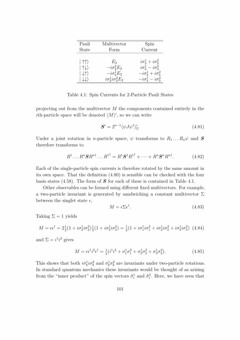
Pauli Multivector SpinState Form Current

| ↑↑〉 E2 iσ13 + iσ2

3| ↑↓〉 −iσ2

2E2 iσ13 − iσ2

3| ↓↑〉 −iσ1

2E2 −iσ13 + iσ2

3| ↓↓〉 iσ1

2iσ22E2 −iσ1

3 − iσ23

Table 4.1: Spin Currents for 2-Particle Pauli States

projecting out from the multivector M the components contained entirely in theith-particle space will be denoted 〈M〉i, so we can write

Si = 2n−1〈ψJψ†〉i2. (4.81)

Under a joint rotation in n-particle space, ψ transforms to R1 . . . Rnψ and S

therefore transforms to

R1 . . . RnSRn† . . . R1† = R1S1R1† + · · ·+RnSnRn†. (4.82)

Each of the single-particle spin currents is therefore rotated by the same amount inits own space. That the definition (4.80) is sensible can be checked with the fourbasis states (4.58). The form of S for each of these is contained in Table 4.1.

Other observables can be formed using different fixed multivectors. For example,a two-particle invariant is generated by sandwiching a constant multivector Σbetween the singlet state ε,

M = εΣε†. (4.83)

Taking Σ = 1 yields

M = εε† = 212(1 + iσ1

2iσ22)1

2(1 + iσ13iσ

23) = 1

2(1 + iσ11iσ

21 + iσ1

2iσ22 + iσ1

3iσ23) (4.84)

and Σ = i1i2 gives

M = εi1i2ε† = 12(i1i2 + σ1

1σ21 + σ1

2σ22 + σ1

3σ23). (4.85)

This shows that both iσ1kiσ

2k and σ1

kσ2k are invariants under two-particle rotations.

In standard quantum mechanics these invariants would be thought of as arisingfrom the “inner product” of the spin vectors σ1

i and σ2i . Here, we have seen that

101

the invariants arise in a completely different way by looking at the full multivectorεε†. It is interesting to note that the quantities iσ1

kiσ2k and σ1

kσ2k are similar in form

to the symplectic (doubling) bivector J introduced in Section 3.2.The contents of this section should have demonstrated that the multiparticle

STA approach is capable of reproducing most (if not all) of standard multiparticlequantum mechanics. One important result that follows is that the unit scalarimaginary j can be completely eliminated from quantum mechanics and replacedby geometrically meaningful quantities. This should have significant implicationsfor the interpretation of quantum mechanics. The main motivation for this workcomes, however, from the extension to relativistic quantum mechanics. There wewill part company with operator techniques altogether, and the multiparticle STAwill suggest an entirely new approach to relativistic quantum theory.

4.3 Dirac SpinorsWe now extend the procedures developed for Pauli spinors to show how Diracspinors can be understood in terms of the geometry of real spacetime. This revealsa geometrical role for spinors in the Dirac theory (a role which was first identified byHestenes [19, 21]). Furthermore, this formulation is representation-free, highlightingthe intrinsic content of the Dirac theory.

We begin with the γ-matrices in the standard Dirac-Pauli representation [59],

γ0 =(I 00 −I

)and γk =

(0 −σkσk 0

). (4.86)

A Dirac column spinor |ψ〉 is placed in one-to-one correspondence with an 8-component even element of the STA via [4, 61]

|ψ〉 =

a0 + ja3

−a2 + ja1

−b3 + jb0

−b1 − jb2

↔ ψ = a0 + akiσk + i(b0 + bkiσk). (4.87)

With the spinor |ψ〉 now replaced by an even multivector, the action of the operators

102

γµ, γ5, j (where γ5 = γ5 = −jγ0γ1γ2γ3) becomes

γµ |ψ〉 ↔ γµψγ0 (µ = 0, . . . , 3)j |ψ〉 ↔ ψ iσ3

γ5 |ψ〉 ↔ ψσ3,

(4.88)

which are verified by simple computation; for example

γ5 |ψ〉 =

−b3 + jb0

−b1 − jb2

a0 + ja3

−a2 + ja1

↔ −b3 + b0σ3 + b1iσ2 − b2iσ1

+a0σ3 + a3i− a2σ1 + a1σ2= ψσ3. (4.89)

Complex conjugation in this representation becomes

|ψ〉∗ ↔ −γ2ψγ2, (4.90)

which picks out a preferred direction on the left-hand side of ψ and so is not aLorentz-invariant operation.

As a simple application of (4.87) and (4.88), the Dirac equation

γµ(j∂µ − eAµ) |ψ〉 = m |ψ〉 (4.91)

becomes, upon postmultiplying by γ0,

∇ψiσ3 − eAψ = mψγ0 (4.92)

which is the form first discovered by Hestenes [17]. Here ∇ = γµ∂µ is the vectorderivative in spacetime. The properties of ∇ will be discussed more fully inChapter 6. This translation is direct and unambiguous, leading to an equationwhich is not only coordinate-free (since the vectors ∇ = γµ∂µ and A = γµAµno longer refer to any frame) but is also representation-free. In manipulating(4.92) one needs only the algebraic rules for multiplying spacetime multivectors,and the equation can be solved completely without ever having to introduce amatrix representation. Stripped of the dependence on a matrix representation,equation (4.92) expresses the intrinsic geometric content of the Dirac equation.

To discuss the spinor inner product, it is necessary to distinguish between the

103

Hermitian and Dirac adjoint. These are written as

〈ψ| − Dirac adjoint〈ψ| − Hermitian adjoint, (4.93)

which translate as follows,

〈ψ| ↔ ψ

〈ψ| ↔ ψ† = γ0ψγ0.(4.94)

This makes it clear that the Dirac adjoint is the natural frame-invariant choice.The inner product is handled in the same manner as in equation (4.21), so that

〈ψ |φ〉 ↔ 〈ψφ〉 − 〈ψφiσ3〉iσ3 = 〈ψφ〉S, (4.95)

which is also easily verified by direct calculation. In Chapters 6 and 7 we will beinterested in the STA form of the Lagrangian for the Dirac equation so, as anillustration of (4.95), this is given here:

L = 〈ψ|(γµ(j∂µ − eAµ)−m)|ψ〉 ↔ 〈∇ψiγ3ψ − eAψγ0ψ −mψψ〉. (4.96)

By utilising (4.95) the STA forms of the Dirac spinor bilinear covariants [60]are readily found. For example,

〈ψ|γµ |ψ〉 ↔ 〈ψγµψγ0〉 − 〈ψγµψiγ3〉iσ3 = γµ ·〈ψγ0ψ〉1 (4.97)

identifies the vector ψγ0ψ as the coordinate-free representation of the Dirac current.Since ψψ is even and reverses to give itself, it contains only scalar and pseudoscalarterms. We can therefore define

ρeiβ ≡ ψψ. (4.98)

Assuming ρ 6= 0, ψ can now be written as

ψ = ρ1/2eiβ/2R (4.99)

whereR = (ρeiβ)−1/2ψ. (4.100)

The even multivector R satisfies RR = 1 and is therefore a spacetime rotor. Double-

104

sided application of R on a vector a produces a Lorentz transformation. The STAequivalents of the full set of bilinear covariants [33] can now be written as

Scalar 〈ψ |ψ〉 ↔ 〈ψψ〉 = ρ cos βVector 〈ψ|γµ |ψ〉 ↔ ψγ0ψ = ρv

Bivector 〈ψ|jγµν |ψ〉 ↔ ψiσ3ψ = ρeiβS

Pseudovector 〈ψ|γµγ5 |ψ〉 ↔ ψγ3ψ = ρs

Pseudoscalar 〈ψ|jγ5 |ψ〉 ↔ 〈ψψi〉 = −ρ sin β,

(4.101)

wherev = Rγ0R

s = Rγ3R(4.102)

andS = isv. (4.103)

These are summarised neatly by the equation

ψ(1 + γ0)(1 + iγ3)ψ = ρ cosβ + ρv + ρeiβS + iρs+ iρ sinβ. (4.104)

The full Dirac spinor ψ contains (in the rotor R) an instruction to carry out arotation of the fixed γµ frame into the frame of observables. The analogy withrigid-body dynamics discussed in Section 4.1 therefore extends immediately to therelativistic theory. The single-sided transformation law for the spinor ψ is also“understood” in the same way that it was for Pauli spinors.

Once the spinor bilinear covariants are written in STA form (4.101) they canbe manipulated far more easily than in conventional treatments. For examplethe Fierz identities, which relate the various observables (4.101), are simple toderive [33]. Furthermore, reconstituting ψ from the observables (up to a gaugetransformation) is now a routine exercise, carried out by writing

〈ψ〉S = 14 (ψ + γ0ψγ0 − iσ3(ψ + γ0ψγ0)iσ3)

= 14(ψ + γ0ψγ0 + σ3ψσ3 + γ3ψγ3), (4.105)

so thatψ〈ψ〉S = 1

4ρ(eiβ + vγ0 − eiβSiσ3 + sγ3). (4.106)

The right-hand side of (4.106) can be found directly from the observables, and the

105

left-hand side gives ψ to within a complex multiple. On defining

Z = 14ρ(eiβ + vγ0 − eiβSiσ3 + sγ3) (4.107)

we find that, up to an arbitrary phase factor,

ψ = (ρeiβ)1/2Z(ZZ)−1/2. (4.108)

An arbitrary Dirac operator M |ψ〉 is replaced in the STA by a multilinearfunctionM(ψ), which acts linearly on the entire even subalgebra of the STA. The 64real dimensions of this space of linear operators are reduced to 32 by the constraint(4.39)

M(ψiσ3) = M(ψ)iσ3. (4.109)

Proceeding as at (4.44), the formula for the Dirac adjoint is

MDA(ψ) = ˜M(ψ). (4.110)

Self-adjoint Dirac operators satisfy M(ψ) = M(ψ) and include the γµ. TheHermitian adjoint, MHA, is derived in the same way:

MHA(ψ) = M †(ψ†), (4.111)

in agreement with the non-relativistic equation (4.44).Two important operator classes of linear operators on ψ are projection and

symmetry operators. The particle/antiparticle projection operators are replaced by

12m(m∓ γµpµ)|ψ〉 ↔ 1

2m(mψ ∓ pψγ0), (4.112)

and the spin-projection operators become

12(1± γµsµγ5)|ψ〉 ↔ 1

2(ψ ± sψγ3). (4.113)

Provided that p·s = 0, the spin and particle projection operators commute.The three discrete symmetries C, P and T translate equally simply (following

106

the convention of Bjorken & Drell [59]):

P |ψ〉 ↔ γ0ψ(x)γ0

C |ψ〉 ↔ ψσ1

T |ψ〉 ↔ iγ0ψ(−x)γ1,

(4.114)

where x = γ0xγ0 is (minus) a reflection of x in the time-like γ0 axis.The STA representation of the Dirac matrix algebra will be used frequently

throughout the remainder of this thesis. In particular, it underlies much of thegauge-theory treatment of gravity discussed in Chapter 7.

4.3.1 Changes of Representation — Weyl SpinorsIn the matrix theory, a change of representation is performed with a 4× 4 complexmatrix S. This defines new matrices

γ′µ = SγµS−1, (4.115)

with a corresponding spinor transformation |ψ〉 7→ S |ψ〉. For the Dirac equa-tion, it is also required that the transformed Hamiltonian be Hermitian, whichrestricts (4.115) to a unitary transformation

γ′µ = SγµS†, SS† = 1. (4.116)

The STA approach to handling alternative matrix representations is to find asuitable analogue of the Dirac-Pauli map (4.87) which ensures that the effect ofthe matrix operators is still given by (4.88). The relevant map is easy to constructonce the S is known which relates the new representation to the Dirac-Paulirepresentation. One starts with a column spinor |ψ〉′ in the new representation,constructs the equivalent Dirac-Pauli spinor S†|ψ〉′, then maps this into its STAequivalent using (4.87). This technique ensures that the action of j and the γµ, γ5matrices is still given by (4.88), and the C, P and T operators are still representedby (4.114). The STA form of the Dirac equation is always given by (4.92) and so isa truly representation-free expression.

The STA from of the Dirac and Hermitian adjoints is always given by theformulae (4.110) and (4.111) respectively. But the separate transpose and complexconjugation operations retain some dependence on representation. For example,

107

complex conjugation in the Dirac-Pauli representation is given by (4.90)

|ψ〉∗ ↔ −γ2ψγ2. (4.117)

In the Majorana representation, however, we find that the action of complex conju-gation on the Majorana spinor produces a different effect on its STA counterpart,

|ψ〉∗Maj ↔ ψσ2. (4.118)

In the operator/matrix theory complex conjugation is a representation-dependentconcept. This limits its usefulness for our representation-free approach. Instead, wethink of ψ 7→ −γ2ψγ2 and ψ 7→ ψσ2 as distinct operations that can be performedon the multivector ψ. (Incidentally, equation 4.118 shows that complex conjugationin the Majorana representation does indeed coincide with our STA form of thecharge conjugation operator (4.114), up to a conventional phase factor.)

To illustrate these techniques consider the Weyl representation, which is definedby the matrices [60]

γ′0 =(

0 −I−I 0

)and γ′k =

(0 −σkσk 0

). (4.119)

The Weyl representation is obtained from the Dirac-Pauli representation by theunitary matrix

u = 1√2

(I I

−I I

). (4.120)

A spinor in the Weyl representation is written as

|ψ〉′ =(|χ〉|η〉

), (4.121)

where |χ〉 and |η〉 are 2-component spinors. Acting on |ψ〉′ with u† gives

u†|ψ〉′ = 1√2

(|χ〉 − |η〉|χ〉+ |η〉.

)(4.122)

Using equation (4.87), this is mapped onto the even element

u†|ψ〉′ = 1√2

(|χ〉 − |η〉|χ〉+ |η〉

)↔ ψ = χ 1√

2(1 + σ3)− η 1√2(1− σ3), (4.123)

108

where χ and η are the Pauli-even equivalents of the 2-component complex spinors|χ〉 and |η〉, as defined by equation (4.9). The even multivector

ψ = χ 1√2(1 + σ3)− η 1√

2(1− σ3) (4.124)

is therefore our STA version of the column spinor

|ψ〉′ =(|χ〉|η〉

), (4.125)

where |ψ〉′ is acted on by matrices in the Weyl representation. As a check, weobserve that

γ′0|ψ〉′ =(−|η〉−|χ〉

)↔ −η 1√

2(1 + σ3) + χ 1√2(1− σ3) = γ0ψγ0 (4.126)

and

γk |ψ〉 =(−σk|η〉σk|χ〉

)↔ −σkησ3

1√2(1 + σ3)− σkχσ3

1√2(1− σ3) = γkψγ0.

(4.127)(We have used equation (4.12) and the fact that γ0 commutes with all Pauli-evenelements.) The map (4.123) does indeed have the required properties.

4.4 The Multiparticle Spacetime AlgebraWe now turn to the construction of the relativistic multiparticle STA. The principleis simple. We introduce a set of four (anticommuting) basis vectors γiµ, µ = 0 . . . 3,i = 1 . . . n where n is the number of particles. These vectors satisfy

γiµ ·γjν = δijηµν (4.128)

and so span a 4n-dimensional space. We interpret this as n-particle configurationspace. The construction of such a space is a standard concept in classical mechanicsand non-relativistic quantum theory, but the construction is rarely extended torelativistic systems. This is due largely to the complications introduced by aconstruction involving multiple times. In particular, Hamiltonian techniques appearto break down completely if a strict single-time ordering of events is lost. Butwe shall see that the multiparticle STA is ideally suited to the construction of

109

relativistic states. Furthermore, the two-particle current no longer has a positive-definite timelike component, so can describe antiparticles without the formalrequirement for field quantisation.

We will deal mainly with the two-particle STA. A two-particle quantum stateis represented in this algebra by the multivector ψ = ΨE, where E = E2 is thetwo-particle correlator (4.54) and Ψ is an element of the 64-dimensional directproduct space of the two even sub-algebras of the one-dimensional algebras. Thisconstruction ensures that ψ is 32-dimensional, as is required for a real equivalentof a 16-component complex column vector. Even elements from separate algebrasautomatically commute (recall (4.50)) so a direct product state has ψ = ψ1ψ2E =ψ2ψ1E. The STA equivalent of the action of the two-particle Dirac matrices γiµ isdefined by the operators

βiµ(ψ) = γiµψγi0. (4.129)

These operators satisfy

β1µβ

2µ(ψ) = γ1

µγ2µψγ

20γ

10 = γ2

µγ1µψγ

10γ

20 = β2

µβ1µ(ψ) (4.130)

and so, despite introducing a set of anticommuting vectors, the βiµ from differentparticle spaces commute. In terms of the matrix theory, we have the equivalences

γµ ⊗ I|ψ〉 ↔ β1µ(ψ), (4.131)

I ⊗ γµ|ψ〉 ↔ β2µ(ψ). (4.132)

Conventional treatments (e.g. Corson [62]) usually define the operators

βµ(ψ) = 12 [β1

µ(ψ) + β2µ(ψ)], (4.133)

which generate the well-known Duffin-Kemmer ring

βµβνβρ + βρβνβµ = ηνρβµ + ηνµβρ. (4.134)

This relation is verified by first writing

βνβρ(ψ) = 14 [(γνγρ)1ψ + (γνγρ)2ψ + γ1

νγ2ρψγ

20γ

10 + γ2

νγ1ρψγ

10γ

20 ](4.135)

⇒ βµβνβρ(ψ) = 18 [γ1

µνρψγ10 + γ2

µνρψγ20 + γ1

νργ2µψγ

20 + γ2

νργ1µψγ

10 +

γ1µνγ

2ρψγ

20 + γ2

µνγ1ρψγ

10 + γ1

µργ2νψγ

20 + γ2

µργ1νψγ

10 ] (4.136)

where γµν = γµγν etc. In forming βµβνβρ + βρβνβµ we are adding a quantity to its

110

reverse, which simply picks up the vector part of the products of vectors sitting onthe left-hand side of ψ in (4.136). We therefore find that

(βµβµβρ + βρβνβµ)ψ = 14 [〈γ1

µνρ + γ2νργ

1µ + γ2

µνγ1ρ + γ2

µργ1ν〉1ψγ1

0 +〈γ2µνρ + γ1

νργ2µ + γ1

µνγ2ρ + γ1

µργ2ν〉1ψγ2

0 ]= 1

2 [ηµνγ1ρ + ηνργ

1µ]ψγ1

0 + 12 [ηµνγ2

ρ + ηνργ2µ]ψγ2

0

= ηµνβρ(ψ) + ηνρβµ(ψ). (4.137)

The realisation of the Duffin-Kemmer algebra demonstrates that the multiparticleSTA contains the necessary ingredients to formulate the relativistic two-particleequations that have been studied in the literature.

The simplest relativistic two-particle wave equation is the Duffin-Kemmerequation (see Chapter 6 of [62]), which takes the form

∂µβµ(ψ)J = mψ. (4.138)

Here, ψ is a function of a single set of spacetime coordinates xµ, and ∂µ =∂xµ . Equation (4.138) describes a non-interacting field of spin 0 ⊕ 1. Since thewavefunction is a function of one spacetime position only, (4.138) is not a genuinetwo-body equation. Indeed, equation (4.138) has a simple one-body reduction,which is achieved by replacing ψ by a 4× 4 complex matrix [62, 63].

The first two-particle equation to consider in which ψ is a genuine function ofposition in configuration space is the famous Bethe-Salpeter equation [64]

(j∇1 −m1)(j∇2 −m2)|ψ(x1, x2)〉 = jI|ψ(x1, x2)〉 (4.139)

where ∇1 = γ1µ∂xµ1 etc. and I is an integral operator describing the inter-particle

interaction (Bethe & Salpeter [64] considered a relativistic generalisation of theYukawa potential). The STA version of (4.139) is

∇1∇2ψγ20γ

10 + [m1∇2ψγ2

0 +m2∇1ψγ10 − I(ψ)]J = m1m2ψ, (4.140)

where ∇1 and ∇2 are vector derivatives in the particle 1 and particle 2 spacesrespectively.

An alternative approach to relativistic two-body wave equations was initiated byBreit [65] in 1929. Breit wrote down an approximate two-body equation based onan equal-time approximation and applied this approximation to the fine structureof orthohelium. Breit’s approach was developed by Kemmer [66] and Fermi &

111

Yang [67], who introduced more complicated interactions to give phenomenologicaldescriptions of the deuteron and pions respectively. More recently, this workhas been extended by a number of authors (see Koide [68] and Galeõa & LealFerriara [63] and references therein). These approaches all make use of an equationof the type (in STA form)

Eψ + (γ10∧∇1 + γ2

0∧∇2)ψJ −m1γ0ψγ10 −m2γ2

0ψγ20 − I(ψ) = 0, (4.141)

where ψ = ψ(x1, x2) is a function of position in configuration space and I(ψ) againdescribes the inter-particle interaction. Equation (4.141) can be seen to arise froman equal-time approximation to the STA equation

γ10(∇1ψJ +m1ψγ1

0) + γ20(∇2ψJ +m1ψγ2

0)− I(ψ) = 0. (4.142)

In the case where the interaction is turned off and ψ is a direct-product state,

ψ = ψ1(x1)ψ2(x2)E, (4.143)

equation (4.142) recovers the single-particle Dirac equations for the two separateparticles. (This is also the case for the Bethe-Salpeter equation (4.139).) Thepresence of the γ1

0 and γ20 on the left-hand side mean that equation (4.142) is not

Lorentz covariant, however, so can at best only be an approximate equation. Fromthe STA form (4.139), one can immediately see how to proceed to a fully covariantequation. One simply removes the γ0’s from the left. The resultant equation is

(∇1ψγ10 +∇2ψγ2

0)J − I(ψ) = (m1 +m2)ψ, (4.144)

and indeed such an equation has recently been proposed by Krolikowski [69, 70](who did not use the STA).

These considerations should make it clear that the multiparticle STA is entirelysufficient for the study of relativistic multiparticle wave equations. Furthermore,it removes the need for either matrices or an (uninterpreted) scalar imaginary.But, in writing down (4.144), we have lost the ability to recover the single-particleequations. If we set I(ψ) to zero and use (4.143) for ψ, we find that(

ψ2(∇ψiγ3)1 + ψ1(∇ψiγ3)2 − (m1 +m2)ψ1ψ2)E = 0. (4.145)

112

On dividing through by ψ1ψ2 we arrive at the equation

(ψ1)−1(∇ψiγ3)1 + (ψ2)−1(∇ψiγ3)2 −m1 −m2 = 0, (4.146)

and there is now no way to ensure that the correct mass is assigned to the appropriateparticle.

There is a further problem with the equations discussed above. A multiparticleaction integral will involve integration over the entire 4n-dimensional configurationspace. In order that boundary terms can be dealt with properly (see Chapter 6)such an integral should make use of the configuration space vector derivative∇ = ∇1 +∇2. This is not the case for the above equations, in which the ∇1 and∇2 operators act separately. We require a relativistic two-particle wave equationfor particles of different masses which is derivable from an action integral andrecovers the individual one-particle equations in the absence of interactions. Insearching for such an equation we are led to an interesting proposal — one thatnecessitates parting company with conventional approaches to relativistic quantumtheory. To construct a space on which the full ∇ can act, the 32-dimensionalspinor space considered so far is insufficient. We will therefore extend our spinorspace to the the entire 128-dimensional even subalgebra of the two-particle STA.Right multiplication by the correlator E then reduces this to a 64-dimensionalspace, which is now sufficient for our purposes. With ψ now a member of this64-dimensional space, a suitable wave equation is

(∇1

m1 + ∇2

m2 )ψJ − ψ(γ10 + γ2

0)− I(ψ) = 0. (4.147)

The operator (∇1/m1 +∇2/m2) is formed from a dilation of ∇, so can be easily in-corporated into an action integral (this is demonstrated in Chapter 6). Furthermore,equation (4.147) is manifestly Lorentz covariant. In the absence of interactions,and with ψ taking the form of (4.143), equation (4.147) successfully recovers thetwo single-particle Dirac equations. This is seen by dividing through by ψ1ψ2 toarrive at (

1ψ1∇1

m1ψ1iσ1

3 + 1ψ2∇2

m2ψ2iσ2

3 − γ10 − γ2

0

)E = 0. (4.148)

The bracketed term contains the sum of elements from the two separate spaces, so

113

both terms must vanish identically. This ensures that

1ψ1∇1

m1ψ1iσ1

3 = γ10

⇒ ∇1ψ1iσ13 = m1ψ1γ1

0 , (4.149)

with the same result holding in the space of particle two. The fact that the particlemasses are naturally attached to their respective vector derivatives is interesting,and will be mentioned again in the context of the STA gauge theory of gravity(Chapter 7).

No attempt at solving the full equation (4.147) for interacting particles willbe made here (that would probably require a thesis on its own). But it is worthdrawing attention to a further property of the equation. The current conjugate togauge transformations is given by

j = j1

m1 + j2

m2 (4.150)

where j1 and j2 are the projections of 〈ψ(γ10 + γ2

0)ψ〉1 into the individual particlespaces. The current j satisfies the conservation equation

∇·j = 0 (4.151)

or(∇

1

m1 + ∇2

m2 )·〈ψ(γ10 + γ2

0)ψ〉1 = 0. (4.152)

For the direct-product state (4.143) the projections of j into the single-particlespaces take the form

j1 = 〈ψ2ψ2〉(ψ1γ10 ψ

1)j2 = 〈ψ1ψ1〉(ψ2γ2

0 ψ2). (4.153)

But the quantity 〈ψψ〉 is not positive definite, so the individual particle currentsare no longer necessarily future-pointing. These currents can therefore describeantiparticles. (It is somewhat ironic that most of the problems associated withthe single-particle Dirac equation can be traced back to the fact that the timelikecomponent of the current is positive definite. After all, producing a positive-definite density was part of Dirac’s initial triumph.) Furthermore, the conservationlaw (4.151) only relates to the total current in configuration space, so the projectionsonto individual particle spaces have the potential for very strange behaviour. For

114

example, the particle 1 current can turn round in spacetime, which would beinterpreted as an annihilation event. The interparticle correlations induced bythe configuration-space current j also afford insights into the non-local aspects ofquantum theory. Equation (4.147) should provide a fruitful source of future research,as well as being a useful testing ground for our ideas of quantum behaviour.

4.4.1 The Lorentz Singlet StateReturning to the 32-dimensional spinor space of standard two-particle quantumtheory, our next task is to find a relativistic analogue of the Pauli singlet statediscussed in Section 4.2.1. Recalling the definition of ε (4.70), the property thatensured that ε was a singlet state was that

iσ1kε = −iσ2

kε, k = 1 . . . 3. (4.154)

In addition to (4.154), a relativistic singlet state, which we will denote as η, mustsatisfy

σ1kη = −σ2

kη, k = 1 . . . 3. (4.155)

It follows that η satisfies

i1η = σ11σ

12σ

13η = −σ2

3σ22σ

21η = i2η (4.156)

so that

η = −i1i2η (4.157)⇒ η = 1

2(1− i1i2)η. (4.158)

Such a state can be formed by multiplying ε by the idempotent (1− i1i2)/2. Wetherefore define

η ≡ ε12(1− i1i2) = 1√

2(iσ12 − iσ2

2)12(1− iσ1

3iσ23)1

2(1− i1i2). (4.159)

This satisfiesiσ1kη = iσ1

kε12(1− i1i2) = −iσ2

kη k = 1 . . . 3 (4.160)

andσ1kη = −σ1

ki1i2η = i2iσ2

kη = −σ2kη k = 1 . . . 3. (4.161)

115

These results are summarised by

M1η = M2η, (4.162)

where M is an even multivector in either the particle 1 or particle 2 STA. Theproof that η is a relativistic invariant now reduces to the simple identity

R1R2η = R1R1η = η, (4.163)

where R is a relativistic rotor acting in either particle-one or particle-two space.Equation (4.162) can be seen as arising from a more primitive relation between

vectors in the separate spaces. Using the result that γ10γ

20 commutes with η, we

can derive

γ1µηγ

10 = γ1

µγ10γ

20ηγ

20γ

10γ

10

= γ20(γµγ0)1ηγ2

0

= γ20γ

20γ

2µηγ

20

= γ2µηγ

20 , (4.164)

and hence we find that, for an arbitrary vector a,

a1ηγ10 = a2ηγ2

0 . (4.165)

Equation (4.162) follows immediately from (4.165) by writing

(ab)1η = a1b1ηγ10γ

10

= a1b2ηγ20γ

10

= b2a1ηγ10γ

20

= b2a2ηγ20γ

20

= (ba)2η. (4.166)

Equation (4.165) can therefore be viewed as the fundamental property of therelativistic invariant η.

From η a number of Lorentz-invariant two-particle multivectors can be con-structed by sandwiching arbitrary multivectors between η and η. The simplest

116

such object is

ηη = ε12(1− i1i2)ε

= 12(1 + iσ1

1iσ21 + iσ1

2iσ22 + iσ1

3iσ23)1

2(1− i1i2)= 1

4(1− i1i2)− 14(σ1

kσ2k − iσ1

kiσ2k). (4.167)

This contains a scalar + pseudoscalar term, which is obviously invariant, togetherwith the invariant grade-4 multivector (σ1

kσ2k − iσ1

kiσ2k). The next simplest object is

ηγ10γ

20 η = 1

2(1 + iσ11iσ

21 + iσ1

2iσ22 + iσ1

3iσ23)1

2(1− i1i2)γ10γ

20

= 14(γ1

0γ20 + i1i2γ1

kγ2k − i1i2γ1

0γ20 − γ1

kγ2k)

= 14(γ1

0γ20 − γ1

kγ2k)(1− i1i2). (4.168)

On defining the symplectic (doubling) bivector

J ≡ γ1µγ

µ2 (4.169)

and the two-particle pseudoscalar

I ≡ i1i2 = i2i1 (4.170)

the invariants from (4.168) are simply J and IJ . As was disussed in Section (3.2),the bivector J is independent of the choice of spacetime frame, so is unchanged bythe two-sided application of the rotor R = R1R2. It follows immediately that the6-vector IJ is also invariant.

From the definition of J (4.169), we find that

J∧J = −2γ10γ

20γ

1kγ

2k + (γ1

kγ2k)∧(γ1

j γ2j )

= 2(σ1kσ

2k − iσ1

kiσ2k), (4.171)

which recovers the 4-vector invariant from (4.167). The complete set of two-particleinvariants can therefore be constructed from J alone, and these are summarisedin Table 4.2. These invariants are well-known and have been used in constructingphenomenological models of interacting particles [63, 68]. The STA derivation ofthe invariants is quite new, however, and the role of the doubling bivector J hasnot been previously noted.

117

Type ofInvariant Interaction Grade

1 Scalar 0J Vector 2

J∧J Bivector 4IJ Pseudovector 6I Pseudoscalar 8

Table 4.2: Two-Particle Relativistic Invariants

4.5 2-Spinor CalculusWe saw in Section 4.3.1 how spinors in the Weyl representation are handled withinthe (single-particle) STA. We now turn to a discussion of how the 2-spinor calculusdeveloped by Penrose & Rindler [36, 37] is formulated in the multiparticle STA.From equation (4.87), the chiral projection operators 1

2(1± γ′5) result in the STAmultivectors

12(1 + γ′5)|ψ〉′ ↔ ψ 1

2(1 + σ3) = χ 1√2(1 + σ3)

12(1− γ′5)|ψ〉′ ↔ ψ 1

2(1− σ3) = −η 1√2(1− σ3). (4.172)

The 2-spinors |χ〉 and |η〉 can therefore be given the STA equivalents

|χ〉 ↔ χ 1√2(1 + σ3)

|η〉 ↔ −η 1√2(1− σ3). (4.173)

These differ from the representation of Pauli spinors, and are closer to the “minimalleft ideal” definition of a spinor given by some authors (see Chapter 2 of [13], forexample). Algebraically, the (1 ± σ3) projectors ensure that the 4-dimensionalspaces spanned by elements of the type χ 1√

2(1 + σ3) and η 1√2(1− σ3) are closed

under left multiplication by a relativistic rotor. The significance of the (1 ± σ3)projectors lies not so much in their algebraic properties, however, but in the factthat they are the γ0-space projections of the null vectors γ0± γ3 . This will becomeapparent when we construct some 2-spinor “observables”.

Under a Lorentz transformation the spinor ψ transforms to Rψ, where R is a

118

relativistic rotor. If we separate the rotor R into Pauli-even and Pauli-odd terms,

R = R+ +R− (4.174)

where

R+ = 12(R + γ0Rγ0) (4.175)

R− = 12(R− γ0Rγ0), (4.176)

then we can write

Rχ 1√2(1 + σ3) = R+χ

1√2(1 + σ3) +R−χσ3

1√2(1 + σ3)

Rη 1√2(1− σ3) = R+η

1√2(1− σ3)−R−ησ3

1√2(1− σ3). (4.177)

The transformation laws for the Pauli-even elements χ and η are therefore

χ 7→ R+χ+R−χσ3 (4.178)η 7→ R+η −R−ησ3, (4.179)

which confirms that |χ〉 transforms under the operator equivalent of R, but that|η〉 transforms under the equivalent of

R+ −R− = γ0Rγ0 = (γ0Rγ0) = (R−1)†. (4.180)

This split of a Lorentz transformations into two distinct operations is an unattractivefeature of the 2-spinor formalism, but it is an unavoidable consequence of attemptingto perform relativistic calculations within the Pauli algebra of 2× 2 matrices. Theproblem is that the natural anti-involution operation is Hermitian conjugation.This operation is dependent on the choice of a relativistic timelike vector, whichbreaks up expressions in a way that disguises their frame-independent meaning.

The 2-spinor calculus attempts to circumvent the above problem by augmentingthe basic 2-component spinor with a number of auxilliary concepts. The result is alanguage which has proved to be well-suited to the study of spinors in a wide class ofproblems and it is instructive to see how some features of the 2-spinor are absorbedinto the STA formalism. The central idea behind the 2-spinor calculus is that atwo-component complex spinor |κ〉, derived form the Weyl representation (4.121),is replaced by the complex “vector” κA. Here the A is an abstract index labelingthe fact that κA is a single spinor belonging to some complex, two-dimensional

119

linear space. We represent this object in the STA as

κA ↔ κ12(1 + σ3). (4.181)

(The factor of 1/2 replaces 1/√

2 simply for convenience in some of the manipulationsthat follow.) The only difference now is that, until a frame is chosen in spin-space,we have no direct mapping between the components of κA and κ. Secifying a framein spin space also picks out a frame in spacetime (determined by the null tetrad).If this spacetime frame is identified with the γµ frame, then the components κA

of κA specify the Pauli-even multivector κ via the identification of equation (4.9).A second frame in spin-space produces different components κA, and will require adifferent identification to equation (4.9), but will still lead to the same multivectorκ1

2(1 + σ3). 2-Spinors are equipped with a Lorentz-invariant inner product derivedfrom a metric tensor εAB. This is used to lower indices so, for every 2-spinorκA, there is a corresponding κA. Both of these must have the same multivectorequivalent, however, in the same way that aµ and aµ both have the STA equivalenta.

To account for the second type of relativistic 2-spinor, |η〉 (4.121), a secondlinear space (or module) is introduced and elements of this space are labeled withbars and primed indices. Thus an abstract element of this space is written as ωA′ .In a given basis, the components of ωA′ are related to those of ωA by complexconjugation,

ω0′ = ω0, ω1′ = ω1. (4.182)

To construct the STA equivalent of ωA′ we need a suitable equivalent for thisoperation. Our equivalent operation should satisfy the following criteria:

1. The operation can only affect the right-hand side ω(1+σ3)/2, so that Lorentzinvariance is not compromised;

2. From equation (4.173), the STA equivalent of ωA′ must be a multivectorprojected by the (1− σ3)/2 idempotent, so the conjugation operation mustswitch idempotents;

3. The operation must square to give the identity;

4. The operation must anticommute with right-multiplication by iσ3.

The only operation satisfying all of these criteria is right-multiplication by somecombination of σ1 and σ2. Choosing between these is again a matter of convention,

120

so we will represent 2-spinor complex conjugation by right-multiplication by −σ1.It follows that our representation for the abstract 2-spinor ωA′ is

ωA′ ↔ −ω 1

2(1 + σ3)σ1 = −ωiσ212(1− σ3). (4.183)

Again, once a basis is chosen, ω is constructed using the identification of equa-tion (4.9) with the components ω0 = ω0′ and ω1 = ω1′ .

4.5.1 2-Spinor ObservablesOur next step in the STA formulation of 2-spinor calculus is to understand how torepresent quantities constructed from pairs of 2-spinors. The solution is remarkablysimple. One introduces a copy of the STA for each spinor, and then simplymultiplies the STA elements together, incorporating suitable correlators as oneproceeds. For example, the quantity κAκA′ becomes

κAκA′ ↔ −κ1 1

2(1 + σ13)κ2iσ2

212(1− σ2

3)12(1− iσ1

3iσ23). (4.184)

To see how to manipulate the right-hand side of (4.184) we return to the relativistictwo-particle singlet η (4.159). The essential property of η under multiplicationby even elements was equation (4.162). This relation is unaffected by furthermultiplication of η on the right-hand side by an element that commutes with E.We can therefore form the object

ε = η 12(1 + σ1

3) (4.185)

(not to be confused with the non-relativistic Pauli singlet state) which will stillsatisfy

M1ε = M2ε (4.186)

for all even multivectors M . The 2-particle state ε is still a relativistic singlet inthe sense of equation (4.163). From (4.185) we see that ε contains

12(1− i1i2)1

2(1 + σ13)1

2(1− iσ13iσ

23) = 1

2(1− iσ13i

2)12(1 + σ1

3)E= 1

2(1− iσ23i

2)12(1 + σ1

3)E= 1

2(1 + σ23)1

2(1 + σ13)E, (4.187)

so we can writeε = 1√

2(iσ12 − iσ2

2)12(1 + σ2

3)12(1 + σ1

3)E. (4.188)

121

A second invariant is formed by right-sided multiplication by (1− σ13)/2, and we

defineε = η 1

2(1− σ13). (4.189)

Proceeding as above, we find that

ε = 1√2(iσ1

2 − iσ22)1

2(1− σ23)1

2(1− σ13)E. (4.190)

This split of the full relativistic invariant η into ε and ε lies at the heart of much ofthe 2-spinor calculus. To see why, we return to equation (4.184) and from this weextract the quantity 1

2(1 + σ13)1

2(1− σ23)1

2(1− iσ13iσ

23). This can be manipulated as

follows:

12(1 + σ1

3)12(1− σ2

3)E = γ10

12(1− σ1

3)12(1− σ1

3)12(1− σ2

3)Eγ10

= γ10iσ

22

12(1− σ1

3)(−iσ22)1

2(1− σ13)1

2(1− σ23)Eγ1

0

= γ10iσ

22

12(1− σ1

3)(iσ12 − iσ2

2)12(1− σ1

3)12(1− σ2

3)Eγ10

= γ10iσ

22

1√2(1− σ1

3)εγ10

= − 1√2(γ1

0 + γ13)iσ1

2 εγ10 , (4.191)

which shows how an ε arises naturally in the 2-spinor product. This ε is thenused to project everything to its left back down to a single-particle space. Wecontinue to refer to each space as a “particle space” partly to stress the analogywith relativistic quantum states, but also simply as a matter of convenience. In2-spinor calculus there is no actual notion of a particle associated with each copyof spacetime.

Returning to the example of κAκA′ (4.184), we can now write

−κ1 12(1 + σ1

3)κ2iσ22

12(1− σ2

3)E = −κ1κ2iσ22

12(1 + σ1

3)12(1− σ2

3)E= κ1κ2 1√

2(γ10 + γ1

3)εγ10

= [κ 1√2(γ0 + γ3)κ]1εγ1

0 . (4.192)

The key part of this expression is the null vector κ(γ0 +γ3)κ/√

2, which is formed inthe usual STA manner by a rotation/dilation of the fixed null vector (γ0 + γ3)/

√2

by the even multivector κ. The appearance of the null vector (γ0 + γ3)/√

2 can betraced back directly to the (1 + σ3)/2 idempotent, justifying the earlier commentthat these idempotents have a clear geometric origin.

There are three further manipulations of the type performed in equation (4.191)

122

12(1 + σ1

3)12(1− σ2

3)E = − 1√2(γ1

0 + γ13)iσ1

2 εγ10

12(1− σ1

3)12(1 + σ2

3)E = − 1√2(γ1

0 − γ13)iσ1

2εγ10

12(1 + σ1

3)12(1 + σ2

3)E = − 1√2(σ1

1 + iσ12)ε

12(1− σ1

3)12(1− σ2

3)E = − 1√2(−σ1

1 + iσ12)ε

Table 4.3: 2-Spinor Manipulations

and the results of these are summarised in Table 4.3. These results can be used tofind a single-particle equivalent of any expression involving a pair of 2-spinors. Wewill see shortly how these reductions are used to construct a null tetrad, but firstwe need to find an STA formulation of the 2-spinor inner product.

4.5.2 The 2-spinor Inner Product.

Spin-space is equipped with an anti-symmetric inner product, written as eitherκAωA or κAωBεAB. In a chosen basis, the inner product is calculated as

κAωA = κAωA = κ0ω1 − κ1ω0, (4.193)

which yields a Lorentz-invariant complex scalar. The antisymmetry of the innerproduct suggests forming the STA expression

12(κAωB − ωAκB) ↔ 1

2(κ1ω2 − κ2ω1)12(1 + σ1

3)12(1 + σ2

3)E

= −12

(κ 1√

2(σ1 + iσ2)ω − 1√2ω(σ1 + iσ2)κ

)1ε

= − 1√2〈κ(σ1 + iσ2)ω〉10,4ε. (4.194)

The antisymmetric product therefore picks out the scalar and pseudoscalar partsof the quantity κ(σ1

1 + iσ12)ω. This is sensible, as these are the two parts that are

invariant under Lorentz transformations. Fixing up the factor suitably, our STArepresentation of the 2-spinor inner product will therefore be

κAωA ↔ −〈κ(σ1 + iσ2)ω〉0,4 = −〈κiσ2ω〉+ i〈κiσ1ω〉. (4.195)

That this agrees with the 2-spinor form in a given basis can be checked simply byexpanding out the right-hand side of (4.195).

A further insight into the role of the 2-spinor inner product is gained by

123

assembling the full even multivector (an STA spinor)

ψ = κ12(1 + σ3) + ωiσ2

12(1− σ3). (4.196)

The 2-spinor inner product can now be written as

ψψ = [κ12(1 + σ3) + ωiσ2

12(1− σ3)][−1

2(1 + σ3)iσ2ω + 12(1− σ3)κ]

= −κ12(1 + σ3)iσ2ω + ωiσ2

12(1− σ3)κ

= −〈κ(σ1 + iσ2)ω〉0,4 (4.197)

which recovers (4.195). The 2-spinor inner product is therefore seen to pick up boththe scalar and pseudoscalar parts of a full Dirac spinor product ψψ. Interchangingκ and ω in ψ (4.196) is achieved by right-multiplication by σ1, which immediatelyreverses the sign of ψψ. An important feature of the 2-spinor calculus has nowemerged, which is that the unit scalar imaginary is playing the role of the spacetimepseudoscalar. This is a point in favour of 2-spinors over Dirac spinors, but it isonly through consistent employment of the STA that this point has become clear.

The general role of the εAB tensor when forming contractions is also now clear.In the STA treatment, εAB serves to antisymmetrise on the two particle indicescarried by its STA equivalent. (It also introduces a factor of

√2, which is a result

of the conventions we have adopted.) This antisymmetrisation always resultsin a scalar + pseudoscalar quantity, and the pseudoscalar part can always bepulled down to an earlier copy of spacetime. In this manner, antisymmetrisationalways removes two copies of spacetime, as we should expect from the contractionoperation.

4.5.3 The Null TetradAn important concept in the 2-spinor calculus is that of a spin-frame. This consistsof a pair of 2-spinors, κA and ωA say, normalised such that κAωA = 1. In terms ofthe full spinor ψ (4.196), this normalisation condition becomes ψψ = 1. But this issimply the condition which ensures that ψ is a spacetime rotor! Thus the role of a“normalised spin-frame” in 2-spinor calculus is played by a spacetime rotor in theSTA approach. This is a considerable conceptual simplification. Furthermore, itdemonstrates how elements of abstract 2-spinor space can be represented in termsof geometrically meaningful objects — a rotor, for example, being simply a productof an even number of unit vectors.

124

Attached to the concept of a spin-frame is that of a null tetrad. Using κA andωA as the generators of the spin frame, the null tetrad is defined as follows:

la = κAκA′ ↔ −κ1κ2 1

2(1 + σ13)iσ2

212(1− σ2

3)E= 1√

2 [κ(γ0 + γ3)κ]1εγ10

= [ψ 1√2(γ0 + γ3)ψ]1εγ1

0 , (4.198)

na = ωAωA′ ↔ −ω1ω2 1

2(1 + σ13)iσ2

12(1− σ2

3)E= 1√

2 [ω(γ0 + γ3)ω]1εγ10

= [ψ 1√2(γ0 − γ3)ψ]1εγ1

0 , (4.199)

ma = κAωA′ ↔ −κ1ω2 1

2(1 + σ13)iσ2

12(1− σ2

3)E= 1√

2 [κ(γ0 + γ3)ω]1εγ10

= [ψ 1√2(γ1 + iγ2)ψ]1εγ1

0 , (4.200)

and

ma = ωAκA′ ↔ −ω1κ2 1

2(1 + σ13)iσ2

12(1− σ2

3)E= 1√

2 [ω(γ0 + γ3)κ]1εγ10

= [ψ 1√2(γ1 − iγ2)ψ]1εγ1

0 . (4.201)

The key identity used to arrive at the final two expression is

ψ(γ1 + iγ2)ψ = ψ(1 + σ3)γ1ψ

= κ(1 + σ3)γ1ψ

= −κγ1(1 + σ3)iσ2ω

= −κγ1(1 + σ3)σ1ω

= κ(γ0 + γ3)ω. (4.202)

The simplest spin frame is formed when ψ = 1. In this case we arrive at the

125

following comparison with page 120 of Penrose & Rindler [36];

la = 1√2(ta + za) ↔ 1√

2(γ0 + γ3)na = 1√

2(ta − za) ↔ 1√2(γ0 − γ3)

ma = 1√2(xa − jya) ↔ 1√

2(γ1 + iγ2)ma = 1√

2(xa + jya) ↔ 1√2(γ1 − iγ2).

(4.203)

The significant feature of this translation is that the “complex vectors” ma andma have been replaced by vector + trivector combinations. This agrees withthe observation that the imaginary scalar in the 2-spinor calculus plays the roleof the spacetime pseudoscalar. We can solve (4.203) for the Minkowski frameta, xa, ya, za (note how the abstract indices here simply record the fact that thet . . . z are vectors). The only subtlety is that, in recovering the vector ya from ourexpression for jya, we must post-multiply our 2-particle expression by iσ1

3. Thefactor of (1 + σ1

3) means that at the one-particle level this operation reduces toright-multiplication by i. We therefore find that

ta ↔ γ0 ya ↔ −γ2

xa ↔ γ1 za ↔ γ3.(4.204)

The only surprise here is the sign of the y-vector γ2. This sign can be traced back tothe fact that Penrose & Rindler adopt an usual convention for the σ2 Pauli matrix(page 16). This is also reflected in the fact that they identify the quaternionswith vectors (page 22), and we saw in Section 1.2.3 that the quaternion algebra isgenerated by the spatial bivectors iσ1,−iσ2, iσ3.

An arbitrary spin-frame, encoded in the rotor R, produces a new null tetradsimply by Lorentz rotating the vectors in (4.203), yielding

l = R 1√2(γ0 + γ3)R, m = R 1√

2(γ1 + iγ2)R,n = R 1√

2(γ0 − γ3)R, m = R 1√2(γ1 − iγ2)R. (4.205)

In this manner, the (abstract) null tetrad becomes a set of four arbitrary vec-tor/trivector combinations in (4.205), satisfying the anticommutation relations [4]

12l, n = 1, 1

2m, m = 1, all others = 0. (4.206)

126

4.5.4 The ∇A′A OperatorThe final 2-spinor object that we need a translation of is the differential operator∇A′A. The translation of ∇A′A will clearly involve the vector derivative ∇ = γµ∂xµ

and this must appear in such a way that it picks up the correct transformation lawunder a rotation in two-particle space. These observations lead us to the object

∇A′A ↔ ∇1εγ10 , (4.207)

so that, under a rotation,

∇1εγ10 7→ R1R2∇1εγ1

0 = R1∇R2εγ10

= (R∇R)1εγ10 , (4.208)

and the ∇ does indeed inherit the correct vector transformation law. In thischapter we are only concerned with the “flat-space” vector derivative ∇; a suitableformulation for “curved-space” derivatives will emerge in Chapter 7. A feature ofthe way that the multiparticle STA is employed here is that each spinor κ(1 +σ3)/2is a function of position in its own spacetime,

κj 12(1 + σj3) = κj(xj)1

2(1 + σj3). (4.209)

When such an object is projected into a different copy of spacetime, the positiondependence must be projected as well. In this manner, spinors can be “pulled back”into the same spacetime as the differential operator ∇.

We are now in a position to form the contraction ∇A′AκBεAB. We know thatthe role of the εAB is to antisymmetrise on the relevant particle spaces (in this casethe 2 and 3 spaces), together with introducing a factor of

√2. Borrowing from the

2-spinor notation, we denote this operation as ε2,3. We can now write

∇A′AκA = ∇A′AκBεAB ↔ ∇1ε12γ10κ

3 12(1 + σ3

3)E3ε2,3, (4.210)

where we have introduced the notation εij for the ε invariant (singlet state) un-der joint rotations in the ith and jth copies of spacetime. Equation (4.210) is

127

manipulated to give

∇1ε12γ10κ

3 12(1 + σ3

3)E3ε2,3

= ∇1 1√2(iσ1

2 − iσ22)κ3 1

2(1 + σ13)1

2(1 + σ23)1

2(1 + σ33)E3ε2,3γ

10

= ∇1 1√2

(−iσ1

2〈(σ1 + iσ2)κ〉20,4 + 〈iσ2(σ1 + iσ2)κ〉20,4)

12(1 + σ1

3)ε23γ10E3(4.211)

and projecting down into particle-one space, the quantity that remains is

∇A′AκA ↔ ∇ 1√2 [iσ2〈κ(σ1 + iσ2)〉0,4 + 〈κ(σ1 + iσ2)iσ2〉0,4]1

2(1 + σ3)γ0. (4.212)

We now require the following rearrangement:

[iσ2〈κ(σ1 + iσ2)〉0,4 + 〈κ(σ1 + iσ2)iσ2〉0,4]12(1 + σ3)

= [iσ2(〈κiσ2〉 − i〈κiσ1〉)− 〈κ〉+ i〈κiσ3〉]12(1 + σ3)

= [−〈κ〉+ iσk〈κiσk〉]12(1 + σ3)

= −κ12(1 + σ3). (4.213)

Using this, we find that

∇A′AκA ↔ − 1√2∇κ

12(1 + σ3)γ0 = − 1√

2∇γ0κ12(1− σ3), (4.214)

where pulling the γ0 across to the left-hand side demonstrates how the ∇A′A

switches between idempotents (modules). Equation (4.214) essentially justifiesthe procedure described in this section, since the translation (4.214) is “obvious”from the Weyl representation of the Dirac algebra (4.119). The factor of 1/

√2

in (4.214) is no longer a product of our conventions, but is an unavoidable aspectof the 2-spinor calculus. It remains to find the equivalent to the above for theexpression ∇AA′ωA′ . The translation for ∇AA′ is obtained from that for ∇A′A byswitching the “particle” indices, so that

∇AA′ ↔ −∇2εγ20 = −∇1εγ1

0 . (4.215)

Then, proceeding as above, we find that

∇AA′ωA′ ↔ − 1√2∇ωiσ2

12(1 + σ3)γ0. (4.216)

128

4.5.5 ApplicationsThe above constitutes the necessary ingredients for a complete translation of the2-spinor calculus into the STA. We close this chapter by considering two importantapplications. It should be clear from both that, whilst the steps to achieve the STAform are often quite complicated, the end result is nearly always more compactand easier to understand than the original 2-spinor form. An objective of futureresearch in this subject is to extract from 2-spinor calculus the techniques whichare genuinely powerful and useful. These can then be imported into the STA,which will suitably enriched by so doing. The intuitive geometric nature of theSTA should then make these techniques available to a wider audience of physiciststhan currently employ the 2-spinor calculus.

The Dirac Equation

The Dirac equation in 2-spinor form is given by the pair of equations [36, page 222]

∇A′AκA = µωA′

∇AA′ωA′ = µκA.(4.217)

The quantity µ is defined to be m/√

2, where m is the electron mass. The factorof 1/

√2 demonstrates that such factors are intrinsic to the way that the ∇A′A

symbol encodes the vector derivative. The equations (4.217) translate to the pairof equations

∇κ12(1 + σ3)γ0 = mωiσ2

12(1− σ3)

−∇ωiσ212(1− σ3)γ0 = mκ1

2(1 + σ3). (4.218)

If we now define the full spinor ψ by

ψ = κ12(1 + σ3) + ωσ2

12(1− σ3) (4.219)

we find that

∇ψγ0 = m[ωσ212(1− σ3)−mκ1

2(1 + σ3)]i= −mψiσ3. (4.220)

We thus recover the STA version of the Dirac equation (4.92)

∇ψiσ3 = mψγ0. (4.221)

129

Of the pair of equations (4.217), Penrose & Rindler write “an advantage of the2-spinor description is that the γ-matrices disappear completely – and complicatedγ-matrix identities simply evaporate!” [36, page 221]. Whilst this is true, thecomment applies even more strongly to the STA form of the Dirac equation (4.221),in which complicated 2-spinor identities are also eliminated!

Maxwell’s Equations

In the 2-spinor calculus the real, antisymmetric tensor F ab is written as

F ab = ψABεA′B′ + εABψA

′B′ , (4.222)

where ψAB is symmetric on its two indices. We first need the STA equivalent ofψAB. Assuming initially that ψAB is arbitrary, we can write

ψAB ↔ ψ 12(1 + σ1

3)12(1 + σ2

3)E = ψ 12(1 + σ1

3)σ11ε, (4.223)

where ψ is an arbitrary element of the product space of the two single-particlePauli-even algebras. A complete basis for ψ is formed by all combinations of the 7elements 1, iσ1

k, iσ2k. The presence of the singlet ε allows all elements of second

space to be projected down into the first space, and it is not hard to see that thisaccounts for all possible even elements in the one-particle STA. We can thereforewrite

ψ 12(1 + σ1

3)σ11ε = M1ε, (4.224)

where M is an arbitrary even element. The condition that ψAB is symmetric onits two indices now becomes (recalling that ε is antisymmetric on its two particleindices)

M1ε = −M2ε = −M1ε (4.225)

⇒M = −M. (4.226)

This condition projects out from M the components that are bivectors in particle-one space, so we can write

ψAB ↔ F 1ε (4.227)

where F is now a bivector. For the case of electromagnetism, F is the Faradaybivector, introduced in Section (1.2.5). The complete translation of F ab is therefore

F ab ↔ F 1ε+ F 1εσ11σ

21 = F 1η (4.228)

130

where η is the full relativistic invariant.The 2-spinor form of the Maxwell equations an be written

∇A′BψACεBC = −JAA′ (4.229)

where JAA′ is a “real” vector (i.e. it has no trivector components). Recallingthe convention that εij denotes the singlet state in coupled i, j-space, the STAversion of equation (4.229) is

∇1ε12γ10F

3ε34ε2,4 = −J1ε13γ10 . (4.230)

This is simplified by the identity

ε12ε34ε2,4 = ε13, (4.231)

which is proved by expanding the left-hand side and then performing the antisym-metrisation. The resultant equation is

∇1F 3ε13 = −J1ε13, (4.232)

which has a one-particle reduction to

∇F = J. (4.233)

This recovers the STA form of the Maxwell equations [17]. The STA form isremarkably compact, makes use solely of spacetime quantities and has a numberof computational advantages over second-order wave equations [8]. The 2-spinorcalculus also achieves a first-order formulation of Maxwell’s equations, but at theexpense of some considerable abstractions. We will return to equation (4.233) inChapters 6 and 7.

131

Chapter 5

Point-particle Lagrangians

In this chapter we develop a multivector calculus as the natural extension of thecalculus of functions of a single parameter. The essential new tool required for sucha calculus is the multivector derivative, and this is described first. It is shown howthe multivector derivative provides a coordinate-free language for manipulatinglinear functions (forming contractions etc.). This supersedes the approach used inearlier chapters, where such manipulations were performed by introducing a frame.

The remainder of this chapter then applies the techniques of multivector calculusto the analysis of point-particle Lagrangians. These provide a useful introductionto the techniques that will be employed in the study of field Lagrangians inthe final two chapters. A novel idea discussed here is that of a multivector-valued Lagrangian. Such objects are motivated by the pseudoclassical mechanicsof Berezin & Marinov [39], but can only be fully developed within geometricalgebra. Forms of Noether’s theorem are given for both scalar and multivector-valued Lagrangians, and for transformations parameterised by both scalars andmultivectors. This work is applied to the study of two semi-classical models ofelectron spin. Some aspects of the work presented in this chapter appeared in thepapers “Grassmann mechanics, multivector derivatives and geometric algebra” [3]and “Grassmann calculus, pseudoclassical mechanics and geometric algebra” [1].

5.1 The Multivector DerivativeThe idea of a vector derivative was partially introduced in Chapter 4, where itwas seen that the STA form of the Dirac equation (4.92) required the operator∇ = γµ∂xµ , where xµ = γµ ·x. The same operator was later seen to appear in the

132

STA form of the Maxwell equations (4.233), ∇F = J . We now present a moreformal introduction to the properties of the vector and multivector derivatives.Further details of these properties are contained in [18] and [24, Chapter 2], thelatter of which is particularly detailed in its treatment.

Let X be a mixed-grade multivector

X =∑r

Xr, (5.1)

and let F (X) be a general multivector-valued function of X. The grades ofF (X) need not be the same as those of its argument X. For example, the STArepresentation of a Dirac spinor as ψ(x) is a map from the vector x onto an arbitraryeven element of the STA. The derivative of F (X) in the A direction, where A hasthe same grades as X, is defined by

A∗∂XF (X) ≡ limτ→0

F (X + τA)− F (X)τ

. (5.2)

(It is taken as implicit in this definition that the limit exists.) The operator A ∗ ∂Xsatisfies all the usual properties for partial derivatives. To define the multivectorderivative ∂X , we introduce an arbitrary frame ej and extend this to define abasis for the entire algebra eJ, where J is a general (simplicial) index. Themultivector derivative is now defined by

∂X =∑J

eJeJ ∗∂X . (5.3)

The directional derivative eJ ∗∂X is only non-zero when eJ is of the same grade(s)as X, so ∂X inherits the multivector properties of its argument X. The contractionin (5.3) ensures that the quantity ∂X is independent of the choice of frame, andthe basic properties of ∂X can be formulated without any reference to a frame.

The properties of ∂X are best understood with the aid of some simple examples.The most useful result for the multivector derivative is

∂X〈XA〉 = PX(A), (5.4)

where PX(A) is the projection of A on to the grades contained in X. From (5.4) itfollows that

∂X〈XA〉 = PX(A)∂X〈XA〉 = PX(A). (5.5)

133

Leibniz’ rule can now be used in conjunction with (5.4) to build up results for theaction of ∂X on more complicated functions. For example,

∂X〈XX〉k/2 = k〈XX〉(k−2)/2X. (5.6)

The multivector derivative acts on objects to its immediate right unless bracketsare present, in which case ∂X acts on the entire bracketed quantity. If ∂X acts on amultivector that is not to its immediate right, we denote this with an overdot onthe ∂X and its argument. Thus ∂XAB denotes the action of ∂X on B,

∂XAB = eJAeJ ∗∂XB. (5.7)

The overdot notation is an invaluable aid to expressing the properties of themultivector derivative. In particular, it neatly encodes the fact that, since ∂X isa multivector, it does not necessarily commute with other multivectors and oftenacts on functions to which it is not adjacent. As an illustration, Leibniz’ rule cannow be given in the form

∂X(AB) = ∂XAB + ∂XAB. (5.8)

The only drawback with the overdot notation comes in expressions which involvetime derivatives. It is usually convenient to represent these with overdots as well,and in such instances the overdots on multivector derivatives will be replaced byoverstars.

The most useful form of the multivector derivative is the derivative with respectto a vector argument, ∂a or ∂x. Of these, the derivative with respect to position xis particularly important. This is called the vector derivative, and is given specialthe symbol

∂x = ∇ = ∇x. (5.9)

The operator ∇ sometimes goes under the name of the Dirac operator, thoughthis name is somewhat misleading since ∂x is well-defined in all dimensions and isin no way tied to quantum-mechanical notions. In three dimensions, for example,∂x = ∇ contains all the usual properties of the div, grad and curl operators. Thereare a number of useful formulae for derivatives with respect to vectors, a selection

134

of which is as follows:

∂aa·b = b

∂aa2 = 2a

∂a ·a = n

∂a∧a = 0∂aa·Ar = rAr∂aa∧Ar = (n− r)Ar∂aAra = (−1)r(n− 2r)Ar,

(5.10)

where n is the dimension of the space. The final three equations in (5.10) are theframe-free forms of formulae given in Section (1.3.2).

Vector derivatives are very helpful for developing the theory of linear functions,as introduced in Section (1.3). For example, the adjoint to the linear function fcan be defined as

f(a) ≡ ∂b〈af(b)〉. (5.11)

It follows immediately that

b·f(a) = b·∂c〈af(c)〉 = 〈f(b·∂cc)a〉 = f(b)·a. (5.12)

Invariants can be constructed equally simply. For example, the trace of f(a) isdefined by

Trf ≡ ∂a ·f(a) (5.13)

and the “characteristic bivector” of f(a) is defined by

B = 12∂a∧f(a). (5.14)

An anti-symmetric function f = −f can always be written in the form

f(a) = a·B (5.15)

and it follows from equation (5.10) that B is the characteristic bivector.Many other aspects of linear algebra, including a coordinate-free proof of the

Cayley-Hamilton theorem, can be developed similarly using combinations of vectorderivatives [24, Chapter 3].

135

5.2 Scalar and Multivector LagrangiansAs an application of the multivector derivative formalism just outlined, we considerLagrangian mechanics. We start with a scalar-valued Lagrangian L = L(Xi, Xi),where the Xi are general multivectors, and Xi denotes differentiation with respectto time. We wish to find the Xi(t) which extremise the action

S =∫ t2

t1dt L(Xi, Xi). (5.16)

The solution to this problem can be found in many texts (see e.g. [71]). We write

Xi(t) = X0i (t) + εYi(t), (5.17)

where Yi is a multivector containing the same grades as Xi and which vanishesat the endpoints, ε is a scalar and X0

i represents the extremal path. The actionmust now satisfy ∂εS = 0 when ε = 0, since ε = 0 corresponds to Xi(t) taking theextremal values. By applying the chain rule and integrating by parts, we find that

∂εS =∫ t2

t1dt((∂εXi)∗∂XiL+ (∂εXi)∗∂XiL

)=

∫ t2

t1dt(Yi∗∂XiL+ Yi∗∂XiL

)=

∫ t2

t1dt Yi∗

(∂XiL− ∂t(∂XiL)

). (5.18)

Setting ε to zero now just says that Xi is the extremal path, so the extremal pathis defined by the solutions to the Euler-Lagrange equations

∂XiL− ∂t(∂XiL) = 0. (5.19)

The essential advantage of this derivation is that it employs genuine derivatives inplace of the less clear concept of an infinitessimal. This will be exemplified whenwe study Lagrangians containing spinor variables.

We now wish to extend the above argument to a multivector-valued LagrangianL. Taking the scalar product of L with an arbitrary constant multivector A producesa scalar Lagrangian 〈LA〉. This generates its own Euler-Lagrange equations,

∂Xi〈LA〉 − ∂t(∂Xi〈LA〉) = 0. (5.20)

136

A “permitted” multivector Lagrangian is one for which the equations from eachA are mutually consistent, so that each component of the full L is capable ofsimultaneous extremisation.

By contracting equation (5.20) on the right-hand side by ∂A, we find that anecessary condition on the dynamical variables is

∂XiL− ∂t(∂XiL) = 0. (5.21)

For a permitted multivector Lagrangian, equation (5.21) is also sufficient to ensurethat equation (5.20) is satisfied for all A. This is taken as part of the definition ofa multivector Lagrangian. We will see an example of how these criteria can be metin Section 5.3.

5.2.1 Noether’s TheoremAn important technique for deriving consequences of the equations of motionresulting from a given Lagrangian is the study of the symmetry properties of theLagrangian itself. The general result needed for this study is Noether’s theorem.We seek a form of this theorem which is applicable to both scalar-valued andmultivector-valued Lagrangians. There are two types of symmetry to consider,depending on whether the transformation of variables is governed by a scalar or bya multivector parameter. We will look at these separately.

It is important to recall at this point that all the results obtained here arederived in the coordinate-free language of geometric algebra. Hence all the symmetrytransformations considered are active. Passive transformations have no place in thisscheme, as the introduction of an arbitrary coordinate system is an unnecessarydistraction.

5.2.2 Scalar Parameterised TransformationsGiven a Lagrangian L = L(Xi, Xi), which can be either scalar-valued or multivector-valued, we wish to consider variations of the variables Xi controlled by a singlescalar parameter, α. We write this as

X ′i = X ′i(Xi, α), (5.22)

137

and assume that X ′i(α = 0) = Xi. We now define the new Lagrangian

L′(Xi, Xi) = L(X ′i, X ′i), (5.23)

which has been obtained from L by an active transformation of the dynamicalvariables. Employing the identity L′ = 〈L′A〉∂A, we proceed as follows:

∂αL′ = (∂αX ′i)∗∂X′i〈L

′A〉∂A + (∂aX ′i)∗∂X′i〈L′A〉∂A

= (∂aX ′i)∗(∂X′i〈L

′A〉 − ∂t(∂X′i〈L′A〉)

)∂A + ∂t

((∂aX ′i)∗∂X′iL

′).(5.24)

The definition of L′ ensures that it has the same functional form of L, so thequantity

∂X′i〈L′A〉 − ∂t(∂X′i〈L

′A〉)L′ (5.25)

is obtained by taking the Euler-Lagrange equations in the form (5.20) and replacingthe Xi by X ′i. If we now assume that the X ′i satisfy the same equations of motion(which must be checked for any given case), we find that

∂αL′ = ∂t

((∂aX ′i)∗∂X′iL

′)

(5.26)

and, if L′ is independent of α, the corresponding quantity (∂aX ′i)∗∂X′iL′ is conserved.

Alternatively, we can set α to zero so that (5.25) becomes

[∂X′i〈L′A〉 − ∂t(∂X′i〈L

′A〉)L′]∣∣∣α=0

= ∂Xi〈LA〉 − ∂t(∂Xi〈LA〉) (5.27)

which vanishes as a consequence of the equations of motion for Xi. We thereforefind that

∂aL′|α=0 = ∂t

((∂aX ′i)∗∂X′iL

′)∣∣∣α=0

, (5.28)

which is probably the most useful form of Noether’s theorem, in that interestingconsequences follow from (5.28) regardless of whether or not L′ is independent ofα. A crucial step in the derivation of (5.28) is that the Euler-Lagrange equationsfor a multivector-valued Lagrangian are satisfied in the form (5.20). Hence theconsistency of the equations (5.20) for different A is central to the development ofthe theory of multivector Lagrangians.

To illustrate equation (5.28), consider time translation

X ′i(t, α) = Xi(t+ α) (5.29)⇒ ∂aX

′i|α=0 = Xi. (5.30)

138

Assuming there is no explicit time-dependence in L, equation (5.28) gives

∂tL = ∂t(Xi∗∂XiL), (5.31)

from which we define the conserved Hamiltonian by

H = Xi∗∂XiL− L. (5.32)

If L is multivector-valued, then H will be a multivector of the same grade(s).

5.2.3 Multivector Parameterised TransformationsThe most general single transformation for the variables Xi governed by a multi-vector M can be written as

X ′i = f(Xi,M), (5.33)

where f and M are time-independent functions and multivectors respectively. Ingeneral f need not be grade-preserving, which provides a route to deriving analoguesfor supersymmetric transformations.

To follow the derivation of (5.26), it is useful to employ the differential notation[24],

fM

(Xi, A) ≡ A∗∂Mf(Xi,M). (5.34)

The function fM

(Xi, A) is a linear function of A and an arbitrary function of Mand Xi. With L′ defined as in equation (5.23), we derive

A∗∂ML′ = fM

(Xi, A)∗∂X′iL′ + f

M(Xi,M)∗∂X′iL

′

= fM

(Xi, A)∗(∂X′i〈L

′B〉 − ∂t(∂X′i〈L′B〉)

)∂B + ∂t

(fM

(Xi, A)∗∂X′iL′)

= ∂t(fM

(Xi, A)∗∂X′iL′), (5.35)

where again it is necessary to assume that the equations of motion are satisfiedfor the transformed variables. We can remove the A-dependence by differentiating,which yields

∂ML′ = ∂t

(∂AfM(Xi, A)∗∂X′iL

′)

(5.36)

and, if L′ is independent of M , the corresponding conserved quantity is

∂AfM(Xi, A)∗∂X′iL′ =∗∂M f(Xi,

∗M)∗∂X′iL

′, (5.37)

139

where the overstar on∗M denote the argument of

∗∂M .

It is not usually possible to set M to zero in (5.35), but it is interesting tosee that conserved quantities can be found regardless. This shows that standardtreatments of Lagrangian symmetries [71] are unnecessarily restrictive in onlyconsidering infinitesimal transformations. The subject is richer than this suggests,though without multivector calculus the necessary formulae are hard to find.

In order to illustrate (5.37), consider reflection symmetry applied to the harmonicoscillator Lagrangian

L(x, x) = 12(x2 − ω2x2). (5.38)

The equations of motion arex = −ω2x (5.39)

and it is immediately seen that, if x is a solution, then so to is x′, where

x′ = −nxn−1. (5.40)

Here n is an arbitrary vector, so x′ is obtained from x by a reflection in the hyper-plance orthogonal to n. Under the reflection (5.40) the Lagrangian is unchanged,so we can find a conserved quantity from equation (5.37). With f(x, n) defined by

f(x, n) = −nxn−1 (5.41)

we find thatfn(x, a) = −axn−1 + nxn−1an−1. (5.42)

Equation (5.37) now yields the conserved quantity

∂a(−axn−1 + nxn−1an−1)∗(−nxn−1) = ∂a〈axxn−1 − axxn−1〉= 〈xxn−1 − xxn−1〉1= 2(x∧x)·n−1. (5.43)

This is conserved for all n, from which it follows that the angular momentum x∧ xis conserved. This is not a surprise, since rotations can be built out of reflectionsand different reflections are related by rotations. It is therefore natural to expectthe same conserved quantity from both rotations and reflections. But the derivationdoes show that the multivector derivative technique works and, to my knowledge,this is the first time that a classical conserved quantity has been derived conjugateto transformations that are not simply connected to the identity.

140

5.3 Applications — Models for Spinning PointParticles

There have been numerous attempts to construct classical models for spin-halfparticles (see van Holten [72] for a recent review) and two such models are consideredin this section. The first involves a scalar point-particle Lagrangian in which thedynamical variables include spinor variables. The STA formalism of Chapter 4 isapplied to this Lagrangian and used to analyse the equations of motion. Someproblems with the model are discussed, and a more promising model is proposed.The second example is drawn from pseudoclassical mechanics. There the dynamicalvariables are Grassmann-valued entities, and the formalism of Chapter 2 is usedto represent these by geometric vectors. The resulting Lagrangian is multivector-valued, and is studied using the techniques just developed. The equations of motionare found and solved, and again it is argued that the model fails to provide anacceptable picture of a classical spin-half particle.

1. The Barut-Zanghi ModelThe Lagrangian of interest here was introduced by Barut & Zanghi [38] (seealso [7, 61]) and is given by

L = 12j(

˙ΨΨ− ΨΨ) + pµ(xµ − ΨγµΨ) + qAµ(x)ΨγµΨ (5.44)

where Ψ is a Dirac spinor. Using the mapping described in Section (4.3), theLagrangian (5.45) can be written as

L = 〈ψiσ3ψ + p(x− ψγ0ψ) + qA(x)ψγ0ψ〉. (5.45)

The dynamical variables are x, p and ψ, where ψ is an even multivector, and thedot denotes differentiation with respect to some arbitrary parameter τ .

The Euler-Lagrange equation for ψ is

∂ψL = ∂τ (∂ψL)

⇒ ∂τ (iσ3ψ) = −iσ3˙ψ − 2γ0ψp+ 2qγ0ψA

⇒ ψiσ3 = Pψγ0, (5.46)

141

whereP ≡ p− qA. (5.47)

In deriving (5.46) there is no pretence that ψ and ψ are independent variables.Instead they represent two occurrences of the same variable ψ and all aspects ofthe variational principle are taken care of by the multivector derivative.

The p equation isx = ψγ0ψ (5.48)

but, since x2 = ρ2 is not, in general, equal to 1, τ cannot necessarily be viewed asthe proper time for the particle. The x equation is

p = q∇A(x)·(ψγ0ψ)= q(∇∧A)·x+ qx·∇A

⇒ P = qF ·x. (5.49)

We now use (5.28) to derive some consequences for this model. The Hamiltonianis given by

H = x∗∂xL+ ψ∗∂ψL− L= P ·x, (5.50)

and is conserved absolutely. The 4-momentum and angular momentum are onlyconserved if A = 0, in which case (5.45) reduces to the free-particle Lagrangian

L0 = 〈ψiσ3ψ + p(x− ψγ0ψ)〉. (5.51)

The 4-momentum is found from translation invariance,

x′ = x+ αa, (5.52)

and is simply p. The component of p in the x direction gives the energy (5.50).The angular momentum is found from rotational invariance, for which we set

x′ = eαB/2xe−αB/2

p′ = eαB/2pe−αB/2

ψ′ = eαB/2ψ.

(5.53)

142

It is immediately apparent that L′0 is independent of α, so the quantity

(B ·x)∗∂xL0 + 12(Bψ)∗∂ψL0 = B ·(x∧p+ 1

2ψiσ3ψ) (5.54)

is conserved for arbitrary B. The angular momentum is therefore defined by

J = p∧x− 12ψiσ3ψ, (5.55)

which identifies −ψiσ3ψ/2 as the internal spin. The factor of 1/2 clearly originatesfrom the transformation law (5.53). The free-particle model defined by (5.51)therefore does have some of the expected properties of a classical model for spin,though there is a potential problem with the definition of J (5.55) in that the spincontribution enters with the opposite sign to that expected from field theory (seeChapter 6).

Returning to the interacting model (5.45), further useful properties can bederived from transformations in which the spinor is acted on from the right. Thesecorrespond to gauge transformations, though a wider class is now available thanfor the standard column-spinor formulation. From the transformation

ψ′ = ψeαiσ3 (5.56)

we find that∂τ 〈ψψ〉 = 0, (5.57)

and the transformationψ′ = ψeασ3 (5.58)

yields∂τ 〈iψψ〉 = −2P ·(ψγ3ψ). (5.59)

Equations (5.57) and (5.59) combine to give

∂τ (ψψ) = 2iP ·(ψγ3ψ). (5.60)

Finally, the duality transformation

ψ′ = ψeαi (5.61)

yields2〈ψσ3ψ〉 = 0. (5.62)

143

A number of features of the Lagrangian (5.45) make it an unsatisfactory modela classical electron. We have already mentioned that the parameter τ cannotbe identified with the proper time of the particle. This is due to the lack ofreparameterisation invariance in (5.45). More seriously, the model predicts a zerogyromagnetic moment [61]. Furthermore, the P equation (5.49) cannot be correct,since here one expects to see p rather than P coupling to F·x. Indeed, the definitionof P (5.47) shows that equation (5.49) is not gauge invariant, which suggests thatit is a lack of gauge invariance which lies behind some of the unacceptable featuresof the model.

2. Further Spin-half ModelsWe will now see how to modify the Lagrangian (5.45) to achieve a suitable setof classical equations for a particle with spin. The first step is to consider gaugeinvariance. Under the local gauge transformation

ψ 7→ ψ exp−iσ3φ(τ) (5.63)

the “kinetic” spinor term 〈ψiσ3ψ〉 transforms as

〈ψiσ3ψ〉 7→ 〈ψiσ3ψ〉+ 〈ψψφ〉. (5.64)

The final term can be written as

〈ψψφ〉 = 〈ψψx·(∇φ)〉, (5.65)

and, when ∇φ is generalised to an arbitrary gauge field qA, (5.64) produces theinteraction term

LI = q〈ψψx·A〉. (5.66)

This derivation shows clearly that the A field must couple to x and not to ψγ0ψ,as it is not until after the equations of motion are found that ψγ0ψ is set equal tox. That there should be an x·A term in the Lagrangian is natural since this is theinteraction term for a classical point particle, and a requirement on any action thatwe construct is that it should reproduce classical mechanics in the limit where spineffects are ignored (i.e. as h 7→ 0). But a problem still remains with (5.66) in thatthe factor of ψψ is unnatural and produces an unwanted term in the ψ equation..

144

To remove this, we must replace the 〈ψiσ3ψ〉 term by

L0 = 〈ψiσ3ψ−1〉, (5.67)

where, for a spinor ψ = (ρeiβ)1/2R,

ψ−1 = (ρeiβ)−1/2R. (5.68)

In being led the term (5.67), we are forced to break with conventional usageof column spinors. The term (5.67) now suggests what is needed for a suitableclassical model. The quantity 〈ψiσ3ψ

−1〉 is unchanged by both dilations and dualitytransformations of ψ and so is only dependent on the rotor part of ψ. It has beensuggested that the rotor part of ψ encodes the dynamics of the electron field andthat the factor of (ρ expiβ)1/2 is a quantum-mechanical statistical term [29].Accepting this, we should expect that our classical model should involve only therotor part of ψ and that the density terms should have no effect. Such a modelrequires that the Lagrangian be invariant under local changes of ρ expiβ, as wehave seen is the case for L0 (5.67). The remaining spinorial term is the currentterm ψγ0ψ which is already independent of the duality factor β. It can be madeindependent of the density ρ as well by dividing by ρ. From these observations weare led to the Lagrangian

L = 〈ψiσ3ψ−1 + p(x− ψγ0ψ/ρ)− qx·A〉. (5.69)

The p equation from (5.69) recovers

x = ψγ0ψ/ρ = Rγ0R, (5.70)

so that x2 = 1 and τ is automatically the affine parameter. This removes one ofthe defects with the Barut-Zanghi model. The x equation gives, using standardtechniques,

p = qF ·x, (5.71)

which is now manifestly gauge invariant and reduces to the Lorentz force law whenthe spin is ignored and the velocity and momentum are collinear, p = mx. Finally,the ψ equation is found by making use of the results

∂ψ〈ψMψ−1〉 = Mψ−1 + ∂ψ〈ψMψ−1〉 = 0 (5.72)

145

⇒ ∂ψ〈Mψ−1〉 = −ψ−1Mψ−1 (5.73)

and

∂ψρ = 12ρ∂ψ(ψγ0ψψγ0ψ)

= 2ργ0ρe

iβγ0ψ

= 2ρψ−1 (5.74)

to obtain

−ψ−1ψiσ3ψ−1 − 1

ρ(2γ0ψp− 2ψ−1〈pψγ0ψ〉) = ∂τ (iσ3ψ

−1). (5.75)

By multiplying equation (5.75) with ψ, one obtains

12 S = p∧x, (5.76)

whereS ≡ ψiσ3ψ

−1 = Riσ3R. (5.77)

Thus the ψ variation now leads directly to the precession equation for the spin.The complete set of equations is now

S = 2p∧x (5.78)x = Rγ0R (5.79)p = qF ·x (5.80)

which are manifestly Lorentz covariant and gauge invariant. The Hamiltonianis now p · x and the free-particle angular momentum is still defined by J (5.55),though now the spin bivector S is always of unit magnitude.

A final problem remains, however, which is that we have still not succeeded inconstructing a model which predicts the correct gyromagnetic moment. In orderto achieve the correct coupling between the spin and the Faraday bivector, theLagrangian (5.69) must be modified to

L = 〈ψiσ3ψ−1 + p(x− ψγ0ψ/ρ) + qx·A− q

2mFψiσ3ψ−1〉. (5.81)

146

The equations of motion are now

S = 2p∧x+ q

mF×S

x = Rγ0R (5.82)p = qF ·x− q

2m∇F (x)·S,

which recover the correct precession formulae in a constant magnetic field. Whenp is set equal to mx, the equations (5.82) reduce to the pair of equations studiedin [72].

3. A Multivector Model — Pseudoclassical Mechanics Re-consideredPseudoclassical mechanics [39, 73, 74] was originally introduced as the classicalanalogue of quantum spin one-half (i.e. for particles obeying Fermi statistics).The central idea is that the “classical analogue” of the Pauli or Dirac algebrasis an algebra where all inner products vanish, so that the dynamical variablesare Grassmann variables. From the point of view of this thesis, such an ideaappears fundamentally flawed. Furthermore, we have already seen how to constructsensible semi-classical approximations to Dirac theory. But once the Grassmannvariables have been replaced by vectors through the procedure outlined in Chapter 2,pseudoclassical Lagrangians do become interesting, in that they provide examplesof acceptable multivector Lagrangians. Such a Lagrangian is studied here, from anumber of different perspectives. An interesting aside to this work is a new methodof generating super-Lie algebras, which could form the basis for an alternativeapproach to their representation theory.

The Lagrangian we will study is derived from a pseudoclassical Lagrangianintroduced by Berezin & Marinov [39]. This has become a standard example innon-relativistic pseudoclassical mechanics [73, Chapter 11]. With a slight change ofnotation, and dropping an irrelevant factors of j, the Lagrangian can be written as

L = 12ζiζi −

12εijkωiζjζk, (5.83)

where the ζi are formally Grassmann variable and the ωi are a set of threescalar constants. Here, i runs from 1 to 3 and, as always, the summation conventionis implied. Replacing the set of Grassmann variables ζi with a set of three

147

(Clifford) vectors ei, the Lagrangian (5.83) becomes [1]

L = 12ei∧ei − ω, (5.84)

whereω = 1

2εijkωiejek = ω1(e2∧e3) + ω2(e3∧e1) + ω3(e1∧e2). (5.85)

The equations of motion from (5.84) are found by applying equation (5.21)

∂ei12(ej∧ej − ω) = ∂t[∂ei 1

2(ej∧ej − ω)]⇒ ei + 2εijkωjek = −∂tei

⇒ ei = −εijkωjek. (5.86)

We have used the 3-dimensional result

∂aa∧b = 2b, (5.87)

and we stress again that this derivation uses a genuine calculus, so that each stepis well-defined.

We are now in a position to see how the Lagrangian (5.84) satisfies the criteriato be a “permitted” multivector Lagrangian. If B is an arbitrary bivector, thenthe scalar Lagrangian 〈LB〉 produces the equations of motion

∂ei〈LB〉 − ∂t(∂ei〈LB〉) = 0⇒ (ei + εijkωjek)·B = 0. (5.88)

For this to be satisfied for all B, we simply require that the bracketed term vanishes.Hence equation (5.86) is indeed sufficient to ensure that each scalar component of Lis capable of simultaneous extremisation. This example illustrates a further point.For a fixed B, equation (5.88) does not lead to the full equations of motion (5.86).It is only by allowing B to vary that we arrive at (5.86). It is therefore an essentialfeature of the formalism that L is a multivector, and that (5.88) holds for all B.

The equations of motion (5.86) can be written out in full to give

e1 = −ω2e3 + ω3e2

e2 = −ω3e1 + ω1e3

e3 = −ω1e2 + ω2e1,

(5.89)

which are a set of three coupled first-order vector equations. In terms of components,

148

this gives nine scalar equations for nine unknowns, which illustrates how multivectorLagrangians have the potential to package up large numbers of equations into asingle, highly compact entity. The equations (5.89) can be neatly combined into asingle equation by introducing the reciprocal frame ei (1.132),

e1 = e2∧e3E−1n etc. (5.90)

whereEn ≡ e1∧e2∧e3. (5.91)

With this, the equations (5.89) become

ei = ei ·ω, (5.92)

which shows that potentially interesting geometry underlies this system, relatingthe equations of motion of a frame to its reciprocal.

We now proceed to solve equation (5.92). On feeding (5.92) into (5.85), we findthat

ω = 0, (5.93)

so that the ω plane is constant. We next observe that (5.89) also imply

En = 0, (5.94)

which is important as it shows that, if the ei frame initially spans 3-dimensionalspace, then it will do so for all time. The constancy of En means that the reciprocalframe (5.90) satisfies

e1 = −ω2e3 + ω3e

2 etc. (5.95)

We now introduce the symmetric metric tensor g, defined by

g(ei) = ei. (5.96)

This defines the reciprocal bivector

ω∗ ≡ g−1(ω)= ω1(e2∧e3) + ω2(e3∧e1) + ω3(e1∧e2), (5.97)

149

so that the reciprocal frame satisfies the equations

ei = ei ·ω∗. (5.98)

But, from (1.123), we have that

ei ·ω∗ = ei ·g−1(ω) = g−1(ei ·ω). (5.99)

Now, using (5.92), (5.98) and (5.99), we find that

g(ei) = ei ·ω = ei = ∂tg(ei) (5.100)

⇒ g = 0. (5.101)

Hence the metric tensor is constant, even though its matrix coefficients are varying.The variation of the coefficients of the metric tensor is therefore purely the resultof the time variation of the frame, and is not a property of the frame-independenttensor. It follows that the fiducial tensor (1.144) is also constant, and suggests thatwe should look at the equations of motion for the fiducial frame σi = h−1(ei). Forthe σi frame we find that

σi = h−1(ei)= h−1(h−1(σi)·ω)= σi ·h−1(ω). (5.102)

If we define the bivector

Ω = h−1(ω) = ω1σ2σ3 + ω2σ3σ1 + ω3σ1σ2 (5.103)

(which must be constant, since both h and ω are), we see that the fiducial framesatisfies the equation

σi = σi ·Ω. (5.104)

The underlying fiducial frame simply rotates at a constant frequency in the Ω plane.If σi(0) denotes the fiducial frame specified by the initial setup of the ei frame,then the solution to (5.104) is

σi(t) = e−Ωt/2σi(0)eΩt/2, (5.105)

150

and the solution for the ei frame is

ei(t) = h(e−Ωt/2σi(0)eΩt/2)ei(t) = h−1(e−Ωt/2σi(0)eΩt/2). (5.106)

Ultimately, the motion is that of an orthonormal frame viewed through a constant(symmetric) distortion. The ei frame and its reciprocal representing the samething viewed through the distortion and its inverse. The system is perhaps notquite as interesting as one might have hoped, and it has not proved possible toidentify the motion of (5.106) with any physical system, except in the simple casewhere h = I. On the other hand, we did start with a very simple Lagrangian andit is reassuring to recover a rotating frame from an action that was motivated bythe pseudoclassical mechanics of spin.

Some simple consequences follow immediately from the solution (5.106). Firstly,there is only one frequency in the system, ν say, which is found via

ν2 = −Ω2

= ω12 + ω2

2 + ω32. (5.107)

Secondly, sinceΩ = i(ω1σ1 + ω2σ2 + ω3σ3), (5.108)

the vectorsu ≡ ω1e1 + ω2e2 + ω3e3, (5.109)

andu∗ = g−1(u), (5.110)

are conserved. This also follows from

u = −Enω∗ (5.111)u∗ = Enω. (5.112)

Furthermore,

eiei = h(σi)h(σi)= σig(σi)= Tr(g) (5.113)

151

must also be time-independent (as can be verified directly from the equations ofmotion). The reciprocal quantity eiei = Tr(g−1) is also conserved. We thus havethe set of four standard rotational invariants, σiσi, the axis, the plane of rotationand the volume scale-factor, each viewed through the pair of distortions h, h−1.This gives the following set of 8 related conserved quantities:

eiei, eiei, u, u∗, ω, ω∗, En, En. (5.114)

Lagrangian Symmetries and Conserved Quantities

We now turn to a discussion of the symmetries of (5.84). Although we havesolved the equations of motion exactly, it is instructive to derive some of theirconsequences directly from the Lagrangian. We only consider continuous symmetriesparameterised by a single scalar, so the appropriate form of Noether’s theorem isequation (5.28), which takes the form

∂aL′|α=0 = ∂t

(12ei∧(∂ae′i)

)∣∣∣α=0

. (5.115)

In writing this we are explicitly making use of the equations of motion and so arefinding “on-shell” symmetries. The Lagrangian could be modified to extend thesesymmetries off-shell, but this will not be considered here.

We start with time translation. From (5.32), the Hamiltonian is

H = 12ei∧ei − L = ω, (5.116)

which is a constant bivector, as expected. The next symmetry to consider is adilation,

e′i = eαei. (5.117)

For this transformation, equation (5.115) gives

2L = ∂t(

12ei∧ei

)= 0, (5.118)

so dilation symmetry shows that the Lagrangian vanishes along the classicalpath. This is quite common for first-order systems (the same is true of the DiracLagrangian), and is important in deriving other conserved quantities.

The final “classical” symmetry to consider is a rotation,

e′i = eαB/2eie−αB/2. (5.119)

152

Equation (5.115) now gives

B×L = ∂t(

12ei∧(B ·ei)

)(5.120)

but, since L = 0 when the equations of motion are satisfied, the left hand side of(5.120) vanishes, and we find that the bivector ei∧(B ·ei) in conserved. Had ourLagrangian been a scalar, we would have derived a scalar-valued function of B atthis point, from which a single conserved bivector — the angular momentum —could be found. Here our Lagrangian is a bivector, so we find a conserved bivector-valued function of a bivector — a set of 3×3 = 9 conserved scalars. The quantityei∧(B ·ei) is a symmetric function of B, however, so this reduces to 6 independentconserved scalars. To see what these are we introduce the dual vector b = iB andreplace the conserved bivector ei∧(B ·ei) by the equivalent vector-valued function,

f(b) = ei ·(b∧ei) = ei ·bei − beiei = g(b)− bTr(g). (5.121)

This is conserved for all b, so we can contract with ∂b and observe that −2Tr(g) isconstant. It follows that g(b) is constant for all b, so rotational symmetry impliesconservation of the metric tensor — a total of 6 quantities, as expected.

Now that we have derived conservation of g and ω, the remaining conservedquantities can be found. For example, En = det(g)1/2i shows that En is constant.One interesting scalar-controlled symmetry remains, however, namely

e′i = ei + αωia, (5.122)

where a is an arbitrary constant vector. For this symmetry (5.115) gives

12a∧u = ∂t

(12ei∧(ωia)

)(5.123)

⇒ a∧u = 0, (5.124)

which holds for all a. Conservation of u therefore follows directly from the symmetrytransformation (5.122). This symmetry transformation bears a striking resemblanceto the transformation law for the fermionic sector of a supersymmetric theory [75].Although the geometry behind (5.122) is not clear, it is interesting to note thatthe pseudoscalar transforms as

E ′n = En + αa∧ω, (5.125)

153

and is therefore not invariant.

Poisson Brackets and the Hamiltonian Formalism

Many of the preceding results can also be derived from a Hamiltonian approach. Asa by-product, this reveals a new and remarkably compact formula for a super-Liebracket. We have already seen that the Hamiltonian for (5.84) is ω, so we startby looking at how the Poisson bracket is defined in pseudoclassical mechanics [39].Dropping the j and adjusting a sign, the Poisson bracket is defined by

a(ζ), b(ζ)PB = a

←−∂

∂ζk

∂

∂ζkb. (5.126)

The geometric algebra form of this is

A,BPB = (A·ek)∧(ek ·B), (5.127)

where A and B are arbitrary multivectors. We will consider the consequences of thisdefinition in arbitrary dimensions initially, before returning to the Lagrangian (5.84).Equation (5.127) can be simplified by utilising the fiducial tensor,

(A·h−1(σk))∧(h−1(σk)·B) = h[h−1(A)·σk]∧h[σk ·h−1(B)]= h[(h−1(A)·σk)∧(σk ·h−1(B))]. (5.128)

If we now assume that A and B are homogeneous, we can employ the rearrangement

(Ar ·σk)∧(σk ·Bs) = 14〈(Arσk − (−1)rσkAr)(σkBs − (−1)sBsσk)〉r+s−2

= 14〈nArBs − (n− 2r)ArBs − (n− 2s)ArBs

+[n− 2(r + s− 2)]ArBs〉r+s−2

= 〈ArBs〉r+s−2 (5.129)

to write the Poisson bracket as

Ar, BsPB = h〈h−1(Ar)h−1(Bs)〉r+s−2. (5.130)

This is a very neat representation of the super-Poisson bracket. The combinationrule is simple, since the h always sits outside everything:

Ar, Bs, CtPBPB = h⟨h−1(Ar)〈h−1(Bs)h−1(Ct)〉s+t−2

⟩r+s+t−4

. (5.131)

154

Clifford multiplication is associative and

〈ArBs〉r+s−2 = −(−1)rs〈BsAr〉r+s−2, (5.132)

so the bracket (5.130) generates a super-Lie algebra. This follows from the well-known result [76] that a graded associative algebra satisfying the graded commutatorrelation (5.132) automatically satisfies the super-Jacobi identity. The bracket (5.130)therefore provides a wonderfully compact realisation of a super-Lie algebra. Wesaw in Chapter 3 that any Lie algebra can be represented by a bivector algebraunder the commutator product. We now see that this is a special case of the moregeneral class of algebras closed under the product (5.130). A subject for futureresearch will be to use (5.130) to extend the techniques of Chapter 3 to includesuper-Lie algebras.

Returning to the system defined by the Lagrangian (5.84), we can now derivethe equations of motion from the Poisson bracket as follows,

ei = ei, HPB= h(σi ·Ω)= ei ·ω. (5.133)

It is intersting to note that, in the case where h = I, time derivatives are determinedby (one-half) the commutator with the (bivector) Hamiltonian. This suggests aninteresting comparison with quantum mechanics, which has been developed in moredetail elsewhere [1].

Similarly, some conservation laws can be derived, for example

En, HPB = h〈iΩ〉3 = 0 (5.134)

andω,HPB = h〈ΩΩ〉2 = 0 (5.135)

show that En and ω are conserved respectively. The bracket (5.130) gives zero forany scalar-valued functions, however, so is no help in deriving conservation of eiei.Furthermore, the bracket only gives the correct equations of motion for the eiframe, since these are the genuine dynamical variables.

This concludes our discussion of pseudoclassical mechanics and multivectorLagrangians in general. Multivector Lagrangians have been shown to possess thecapability to package up large numbers of variables in a single action principle,

155

and it is to be hoped that further, more interesting applications can be found.Elsewhere [1], the concept of a bivector-valued action has been used to give a newformulation of the path integral for pseudoclassical mechanics. The path integralsconsidered involved genuine Riemann integrals in parameter space, though it hasnot yet proved possible to extend these integrals beyond two dimensions.

156

Chapter 6

Field Theory

We now extend the multivector derivative formalism of Chapter 5 to encompassfield theory. The multivector derivative is seen to provide great formal clarity byallowing spinors and tensors to be treated in a unified way. The relevant form ofNoether’s theorem is derived and is used to find new conjugate currents in Diractheory. The computational advantages of the multivector derivative formalismare further exemplified by derivations of the stress-energy and angular-momentumtensors for Maxwell and coupled Maxwell-Dirac theory. This approach provides aclear understanding of the role of antisymmetric terms in the stress-energy tensor,and the relation of these terms to spin. This chapter concludes with a discussion ofhow the formalism of multivector calculus is extended to incorporate differentiationwith respect to a multilinear function. The results derived in this section are crucialto the development of an STA-based theory of gravity, given in Chapter 7. Many ofthe results obtained in this chapter appeared in the paper “A multivector derivativeapproach to Lagrangian field theory” [7].

Some additional notation is useful for expressions involving the vector derivative∇. The left equivalent of ∇ is written as

←∇ and acts on multivectors to its

immediate left. (It is not always necessary to use←∇, as the overdot notation can

be used to write A←∇ as A∇.) The operator

↔∇ acts both to its left and right, and

is taken as acting on everything within a given expression, for example

A↔∇ B = A∇B + A∇B. (6.1)

Transformations of spacetime position are written as

x′ = f(x). (6.2)

157

The differential of this is the linear function

f(a) = a·∇f(x) = fx(a), (6.3)

where the subscript labels the position dependence. A useful result for vectorderivatives is that

∇x = ∂aa·∇x

= ∂a(a·∇xx′)·∇x′

= ∂af(a)·∇x′

= fx(∇x′). (6.4)

6.1 The Field Equations and Noether’s TheoremIn what follows, we restrict attention to the application of multivector calculusto relativistic field theory. The results are easily extended to include the non-relativistic case. Furthermore, we are only concerned with scalar-valued Lagrangiandensities. It has not yet proved possible to construct a multivector-valued fieldLagrangian with interesting properties.

We start with a scalar-valued Lagrangian density

L = L(ψi, a·∇ψi), (6.5)

where ψi are a set of multivector fields. The Lagrangian (6.5) is a functionalof ψi and the directional derivatives of ψi. In many cases it is possible to writeL as a functional of ψ and ∇ψ, and this approach was adopted in [7]. Our mainapplication will be to gravity, however, and there we need the more general formof (6.5).

The action is defined asS =

∫|d4x| L, (6.6)

where |d4x| is the invariant measure. Proceeding as in Chapter 5, we write

ψi(x) = ψ0i (x) + εφi(x), (6.7)

where φi contains the same grades as ψi, and ψ0i is the extremal path. Differentiating,

158

and using the chain rule, we find that

∂εS =∫|d4x| [(∂εψi)∗∂ψiL+ (∂εψi,µ)∗∂ψi,µL]

=∫|d4x| [φi∗∂ψiL+ (φi,µ)∗∂ψi,µL]. (6.8)

Here, a fixed frame γµ has been introduced, determining a set of coordinatesxµ ≡ γµ ·x. The derivative of ψi with respect to xµ is denoted as ψi,µ. Themultivector derivative ∂ψi,µ is defined in the same way as ∂ψi . The frame can beeliminated in favour of the multivector derivative by defining

∂ψi,a ≡ aµ∂ψi,µ , (6.9)

where aµ = γµ ·a, and writing

∂εS =∫|d4x| [φi∗∂ψiL+ (∂a ·∇φi)∗∂ψi,aL]. (6.10)

It is now possible to perform all manipulations without introducing a frame. Thisensures that Lorentz invariance is manifest throughout the derivation of the fieldequations.

Assuming that the boundary term vanishes, we obtain

∂εS =∫|d4x|φi∗[∂ψiL − ∂a ·∇(∂ψi,aL)]. (6.11)

Setting ε = 0, so that the ψi takes their extremal values, we find that the extremalpath is defined by the solutions of the Euler-Lagrange equations

∂ψiL − ∂a ·∇(∂ψi,aL) = 0. (6.12)

The multivector derivative allows for vectors, tensors and spinor variables to behandled in a single equation — a useful and powerful unification.

Noether’s theorem for field Lagrangians is also be derived in the same manneras in Chapter 5. We begin by considering a general multivector-parameterisedtransformation,

ψ′i = f(ψi,M), (6.13)

where f and M are position-independent functions and multivectors respectively.

159

With L′ ≡ L(ψ′i, a·∇ψ′i), we find that

A∗∂ML′ = fM

(ψi, A)∗∂ψ′iL′ + f

M(∂a ·∇ψi, A)∗∂ψ′i,aL

′

= ∇·[∂afM(ψi, A)∗∂ψ′i,aL′] + f

M(ψi, A)∗[∂ψ′iL

′ − ∂a ·∇(∂ψ′i,aL′)].(6.14)

If we now assume that the ψ′i satisfy the same field equations as the ψi (which mustagain be verified) then we find that

∂ML′ = ∂A∇·[∂afM(ψi, A)∗∂ψ′i,aL′]. (6.15)

This is a very general result, applying even when ψ′i is evaluated at a differentspacetime point from ψi,

ψ′i(x) = f [ψi(h(x)),M ]. (6.16)

By restricting attention to a scalar-parameterised transformation, we can write

∂αL′|α=0 = ∇·[∂b(∂αψ′i)∗∂ψi,bL]∣∣∣α=0

, (6.17)

which holds provided that the ψi satisfy the field equations (6.12) and the transfor-mation is such that ψ′i(α = 0) = ψi. Equation (6.17) turns out, in practice, to bethe most useful form of Noether’s theorem.

From (6.17) we define the conjugate current

j = ∂b (∂αψ′i|α=0)∗∂ψi,bL. (6.18)

If L′ is independent of α, j satisfies the conservation equation

∇·j = 0. (6.19)

An inertial frame relative to the constant time-like velocity γ0 then sees the charge

Q =∫|d3x|j ·γ0 (6.20)

as conserved with respect to its local time.

160

6.2 Spacetime Transformations and their Conju-gate Tensors

In this section we use Noether’s theorem in the form (6.17) to analyse the con-sequences of Poincaré and conformal invariance. These symmetries lead to theidentification of stress-energy and angular-momentum tensors, which are used inthe applications to follow.

1. TranslationsA translation of the spacetime fields ψi is achieved by defining new spacetime fieldsψ′i by

ψ′i(x) = ψi(x′), (6.21)

wherex′ = x+ αn. (6.22)

Assuming that L′ is only x-dependent through the fields ψi(x), equation (6.17)gives

n·∇L = ∇·[∂a(n·∇ψi)∗∂ψi,aL] (6.23)

and from this we define the canonical stress-energy tensor by

T (n) = ∂a(n·∇ψi)∗∂ψi,aL − nL. (6.24)

The function T (n) is linear on n and, from (6.23), T (n) satisfies

∇·T (n) = 0. (6.25)

To write down a conserved quantity from T (n) it is useful to first construct theadjoint function

T (n) = ∂b〈nT (b)〉= ∂b〈n·∂a(b·∇ψi)∗∂ψi,aL − n·bL〉= ∇〈ψi∂ψi,nL〉 − nL. (6.26)

This satisfies the conservation equation

T (∇) = 0, (6.27)

161

which is the adjoint to (6.25). In the γ0 frame the field momentum is defined by

p =∫|d3x|T (γ0) (6.28)

and, provided that the fields all fall off suitably at large distances, the momentump is conserved with respect to local time. This follows from

γ0 ·∇p =∫|d3x| T (γ0γ0 ·∇)

= −∫|d3x| T (γ0γ0∧∇)

= 0. (6.29)

The total field energy, as seen in the γ0 frame, is

E =∫|d3x|γ0 ·T (γ0). (6.30)

2. RotationsIf we assume initially that all fields ψi transform as spacetime vectors, then arotation of these fields from one spacetime point to another is performed by

ψ′i(x) = eαB/2ψi(x′)e−αB/2, (6.31)

wherex′ = e−αB/2xeαB/2. (6.32)

This differs from the point-particle transformation law (5.53) in the relative di-rections of the rotations for the position vector x and the fields ψi. The result ofthis difference is a change in the relative sign of the spin contribution to the totalangular momentum. In order to apply Noether’s theorem (6.17), we use

∂αψ′i|α=0 = B×ψi − (B ·x)·∇ψi (6.33)

and∂αL′|α=0 = −(B ·x)·∇L = ∇·(x·BL). (6.34)

Together, these yield the conjugate vector

J(B) = ∂a[B×ψi − (B ·x)·∇ψi]∗∂ψi,aL+B ·xL, (6.35)

162

which satisfies∇·J(B) = 0. (6.36)

The adjoint to the conservation equation (6.36) is

J(∇)·B = 0 for all B⇒ J(∇) = 0. (6.37)

The adjoint function J(n) is a position-dependent bivector-valued linear functionof the vector n. We identify this as the canonical angular-momentum tensor. Aconserved bivector in the γ0-system is constructed in the same manner as forT (n) (6.28). The calculation of the adjoint function J(n) is performed as follows:

J(n) = ∂B〈J(B)n〉= ∂B〈(B×ψi −B ·(x∧∇)ψi)∗∂ψi,nL+B ·xLn〉= −x∧[∇ψi∗∂ψi,nL − nL] + 〈ψi×∂ψi,nL〉2= T (n)∧x+ 〈ψi×∂ψi,nL〉2. (6.38)

If one of the fields ψ, say, transforms single-sidedly (as a spinor), then J(n) containsthe term 〈12ψ∂ψ,nL〉2.

The first term in J(n) (6.38) is the routine p∧x component, and the secondterm is due to the spin of the field. The general form of J(n) is therefore

J(n) = T (n)∧x+ S(n). (6.39)

By applying (6.37) to (6.39) and using (6.27), we find that

T (∇)∧x+ S(∇) = 0. (6.40)

The first term in (6.40) returns (twice) the characteristic bivector of T (n). Since theantisymmetric part of T (n) can be written in terms of the characteristic bivectorB as

T−(a) = 12B ·a, (6.41)

equation (6.40) becomesB = −S(∇). (6.42)

It follows that, in any Poincaré-invariant theory, the antisymmetric part of thestress-energy tensor is a total divergence. But, whilst T−(n) is a total divergence,

163

x∧T−(n) certainly is not. So, in order for (6.37) to hold, the antisymmetric part ofT (n) must be retained since it cancels the divergence of the spin term.

3. DilationsWhile all fundamental theories should be Poincaré-invariant, an interesting classgo beyond this and are invariant under conformal transformations. The conformalgroup contains two further symmetry transformations, dilations and special con-formal transformations. Dilations are considered here, and the results below areappropriate to any scale-invariant theory.

A dilation of the spacetime fields is achieved by defining

ψ′i(x) = ediαψi(x′) (6.43)

wherex′ = eαx (6.44)

⇒ ∇ψ′i(x) = e(di+1)α∇x′ψi(x′). (6.45)

If the theory is scale-invariant, it is possible to assign the “conformal weights” diin such a way that the left-hand side of (6.17) becomes

∂αL′|α=0 = ∇·(xL). (6.46)

In this case, equation (6.17) takes the form

∇·(xL) = ∇·[∂a(diψi + x·∇ψi)∗∂ψi,aL], (6.47)

from which the conserved current

j = di∂aψi∗∂ψi,aL+ T (x) (6.48)

is read off. Conservation of j (6.48) implies that

∇·T (x) = ∂aT (a) = −∇·(di∂aψi∗∂ψi,aL) (6.49)

so, in a scale-invariant theory, the trace of the canonical stress-energy tensor is atotal divergence. By using the equations of motion, equation (6.49) can be written,

164

in four dimensions, as

di〈ψi∂ψiL〉+ (di + 1)(∂a ·∇ψi)∗∂ψi,aL = 4L, (6.50)

which can be taken as an alternative definition for a scale-invariant theory.

4. InversionsThe remaining generator of the conformal group is inversion,

x′ = x−1. (6.51)

As it stands, this is not parameterised by a scalar and so cannot be appliedto (6.17). In order to derive a conserved tensor, the inversion (6.51) is combinedwith a translation to define the special conformal transformation [77]

x′ = h(x) ≡ (x−1 + αn)−1 = x(1 + αnx)−1. (6.52)

From this definition, the differential of h(x) is given by

h(a) = a·∇h(x) = (1 + αxn)−1a(1 + αnx)−1 (6.53)

so that h defines a spacetime-dependent rotation/dilation. It follows that h satisfies

h(a)·h(b) = λ(x)a·b (6.54)

whereλ(x) = (1 + 2αn·x+ α2x2n2)−2. (6.55)

That the function h(a) satisfies equation (6.54) demonstrates that it belongs tothe conformal group.

The form of h(a) (6.53) is used to postulate transformation laws for all fields(including spinors, which transform single-sidedly) such that

L′ = (deth)L(ψi(x′), h(a)·∇x′ψi(x′)), (6.56)

which implies that

∂αL′|α=0 = ∂α deth|α=0 L+ (∂αx′|α=0)·∇L. (6.57)

165

Sincedeth = (1 + 2αn·x+ α2x2n2)−4, (6.58)

it follows that∂α deth|α=0 = −8x·n. (6.59)

We also find that∂αx

′|α=0 = −(xnx), (6.60)

and these results combine to give

∂αL′|α=0 = −8x·nL − (xnx)·∇L = −∇·(xnxL). (6.61)

Special conformal transformations therefore lead to a conserved tensor of the form

T SC(n) = ∂a〈(−(xnx)·∇ψi + ∂αψ′i(x))∗∂ψi,aL+ xnxL〉α=0

= −T (xnx) + ∂a〈(∂αψ′i(x))∗∂ψi,aL〉α=0. (6.62)

The essential quantity here is the vector −xnx, which is obtained by taking theconstant vector n and reflecting it in the hyperplane perpendicular to the chordjoining the point where n is evaluated to the origin. The resultant vector is thenscaled by a factor of x2.

In a conformally-invariant theory, both the antisymmetric part of T (n) and itstrace are total divergences. These can therefore be removed to leave a new tensorT ′(n) which is symmetric and traceless. The complete set of divergenceless tensorsis then given by

T ′(x), T ′(n), xT ′(n)x, J ′(n) ≡ T ′(n)∧x (6.63)

This yields a set of 1 + 4 + 4 + 6 = 15 conserved quantities — the dimension ofthe conformal group. All this is well known, of course, but it is the first time thatgeometric algebra has been systematically applied to this problem. It is thereforeinstructive to see how geometric algebra is able to simplify many of the derivations,and to generate a clearer understanding of the results.

6.3 ApplicationsWe now look at a number of applications of the formalism established in thepreceding sections. We start by illustrating the techniques with the example of

166

electromagnetism. This does not produce any new results, but does lead directlyto the STA forms of the Maxwell equations and the electromagnetic stress-energytensor. We next consider Dirac theory, and a number of new conjugate currentswill be identified. A study of coupled Maxwell-Dirac theory then provides a usefulanalogue for the discussion of certain aspects of a gauge theory of gravity, asdescribed in Chapter 7. The final application is to a two-particle action whichrecovers the field equations discussed in Section 4.4.

The essential result needed for what follows is

∂ψ,a〈b·∇ψM〉 = aµ∂ψ,µ〈(bνψ,νM〉= a·bPψ(M) (6.64)

where Pψ(M) is the projection of M onto the grades contained in ψ. It is theresult (6.64) that enables all calculations to be performed without the introductionof a frame. It is often the case that the Lagrangian can be written in the formL(ψi,∇ψi), when the following result is useful:

∂ψ,a〈∇ψM〉 = ∂ψ,a〈b·∇ψM∂b〉= a·bPψ(M∂b)= Pψ(Ma). (6.65)

1. ElectromagnetismThe electromagnetic Lagrangian density is given by

L = −A·J + 12F ·F, (6.66)

where A is the vector potential, F = ∇∧A, and A couples to an external currentJ which is not varied. To find the equations of motion we first write F ·F as afunction of ∇A,

F ·F = 14〈(∇A− (∇A) )2〉

= 12〈∇A∇A−∇A(∇A) 〉. (6.67)

167

The field equations therefore take the form

−J − ∂b ·∇12〈∇Ab− (∇A) b〉1 = 0⇒ −J − ∂b ·∇F ·b = 0

⇒ ∇·F = J. (6.68)

This is combined with the identity ∇∧F = 0 to yield the full set of Maxwell’sequations, ∇F = J .

To calculate the free-field stress-energy tensor, we set J = 0 in (6.66) and workwith

L0 = 12〈F

2〉. (6.69)

Equation (6.26) now gives the stress-energy tensor in the form

T (n) = ∇〈AF ·n〉 − 12n〈F

2〉. (6.70)

This expression is physically unsatisfactory as is stands, because it is not gauge-invariant. In order to find a gauge-invariant form of (6.70), we write [60]

∇〈AF ·n〉 = (∇∧A)·(F ·n) + (F ·n)·∇A= F ·(F ·n)− (F ·∇)·nA (6.71)

and observe that, since ∇·F = 0, the second term is a total divergence and cantherefore be ignored. What remains is

T em(n) = F ·(F ·n)− 12nF ·F

= 12FnF , (6.72)

which is the form of the electromagnetic stress-energy tensor obtained by Hestenes[17]. The tensor (6.72) is gauge-invariant, traceless and symmetric. The latter twoproperties follow simultaneously from the identity

∂aT em(a) = ∂a12FaF = 0. (6.73)

The angular momentum is obtained from (6.38), which yields

J(n) = (∇〈AFn〉 − 12n〈F

2〉)∧x+ A∧(F ·n), (6.74)

where we have used the stress-energy tensor in the form (6.70). This expression

168

suffers from the same lack of gauge invariance, and is fixed up in the same way,using (6.71) and

−(F ·n)∧A+ x∧[(F ·∇)·nA] = x∧[(F·↔∇)·nA], (6.75)

which is a total divergence. This leaves simply

J(n) = T em(n)∧x. (6.76)

By redefining the stress-energy tensor to be symmetric, the spin contribution tothe angular momentum is absorbed into (6.72). For the case of electromagnetismthis has the advantage that gauge invariance is manifest, but it also suppresses thespin-1 nature of the field. Suppressing the spin term in this manner is not alwaysdesirable, as we shall see with the Dirac equation.

The free-field Lagrangian (6.69) is not only Poincaré-invariant; it is invariantunder the full conformal group of spacetime [7, 77]. The full set of divergencelesstensors for free-field electromagnetism is therefore T em(x), T em(n), xT em(n)x, andT em(n) ∧ x. It is a simple matter to calculate the modified conservation equationswhen a current is present.

2. Dirac Theory1

The multivector derivative is particularly powerful when applied to the STA formof the Dirac Lagrangian. We recall from Chapter 5 that the Lagrangian for theDirac equation can be written as (4.96)

L = 〈∇ψiγ3ψ − eAψγ0ψ −mψψ〉, (6.77)

where ψ is an even multivector and A is an external gauge field (which is notvaried). To verify that (6.77) does give the Dirac equation we use the Euler-Lagrangeequations in the form

∂ψL = ∂a ·∇(∂ψ,aL) (6.78)

to obtain

(∇ψiγ3) − 2eγ0ψA− 2mψ = ∂a ·∇(iγ3ψa)= iγ3ψ

←∇ . (6.79)

1The basic idea developed in this section was provided by Anthony Lasenby.

169

Reversing this equation, and postmultiplying by γ0, we obtain

∇ψiσ3 − eAψ = mψγ0, (6.80)

as found in Chapter 4 (4.92). Again, it is worth stressing that this derivationemploys a genuine calculus, and does not resort to treating ψ and ψ as independentvariables.

We now analyse the Dirac equation from the viewpoint of the Lagrangian (6.77).In this Section we only consider position-independent transformations of the spinorψ. Spacetime transformations are studied in the following section. The transforma-tions we are interested in are of the type

ψ′ = ψeαM , (6.81)

where M is a general multivector and α and M are independent of position.Operations on the right of ψ arise naturally in the STA formulation of Diractheory, and can be thought of as generalised gauge transformations. They have nosuch simple analogue in the standard column-spinor treatment. Applying (6.17)to (6.81), we obtain

∇·〈ψMiγ3ψ〉1 = ∂αL′|α=0 , (6.82)

which is a result that we shall exploit by substituting various quantities for M . IfM is odd both sides vanish identically, so useful information is only obtained whenM is even. The first even M to consider is a scalar, λ, so that 〈ψMiγ3ψ〉1 is zero.It follows that

∂α(e2αλL

)∣∣∣α=0

= 0⇒ L = 0, (6.83)

and hence that, when the equations of motion are satisfied, the Dirac Lagrangianvanishes.

Next, setting M = i, equation (6.82) gives

−∇·(ρs) = −m∂α〈e2iαρeiβ〉∣∣∣α=0

,

⇒ ∇·(ρs) = −2mρ sin β, (6.84)

where ρs = ψγ3ψ is the spin current. This equation is well-known [33], though itis not usually observed that the spin current is the current conjugate to duality

170

rotations. In conventional versions, these would be called “axial rotations”, with therole of i taken by γ5. In the STA approach, however, these rotations are identical toduality transformations for the electromagnetic field. The duality transformationgenerated by eiα is also the continuous analogue of the discrete symmetry of massconjugation, since ψ 7→ ψi changes the sign of the mass term in L. It is no surprise,therefore, that the conjugate current, ρs, is conserved for massless particles.

Finally, taking M to be an arbitrary bivector B yields

∇·(ψB ·(iγ3)ψ) = 2〈∇ψiB ·γ3ψ − eAψB ·γ0ψ〉=

⟨eAψ(σ3Bσ3 −B)γ0ψ

⟩, (6.85)

where the Dirac equation (6.80) has beed used. Both sides of(6.85) vanish forB = iσ1, iσ2 and σ3, with useful equations arising on taking B = σ1, σ2 and iσ3.The last of these, B = iσ3, corresponds to the usual U(1) gauge transformation ofthe spinor field, and gives

∇·J = 0, (6.86)

where J = ψγ0ψ is the current conjugate to phase transformations, and is strictlyconserved. The remaining transformations generated by eασ1 and eασ2 give

∇·(ρe1) = 2eρA·e2

∇·(ρe2) = −2eρA·e1,(6.87)

where ρeµ = ψγµψ. Although these equations have been found before [33], the roleof ρe1 and ρe2 as currents conjugate to right-sided eασ2 and eασ1 transformationshas not been noted. Right multiplication by σ1 and σ2 generates charge conjugation,since the transformation ψ 7→ ψ′ ≡ ψσ1 takes (6.80) into

∇ψ′iσ3 + eAψ′ = mψ′γ0. (6.88)

It follows that the conjugate currents are conserved exactly if the external potentialvanishes, or the particle has zero charge.

3. Spacetime Transformations in Maxwell-Dirac TheoryThe canonical stress-energy and angular-momentum tensors are derived fromspacetime symmetries. In considering these it is useful to work with the full coupledMaxwell-Dirac Lagrangian, in which the free-field term for the electromagneticfield is also included. This ensures that the Lagrangian is Poincaré-invariant. The

171

full Lagrangian is therefore

L = 〈∇ψiγ3ψ − eAψγ0ψ −mψψ + 12F

2〉, (6.89)

in which both ψ and A are dynamical variables.From the definition of the stress-energy tensor (6.26) and the fact that the

Dirac part of the Lagrangian vanishes when the field equations are satisfied (6.83),T (n) is given by

T (n) = ∇〈ψiγ3ψn〉+ ∇〈AFn〉 − 12nF ·F. (6.90)

Again, this is not gauge-invariant and a total divergence must be removed to recovera gauge-invariant tensor. The manipulations are as at (6.71), and now yield

Tmd(n) = ∇〈ψiγ3ψn〉 − n·JA+ 12 F nF, (6.91)

where J = ψγ0ψ. The tensor (6.91) is now gauge-invariant, and conservation can bechecked simply from the field equations. The first and last terms are the free-fieldstress-energy tensors and the middle term, −n·JA, arises from the coupling. Thestress-energy tensor for the Dirac theory in the presence of an external field A isconventionally defined by the first two terms of (6.91), since the combination ofthese is gauge-invariant.

Only the free-field electromagnetic contribution to Tmd (6.91) is symmetric;the other terms each contain antisymmetric parts. The overall antisymmetriccontribution is

T−(n) = 12 [Tmd(n)− Tmd(n)]

= 12n·[A∧J − ∇∧〈ψiγ3ψ〉1]

= 12n·〈AJ −∇ψiγ3ψ + ∇〈ψiγ3ψ〉3〉2

= n·(∇·(14iρs))

= n·(−i∇∧(14ρs)), (6.92)

and is therefore completely determined by the exterior derivative of the spincurrent [78].

The angular momentum is found from (6.39) and, once the total divergence isremoved, the gauge-invariant form is

J(n) = Tmd(n)∧x+ 12iρs∧n. (6.93)

172

The ease of derivation of J(n) (6.93) compares favourably with traditional operator-based approaches [60]. It is crucial to the identification of the spin contribution tothe angular momentum that the antisymmetric component of Tmd(n) is retained.In (6.93) the spin term is determined by the trivector is, and the fact that thistrivector can be dualised to the vector s is a unique property of four-dimensionalspacetime.

The sole term breaking conformal invariance in (6.89) is the mass term 〈mψψ〉,and it is useful to consider the currents conjugate to dilations and special conformaltransformations, and to see how their non-conservation arises from this term. Fordilations, the conformal weight of a spinor field is 3

2 , and equation (6.48) yields thecurrent

jd = Tmd(x) (6.94)

(after subtracting out a total divergence). The conservation equation is

∇·jd = ∂a ·Tmd(a)= 〈mψψ〉. (6.95)

Under a spacetime transformation the A field transforms as

A(x) 7→ A′(x) ≡ f [A(x′)], (6.96)

where x′ = f(x). For a special conformal transformation, therefore, we have that

A′(x) = (1 + αnx)−1A(x′)(1 + αxn)−1. (6.97)

Since this is a rotation/dilation, we postulate for ψ the single-sided transformation

ψ′(x) = (1 + αnx)−2(1 + αxn)−1ψ(x′). (6.98)

In order to verify that the condition (6.56) can be satisfied, we need the neat resultthat

∇((1 + αnx)−2(1 + αxn)−1

)= 0. (6.99)

This holds for all vectors n, and the bracketed term is immediately a solution ofthe massless Dirac equation (it is a monogenic function on spacetime). It followsfrom (6.56) that the conserved tensor is

T SC(n) = −Tmd(xnx)− n·(ix∧(ρs)). (6.100)

173

and the conservation equation is

∇·T SC(xnx) = −2〈mψψ〉n·x. (6.101)

In both (6.95) and (6.101) the conjugate tensors are conserved as the mass goes tozero, as expected.

4. The Two-Particle Dirac ActionOur final application is to see how the two-particle equation (4.147) can be obtainedfrom an action integral. The Lagrangian is

L = 〈(∇1

m1 + ∇2

m2 )ψJ(γ10 + γ2

0)ψ − 2ψψ〉, (6.102)

where ψ is a function of position in the 8-dimensional configuration space, and ∇1

and ∇2 are the vector derivatives in their respective spaces. The action is

S =∫|d8x| L. (6.103)

If we define the function h by

h(a) = i1a·i1

m1 + i2a·i2

m2 , (6.104)

where i1 and i2 are the pseudoscalars for particle-one and particle-two spacesrespectively, then we can write the action as

S =∫|d8x| 〈h(∂b)b·∇ψJ(γ1

0 + γ20)ψ − 2ψψ〉. (6.105)

Here ∇ = ∇1 +∇2 is the vector derivative in 8-dimensional configuration space.The field equation is

∂ψL = ∂a ·∇(∂ψ,aL), (6.106)

which leads to

[h(∂a)a·∇ψJ(γ10 + γ2

0)] − 4ψ = ∂a ·∇[J(γ10 + γ2

0)ψh(a)]. (6.107)

174

The reverse of this equation is

h(∂a)a·∇ψJ(γ10 + γ2

0) = 2ψ (6.108)

and post-multiplying by (γ10 + γ2

0) obtains

(∇1

m1 + ∇2

m2 )ψJ = ψ(γ10 + γ2

0), (6.109)

as used in Section 4.4.The action (6.102) is invariant under phase rotations in two-particle space,

ψ 7→ ψ′ ≡ ψe−αJ , (6.110)

and the conserved current conjugate to this symmetry is

j = ∂a(−ψJ)∗∂ψ,aL= ∂a〈ψE(γ1

0 + γ20)ψh(a)〉

= h〈ψE(γ10 + γ2

0)ψ〉1. (6.111)

This current satisfies the conservation equation

∇·j = 0 (6.112)

or, absorbing the factor of E into ψ,

(∇1

m1 + ∇2

m2 )·〈ψ(γ10 + γ2

0)ψ〉1 = 0. (6.113)

Some properties of this current were discussed briefly in Section 4.4.

6.4 Multivector Techniques for Functional Dif-ferentiation

We have seen how the multivector derivative provides a natural and powerfulextension to the calculus of single-variable functions. We now wish to extend thesetechniques to encompass the derivative with respect to a linear function h(a). We

175

start by introducing a fixed frame ei, and define the scalar coefficients

hij ≡ h(ei)·ej. (6.114)

Each of the scalars hij can be differentiated with respect to, and we seek a methodof combining these into a single multivector operator. If we consider the derivativewith respect to hij on the scalar h(b)·c, we find that

∂hijh(b)·c = ∂hij(bkclhkl)= bicj. (6.115)

If we now multiply both sides of this expression by a·eiej we obtain

a·eiej∂hijh(b)·c = a·bc. (6.116)

This successfully assembles a frame-independent vector on the right-hand side, sothe operator a·eiej∂hij must also be frame-independent. We therefore define thevector functional derivative ∂h(a) by

∂h(a) ≡ a·eiej∂hij , (6.117)

where all indices are summed over and hij is given by (6.114).The essential property of ∂h(a) is, from (6.116),

∂h(a)h(b)·c = a·bc (6.118)

and this result, together with Leibniz’ rule, is sufficient to derive all the requiredproperties of the ∂h(a) operator. The procedure is as follows. With B a fixedbivector, we write

∂h(a)〈h(b∧c)B〉 = ∂h(a)〈h(b)h(c)B〉 − ∂h(a)〈h(c)h(b)B〉= a·bh(c)·B − a·ch(b)·B= h[a·(b∧c)]·B (6.119)

which extends, by linearity, to give

∂h(a)〈h(A)B〉 = h(a·A)·B, (6.120)

where A and B are both bivectors. Proceeding in this manner, we find the general

176

formula∂h(a)〈h(A)B〉 =

∑r

〈h(a·Ar)Br〉1. (6.121)

For a fixed grade-r multivector Ar, we can now write

∂h(a)h(Ar) = ∂h(a)〈h(Ar)Xr〉∂Xr= 〈h(a·Ar)Xr〉1∂Xr= (n− r + 1)h(a·Ar), (6.122)

where n is the dimension of the space and a result from page 58 of [24] has beenused.

Equation (6.121) can be used to derive formulae for the functional derivative ofthe adjoint. The general result is

∂h(a)h(Ar) = ∂h(a)〈h(Xr)Ar〉∂Xr= 〈h(a·Xr)Ar〉1∂Xr . (6.123)

When A is a vector, this admits the simpler form

∂h(a)h(b) = ba. (6.124)

If h is a symmetric function then h = h, but this cannot be exploited for functionaldifferentiation, since h and h are independent for the purposes of calculus.

As two final applications, we derive results for the functional derivative of thedeterminant (1.115) and the inverse function (1.125). For the determinant, we findthat

∂h(a)h(I) = h(a·I)⇒ ∂h(a) det(h) = h(a·I)I−1

= det(h)h−1(a), (6.125)

where we have recalled the definition of the inverse (1.125). This coincides withstandard formulae for the functional derivative of the determinant by its corre-sponding tensor. The proof given here, which follows directly from the definitionsof the determinant and the inverse, is considerably more concise than any availableto conventional matrix/tensor methods. The result for the inverse function is found

177

from

∂h(a)〈h(Br)h−1(Ar)〉 = 〈h(a·Br)h

−1(Ar)〉1 + ∂h(a)〈h−1

(Ar)h(Br)〉 = 0 (6.126)

from which it follows that

∂h(a)〈h−1(Ar)Br〉 = −〈h[a·h−1(Br)]h

−1(Ar)〉1= −〈h−1(a)·Brh

−1(Ar)〉1, (6.127)

where use has been made of results for the adjoint (1.123).We have now assembled most of the necessary formalism and results for the

application of geometric calculus to field theory. In the final chapter we apply thisformalism to develop a gauge theory of gravity.

178

Chapter 7

Gravity as a Gauge Theory

In this chapter the formalism described throughout the earlier chapters of thisthesis is employed to develop a gauge theory of gravity. Our starting point isthe Dirac action, and we begin by recalling how electromagnetic interactionsarise through right-sided transformations of the spinor field ψ. We then turnto a discussion of Poincaré invariance, and attempt to introduce gravitationalinteractions in a way that closely mirrors the introduction of the electromagneticsector. The new dynamical fields are identified, and an action is constructed forthese. The field equations are then found and the derivation of these is shownto introduce an important consistency requirement. In order that the correctminimally-coupled Dirac equation is obtained, one is forced to use the simplestaction for the gravitational fields — the Ricci scalar. Some free-field solutions areobtained and are compared with those of general relativity. Aspects of the mannerin which the theory employs only active transformations are then illustrated witha discussion of extended-matter distributions.

By treating gravity as a gauge theory of active transformations in the (flat)spacetime algebra, some important differences from general relativity emerge.Firstly, coordinates are unnecessary and play an entirely secondary role. Points arerepresented by vectors, and all formulae given are coordinate-free. The result is atheory in which spacetime does not play an active role, and it is meaningless toassign physical properties to spacetime. The theory is one of forces, not geometry.Secondly, the gauge-theory approach leads to a first-order set of equations. Despitethe fact that the introduction of a set of coordinates reproduces the matter-free fieldequations of general relativity, the requirement that the first-order variables shouldexist globally has important consequences. These are illustrated by a discussion ofpoint-source solutions.

179

There has, of course, been a considerable discussion of whether and how gravitycan be formulated as a gauge theory. The earliest attempt was by Utiyama [79],and his ideas were later refined by Kibble [80]. This led to the development of whatis now known as the Einstein-Cartan-Kibble-Sciama (ECKS) theory of gravity.A detailed review of this subject was given in 1976 by Hehl et al. [81]. Morerecently, the fibre-bundle approach to gauge theories has been used to study generalrelativity [82]. All these developments share the idea that, at its most fundamentallevel, gravity is the result of spacetime curvature (and, more generally, of torsion).Furthermore, many of these treatments rely on an uncomfortable mixture of passivecoordinate transformations and active tetrad transformations. Even when activetransformations are emphasised, as by Hehl et al., the transformations are stillviewed as taking place on an initially curved spacetime manifold. Such ideas arerejected here, as is inevitable if one only discusses the properties of spacetime fields,and the interactions between them.

7.1 Gauge Theories and GravityWe prepare for a discussion of gravity by first studying how electromagnetism isintroduced into the Dirac equation. We start with the Dirac action in the form

SD =∫|d4x|〈∇ψiγ3ψ −mψψ〉, (7.1)

and recall that, on defining the transformation

ψ 7→ ψ′ ≡ ψe−iσ3φ, (7.2)

the action is the same whether viewed as a function of ψ or ψ′. This is globalphase invariance. The transformation (7.2) is a special case of the more generaltransformation

ψ′ = ψR0, (7.3)

where R0 is a constant rotor. We saw in Chapter 4 that a Dirac spinor encodes aninstruction to rotate the γµ frame onto a frame of observables eµ. ψ′ is thenthe spinor that generates the same observables from the rotated initial frame

γ′µ = R0γµR0. (7.4)

180

It is easily seen that (7.3) and (7.4) together form a symmetry of the action, since

〈∇ψ′iγ′3ψ′ −mψ′ψ′〉 = 〈∇ψR0iR0γ3R0R0ψ −mψR0R0ψ〉= 〈∇ψiγ3ψ −mψψ〉. (7.5)

The phase rotation (7.2) is singled out by the property that it leaves both thetime-like γ0-axis and space-like γ3-axis unchanged.

There is a considerable advantage in introducing electromagnetic interactionsthrough transformations such as (7.3). When we come to consider spacetimerotations, we will find that the only difference is that the rotor R0 multiplies ψfrom the left instead of from the right. We can therefore use an identical formalismfor introducing both electromagnetic and gravitational interactions.

Following the standard ideas about gauge symmetries, we now ask what happensif the phase φ in (7.2) becomes a function of position. To make the comparisonwith gravity as clear as possible, we write the transformation as (7.3) and onlyrestrict R0 to be of the form of (7.2) once the gauging has been carried out. Tostudy the effect of the transformation (7.3) we first write the vector derivative of ψas

∇ψ = ∂a(a·∇ψ) (7.6)

which contains a coordinate-free contraction of the directional derivatives of ψ withtheir vector directions. Under the transformation (7.3) the directional derivativebecomes

a·∇ψ′ = a·∇(ψR0)= a·∇ψR0 + ψa·∇R0

= a·∇ψR0 − 12ψR0χ(a), (7.7)

whereχ(a) ≡ −2R0a·∇R0. (7.8)

From the discussion of Lie groups in Section (3.1), it follows that χ(a) belongs tothe Lie algebra of the rotor group, and so is a (position-dependent) bivector-valuedlinear function of the vector a.

It is now clear that, to maintain local invariance, we must replace the directionalderivatives a·∇ by covariant derivatives Da, where

Daψ ≡ a·∇ψ + 12ψΩ(a). (7.9)

181

We are thus forced to introduce a new set of dynamical variables — the bivectorfield Ω(a). The transformation properties of Ω(a) must be the same as those ofχ(a). To find these, replace ψ′ by ψ and consider the new transformation

ψ 7→ ψ′ = ψR, (7.10)

so that the rotor R0 is transformed to R0R = (RR0) . The bivector χ(a) thentransforms to

χ′(a) = −2(RR0)a·∇(RR0)= Rχ(a)R− 2Ra·∇R. (7.11)

It follows that the transformation law for Ω(a) is

Ω(a) 7→ Ω′(a) ≡ RΩ(a)R− 2Ra·∇R, (7.12)

which ensures that

Da′(ψ′) = a·∇(ψR) + 1

2ψRΩ′(a)= a·∇(ψR) + 1

2ψR(RΩ(a)R− 2Ra·∇R)= a·∇ψR + 1

2ψΩ(a)R= Da(ψ)R. (7.13)

The action integral (7.1) is now modified to

S ′ =∫|d4x|〈∂aDaψiγ3ψ −mψψ〉, (7.14)

from which the field equations are

∇ψiγ3 + 12∂aψΩ(a)·(iγ3) = mψ. (7.15)

For the case of electromagnetism, the rotor R is restricted to the form of (7.2), sothe most general form that Ω(a) can take is

Ω(a) = 2a·(eA)iσ3. (7.16)

182

The “minimally-coupled” equation is now

∇ψiγ3 − eAψγ0 = mψ, (7.17)

recovering the correct form of the Dirac equation in the presence of an external Afield.

7.1.1 Local Poincaré InvarianceOur starting point for the introduction of gravity as a gauge theory is the Diracaction (7.1), for which we study the effect of local Poincaré transformations of thespacetime fields. We first consider translations

ψ(x) 7→ ψ′(x) ≡ ψ(x′), (7.18)

wherex′ = x+ a (7.19)

and a is a constant vector. To make these translations local, the vector a mustbecome a function of position. This is achieved by replacing (7.19) with

x′ = f(x), (7.20)

where f(x) is now an arbitrary mapping between spacetime positions. We continueto refer to (7.20) as a translation, as this avoids overuse of the word “transformation”.It is implicit in what follows that all translations are local and are thereforedetermined by completely arbitrary mappings. The translation (7.20) has theinterpretation that the field ψ has been physically moved from the old positionx′ to the new position x. The same holds for the observables formed from ψ, forexample the current J(x) = ψγ0ψ is transformed to J ′(x) = J(x′).

As it stands, the translation defined by (7.20) is not a symmetry of the action,since

∇ψ′(x) = ∇ψ(f(x))= f(∇x′)ψ(x′), (7.21)

and the action becomes

S ′ =∫|d4x′| (det f)−1〈f(∇x′)ψ′iγ3ψ

′ −mψ′ψ′〉. (7.22)

183

To recover a symmetry from (7.20), one must introduce an arbitrary, position-dependent linear function h. The new action is then written as

Sh =∫|d4x|(deth)−1 〈h(∇)ψiγ3ψ −mψψ〉. (7.23)

Under the translationψ(x) 7→ ψ′(x) ≡ ψ(f(x)), (7.24)

the action Sh transforms to

S ′h =∫|d4x′|(det f)−1(deth′)−1〈h′ f(∇x′)ψ′iγ3ψ

′ −mψ′ψ′〉 (7.25)

and the original action is recovered provided that h has the transformation law

hx 7→ h′x ≡ hx′f

−1x where x′ = f(x). (7.26)

This is usually the most useful form for explicit calculations, though alternativelywe can write

hx 7→ h′x ≡ hx′fx′ where x = f(x′), (7.27)

which is sometimes more convenient to work with.In arriving at (7.23) we have only taken local translations into account — the

currents are being moved from one spacetime position to another. To arrive at agauge theory of the full Poincaré group we must consider rotations as well. (Asalways, the term “rotation” is meant in the sense of Lorentz transformation.) InChapter 6, rotational invariance of the Dirac action (7.1) was seen by consideringtransformations of the type ψ(x) 7→ R0ψ(R0xR0), where R0 is a constant rotor.By writing the action in the form of (7.23), however, we have already allowed forthe most general type of transformation of position dependence. We can thereforetranslate back to x, so that the rotation takes place at a point. In doing so, wecompletely decouple rotations and translations. This is illustrated by thinking interms of the frame of observables eµ. Given this frame at a point x, there aretwo transformations that we can perform on it. We can either move it somewhereelse (keeping it in the same orientation with respect to the γµ frame), or we canrotate it at a point. These two operations correspond to different symmetries. Asuitable physical picture might be to think of “experiments” in place of frames.We expect that the physics of the experiment will be unaffected by moving theexperiment to another point, or by changing its orientation in space.

Active rotations of the spinor observables are driven by rotations of the spinor

184

field,ψ 7→ ψ′ ≡ R0ψ. (7.28)

Since h(a) is a spacetime vector field, the corresponding law for h must be

h(a) 7→ h′(a) ≡ R0h(a)R0. (7.29)

By writing the action (7.23) in the form

Sh =∫|d4x|(deth)−1 〈h(∂a)a·∇ψiγ3ψ −mψψ〉, (7.30)

we observe that it is now invariant under the rotations defined by (7.28) and (7.29).All rotations now take place at a point, and the presence of the h field ensures thata rotation at a point has become a global symmetry. To make this symmetry local,we need only replace the directional derivative of ψ by a covariant derivative, withthe property that

D′a(Rψ) = RDaψ, (7.31)

where R is a position-dependent rotor. But this is precisely the problem that wastackled at the start of this section, the only difference being that the rotor R nowsits to the left of ψ. Following the same arguments, we immediately arrive at thedefinition:

Daψ ≡ (a·∇+ 12Ω(a))ψ, (7.32)

where Ω(a) is a (position-dependent) bivector-valued linear function of the vectora. Under local rotations ψ 7→ Rψ, Ω(a) transforms to

Ω(a) 7→ Ω(a)′ ≡ RΩ(a)R− 2a·∇RR. (7.33)

Under local translations, Ω(a) must transform in the same manner as the a · ∇RRterm, so

Ωx(a) 7→ Ωx′fx(a) if x′ = f(x),Ωx(a) 7→ Ωx′f

−1x′

(a) if x = f(x′). (7.34)

(The subscript x on Ωx(a) labels the position dependence.)The action integral

S =∫|d4x|(deth)−1 〈h(∂a)Daψiγ3ψ −mψψ〉, (7.35)

is now invariant under both local translations and rotations. The field equations

185

derived from S will have the property that, if ψ, h,Ω form a solution, then sotoo will any new fields obtained from these by local Poincaré transformations. Thislocal Poincaré symmetry has been achieved by the introduction of two gauge fields,h and Ω, with a total of (4×4) + (4×6) = 40 degrees of freedom. This is preciselythe number expected from gauging the 10-dimensional Poincaré group.

Before turning to the construction of an action integral for the gauge fields, welook at how the covariant derivative of (7.32) must extend to act on the physicalobservables derived from ψ. These observables are all formed by the double-sidedaction of the spinor field ψ on a constant multivector Γ (formed from the γµ) sothat

A ≡ ψΓψ. (7.36)

The multivector A therefore transforms under rotations as

A 7→ RAR, (7.37)

and under translations as

A(x) 7→ A(f(x)). (7.38)

We refer to objects with the same transformation laws as A as being covariant (anexample is the current, J = ψγ0ψ). If we now consider directional derivatives of A,we see that these can be written as

a·∇A = (a·∇ψ)Γψ + ψΓ(a·∇ψ) , (7.39)

which immediately tells us how to turn these into covariant derivatives. Rotationsof A are driven by single-sided rotations of the spinor field ψ, so to arrive at acovariant derivative of A we simply replace the spinor directional derivatives bycovariant derivatives, yielding

(Daψ)Γψ + ψΓ(Daψ)= (a·∇ψ)Γψ + ψΓ(a·∇ψ) + 1

2Ω(a)ψΓψ − 12ψΓψΩ(a)

= a·∇(ψΓψ) + Ω(a)×(ψΓψ). (7.40)

We therefore define the covariant derivative for “observables” by

DaA ≡ a·∇A+ Ω(a)×A. (7.41)

186

This is applicable to all multivector fields which transform double-sidedly underrotations. The operator Da has the important property of satisfying Leibniz’ rule,

Da(AB) = (DaA)B + A(DaB), (7.42)

so that Da is a derivation. This follows from the identity

Ω(a)×(AB) = (Ω(a)×A)B + A(Ω(a)×B). (7.43)

For notational convenience we define the further operators

Dψ ≡ h(∂a)Daψ (7.44)DA ≡ h(∂a)DaA, (7.45)

and for the latter we write

DA = D·A+D∧A, (7.46)

where

D·Ar ≡ 〈DA〉r−1 (7.47)D∧Ar ≡ 〈DA〉r+1. (7.48)

The operator D can be thought of as a covariant vector derivative. D and D havethe further properties that

a·D = Dh(a) (7.49)a·D = Dh(a). (7.50)

7.1.2 Gravitational Action and the Field EquationsConstructing a form of the Dirac action that is invariant under local Poincarétransformations has required the introduction of h and Ω fields, with the transfor-mation properties (7.26), (7.29), (7.33) and (7.34). We now look for invariant scalarquantities that can be formed from these. We start by defining the field-strengthR(a∧b) by

12R(a∧b)ψ ≡ [Da, Db]ψ, (7.51)

187

so thatR(a∧b) = a·∇Ω(b)− b·∇Ω(a) + Ω(a)×Ω(b). (7.52)

R(a∧b) is a bivector-valued function of its bivector argument a∧b. For an arbitrarybivector argument we define

R(a∧c+ c∧d) = R(a∧b) +R(c∧d) (7.53)

so that R(B) is now a bivector-valued linear function of its bivector argument B.The space of bivectors is 6-dimensional so R(B) has, at most, 36 degrees of freedom.(The counting of degrees of freedom is somewhat easier than in conventional tensorcalculus, since two of the symmetries of Rαβγδ are automatically incorporated.)R(B) transforms under local translations as

Rx(B) 7→ Rx′fx(B) where x′ = f(x), (7.54)

and under local rotations as

R(B) 7→ R0R(B)R0. (7.55)

The field-strength is contracted once to form the linear function

R(b) = h(∂a)·R(a∧b), (7.56)

which has the same transformation properties as R(B). We use the same symbolfor both functions and distinguish between them through their argument, which iseither a bivector (B or a∧b) or a vector (a).

Contracting once more, we arrive at the (“Ricci”) scalar

R = h(∂b)·R(b) = h(∂b∧∂a)·R(a∧b). (7.57)

R transforms as a scalar function under both rotations and translations. As an aside,it is interesting to construct the analogous quantity to R for the electromagneticgauge sector. For this we find that

[Dema , Dem

b ]ψ = e(b∧a)·Fψiσ3 (7.58)

⇒ h(∂b∧∂a)[Dema , Dem

b ]ψ = −2eh(F )ψiσ3. (7.59)

Interestingly, this suggests that the bivector h(F ) has a similar status to the Ricci

188

scalar, and not to the field-strength tensor.Since the Ricci scalar R is a covariant scalar, the action integral

SG =∫|d4x|(deth)−1R/2 (7.60)

is invariant under all local Poincaré transformations. The choice of action integral(7.60) is the same as that of the Hilbert-Palatini principle in general relativity, andwe investigate the consequences of this choice now. Once we have derived both thegravitational and matter equations, we will return to the subject of whether thischoice is unique.

From (7.60) we write the Lagrangian density as

LG = 12R deth−1 = LG(h(a),Ω(a), b·∇Ω(a)). (7.61)

The action integral (7.60) is over a region of flat spacetime, so all the variationalprinciple techniques developed in Chapter 6 hold without modification. The onlyelaboration needed is to define a calculus for Ω(a). Such a calculus can be definedin precisely the same way as the derivative ∂h(a) was defined (6.117). The essentialresults are:

∂Ω(a)〈Ω(b)B〉 = a·bB (7.62)∂Ω(b),a〈c·∇Ω(d)B〉 = a·cb·dB, (7.63)

where B is an arbitrary bivector.We assume that the overall action is of the form

L = LG − κLM , (7.64)

where LM describes the matter content and κ = 8πG. The first of the fieldequations is found by varying with respect to h, producing

κ∂h(a)LM = 12∂h(a)(〈h(∂b∧∂c)R(c∧b)〉 deth−1)

= (R(a)− 12h−1(a)R) deth−1. (7.65)

The functional derivative with respect to h(a) of the matter Lagrangian is taken todefine the stress-energy tensor of the matter field through

T h−1(a) deth−1 ≡ ∂h(a)LM , (7.66)

189

so that we arrive at the field equations in the form

R(a)− 12h−1(a)R = κT h−1(a). (7.67)

It is now appropriate to define the functions

R(a∧b) ≡ Rh(a∧b) (7.68)R(a) ≡ Rh(a) = ∂a ·R(a∧b) (7.69)G ≡ R(a)− 1

2aR. (7.70)

These are covariant under translations (they simply change their position depen-dence), and under rotations they transform as e.g.

R(B) 7→ R0R(R0BR0)R0. (7.71)

Equation (7.71) is the defining rule for the transformation properties of a tensor,and we hereafter refer to (7.68) through to (7.70) as the Riemann, Ricci andEinstein tensors respectively. We can now write (7.67) in the form

G(a) = κT (a), (7.72)

which is the (flat-space) gauge-theory equivalent of Einstein’s field equations.In the limit of vanishing gravitational fields (h(a) 7→ a and Ω(a) 7→ 0) the stress-

energy tensor defined by (7.66) agrees with the canonical stress-energy tensor (6.24),up to a total divergence. When Ω(a) vanishes, the matter action is obtained fromthe free-field L(ψi, a·∇ψi) through the introduction of the transformation definedby x′ = h(x). Denoting the transformed fields by ψ′i, we find that

∂h(a)[(deth)−1L′]∣∣∣h=I

= ∂h(a)L(ψ′i, h(a)·∇ψ′i)∣∣∣h=I− aL (7.73)

and

∂h(a)L(ψ′i, h(b)·∇ψ′i)∣∣∣h=I

= ∂h(a)[ψ′i∗∂ψiL+ (∂b ·h(∇)ψ′i)∗∂ψi,bL]h=I

= ∂b(a·∇ψi)∗∂ψi,bL+ ∂h(a)ψ′i∗[∂ψiL+ h(∂b)·∇∂ψi,bL]h=I . (7.74)

When the field equations are satisifed, the final term in (7.74) is a total divergence,and we recover the stress-energy tensor in the form (6.24). This is unsurprising,

190

since the derivations of the functional and canonical stress-energy tensors are bothconcerned with the effects of moving fields from one spacetime position to another.

The definition (7.66) differs from that used in general relativity, where thefunctional derivative is taken with respect to the metric tensor [83]. The functionalderivative with respect to the metric ensures that the resultant stress-energy tensoris symmetric. This is not necessarily the case when the functional derivative istaken with respect to h(a). This is potentially important, since we saw in Chapter 6that the antisymmetric contribution to the stress-energy tensor is crucial for thecorrect treatment of the spin of the fields.

We next derive the field equations for the Ω(a) field. We write these in the form

∂Ω(a)LG − ∂b ·∇(∂Ω(a),bLG)= κ

∂Ω(a)LM − ∂b ·∇(∂Ω(a),bLM)

≡ κS(a) deth−1, (7.75)

where the right-hand side defines the function S(a). Performing the derivatives onthe left-hand side of the equation gives

deth−1Ω(b)×(h(∂b)∧h(a)

)+ ∂b ·∇

(h(b)∧h(a) deth−1

)= κS(a) deth−1. (7.76)

On contracting (7.76) with h−1(∂a), we find that

κh−1(∂a)·S(a) deth−1

= ∂a ·[Ω(b)×(h(∂b)∧a)] deth−1 + h−1(∂a)·∂b ·∇

(h(b)∧h(a) deth−1

)= 2h(∂a)·Ω(a) deth−1 − 3h(

↔∇ deth−1)− h(∇)h−1(∂a)·h(a) deth−1

+h(∇) deth−1. (7.77)

If we now make use of the result that

〈a·∇h(b)h−1(∂b) deth−1〉 = −(a·∇h(∂b))∗∂h(b) deth−1

= −a·∇ deth−1 (chain rule), (7.78)

from which it follows that

h(∇)〈h(a)h−1(∂a) deth−1〉 = −h(∇ deth−1), (7.79)

191

we find that

κh−1(∂a)·S(a) deth−1 = 2h(∂a)·Ω(a) deth−1 − 2h(↔∇ deth−1)

= −2Dah(∂a deth−1). (7.80)

We will see shortly that it is crucial to the derivation of the correct matter fieldequations that

Dah(∂a deth−1) = 0. (7.81)

This places a strong restriction on the form of LM , which must satisfy

h−1(∂a)·(∂Ω(a)LM − ∂b ·∇(∂Ω(a),bLM)

)= 0. (7.82)

This condition is satisfied for our gauge theory based on the Dirac equation, sincethe bracketed term in equation (7.82) is

(∂Ω(a) − ∂b·→∇ ∂Ω(a),b)〈Dψiγ3ψ −mψψ〉 = 1

2h(a)·(ψiγ3ψ)= −1

2ih(a)∧s. (7.83)

It follows immediately that the contraction in (7.82) vanishes, since

h−1(∂a)·(ih(a)∧s) = −i∂a∧a∧s = 0. (7.84)

We define S byS ≡ 1

2ψiγ3ψ, (7.85)

so that we can now writeS(a) = h(a)·S. (7.86)

Given that (7.81) does hold, we can now write (7.76) in the form

κS(a) = h(∇)∧h(a) + Ω(b)×(h(∂b)∧h(a)

)−(Ω(b)·h(∂b)

)∧h(a)

= h(∂b)∧(b·∇h(a) + Ω(b)·h(a)

)= D∧h(a). (7.87)

The right-hand side of this equation could be viewed as the torsion though, sincewe are working in a flat spacetime, it is preferable to avoid terminology borrowedfrom Riemann-Cartan geometry. When the left-hand side of (7.87) vanishes, we

192

arrive at the simple equationD∧h(a) = 0, (7.88)

valid for all constant vectors a. All differential functions f(a) = a·∇f(x) satisfy∇∧f(a) = 0, and (7.88) can be seen as the covariant generalisation of this result.Our gravitational field equations are summarised as

G(a) = κT (a) (7.89)D∧h(a) = κS(a), (7.90)

which hold for all constant vectors a.

7.1.3 The Matter-Field EquationsWe now turn to the derivation of the matter-field equations. We start with theDirac equation, and consider the electromagnetic field equations second.

The Dirac Equation

We have seen how the demand for invariance under local Poincaré transformationshas led to the action

S =∫|d4x|(deth)−1 〈h(∂a)Daψiγ3ψ −mψψ〉. (7.91)

Applying the Euler-Lagrange equations (6.12) to this, and reversing the result, wefind that

deth−1(h(∂a)a·∇ψiγ3 + h(∂a)∧Ω(a)ψiγ3 − 2mψ

)= −∂a ·∇(h(a)ψiγ3 deth−1),

(7.92)which can be written as

Dψiγ3 = mψ − 12Dah(∂a deth−1)ψiγ3. (7.93)

We now see why it is so important that Dah(∂a deth−1) vanishes. Our point ofview throughout has been to start from the Dirac equation, and to introduce gaugefields to ensure local Poincaré invariance. We argued initially from the point ofview of the Dirac action, but we could equally well have worked entirely at the

193

level of the equation. By starting from the Dirac equation

∇ψiγ3 = mψ, (7.94)

and introducing the h and Ω(a) fields in the same manner as in Section 2.1, wefind that the correct minimally coupled equation is

Dψiγ3 = mψ. (7.95)

If we now make the further restriction that our field equations are derivable from anaction principle, we must demand that (7.93) reduces to (7.95). We are therefore ledto the constraint that Dah(∂a deth−1) vanishes. To be consistent, this constraintmust be derivable from the gravitational field equations. We have seen that the usualHilbert-Palatini action satisfies this requirement, but higher-order contributions tothe action would not. This rules out, for example, the type of “R+R2” Lagrangianoften considered in the context of Poincaré gauge theory [84, 85, 86]. Satisfyingly,this forces us to a theory which is first-order in the derivatives of the fields. Theonly freedom that remains is the possible inclusion of a cosmological constant,though such a term would obviously violate our intention that gravitational forcesshould result directly from interactions between particles.

The full set of equations for Dirac matter coupled to gravity is obtained fromthe action

S =∫|d4x|(deth)−1 (1

2R− κ〈h(∂a)Daψiγ3ψ −mψψ〉), (7.96)

and the field equations are

G(a) = κ〈a·Dψiγ3ψ〉1 (7.97)D∧h(a) = κh(a)·(1

2ψiγ3ψ) = κh(a)·(12is) (7.98)

Dψiσ3 = mψγ0. (7.99)

It is not clear that self-consistent solutions to these equations could correspondto any physical situation, as such a solution would describe a self-gravitatingDirac fluid. Self-consistent solutions have been found in the context of cosmology,however, and the solutions have the interesting property of forcing the universe tobe at critical density [10].

194

The Electromagnetic Field Equations

We now return to the introduction of the electromagnetic field. From the ac-tion (7.91), and following the procedure of the start of this chapter, we arrive atthe action

SD+EM =∫|d4x|(deth)−1 〈h(∂a)(Daψiγ3ψ − ea·Aψγ0ψ)−mψψ〉. (7.100)

The field equation from this action is

Dψiσ3 − eAψ = mψγ0, (7.101)

where we have introduced the notation

A = h(A). (7.102)

It is to be expected that A should appear in the final equation, rather than A.The vector potential A originated as the generalisation of the quantity ∇φ. If weexamine what happens to this under the translation φ(x) 7→ φ(x′), with x′ = f(x),we find that

∇φ 7→ f(∇x′φ(x′)). (7.103)

It follows that A must also pick up a factor of f as it is moved from x′ to x,

A(x) 7→ f(A(x′)), (7.104)

so it is the quantity A that is Poincaré-covariant, as are all the other quantities inequation (7.101). However, A is not invariant under local U(1) transformations.Instead, we must construct the Faraday bivector

F = ∇∧A. (7.105)

It could be considered a weakness of conventional spin-torsion theory that, in orderto construct the gauge-invariant quantity F , one has to resort to the use of theflat-space vector derivative. Of course, in our theory background spacetime hasnever gone away, and we are free to exploit the vector derivative to the full.

The conventional approach to gauge theories of gravity (as discussed in [81],for example) attempts to define a minimal coupling procedure for all matter fields,

195

preparing the way for a true curved-space theory. The approach here has beenrather different, in that everything is derived from the Dirac equation, and we areattempting to put electromagnetic and gravitational interactions on as similar afooting as possible. Consequently, there is no reason to expect that the gravitationalfield should “minimally couple” into the electromagnetic field. Instead, we mustlook at how F behaves under local translations. We find that

F (x) 7→ ∇∧fA(x′) = f(∇x′∧A(x′)) (7.106)= fF (x′), (7.107)

so the covariant form of F isF ≡ h(F ). (7.108)

F is covariant under local Poincaré transformations, and invariant under U(1)transformations. The appropriate action for the electromagnetic field is therefore

SEM =∫|d4x|(deth)−1 〈12FF − A·J〉, (7.109)

which reduces to the standard electromagnetic action integral in the limit where his the identity. To find the electromagnetic field equations, we write

LEM = deth−1〈12FF − A·J〉 = L(A, a·∇A), (7.110)

and treat the h and J fields as external sources. There is no Ω-dependence in(7.109), so LEM satisfies the criteria of equation (7.82).

Variation of LEM with respect to A leads to the equation

∂a ·∇(a·h(F) deth−1) = ∇·(hh(∇∧A) deth−1

)= deth−1J, (7.111)

which combines with the identity

∇∧F = 0 (7.112)

to form the Maxwell equations in a gravitational background. Equation (7.111)corresponds to the standard second-order wave equation for the vector potential Aused in general relativity. It contains only the functions hh ≡ g−1 and deth−1 =(det g)1/2, where g is the symmetric “metric” tensor. The fact that equation (7.111)only involves h through the metric tensor is usually taken as evidence that theelectromagnetic field does not couple to torsion.

196

So far, we only have the Maxwell equations as two separate equations (7.111)and (7.112). It would be very disappointing if our STA approach did not enable usto do better since one of the many advantages of the STA is that, in the absence ofa gravitational field, Maxwell’s equations

∇·F = J ∇∧F = 0 (7.113)

can be combined into a single equation

∇F = J. (7.114)

This is more than a mere notational convenience. The ∇ operator is invertible,and can be used to develop a first-order propagator theory for the F -field [8]. Thishas the advantages of working directly with the physical field, and of correctlypredicting the obliquity factors that have to be put in by hand in the second-orderapproach (based on a wave equation for A). It would undermine much of themotivation for pursuing first-order theories if this approach cannot be generalisedto include gravitational effects. Furthermore, if we construct the stress-energytensor, we find that

TEMh−1(a) deth−1 = 12∂h(a)〈h(F )h(F ) deth−1〉

=(h(a·F )·F − 1

2h−1(a)F ·F

)deth−1, (7.115)

which yields

TEM(a) = −(F ·a)·F − 12aF ·F

= −12FaF . (7.116)

This is the covariant form of the tensor found in Section (6.2). It is intersting tosee how the definition of TEM as the functional derivative of L with respect to∂h(a) automatically preserves gauge invariance. For electromagnetism this has theeffect of forcing TEM to be symmetric. The form of TEM (7.116) makes it clearthat it is F which is the genuine physical field, so we should seek to express thefield equations in terms of this object. To achieve this, we first write the second ofthe field equations (7.90) in the form

D∧h(a) = h(∇∧a) + κh(a)·S, (7.117)

197

which holds for all a. If we now define the bivector B = a∧b, we find that

D∧h(B) = [D∧h(a)]∧h(b)− h(a)∧D∧h(b)= h(∇∧a)∧h(b)− h(a)∧h(∇∧b) + κ(h(a)·S)∧h(b)−κh(a)∧(h(b)·S)

= h(∇∧B)− κh(B)×S, (7.118)

which is used to write equation (7.112) in the form

D∧F − κS×F = h(∇∧F ) = 0. (7.119)

Next, we use a double-duality transformation on (7.111) to write the left-hand sideas

∇·(h(F) deth−1) = i∇∧(ih(F) deth−1)= i∇∧(h−1(iF))= ih

−1 (D∧(iF) + κ(iF)×S) , (7.120)

so that (7.111) becomes

D·F − κS·F = ih(Ji) deth−1 = h−1(J). (7.121)

WritingJ = h−1(J) (7.122)

we can now combine (7.119) and (7.121) into the single equation

DF − κSF = J , (7.123)

which achieves our objective. The gravitational background has led to the vectorderivative ∇ being generalised to D − κS. Equation (7.123) surely deservesconsiderable study. In particular, there is a clear need for a detailed study of theGreen’s functions of the D − κS operator. Furthermore, (7.123) makes it clearthat, even if the A equation does not contain any torsion term, the F equationcertainly does. This may be of importance in studying how F propagates from thesurface of an object with a large spin current.

198

7.1.4 Comparison with Other ApproachesWe should now compare our theory with general relativity and the ECKS theory.In Sections 7.2 and 7.3 a number of physical differences are illustrated, so here weconcentrate on the how the mathematics compares. To simplify the comparison,we will suppose initially that spin effects are neglible. In this case equation (7.90)simplifies to D∧h(a) = 0. This equation can be solved to give Ω(a) as a functionof h(a). This is achieved by first “protracting” with h−1(∂a):

h−1(∂a)∧(D∧h(a)) = h−1(∂a)∧[h(∇)∧h(a) + h(∂b)∧(Ω(b)·h(a))

]= h−1(∂b)∧h(∇)∧h(b) + 2h(∂b)∧Ω(b) = 0. (7.124)

Contracting this expression with the vector h−1(a) and rearranging yields

2Ω(a) = −2h(∂b)∧(Ω(b)·h−1(a))− h−1(a)·h−1(∂b)h(∇)∧h(b)+h−1(∂b)∧(a·∇h(b))− h−1(∂b)∧h(∇)h(b)·h−1(a)

= −2h(∇∧g(a)) + h(∇)∧h−1(a)− h(∇)∧hg(a)+h−1(∂b)∧(a·∇h(b))

= −h(∇∧g(a)) + h−1(∂b)∧(a·∇h(b)), (7.125)

whereg(a) ≡ h

−1h−1(a). (7.126)

The quantity g(a) is the gauge-theory analogue of the metric tensor. It is symmetric,and arises naturally when forming inner products,

h−1(a)·h−1(b) = a·g(b) = g(a)·b. (7.127)

Under translations g(a) transforms as

gx(a) 7→ fxgx′fx(a), where x′ = f(x), (7.128)

and under an active rotation g(a) is unchanged. The fact that g(a) is unaffectedby active rotations limits its usefulness, and this is a strong reason for not usingthe metric tensor as the foundation of our theory.

The comparison with general relativity is clarified by the introduction of a setof 4 coordinate functions over spacetime, xµ = xµ(x). From these a coordinate

199

frame is defined byeµ = ∂µx, (7.129)

where ∂µ = ∂xµ . The reciprocal frame is defined as

eµ = ∇xµ (7.130)

and satisfieseν ·eµ = (∂µx)·∇xν = ∂xµx

ν = δνµ. (7.131)

From these we define a frame of “contravariant” vectors

gµ = h−1(eµ) (7.132)

and a dual frame of “covariant” vectors

gµ = h(eµ). (7.133)

These satisfy (no torsion)

gµ ·gν = δνµ, (7.134)D∧gµ = 0 (7.135)

andgµ ·Dgν − gν ·Dgµ = 0. (7.136)

The third of these identities is the flat-space equivalent of the vanishing of the Liebracket for a coordinate frame in Riemannian geometry.

From the gµ frame the metric coefficients are defined by

gµν = gµ ·gν , (7.137)

which enables us to now make contact with Riemannian geometry. Writing Ωµ forΩ(eµ), we find from (7.125) that

2Ωµ = gα∧(∂µgα) + gα∧gβ∂βgαµ. (7.138)

The connection is defined by

Γµνλ = gµ ·(Dνgλ) (7.139)

200

so that, with aλ ≡ a·gλ,

∂νaλ − Γµνλaµ = ∂ν(a·gλ)− a·(Dνgλ)= gλ ·(Dνa) (7.140)

as required — the connection records the fact that, by writing aλ = a·gλ, additionalx-dependence is introduced through the gλ.

By using (7.138) in (7.139), Γµνλ is given by

Γµνλ = 12g

µα(∂νgαλ + ∂λgαν − ∂αgνλ), (7.141)

which is the conventional expression for the Christoffel connection. In the absenceof spin, the introduction of a coordinate frame unpackages our equations to theset of scalar equations used in general relativity. The essential difference is thatin GR the quantity gµν is fundamental, and can only be defined locally, whereasin our theory the fundamental variables are the h and Ω fields, which are definedglobally throughout spacetime. One might expect that the only differences thatcould show up from this shift would be due to global, topological considerations.In fact, this is not the case, as is shown in the following sections. The reasons forthese differences can be either physical, due to the different understanding attachedto the variables in the theory, or mathematical, due often to the constraint thatthe metric must be generated from a suitable h function. It is not always the casethat such an h function can be found, as is demonstrated in Section 7.2.1.

The ability to develop a coordinate-free theory of gravity offers a number ofadvantages over approaches using tensor calculus. In particular, the physicalcontent of the theory is separated from the artefacts of the chosen frame. Thus theh and Ω fields only differ from the identity and zero in the presence of matter. Thisclarifies much of the physics involved, as well as making many equations easier tomanipulate.

Many of the standard results of classical Riemannian geometry have particularlysimple expressions in this STA-based theory. Similar expressions can be found inChapter 5 of Hestenes & Sobczyk [24], who have developed Riemannian geometryfrom the viewpoint of geometric calculus. All the symmetries of the Riemanntensor are summarised in the single equation

∂a∧R(a∧b) = 0. (7.142)

This says that the trivector ∂a∧R(a∧b) vanishes for all values of the vector b, and

201

so represents a set of 16 scalar equations. These reduce the 36-component tensorR(B) to a function with only 20 degrees of freedom — the correct number forRiemannian geometry. Equation (7.142) can be contracted with ∂b to yield

∂a∧R(a) = 0, (7.143)

which says that the Ricci tensor is symmetric. The Bianchi identity is also compactlywritten:

D∧R(B) = 0, (7.144)

where the overdot notation is defined via

DT (M) ≡ DT (M)− ∂aT (a·DM). (7.145)

Equation (7.144) can be contracted with ∂b∧∂a to yield

(∂b∧∂a)·(D∧R(a∧b)

)= ∂b ·

(R(D∧b)− D∧R(b)

)= −2R(D) +DR = 0. (7.146)

It follows thatG(D) = 0 (7.147)

which, in conventional terms, represents conservation of the Einstein tensor. Manyother results can be written equally compactly.

The inclusion of torsion leads us to a comparison with the ECKS theory, whichis certainly closest to the approach adopted here. The ECKS theory arose fromattempts to develop gravity as a gauge theory, and modern treatments do indeedemphasise active transformations [81]. However, the spin-torsion theories ultimatelyarrived at all involve a curved-space picture of gravitational interactions, even if theystarted out as a gauge theory in flat space. Furthermore, the separation into localtranslations and rotations is considerably cleaner in the theory developed here, as alltransformations considered are finite, rather than infinitessimal. The introductionof a coordinate frame can be used to reproduce the equations of a particular type ofspin-torsion theory (one where the torsion is generated by Dirac matter) but againdifferences result from our use of a flat background spacetime. The inclusion oftorsion alters equations (7.142) to (7.147). For example, equation (7.142) becomes

∂a∧R(a∧b) = −κb·DS + 12κD∧S b, (7.148)

202

equation (7.143) becomes∂a∧R(a) = −κD·S (7.149)

and equation (7.144) becomes

D∧R(B) + κS×R(B) = 0. (7.150)

The presence of torsion destroys many of the beautiful results of Riemanniangeometry and, once the connection between the gauge theory quantities and theircounterparts in Riemannian geometry is lost, so too is much of the motivation foradopting a curved-space viewpoint.

Finally, it is important to stress that there is a difference between the presentgauge theory of gravity and Yang-Mills gauge theories. Unlike Yang-Mills theories,the Poincaré gauge transformations do not take place in an internal space, but inreal spacetime — they transform between physically distinct situations. The pointis not that all physical observables should be gauge invariant, but that the fieldsshould satisfy the same equations, regardless of their state. Thus an acceleratingbody is subject to the same physical laws as a static one, even though it may bebehaving quite differently (it could be radiating away electromagnetic energy, forexample).

7.2 Point Source SolutionsIn this section we seek solutions to the field equations in the absence of matter. Inthis case, the stress-energy equation (7.67) is

R(a)− 12aR = 0, (7.151)

which contracts to giveR = 0. (7.152)

Our field equations are therefore

D∧h(a) = h(∇∧a)R(a) = 0. (7.153)

As was discussed in the previous section, if we expand in a basis then the equationsfor the coordinates are the same as those of general relativity. It follows that anysolution to (7.153) will generate a metric which solves the Einstein equations. But

203

the converse does not hold — the additional physical constraints at work in ourtheory rule out certain solutions that are admitted by general relativity. This isillustrated by a comparison of the Schwarzschild metric used in general relativitywith the class of radially-symmetric static solutions admitted in the present theory.Throughout the following sections we use units with G = 1.

7.2.1 Radially-Symmetric Static SolutionsIn looking for radially-symmetric solutions to (7.153), it should be clear that weare actually finding possible field configurations around a δ-function source (apoint of matter). That is, we are studying the analog of the Coulomb problemin electrostatics. In general, specifying the matter and spin densities specifies theh and Ω fields completely via the field equations (7.89) and (7.90). Applying anactive transformation takes us to a different matter configuration and solves adifferent (albeit related) problem. This is not the case when symmetries are present,in which case a class of gauge transformations exists which do not alter the matterand field configurations. For the case of point-source solutions, practically all gaugetransformations lead to new solutions. In this case the problem is simplified byimposing certain symmetry requirements at the outset. By this means, solutionscan be classified into equivalence classes. This is very natural from the point ofview of a gauge theory, though it should be borne in mind that in our theory gaugetransformations can have physical consequences.

Here we are interested in the class of radially-symmetric static solutions. Thismeans that, if we place the source at the origin in space, we demand that the h andΩ fields only show dependence on x through the spatial radial vector (spacetimebivector)

x = x∧γ0. (7.154)

Here γ0 is a fixed time-like direction. We are free to choose this as we please, so thata global symmetry remains. This rigid symmetry can only be removed with furtherphysical assumptions; for example that the matter is comoving with respect to theHubble flow of galaxies (i.e. it sees zero dipole moment in the cosmic microwavebackground anisotropy).

To facilitate the discussion of radially-symmetric solutions, it is useful to

204

introduce a set of polar coordinates

t = γ0 ·x −∞ < t <∞r = |x∧γ0| 0 ≤ r <∞

cos θ = −γ3 ·x/r 0 ≤ θ ≤ π

tanφ = γ2 ·x/(γ1 ·x) 0 ≤ φ < 2π,

(7.155)

where the γ1, γ2, γ3 frame is a fixed, arbitrary spatial frame. From these coordi-nates, we define the coordinate frame

et = ∂tx = γ0

er = ∂rx = sinθ cosφγ1 + sinθ sinφγ2 + cosθγ3

eθ = ∂θx = r(cosθ cosφγ1 + cosθ sinφγ2 − sinθγ3)eφ = ∂φx = r sinθ(− sinφγ1 + cosφγ2).

(7.156)

The best-known radially-symmetric solution to the Einstein equations is givenby the Schwarzschild metric,

ds2 = (1− 2M/r)dt2 − (1− 2M/r)−1dr2 − r2(dθ2 + sin2θ dφ2), (7.157)

from which the components of gµν = gµ ·gν can be read straight off. Since gµ =h−1(eν), we need to “square root” gµν to find a suitable h−1 (and hence h) thatgenerates it. This h−1 is only unique up to rotations. If we look for such a functionwe immediately run into a problem — the square roots on either side of the horizon(at r = 2M) have completely different forms. For example, the simplest forms have

gt = (1− 2M/r)1/2et gθ = eθgr = (1− 2M/r)−1/2er gφ = eφ

for r > 2M (7.158)

andgt = (2M/r − 1)1/2er gθ = eθgr = (2M/r − 1)−1/2et gφ = eφ

for r < 2M. (7.159)

These do not match at r = 2M , and there is no rotation which gets round thisproblem. As we have set out to find the fields around a δ-function source, it ishighly undesirable that these fields should be discontinuous at some finite distancefrom the source. Rather than resort to coordinate transformations to try and patchup this problem, we will postulate a suitably general form for h and Ω, and solvethe field equations for these. Once this is done, we will return to the subject of theproblems that the Schwarzschild metric presents.

205

We postulate the following form for h(a)

h(et) = f1et + f2er h(eθ) = eθh(er) = g1er + g2et h(eφ) = eφ,

(7.160)

where fi and gi are functions of r only. We can write h in the more compact form

h(a) = a+ a·et ((f1 − 1)et + f2er)− a·er ((g1 − 1)er + g2et) , (7.161)

and we could go further and replace er and r by the appropriate functions of x.This would show explicitly how h(a) is a linear function of a and a non-linearfunction of x∧γ0. We also postulate a suitable form for Ω(a), writing Ωµ for Ω(eµ),

Ωt = αeret Ωθ = (β1er + β2et)eθ/rΩr = 0 Ωφ = (β1er + β2et)eφ/r,

(7.162)

with α and βi functions of r only. More compactly, we can write

Ω(a) = αa·eteret − a∧(eret)(β1et + β2er)/r. (7.163)

We could have used (7.138) to solve for Ω(a) in terms of the fi and gi, but this vastlycomplicates the problem. The second-order form of the equations immediatelyintroduces unpleasant non-linearities, and the equations are far less easy to solve.The better aspproach is to use (7.138) to see what a suitable form for Ω(a) lookslike, but to then leave the functions unspecified. Equations (7.160) and (7.162) donot account for the most general type of radially-symmetric static solution. Thetrial form is chosen to enable us to find a single solution. The complete class ofsolutions can then be obtained by gauge transformations, which will be consideredpresently.

The first of the field equations (7.153) can be written as

D∧gµ = h(∇)∧gµ + gν∧(Ων ·gν) = 0, (7.164)

206

which quickly yields the four equations

g1f′1 − g2f

′2 + α(f1

2 − f22) = 0 (7.165)

g1g′2 − g′1g2 + α(f1g2 − f2g1) = 0 (7.166)

g1 = β1 + 1 (7.167)g2 = β2, (7.168)

where the primes denote differentiation with respect to r. We immediately eliminateβ1 and β2 using (7.167) and (7.168). Next, we calculate the field strength tensor.Writing Rµν for R(eµ∧eν), we find that

Rtr = −α′eretRtθ = α(g1et + g2er)eθ/rRtφ = α(g1et + g2er)eφ/rRrθ = (g′1er + g′2et)eθ/rRrφ = (g′1er + g′2et)eφ/rRθφ = (g1

2 − g22 − 1)eθeφ/r2.

(7.169)

Contracting with gµ and setting the result equal to zero gives the final four equations

2α + α′r = 0 (7.170)2g′1 + f1α

′r = 0 (7.171)2g′2 + f2α

′r = 0 (7.172)αr(f1g1 − f2g2) + r(g1g

′1 − g2g

′2) + g1

2 − g22 − 1 = 0. (7.173)

The first of these (7.170) can be solved for α immediately,

α = M

r2 , (7.174)

where M is the (positive) constant of integration and represents the mass of thesource. Equations (7.171) and (7.172) now define the fi in terms of the gi

αf1 = g′1 (7.175)αf2 = g′2. (7.176)

207

These are consistent with (7.166), and substituted into (7.165) yield

(f1g1 − f2g2)′ = 0. (7.177)

But the quantity f1g1 − f2g2 is simply the determinant of h, so we see that

deth = f1g1 − f2g2 = constant. (7.178)

We expect the effect of the source to fall away to zero at large distances, so hshould tend asymptotically to the identity function. It follows that the constantdeth should be set to 1. All that remains is the single differential equation (7.173)

12r∂r(g1

2 − g22) + g1

2 − g22 = 1−M/r, (7.179)

to which the solution isg1

2 − g22 = 1− 2M/r, (7.180)

ensuring consistency with deth = 1.We now have a set of solutions defined by

α = M/r2

g12 − g2

2 = 1− 2M/r

Mf1 = r2g′1Mf2 = r2g′2.

(7.181)

The ease of derivation of this solution set compares very favourably with the second-order metric-based approach. A particularly pleasing feature of this derivation isthe direct manner in which α is found. This is the coefficient of the Ωt bivector,which accounts for the radial acceleration of a test particle. We see that it isdetermined simply by the Newtonian formula!

The solutions (7.181) are a one-parameter set. We have a free choice of the g2

function, say, up to the constraints that

g22(r) ≥ 2M/r − 1, (7.182)

andf1, g1 → 1f2, g2 → 0

as r →∞. (7.183)

As an example, which will be useful shortly, one compact form that the solution

208

can take is

g1 = cosh(M/r)− eM/rM/r f1 = cosh(M/r) + eM/rM/r

g2 = − sinh(M/r) + eM/rM/r f2 = − sinh(M/r)− eM/rM/r.(7.184)

The solution (7.181) can be substituted back into (7.169) and the covariantfield strength tensor (Riemann tensor) is found to be

R(B) = −2Mr3 B + 3M

r3 B×(eret)eret

= −M2r3 (B + 3eretBeret). (7.185)

It can now be confirmed that ∂a·R(a∧b) = 0. Indeed, one can simultaneously checkboth the field equations and the symmetry properties of R(B), since R(a) = 0 and∂a∧R(a∧b) = 0 combine into the single equation

∂aR(a∧b) = 0. (7.186)

This equation greatly facilitates the study of the Petrov classification of vacuumsolutions to the Einstein equations, as is demonstrated in Chapter 3 of Hestenes& Sobczyk [24]. There the authors refer to ∂a ·R(a∧b) as the contraction and∂a∧R(a∧b) as the protraction. The combined quantity ∂aR(a∧b) is called simply thetraction. These names have much to recommend them, and are adopted wherevernecessary.

Verifying that (7.185) satisfies (7.186) is a simple matter, depending solely onthe result that, for an arbitrary bivector B,

∂a(a∧b+ 3Ba∧bB−1) = ∂a(a∧b+ 3BabB−1 − 3Ba·bB−1)= ∂a(a∧b− 3a·b)= ∂a(ab− 4a·b)= 0. (7.187)

The compact form of the Riemann tensor (7.185), and the ease with which the fieldequations are verified, should serve to demonstrate the power of the STA approachto relativistic physics.

209

Radially-Symmetric Gauge Transformations

From a given solution in the set (7.181) we can generate further solutions viaradially-symmetric gauge transformations. We consider Lorentz rotations first. Allrotations leave the metric terms gµν = gµ · gµ unchanged, since these are definedby invariant inner products, so g1

2 − g22, f1

2 − f22, f1g2 − f2g1 and deth are all

invariant. Since the fields are a function of x∧et only, the only Lorentz rotationsthat preserve symmetry are those that leave x∧et unchanged. It is easily seen thatthese leave the Riemann tensor (7.185) unchanged as well. There are two suchtransformations to consider; a rotation in the eθ∧eφ plane and a boost along theradial axis. The rotors that determine these are as follows:

Rotation: R = exp(χ(r)ieret/2); (7.188)Radial Boost: R = exp(χ(r)eret/2). (7.189)

Both rotations leave Ωt untransformed, but introduce an Ωr and transform the Ωθ

and Ωφ terms.If we take the solution in the form (7.184) and apply a radial boost determined

by the rotorR = exp

(M

2r eret), (7.190)

we arrive at the following, highly compact solution

h(a) = a+ M

ra·e−e−

Ω(a) = M

r2 (e−∧a+ 2e− ·aeret) (7.191)

wheree− = et − er. (7.192)

Both the forms (7.191) and (7.184) give a metric which, in GR, is known as the(advanced-time) Eddington-Finkelstein form of the Schwarzschild solution,

ds2 = (1−2M/r)dt2−(4M/r)dr dt−(1+2M/r)dr2−r2(dθ2 +sin2θ dφ2). (7.193)

There are also two types of transformation of position dependence to consider.The first is a (radially-dependent) translation up and down the et-axis,

x† = f(x) = x+ u(r)et. (7.194)

210

(We use the dagger to denote the transformed position, since we have already useda prime to denote the derivative with respect to r.) From (7.194) we find that

f(a) = a− u′a·eret (7.195)f−1(a) = a+ u′a·eter, (7.196)

and thatx†∧et = x∧et. (7.197)

Since all x-dependence enters h through x∧et it follows that hx† = hx and Ωx† = Ωx.The transformed functions therefore have

h†(et) = (f1 + u′g2)et + (f2 + u′g1)er (7.198)

h†(er) = h(er) (7.199)

Ω†(et) = Ω(et) (7.200)Ω†(er) = (Mu′/r2)eret, (7.201)

with all other terms unchanged. The fi’s transform, but the gi’s are fixed. A timetranslation can be followed by a radial boost to replace the Ω†(er) term by Ω(er),and so move between solutions in the one-parameter set of (7.181).

The final transformation preserving radial symmetry is a radial translation,where the fields are stretched out along the radial vector. We define

x† = f(x) = x·etet + u(r)er (7.202)

so that

r† = |x†∧et| = u(r) (7.203)

e†r = x†∧et|x†∧et|

et = er. (7.204)

The differential of this transformation gives

f(a) = a·etet − u′a·erer + u

ra∧(eret)eret (7.205)

f−1(a) = a·etet −

1u′a·erer + r

ua∧(eret)eret (7.206)

anddet f = u′(u/r)2. (7.207)

211

The new function h† = hx†f−1 has an additional dilation in the eθeφ plane, and

the behaviour in the eret plane is defined by

f †i (r) = fi(r†) (7.208)

g†i (r) = 1u′gi(r†). (7.209)

The horizon has now moved from r = 2M to r† = 2M , as is to be expected for anactive radial dilation. The physical requirements of our theory restrict the formthat the transformation (7.202) can take. The functions r and u(r) both measurethe radial distance from a given origin, and since we do not want to start movingthe source around (which would change the problem) we must have u(0) = 0.The function u(r) must therefore be monotomic-increasing to ensure that the mapbetween r and r′ is 1-to-1. Furthermore, u(r) must tend to r at large r to ensurethat the field dies away suitably. It follows that

u′(r) > 0, (7.210)

so the transformation does not change the sign of deth.We have now found a 4-parameter solution set, in which the elements are

related via the rotations (7.188) and (7.189) and the transformations (7.194) and(7.202). The fields are well-defined everywhere except at the origin, where a pointmass is present. A second set of solutions is obtained by the discrete operation oftime-reversal, defined by

f(x) = −etxet (7.211)⇒ f(x)∧et = −(etxet)∧et = x∧et. (7.212)

This translation on its own just changes the signs of the fi functions, and so reversesthe sign of deth. The translation therefore defines fields whose effects do not vanishat large distances. To correct this, the h and Ω fields must also be time-reversed,so that the new solution has

hT (a) = −ethf(x)(−etaet)et

= eth(etaet)et (7.213)

212

and

ΩT (a) = etΩf(x)(−etaet)et= −etΩ(etaet)et. (7.214)

For example, the result of time-reversal on the solution defined by (7.191) is thenew solution

hT (a) = et[etaet + M

r(etaet)·e−e−]et

= a+ M

ra·e+e+ (7.215)

and

ΩT (a) = −Mr2 et (e−∧(etaet) + 2e− ·(etaet)eret) et

= M

r2 (2a·e+eret − e+∧a) , (7.216)

where e+ = et + er. This new solution reproduces the metric of the retarded-time Eddington-Finkelstein form of the Schwarzschild solution. Time reversal hastherefore switched us from a solution where particles can cross the horizon on aninward journey, but cannot escape, to a solution where particles can leave, butcannot enter. Covariant quantities, such as the field strength (7.169), are, of course,unchanged by time reversal. From the gauge-theory viewpoint, it is natural thatthe solutions of the field equations should fall into sets which are related by discretetransformations that are not simply connected to the identity. The solutions aresimply reproducing the structure of the Poincaré group on which the theory isconstructed.

Behaviour near the Horizon

For the remainder of this section we restrict the discussion to solutions for whichdeth = 1. For these the line element takes the form

ds2 = (1− 2M/r)dt2 − (f1g2 − f2g1)2dr dt− (f12 − f2

2)dr2

−r2(dθ2 + sin2 θ dφ2). (7.217)

213

The horizon is at r = 2M , and at this distance we must have

g1 = ±g2. (7.218)

But, since deth = f1g1 − f2g2 = 1, we must also have

f1g2 − f2g1 = ±1 at r = 2M, (7.219)

so an off-diagonal term must be present in the metric at the horizon. The assumptionthat this term can be transformed away everywhere does not hold in our theory.This resolves the problem of the Schwarzschild discontinuity discussed at the startof this section. The Schwarzschild metric does not give a solution that is well-defined everywhere, so lies outside the set of metrics that are derivable from (7.181).Outside the horizon, however, it is always possible to transform to a solutionthat reproduces the Schwarzschild line element, and the same is true inside. Butthe transformations required to do this do not mesh at the boundary, and theirderivatives introduce δ-functions there. Because the Schwarzschild line element isvalid on either side of the horizon, it reproduces the correct Riemann tensor (7.185)on either side. Careful analysis shows, however, that the discontinuities in theΩθ and Ωφ fields required to reproduce the Schwarzschild line element lead toδ-functions at the horizon in R(a∧b).

The fact that the f1g2 − f2g1 term must take a value of ±1 at the horizonis interesting, since this term changes sign under time-reversal (7.213). Once ahorizon has formed, it is therefore no longer possible to find an h such that the lineelement derived from it is invariant under time reversal. This suggests that thef1g2−f2g1 term retains information about the process by which the horizon formed— recording the fact that at some earlier time matter was falling in radially. Matterinfall certainly picks out a time direction, and knowledge of this is maintainedafter the horizon has formed. This irreversibility is apparent from the study of testparticle geodesics [9]. These can cross the horizon to the inside in a finite externalcoordinate time, but can never get back out again, as one expects of a black hole.

The above conclusions differ strongly from those of GR, in which the ultimateform of the Schwarzschild solution is the Kruskal metric. This form is arrivedat by a series of coordinate transformations, and is motivated by the conceptof “maximal extension” — that all geodesics should either exist for all values oftheir affine parameter, or should terminate at a singularity. None of the solutionspresented here have this property. The solution (7.191), for example, has a pole inthe proper-time integral for outgoing radial geodesics. This suggests that particles

214

following these geodesics would spend an infinite coordinate time hovering justinside the horizon. In fact, in a more physical situation this will not be the case —the effects of other particles will tend to sweep all matter back to the centre. Thesolutions presented here are extreme simplifications, and there is no compellingphysical reason why we should look for “maximal” solutions. This is important, asthe Kruskal metric is time-reverse symmetric and so must fail to give a globallyvalid solution in our theory. There are a number of ways to see why this happens.For example, the Kruskal metric defines a spacetime with a different global topologyto flat spacetime. We can reach a similar conclusion by studying how the Kruskalmetric is derived from the Schwarzschild metric. We assume, for the time being,that we are outside the horizon so that a solution giving the Schwarzschild lineelement is

g1 = ∆1/2 g2 = 0f1 = ∆−1/2 f2 = 0 (7.220)

where∆ = 1− 2M/r. (7.221)

The first step is to re-interpret the coordinate transformations used in generalrelativity as active local translations. For example, the advanced Eddington-Finkelstein metric is reached by defining

t† − r† = t− (r + 2M ln(r − 2M)) (7.222)r† = r (7.223)

orx† = x− 2M ln(r − 2M)et, (7.224)

which is now recognisable as a translation of the type of equation (7.194). Theresult of this translation is the introduction of an f †2 function

f †2 = −2Mr

∆−1/2, (7.225)

which now ensures that f †1g†2 − f †2g†1 = 1 at the horizon. The translation (7.224),which is only defined outside the horizon, has produced a form of solution whichat least has a chance of being extended across the horizon. In fact, an additionalboost is still required to remove some remaining discontinuities. A suitable boostis defined by

R = exp(eretχ/2), (7.226)

215

wheresinhχ = 1

2(∆−1/2 −∆1/2) (7.227)

and so is also only defined outside the horizon. The result of this pair of transfor-mations is the solution (7.191), which now extends smoothly down to the origin.

In a similar manner, it is possible to reach the retarted-time Eddington-Finkelstein metric by starting with the translation defined by

t† + r† = t+ (r + 2M ln(r − 2M)) (7.228)r† = r. (7.229)

The Kruskal metric, on the other hand, is reached by combining the advance andretarded coordinates and writing

t† − r† = t− (r + 2M ln(r − 2M)) (7.230)t† + r† = t+ (r + 2M ln(r − 2M)), (7.231)

which defines the translation

x† = x·etet + (r + 2M ln(r − 2M))er. (7.232)

This translation is now of the type of equation (7.202), and results in a completelydifferent form of solution. The transformed solution is still only valid for r > 2M ,and the transformation (7.232) has not introduced the required f1g2 − f2g1 term.No additional boost or rotation manufactures a form which can then be extendedto the origin. The problem can still be seen when the Kruskal metric is written inthe form

ds2 = 32M3

re−r/2M(dw2 − dz2)− r2(dθ2 + sin2θ dφ2), (7.233)

where

z2 − w2 = 12M (r − 2M)e−r/2M (7.234)

w

z= tanh

(t

4M

), (7.235)

which is clearly only defined for r > 2M . The loss of the region with r < 2M doesnot present a problem in GR, since the r-coordinate has no special significance.But it is a problem if r is viewed as the distance from the source of the fields, asit is in the present theory, since then the fields must be defined for all r. Even in

216

the absence of torsion, the flat-space gauge-theory approach to gravity producesphysical consequences that clearly differ from general relativity, despite the formalmathematical similarities between the two theories.

7.2.2 Kerr-Type SolutionsWe now briefly discuss how the Kerr class of solutions fit into the present theory.The detailed comparisons of the previous section will not be reproduced, and wewill simply illustrate a few novel features. Our starting point is the Kerr lineelement in Boyer-Lindquist form [87]

ds2 = dt2− ρ2(dr2

∆ + dθ2)− (r2 +L2) sin2 θ dφ2− 2Mr

ρ2 (L sin2 θ dφ− dt)2, (7.236)

where

ρ2 = r2 + L2 cos2 θ (7.237)∆ = r2 − 2Mr + L2. (7.238)

The coordinates all have the same meaning (as functions of spacetime position x)as defined in the preceding section (7.155), and we have differed from standardnotation in labelling the new constant by L as opposed to the more popular a.This avoids any confusion with our use of a as a vector variable and has the addedadvantage that the two constants, L and M , are given similar symbols. It isassumed that |L| < M , as is expected to be the case in any physically realisticsituation.

The solution (7.236) has two horizons (at ∆ = 0) where the line element issingular and, as with the Schwarzschild line element, no continuous function h

exists which generates (7.236). However, we can find an h which is well-behavedoutside the outer horizon, and a suitable form is defined by

h(et) = r2 + L2

ρ∆1/2 et −L

rρeφ

h(er) = ∆1/2

ρer

h(eθ) = r

ρeθ

h(eφ) = r

ρeφ −

Lr2 sin2 θ

ρ∆1/2 et. (7.239)

217

The Riemann tensor obtained from (7.236) has the remarkably compact form

R(B) = − M

2(r − iL cos θ)3 (B + 3eretBeret). (7.240)

(This form for R(B) was obtained with the aid of the symbolic algebra packageMaple.) To my knowledge, this is the first time that the Riemann tensor for theKerr solution has been cast in such a simple form.

Equation (7.240) shows that the Riemann tensor for the Kerr solution isalgebraically very similar to that of the Schwarzschild solution, differing onlyin that the factor of (r − iL cos θ)3 replaces r3. The quantity r − iL cos θ is ascalar + pseudoscalar object and so commutes with the rest of R(B). It followsthat the field equations can be verified in precisely the same manner as for theSchwarzschild solution (7.187). It has been known for many years that the Kerrmetric can be obtained from the Schwarzschild metric via a complex coordinatetransformation [88, 89]. This “trick” works by taking the Schwarzschild metric in anull tetrad formalism and carrying out the coordinate transformation

r 7→ r − jL cos θ. (7.241)

Equation (7.240) shows that there is more to this trick than is usually supposed.In particular, it demonstrates that the unit imaginary in (7.241) is better thoughtof as a spacetime pseudoscalar. This is not a surprise, since we saw in Chapter 4that the role of the unit imaginary in a null tetrad is played by the spacetimepseudoscalar in the STA formalism.

The Riemann tensor (7.240) is clearly defined for all values of r (except r = 0).We therefore expect to find an alternative form of h which reproduces (7.240) andis also defined globally. One such form is defined by

h(et) = et + 12ρ2 (2Mr + L2 sin2 θ)e− −

L

rρeφ

h(er) = er + 12ρ2 (2Mr − L2 sin2 θ)e−

h(eθ) = r

ρeθ

h(eφ) = r

ρeφ −

Lr2 sin2 θ

ρ2 e−, (7.242)

218

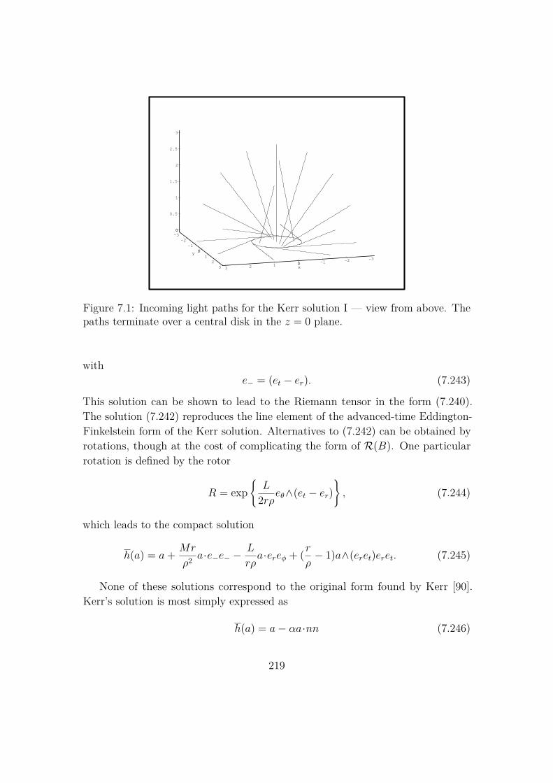
0

3

2.5

2

1.5

1

0.5

0

y 0

32

10

-1-2

-3

x0

3 2 1 0 -1 -2 -3

Figure 7.1: Incoming light paths for the Kerr solution I — view from above. Thepaths terminate over a central disk in the z = 0 plane.

withe− = (et − er). (7.243)

This solution can be shown to lead to the Riemann tensor in the form (7.240).The solution (7.242) reproduces the line element of the advanced-time Eddington-Finkelstein form of the Kerr solution. Alternatives to (7.242) can be obtained byrotations, though at the cost of complicating the form of R(B). One particularrotation is defined by the rotor

R = expL

2rρeθ∧(et − er), (7.244)

which leads to the compact solution

h(a) = a+ Mr

ρ2 a·e−e− −L

rρa·ereφ + (r

ρ− 1)a∧(eret)eret. (7.245)

None of these solutions correspond to the original form found by Kerr [90].Kerr’s solution is most simply expressed as

h(a) = a− αa·nn (7.246)

219

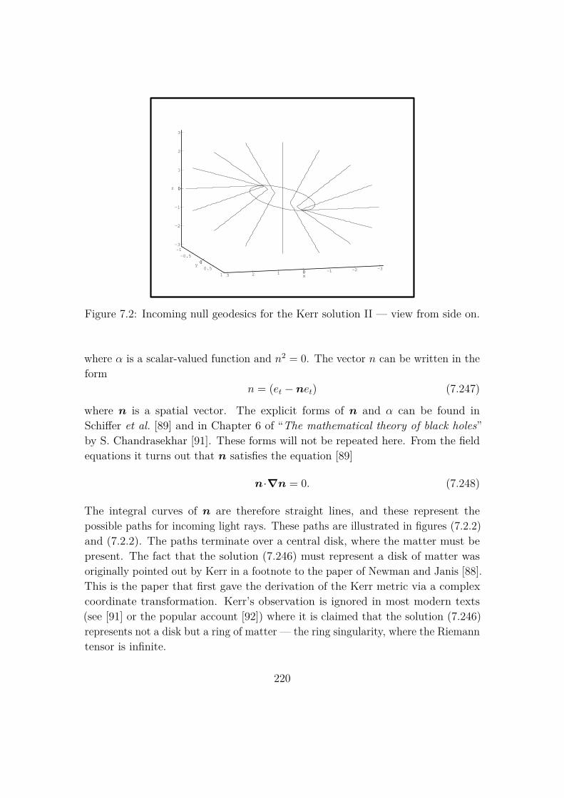
z 0

3

2

1

0

-1

-2

-3

y0

1

0.5

0

-0.5

-1

x0

3 2 1 0 -1 -2 -3

Figure 7.2: Incoming null geodesics for the Kerr solution II — view from side on.

where α is a scalar-valued function and n2 = 0. The vector n can be written in theform

n = (et − net) (7.247)

where n is a spatial vector. The explicit forms of n and α can be found inSchiffer et al. [89] and in Chapter 6 of “The mathematical theory of black holes”by S. Chandrasekhar [91]. These forms will not be repeated here. From the fieldequations it turns out that n satisfies the equation [89]

n·∇n = 0. (7.248)

The integral curves of n are therefore straight lines, and these represent thepossible paths for incoming light rays. These paths are illustrated in figures (7.2.2)and (7.2.2). The paths terminate over a central disk, where the matter must bepresent. The fact that the solution (7.246) must represent a disk of matter wasoriginally pointed out by Kerr in a footnote to the paper of Newman and Janis [88].This is the paper that first gave the derivation of the Kerr metric via a complexcoordinate transformation. Kerr’s observation is ignored in most modern texts(see [91] or the popular account [92]) where it is claimed that the solution (7.246)represents not a disk but a ring of matter — the ring singularity, where the Riemanntensor is infinite.

220

The transformations taking us from the solution (7.246) to solutions with apoint singularity involve the translation

f(x) = x′ ≡ x− L

rx·(iσ3), (7.249)

which implies that(r′)2 = r2 + L2 cos2 θ. (7.250)

Only the points for which r satisfies

r ≥ |L cos θ| (7.251)

are mapped onto points in the transformed solution, and this has the effect of cuttingout the central disk and mapping it down to a point. Curiously, the translationachieves this whilst keeping the total mass fixed (i.e. the mass parameter M isunchanged). The two types of solution (7.242) and (7.246) represent very differentmatter configurations, and it is not clear that they can really be thought of asequivalent in anything but an abstract mathematical sense.

7.3 Extended Matter DistributionsAs a final application of our flat-space gauge theory of gravity, we study howextended matter distributions are handled. We do so by concentrating on gravita-tional effects in and around stars. This is a problem that is treated very successfullyby general relativity (see [93, Chapter 23] for example) and, reassuringly, much ofthe mathematics goes through unchanged in the theory considered here. This isunsurprising, since we will assume that all effects due spin are neglible and we havealready seen that, when this is the case, the introduction of a coordinate frame willreproduce the field equations of GR. It will be clear, however, that the physics ofthe situation is quite different and the central purpose of this section is to highlightthe differences. Later in this section we discuss some aspects of rotating stars,which remains an active source of research in general relativity. Again, we work inunits where G = 1.

We start by assuming the simplest distribution of matter — that of an idealfluid. The matter stress-energy tensor then takes the form

T (a) = (ρ+ p)a·uu− pa, (7.252)

221

where ρ is the energy density, p is the pressure and u is the 4-velocity field of thefluid. We now impose a number of physical restrictions on T (a). We first assumethat the matter distribution is radially symmetric so that ρ and p are functions ofr only, where r is the (flat-space!) radial distance from the centre of the star, asdefined by (7.155). (We use translational invariance to choose the centre of the starto coincide with the spatial point that we have labelled as the origin). Furthermore,we will assume that the star is non-accelerating and can be taken as being at restwith respect to the cosmic frame (we can easily boost our final answer to take careof the case where the star is moving at a constant velocity through the cosmicmicrowave background). It follows that the velocity field u is simply et, and T nowtakes the form

T (a) = (ρ(r) + p(r))a·etet − p(r)a. (7.253)

This must equal the gravitational stress-energy tensor (the Eintein tensor), whichis generated by the h and Ω gauge fields. Radial symmetry means that h will havethe general form of (7.160). Furthermore, the form of G(a) derived from (7.160)shows that f2 and g2 must be zero, and hence that h is diagonal. This conclusioncould also have been reached by considering the motions of the underlying particlesmaking up the star. If these follow worldlines x(τ), where τ is the affine parameter,then u is defined by

u = h−1(x), (7.254)⇒ x = h(et). (7.255)

A diagonal h ensures that x is also in the et direction, so that the consituentparticles are also at rest in the 3-space relative to et. That this should be socould have been introduced as an additional physical requirement. Either way, byspecifying the details of the matter distribution we have restricted h to be of theform

h(a) = (f(r)− 1)a·etet − (g(r)− 1)a·erer + a. (7.256)

The ansätz for the gravitational fields is completed by writing

Ωt = α(r)eret Ωθ = (g(r)− 1)ereθ/rΩr = 0 Ωφ = (g(r)− 1)ereφ/r,

(7.257)

where again it is convenient to keep α(r) as a free variable, rather than solvingfor it in terms of f and g. The problem can now be solved by using the fieldequations on their own, but it is more convenient to supplement the equations with

222

the additional conditionT (D) = 0, (7.258)

which reduces to the single equation

p′(r) = αf

g(ρ+ p). (7.259)

Solving the field equations is now routine. One can either follow the method ofSection 3.1, or can simply look up the answer in any one of a number of texts. Thesolution is that

g(r) = (1− 2m(r)/r)1/2 (7.260)

wherem(r) =

∫ r

04πr′2ρ(r′) dr′. (7.261)

The pressure is found by solving the Oppenheimer-Volkov equation

p′ = −(ρ+ p)(m(r) + 4πr3p)r(r − 2m(r)) , (7.262)

subject to the condition that p(R) = 0, where R is the radius of the star. Theremaining term in h is then found by solving the differential equation

f ′(r)f(r) = −m(r) + 4πr3p

r(r − 2m(r)) (7.263)

subject to the constraint that

f(R) = (1− 2m(R)/R)−1/2. (7.264)

Finally, α(r) is given by

α(r) = (fg)−1(m(r)/r2 + 4πrp). (7.265)

The complete solution leads to a Riemann tensor of the form

R(B) = 4π [(ρ+ p)B ·etet − ρB×(eret)eret]

−m(r)2r3 (B + 3eretBeret) (7.266)

which displays a neat split into a surface term, due to the local density and pressure,

223

and a (tractionless) volume term, due to the matter contained inside the shell ofradius r.

The remarkable feature of thie solution is that (7.261) is quite clearly a flat-spaceintegral! The importance of this integral is usually downplayed in GR, but in thecontext of a flat-space theory it is entirely natural — it shows that the field outsidea sphere of radius r is determined completely by the energy density within the shell.It follows that the field outside the star is associated with a “mass” M given by

M =∫ R

04πr′2ρ(r′) dr′. (7.267)

We can understand the meaning of the definition of m(r) by considering thecovariant integral of the energy density

E0 = eti∫h−1(d3x)ρ

=∫ R

04πr′2(1− 2m(r′)/r′)−1/2ρ(r′) dr′. (7.268)

This integral is invariant under active spatial translations of the energy density.That is to say, E0 is independent of where that matter actually is. In particular,E0 could be evaluated with the matter removed to a sufficiently great distance thateach particle making up the star can be treated in isolation. It follows that E0

must be the sum of the individual mass-energies of the component particles of thestar — E0 contains no contribution from the interaction between the particles. Ifwe now expand (7.268) we find that

E0 ≈∫ R

04πr′2(ρ(r′) + ρ(r′)m(r′)/r′) dr′

= M − Potential Energy. (7.269)

The external mass M is therefore the sum of the mass-energy E0 (which ignoredinteractions) and a potential energy term. This is entirely what one expects. Gravityis due to the presence of energy, and not just (rest) mass. The effective mass seenoutside a star is therefore a combination of the mass-energies of the constituentparticles, together with the energy due to their interaction with the remainingparticles that make up the star. This is a very appealing physical picture, whichmakes complete sense within the context of a flat-space gauge theory. Furthermore,it is now clear why the definition of M is not invariant under radial translations.Interpreted actively, a radial translation changes the matter distribution within

224

the star, so the component particles are in a new configuration. It follows that thepotential energy will have changed, and so too will the total energy. An externalobserver sees this as a change in the strength of the gravitational attraction of thestar.

An important point that the above illustrates is that, given a matter distributionin the form of T (a) and (more generally) S(a), the field equations are sufficient totie down the gauge fields uniquely. Then, given any solution of the field equationG(a) = 8πT (a), a new solution can always be reached by an active transformation.But doing so alters T (a), and the new solution is appropriate to a different matterdistribution. It is meaningless to continue talking about covariance of the equationsonce the matter distribution is specified.

Whilst a non-vanishing T (a) does tie down the gauge fields, the vacuum raisesa problem. When T (a) = 0 any gauge transformation can be applied, and we seemto have no way of specifying the field outside a star, say. The resolution of thisproblem is that matter (energy) must always be present in some form, whether itbe the sun’s thermal radiation, the solar wind or, ultimately, the cosmic microwavebackground. At some level, matter is always available to tell us what the h andΩ fields are doing. This fits in with the view that spacetime itself does not playan active role in physics and it is the presence of matter, not spacetime curvature,that generates gravitational interactions.

Since our theory is based on active transformations in a flat spacetime, we cannow use local invariance to gain some insights into what the fields inside a rotatingstar might be like. To do this we rotate a static solution with a boost in the eφdirection. The rotor that achieves this is

R = expω(r, θ)φet (7.270)

whereφ ≡ eφ/(r sinθ). (7.271)

The new matter stress-energy tensor is

T (a) = (ρ+ p)a·(coshω et + sinhω φ)(coshωet + sinhω φ)− pa, (7.272)

and the Einstein tensor is similarly transformed. The stress-energy tensor (7.272)can only properly be associated with a rotating star if it carries angular momentum.The definitions of momentum and angular momentum are, in fact, quite straight-forward. The flux of momentum through the 3-space defined by a time-like vector

225

a is T (a) and the angular momentum bivector is defined by

J (a) = x∧T (a). (7.273)

Once gravitational interactions are turned on, these tensors are no longer conservedwith respect to the vector derivative,

T (∇) 6= 0, (7.274)

and instead the correct law is (7.258). This situation is analogous to that of coupledDirac-Maxwell theory (see Section 6.3). Once the fields are coupled, the individual(free-field) stress-energy tensors are no longer conserved. To recover a conservationlaw, one must either replace directional derivatives by covariant derivatives, orrealise that it is only the total stress-energy tensor that is conserved. The same istrue for gravity. Once gravitational effects are turned on, the only quantity thatone expects to be conserved is the sum of the individual matter and gravitationalstress-energy tensors. But the field equations ensure that this sum is always zero,so conservation of total energy-momentum ceases to be an issue.

If, however, a global time-like symmetry is present, one can still sensibly separatethe total (zero) energy into gravitational and matter terms. Each term is thenseparately conserved with respect to this global time. For the case of the star, thetotal 4-momentum is the sum of the individual fluxes of 4-momentum in the etdirection. We therefore define the conserved momentum P by

P =∫d3x T (et) (7.275)

and the total angular momentum J by

J =∫d3x x∧T (et). (7.276)

Concentrating on P first, we find that

P = Mrotet (7.277)

where

Mrot = 2π∫ R

0dr∫ π

0dθ r2 sin θ

[ρ(r) cosh2 ω(r, θ) + p(r) sinh2 ω(r, θ)

]. (7.278)

226

The effective mass Mrot reduces to M when the rotation vanishes, and rises withthe magnitude of ω, showing that the internal energy of the star is rising. Thetotal 4-momentum is entirely in the et direction, as it should be. Performing the Jintegral next, we obtain

J = −iσ3 2π∫ R

0dr∫ π

0dθ r3 sin2 θ (ρ(r) + p(r)) sinhω(r, θ) coshω(r, θ), (7.279)

so the angular momentum is contained in the spatial plane defined by the φetdirection. Performing an active radial boost has generated a field configurationwith suitable momentum and angular momentum properties for a rotating star.

Unfortunately, this model cannot be physical, since it does not tie down theshape of the star — an active transformation can always be used to alter the shapeto any desired configuration. The missing ingredient is that the particles makingup the star must satisfy their own geodesic equation for motion in the fields due tothe rest of the star. The simple rotation (7.270) does not achieve this.

Attention is drawn to these points for the following reason. The boost (7.270)produces a Riemann tensor at the surface of the star of

R(B) = −Mrot

2r3

(B + 3er(coshω et + sinhω φ)Ber(coshω et + sinhω φ)

),

(7.280)which is that for a rotated Schwarzschild-type solution, with a suitably modifiedmass. This form is very different to the Riemann tensor for the Kerr solution(7.240), which contains a complicated duality rotation. Whilst a physical modelwill undoubtedly require additional modifications to the Riemann tensor (7.280), itis not at all clear that these modifications will force the Riemann tensor to be ofKerr type. Indeed, the differences between the respective Riemann tensors wouldappear to make this quite unlikely. The suggestion that a rotating star does notcouple onto a Kerr-type solution is strengthened by the fact that, in the 30 or soyears since the discovery of the Kerr solution [90], no-one has yet found a solutionfor a rotating star that matches onto the Kerr geometry at its boundary.

7.4 ConclusionsThe gauge theory of gravity developed from the Dirac equation has a number ofinteresting and surprising features. The requirement that the gravitational actionshould be consistent with the Dirac equation leads to a unique choice for the action

227

integral (up to the possible inclusion of a cosmological constant). The result isa set of equations which are first-order in the derivatives of the fields. This is incontrast to general relativity, which is a theory based on a set of second-orderpartial differential equations for the metric tensor. Despite the formal similaritiesbetween the theories, the study of point-source solutions reveals clear differences.In particular, the first-order theory does not admit solutions which are invariantunder time-reversal.

The fact that the gauge group consists of active Poincaré transformationsof spacetime fields means that gauge transformations relate physically distinctsituations. It follows that observations can determine the nature of the h and Ωfields. This contrasts with Yang-Mills theories based on internal gauge groups,where one expects that all observables should be gauge-invariant. In this context, animportant open problem is to ascertain how the details of radial collapse determinethe precise nature of the h and Ω fields around a black hole.

A strong point in favour of the approach developed here is the great formal claritythat geometric algebra brings to the study of the equations. This is illustrated mostclearly in the compact formulae for the Riemann tensor for the Schwarzschild andKerr solutions and for radially-symmetric stars. No rival method (tensor calculus,differential forms, Newman-Penrose formalism) can offer such concise expressions.

For 80 years, general relativity has provided a successful framework for the studyof gravitational interactions. Any departure from it must be well-motivated bysound physical and mathematical reasons. The mathematical arguments in favourof the present approach include the simple manner in which transformations arehandled, the algebraic compactness of many formulae and the fact that torsion isperhaps better viewed as a spacetime field than as a geometric effect. Elsewhere, anumber of authors have questioned whether the view that gravitational interactionsare the result of spacetime geometry is correct (see [94], for example). The physicalmotivation behind the present theory is provided by the identification of the h andΩ fields as the dynamical variables. The physical structure of general relativityis very much that of a classical field theory. Every particle contributes to thecurvature of spacetime, and every particle moves on the resultant curved manifold.The picture is analogous to that of electromagnetism, in which all charged particlescontribute to an electromagnetic field (a kind of global ledger). Yet an apparentlycrucial step in the development of Q.E.D. was Feynman’s realisation (together withWheeler [95, 96]) that the electromagnetic field can be eliminated from classicalelectrodynamics altogether. A similar process may be required before a quantummultiparticle theory of gravity can be constructed. In the words of Einstein [97]

228

. . . the energy tensor can be regarded only as a provisional means ofrepresenting matter. In reality, matter consists of electrically chargedparticles . . .

The status of the h and Ω fields can be regarded as equally provisional. They maysimply represent the aggregate behaviour of a large number of particles, and assuch would not be of fundamental significance. In this case it would be wrong toattach too strong a physical interpretation to these fields (i.e. that they are theresult of spacetime curvature and torsion).

An idea of how the h field could arise from direct interparticle forces is providedby the two-particle Dirac action constructed in Section 6.3. There the actionintegral involved the differential operator ∇1/m1 + ∇2/m2, so that the vectorderivatives in each particle space are weighted by the mass of the particle. Thisbegins to suggest a mechanism by which, at the one-particle level, the operatorh(∇) encodes an inertial drag due to the other particle in the universe. Thisis plausible, as the h field was originally motivated by considering the effect oftranslating a field. The theory presented here does appear to contain the correctingredients for a generalisation to a multiparticle quantum theory, though onlytime will tell if this possibility can be realised.

229

Bibliography

[1] A.N. Lasenby, C.J.L. Doran, and S.F. Gull. Grassmann calculus, pseudoclassi-cal mechanics and geometric algebra. J. Math. Phys., 34(8):3683, 1993.

[2] C.J.L. Doran, D. Hestenes, F. Sommen, and N. van Acker. Lie groups as spingroups. J. Math. Phys., 34(8):3642, 1993.

[3] C.J.L. Doran, A.N. Lasenby, and S.F. Gull. Grassmann mechanics, mul-tivector derivatives and geometric algebra. In Z. Oziewicz, B. Jancewicz,and A. Borowiec, editors, Spinors, Twistors, Clifford Algebras and QuantumDeformations, page 215. Kluwer Academic, Dordrecht, 1993.

[4] A.N. Lasenby, C.J.L. Doran, and S.F. Gull. 2-spinors, twistors and supersym-metry in the spacetime algebra. In Z. Oziewicz, B. Jancewicz, and A. Borowiec,editors, Spinors, Twistors, Clifford Algebras and Quantum Deformations, page233. Kluwer Academic, Dordrecht, 1993.

[5] S.F. Gull, A.N. Lasenby, and C.J.L. Doran. Imaginary numbers are not real —the geometric algebra of spacetime. Found. Phys., 23(9):1175, 1993.

[6] C.J.L. Doran, A.N. Lasenby, and S.F. Gull. States and operators in thespacetime algebra. Found. Phys., 23(9):1239, 1993.

[7] A.N. Lasenby, C.J.L. Doran, and S.F. Gull. A multivector derivative approachto Lagrangian field theory. Found. Phys., 23(10):1295, 1993.

[8] S.F. Gull, A.N. Lasenby, and C.J.L. Doran. Electron paths, tunnelling anddiffraction in the spacetime algebra. Found. Phys., 23(10):1329, 1993.

[9] C.J.L. Doran, A.N. Lasenby, and S.F. Gull. Gravity as a gauge theory in thespacetime algebra. In F. Brackx, R. Delanghe, and H. Serras, editors, CliffordAlgebras and their Applications in Mathematical Physics (1993), page 375.Kluwer Academic, Dordrecht, 1993.

230

[10] A.N. Lasenby, C.J.L. Doran, and S.F. Gull. Cosmological consequences of aflat-space theory of gravity. In F. Brackx, R. Delanghe, and H. Serras, editors,Clifford Algebras and their Applications in Mathematical Physics (1993), page387. Kluwer Academic, Dordrecht, 1993.

[11] M.F. Atiyah, R. Bott, and A. Shapiro. Clifford modules. Topology, 3(Supp.1):3, 1964.

[12] I.R. Porteous. Topological Geometry. Van Nostrand Reinhold Company, 1969.

[13] I.W. Benn and R.W. Tucker. An Introduction to Spinors and Geometry. AdamHilger, Bristol, 1988.

[14] C. Chevalley. The Algebraic Theory of Spinors. Columbia University Press,1954.

[15] H.B. Lawson and M.-L. Michelsohn. Spin Geometry. Princeton UniversityPress, Princeton NJ, 1989.

[16] F. Reese. Harvey. Spinors and Calibrations. Academic Press, San Diego, 1990.

[17] D. Hestenes. Space–Time Algebra. Gordon and Breach, New York, 1966.

[18] D. Hestenes. Multivector calculus. J. Math. Anal. Appl., 24:313, 1968.

[19] D. Hestenes. Vectors, spinors, and complex numbers in classical and quantumphysics. Am. J. Phys., 39:1013, 1971.

[20] D. Hestenes. Proper dynamics of a rigid point particle. J. Math. Phys.,15(10):1778, 1974.

[21] D. Hestenes. Observables, operators, and complex numbers in the Dirac theory.J. Math. Phys., 16(3):556, 1975.

[22] D. Hestenes and R. Gurtler. Consistency in the formulation of the Dirac, Pauliand Schrödinger theories. J. Math. Phys., 16(3):573, 1975.

[23] D. Hestenes. Spin and uncertainty in the interpretation of quantum mechanics.Am. J. Phys., 47(5):399, 1979.

[24] D. Hestenes and G. Sobczyk. Clifford Algebra to Geometric Calculus. Reidel,Dordrecht, 1984.

231

[25] D. Hestenes. New Foundations for Classical Mechanics (Second Edition).Kluwer Academic Publishers, Dordrecht, 1999.

[26] D. Hestenes. A unified language for mathematics and physics. In J.S.R.Chisholm and A.K. Common, editors, Clifford Algebras and their Applicationsin Mathematical Physics (1985), page 1. Reidel, Dordrecht, 1986.

[27] D. Hestenes. Clifford algebra and the interpretation of quantum mechanics.In J.S.R. Chisholm and A.K. Common, editors, Clifford Algebras and theirApplications in Mathematical Physics (1985), page 321. Reidel, Dordrecht,1986.

[28] D. Hestenes. Curvature calculations with spacetime algebra. Int. J. Theor.Phys., 25(6):581, 1986.

[29] D. Hestenes. On decoupling probability from kinematics in quantum mechanics.In P. Fougère, editor, Maximum Entropy and Bayesian Methods, page 161.Kluwer Academic, Dordrecht, 1990.

[30] D. Hestenes. The design of linear algebra and geometry. Acta Appl. Math.,23:65, 1991.

[31] D. Hestenes and R. Ziegler. Projective geometry with Clifford algebra. Acta.Appli. Math., 23:25, 1991.

[32] D. Hestenes. Hamiltonian mechanics with geometric calculus. In Z. Oziewicz,B. Jancewicz, and A. Borowiec, editors, Spinors, Twistors, Clifford Algebrasand Quantum Deformations, page 203. Kluwer Academic, Dordrecht, 1993.

[33] D. Hestenes. Real Dirac theory. In Preparation, 1994.

[34] D. Hestenes. Differential forms in geometric calculus. In F. Brackx, R. Delanghe,and H. Serras, editors, Clifford Algebras and their Applications in MathematicalPhysics (1993), page 269. Kluwer Academic, Dordrecht, 1993.

[35] F.A. Berezin. The Method of Second Quantization. Academic Press Ltd.,London, 1966.

[36] R. Penrose and W. Rindler. Spinors and space-time, Volume I: two-spinorcalculus and relativistic fields. Cambridge University Press, 1984.

232

[37] R. Penrose and W. Rindler. Spinors and space-time, Volume II: spinor andtwistor methods in space-time geometry. Cambridge University Press, 1986.

[38] A.O. Barut and N. Zanghi. Classical models of the Dirac electron. Phys. Rev.Lett., 52(23):2009, 1984.

[39] F.A. Berezin and M.S. Marinov. Particle spin dynamics as the Grassmannvariant of classical mechanics. Ann. Phys., 104:336, 1977.

[40] M. Kline. Mathematical Thought from Ancient to Modern Times. OxfordUniversity Press, 1972.

[41] H. Grassmann. Der ort der Hamilton’schen quaternionen in der Ausdehnung-slehre. Math. Ann., 12:375, 1877.

[42] W.K. Clifford. Applications of Grassmann’s extensive algebra. Am. J. Math.,1:350, 1878.

[43] M.F. Atiyah and I.M. Singer. The index of elliptic operators on compactmanifolds. Bull. A.M.S., 69:422, 1963.

[44] T.G. Vold. An introduction to geometric algebra with an application to rigidbody mechanics. Am. J. Phys., 61(6):491, 1993.

[45] T.G. Vold. An introduction to geometric calculus and its application toelectrodynamics. Am. J. Phys., 61(6):505, 1993.

[46] R. Ablamovicz, P. Lounesto, and J. Maks. Second workshop on Clifford algebrasand their applications in mathematical physics. Found. Phys., 21(6):735, 1991.

[47] E.T. Jaynes. Scattering of light by free electrons. In A. Weingartshofer andD. Hestenes, editors, The Electron, page 1. Kluwer Academic, Dordrecht, 1991.

[48] N. Salingaros. On the classification of Clifford algebras and their relation tospinors in n-dimensions. J. Math. Phys., 23(1):1, 1982.

[49] I. Stewart. Hermann grassmann was right (News and Views). Nature, 321:17,1986.

[50] M. Barnabei, A. Brini, and G.-C. Rota. On the exterior calculus of invarianttheory. J. Algebra, 96:120, 1985.

[51] F.A. Berezin. Introduction to Superanalysis. Reidel, Dordrecht, 1987.

233

[52] B. de Witt. Supermanifolds. Cambridge University Press, 1984.

[53] R. Coquereaux, A. Jadczyk, and D. Kastler. Differential and integral geometryof Grassmann algebras. Reviews in Math. Phys., 3(1):63, 1991.

[54] A. Connes and J. Lott. Particle models and non-commutative geometry. Nucl.Phys. B (Proc. Suppl.), 18B:29, 1990.

[55] G.C. Sherry. A generalised phase space for classical fermions arising out ofSchonberg’s geometric algebras. Found. Phys. Lett., 2(6):591, 1989.

[56] G.C. Sherry. Algebraic model of a classical non-relativistic electron. Found.Phys. Lett., 3(3):267, 1990.

[57] J.F. Cornwell. Group Theory in Phsics II. Academic Press Ltd., London,1984.

[58] A.O. Barut and A.J. Bracken. The remarkable algebra so∗(2n), its represen-tations, its Clifford algebra and potential applications. J. Phys. A, 23:641,1990.

[59] J.D. Bjorken and S.D. Drell. Relativistic Quantum Mechanics, vol 1. McGraw-Hill, New York, 1964.

[60] C. Itzykson and J-B. Zuber. Quantum Field Theory. McGraw–Hill, New York,1980.

[61] S.F. Gull. Charged particles at potential steps. In A. Weingartshofer andD. Hestenes, editors, The Electron, page 37. Kluwer Academic, Dordrecht,1991.

[62] E.M. Corson. Introduction to Tensors, Spinors, and Relativistic Wave-Equations. Blackie & Son, Ltd., Glasgow, 1953.

[63] A.P. Galeao and P. Leal Ferreira. General method for reducing the two-bodyDirac equation. J. Math. Phys., 33(7):2618, 1992.

[64] E.E. Salpeter and H.A. Bethe. A relativistic equation for bound-state problems.Phys. Rev., 84(6):1232, 1951.

[65] G. Breit. The effect of retardation on the interaction of two electrons. Phys.Rev., 34(4):553, 1929.

234

[66] N. Kemmer. Zur theorie der neutron-proton wechselwirkung. Helv. Phys.Acta., 10:48, 1937.

[67] E. Fermi and C.N. Yang. Are mesons elementary particles? Phys. Rev.,76(12):1739, 1949.

[68] Y. Koide. Exactly solvable model of relativistic wave equations and mesonspectra. Il Nuovo Cim., 70A(4):411, 1982.

[69] W. Królikowski. Duffin–Kemmer–Petiau particle with internal structure. ActaPhys. Pol. B, 18(2):111, 1987.

[70] W. Królikowski. Clifford algebras and the algebraic structure of fundamentalfermions. In Z. Oziewicz, B. Jancewicz, and A. Borowiec, editors, Spinors,Twistors, Clifford Algebras and Quantum Deformations, page 183. KluwerAcademic, Dordrecht, 1993.

[71] H. Goldstein. Classical Mechanics. Addison–Wesley, Reading MA, 1950.

[72] J.W. van Holten. On the electrodynamics of spinning particles. Nucl. Phys.,B356(3):3, 1991.

[73] P.G.O. Freund. Supersymmetry. Cambridge University Press, 1986.

[74] R. Casalbuoni. The classical mechanics for Bose-Fermi systems. Il NuovoCimento., 33A(3):389, 1976.

[75] L. Brink, S. Deser, B. Zumino, P. di Vecchia, and P. Howe. Local supersym-metry for spinning particles. Phys. lett. B, 64(4):435, 1976.

[76] J.F. Cornwell. Group Theory in Physics III. Academic Press Ltd., London,1989.

[77] S. Coleman. Aspects of Symmetry. Cambridge University Press, 1985.

[78] H. Tetrode. Der impuls-energiesatz in der Diracschen quantentheorie deselektrons. Z. Physik, 49:858, 1928.

[79] R. Utiyama. Invariant theoretical interpretation of interaction. Phys. Rev.,101(5):1597, 1956.

[80] T.W.B. Kibble. Lorentz invariance and the gravitational field. J. Math. Phys.,2(3):212, 1961.

235

[81] F.W. Hehl, P. von der Heyde, G.D. Kerlick, and J.M. Nester. General relativitywith spin and torsion: Foundations and prospects. Rev. Mod. Phys., 48:393,1976.

[82] D. Ivanenko and G. Sardanashvily. The gauge treatment of gravity. Phys.Rep., 94(1):1, 1983.

[83] S.W. Hawking and G.F.R. Ellis. The Large Scale Structure of Space-Time.Cambridge University Press, 1973.

[84] R.T. Rauch. Equivalence of an R +R2 theory of gravity to Einstein–Cartan–Sciama–Kibble theory in the presence of matter. Phys. Rev. D, 26(4):931,1982.

[85] R.D. Hecht, J. Lemke, and R.P. Wallner. Can Poincaré gauge theory be saved?Phys. Rev. D, 44(8):2442, 1991.

[86] A.V. Khodunov and V.V. Zhytnikov. Gravitational equations in space-timewith torsion. J. Math. Phys., 33(10):3509, 1992.

[87] R. d’Inverno. Introducing Einstein’s Relativity. Oxford University Press, 1992.

[88] E.T. Newman and A.I. Janis. Note on the Kerr spinning-particle metric.J. Math. Phys., 6(4):915, 1965.

[89] M.M. Schiffer, R.J. Adler, J. Mark, and C. Sheffield. Kerr geometry ascomplexified Schwarzschild geometry. J. Math. Phys., 14(1):52, 1973.

[90] R.P. Kerr. Gravitational field of a spinning mass as an example of algebraicallyspecial metrics. Phys. Rev. Lett., 11(5):237, 1963.

[91] S. Chandrasekhar. The Mathematical Theory of Black Holes. Oxford UniversityPress, Oxford, 1983.

[92] W.J. Kaufmann. The Cosmic Frontiers of General Relativity. Penguin Books,1979.

[93] C.W. Misner, K.S. Thorne, and J.A. Wheeler. Gravitation. W.H. Freemanand Company, San Francisco, 1973.

[94] S. Weinberg. Gravitation and Cosmology. Wiley, New York, 1972.

236

[95] J.A. Wheeler and R.P. Feynman. Interaction with the absorber as the mecha-nism of radiation. Rev. Mod. Phys., 17:157, 1945.

[96] J.A. Wheeler and R.P. Feynman. Classical electrodynamics in terms of directinterparticle action. Rev. Mod. Phys., 21(3):425, 1949.

[97] A. Einstein. The Meaning of Relativity. Princeton University Press, PrincetonNJ, 1945.

237